nonnegative matrix factorization - algorithms and …nonnegative matrix factorization (nmf). for...
TRANSCRIPT
UNIVERSITÉ CATHOLIQUE DE LOUVAIN
ÉCOLE POLYTECHNIQUE DE LOUVAIN
DÉPARTEMENT D’INGÉNIERIE MATHÉMATIQUE
NONNEGATIVE MATRIX FACTORIZATIONALGORITHMS AND APPLICATIONS
NGOC-DIEP HO
Thesis submitted in partial fulfillmentof the requirements for the degree ofDocteur en Sciences de l’Ingénieur
Dissertation committee:Prof. Vincent Wertz (President)Prof. Paul Van Dooren (Promoter)Prof. Vincent Blondel (Promoter)Prof. François GlineurProf. Yurii NesterovProf. Bob PlemmonsProf. Johan Suykens
June 2008


ACKNOWLEDGMENTS
First, I would like to thank Prof. Paul Van Dooren and Prof. VincentBlondel for the five long years as my advisors. Your support and advicehave guided me through the most difficult moments of my research.Not only me, everyone will be really proud to have advisors like you.Paul and Vincent, thanks for your precious presence.
I am thankful to Prof. François Glineur, Prof. Yurii Nesterov, Prof.Bob Plemmons, Prof. Johan Suykens and Prof. Vincent Wertz for beingon my dissertation committee.
Many thanks to the Centre for Systems Engineering and AppliedMechanics for providing me an excellent research environment, espe-cially to Isabelle, Lydia and Michou and Etienne for their administrativeand technical assistance and to all the members of the research group onLarge Graphs and Networks for all activities both at work and off work.
I am also grateful to the small Vietnamese community and theirfriends in Louvain-la-Neuve for their help, to Alain and Frédérique whoare simply very special.
Above all, I send my thanks to all my family in Vietnam for their dailysupport and I want to dedicate this thesis to my wife Hang, my daughter Maiand my son Nam who are always by my side.

iv ACKNOWLEDGMENTS
This research has been supported by the Belgian Programme onInter-university Poles of Attraction, initiated by the Belgian State, PrimeMinister’s Office for Science, Technology and Culture. It has been alsosupported by the ARC (Concerted Research Action) Large Graphs andNetworks, of the French Community of Belgium. I was also a FRIAfellow (Fonds pour la formation à la Recherche dans l’Industrie et dansl’Agriculture).
TABLE OF CONTENTS
Acknowledgments iii
Table of contents vi
Notation glossary vii
Introduction 1
1 Preliminaries 131.1 Matrix theory and linear algebra . . . . . . . . . . . . . . 131.2 Optimization . . . . . . . . . . . . . . . . . . . . . . . . . . 211.3 Low-rank matrix approximation . . . . . . . . . . . . . . 26
2 Nonnegative matrix factorization 332.1 Problem statement . . . . . . . . . . . . . . . . . . . . . . 332.2 Solution . . . . . . . . . . . . . . . . . . . . . . . . . . . . 392.3 Exact factorization and nonnegative rank . . . . . . . . . 432.4 Extensions of nonnegative matrix factorization . . . . . . 46
3 Existing algorithms 493.1 Lee and Seung algorithm . . . . . . . . . . . . . . . . . . . 513.2 Alternating least squares methods . . . . . . . . . . . . . 553.3 Gradient descent . . . . . . . . . . . . . . . . . . . . . . . 573.4 Scaling and stopping criterion . . . . . . . . . . . . . . . . 613.5 Initializations . . . . . . . . . . . . . . . . . . . . . . . . . 63
4 Rank-one residue iteration 654.1 Motivation . . . . . . . . . . . . . . . . . . . . . . . . . . . 65
vi TABLE OF CONTENTS
4.2 Column partition of variables . . . . . . . . . . . . . . . . 674.3 Convergence . . . . . . . . . . . . . . . . . . . . . . . . . . 704.4 Variants of the RRI method . . . . . . . . . . . . . . . . . 744.5 Regularizations . . . . . . . . . . . . . . . . . . . . . . . . 764.6 Algorithms for NMF extensions . . . . . . . . . . . . . . . 784.7 Numerical experiments . . . . . . . . . . . . . . . . . . . . 81
5 Nonnegative matrix factorization with fixed row and columnsums 995.1 Problem statement . . . . . . . . . . . . . . . . . . . . . . 1005.2 Generalized KL divergence in NMF . . . . . . . . . . . . 1025.3 Application: stochastic matrix approximation . . . . . . . 109
6 Weights in nonnegative matrix factorization 1116.1 Gradient information . . . . . . . . . . . . . . . . . . . . . 1126.2 Methods . . . . . . . . . . . . . . . . . . . . . . . . . . . . 1136.3 Toward the weighted KL divergence . . . . . . . . . . . . 1206.4 Adding weights to existing NMF variants . . . . . . . . . 1246.5 Application: feature extraction of face images . . . . . . . 125
7 Symmetry in nonnegative matrix factorization 1317.1 Symmetric approximations . . . . . . . . . . . . . . . . . 1327.2 Methods . . . . . . . . . . . . . . . . . . . . . . . . . . . . 1377.3 Applications: graph clustering . . . . . . . . . . . . . . . 1507.4 Application: correlation matrix approximation . . . . . . 154
Conclusion 161
Bibliography 165
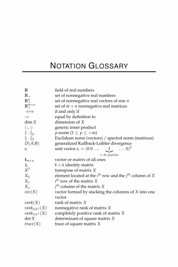
NOTATION GLOSSARY
R field of real numbersR+ set of nonnegative real numbersRn
+ set of nonnegative real vectors of size nRm×n
+ set of m× n nonnegative real matrices⇐⇒ if and only if
:= equal by definition todim X dimension of X〈·, ·〉 generic inner product‖ · ‖p p-norm (1 ≤ p ≤ +∞)‖ · ‖2 Euclidean norm (vectors) / spectral norm (matrices)D(A|B) generalized Kullback-Leibler divergenceei unit vector ei = (0 0 . . . 1︸︷︷︸
i−th position
. . . 0)T
1m×n vector or matrix of all onesIk k× k identity matrixXT transpose of matrix XXij element located at the ith row and the jth column of XXi: ith row of the matrix XX:j jth column of the matrix Xvec(X) vector formed by stacking the columns of X into one
vectorrank(X) rank of matrix XrankUVT (X) nonnegative rank of matrix XrankVVT (X) completely positive rank of matrix Xdet X determinant of square matrix Xtrace(X) trace of square matrix X
viii NOTATION GLOSSARY
λk(X) k-th eigenvalue of matrix Xσ(X) set of eigenvalues of the matrix Xρ(X) maxi |λi(X)|σmax(X) maximal singular value of matrix Xσmin(X) minimal singular value of matrix XA⊗ B Kronecker product between matrices A and BA B Hadamard product between matrices A and B[A][B]
Hadamard division between matrices A and B
[A]+ projection of A onto the nonnegative orthantD(v) diagonal matrix with v on the main diagonal
Abbreviations and acronyms
NMF Nonnegative Matrix FactorizationSNMF Symmetric Nonnegative Matrix FactorizationSSNMF Semi-Symmetric Nonnegative Matrix FactorizationWNMF Weighted Nonnegative Matrix FactorizationSVD Singular Value Decomposition
INTRODUCTION
In every single second in this modern era, tons of data are being gener-ated. Think of the number of online people writing their blogs, designingtheir homepages and sharing their experiences through many other dig-ital supports: videos, photos, etc. Think also of the data generated whendecoding genes of living creatures and the data acquired from the outerspace or even from our own planet, etc.
Data only become useful when having been processed. In front ofthis fast-growing amount of data, there are several approaches for dataprocessing: applying classical methods, designing more powerful com-puting structures such as distributed computing, multicore processors,supercomputers, etc. But the growing amount and complexity of accu-mulated data seems to outweigh the growth of computing power whichis, at the present time, roughly doubling every year (cfr. Moore’s Law[90]). One very popular approach is called model reduction which triesto reduce the complexity while keeping the essentials of the problem (ordata).
Besides, different types of data require different models to capturethe insight of the data. Using the right model saves a lot of time. Ofcourse, a model believed to be right will stand until a better model isfound. An ideal model may not exist. For instance, using dominantsubspaces with the Singular Value Decomposition (SVD) [50] has beenproposed as the best model to reduce the complexity of data and compli-cated systems. It offers the least error (with respect to some measures)with the same reduced complexity, compared to other models. Butit is not the only one since the conic representation or conic coding[82] is also extensively used. Its properties favour the additive model ofsome types of data while SVD-related techniques do not. In this thesis,
INTRODUCTION
we focus on finding the best reduced conic representation of nonnega-tive data through Nonnegative Matrix Factorization (NMF). We will gothrough several issues that are considered as the building blocks for thenonnegative matrix factorization (NMF).
For nonnegative data, we will see that this additive model offers acloser physical representation to the reality than other techniques such asthe SVDs. But this is not for free. On the one hand, SVD decompositionis known to have polynomial-time complexity. In fact, it can be done ina polynomial number, i.e. nm min(m, n), of basic operations for a fulldecomposition, where n and m are the dimensions of the matrix data [50].When only a partial SVD decomposition is needed, iterative methodscan be applied with the computational load of mnr basic operations periteration, where r, 1 ≥ r ≥ min(m, n), is the reduced dimension of thedecomposition. Their convergence speed, represented by the number ofiterations needed, has been being improved drastically, which allowsus to process massive data sets. On the other hand, NMF factorizationhas been recently proved to have a nondeterministic polynomial - NPcomputational complexity [121] for which the existence of a polynomial-time optimal algorithm is unknown. However, iterative methods withlow computational load iterations are still possible. There are iterativemethods whose computational load per iteration is roughly equivalentto the one of SVD, i.e. mnr, such as [81], [86], etc. as well as the onedescribed in this thesis. But only acceptable solutions are expected ratherthan the optimal one. And restarts maybe needed. The main aspectsthat differentiate these methods are then: to which solution they tend toconverge? how fast they converge? and how to drive them to converge tosolutions that possess some desired properties?
Part-based analysis
An ordinary object is usually a collection of simple parts connected bysome relations between them. Building objects from basic parts is one ofthe simplest principle applicable to many human activities. Moreover,human vision is designed to be able to detect the presence or the absenceof features (parts) of a physical object. Thanks to these parts, a humancan recognize and distinguish most of the objects [15].
INTRODUCTION
Without taking into account the possible relations between partsand assuming that we can establish a full list of all possible parts of allpossible objects, then there is one unified formula for composing theobjects:
Objecti = Part1(bi1) with Part2(bi2) with . . . ,
where
bij =
present if part i is present in object jabsent if part i is absent from object j.
Then we can represent object i by a list (bi1, bi2, . . .) that can be simplifiedby replacing the status present and absent by 1 and 0. This model can beimproved by taking into account the quantity of parts inside an object.The final recipe for making an object is then something like
Objecti = bi1 × Part1 + bi2 × Part2 + . . .
where bij ≥ 0.In reality, only some objects are available through observations. The
task is then to detect parts from observed objects and to use the detectedparts to reconstitute these objects. This simple idea appears in manyapplications and will be illustrated in the following examples.
Image learning
Digital image processing has been a hot topic in recent years. Thisincludes face recognition [54], optical character recognition [70], content-based image retrieval [109], etc. Each monochrome digital image is arectangular array of pixels. And each pixel is represented by its light in-tensity. Since the light intensity is measured by a nonnegative value, wecan represent each image as a nonnegative matrix, where each elementis a pixel. Color images can be coded in the same way but with severalnonnegative matrices.
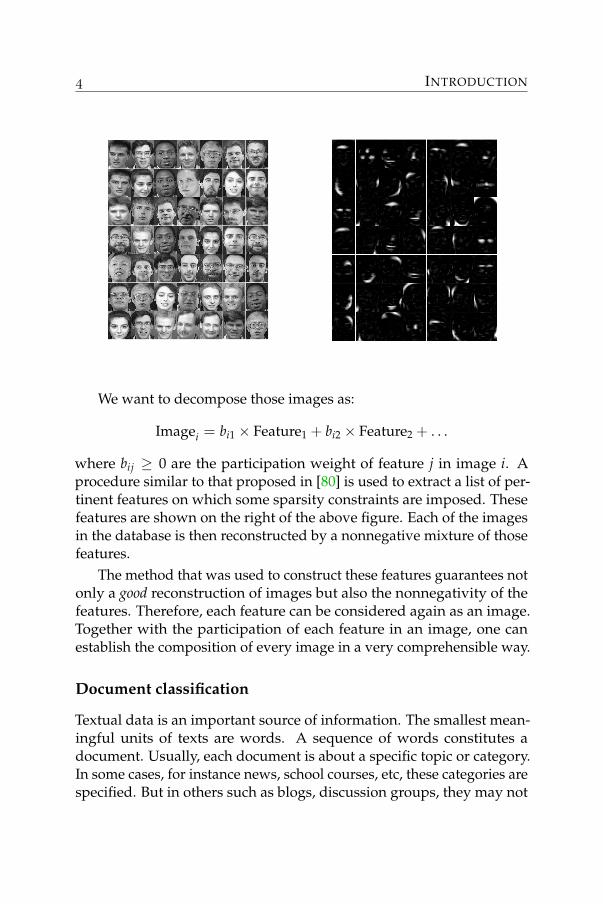
An example is the Cambridge ORL face database. It contains 400monochrome images of a front view of the face of 40 persons (10 imagesper person). The size of each image is 112× 92 with 256 gray levelsper pixel. Some randomly selected images are shown on the left of thefollowing figure.
INTRODUCTION
We want to decompose those images as:
Imagei = bi1 × Feature1 + bi2 × Feature2 + . . .
where bij ≥ 0 are the participation weight of feature j in image i. Aprocedure similar to that proposed in [80] is used to extract a list of per-tinent features on which some sparsity constraints are imposed. Thesefeatures are shown on the right of the above figure. Each of the imagesin the database is then reconstructed by a nonnegative mixture of thosefeatures.
The method that was used to construct these features guarantees notonly a good reconstruction of images but also the nonnegativity of thefeatures. Therefore, each feature can be considered again as an image.Together with the participation of each feature in an image, one canestablish the composition of every image in a very comprehensible way.
Document classification
Textual data is an important source of information. The smallest mean-ingful units of texts are words. A sequence of words constitutes adocument. Usually, each document is about a specific topic or category.In some cases, for instance news, school courses, etc, these categories arespecified. But in others such as blogs, discussion groups, they may not
INTRODUCTION
Topic 1 Topic 2 Topic 3 Topic 4court president flowers disease
government served leaves behaviorcouncil governor plant glandsculture secretary perennial contact
supreme senate flower symptomsconstitutional congress plants skin
rights presidential growing painjustice elected annual infection
be listed. Moreover, a classification is hardly unique, several differentclassifications can be defined. For instance, news articles can be classi-fied not only with topics such as: economics, cultures, sports, sciences,etc. but also according to the geographical regions (Asia, Europe, Africa,etc).
Without a grammar, a text can be seen as a set of words combinedwith their number of occurrences. Given a collection of texts, one wantsto automatically discover the hidden classifications. The task is then totry to explain a text as:
Texti = bi1 × Topic1 + bi2 × Topic2 + . . .
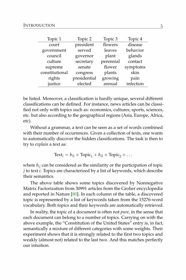
where bij can be considered as the similarity or the participation of topicj to text i. Topics are characterized by a list of keywords, which describetheir semantics.
The above table shows some topics discovered by NonnegativeMatrix Factorization from 30991 articles from the Grolier encyclopediaand reported in Nature [80]. In each column of the table, a discoveredtopic is represented by a list of keywords taken from the 15276-wordvocabulary. Both topics and their keywords are automatically retrieved.
In reality, the topic of a document is often not pure, in the sense thateach document can belong to a number of topics. Carrying on with theabove example, the “Constitution of the United States” entry is, in fact,semantically a mixture of different categories with some weights. Theirexperiment shows that it is strongly related to the first two topics andweakly (almost not) related to the last two. And this matches perfectlyour intuition.
INTRODUCTION
Having discovered a list of topics and their participation in eachdocument, one can not only decide to which topics a document belongs,but also deal with the polysemy of words, detect new trends, revealhidden categories, etc.
Why nonnegativity?
As we have seen, for the part-based analysis, the presence or absenceof parts creates recipes for making an object. This existential status ofparts is represented by nonnegative numbers, where 0 represents anabsence and a positive number represents a presence with some degree.Furthermore, the objects are also represented by a set of nonnegativenumbers, e.g., numbers of occurrences or light intensities. Because ofthat, nonnegativity is a crucial feature that one needs to maintain duringthe analysis of objects.
The part-based analysis is also referred to as the additive modelbecause of the absence of subtractions in the model. This follows fromthe construction of an object:
Objecti = bi1 × Part1 + bi2 × Part2 + . . .
Allowing subtractions, i.e., bij < 0 for some i, j implies that any part canbe interpreted as either a positive or a negative quantity. When eachpart belongs to a vector space, this is true since the orientation doesnot change the spanning space. But for other types of data such as: theconcentrations of substances, absolute temperatures, light intensities,probabilities, sound spectra, etc. negative quantities do not arise. De-composing nonnegative objects with general methods like the SingularValue Decomposition significantly alters the physical interpretation of thedata. Other analysis tools like the Principal Component Analysis requiresome features which nonnegative objects by their nature never or hardlypossess, such as zero sum, orthogonality etc.
While much evidence from existing applications shows the appeal ofthe part-based method, the lack of algorithmic understandings prohibitsextensions to larger scale problems and to other types of data. This gaveus enough motivations to focus on a better tool for nonnegative datathrough a thorough study of nonnegative matrix factorization. This tech-nique allows us to approximate nonnegative objects, stored in columns
INTRODUCTION
of a nonnegative matrix A, by the product of two other nonnegativematrices U and V:
A ≈ UVT.
This factorization captures all the key ideas from the above examplesof the part-based analysis. Columns of U define the extracted parts (orimage features or document topics, etc.). The matrix V describes theparticipations of those parts in the original objects (or images, document,etc.).
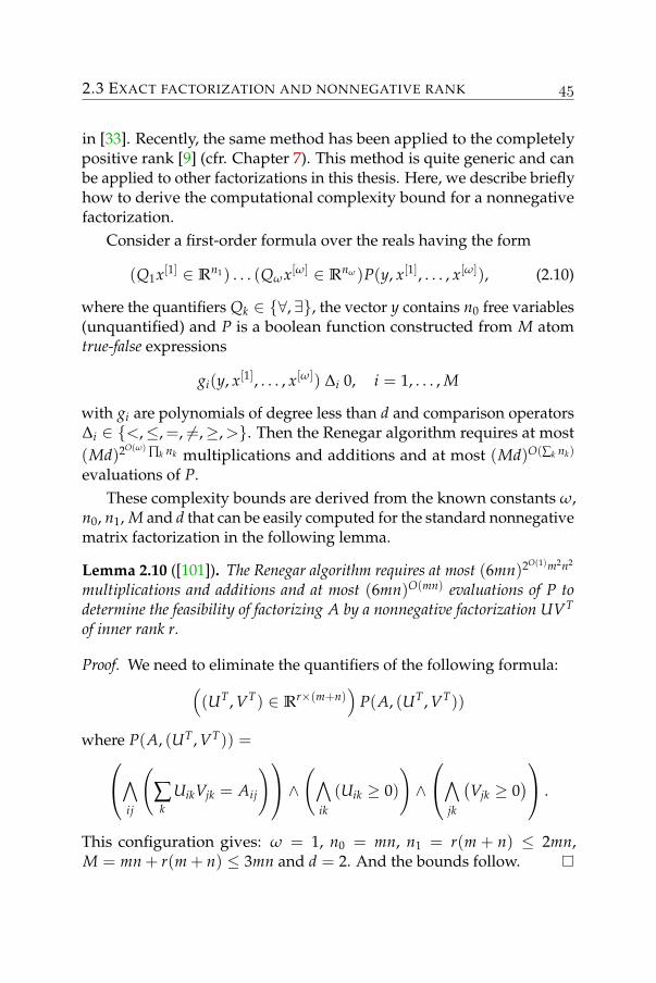
The idea of approximating a nonnegative matrix A by the productUVT of two nonnegative matrices U and V is not new. In fact, it isa generalized method of the well-known K-Means method [88] from1967, applied to nonnegative data. Suppose we have n nonnegative datavectors a1,. . . , an and r initial centroids u1, . . . , ur representing r clustersC1, . . . , Cr, what the K-Means method does is to repeat the followingtwo steps until convergence:
1. For each ai, assign it to Cj if uj is the nearest centroid to ai,with respect to Euclidean distance.
2. For each uj, replace it with the arithmetic mean of all ai inCj.
We can construct a matrix U by putting all the vectors uj in thecolumns of U and create a matrix V such that
Vij =
1 if ai ∈ Cj0 otherwise,
It turns out that the K-Means method tries to minimize the Euclideandistance between matrices A and UVT. Moreover, because each columnof U is a mean of some nonnegative vectors, both matrices U and V arenonnegative. Mathematically, we solve
minU,V‖A−UVT‖2
F
where A and U are nonnegative matrices, V is a binary matrix in whicheach row of V contains one and only one element equal to 1 and ‖A−UVT‖2
F denotes the Euclidean distance between A and UVT. Two aboveiterative steps of the K-Means method are, in fact, the optimal solutionof the following subproblems:
INTRODUCTION
(P1) minU ‖A−UVT‖2F,
(P2) minV ‖A−UVT‖2F
with the special structure of V.Nonnegative matrix factorization is different from the K-Means
method only in the structure matrix V. Instead of binary matrix asabove, in NMF, V taken to be a normal nonnegative matrix. This littledifference offers more flexibility to NMF as well as more difficulty tooptimally solve the two above subproblems. However, we will still seethe same iterations (P1) and (P2) in a number of NMF algorithms in thisthesis.
K-Means had been being applied successfully to many problems longbefore the introduction of NMF factorization in the nineties. Therefore,it is not surprising that the NMF, the generalized version of K-Means,has recently gained a lot of attention in many fields of application.We believe that preserving nonnegativity in the analysis of originallynonnegative data preserves essential properties of the data. The lossof some mathematical precision due to the nonnegativity constraint iscompensated by a meaningful and comprehensible representation.
INTRODUCTION
Thesis outline
The objective of the thesis is to provide a better understanding and topropose better algorithms for nonnegative matrix factorization. Chapter2 is about various aspects of the nonnegative matrix factorization prob-lem. Chapters 3 and 4 are about its algorithmic aspects. And the lastthree chapters are devoted to some extensions and applications. Here isthe outline of each chapter:
• Chapter 1: Preliminaries. Some basic results and concepts usedthroughout the thesis are presented. Known results are shownwithout proof but references are given instead. This chapter is alsoa concise introduction to the main notations.
• Chapter 2: Nonnegative matrix factorization. This chapter isdevoted to the introduction, the optimality conditions, the repre-sentations of the factorization, the solution for some easy cases,and the characterization of local minima of the nonnegative matrixfactorization problem. The exact nonnegative factorization andnonnegative ranks are also discussed. Some interesting extensionsof the factorization are also introduced such as: multilayer nonneg-ative matrix factorization and nonnegative tensor factorization.
• Chapter 3: Existing algorithms. In this chapter, investigationsare carried out to clarify some algorithmic aspects of the existingalgorithms such as: the multiplicative updates, gradient based methodsand the alternating least square. Other algorithmic aspects likeinitializations and stopping conditions are also treated.
• Chapter 4: Rank-one residue iteration. This chapter is an exten-sion of the report [62], where we proposed to decouple the problembased on rank-one approximations to create a new algorithm. Aconvergence analysis, numerical experiments and some extensionswere also presented for this algorithm. Two other independentreports [31] and [49] have also proposed this algorithm. Numericalexperiments are summarized at the end of the chapter to comparethe performance of the newly proposed method to existing ones.It is seen that this method has good and fast convergence, and issuitable for large-scale problems. Moreover, it does not require
INTRODUCTION
any parameter setting, which is an advantage over some othermethods.
• Chapter 5: Nonnegative matrix factorization with fixed row andcolumn sums. We introduce a new problem in nonnegative matrixfactorizations where row and column sums of the original matrixare preserved in approximations. After some discussions of theproblem, we prove that by using the generalized Kullback-Leiblerdivergence, one can produce such a factorization naturally. Thisalso links the proposed method to Probabilistic Latent SemanticAnalysis (pLSA) [65] and creates some applications such as: ap-proximation of stochastic matrices, approximation that preservesthe Perron vectors, etc.
• Chapter 6: Weights in nonnegative matrix factorization. Thischapter incorporates weights into the nonnegative matrix fac-torization algorithms. We also extend the multiplicative rulesto take weights into account. We also point out a link betweenthe weighted Euclidean distance and the weighted generalizedKullback-Leibler divergence. A numerical experiment is carriedout on the database of human facial images where weights areadded to emphasize some image parts.
• Chapter 7: Symmetry in nonnegative matrix factorization. Somesymmetric structures are imposed on the nonnegative matrix fac-torization. While solving the exact symmetric nonnegative matrixfactorization is a hard problem, related to the class of completelypositive matrices, approximating methods can nevertheless bedesigned. Several variants are treated. At the end, we mentiontwo applications: graph clustering and nonnegative factorizationof the correlation matrices.
Some conclusions drawn from our research end the thesis.
INTRODUCTION
Related publications
2005. V.D. Blondel, N.-D. Ho and P. Van Dooren - Nonnegative matrixfactorization - Applications and Extensions. Technical Report 005 − 35,Cesame. University catholique de Louvain. Belgium.
2005. N.-D. Ho and P. Van Dooren - On the Pseudo-inverse of the Laplacianof a Bipartite Graph. Applied Math. Letters, vol.18 p.917-922, 2005.
2006. A. Vandendorpe, N.-D. Ho, S. Vanduffel and P. Van Dooren - Onthe parameterization of the CreditRisk+ model for estimating credit portfoliorisk. To appear in Insurance: Mathematics and Economics.
2007. V. D. Blondel, N.-D. Ho and P. Van Dooren - Weighted NonnegativeMatrix Factorization and Face Feature Extraction. Submitted to Image andVision Computing.
2007. N.-D. Ho and P. Van Dooren - Nonnegative Matrix Factorization withfixed row and column sums. Linear Algebra and Its Applications (2007),doi:10.1016/j.laa.2007.02.026.
2007. N.-D. Ho, P. Van Dooren and V. D. Blondel - Descent algorithms forNonnegative Matrix Factorization. Survey paper. To appear in NumericalLinear Algebra in Signals, Systems and Control.

INTRODUCTION
1
PRELIMINARIES
This chapter introduces the basic results and concepts used throughoutthis thesis. Known results are only stated without proof.
1.1 Matrix theory and linear algebra
A m × n real matrix is a m-row and n-column table containing realscalars. We have a square matrix when the number of rows is equal tothe number of columns. The set of m× n real matrices is denoted byRm×n. In this thesis, all matrices are real. We use uppercase letters formatrices. The ith row of the matrix A is denoted by Ai:. The jth columnof the matrix A is denoted by A:j. The element at the intersection of theith row and the jth column of the matrix A is denoted by Aij or [A]ij.
A column vector is a matrix of only one column. Likewise, a rowvector is a matrix of only one row. Unless explicitly stated otherwise,a vector is always a column vector. The set of all size-n vectors is Rn.Vectors are denoted by lowercase letters except when they are parts of amatrix as described in the preceding paragraph.
A n× n square matrix A is said to be symmetric if Aij = Aji, for alli, j. A diagonal matrix D is a square matrix having nonzero elementsonly on its main diagonal (i.e., Aij = 0 for i 6= j). We use Dx to denotea diagonal matrix with the vector x on its main diagonal (i.e. Aii = xi,i = 1, . . . , n).
Here are some special matrices:
PRELIMINARIES
• Matrices whose elements are all 1: 11×n, 1m×1, 1m×n.
11×n = (1, 1, . . . , 1) 1m×1 = (1, 1, . . . , 1)T 1m×n = 1m×111×n.
• Unit vectors
ei = (0, 0, . . . ,
ith position︷︸︸︷1 , . . . , 0)T.
• Identity matrices In: diagonal matrices where diagonal elementsare equal to 1.
• Permutation matrices: square matrices having on each row andeach column only one nonzero element which is equal to 1.
• Selection matrices: any submatrices of permutation matrices.
1.1.1 Matrix manipulation
Here are some basic matrix operators
• Matrix transpose AT:[AT]
ij := Aji. A is a symmetric matrix
⇔ AT = A.
• Matrix addition C = A + B: Cij := Aij + Bij.
• Matrix product C = A.B: Cij := ∑k Aik.Bkj. The product dot isoften omitted.
• Matrix vectorization of A ∈ Rm×n
vec(A) =
A:1...
A:n
∈ Rmn.
• Kronecker product of matrix A ∈ Rm×n and matrix B
A⊗ B =
A11B . . . A1nB...
. . ....
Am1B . . . AmnB
.
1.1 MATRIX THEORY AND LINEAR ALGEBRA
An important relation between the matrix product and the Kro-necker product is the following [118]:
vec(AXBT) = (B⊗ A)vec(X).
We write A < B if Aij < Bij for all i, j and similarly for A ≤ B, A > Band A ≥ B. We use A < α, A > α, A ≤ α and A ≥ α , where α ∈ R, asabbreviations of A < α1m×n, A > α1m×n, A ≤ α1m×n and A ≥ α1m×n.The absolute matrix |A| is defined as: [|A|]ij = |Aij| for all i, j.
We define the inner product of the two real vectors x, y ∈ Rn as a realfunctional:
〈x, y〉 = ∑i
xiyi = xTy.
Nonzero vectors x, y ∈ Rn are said to be orthogonal if their inner productis zero:
〈x, y〉 = 0.
Considering a general matrix A ∈ Rm×n as a vector: vec(A) ∈ Rmn, wecan also define the inner product of two real matrices of the same size:
〈A, B〉 = vec(A)Tvec(B) = ∑ij
AijBij = trace(ATB),
where the trace of A (trace(A)) is the sum of all the diagonal elementsof A. This implies the following useful relation:
〈I, ABC〉 =⟨
AT, BC⟩
=⟨
BT AT, C⟩
=⟨
CTBT AT, I⟩
= trace(ABC).
A square matrix A is said to be invertible if there exists a matrix Bsuch that
AB = BA = I,
where B is called the inverse of A and is denoted by B = A−1. Whilenot all matrices have an inverse, the pseudo-inverse (or Moore-Penrosepseudoinverse) is its generalization, even to rectangular matrices. Theuniquely defined pseudo-inverse A+ of the matrix A satisfies the fol-lowing four conditions:
AA+A = A, A+AA+ = A+, (AA+)T = AA+ and (A+A)T = A+A.
PRELIMINARIES
In particular, if AT A is invertible, then A+ = (AT A)−1AT.The matrix sum C = A + B is defined as Cij = Aij + Bij. This
operator is said to be elementwise or entrywise since each entry of theresult matrix C depends only on entries of A and B at the same position.This is contrary to the usual matrix product C = AB where the relationsare no longer local. A simpler matrix product that is elementwise iscalled the Hadamard Product or Schur Product C = A B where Cij =AijBij and A, B and C are m× n matrices. This helps considerably tosimplify matrix formulas in many cases. Here are some properties ofthe Hadamard product [67]:
• A B = B A
• AT BT = (A B)T
• (a b)(c d)T = (acT) (bdT) = (adT) (bcT)
The following are some relations of the Hadamard product with otheroperators:
• 1T(A B)1 = 〈A, B〉
• A B = PT(A⊗ B)Q, where P and Q are selection matrices
P = (e1 ⊗ e1 e2 ⊗ e2 . . . em ⊗ em)
andQ = (e1 ⊗ e1 e2 ⊗ e2 . . . en ⊗ en).
Roughly speaking, A B is a submatrix of A⊗ B.
From the definition of the Hadamard product, we can define otherelementwise operators:
• Hadamard power: [Ar]ij = Arij, r ∈ R.
• Hadamard division: C =[A][B] = A B−1.

1.1 MATRIX THEORY AND LINEAR ALGEBRA
1.1.2 Vector subspaces
A linear subspace E of Rn is the set of all linear combinations of a set ofvectors V = v1, v2, . . . , vk of Rn:
E =
k
∑i=1
αivi | αi ∈ R
.
E is also called the span of V and V is called a spanning set of E. Givena subspace E, there are many spanning sets. Among them, a set fromwhich no vector can be removed without changing the span is said to belinear independent and a basis of E. The cardinality of a basis of E is fixedand is called the dimension of E.
For example:
E = span(
(1, 2, 1)T, (1, 0, 0)T)
is a subspace of R3 and dim(E) = 2 since(1, 2, 1)T, (1, 0, 0)T is linear
independent. Following this, the rank of a m× n matrix A can also bedefined as the dimension of the subspace spanned by the columns of A:
rank(A) = dim (span(A:1, A:2, . . . , A:n)) ≤ min(m, n).
A linear subspace is closed under addition and scalar multiplication, i.e.,
u, v ∈ E ⇒ u + v ∈ E,u ∈ E, α ∈ R ⇒ αu ∈ E.
1.1.3 Eigenvalues and eigenvectors
Central concepts in matrix analysis are eigenvalues and eigenvectors ofa square matrix. They provide essential information about the matrix.Related concepts for rectangular matrices are so-called singular valuesand vectors. They play a crucial role in low-rank approximations thatretain dominating characteristics of the original matrix.
Definition 1.1. A scalar λ ∈ C is an eigenvalue of the matrix A ∈ Cn×n
if there exists a nonzero vector x ∈ Cn such that Ax = λx. The vector xis called the associated eigenvector of the eigenvalue λ.
PRELIMINARIES
An n× n matrix has exactly n eigenvalues (multiplicity counted).The set of all the eigenvalues is denoted by σ(A). The maximum modu-lus of σ(A) is the spectral radius of A and is denoted by ρ(A):
ρ(A) = max|λ| | λ ∈ σ(A).
In this thesis, only eigenvalues and eigenvectors of some symmetricmatrices are investigated. For those matrices, the following well-knownresults can be established:
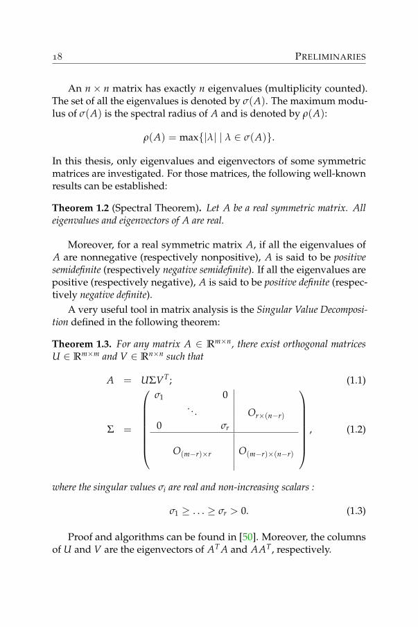
Theorem 1.2 (Spectral Theorem). Let A be a real symmetric matrix. Alleigenvalues and eigenvectors of A are real.
Moreover, for a real symmetric matrix A, if all the eigenvalues ofA are nonnegative (respectively nonpositive), A is said to be positivesemidefinite (respectively negative semidefinite). If all the eigenvalues arepositive (respectively negative), A is said to be positive definite (respec-tively negative definite).
A very useful tool in matrix analysis is the Singular Value Decomposi-tion defined in the following theorem:
Theorem 1.3. For any matrix A ∈ Rm×n, there exist orthogonal matricesU ∈ Rm×m and V ∈ Rn×n such that
A = UΣVT; (1.1)
Σ =
σ1 0. . . Or×(n−r)
0 σr
O(m−r)×r O(m−r)×(n−r)
, (1.2)
where the singular values σi are real and non-increasing scalars :
σ1 ≥ . . . ≥ σr > 0. (1.3)
Proof and algorithms can be found in [50]. Moreover, the columnsof U and V are the eigenvectors of AT A and AAT, respectively.
1.1 MATRIX THEORY AND LINEAR ALGEBRA
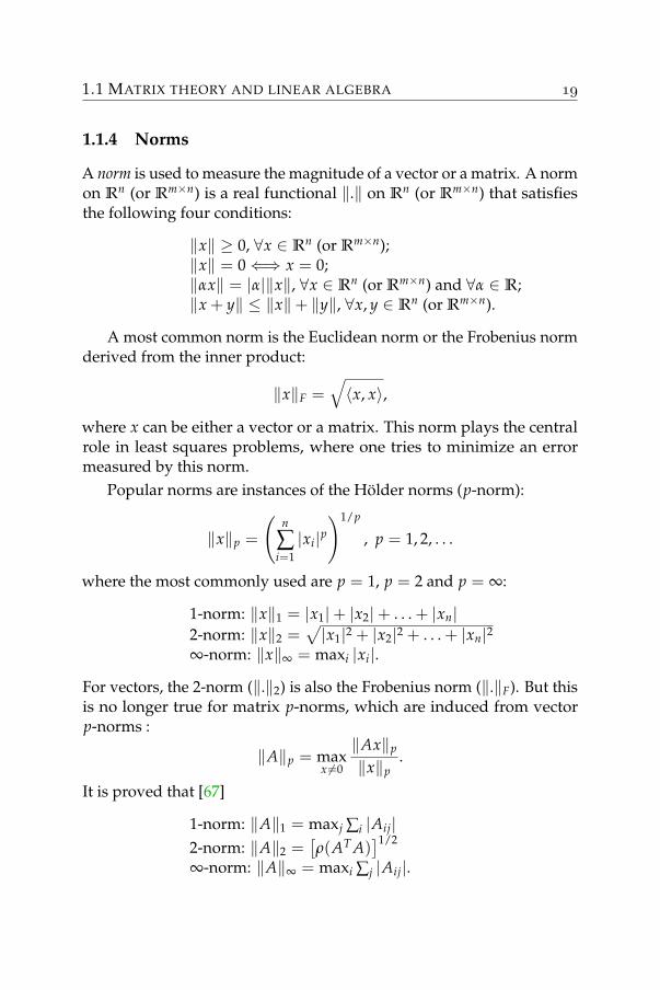
1.1.4 Norms
A norm is used to measure the magnitude of a vector or a matrix. A normon Rn (or Rm×n) is a real functional ‖.‖ on Rn (or Rm×n) that satisfiesthe following four conditions:
‖x‖ ≥ 0, ∀x ∈ Rn (or Rm×n);‖x‖ = 0⇐⇒ x = 0;‖αx‖ = |α|‖x‖, ∀x ∈ Rn (or Rm×n) and ∀α ∈ R;‖x + y‖ ≤ ‖x‖+ ‖y‖, ∀x, y ∈ Rn (or Rm×n).
A most common norm is the Euclidean norm or the Frobenius normderived from the inner product:
‖x‖F =√〈x, x〉,
where x can be either a vector or a matrix. This norm plays the centralrole in least squares problems, where one tries to minimize an errormeasured by this norm.
Popular norms are instances of the Hölder norms (p-norm):
‖x‖p =
(n
∑i=1|xi|p
)1/p
, p = 1, 2, . . .
where the most commonly used are p = 1, p = 2 and p = ∞:
1-norm: ‖x‖1 = |x1|+ |x2|+ . . . + |xn|2-norm: ‖x‖2 =
√|x1|2 + |x2|2 + . . . + |xn|2
∞-norm: ‖x‖∞ = maxi |xi|.
For vectors, the 2-norm (‖.‖2) is also the Frobenius norm (‖.‖F). But thisis no longer true for matrix p-norms, which are induced from vectorp-norms :
‖A‖p = maxx 6=0
‖Ax‖p
‖x‖p.
It is proved that [67]
1-norm: ‖A‖1 = maxj ∑i |Aij|2-norm: ‖A‖2 =
[ρ(AT A)
]1/2
∞-norm: ‖A‖∞ = maxi ∑j |Aij|.
PRELIMINARIES
Since the main problem treated in this thesis is a constrained leastsquares problem, the Frobenius norm will be extensively used. Othernorms will also be used to add more constraints on the main problem.
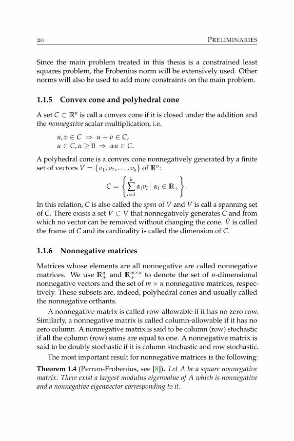
1.1.5 Convex cone and polyhedral cone
A set C ⊂ Rn is call a convex cone if it is closed under the addition andthe nonnegative scalar multiplication, i.e.
u, v ∈ C ⇒ u + v ∈ C,u ∈ C, α ≥ 0 ⇒ αu ∈ C.
A polyhedral cone is a convex cone nonnegatively generated by a finiteset of vectors V = v1, v2, . . . , vk of Rn:
C =
k
∑i=1
αivi | αi ∈ R+
.
In this relation, C is also called the span of V and V is call a spanning setof C. There exists a set V ⊂ V that nonnegatively generates C and fromwhich no vector can be removed without changing the cone. V is calledthe frame of C and its cardinality is called the dimension of C.
1.1.6 Nonnegative matrices
Matrices whose elements are all nonnegative are called nonnegativematrices. We use Rn
+ and Rm×n+ to denote the set of n-dimensional
nonnegative vectors and the set of m× n nonnegative matrices, respec-tively. These subsets are, indeed, polyhedral cones and usually calledthe nonnegative orthants.
A nonnegative matrix is called row-allowable if it has no zero row.Similarly, a nonnegative matrix is called column-allowable if it has nozero column. A nonnegative matrix is said to be column (row) stochasticif all the column (row) sums are equal to one. A nonnegative matrix issaid to be doubly stochastic if it is column stochastic and row stochastic.
The most important result for nonnegative matrices is the following:
Theorem 1.4 (Perron-Frobenius, see [8]). Let A be a square nonnegativematrix. There exist a largest modulus eigenvalue of A which is nonnegativeand a nonnegative eigenvector corresponding to it.
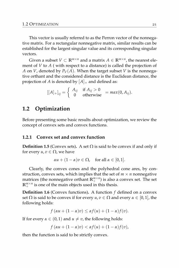
1.2 OPTIMIZATION
This vector is usually referred to as the Perron vector of the nonnega-tive matrix. For a rectangular nonnegative matrix, similar results can beestablished for the largest singular value and its corresponding singularvectors.
Given a subset V ⊂ Rm×n and a matrix A ∈ Rm×n, the nearest ele-ment of V to A ( with respect to a distance) is called the projection ofA on V, denoted by PV(A). When the target subset V is the nonnega-tive orthant and the considered distance is the Euclidean distance, theprojection of A is denoted by [A]+ and defined as:
[[A]+]ij =
Aij if Aij > 00 otherwise
= max(0, Aij).
1.2 Optimization
Before presenting some basic results about optimization, we review theconcept of convex sets and convex functions.
1.2.1 Convex set and convex function
Definition 1.5 (Convex sets). A set Ω is said to be convex if and only iffor every u, v ∈ Ω, we have
αu + (1− α)v ∈ Ω, for all α ∈ [0, 1].
Clearly, the convex cones and the polyhedral cone ares, by con-struction, convex sets, which implies that the set of m× n nonnegativematrices (the nonnegative orthant Rm×n
+ ) is also a convex set. The setRm×n
+ is one of the main objects used in this thesis.
Definition 1.6 (Convex functions). A function f defined on a convexset Ω is said to be convex if for every u, v ∈ Ω and every α ∈ [0, 1], thefollowing holds:
f (αu + (1− α)v) ≤ α f (u) + (1− α) f (v).
If for every α ∈ (0, 1) and u 6= v, the following holds:
f (αu + (1− α)v) < α f (u) + (1− α) f (v),
then the function is said to be strictly convex.
PRELIMINARIES
For more details about convex sets and convex functions, see [21].
1.2.2 Optimality conditions
Now, we summarize some basic results on the optimization problem
minx∈Ω
f (x),
where f is a real-valued function taken on the feasible set Ω ⊂ Rn.We distinguish two types of minima.
Definition 1.7 (Local minimum). A point x∗ ∈ Ω is said to be a localminimum of f over Ω if there exists an open neighborhood N(x∗) of x∗
such that for all x ∈ N(x∗) ∩Ω, f (x) ≥ f (x∗). It is considered a strictlocal minimum if for all x ∈ N(x∗) ∩Ω and x 6= x∗, f (x) > f (x∗).
Definition 1.8 (Global minimum). A point x∗ ∈ Ω is said to be a globalminimum of f over Ω if for all x ∈ Ω, f (x) ≥ f (x∗). A point x∗ ∈ Ω issaid to be a strict global minimum of f over Ω if for all x ∈ Ω, x 6= x∗,f (x) > f (x∗).
Usually, unless f has some convexity properties, finding the globalminimum is a very difficult task that needs global knowledge of thefunction f . On the other hand, finding local minima requires onlyknowledge of the neighborhood. The necessary conditions for localminima can also be easily derived by differential calculus. This explainswhy in our minimization problem we will try to find a local minimum,instead of a global one.
In order to set up necessary conditions satisfied by local minima,the basic idea is to look around a point using the concept of feasibledirections. From a point x ∈ Ω, a vector d is a feasible direction if thereis an α > 0 such that x + αd ∈ Ω for all α ∈ [0, α]. We have the followingfirst-order necessary conditions:
Proposition 1.9 ([87]). Let Ω be a subset of Rn and f be a continuouslydifferentiable function on Ω. If x∗ is a local minimum of f over Ω, then forevery feasible direction d at x∗, we have
(∇ f (x∗))Td ≥ 0. (1.4)
1.2 OPTIMIZATION
Conversely, every point that satisfies the condition (1.4) is called astationary point. When x∗ is an interior point of Ω, then every vector d isa feasible direction and (1.4) implies ∇ f (x∗) = 0.
If Ω is convex, to create all the feasible directions, one can use thevectors d = x− x∗, for every x ∈ Ω. This will generate all the feasibledirections at x∗, since from the convexity of Ω, we have
x∗ + αd = x∗ + α(x− x∗) = αx + (1− α)x∗ ∈ Ω, for all α ∈ [0, 1].
Therefore, a point x∗ is said to be a stationary point if it satisfies
(∇ f (x∗))T(x− x∗) ≥ 0, ∀x ∈ Ω.
For the special case where f and Ω are convex, every local minimumis also a global minimum. Furthermore, the set of all such minima isconvex. For more results and implications, see [87].
1.2.3 Karush-Kuhn-Tucker conditions
Let us consider the following constrained optimization problem:
minhi(x)=0gj(x)≤0
f (x),
where hi(x) = 0, (i = 1, . . . , k) are k equality constraints and gj(x) ≤ 0(j = 1, . . . , m) are m inequality constraints. The following is known asKarush-Kuhn-Tucker necessary conditions (or KKT conditions):
Proposition 1.10 ([13]). Let x∗ be the local minimum of the above problem.Suppose that f , hi and gj are continuously differentiable functions from Rn
to R and ∇hi(x∗) and ∇gj(x∗) are linearly independent. Then there existunique constants µi (i = 1, . . . , k) and λj (j = 1, . . . , m), such that:
∇ f (x∗) + ∑ki=1 µi∇hi(x∗) + ∑m
j=1 λj∇gj(x∗) = 0,λj ≥ 0, j = 1, . . . , mλjgj(x∗) = 0, j = 1, . . . , m.
This constrained problem is often written in its associated LagrangeFunction:
L(x, µi, . . . , µk, λ1, . . . , λm) = f (x) +k
∑i=1
µihi(x) +m
∑j=1
λjgj(x)
PRELIMINARIES
where µi (i = 1, . . . , k) and λj (j = 1, . . . , m) are the same as those in theKKT conditions and are called Lagrange multipliers.
1.2.4 Coordinate descent algorithm on a convex set
We briefly describe a method for solving the following problem
minx∈Ω
f (x),
where Ω ⊂ Rn is a Cartesian product of closed convex sets Ω1, Ω2, . . . ,Ωm, where Ωi ⊂ Rni (i = 1,. . . ,m) and ∑i ni = n. The variable x is alsopartitioned accordingly as
x =
x1...
xm
,
where xi ∈ Ωi. Algorithm 1 is called the coordinate descent algorithm.If we assume that Step 4 of Algorithm 1 can be solved exactly and
Algorithm 1 Coordinate descent
1: Initialize xi2: repeat3: for i = 1 to m do4: Solve xi = argminξ∈Ωi
f (x1, . . . , xi−1, ξ, xi+1, . . . , xm)5: end for6: until Stopping condition
the minimum is uniquely attained, then we have the following result.Because this result is extensively used in this thesis, we include here itsproof taken from Proposition 2.7.1 in [13].
Theorem 1.11 (Convergence of Coordinate Descent Method). Supposethat f is a continuously differentiable function over the set Ω described above.Furthermore, suppose that for each i and x ∈ Ω, the solution of
minξ∈Ωi
f (x1, . . . , xi−1, ξ, xi+1, . . . , xm)
is uniquely attained. Let xk be the sequence generated by Algorithm 1. Thenevery limit point is a stationary point.
1.2 OPTIMIZATION
Proof. Let
zki =
(xk+1
1 , . . . , xk+1i , xk
i+1, . . . , xkm
).
Step 4 of Algorithm 1 implies
f (xk) ≥ f (zk1) ≥ f (zk
2) ≥ · · · ≥ f (zkm−1) ≥ f (zk
m), ∀k. (1.5)
Let x = (x1, . . . , xm) be a limit point of the sequence xk. Notice thatx ∈ Ω because Ω is closed. Equation (1.5) implies that the sequence f (xk) converges to f (x). It now remains to show that x minimizes fover Ω.
Let xk j | j = 0, 1, . . . be a subsequence of xk that converges to x.
We first show that xk j+11 − x
k j1 converges to zero as j → ∞. Assume
the contrary or, equivalently, that zk j1 − xk j does not converges to zero.
Let γk j = ‖zk j1 − xk j‖. By possibly restricting to a subsequence of k j,
we may assume that there exists some γ > 0 such that γk j ≥ γ for all
j. Let sk j1 = (z
k j1 − xk j)/γk j . Thus, z
k j1 = xk j + γk j s
k j1 , ‖sk j
1 ‖ = 1, and sk j1
differs from zero only along the first block-component. Notice that sk j1
belongs to a compact set and therefore has a limit point s1. By restricting
to a further subsequence of k j, we assume that sk j1 converges to s1.
Let us fix some ε ∈ [0, 1]. Notice that 0 ≥ εγ ≥ γk j . Therefore,xk j + εγs
k j1 lies on the segment joining xk j and xk j + γk j s
k j1 = z
k j1 , and
belongs to Ω because Ω is convex. Using the fact that zk j1 minimizes f
over all x that differ from xk j along the first block-component, we obtain
f (zk j1 ) = f (xk j + γk j s
k j1 ) ≤ f (xk j + εγs
k j1 ) ≤ f (xk j).
Since f (xk j) converges to f (x), Equation (1.5) shows that f (zk j1 ) also
converges to f (x). We now take the limit as j tends to infinity, to obtainf (x) ≤ f (x + εγs1) ≤ f (x). We conclude that f (x) = f (x + εγs1), forevery ε ∈ [0, 1]. Since γs1 6= 0, this contradicts the hypothesis that fis uniquely minimized when viewed as a function of the first block-
component. This contradiction establishes that xk j+11 − x
k j1 converges to
zero. In particular, zk j1 converges to x.
PRELIMINARIES
From Step 4 of Algorithm 1, we have
f (zk j1 ) ≤ f (x1, x
k j2 , . . . , x
k jm), ∀x1 ∈ Ω1.
Taking the limit as j tends to infinity, we obtain
f (x) ≤ f (x1, xk j2 , . . . , x
k jm), ∀x1 ∈ Ω1.
Using Proposition 1.9 over the convex set Ω1, we conclude that
∇1 f (x)T(x1 − x1) ≥ 0, x1 ∈ Ω1,
where ∇i f denotes the gradient of f with respect to the component xi.
Let us now consider the sequence zk j1 . We have already shown
that zk j1 converges to x. A verbatim repetition of the preceding argument
shows that xk j+12 − x
k j2 converges to zero and ∇1 f (x)T(x1 − x1) ≥ 0, for
every x2 ∈ Ω2. Continuing inductively, we obtain ∇i f (x)T(xi − xi) ≥0, for every xi ∈ Ωi and for every i. Adding these inequalities, andusing the Cartesian product structure of the set Ω, we conclude that∇ f (x)(x− x) ≥ 0 for every x ∈ Ω.
1.3 Low-rank matrix approximation
Low-rank approximation is a special case of matrix nearness problem[58]. When only a rank constraint is imposed, the optimal approximationwith respect to the Frobenius norm can be obtained from the SingularValue Decomposition.
We first investigate the problem without the nonnegativity constrainton the low-rank approximation. This is useful for understanding prop-erties of the approximation when the nonnegativity constraints areimposed but inactive. We begin with the well-known Eckart-YoungTheorem.
Theorem 1.12 (Eckart-Young). Let A ∈ Rm×n (m ≥ n) have the singular
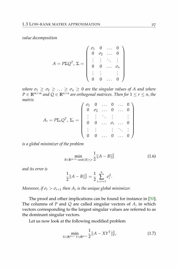
1.3 LOW-RANK MATRIX APPROXIMATION
value decomposition
A = PΣQT, Σ =
σ1 0 . . . 00 σ2 . . . 0...
.... . .
...0 0 . . . σn...
......
0 0 . . . 0
where σ1 ≥ σ2 ≥ . . . ≥ σn ≥ 0 are the singular values of A and whereP ∈ Rm×m and Q ∈ Rn×n are orthogonal matrices. Then for 1 ≤ r ≤ n, thematrix
Ar = PΣrQT, Σr =
σ1 0 . . . 0 . . . 00 σ2 . . . 0 . . . 0...
.... . .
......
0 0 . . . σr . . . 0...
......
. . ....
0 0 . . . 0 . . . 0
is a global minimizer of the problem
minB∈Rm×n rank(B)≤r
12‖A− B‖2
F (1.6)
and its error is12‖A− B‖2
F =12
n
∑i=r+1
σ2i .
Moreover, if σr > σr+1 then Ar is the unique global minimizer.
The proof and other implications can be found for instance in [50].The columns of P and Q are called singular vectors of A, in whichvectors corresponding to the largest singular values are referred to asthe dominant singular vectors.
Let us now look at the following modified problem
minX∈Rm×r Y∈Rn×r
12‖A− XYT‖2
F, (1.7)
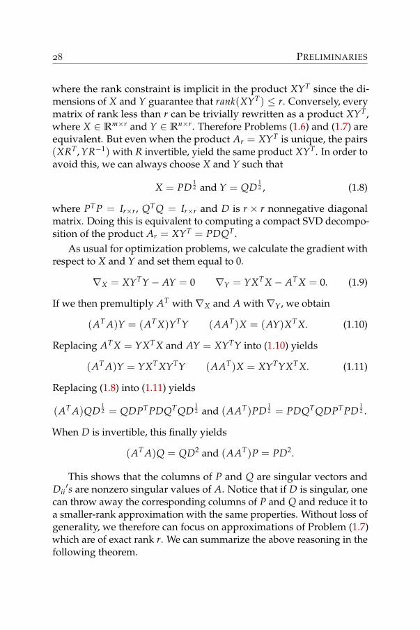
PRELIMINARIES
where the rank constraint is implicit in the product XYT since the di-mensions of X and Y guarantee that rank(XYT) ≤ r. Conversely, everymatrix of rank less than r can be trivially rewritten as a product XYT,where X ∈ Rm×r and Y ∈ Rn×r. Therefore Problems (1.6) and (1.7) areequivalent. But even when the product Ar = XYT is unique, the pairs(XRT, YR−1) with R invertible, yield the same product XYT. In order toavoid this, we can always choose X and Y such that
X = PD12 and Y = QD
12 , (1.8)
where PTP = Ir×r, QTQ = Ir×r and D is r × r nonnegative diagonalmatrix. Doing this is equivalent to computing a compact SVD decompo-sition of the product Ar = XYT = PDQT.
As usual for optimization problems, we calculate the gradient withrespect to X and Y and set them equal to 0.
∇X = XYTY− AY = 0 ∇Y = YXTX− ATX = 0. (1.9)
If we then premultiply AT with ∇X and A with ∇Y, we obtain
(AT A)Y = (ATX)YTY (AAT)X = (AY)XTX. (1.10)
Replacing ATX = YXTX and AY = XYTY into (1.10) yields
(AT A)Y = YXTXYTY (AAT)X = XYTYXTX. (1.11)
Replacing (1.8) into (1.11) yields
(AT A)QD12 = QDPTPDQTQD
12 and (AAT)PD
12 = PDQTQDPTPD
12 .
When D is invertible, this finally yields
(AT A)Q = QD2 and (AAT)P = PD2.
This shows that the columns of P and Q are singular vectors andDii′s are nonzero singular values of A. Notice that if D is singular, one
can throw away the corresponding columns of P and Q and reduce it toa smaller-rank approximation with the same properties. Without loss ofgenerality, we therefore can focus on approximations of Problem (1.7)which are of exact rank r. We can summarize the above reasoning in thefollowing theorem.
1.3 LOW-RANK MATRIX APPROXIMATION
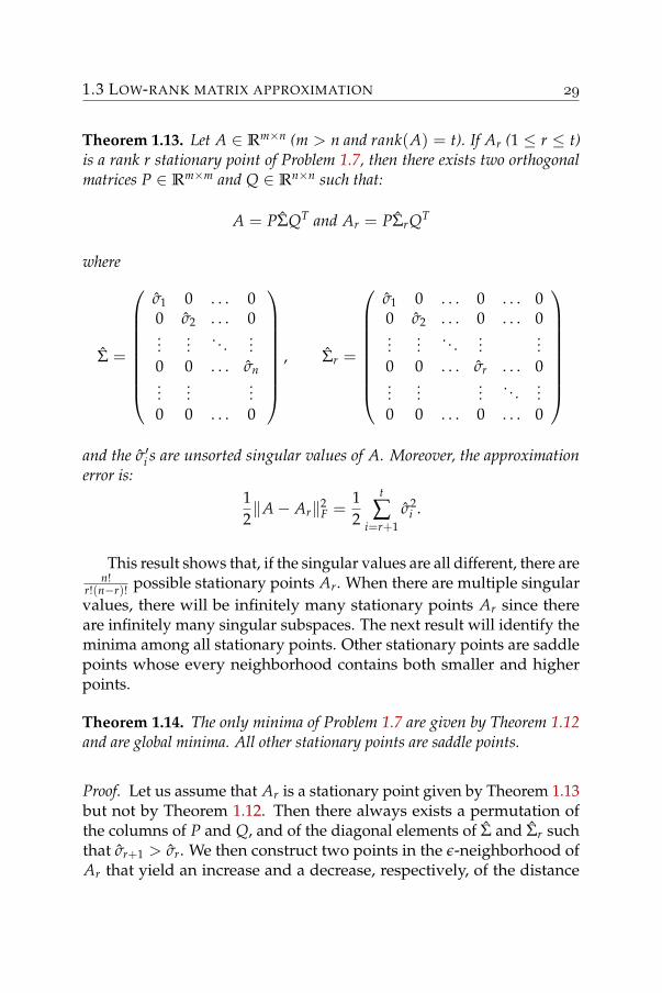
Theorem 1.13. Let A ∈ Rm×n (m > n and rank(A) = t). If Ar (1 ≤ r ≤ t)is a rank r stationary point of Problem 1.7, then there exists two orthogonalmatrices P ∈ Rm×m and Q ∈ Rn×n such that:
A = PΣQT and Ar = PΣrQT
where
Σ =
σ1 0 . . . 00 σ2 . . . 0...
.... . .
...0 0 . . . σn...
......
0 0 . . . 0
, Σr =
σ1 0 . . . 0 . . . 00 σ2 . . . 0 . . . 0...
.... . .
......
0 0 . . . σr . . . 0...
......
. . ....
0 0 . . . 0 . . . 0
and the σ′i s are unsorted singular values of A. Moreover, the approximationerror is:
12‖A− Ar‖2
F =12
t
∑i=r+1
σ2i .
This result shows that, if the singular values are all different, there aren!
r!(n−r)! possible stationary points Ar. When there are multiple singularvalues, there will be infinitely many stationary points Ar since thereare infinitely many singular subspaces. The next result will identify theminima among all stationary points. Other stationary points are saddlepoints whose every neighborhood contains both smaller and higherpoints.
Theorem 1.14. The only minima of Problem 1.7 are given by Theorem 1.12and are global minima. All other stationary points are saddle points.
Proof. Let us assume that Ar is a stationary point given by Theorem 1.13but not by Theorem 1.12. Then there always exists a permutation ofthe columns of P and Q, and of the diagonal elements of Σ and Σr suchthat σr+1 > σr. We then construct two points in the ε-neighborhood ofAr that yield an increase and a decrease, respectively, of the distance
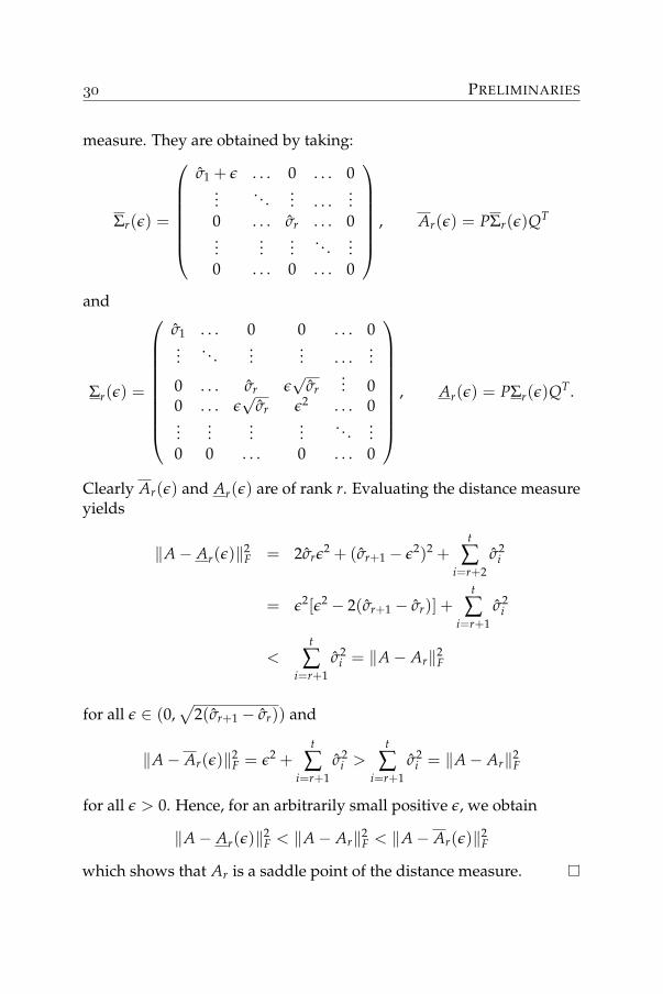
PRELIMINARIES
measure. They are obtained by taking:
Σr(ε) =
σ1 + ε . . . 0 . . . 0
.... . .
... . . ....
0 . . . σr . . . 0...
......
. . ....
0 . . . 0 . . . 0
, Ar(ε) = PΣr(ε)QT
and
Σr(ε) =
σ1 . . . 0 0 . . . 0...
. . ....
... . . ....
0 . . . σr ε√
σr... 0
0 . . . ε√
σr ε2 . . . 0...
......
.... . .
...0 0 . . . 0 . . . 0
, Ar(ε) = PΣr(ε)QT.
Clearly Ar(ε) and Ar(ε) are of rank r. Evaluating the distance measureyields
‖A− Ar(ε)‖2F = 2σrε2 + (σr+1 − ε2)2 +
t
∑i=r+2
σ2i
= ε2[ε2 − 2(σr+1 − σr)] +t
∑i=r+1
σ2i
<t
∑i=r+1
σ2i = ‖A− Ar‖2
F
for all ε ∈ (0,√
2(σr+1 − σr)) and
‖A− Ar(ε)‖2F = ε2 +
t
∑i=r+1
σ2i >
t
∑i=r+1
σ2i = ‖A− Ar‖2
F
for all ε > 0. Hence, for an arbitrarily small positive ε, we obtain
‖A− Ar(ε)‖2F < ‖A− Ar‖2
F < ‖A− Ar(ε)‖2F
which shows that Ar is a saddle point of the distance measure.

1.3 LOW-RANK MATRIX APPROXIMATION
When we add a nonnegativity constraint in the next section, theresults of this section will help to identify stationary points at which allthe nonnegativity constraints are inactive.

PRELIMINARIES
2
NONNEGATIVE MATRIXFACTORIZATION
This chapter is a presentation of the Nonnegative Matrix Factorizationproblem. It consists of the formulation of the problem, the descriptionof the solutions and some observations. It gives the basics for the restof this thesis. Some observations are studied more carefully in otherchapters.
One could argue that the name Nonnegative Matrix Factorizationmaybe misleading in some cases and that Nonnegative Matrix Ap-proximation should be used instead. The term “Factorization” maybeunderstood as an exact decomposition such as Cholesky decomposition,LU decomposition, etc. where the input matrix is exactly factorizedas a product of other matrices. However, “Nonnegative Matrix Factor-ization” has become so popular that it does stand for the problem ofapproximating a nonnegative matrix by a product of two nonnegativematrices. We continue to use this term and refer to Exact NonnegativeMatrix Factorization for the exact case.
2.1 Problem statement
Nonnegative Matrix Factorization was first introduced by Paatero andTapper in [97]. But it has gained popularity by the works of Lee andSeung [80]. They argue that the nonnegativity is important in humanperceptions and also give two simple algorithms for finding a nonnega-tive representation for nonnegative data. Given an m× n nonnegative
NONNEGATIVE MATRIX FACTORIZATION
matrix A (i.e. Aij ≥ 0) and a reduced rank r (r < min(m, n)), the nonneg-ative matrix factorization problem consists in finding two nonnegativematrices U ∈ Rm×r
+ and V ∈ Rn×r+ that approximate A, i.e.
A ≈ UVT.
Looking at the columns of A, one sees that each of them is approxi-mated by a conic combination of r nonnegative basis vectors that are thecolumns of U
A:i ≈r
∑j=1
VijU:j.
We can consider the columns of U as the basis of the cone U completelycontained inside the nonnegative orthant. And each column of A isapproximated by an element of U, typically the closest element to thecolumn. We can also exchange the role of U and V to point out thateach row of A is approximated by an element of V, typically the closestelement to the row, where V is the cone generated by the column of V.
There are several ways to quantify the difference between the datamatrix A and the model matrix UVT. But the most used measure is theFrobenius norm:
F(A, UVT) =12‖A−UVT‖2
F =12
m
∑i=1
n
∑i=1
(Aij − [UVT]ij
)2
which is also referred to as the Euclidean Distance.Suppose that U is fixed, the function F(U, V) = 1
2‖A−UVT‖2F can
be seen as a composition of the Frobenius norm and a linear transforma-tion of V. Therefore, F is convex in V. Likewise, if V is fixed, F is convexon U.
Throughout this thesis, the nonnegative matrix factorization problemwill be studied with a bias to the Frobenius norm. The main problem isthe following:
Problem 2.1 (Nonnegative matrix factorization - NMF). Given a m× nnonnegative matrix A and an integer r < min(m, n), solve
minU∈Rm×r
+ V∈Rn×r+
12‖A−UVT‖2
F.
2.1 PROBLEM STATEMENT
Where r is called the reduced rank. From now on, m and n will beused to denote the size of the target matrix A and r is the reduced rankof a factorization.
We rewrite the nonnegative matrix factorization as a standard non-linear optimization problem:
min−U≤0 −V≤0
12‖A−UVT‖2
F.
The associated Lagrangian function is
L(U, V, µ, ν) =12‖A−UVT‖2
F − µ U − ν V,
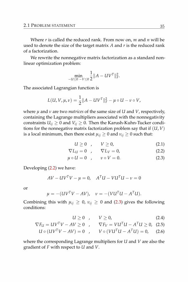
where µ and ν are two matrices of the same size of U and V, respectively,containing the Lagrange multipliers associated with the nonnegativityconstraints Uij ≥ 0 and Vij ≥ 0. Then the Karush-Kuhn-Tucker condi-tions for the nonnegative matrix factorization problem say that if (U, V)is a local minimum, then there exist µij ≥ 0 and νij ≥ 0 such that:
U ≥ 0 , V ≥ 0, (2.1)∇LU = 0 , ∇LV = 0, (2.2)µ U = 0 , ν V = 0. (2.3)
Developing (2.2) we have:
AV −UVTV − µ = 0, ATU −VUTU − ν = 0
orµ = −(UVTV − AV), ν = −(VUTU − ATU).
Combining this with µij ≥ 0, νij ≥ 0 and (2.3) gives the followingconditions:
U ≥ 0 , V ≥ 0, (2.4)∇FU = UVTV − AV ≥ 0 , ∇FV = VUTU − ATU ≥ 0, (2.5)
U (UVTV − AV) = 0 , V (VUTU − ATU) = 0, (2.6)
where the corresponding Lagrange multipliers for U and V are also thegradient of F with respect to U and V.
NONNEGATIVE MATRIX FACTORIZATION
Since the Euclidean distance is not convex with respect to both vari-ables U and V at the same time, these conditions are only necessary. Thisis implied because of the existence of saddle points and maxima. Wethen call all the points that satisfy the above conditions, the stationarypoints.
Definition 2.2 (NMF stationary point). We call (U, V) a stationary pointof the NMF Problem if and only if U and V satisfy the KKT conditions(2.4), (2.5) and (2.6).
Alternatively, a stationary point (U, V) of the NMF problem can alsobe defined by using the condition in Proposition 1.9 on the convex setsRm×r
+ and Rn×r+ , that is⟨(
∇FU∇FV
),(
X−UY−V
)⟩≥ 0, ∀ X ∈ Rm×r
+ , Y ∈ Rn×r+ , (2.7)
which can be shown to be equivalent to the KKT conditions (2.4), (2.5)and (2.6). Indeed, it is trivial that the KKT conditions imply (2.7). Andby carefully choosing different values of X and Y from (2.7), one caneasily prove that the KKT conditions hold.
Representing a rank-k matrix by the product UVT is, in fact, rarelyused due to the loss of the uniqueness of the presentation. Because anonnegative factorization is, by definition, in this form, the rest of thesection tries to fix the uniqueness problem and to establish some simplerelations between the approximations.
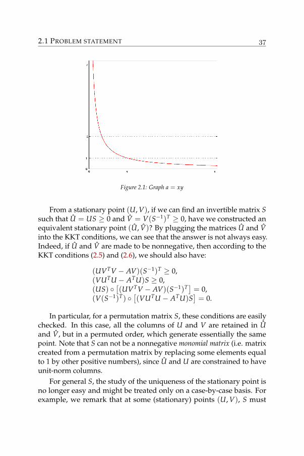
Let us consider the simplest nonnegative factorization problemwhere the matrix A is just a scalar a. The problem (of rank one) isthen to find two scalar x and y whose product approximate a. Prob-lem 2.1 admits only exact approximations (a− xy)2 = 0, and we haveinfinite number of solutions given by the graph xy = a (Figure 2.1).
If we impose the unit norm condition on x (i.e. ‖x‖ = 1), then forthis particular case, there will be only one solution (x = 1 and y = a).
To extend this scaling technique to higher dimensions, we continueto constrain the first factor U to have unit-norm columns. But this nolonger guarantees the uniqueness of the approximations. Moreover, it isnot easy to determine when and how the uniqueness is obtainable.
Two approximations (U1, V1) and (U2, V2) are said to be equivalentiff they yield the same product, i.e. U1VT
1 = U2VT2 .
2.1 PROBLEM STATEMENT
Figure 2.1: Graph a = xy
From a stationary point (U, V), if we can find an invertible matrix Ssuch that U = US ≥ 0 and V = V(S−1)T ≥ 0, have we constructed anequivalent stationary point (U, V)? By plugging the matrices U and Vinto the KKT conditions, we can see that the answer is not always easy.Indeed, if U and V are made to be nonnegative, then according to theKKT conditions (2.5) and (2.6), we should also have:
(UVTV − AV)(S−1)T ≥ 0,(VUTU − ATU)S ≥ 0,(US)
[(UVTV − AV)(S−1)T] = 0,
(V(S−1)T) [(VUTU − ATU)S
]= 0.
In particular, for a permutation matrix S, these conditions are easilychecked. In this case, all the columns of U and V are retained in Uand V, but in a permuted order, which generate essentially the samepoint. Note that S can not be a nonnegative monomial matrix (i.e. matrixcreated from a permutation matrix by replacing some elements equalto 1 by other positive numbers), since U and U are constrained to haveunit-norm columns.
For general S, the study of the uniqueness of the stationary point isno longer easy and might be treated only on a case-by-case basis. Forexample, we remark that at some (stationary) points (U, V), S must
NONNEGATIVE MATRIX FACTORIZATION
be a permutation matrix, otherwise, the nonnegativity of (U, V) willnot be met. This implies that we can not generate other equivalentapproximations. The following result helps to identify a class of them.
Lemma 2.3. If U and V both contain a r× r monomial matrix, then S canonly be the permutation matrices.
Proof. The assumption implies that we can select r rows of U to form anr× r monomial matrix Ur and r rows of V to form an r× r monomialmatrix Vr. Then the nonnegativity constraint implies
UrS ≥ 0 and Vr(S−1)T ≥ 0.
Since, Ur and Vr are nonnegative monomial matrices, both S and S−1
must be nonnegative. This is only possible when S is a monomial ma-trix1. Moreover, U and US are constrained to have unit-norm columns,S can only be permutation matrices.
Another way to consider the set of equivalent stationary points isto identify them by all the possible exact factorization of the matrixA = UVT where (U, V) is one known entry of the set. But there is noeasy method to construct this set.
A better representation of the stationary point is similar to the singu-lar value decomposition. We can use a triplet (U, D, V) to represent aNMF stationary point. So, instead of solving Problem 2.1, we solve thefollowing problem:
(u∗i , d∗i , v∗i )ri=1 = argmin
ui≥0 uTi ui=1
vi≥0 vTi vi=1
di≥0
‖A−r
∑i=1
diuivTi ‖2
2,
1We have S ≥ 0 and S−1 ≥ 0 and the off-diagonal elements of SS−1 = Ir andS−1S = Ir are zero. As a consequence, if Sij > 0, we can conclude that S−1
jk = 0 and
S−1li = 0 for k 6= i and l 6= j. Because S−1 is invertible hence can not contain zero
rows and columns, S−1ji is the only positive element on the jth row and ith column of
S−1. Reciprocally, S−1ji > 0 implies Sij is the only positive element on the ith row and
jth column of S. Since S can not contain zero rows and columns, repeating the abovereasoning through all the nonzero elements of S yields the desired result.
2.2 SOLUTION
or in matrix representation, U and V is nonnegative matrices with unit-norm columns and D is a nonnegative diagonal matrix. The matrixA is then approximated by UDVT. With this, we can also sort thecomponents in decreasing order of the value of Dii (i.e. D11 ≥ D22 ≥· · · ≥ Drr). This helps to compare equivalent solutions.
In Chapter 4, we use this representation to design our iterative algo-rithm and point out its advantages.
2.2 Solution
There are two values of reduced rank r for which we can trivially identifythe global solution which are r = 1 and r = min(m, n). For r = 1, apair of dominant singular vectors are a global minimizer. And forr = min(m, n), (U = A, V = I) is a global minimizer. Since most ofexisting methods for the nonnegative matrix factorization are descentalgorithms, we should pay attention to all local minimizers. For therank-one case, they can easily be characterized.
2.2.1 Rank one case
The rank-one NMF problem of a nonnegative matrix A can be rewrittenas
minu∈Rm
+ v∈Rn+
12‖A− uvT‖2
F (2.8)
and a complete analysis can be carried out. It is well known that anypair of nonnegative Perron vectors of AAT and AT A yields a globalminimizer of this problem, but we can also show that the only stationarypoints of (2.8) are given by such vectors. The following theorem excludesthe case where u = 0 and/or v = 0.
Theorem 2.4. The pair (u, v) is a local minimizer of (2.8) if and only if u andv are nonnegative eigenvectors of AAT and AT A respectively of the eigenvalueσ = ‖u‖2
2‖v‖22.
Proof. The if part easily follows from Theorem 1.13. For the only if partwe proceed as follows. Without loss of generality, we can permute therows and columns of A such that the corresponding vectors u and v

NONNEGATIVE MATRIX FACTORIZATION
are partitioned as (u+ 0)T and (v+ 0)T respectively, where u+, v+ > 0.Partition the corresponding matrix A conformably as follows
A =(
A11 A12A21 A22
),
then from (2.5) we have(u+vT
+ 00 0
)(v+0
)−(
A11 A12A21 A22
)(v+0
)≥ 0
and (v+uT
+ 00 0
)(u+0
)−(
AT11 AT
21AT
12 AT22
)(u+0
)≥ 0
implying that A21v+ ≤ 0 and AT12u+ ≤ 0. Since A21 , A12 ≥ 0 and
u+, v+ > 0, we can conclude that A12 = 0 and A21 = 0. Then from (2.6)we have:
u+ (‖v+‖22u+ − A11v+) = 0 and v+ (‖u+‖2
2v+ − A+11u+) = 0.
Since u+, v+ > 0, we have:
‖v+‖22u+ = A11v+ and ‖u+‖2
2v+ = AT11u+
or
‖u+‖22‖v+‖2
2u+ = A11AT11u+ and ‖u+‖2
2‖v+‖22v+ = AT
11A11v+.
Setting σ = ‖u+‖22‖v+‖2
2 and using the block diagonal structure of Ayields the desired result.
Theorem 2.4 guarantees that all stationary points of the rank-onecase are nonnegative singular vectors of a submatrix of A. These resultsimply that a global minimizer of the rank-one NMF can be calculatedcorrectly based on the largest singular value and corresponding singularvectors of the matrix A.
For ranks other than 1 and min(m, n), there are no longer trivialstationary points. In the next section, we try to derive some simple char-acteristics of the local minima of the nonnegative matrix factorization.
2.2 SOLUTION
2.2.2 Characteristics of local minima
The KKT conditions (2.6) help to characterize the stationary points of theNMF problem. Summing up all the elements of one of the conditions(2.6), we get:
0 = ∑ij
(U (UVTV − AV)
)ij
=⟨
U, UVTV − AV⟩
=⟨
UVT, UVT − A⟩
. (2.9)
From that, we have some simple characteristics of the NMF solutions:
Theorem 2.5. Let (U, V) be a stationary point of the NMF problem, thenUVT ∈ B
( A2 , 1
2‖A‖F), the ball centered at A
2 and with radius = 12‖A‖F.
Proof. From (2.9) it immediately follows that⟨A2−UVT,
A2−UVT
⟩=⟨
A2
,A2
⟩which implies
UVT ∈ B(
A2
,12‖A‖F
).
Theorem 2.6. Let (U, V) be a stationary of the NMF problem, then
12‖A−UVT‖2
F =12(‖A‖2
F − ‖UVT‖2F)
.
Proof. From (2.9), we have⟨UVT, A
⟩=⟨UVT, UVT⟩. Therefore,
12
⟨A−UVT, A−UVT
⟩=
12(‖A‖2
F − 2⟨
UVT, A⟩
+ ‖UVT‖2F)
=12(‖A‖2
F − ‖UVT‖2F).
NONNEGATIVE MATRIX FACTORIZATION
Theorem 2.6 also suggests that at a stationary point (U, V) of theNMF problem, we should have ‖A‖2
F ≥ ‖UVT‖2F. This norm inequality
can be also found in [25] for less general cases where we have ∇FU = 0and ∇FV = 0 at a stationary point. For this particular class of NMFstationary point, all the nonnegativity constraints on U and Vare inac-tive. And all such stationary points are also stationary points of theunconstrained problem, characterized by Theorem 1.13.
We have seen in Theorem 1.13 that, for the unconstrained least-square problem the only stable stationary points are in fact global min-ima. Therefore, if the stationary points of the constrained problem areinside the nonnegative orthant (i.e. all constraints are inactive), we canthen probably reach the global minimum of the NMF problem. This canbe expected because the constraints may no longer prohibit the descentof the update.
The equality of ‖A‖2F ≥ ‖UVT‖2
F implied by Theorem 2.6 is onlyobtained when we have an exact factorization (i.e A = UVT) and it willbe the subject of the next section.
Let Ar be the optimal rank-r approximation of a nonnegative matrixA, which we obtain from the singular value decomposition, as indicatedin Theorem 1.13. Then we can easily construct its nonnegative part[Ar]+, which is obtained from Ar by just setting all its negative elementsequal to zero. This is in fact the closest matrix in the cone of nonnegativematrices to the matrix Ar, in the Frobenius norm (in that sense, it isits projection on that cone). We now derive some bounds for the error‖A− [Ar]+‖F.
Theorem 2.7. Let Ar be the best rank r approximation of a nonnegative matrixA, and let [Ar]+ be its nonnegative part, then
‖A− [Ar]+‖F ≤ ‖A− Ar‖F.
Proof. This follows easily from the convexity of the cone of nonnegativematrices. Since both A and [Ar]+ are nonnegative and since [Ar]+ is theclosest matrix in that cone to Ar we immediately obtain the inequality
‖A− Ar‖2F ≥ ‖A− [Ar]+‖2
F + ‖Ar − [Ar]+‖2F ≥ ‖A− [Ar]+‖2
F
from which the result readily follows.
2.3 EXACT FACTORIZATION AND NONNEGATIVE RANK
If we now compare this bound with the nonnegative approximationsthen we obtain the following inequalities. Let U∗VT
∗ be an optimalnonnegative rank r approximation of A and let UVT be any stationarypoint of the KKT conditions for a nonnegative rank r approximation,then we have :
‖A− [Ar]+|2F ≤ ‖A− Ar‖2F =
n
∑i=r+1
σ2i ≤ ‖A−U∗VT
∗ ‖2F ≤ ‖A−UVT‖2
F.
2.3 Exact factorization and nonnegative rank
In this section, we will take a brief look at a stricter problem wherewe are interested only in the solutions where the objective functionis zero. This means that the matrix A is exactly factorized by UVT
(i.e. A = UVT) with the same nonnegativity constraints on the factors.The smallest value of r, the inner rank of the factorization UVT, thatfactorizes correctly A is called the nonnegative rank of A, denoted byrank+
UVT (A). In [33], a nice treatment of the problem is carried out.The existence of an exact factorization of inner rank r is equivalent
to determining rank+UVT (A). For any r > rank+
UVT (A), we can triviallyconstruct an exact nonnegative factorization from the factorization UVT
of inner rank r by adding zero columns to the factors U and V.For the nonnegative rank, the following results are well known and
can be found in [33]. First, an upper bound and a lower bound of thisnumber are easily computed.
Lemma 2.8. Let A ∈ Rm×n+ . Then
rank(A) ≤ rank+UVT (A) ≤ min(m, n).
Proof. Since we can not construct the same matrix with lower rank thenthe first inequality holds. The second comes from one of the trivialfactorizations Im A and AIn.
In certain cases, the first equality holds. For the rank-one nonnega-tive matrix A, we know that it can be represented by uvT, where u andv are nonnegative. This implies that rank+
UVT (A) = rank(A) = 1. It isstill true for a rank-two matrix, which is proved in [33] and [3].
NONNEGATIVE MATRIX FACTORIZATION
Lemma 2.9. Let A ∈ Rm×n+ where rank(A) = 2. Then
rank+UVT (A) = 2.
Proof. Since A ≥ 0, the cone spanned by the columns of A is a con-vex polyhedral cone contained in the nonnegative orthant. Moreover,rank(A) = 2 implies that the cone is contained in a two dimensionallinear subspace. Therefore its spanning set, i.e. the columns of A, can bereduced to only two vectors called u1 and u2. Every column of A is thenrepresented by
A:i = V1iu1 + V2iu2, with V1i, V2i ≥ 0.
Creating U = (u1 u2) and V = Vij gives the desired rank-two non-negative factorization UVT.
The two spanning vectors u1 and u2 in the proof of the precedinglemma are indeed a pair of columns of A that has the largest anglebetween them, i.e.
(u1 u2) = argminA:i A:j
AT:i A:j
‖A:i‖‖A:j‖.
V is computed by solving a least square, which yields
V = ATU(UTU)−1 ≥ 0.
So far, we have seen that when rank(A) is 1, 2 or min(m, n), we canconstruct an exact nonnegative matrix factorization with the same rank.For matrices with other ranks, determining the nonnegative rank is verydifficult. Indeed, Vavasis in [121] has recently proved the NP-hardnessof the nonnegative matrix factorization. Therefore, all algorithms forsolving the exact problem are expected to have a non polynomial com-plexity. In [116], a method is proposed to create nonnegative matrixfactorization via extremal polyhedral cones. Another possibility is usingthe quantifier elimination algorithms [113] to check for the feasibility offactoring a nonnegative matrix A by a nonnegative factorization of innerrank less than r. All these algorithms are finite. One such algorithm isgiven by Renegar [101] and was used in the nonnegative rank problem
2.3 EXACT FACTORIZATION AND NONNEGATIVE RANK
in [33]. Recently, the same method has been applied to the completelypositive rank [9] (cfr. Chapter 7). This method is quite generic and canbe applied to other factorizations in this thesis. Here, we describe brieflyhow to derive the computational complexity bound for a nonnegativefactorization.
Consider a first-order formula over the reals having the form
(Q1x[1] ∈ Rn1) . . . (Qωx[ω] ∈ Rnω )P(y, x[1], . . . , x[ω]), (2.10)
where the quantifiers Qk ∈ ∀, ∃, the vector y contains n0 free variables(unquantified) and P is a boolean function constructed from M atomtrue-false expressions
gi(y, x[1], . . . , x[ω]) ∆i 0, i = 1, . . . , M
with gi are polynomials of degree less than d and comparison operators∆i ∈ <,≤, =, 6=,≥, >. Then the Renegar algorithm requires at most(Md)2O(ω) ∏k nk multiplications and additions and at most (Md)O(∑k nk)
evaluations of P.These complexity bounds are derived from the known constants ω,
n0, n1, M and d that can be easily computed for the standard nonnegativematrix factorization in the following lemma.
Lemma 2.10 ([101]). The Renegar algorithm requires at most (6mn)2O(1)m2n2
multiplications and additions and at most (6mn)O(mn) evaluations of P todetermine the feasibility of factorizing A by a nonnegative factorization UVT
of inner rank r.
Proof. We need to eliminate the quantifiers of the following formula:((UT, VT) ∈ Rr×(m+n)
)P(A, (UT, VT))
where P(A, (UT, VT)) =∧ij
(∑
kUikVjk = Aij
) ∧(∧ik
(Uik ≥ 0)
)∧
∧jk
(Vjk ≥ 0
) .
This configuration gives: ω = 1, n0 = mn, n1 = r(m + n) ≤ 2mn,M = mn + r(m + n) ≤ 3mn and d = 2. And the bounds follow.
NONNEGATIVE MATRIX FACTORIZATION
The result implies that the problem of determining the nonnega-tive rank can be solved in finite time by looping through r = 1, 2, . . . ,min(m, n), since the upper bound of the nonnegative rank is min(m, n).
The above lemma can be easily extended for other nonnegative ma-trix factorizations such as: multilayer nonnegative matrix factorizationand nonnegative tensor matrix factorization in the next section, sym-metric and semi-symmetric matrix factorization in Chapter 7. For eachproblem, ω = 1, n0 is equal to the number of elements of the targetmatrix (or tensor), n1 is the total number of elements of all the factors,M = n0 + n1 and d is equal to the number of factors. Simple countingsthen yield upper complexity bounds for Renegar algorithm for eachfeasibility problem.
Similar to the nonnegative rank, the completely-positive rank(rankUUT (A)) and the semi-symmetric nonnegative rank (rankUSUT (A))(crf. Chapter 7) can be also computed in finite time using the Renegaralgorithm. This is due to the existence of an upper bound on these ranks.
2.4 Extensions of nonnegative matrix factorization
The essence of the nonnegative matrix factorization is to represent non-negative data by a nonnegative combination of nonnegative basis vec-tors, usually called parts. To enlarge the representing capability of themethod, improvements are made on how these bases are combined andon the structure of the bases. More specifically, in the standard non-negative matrix factorization, each data vector A:j ∈ Rn
+ is representedby
A:j = ∑i
VjiU:i, with Vji ∈ R+ and U:i ∈ Rn+.
We can list here two constructions of U:i that may improve the perfor-mance of the nonnegative matrix factorization.
2.4.1 Multilayer nonnegative matrix factorization
We can assume that the U:i is approximated based on another set ofbases X:t. Again, each U:i is constructed by a nonnegative combinationof X:i’s. So we can write
U ≈ XX1
2.4 EXTENSIONS OF NONNEGATIVE MATRIX FACTORIZATION
where X and X1 are nonnegative. With the same reasoning, one canassume that X:i’s are not the primitives and constructed by another setof bases [X1]:i’s, and so on. This gives the formulation of the multilayernonnegative matrix factorization:
Problem 2.11 (Multilayer nonnegative matrix factorization).
minXi≥0 V≥0
12‖A− X0X1 . . . XkVT‖2
F,
where A is the nonnegative data matrix and V and Xi’s are nonnegativematrices of compatible sizes.
This problem was studied in a number of works, e.g. [36], [29].Another related problem is the Archetypal Analysis [35], where the aboveproblem is restricted to only three layers, wherein the first layer consistsof the data themselves. Each data column is approximated by a convexcombination of a set of archetypes that are, in turn, convex combinationsof the data columns. The problem to be solved is the following:
minX≥0 V≥0
XT1=1 V1=1
12‖A− (AX)VT‖2
F,
where each column of AX is an archetype.For the multilayer nonnegative matrix factorization, one can use
algorithms proposed in [36], [29] or the algorithm proposed in Section4.6.1 to construct an approximation.
2.4.2 Nonnegative Tensor Factorization
Data is, by its nature, not only restricted to nonnegative vectors, i.e. one-dimensional data. Each data can also be points in higher dimensions,for example m× n nonnegative matrices. And the additional model canbe adapted to handle such data
Aj ≈∑i
VjiUi,
where Vji ≥ 0 and Aj, Ui’s ∈ Rm×n+ .
NONNEGATIVE MATRIX FACTORIZATION
If we further restricted Ui’s to a nonnegative combination of somerank-one nonnegative matrices represented by xjyT
j where xj ∈ Rm+ and
yj ∈ Rn+. Then the problem of finding xj, yj and Vij from Ai’s is an
example of the following Nonnegative Tensor Factorization problem:
Problem 2.12 (Nonnegative Tensor Factorization).
minuij∈R
ni+
12‖A−
r
∑j=1
u1j ? u2j ? . . . ? udj‖2F
where A ∈ Rn1×n2×...×nd+ and a ? b stands for the outer product between
two vectors or tensors a and b.
A algorithm will be presented in Section 4.6.2. Other methods are in[124], [104] and [32].
3
EXISTING ALGORITHMS
In this chapter, we briefly describe a number of existing algorithms forthe nonnegative matrix factorization problem and related issues such as:algorithm initializations, stopping conditions and convergence.
We choose typical algorithms in three main categories: the multi-plicative updates, the alternating least squares methods and the gradientbased methods. This list is established based on the popularity of the al-gorithms in practice. The earliest algorithm is the alternating least squaresmethod proposed by Paatero [97] for the positive matrix factorization. Butthe the attention of this part-based analysis technique really took offafter the introduction of the multiplicative updates of Lee and Seung [80].The problem was then rebaptised to nonnegative matrix factorization. Thesimplicity of the multiplicative updates and the interpretability of theresult helped to spread the influence of the nonnegative matrix factor-izations to almost all research fields: image processing [59] [53] [83],text processing [128] [103], music transcription [108], video analysis[34], bioinformatics [46], chemistry [45], etc. It was solved using thestandard projected gradient method only in [86], where some advantagesin large-scale problems are reported. Recently, a revised version of thealternating least squares has been proposed in [12] offering a faster im-plementation by sacrifying the convergence property. Other attempts tryto make a change of variable to eliminate the nonnegativity constraints.For example, in [26], u → x2 is used and two gradient algorithms areproposed. But they are, reportedly, not very efficient. Here we analyze arecently proposed method: the rank-one residue iteration algorithms thatwill be investigated in details in Chapter 4. Fast convergence property
EXISTING ALGORITHMS
without hidden parameters would make this method a good choicefor the current and future applications. Its variants derived through-out the last four chapters of this thesis demonstrate its flexibility whenadditional constraints are imposed.
We classify algorithms into two categories according to the searchspace: Full-space search and (Block-)Coordinate search. Algorithms likestandard gradient methods can belong to both categories.
Algorithms in the former category try to find updates for both Uand V at the same time. This requires a search for a descent direction inthe (m + n)r-dimensional space. Note also that the nonnegative matrixfactorization problem in this full space is not convex but the convergenceof algorithms using the full-space search might be easier to be proved.
Algorithms in the latter category, on the other hand, find updatesfor each (block) coordinate in order to guarantee the descent of theobjective function. Usually, search subspaces are chosen to make theobjective function convex so that efficient methods can be applied. Sucha simplification might lead to the loss of some convergence properties.Most of the algorithms use the following column partitioning:
12‖A−UVT‖2
F =12
n
∑i=1‖A:,i −U(Vi,:)T‖2
2, (3.1)
which shows that one can minimize with respect to each of the rowsof V independently. The problem thus decouples into smaller convexproblems. This leads to the solution of quadratic problems of the form
minv≥0
12‖a−Uv‖2
2, (3.2)
which is called Nonnegative Least Squares (NNLS).Updates for the rows of V are then alternated with updates for the
rows of U in a similar manner by transposing A and UVT.We begin the chapter with the description of the three categories of
algorithms. More emphasis is put into the multiplicative rules, since theyare very popular but still lack a good convergence property. We will tryto explain why this method may fail to converge to a local minimum. Weend the chapter with two short discussions of the stopping conditionsand the initialization methods.
3.1 LEE AND SEUNG ALGORITHM
All the described algorithms are numerically compared at the end ofChapter 4, where a new algorithm is analyzed.
3.1 Lee and Seung algorithm
The most popular algorithm for the NMF problem are the multiplicativerules (Algorithm 2) suggested by Lee and Seung [80].
To formulate these rules, we choose to fix one of the factors (i.e. U orV) and try to minimize the cost function with respect to the other factor.The following development illustrates how to formulate the updatingrule for V. We first assume that U and V are positive and will come backto this later.
Since the cost function can be decoupled as follows :
12‖A−UVT‖2
F =12
n
∑i=1‖A:i −U(V:i)T‖2
2,
one can minimize it with respect to each of the rows of V separately.This results in solving a sequence of quadratic problems as follows:
minv≥0
F(v) where F(v) =12‖a−Uv‖2
2.
Consider a current approximation v > 0 of the solution and formulatethe following problem:
minv≥0
F(v) = minv≥0
12
[‖a−Uv‖2
2 + (v− v)T Hv(v− v)]
(3.3)
where Hv = Dx −UTU with x =[UTUv]
[v] . Because we can prove thepositive semidefiniteness of Hv, we have F(v) ≥ F(v) for all v andespecially F(v) = F(v). Furthermore, the function is also convex.
We set the derivative of F(v) to zero, i.e.
∇v F = UTUv−UTa + Hv(v− v) = 0
in order to obtain the minimizer v∗:
(UTU + Hv)v∗ = UTa− Hvv.
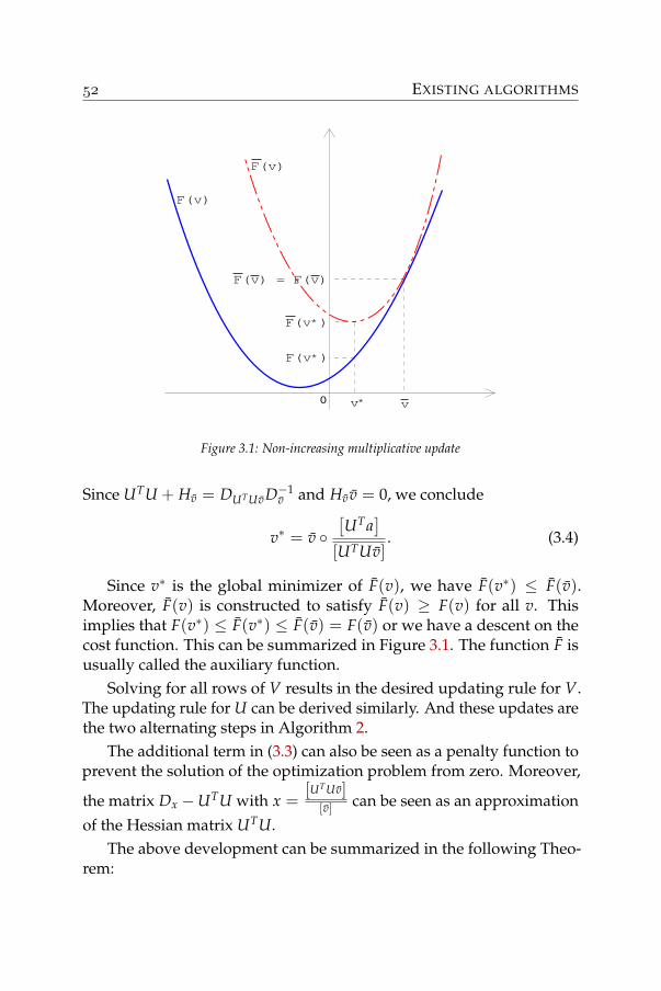
EXISTING ALGORITHMS
F(v)
v
F(v) = F(v)
F(v)
F(v )*
F(v )*
v*0
Figure 3.1: Non-increasing multiplicative update
Since UTU + Hv = DUTUvD−1v and Hvv = 0, we conclude
v∗ = v [UTa
][UTUv]
. (3.4)
Since v∗ is the global minimizer of F(v), we have F(v∗) ≤ F(v).Moreover, F(v) is constructed to satisfy F(v) ≥ F(v) for all v. Thisimplies that F(v∗) ≤ F(v∗) ≤ F(v) = F(v) or we have a descent on thecost function. This can be summarized in Figure 3.1. The function F isusually called the auxiliary function.
Solving for all rows of V results in the desired updating rule for V.The updating rule for U can be derived similarly. And these updates arethe two alternating steps in Algorithm 2.
The additional term in (3.3) can also be seen as a penalty function toprevent the solution of the optimization problem from zero. Moreover,
the matrix Dx −UTU with x =[UTUv]
[v] can be seen as an approximationof the Hessian matrix UTU.
The above development can be summarized in the following Theo-rem:
3.1 LEE AND SEUNG ALGORITHM
Algorithm 2 Multiplicative Rules (Mult)
1: Initialize U0, V0 and k = 02: repeat
3: Uk+1 = Uk [AVk][Uk(Vk)TVk]
4: Vk+1 = Vk [ATUk+1][Vk(Uk+1)TUk+1]
5: k = k + 16: until Stopping condition
Theorem 3.1. The Euclidean distance ‖A−UVT‖2F is non-increasing under
the updating rules of Algorithm 2.
Theorem 3.1 is a shortened version of the one in the original paper ofLee and Seung [80]. The original theorem has an additional part claimingthat the Euclidean distance is unchanged under the multiplicative rulesonly when it is at a stationary point. This is, in fact, not necessarily true,since if it converges, only the conditions (2.4) and (2.6) are satisfied atthe fixed point. No proof is provided to show that the conditions (2.5)can be met. There are two main obstacles in the investigation of theconvergence of these multiplicative rules.
The first one is that these multiplicative rules fail to make a sufficientdescent of the cost function. To see this, we can rewrite (3.4) as a variablemetric method [13]:
v∗ = v [UTa
][UTUv]
= v [UTa + UTUv−UTUv
][UTUv]
= v (
1 +
[UTa−UTUv
][UTUv]
)
= v− [v][UTUv]
(UTUv−UTa)
= v− Dv∇vF, (3.5)
where Dv is a positive diagonal matrix with Dii = [v]i[UTUv]i
. With this
EXISTING ALGORITHMS
update, a necessary condition for a sufficient descent is that the eigen-values of matrix Dv (i.e. Dii) must be bounded above and away fromzero [13]. But this is not true for Dv in general. Hence, the limit pointsof the algorithm may not be stationary.
The second obstacle is the possibility of zeros in U and V whenconsidering the conditions (2.5). The situation that we want to avoid is
∇Vij F < 0 while Vij = 0 (3.6)
for some (i, j) at a limit point. With the assumption that the initial U andV are positive, this problem might not happen because if, for some k:
∇Vkij
F < 0 or [Vk(Uk)TUk]ij − [AUk]ij < 0,
we have from the update:
Vk+1ij = Vk
ij[AUk]ij
[Vk(Uk)TUk]ij> Vk
ij > 0.
This is also supported by the following Lemma [85]:
Lemma 3.2. If U0 and V0 are positive and A is both row-allowable andcolumn-allowable (see Section 1.1.6), then Uk and Vk are positive.
But in practice, when using a finite precision system of number,only numbers whose magnitude is larger than the constant εM (thesmallest representable number of a number system) can be representedby nonzero numbers. Otherwise, they will be rounded to zero. Andsince we can not bound Vk
ij away from zero, it could be smaller than εM
hence represented by 0. Once Vkij = 0, the multiplicative updates will
not make it positive again. The algorithm will then be probably trappedinto a non-stationary point.
One way to avoid this is to look at every Uij = 0 (or Vij = 0), if thecorresponding element of the gradient is negative, we can set Uij = ε (orVij = ε) with ε > εM as suggested in [85] or making a gradient descentstep to the inside of the nonnegative orthant.
Remark: it is possible that [Vk(Uk)TUk]ij = 0 for some (i, j), whichresults in some zero-division exceptions. We investigate two followingpossible situations:

3.2 ALTERNATING LEAST SQUARES METHODS
• When Vkij > 0, [Vk(Uk)TUk]ij = 0 implies that
0 = ∑lt
VkitU
kltU
klj ≥ Vk
ijUkljU
klj = Vk
ij ∑l
UkljU
klj.
This occurs only when Uk:j = 0, which is due to a rank-deficient
approximation and can be fixed by generating a substitution forUk
:j.
• When Vkij = 0, we have a 0/0 situation where
∇Vij F = −[AUk]ij ≤ 0.
Then, we should not replace [Vk(Uk)TUk]ij by ε (a small positiveconstant with ε > εM) as suggested by many works, because thiswill keep Vk+1
ij = 0 which is unfavorable for the multiplicative
updates. Setting Vk+1ij = ε > εM is definitely a better choice.
The multiplicative rules are also extended to the weighted nonneg-ative matrix factorization (see Chapter 6), to the generalized Kullback-Leibler divergence (see Chapter 5) and to a broader class of cost functionnamely Bregman divergence [36]. Many other extensions can be foundin [59], [119], [83], [122], [68], etc.
3.2 Alternating least squares methods
The first algorithm proposed for solving the nonnegative matrix factor-ization was the alternating least squares method [97]. It is known that,fixing either U or V, the problem becomes a least squares problem withnonnegativity constraint.
Since the least squares problems in Algorithm 3 can be perfectlydecoupled into smaller problems corresponding to the columns or rowsof A, we can directly apply methods for the Nonnegative Least Squareproblem to each of the small problem. Methods that can be applied are[79], [44], [24], etc.
A direct application of Theorem 1.11 can show that if the subproblem(3) and (4) in Algorithm 3 are exactly and uniquely solved, every limit

EXISTING ALGORITHMS
Algorithm 3 Alternating Least Square (ALS)
1: Initialize U and V2: repeat3: Solve: minV≥0
12‖A−UVT‖2
F4: Solve: minU≥0
12‖AT −VUT‖2
F5: until Stopping condition
Algorithm 4 Inexact Alternating Least Square (IALS)
1: Initialize U and V2: repeat3: Solve for U in equation: UVTV = AV4: U = [U]+5: Solve for V in equation: VUTU = ATU6: V = [V]+7: until Stopping condition
point of Algorithm 3 is a stationary point of the nonnegative matrixfactorization problem.
But even with the faster implementation of these algorithm, theycan not match other methods in terms of running time. A modificationhas been made by replacing an exact solution of the nonnegative leastsquares problem by the projection of the solution of the unconstrainedleast squares problem into the nonnegative orthant [12] as in Algorithm4. This speeds up the algorithm by sacrifying the convergence property.Figure 3.2 is a typical example of the convergence of the AlternatingLeast Squares and the Inexact Alternating Least Squares. One can seethat while the earlier always makes a descent update, the latter doesnot. The exact method also produces better approximation errors. Butwith the same number of iterations, it spends significantly more timethan the inexact version does (3.435s vs. 0.02s). Note that the solver forthe nonnegative least squares problem in this example is the standardMatlab function lsqnonneg. For a faster solver such as [24], it is reportedthat the exact method is still far behind in terms of the running time. Inpractice, the exact Alternating Least Squares is seldomly used because itis very inefficient. And its inexact version does not, in general, converges
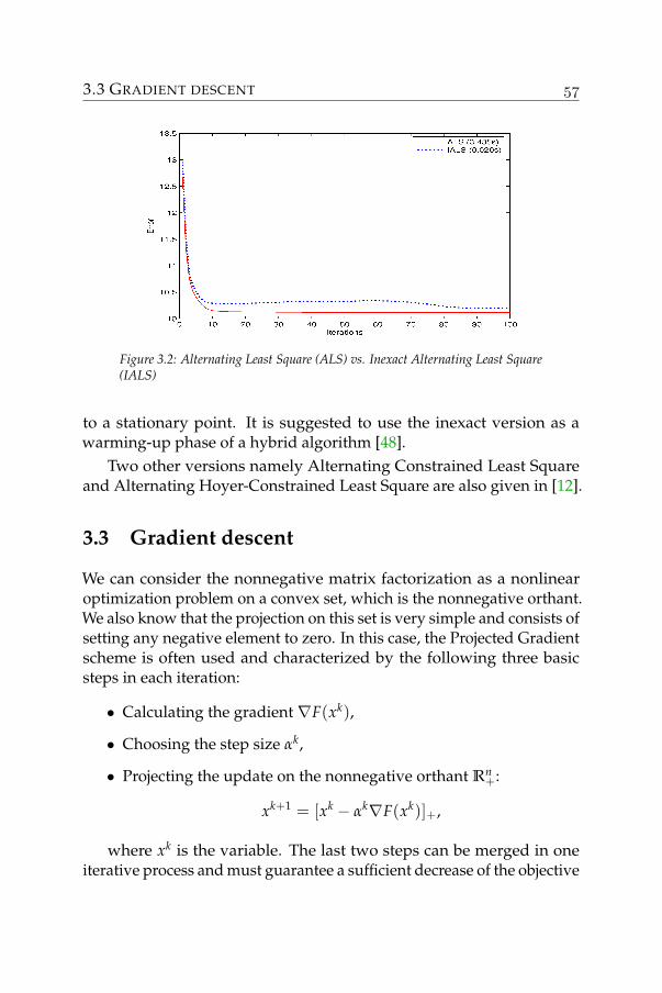
3.3 GRADIENT DESCENT
Figure 3.2: Alternating Least Square (ALS) vs. Inexact Alternating Least Square(IALS)
to a stationary point. It is suggested to use the inexact version as awarming-up phase of a hybrid algorithm [48].
Two other versions namely Alternating Constrained Least Squareand Alternating Hoyer-Constrained Least Square are also given in [12].
3.3 Gradient descent
We can consider the nonnegative matrix factorization as a nonlinearoptimization problem on a convex set, which is the nonnegative orthant.We also know that the projection on this set is very simple and consists ofsetting any negative element to zero. In this case, the Projected Gradientscheme is often used and characterized by the following three basicsteps in each iteration:
• Calculating the gradient ∇F(xk),
• Choosing the step size αk,
• Projecting the update on the nonnegative orthant Rn+:
xk+1 = [xk − αk∇F(xk)]+,
where xk is the variable. The last two steps can be merged in oneiterative process and must guarantee a sufficient decrease of the objective
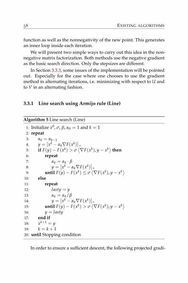
EXISTING ALGORITHMS
function as well as the nonnegativity of the new point. This generatesan inner loop inside each iteration.
We will present two simple ways to carry out this idea in the non-negative matrix factorization. Both methods use the negative gradientas the basic search direction. Only the stepsizes are different.
In Section 3.3.3, some issues of the implementation will be pointedout. Especially for the case where one chooses to use the gradientmethod in alternating iterations, i.e. minimizing with respect to U andto V in an alternating fashion.
3.3.1 Line search using Armijo rule (Line)
Algorithm 5 Line search (Line)
1: Initialize x0, σ, β, α0 = 1 and k = 12: repeat3: αk = αk−14: y = [xk − αk∇F(xk)]+5: if F(y)− F(xk) > σ
⟨∇F(xk), y− xk⟩ then
6: repeat7: αk = αk · β8: y = [xk − αk∇F(xk)]+9: until F(y)− F(xk) ≤ σ
⟨∇F(xk), y− xk⟩
10: else11: repeat12: lasty = y13: αk = αk/β14: y = [xk − αk∇F(xk)]+15: until F(y)− F(xk) > σ
⟨∇F(xk), y− xk⟩
16: y = lasty17: end if18: xk+1 = y19: k = k + 120: until Stopping condition
In order to ensure a sufficient descent, the following projected gradi-
3.3 GRADIENT DESCENT
ent scheme with Armijo criterion [86] can be applied to minimize
x∗ = argminx
F(x).
Algorithm 5 needs two parameters σ and β that may affect its con-vergence. It requires only the gradient information, and is applied in[86] for two different strategies : for the whole space (U, V) (AlgorithmFLine) and for U and V separately in an alternating fashion (AlgorithmCLine). With a good choice of parameters (σ = 0.01 and β = 0.1) and agood strategy of alternating between variables, it was reported in [86]to be the faster than the multiplicative rules.
3.3.2 Gradient Projection using first order approximation
In order to find the solution to the problem:
x∗ = argminx
F(x)
we can also approximate at each iteration the function F(X) using:
F(x) = F(xk) +⟨∇xF(xk), x− xk
⟩+
L2‖xk − x‖2
2,
where L is a Lipschitz constant, the smallest value of L satisfying F(x) ≤F(x), ∀x.
Because of this inequality, the solution of the following problem
xk+1 = argminx≥0
F(x)
also is a point of descent for the function F(x) since
F(xk+1) ≤ F(xk+1) ≤ F(xk) = F(xk).
Since the constant L is not known a priori, an inner loop is needed.Algorithm 6 presents an iterative way to carry out this scheme. As inthe previous algorithm this also requires only the gradient informationand can therefore can be applied to two different strategies: to thewhole space (U, V) (Algorithm FFO) and to U and V separately in analternating fashion (Algorithm CFO).
A main difference with the previous algorithm is its stopping crite-rion for the inner loop. This algorithm requires also a parameter β forwhich the practical choice is 2.
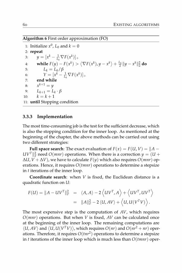
EXISTING ALGORITHMS
Algorithm 6 First order approximation (FO)
1: Initialize x0, L0 and k = 02: repeat3: y = [xk − 1
Lk∇F(xk)]+
4: while F(y)− F(xk) >⟨∇F(xk), y− xk⟩+ Lk
2 ‖y− xk‖22 do
5: Lk = Lk/β6: Y = [xk − 1
Lk∇F(xk)]+
7: end while8: xk+1 = y9: Lk+1 = Lk · β
10: k = k + 111: until Stopping condition
3.3.3 Implementation
The most time-consuming job is the test for the sufficient decrease, whichis also the stopping condition for the inner loop. As mentioned at thebeginning of the chapter, the above methods can be carried out usingtwo different strategies:
Full space search: The exact evaluation of F(x) = F(U, V) = ‖A−UVT‖2
F need O(mnr) operations. When there is a correction y = (U +∆U, V + ∆V), we have to calculate F(y) which also requires O(mnr) op-erations. Hence, it requires O(tmnr) operations to determine a stepsizein t iterations of the inner loop.
Coordinate search: when V is fixed, the Euclidean distance is aquadratic function on U:
F(U) = ‖A−UVT‖2F = 〈A, A〉 − 2
⟨UVT, A
⟩+⟨
UVT, UVT⟩
= ‖A‖2F − 2 〈U, AV〉+
⟨U, U(VTV)
⟩.
The most expensive step is the computation of AV, which requiresO(mnr) operations. But when V is fixed, AV can be calculated onceat the beginning of the inner loop. The remaining computations are〈U, AV〉 and
⟨U, U(VTV)
⟩, which requires O(nr) and O(nr2 + nr) oper-
ations. Therefore, it requires O(tnr2) operations to determine a stepsizein t iterations of the inner loop which is much less than O(tmnr) oper-
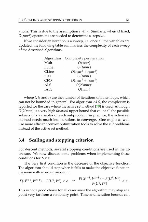
3.4 SCALING AND STOPPING CRITERION
ations. This is due to the assumption r n. Similarly, when U fixed,O(tmr2) operations are needed to determine a stepsize.
If we consider an iteration is a sweep, i.e. once all the variables areupdated, the following table summarizes the complexity of each sweepof the described algorithms:
Algorithm Complexity per iterationMult O(mnr)FLine O(tmnr)CLine O(t1nr2 + t2mr2)FFO O(tmnr)CFO O(t1nr2 + t2mr2)ALS O(2rmnr)∗
IALS O(mnr)
where t, t1 and t2 are the number of iterations of inner loops, whichcan not be bounded in general. For algorithm ALS, the complexity isreported for the case where the active set method [79] is used. AlthoughO(2rmnr) is a very high theorical upper bound that count all the possiblesubsets of r variables of each subproblem, in practice, the active setmethod needs much less iterations to converge. One might as welluse more efficient convex optimization tools to solve the subproblemsinstead of the active set method.
3.4 Scaling and stopping criterion
For descent methods, several stopping conditions are used in the lit-erature. We now discuss some problems when implementing theseconditions for NMF.
The very first condition is the decrease of the objective function.The algorithm should stop when it fails to make the objective functiondecrease with a certain amount :
F(Uk+1, Vk+1)− F(Uk, Vk) < ε orF(Uk+1, Vk+1)− F(Uk, Vk)
F(Uk, Vk)< ε.
This is not a good choice for all cases since the algorithm may stop at apoint very far from a stationary point. Time and iteration bounds can
EXISTING ALGORITHMS
also be imposed for very slowly converging algorithms. But here againthis may not be good for the optimality conditions. A better choice isprobably the norm of the projected gradient as suggested in [86]. Forthe NMF problem it is defined as follows :
[∇PX]ij =
[∇X]ij if Xij > 0min(0, [∇X]ij) if Xij = 0
where X stands for U or V. The proposed condition then becomes∥∥∥∥( ∇PUk
∇PVk
)∥∥∥∥F≤ ε
∥∥∥∥( ∇U1
∇V1
)∥∥∥∥F
. (3.7)
We should also take into account the scaling invariance between U andV. Putting U = γU and V = 1
γ V does not change the approximationUVT but the above projected gradient norm is affected:∥∥∥∥( ∇P
U∇P
V
)∥∥∥∥2
F= ‖∇P
U‖2F + ‖∇P
V‖2F =
1γ2 ‖∇
PU‖2
F + γ2‖∇PV‖2
F (3.8)
6=∥∥∥∥( ∇P
U∇P
V
)∥∥∥∥2
F.
Two approximate factorizations UVT = UVT resulting in the sameapproximation should be considered equivalent in terms of precision.One could choose γ2 := ‖∇P
U‖F/‖∇PV‖F, which minimizes (3.8) and
forces ‖∇PU‖F = ‖∇P
V‖F, but this may not be a good choice when onlyone of the gradients ‖∇P
U‖F and ‖∇PV‖F is nearly zero.
In fact, the gradient(∇U∇V
)is scale dependent in the NMF problem
and any stopping criterion that uses gradient information is affected bythis scaling. To limit that effect, we suggest the following scaling aftereach iteration:
Uk ← UkDk Vk ← VkD−1k
where Dk is a positive diagonal matrix:
[Dk]ii =
√‖V:i‖2
‖U:i‖2.
3.5 INITIALIZATIONS
This ensures that ‖U:i‖2F = ‖V:i‖2
F and hopefully reduces also the differ-ence between ‖∇P
U‖2F and ‖∇P
V‖2F. Moreover, it may help to avoid some
numerically unstable situations.The same scaling should be applied to the initial point as well
(U1, V1) when using (3.7) as the stopping condition.
3.5 Initializations
We know that the nonnegative matrix factorization problem is not con-vex, and hence expect it to have local minima. Moreover, starting from apoint too far from the stationary points costs any iterative method manyiterations before getting close to one such stationary point. A good initialapproximation could not only shift the interest to good local minimabut would also help to reduce the number of iterations. Several tech-niques are proposed in the literature. Among them, an application ofthe Spherical K-Means algorithm [127] to generate an initial point showsa nice improvement but is too expensive. This is not surprising sinceK-Means is in fact an instance of NMF factorization, as we mentionedin the introduction. Other interesting methods proposed in [2] providesome ideas but have a small improvement over the random initialization.The best reported method is the SVD-centroid which requires a partialSVD decomposition of the original matrix, which is not always availableand needs to be computed. Recently proposed method [20] takes therank-r SVD decomposition UΣVT of the target matrix A, removes all thenegative values of U and V and creates a simple rank-2r nonnegativefactorization as an initialization. Although a loose upper bound of theerror can be derived, this method again needs a SVD decomposition.These mentioned methods is reported to behave well for some specificdatasets and algorithms, but they may not be as good when applied toother cases. A deeper investigation will be necessary.
Since nothing is known about the distribution of the minima, webelieve that a random initialization maybe a good starting point. In fact,in most existing applications, a random initialization is used because ofits simplicity. We have to point out that, using directly a random initial-ization is very naive, and a preprocessing step can improve significantlythe quality of the initial point. For example, the following step can be

EXISTING ALGORITHMS
applied to algorithms which are sensitive to scalings (multiplicativeupdates and gradient methods):
α :=⟨
A, U0VT0⟩⟨
U0VT0 , U0VT
0
⟩ , U0 = U0√
α, V0 = V0√
α,
where the scaling factor α is in fact the optimal solution of the problem:
minα‖A− αU0VT
0 ‖2F.
4
RANK-ONE RESIDUE ITERATION
In the previous chapter, we have seen that it is very appealing to decou-ple the problem into convex subproblems. But this may “converge” tosolutions that are far from the global minimizers of the problem.
This chapter is an extension of the internal report [62], where weproposed to decouple the problem based on rank-one approximations tocreate a new algorithm. A convergence analysis, numerical experimentsand some extensions were also presented for this algorithm. Duringthe completion of the revised version of this report, we were informedthat two other independent reports [31] and [49] had also proposed thisalgorithm.
This algorithm has several advantages : it allows us to formulatea very simple basic subproblem, which can be solved in closed form,seems to have useful convergence results and can be extended to moregeneral types of factorizations such as for nonnegative tensors. More-over, the experiments in Section 4.7 suggest that this new method out-performs the other ones in most cases.
Here, we present an introduction and an analysis of this algorithm,compare it with existing algorithms and test new extensions.
4.1 Motivation
NMF problem is, in fact, a least square problem with nonnegativity con-straints. The classical nonnegative least square problem [79] is definedas below:
RANK-ONE RESIDUE ITERATION
Problem 4.1 (NNLS).minx≥0‖Ax− b‖2
F.
As we can see NMF problem can be decoupled into several problems4.1. Therefore it is quite natural to apply any method for the aboveproblem to solve the NMF problem. The standard one is the activeset method proposed by Lawson and Hanson [79]. But even with theimproved version by Bro and Jong [24], using this for NMF problem stillappears very slow.
One of the main reasons lies in the reusability of the computations.The decoupling helps to break the NMF problem into smaller problemsbut for many methods, solving a decoupled NNLS problem may nothelp for solving other NNLS problems. We are talking about solving anumber of separate nonnegative least square problems
minx≥0‖A:,i −Ux‖2
F, i = 1, 2, ..., n.
The active set method actually consists in solving a sequence of normalequations where a number of pseudo-inverse matrices need to be com-puted. These computations could be reused to speed up solving formultiple columns of A [74][24].
These methods start with all the columns of U to solve the nor-mal equation UTUx = UT A:,i where one needs to compute U+ =(UTU)−1U. At each iteration, several columns of U are removed creat-ing smaller matrices U1, U2, . . . Then, Ui+ = (UiTUi)−1Ui are computed.Clearly, keeping and reusing all (Ui)+ matrices is impossible for largeproblem, since the number of those matrices might be 2r, total numberof possible subsets from r columns of U.
In [44], a different strategy is deployed to create an iterative method.At each iteration, only one element xi is updated. The elementary prob-lem to be solved is:
Problem 4.2.min
xi∈R+‖xiU:,i − ri‖2
F,
where ri = A:,i −∑j 6=i xjU(:, j) is the residue vector.
4.2 COLUMN PARTITION OF VARIABLES
The optimal solution to this problem is trivially given by
x∗i = max
( ⟨ri, U:,i
⟩〈U:,i, U:,i〉
, 0
).
In fact, this is an instance of Problem 4.1 where U has only one column.And U+
:,i = U:,i〈U:,i ,U:,i〉 can be reused when there are multiple columns of A.
We will use this idea to create an iterative method for the standardNMF problem and derive other NMF problems. An iterative methodfor Nonnegative Tensor Factorization (NTF) will also be derived.
4.2 Column partition of variables
Let the ui’s and vi’s be respectively the columns of U and V. Then theNMF problem can be rewritten as follows :
Problem 4.3 (Nonnegative Matrix Factorization). Given a m× n non-negative matrix A, solve
minui≥0 vi≥0
12‖A−
r
∑i=1
uivTi ‖2
F.
Let us fix all the variables, except for a single vector vt and considerthe following least squares problem:
minv≥0
12‖Rt − utvT‖2
F, (4.1)
where Rt = A−∑i 6=t uivTi . We have:
‖Rt − utvT‖2F = trace
[(Rt − utvT)T(Rt − utvT)
](4.2)
= ‖Rt‖2F − 2vTRT
t ut + ‖ut‖22‖v‖2
2. (4.3)
From this formulation, one now derives the following lemma.
Lemma 4.4. If [RTt ut]+ 6= 0, then v∗ := [RT
t ut]+‖ut‖2
2is the unique global mini-
mizer of (4.1) and the function value equals ‖Rt‖2F −
‖[RTt ut]+‖2
2‖ut‖2
2.
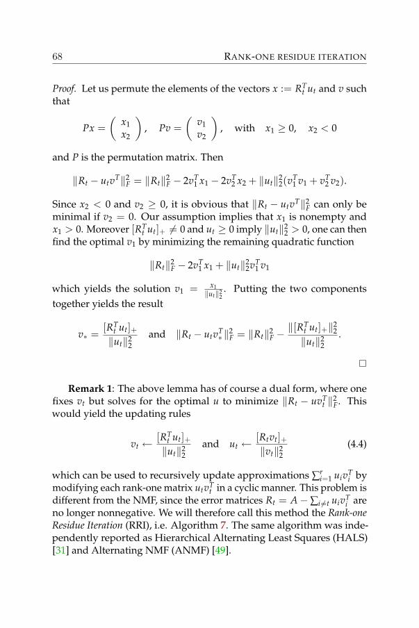
RANK-ONE RESIDUE ITERATION
Proof. Let us permute the elements of the vectors x := RTt ut and v such
that
Px =(
x1x2
), Pv =
(v1v2
), with x1 ≥ 0, x2 < 0
and P is the permutation matrix. Then
‖Rt − utvT‖2F = ‖Rt‖2
F − 2vT1 x1 − 2vT
2 x2 + ‖ut‖22(vT
1 v1 + vT2 v2).
Since x2 < 0 and v2 ≥ 0, it is obvious that ‖Rt − utvT‖2F can only be
minimal if v2 = 0. Our assumption implies that x1 is nonempty andx1 > 0. Moreover [RT
t ut]+ 6= 0 and ut ≥ 0 imply ‖ut‖22 > 0, one can then
find the optimal v1 by minimizing the remaining quadratic function
‖Rt‖2F − 2vT
1 x1 + ‖ut‖22vT
1 v1
which yields the solution v1 = x1‖ut‖2
2. Putting the two components
together yields the result
v∗ =[RT
t ut]+‖ut‖2
2and ‖Rt − utvT
∗ ‖2F = ‖Rt‖2
F −‖[RT
t ut]+‖22
‖ut‖22
.
Remark 1: The above lemma has of course a dual form, where onefixes vt but solves for the optimal u to minimize ‖Rt − uvT
t ‖2F. This
would yield the updating rules
vt ←[RT
t ut]+‖ut‖2
2and ut ←
[Rtvt]+‖vt‖2
2(4.4)
which can be used to recursively update approximations ∑ri=1 uivT
i bymodifying each rank-one matrix utvT
t in a cyclic manner. This problem isdifferent from the NMF, since the error matrices Rt = A−∑i 6=t uivT
i areno longer nonnegative. We will therefore call this method the Rank-oneResidue Iteration (RRI), i.e. Algorithm 7. The same algorithm was inde-pendently reported as Hierarchical Alternating Least Squares (HALS)[31] and Alternating NMF (ANMF) [49].
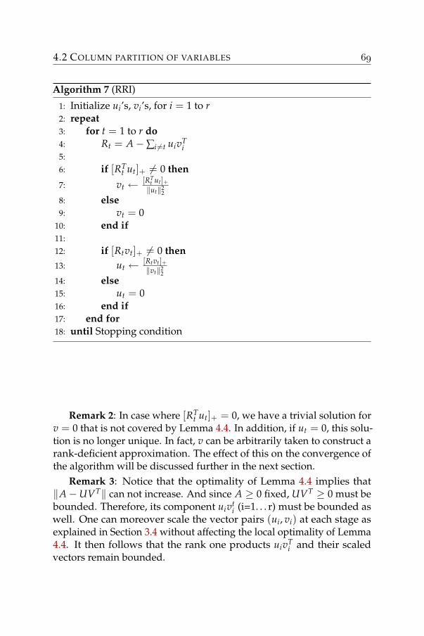
4.2 COLUMN PARTITION OF VARIABLES
Algorithm 7 (RRI)
1: Initialize ui’s, vi’s, for i = 1 to r2: repeat3: for t = 1 to r do4: Rt = A−∑i 6=t uivT
i5:6: if [RT
t ut]+ 6= 0 then7: vt ← [RT
t ut]+‖ut‖2
28: else9: vt = 0
10: end if11:12: if [Rtvt]+ 6= 0 then13: ut ← [Rtvt]+
‖vt‖22
14: else15: ut = 016: end if17: end for18: until Stopping condition
Remark 2: In case where [RTt ut]+ = 0, we have a trivial solution for
v = 0 that is not covered by Lemma 4.4. In addition, if ut = 0, this solu-tion is no longer unique. In fact, v can be arbitrarily taken to construct arank-deficient approximation. The effect of this on the convergence ofthe algorithm will be discussed further in the next section.
Remark 3: Notice that the optimality of Lemma 4.4 implies that‖A−UVT‖ can not increase. And since A ≥ 0 fixed, UVT ≥ 0 must bebounded. Therefore, its component uivt
i (i=1. . . r) must be bounded aswell. One can moreover scale the vector pairs (ui, vi) at each stage asexplained in Section 3.4 without affecting the local optimality of Lemma4.4. It then follows that the rank one products uivT
i and their scaledvectors remain bounded.
RANK-ONE RESIDUE ITERATION
4.3 Convergence
In the previous section, we have established the partial updates for eachof the variable ui or vi. And for a NMF problem where the reduced rankis r, we have in total 2r vector variables (the ui’s and vi’s). The describedalgorithm can be also considered as a projected gradient method sincethe update (4.4) can be rewritten as:
ut ←[Rtvt]+‖vt‖2
2=
[(A−∑i 6=t uivTi )vt]+
‖vt‖22
=[(A−∑i uivT
i + utvTt )vt]+
‖vt‖22
=[(A−∑i uivT
i )vt + utvTt vt]+
‖vt‖22
=[
ut −1‖vt‖2
2∇ut
]+
.
Similarly, the update for vi can be rewritten as
vt ←[
vt −1‖ut‖2
2∇vt
]+
.
Therefore, the new method follows the projected gradient schemedescribed in the previous section. But it produces the optimal solutionin closed form. For each update of a column vt (or ut), the proposedalgorithm requires just a matrix-vector multiplication RT
t ut (or Rtvt),wherein the residue matrix Rt = A − ∑i 6=t uivT
i does not have to becalculated explicitly. Indeed, by calculating RT
t ut (or Rtvt) from ATut(or Avt) and ∑i 6=t vi(uT
i ut) (or ∑i 6=t ui(vTi vt)), the complexity is reduced
from O(mnr + mn) to only O (mn + (m + n)(r− 1)) which is majoredby O(mn). This implies that the complexity of each sweep throughthe 2r variables u′ts and v′ts requires only O(mnr) operations, which isequivalent to a sweep of the multiplicative rules and to an inner loopof any gradient methods. This is very low since the evaluation of thewhole gradient requires already the same complexity.
Because at each step of the 2r basic steps of Algorithm 7, we computean optimal rank-one nonnegative correction to the corresponding errormatrix Rt the Frobenius norm of the error can not increase. This is areassuring property but it does not imply convergence of the algorithm.
Each vector ut or vt lies in a convex set Ut ⊂ Rm+ or Vt ⊂ Rn
+.Moreover, because of the possibility to include scaling we can set an
4.3 CONVERGENCE
upper bound for ‖U‖ and ‖V‖, in such a way that all the Ut and Vtsets can be considered as closed convex. Then, we can use the followingTheorem 4.5, to prove a stronger convergence result for Algorithm 7.
Theorem 4.5. Every limit point generated by Algorithm 7 is a stationarypoint.
Proof. We notice that, if ut = 0 and vt = 0 at some stages of Algorithm 7,they will remain zero and no longer take part in all subsequent iterations.We can divide the execution of Algorithm 7 into two phases.
During the first phase, some of the pairs (ut, vt) become zero. Be-cause there are only a finite number (2r) of such vectors, the number ofiterations in this phase is also finite. At the end of this phase, we canrearrange and partition the matrices U and V such that
U = (U+ 0) and V = (V+ 0),
where U+ and V+ do not have any zero column. We temporarily removezero columns out of the approximation.
During the second phase, no column of U+ and V+ becomes zero,which guarantees the updates for the columns of U+ and V+ are uniqueand optimal. Moreover, 1
2‖A − ∑ri=1 uivT
i ‖2F is continuously differen-
tiable over the set U1 × . . .×Ur ×V1 × . . .×Vr, and the Ui’s and Vi’sare closed convex. A direct application of Theorem 1.11 proves thatevery stationary point (U∗+, V∗+) is a stationary point. It is then easy toprove that if there are zero columns removed at the end of the first phase,adding them back yields another stationary point: U∗ = (U∗+ 0) andV∗ = (V∗+ 0) of the required dimension. However, in this case, the rankof the approximation will then be lower than the requested dimensionr.
In Algorithm 7, variables are updated in this order: u1, v1, u2, v2,. . .. We can alternate the variables in a different order as well, for ex-ample u1, u2, . . ., ur v1, v2, . . ., vr, . . .. Whenever this is carried out in acyclic fashion, the Theorem 4.5 still holds and this does not increase thecomplexity of each iteration of the algorithm.
As pointed above, stationary points given by Algorithm 7 maycontain useless zero components. To improve this, one could replace
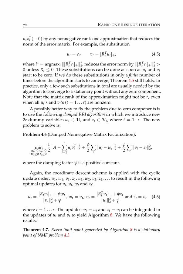
RANK-ONE RESIDUE ITERATION
utvTt (≡ 0) by any nonnegative rank-one approximation that reduces the
norm of the error matrix. For example, the substitution
ut = ei∗ vt = [RTt ut]+, (4.5)
where i∗ = argmaxi ‖[RTt ei]+‖2
2, reduces the error norm by ‖[RTt ei]+‖2
2 >0 unless Rt ≤ 0. These substitutions can be done as soon as ut and vtstart to be zero. If we do these substitutions in only a finite number oftimes before the algorithm starts to converge, Theorem 4.5 still holds. Inpractice, only a few such substitutions in total are usually needed by thealgorithm to converge to a stationary point without any zero component.Note that the matrix rank of the approximation might not be r, evenwhen all ut’s and vt’s (t = 1 . . . r) are nonzero.
A possibly better way to fix the problem due to zero components isto use the following damped RRI algorithm in which we introduce new2r dummy variables wi ∈ Ui and zi ∈ Vi, where i = 1...r. The newproblem to solve is:
Problem 4.6 (Damped Nonnegative Matrix Factorization).
minui≥0 vi≥0wi≥0 zi≥0
12‖A−
r
∑i=1
uivTi ‖2
F +ψ
2 ∑i‖ui − wi‖2
2 +ψ
2 ∑i‖vi − zi‖2
2,
where the damping factor ψ is a positive constant.
Again, the coordinate descent scheme is applied with the cyclicupdate order: u1, w1, v1, z1, u2, w2, v2, z2, . . . to result in the followingoptimal updates for ut, vt, wt and zt:
ut =[Rtvt]+ + ψwt
‖vt‖22 + ψ
, wt = ut, vt =[RT
t ut]+ + ψzt
‖ut‖22 + ψ
and zt = vt (4.6)
where t = 1 . . . r. The updates wt = ut and zt = vt can be integrated inthe updates of ut and vt to yield Algorithm 8. We have the followingresults:
Theorem 4.7. Every limit point generated by Algorithm 8 is a stationarypoint of NMF problem 4.3.
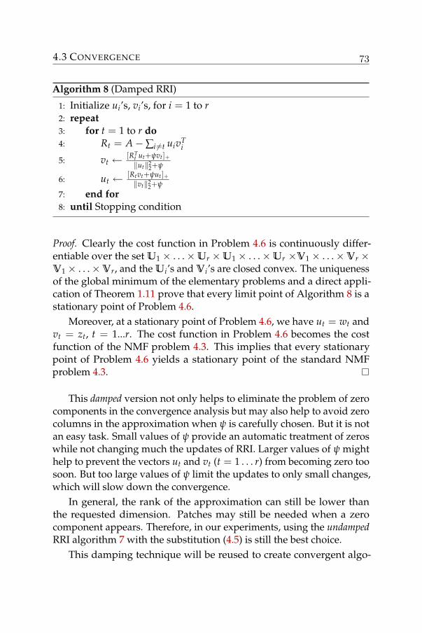
4.3 CONVERGENCE
Algorithm 8 (Damped RRI)
1: Initialize ui’s, vi’s, for i = 1 to r2: repeat3: for t = 1 to r do4: Rt = A−∑i 6=t uivT
i
5: vt ← [RTt ut+ψvt]+‖ut‖2
2+ψ
6: ut ← [Rtvt+ψut]+‖vt‖2
2+ψ
7: end for8: until Stopping condition
Proof. Clearly the cost function in Problem 4.6 is continuously differ-entiable over the set U1 × . . .×Ur ×U1 × . . .×Ur ×V1 × . . .×Vr ×V1 × . . .×Vr, and the Ui’s and Vi’s are closed convex. The uniquenessof the global minimum of the elementary problems and a direct appli-cation of Theorem 1.11 prove that every limit point of Algorithm 8 is astationary point of Problem 4.6.
Moreover, at a stationary point of Problem 4.6, we have ut = wt andvt = zt, t = 1...r. The cost function in Problem 4.6 becomes the costfunction of the NMF problem 4.3. This implies that every stationarypoint of Problem 4.6 yields a stationary point of the standard NMFproblem 4.3.
This damped version not only helps to eliminate the problem of zerocomponents in the convergence analysis but may also help to avoid zerocolumns in the approximation when ψ is carefully chosen. But it is notan easy task. Small values of ψ provide an automatic treatment of zeroswhile not changing much the updates of RRI. Larger values of ψ mighthelp to prevent the vectors ut and vt (t = 1 . . . r) from becoming zero toosoon. But too large values of ψ limit the updates to only small changes,which will slow down the convergence.
In general, the rank of the approximation can still be lower thanthe requested dimension. Patches may still be needed when a zerocomponent appears. Therefore, in our experiments, using the undampedRRI algorithm 7 with the substitution (4.5) is still the best choice.
This damping technique will be reused to create convergent algo-
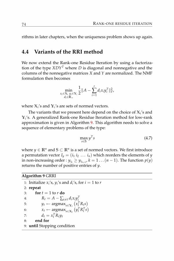
RANK-ONE RESIDUE ITERATION
rithms in later chapters, when the uniqueness problem shows up again.
4.4 Variants of the RRI method
We now extend the Rank-one Residue Iteration by using a factoriza-tion of the type XDYT where D is diagonal and nonnegative and thecolumns of the nonnegative matrices X and Y are normalized. The NMFformulation then becomes
minxi∈Xi yi∈Yi
di∈R+
12‖A−
r
∑i=1
dixiyTi ‖2
F,
where Xi’s and Yi’s are sets of normed vectors.The variants that we present here depend on the choice of Xi’s and
Yi’s. A generalized Rank-one Residue Iteration method for low-rankapproximation is given in Algorithm 9. This algorithm needs to solve asequence of elementary problems of the type:
maxs∈S
yTs (4.7)
where y ∈ Rn and S ⊂ Rn is a set of normed vectors. We first introducea permutation vector Iy = (i1 i2 . . . in) which reorders the elements of yin non-increasing order : yik ≥ yik+1 , k = 1 . . . (n− 1). The function p(y)returns the number of positive entries of y.
Algorithm 9 GRRI
1: Initialize xi’s, yi’s and di’s, for i = 1 to r2: repeat3: for t = 1 to r do4: Rt = A−∑i 6=t dixiyT
i5: yt ← argmaxs∈Yt
(xT
t Rts)
6: xt ← argmaxs∈Xt
(yT
t RTt s)
7: dt = xTt Rtyt
8: end for9: until Stopping condition

4.4 VARIANTS OF THE RRI METHOD
Let us first point out that for the set of normed nonnegative vectorsthe solution of problem (4.7) is given by s∗ = y+
‖y+‖2. It then follows that
Algorithm 9 is essentially the same as Algorithm 7 since the solutions viand ui of each step of Algorithm 9, given by (4.4), correspond exactly tothose of problem (4.7) via the relations yi = ui/‖ui‖2, yi = vi/‖vi‖2 anddi = ‖ui‖2‖vi‖2.
Below we list the sets for which the solution s∗ of (4.7) can be easilycomputed.
• Set of normed nonnegative vectors: s = y+‖y+‖2
.
• Set of normed bounded nonnegative vectors s: where 0 ≤ li ≤ si ≤pi. The optimal solution of (4.7) is given by:
s = max(
l, min(
p,y+
‖y+‖2
)).
• Set of normed binary vectors s: where s = b‖b‖ and b ∈ 0, 1n. The
optimal solution of (4.7) is given by:
[s∗]it =
1√k∗
if t ≤ k∗
0 otherwisewhere k∗ = argmax
k
∑kt=1 yit√
k.
• Set of normed sparse nonnegative vectors: all normed nonnegativevectors having at most K nonzero entries. The optimal solution for(4.7) is given by norming the following vector p∗
[p∗]it =
yit if t ≤ min(p(y), K)0 otherwise
• Set of normed fixed-sparsity nonnegative vectors: all nonnegative vec-tors s a fixed sparsity, where
sparsity(s) =√
n− ‖s‖1/‖s‖2√n− 1
.
The optimal solution for (4.7) is given by using the projectionscheme in [68].
RANK-ONE RESIDUE ITERATION
One can also imagine other variants, for instance by combining theabove ones. Depending on how data need to be approximated, one cancreate new algorithms provided it is relatively simple to solve problem(4.7). There have been some particular ideas in the literatures such asNMF with sparseness constraint [68], Semidiscrete Matrix Decompo-sition [76] and Semi-Nonnegative Matrix Factorization [38] for whichvariants of the above scheme can offer an alternative choice of algorithm.
Remark: Only the first two sets are the normed version of a closedconvex set, as required for the convergence by Theorem 4.5. Thereforethe algorithms might not converge to a stationary point with the othersets. However, the algorithm always guarantees a non-increasing up-date even in those cases and can therefore be expected to return a goodapproximation.
4.5 Regularizations
The regularizations are common methods to cope with the ill-posednessof inverse problems. Having known some additional information aboutthe solution, one may want to imposed a priori some constraints toalgorithms, such as: smoothness, sparsity, discreteness, etc. To addsuch regularizations in to the RRI algorithms, it is possible to modifythe NMF cost function by adding some regularizing terms. We willlist here the update for ui’s and vi’s when some simple regularizationsare added to the original cost function. The proof of these updates arestraight-forward and hence omitted.
• One-Norm ‖.‖1 regularization: the one-norm of the vector variablecan be added as a heuristic for finding a sparse solution. This isan alternative to the fixed-sparsity variant presented above. Theregularized cost function with respect to the variable vt will be
12‖Rt − utvT‖2
F + β‖v‖1, β > 0
where the optimal update is given by
v∗t =[RT
t ut − β1n×1]+‖ut‖2
2.
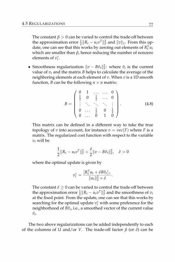
4.5 REGULARIZATIONS
The constant β > 0 can be varied to control the trade-off betweenthe approximation error 1
2‖Rt − utvT‖2F and ‖v‖1. From this up-
date, one can see that this works by zeroing out elements of RTt ut
which are smaller than β, hence reducing the number of nonzeroelements of v∗t .
• Smoothness regularization ‖v − Bvt‖2F: where vt is the current
value of vt and the matrix B helps to calculate the average of theneighboring elements at each element of v. When v is a 1D smoothfunction, B can be the following n× n matrix:
B =
0 1 . . . . . . 012 0 1
2 . . . 0...
. . . . . . . . ....
0 . . . 12 0 1
20 . . . 0 1 0
. (4.8)
This matrix can be defined in a different way to take the truetopology of v into account, for instance v = vec(F) where F is amatrix. The regularized cost function with respect to the variablevt will be
12‖Rt − utvT‖2
F +δ
2‖v− Bvt‖2
F, δ > 0
where the optimal update is given by
v∗t =[RT
t ut + δBvt]+‖ut‖2
2 + δ.
The constant δ ≥ 0 can be varied to control the trade-off betweenthe approximation error 1
2‖Rt − utvT‖2F and the smoothness of vt
at the fixed point. From the update, one can see that this works bysearching for the optimal update v∗t with some preference for theneighborhood of Bvi, i.e., a smoothed vector of the current valuevt.
The two above regularizations can be added independently to eachof the columns of U and/or V. The trade-off factor β (or δ) can be
RANK-ONE RESIDUE ITERATION
different for each column. A combination of different regularizations ona column (for instance vt) can also be used to solve the multi-criterionproblem
12‖Rt − utvT‖2
F +γ
2‖v‖2
2 +δ
2‖v− Bvt‖2
F, β, γ, δ > 0
where the optimal update is given by
v∗t =[RT
t ut − β1n×1 + δBvt]+‖ut‖2
2 + δ.
The one-norm regularizations as well as the two-norm regularizationcan be found in [2] and [12]. A major difference with that method is thatthe norm constraints is added to the rows rather than on the columnsof V or U as done here. However, for the two versions of the one-normregularization, the effects are somehow similar. While the two-normregularization on the columns of U and V are simply scaling effects,which yield nothing in the RRI algorithm. We therefore only test thesmoothness regularization at the end of the chapter with some numericalgenerated data.
In Chapter 7, a regularization will be added as an attempt to find asymmetric nonnegative approximation.
4.6 Algorithms for NMF extensions
In Section 2.4, two important extensions are introduced. In this section,we will derive the above algorithms to those extensions.
4.6.1 Multilayer nonnegative matrix factorization
We restate the multilayer nonnegative matrix factorization
minXi≥0
12‖A− X1X1 . . . XN‖2
F, (4.9)
where A is the nonnegative data matrix and V and Xi’s are nonnegativematrix of compatible sizes.
4.6 ALGORITHMS FOR NMF EXTENSIONS
We derive here a coordinate descent algorithm based on the aboverank-one iteration. We create some intermediate matrices:
Uk = X1X2 . . . Xk and Vk = XTNXT
N−1 . . . XTk , with k = 1, 2, . . . , N,
and U0 = Im and VN+1 = In.With those matrices, restricting to only one factor Xk, Problem 4.9
can be related as follows:
minXk≥0
12‖A−Uk−1XkVT
k+1‖2F, with k = 1, . . . , N.
The updates for X1 and XN are easy. Since the problem becomesexactly that of the two-factor factorization, i.e.
minX1≥0
12‖A− X1VT
2 ‖2F and min
XN≥0
12‖A−UN−1XN‖2
F.
To derive updates for the elements of Xk, k = 2, . . . , (N − 1), wetransform the product Uk−1XkVT
k+1 into a vector using the operator vec()
vec(Uk−1XkVTk+1) = (Vk+1 ⊗Uk−1)vec(Xk).
Then the optimal Xk can be found by the following nonnegative leastsquare
minvec(X)≥0
12‖vec(A)− (Vk+1 ⊗Uk−1)vec(X)‖2
F
to which algorithms such as [79] and [24] can be applied. One can alsoderive updates for each element of Xk, as done in [44], which gives thefollowing closed form update
[Xk]ij = max
(0, [Xk]ij +
[Uk−1]T:i E[Vk+1]:j
‖[Uk−1]:i‖22 ‖[Vk+1]:j‖2
2
),
where E = A−Uk−1XkVTk+1.
The approach proposed here is different from that in [29, 32] where anew layer is created by factorizing the last achieved layer using a NMFalgorithm. First, a NMF factorization is created: A ≈ X1A1. Then thenewly created matrix A1 is approximated by X2A2. This is repeated tocreate X3, X4, . . . until the desired number of layers is reached. Clearly,the approximation error will be higher than our proposed method, sincethe cost function is minimized by taking into account all the layers.
RANK-ONE RESIDUE ITERATION
4.6.2 Nonnegative tensor factorization
If we refer to the problem of finding the nearest nonnegative vector toa given vector a as the nonnegative approximation in one dimension,the NMF is its generalization in two dimensions and naturally, it can beextended to even higher-order tensor approximation problems. Algo-rithms described in the previous section use the closed form solutionof the one dimensional problem to solve the two-dimensional problem.We now generalize this to higher orders. Since in one dimension suchan approximation is easy to construct, we continue to use this approachto build the solutions for higher order problems.
For a low-rank tensor, there are two popular kinds of factored tensors,namely those of Tucker and Kruskal [5]. We only give an algorithm forfinding approximations of Kruskal type. It is easy to extend this totensors of Tucker type, but this is omitted here.
Given a d dimensional tensor T, we will derive an algorithm forapproximating a nonnegative tensor by a rank-r nonnegative Kruskaltensor S ∈ R
n1×n2×...×nd+ represented as a sum of r rank-one tensors:
S =r
∑i=1
σiu1i ? u2i ? . . . ? udi
where σi ∈ R+ is a scaling factor, uti ∈ Rnt+ is a normed vector (i.e.
‖uti‖2 = 1) and a ? b stands for the outer product between two vectorsor tensors a and b.
The following update rules are the generalization of the matrix caseto the higher order tensor:
y = (. . . ((. . . (Rku1k) . . . u(t−1)k)u(t+1)k) . . .)udk (4.10)
σk = ‖[y]+‖2, utk =[y]+σk
, (4.11)
where Rk = T−∑i 6=k σiu1i ? u2i ? . . . ? udi is the residue tensor calculatedwithout the kth component of S and Rkuij is the ordinary tensor/vectorproduct in the corresponding dimension.
We can then produce an algorithm which updates in a cyclic fashionall vectors uji. This is in fact a direct extension to Algorithm 7, one cancarry out the same discussion about the convergence here to guarantee
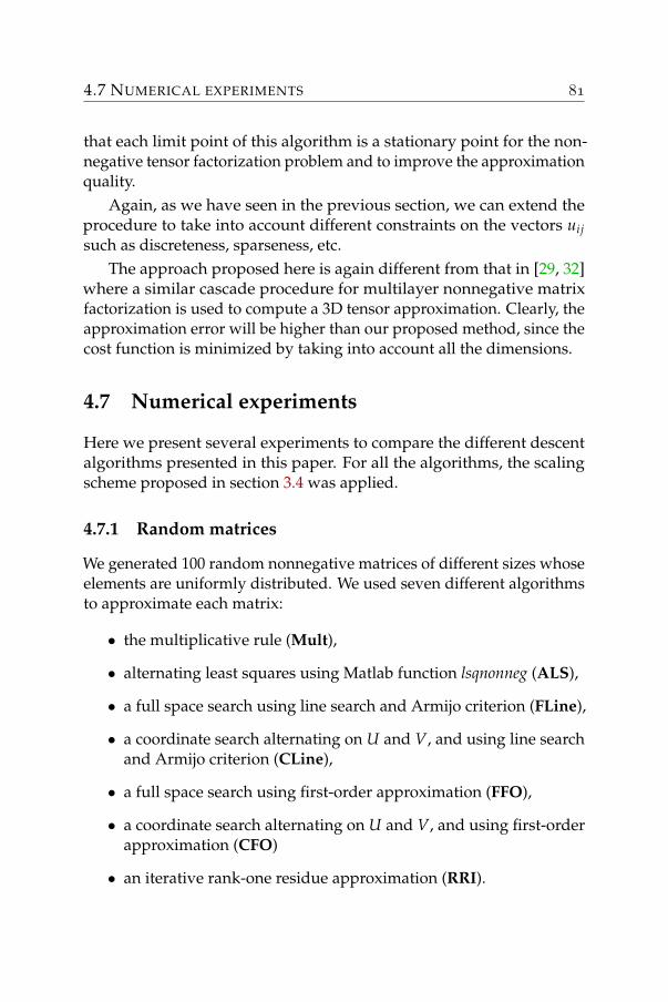
4.7 NUMERICAL EXPERIMENTS
that each limit point of this algorithm is a stationary point for the non-negative tensor factorization problem and to improve the approximationquality.
Again, as we have seen in the previous section, we can extend theprocedure to take into account different constraints on the vectors uijsuch as discreteness, sparseness, etc.
The approach proposed here is again different from that in [29, 32]where a similar cascade procedure for multilayer nonnegative matrixfactorization is used to compute a 3D tensor approximation. Clearly, theapproximation error will be higher than our proposed method, since thecost function is minimized by taking into account all the dimensions.
4.7 Numerical experiments
Here we present several experiments to compare the different descentalgorithms presented in this paper. For all the algorithms, the scalingscheme proposed in section 3.4 was applied.
4.7.1 Random matrices
We generated 100 random nonnegative matrices of different sizes whoseelements are uniformly distributed. We used seven different algorithmsto approximate each matrix:
• the multiplicative rule (Mult),
• alternating least squares using Matlab function lsqnonneg (ALS),
• a full space search using line search and Armijo criterion (FLine),
• a coordinate search alternating on U and V, and using line searchand Armijo criterion (CLine),
• a full space search using first-order approximation (FFO),
• a coordinate search alternating on U and V, and using first-orderapproximation (CFO)
• an iterative rank-one residue approximation (RRI).

RANK-ONE RESIDUE ITERATION
Table 4.1: Comparison of algorithms: Time limit is 45 seconds. The given figuresare the average successful running time over 100 random matrices. The figure0.02 (96) means that the algorithm returns a result with the required precision εwithin 45 seconds for only 96 (of 100) test matrices of which the average runningtime is 0.02 seconds. 45 ∗ (0) means that the algorithm fails in all 100 matrices.
Mult ALS FLine CLine FFO CFO RRI(m=30, n=20, r=2)
ε=10−2 0.02 0.40 0.04 0.02 0.02 0.01 0.01
(96)
ε=10−3 0.08 1.36 0.12 0.09 0.05 0.04 0.03
(74)
ε=10−4 0.17 2.81 0.24 0.17 0.11 0.08 0.05
(71)
ε=10−5 0.36 4.10 0.31 0.25 0.15 0.11 0.07
(64)
ε=10−6 0.31 4.74 0.40 0.29 0.19 0.15 0.09
(76)
(m=100, n=50, r=5)
ε=10−2 45∗ 3.48 0.10 0.09 0.09 0.04 0.02
(0)
ε=10−3 45∗ 24.30 0.59 0.63 0.78 0.25 0.15
(0) (96)
ε=10−4 45∗ 45∗ 2.74 2.18 3.34 0.86 0.45
(0) (0)
ε=10−5 45∗ 45∗ 5.93 4.06 6.71 1.58 0.89
(0) (0)
ε=10−6 45∗ 45∗ 7.23 4.75 8.98 1.93 1.30
(0) (0)
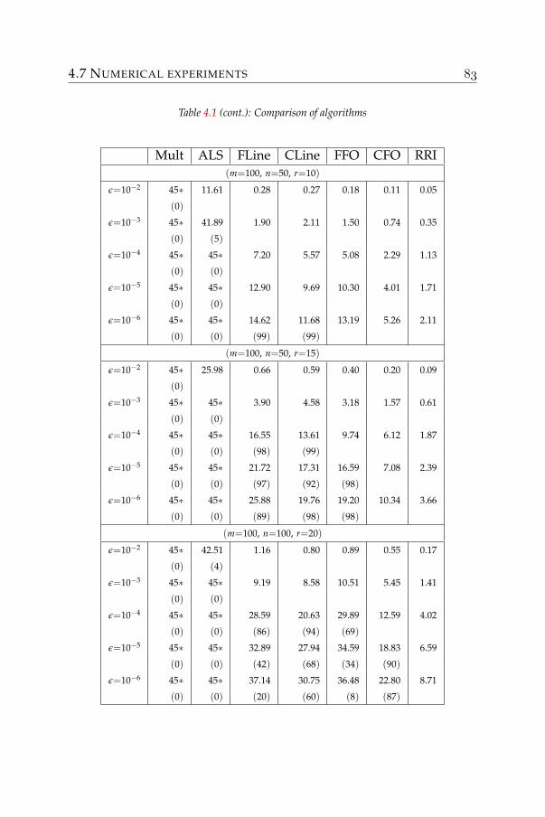
4.7 NUMERICAL EXPERIMENTS
Table 4.1 (cont.): Comparison of algorithms
Mult ALS FLine CLine FFO CFO RRI(m=100, n=50, r=10)
ε=10−2 45∗ 11.61 0.28 0.27 0.18 0.11 0.05
(0)
ε=10−3 45∗ 41.89 1.90 2.11 1.50 0.74 0.35
(0) (5)
ε=10−4 45∗ 45∗ 7.20 5.57 5.08 2.29 1.13
(0) (0)
ε=10−5 45∗ 45∗ 12.90 9.69 10.30 4.01 1.71
(0) (0)
ε=10−6 45∗ 45∗ 14.62 11.68 13.19 5.26 2.11
(0) (0) (99) (99)
(m=100, n=50, r=15)
ε=10−2 45∗ 25.98 0.66 0.59 0.40 0.20 0.09
(0)
ε=10−3 45∗ 45∗ 3.90 4.58 3.18 1.57 0.61
(0) (0)
ε=10−4 45∗ 45∗ 16.55 13.61 9.74 6.12 1.87
(0) (0) (98) (99)
ε=10−5 45∗ 45∗ 21.72 17.31 16.59 7.08 2.39
(0) (0) (97) (92) (98)
ε=10−6 45∗ 45∗ 25.88 19.76 19.20 10.34 3.66
(0) (0) (89) (98) (98)
(m=100, n=100, r=20)
ε=10−2 45∗ 42.51 1.16 0.80 0.89 0.55 0.17
(0) (4)
ε=10−3 45∗ 45∗ 9.19 8.58 10.51 5.45 1.41
(0) (0)
ε=10−4 45∗ 45∗ 28.59 20.63 29.89 12.59 4.02
(0) (0) (86) (94) (69)
ε=10−5 45∗ 45∗ 32.89 27.94 34.59 18.83 6.59
(0) (0) (42) (68) (34) (90)
ε=10−6 45∗ 45∗ 37.14 30.75 36.48 22.80 8.71
(0) (0) (20) (60) (8) (87)
RANK-ONE RESIDUE ITERATION
Table 4.1 (cont.): Comparison of algorithms
Mult ALS FLine CLine FFO CFO RRI(m=200, n=100, r=30)
ε=10−2 45∗ 45∗ 2.56 2.20 2.68 1.31 0.44
(0) (0)
ε=10−3 45∗ 45∗ 22.60 25.03 29.67 12.94 4.12
(0) (0) (99) (98) (90)
ε=10−4 45∗ 45∗ 36.49 39.13 45∗ 33.33 14.03
(0) (0) (2) (13) (0) (45)
ε=10−5 45∗ 45∗ 45∗ 39.84 45∗ 37.60 21.96
(0) (0) (0) (2) (0) (6) (92)
ε=10−6 45∗ 45∗ 45∗ 45∗ 45∗ 45∗ 25.61
(0) (0) (0) (0) (0) (0) (87)
(m=200, n=200, r=30)
ε=10−2 45∗ 45∗ 2.42 1.74 5.22 2.02 0.65
(0) (0)
ε=10−3 45∗ 45∗ 27.64 20.08 41.48 22.25 6.17
(0) (0) (99) (15)
ε=10−4 45∗ 45∗ 45∗ 45∗ 45∗ 45∗ 25.10
(0) (0) (0) (0) (0) (0) (90)
ε=10−5 45∗ 45∗ 45∗ 45∗ 45∗ 45∗ 30.42
(0) (0) (0) (0) (0) (0) (51)
ε=10−6 45∗ 45∗ 45∗ 45∗ 45∗ 45∗ 33.85
(0) (0) (0) (0) (0) (0) (32)
4.7 NUMERICAL EXPERIMENTS
For each matrix, the same starting point is used for every algorithm.We create a starting point by randomly generating two matrices U andV and then rescaling them to yield a first approximation of the originalmatrix A as proposed in Section 3.4:
U = UD√
α, V = VD−1√α,
where
α :=⟨
A, UVT⟩〈UVT, UVT〉 and Dij =
√‖V:i‖2‖U:i‖2
if i = j0 otherwise
.
The algorithms are all stopped when the projected gradient norm islower than ε times the gradient norm at the starting point or when ittakes more than 45 seconds. The relative precisions ε are chosen equal to10−2, 10−3, 10−4, 10−5, 10−6, 10−6. No limit was imposed on the numberof iterations.
For alternating gradient algorithms CLine and CFO, we use differentprecisions εU and εV for each of the inner iteration for U and for V assuggested in [86] where εU and εV are initialized by 10−3. And when theinner loop for U or V needs no iteration to reach the precision εU or εV ,one more digit of precision will be added into εU or εV (i.e. εU = εU/10or εV = εV/10).
Table 4.1 shows that for all sizes and ranks, Algorithm RRI is thefastest to reach the required precision. Even though it is widely used inpractice, algorithm Mult fails to provide solutions to the NMF problemwithin the allocated time. A further investigation shows that the algo-rithm gets easily trapped in boundary points where some Uij and/orVij is zero while ∇Uij and/or ∇Vij is negative, hence violating one of theKKT conditions (2.5). The multiplicative rules then fail to move anddo not return to a local minimizer. A slightly modified version of thisalgorithm was given in [85], but it needs to wait to get sufficiently closeto such points before attempting an escape, and is therefore also notefficient. The ALS algorithm can return a stationary point, but it takestoo long.
We select five methods: FLine, CLine, FFO, CFO and RRI for amore detailed comparison. For each matrix A, we run these algorithmswith 100 different starting points. Figure 4.1, 4.2, 4.3 and 4.4 show
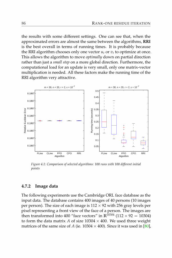
RANK-ONE RESIDUE ITERATION
the results with some different settings. One can see that, when theapproximated errors are almost the same between the algorithms, RRIis the best overall in terms of running times. It is probably becausethe RRI algorithm chooses only one vector ut or vt to optimize at once.This allows the algorithm to move optimally down on partial directionrather than just a small step on a more global direction. Furthermore, thecomputational load for an update is very small, only one matrix-vectormultiplication is needed. All these factors make the running time of theRRI algorithm very attractive.
FLine CLine FFO CFO RRI
0.1867
0.1867
0.1867
0.1867
0.1867
0.1867
0.1867
0.1867
Rel
ativ
e E
uclid
ean
Err
or
Algorithm
m = 30, n = 20, r = 2, ε = 10−7
FLine CLine FFO CFO RRI
0.05
0.1
0.15
0.2
0.25
0.3
0.35
0.4
0.45
0.5R
unni
ng ti
me
(sec
onds
)
Algorithm
m = 30, n = 20, r = 2, ε = 10−7
Figure 4.1: Comparison of selected algorithms: 100 runs with 100 different initialpoints
4.7.2 Image data
The following experiments use the Cambridge ORL face database as theinput data. The database contains 400 images of 40 persons (10 imagesper person). The size of each image is 112× 92 with 256 gray levels perpixel representing a front view of the face of a person. The images arethen transformed into 400 “face vectors” in R10304 (112× 92 = 10304)to form the data matrix A of size 10304× 400. We used three weightmatrices of the same size of A (ie. 10304× 400). Since it was used in [80],
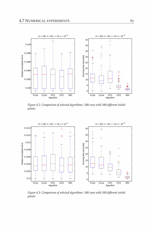
4.7 NUMERICAL EXPERIMENTS
FLine CLine FFO CFO RRI
0.148
0.1482
0.1484
0.1486
0.1488
0.149
Rel
ativ
e E
uclid
ean
Err
or
Algorithm
m = 100, n = 50, r = 10, ε = 10−5
FLine CLine FFO CFO RRI
0
5
10
15
20
25
30
35
40
45
Run
ning
tim
e (s
econ
ds)
Algorithm
m = 100, n = 50, r = 10, ε = 10−5
Figure 4.2: Comparison of selected algorithms: 100 runs with 100 different initialpoints
FLine CLine FFO CFO RRI
0.12
0.1202
0.1204
0.1206
0.1208
0.121
0.1212
0.1214
Rel
ativ
e E
uclid
ean
Err
or
Algorithm
m = 100, n = 50, r = 15, ε = 10−4
FLine CLine FFO CFO RRI
0
5
10
15
20
25
30
35
40
Run
ning
tim
e (s
econ
ds)
Algorithm
m = 100, n = 50, r = 15, ε = 10−4
Figure 4.3: Comparison of selected algorithms: 100 runs with 100 different initialpoints
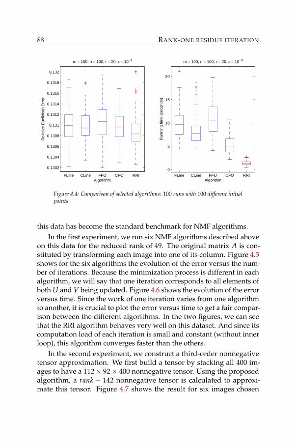
RANK-ONE RESIDUE ITERATION
FLine CLine FFO CFO RRI
0.1302
0.1304
0.1306
0.1308
0.131
0.1312
0.1314
0.1316
0.1318
0.132
Rel
ativ
e E
uclid
ean
Err
or
Algorithm
m = 100, n = 100, r = 20, ε = 10−3
FLine CLine FFO CFO RRI0
5
10
15
20
Run
ning
tim
e (s
econ
ds)
Algorithm
m = 100, n = 100, r = 20, ε = 10−3
Figure 4.4: Comparison of selected algorithms: 100 runs with 100 different initialpoints
this data has become the standard benchmark for NMF algorithms.In the first experiment, we run six NMF algorithms described above
on this data for the reduced rank of 49. The original matrix A is con-stituted by transforming each image into one of its column. Figure 4.5shows for the six algorithms the evolution of the error versus the num-ber of iterations. Because the minimization process is different in eachalgorithm, we will say that one iteration corresponds to all elements ofboth U and V being updated. Figure 4.6 shows the evolution of the errorversus time. Since the work of one iteration varies from one algorithmto another, it is crucial to plot the error versus time to get a fair compar-ison between the different algorithms. In the two figures, we can seethat the RRI algorithm behaves very well on this dataset. And since itscomputation load of each iteration is small and constant (without innerloop), this algorithm converges faster than the others.
In the second experiment, we construct a third-order nonnegativetensor approximation. We first build a tensor by stacking all 400 im-ages to have a 112× 92× 400 nonnegative tensor. Using the proposedalgorithm, a rank − 142 nonnegative tensor is calculated to approxi-mate this tensor. Figure 4.7 shows the result for six images chosen
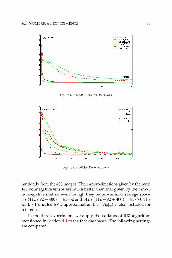
4.7 NUMERICAL EXPERIMENTS
Figure 4.5: NMF: Error vs. Iterations
Figure 4.6: NMF: Error vs. Time
randomly from the 400 images. Their approximations given by the rank-142 nonnegative tensor are much better than that given by the rank-8nonnegative matrix, even though they require similar storage space:8 ∗ (112 ∗ 92 + 400) = 85632 and 142 ∗ (112 + 92 + 400) = 85768. Therank-8 truncated SVD approximation (i.e. [A8]+) is also included forreference.
In the third experiment, we apply the variants of RRI algorithmmentioned in Section 4.4 to the face databases. The following settingsare compared:

RANK-ONE RESIDUE ITERATION
Figure 4.7: Tensor Factorization vs. Matrix Factorization on facial data. Sixrandomly chosen images from 400 of ORL dataset. From top to bottom: originalimages, their rank− 142 nonnegative tensor approximation, their rank− 8 trun-cated SVD approximation and their rank− 8 nonnegative matrix approximation.
• Original: original faces from the databases.
• 49NMF: standard factorization (nonnegative vectors), r = 49.
• 100Binary: columns of U are limited to the scaled binary vectors,r = 100.
• 49Sparse10: columns of U are sparse. Not more than 10% of theelements of each column of A are positive. r = 49.
• 49Sparse20: columns of U are sparse. Not more than 20% of theelements of each column of A are positive. r = 49.
• 49HSparse60: columns of U are sparse. The Hoyer sparsity ofeach column of U are 0.6. r = 49.
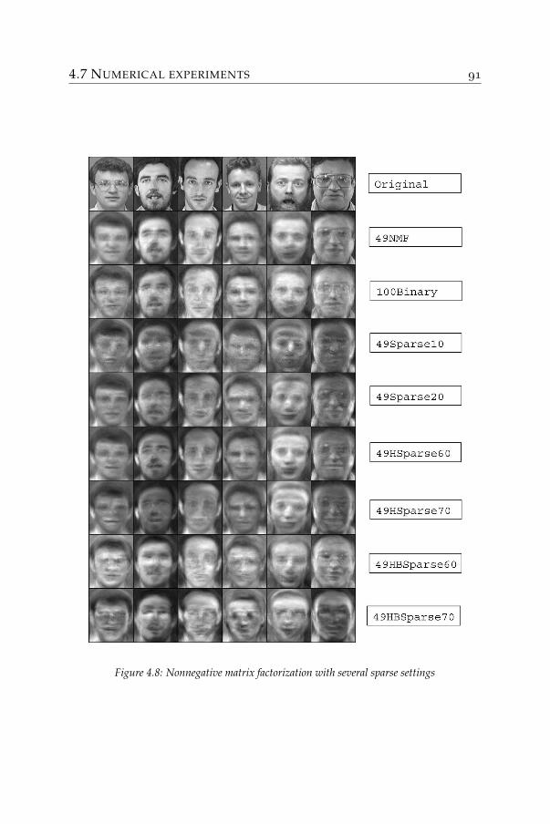
4.7 NUMERICAL EXPERIMENTS
Figure 4.8: Nonnegative matrix factorization with several sparse settings
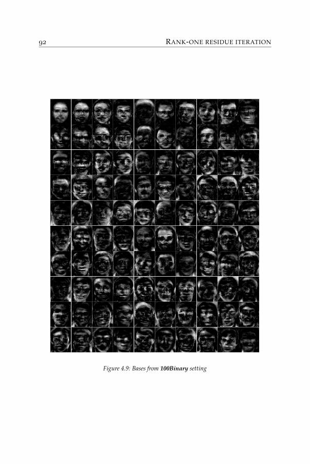
RANK-ONE RESIDUE ITERATION
Figure 4.9: Bases from 100Binary setting
4.7 NUMERICAL EXPERIMENTS
• 49HSparse70: columns of U are sparse. The Hoyer sparsity ofeach column of U are 0.7. r = 49.
• 49HBSparse60: columns of U are sparse. The Hoyer sparsity ofeach column of U are 0.6. Columns of V are scaled binary. r = 49.
• 49HBSparse70: columns of U are sparse. The Hoyer sparsity ofeach column of U are 0.7. Columns of V are scaled binary. r = 49.
For each setting, we use RRI algorithm to compute the correspondingfactorization. Some randomly selected faces are reconstructed by thesesettings as shown in Figure 4.8. For each setting, RRI algorithm producesa different set of bases to approximate the original faces. When thecolumns of V are constrained to scaled binary vectors (100Binary), thefactorization can be rewritten as UVT = UBT, where B is a binary matrix.This implies that each image is reconstructed by just the presence orabsence of 100 bases shown in Figure 4.9.
Figure 4.10 and 4.11 show nonnegative bases obtained by imposingsome sparsity on the columns of V. The sparsity can be easily con-trolled by the percentages of positive elements or by the Hoyer sparsitymeasure.
Figure 4.12 combines the sparsity of the bases (columns of U) andthe binary representation of V. The sparsity is measured by he Hoyermeasure as in Figure 4.11. Only with the absence or presence of these 49features, faces are approximated as shown in the last two rows of Figure4.8.
The above examples show how to use the variants of the RRI algo-rithm to control the sparsity of the bases. One can see that the sparserthe bases are, the less storage is needed to store the approximation.Moreover, this provides a part-based decomposition using local featuresof the faces.
4.7.3 Smooth approximation
We carry out this experiment to test the new smoothness constraintintroduced in the previous section:
12‖Ri − uivT‖2
F +δ
2‖v− Bvi‖2
F, δ > 0
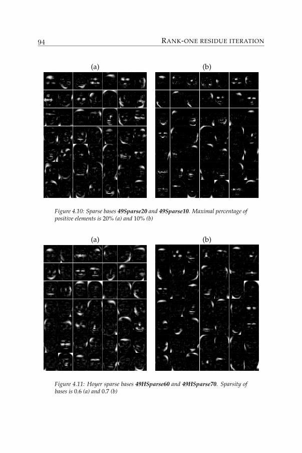
RANK-ONE RESIDUE ITERATION
(a) (b)
Figure 4.10: Sparse bases 49Sparse20 and 49Sparse10. Maximal percentage ofpositive elements is 20% (a) and 10% (b)
(a) (b)
Figure 4.11: Hoyer sparse bases 49HSparse60 and 49HSparse70. Sparsity ofbases is 0.6 (a) and 0.7 (b)
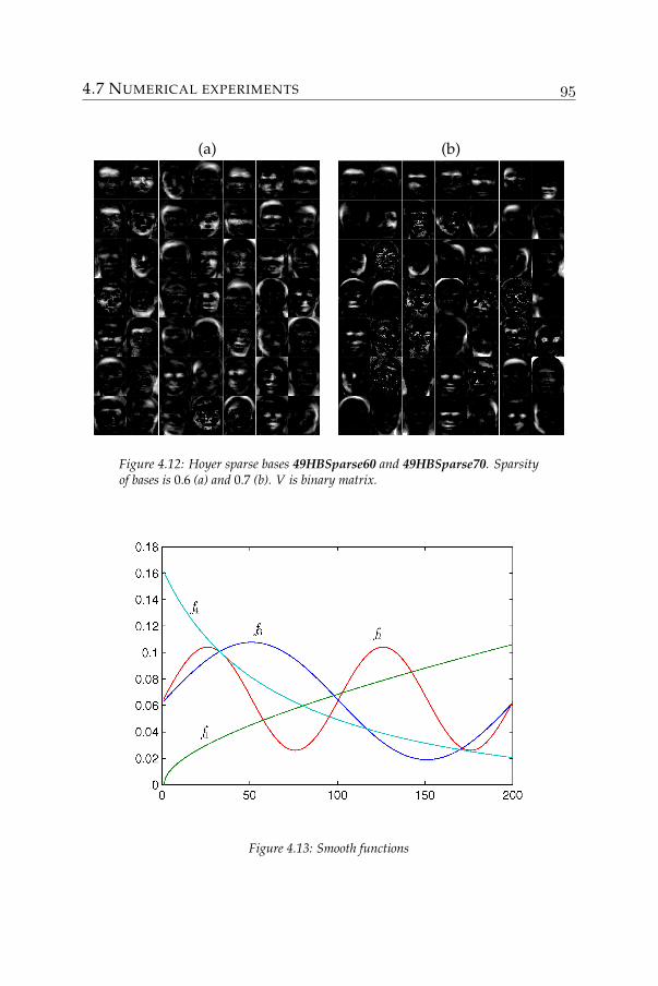
4.7 NUMERICAL EXPERIMENTS
(a) (b)
Figure 4.12: Hoyer sparse bases 49HBSparse60 and 49HBSparse70. Sparsityof bases is 0.6 (a) and 0.7 (b). V is binary matrix.
Figure 4.13: Smooth functions
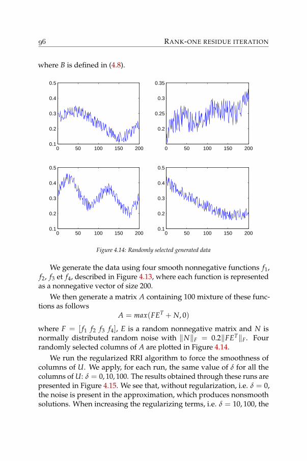
RANK-ONE RESIDUE ITERATION
where B is defined in (4.8).
0 50 100 150 2000.1
0.2
0.3
0.4
0.5
0 50 100 150 200
0.2
0.25
0.3
0.35
0 50 100 150 2000.1
0.2
0.3
0.4
0.5
0 50 100 150 2000.1
0.2
0.3
0.4
0.5
Figure 4.14: Randomly selected generated data
We generate the data using four smooth nonnegative functions f1,f2, f3 et f4, described in Figure 4.13, where each function is representedas a nonnegative vector of size 200.
We then generate a matrix A containing 100 mixture of these func-tions as follows
A = max(FET + N, 0)
where F = [ f1 f2 f3 f4], E is a random nonnegative matrix and N isnormally distributed random noise with ‖N‖F = 0.2‖FET‖F. Fourrandomly selected columns of A are plotted in Figure 4.14.
We run the regularized RRI algorithm to force the smoothness ofcolumns of U. We apply, for each run, the same value of δ for all thecolumns of U: δ = 0, 10, 100. The results obtained through these runs arepresented in Figure 4.15. We see that, without regularization, i.e. δ = 0,the noise is present in the approximation, which produces nonsmoothsolutions. When increasing the regularizing terms, i.e. δ = 10, 100, the
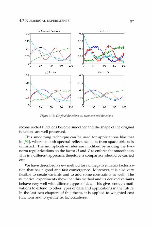
4.7 NUMERICAL EXPERIMENTS
Figure 4.15: Original functions vs. reconstructed functions
reconstructed functions become smoother and the shape of the originalfunctions are well preserved.
This smoothing technique can be used for applications like thatin [99], where smooth spectral reflectance data from space objects isunmixed. The multiplicative rules are modified by adding the two-norm regularizations on the factor U and V to enforce the smoothness.This is a different approach, therefore, a comparison should be carriedout.
We have described a new method for nonnegative matrix factoriza-tion that has a good and fast convergence. Moreover, it is also veryflexible to create variants and to add some constraints as well. Thenumerical experiments show that this method and its derived variantsbehave very well with different types of data. This gives enough moti-vations to extend to other types of data and applications in the future.In the last two chapters of this thesis, it is applied to weighted costfunctions and to symmetric factorizations.

RANK-ONE RESIDUE ITERATION
5
NONNEGATIVE MATRIXFACTORIZATION WITH FIXED ROW
AND COLUMN SUMS
An important class of nonnegative matrices are stochastic matrices.Typical applications of this are PageRank [23] used for ordering the webpages, Markov Clustering [117] used for clustering vertices in a graphand Hidden Markov Models [100] used for learning and predictingsequential data. The number of such applications is growing, but thesize of the underlying problems is growing as well. The size of thestochastic matrices representing Markov chains related to the web is e.g.of the order of billions. In order to cope with such large-scale stochasticmatrices, one could use NMF to approximate a large stochastic matrixby a lower-rank one.
We will begin with the introduction of the problem. We will showthat the constraint under which the row and column sums are preservedis automatically satisfied by using the generalized Kullback-Leibler di-vergence as the cost function for the NMF problem. In [42], a discussionis made leading to the preservation of the matrix sum when using thegeneralized Kullback-Leibler divergence in the NMF. But this is just astraightforward result from the preservation of row and column sums,which will be pointed out.
NMF WITH FIXED ROW AND COLUMN SUMS
5.1 Problem statement
The general NMF problem with preserved column and row sums isdescribed as follows:
Problem 5.1 (NMF with preserved column and row sums). Given am× n nonnegative matrix A, solve
minU∈Rm×r
+ V∈Rn×r
UVT1n×1=A1n×1VUT1m×1=AT1m×1
F(A, UVT)
where F(A, UVT) is the chosen “distance” function.
The additional constraints are linear in each factor U or V (not onboth). In fact, fixing for example U, they are linear on V. To see that theyare not convex on both U and V, taking two feasible points, i.e. (U1, V1)and (U2, V2), their convex combinations α(U1, V1) + (1 − α)(U2, V2),with α ∈ (0, 1) are, in general, not in the feasible set. When F is theEuclidean distance, one can use alternating minimizations to solve thisproblem, since the problem is convex in each of the factors U and V.
If we partition the variables as suggested in Chapter 4 and fix allthe variables ui’s and vi’s except for one vk, then the feasible set of vkcontains at most one element and could be empty. This means that wecan not modify one variable without modifying the others while stayingin the feasible set. In fact, the set of m× n rank-one nonnegative matrixwith predefined nonnegative row and column sums is very simple. Letr and c be the vector of row sums and column sums respectively anduvT is a candidate rank-one matrix. From the sum constraints we have:
uvT1n×1 = u‖v‖1 = r
andvuT1m×1 = v‖u‖1 = c,
or u and v are parallel to r and c. Moreover,
(1Tn×1uvT1n×1) = ‖u‖1‖v‖1 = rT1n×1 = 1T
n×1c
5.1 PROBLEM STATEMENT
we have uvT = rcT
‖c‖1. This implies that the rank-one solution to Problem
5.1 is independent of the choice of cost measure and is always
(u, v) =1‖c‖1
(αr,1α
c) with α > 0.
For higher ranks, one could eliminate these sum constraints byrewriting a chosen variable pair (uk, vk) as a function of other vari-ables. But this makes the cost function really complicated to analyze. Inthis case, one might better use a generic optimization tool.
In the context of nonnegative matrix with predefined row and col-umn sums, the Sinkhorn algorithm [107] is well-known for the diagonalscaling problem: given a nonnegative square matrix A and two nonneg-ative vectors r and c (∑i ri = ∑i ci), finding two positive diagonal matrixD1 and D2 with appropriate size such that the scaled matrix B = D1AD2satisfies B1 = r and BT1 = c. This means that the scaled matrix has cand r as the vectors of column sums and row sums, respectively. Theprocess is very simple and consists of alternatively scaling the rows andcolumns of A. A necessary and sufficient condition for the convergencewas also given by the author.
When the Sinkhorn algorithm converges, it produces a matrix B withthe predefined row sums r and column sums c. It was shown in [71]that, among matrices with the predefined row sums r and column sumsc, B is the closest to A with respect to the generalized Kullback-Leiblerdivergence:
D(B‖A) = ∑ij
[Bij log
Bij
Aij− Bij + Aij
], (5.1)
where by convention, we put 00 = 0 and 0log0 = 0. Moreover, given a
matrix A and vectors r and c, B is unique.The Kullback-Leibler divergence [78] is well-known in probability
theory and information theory. It is also known as information divergence,information gain or relative entropy, that measures the difference betweentwo probability distributions. Its generalized version above measuresthe difference between two nonnegative vectors, which is an instanceof the Bregman divergences, see for example [91]. These divergencesare similar to a distance but do not satisfy the triangle inequality nor
NMF WITH FIXED ROW AND COLUMN SUMS
symmetry, except for Euclidean Distance, an important element of theclass.
We will show that, when using this measure to approximate a non-negative matrix, the row and column sums of the input matrix will beretained in the low-rank approximation. Note that the use of the general-ized Kullback-Leibler divergence in the diagonal scaling problem aboveand the problem in the next section are different. For the earlier, the in-put matrix is the second parameter of the divergence, i.e. D(.‖A). Whileit is the second parameter, i.e. D(A‖.), in the nonnegative matrix factor-ization with the generalized Kullback-Leibler divergence, described inthis chapter.
5.2 Generalized KL divergence in NMF
In this section, we focus on the use of the generalized Kullback-Leibler(KL) divergence in the problem of nonnegative matrix factorization. Wewill show that when using the generalized KL divergence as the costfunction for NMF, row sums and column sums of the original matrix arepreserved in the approximation. We will use this special characteristicin several approximation problems.
It is known that the generalized Kullback-Leibler divergence (5.1)is always nonnegative and zero if and only if B = A, [91]. It is notsymmetric, i.e. D(A‖B) 6= D(B‖A) and does not satisfy the triangleequation. Figures 5.1 and 5.2 show the level sets of two measuresD(x‖(2, 5)) and D((2, 5)‖x).
5.2.1 Row and column sums preserving approximation
The choice of cost function F of course affects the solution of the mini-mization problem. The nonnegative matrix factorization problem withthe generalized Kullback-Leibler divergence as the new cost function is
minU+∈Rm×r V+∈Rn×r
D(A‖UVT) (5.2)
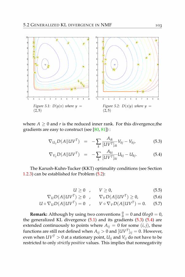
5.2 GENERALIZED KL DIVERGENCE IN NMF
0.1
1
12
2
3
3
4
4
5
5
5
6
6
6
7
7
8
8
9
9
10
10
y
−1 0 1 2 3 4 5 6 7 8 9 10−1
0
1
2
3
4
5
6
7
8
9
10
Figure 5.1: D(y|x) where y =(2, 5)
0.1
11
2
2
3
3
4
4
5
5
6
6
7
78
8
9
9
9
10
10
y
−1 0 1 2 3 4 5 6 7 8 9 10−1
0
1
2
3
4
5
6
7
8
9
10
Figure 5.2: D(x|y) where y =(2, 5)
where A ≥ 0 and r is the reduced inner rank. For this divergence,thegradients are easy to construct (see [80, 81]) :
∇Uij D(A‖UVT) = −∑k
Aik
[UVT]ikVkj −Vkj, (5.3)
∇Vij D(A‖UVT) = −∑k
Aki
[UVT]kiUkj −Ukj. (5.4)
The Karush-Kuhn-Tucker (KKT) optimality conditions (see Section1.2.3) can be established for Problem (5.2):
U ≥ 0 , V ≥ 0, (5.5)∇U D(A‖UVT) ≥ 0 , ∇V D(A‖UVT) ≥ 0, (5.6)
U ∇U D(A‖UVT) = 0 , V ∇V D(A‖UVT) = 0. (5.7)
Remark: Although by using two conventions 00 = 0 and 0log0 = 0,
the generalized KL divergence (5.1) and its gradients (5.3) (5.4) areextended continuously to points where Aij = 0 for some (i, j), thesefunctions are still not defined when Aij > 0 and [UVT]ij = 0. However,even when UVT > 0 at a stationary point, Uij and Vij do not have to berestricted to only strictly positive values. This implies that nonnegativity
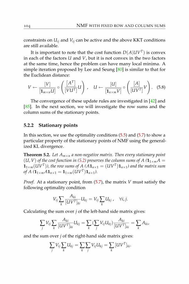
NMF WITH FIXED ROW AND COLUMN SUMS
constraints on Uij and Vij can be active and the above KKT conditionsare still available.
It is important to note that the cost function D(A|UVT) is convexin each of the factors U and V, but it is not convex in the two factorsat the same time, hence the problem can have many local minima. Asimple iteration proposed by Lee and Seung [80] is similar to that forthe Euclidean distance:
V ← [V][1m×nU]
( [
AT][VUT]
U
), U ← [U]
[1n×mV](
[A][UVT]
V
). (5.8)
The convergence of these update rules are investigated in [42] and[85]. In the next section, we will investigate the row sums and thecolumn sums of the stationary points.
5.2.2 Stationary points
In this section, we use the optimality conditions (5.5) and (5.7) to show aparticular property of the stationary points of NMF using the general-ized KL divergence.
Theorem 5.2. Let Am×n a non-negative matrix. Then every stationary point(U, V) of the cost function in (5.2) preserves the column sums of A (11×m A =11×m(UVT)), the row sums of A (A1n×1 = (UVT)1n×1) and the matrix sumof A (11×m A1n×1 = 11×m(UVT)1n×1).
Proof. At a stationary point, from (5.7), the matrix V must satisfy thefollowing optimality condition
Vij ∑k
Aki
[UVT]kiUkj = Vij ∑
kUkj , ∀i, j.
Calculating the sum over j of the left-hand side matrix gives:
∑j
Vij ∑k
Aki
[UVT]kiUkj = ∑
k(∑
jVijUkj)
Aki
[UVT]ki= ∑
kAki,
and the sum over j of the right-hand side matrix gives:
∑j
Vij ∑k
Ukj = ∑k
∑j
VijUkj = ∑k
[UVT]ki.
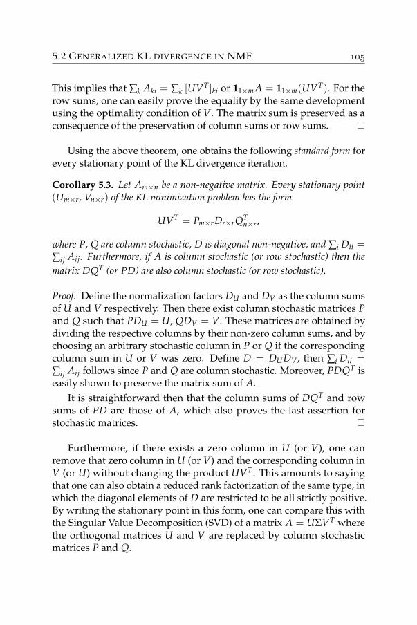
5.2 GENERALIZED KL DIVERGENCE IN NMF
This implies that ∑k Aki = ∑k [UVT]ki or 11×m A = 11×m(UVT). For therow sums, one can easily prove the equality by the same developmentusing the optimality condition of V. The matrix sum is preserved as aconsequence of the preservation of column sums or row sums.
Using the above theorem, one obtains the following standard form forevery stationary point of the KL divergence iteration.
Corollary 5.3. Let Am×n be a non-negative matrix. Every stationary point(Um×r, Vn×r) of the KL minimization problem has the form
UVT = Pm×rDr×rQTn×r,
where P, Q are column stochastic, D is diagonal non-negative, and ∑i Dii =∑ij Aij. Furthermore, if A is column stochastic (or row stochastic) then thematrix DQT (or PD) are also column stochastic (or row stochastic).
Proof. Define the normalization factors DU and DV as the column sumsof U and V respectively. Then there exist column stochastic matrices Pand Q such that PDU = U, QDV = V. These matrices are obtained bydividing the respective columns by their non-zero column sums, and bychoosing an arbitrary stochastic column in P or Q if the correspondingcolumn sum in U or V was zero. Define D = DU DV , then ∑i Dii =∑ij Aij follows since P and Q are column stochastic. Moreover, PDQT iseasily shown to preserve the matrix sum of A.
It is straightforward then that the column sums of DQT and rowsums of PD are those of A, which also proves the last assertion forstochastic matrices.
Furthermore, if there exists a zero column in U (or V), one canremove that zero column in U (or V) and the corresponding column inV (or U) without changing the product UVT. This amounts to sayingthat one can also obtain a reduced rank factorization of the same type, inwhich the diagonal elements of D are restricted to be all strictly positive.By writing the stationary point in this form, one can compare this withthe Singular Value Decomposition (SVD) of a matrix A = UΣVT wherethe orthogonal matrices U and V are replaced by column stochasticmatrices P and Q.
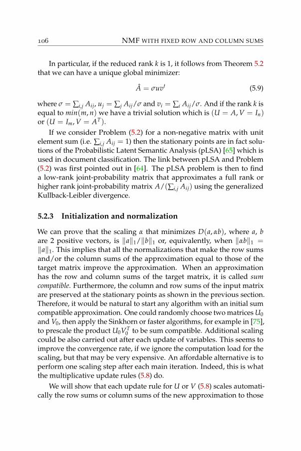
NMF WITH FIXED ROW AND COLUMN SUMS
In particular, if the reduced rank k is 1, it follows from Theorem 5.2that we can have a unique global minimizer:
A = σuvt (5.9)
where σ = ∑i,j Aij, uj = ∑j Aij/σ and vi = ∑i Aij/σ. And if the rank k isequal to min(m, n) we have a trivial solution which is (U = A, V = In)or (U = Im, V = AT).
If we consider Problem (5.2) for a non-negative matrix with unitelement sum (i.e. ∑i,j Aij = 1) then the stationary points are in fact solu-tions of the Probabilistic Latent Semantic Analysis (pLSA) [65] which isused in document classification. The link between pLSA and Problem(5.2) was first pointed out in [64]. The pLSA problem is then to finda low-rank joint-probability matrix that approximates a full rank orhigher rank joint-probability matrix A/(∑i,j Aij) using the generalizedKullback-Leibler divergence.
5.2.3 Initialization and normalization
We can prove that the scaling α that minimizes D(a, αb), where a, bare 2 positive vectors, is ‖a‖1/‖b‖1 or, equivalently, when ‖αb‖1 =‖a‖1. This implies that all the normalizations that make the row sumsand/or the column sums of the approximation equal to those of thetarget matrix improve the approximation. When an approximationhas the row and column sums of the target matrix, it is called sumcompatible. Furthermore, the column and row sums of the input matrixare preserved at the stationary points as shown in the previous section.Therefore, it would be natural to start any algorithm with an initial sumcompatible approximation. One could randomly choose two matrices U0and V0, then apply the Sinkhorn or faster algorithms, for example in [75],to prescale the product U0VT
0 to be sum compatible. Additional scalingcould be also carried out after each update of variables. This seems toimprove the convergence rate, if we ignore the computation load for thescaling, but that may be very expensive. An affordable alternative is toperform one scaling step after each main iteration. Indeed, this is whatthe multiplicative update rules (5.8) do.
We will show that each update rule for U or V (5.8) scales automati-cally the row sums or column sums of the new approximation to those
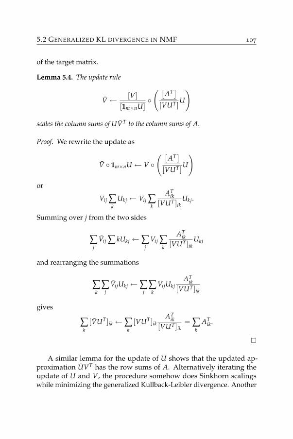
5.2 GENERALIZED KL DIVERGENCE IN NMF
of the target matrix.
Lemma 5.4. The update rule
V ← [V][1m×nU]
( [
AT][VUT]
U
)
scales the column sums of UVT to the column sums of A.
Proof. We rewrite the update as
V 1m×nU ← V ( [
AT][VUT]
U
)or
Vij ∑k
Ukj ← Vij ∑k
ATik
[VUT]ikUkj.
Summing over j from the two sides
∑j
Vij ∑ kUkj ←∑j
Vij ∑k
ATik
[VUT]ikUkj
and rearranging the summations
∑k
∑j
VijUkj ←∑j
∑k
VijUkjAT
ik[VUT]ik
gives
∑k
[VUT]ik ←∑k
[VUT]ikAT
ik[VUT]ik
= ∑k
ATik.
A similar lemma for the update of U shows that the updated ap-proximation UVT has the row sums of A. Alternatively iterating theupdate of U and V, the procedure somehow does Sinkhorn scalingswhile minimizing the generalized Kullback-Leibler divergence. Another
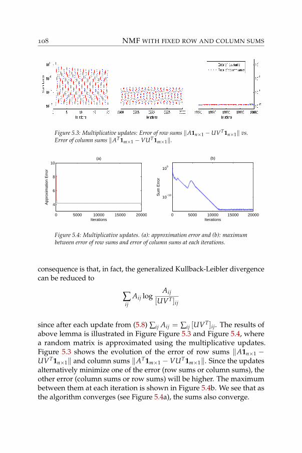
NMF WITH FIXED ROW AND COLUMN SUMS
Figure 5.3: Multiplicative updates: Error of row sums ‖A1n×1 −UVT1n×1‖ vs.Error of column sums ‖AT1m×1 −VUT1m×1‖.
0 5000 10000 15000 20000
4
6
8
10(a)
Iterations
App
roxi
mat
ion
Err
or
0 5000 10000 15000 20000
10−10
100
Iterations
Sum
Err
or(b)
Figure 5.4: Multiplicative updates. (a): approximation error and (b): maximumbetween error of row sums and error of column sums at each iterations.
consequence is that, in fact, the generalized Kullback-Leibler divergencecan be reduced to
∑ij
Aij logAij
[UVT]ij
since after each update from (5.8) ∑ij Aij = ∑ij [UVT]ij. The results ofabove lemma is illustrated in Figure Figure 5.3 and Figure 5.4, wherea random matrix is approximated using the multiplicative updates.Figure 5.3 shows the evolution of the error of row sums ‖A1n×1 −UVT1n×1‖ and column sums ‖AT1m×1 −VUT1m×1‖. Since the updatesalternatively minimize one of the error (row sums or column sums), theother error (column sums or row sums) will be higher. The maximumbetween them at each iteration is shown in Figure 5.4b. We see that asthe algorithm converges (see Figure 5.4a), the sums also converge.
5.3 APPLICATION: STOCHASTIC MATRIX APPROXIMATION
5.3 Application: stochastic matrix approximation
If the input matrix A is stochastic, the stochastic matrix UVT that min-imizes the generalized KL divergence is called a low-rank stochasticapproximation of A. Theorem 5.2 shows that if the input matrix A iscolumn stochastic (or row stochastic or doubly stochastic), the stationarypoints UVT are actually column stochastic (or row stochastic or doublystochastic). In other words, the stochasticity of the original matrix isnaturally preserved in the approximation.
Using the iterative algorithm in [81], one can numerically obtaina solution for the stochastic matrix approximation problem. Here aresome examples of stationary points that are candidates for a solution:
• column stochastic matrix
A =
12 0 1
212 0 00 1 1
2
≈ PDQT =
0 23
0 13
1 0
[ 32 00 3
2
] [0 2
313
23 0 1
3
],
(5.10)
• row stochastic matrix
A =
12 0 1
20 1
212
23
13 0
≈ PDQT (5.11)
=
0 35
34 014
25
[ 43 00 5
3
] [0 5
838
710 0 3
10
],
• and doubly stochastic
A =
38
14
38
14
12
14
38
14
38
= PDQT = PDPT (5.12)
=
12
14
0 12
12
14
[ 1 00 2
] [ 12 0 1
214
12
14
].
NMF WITH FIXED ROW AND COLUMN SUMS
In the above examples, the approximations are written in the formpresented in Corollary 5.3. Especially, in the third example of a doublystochastic matrix, we have an exact and symmetric factorization ofthe form PDPT. In general, it is not easy to find such a symmetricapproximation.
Furthermore, instead of considering the ordinary sum of a vector,we can consider the weighted sum of a vector x, defined as
sw(x) = ∑i
wixi = xTw (5.13)
where w is a positive weight vector. One can find an approximation thatpreserves the weighted column sums and row sums of the original ma-trix. In fact, suppose wr and wc are weight vectors with respect to whichwe want to find a low rank approximation UVT of A that preserves theweighted row sums and the weighted column sums respectively, i.e.
UVTwr = Awr wTc UVT = wT
c A, (5.14)
we can use the following procedure
1. Create A = Dwr ADwc ,
2. find a low rank non-negative approximation UVT of A by usingNMF algorithm for generalized KL divergence,
3. and create the desired approximation UVT where U = D−1wc
U andV = D−1
wrV.
Applying Theorem 5.2, one can easily check that (5.14) does hold forthe newly created matrix UVT.
The preservation of weighted column sums and row sums impliesthat we can use the same procedure to construct a low rank non-negativeapproximation that preserve the left and right principal eigenvectors ofa square non-negative matrix. The technique is then simply to use theleft and right principal eigenvectors of the original matrix as the weightvectors described above to construct the desired approximation.
6
WEIGHTS IN NONNEGATIVE MATRIXFACTORIZATION
A data matrix often comes from a data acquisition process. These pro-cesses are sometimes susceptible to the loss of precision or even to theabsence of some data. Therefore, when approximating such a matrix,more reliable elements should receive more attention. The reliability canbe simply a 0/1 representing the absence/presence of the data. But it isusually coded as a nonnegative number called the weight. The biggerthe weight is, the more important the element is.
In this chapter, we will investigate the problem of Weighted Nonnega-tive Matrix Factorization (WNMF) which minimize the Weighted EuclideanDistance:
12‖A−UVT‖2
W :=12 ∑
ij[W (A−UVT) (A−UVT)]ij (6.1)
where W = Wij ≥ 0 is a nonnegative weight matrix. Clearly, we canconsider the unweighted version as a particular case of the weightedone where all the elements of the weight matrix are equal to 1.
While extending the Euclidean Distance to the weighted case israther straightforward, the weighted approximation problem is muchmore difficult. Even when the nonnegativity constraints are omitted,an analytical solution no longer exists, except when the all-one weightmatrix is used. Numerical algorithms usually produce local minima[111].
The problem of Weighted Nonnegative Matrix Factorization was first
WEIGHTS IN NONNEGATIVE MATRIX FACTORIZATION
stated in [96] for the Weighted Euclidean Distance (6.1). Recently [53], aparticular type of weighting was proposed for the generalized Kullback-Leibler divergence as a cost function, in order to vary the importance ofeach column of the matrix A in the approximation UVD ≈ AD, whereD is a nonnegative diagonal scaling matrix. One can easily see that thisnonnegative weight matrix is equivalent to a rank-one weighting matrixW in our weighted formulation.
An approach that allows to use weight matrices in a more generalcontext is given in [111], where an Expectation-Maximization algorithmis used in an iterative scheme that produces an unweighted low-rankapproximation of a weighted combination of a previously computedapproximation :
(Uk+1, Vk+1) = LowRank(W A + (1−W) (UkVk)). (6.2)
Here there are no constraints of non-negativity, but the same idea canalso be used to incorporate weights in an algorithm for nonnegativematrix factorizations. This implies that one has to solve an unweightedlow-rank nonnegative approximation at each step of the iteration, andthis can become quite inefficient in terms of complexity.
The chapter begins with the gradient information of the weight Eu-clidean distance that every standard gradient method can use. Then wewill extend two particular methods: the multiplicative rules and Rank-one Residue Iteration to take into account the weight matrix. This isfollowed by a discussion about an interesting link between the weightedEuclidean distance and the weighted generalized Kullback-Leibler di-vergence in which the weighted multiplicative rules for the latter arealso derived. We will see next how the weight matrix can also be addedinto some existing NMF variants such as: Nonnegative Tensor Factor-ization, Nonnegative Matrix Factorization with Sparseness constraint,etc. The chapter will end with some numerical experiment on the imagedata of human faces where weights are used to emphasize meaningfulfeatures. Let us start with the gradient information.
6.1 Gradient information
We restate here the problem of Weighted Nonnegative Matrix Factoriza-tion:
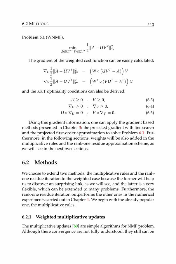
6.2 METHODS
Problem 6.1 (WNMF).
minU∈Rm×r
+ V∈Rn×r+
12‖A−UVT‖2
W .
The gradient of the weighted cost function can be easily calculated:
∇U12‖A−UVT‖2
W =(
W (UVT − A))
V
∇V12‖A−UVT‖2
W =(
WT (VUT − AT))
U
and the KKT optimality conditions can also be derived:
U ≥ 0 , V ≥ 0, (6.3)∇U ≥ 0 , ∇V ≥ 0, (6.4)
U ∇U = 0 , V ∇V = 0. (6.5)
Using this gradient information, one can apply the gradient basedmethods presented in Chapter 3: the projected gradient with line searchand the projected first-order approximation to solve Problem 6.1. Fur-thermore, in the following sections, weights will be also added in themultiplicative rules and the rank-one residue approximation scheme, aswe will see in the next two sections.
6.2 Methods
We choose to extend two methods: the multiplicative rules and the rank-one residue iteration to the weighted case because the former will helpus to discover an surprising link, as we will see, and the latter is a veryflexible, which can be extended to many problems. Furthermore, therank-one residue iteration outperforms the other ones in the numericalexperiments carried out in Chapter 4. We begin with the already popularone, the multiplicative rules.
6.2.1 Weighted multiplicative updates
The multiplicative updates [80] are simple algorithms for NMF problem.Although there convergence are not fully understood, they still can be
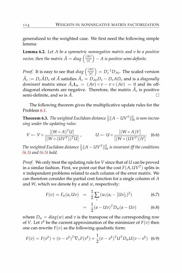
WEIGHTS IN NONNEGATIVE MATRIX FACTORIZATION
generalized to the weighted case. We first need the following simplelemma:
Lemma 6.2. Let A be a symmetric nonnegative matrix and v be a positive
vector, then the matrix A = diag( [Av]
[v]
)− A is positive semi-definite.
Proof. It is easy to see that diag( [Av]
[v]
)= D−1
v DAv. The scaled version
As := Dv ADv of A satisfies As = DAvDv − Dv ADv and is a diagonallydominant matrix since As1m = (Av) v − v (Av) = 0 and its off-diagonal elements are negative. Therefore, the matrix As is positivesemi-definite, and so is A.
The following theorem gives the multiplicative update rules for theProblem 6.1.
Theorem 6.3. The weighted Euclidean distance 12‖A−UVT‖2
W is non-increa-sing under the updating rules:
V ← V [(W A)TU][(W (UVT))TU]
, U ← U [(W A)V][(W (UVT))V]
. (6.6)
The weighted Euclidean distance 12‖A−UVT‖2
W is invariant iff the conditions(6.3) and (6.5) hold.
Proof. We only treat the updating rule for V since that of U can be provedin a similar fashion. First, we point out that the cost F(A, UVT) splits inn independent problems related to each column of the error matrix. Wecan therefore consider the partial cost function for a single column of Aand W, which we denote by a and w, respectively:
F(v) = Fw(a, Uv) =12 ∑
i(wi(ai − [Uv]i)2) (6.7)
=12(a−Uv)TDw(a−Uv) (6.8)
where Dw = diag(w) and v is the transpose of the corresponding rowof V. Let vk be the current approximation of the minimizer of F(v) thenone can rewrite F(v) as the following quadratic form:
F(v) = F(vk) + (v− vk)T∇vF(vk) +12(v− vk)TUTDwU(v− vk) (6.9)
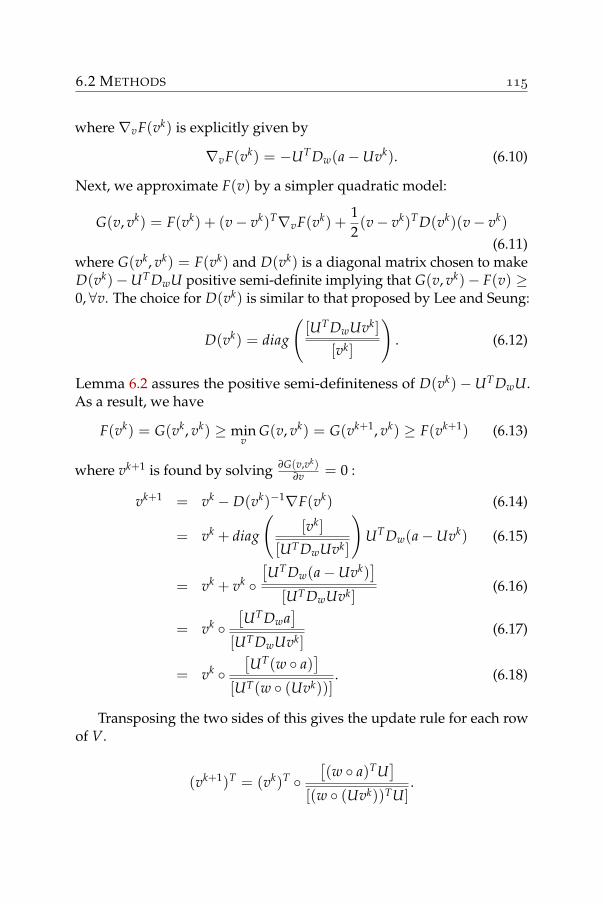
6.2 METHODS
where ∇vF(vk) is explicitly given by
∇vF(vk) = −UTDw(a−Uvk). (6.10)
Next, we approximate F(v) by a simpler quadratic model:
G(v, vk) = F(vk) + (v− vk)T∇vF(vk) +12(v− vk)TD(vk)(v− vk)
(6.11)where G(vk, vk) = F(vk) and D(vk) is a diagonal matrix chosen to makeD(vk)−UTDwU positive semi-definite implying that G(v, vk)− F(v) ≥0, ∀v. The choice for D(vk) is similar to that proposed by Lee and Seung:
D(vk) = diag
([UTDwUvk]
[vk]
). (6.12)
Lemma 6.2 assures the positive semi-definiteness of D(vk)−UTDwU.As a result, we have
F(vk) = G(vk, vk) ≥ minv
G(v, vk) = G(vk+1, vk) ≥ F(vk+1) (6.13)
where vk+1 is found by solving ∂G(v,vk)∂v = 0 :
vk+1 = vk − D(vk)−1∇F(vk) (6.14)
= vk + diag
([vk]
[UTDwUvk]
)UTDw(a−Uvk) (6.15)
= vk + vk [UTDw(a−Uvk)
][UTDwUvk]
(6.16)
= vk [UTDwa
][UTDwUvk]
(6.17)
= vk [UT(w a)
][UT(w (Uvk))]
. (6.18)
Transposing the two sides of this gives the update rule for each rowof V.
(vk+1)T = (vk)T [(w a)TU
][(w (Uvk))TU]
.
WEIGHTS IN NONNEGATIVE MATRIX FACTORIZATION
Putting together the updating rules for all the rows of V yieldsthe desired result for the whole matrix V in (6.6). The relation (6.13)shows that the weighted Euclidean distance is non-increasing underthe updating rule for V, and (6.14) show that vk+1 = vk if and onlyif vk ∇F(vk) = 0. Finally, the non-negativity of vk is automaticallysatisfied.
Similar to the original version of the multiplicative update rules,the above update rules suffer the same problem when approaching theboundary of the nonnegative orthant. When using this, one should startthe iteration from the interior of the nonnegative orthant and be cautiouswhen zeros appear in U and V.
6.2.2 Weighted Rank-one Residue Iteration
In Chapter 4, employing the rank partition of the NMF problem offersa simple coordinate descent algorithm for the NMF problem. Here,we will modify that algorithm to incorporate the weight matrix in thecost function. The Weighted Nonnegative Matrix Factorization can berestated as below:
Problem 6.4 (WNMF).
minui≥0 vi≥0
12‖A−
r
∑i=1
uivTi ‖2
W
where W is a nonnegative weight matrix.
To construct the update for vt, t = 1, 2, . . . , r, we fix all variablesexcept vt. Again, we create the residue matrix:
Rt = A−∑i 6=t
uivTi
to restrict Problem 6.4 only to the variable ut
minv≥0
12‖Rt − utvT‖2
W . (6.19)
6.2 METHODS
We have
‖Rt − utvT‖2W = ∑
ijWij([Rt]ij − [ut]ivj)2
= ∑ij
Wij
([Rt]2ij − 2[Rt]ij[ut]ivj + ([ut]ivj)2
)= ‖Rt‖2
W − 2 ∑j
vj
(∑
iWij[Rt]ij[ut]i
)
+ ∑j
v2j
(∑
iWiju2
i
)= ‖Rt‖2
W − 2vT(W Rt)Tut + (v v)TWT(ut ut).
From this formulation, one now can derive the following similarlemma to the one in Chapter 4.
Lemma 6.5. If [(W Rt)Tut]+ 6= 0 and WT(ut ut) > 0, then
v∗ :=[(W Rt)Tut]+
WT(ut ut)
is the unique global minimizer of (6.19) and the value of the cost function equals
12‖Rt−utv∗T‖2
W =12
‖Rt‖2W −
([(W Rt)Tut]+
WT(ut ut)
)T
[(W Rt)Tut]+
.
Proof. Let us permute the elements of the vectors x := (W Rt)Tut,y := WT(ut ut) and v such that
Px =(
x1x2
), Py =
(y1y2
)and Pv =
(v1v2
)with x1 ≥ 0, x2 < 0 and P is the permutation matrix. Then
‖Rt − utvT‖2W = ‖Rt‖2
W − 2vT1 x1 − 2vT
2 x2 + (vT1 Dy1 v1 + vT
2 Dy2 v2).
Since x2 < 0, v2 ≥ 0 and y > 0, it is obvious that ‖Rt − utvT‖2F can only
be minimal if v2 = 0. Our assumption implies that x+ is nonempty and
WEIGHTS IN NONNEGATIVE MATRIX FACTORIZATION
x1 ≥ 0. One can then find the optimal v1 by minimizing the remainingquadratic function
‖Rt‖2F − 2vT
1 x1 + vT1 Dy1 v1
which yields the solution v1 = [x1][y1]
. Putting the two components together
yields the result
v∗ =[x+][y]
and ‖Rt − utvT∗ ‖2
W = ‖Rt‖2W −
([x+][y]
)T
x+.
Remark 1: The above lemma has of course a dual form, where onefixes vt but solves for the optimal u to minimize ‖Rt − uvT
t ‖2W . These
lemmas would yield the updating rules
vt ←[(W Rt)Tut]+
WT(ut ut)and ut ←
[(W Rt)vt]+W(vt vt)
(6.20)
which can be used to recursively update approximations ∑ri=1 uivT
i bymodifying each rank-one matrix utvT
t in a cyclic manner. We call thismethod the Weighted Rank-one Residue Iteration (WRRI), which is shownin Algorithm 10.
Remark 2: In the case where [(W Rt)Tut]+ = 0, we have a trivialsolution for v = 0 that is not covered by Lemma 6.5. This solution isunique only when ut 6= 0. This will result in a rank-deficient approxima-tion. To avoid that, one can replace utvT
t by any rank-one approximationthat reduces the ‖.‖W norm of the error matrix, such as
u∗ = [(Rt W)i∗ :]+ v∗ = ei∗
where i∗ = argmaxi ‖[(Rt W)i:]+‖.Remark 3: If [WT(ut ut)]i = 0 for some i and because W ≥ 0 and
ut ≥ 0, one can conclude that [(W Rt)Tut]i = 0. This means that thecost function is unchanged irrespective of the value of v∗i . We can simplyset those elements of v∗ to zero to minimize ‖v∗‖2.
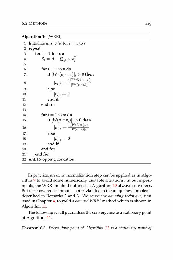
6.2 METHODS
Algorithm 10 (WRRI)
1: Initialize ui’s, vi’s, for i = 1 to r2: repeat3: for i = 1 to r do4: Ri = A−∑j 6=i ujvT
j5:6: for j = 1 to n do7: if [WT(ui ui)]j > 0 then
8: [vi]j ←([(WRi)Tui ]+)j
[WT(uiui)]j
9: else10: [vi]j ← 011: end if12: end for13:14: for j = 1 to m do15: if [W(vi vi)]j > 0 then
16: [ui]j ←([(WRi)vi ]+)j
[W(vivi)]j
17: else18: [ui]j ← 019: end if20: end for21: end for22: until Stopping condition
In practice, an extra normalization step can be applied as in Algo-rithm 9 to avoid some numerically unstable situations. In out experi-ments, the WRRI method outlined in Algorithm 10 always converges.But the convergence proof is not trivial due to the uniqueness problemsdescribed in Remarks 2 and 3. We reuse the damping technique, firstused in Chapter 4, to yield a damped WRRI method which is shown inAlgorithm 11.
The following result guarantees the convergence to a stationary pointof Algorithm 11.
Theorem 6.6. Every limit point of Algorithm 11 is a stationary point of
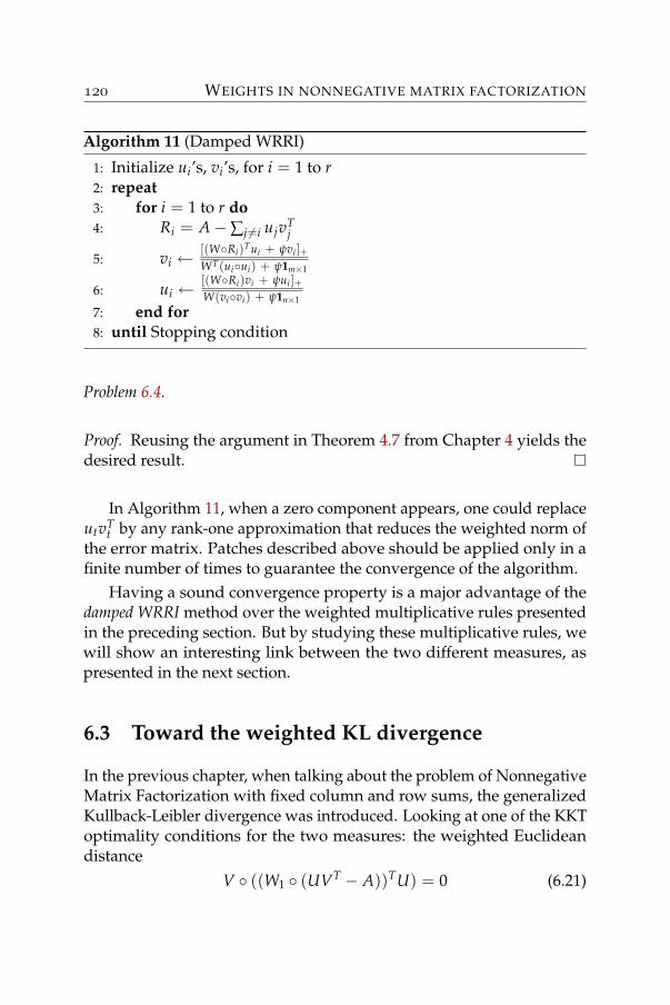
WEIGHTS IN NONNEGATIVE MATRIX FACTORIZATION
Algorithm 11 (Damped WRRI)
1: Initialize ui’s, vi’s, for i = 1 to r2: repeat3: for i = 1 to r do4: Ri = A−∑j 6=i ujvT
j
5: vi ←[(WRi)Tui + ψvi ]+WT(uiui) + ψ1m×1
6: ui ←[(WRi)vi + ψui ]+W(vivi) + ψ1n×1
7: end for8: until Stopping condition
Problem 6.4.
Proof. Reusing the argument in Theorem 4.7 from Chapter 4 yields thedesired result.
In Algorithm 11, when a zero component appears, one could replaceutvT
t by any rank-one approximation that reduces the weighted norm ofthe error matrix. Patches described above should be applied only in afinite number of times to guarantee the convergence of the algorithm.
Having a sound convergence property is a major advantage of thedamped WRRI method over the weighted multiplicative rules presentedin the preceding section. But by studying these multiplicative rules, wewill show an interesting link between the two different measures, aspresented in the next section.
6.3 Toward the weighted KL divergence
In the previous chapter, when talking about the problem of NonnegativeMatrix Factorization with fixed column and row sums, the generalizedKullback-Leibler divergence was introduced. Looking at one of the KKToptimality conditions for the two measures: the weighted Euclideandistance
V ((W1 (UVT − A))TU) = 0 (6.21)
6.3 TOWARD THE WEIGHTED KL DIVERGENCE
and the weighted KL divergence
V ((W2 (1m×n −[A]
[UVT]))TU) = 0, (6.22)
it is easy to see that if W1 = [W2][UVT ]
, these two conditions are identical,
where an additional assumption UVT > 0 has to be inserted. This meansthat, any stationary point given by an algorithm for weighted Euclideandistance is a stationary point of a corresponding weighted generalizedKL divergence. This can also be seen when extending the multiplicativeupdating rules [80] for the generalized KL divergence to the weightedcase. For the sake of completeness, we will include following theoremintroducing the multiplicative rules for the weighted generalized KLdivergence.
Theorem 6.7. The weighted divergence DW(A‖UV) is non-increasing underthe updating rules :
V ← [V][WTU]
([
WT AT][VUT]
U
), U ← [U]
[WV](
[W A][UVT]
V
).
(6.23)The weighted divergence DW(A‖UV) is invariant under these updates iff theconditions (5.5) and (5.7) hold.
Proof. Again, we prove the theorem only for V and we also split thedivergence into partial divergences corresponding to one column of Wand A, denoted by w and a.
F(v) = Dw(a‖Uv) (6.24)
= ∑i
wi
(ai log ai − ai + ∑
jUijvj − ai log ∑
jUijvj
),
where v is the transpose of the corresponding row of V. This partialdivergence is approximated by the following auxiliary function:
G(v, vk) = ∑i
(wi
(ai log ai − ai + ∑
jUijvj (6.25)
− ai ∑j
Uijvkj
∑l Uilvkl
(log Uijvj − log
Uijvkj
∑l Uilvkl
))).
WEIGHTS IN NONNEGATIVE MATRIX FACTORIZATION
Because of the convexity of the function−log(x) and since ∑jUijvk
j
∑l Uilvkl
= 1,
we have
− ai log ∑j
Uijvj = −ai log
(∑
j
Uijvkj
∑l UilvklUijvj
∑l Uilvkl
Uijvkj
)
≤ −ai ∑j
Uijvkj
∑l Uilvkl
log
(Uijvj
∑l Uilvkl
Uijvkj
)
≤ −ai ∑j
Uijvkj
∑l Uilvkl
(log Uijvj − log
Uijvkj
∑l Uilvkl
)
implying G(v, vk) ≥ F(v), ∀v. Moreover G(vk, vk) = F(vk), so weobtain:
F(vk) = G(vk, vk) ≥ minv
G(v, vk) = G(vk+1, vk) ≥ F(vk+1) . (6.26)
To obtain the updating rule, it is sufficient to construct the minimizer ofG with respect to v, given by:
∂G(v, vk)∂vj
= ∑i
wiUij −vk
j
vj∑
iwiai
Uij
∑l Uilvkl
= 0. (6.27)
Then the minimizer of G(v, vk) is chosen as the next value of v:
vk+1 =[vk]
[UTw](
UT [a w][Uvk]
). (6.28)
Transposing the two sides of this gives the update rule for each row ofV.
(vk+1)T =[(vk)T][wTU]
( [
aT wT][(vk)TUT]
U
). (6.29)
Putting together the updating rules for all the rows of V gives thedesired updating rule for the whole matrix V as in (6.23). The relation(6.26) shows that the weighted divergence is non increasing under theupdating rule for V. Using (6.29) and the fact that
∇F(vk) = UTw−UT [a w][Uvk]
(6.30)
6.3 TOWARD THE WEIGHTED KL DIVERGENCE
we can easily see that that vk+1 = vk if and only if vk ∇F(vk) = 0.Finally, the non-negativity of vk is automatically satisfied.
Having the updating rules for V for the weighted generalized KLdivergence, one can rewrite them as follows:
V ← [V][WTU]
([
WT AT][VUT]
U
)= V
[[WTAT]
[VUT ] U]
[ [WT(VUT)][VUT ] U
]
= V ( [
(WUVT A)TU]
[(WUVT (UVT))TU]
),
where WUVT = [W][UVT ]
. This shows that each update in the weighted
generalized KL divergence is equivalent to an update in the weightedEuclidean distance with the weight matrix WUVT . This is an adaptiveweighting since the weights change after each update. And at the station-ary point of this minimization, V and U converge to the minimizer ofthe weighted Euclidean distance for which the weight matrix is exactlyWUVT .
Conversely, one can see that each update in the weighted Euclideandistance with the weight matrix W is equivalent to an update in theweighted generalized KL divergence with the weight matrix WUVT =W (UVT). And again, at the stationary point of this minimization,U and V converge to the minimizer of the weighted generalized KLdivergence for which the weight matrix is exactly WUVT .
We summarize all the updating rules and the link between the twominimizations in Table 6.1. In the unweighted case, the matrix 1m×n isincluded to make it easier to compare it with the matrices W1 and W2of the weighted case. With our updating rules for the weighted case,we have thus shown that even though the two cost functions are verydifferent, their minimizations are closely related. While the convergenceof the multiplicative rules still needs further investigations, we canconclude this section by raising this question: which algorithms forweighted Euclidean distance (or weighted generalized KL divergence)converge to a stationary point when we add the adaptive weights as
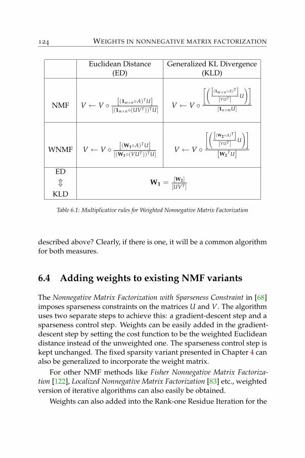
WEIGHTS IN NONNEGATIVE MATRIX FACTORIZATION
Euclidean Distance Generalized KL Divergence(ED) (KLD)
NMF V ← V [(1m×nA)TU][(1m×n(UVT))TU]
V ← V
[([(1m×nA)T]
[VUT ] U
)][1n×mU]
WNMF V ← V [(W1A)TU][(W1(VUT))TU]
V ← V
[([(W2A)T]
[VUT ] U
)][W2
TU]
EDm W1 = [W2]
[UVT ]KLD
Table 6.1: Multiplicative rules for Weighted Nonnegative Matrix Factorization
described above? Clearly, if there is one, it will be a common algorithmfor both measures.
6.4 Adding weights to existing NMF variants
The Nonnegative Matrix Factorization with Sparseness Constraint in [68]imposes sparseness constraints on the matrices U and V. The algorithmuses two separate steps to achieve this: a gradient-descent step and asparseness control step. Weights can be easily added in the gradient-descent step by setting the cost function to be the weighted Euclideandistance instead of the unweighted one. The sparseness control step iskept unchanged. The fixed sparsity variant presented in Chapter 4 canalso be generalized to incorporate the weight matrix.
For other NMF methods like Fisher Nonnegative Matrix Factoriza-tion [122], Localized Nonnegative Matrix Factorization [83] etc., weightedversion of iterative algorithms can also easily be obtained.
Weights can also added into the Rank-one Residue Iteration for the
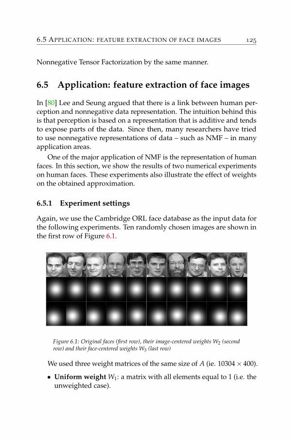
6.5 APPLICATION: FEATURE EXTRACTION OF FACE IMAGES
Nonnegative Tensor Factorization by the same manner.
6.5 Application: feature extraction of face images
In [80] Lee and Seung argued that there is a link between human per-ception and nonnegative data representation. The intuition behind thisis that perception is based on a representation that is additive and tendsto expose parts of the data. Since then, many researchers have triedto use nonnegative representations of data – such as NMF – in manyapplication areas.
One of the major application of NMF is the representation of humanfaces. In this section, we show the results of two numerical experimentson human faces. These experiments also illustrate the effect of weightson the obtained approximation.
6.5.1 Experiment settings
Again, we use the Cambridge ORL face database as the input data forthe following experiments. Ten randomly chosen images are shown inthe first row of Figure 6.1.
Figure 6.1: Original faces (first row), their image-centered weights W2 (secondrow) and their face-centered weights W3 (last row)
We used three weight matrices of the same size of A (ie. 10304× 400).
• Uniform weight W1: a matrix with all elements equal to 1 (i.e. theunweighted case).
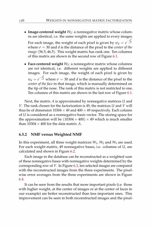
WEIGHTS IN NONNEGATIVE MATRIX FACTORIZATION
• Image-centered weight W2: a nonnegative matrix whose colum-ns are identical, i.e. the same weights are applied to every images.
For each image, the weight of each pixel is given by wd = e−d2
σ2
where σ = 30 and d is the distance of the pixel to the center of theimage (56.5, 46.5). This weight matrix has rank one. Ten columnsof this matrix are shown in the second row of Figure 6.1.
• Face-centered weight W3: a nonnegative matrix whose columnsare not identical, i.e. different weights are applied to differentimages. For each image, the weight of each pixel is given by
wd = e−d2
σ2 where σ = 30 and d is the distance of the pixel to thecenter of the face in that image, which is manually determined onthe tip of the nose. The rank of this matrix is not restricted to one.Ten columns of this matrix are shown in the last row of Figure 6.1.
Next, the matrix A is approximated by nonnegative matrices U andV. The rank chosen for the factorization is 49, the matrices U and V willthus be of dimension 10304× 49 and 400× 49 respectively. Each columnof U is considered as a nonnegative basis vector. The storing space forthe approximation will be (10304 + 400)× 49 which is much smallerthan 10304× 400 for the data matrix A.
6.5.2 NMF versus Weighted NMF
In this experiment, all three weight matrices W1, W2 and W3 are used.For each weight matrix, 49 nonnegative bases, i.e. columns of U, arecalculated and shown in Figure 6.2.
Each image in the database can be reconstructed as a weighted sumof these nonnegative bases with nonnegative weights determined by thecorresponding row of V. In Figure 6.3, ten selected images are comparedwith the reconstructed images from the three experiments. The pixel-wise error averages from the three experiments are shown in Figure6.4.
It can be seen from the results that more important pixels (i.e. thosewith higher weight, at the center of images or at the center of faces inour example) are better reconstructed than less important ones. Thisimprovement can be seen in both reconstructed images and the pixel-
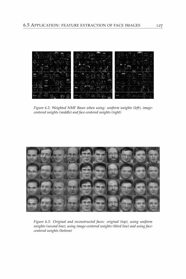
6.5 APPLICATION: FEATURE EXTRACTION OF FACE IMAGES
Figure 6.2: Weighted NMF Bases when using: uniform weights (left), image-centered weights (middle) and face-centered weights (right)
Figure 6.3: Original and reconstructed faces: original (top), using uniformweights (second line), using image-centered weights (third line) and using face-centered weights (bottom)
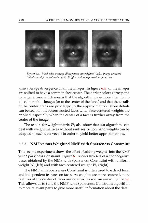
WEIGHTS IN NONNEGATIVE MATRIX FACTORIZATION
Figure 6.4: Pixel-wise average divergence: unweighted (left), image-centered(middle) and face-centered (right). Brighter colors represent larger errors.
wise average divergence of all the images. In figure 6.4, all the imagesare shifted to have a common face center. The darker colors correspondto larger errors, which means that the algorithm pays more attention tothe center of the images (or to the center of the faces) and that the detailsat the center areas are privileged in the approximation. More detailscan be seen on the reconstructed faces when face-centered weights areapplied, especially when the center of a face is further away from thecenter of the image.
The results for weight matrix W3 also show that our algorithms candeal with weight matrices without rank restriction. And weights can beadapted to each data vector in order to yield better approximations.
6.5.3 NMF versus Weighted NMF with Sparseness Constraint
This second experiment shows the effect of adding weights into the NMFwith Sparseness Constraint. Figure 6.5 shows two sets of 49 nonnegativebases obtained by the NMF with Sparseness Constraint with uniformweight W1 (left) and with face-centered weight W3 (right).
The NMF with Sparseness Constraint is often used to extract localand independent features on faces. As weights are more centered, morefeatures at the center of faces are retained as we can see in Figure 6.6.This allows us to tune the NMF with Sparseness Constraint algorithmto more relevant parts to give more useful information about the data.
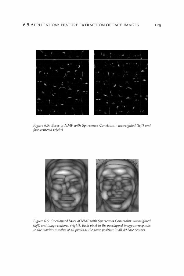
6.5 APPLICATION: FEATURE EXTRACTION OF FACE IMAGES
Figure 6.5: Bases of NMF with Sparseness Constraint: unweighted (left) andface-centered (right)
Figure 6.6: Overlapped bases of NMF with Sparseness Constraint: unweighted(left) and image-centered (right). Each pixel in the overlapped image correspondsto the maximum value of all pixels at the same position in all 49 base vectors.

WEIGHTS IN NONNEGATIVE MATRIX FACTORIZATION
7
SYMMETRY IN NONNEGATIVE MATRIXFACTORIZATION
Many data matrices are symmetric. This is the case for the adjacency ma-trix of an undirected graph, the matrix of geometric distances betweenpoints, correlation matrices, etc. We will investigate in this chapterthe symmetry constraint in the Nonnegative Matrix Factorization prob-lem. This leads to two new problems: Symmetric Nonnegative MatrixFactorization and Semi-Symmetric Nonnegative Matrix Factorization.
With the first problem, our objective is not only to obtain the sym-metry of the approximation but also a symmetric structure of the cor-responding factorization. While the NMF helps to find the UVT ap-proximation of a nonnegative matrix, its symmetric version tries to findapproximations where U = V. This allows us to link to other currentlyopen problems related to the completely positive matrices [10]. Since manyimportant questions about this topic are still very challenging, it is be-lieved that there is no efficient method for the problem SNMF. Until oneis found, we will try to solve the problem by looking for good approxi-mations rather than doing exhaustive search for the global optimum.
The second problem can be considered as a relaxed version of theSymmetric Nonnegative Matrix Factorization. As we will see, the addi-tional degrees of freedom in the Semi-Symmetric Nonnegative MatrixFactorization guarantees at least an exact approximation with finite in-ner rank of a arbitrary square nonnegative matrix, which is in generalimpossible with the Symmetric Nonnegative Matrix Factorization.
The chapter begins with a formal definition of the problem. Com-
SYMMETRY IN NONNEGATIVE MATRIX FACTORIZATION
pletely positive matrices are also discussed in the second part. Thena method to find good approximations is proposed. We mention someapplications of this special factorization including Graph Clustering andApproximation of Correlation Matrix.
7.1 Symmetric approximations
We will define two NMF problems in which some symmetries are im-posed on the factors. But first, we will discuss which structures of theapproximation are considered.
7.1.1 Symmetry of the approximation
As pointed out earlier, only the product of a factored approximation suchas those in the NMF problem can be considered as an approximation,since for a matrix B, there might be two different factorizations B =U1VT
1 and B = U2VT2 where (U1, V1) and (U2, V2) are different. The first
natural question to ask is: given a symmetric nonnegative matrix, whenwill the NMF approximation also be symmetric? This question is partiallyanswered in [25] through the two following theorems:
Theorem 7.1. Let A = QDQT be a non-negative symmetric matrix of rankt, t ≤ n, where Q ∈ Rn×n is orthogonal and D = diag(d1, ..., dt, 0..0),with di 6= −dj, for i, j ∈ 1, .., t, i 6= j. Let (U, V) be a solution to theNNMF problem (Euclidean Distance version) with∇U‖A−UVT‖2
F = 0 and∇V‖A−UVT‖2
F = 0. Then the product UV is (also) symmetric.
Theorem 7.2. Let A = QDQT be a non-negative symmetric matrix of rankt, t ≤ n, where Q ∈ Rn×n is orthogonal and D = diag(d1, ..., dt, 0..0),with di 6= dj, for i, j ∈ 1, .., t, i 6= j. Let (U, V) be a solution to theNNMF problem (Euclidean Distance version) with ∇U‖A −UVT‖2
F = 0and ∇V‖A−UVT‖2
F = 0. Assume rank(UV) = k ≤ t. Then the productUV is symmetric if and only if it is of the form UVT = QXQT where X =diag(x1, ..., xt, 0, ..., 0) with xi = 0 for all but k values of i1, ..., ik with xij =dij , j = 1, .., k.
These results are derived for NMF problem but only applied to thecases where∇U‖A−UVT‖2
F = 0 and∇V‖A−UVT‖2F = 0. This, in fact,
7.1 SYMMETRIC APPROXIMATIONS
targets only the unconstrained low-rank approximation problem andtherefore can be easily derived from Theorem 1.13 for both symmetricand non-symmetric matrices.
Notice that we can always construct a symmetric approximationof the same complexity (probably with higher rank) from a knownasymmetric approximation UVT. Indeed, taking
A =UVT + VUT
2
yields a symmetric approximation of A. Furthermore, it is a betterapproximation since∥∥∥∥A− UVT + VUT
2
∥∥∥∥ ≤ ‖A−UVT‖+ ‖A−UVT‖2
= ‖A−UVT‖
from the convexity of ‖.‖ and the symmetry of A.Because of that, we are interested in the problem where UVT is not
only symmetric but also U = V. In other words, we search for theUUT approximations where U is elementwise nonnegative. As we cansee in the following sections, this problem is more difficult to solvebut has more practical applications. A slightly different problem is toapproximate a square nonnegative matrix by the product USUT whereU and S are elementwise nonnegative [120]. With its special structure,the latter can be also applied to square non-symmetric matrices.
7.1.2 The problems
In this section, the two problems of interest are Symmetric NonnegativeMatrix Factorization and Semi-symmetric Nonnegative Matrix Factor-ization. The formal definition as well as some properties of these twoproblems will be presented in preparation for the section of methods.
Symmetric Nonnegative Matrix Factorization
The following problem is referred to as the Symmetric Nonnegative MatrixFactorization:
SYMMETRY IN NONNEGATIVE MATRIX FACTORIZATION
Problem 7.3 (SNMF).
minU∈Rn×r
+
12‖A−UUT‖2
F
where A is a n× n symmetric matrix and r is an integer.
As an usual optimization problem, we calculate the gradient of theobjective function on the factor U:
∇U12‖A−UUT‖2
F = UUTU − AU.
The KKT conditions are:
U ≥ 0 (7.1)UUTU − AU ≥ 0 (7.2)
U (UUTU − AU) = 0 (7.3)
It is known that the optimal nonnegative rank-one approximation isgiven by the Perron vectors. This remains true for the rank-one symmet-ric nonnegative factorization. But for the higher rank, the factorizationis no longer easy. This is, indeed, related to the well-known class ofcompletely positive matrices.
Every nonnegative matrix B that can be represented as UUT whereU is nonnegative is a completely positive (cp) matrix [10]. The aboveproblem is equivalent to find the nearest completely positive matrixwith rank r to the input matrix A. One important notion about thecp matrices is the completely positive rank (cp-rank) that is defined asthe minimum number of column of U such that B = UUT. We userank+
UUT (A) to denote the cp-rank of the matrix A. If A is not a cp matrix,we conventionally denote rank+
UUT (A) = +∞.The well-known problem of determining cp-rank of a symmetric
matrix A has been a subject many researches. Knowing a lower boundof this number, which is the ordinary rank of the matrix k = rank(A),the true general upper bound is still unknown. The best proved boundis k(k+1)
2 − 1 [7]. Two fundamental problems are:
• Deciding whether a matrix is a cp matrix.
7.1 SYMMETRIC APPROXIMATIONS
• Determining the cp-rank of a cp matrix.
They were open until recently, the application of Renegar algorithm[9] yields a finite method to compute the cp-rank of a matrix if it exists.But the complexity bound of this method is still non-polynomial. See[9] or Section 2.3 to derive this bound.
One of the necessary conditions for A symmetric to be completelypositive is that it must be positive semidefinite. When A is not, surely wecan not have an exact Symmetric Nonnegative Matrix Factorization forfinite rank. Knowing that the SNMF can not do better than the nearestsemidefinite positive matrix, the following results give a lower boundof the error function of SNMF approximation:
Theorem 7.4. Let A is be symmetric matrix. Then
minrank(B)=r
B0
‖A− B‖2F ≥ ∑
λi(A)<0(λi(A))2.
This is the simplified version of a theorem found in [57]. This resultimplies that when approximating a symmetric matrix by a semidefinitepositive matrix, one should only take into account the semidefinitepositive part A0 of the original matrix A. And applying the Eckart-Young theorem (Theorem 1.12) to the matrix A0 allows us to constructthe optimal approximation for the unconstrained problem.
A very simple example is the following matrix with its eigenvaluedecomposition:
A =
0 1 11 0 01 0 0
=√
2u1uT1 −√
2u2uT2 .
where u1 = (√
22
12
12 ) and u2 = (−
√2
212
12 ). Applying Theorem 7.4,
the best semidefinite positive approximation is the rank-one matrixA = A0 =
√2u1uT
1 . Observe that this approximation is also theoptimal SNMF approximation and therefore it is impossible to create abetter SNMF approximation even with higher ranks. This impossibilitycan be overcome if one uses a more flexible ’symmetric’ approximationintroduced by the second problem.
SYMMETRY IN NONNEGATIVE MATRIX FACTORIZATION
Semi-Symmetric Nonnegative Matrix Factorization
The following were first mentioned in [37, 120]. We refer to it as theSemi-Symmetric Nonnegative Matrix Factorization (SSNMF) problem:
Problem 7.5 (SSNMF).
minU∈Rn×r
+ S∈Rr×r‖A−USUT‖2
F
where A is a n× n nonnegative matrix and r is an integer.
For the symmetric matrix A, the matrix S is a way to absorb all thenonnegative eigenvalues. This is why the lower bound of the errorfor this type of approximation is exactly zero. The symmetry of Aalso allows us to assume further the symmetry of S. Since if S is notsymmetric, S∗ = S+ST
2 yields a better approximation∥∥∥∥A−U(
S + ST
2
)UT∥∥∥∥ ≤ ‖A−USUT‖+ ‖A−USTUT‖
2
= ‖A−USUT‖.
Consider again the above example. We have already seen that it isimpossible to create an exact UUT NMF approximation, but there existsan exact USUT approximation with r = 2:
A =
0 1 11 0 01 0 0
=
0 11 01 0
( 0 11 0
)(0 1 11 0 0
).
In fact, every nonnegative matrix admits at least one such exactapproximation (A = USUT) trivially given by U = I and S = A.And it is not limited to only symmetric nonnegative matrix but canbe also applied to an arbitrary square nonnegative matrix. We callthe minimum value of r that yields an exact approximation the Semi-Symmetric Nonnegative Rank denoted by rank+
USUT (A). Because it isbounded from above by n, the size of the original matrix, there is a finitealgorithm to compute this number using Renegar algorithm (crf. Section2.3).
The following result can be established to relate the different ranksof nonnegative factorizations presented in this thesis.
7.2 METHODS
Lemma 7.6. For every n× n square nonnegative matrix A, we have
rank(A) ≤ rank+UVT (A) ≤ rank+
USUT (A) ≤ n
andrank+
USUT (A) ≤ rank+UUT (A).
Proof. Trivial. Since the rank of every exact factorization of a rank− kmatrix can not have a smaller rank than k and we can create a UVT
factorization from USUT and USUT from UUT. The upper boundrank+
USUT (A) ≤ n is given by the trivial factorization U = I and S =A.
With the same argument used in the above Lemma, we can establish,in the following lemma, a similar relation of minimum error betweendifferent approximations of the same reduced rank r.
Lemma 7.7. For every n× n square nonnegative matrix A and r = 1, 2, . . .
minU,V∈Rn×r
‖A−UVT‖2F ≤ min
U,V∈Rn×r+
‖A−UVT‖2F
≤ minU∈Rn×r
+ S∈Rr×r‖A−USUT‖2
F
≤ minU∈Rn×r
+
‖A−UUT‖2F.
7.2 Methods
In this section, we provide some directions that one can follow to solvethe two above problems. Since it is not realistic to solve them optimally,we investigate some algorithms that can produce good approximationsfor the above problems.
7.2.1 Direct methods
Since the error function is differential, the gradient informations arealways available. Therefore, all gradient methods presented in Chapter3 can be reused for these problems.
SYMMETRY IN NONNEGATIVE MATRIX FACTORIZATION
7.2.2 Penalty methods
Our strategy is to guide the NMF algorithm to converge to a fixed pointof SNMF if possible. We start the NNMF algorithm with an asymmetricstarting point (i.e. U0VT
0 ), and then force the two factors (i.e. Uk and Vk)to be equal by minimizing their normed difference. One way to do is touse the following modified cost function for a symmetric matrix A:
Fs(A, UVT) =12‖A−UVT‖2
F +α
2‖U −V‖2
F, α > 0 (7.4)
where the earlier part ( 12‖A−UVT‖2
F) is called the approximationerror and the latter part ( 1
2‖U −V‖2F) is called the asymmetry penalty.
We will derive two methods based on the Multiplicative Rules andthe Rank-one Residue Iteration scheme for solving the following prob-lem:
Problem 7.8.min
U∈Rn×r+ V∈Rn×r
+
Fs(A, UVT).
Regularized multiplicative rules
Incorporating additional linear or quadratic costs with the EuclideanDistance does not change significantly the updating rules. Using thesame reasoning for constructing the multiplicative updating rules, onecan obtain Algorithm 12 for the SNMF problem.
Different from the original algorithm, the regularized version needsthe following balancing step after each update of U (step 4) or V (step5). These consist in balancing the norm of each column of U and that ofthe corresponding column of V
Dii =√‖V:,i‖√‖U:,i‖
U = UD V = VD−1. (7.5)
Regularized rank-one residue iteration
We modify the algorithm presented in Chapter 4 by taking into accountthe regularized cost function. The elementary Rank-one problem be-
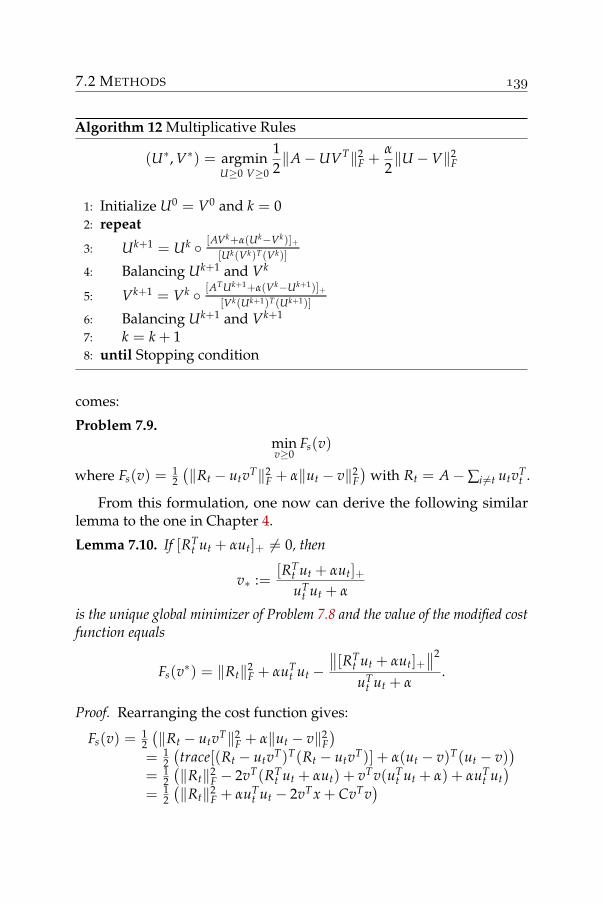
7.2 METHODS
Algorithm 12 Multiplicative Rules
(U∗, V∗) = argminU≥0 V≥0
12‖A−UVT‖2
F +α
2‖U −V‖2
F
1: Initialize U0 = V0 and k = 02: repeat
3: Uk+1 = Uk [AVk+α(Uk−Vk)]+[Uk(Vk)T(Vk)]
4: Balancing Uk+1 and Vk
5: Vk+1 = Vk [ATUk+1+α(Vk−Uk+1)]+[Vk(Uk+1)T(Uk+1)]
6: Balancing Uk+1 and Vk+1
7: k = k + 18: until Stopping condition
comes:
Problem 7.9.minv≥0
Fs(v)
where Fs(v) = 12
(‖Rt − utvT‖2
F + α‖ut − v‖2F)
with Rt = A−∑i 6=t utvTt .
From this formulation, one now can derive the following similarlemma to the one in Chapter 4.
Lemma 7.10. If [RTt ut + αut]+ 6= 0, then
v∗ :=[RT
t ut + αut]+uT
t ut + α
is the unique global minimizer of Problem 7.8 and the value of the modified costfunction equals
Fs(v∗) = ‖Rt‖2F + αuT
t ut −∥∥[RT
t ut + αut]+∥∥2
uTt ut + α
.
Proof. Rearranging the cost function gives:
Fs(v) = 12
(‖Rt − utvT‖2
F + α‖ut − v‖2F)
= 12
(trace[(Rt − utvT)T(Rt − utvT)] + α(ut − v)T(ut − v)
)= 1
2
(‖Rt‖2
F − 2vT(RTt ut + αut) + vTv(uT
t ut + α) + αuTt ut)
= 12
(‖Rt‖2
F + αuTt ut − 2vTx + CvTv
)
SYMMETRY IN NONNEGATIVE MATRIX FACTORIZATION
where x := RTt ut + αut and C := uT
t ut + α.Let us permute the elements of the vectors x and v such that
Px =(
x1x2
)and Pv =
(v1v2
)with x1 ≥ 0, x2 < 0 and P is the permutation matrix. Then
Fs(v) = ‖Rt‖2 + αuTt ut − 2vT
1 x1 − 2vT2 x2 + C(vT
1 v1 + vT2 v2).
Since x2 < 0, v2 ≥ 0 and C ≥ 0, it is obvious that the modified costfunction can only be minimal if v2 = 0. Our assumption implies that x+is nonempty and x1 ≥ 0. One can then find the optimal v1 by minimizingthe remaining quadratic function
‖Rt‖2F + αuT
t ut − 2vT1 x1 + CvT
1 v1
which yields the solution v1 = x1C . Putting the two components together
yields the result
v∗ =x+
Cand Fs(v∗) = ‖Rt‖2
F + αuTt ut −
‖x+‖2
C.
In the case where [RTt ut + αut]+ = 0, we have a unique optimal
solution: v∗ = 0 that is not covered by Lemma 7.10. This solution isunique even when ut = 0. But this will result in a zero component inthe approximation.
An update for ut can be similarly formulated. Using these to iteratethrough all the ui’s and vi’s yields Algorithm 13 for the modified costfunction.
In Algorithm 13, balancing steps (7) and (11) are added after eachupdate. This does not increase the approximation error ‖A−UVT‖2
Fbut decreases the asymmetry penalty ‖U − V‖2
F, hence yields a morebalanced factorization that helps the algorithm to converge to the sym-metric fixed point. This is also a way to restrict all variables inside somecompact sets and it is hence easy to show that every limit point is astationary point.
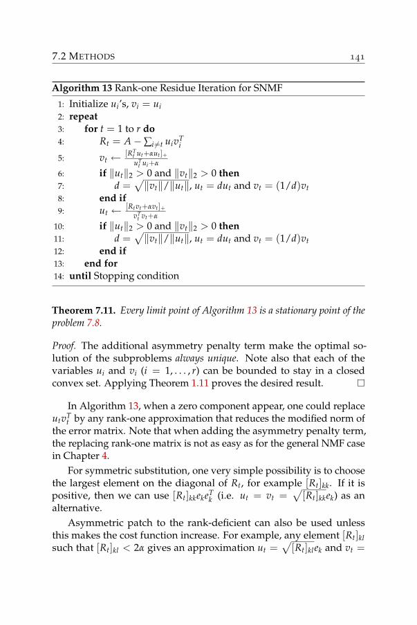
7.2 METHODS
Algorithm 13 Rank-one Residue Iteration for SNMF
1: Initialize ui’s, vi = ui2: repeat3: for t = 1 to r do4: Rt = A−∑i 6=t uivT
i
5: vt ← [RTt ut+αut]+uT
t ui+α
6: if ‖ut‖2 > 0 and ‖vt‖2 > 0 then7: d =
√‖vt‖/‖ut‖, ut = dut and vt = (1/d)vt
8: end if9: ut ← [Rtvt+αvt]+
vTt vt+α
10: if ‖ut‖2 > 0 and ‖vt‖2 > 0 then11: d =
√‖vt‖/‖ut‖, ut = dut and vt = (1/d)vt
12: end if13: end for14: until Stopping condition
Theorem 7.11. Every limit point of Algorithm 13 is a stationary point of theproblem 7.8.
Proof. The additional asymmetry penalty term make the optimal so-lution of the subproblems always unique. Note also that each of thevariables ui and vi (i = 1, . . . , r) can be bounded to stay in a closedconvex set. Applying Theorem 1.11 proves the desired result.
In Algorithm 13, when a zero component appear, one could replaceutvT
t by any rank-one approximation that reduces the modified norm ofthe error matrix. Note that when adding the asymmetry penalty term,the replacing rank-one matrix is not as easy as for the general NMF casein Chapter 4.
For symmetric substitution, one very simple possibility is to choosethe largest element on the diagonal of Rt, for example [Rt]kk. If it ispositive, then we can use [Rt]kkekeT
k (i.e. ut = vt =√
[Rt]kkek) as analternative.
Asymmetric patch to the rank-deficient can also be used unlessthis makes the cost function increase. For example, any element [Rt]klsuch that [Rt]kl < 2α gives an approximation ut =
√[Rt]klek and vt =
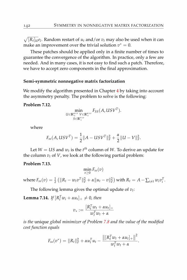
SYMMETRY IN NONNEGATIVE MATRIX FACTORIZATION
√[Rt]klel . Random restart of ut and/or vt may also be used when it can
make an improvement over the trivial solution v∗ = 0.These patches should be applied only in a finite number of times to
guarantee the convergence of the algorithm. In practice, only a few areneeded. And in many cases, it is not easy to find such a patch. Therefore,we have to accept zero components in the final approximation.
Semi-symmetric nonnegative matrix factorization
We modify the algorithm presented in Chapter 4 by taking into accountthe asymmetry penalty. The problem to solve is the following:
Problem 7.12.min
U∈Rn×r+ V∈Rn×r
+S∈Rr×r
+
FSS(A, USVT).
where
Fss(A, USVT) =12‖A−USVT‖2
F +α
2‖U −V‖2
F.
Let W = US and wt is the tth column of W. To derive an update forthe column vt of V, we look at the following partial problem:
Problem 7.13.minv≥0
Fss(v)
where Fss(v) = 12
(‖Rt − wtvT‖2
F + α‖ut − v‖2F)
with Rt = A−∑i 6=t wivTi .
The following lemma gives the optimal update of vt:
Lemma 7.14. If [RTt wi + αut]+ 6= 0, then
v∗ :=[RT
t wt + αut]+wT
t wt + α
is the unique global minimizer of Problem 7.8 and the value of the modifiedcost function equals
Fss(v∗) = ‖Rt‖2F + αuT
t ut −∥∥[RT
t wt + αut]+∥∥2
wTt wt + α
.
7.2 METHODS
Remark: when [RTt wt + αut]+ = 0, which is not covered by Lemma
7.14, the unique optimal update is v∗ = 0, even when ut = 0.The proof of this lemma is similar to Lemma 7.10 and is skipped. A
similar development yields the update for ut:
u∗ :=[Qtyt + αvt]+
yTt yt + α
where yt is the tth column of Y = VST and Qt = A−∑i 6=t uiyTi .
Now, we need to update S given U and V. We choose to update eachelement of S separately. We can rewrite the approximation error as:
‖A−USVT‖2F = ‖A−∑
ijSijuivT
j ‖2F
= ‖(A− ∑(i,j) 6=(k,l)
SijuivTj )− SklukvT
l ‖2F
= ‖Pkl − SklukvTl ‖2
F
where Pkl is the residue matrix A − ∑(i,j) 6=(k,l) SijuivTj . This is a very
simple scaling problem. But the optimal solution is only unique if‖uk‖2 > 0 and ‖vl‖ > 0:
S∗kl = max
(uT
k Pklvl
uTk ukvT
l vl, 0
).
Since the uniqueness is needed for the convergence, therefore, one canagain use the damping method described in Section 4.3 for the variableS. This is done by introducing a dummy variable T and a small positiveconstant ψ and adding the terms ψ
2 ‖S− T‖2F to the cost function. Using
the same development in Section 4.3, we have the following update forSkl :
S∗kl = max
(uT
k Pklvl + ψSkl
uTk ukvT
l vl + ψ, 0
).
Putting all together yields Algorithm 14.The normalization step (18) in Algorithm 14 consists of finding two
positive diagonal matrix DU and DV and updating:
U = UDU , V = VDV and S = D−1U SD−1
V ,
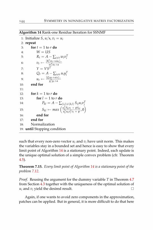
SYMMETRY IN NONNEGATIVE MATRIX FACTORIZATION
Algorithm 14 Rank-one Residue Iteration for SSNMF
1: Initialize S, ui’s, vi = ui2: repeat3: for t = 1 to r do4: W = US5: Rt = A−∑i 6=t wivT
i
6: vt ← [RTt wt+αut]+wT
t wt+α
7: Y = VST
8: Qt = A−∑i 6=t uiyTi
9: ut ← [Qtyt+αvt]+yT
t yt+α
10: end for11:12: for k = 1 to r do13: for l = 1 to r do14: Pkl = A−∑(i,j) 6=(k,l) SijuivT
j
15: Skl ← max(
uTk Pklvl + ψSkl
uTk ukvT
l vl + ψ, 0)
16: end for17: end for18: Normalization19: until Stopping condition
such that every non-zero vector ui and vi have unit norm. This makesthe variables stay in a bounded set and hence is easy to show that everylimit point of Algorithm 14 is a stationary point. Indeed, each update isthe unique optimal solution of a simple convex problem (cfr. Theorem4.5).
Theorem 7.15. Every limit point of Algorithm 14 is a stationary point of theproblem 7.12.
Proof. Reusing the argument for the dummy variable T in Theorem 4.7from Section 4.3 together with the uniqueness of the optimal solution ofui and vi yield the desired result.
Again, if one wants to avoid zero components in the approximation,patches can be applied. But in general, it is more difficult to do that here
7.2 METHODS
than in the previous section. But one can always take a random vectorfor the corresponding column of S. It must be done with care becausethis may increase the cost function. If we can not find an acceptable fix,then we should accept the solution v∗ = 0 and wait for the next sweep.If found, the patches should be applied in only a finite number of timesto guarantee the convergence of the algorithm.
Regularizing constant
The parameter α appears in the two previous formulations as the trade-off between the approximation error and the asymmetry penalty ofthe fixed point. The right choices of α can lead the search directiontoward the symmetric fixed points. Overestimating α could lead to asymmetric factorization without taking into account the approximationerror. And α = 0 means that the penalty is absent, hence becomes theNMF Algorithm 7.
An appropriate value of α is believed to depend on the best possibleapproximation error, but this error is not known in general. Experimentsshow that the range of possible values of α is quite large, so that, onecan restart the algorithm with a better value of α determined from theprevious results of the algorithm.
It is also useful to note that, after all, the results might not be in thedesired form in which U = V. But by having forced the symmetry, onecan expect that the errors ‖A −UUT‖2
F (or ‖A −USUT‖2F) and ‖A −
VVT‖2F (or ‖A−VSVT‖2
F) are not too far from the real approximationerror ‖A−UVT‖2
F (or ‖A−UVT‖2F). One could even used U∗ = U+V
2as a solution.
In practice, the symmetry regularization does not only force the fac-tors to be equal, but it can also lead to a better approximation. There areexamples where the symmetric approximation is better than the asym-metric one. But applying the general algorithms for NMF problem mayhave difficulty to converge to a symmetric approximation. An exampleis when we applied NMF method to the well-known iris flower data[43]. It consists of a 150× 4 matrix X whose rows contain 4 measuresof a flower: the sepal length, the sepal width, the petal length and thepetal width. There are 3 species in the dataset (1− 50: setosa, 51− 100:versicolor and 101− 150: virginica). We construct the similarity matrix
SYMMETRY IN NONNEGATIVE MATRIX FACTORIZATION
between the flowers S = XXT. We apply Algorithm 13 to the similaritymatrix S with three different values of α = 0, 1 and 50 and with thereduced rank r = 3. Note again that, α = 0 removes the penalty from thecost function. We present here the plot of 4 functions for each iterationof the Rank-one Residue Iteration algorithm:
• the full cost function: f α1 (Uk, Vk) = 1
2‖A−UkVTk ‖2
F + α2‖Uk−Vk‖2
F,
• the asymmetry error: f2(Uk, Vk) = 12‖Uk −Vk‖2
F,
• the approximation error of UVT: f3(Uk, Vk) = ‖A−UUT‖2F
• the approximation error of UUT: f4(Uk) = ‖A−UUT‖2F
• and the approximation error of VVT: f5(Vk) = ‖A−VVT‖2F.
Figure 7.1: Full cost function for different values of α
Figure 7.1 shows that the asymmetric algorithm (α = 0) can not convergeto the lower error approximation. It was trapped in an asymmetric localminimum, which yields a large approximation error. The asymmetryerror function ( f2) shows that the approximation is totally not symmetric.
7.2 METHODS
Figure 7.2: Asymmetry error for different values of α
Figure 7.3: Approximation error of UVT for different values of α
SYMMETRY IN NONNEGATIVE MATRIX FACTORIZATION
Figure 7.4: Approximation error of UUT for different values of α
Figure 7.5: Approximation error of VVT for different values of α

7.2 METHODS
The approximation errors produced by UUT and VVT stay high. Forα = 1, there is an improvement in all measures. But the convergenceis still very slow. When we increase α to 50, Algorithm 13 produces asymmetric approximation with a lower error than the asymmetric one.Furthermore, it converges much faster. In fact, in this example, it is verylikely that the best approximation is symmetric (i.e. UUT) because theinput matrix S is cp by construction.
In general, when approximating a matrix, if we know that the bestapproximation is symmetric, we can add the described regularization toguide the algorithm eventually to the global minimizer. In this case, thesymmetry plays a role of prior knowledge of the problem that one canprovide to the algorithm.
For the Semi-Symmetric Nonnegative Matrix Factorization, we ob-served the same phenomena.
Sparse approximation
The factor U in the two symmetric problems plays a central role in theirclustering applications where the sparsity of U is required. We can there-fore modify the above algorithms to create sparser approximation. Asimple technique is to add extra regularization term β(∑i ‖ui‖1 + ‖vi‖1)to the cost function (7.4), as suggested in [21]. This will slightly modifythe update for U and V but a sparser approximation can be obtained.
The modified updates are:
• Symmetric Nonnegative Matrix Factorization:
vt ←[RT
t ut + αut − β1n×1]+uT
t ut + αand ut ←
[Rtvt + αvt − β1n×1]+vT
t vt + α.
• Semi-Symmetric Nonnegative Matrix Factorization:
vt ←[RT
t wt + αut − β1n×1]+wT
t wt + αand ut ←
[Qtyt + αvt − β1n×1]+yT
t yt + α.
SYMMETRY IN NONNEGATIVE MATRIX FACTORIZATION
7.3 Applications: graph clustering
Clustering is one of the central problems in data analysis and exploration.Clustering amounts to finding out the structure of data by dividingelements into groups while maximizing the similarity or the connectivitybetween elements in the same group and at the same time, minimizingthese quantities between elements that are not in the same group.
The graph clustering is a particular case where vertices of a graph arepartitioned into different group so that inside each group, the connec-tivity or similarity [18] is high, while the connectivity or the similaritybetween different groups is low. We will see how the problem of a graphclustering based on the connectivity of graph can be reformulated as aproblem of Symmetric Nonnegative Matrix Factorization.
In general, one can define the graph clustering problem as follows:Given an integer k > 0 and a graph G = (V, E), where V (|V| = n) is the setof vertices and E is the set of edges, find a partition of V: C = C1, ..., Ck thatmaximizes a specified performance function f (G, C).
In this definition, each of the sets Ci is a cluster and C is called aclustering.
For the connectivity case, the input graph is usually undirected ormade to be undirected, implying that if vertex i is connected to vertex j(i.e. (i, j) ∈ E), then vertex j is also connected to vertex i (i.e. (j, i) ∈ E).We further assume that each vertex of the graph is connected to itself(i.e. (i, i) ∈ E).
The choice of f depends on each application and it will determinethe nature of the clusters. For the connectivity case, we use the followingconnectivity performance function [22]:
cper f (G, C) =# (i, j) ∈ E| (i, j) ∈ C + # (i, j) /∈ E| (i, j) /∈ C
n2 ,(7.6)
where (i, j) ∈ C means that i and j belong to the same cluster in C orin other words, the edge (i, j) is in the clustering C. The first value in thenumerator # (i, j) ∈ E|(i, j) ∈ C is the number of edges which are incommon to E and the clustering C. And the second value is the numberof edges which are not common to E and C. We see that the numerator
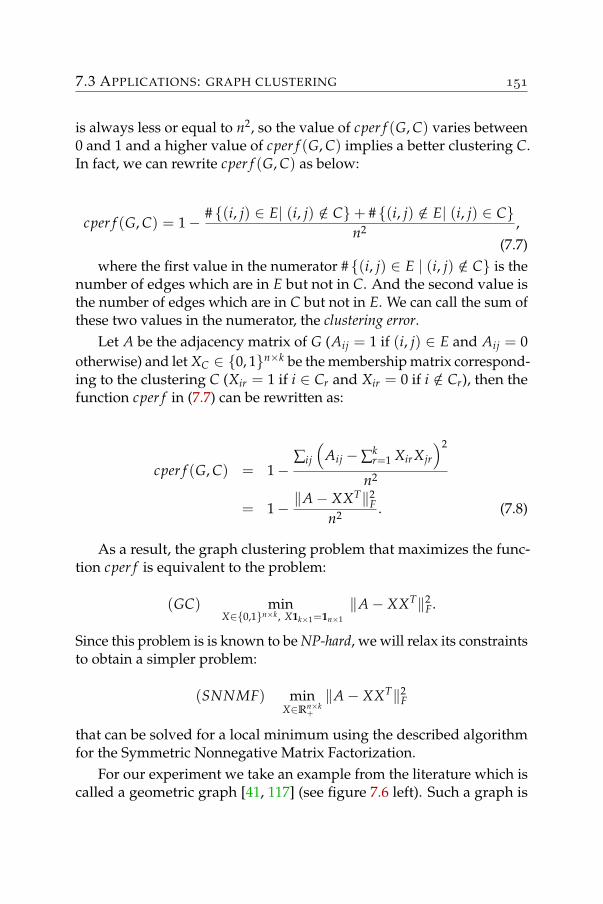
7.3 APPLICATIONS: GRAPH CLUSTERING
is always less or equal to n2, so the value of cper f (G, C) varies between0 and 1 and a higher value of cper f (G, C) implies a better clustering C.In fact, we can rewrite cper f (G, C) as below:
cper f (G, C) = 1− # (i, j) ∈ E| (i, j) /∈ C+ # (i, j) /∈ E| (i, j) ∈ Cn2 ,
(7.7)where the first value in the numerator # (i, j) ∈ E | (i, j) /∈ C is the
number of edges which are in E but not in C. And the second value isthe number of edges which are in C but not in E. We can call the sum ofthese two values in the numerator, the clustering error.
Let A be the adjacency matrix of G (Aij = 1 if (i, j) ∈ E and Aij = 0otherwise) and let XC ∈ 0, 1n×k be the membership matrix correspond-ing to the clustering C (Xir = 1 if i ∈ Cr and Xir = 0 if i /∈ Cr), then thefunction cper f in (7.7) can be rewritten as:
cper f (G, C) = 1−∑ij
(Aij −∑k
r=1 XirXjr
)2
n2
= 1− ‖A− XXT‖2F
n2 . (7.8)
As a result, the graph clustering problem that maximizes the func-tion cper f is equivalent to the problem:
(GC) minX∈0,1n×k , X1k×1=1n×1
‖A− XXT‖2F.
Since this problem is is known to be NP-hard, we will relax its constraintsto obtain a simpler problem:
(SNNMF) minX∈Rn×k
+
‖A− XXT‖2F
that can be solved for a local minimum using the described algorithmfor the Symmetric Nonnegative Matrix Factorization.
For our experiment we take an example from the literature which iscalled a geometric graph [41, 117] (see figure 7.6 left). Such a graph is
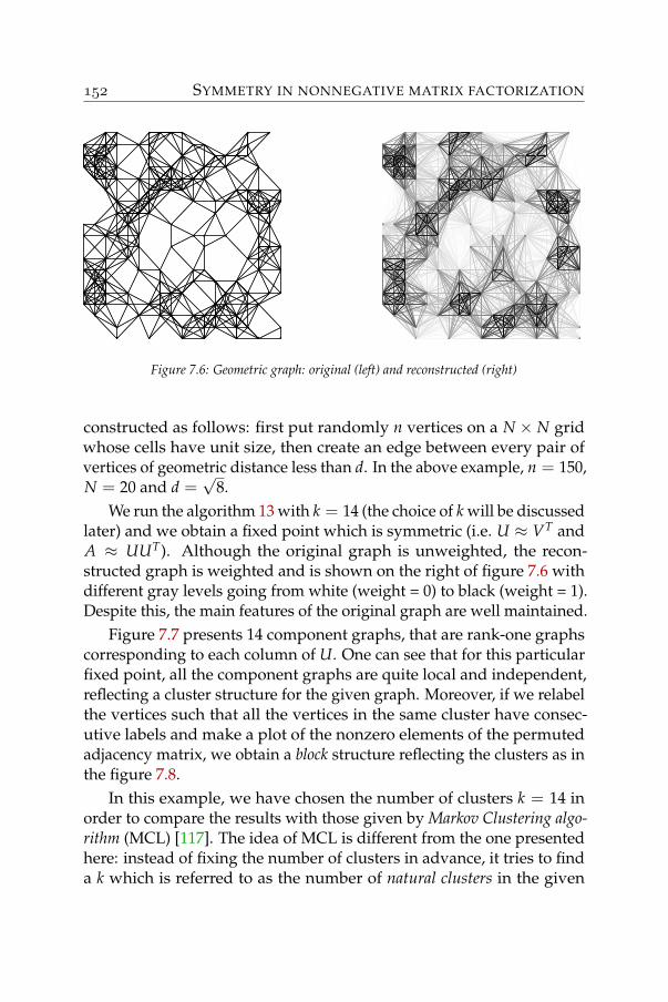
SYMMETRY IN NONNEGATIVE MATRIX FACTORIZATION
Figure 7.6: Geometric graph: original (left) and reconstructed (right)
constructed as follows: first put randomly n vertices on a N × N gridwhose cells have unit size, then create an edge between every pair ofvertices of geometric distance less than d. In the above example, n = 150,N = 20 and d =
√8.
We run the algorithm 13 with k = 14 (the choice of k will be discussedlater) and we obtain a fixed point which is symmetric (i.e. U ≈ VT andA ≈ UUT). Although the original graph is unweighted, the recon-structed graph is weighted and is shown on the right of figure 7.6 withdifferent gray levels going from white (weight = 0) to black (weight = 1).Despite this, the main features of the original graph are well maintained.
Figure 7.7 presents 14 component graphs, that are rank-one graphscorresponding to each column of U. One can see that for this particularfixed point, all the component graphs are quite local and independent,reflecting a cluster structure for the given graph. Moreover, if we relabelthe vertices such that all the vertices in the same cluster have consec-utive labels and make a plot of the nonzero elements of the permutedadjacency matrix, we obtain a block structure reflecting the clusters as inthe figure 7.8.
In this example, we have chosen the number of clusters k = 14 inorder to compare the results with those given by Markov Clustering algo-rithm (MCL) [117]. The idea of MCL is different from the one presentedhere: instead of fixing the number of clusters in advance, it tries to finda k which is referred to as the number of natural clusters in the given
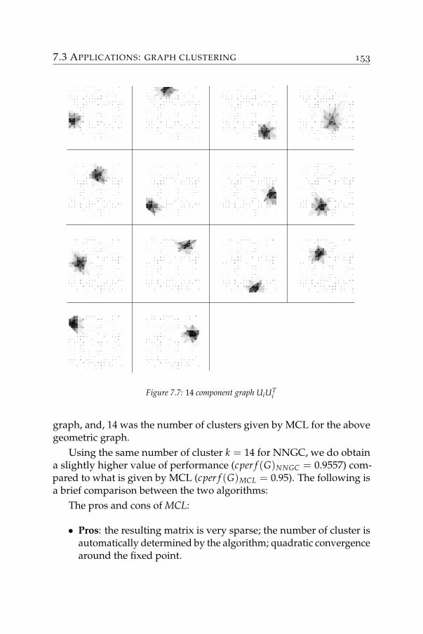
7.3 APPLICATIONS: GRAPH CLUSTERING
Figure 7.7: 14 component graph UiUTi
graph, and, 14 was the number of clusters given by MCL for the abovegeometric graph.
Using the same number of cluster k = 14 for NNGC, we do obtaina slightly higher value of performance (cper f (G)NNGC = 0.9557) com-pared to what is given by MCL (cper f (G)MCL = 0.95). The following isa brief comparison between the two algorithms:
The pros and cons of MCL:
• Pros: the resulting matrix is very sparse; the number of cluster isautomatically determined by the algorithm; quadratic convergencearound the fixed point.
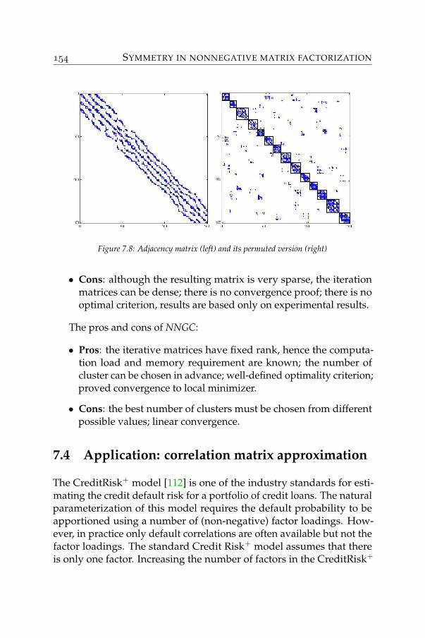
SYMMETRY IN NONNEGATIVE MATRIX FACTORIZATION
Figure 7.8: Adjacency matrix (left) and its permuted version (right)
• Cons: although the resulting matrix is very sparse, the iterationmatrices can be dense; there is no convergence proof; there is nooptimal criterion, results are based only on experimental results.
The pros and cons of NNGC:
• Pros: the iterative matrices have fixed rank, hence the computa-tion load and memory requirement are known; the number ofcluster can be chosen in advance; well-defined optimality criterion;proved convergence to local minimizer.
• Cons: the best number of clusters must be chosen from differentpossible values; linear convergence.
7.4 Application: correlation matrix approximation
The CreditRisk+ model [112] is one of the industry standards for esti-mating the credit default risk for a portfolio of credit loans. The naturalparameterization of this model requires the default probability to beapportioned using a number of (non-negative) factor loadings. How-ever, in practice only default correlations are often available but not thefactor loadings. The standard Credit Risk+ model assumes that thereis only one factor. Increasing the number of factors in the CreditRisk+
7.4 APPLICATION: CORRELATION MATRIX APPROXIMATION
model is always tied to increasing the rank of the approximation forthe default correlation matrix. Ultimately, the use of as many factorsas credit exposures would allow to reproduce the correlation matrixexactly. In principle, this would lead to the most accurate approxima-tion. The following is a summary of the application of the SymmetricNonnegative Matrix Factorization to the CreditRisk+ model. For moredetails, the interested reader is referred to [119].
In this context, the “Credit Portfolio Loss” is modeled by the follow-ing random variable S, :
S =n
∑i=1
Ni ci, (7.9)
where we assume that ci’s are known. The multivariate distribution ofN =
[N1 N2 . . . Nn
]T is defined with the assumption that there
exists a random vector Γ =[
Γ1 . . . ΓK]Trepresenting the “state of
the economy” such that the random variables Ni, conditioned by Γk =γk, (k = 1, 2, ..., K), are mutually independent and Poisson distributedwith intensity:
Ri = qi
(w0,i +
K
∑k=1
wk,iγk
), (7.10)
where qi is the probability that the risk i leads to a failure.The coefficient w0,i reflects the portion of idiosyncratic risk that can
be attributed to the i-th risk whereas wk,i reflects its affiliation to the k-thcommon factor. It is important to note that in order to have positiveintensities in (7.10), the coefficients wk,i , k = 0, 1, ..., K will be constrainedto be non-negative.
The random variables Γi are assumed to be independent Gammadistributed and the covariance matrix associated with the random vectorΓ is given by:
cov[Γ] = Σ :=
σ21
. . .σ2
K
.
Since the random variable aΓk will be distributed like a Gamma randomvariable for any k and a > 0, we can assume without loss of generalitythat E[Γi] = 1.
SYMMETRY IN NONNEGATIVE MATRIX FACTORIZATION
The modeled covariance matrix covM[N] associated with the randomvector N is then calculated as:
covM[N] = QWTΣWQ + Q (7.11)
where Q = diag(q1, q2, . . . , qn) and W = wikm,ki=1, k=1
On the other hand, we can calculate the covariance matrix from theknown default correlation matrix C:
covR[N] = [Q(I −Q)]1/2C[Q(I −Q)]1/2 + Q.
Equating the two covariance matrices covM[N] = covR[N], we have:
QWTΣWQ = [Q(I −Q)]1/2C[Q(I −Q)]1/2. (7.12)
Note again that, the matrix W ≥ 0 contains the parameter matrixof the model that need to be found. From the relation (7.12), one cantherefore approximating the matrix Q−1/2(I −Q)1/2C(I −Q)1/2Q−1/2
by using one of the Symmetric Nonnegative Matrix Factorization algo-rithms, for example RRISNMF (Algorithm 13). To have the matrices Wand Σ from the resulted approximation UUT, one needs only to choosethe appropriate positive weight matrix Σ and compute W = UΣ−1/2.
In [119], we carried out this idea to the real data matrix taken fromthe default correlation data between clients of a Belgian bank. Becauseit has millions of clients and the correlation matrix is in general notsparse, the corresponding correlation matrix will be very large evenfor storing, if we take into account all the clients. One preprocessingstep is performed to divide its clients into clusters and to compute onlythe correlation information between these clusters. The current versionof this clustered correlation matrix has dimension 1513 which is quitereasonable. All experiments in this section are carried out on this matrix.
In order to obtain a low-rank non-negative approximation of thecorrelation matrix, the RRISNMF algorithm and the symmetric mul-tiplicative rules (SMULT) have been used for increasing values of thenumber of factor K of systematic risks. This number K is also equalto the rank of the non-negative factorization of C. Figure 7.9, 7.10 and7.11 present the behavior of both algorithms (RRISNMF and SMULT) incalculating low-rank approximations (rank = 5, 20 and 50) of the correla-tion matrix. It is easy to see that the RRISNMF algorithm converges in
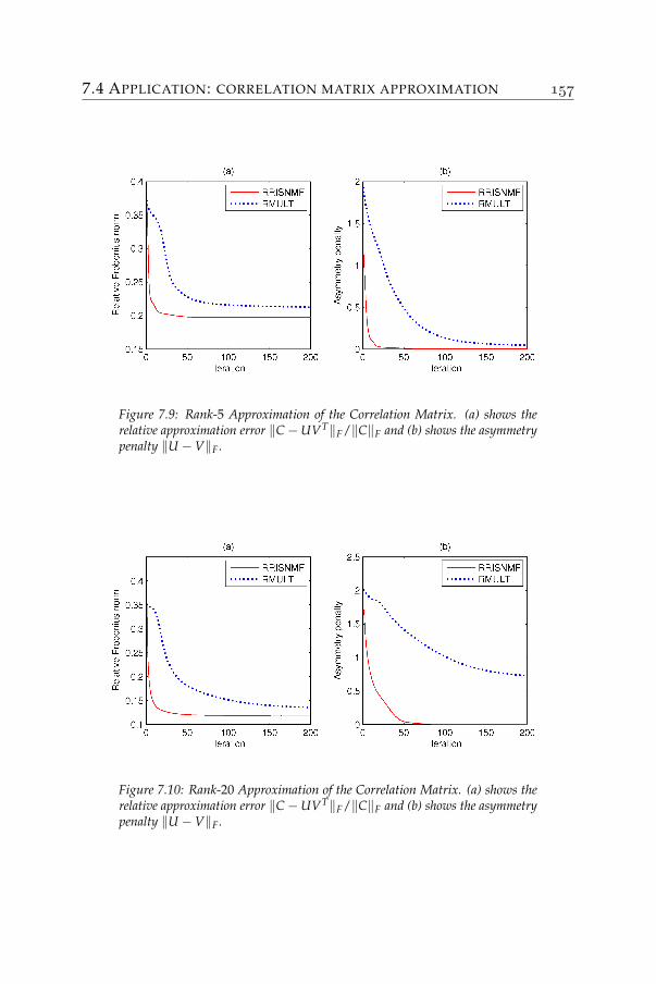
7.4 APPLICATION: CORRELATION MATRIX APPROXIMATION
Figure 7.9: Rank-5 Approximation of the Correlation Matrix. (a) shows therelative approximation error ‖C−UVT‖F/‖C‖F and (b) shows the asymmetrypenalty ‖U −V‖F.
Figure 7.10: Rank-20 Approximation of the Correlation Matrix. (a) shows therelative approximation error ‖C−UVT‖F/‖C‖F and (b) shows the asymmetrypenalty ‖U −V‖F.
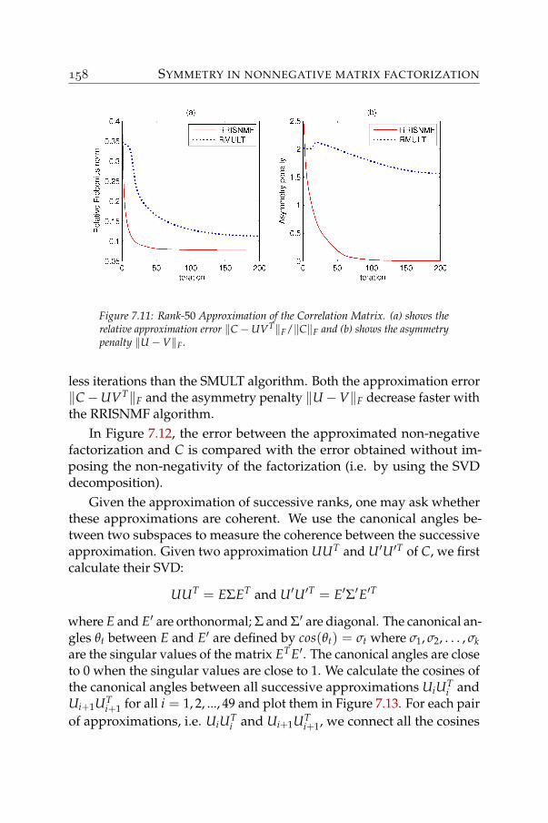
SYMMETRY IN NONNEGATIVE MATRIX FACTORIZATION
Figure 7.11: Rank-50 Approximation of the Correlation Matrix. (a) shows therelative approximation error ‖C−UVT‖F/‖C‖F and (b) shows the asymmetrypenalty ‖U −V‖F.
less iterations than the SMULT algorithm. Both the approximation error‖C−UVT‖F and the asymmetry penalty ‖U−V‖F decrease faster withthe RRISNMF algorithm.
In Figure 7.12, the error between the approximated non-negativefactorization and C is compared with the error obtained without im-posing the non-negativity of the factorization (i.e. by using the SVDdecomposition).
Given the approximation of successive ranks, one may ask whetherthese approximations are coherent. We use the canonical angles be-tween two subspaces to measure the coherence between the successiveapproximation. Given two approximation UUT and U′U′T of C, we firstcalculate their SVD:
UUT = EΣET and U′U′T = E′Σ′E′T
where E and E′ are orthonormal; Σ and Σ′ are diagonal. The canonical an-gles θt between E and E′ are defined by cos(θt) = σt where σ1, σ2, . . . , σkare the singular values of the matrix ETE′. The canonical angles are closeto 0 when the singular values are close to 1. We calculate the cosines ofthe canonical angles between all successive approximations UiUT
i andUi+1UT
i+1 for all i = 1, 2, ..., 49 and plot them in Figure 7.13. For each pairof approximations, i.e. UiUT
i and Ui+1UTi+1, we connect all the cosines
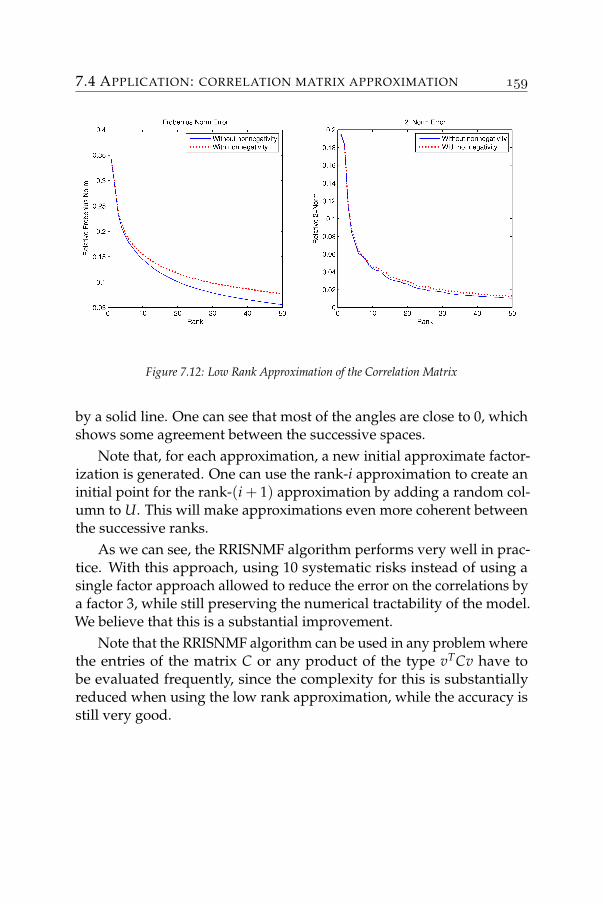
7.4 APPLICATION: CORRELATION MATRIX APPROXIMATION
Figure 7.12: Low Rank Approximation of the Correlation Matrix
by a solid line. One can see that most of the angles are close to 0, whichshows some agreement between the successive spaces.
Note that, for each approximation, a new initial approximate factor-ization is generated. One can use the rank-i approximation to create aninitial point for the rank-(i + 1) approximation by adding a random col-umn to U. This will make approximations even more coherent betweenthe successive ranks.
As we can see, the RRISNMF algorithm performs very well in prac-tice. With this approach, using 10 systematic risks instead of using asingle factor approach allowed to reduce the error on the correlations bya factor 3, while still preserving the numerical tractability of the model.We believe that this is a substantial improvement.
Note that the RRISNMF algorithm can be used in any problem wherethe entries of the matrix C or any product of the type vTCv have tobe evaluated frequently, since the complexity for this is substantiallyreduced when using the low rank approximation, while the accuracy isstill very good.
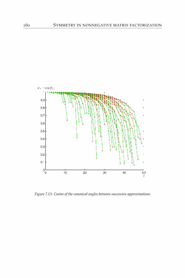
SYMMETRY IN NONNEGATIVE MATRIX FACTORIZATION
Figure 7.13: Cosine of the canonical angles between successive approximations
CONCLUSION
Starting from some problems of data analysis in large graphs, the firstresults of this research came from some large nonnegative matricesrepresenting the adjacency matrix of graphs. Many proposed methodssuch as the Markov Graph Clustering (MCL) [117] work very well forsmall problems. But applying these to large scale problems requirea large memory space and computational cost. This tells us that lowcomplexity should be one of the main criteria considered when choosinga method.
A further study of clustering methods reveals that clustering algo-rithms actually provide a way to reduce the complexity of the data byexploiting the cluster structure. For example, the K−means method [72]represents each group of data points by its centroid. The whole datasetis then represented by the centroids only, which provide a great com-plexity reduction. However, this yields a big approximation error. Theadvantage of K−means methods is that the centroid is always situatedin the proximity of the data and reflects the physical interpretation ofthe represented group.
Returning to large nonnegative matrices, our objective was set to findapproximation algorithms which can yield a small error while keepingthe physical representation of the data. Then the nonnegative matrixfactorization [80] was a perfect starting point. Algorithms proposed bythis paper possess a low complexity and produces nonnegative bases,which matches our expectation. Studying this method, we came to thefollowing conclusions:
• The convergence of these algorithms requires more investigation.One can obtain a non stationary point if zeros are not properly
CONCLUSION
treated, as shown in Section 3.1.
• A nice property of the nonnegative matrix factorization can be es-tablished when using the generalized Kullback-Leibler divergenceas the cost function. It can be seen in Chapter 5 that, the row andcolumn sums are preserved in the approximation.
• Multiplicative rules can be extended to the weighted cases. Andthanks to this, an interesting link is revealed between the mini-mization of the weighted Euclidean distance and the generalizedKullback-Leibler divergence. The use of weights is discussed inChapter 6.
• A special case where a symmetric factorization UUT is requiredlinks the nonnegative matrix factorization to the class of com-pletely positive matrices. While exact methods have exponentialcomplexity, approximative methods can be derived from the al-gorithm of Lee and Seung. This proves useful when applied tothe problem of approximating correlation matrices and clusteringvertices of graphs as shown in Section 7.
While the convergence of the multiplicative rules remains unclear,we seek for alternative methods. We remark that all methods are us-ing the coordinate descent scheme, i.e. only some search directionsare allowed. This breaks down the problem into smaller ones that areusually convex. The popular partition of variables allows us to createsome completely decoupled problems which sometimes can be solvedin parallel. But although the elementary problem is convex, the solutionof the inner loop can be very time consuming. Improvements are madeby replacing the optimal solution of the elementary problem by a subop-timal solution. This does speed up the algorithms but the convergenceproperty is lost.
In the search for a new algorithm, we then propose another way topartition the variables. The approximation matrix UVT is now parti-tioned into a combination of rank-one nonnegative matrices uivT
i . Break-ing the nonnegative matrix factorization problem into smaller problemsaccording to the sub-variables ui’s and vi’s allows us to formulate aclosed form solution for each of the elementary problems. Because theproblem is reduced to a problem of iteratively approximating a residue

CONCLUSION
matrix by a rank-one nonnegative matrix, this method is called Rank-oneResidue Iteration. The development of the method is presented in Chapter4, where a good convergence property is also established. Two otherindependent reports [31] and [49] also proposed this algorithm.
The new algorithm is tested on some numerical experiments to showthat it converges faster than the existing algorithms. Without parameters,it is ready to apply to any application. The algorithm requires at eachiteration only one matrix-vector multiplication, and therefore has a lowcomplexity. We summarize here some other issues around the Rank-oneResidue Iteration:
• It can be applied to other classes of nonnegative approximationssuch as: discrete approximations, sparse approximations, etc. Thechoice of constraints can be different from column to column of Uand V, cfr. Section 4.4.
• Algorithms can be derived for the multilayer nonnegative matrixfactorization (see Section 4.6.1) and the nonnegative tensor factor-ization (cfr. Section 4.6.2). The numerical experiments at the endof Chapter 4 suggest that the nonnegative tensor factorization canprovide comparable results with that of the SVD, given the samecompression rate.
• It can be adapted to take into account weights, see Section 6.2.2and to construct the symmetric factorizations of type UUT andUSUT, cfr. Section 7.2.2 and Section 7.2.2.
There remains several open issues. The first one is the convergence ofthe multiplicative rules. While the algorithm may return non stationarypoints, it is still uncertain about whether this is solely due to the finiteprecision of the computer. Section 3.1 points out that it is probably truethat starting from a positive point, with a clever treatment of the zeros,one could improve the convergence of this elegant algorithm.
The second issue is about the existence of many local minima. Whenrepresenting the rank-k matrix by the product UVT with appropriatesizes, too many degrees of freedom are added to the problem. Thiscreates many local minima. Current applications often take one of theselocal minima ignoring the others. It is shown through an example in
CONCLUSION
Section 7.2.2 that not every local minimum is good. While the use ofnonnegative matrix factorization generates an asymmetric approxima-tion with large error, this is shown that by controlling the minimizationprocedure to a symmetric factorization, the result is significantly im-proved.
Studying these issues definitely opens many promising researchdirections. Here are a number of issues that could bring many immediateconsequences:
• designing good and cheap techniques to initialize any nonnegativematrix factorization algorithm,
• creating a heuristic of which constraints need to be imposed toobtain a desired approximation,
• testing the block version of RRI algorithm. At the time of writing,it is possible to create updates for two columns of U (or of V) atthe same time. We should then ask if it is possible to update evenmore columns simultaneously and in which order,
• searching for direct methods for the symmetric and semi-symmetr-ic nonnegative matrix factorization to avoid the use of regulariza-tion,
• studying higher dimensional analysis such as the nonnegativetensor factorization,
• and searching for methods with a algorithmic complexity bound.
BIBLIOGRAPHY
[1] A.V. Aho, J.E. Hopcroft, and J.D. Ullman. The design and analysis ofcomputer algorithms. Addison-Wesley Reading, MA, 1974.
[2] R. Albright, J. Cox, D. Duling, A.N. Langville, and C.D. Meyer.Algorithms, initializations, and convergence for the nonnegativematrix factorization. Preprint, 2006.
[3] S. Ambikkumar and S.W. Drury. A reverse Hadamard inequality.Linear Algebra and its Applications, 247:83–95, 1996.
[4] M. Avriel. Nonlinear Programming: analysis and methods. DoverPublications, 2003.
[5] B.W. Bader and T.G. Kolda. Efficient MATLAB computations withsparse and factored tensors. Technical Report SAND2006-7592,Sandia National Laboratories, Albuquerque, NM and Livermore,CA, Dec. 2006.
[6] A. Banerjee, I. Dhillon, J. Ghosh, S. Merugu, and D.S. Modha. Ageneralized maximum entropy approach to bregman co-clusteringand matrix approximation. In Proceedings of the 2004 ACM SIGKDDInternational Conference on Knowledge Discovery and Data Mining,pages 509–514, 2004.
[7] F. Barioli and A. Berman. The maximal cp-rank of rank k com-pletely positive matrices. Linear Algebra and its Applications, 363:17–33, 2003.
[8] A. Berman and R.J. Plemmons. Nonnegative matrices in the mathe-matical sciences. Siam, 1994.
BIBLIOGRAPHY
[9] A. Berman and U.G. Rothblum. A note on the computation of theCP-rank. Linear Algebra and its Applications, 419(1):1–7, 2006.
[10] A. Berman and N. Shaked-Monderer. The completely positive matri-ces. World Scientific, 2003.
[11] M.W. Berry and M. Browne. Email surveillance using non-negative matrix factorization. Computational and MathematicalOrganization Theory, 11(3):249–264, 2005.
[12] M.W. Berry, M. Browne, A.N. Langville, V.P. Pauca, and R.J. Plem-mons. Algorithms and applications for approximate nonnegativematrix factorization. Computational Statistics and Data Analysis,52(1):155–173, 2007.
[13] D.P. Bertsekas. Nonlinear programming. Athena Scientific Belmont,Mass, 1999.
[14] D.P. Bertsekas, A. Nedic, and A.E. Ozdaglar. Convex analysis andoptimization. Athena Scientific Belmont, Mass, 2003.
[15] I. Biederman. Recognition-by-components: A theory of humanimage understanding. Psychological Review, 94(2):115–147, 1987.
[16] M. Biggs, A. Ghodsi, and S. Vavasis. Nonnegative matrix factor-ization via rank-one downdate. University of Waterloo, Preprint,2007.
[17] A. Bjorck. Numerical methods for least squares problems. SIAMPhiladelphia, 1996.
[18] V.D. Blondel, A. Gajardo, M. Heymans, P. Senellart, andP. Van Dooren. A measure of similarity between graph vertices:Applications to synonym extraction and web searching. SIAMreview, 46(4):647–666, 2004.
[19] V.D. Blondel, N.-D. Ho, and P. Van Dooren. Nonnegative matrixfactorization - applications and extensions. Technical Report 005-35, Cesame. University catholique de Louvain. Belgium. 2005,2005.
BIBLIOGRAPHY
[20] C. Boutsidis and E. Gallopoulos. SVD based initialization: a headstart for nonnegative matrix factorization. Pattern Recognition,41(4):1350–1362, 2008.
[21] S.P. Boyd and L. Vandenberghe. Convex optimization. CambridgeUniversity Press, 2004.
[22] U. Brandes, M. Gaertler, and D. Wagner. Experiments on graphclustering algorithms. In Proceedings of the 11th Annual EuropeanSymposium on Algorithms (ESA 2003), pages 568–579. Springer,2003.
[23] S. Brin and L. Page. The anatomy of a large-scale hypertextualWeb search engine. Computer Networks and ISDN Systems, 30(1-7):107–117, 1998.
[24] R. Bro and S. De Jong. A fast non-negativity constrained leastsquares algorithm. Journal of Chemometrics, 11(5):393–401, 1997.
[25] M. Catral, L. Han, M. Neumann, and RJ Plemmons. On reducedrank nonnegative matrix factorization for symmetric nonnegativematrices. Linear Algebra and its Applications, 393:107–126, 2004.
[26] M. Chu, F. Diele, R. Plemmons, and S. Ragni. Optimality, com-putation and interpretation of nonnegative matrix factorizations.SIAM Journal on Matrix Analysis, 2004.
[27] M.T. Chu, R.E. Funderlic, and R.J. Plemmons. Structured low rankapproximation. Linear Algebra and its Applications, 366:157–172,2003.
[28] A. Cichocki, S. Amari, and R. Zdunek. Extended SMART algo-rithms for non-negative matrix factorization. In Proceeding of theEighth International Conference on Artificial Intelligence and Soft Com-puting, pages 548–562, 2006.
[29] A. Cichocki and R. Zdunek. Multilayer nonnegative matrix factor-ization. Electronics Letters, 42(16):947–948, 2006.
[30] A. Cichocki, R. Zdunek, and S. Amari. Csiszar’s divergencesfor non-negative matrix factorization: family of new algorithms.Lecture Notes in Computer Science, 3889:32–39, 2006.
BIBLIOGRAPHY
[31] A. Cichocki, R. Zdunek, and S. Amari. Hierarchical ALS algo-rithms for nonnegative matrix and 3D tensor factorization. InProceedings of 7th International Conference on Independent Compo-nent Analysis and Signal Separation, ICA 2007, London, UK, pages169–176, 2007.
[32] A. Cichocki, R. Zdunek, and S. Amari. Nonnegative matrix andtensor factorization. Signal Processing Magazine, IEEE, 25(1):142–145, 2008.
[33] J.E. Cohen and U.G. Rothblum. Nonnegative ranks, decomposi-tions, and factorizations of nonnegative matrices. Linear Algebraand its Applications, 190:149–168, 1993.
[34] M. Cooper and J. Foote. Summarizing video using non-negativesimilarity matrix factorization. In IEEE Multimedia Signal Process-ing Workshop, pages 25–28, 2002.
[35] A. Cutler and L. Breiman. Archetypal Analysis. Technometrics,36(4):338–347, 1994.
[36] I.S. Dhillon and S. Sra. Generalized nonnegative matrix approx-imations with Bregman divergences. In Proceeding of the NeuralInformation Processing Systems (NIPS) Conference, Vancouver, BC,2005.
[37] C. Ding, X. He, and H. Simon. On the equivalence of nonnegativematrix factorization and spectral clustering. In Proceedings of SIAMData Mining Conference, pages 606–610, 2005.
[38] C. Ding, T. Li, and M.I. Jordan. Convex and semi-nonnegativematrix factorizations. Technical Report 60428, Lawrence BerkeleyNational Laboratory, 2006.
[39] D. Donoho and V. Stodden. When does non-negative matrixfactorization give a correct decomposition into parts? In Advancesin Neural Information Processing Systems, volume 16, pages 1141–1148, 2004.
[40] L. Elsner, R. Nabben, and M. Neumann. Orthogonal bases thatlead to symmetric nonnegative matrices. Linear Algebra and itsApplications, 271(1-3):323–343, 1998.
BIBLIOGRAPHY
[41] J. Falkner, F. Rendl, and H. Wolkowicz. A computational studyof graph partitioning. Mathematical Programming, 66(1):211–239,1994.
[42] L. Finesso and P. Spreij. Nonnegative matrix factorization andi-divergence alternating minimization. Linear Algebra and its Appli-cations, 416:270–287, 2006.
[43] R. Fisher. Iris flower dataset.http://en.wikipedia.org/wiki/Iris_flower_data_set.
[44] V. Franc, V. Hlavác, and M. Navara. Sequential coordinate-wisealgorithm for the non-negative least squares problem. In CAIP2005: Computer Analysis of Images and Patterns, volume 3691, pages407–414, September 2005.
[45] H.T. Gao, T.H. Li, K. Chen, W.G. Li, and X. Bi. Overlappingspectra resolution using non-negative matrix factorization. Talanta,66(1):65–73, 2005.
[46] Y. Gao and G. Church. Improving molecular cancer class discoverythrough sparse non-negative matrix factorization. Bioinformatics,21(21):3970–3975, 2005.
[47] E. Gaussier and C. Goutte. Relation between PLSA and NMFand implications. In Proceedings of the 28th Annual InternationalACM SIGIR Conference on Research and Development in InformationRetrieval, pages 601–602. ACM Press New York, NY, USA, 2005.
[48] N. Gillis. Approximation et sous-approximation de matrices parfactorisation positive: algorithmes, complexité et applications.M.S. Thesis, Université catholique de Louvain, 2007.
[49] N. Gillis and François Glineur. Nonnegative matrix factorizationand underapproximation. Preprint, 2008.
[50] G. Golub and C. F. Van Loan. Matrix computations.3rd ed. Baltimore,The Johns Hopkins Univ. Press. xxvii, 694 p. , 1996.
[51] E.F. Gonzales and Y. Zhang. Accelerating the Lee-Seung algorithmfor nonnegative matrix factorization. Technical Report TR-05-02,
BIBLIOGRAPHY
Department of Computational and Applied Mathematics, RiceUniversity, 2005, 2005.
[52] L. Grippo and M. Sciandrone. On the convergence of the blocknonlinear gauss-seidel method under convex constraints. Opera-tions Research Letters, 26(3):127–136, 2000.
[53] D. Guillamet, M. Bressan, and J. Vitrià. A weighted nonnegativematrix factorization for local representations. In IEEE ComputerSociety Conference on Compute Vision and Pattern Recognition, pages942–947, 2001.
[54] D. Guillamet and J. Vitria. Non-negative matrix factorization forface recognition. Lecture Notes on Artificial Intelligence, 2504:336–344, 2002.
[55] D. Guillamet, J. Vitrià, and B. Schiele. Introducing a weightednon-negative matrix factorization for image classification. PatternRecognition Letters, 24(14):2447–2454, 2003.
[56] M. Heiler and C. Schnörr. Learning sparse representations by non-negative matrix factorization and sequential cone programming.The Journal of Machine Learning Research, 7:1385–1407, 2006.
[57] N.J. Higham. Computing a nearest symmetric positive semidefi-nite matrix. Linear Algebra Application, 103:103–118, 1988.
[58] N.J. Higham, MJC Gover, and S. Barnett. Matrix nearness prob-lems and applications. Applications of Matrix Theory, pages 1–27,1989.
[59] N.-D. Ho, V. Blondel, and P. Van Dooren. Weighted nonnegativematrix factorization and face feature extraction. Submitted to Imageand Vision Computing, 2007.
[60] N.-D. Ho and F. Cédrick. Lexical similarity based on quantity ofinformation exchanged - synonym extraction. In Proceedings of theResearch Informatics Vietnam-Francophony, Hanoi, Vietnam, pages193–198, 2004.
BIBLIOGRAPHY
[61] N.-D. Ho and P. Van Dooren. On the pseudo-inverse of the Lapla-cian of a bipartite graph. Applied Mathematics Letters, 18(8):917–922,2005.
[62] N.-D. Ho, P. Van Dooren, and V.D. Blondel. Descent algorithmsfor nonnegative matrix factorization. Technical Report 2007-57,Cesame. University catholique de Louvain. Belgium. 2007. Toappear in Numerical Linear Algebra in Signals, Systems and Control.,2007.
[63] N.-D. Ho, P. Van Dooren, and V.D. Blondel. Descent algorithmsfor Nonnegative Matrix Factorization. Survey paper. To appear inNumerical Linear Algebra in Signals, Systems and Control, 2008.
[64] T. Hofmann. Probabilistic latent semantic indexing. In Proceedingsof the 22nd Annual International ACM SIGIR Conference on Researchand Development in Information Retrieval, pages 50–57. ACM PressNew York, NY, USA, 1999.
[65] T. Hofmann. Unsupervised learning by probabilistic latent seman-tic analysis. Machine Learning, 42(1/2):177–196, 2001.
[66] R. A. Horn and C. R. Johnson. Matrix analysis. Cambridge Univer-sity Press. XIII, 561 p., 1985.
[67] R. A. Horn and C. R. Johnson. Topics in matrix analysis. CambridgeUniversity Press. viii, 607 p. , 1991.
[68] P. O. Hoyer. Non-negative matrix factorization with sparsenessconstraints. Journal of Machine Learning Research, 5:1457–1469, 2004.
[69] P.O. Hoyer. Non-negative sparse coding. In Proceedings of the 200212th IEEE Workshop on Neural Networks for Signal Processing, pages557–565, 2002.
[70] S. Impedovo, L. Ottaviano, and S. Occhinegro. Optical characterrecognition–a survey. Internatioanl Journal of Pattern Recoginitionand Artificial Intelligence, 5(1):1–24, 1991.
[71] C.T. Ireland and S. Kullback. Contingency tables with givenmarginals. Biometrika, 55(1):179–188, 2001.
BIBLIOGRAPHY
[72] A.K. Jain and R.C. Dubes. Algorithms for clustering data. Prentice-Hall, Inc. Upper Saddle River, NJ, USA, 1988.
[73] M. Kaykobad. On nonnegative factorization of matrices. LinearAlgebra and its Applications, 96:27–33, 1987.
[74] M.H.V. Keenan. Fast algorithm for the solution of large-scalenon-negativity-constrained least squares problems. Chemometrics,18:441–450, 2004.
[75] P. A. Knight and D. Ruiz. A fast algorithm for matrix balancing.In Web Information Retrieval and Linear Algebra Algorithms, 2007.
[76] T.G. Kolda and D.P. O’Leary. A semidiscrete matrix decompo-sition for latent semantic indexing information retrieval. ACMTransactions on Information Systems (TOIS), 16(4):322–346, 1998.
[77] R. Kompass. A generalized divergence measure for nonnegativematrix factorization. Neural Computation, 19(3):780–791, 2007.
[78] S. Kullback. Information theory and statistics. Courier Dover Publi-cations, 1997.
[79] C.L. Lawson and R.J. Hanson. Solving least squares problems.Prentice-Hall Englewood Cliffs, NJ, 1974.
[80] D. D. Lee and H. S. Seung. Learning the parts of objects by non-negative matrix factorization. Nature, 401, 1999.
[81] D. D. Lee and H. S. Seung. Algorithms for non-negative matrixfactorization. In Neural Information Processing Systems, pages 556–562, 2000.
[82] D.D. Lee and H.S. Seung. Unsupervised learning by convex andconic coding. Advances in Neural Information Processing Systems,9:515–521, 1997.
[83] S.Z. Li, X.W. Hou, H.J. Zhang, and Q.S. Cheng. Learning spatiallylocalized, parts-based representation. In Proceedings of IEEE Conf.Computer Vision and Pattern Recognition, pages 1–6, 2001.
BIBLIOGRAPHY
[84] J. Liang and D. Fairley. Validation of an efficient non-negativematrix factorization method and its preliminary application inCentral California. Atmospheric environment, 40(11):1991–2001,2006.
[85] C.-J. Lin. On the convergence of multiplicative update algorithmsfor non-negative matrix factorization. IEEE Transactions on NeuralNetworks, 2007. To appear.
[86] C.-J. Lin. Projected gradient methods for non-negative matrixfactorization. Neural Computation, 2007. To appear.
[87] D.G. Luenberger. Linear and nonlinear programming. Springer, 2003.
[88] J. MacQueen. Some methods for classification and analysis of mul-tivariate observations. Proceedings of the Fifth Berkeley Symposiumon Mathematical Statistics and Probability, 1(281-297):14, 1967.
[89] M. Merritt and Y. Zhang. Interior-point gradient method forlarge-scale totally nonnegative least squares problems. Journal ofOptimization Theory and Applications, 126(1):191–202, 2005.
[90] E. Moore Gordon. Cramming more components onto integratedcircuits. Electronics, 38(8):114–117, 1965.
[91] N. Murata, T. Takenouchi, T. Kanamori, and S. Eguchi. Infor-mation geometry of U-Boost and bregman divergence. NeuralComputation, 16(7):1437–1481, 2004.
[92] Y. Nesterov. Smooth minimization of non-smooth functions. Math-ematical Programming, 103(1):127–152, 2005.
[93] J. Nocedal and S.J. Wright. Numerical optimization. Springer, 1999.
[94] P.D. O’Grady and B.A. Pearlmutter. Convolutive non-negativematrix factorisation with a sparseness constraint. In Proceedingsof the 2006 16th IEEE Signal Processing Society Workshop on, pages427–432, 2006.
[95] Paatero P. Least squares formulation of robust non-negative factoranalysis. Chemometrics and Intelligent Laboratory Systems, 37:23–35,1997.
BIBLIOGRAPHY
[96] P. Paatero. A weighted non-negative least squares algorithm forthree-way ’parafac’ factor analysis. Chemometrics and IntelligentLaboratory Systems, 38(2):223–242, 1997.
[97] P. Paatero and U. Tapper. Positive matrix factorization: a non-negative factor model with optimal utilization of error estimatesof data values. Environmetrics, 5(1):111–126, 1994.
[98] A. Pascual-Montano, J.M. Carazo, K. Kochi, D. Lehmann, andR.D. Pascual-Marqui. Nonsmooth nonnegative matrix factoriza-tion (nsNMF). IEEE Transactions on Pattern Analysis and MachineIntelligence, 28(3):403–415, 2006.
[99] V.P. Pauca, J. Piper, and R.J. Plemmons. Nonnegative matrix factor-ization for spectral data analysis. Linear Algebra and its Applications,416(1):29–47, 2006.
[100] L.R. Rabiner. A tutorial on hidden Markov models and selected ap-plications in speech recognition. Proceedings of the IEEE, 77(2):257–286, 1989.
[101] J. Renegar. On the computational complexity and geometry of thefirst-order theory of the reals. Par I: Introduction. Preliminaries.The geometry of semi-algebraic sets. The decision problem forthe existential theory of the reals. Journal of Symbolic Computation,13(3):255–299, 1992.
[102] R.T. Rockafellar. Convex analysis. Princeton University Press, 1970.
[103] F. Shahnaz, M.W. Berry, V.P. Pauca, and R.J. Plemmons. Documentclustering using nonnegative matrix factorization. InformationProcessing & Management, 42(2):373–386, 2006.
[104] A. Shashua and T. Hazan. Non-negative tensor factorization withapplications to statistics and computer vision. In Proceedings of theInternational Conference on Machine Learning (ICML), pages 792–799,2005.
[105] A. Shashua, R. Zass, and T. Hazan. Multi-way clustering usingsuper-symmetric non-negative tensor factorization. In Proceedingof European Conference on Computer Vision, pages 595–608. Springer,2006.
BIBLIOGRAPHY
[106] R. Sinkhorn. A relationship between arbitrary positive matricesand doubly stochastic. The Annals of Mathematical Statistics, 35:876–879, 1964.
[107] R. Sinkhorn. Diagonal equivalence to matrices with prescribedrow and rolumn sums. The American Mathematical Monthly,74(4):402–405, 1967.
[108] P. Smaragdis and J.C. Brown. Non-negative matrix factorizationfor polyphonic music transcription. 2003 IEEE Workshop on Appli-cations of Signal Processing to Audio and Acoustics, pages 177–180,2003.
[109] A.W.M. Smeulders, M. Worring, S. Santini, A. Gupta, and R. Jain.Content-based image retrieval at the end of the early years.IEEE Transactions on Pattern Analysis and Machine Intelligence,22(12):1349–1380, 2000.
[110] S. Sra and I.S. Dhillon. Nonnegative matrix approximation: al-gorithms and applications. Technical Report Tr-06-27, ComputerSciences, University of Texas at Austin, 2006, 2006.
[111] N. Srebro and T. Jaakkola. Weighted low-rank approximations.In Proceedings of the Twentieth International Conference on MachineLearning, pages 720–727, 2003.
[112] Credit Suisse. CreditRisk+. Credit Suisse Financial Products(1997),http://www.csfb.com/creditrisk, 1997.
[113] A. Tarski. A decision method for elementary algebra and geometry.University of California Press, 1951.
[114] J. Tropp. Literature survey: nonnegative matrix factorization.University of Texas at Asutin, preprint, 2003.
[115] J. M. Van Den Hof. Realization of positive linear systems. LinearAlgebra and its Applications, 256(1–3):287–308, 1997.
[116] J.M. Van Den Hof and J.H. Van Schuppen. Positive matrix fac-torization via extremal polyhedral cones. Linear Algebra and itsApplications, 293(1-3):171–186, 1999.
BIBLIOGRAPHY
[117] S.M. van Dongen. Graph Clustering by Flow Simulation. PhD thesis,University of Utrecht, 2000.
[118] C.F. Van Loan. The ubiquitous Kronecker product. Journal ofComputational and Applied Mathematics, 123(1-2):85–100, 2000.
[119] A. Vandendorpe, N.D. Ho, S. Vanduffel, and P. Van Dooren. Onthe parameterization of the CreditRisk model for estimating creditportfolio risk. Accepted for publication in Insurance: Mathematics andEconomics, 2007.
[120] B. Vanluyten, J.C. Willems, and B. De Moor. Matrix factorizationand stochastic state representations. 2006 45th IEEE Conference onDecision and Control, pages 4188–4193, 2006.
[121] S.A. Vavasis. On the complexity of nonnegative matrix factoriza-tion. eprint arXiv: 0708.4149, 2007.
[122] Y. Wang, Y. Jia, C. Hu, and M. Turk. Fisher non-negative matrixfactorization for learning local features. In Proceedings of AsianConference on Computer Vision, 2004.
[123] D.S. Watkins. Fundamentals of matrix computations. John Wiley &Sons, Inc. New York, NY, USA, 1991.
[124] M. Welling and M. Weber. Positive tensor factorization. PatternRecognition Letters, 22(12):1255–1261, 2001.
[125] S. Wild. Seeding non-negative matrix factorizations with thespherical K-Means clustering. M.S. Thesis, University of Colorado,2003.
[126] S. Wild, J. Curry, and A. Dougherty. Motivating non-negativematrix factorizations. In Proceedings of Eighth SIAM Conference onApplied Linear Algebra, Philadelphia, 2003.
[127] S. Wild, J. Curry, and A. Dougherty. Improving non-negativematrix factorizations through structured initialization. Patternrecognition, 37(11):2217–2232, 2004.

BIBLIOGRAPHY
[128] W. Xu, X. Liu, and Y. Gong. Document clustering based on non-negative matrix factorization. In Proceedings of the 26th AnnualInternational ACM SIGIR Conference on Research and Developmentin Informaion Retrieval, pages 267–273. ACM Press New York, NY,USA, 2003.