Chapter

11

Elementary Statistics

Larson Farber

Nonparametric Tests

The Sign Test

Section 11.1

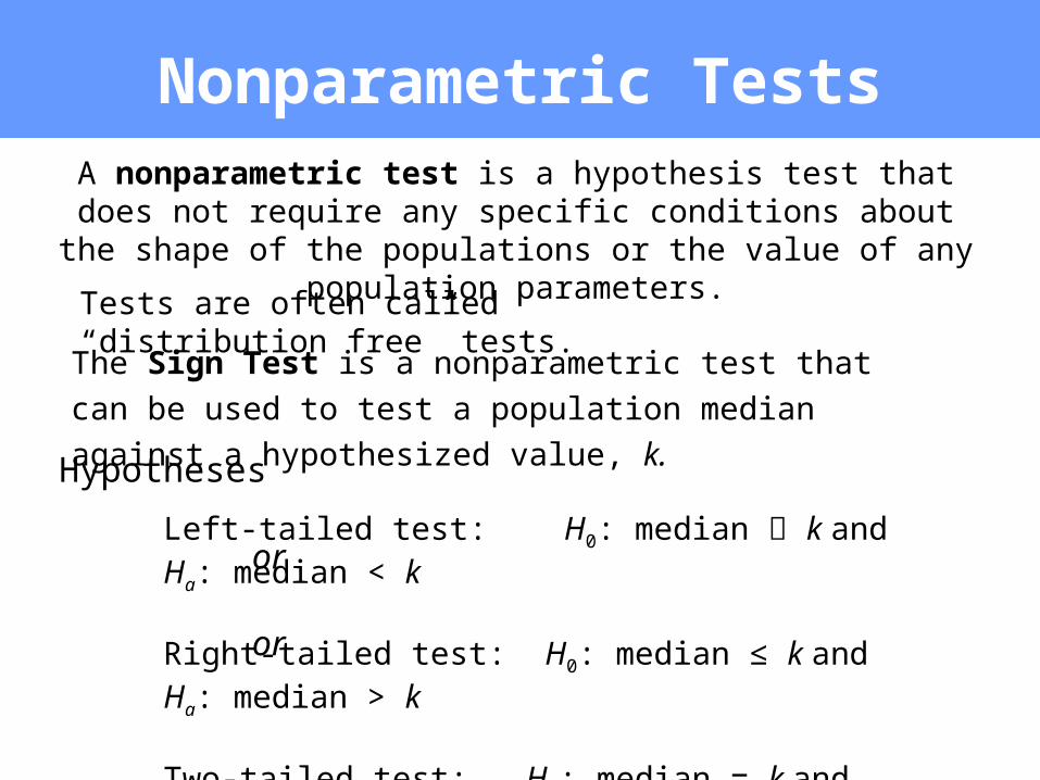
Left-tailed test: H0: median k andHa: median < k

Right-tailed test: H0: median ≤ k and Ha: median > k

Two-tailed test: H0: median = k and Ha: median k

Nonparametric TestsA nonparametric test is a hypothesis test that does not require any specific conditions about the shape of the populations or the

value of any population parameters.

Tests are often called “distribution free” tests.

The Sign Test is a nonparametric test that can be used to

test a population median against a hypothesized value, k.

Hypotheses

or

or

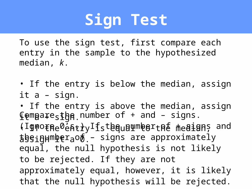
Sign TestTo use the sign test, first compare each entry in the sample to the hypothesized median, k.

• If the entry is below the median, assign it a – sign. • If the entry is above the median, assign it a + sign.• If the entry is equal to the median, assign it a 0.

Compare the number of + and – signs. (Ignore 0’s.) If the number of + signs and the number of – signs are approximately equal, the null hypothesis is not likely to be rejected. If they are not approximately equal, however, it is likely that the null hypothesis will be rejected.

Sign Test

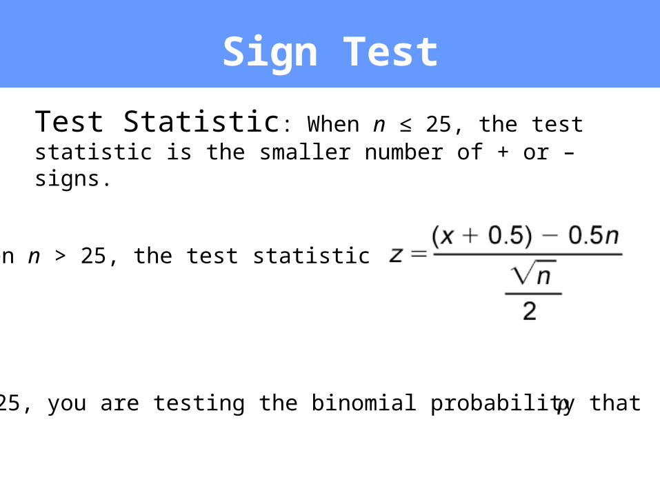
Test Statistic: When n ≤ 25, the test statistic is the smaller number of + or – signs.

When n > 25, the test statistic is:

For n > 25, you are testing the binomial probability that = 0.50.

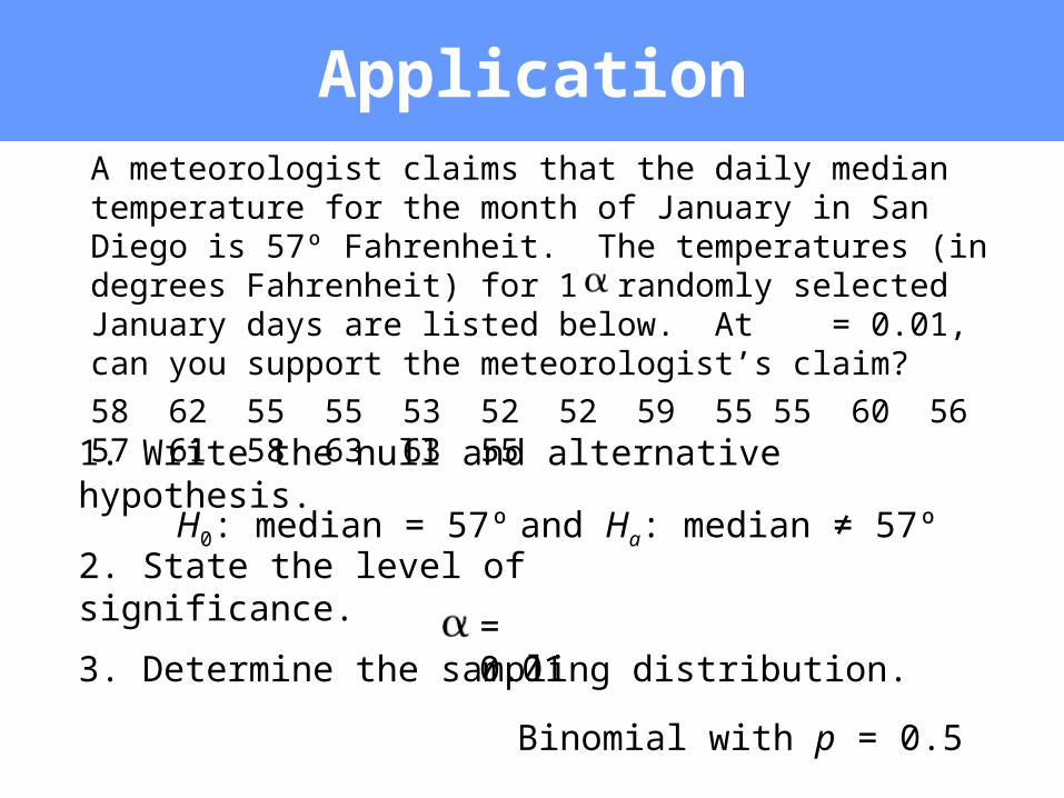
ApplicationA meteorologist claims that the daily median temperature for the month of January in San Diego is 57º Fahrenheit. The temperatures (in degrees Fahrenheit) for 18 randomly selected January days are listed below. At = 0.01, can you support the meteorologist’s claim?

58 62 55 55 53 52 52 59 55 55 60 56 57 61 58 63 63 55

1. Write the null and alternative hypothesis.

H0: median = 57º and Ha: median ≠ 57º

2. State the level of significance.= 0.01

3. Determine the sampling distribution.

Binomial with p = 0.5

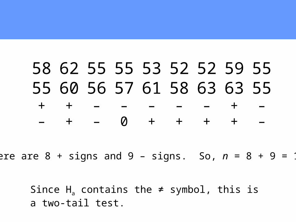
Since Ha contains the ≠ symbol, this is a two-tail test.

There are 8 + signs and 9 – signs. So, n = 8 + 9 = 17.

5855+–

6260++

5556––

5557–0

5361–+

5258–+

5263–+

5963++

5555––

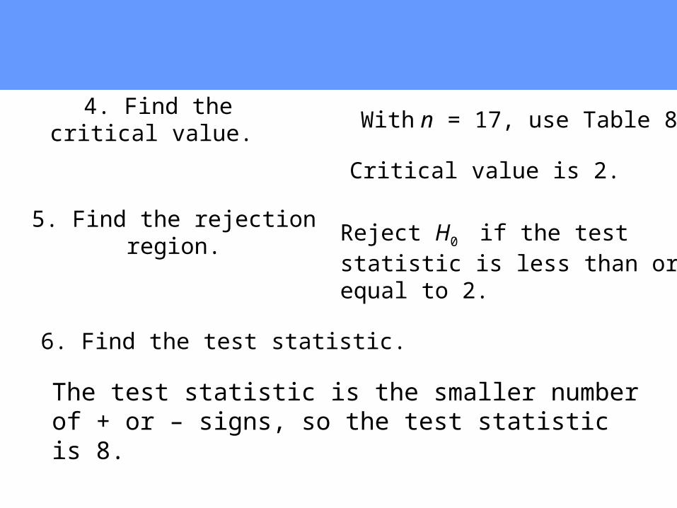
6. Find the test statistic.

5. Find the rejection region.

4. Find the critical value. With n = 17, use Table 8

Critical value is 2.

Reject H0 if the teststatistic is less than orequal to 2.

The test statistic is the smaller number of + or – signs, so the test statistic is 8.

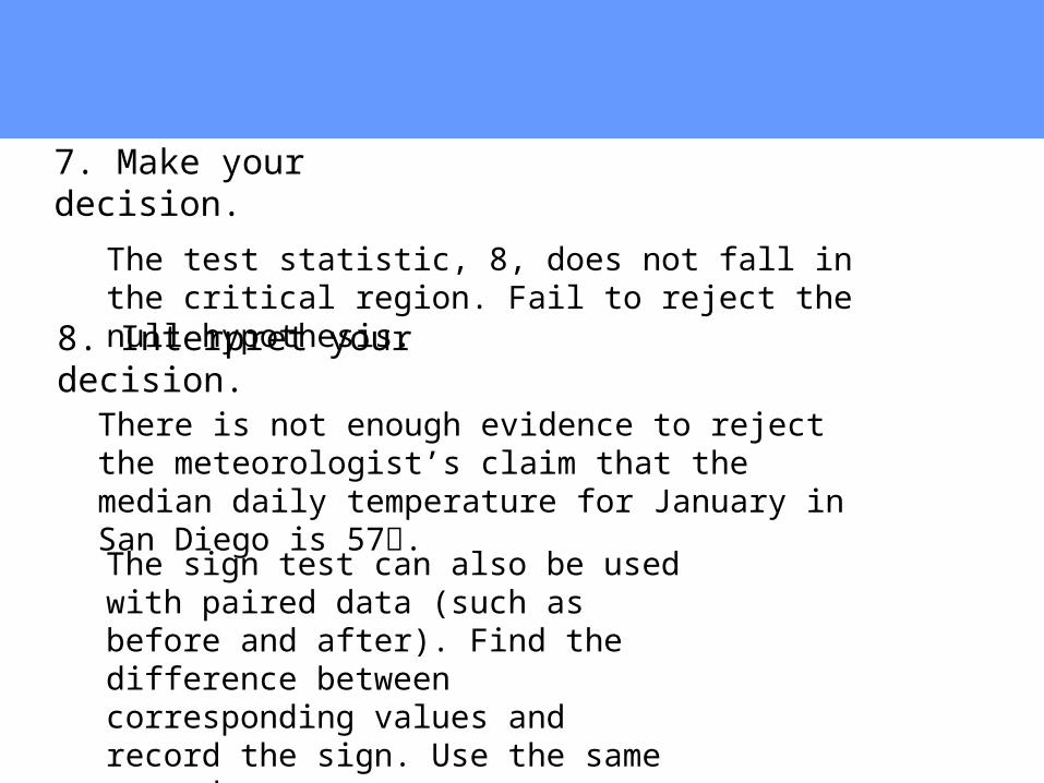
7. Make your decision.

8. Interpret your decision.

The test statistic, 8, does not fall in the critical region. Fail to reject the null hypothesis.

There is not enough evidence to reject the meteorologist’s claim that the median daily temperature for January in San Diego is 57.

The sign test can also be used with paired data (such as before and after). Find the difference between corresponding values and record the sign. Use the same procedure.

The Wilcoxon Test

Section 11.2

Wilcoxon Signed-Rank Test

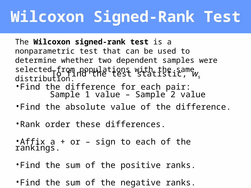
The Wilcoxon signed-rank test is a nonparametric test that can be used to determine whether two dependent samples were selected from populations with the same distribution.

•Find the difference for each pair:Sample 1 value – Sample 2 value

•Find the absolute value of the difference.

•Rank order these differences.

•Affix a + or – sign to each of the rankings.

•Find the sum of the positive ranks.

•Find the sum of the negative ranks.

•Select the smaller of the absolute values of the sums.

To find the test statistic, ws

Application

The table shows the daily headache hours suffered by 12 patients before and after receiving a new drug for seven weeks. At = 0.01, is there enough evidence to conclude that the new drug helped to reduce daily headache hours?

1. Write the null and alternative hypothesis.

2. State the level of significance.

= 0.01

H0: The headache hours after using the new drug are at least as long as before using the drug. Ha: The new drug reduces headache hours. (Claim)

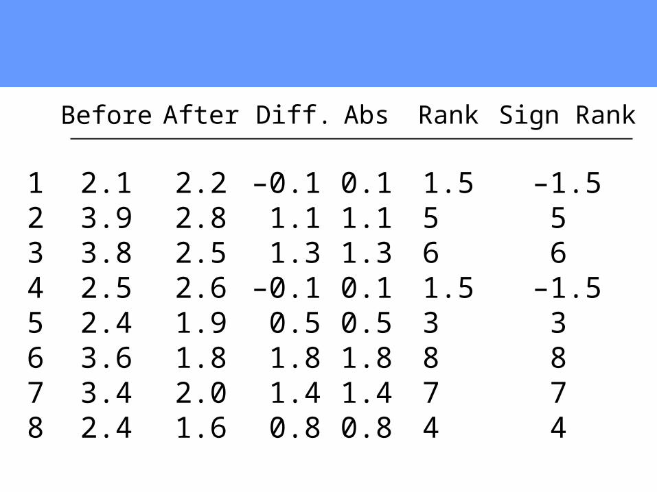
12345678

2.13.93.82.52.43.63.42.4

Before

2.22.82.52.61.91.82.01.6

After

–0.11.11.3

–0.10.51.81.40.8

Diff.

0.11.11.30.10.51.81.40.8

Abs

1.55.06.01.53.08.07.04.0

Rank

–1.55.06.0

–1.53.08.07.04.0

Sign Rank

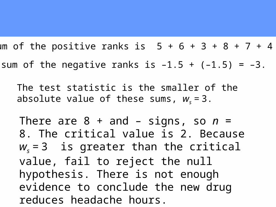
The sum of the positive ranks is 5 + 6 + 3 + 8 + 7 + 4 = 33.

The sum of the negative ranks is –1.5 + (–1.5) = –3.

The test statistic is the smaller of the absolute value of these sums, ws = 3.

There are 8 + and – signs, so n = 8. The critical value is 2. Because ws = 3 is greater than the critical value, fail to reject the null hypothesis. There is not enough evidence to conclude the new drug reduces headache hours.

Wilcoxon Rank-Sum Test

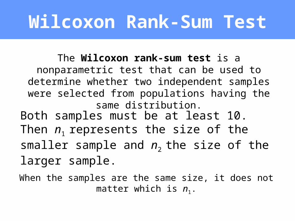
The Wilcoxon rank-sum test is a nonparametric test that can be used to determine whether two independent

samples were selected from populations having the same distribution.

Both samples must be at least 10. Then n1

represents the size of the smaller sample and n2

the size of the larger sample.

When the samples are the same size, it does not matter which is n1.

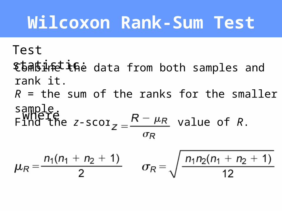
Wilcoxon Rank-Sum Test

Test statistic:Combine the data from both samples and rank it. R = the sum of the ranks for the smaller sample. Find the z-score for the value of R.

where

The Kruskal-Wallis Test

Section 11.3

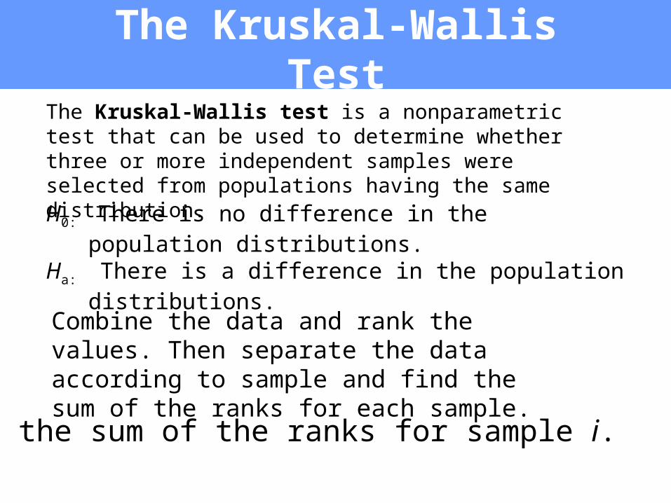
The Kruskal-Wallis TestThe Kruskal-Wallis test is a nonparametric test that can be used to determine whether three or more independent samples were selected from populations having the same distribution.

H0: There is no difference in the population distributions.Ha: There is a difference in the population distributions.

Combine the data and rank the values. Then separate the data according to sample and find the sum of the ranks for each sample.

Ri = the sum of the ranks for sample i.

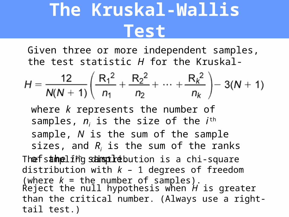
The sampling distribution is a chi-square distribution with k – 1 degrees of freedom (where k = the number of samples).

Given three or more independent samples, the test statistic H for the Kruskal-Wallis test is:

where k represents the number of samples, ni is the size of the i

th sample, N is the sum of the sample sizes, and Ri is the sum of the ranks of the i

th sample.

Reject the null hypothesis when H is greater than the critical number. (Always use a right-tail test.)

The Kruskal-Wallis Test

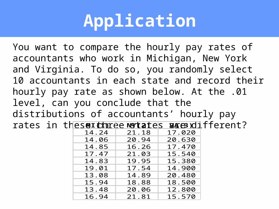
ApplicationYou want to compare the hourly pay rates of accountants who work in Michigan, New York and Virginia. To do so, you randomly select 10 accountants in each state and record their hourly pay rate as shown below. At the .01 level, can you conclude that the distributions of accountants’ hourly pay rates in these three states are different?

MI(1) NY(2) VA(3)14.24 21.18 17.02014.06 20.94 20.63014.85 16.26 17.47017.47 21.03 15.54014.83 19.95 15.38019.01 17.54 14.90013.08 14.89 20.48015.94 18.88 18.50013.48 20.06 12.80016.94 21.81 15.570

= 0.01

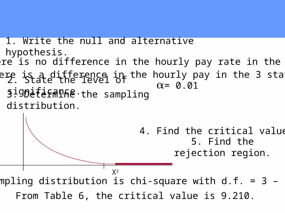
H0 : There is no difference in the hourly pay rate in the 3 states.Ha : There is a difference in the hourly pay in the 3 states.

1. Write the null and alternative hypothesis.

2. State the level of significance.

The sampling distribution is chi-square with d.f. = 3 – 1 = 2.

From Table 6, the critical value is 9.210.

5. Find the rejection region.

4. Find the critical value.

3. Determine the sampling distribution.

X2

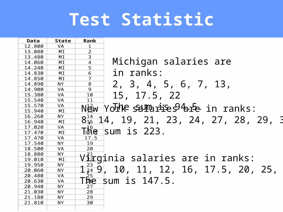
Test StatisticData State Rank

12.800 VA 113.080 MI 213.480 MI 314.060 MI 414.240 MI 514.830 MI 614.850 MI 714.890 NY 814.900 VA 915.380 VA 1015.540 VA 1115.570 VA 1215.940 MI 1316.260 NY 1416.940 MI 1517.020 VA 1617.470 MI 17.517.470 VA 17.517.540 NY 1918.500 VA 2018.880 NY 2119.010 MI 2219.950 NY 2320.060 NY 2420.480 VA 2520.630 VA 2620.940 NY 2721.030 NY 2821.180 NY 2921.810 NY 30

Michigan salaries are in ranks:2, 3, 4, 5, 6, 7, 13, 15, 17.5, 22The sum is 94.5.

New York salaries are in ranks:8, 14, 19, 21, 23, 24, 27, 28, 29, 30The sum is 223.

Virginia salaries are in ranks:1, 9, 10, 11, 12, 16, 17.5, 20, 25, 26The sum is 147.5.

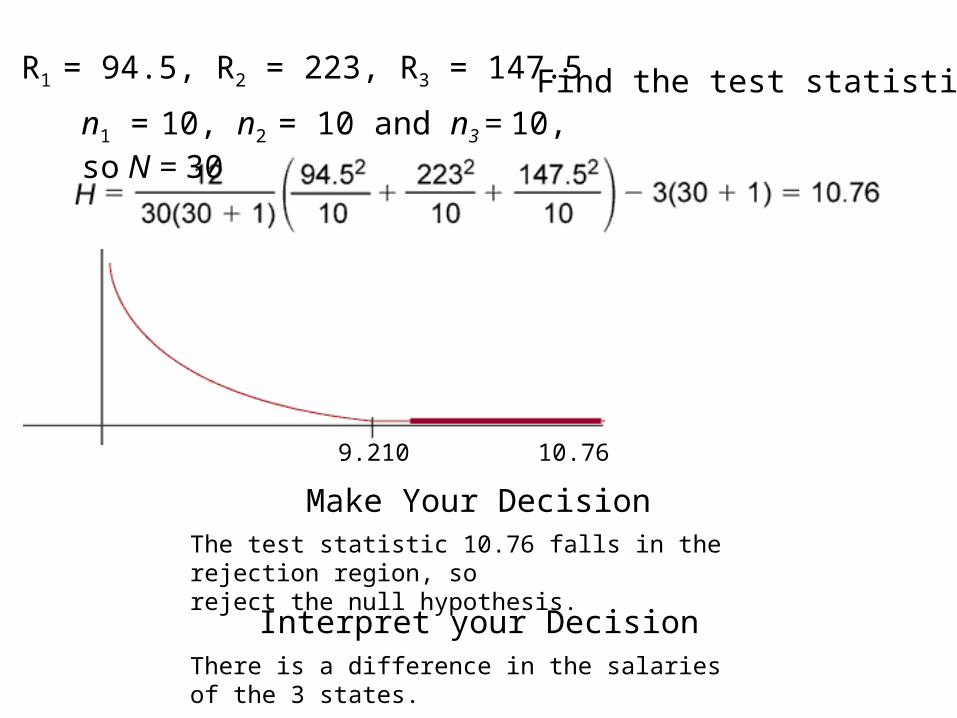
R1 = 94.5, R2 = 223, R3 = 147.5

n1 = 10, n2 = 10 and n3 = 10, so N = 30

The test statistic 10.76 falls in the rejection region, soreject the null hypothesis.

There is a difference in the salaries of the 3 states.

Find the test statistic.

Make Your Decision

Interpret your Decision

9.210 10.76

Rank Correlation

Section 11.4

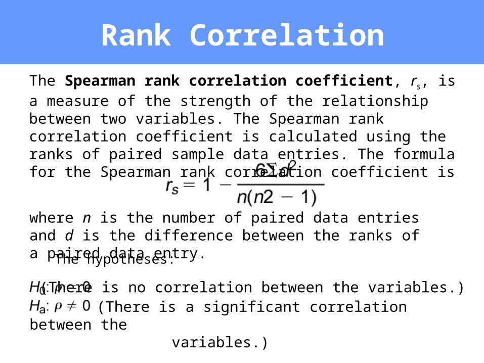
(There is a significant correlation between the variables.)

Rank CorrelationThe Spearman rank correlation coefficient, rs, is a measure of the strength of the relationship between two variables. The Spearman rank correlation coefficient is calculated using the ranks of paired sample data entries. The formula for the Spearman rank correlation coefficient is

where n is the number of paired data entries and d is the difference between the ranks of a paired data entry.

The hypotheses:

(There is no correlation between the variables.)

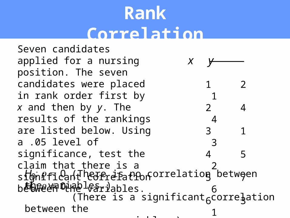
Rank CorrelationSeven candidates applied for a nursing position. The seven candidates were placed in rank order first by x and then by y. The results of the rankings are listed below. Using a .05 level of significance, test the claim that there is a significant correlation between the variables.

(There is no correlation between the variables.) (There is a significant correlation between the variables.)

x y

1 2 1 2 4 4 3 1 3 4 5 2 5 7 6 6 3 1 7 6 7

Application

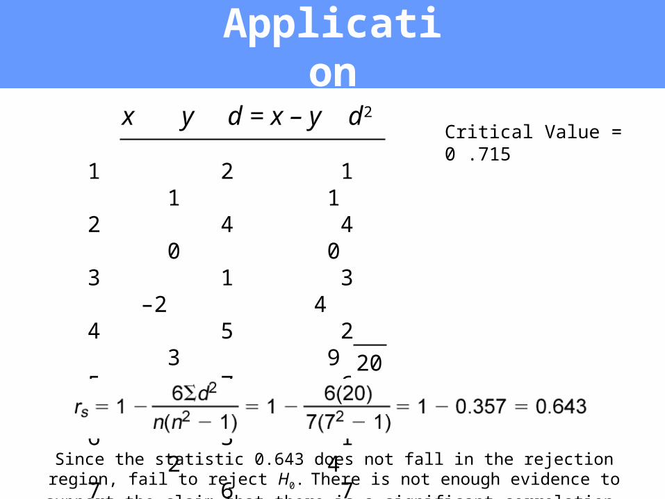
Critical Value = 0 .715

Since the statistic 0.643 does not fall in the rejection region, fail to reject H0. There is not enough evidence to support the claim that there is a significant correlation.

x y d = x – y d2

1 2 1 1 1 2 4 4 0 0 3 1 3 –2 4 4 5 2 3 9 5 7 6 1 1 6 3 1 2 4 7 6 7 –1 1 20