(NON)RANDOMIZATION: A THEORY OF QUASI-EXPERIMENTAL EVALUATION OF SCHOOL QUALITY

By

Yusuke Narita

November 2016 Revised August 2017

COWLES FOUNDATION DISCUSSION PAPER NO. 2056R

COWLES FOUNDATION FOR RESEARCH IN ECONOMICS YALE UNIVERSITY

Box 208281 New Haven, Connecticut 06520-8281

http://cowles.yale.edu/

(Non)Randomization:

A Theory of Quasi-Experimental Evaluation of School Quality

Yusuke Narita∗†

August 19, 2017

Abstract

Many centralized school admissions systems use lotteries to ration limited seats at over-

subscribed schools. The resulting random assignment is used by empirical researchers

to identify the effect of entering a school on outcomes like test scores. I first find that

the two most popular empirical research designs may not successfully extract a ran-

dom assignment of applicants to schools. When do the research designs overcome this

problem? I show the following main results for a class of data-generating mechanisms

containing those used in practice: One research design extracts a random assignment

under a mechanism if and practically only if the mechanism is strategy-proof for schools.

In contrast, the other research design does not necessarily extract a random assignment

under any mechanism.

Keywords: Matching Market Design, Natural Experiment, Program Evaluation, Ran-

dom Assignment, Quasi-Experimental Research Design, School Effectiveness

∗Yale University, Department of Economics and Cowles Foundation. Email: yusuke.narita@yale.edu†I am grateful to discussions with Atila Abdulkadiroglu, Daron Acemoglu, Nikhil Agarwal, Josh Angrist,

Nick Arnosti, Eduardo Azevedo, Ian Ball, Dirk Bergemann, Yeon-Koo Che, David Deming, Peter Hull,Michihiro Kandori, Fuhito Kojima, Parag Pathak, Debraj Ray, Jaehee Song, Jean Tirole, Chris Walters,Kohei Yata, and seminar participants at Yale, Columbia, MIT, Seoul, Tokyo, Kyoto, Osaka, and Otaru.

1

1 Introduction

The spread of choice in public education is giving more families the option to attend a

school other than their neighborhood default. As choice has proliferated, school assignment

has grown increasingly centralized and algorithmic in order to respect heterogeneous prefer-

ences and various priorities based on family background. Centralized assignment mechanisms

solve the problem of matching the demand for school seats with their limited supply by us-

ing centralized algorithms. Such mechanisms are employed in numerous school and college

admission institutions in America, Africa, Asia, and Europe. Well-designed centralized as-

signment provides a transparent way to achieve a fair and efficient school seat allocation,

while narrowing the scope for strategic behavior (Abdulkadiroglu and Sonmez, 2003).

Moreover, centralized assignment generates valuable data for empirical research on educa-

tion. In particular, when a school is oversubscribed, mechanisms often use random lotteries to

ration limited seats among applicants. This generates quasi-experimental variation in school

assignment that opens the door to a variety of impact evaluations. Researchers used such

variation to study schools in the Bay Area (Bergman, 2016), Boston (Angrist et al., 2016),

Charlotte-Mecklenburg (Hastings et al., 2009; Deming, 2011; Deming et al., 2014), Denver

(Abdulkadiroglu et al., 2017), and New York (Bloom and Unterman, 2014; Abdulkadiroglu

et al., 2014b).1

Centralized assignment mechanisms combine lotteries, preferences, and priorities into

complex stratified randomized experiments. Empirical research designs based on such mech-

anisms therefore need to condition on appropriate objects to isolate random components of

their data-generating mechanisms. Yet, the above empirical work provides only a limited

foundation for how the research designs extract a conditionally random assignment.2

This paper studies when widely-used empirical research designs successfully extract con-

ditionally random assignment of students to schools. I focus on the two most popular research

designs. These designs are applicable to any centralized mechanism that assigns students to

1See also Hastings et al. (2012). Other studies use related regression-discontinuity-style tie-breaking rulesto evaluate college majors in Norway (Kirkeboen et al., 2016) and in Chile (Hastings et al., 2013), daycare inItaly (Fort et al., 2016), privately managed public schools in Trinidad and Tobago (Beuermann et al., 2016),as well as popular selective schools in Ghana (Ajayi, 2013), Kenya (Lucas and Mbiti, 2014), Romania (Pop-Eleches and Urquiola, 2013), Trinidad and Tobago (Jackson, 2010, 2012), and the U.S. (Abdulkadiroglu etal., 2014a; Dobbie and Fryer, 2014). Narita (2015) uses lottery-based randomization to identify a structuralmodel of evolving demand for schools.

2An exception is Abdulkadiroglu et al. (2017). See the literature review at the end of this introduction forthe relationship between my paper and theirs. The other papers simply check empirical “covariate balance.”That is, they compare the treatment and control groups by baseline characteristics or covariates that arefixed at the time of treatment assignment and not used for it. If the two groups’ covariates are similar(covariates are balanced), it is interpreted as not rejecting randomization. Covariate balance is necessarybut not sufficient for randomization.

2

schools by combining: (1) applicants’ rank-ordered preferences over schools, (2) applicants’

priority statuses (e.g., walk zone) at schools, and (3) lottery numbers for breaking ties in

priority status. Each of the empirical examples above uses one of these research designs.

The first research design is what I call the first-choice research design. This design

focuses on applicants who rank a given treatment school first and are in the “marginal

priority” group at the school. The marginal priority group means a priority group where

some students are assigned to the treatment school while others are not. Within this first-

choice subsample, some applicants are assigned to the treatment school while others are not,

though all students rank the treatment school first and share the same priority. Thus it

appears that solely lottery numbers determine treatment assignment. Based on this idea,

the first-choice research design assumes that applicants are randomly assigned to or rejected

by the treatment school conditional on being in the first-choice subsample. In the first-choice

subsample, the analyst then compares the outcomes (e.g., test scores) of students who are

assigned to the treatment school against those who are not assigned. The outcome difference

between the two groups is interpreted as a causal effect of the treatment school.

Despite its intuitive construction, it turns out that the first-choice research design may not

extract a random assignment in general. That is, applicants in the first-choice subsample may

not share the same assignment probability at the treatment school.3 This motivates me to

investigate the conditions under which the first-choice design extracts a random assignment.

I provide such conditions for a class of data-generating mechanisms nesting those used in the

above empirical examples: The first-choice research design extracts a conditionally random

assignment for a mechanism if and practically only if the mechanism is strategy-proof for

schools.4

This result has important implications for applied research. It justifies the first-choice

research design for mechanisms that are known to be strategy-proof for schools, such as

the Boston (immediate acceptance) mechanism (Ergin and Sonmez, 2006). My result also

suggests that attention should be paid to the research design for other widely-used mecha-

3How can the first-choice design fail to extract a random assignment? To gain intuition, imagine thetreatment school A has only one seat, and the first-choice subsample contains two students, 1 and 2. Student1 ranks only A while 2 ranks other schools below A. When 2 has a better lottery number than 1, 1 is rejectedby A and stops applying since 1 ranks only A. When 1 has a better lottery number, 2 is rejected by A and thenapplies for other schools, potentially crowding out other students there. These crowded-out students mayapply for A, which may crowd student 1 out of A. Such chain reactions of rejections and new applicationsdilute 1’s, but not 2’s, treatment assignment probability at A. As a result, 1 and 2 may have differenttreatment assignment probabilities even though these students constitute the first-choice subsample. Thisprevents the first-choice design from extracting a random assignment. Section 3.1 provides a more preciseexample.

4The if part is exactly true. The practically-only-if part means that the first-choice design sometimes failsto extract a random assignment for any non-strategy-proof mechanisms used in the above empirical studies(but not for all possible non-strategy-proof mechanisms).

3

nisms that are not strategy-proof for schools, such as the deferred acceptance mechanism, a

mechanism used in Charlotte, and the top trading cycles mechanism.

By contrast to the above partial justification for the first-choice design, no similar suffi-

cient condition is obtainable for another popular research design. I call this alternative the

qualification instrumental variable (IV) research design. Unlike the first-choice design (try-

ing to make assignments random by focusing on a subset of students), the qualification IV

design considers all students. It then codes a supposedly random instrumental variable for

non-random assignments. The IV is based on “qualification,” i.e., whether a student’s lottery

number is better than the worst number offered a seat at the treatment school (conditional

on priority).

I find that even in the simple case with no priorities and unit school capacities, the

qualification IV research design does not necessarily extract a random assignment for any

mechanism (within my mechanism class); that is, applicants may not share the same con-

ditional probability of qualification at the treatment school. This shows a contrast between

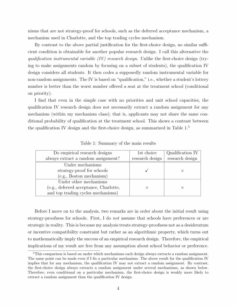
the qualification IV design and the first-choice design, as summarized in Table 1.5

Table 1: Summary of the main results

Do empirical research designs 1st choice Qualification IValways extract a random assignment? research design research design

Under mechanismsstrategy-proof for schools X ×(e.g., Boston mechanism)Under other mechanisms

(e.g., deferred acceptance, Charlotte, × ×and top trading cycles mechanisms)

Before I move on to the analysis, two remarks are in order about the initial result using

strategy-proofness for schools. First, I do not assume that schools have preferences or are

strategic in reality. This is because my analysis treats strategy-proofness not as a desideratum

or incentive compatibility constraint but rather as an algorithmic property, which turns out

to mathematically imply the success of an empirical research design. Therefore, the empirical

implications of my result are free from any assumption about school behavior or preference.

5This comparison is based on under which mechanisms each design always extracts a random assignment.The same point can be made even if I fix a particular mechanism: The above result for the qualification IVimplies that for any mechanism, the qualification IV may not extract a random assignment. By contrast,the first-choice design always extracts a random assignment under several mechanisms, as shown below.Therefore, even conditional on a particular mechanism, the first-choice design is weakly more likely toextract a random assignment than the qualification IV design.

4

In addition, I need no assumption on student behavior (e.g., truthful preference reporting). I

study whether assignment algorithms do or do not extract a random assignment conditional

on any reported preferences and without reference to true preferences. As a result, my results

do not depend on whether the reported preferences are truthful or not.

Second, the initial result — strategy-proofness for schools is sufficient for the first-choice

design to extract a random assignment — has an additional empirical implication. Par-

ticularly, it provides an asymptotic support for the first-choice design even for mechanisms

that are not strategy-proof in general. This is because such non-strategy-proof mechanisms

like deferred acceptance are known to be approximately strategy-proof for schools in certain

large markets with many students and schools (Roth and Peranson (1999) and subsequent

studies).6 This may explain why the first-choice design appears to extract a random assign-

ment in empirical applications even for non-strategy-proof mechanisms. Viewed differently,

the existing empirical justification for the first-choice design (in the form of covariate balance

regressions) may suggest the empirical relevance of theoretical results on strategy-proofness

in large markets.

The rest of this paper is organized as follows. After a literature review, the next section

introduces my model. Section 3 defines the first-choice research design and gives conditions

under which the research design extracts a random assignment. Section 4 analyzes the

alternative qualification IV design and compares it with the first-choice design. Section 5

confirms that my results are robust to a variety of modifications to the definitions of research

designs and randomization. Finally, Section 6 summarizes the empirical implications of my

theoretical results and suggests an agenda for further research.

Related Literature

This paper theoretically studies the empirical practice in econometric evaluations of school

effectiveness, such as Hastings et al. (2009); Deming (2011); Deming et al. (2014); Bloom

and Unterman (2014); Abdulkadiroglu et al. (2014b); Bergman (2016); Angrist et al. (2016).

My analysis reveals the connection between their empirical strategies and theoretical mar-

ket design studies, especially those on strategy-proofness (Ergin and Sonmez, 2006; Roth

and Peranson, 1999; Immorlica and Mahdian, 2005; Kojima and Pathak, 2009; Azevedo and

Budish, 2013; Lee, 2016; Ashlagi et al., 2016). On top of them, Abdulkadiroglu et al. (2017)

is closely related. They develop a large-sample framework based on an asymptotic approx-

imation assuming a growing number of students and school seats. They use their model

to propose an improvement over the first-choice and qualification IV designs and apply the

6See, among others, Immorlica and Mahdian (2005); Kojima and Pathak (2009); Azevedo and Budish(2013); Lee (2016); Ashlagi et al. (2016).

5

improved design to evaluate charter schools in Denver. They also confirm that the first-

choice and qualification IV designs extract a random assignment for many mechanisms in

the limit of their large market sequence. In contrast, the current paper allows for general

finite markets and provides conditions for the first-choice or qualification IV design to ex-

tract a random assignment in a finite sample. These conditions allow me to compare the

two research designs, as in Table 1. I also provide additional large market justifications for

the first-choice design in large market models different from Abdulkadiroglu et al. (2017)’s.

2 Framework

I use a model of school-student assignment with coarse school priorities and lotteries. There

are a finite set I of students and a finite set S of schools. Each student i ∈ I has a strict

preference �i over S ∪{∅}, where ∅ denotes the outside option of the student. This �i is i’s

reported preference recorded in the data; I do not make any assumption about whether �i is

truthful or not. School s is said to be acceptable for student i if s �i ∅. A preference profile

for all students is denoted by�I ≡ (�i)i∈I . Each school s has a capacity cs ∈ N where N is the

set of positive integers. Schools also grant students coarse priorities. ρis ∈ {1, ..., K} denotes

student i’s priority at school s where ρis < ρjs means s prioritizes i over j. Motivated

by public school applications, I assume every student is acceptable to every school. The

number of possible priority statuses K may change as the number of students |I| changes.Priorities may be coarse in the sense that it is possible that ρis = ρjs for some i 6= j. Let

ρs ≡ (ρis)i∈I and ρ ≡ (ρs)s∈S. Denote the type of student i by θi ≡ (�i, (ρis)s∈S). I call

X ≡ (I, S,�I , (cs)s∈S, (ρs)s∈S) an assignment problem.

2.1 Generalized Deferred Acceptance Mechanisms

A (stochastic) mechanism maps each assignment problem into a distribution over matchings

between students and schools. Mechanisms usually use lotteries to break ties in priority

and then use the resulting strict priorities to create a matching. A random variable Ris

denotes student i’s lottery number at school s. Assume that at each school, Ris is iid across

students according to U [0, 1]. For the correlation of lottery numbers across different schools,

I consider two focal regimes. Under a “single tie breaker” (STB), each student has a single

lottery number used by all schools, i.e., Ris = Ris′ always holds for all i, s, and s′. Under

a “multiple tie breaker” (MTB), each student has an independent lottery number at each

school, i.e., Ris and Ris′ are independent for all i and s 6= s′.7 Let ris ∈ [0, 1] denote

7In reality, most school districts use STB, though some cities like Washington, D.C., New Orleans, andAmsterdam use MTB. It is possible but requires messier notation to extend my analysis to any structure in

6

i’s realized lottery number at school s and let R ≡ (Ris)i∈I,s∈S, and r ≡ (ris)i∈I,s∈S. When

referring to any realized lottery number vector r, I assume no tie and ris 6= rjs for all students

i, j, and school s.

To define mechanisms of interest, I first introduce the following (student-proposing) de-

ferred acceptance (DA) algorithm (Gale and Shapley, 1962). The DA algorithm pro-

duces an assignment by using any given strict student preferences and strict school priority

orders as follows.

• Step 1: Each student i applies to her most preferred acceptable school (if any). Each

school tentatively keeps the highest-ranking students up to its capacity, and rejects

every other student.

In general, for any subsequent step t ≥ 2,

• Step t: Each student i who was not tentatively matched to any school in Step t − 1

applies to her most preferred acceptable school that has not rejected her (if any). Each

school tentatively keeps the highest-ranking students up to its capacity from the set

of students tentatively matched to this school in previous step t− 1 and the students

newly applying. The school rejects every other student.

The algorithm terminates right after the first step at which no student applies to any school.

Each student tentatively kept by a school at that step is allocated a seat in that school,

resulting in an assignment. I use this algorithm to define a class of mechanisms of interest.8

Definition 1. A generalized deferred acceptance (gDA) mechanism ϕ is a mechanism

that can be expressed as the following procedure. Take any assignment problem as given.

(1) Draw lottery numbers r according to its lottery regime (STB or MTB).

(2) For each student i and school s, compute the modified priority

ρϕis ≡ fϕ(ρis) + gϕ(rankis),

where fϕ : N → N is a strictly increasing function, gϕ : N → N is a weakly increasing

function, and rankis is the preference rank of school s in student i’s preference �i. For

example, rankis = 2 if s is i’s second choice school. Define school s’s ex post strict

modified priority order �ϕrs over students by i �ϕ

rs i′ if ρϕis + ris < ρϕi′s + ri′s.

9

between STB and MTB where some schools use a common lottery while others use independent ones.8Others also use similar classes of mechanisms. See, for example, Ergin and Sonmez (2006); Pathak and

Sonmez (2008); Agarwal and Somaini (2015); Abdulkadiroglu et al. (2017).9Note that lottery number ris is used only for tie-breaking in modified priority ρϕis since ρϕis is an integer

and ris is in (0, 1).

7

(3) Given �I and (�ϕrs)s∈S, run the DA algorithm to produce an assignment, where each

school s’s priority order is given by �ϕrs .

gDA mechanisms are parametrized by the lottery regime (STB or MTB) and the priority

modification function (fϕ, gϕ). This gDA class includes most of the mechanisms used in

empirical research as I now explain.

Deferred Acceptance Mechanism

Given an assignment problem and realized lottery numbers, the deferred acceptance (DA)

mechanism (Gale and Shapley, 1962; Abdulkadiroglu and Sonmez, 2003) makes a matching

through the DA algorithm in which schools’ strict priorities are induced by ρis + ris. The

DA mechanism makes no modification to priorities and corresponds to the gDA mechanism

with fϕ(m) = m and gϕ(n) = 0.

Boston (Immediate Acceptance) Mechanism

The Boston (immediate acceptance) mechanism (Abdulkadiroglu and Sonmez, 2003;

Ergin and Sonmez, 2006) is defined through the following immediate acceptance algorithm.

• Step 1: Each student i applies to her most preferred acceptable school (if any). Each

school accepts its highest-priority (with respect to ρis+ ris) students up to its capacity

and rejects every other student.

In general, for any step t ≥ 2,

• Step t : Each student who has not been accepted by any school applies to her most

preferred acceptable school that has not rejected her (if any). Each school accepts its

highest-priority (with respect to ρis + ris) students up to its remaining capacity and

rejects every other student.

The algorithm terminates immediately after the first step in which no student applies to

any school. Each student accepted by a school at some step of the algorithm is allocated a

seat in that school. The immediate acceptance algorithm differs from the DA algorithm in

that when a school accepts a student at a step, in the immediate acceptance algorithm, the

student is guaranteed that school, while in the deferred acceptance algorithm, that student

may be later displaced by another student with a better priority status.

The Boston mechanism can be interpreted as modifying priorities so that each school

prioritizes students ranking it higher over students ranking it lower. It is known that the

Boston mechanism is a gDA mechanism with fϕ(m) = m and gϕ(n) = (K + 1)n (Ergin and

8

Sonmez, 2006). Under this (fϕ(m), gϕ(n)), any school’s modified priority order induced by

ρϕis is lexicographic in preference ranks and priority statuses. That is, i �ϕrs i′ for all i and

i′ with rankis < ranki′s regardless of the original priorities ρis and ρi′s and lottery numbers

ris and ri′s; i �ϕrs i

′ for all i and i′ with rankis = ranki′s and ρis < ρi′s regardless of lottery

numbers ris and ri′s.

Charlotte Mechanism

The mechanism used in Charlotte is the same as the Boston mechanism except that each

school respects the walk zone priority ahead of preference ranks so that every student is

guaranteed a seat at her walk zone school (Hastings et al., 2009; Deming, 2011; Deming et al.,

2014). Assume without loss of generality that ρis = 1 means i has walk zone priority at s. The

Charlotte mechanism is a gDA mechanism with fϕ(m) = m+1{m > 1}[K +(K +1)|S|]and gϕ(n) = (K + 1)n. Under this (fϕ(m), gϕ(n)), any school’s modified priority order is

lexicographic in the walk zone priority status, preference ranks, and other (non-walk-zone)

priority statuses.10

3 First-Choice Empirical Research Design

As explained in the introduction, many empirical studies use data from gDA mechanisms

to identify and estimate the causal effect of assignment to a treatment school on outcomes

such as test scores, crime rates, college attendance, and earnings.11 Their empirical research

designs fall into two categories. I start with analyzing one of them and move on to the other

in Section 4.

To describe the first empirical strategy, fix any gDA mechanism ϕ and assignment prob-

lem X that generates the data at hand. Following the standard notation in econometrics, let

Dis(r) = 1 if student i is assigned the treatment school s under (realized or counterfactual)

lottery number profile r; Dis(r) = 0 otherwise. I consider the set of students who rank s

first and are in s’s “marginal priority group,” where some students are assigned s but others

10That is, i �ϕrs i′ for all i and i′ with ρis = 1 and ρi′s > 1; i �ϕ

rs i′ for all i and i′ with 1{ρis = 1} =1{ρi′s = 1} and rankis < ranki′s; i �ϕ

rs i′ for all i and i′ with 1{ρis = 1} = 1{ρi′s = 1}, rankis = ranki′s,and ρis < ρi′s.

11Many of the studies mentioned in the introduction investigate the effect of a group of schools ratherthan an individual school. My analysis extends to such group-level treatments too. Also, when the effectof interest is that of attendance or enrollment rather than assignment, the analyst would see attendanceor enrollment as the endogenous treatment and use assignment as an instrument for the treatment. Theanalyst would then use an instrumental variable method to estimate the effect of attendance or enrollment.My analysis is applicable to such instrumental variable settings. See footnote 15.

9

are not though all of them share the same priority at s. That is, define

Firsts(r)

≡ {i ∈ I|rankis = 1 and ∃i′ such that ranki′s = 1, ρis = ρi′s, and Dis(r) 6= Di′s(r)}.12

Let r0 be the realized profile of lottery numbers in the data.

The first widespread empirical strategy, which I call the first-choice research design,

compares the outcomes of students with Dis(r0) = 1 against those with Dis(r0) = 0 within

Firsts(r0).13 The outcome difference between the two groups is then interpreted as the

causal effect of being assigned to school s for students in Firsts(r0). The idea is that since

all students in Firsts(r0) rank s first and share the same priority at s, whether they get an

offer from s should be determined solely by their lottery numbers and hence independent of

students’ covariates or choices potentially correlated with outcomes. Therefore, offers from

s within Firsts(r0) are thought of as being randomly assigned in a randomized controlled

trial.

Albeit intuitive, for the first-choice research design to identify a causal effect by this

logic, assignments to s within Firsts(r0) have to be indeed random and not confounded

by non-random preferences or priorities. This requirement is formalized as the following

concept.

Definition 2. The first-choice research design extracts a random assignment for

a gDA mechanism ϕ if for any assignment problem X, any school s, any potential lottery

realization r, and any students j, k ∈ Firsts(r),

P (Djs(R) = 1) = P (Dks(R) = 1).

An equivalent requirement is

P (Dis(R) = 1|i ∈ Firsts(r), θi = θ) = P (Dis(R) = 1|i ∈ Firsts(r)),

12Since rankis = ranki′s = 1 holds and fϕ(·) is strictly increasing by definition, ρis = ρi′s is equivalent to

(fϕ(ρis) + gϕ(1) ≡)ρϕis = ρϕi′s(≡ fϕ(ρi′s) + gϕ(1)).

I could therefore replace ρis = ρi′s with ρϕis = ρϕi′s in the definition of Firsts(r) without changing anythingin the following analysis. Note also that it is possible Firsts(r) = ∅ for some or even all r.

13Applications of the first-choice research design include Hastings et al. (2009); Deming (2011); Deming etal. (2014); Abdulkadiroglu et al. (2014b); Bloom and Unterman (2014); Angrist et al. (2016). The first threestudies use data from the Charlotte mechanism while the remaining studies are based on the DA mechanism.

10

for any student type θ for which the left-hand-side conditional probability is well-defined.

P (Dis(R) = 1|i ∈ Firsts(r), θi = θ) means the probability of assignment to s for an arbitrary

student of type θ in Firsts(r).

This property requires that conditional on being in Firsts(r0), offers from s are random and

independent of students’ preferences and priorities summarized by θi. In the econometric

terminology, this requires that the propensity score (Rosenbaum and Rubin, 1983) is con-

stant across all students in Firsts(r0).14 Only under this conditionally random assignment

are the treatment and control groups in Firsts(r0) comparable with each other. Economet-

ric program evaluation methods require this conditional independence for the first-choice

research design to identify a causal treatment effect (Heckman and Vytlacil (2007) chapters

8 and 9, Manski (2008) chapters 3 and 7, Angrist and Pischke (2009) chapter 3.2).15

3.1 Motivating Example

While the first-choice research design is intuitive, this design may fail to extract a random

assignment. Consider the following example.

Example 1. There are applicants 1, 2, 3, and schools A and B with the following prefer-

ences and priorities:

�1 : A,B, ∅�2 : A, ∅�3 : B,A, ∅ρA : 3, {1, 2}ρB : 1, {2, 3},

where �1: A,B, ∅ means 1 prefers A over B and both schools are acceptable for 1. ρA :

3, {1, 2} means that A prioritizes 3 over 1 and 2 and is indifferent between 1 and 2. The

capacity of each school is 1. The treatment school is A.

14It is possible to define random assignment conditional on being in random Firsts(R), where R arerandom lottery numbers and Firsts(R) is a random set. Alternatively, it is also reasonable to define randomassignment as that all students who rank school s first and who have the same priorities at school s sharethe same assignment probability at s. My result is robust to using such alternative definitions; see Section5.1 for more discussions.

15When assignment within Firsts(r0) is used as an instrument for an endogenous treatment such asenrollment, Definition 2 is interpreted as a conditional independence requirement for the instrument. Forthe instrument to identify a causal effect, it usually needs to additionally satisfy properties such as “exclusion”or “monotonicity.” See Heckman and Vytlacil (2007); Manski (2008); Angrist and Pischke (2009). In thiscase, Definition 2 becomes a necessary condition for legitimate causal inference. See also Sections 4 and 5.2for related discussions.

11

In this example, the first-choice research design does not extract a random assignment

for A for the DA mechanism (with no priority modification). Under the DA mechanism, 1

is assigned to A when 1 has a better lottery number than 2 at A. Otherwise, 3 is assigned

to A. Each of the two cases occurs with equal probability 0.5. Thus,

P (D1A(R) = 1) = 0.5 6= 0 = P (D2A(R) = 1),

despite

FirstA(r) =

{1, 2} if r1A < r2A

∅ otherwise.

Therefore, the first-choice research design does not extract a random assignment for the DA

mechanism.

It is possible to create a similar counterexample even when there are no priorities (as long

as ties are broken by MTB). Also, the first-choice research design may fail even if I modify

it to the more conditional version that pools applicants who rank the treatment school first

and share the same priority at every school. Finally, the problem with the first-choice design

does not depend on short preferences; the problem turns out to persist even if I require every

student to rank all schools. I explain these points in Section 5.2.

The above problem may bias treatment effect estimates. Imagine that school A has

no real treatment effect, and student 1 ranks more schools than student 2 because student

1 is more eager and higher achieving (regardless of whether she attends A). Whenever

FirstA(r) = {1, 2}, student 1 gets the seat at A and student 2 does not. Comparing 1 and

2 within FirstA(r) = {1, 2}, the researcher is likely to mistakenly conclude A has a positive

achievement effect.

Such a correlation between preferences and outcomes is empirically observed in data from

Denver Public Schools. Denver Public Schools use the DA mechanism for unified public

and charter school admissions (Abdulkadiroglu et al., 2017). Each year more than 10000

applicants in grades 4-10 participate in this system. These applicants are predominantly

black and hispanic and from needy households. I use Denver’s data for school years 2011-

2013 to correlate applicant preference lengths and pre-application baseline test scores, which

are likely to be predictive of potential outcomes after mechanism participation.

There turns out to be a clear correlation between preference length and baseline scores,

as seen in Table 2. For all of math, reading, and writing, students with higher baseline

scores tend to rank more schools; there is about 0.15 standard deviation score difference

between students who rank only one school and those who rank two or more schools. This

12

is reasonable if, for example, higher-achieving students are more willing to investigate and

rank schools because of smaller learning costs. This empirically suggests that student type

is correlated with potential outcomes and is a source of potential omitted variable bias, as

the above theoretical story assumes.

Table 2: Empirical Correlation between Preferences and Outcomes

Notes: This table shows average baseline test scores for students who rank different numbers of schools.Each test score is standardized to the test score distribution for the whole population of students in DenverPublic Schools.

The above example raises the question: Under what circumstances does the first-choice

research design extract a random assignment as desired?

3.2 Strategy-proofness for Schools

The success or failure of the first-choice research design turns out to be linked to a seemingly

unrelated property of mechanisms. So far, I have treated priorities and lottery numbers as

public information. In this section, I depart from this assumption and imagine a hypothetical

situation in which schools have priorities and lottery numbers as their private information.

The priorities and lottery numbers are assumed to represent school preferences; I come

back to the interpretation of this thought experiment at the end of this section. Suppose

a gDA mechanism asks schools to report priorities and lottery numbers. Their reports are

not necessarily truthful. The gDA mechanism then uses the reported priorities and lottery

numbers to create a matching.

Given any (I, S,�I , (cs)s∈S), let Γ ≡ {(ρs, rs) ∈ {1, ..., K}|I| × [0, 1]|I||ρis + ris 6= ρjs +

rjs for all students i 6= j} be the domain of possible priority and lottery number reports.

This domain specification implies every student is acceptable to every school in any reported

priority and lottery numbers. A gDA mechanism asks each school s to report its priority and

lottery numbers (ρs, rs), producing (ρ, r) ≡ (ρs, rs)s∈S. Let ϕ(ρ, r) ≡ (ϕs(ρ, r))s∈S be the

assignment produced by a gDA mechanism ϕ for the reported priority and lottery numbers

(ρ, r).

School s’s preference �s, which is defined over the set of subsets of I, is said to be

responsive with respect to (cs, ρs, rs) (Roth and Sotomayor, 1992) if the following holds.

13

(1) For any i, i′ ∈ I, if ρis+ris < ρi′s+ri′s, then for any I ′ ⊆ Ir{i, i′}, I ′∪{i} �s I′∪{i′},

(2) ∅ �s I′ for any I ′ ⊆ I with |I ′| > cs, and

(3) For any I ′ ⊆ I with |I ′| < cs and any i ∈ I \ I ′, it holds I ′ ∪ {i} �s I′.

I use these concepts to define the following property.

Definition 3. A gDA mechanism ϕ is strategy-proof for school s if for any (I, S,�I

, (cs)s∈S), any priority and lottery number profile (ρ∗, r∗) ∈ Γ|S|, any preference �∗s responsive

with respect to (cs, ρ∗s, r

∗s), and any (ρ′s, r

′s) ∈ Γ,

ϕs(ρ∗, r∗) �∗

s ϕs((ρ′s, r

′s), (ρ

∗−s, r

∗−s)),

where �∗s is the weak preference associated with �∗

s and (ρ∗−s, r∗−s) ≡ (ρ∗s′ , r

∗s′)s′ 6=s. A gDA

mechanism ϕ is strategy-proof for schools if it is strategy-proof for every school s.

This definition of strategy-proofness is a non-stochastic, ex post property though my setting

has stochastic elements due to lotteries. The standard behavioral interpretation of this

concept is that no school ever has a preference manipulation that is profitable with respect

to its true preference. It is crucial to note, however, that I am not concerned with this usual

interpretation. As will become clearer in the next section, unlike usual studies on strategy-

proofness, I am interested only in the mathematical implications of strategy-proofness for

empirical research. These implications are true regardless of whether strategy-proofness

itself has any relevance as an incentive compatibility property or desideratum. As a result,

the following usual questions about strategy-proofness for schools are all irrelevant for my

analysis: Do schools have preferences? Are school preferences consistent with priorities? Do

schools ever game the system?

3.3 Sufficiency: Strategy-proofness Generates Natural Experiments

Strategy-proofness for schools turns out to be sufficient for the first-choice research design

to extract a random assignment.

Theorem 1. The first-choice research design extracts a random assignment for a gDA mech-

anism ϕ if ϕ is strategy-proof for schools.

The proof is in Appendix A.1. Combined with existing results on strategy-proofness for

schools, Theorem 1 provides positive results for the first-choice research design for some of

the gDA mechanisms.

14

Corollary 1. a) The first-choice research design extracts a random assignment for the

Boston mechanism with any lottery regime.

b) The first-choice research design extracts a random assignment for the DA mechanism

with STB when there are no priorities (ρis = ρjs for all students i, j and school s). This

mechanism is often called random serial dictatorship.

Proof. (a) follows from Theorem 1 and Ergin and Sonmez (2006)’s Theorem 2 that the

Boston mechanism is strategy-proof for schools. (b) follows from the proof of Theorem 1

and the fact that for the DA mechanism, truth-telling is optimal for any school s when all

the other schools report the same preference as s’s true preference. See Appendix A.2 for

details.

I illustrate Theorem 1 with the Boston mechanism. Consider Example 1 in Section 3.1

and a thought experiment where schools have private preferences and the mechanism asks

schools to report their preferences. First of all, school A is never matched with student 3

since 3 ranks A second and the seat at A is always filled by one of the two students who

rank A first. A is thus matched with either 1 or 2. When A’s true preference is such that

1 �A 2, A is matched with the more preferred student 1 by truth-telling.16 When A’s true

preference is with 2 �A 1, A is matched with the more preferred student 2 by truth-telling.

Therefore, there is no profitable preference manipulation for A; the Boston mechanism is

strategy-proof for A in Example 1 (Ergin and Sonmez, 2006).

As it should be by strategy-proofness and Theorem 1, the first-choice research design

extracts a random assignment for A in Example 1 for the Boston mechanism. Note that

FirstA(r) = {1, 2} for all r since only 1 and 2 rank A first with the same priority and

only one of them with a better lottery number is assigned A under any r. Enumerating all

lottery outcomes shows that 1 and 2 share the same assignment probability of 1/2 at A, i.e.,

P (D1A(R) = 1) = P (D2A(R) = 1) = 1/2. Therefore the first-choice research design extracts

a random assignment.

Illustrative Proof of a Special Case of Theorem 1

Readers who are not interested in the proof may skip the remainder of this section and jump

to Section 3.4. The full proof of Theorem 1 is long and involved. For purposes of illustration,

this section provides a simpler proof for a special case of Theorem 1. The special case of

interest is formulated as follows.

16Since A’s capacity is 1, I do not need to distinguish its preference over sets of students and its priorityorder over individual students.

15

Corollary 2. Consider assignment problems with no priorities (ρis = ρjs for all students i

and j and school s) and unit school capacities (cs = 1 for all s). The first-choice research

design extracts a random assignment for a gDA mechanism ϕ with a multiple tie breaker

(MTB) if ϕ is strategy-proof for schools.

A formal proof of this fact needs a few definitions. Given any gDA mechanism ϕ and

lottery number profile r, I say two students i0 and i1 are consecutive in rs within Firsts(r)

if i0, i1 ∈ Firsts(r) and there is no other student j ∈ Firsts(r) such that ri0s < rjs < ri1s

or ri0s > rjs > ri1s. As per usual, a permutation of rs is a bijection from {ris}i∈I to

{ris}i∈I itself. A permutation r′s of rs is said to be a first-choice transposition of rs at

r if r′s switches only two students i0 and i1 who are consecutive in rs within Firsts(r), i.e.,

r′i0s = ri1s, r′i1s

= ri0s, and r′js = rjs for all j 6= i0, i1. I use these definitions to introduce a

key property of mechanisms.

Definition 4. Suppose that the assumptions in Corollary 2 hold. I say a gDA mechanism ϕ

with MTB satisfies the Fisher property if given ϕ, for any (I, S,�I), any school s, any

lottery number profile r and any first-choice transposition r′s of rs at r that switches only

two students i0 and i1, the following is true:

• Di1s(r′s, r−s) = Di0s(r),

• Di0s(r′s, r−s) = Di1s(r), and

• Djs(r′s, r−s) = Djs(r) for all j 6= i0, i1.

In words, a gDA mechanism with MTB satisfies the Fisher property if for that mechanism,

any transposition of lottery numbers within the first-choice subsample translates into the

same transposition of assignments. Since any permutation is a combination of transpositions,

the Fisher property implies that any permutation of lottery numbers in the first-choice

subsample always induces the same permutation of assignments. I name this the Fisher

property after Ronald Fisher (the inventor of randomized experiments) since this property

is reminiscent of a randomized controlled trial, where random numbers pin down treatment

assignment. Note that the Fisher property implies that for any (I, S,�I), any school s, any

lottery number profile r and any first-choice transposition r′s of rs at r,

Firsts(r) = Firsts(r′s, r−s). (1)

Not surprisingly, I find that if a gDA mechanism with MTB satisfies the Fisher prop-

erty, then the first-choice research design extracts a random assignment for that mechanism.

16

Moreover, less trivially, strategy-proofness for schools turns out to imply the Fisher property,

showing Corollary 2. I prove these facts in the following proof of Corollary 2.

Proof of Corollary 2. The proof consists of two steps, Lemmas 1 and 2 below.

Lemma 1. Under the assumptions in Corollary 2, the first-choice research design extracts

a random assignment for a gDA mechanism ϕ with MTB if ϕ satisfies the Fisher property.

Proof of Lemma 1. Consider any assignment problem X and let R ≡ {r ∈ [0, 1]|I|×|S||ris 6=rjs for all students i, j, and school s} be the set of all possible values of the lottery number

profile r. Fix any gDA mechanism ϕ with MTB and the Fisher property, any school s, and

any potential lottery realization r. Partition R into P ≡ {Rn}n∈N (N is an uncountable set

of indices) such that the following holds: Within each Rn, any r′ ∈ Rn can be obtained from

any other r′′ ∈ Rn by applying a finite number of first-choice transpositions at school s, i.e.,

there exists a sequence of lottery number profiles (r1, r2, ..., rK) such that r1 = r′′, rK = r′,

and for each k = 2, ..., K, rks is a first-choice transposition of rk−1s at rk−1.17

The Fisher property and equation (1) imply that conditional on each Rn, Firsts(rn) and

os(rn) ≡ |{i ∈ Firsts(rn)|Dis(rn) = 1}| are constant for all rn ∈ Rn. This means that for

each rn ∈ Rn, students with the os(rn)-best lottery numbers in Firsts(rn) have Dis(rn) = 1,

which happens with probabilityos(rn)

|Firsts(rn)|for any i ∈ Firsts(rn) conditional on Rn. Also,

whenever Firsts(rn) and Firsts(r) are nonempty, Firsts(r) = Firsts(rn) = {i|rankis = 1}by the no-priority assumption. Therefore, for each n ∈ N ,

P (Dis(R) = 1|i ∈ Firsts(r), R ∈ Rn, θi = θ)

=

os(rn)

|Firsts(rn)|if Firsts(rn) 6= ∅

1 if Firsts(rn) = ∅ and Djs(rn) = 1 for all rn and all j ∈ Firsts(r)

0 if Firsts(rn) = ∅ and Djs(rn) = 0 for all rn and all j ∈ Firsts(r)≡ pn,

which is independent of θi.18

17This partition is well-defined since the assumption that ϕ satisfies the Fisher property guarantees equa-tion (1), which in turn implies that r′ can be obtained from r′′ with a finite number of first-choice transposi-tions if and only if r′′ can be obtained from r′ with a finite number of first-choice transpositions. Note alsothat this partition depends on particular school s I focus on.

18In the above definition of pn, the three cases are exhaustive by the following reason. WheneverFirsts(rn) = ∅, it has to be the case that Rn = {rn} (i.e., Rn is a singleton) since there is no first-choice transposition of rns with Firsts(rn) = ∅. For the single element rn, there are only two possibilities,(i) Djs(rn) = 1 for all j ∈ Firsts(r) or (ii) Djs(rn) = 0 for all j ∈ Firsts(r). To see this, suppose to the

17

Let Y be Y (R) = RRn where RR

n is the element of the partition P with R ∈ RRn . Let PY

be the probability measure of Y induced by that of R, i.e. for all A ⊂ N , PY ({Rn}n∈A) ≡P (R ∈ ∪n∈ARn). With this notation, I have

P (Dis(R) = 1|i ∈ Firsts(r), θi = θ)

=

∫{Rn}n∈N

P (Dis(R) = 1|i ∈ Firsts(r), Y = Rn, θi = θ)dPY (Rn)

(by the law of iterated expectation)

=

∫{Rn}n∈N

pndPY (Rn),

which is again independent of θi since both pn and PY are independent of θi. Thus P (Dis(R) =

1|i ∈ Firsts(r), θi = θ) = P (Dis(R) = 1|i ∈ Firsts(r)), and the first-choice research design

extracts a random assignment. This completes the proof of Lemma 1.

Lemma 2. Under the assumptions in Corollary 2, a gDA mechanism ϕ with MTB satisfies

the Fisher property if ϕ is strategy-proof for schools.

Proof of Lemma 2. As in Definition 4 of the Fisher property, consider any gDA mechanism

ϕ with MTB, any (I, S,�I), any school s, any lottery number profile r, and any first-choice

transposition r′s of rs at r that switches only two students i0 and i1. Assume that ϕ is

strategy-proof for schools. Without loss of generality, assume ri1s < ri0s, i.e, student i1 has

a better original lottery number than i0 at school s. This assumption makes it impossible

that Di0s(r) = 1 and Di1s(r) = 0 since i0, i1 ∈ Firsts(r) and so ρϕi0s = ρϕi1s and both i0 and

i1 rank s first. Di0s(r) = Di1s(r) = 1 is also impossible by the unit capacity assumption of

cs = 1. There are two remaining cases, Cases i and ii below.

Case i : Di0s(r) = 0 and Di1s(r) = 1, i.e., i1 is assigned to s while i0 is not under r. To

reach the desired Fisher property, consider the DA algorithm inside the gDA mechanism with

(r′s, r−s). In the first round of the DA algorithm, students i0 and i1 apply to school s (as it is

their first choice by i0, i1 ∈ Firsts(r)). School s’s single seat is tentatively assigned to i0; it is

because (a) Di1s(r) = 1 and so student i1 is tentatively assigned to school s in the first round

of the DA algorithm under r, (b) the same set of applicants apply to school s in the first round

of the DA algorithm with (r′s, r−s) and r, and (c) ρϕi0s+r′i0s = ρϕi1s+ri1s < ρϕi1s+r′i1s = ρϕi0s+ri0s

while ρϕjs + r′js = ρϕjs + rjs for all j 6= i0, i1. The tentative assignment of i0 to s will never be

canceled, as I claim below.

contrary that there are j, k ∈ Firsts(r) such that Djs(rn) 6= Dks(rn). Then j and k must be in Firsts(rn)by the definition of the first-choice subsample. But this is a contradiction to Firsts(rn) = ∅.

18

Claim 1. Di0s(r′s, r−s) = 1, i.e., school s’s single seat is assigned to i0 at the end of the DA

algorithm with (r′s, r−s).

Proof of Claim 1. Suppose not. In second or later rounds of the DA algorithm with (r′s, r−s),

school s must reject i0 in favor of some student j( 6= i0, i1) with better lottery number

r′js < r′i0s. This implies by the construction of first-choice transposition r′s that rjs = r′js <

r′i0s = ri1s. In other words,

{j} �s {i1} (2)

for any preference �s responsive with respect to (cs, ρs, rs) where cs = 1 and ρis = ρks for

all students i and k as required by the assumptions in Corollary 2.

The definition of the DA algorithm with (r′s, r−s) ensures that the tentatively assigned

student at s improves with respect to r′s and so with respect to any preference �′s re-

sponsive with respect to (cs, ρs, r′s). For any such preference �′

s, therefore, it is the case

that ϕs(r′s, r−s) �′

s {j}. This implies that for any preference �s responsive with respect to

(cs, ρs, rs),

ϕs(r′s, r−s) �s {j}. (3)

This is because (a) k 6= i0, i1 for student k defined by {k} = ϕs(r′s, r−s) and (b) by the

construction of r′s, for any students j, h 6= i0, i1, I have rhs < rjs if and only if r′hs < r′js.

Combining these steps (2), (3), and Di1s(r) = 1 together, for any preference �s responsive

with respect to (cs, ρs, rs), I have

ϕs(r′s, r−s) �s {j} �s {i1} = ϕs(r). (4)

However, the preference relation (4) contradicts the assumption that ϕ is strategy-proof for

schools. Therefore, student i0 will be assigned to school s, proving Claim 1.

This Claim, cs = 1, and the assumption of Di0s(r) = 0 and Di1s(r) = 1 jointly imply that

• Di1s(r′s, r−s) = Di0s(r) = 0,

• Di0s(r′s, r−s) = Di1s(r) = 1, and

• Djs(r′s, r−s) = Djs(r) = 0 for all j 6= i0, i1,

proving the Fisher property for Case i.

19

Case ii : Di0s(r) = Di1s(r) = 0, i.e., neither i0 nor i1 is assigned to s at r. This means

that for any preference �s responsive with respect to (cs, ρs, rs) (with cs = 1 and ρis = ρks

for all students i and k), I have

ϕs(r) �s {i0} and ϕs(r) �s {i1}, (5)

since school s tentatively keeps a student while rejecting i0 and i1, both of whom are

in Firsts(r) and apply for s at the first step of the DA algorithm with r. To show

the Fisher property, suppose to the contrary that the Fisher property does not hold, i.e.,

Di1s(r′s, r−s) 6= Di0s(r) or Di0s(r

′s, r−s) 6= Di1s(r) or Djs(r

′s, r−s) 6= Djs(r) for some j 6= i0, i1.

There are two sub-cases to discuss.

Case ii.a: Di1s(r′s, r−s) 6= Di0s(r) = 0 or Di0s(r

′s, r−s) 6= Di1s(r) = 0. This requires

Di0s(r′s, r−s) = 1 and Di1s(r

′s, r−s) = 0 by the assumption of r′i0s = ri1s < ri0s = r′i1s and

the unit capacity assumption of cs = 1. Equivalently, ϕs(r′s, r−s) = {i0}. Together with

the preference relation (5), it has to be the case that for any preference �′s responsive with

respect to (cs, ρs, r′s), I have

({k} ≡)ϕs(r) �′s {i0} = ϕs(r

′s, r−s). (6)

or, equivalently, r′ks < r′i0s. This is because student k has rks < ri0s, ri1s by the preference

relation (5) and the construction of r′s guarantees r′ks < r′i0s, r′i1s. However, the preference

relation (6) contradicts the assumption that ϕ is strategy-proof for schools. Therefore, the

Fisher property must hold for Case ii.a.

Case ii.b: Di1s(r′s, r−s) = Di0s(r) = 0 and Di0s(r

′s, r−s) = Di1s(r) = 0, but Djs(r

′s, r−s) 6=

Djs(r) for some j 6= i0, i1. This implies ϕs(r′s, r−s) 6= ϕs(r) while i0, i1 6∈ ϕs(r

′s, r−s) ∪ ϕs(r).

The construction of r′s implies that for any preferences �s and �′s responsive with respect

to (cs, ρs, rs) and (cs, ρs, r′s), respectively, I have

[ϕs(r′s, r−s) �s ϕs(r) and ϕs(r

′s, r−s) �′

s ϕs(r)] (7)

or

[ϕs(r) �s ϕs(r′s, r−s) and ϕs(r) �′

s ϕs(r′s, r−s)]. (8)

Both (7) and (8) contradict the assumption that ϕ is strategy-proof for schools. Thus the

Fisher property must hold, completing the proof of Lemma 2.

20

Lemmas 1 and 2 jointly prove Corollary 2.

This proof of Corollary 2 is still far from a complete proof of Theorem 1, however. For

instance, Theorem 1 allows additional complications like priorities, non-unit capacities, and

STB, all of which the above proof ignores. Nevertheless, the proof in Appendix A.1 shows

that the sufficiency of strategy-proofness generally holds.

3.4 Necessity in Practice

Theorem 1 shows that strategy-proofness for schools is sufficient for the first-choice research

design to extract a random assignment. Strategy-proofness turns out to be not only sufficient

but also necessary as long as I focus on practically important mechanisms.

Proposition 1. Even with unit school capacities (cs = 1 for all s), the first-choice research

design does not extract a random assignment for the DA, Charlotte, and “top trading cycles”

mechanisms (with any lottery regime), all of which are known to be not strategy-proof for

schools.

To illustrate this, consider the DA mechanism in Example 1. Imagine A’s true preference

is 3 �A 1 �A 2 while B’s is 1 �B 2 �B 3. Under these true preferences, A is matched with

1. If A misreports 3 �′A 2 �′

A 1, however, A is matched with 3, the most preferred student

with respect to �A. Therefore, the DA mechanism is not strategy-proof for A in Example

1. This confirms the classic result that the DA mechanism is not strategy-proof for schools

(Roth and Sotomayor, 1992).

Intuitively, school A benefits from manipulating its preference and rejecting 1 by the

following chain reaction of rejections and new applications. After being rejected by A,

student 1 next applies for B, which results in B’s rejecting 3. Student 3, the most preferred

student for A, then applies for and benefits A.

The same chain reaction causes the first-choice research design to fail, as I explain in

Section 3.1. Different applicants cause different chain reactions that have different effects

on assignment probabilities at A, depending on schools ranked below A. This can cause

applicants in FirstA(r0) to have different assignment probabilities at A.19

19In contrast, for the Boston mechanism analyzed in the last section, such chain reactions do not affectassignments to A. By its construction, for the Boston mechanism, each school is forced to prioritize studentsranking it higher over students ranking it lower. As a result, chain reactions caused by student i at schoolsranked below A involve only students who rank A lower than student i does. Any such student in chainreactions i causes is never accepted by A since A rejects i. Thus, different chain reactions caused by differentstudents have no effect on assignments at A. This is the reason why the Boston mechanism is strategy-prooffor schools and the first-choice research design extracts a random assignment for the Boston mechanism.

21

Similarly, the first-choice research design does not extract a random assignment for the

Charlotte mechanism, another mechanism that is not strategy-proof for schools. Suppose

that in Example 1, student 3’s priority at A and 1’s priority at B are walk zone priorities.

In this case, the Charlotte mechanism coincides with the DA mechanism. The Charlotte

mechanism is therefore manipulable by schools and the first-choice research design fails in

the same way as for the DA mechanism. Section 5.3 also shows the same failure of the

first-choice design for the top trading cycles mechanism, which is not strategy-proof for

schools either. In these senses, for mechanisms frequently discussed in theory and practice,

strategy-proofness for schools is required for the first-choice research design to extract a

random assignment.20 The analyst therefore needs to take care when using the first-choice

design for non-strategy-proof mechanisms such as the DA, Charlotte, and top trading cycles

mechanisms.

Empirical Illustration

The DA mechanism is not strategy-proof for schools and may not extract a random assign-

ment via the first-choice design. To see whether the theoretical result has any relevance in

practice, I use data from Denver Public Schools, which use the usual DA mechanism with

STB for unified public and charter school admissions (Abdulkadiroglu et al., 2017). I use its

DA mechanism in school years 2011-2012 as follows.

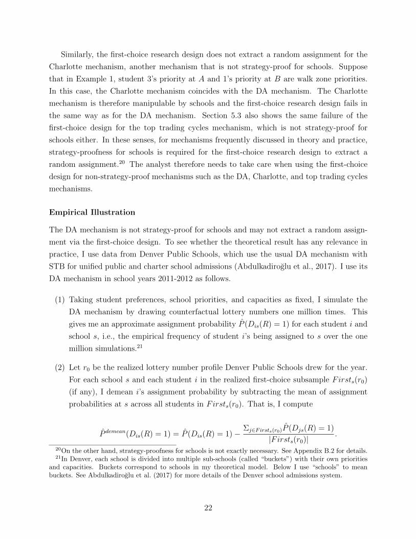
(1) Taking student preferences, school priorities, and capacities as fixed, I simulate the

DA mechanism by drawing counterfactual lottery numbers one million times. This

gives me an approximate assignment probability P (Dis(R) = 1) for each student i and

school s, i.e., the empirical frequency of student i’s being assigned to s over the one

million simulations.21

(2) Let r0 be the realized lottery number profile Denver Public Schools drew for the year.

For each school s and each student i in the realized first-choice subsample Firsts(r0)

(if any), I demean i’s assignment probability by subtracting the mean of assignment

probabilities at s across all students in Firsts(r0). That is, I compute

P demean(Dis(R) = 1) = P (Dis(R) = 1)−Σj∈Firsts(r0)P (Djs(R) = 1)

|Firsts(r0)|.

20On the other hand, strategy-proofness for schools is not exactly necessary. See Appendix B.2 for details.21In Denver, each school is divided into multiple sub-schools (called “buckets”) with their own priorities

and capacities. Buckets correspond to schools in my theoretical model. Below I use “schools” to meanbuckets. See Abdulkadiroglu et al. (2017) for more details of the Denver school admissions system.

22

(3) I plot this assignment probability deviation P demean(Dis(R) = 1) across all schools s

and all students in Firsts(r0).

Figure 1: Empirical Illustration of Proposition 1

020

040

060

080

010

00Fr

eque

ncy

-1 -.5 0 .5 1(Propensity Score at 1st Choice School)-(Mean at Each School)

The resulting histogram of assignment probability deviations is in Figure 1. If the 1st

choice method extracts a random assignment, P (Dis(R) = 1) ≈ P (Djs(R) = 1) for all s and

all i, j ∈ Firsts(r0) and so the assignment probability deviation P demean(Dis(R) = 1) would

be almost 0 (up to simulation errors) for all s and all i in Firsts(r0). As the figure shows,

however, there are many values of P demean(Dis(R) = 1) that are far from 0. The standard

deviation is around 0.19. This provides an empirical illustration of the theoretical necessity

of strategy-proofness for schools.

4 Qualification Instrumental Variable Research Design

While the previous sections focus on the first-choice research design, several empirical studies

use an alternative research design. I call this alternative the qualification instrumental

variable (IV) research design.22 Unlike the first-choice research design (which tries to make

assignments random by focusing on a subset of students), the qualification IV research design

considers all students and tries to code a random instrumental variable for non-random

assignments. Define the qualification IV by

22For empirical examples of the qualification IV design, see Pop-Eleches and Urquiola (2013); Dobbie andFryer (2014); Lucas and Mbiti (2014), all of which use data from the DA mechanism.

23

Zis(r) ≡ 1{ρϕis + ris ≤ max{ρϕjs + rjs|Djs(r) = 1}}.

If there is no student j with Djs(r) = 1, then define Zis(r) = 1 for all i. The qualification

IV for a student at a school is turned on if her realized priority rank at the school is better

than that of some student assigned to the school. Note that Zis(r) = 1 is possible even for

students who do not apply to school s.

The qualification IV looks unconfounded conditional on ρϕis. The IV is also likely to be

correlated with assignmentDis(r) since i can get assigned only when she is qualified (Zis(r) =

1). Based on this idea, the qualification IV research design instruments for assignment

Dis(r) by qualification Zis(r) conditional on ρϕis. The design then estimates treatment effects

by Two Stage Least Square or other instrumental variable models (Heckman and Vytlacil

(2007) chapter 4, Manski (2008) chapter 3, Angrist and Pischke (2009) chapter 4).23 For this

research design to identify a causal effect, the qualification IV needs to be random conditional

on ρϕis, as formalized in the following definition.

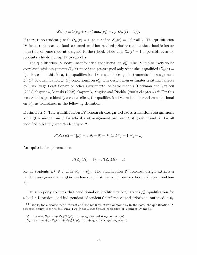
Definition 5. The qualification IV research design extracts a random assignment

for a gDA mechanism ϕ for school s at assignment problem X if given ϕ and X, for all

modified priority ρ and student type θ,

P (Zis(R) = 1|ρϕis = ρ, θi = θ) = P (Zis(R) = 1|ρϕis = ρ).

An equivalent requirement is

P (Zjs(R) = 1) = P (Zks(R) = 1)

for all students j, k ∈ I with ρϕjs = ρϕks. The qualification IV research design extracts a

random assignment for a gDA mechanism ϕ if it does so for every school s at every problem

X.

This property requires that conditional on modified priority status ρϕis, qualification for

school s is random and independent of students’ preferences and priorities contained in θi.

23That is, for outcome Yi of interest and the realized lottery outcome r0 in the data, the qualification IVresearch design uses the following Two Stage Least Square regression or a similar IV model:

Yi = α2 + β2Dis(r0) + Σkγk21{ρ

ϕis = k}+ ε2i (second stage regression)

Dis(r0) = α1 + β1Zis(r0) + Σkγk11{ρ

ϕis = k}+ ε1i (first stage regression)

24

Only under this conditionally random assignment does the qualification IV Zis generate

exogenous or random variation in assignment Dis.24 It turns out that no gDA mechanism

satisfies the above property even in the simple case with no priorities and unit capacities.

Proposition 2. Consider any sets of at least three students and at least three schools. Even

with no priorities (ρis = ρjs for all students i, j, and school s) and unit school capacities

(cs = 1 for all s), there exist student preference profiles at which every student ranks some

schools and the following holds: There is no gDA mechanism with any lottery regime for

which the qualification IV research design extracts a random assignment.

The proof is in Appendix A.3. I require every student to rank some school for excluding

uninteresting cases where students rank no school and have no effect on assignment outcomes.

I illustrate this result by an example.

Example 2. There are applicants 1, 2, 3, 4, 5 and schools A, B, C with the following

preferences and priorities:

�1 : B,A, ∅�2 : B, ∅�3 : C,A, ∅�4,�5 : C, ∅ρA, ρB, ρC : {1, 2, 3, 4, 5}.

The capacity of each school is 1. The treatment school is A.

Students 1 and 3 share the same modified priority ρϕiA for any gDA mechanism ϕ:

Both students 1 and 3 rank A second and have the same priority at A so that ρϕ1A ≡fϕ(ρ1A) + gϕ(rank1A) = fϕ(ρ3A) + gϕ(rank3A) ≡ ρϕ3A, which I denote by ρ. Nevertheless,

enumerating all possible lottery orders shows that for any gDA mechanism, we have

P (ZiA(R) = 1|ρϕiA = ρ, θi = θ1) = 2/3 6= 5/6 = P (ZiA(R) = 1|ρϕiA = ρ, θi = θ3) for STB

P (ZiA(R) = 1|ρϕiA = ρ, θi = θ1) = 2/3 6= 3/4 = P (ZiA(R) = 1|ρϕiA = ρ, θi = θ3) for MTB.

24Definition 5 for the qualification IV design may appear to be incomparable with Definition 2 for thefirst-choice design. However, Appendix B.1 shows that these two definitions are special cases of a unifieddefinition of a random assignment under general empirical research designs, including the first-choice andqualification IV designs. Hence, it is legitimate to use Definitions 2 and 5 to compare the two researchdesigns.

25

A computer program to implement this computation is available upon request. Therefore,

even with no priorities and unit capacities, the qualification IV research design does not

extract a random assignment for any gDA mechanism.25

Intuitively, the qualification IV research design fails in this example because students 1

and 3 experience different levels of competition at their first-choice schools B and C, respec-

tively, before applying for A. Let me consider the following cases.

Case i : Neither student 1 nor 3 applies for A, i.e., 1 and 3 are assigned B and C, respectively.

In this case, no student applies for A, and A is undersubscribed. Both 1 and 3 are therefore

qualified for A.

Case ii : Only student 1 applies for A. In this case, 1 is always assigned A and qualified

for A. By ρϕ1A = ρϕ3A shown above, student 3 is qualified for A if and only if 3 has a better

lottery number than 1 at A.

Case iii : Only student 3 applies for A. In this case, 3 is always assigned A and qualified for

A. Student 1 is qualified for A if and only if 1 has a better lottery number than 3 at A.

Case iv : Both students 1 and 3 apply for A. In this case, only one of 1 and 3 with a better

lottery number is assigned A and qualified for A.

For simplicity, consider the MTB lottery regime. Cases i and iv are ignorable since they

do not cause any difference between 1’s and 3’s qualification probabilities at A. Conditional

on Case ii, student 1 is qualified for sure while 3 is qualified with probability 0.5, the

probability that 3 has a better lottery number than 1 for A. Likewise, conditional on Case

iii, student 3 is qualified for sure, but 1 is qualified only with probability 0.5. Crucially,

Case iii is more likely to happen than Case ii. This is because 3’s first choice (C) is more

competitive than 1’s first choice (B) and so 3 is more easily rejected by the first choice

and more likely to apply for the second-choice school, A. As a result, 3 is more likely to

be qualified for A than 1 due to differential competition at their first-choice schools, as

the proof in Appendix A.3 makes it precise. The proof also generalizes this observation

25Since both ρϕ1A = ρϕ3A and ρ1A = ρ3A hold, the counterexample works even if I use original prioritiesto define an alternative qualification IV as Z ′

is(r) ≡ 1{ρis + ris ≤ max{ρjs + rjs|Djs(r) = 1}}. Also, notethat students 1 and 3 share the same priority at all schools in the above example. Thus, the qualification IVresearch design may fail even if I modify it to the more refined version that conditions on having the samepriority at all schools. Finally, the qualification IV research design does not extract a random assignmenteven for the top trading cycles mechanism, as shown in Section 5.3.

26

to any lottery regime and any market size. Section 5.2 shows that the problem with the

qualification IV holds up even if I modify its definition, e.g., by changing the priority cutoff

max{ρϕjs + rjs|Djs(r) = 1} to a constant number.

Example 2 illustrates a general point that students may have different qualification prob-

abilities depending on which schools they rank higher than the treatment school. This does

not matter for the first-choice design since students in the first-choice subsample Firsts(r0)

rank no school above the treatment school. Therefore, the above trouble does not happen

to the first-choice research design focusing on the first-choice subsample Firsts(r0). In this

sense, there are more threats to the qualification IV design than to the first-choice design.

Propositions 1 and 2 shed light on a contrast between the qualification IV and the first-

choice research designs. Unlike the first-choice research design, strategy-proofness for schools

is no longer sufficient for the qualification IV research design to extract a random assignment.

It may extract an unintended broken random assignment not only for the DA or top trading

cycles mechanism but also for the Boston mechanism and random serial dictatorship.

5 Discussion

5.1 Alternative Definition of a Random Assignment

My analysis of the first-choice design is based on Definition 2 of “random assignment.” This

definition requires that all students in realized fixed set Firsts(r0) share the same assignment

probability (propensity score). A possible alternative definition treats Firsts(R) as random

and requires that

P (Dis(R) = 1|i ∈ Firsts(R), θi = θ) = P (Dis(R) = 1|i ∈ Firsts(R))

for all i for whom these conditional probabilities are defined. R denotes the random (not

realized) lottery number profile. An equivalent property is

P (Djs(R) = 1|j ∈ Firsts(R)) = P (Dks(R) = 1|k ∈ Firsts(R))

for all j and k for whom these conditional probabilities are defined. This alternative def-

inition requires that treatment school assignment Dis(R) is independent of type θi or the

propensity score as a confounder conditional on random event i ∈ Firsts(R). This indepen-

dence conditional on a random event or statistic is reminiscent of Chamberlain (1980) and

Rosenbaum (1984)’s conditional logit panel frameworks, where the treatment distribution is

27

independent of individual heterogeneity conditional on the random empirical frequency of

being treated in the past.

All of my arguments extend to this alternative definition. See Appendix A.1 (especially

Remark 1) for why Theorem 1 is correct even under the alternative definition. The discus-

sion about the Boston mechanism under Example 1 in Section 3.3 goes through even under

the alternative definition since P (DiA(R) = 1|i ∈ FirstA(R), θi = θ) = 1/2 for i = 1, 2 and

is independent of θ. The analysis of the DA and Charlotte mechanisms in Example 1 in

Sections 3.1 and 3.4 also remains the same since in the example,

P (DiA(R) = 1|i ∈ FirstA(R), θi = θ1) = 1 6= 0 = P (DiA(R) = 1|i ∈ FirstA(R), θi = θ2),

where θ1 and θ2 denote student types having �1 and �2, respectively. This shows that the

first-choice design does not extract a random assignment even according to the alternative

definition.

5.2 Alternative Definitions of Research Designs

Constant Cutoff Qualification IV

Section 4 shows a potential problem with the qualification IV defined as Zis(r) ≡ 1{ρϕis+ris ≤max{ρϕjs + rjs|Djs(r) = 1}}, where max{ρϕjs + rjs|Djs(r) = 1} is a random priority cutoff

that varies as the lottery outcome changes. This problem may be expected to be solved by

a modification of the qualification IV. For any constant π ∈ R, define the constant cutoff

qualification IV by

Zπis(r) ≡ 1{ρϕis + ris ≤ π}.

In practice, the econometrician would define constant π as the realized priority cutoff at

school s, that is, π ≡ max{ρϕjs + r0js|Djs(r0) = 1} where r0 is the realized lottery numbers

in the data. The constant cutoff qualification IV trivially extracts a random assignment since

P (Zπis(R) = 1|ρϕis = ρ, θi = θ)

= P (ρϕis + ris ≤ π|ρϕis = ρ, θi = θ)

= P (ris ≤ π − ρϕis|ρϕis = ρ, θi = θ)

= π − ρ,

which is independent of θ conditional on ρϕis = ρ.

28

However, the constant cutoff qualification IV entails new problems apart from random-

ness. First, when using the realized priority cutoff π ≡ max{ρϕjs + r0js|Djs(r0) = 1}, I defineor select an instrument depending on the realized data. Such data-dependent model selec-

tion often makes standard statistical inference invalid (Leamer, 1978). In addition, perhaps

more importantly, the constant cutoff qualification IV may violate other requirements for a

valid IV than independence. It is about the “monotonicity” requirement for an IV. Let me

consider this issue with the following example.

Example 3. There are applicants 1, 2, 3, 4 and schools A and B with the following prefer-

ences and priorities:

�1,�2 : A,B, ∅�3,�4 : B, ∅ρA, ρB : {1, 2, 3, 4}.

The capacity of each school is 1. The treatment school is A. Without loss of generality, let

ρϕ1A = ρϕ2A = 0.

Consider two lottery outcomes at school A:

• rA ≡ (r1A, r2A, r3A, r4A) with r1A < r2A < r3A, r4A and r2A ≤ 0.5

• r′A ≡ (r′1A, r′2A, r

′3A, r

′4A) with r′3A, r

′4A < r′2A < r′1A and r′2A > 0.5.

Fix any lottery numbers rB at school B. Since r1A < r2A ≤ 0.5 and 0.5 < r′2A < r′1A,

by definition Z0.51A (rA, rB) = Z0.5

2A (rA, rB) = 1 and Z0.51A (r

′A, rB) = Z0.5

2A (r′A, rB) = 0. On the

other hand, for any gDA mechanism, D1A(rA, rB) = 1, D1A(r′A, rB) = 0, D2A(rA, rB) = 0,

and D2A(r′A, rB) = 1. This violates the monotonicity requirement for Z0.5

iA as an instrument

for DiA: Endogenous treatment variables D1A and D2A move in the opposite directions in

response to the same change in the IV from Z0.5iA = 1 to Z0.5

iA = 0. Monotonicity is required by

many modern IV models with heterogeneous behavior and treatment effects (Heckman and

Vytlacil (2007) chapter 4, Manski (2008) chapter 3, Angrist and Pischke (2009) section 4.4).

Therefore, while the constant cutoff qualification IV always extracts a random assignment,

it may not be able to identify a causal effect due to monotonicity violations.

Furthermore, since FirstA(r) = {1, 2} for all r in Example 3, this monotonicity violation

persists even if I restrict the sample to FirstA(r0). Also, since both ρϕ1A = ρϕ2A and ρ1A = ρ2A,

the counterexample goes through even if I use original priorities to define an alternative

constant cutoff qualification IV as Z0.5is (r) ≡ 1{ρiA + ris ≤ 0.5}. Finally, note that 1 and

29

2 share the same priority at all schools. Thus the constant cutoff qualification IV research

design may fail to satisfy monotonicity even if I modify it to the more restricted version that

conditions on having the same priority at all schools.

Constant Rank Qualification IV

Example 3 also shows that yet another potential modification of the qualification IV does

not extract a random assignment. For any positive integer m, define the constant rank

qualification IV by

Zm-this (r) ≡ 1{ris ≤ m-th({rjs|j ∈ I})},

where m-th(·) is the m-th order statistic.26 The constant rank qualification IV extracts a

random assignment since P (Zm-this (R) = 1|ρϕis = ρ, θi = θ) = m/|I|, which is independent of

θ. However,

• Z2nd1A (rA, rB) = Z2nd

2A (rA, rB) = 1(= Z0.51A (rA, rB) = Z0.5

2A (rA, rB)) and

• Z2nd1A (r′A, rB) = Z2nd

2A (r′A, rB) = 0(= Z0.51A (r

′A, rB) = Z0.5

2A (r′A, rB)).

Therefore, potential IV Z2ndiA violates monotonicity by the same reason for Z0.5

iA .27 The above

discussion also shows that the simplest possible IV, the random number ri itself, suffers from

the same monotonicity violation.

Conditioning on the Priorities at All Schools

Going back to the original first-choice and qualification IV research designs, they might fail

to extract a random assignment even if I modify them to the more refined version that

conditions on sharing the same priority at every school. Consider the following modification

of Example 1.

Example 4. There are applicants 1, 2, 3, and schools A and B with the following prefer-

ences and priorities:

�1 : A,B, ∅�2 : A, ∅

26Other possible definitions include Zm-this (r) ≡ 1{ρϕis + ris ≤ m-th({ρϕjs + rjs|j ∈ I, ρϕjs = ρϕis})} and

1{ρis+ris ≤ m-th({ρjs+rjs|j ∈ I, ρjs = ρis})}. The discussion below applies to these alternative definitionstoo.

27All of the above points in this section apply to the top trading cycles mechanism, as shown in the nextSection 5.3.

30

�3 : B,A, ∅ρA : 3, {1, 2}ρB : {1, 2, 3},

where student 3’s priority at school A is walk zone priority. The indifferences in the school

priorities are broken by STB. The capacity of each school is 1. The treatment school is A.

The only difference from Example 1 is ρB: School B is now indifferent among all students.

In Example 4, students 1 and 2 rank A first and share the same priority at both A and B.

However, students 1 and 2 do not share the same assignment probability at A for the DA or

Charlotte mechanism. Under the DA mechanism,

FirstA(r) =

∅ if r2 < r1 < r3

{1, 2} otherwise,

where ri is student i’s lottery number used by both schools. Nevertheless, enumerating all

lottery outcomes shows that for the treatment school assignment Dis and the qualifiation IV

Zis,

P (DiA(R) = 1|θi = θ1) = P (ZiA(R) = 1|θi = θ1) = 1/2

6= 1/3 = P (DiA(R) = 1|θi = θ2) = P (ZiA(R) = 1|θi = θ2).

Thus neither the first-choice or qualification IV research design extracts a random assignment

for the DA mechanism even if they condition on sharing the same priority at every school.

For the first-choice research design, this point remains true even if using the alternative

random assignment criterion in Section 5.1 since P (DiA(R) = 1|i ∈ FirstA(R), θi = θ1) =

3/5 6= 2/5 = P (DiA(R) = 1|i ∈ FirstA(R), θi = θ2).

Conditioning on the Whole Preference List

Likewise, conditioning on the whole preference list is not a solution. Consider yet another

modification of Example 1.

Example 5. There are applicants 1, 2, 3, and schools A and B with the following prefer-

ences and priorities:

�1 : A,B, ∅�2 : A,B, ∅

31

�3 : B,A, ∅ρA : 3, {1, 2}ρB : 1, 3, 2,

where student 3’s priority at school A and 1’s priority at B are walk zone priority. The

capacity of each school is 1. The treatment school is A.

In this example, students 2 shares the same preference list with 1, i.e., �1=�2. Nev-

ertheless, the first-choice and qualification IV research designs do not extract a random

assignment for the DA or Charlotte mechanism. Student 1 is assigned to A when 1 has a

better lottery number than 2 at A. Otherwise, 3 is assigned to A. Each of the two cases

occurs with equal probability 1/2. Thus,

P (D1A(R) = 1) = P (Z1A(R) = 1) = 1/2 6= 0 = P (Z2A(R) = 1) = P (D2A(R) = 1),

despite having

FirstA(r) =

{1, 2} if r1A < r2A

∅ otherwise.

Therefore, the first-choice or qualification IV research design does not necessarily extract a

random assignment for the DA or Charlotte mechanism even if one additionally conditions

on the entire preference list and requires every student to rank all schools. This means that

the potential problem with the first-choice design is not driven by short preferences.

5.3 Top Trading Cycles Mechanism

Some cities such as New Orleans and San Francisco have used a mechanism outside the gen-

eralized DA class studied in this paper. This mechanism, the top trading cycles mechanism,

is also advocated by researchers as a Pareto efficient mechanism that is strategy-proof for

students (Abdulkadiroglu and Sonmez, 2003). This mechanism is defined as follows.

Definition 6. The top trading cycles (TTC) mechanism creates a matching through

the following procedure. Take any assignment problem as given.

(1) Draw lottery number r according to a lottery regime (STB or MTB).

(2) Define school s’s ex post strict priority order �rs over students by i �rs i′ if ρis+ ris <

ρi′s + ri′s.

32

(3) Given �I and (�rs)s∈S, run the following top trading cycles algorithm (Shapley

and Scarf, 1974).

• Step t ≥ 1: Each student i points to her most preferred acceptable remaining

school (if any). Students who do not point to any school are assigned to ∅. Eachschool s points to its most preferred student. As there are a finite number of

schools and students, there exists at least one cycle, i.e., a sequence of distinct

schools and students (i1, s1, i2, s2, . . . , iL, sL) such that student i1 points to school

s1, school s1 points to student i2, student i2 points to school s2, . . . , student iL

points to school sL, and, finally, school sL points to student i1. Every student

il (l = 1, . . . , L) in any cycle is assigned to the school she is pointing to. Any

student who has been assigned a school seat or the outside option as well as any

school s which has been assigned students such that the number of them is equal

to its capacity cs is removed. If no student remains, the algorithm terminates.

Otherwise, it proceeds to the next step.

This algorithm terminates in a finite number of steps because at least one student is

matched with a school (or the outside option) at each step and there are only a finite

number of students.

It is possible to apply the first-choice research design to data from the TTC mechanism.

However, the TTC implementation of the first-choice research design turns out not to extract

a random assignment, as stated in Proposition 1. In Example 1, the TTC mechanism always

assigns 1 to A under all lottery realizations r (regardless of whether the lottery structure

is STB or MTB); no randomization occurs. Therefore, FirstA(r) = {1, 2} for all r, but

P (Dis(R) = 1|θi = θ1) = 1 6= 0 = P (Dis(R) = 1|θi = θ2). Thus the first-choice research

design does not extract a random assignment for the TTC mechanism.28

This failure of the first-choice research design is related to the fact that the TTC mech-

anism is not strategy-proof for schools. In Example 1, imagine A’s true preference is

3 �A 2 �A 1 while B’s is 1 �B 2 �B 3. Under these true preferences, A is matched

with 1. If A misreports 2 �′A 1, 3, however, A is matched with 2, who is preferred to 1 under

�A. Therefore, the TTC mechanism is not strategy-proof for A in Example 1. This provides

further support for the practical necessity of strategy-proofness for schools for successful

randomization under the first-choice research design.

The same example also implies that the qualification IV research design may fail for the

TTC mechanism. In fact, the qualification IV research design for the TTC mechanism does

28This point remains the same under the alternative definition of extracting a random assignment inSection 5.1: P (DiA(R) = 1|i ∈ FirstA(R), θi = θ1) = 1 6= 0 = P (DiA(R) = 1|i ∈ FirstA(R), θi = θ2).

33

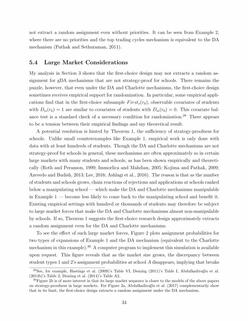
not extract a random assignment even without priorities. It can be seen from Example 2,

where there are no priorities and the top trading cycles mechanism is equivalent to the DA

mechanism (Pathak and Sethuraman, 2011).

5.4 Large Market Considerations

My analysis in Section 3 shows that the first-choice design may not extracts a random as-

signment for gDA mechanisms that are not strategy-proof for schools. There remains the

puzzle, however, that even under the DA and Charlotte mechanisms, the first-choice design

sometimes receives empirical support for randomization. In particular, some empirical appli-

cations find that in the first-choice subsample Firsts(r0), observable covariates of students

with Dis(r0) = 1 are similar to covariates of students with Dis(r0) = 0. This covariate bal-

ance test is a standard check of a necessary condition for randomization.29 There appears

to be a tension between their empirical findings and my theoretical result.

A potential resolution is hinted by Theorem 1, the sufficiency of strategy-proofness for

schools. Unlike small counterexamples like Example 1, empirical work is only done with

data with at least hundreds of students. Though the DA and Charlotte mechanisms are not

strategy-proof for schools in general, these mechanisms are often approximately so in certain

large markets with many students and schools, as has been shown empirically and theoreti-

cally (Roth and Peranson, 1999; Immorlica and Mahdian, 2005; Kojima and Pathak, 2009;

Azevedo and Budish, 2013; Lee, 2016; Ashlagi et al., 2016). The reason is that as the number

of students and schools grows, chain reactions of rejections and applications at schools ranked

below a manipulating school — which make the DA and Charlotte mechanisms manipulable

in Example 1 — become less likely to come back to the manipulating school and benefit it.

Existing empirical settings with hundred or thousands of students may therefore be subject

to large market forces that make the DA and Charlotte mechanisms almost non-manipulable

by schools. If so, Theorem 1 suggests the first-choice research design approximately extracts

a random assignment even for the DA and Charlotte mechanisms.

To see the effect of such large market forces, Figure 2 plots assignment probabilities for

two types of expansions of Example 1 and the DA mechanism (equivalent to the Charlotte

mechanism in this example).30 A computer program to implement this simulation is available

upon request. This figure reveals that as the market size grows, the discrepancy between

student types 1 and 2’s assignment probabilities at school A disappears, implying that breaks

29See, for example, Hastings et al. (2009)’s Table VI, Deming (2011)’s Table I, Abdulkadiroglu et al.(2014b)’s Table 2, Deming et al. (2014)’s Table A2.

30Figure 2b is of more interest in that its large market sequence is closer to the models of the above paperson strategy-proofness in large markets. For Figure 2a, Abdulkadiroglu et al. (2017) complementarily showthat in its limit, the first-choice design extracts a random assignment under the DA mechanism.

34

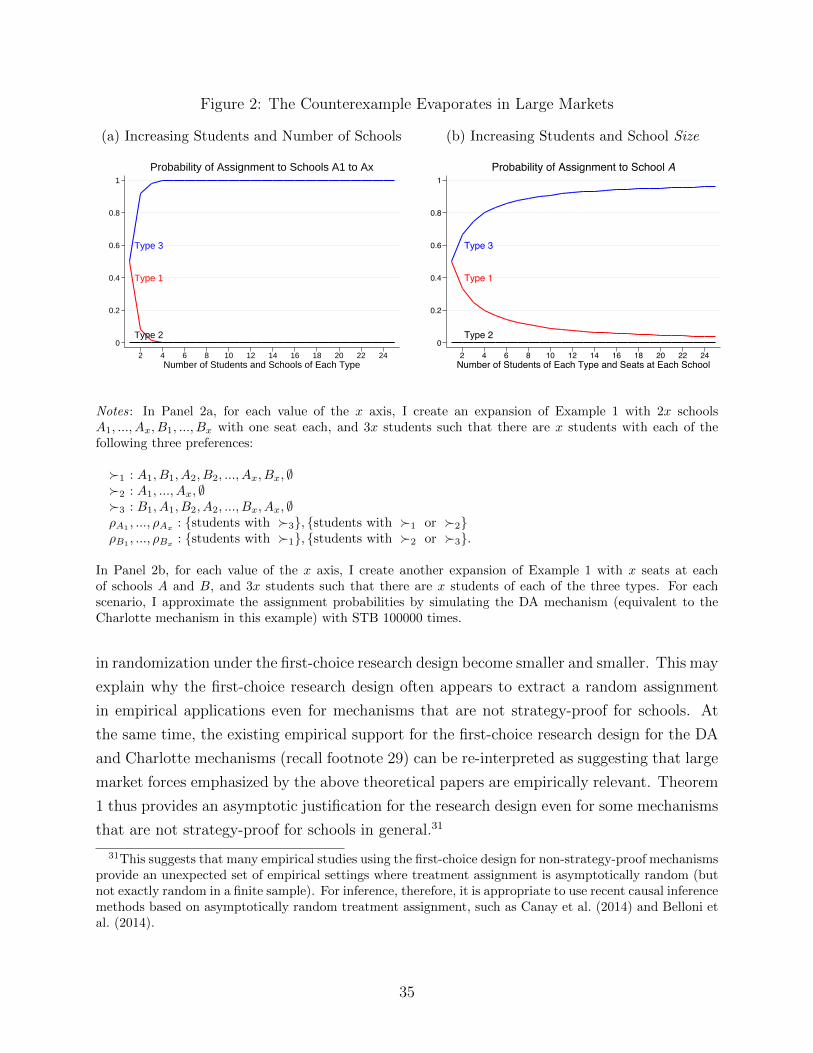
Figure 2: The Counterexample Evaporates in Large Markets

(a) Increasing Students and Number of Schools

Type 1

Type 2

Type 3

0

0.2

0.4

0.6

0.8

1

2 4 6 8 10 12 14 16 18 20 22 24Number of Students and Schools of Each Type

Probability of Assignment to Schools A1 to Ax

(b) Increasing Students and School Size

Type 1

Type 2

Type 3

0

0.2

0.4

0.6

0.8

1

2 4 6 8 10 12 14 16 18 20 22 24Number of Students of Each Type and Seats at Each School

Probability of Assignment to School A

Notes: In Panel 2a, for each value of the x axis, I create an expansion of Example 1 with 2x schoolsA1, ..., Ax, B1, ..., Bx with one seat each, and 3x students such that there are x students with each of thefollowing three preferences:

�1 : A1, B1, A2, B2, ..., Ax, Bx, ∅�2 : A1, ..., Ax, ∅�3 : B1, A1, B2, A2, ..., Bx, Ax, ∅ρA1

, ..., ρAx: {students with �3}, {students with �1 or �2}

ρB1, ..., ρBx

: {students with �1}, {students with �2 or �3}.

In Panel 2b, for each value of the x axis, I create another expansion of Example 1 with x seats at eachof schools A and B, and 3x students such that there are x students of each of the three types. For eachscenario, I approximate the assignment probabilities by simulating the DA mechanism (equivalent to theCharlotte mechanism in this example) with STB 100000 times.

in randomization under the first-choice research design become smaller and smaller. This may

explain why the first-choice research design often appears to extract a random assignment

in empirical applications even for mechanisms that are not strategy-proof for schools. At

the same time, the existing empirical support for the first-choice research design for the DA

and Charlotte mechanisms (recall footnote 29) can be re-interpreted as suggesting that large

market forces emphasized by the above theoretical papers are empirically relevant. Theorem

1 thus provides an asymptotic justification for the research design even for some mechanisms

that are not strategy-proof for schools in general.31

31This suggests that many empirical studies using the first-choice design for non-strategy-proof mechanismsprovide an unexpected set of empirical settings where treatment assignment is asymptotically random (butnot exactly random in a finite sample). For inference, therefore, it is appropriate to use recent causal inferencemethods based on asymptotically random treatment assignment, such as Canay et al. (2014) and Belloni etal. (2014).

35

6 Conclusion

This paper provides a formal basis for understanding when and why the two popular empirical

research designs do or do not extract a random assignment from school choice with lotteries.

The first-choice design does so for mechanisms that are strategy-proof for schools. On the

other hand, the qualification IV design does not necessarily extract a random assignment

for any mechanism, thus suggesting a difference between the two research designs. Table 1

in the introduction provides a summary of the main results.

This paper takes a step toward deciphering theoretical structures hidden in empirical

research designs exploiting market design with lotteries. This opens the door to several open

questions. The most ambitious agenda is to design assignment mechanisms that enable as

informative causal inference as possible (subject to welfare and strategic considerations). For

example, it is intriguing to compare the Boston, DA, and top trading cycles mechanisms with

different lottery regimes by their capabilities for quasi-experimental information production.

The contrast between positive Corollary 1 and negative Proposition 1 is a step toward such

a comparison. The empirically most important direction is to see if possible randomization

failures (in Propositions 1 and 2) cause significant biases in treatment effect estimates in real

data. I leave these challenging directions for future research.32

32There are many other directions of more technical nature. For example, while my framework assumesthe use of random lottery numbers, some existing empirical studies use data with regression-discontinuity-style tie-breaking by admissions test scores. I would expect the point of the current paper to be valideven in regression discontinuity situations, but it is open how to extend this paper’s results to a regressiondiscontinuity setting. Also, my results point to the importance of strategy-proofness for schools within mymechanism class. It is thus important to characterize or axiomatize mechanisms that are strategy-prooffor schools in the class. It is also a technical open question to use Theorem 1 and existing results onstrategy-proofness in the large to formally justify the first-choice research design in large markets.

36

References

Abdulkadiroglu, Atila and Tayfun Sonmez, “School Choice: A Mechanism Design

Approach,” American Economic Review, 2003, 93, 729–747.

, Josh Angrist, and Parag Pathak, “The Elite Illusion: Achievement Effects at Boston

and New York Exam Schools,” Econometrica, 2014, 82(1), 137–196.

, , Yusuke Narita, and Parag A. Pathak, “Research Design Meets Market Design:

Using Centralized Assignment for Impact Evaluation,” Econometrica, 2017.

, Weiwei Hu, and Parag Pathak, “Small High Schools and Student Achievement:

Lottery-Based Evidence from New York City,” 2014. Working Paper.

Agarwal, Nikhil and Paulo Somaini, “Demand Analysis using Strategic Reports: An

Application to a School Choice Mechanism,” 2015. Working Paper.

Ajayi, Kehinde, “Does School Quality Improve Student Performance? New Evidence from

Ghana,” 2013. Working Paper.

Angrist, Joshua D. and Jorn-Steffen Pischke, Mostly Harmless Econometrics: An

Empiricist’s Companion, Princeton University Press, 2009.

Angrist, Joshua, Peter Hull, Parag Pathak, and Christopher Walters, “Lever-

aging Lotteries for School Value-Added: Testing and Estimation,” Quarterly Journal of

Economics, 2016. Forthcoming.

Ashlagi, Itai, Yash Kanoria, and Jacob Leshno, “Unbalanced Random Matching Mar-

kets: The Stark Effect of Competition,” Journal of Political Economy, 2016, 125 (1),

69–98.

Azevedo, Eduardo and Eric Budish, “Strategyproofness in the Large,” 2013. Working

Paper.

Balinski, Michel and Tayfun Sonmez, “A Tale of Two Mechanisms: Student Place-

ment,” Journal of Economic Theory, 1999, 84, 73–94.

Belloni, Alexandre, Victor Chernozhukov, and Christian Hansen, “High-

Dimensional Methods and Inference on Structural and Treatment Effects,” Journal of

Economic Perspective, 2014, 28(2), 29–50.

37

Bergman, Peter, “The Effects of School Integration: Evidence from a Randomized Deseg-

regation Program,” 2016. Working Paper.

Beuermann, Diether, C Kirabo Jackson, and Ricardo Sierra, “Privately Managed

Public Secondary Schools and Academic Achievement in Trinidad and Tobago: Evidence

from Rule-Based Student Assignments,” 2016. Working Paper.

Bloom, Howard S and Rebecca Unterman, “Can Small High Schools of Choice Im-

prove Educational Prospects for Disadvantaged Students?,” Journal of Policy Analysis

and Management, 2014, 33 (2), 290–319.

Canay, Ivan A., Joseph P. Romano, and Azeem M. Shaikh, “Randomization Tests

under an Approximate Symmetry Assumption,” 2014. Working Paper.

Casella, George and Roger L Berger, Statistical Inference, Duxbury Pacific Grove, 2002.

Chamberlain, Gary, “Analysis of Covariance with Qualitative Data,” The Review of Eco-

nomic Studies, 1980, 47(1), 225–238.

Deming, David, “Better Schools, Less Crime?,” Quarterly Journal of Economics, 2011,

126(4), 2063–2115.

, Justine Hastings, Thomas Kane, and Douglas Staiger, “School Choice, School

Quality and Postsecondary Attainment,” American Economic Review, 2014, 104(3),

991–1013.

Dobbie, Will and Roland G. Fryer, “Exam High Schools and Academic Achievement:

Evidence from New York City,” American Economic Journal: Applied Economics, 2014,

6(3), 58–75.

Ergin, Haluk and Tayfun Sonmez, “Games of School Choice under the Boston Mecha-

nism,” Journal of Public Economics, 2006, 90, 215–237.

Fort, Margherita, Andrea Ichino, and Giulio Zanella, “Cognitive and Non-cognitive

Costs of Daycare 0-2 for Girls,” 2016. Working Paper.

Gale, David and Lloyd S. Shapley, “College Admissions and the Stability of Marriage,”

American Mathematical Monthly, 1962, 69, 9–15.

Hastings, Justine, Christopher Neilson, and Seth Zimmerman, “The Effect of

School Choice on Intrinsic Motivation and Academic Outcomes,” 2012. Working Paper.

38

, , and , “Are Some Degrees Worth More than Others? Evidence from College

Admission Cutoffs in Chile,” 2013. Working Paper.

, Thomas J. Kane, and Douglas O. Staiger, “Heterogenous Preferences and the

Efficacy of Public School Choice,” 2009. Working Paper.

Hatfield, John W., Fuhito Kojima, and Yusuke Narita, “Improving Schools Through

School Choice: A Market Design Approach,” Journal of Economic Theory, 2016. (Forth-

coming).

Heckman, James and Edward J. Vytlacil, “Econometric Evaluation of Social Programs

Part II,” Handbook of Econometrics, 2007, 6(B), 4875–5143.

Immorlica, Nicole and Mohammad Mahdian, “Marriage, Honesty, and Stability,”

SODA, 2005, pp. 53–62.

Jackson, Kirabo, “Do Students Benefit from Attending Better Schools? Evidence from

Rule-based Student Assignments in Trinidad and Tobago,” Economic Journal, 2010,

120(549), 1399–1429.

, “Single-sex Schools, Student Achievement, and Course Selection: Evidence from Rule-

based Student Assignments in Trinidad and Tobago,” Journal of Public Economics, 2012,

96(1-2), 173–187.

Kirkeboen, Lars, Edwin Leuven, and Magne Mogstad, “Field of Study, Earnings,

and Self-Selection,” Quarterly Journal of Economics, 2016.

Kojima, Fuhito and Parag A. Pathak, “Incentives and Stability in Large Two-Sided

Matching Markets,” American Economic Review, 2009, 99, 608–627.

Leamer, Edward E., Specification Searches: Ad Hoc Inference with Nonexperimental Data,

Wiley, 1978.

Lee, SangMok, “Incentive Compatibility of Large Centralized Matching Markets,” Review

of Economic Studies, 2016. Forthcoming.

Lucas, Adrienne and Isaac Mbiti, “Effects of School Quality on Student Achievement:

Discontinuity Evidence from Kenya,” American Economic Journal: Applied Economics,

2014, 6(3), 234–263.

Manski, Charles, Identification for Prediction and Decision, Cambridge: Harvard Univer-

sity Press, 2008.

39

McVitie, D. G. and L.B. Wilson, “Stable Marriage Assignments for Unequal Sets,” BIT,

1970, 10, 295–309.

Narita, Yusuke, “Match or Mismatch: Learning and Inertia in School Choice,” 2015.

Working Paper.

Pathak, Parag A and Jay Sethuraman, “Lotteries in Student Assignment: An Equiva-

lence Result,” Theoretical Economics, 2011, 6 (1), 1–17.

Pathak, Parag A. and Tayfun Sonmez, “Leveling the Playing Field: Sincere and So-

phisticated Players in the Boston Mechanism,” American Economic Review, 2008, 98(4),

1636–1652.

Pop-Eleches, Cristian and Miguel Urquiola, “Going to a Better School: Effects and

Behavioral Responses,” American Economic Review, 2013, 103(4), 1289–1324.

Rosenbaum, Paul R., “Conditional Permutation Tests and the Propensity Score in Ob-

servational Studies,” Journal of the American Statistical Association, 1984, pp. 565–574.

and Donald B. Rubin, “The Central Role of the Propensity Score in Observational

Studies for Causal Effects,” Biometrica, 1983, pp. 41–55.

Roth, Alvin E. and Elliott Peranson, “The Redesign of the Matching Market for Amer-

ican Physicians: Some Engineering Aspects of Economic Design,” American Economic

Review, 1999, 89, 748–780.

and Marilda A. O. Sotomayor, Two-sided Matching: a Study in Game-theoretic

Modeling and Analysis, Cambridge University Press: Econometric Society monographs,

1992.

Roth, Alvin E and Marilda Sotomayor, “The College Admissions Problem Revisited,”

Econometrica, 1989.

Shapley, Lloyd and Herbert Scarf, “On Cores and Indivisibility,” Journal of Mathemat-

ical Economics, 1974, 1, 23–28.

40

Appendix

A Proofs

A.1 Proof of Theorem 1

Preliminaries

I start with lemmas to prove Theorem 1. I use ϕ(r) as a shorthand for ϕ(ρ, r), the assignment

produced by a gDA mechanism ϕ when the reported priorities and lottery numbers are (ρ, r).

As per usual, a permutation of rs is a bijection from {ris}i∈I to {ris}i∈I itself.

Lemma 3. Consider any assignment problem X, any lottery number profile r, and any

gDA mechanism ϕ that is strategy-proof for schools. Let δs(r) be any permutation of rs

that switches only i′ and i′′ such that ρϕi′s = ρϕi′′s and min{ρϕi′s + ri′s, ρϕi′′s + ri′′s} > ρϕis + ris

for all i with Dis(r) = 1. That is, δi′s(r) = ri′′s, δi′′s(r) = ri′s, and δjs(r) = rjs for all

j 6= i′, i′′. If there are no such i′ and i′′, let δs(r) be the same as rs. For any such δs(r), I

have ϕ(r) = ϕ(δs(r), r−s).

Proof of Lemma 3. For any assignment problem, a deterministic assignment (or a matching)

is a vector µ that assigns each school s a set of at most cs students µs ⊂ I, and assigns each

student i a seat at a school or the outside option µi ∈ S∪{∅}. A matching µ is individually

rational if µi �i ∅ for every i ∈ I. With the notation ρϕ ≡ (ρϕis)i∈I,s∈S, µ is (ρϕ, r)-blocked

by (s, i) ∈ S × I if s �i µi and either |µs| < cs or there exists i ∈ I such that i �ϕrs i, i.e.,

ρϕis + ris < ρϕis+ ris. A matching µ is (ρϕ, r)-stable if it is individually rational and not

(ρϕ, r)-blocked by (s, i). I use the following facts.

Fact 1. (Roth and Sotomayor (1992)’s Theorem 5.8) For any assignment problem X, any

lottery number profile r, any gDA mechanism ϕ, any (ρϕ, r)-stable matching µ, any school s,

any preference �ϕs responsive with respect to (cs, ρ

ϕ, r), it holds µs �ϕs ϕs(ρ, r), where ϕs(ρ, r)

is the set of students assigned to s in the outcome of ϕ under X and r.

Fact 2. (Roth and Sotomayor (1989)’s Theorem 4) For any assignment problem X, any

lottery number profile r, and any gDA mechanism ϕ, let µ and µ′ be (ρϕ, r)-stable matchings

with µs �ϕs µ′

s for some preference �ϕs responsive with respect to (cs, ρ

ϕs , rs). Then, for any

i ∈ µs and i′ ∈ µ′s \ µs, it holds i �ϕ

rs i′, i.e., ρϕis + ris < ρϕi′s + ri′s.

Fact 3. Under any assignment problem, any lottery number profile r, any gDA mechanism

ϕ, any δs(r) satisfying the conditions in the statement of Lemma 3, every (ρϕ, r)-stable

matching is also (ρϕ, (δs(r), r−s))-stable.

41

Proof of Fact 3. Let µ be a (ρϕ, r)-stable matching. i′, i′′ 6∈ µs by Facts 1 and 2 and

the assumption that i′, i′′ 6∈ ϕs(ρ, r). The only potential (ρϕ, (δs(r), r−s))-blocking pairs

against µ are (s, i′) and (s, i′′) since the only difference between r and (δs(r), r−s) is the

positions of i′ and i′′ in rs. Since (1) both µ and ϕ(ρ, r) are (ρϕ, r)-stable and (2) min{ρϕi′s +ri′s, ρ

ϕi′′s + ri′′s} > ρϕis + ris for all i with Dis(r) = 1, Facts 1 and 2 imply that for any i ∈ µs,

ρϕis + ris < min{ρϕi′s + ri′s, ρϕi′′s + ri′′s} = min{ρϕi′s + δi′s(r), ρ

ϕi′′s + δi′′s(r)}, where the last

equality comes from ρϕi′s = ρϕi′′s. Neither (s, i′) nor (s, i′′) thus (ρϕ, (δs(r), r−s))-blocks µ.

Fact 4. Under any assignment problem, any lottery number profile r, any gDA mechanism

ϕ that is strategy-proof for schools, any δs(r) satisfying the conditions in the statement of

Lemma 3, every (ρϕ, (δs(r), r−s))-stable matching is also (ρϕ, r)-stable.

Proof of Fact 4. Suppose to the contrary that µ is (ρϕ, (δs(r), r−s))-stable but not (ρϕ, r)-

stable. I show that it contradicts the assumption that ϕ is strategy-proof for schools.

Step 4.1. Either student i′ or i′′ (but not both) is in µs.

Proof of Step 4.1. Case i : Suppose that neither i′ nor i′′ (but not both) is in µs. By

the (ρϕ, (δs(r), r−s))-stability of µ, neither (s, i′) or (s, i′′) does (ρϕ, (δs(r), r−s))-block µ.

Either (s, i′) or (s, i′′) does (ρϕ, r)-blocks µ, since (1) µ is (ρϕ, (δs(r), r−s))-stable and so

individually rational and (2) the only difference between r and (δs(r), r−s) is the positions

of i′ and i′′ in rs. That is, there exists i ∈ µs such that min{ρϕi′s + ri′s, ρϕi′′s + ri′′s} <

ρϕis + ris < min{ρϕi′s + δi′s(r), ρϕi′′s + δi′′s(r)} = min{ρϕi′s + ri′s, ρ

ϕi′′s + ri′′s}, a contradiction.

Case ii : Suppose that both i′ and i′′ are in µs. Since µ is not (ρϕ, r)-stable but is

individually rational (by its (ρϕ, (δs(r), r−s))-stability), there exists i such that s �i µi

and ρϕis + ris < max{ρϕi′s + ri′s, ρϕi′′s + ri′′s} = max{ρϕi′s + δi′s(r), ρ

ϕi′′s + δi′′s(r)}, a

contradiction to the (ρϕ, (δs(r), r−s))-stability of µ.

Step 4.2. ϕs(r) 6= ϕs(δs(r), r−s).

Proof of Step 4.2. i′, i′′ 6∈ ϕs(r) (by assumption), either i′ or i′′ is in µs (by Step

3.1), and Fact 3 implies that (ρϕ, r)-stable ϕs(r) is (ρϕ, (δs(r), r−s))-stable. Thus,

Facts 1 and 2 implies that for any �ϕδs responsive with respect to (cs, ρ

ϕs , (δs(r), r−s)),

it holds that ϕs(r) �ϕδs µs, where I use the fact that µ is not (ρϕ, r)-stable and so

µ 6= ϕ(r). Fact 1 implies that for any �ϕδs responsive with respect to (cs, ρ

ϕs , (δs(r), r−s)),

it holds that µs �ϕδs ϕs(δs(r), r−s). The two preference relations ϕs(r) �ϕδ

s µs and

µs �ϕδs ϕs(δs(r), r−s) jointly imply that for any �ϕδ

s responsive with respect to

(cs, ρϕs , (δs(r), r−s)), ϕs(r) �ϕδ

s ϕs(δs(r), r−s), implying ϕs(r) 6= ϕs(δs(r), r−s).

42

Step 4.3. ϕs(r) �ϕs ϕs(δs(r), r−s) for some preference�δ

s responsive with respect to (cs, ρs, δs(r)),

a contradiction to the assumption that ϕ is strategy-proof for schools.

Proof of Step 4.3. Take any �s responsive with respect to (cs, ρs, rs). If ϕs(δs(r), r−s) �s

ϕs(r), then it is a contradiction to the assumption that ϕ is strategy-proof for schools.

This implies ϕs(r) �s ϕs(δs(r), r−s) since ϕs(r) 6= ϕs(δs(r), r−s) as shown in Step 3.2.

Note that �s is also responsive with respect to (cs, ρs, δs(r)) since (1) the only difference

between r and (δs(r), r−s) is the positions of i′ and i′′ in rs, and (2) i′, i′′ 6∈ ϕs(r) by

assumption. Therefore, ϕs(r) �ϕs ϕs(δs(r), r−s) for some �δ

s responsive with respect to

(cs, ρs, δs(r)).

Facts 3 and 4 imply that under any assignment problem, any lottery number profile

r, any gDA mechanism ϕ that is strategy-proof for schools, any δs(r) satisfying the con-

ditions in the statement of Lemma 3, the set of (ρϕ, r)-stable matchings coincides with

the set of (ρϕ, (δs(r), r−s))-stable matchings. Each student or school except s has the

same set of responsive preferences over these common stable matchings both under r and

(δs(r), r−s). School s also has the same preference over these stable matchings both under r

and (δs(r), r−s) since (1) the only difference between r and (δs(r), r−s) is the positions of i′

and i′′ in rs, and (2) min{ρϕi′s + ri′s, ρϕi′′s + ri′′s} > ρϕis + ris for all i with Dis(r) = 1 and thus

Di′s(r) = Di′′s(r) = 0, which in turn implies i′, i′′ 6∈ µs for any (ρϕ, r)- or (ρϕ, (δs(r), r−s))-

stable matching µ. Therefore, the school pessimal (ρϕ, r)-stable matching is the same as the

school pessimal (ρϕ, (δs(r), r−s))-stable matching, i.e., ϕ(r) = ϕ(δs(r), r−s), proving Lemma

3.

Lemma 4. Consider any assignment problem X, any lottery number profile r, and any gDA

mechanism ϕ. Let δs(r) be any permutation of rs that switches only two students i′ and i′′

such that ρϕi′s = ρϕi′′s and there exists i with Dis(r) = 1 such that max{ρϕi′s+ ri′s, ρϕi′′s+ ri′′s} ≤

ρϕis + ris. If there are no such i′ and i′′, let δs(r) be the same as rs. For any such δs(r), I

have ϕ(r) = ϕ(δs(r), r−s).

Proof of Lemma 4. Under r or (δs(r), r−s), let t0 be the step in the DA algorithm at which

either i′ or i′′ or both first apply for s. If there is no such a step t0 under either r or

(δs(r), r−s), then the DA algorithm works in the same way until its end both under r and

(δs(r), r−s), completing the proof. Assume the existence of such a step t0 under both r and

(δs(r), r−s). Until step t0 − 1, the DA algorithm operates in the same way both under r and

(δs(r), r−s) since the only difference between the two situations is the positions of i′ and i′′

in rs. t0 is thus common to r and (δs(r), r−s). Let Ist0 be the set of students who are kept

43

by s from step t0 − 1 or newly apply for s in step t0. Ist0 is again the same between r and

(δs(r), r−s). There are a few cases to consider.

Case I : Both i′ and i′′ apply for s at step t0. Under r, s tentatively accepts both i′ and i′′

by the assumption that there exists i with Dis(r) = 1 such that max{ρϕi′s+ ri′s, ρϕi′′s+ ri′′s} ≤

ρϕis + ris. Under (δs(r), r−s), s again tentatively accepts both i′ and i′′. This is because

{ρϕis + ris}i∈Ist0 = {ρϕis + δi(rs)}i∈Ist0 (recall i′, i′′ ∈ Ist0 by assumption and Ist0 is the same

between r and (δs(r), r−s)) and the above fact that s tentatively accepts both i′ and i′′ under

r, which jointly imply that max{ρϕi′s+δi′s(r), ρϕi′′s+δi′′s(r)} = max{ρϕi′s+ri′s, ρ

ϕi′′s+ri′′s} ≤ cs-

th({ρϕis + ris}i∈Ist0 ) where cs-th(·) is the cs-th order statistic. The DA algorithm also works

in the same way for the remaining steps.

Case II : Only one of i′ or i′′ applies for s at step t0. Without loss of generality, suppose

only i′ applies for s at step t0. Under r, s tentatively accepts i′ by the assumption that there

exists i with Dis(r) = 1 such that ρϕi′s + ri′s ≤ max{ρϕi′s + ri′s, ρϕi′′s + ri′′s} ≤ ρϕis + ris.

Case II.A: ri′s > ri′′s (and so δi′s(r) < δi′′s(r)). Under (δs(r), r−s), s also tentatively

accepts i′ by the following reason. By the above fact that s tentatively accepts i′ under r,

it holds that ρϕi′s + ri′s ≤ cs-th({ρϕis + ris}i∈Ist0 ), implying ρϕi′s + δi′s(r) < ρϕi′s + ri′s ≤ cs-

th({ρϕis + δis(r)}i∈Ist0 ).

Case II.B : ri′s < ri′′s. Under (δs(r), r−s), s also tentatively accepts i′ by the fol-

lowing reason. Suppose not. Then cs-th({ρϕis + ris}i∈Ist0 ) ≤ cs-th({ρϕis + δi(rs)}i∈Ist0 ) <

ρϕi′s + δi′s(r) = ρϕi′′s + ri′′s, where the first inequality ri′s < ri′′s and the last equality uses

the assumption ρϕi′s = ρϕi′′s. Let’s call cs-th({ρϕis + ris}i∈Ist0 ) the tentative cutoff for school

s at step t0, which is common between r and (δs(r), r−s) since Ist0 is the same between

r and (δs(r), r−s) and ris = δis(r) for all i ∈ Ist \ i′. Since the tentative cutoff is mono-

tonically decreasing in steps, the above inequality implies that for all i with Dis(r) = 1,

ρϕis + ris < ρϕi′s + δi′s(r) = ρϕi′′s + ri′′s, contradicting the assumption that there exists i with

Dis(r) = 1 such that ρϕi′′s + ri′′s ≤ max{ρϕi′s + ri′s, ρϕi′′s + ri′′s} ≤ ρϕis + ris.

In all cases, the DA algorithm works in the same way at step t0 under r and (δs(r), r−s).

In Case I, the DA algorithm also works in the same way for the remaining steps. In Case

II, let t1 be the step in the DA algorithm at which i′′ first applies for s. If there is no such

a step t1 under either r or (δs(r), r−s), then the DA algorithm works in the same way until

its end both under r and (δs(r), r−s), completing the proof. Assume the existence of such a

44

step t1 under both r and (δs(r), r−s). Until step t1 − 1, the DA algorithm operates in the

same way both under r and (δs(r), r−s) since the only difference between the two situations

is the positions of i′ and i′′ in rs. t1 is thus common to r and (δs(r), r−s). Let Ist1 be the set

of students who are kept by s from step t1 − 1 or newly apply for s in step t1. Ist1 is again

the same between r and (δs(r), r−s). I again consider the following two cases.

Case II.A (Continued): ri′s > ri′′s. Under (δs(r), r−s), s also tentatively accepts i′′ by

the following reason. Suppose not. Then cs-th({ρϕis+ ris}i∈Ist1 ) ≤ cs-th({ρϕis+ δi(rs)}i∈Ist1 ) <ρϕi′′s+ δi′′s(r) = ρϕi′s+ ri′s. Since the tentative cutoff is monotonically decreasing in steps, the

above inequality implies that for all i with Dis(r) = 1, ρϕis + ris < ρϕi′s + δi′s(r) = ρϕi′′s + ri′′s,

contradicting the assumption that there exists i with Dis(r) = 1 such that ρϕi′′s + ri′′s ≤max{ρϕi′s + ri′s, ρ

ϕi′′s + ri′′s} ≤ ρϕis + ris.

Case II.B (Continued): ri′s < ri′′s. By the above fact that s tentatively accepts i′′

under r, it holds that ρϕi′′s + ri′′s ≤ cs-th({ρϕis + ris}i∈Ist1 ), implying ρϕi′′s + δi′′s(r) < cs-

th({ρϕis + δis(r)}i∈Ist1 ).

In both cases, the DA algorithm works in the same way at step t1 under r and (δs(r), r−s).

Since both i0 and i1 have already applies for s by step t1 or never apply for s, the DA

algorithm also works in the same way for the remaining steps, showing Lemma 4.

Main Proof

Suppose that the first-choice research design does not extract a random assignment for gDA

mechanism ϕ for some school s at some assignment problem X. Fix ϕ, s, and X throughout.

I show that this supposition implies that ϕ is not strategy-proof for schools. For each lottery

number profile r, define i0(r) and i1(r) by two students who satisfy the following conditions.

• i0(r), i1(r) ∈ Firsts(r)

• Di0(r)s(r) = 0 and Di1(r)s(r) = 1

• ri0(r)s ≤ ris for all i ∈ Firsts(r) with Dis(r) = 0

• ri1(r)s ≥ ris for all i ∈ Firsts(r) with Dis(r) = 1.

If there are no two students satisfying the conditions, let i0(r) = i1(r) = ∅. i0(r) and i1(r)

are uniquely well-defined for all r. (If there are two i0(r) 6= i0(r) satisfying the conditions,

then ri0(r)s > ri0(r)s and ri0(r)s < ri0(r)s, a contradiction. The same logic holds for i1(r) too.)

This proof uses the following equivalent representation of gDA mechanism ϕ.

45

Definition 7. Algorithm 2STAGES(r) operates in the following way.

(1) Same as in Definition 1.

(2) Same as in Definition 1.

(3) Given �I and (�ϕrs)s∈S, run the following sub-algorithm STAGE1(r): Remove i0(r)

and i1(r) from X (without changing anything else) and run the DA algorithm on the

remaining subproblem where schools’ strict priorities are given by (�ϕrs).

(4) Starting from the output of STAGE1(r) as the initial tentative assignment, run the

following sub-algorithm STAGE2(r): Include i0(r) and i1(r) and run the DA algorithm

where only i0(r) and i1(r) apply for any school and schools’ strict priorities are given

by (�ϕrs).

By McVitie and Wilson (1970)’s order irrelevance result, 2STAGES(r) and ϕ(r) (the simplified

notation for ϕ(ρ, r)) produce the same matching for all r. Let t − 1 be the last step of

STAGE1(r) at which STAGE1(r) stops and µt−1(r) ≡ (µst−1(r))s∈S be the tentative matching

at the end of step t − 1. Start counting STAGE2(r)’s steps without resetting the step index

so that t is the initial step of STAGE2(r). (Note that t implicitly depends on r.)

For each lottery number profile r, define σ∗(r) = (σ∗s′(r))s′∈S as the following permutation

of r. If i0(r) = i1(r) = ∅, then σ∗is(r) = ris for all student i and school s. Otherwise, if gDA

mechanism ϕ uses MTB, σ∗(r) is obtained by switching only i0(r) and i1(r) only in rs, i.e.,

• σ∗i0(r)s

(r) = ri1(r)s and σ∗i1(r)s

(r) = ri0(r)s

• σ∗is(r) = ris for all i 6= i0(r), i1(r)

• σ∗is′(r) = ris′ for all i and s′ 6= s.

If ϕ uses STB, σ∗(r) is obtained by switching i0(r) and i1(r) in rs′ for all s′, i.e., for all

s′ ∈ S, including s,

• σ∗i0(r)s′

(r) = ri1(r)s′ and σ∗i1(r)s′

(r) = ri0(r)s′

• σ∗is′(r) = ris′ for all i 6= i0(r), i1(r).

Given any r, I say two students i′ and i′′ are consecutive in rs within Firsts(r) if

i′, i′′ ∈ Firsts(r) and there is no i′′′ ∈ Firsts(r) such that ri′s < ri′′′s < ri′′s or ri′s > ri′′′s >

ri′′s. For each r, consider any permutation σs(r) 6= σ∗s(r) of rs that switches only two students

i′ and i′′ who are consecutive in rs within Firsts(r), i.e., σi′s(r) = ri′′s, σi′′s(r) = ri′s, and

σjs(r) = rjs for all j 6= i′, i′′. If there are no such i′ and i′′, let σs(r) = rs. Let σ(r) be the

following. If ϕ uses MTB, let σ(r) = (σs(r), r−s). If ϕ uses STB, let σ(r) = ×|S|σs(r).

46

Lemma 5. (A breakdown of the Fisher property discussed in Section 3.3) There exits lot-

tery number profile r consistent with gDA mechanism ϕ’s lottery structure (STB or MTB)

satisfying the following: Di0(r)s(σ∗(r)) = Di1(r)s(σ

∗(r)) = 0 or there exist some student

i ∈ Firsts(r) and some permutation σs(r) defined above such that Dis(σ(r)) 6= Dis(r).

Proof of Lemma 5. It is enough to show that if there is no r such that there exists

i ∈ Firsts(r) such that Dis(σ(r)) 6= Dis(r), then there exits r such that Di0(r)s(σ∗(r)) =

Di1(r)s(σ∗(r)) = 0. Suppose to the contrary that for all r, it is not the case Di0(r)s(σ

∗(r)) =

Di1(r)s(σ∗(r)) = 0.

Step 5.A. For all lottery number profile r with i0(r) 6= ∅ and i1(r) 6= ∅, Di0(r)s(σ∗(r)) =

1, Di1(r)s(σ∗(r)) = 0, and Dis(σ

∗(r)) = Dis(r) for all student i ∈ Firsts(r) with i 6= i0(r) and

i 6= i1(r).

Proof of Step 5.A. By the above assumption that for all r, it is not the case

Di0(r)s(σ∗(r)) = Di1(r)s(σ

∗(r)) = 0, it is enough to show that for all such r,

Di1(r)s(σ∗(r)) = 0 and Dis(σ

∗(r)) = Dis(r) for all i ∈ Firsts(r) with i 6= i0(r) and

i 6= i1(r). Let me consider STAGE1(r) and STAGE1(σ∗(r)). Since everything except

i0(r) and i1(r)’s lottery numbers is the same between r and σ∗(r), both STAGE1(r) and

STAGE1(σ∗(r)) produce the same tentative assignment µst−1(r) = µst−1(σ∗(r)) ≡ µst−1.

Now start STAGE2(r) and STAGE2(σ∗(r)). Under r, McVitie and Wilson (1970)’s or-

der irrelevance result implies s rejects i0(r) and tentatively accepts i1(r), which implies

ρϕi0(r)s+ri0(r)s > cs-th({ρϕis+ris}i∈µst−1∪i0(r)∪i1(r)) where cs-th(·) is the cs-th order statistic

in the input set. Under σ∗(r), by definition of σ∗(r), ρϕi1(r)s+σ∗i1(r)s

(r) = ρϕi0(r)s+ ri0(r)s >

cs-th({ρϕis+ris}i∈µst−1∪i0(r)∪i1(r)), resulting in s’s rejecting i1(r). Since any rejected student

is never be accepted in the DA algorithm, this implies Di1(r)s(σ∗(r)) = 0. Dis(σ

∗(r)) =

Dis(r) for all i ∈ Firsts(r) with i 6= i0(r) and i 6= i1(r) by the following reason. Suppose

not. There exists i ∈ µst−1 ∩ Firsts(r) \ {i0(r), i1(r)} for whom, without loss of general-

ity, Dis(σ∗(r)) = 0 and Dis(r) = 1. This implies that Di0(r)s(σ

∗(r)) = Di1(r)s(σ∗(r)) = 0

since ρϕis + ris < ρϕi1(r)s + ri1(r)s < ρϕi0(r)s + ri0(r)s (the first inequality is by definition of

i1(r)) and so ρϕis + σ∗is(r) < ρϕi0(r)s + σ∗

i0(r)s(r) < ρϕi1(r)s + σ∗

i1(r)s(r). This is a contradiction

to the assumption that for all r, it is not the case Di0(r)s(σ∗(r)) = Di1(r)s(σ

∗(r)) = 0.

Step 5.B. For all lottery number profile r with i0(r) = i1(r) = ∅, it holds ϕ(σ∗(r)) = ϕ(r). For

each r and each permutation σ(r) 6= σ∗(r) defined right before Lemma 5, Dis(σ(r)) = Dis(r)

for all i ∈ Firsts(r).

47

Proof of Step 5.B. For all r with i0(r) = i1(r) = ∅, σ∗(r) = r and it is trivial that

ϕ(σ∗(r)) = ϕ(r). The second part is by assumption.

Step 5.C. For each lottery number profile r, define os(r) ≡ |{i ∈ Firsts(r)|Dis(r) = 1}|. Foreach r and each permutation σs(r) of rs that permutes lottery numbers only among members

of Firsts(r), let σ(r) be the following. If ϕ uses MTB, σ(r) = (σs(r), r−s). If ϕ uses STB,

σ(r) = ×|S|σs(r). Then the following is true for all r.

(1) Firsts(σ(r)) = Firsts(r).

(2) os(σ(r)) = os(r).

(3) For all i and i′ in Firsts(σ(r)), if Dis(σ(r)) > Di′s(σ(r)), then σis(r) < σi′s(r).

Proof of Step 5.C. Since any permutation can be expressed as a composition of

contrapositions (permutations switching consecutive two elements), I can express any σ

as a composition of σ∗ and σ’s defined right before Lemma 5. Steps 5.A and 5.B imply

(1) and (2). (3) follows from the fact that for all r and all i, i′ ∈ Firsts(r), ρϕis = ρϕi′s

and another well-known property of the DA algorithm that for applicants who rank s

first and share ρϕis, Dis is monotonically decreasing in ris (Balinski and Sonmez, 1999).

Let R ≡ {r ∈ [0, 1]|I|×|S||ris 6= rjs for all students i, j, and school s} be the set of all

possible values of the lottery number profile r. Partition R into P ≡ {Rn}n∈N (N is an

uncountable set of indices) such that the following holds: Within eachRn, for all r, r′ ∈ Rn, r

can be obtained from r′ by permutation r′ = σ(r), where σ(r) is a permutation of r defined

in Step 5.C. This partition is well-defined by Step 5.C(1): Since Step 5.C(1) guarantees

Firsts(r) = Firsts(r′), r′ = σ(r) for such a permutation σ if and only if r = σ(r′) for

such a (possibly different) permutation σ. Let rn be a generic element of Rn. Note that

Firsts(rn) and os(rn) are the same for all rn ∈ Rn by Step 5.C(1) and 5.C(2), respectively.

Step 5.C guarantees that conditional on each Rn, Dis(R) is independent of i’s type for all

i ∈ Firsts(rn), i.e., for all n and θ, assuming the rule of 0/0 = 0,

P (Dis(R) = 1|i ∈ Firsts(rn), R ∈ Rn, θi = θ) =os(rn)

|Firsts(rn)|1{Firsts(rn) 6= ∅},

which is independent of θi = θ. The equality holds since Firsts(rn) and os(rn) stay constant

across all rn ∈ Rn and under each rn, students with the os(rn)-best lottery numbers have

Dis(rn) = 1 (by Step 5.C). Therefore, for each n ∈ N ,

48

P (Dis(R) = 1|i ∈ Firsts(r0), R ∈ Rn, θi = θ)

=

os(rn)

|Firsts(rn)|if ρϕis = ρϕjs for any j ∈ Firsts(rn) 6= ∅

1 if ρϕis < ρϕjs for any j ∈ Firsts(rn) 6= ∅

or (Firsts(rn) = ∅ and Dks(rn) = 1 for all k ∈ Firsts(r0))

0 otherwise≡ pn,

where pn is independent of θi conditional on i ∈ Firsts(r0) since pn depends on θi only

through ρϕis, but ρϕis is pinned down by the fact that i ∈ Firsts(r0).

Let Y be Y (R) = RRn where RR

n is the element of the partition P with R ∈ RRn . Let PY

be the probability measure of Y induced by that of R, i.e. for all A ⊂ N , PY ({Rn}n∈A) ≡P (R ∈ ∪n∈ARn). With this notation, assuming the rule of 0/0 = 0,

P (Dis(R) = 1|i ∈ Firsts(r0), θi = θ)

=

∫{Rn}n∈N

P (Dis(R) = 1|i ∈ Firsts(r0), Y = Rn, θi = θ)dPY (Rn)

(by the law of iterated expectation)

=

∫{Rn}n∈N

pndPY (Rn),

which is again independent of θi since both pn and PY are independent of θi. Thus the

first-choice research design extracts a random assignment, a contradiction. This completes

the proof of Lemma 5.

Remark 1. Under the alternative definition of a random assignment in Section 5.1, the last

part of the proof of Lemma 5 simplifies to the following.

P (Dis(R) = 1|i ∈ Firsts(R), θi = θ)

=

∫{Rn}n∈N

P (Dis(R) = 1|i ∈ Firsts(R), Y = Rn, θi = θ)dPY (Rn)

=

∫{Rn}n∈N

os(rn)

|Firsts(rn)|1{Firsts(rn) 6= ∅}dPY (Rn),

which is independent of θi = θ. No other part of the proof depends on which random assign-

ment definition I use. Therefore, Theorem 1 goes through even for the random assignment

definition in Section 5.1.

Lemma 5 shows two possible scenarios. I consider these two cases, Cases 1 and 2 below, one

by one.

49

Case 1: There exists lottery number profile r consistent with gDA mechanism ϕ’s lottery

structure (STB or MTB) such that Di0(r)s(σ∗(r)) = Di1(r)s(σ

∗(r)) = 0. For each r, define r∗s

as the following permutation of rs. If i0(r) = i1(r) = ∅, let r∗is = ris for all student i and

school s. Otherwise, let r∗s be defined by the following conditions.

• r∗is = ris for all i with ρϕis 6= ρϕi0(r)s = ρϕi1(r)s

• r∗i1(r)s = max{ris|ρϕis = ρϕi0(r)s = ρϕi1(r)s and Dis(r) = 1}

• r∗i0(r)s > r∗i1(r)s and there is no such i that ρϕis = ρϕi0(r)s = ρϕi1(r)s and r∗i0(r)s > r∗is > r∗i1(r)s

• r∗is > r∗js if and only if ris > rjs for all i, j such that ρϕis = ρϕjs = ρϕi0(r)s = ρϕi1(r)s and

i 6= i0(r), i 6= i1(r), j 6= i0(r), and j 6= i1(r).

For each lottery number profile r and each school s′ 6= s, define σs′(r) as the following

permutation of rs′ . If i0(r) = i1(r) = ∅ or MTB is used by ϕ, then σis′(r) = ris′ for all

student i. Otherwise, σs′(r) is obtained by moving i1(r) to right above i0(r), i.e.,

• σi1(r)s′(r) = max{ris′|ris′ < ri0(r)s′}

• σis′(r) > σjs′(r) if and only if ris′ > rjs′ for all students i, j such that i, j 6= i1(r).

Note that σs′(r) implicitly depends on whole r.

Lemma 6. (Outcome-equivalence between lottery number profiles r and (r∗s , σ−s(r))) For all

lottery number profile r, I have ϕ(r) = ϕ(r∗s , σ−s(r)) where σ−s(r) ≡ (σs′(r))s′ 6=s. There-

fore, Di0(r)s(r∗s , σ−s(r)) = 0(= Di0(r)s(r)) and Di1(r)s(r

∗s , σ−s(r)) = 1(= Di1(r)s(r)) whenever

i0(r), i1(r) 6= ∅.

Proof of Lemma 6. The following Steps 6.A and 6.B imply Lemma 6.

Step 6.A. For all lottery number profile r, ϕ(r) = ϕ(r∗s , r−s).

50

Proof of Step 6.A. If i0(r) = i1(r) = ∅ and so r∗s = rs, the above equality is trivial.

Otherwise, r∗s is obtained from rs through a composition of two permutations. The first

one permutes lottery numbers only among students in some set I1 such that ρϕi′s = ρϕi′′s for

all i′, i′′ ∈ I1 and there exists i with Dis(r) = 1 such that maxi′∈I1{ρϕi′s + ri′s} ≤ ρϕis + ris.

The second permutation permutes lottery numbers only among students in some set I0

such that ρϕi′s = ρϕi′′s for all i′, i′′ ∈ I0 and mini′∈I0{ρϕi′s + ri′s} > ρϕis + ris for all i with

Dis(r) = 1. The first permutation is a composition of special permutations δ satisfying

the conditions in Lemma 4. If ϕ is not strategy-proof for schools, then the proof of

Theorem 1 is complete. If ϕ is strategy-proof for schools, the second permutation is a

composition of special permutations δ satisfying the conditions in Lemma 3. Therefore

Lemmas 3 and 4 imply Step 2.A.

Step 6.B. For all lottery number profile r, ϕ(r∗s , r−s) = ϕ(r∗s , σ−s(r)).

Proof of Step 6.B. If i0(r) = i1(r) = ∅ and so σ−s(r) = r−s, the above inequality is

trivial. Otherwise, at the first step of the DA algorithm constituting ϕ, students apply

for schools in the same way both under (r∗s , r−s) and (r∗s , σ−s(r)). In particular, i1(r)

applies for s since i1(r) ∈ Firsts(r). Schools also tentatively accept students in the

same way both under (r∗s , r−s) and (r∗s , σ−s(r)): s does so since s has the same strict

priority �ϕr∗s

both under (r∗s , r−s) and (r∗s , σ−s(r)). The other schools also do so since

the only possible difference between �ϕrs′

and �ϕσs′ (r)

is the position of i1(r), who applies

for s. As a result, since Step 2.A implies Di1(r)s(r∗s , r−s) = 1, s tentatively accepts i1(r)

at the first step of the DA algorithm both under (r∗s , r−s) and (r∗s , σ−s(r)). Since (a) s

has the same preference �ϕr∗s

both under (r∗s , r−s) and (r∗s , σ−s(r)), (b) the only possible

difference between �ϕrs′

and �ϕσs′ (r)

is the position of i1(r), and (c) i1(r) is tentatively

kept by s and is never be rejected by s under (r∗s , r−s), the DA algorithm operates in

the same way for the remaining steps, producing the same matching.

Lemma 7. (Partial outcome-equivalence between σ∗(r) and (σ∗s(r

∗s , r−s), σ−s(r))) For all lot-

tery number profile r with Di0(r)s (σ∗(r)) = Di1(r)s(σ

∗(r)) = 0, it is the case that Di0(r)s(σ∗s(r

∗s , r−s),

σ−s(r)) = Di1(r)s(σ∗s(r

∗s , r−s), σ−s(r)) = 0.

Proof of Lemma 7. If i0(r) = i1(r) = ∅ and so σ∗(r) = r = (σ∗s(r

∗s , r−s), σ−s(r)), Lemma 7 is

immediate. Otherwise, I first prove the following result.

Step 7.A. For all lottery number profile r with Di0(r)s(σ∗(r)) = Di1(r)s(σ

∗(r)) = 0, it is the

case ϕ(σ∗(r)) = ϕ(σ∗s(r

∗s , r−s), σ

∗−s(r)).

51

Proof of Step 7.A. Note that

a) σ∗i0(r)s

(r) = ri1(r)s ≤ min{ri0(r)s, r∗i0(r)s, r∗i1(r)s

} = min{σ∗i1(r)s

(r), σ∗i1(r)s

(r∗s , r−s), σ∗i0(r)s

(r∗s , r−s)}, where the last equality follows from i0(r∗s , r−s) = i0(r) and i1(r

∗s , r−s) = i1(r)

by Step 2.A.

b) ρϕjs + σ∗js(r) > ρϕis + σ∗

is(r) for all j with ρϕjs = ρϕi0(r)s and σ∗js(r) > σ∗

i0(r)s(r) and all i

with Dis(σ∗(r)) = 1 since Di0(r)s(σ

∗(r)) = 0 by assumption and i0(r) ∈ Firsts(r) and so

i0(r) ranks s first.

(a) and (b) imply that starting from σ∗(r), σ∗s(r

∗s , r−s) is obtained from σ∗

s(r) through

a permutation that permutes lottery numbers only among students in some set I0 such

that ρϕi′s = ρϕi′′s for all i′, i′′ ∈ I0 and mini′∈I0{ρϕi′s + σ∗

i′s(r)} > ρϕis + σ∗is(r) for all i with

Dis(σ∗(r)) = 1. This permutation is a composition of special permutations δ’s that

satisfy the conditions in Lemma 3. Therefore Lemmas 3 and 4 imply Step 7.A.

Now let me compare ϕ(σ∗s(r

∗s , r−s), σ

∗−s(r)) and ϕ(σ∗

s(r∗s , r−s), σ−s(r)). At the first step

of the DA algorithm constituting ϕ, students apply for schools in the same way both under

(σ∗s(r

∗s , r−s), σ

∗−s(r)) and (σ∗

s(r∗s , r−s), σ−s(r)). In particular, i0(r) and i1(r) apply for s since

i0(r), i1(r) ∈ Firsts(r). Schools also tentatively accept students in the same way both under

(σ∗s(r

∗s , r−s), σ

∗−s(r)) and (σ∗

s(r∗s , r−s), σ−s(r)): s does so since s has the same strict priority

�ϕσ∗s (r

∗s ,r−s)

both under (σ∗s(r

∗s , r−s), σ

∗−s(r)) and (σ∗

s(r∗s , r−s), σ−s(r)). The other schools also

do so since the only possible differences between �ϕσ∗s′ (r)

and �ϕσs′ (r)

are the positions of i0(r)

and i1(r), both of whom apply for s.

If s rejects both i0(r) and i1(r) at the first step, the proof is complete. Otherwise, s

tentatively accepts at least i0(r) since ρϕi0(r)s

+ σ∗i0(r)s

(r∗s , r−s) < ρϕi1(r)s + σ∗i1(r)s

(r∗s , r−s). Since

�ϕσ∗s′ (r)

and �ϕσs′ (r)

are equivalent over I \ {i0(r)}, the remaining steps of the DA algorithm

operate in the same way both under (σ∗s(r

∗s , r−s), σ

∗−s(r)) and (σ∗

s(r∗s , r−s), σ−s(r)) until the

point where s rejects i0(r). s finally rejects i0(r) since it does so under (σ∗s(r

∗s , r−s), σ

∗−s(r))

by Step 7.A and s has the same preference �ϕσ∗s (r

∗s ,r−s)

both under (σ∗s(r

∗s , r−s), σ

∗−s(r)) and

(σ∗s(r

∗s , r−s), σ−s(r)). This implies Lemma 7.

Lemma 8. (Existence of a profitable preference manipulation) There exist (ρ∗, r∗) ∈ Γ|S|,

school s’s preference �s responsive with respect to (cs, ρ∗s, r

∗s), and (ρ′s, r

′s) ∈ Γ such that

ϕs((ρ′s, r

′s), (ρ

∗−s, r

∗−s)) �s ϕs(ρ

∗, r∗) where (ρ∗−s, r∗−s) ≡ (ρ∗s′ , r

∗s′)s′ 6=s.

Proof of Lemma 8. Lemmas 5, 6, and 7 imply that there exists r such that

• Di0(r)s(r∗s , σ−s(r)) = 0

52

• Di1(r)s(r∗s , σ−s(r)) = 1

• Di0(r)s(σ∗s(r

∗s , r−s), σ−s(r)) = Di1(r)s(σ

∗s(r

∗s , r−s), σ−s(r)) = 0.

Step 8.A. ϕs(r∗s , σ−s(r)) = µst(r

∗s , σ−s(r)) where µst(·) is s’s tentative assignment at the end

of step t in 2STAGES(r).

Proof of Step 8.A. Execute STAGE1(r∗s , σ−s(r)) and start STAGE2(r∗s , σ−s(r)).

s rejects i0(r) and tentatively keeps i1(r) since Di0(r)s(r∗s , σ−s(r)) = 0 and

Di1(r)s(r∗s , σ−s(r)) = 1. Suppose to the contrary ϕs(r

∗s , σ−s(r)) 6= µst(r

∗s , σ−s(r)).

Since |ϕs(r∗s , σ−s(r))| = |µst(r

∗s , σ−s(r))| = cs (because s rejects i0(r) when choosing

µst(r∗s , σ−s(r)) at step t), this implies there exists a student i2 ∈ ϕs(r

∗s , σ−s(r)) such that

i2 6∈ µst(r∗s , σ−s(r)). In addition, i2 6∈ µst−1(r

∗s , σ−s(r)) ∪ i1(r) has to be the case since

otherwise (i.e., if i2 6∈ µst(r∗s , σ−s(r)) but i2 ∈ µst−1(r

∗s , σ−s(r)) ∪ i1(r) and so i2 applies

for s at step t′ < t in STAGE1(r∗s , σ−s(r))), s rejects i2 at step t and so i2 6∈ ϕs(r∗s , σ−s(r)),

a contradiction. This means i2 applies for s at a step t′ > t and is tentatively kept by

s. This requires that s rejects i1(r) before or at step t′ since by definition i �ϕr∗s

i1(r) for

any i ∈ µst(r∗s , σ−s(r)) \ i1(r), which is because s rejects i0(r) at step t and there is no

such i that ρϕis = ρϕi0(r)s = ρϕi1(r)s and r∗i0(r)s > r∗is > r∗i1(r)s. This is a contradiction to the

above fact that Di1(r)s(r∗s , σ−s(r)) = 1.

Step 8.B. There exists a step t′ > t in 2STAGES(σ∗s(r

∗s , r−s), σ−s(r)) such that µst′(σ

∗s(r

∗s , r−s),

σ−s(r)) = µst(r∗s , σ−s(r)) ∪ i2 \ i1(r) where i2 is a student with i2 �ϕ

r∗si1(r).

Proof of Step 8.B. Execute STAGE1(σ∗s(r

∗s , r−s), σ−s(r)) and start STAGE2(σ∗

s(r∗s , r−s),

σ−s(r)). School s rejects i1(r) and tentatively keeps i0(r) at step t since (1) µst−1 is

the same between (r∗s , σ−s(r)) and (σ∗s(r

∗s , r−s), σ−s(r)), (2) ρϕi1(r)s + σ∗

i1(r)s(r∗s , r−s) =

ρϕi0(r)s + r∗i0(r)s, and (3) Di1(r)s(r∗s , σ−s(r)) = 1. By Di0(r)s(σ

∗s(r

∗s , r−s), σ−s(r)) = 0, school

s rejects i0(r) at a later step t′ > t and tentatively keeps i2 with i2 �ϕσ∗s (r

∗s ,r−s)

i0(r), which

implies i2 �ϕr∗s

i1(r) since ρϕi0(r)s + σ∗i0(r)s

(r∗s , r−s) = ρϕi1(r)s + r∗i1(r)s and σ∗i2s(r∗s , r−s) = r∗i2s.

Therefore, µst′(σ∗s(r

∗s , r−s), σ−s(r)) = µst(r

∗s , σ−s(r))∪ i2 \ i1(r) where i2 is a student with

i2 �ϕr∗s

i1(r).

I am ready to construct a profitable preference manipulation for s. Let �s be any prefer-

ence for s that is responsive with respect to (cs, ρs, r∗s). Let ρ

′s be a coarse priority order for s

such that ρ′ks > ρ′js for all k 6∈ ∪tt0=1µst0(r

∗s , σ−s(r))∪ i2 \ i1(r) and j ∈ ∪t

t0=1µst0(r∗s , σ−s(r))∪

i2 \ i1(r) while ρ′ks = ρ′js if and only if ρks = ρjs for all j, k 6∈ µst(r∗s , σ−s(r)) ∪ i2 \ i1(r) or

j, k ∈ µst(r∗s , σ−s(r))∪ i2 \ i1(r). By Steps 8.A and 8.B, ϕs(r

∗s , σ−s(r)) = µst(r

∗s , σ−s(r)) while

ϕs((ρ′s, ρ−s), (σ

∗s(r

∗s , r−s), σ−s(r)) = µst(r

∗s , σ−s(r)) ∪ i2 \ i1(r).

53

Also, i2 �ϕr∗s

i1(r) established in Step 8.B implies i2 �r∗s i1(r) as follows:

i2 �ϕr∗s

i1(r)

⇔ fϕ(ρi2s) + gϕ(ranki2s) + r∗i2s < fϕ(ρi1(r)s) + gϕ(ranki1(r)s) + r∗i1(r)s⇒ fϕ(ρi2s) + r∗i2s < fϕ(ρi1(r)s) + r∗i1(r)s(since ranki1(r)s = 1 ≤ ranki2s and gϕ(·) is weakly increasing)

⇔ ρi2s + r∗i2s < ρi1(r)s + r∗i1(r)s(since fϕ(·) is strictly increasing)

⇔ i2 �r∗s i1(r).

Thus ϕs((ρ′s, ρ−s), (σ

∗s(r

∗s , r−s), σ−s(r)) = µst(r

∗s , σ−s(r)) ∪ i2 \ i1(r) �s µst(r

∗s , σ−s(r)) =

ϕs(ρ, (r∗s , σ−s(r))) since�s is responsive with respect to (cs, ρs, r

∗s), showing that when (ρs, r

∗s)

is s’s true private information, (ρ′s, σ∗s(r

∗s , r−s)) is a profitable manipulation for s with respect

to any �s responsive with respect to (cs, ρs, r∗s); therefore gDA mechanism ϕ is not strategy-

proof for schools. Figure 3 summarizes the structure of the above proof for Case 1.

Figure 3: Structure of the proof (Case 1)

The first-choice research design does not extracts a random assignmentfor school s for gDA mechanism ϕ

⇓

(ρ, r)A breakdown of the Fisher property

(Lemma 5)//

Outcome-equivalent

(ρ, σ∗(r))

Partially outcome-equivalent (Lemma 7)

(Lemma 6)

(ρ, (σ∗s(r

∗s , r−s), σ−s(r)))

School s relegates “nuisance students”

��

(ρ, (r∗s , σ−s(r)))Profitable manipulation

for school s (Lemma 8)// ((ρ′s, ρ−s), (σ

∗s(r

∗s , r−s), σ−s(r)))

⇓gDA mechanism ϕ is not strategy-proof for school s

Case 2: There exist lottery number profile r consistent with ϕ’s lottery structure (STB or

MTB), student i ∈ Firsts(r), and permutation σ(r) defined right before Lemma 5 such that

54

Dis(σ(r)) 6= Dis(r). Recall that σ(r) is a permutation that is different from σ∗s(r) and

switches only two students i′ and i′′ who are consecutive in rs within Firsts(r). Since σ(r)

is defined to be different from σ∗s(r), it is the case Di′s(r) = Di′′s(r). Depending on whether

Di′s(r) = Di′′s(r) = 0 or 1, there are two cases to consider.

Case 2.a: Di′s(r) = Di′′s(r) = 1. Then there exists j with Dis(r) = 1 such that max{ρϕi′s +ri′s, ρ

ϕi′′s+ri′′s} ≤ ρϕjs+rjs. If ϕ uses MTB, σ(r) satisfies the conditions in Lemma 4, implying

ϕ(σ(r)) = ϕ(r) by Lemma 4. This is a contradiction to Dis(σ(r)) 6= Dis(r).

If ϕ uses STB, suppose to the contrary that Di′s(r) = Di′′s(r) = 1. At the first step of the

DA algorithm, students apply for schools in the same way both under r and σ(r). In partic-

ular, i′ and i′′ apply for s since i′, i′′ ∈ Firsts(r) and both of them rank s first. Schools also

tentatively accept students in the same way both under r and σ(r): The other schools than

s do so since the only possible differences between �ϕrs′

and �ϕσs′ (r)

are the positions of i′ and

i′′, both of whom apply for s. s accepts the same students including i′ and i′′ since Di′s(r) =

Di′′s(r) = 1 and {ρϕjs + rjs|j applies for s at the first step of the DA algorithm under r} =

{ρϕjs + σjs(r)|j applies for s at the first step of the DA algorithm under σ(r)}, which is be-

cause the same students apply for s both under r and σ(r), ρϕjs + rjs = ρϕjs + σjs(r) for all

j 6= i′, i′′, ρϕi′s+ ri′s = ρϕi′′s+ σi′′s(r), and ρϕi′′s+ ri′′s = ρϕi′s+ σi′s(r). Since (a) the only possible

differences between �ϕrs′

and �ϕσs′ (r)

are the positions of i′ and i′′, and (b) i′ and i′′ are tenta-

tively kept by s and is never be rejected by s under r, the DA algorithm operates in the same

way for the remaining steps, producing the same matching. This implies Dis(σ(r)) = Dis(r)

for all i ∈ Firsts(r), a contradiction.

Case 2.b: Di′s(r) = Di′′s(r) = 0. Without loss of generality, assume that there exist r

and i ∈ Firsts(r) such that Dis(σ(r)) = 0 6= 1 = Dis(r). Let i∗ be the student with

i∗ ∈ Firsts(r), Di∗s(r) = 1, and ri∗s ≥ rjs for all j ∈ Firsts(r) with Djs(r) = 1. Until the

end of Case 2.b, change i∗’s preference �i∗ to �′i∗ such that s �′

i∗ ∅ �′i∗ s′ for all s′ 6= s.

This does not change Di∗s(r) = 1 or Di′s(r) = Di′′s(r) = 0. Note that Di∗s(σ(r)) = 0 6=1 = Di∗s(r) since Dis(σ(r)) = 0 and ρϕi∗s + σi∗s(r) = ρϕi∗s + ri∗s ≥ ρϕis + ris = ρϕis + σis(r)

for any i ∈ Firsts(r) with Dis(σ(r)) = 0 6= 1 = Dis(r). Without loss of generality, assume

ri′s < ri′′s so that σi′′s(r) < σi′s(r). Let σ#s (r) be the further permutation of σs(r) such

that σ#i′′s(r) = min{σjs(r)|j ∈ Firsts(r), Djs(r) = 0}, σ#

i′s(r) = min{σjs(r) 6= σ#i′′s(r)|j ∈

Firsts(r), Djs(r) = 0}, and σ#js(r) > σ#

ks(r) if and only if σjs(r) > σks(r) for all j, k ∈I \ {i′, i′′}.

Lemma 9. Di∗s(σ#s (r), σ−s(r)) = Di′′s(σ

#s (r), σ−s(r)) = 0 where σ−s(r) ≡ (σs′(r))s′∈S .

Proof of Lemma 9. Note that min{ρϕi′s+ σi′s(r), ρϕi′′s+ σi′′s(r)} = min{ρϕi′s+ri′s, ρ

ϕi′′s+ri′′s} >

55

ρϕi∗s + ri∗s = ρϕi∗s + σi∗s(r), where the first and last equalities are by ρϕi′s = ρϕi′′s (implied by

i′, i′′ ∈ Firsts(r)) and the definition of σs(r) while the middle inequality is by Di∗s(r) = 1

and Di′s(r) = Di′′s(r) = 0. Thus, Di′′s(σ(r)) = Di′s(σ(r)) = 0. If ϕ is not strategy-proof

for schools, then the proof of Theorem 1 is complete. If ϕ is strategy-proof for schools, by

Lemma 3 and the definition of σ#s (r), it holds ϕ(σ#

s (r), σ−s(r)) = ϕ(σ(r)), which implies

Lemma 9.

Let σ##s (r) be the permutation of σ#

s (r) that switches i∗ and i′′, who are consecutive within

Firsts(r) under σ#s (r).

Lemma 10. Di∗s(σ##s (r), σ−s(r)) = 0 and Di′′s(σ

##s (r), σ−s(r)) = 1.

Proof of Lemma 10. Note that Di∗s(σ#s (r), r−s) = 1 and Di′′s(σ

#s (r), r−s) = 0 by Lemma 3

and the definition of σ#s (r). Since the only differences between (σ#

s (r), r−s) and (σ##s (r), σ−s(r))

are the positions of i∗ and i′′ in the priority order at s and the positions of i′ and i′′ in the

priority order at s′ 6= s, both under (σ#s (r), r−s) and (σ##

s (r), σ−s(r)), the DA algorithm

operates in the same way until i′ is rejected by s. School s rejects i′ in both scenarios

since Di′′s(σ#s (r), σ−s(r)) = 0 (as shown at the start of this proof) and ρϕi′s + σ##

i′s (r) =

ρϕi′s + σ#i′s(r) > ρϕi′′s + σ#

i′′s(r) = ρϕi∗s + σ##i∗s (r).

Since i′ has a weakly worse lottery number under σs′(r) than under rs′ for all s′ 6= s, i is

less likely to crowd other applicants out from other schools than s and the chain reactions

of new rejections and applications caused by s’s rejection of i′ are less likely to go back

to s under (σ##s (r), σ−s(r)) than under (σ#

s (r), r−s). Also, since the only other difference

between (σ##s (r), σ−s(r)) and (σ#

s (r), r−s) is the school-s lottery numbers of i′′ and i∗ , i.e.,

σ#i∗s(r) = σ##

i′′s (r) 6= σ#i′′s(r) = σ##

i∗s (r), and ρϕi′′s = ρϕi∗s, when i′′ is rejected by s under

(σ#s (r), r−s), i

∗ may be rejected by s under (σ##s (r), σ−s(r)). But i

∗ ranks only s in �′i∗ and

causes no additional rejections at other schools while i′′ may rank other schools than s and

may cause additional rejections at other schools.

By these two factors, the set of rejections made by schools other than s is weakly larger in

the set inclusion sense under (σ#s (r), r−s) than under (σ##

s (r), σ−s(r)), i.e., {(j, s′)|Djs′′(σ##s

(r), σ−s(r)) = 0 for all s′′ �j s′} ⊆ {(j, s′)|Djs′′(σ

#s (r), r−s) = 0 for all s′′ �j s

′}. Therefore,the set of applicants for s is weakly larger in the set inclusion sense under (σ#

s (r), r−s) than

under (σ##s (r), σ−s(r)), i.e., {j|Djs′(σ

##s (r), σ−s(r)) = 0 for all s′ �j s} ⊆ {j|Djs′(σ

#s (r), r−s)

= 0 for all s′ �j s}. As a result it has to be the case that the cutoff at s is smaller (more

strict) under (σ#s (r), r−s) than under (σ##

s (r), σ−s(r)), i.e.,

max{ρϕjs + σ##js (r)|Djs(σ

##s (r), σ−s(r)) = 1}

56

= cs-th{ρϕjs + σ##js (r)|Djs′(σ

##s (r), σ−s(r)) = 0 for all s′ �j s}

≥ cs-th{ρϕjs + σ#js(r)|Djs′(σ

#s (r), r−s) = 0 for all s′ �j s}

= max{ρϕjs + σ#js(r)|Djs(σ

#s (r), r−s) = 1}

≥ ρϕi∗s + ri∗s

= ρϕi′′s + σ##i′′s (r),

where the first inequality is by {j|Djs′(σ##s (r), σ−s(r)) = 0 for all s′ �j s} ⊆ {j|Djs′(σ

#s (r),

r−s) = 0 for all s′ �j s} (shown above), the second inequality is by Di∗s(σ#s (r), r−s) = 1

(shown at the start of this proof), and the last equality is by the definition of σ##i′′s (r). cs-th{·}

is the cs-th order statistic. This implies Di′′s(σ##s (r), σ−s(r)) = 1 (by i′′ ∈ Firsts(r)). This

also impliesDi∗s(σ##s (r), σ−s(r)) = 0 since otherwiseDi∗s(σ

#s (r), σ−s(r)) =Di′′s(σ

#s (r), σ−s(r))

= 1 by Lemma 4, a contradiction to Di∗s(σ#s (r), σ−s(r)) = 0 in Lemma 9. This completes

the proof of Lemma 10.

Lemmas 9 and 10 imply gDA mechanism ϕ is not strategy-proof for schools by the same

argument as Case 1 where students i′′ and i∗ perform the roles of students i1(r) and i0(r),

respectively, in Case 1 while the permutation from lottery number profile (σ##s (r), σ−s(r)) to

(σ#s (r), σ−s(r)) performs the role of the permutation from lottery number profile r to σ∗(r)

in Case 1.

A.2 Proof of Corollary 1.b

Proof. Consider a special case of the proof of Theorem 1 where I suppose that the first-

choice research design does not extract a random assignment for the DA mechanism with

STB when there are no priorities, i.e., ρis = ρjs for all i, j, and s. By the STB lottery

structure, ris′ = ris′′ for all i, s′, and s′′, and the order of ris is the same as the order of ρϕis

for any s. In this case, Case 2 never happens and only Case 1 is relevant. In Case 1, by

the no-priority and STB assumptions, r∗s = σs′(r) for all s′ 6= s. This implies that under

the preferences induced by (ρ, (r∗s , σ−s(r))), all schools share the same preference as s’s �r∗s .

The proof of Theorem 1 implies that when all the other other schools than s commonly

report (ρs, r∗s), reporting (ρ′s, σ

∗s(r

∗s , r−s)) is a profitable preference manipulation for s with

respect to �r∗s . This contradicts the fact that for the DA mechanism, truth-telling is optimal

for s when all the other schools report the same preference as s’s true preference. (For a

formal proof of this well-known fact, see Hatfield et al. (2016) Proposition 4 and Lemma

1.) Therefore, for problems with no priorities, the first-choice research design must extract

a random assignment for the DA mechanism with STB.

57

A.3 Proof of Proposition 2

Proof. Take any three schools and label them as A,B, and C. Consider any student prefer-

ence profile that can be written as follows for some k 6= l and k, l ≥ 1:

�1: B,A, ∅�2, ...,�k: B, ∅�k+1: C,A, ∅�k+2, ...,�k+l: C, ∅ρA, ρB, ρC : {1, 2, 3, 4, 5}.

Without loss of generality, assume l > k. If k = 1, set �k: B,A, ∅. The capacity of each

school is 1 while the treatment school is A. Since both students 1 and k + 1 rank A second

and have the same priority at A, for any gDA mechanism ϕ, we have

ρϕ1A ≡ fϕ(ρ1A) + gϕ(rank1A) = fϕ(ρk+1,A) + gϕ(rankk+1,A) ≡ ρϕk+1,A,

which I denote by ρ. Nevertheless, it turns out that for any gDA mechanism with any lottery

structure,

P (ZiA(R) = 1|ρϕiA = ρ, θi = θ1) < P (ZiA(R) = 1|ρϕiA = ρ, θi = θk+1).

To see this, note that for any gDA mechanism, student 1 is assigned to B with probability1

ksince only students 1 to k rank B, and all of them rank B first so that for all i, j ∈ {1, ..., k},

ρϕiB ≡ fϕ(ρiB) + gϕ(rankiB) = fϕ(ρjB) + gϕ(rankjB) ≡ ρϕjB.

Likewise, for any gDA mechanism, student k+1 is assigned to C with probability1

l. Based

on these facts, I first analyze any gDA mechanism with STB by considering the following

cases.

Case i : Neither student 1 nor k + 1 applies for A, i.e., 1 and k + 1 are assigned B and

C, respectively. This case happens with probability1

k× 1

lsince student 1 is assigned to

B with probability1

k, student k + 1 is assigned to C with probability

1

l, and these two

events are independent since there is no overlap between applicants for B and those for C

so that {RiB| i ranks B} and {RiC | i ranks C} are independent. In this case, no student

58

applies for A, and A is undersubscribed. Recall that I define ZiA(r) = 1 for all i if there

is no j with DjA(r) = 1. Both students 1 and k + 1 are therefore qualified for A, i.e.,

Z1A(r) = Zk+1,A(r) = 1.

Case ii : Only student k+1 applies for A. This case happens with probability1

k× l − 1

l. In

this case, student k + 1 is always assigned to A and qualified for A. By ρϕ1A = ρϕk+1,A shown

above and the fact that student k + 1 gets the single seat at A, student 1 is qualified for A

(i.e., Z1A(R) = 1) if and only if student 1 has a better lottery number than student k+1 at A

(i.e., R1A < Rk+1,A). Let U [a, b] be a random variable drawn from the uniform distribution

over [a, b], Beta(α, β) be a random variable drawn from the beta distribution with param-

eters (α, β), f(x;α, β) and F (x;α, β) be the pdf and cdf, respectively, of Beta(α, β), and

Γ(·) be the Gamma function. Conditional on Case ii, student 1 has a better lottery num-

ber than student k+1 at A and so qualified there (Z1A(R) = 1) with the following probability.

Pr(R1A < Rk+1,A|D1B(R) = 1, Dk+1,C(R) = 0)

= Pr(min{R1B, ..., RkB} < U [min{Rk+2,C , ..., Rk+l,C}, 1])= Pr(min{R1A, ..., RkA} < U [min{Rk+2,A, ..., Rk+l,A}, 1])

=

∫ 1

0

Pr(Beta(1, k) < U [x, 1])× f(x; 1, l − 1)dx

=

∫ 1

0

∫ 1

x

F (y; 1, k)× 1

1− xdyf(x; 1, l − 1)dx

=

∫ 1

0

∫ 1

x

Γ(1 + k)

Γ(1)Γ(k)

∫ y

0

(1− t)k−1dt1

1− xdy

Γ(l)

Γ(1)Γ(l − 1)(1− x)l−2dx

=Γ(1 + k)Γ(l)

{Γ(1)}2Γ(k)Γ(l − 1)

∫ 1

0

∫ 1

x

(−(1− y)k − 1

k)dy(1− x)l−3dx

=Γ(1 + k)Γ(l)

{Γ(1)}2Γ(k)Γ(l − 1)

∫ 1

0

(−

(1− x)k+1

k + 1+ x− 1

k)(1− x)l−3dx

=Γ(1 + k)Γ(l)

{Γ(1)}2Γ(k)Γ(l − 1)× k + l

(1 + k)(l − 1)(k + l − 1)

=k(k + l)

{Γ(1)}2(1 + k)(k + l − 1)

≡ p1(k, l),

59

where the second equality is by the STB lottery structure while the first and third equalities

use the following facts, respectively:

• If X ∼ U [0, 1], then the distribution of X conditional on X ≥ x0 is U [x0, 1] where x0

is any constant on [0, 1].

• RiA’s are i.i.d. samples from U [0, 1] while the k-th order statistic of n i.i.d. samples

from U [0, 1] is distributed according to Beta(k, n+ 1− k) (Casella and Berger (2002),

p.230).

Case iii : Only student 1 applies for A. This case happens with probabilityk − 1

k× 1

lby

the same reason as in Case ii. In this case, 1 is always assigned A and qualified for A. Since

ρϕ1A = ρϕk+1,A and student 1 gets the single seat at A, student k + 1 is qualified for A if and

only if student k + 1 has a better lottery number than 1 at A. By the same reasoning as in

Case ii, conditional on Case iii, student k + 1 has a better lottery number than 1 at A and

so qualified there (Zk+1,A(R) = 1) with probability p1(l, k).

Case iv : Both students 1 and k + 1 apply for A. This case happens with probabilityk − 1

k× l − 1

lby the same reason as in Cases iii and iv. In this case, again by ρϕ1A = ρϕk+1,A,

only one of students 1 and k+1 with a better lottery number is assigned to A and qualified

for A. Conditional on Case iv, student 1 has a better lottery number than k + 1 at A and

so qualified there (Z1A(R) = 1) with the following probability.

p

≡ Pr(R1A < Rk+1,A|D1B(R) = 0, Dk+1,C(R) = 0)

= Pr(U [min{R2,B, ..., Rk,B}, 1] < U [min{Rk+2,C , ..., Rk+l,C}, 1])= Pr(U [min{R2,A, ..., Rk,A}, 1] < U [min{Rk+2,A, ..., Rk+l,A}, 1])= Pr(U [Beta(1, k − 1), 1] < U [Beta(1, l − 1), 1])

=

∫ 1

0

∫ 1

0

Pr(U [x, 1] < U [y, 1])× f(x; 1, k − 1)× f(y; 1, l − 1)dxdy

=

∫ 1

0

∫ 1

0

∫ 1

y

max{t− x, 0}1− x

1

1− ydt

Γ(k)

Γ(1)Γ(k − 1)(1−x)k−2× Γ(l)

Γ(1)Γ(l − 1)(1− y)l−2dxdy

=

∫ 1

0

∫ 1

0

∫ 1

y

max{t− x, 0}dt Γ(k)

Γ(1)Γ(k − 1)(1− x)k−3 × Γ(l)

Γ(1)Γ(l − 1)(1− y)l−3dxdy,

60

where the third equality uses the STB lottery regime while the fifth equality uses the fact

that (R2A, ..., RkA) and (Rk+2,A, ..., Rk+l,A) are independent. Letting

p

≡ Pr(R1A > Rk+1,A|D1B(R) = 0, Dk+1,C(R) = 0)

=

∫ 1

0

∫ 1

0

∫ 1

x

max{t− y, 0}dt Γ(k)

Γ(1)Γ(k − 1)(1− x)k−3 × Γ(l)

Γ(1)Γ(l − 1)(1− y)l−3dxdy,

we have

p/p

=

∫ 1

0

∫ 1

0

∫ 1

y

max{t− x, 0}dt(1− x)k−3 × (1− y)l−3dxdy∫ 1

0

∫ 1

0

∫ 1

x

max{t− y, 0}dt(1− x)k−3 × (1− y)l−3dxdy

≤ 1,

where the last inequality is because of l > k. Therefore, since p+ p = 1, we have p ≤ 1

2and

p ≥ 1

2.

To sum up all cases, students 1 and k + 1’s qualification probabilities at A are different

as follows:

Pr(ZiA(R) = 1|ρϕiA = ρ, θi = θ1)

= Σx=i,ii,iii,iv Pr(Case x)× Pr(ZiA(R) = 1|ρϕiA = ρ, θi = θ1,Case x)

=1

k× 1

l+

1

k× l − 1

l× p1(k, l) +

k − 1

k× 1

l+

k − 1

k× l − 1

l× p

=1

k× 1

l+

1

k× l − 1

l+

k − 1

k× 1

l︸ ︷︷ ︸≡p2(k,l)

+1

k× l − 1

l× (p1(k, l)− 1)︸ ︷︷ ︸≡p3(k,l)

+k − 1

k× l − 1

l× p︸ ︷︷ ︸

≡p4(k,l)

< p2(k, l) +k − 1

k× 1

l× (p1(l, k)− 1)︸ ︷︷ ︸

>p3(k,l)

+k − 1

k× l − 1

l× p︸ ︷︷ ︸

≥p4(k,l) (by p ≥ p)

=1

k× 1

l+

1

k× l − 1

l+

k − 1

k× 1

l× p1(l, k) +

k − 1

k× l − 1

l× p

= Σx=i,ii,iii,iv Pr(Case x)× Pr(ZiA(R) = 1|ρϕiA = ρ, θi = θk+1,Case x)

61

= P (ZiA(R) = 1|ρϕiA = ρ, θi = θk+1),

where the key inequalityk − 1

k× 1

l× (p1(l, k)− 1) > p3(k, l) comes from the following facts:

• 1

k× l − 1

l>

k − 1

k× 1

l> 0 (by l > k ≥ 2).

• p1(k, l)−1 < p1(l, k)−1 < 0 (the first inequality is by l > k while the second inequality

is because both p1(k, l) and p1(k, l) are nondegenerate conditional probabilities).

This proves that there is no gDA mechanism with the STB lottery structure for which the

qualification IV research design extracts a random assignment.

For any gDA mechanism with MTB, the argument is simplified as follows.

Case i : Neither student 1 nor k + 1 applies for A, i.e., 1 and k + 1 are assigned B and C,

respectively. This case happens with probability1

k× 1

l. In this case, no student applies for

A, and A is undersubscribed. Both students 1 and k + 1 are therefore qualified for A.

Case ii : Only student k + 1 applies for A. This case happens with probability1

k× l − 1

l.

In this case, student k + 1 is always assigned A and qualified for A. Student 1 is qualified

for A if and only if student 1 has a better lottery number than student k + 1 at A. By

ρϕ1A = ρϕk+1,A, this happens with probability 1/2 by the MTB lottery structure, where R1A

and Rk+1,A are i.i.d. even conditional on Case ii (D1B(R) = 1 and Dk+1,C(R) = 0).

Case iii : Only student 1 applies for A. This case happens with probabilityk − 1

k× 1

l. In

this case, student 1 is always assigned A and qualified for A. Student k+1 is qualified for A

if and only if student k+1 has a better lottery number than 1 at A. By the same reasoning

as in Case ii, this happens with probability 1/2.

Case iv : Both students 1 and k + 1 apply for A. This case happens with probabilityk − 1

k× l − 1

l. In this case, only one of students 1 and k + 1 with a better lottery number

is assigned A and qualified for A. Conditional on Case iv, by ρϕ1A = ρϕk+1,A, student 1 has a

better lottery number than k + 1 at A with probability 1/2.

To sum up all cases, students 1 and k + 1’s qualification probabilities at A are different

as follows:

Pr(ZiA(R) = 1|ρϕiA = ρ, θi = θ1)

62

= Σx=i,ii,iii,iv Pr(Case x)× Pr(ZiA(R) = 1|ρϕiA = ρ, θi = θ1,Case x)

=1

k× 1

l+

1

k× l − 1

l× 1

2+

k − 1

k× 1

l+

k − 1

k× l − 1

l× 1

2

<1

k× 1

l+

1

k× l − 1

l+

k − 1

k× 1

l× 1

2+

k − 1

k× l − 1

l× 1

2

= Σx=i,ii,iii,iv Pr(Case x)× Pr(ZiA(R) = 1|ρϕiA = ρ, θi = θk+1,Case x)

= P (ZiA(R) = 1|ρϕiA = ρ, θi = θk+1),

where the key inequality is by l > k. Therefore, at the above problem, there is no gDA

mechanism with any lottery structure for which the qualification IV research design extracts

a random assignment.

B Additional Discussion

B.1 General Definition of a Random Assignment

Definitions 2 and 5 in the main body define a random assignment under the first-choice and

qualification instrumental variable (IV) research designs, respectively. This section explains

these definitions are special cases of a unified definition of a random assignment under

general empirical research designs. It is therefore legitimate to compare the first-choice and

qualification IV research designs based on Definitions 2 and 5.

Given any dataset from any assignment problem, I consider a class of empirical research

designs that try to identify causal effects of being assigned to any given treatment school s.

Each research design in this class tries to achieve the goal by instrumenting for the treatment

assignment (Dis(r0)) with some instrumental variable Z∗is(r0), where r0 is the realized lottery

number profile in the data. For simplicity, I consider only binary instrumental variables, i.e.,

Z∗is(·) : R → {0, 1} where R is the set of all possible lottery number profiles. Define Θ as

the set of all possible student types θi = (�i, (ρis)s∈S). Let (Θ1, ...,Θm) be a partition of

Θ with ∪mk=1Θk = Θ. I allow the research design to do instrumenting conditional on which

type partition cell contains each student’s type (i.e., conditional on (1{θi ∈ Θk})k=1,...,m) and

within a restricted sample I∗s (r0) ⊂ I, where I∗s (·) : R → I where I is the set of all subsets

of the set of students I.

For outcome Yi of interest, the research design measures the effect of treatment assign-

ment Dis(r0) on Yi by estimating the following Two Stage Least Square regression model or

a similar IV model within the restricted sample I∗s (r0):

63

Yi = α2 + β2Dis(r0) + Σmk=1γ

k21{θi ∈ Θk}) + ε2i (second stage regression)

Dis(r0) = α1 + β1Z∗is(r0) + Σm

k=1γk11{θi ∈ Θk}) + ε1i (first stage regression)

The above class of research designs is parametrized by what IV to use (Z∗is), which aspects

of student type to control for (Θ1, ...,Θm), and what sample restriction to impose (I∗s ). I

allow these objects to change depending on different gDA mechanisms. For any research

design in the class, I introduce the following definition of extracting a random assignment.

Definition 8. An empirical research design with instrumental variable Z∗is, conditioning

(Θ1, ...,Θm), and sample restriction I∗s extracts a random assignment for a gDA mech-

anism ϕ if at any assignment problem X and for any school s,

P (Z∗is(R) = 1|i ∈ I∗s (r), (1{θi ∈ Θk})k=1,...,m = v, θi = θ)

= P (Z∗is(R) = 1|i ∈ I∗s (r), (1{θi ∈ Θk})k=1,...,m = v),

for any potential lottery realizations r, any vector v ∈ {0, 1}m, and any student type θ for

which these conditional probabilities are well-defined.

Only under this conditionally random assignment does the IV Z∗is generate an exogenous

or random variation in assignment treatment Dis (Heckman and Vytlacil (2007) chapter 4,

Manski (2008) chapter 3, Angrist and Pischke (2009) chapter 4). Whether a research design

extracts a random assignment depends on which gDA mechanism generates the data since

different mechanisms produce different Z∗is, (Θ1, ...,Θm), and I∗s .

The first-choice and qualification IV research designs are two members of this research

design class. The first-choice design corresponds to a research design with the treatment

assignment as the instrumental variable Z∗is(r) = Dis(r), no conditioning (Θ1, ...,Θm) = Θ,

and sample restriction I∗s (r) = Firsts(r). The qualification IV design corresponds to a

research design with the qualification instrumental variable Z∗is(r) = Zis(r), modified priority

conditioning Θk = {θ ∈ Θ|ρϕis = k}, and no sample restriction I∗s (r) = I. Substituting these

corresponding objects shows that Definition 8 nests as special cases Definitions 2 and 5 for

the first-choice and qualification IV research designs, respectively. Definitions 2 and 5 are

therefore comparable, making it legitimate to use these definitions to compare the first-choice

and qualification IV research designs.

B.2 Strategy-proofness for Schools is not Exactly Necessary

Section 3.4 shows that the first-choice research design does not extract a random assignment

for the DA, Charlotte, and top trading cycles mechanisms, which are not strategy-proof for

64

schools. This suggests strategy-proofness for schools is almost necessary for the first-choice

research design to extract a random assignment. On the other hand, strategy-proofness for

schools turns out to be not exactly necessary. To see this, consider the following mecha-

nism. Given an assignment problem and realized lottery numbers, the partially deferred

acceptance mechanism is defined through the following algorithm.33

• Step 1: Each student i applies to her most preferred acceptable school (if any). Each

school accepts its highest-priority (with respect to ρis+ ris) students up to its capacity

and rejects every other student. Finalize these acceptances and subtract the number

of each school’s acceptances from that school’s capacity.

• Step 2: Each student who has not been accepted by any school applies to her most

preferred acceptable school that has not rejected her (if any). Each school tentatively

keeps the highest-ranking students up to its remaining capacity (after the subtraction

at step 1), and rejects every other student.

In general, for any step t ≥ 3,

• Step t: Each student i who was not tentatively assigned to any school in Step t − 1

applies to her most preferred acceptable school that has not rejected her (if any). Each

school tentatively keeps the highest-ranking students up to its remaining capacity (after

the subtraction at step 1) from the set of students tentatively assigned to this school in

previous step t− 1 and the students newly applying, and rejects every other student.

The algorithm terminates at the first step at which no student applies to any school. Each

student tentatively kept by a school at that step or accepted by that school at step 1 is

allocated a seat in that school, resulting in an assignment.

The partially deferred acceptance mechanism is a mix of the Boston mechanism and

the DA mechanism in that the first step is process as in the Boston mechanism while the

remaining steps are processed as in the DA mechanism. The partially deferred acceptance

mechanism can be interpreted as modifying priorities so that each school prioritizes stu-

dents ranking it first over students ranking it lower, and the partially deferred acceptance

mechanism is a gDA mechanism with (fϕ(m) = m, gϕ(n) = 1{n 6= 1}(K + 1)).

The partially deferred acceptance mechanism is not strategy-proof for schools by a similar

reason for the DA mechanism. However, the first-choice research design extracts a random

assignment for the partially deferred acceptance mechanism with any lottery regime. The

33Agarwal and Somaini (2015) call this mechanism the “first preferences first” mechanism while the samename appears to be used by others to mean a different mechanism. I use “partially deferred acceptance” toavoid confusion.

65

reason is that given any assignment problem and lottery realization, the treatment assign-

ments of students ranking the treatment school first are finalized at the first step of the

algorithm, and their treatment assignments (whether each of them is assigned to the first-

choice treatment school) are the same as those produced by the Boston mechanism with the

same lottery realization. Corollary 1(a) therefore implies that the first-choice design extracts

a random assignment under the partially deferred acceptance mechanism with any lottery

regime. Hence, the first-choice research design may extract a random assignment even for a

mechanism that is not strategy-proof for schools.

Nevertheless, I am not aware of any empirical study that uses data from the partially

deferred acceptance mechanism. As long as more widely-used and widely-discussed mecha-

nisms such as the Boston, DA, Charlotte, and top trading cycles mechanisms are concerned,

strategy-proof for schools is necessary, as summarized in Proposition 1.

66