noodl: p online dictionary learning and s c

Published as a conference paper at ICLR 2019

NOODL: PROVABLE ONLINE DICTIONARY LEARNINGAND SPARSE CODING

Sirisha Rambhatla†, Xingguo Li‡, and Jarvis Haupt††Dept. of Electrical and Computer Engineering, University of Minnesota – Twin Cities, USA‡Dept. of Computer Science, Princeton University, Princeton, NJ, USA

Email: [email protected], [email protected], and [email protected]

ABSTRACT

We consider the dictionary learning problem, where the aim is to model the givendata as a linear combination of a few columns of a matrix known as a dictionary,where the sparse weights forming the linear combination are known as coeffi-cients. Since the dictionary and coefficients, parameterizing the linear model areunknown, the corresponding optimization is inherently non-convex. This was amajor challenge until recently, when provable algorithms for dictionary learningwere proposed. Yet, these provide guarantees only on the recovery of the dic-tionary, without explicit recovery guarantees on the coefficients. Moreover, anyestimation error in the dictionary adversely impacts the ability to successfully lo-calize and estimate the coefficients. This potentially limits the utility of existingprovable dictionary learning methods in applications where coefficient recoveryis of interest. To this end, we develop NOODL: a simple Neurally plausible alter-nating Optimization-based Online Dictionary Learning algorithm, which recoversboth the dictionary and coefficients exactly at a geometric rate, when initializedappropriately. Our algorithm, NOODL, is also scalable and amenable for largescale distributed implementations in neural architectures, by which we mean thatit only involves simple linear and non-linear operations. Finally, we corroboratethese theoretical results via experimental evaluation of the proposed algorithmwith the current state-of-the-art techniques.

1 INTRODUCTION

Sparse models avoid overfitting by favoring simple yet highly expressive representations. Sincesignals of interest may not be inherently sparse, expressing them as a sparse linear combinationof a few columns of a dictionary is used to exploit the sparsity properties. Of specific interest areovercomplete dictionaries, since they provide a flexible way of capturing the richness of a dataset,while yielding sparse representations that are robust to noise; see Mallat and Zhang (1993); Chenet al. (1998); Donoho et al. (2006). In practice however, these dictionaries may not be known,warranting a need to learn such representations – known as dictionary learning (DL) or sparsecoding (Olshausen and Field, 1997). Formally, this entails learning an a priori unknown dictionaryA ∈ Rn×m and sparse coefficients x∗(j) ∈ Rm from data samples y(j) ∈ Rn generated as

y(j) = A∗x∗(j), ‖x∗(j)‖0 ≤ k for all j = 1, 2, . . . (1)

This particular model can also be viewed as an extension of the low-rank model (Pearson, 1901).Here, instead of sharing a low-dimensional structure, each data vector can now reside in a separatelow-dimensional subspace. Therefore, together the data matrix admits a union-of-subspace model.As a result of this additional flexibility, DL finds applications in a wide range of signal processingand machine learning tasks, such as denoising (Elad and Aharon, 2006), image inpainting (Mairalet al., 2009), clustering and classification (Ramirez et al., 2010; Rambhatla and Haupt, 2013; Ramb-hatla et al., 2016; 2017; 2019b;a), and analysis of deep learning primitives (Ranzato et al., 2008;Gregor and LeCun, 2010); see also Elad (2010), and references therein.

Notwithstanding the non-convexity of the associated optimization problems (since both factors areunknown), alternating minimization-based dictionary learning techniques have enjoyed significantsuccess in practice. Popular heuristics include regularized least squares-based (Olshausen and Field,1997; Lee et al., 2007; Mairal et al., 2009; Lewicki and Sejnowski, 2000; Kreutz-Delgado et al.,2003), and greedy approaches such as the method of optimal directions (MOD) (Engan et al., 1999)and k-SVD (Aharon et al., 2006). However, dictionary learning, and matrix factorization models ingeneral, are difficult to analyze in theory; see also Li et al. (2016a).

1


To this end, motivated from a string of recent theoretical works (Gribonval and Schnass, 2010; Jenat-ton et al., 2012; Geng and Wright, 2014), provable algorithms for DL have been proposed recentlyto explain the success of aforementioned alternating minimization-based algorithms (Agarwal et al.,2014; Arora et al., 2014; 2015). However, these works exclusively focus on guarantees for dictionaryrecovery. On the other hand, for applications of DL in tasks such as classification and clustering –which rely on coefficient recovery – it is crucial to have guarantees on coefficients recovery as well.

Contrary to conventional prescription, a sparse approximation step after recovery of the dictionarydoes not help; since any error in the dictionary – which leads to an error-in-variables (EIV) (Fuller,2009) model for the dictionary – degrades our ability to even recover the support of the coefficients(Wainwright, 2009). Further, when this error is non-negligible, the existing results guarantee recov-ery of the sparse coefficients only in `2-norm sense (Donoho et al., 2006). As a result, there is aneed for scalable dictionary learning techniques with guaranteed recovery of both factors.

1.1 SUMMARY OF OUR CONTRIBUTIONS

In this work, we present a simple online DL algorithm motivated from the following regularizedleast squares-based problem, where S(·) is a nonlinear function that promotes sparsity.

minA,x(j)pj=1

p∑j=1

‖y(j) −Ax(j)‖22 +p∑j=1

S(x(j)). (P1)

Although our algorithm does not optimize this objective, it leverages the fact that the problem (P1)is convex w.r.t A, given the sparse coefficients x(j). Following this, we recover the dictionary bychoosing an appropriate gradient descent-based strategy (Arora et al., 2015; Engan et al., 1999). Torecover the coefficients, we develop an iterative hard thresholding (IHT)-based update step (Hauptand Nowak, 2006; Blumensath and Davies, 2009), and show that – given an appropriate initial esti-mate of the dictionary and a mini-batch of p data samples at each iteration t of the online algorithm –alternating between this IHT-based update for coefficients, and a gradient descent-based step for thedictionary leads to geometric convergence to the true factors, i.e.,x(j)→x∗(j)and A

(t)i →A∗i as t→∞.

In addition to achieving exact recovery of both factors, our algorithm – Neurally plausible alternat-ing Optimization-based Online Dictionary Learning (NOODL) – has linear convergence properties.Furthermore, it is scalable, and involves simple operations, making it an attractive choice for practi-cal DL applications. Our major contributions are summarized as follows:

• Provable coefficient recovery: To the best of our knowledge, this is the first result on exact re-covery of the sparse coefficients x∗(j), including their support recovery, for the DL problem. Theproposed IHT-based strategy to update coefficient under the EIV model, is of independent interestfor recovery of the sparse coefficients via IHT, which is challenging even when the dictionary isknown; see also Yuan et al. (2016) and Li et al. (2016b).

• Unbiased estimation of factors and linear convergence: The recovery guarantees on the co-efficients also helps us to get rid of the bias incurred by the prior-art in dictionary estimation.Furthermore, our technique geometrically converges to the true factors.

• Online nature and neural implementation: The online nature of algorithm, makes it suitable formachine learning applications with streaming data. In addition, the separability of the coefficientupdate allows for distributed implementations in neural architectures (only involves simple linearand non-linear operations) to solve large-scale problems. To showcase this, we also present aprototype neural implementation of NOODL.

In addition, we also verify these theoretical properties of NOODL through experimental evaluationson synthetic data, and compare its performance with state-of-the-art provable DL techniques.

1.2 RELATED WORKS

With the success of the alternating minimization-based techniques in practice, a push to study theDL problem began when Gribonval and Schnass (2010) showed that for m = n, the solution pair(A∗,X∗) lies at a local minima of the following non-convex optimization program, where X =[x(1),x(2), . . . ,x(p)] and Y = [y(1),y(2), . . . ,y(p)], with high probability over the randomness ofthe coefficients,

minA,X‖X‖1 s.t. Y = AX, ‖Ai‖ = 1,∀ i ∈ [m]. (2)

2


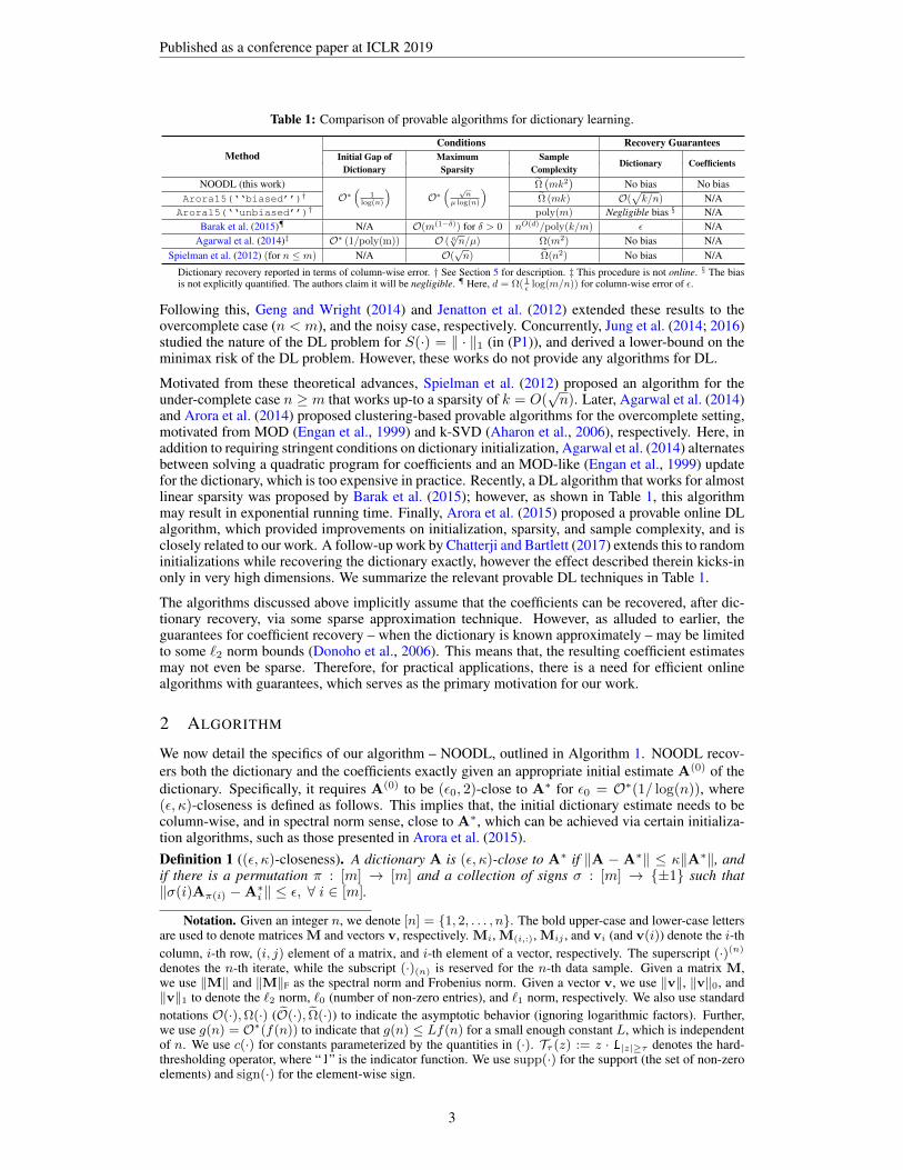
Table 1: Comparison of provable algorithms for dictionary learning.

MethodConditions Recovery Guarantees

Initial Gap of Maximum SampleDictionary Coefficients

Dictionary Sparsity ComplexityNOODL (this work)

O∗(

1log(n)

)O∗( √

nµ log(n)

) Ω(mk2

)No bias No bias

Arora15(‘‘biased’’)† Ω (mk) O(√k/n) N/A

Arora15(‘‘unbiased’’)† poly(m) Negligible bias § N/ABarak et al. (2015)¶ N/A O(m(1−δ)) for δ > 0 nO(d)/poly(k/m) ε N/A

Agarwal et al. (2014)‡ O∗ (1/poly(m)) O ( 6√n/µ) Ω(m2) No bias N/A

Spielman et al. (2012) (for n ≤ m) N/A O(√n) Ω(n2) No bias N/A

Dictionary recovery reported in terms of column-wise error. † See Section 5 for description. ‡ This procedure is not online. § The biasis not explicitly quantified. The authors claim it will be negligible. ¶ Here, d = Ω( 1

ε log(m/n)) for column-wise error of ε.

Following this, Geng and Wright (2014) and Jenatton et al. (2012) extended these results to theovercomplete case (n < m), and the noisy case, respectively. Concurrently, Jung et al. (2014; 2016)studied the nature of the DL problem for S(·) = ‖ · ‖1 (in (P1)), and derived a lower-bound on theminimax risk of the DL problem. However, these works do not provide any algorithms for DL.

Motivated from these theoretical advances, Spielman et al. (2012) proposed an algorithm for theunder-complete case n ≥ m that works up-to a sparsity of k = O(

√n). Later, Agarwal et al. (2014)

and Arora et al. (2014) proposed clustering-based provable algorithms for the overcomplete setting,motivated from MOD (Engan et al., 1999) and k-SVD (Aharon et al., 2006), respectively. Here, inaddition to requiring stringent conditions on dictionary initialization, Agarwal et al. (2014) alternatesbetween solving a quadratic program for coefficients and an MOD-like (Engan et al., 1999) updatefor the dictionary, which is too expensive in practice. Recently, a DL algorithm that works for almostlinear sparsity was proposed by Barak et al. (2015); however, as shown in Table 1, this algorithmmay result in exponential running time. Finally, Arora et al. (2015) proposed a provable online DLalgorithm, which provided improvements on initialization, sparsity, and sample complexity, and isclosely related to our work. A follow-up work by Chatterji and Bartlett (2017) extends this to randominitializations while recovering the dictionary exactly, however the effect described therein kicks-inonly in very high dimensions. We summarize the relevant provable DL techniques in Table 1.

The algorithms discussed above implicitly assume that the coefficients can be recovered, after dic-tionary recovery, via some sparse approximation technique. However, as alluded to earlier, theguarantees for coefficient recovery – when the dictionary is known approximately – may be limitedto some `2 norm bounds (Donoho et al., 2006). This means that, the resulting coefficient estimatesmay not even be sparse. Therefore, for practical applications, there is a need for efficient onlinealgorithms with guarantees, which serves as the primary motivation for our work.

2 ALGORITHM

We now detail the specifics of our algorithm – NOODL, outlined in Algorithm 1. NOODL recov-ers both the dictionary and the coefficients exactly given an appropriate initial estimate A(0) of thedictionary. Specifically, it requires A(0) to be (ε0, 2)-close to A∗ for ε0 = O∗(1/ log(n)), where(ε, κ)-closeness is defined as follows. This implies that, the initial dictionary estimate needs to becolumn-wise, and in spectral norm sense, close to A∗, which can be achieved via certain initializa-tion algorithms, such as those presented in Arora et al. (2015).Definition 1 ((ε, κ)-closeness). A dictionary A is (ε, κ)-close to A∗ if ‖A −A∗‖ ≤ κ‖A∗‖, andif there is a permutation π : [m] → [m] and a collection of signs σ : [m] → ±1 such that‖σ(i)Aπ(i) −A∗i ‖ ≤ ε, ∀ i ∈ [m].

Notation. Given an integer n, we denote [n] = 1, 2, . . . , n. The bold upper-case and lower-case lettersare used to denote matrices M and vectors v, respectively. Mi, M(i,:), Mij , and vi (and v(i)) denote the i-thcolumn, i-th row, (i, j) element of a matrix, and i-th element of a vector, respectively. The superscript (·)(n)denotes the n-th iterate, while the subscript (·)(n) is reserved for the n-th data sample. Given a matrix M,we use ‖M‖ and ‖M‖F as the spectral norm and Frobenius norm. Given a vector v, we use ‖v‖, ‖v‖0, and‖v‖1 to denote the `2 norm, `0 (number of non-zero entries), and `1 norm, respectively. We also use standardnotations O(·),Ω(·) (O(·), Ω(·)) to indicate the asymptotic behavior (ignoring logarithmic factors). Further,we use g(n) = O∗(f(n)) to indicate that g(n) ≤ Lf(n) for a small enough constant L, which is independentof n. We use c(·) for constants parameterized by the quantities in (·). Tτ (z) := z · 1|z|≥τ denotes the hard-thresholding operator, where “1” is the indicator function. We use supp(·) for the support (the set of non-zeroelements) and sign(·) for the element-wise sign.

3


Algorithm 1: NOODL: Neurally plausible alternating Optimization-based Online Dictionary Learning.

Input: Fresh data samples y(j) ∈ Rn for j ∈ [p] at each iteration t generated as per (1), where|x∗i | ≥ C for i ∈ supp(x∗). Parameters ηA, η(r)

x and τ (r) chosen as per A.5 and A.6. No. ofiterations T = Ω(log(1/εT )) and R = Ω(log(1/δR)), for target tolerances εT and δR.

Output: The dictionary A(t) and coefficient estimates x(t)(j) for j ∈ [p] at each iterate t.

Initialize: Estimate A(0), which is (ε0, 2)-near to A∗ for ε0 = O∗(1/ log(n))for t = 0 to T − 1 do

Predict: (Estimate Coefficients)for j = 1 to p do

Initialize: x(0)(j) = TC/2(A(t)>y(j)) (3)

for r = 0 to R− 1 do

Update: x(r+1)(j) = Tτ(r)(x

(r)(j) − η

(r)x A(t)>(A(t)x

(r)(j) − y(j))) (4)

endendx

(t)(j) := x

(R)(j) for j ∈ [p]

Learn: (Update Dictionary)Form empirical gradient estimate: g(t) = 1

p

∑pj=1(A(t)x

(t)(j) − y(j))sign(x

(t)(j))> (5)

Take a gradient descent step: A(t+1) = A(t) − ηA g(t) (6)

Normalize: A(t+1)i = A

(t+1)i /‖A(t+1)

i ‖ ∀ i ∈ [m]end

Due to the streaming nature of the incoming data, NOODL takes a mini-batch of p data samples atthe t-th iteration of the algorithm, as shown in Algorithm 1. It then proceeds by alternating betweentwo update stages: coefficient estimation (“Predict”) and dictionary update (“Learn”) as follows.

Predict Stage: For a general data sample y = A∗x∗, the algorithm begins by forming an initialcoefficient estimate x(0) based on a hard thresholding (HT) step as shown in (3), where Tτ (z) := z ·1|z|≥τ for a vector z. Given this initial estimate x(0), the algorithm iterates over R = Ω(log(1/δR))

IHT-based steps (4) to achieve a target tolerance of δR, such that (1− ηx)R ≤ δR. Here, η(r)x is the

learning rate, and τ (r) is the threshold at the r-th iterate of the IHT. In practice, these can be fixedto some constants for all iterations; see A.6 for details. Finally at the end of this stage, we haveestimate x(t) := x(R) of x∗.

Learn Stage: Using this estimate of the coefficients, we update the dictionary at t-th iteration A(t)

by an approximate gradient descent step (6), using the empirical gradient estimate (5) and the learn-ing rate ηA = Θ(m/k); see also A.5. Finally, we normalize the columns of the dictionary and con-tinue to the next batch. The running time of each step t of NOODL is thereforeO(mnp log(1/δR)).For a target tolerance of εT and δT , such that ‖A(T )

i −A∗i ‖ ≤ εT ,∀i ∈ [m] and |x(T )i − x∗i | ≤ δT

we choose T = max(Ω(log(1/εT )),Ω(log(√k/δT ))).

NOODL uses an initial HT step and an approximate gradient descent-based strategy as in Aroraet al. (2015). Following which, our IHT-based coefficient update step yields an estimate of thecoefficients at each iteration of the online algorithm. Coupled with the guaranteed progress made onthe dictionary, this also removes the bias in dictionary estimation. Further, the simultaneous recoveryof both factors also avoids an often expensive post-processing step for recovery of the coefficients.

3 MAIN RESULT

We start by introducing a few important definitions. First, as discussed in the previous section werequire that the initial estimate A(0) of the dictionary is (ε0, 2)-close to A∗. In fact, we require thiscloseness property to hold at each subsequent iteration t, which is a key ingredient in our analysis.This initialization achieves two goals. First, the ‖σ(i)Aπ(i) − A∗i ‖ ≤ ε0 condition ensures thatthe signed-support of the coefficients are recovered correctly (with high probability) by the hardthresholding-based coefficient initialization step, where signed-support is defined as follows.

4


Definition 2. The signed-support of a vector x is defined as sign(x) · supp(x).

Next, the ‖A−A∗‖ ≤ 2‖A∗‖ condition keeps the dictionary estimates close to A∗ and is used in ouranalysis to ensure that the gradient direction (5) makes progress. Further, in our analysis, we ensureεt (defined as ‖A(t)

i −A∗i ‖ ≤ εt) contracts at every iteration, and assume ε0, εt = O∗(1/ log(n)).Also, we assume that the dictionary A is fixed (deterministic) and µ-incoherent, defined as follows.

Definition 3. A matrix A ∈ Rn×m with unit-norm columns is µ-incoherent if for all i 6= j theinner-product between the columns of the matrix follow |〈Ai,Aj〉| ≤ µ/

√n.

The incoherence parameter measures the degree of closeness of the dictionary elements. Smallervalues (i.e., close to 0) of µ are preferred, since they indicate that the dictionary elements do notresemble each other. This helps us to effectively tell dictionary elements apart (Donoho and Huo,2001; Candes and Romberg, 2007). We assume that µ = O(log(n)) (Donoho and Huo, 2001). Next,we assume that the coefficients are drawn from a distribution class D defined as follows.

Definition 4 (Distribution class D). The coefficient vector x∗ belongs to an unknown distributionD, where the support S = supp(x∗) is at most of size k, Pr[i ∈ S] = Θ(k/m) and Pr[i, j ∈ S] =

Θ(k2/m2). Moreover, the distribution is normalized such that E[x∗i |i ∈ S] = 0 and E[x∗2

i |i ∈S] = 1, and when i ∈ S, |x∗i | ≥ C for some constant C ≤ 1. In addition, the non-zero entries aresub-Gaussian and pairwise independent conditioned on the support.

The randomness of the coefficient is necessary for our finite sample analysis of the convergence.Here, there are two sources of randomness. The first is the randomness of the support, where thenon-zero elements are assumed to pair-wise independent. The second is the value an element inthe support takes, which is assumed to be zero mean with variance one, and bounded in magnitude.Similar conditions are also required for support recovery of sparse coefficients, even when the dic-tionary is known (Wainwright, 2009; Yuan et al., 2016). Note that, although we only consider thecase |x∗i | ≥ C for ease of discussion, analogous results may hold more generally for x∗i s drawnfrom a distribution with sufficiently (exponentially) small probability of taking values in [−C,C].

Recall that, given the coefficients, we recover the dictionary by making progress on the least squaresobjective (P1) (ignoring the term penalizing S(·)). Note that, our algorithm is based on findingan appropriate direction to ensure descent based on the geometry of the objective. To this end, weadopt a gradient descent-based strategy for dictionary update. However, since the coefficients are notexactly known, this results in an approximate gradient descent-based approach, where the empiricalgradient estimate is formed as (5). In our analysis, we establish the conditions under which boththe empirical gradient vector (corresponding to each dictionary element) and the gradient matrixconcentrate around their means. To ensure progress at each iterate t, we show that the expectedgradient vector is (Ω(k/m),Ω(m/k), 0)-correlated with the descent direction, defined as follows.

Definition 5. A vector g(t) is (ρ−, ρ+ , ζt)-correlated with a vector z∗ if

〈g(t), z(t) − z∗〉 ≥ ρ−‖z(t) − z∗‖2 + ρ+‖g(t)‖2 − ζt.

This can be viewed as a local descent condition which leads to the true dictionary columns; see alsoCandes et al. (2015), Chen and Wainwright (2015) and Arora et al. (2015). In convex optimiza-tion literature, this condition is implied by the 2ρ−-strong convexity, and 1/2ρ+ -smoothness of theobjective. We show that for NOODL, ζt = 0, which facilitates linear convergence to A∗ withoutincurring any bias. Overall our specific model assumptions for the analysis can be formalized as:

A.1 A∗ is µ-incoherent (Def. 3), where µ = O(log(n)), ‖A∗‖ = O(√m/n) and m = O(n);

A.2 The coefficients are drawn from the distribution class D, as per Def. 4;A.3 The sparsity k satisfies k = O∗(

√n/µ log(n));

A.4 A(0) is (ε0, 2)-close to A∗ as per Def. 1, and ε0 = O∗(1/ log(n));A.5 The step-size for dictionary update satisfies ηA = Θ(m/k);

A.6 The step-size and threshold for coefficient estimation satisfies η(r)x < c1(εt, µ, n, k) =

Ω(k/√n) < 1 and τ (r) = c2(εt, µ, k, n) = Ω(k2/n) for small constants c1 and c2.

We are now ready to state our main result. A summary of the notation followed by a details of theanalysis is provided in Appendix A and Appendix B, respectively.

5


Theorem 1 (Main Result). Suppose that assumptions A.1-A.6 hold, and Algorithm 1 is providedwith p = Ω(mk2) new samples generated according to model (1) at each iteration t. Then, withprobability at least (1 − δ(t)

alg ) for some small constant δ(t)alg , given R = Ω(log(n)), the coefficient

estimate x(t)i at t-th iteration has the correct signed-support and satisfies

(x(t)i − x∗i )

2 = O(k(1− ω)t/2‖A(0)i −A∗i ‖), for all i ∈ supp(x∗).

Furthermore, for some 0 < ω < 1/2, the estimate A(t) at (t)-th iteration satisfies

‖A(t)i −A∗i ‖2 ≤ (1− ω)t‖A(0)

i −A∗i ‖2, for all t = 1, 2, . . . ..

Our main result establishes that when the model satisfies A.1∼A.3, the errors corresponding to thedictionary and coefficients geometrically decrease to the true model parameters, given appropriatedictionary initialization and learning parameters (step sizes and threshold); see A.4∼A.6. In otherwords, to attain a target tolerance of εT and δT , where ‖A(T )

i − A∗i ‖ ≤ εT , |x(T )i − x∗i | ≤ δT ,

we require T = max(Ω(log(1/εT )),Ω(log(√k/δT ))) outer iterations and R = Ω(log(1/δR)) IHT

steps per outer iteration. Here, δR ≥ (1 − ηx)R is the target decay tolerance for the IHT steps.An appropriate number of IHT steps, R, remove the dependence of final coefficient error (per outeriteration) on the initial x(0). In Arora et al. (2015), this dependence in fact results in an irreducibleerror, which is the source of bias in dictionary estimation. As a result, since (for NOODL) the errorin the coefficients only depends on the error in the dictionary, it can be made arbitrarily small, at ageometric rate, by the choice of εT , δT , and δR. Also, note that, NOODL can tolerate i.i.d. noise, aslong as the noise variance is controlled to enable the concentration results to hold; we consider thenoiseless case here for ease of discussion, which is already highly involved.

Intuitively, Theorem 1 highlights the symbiotic relationship between the two factors. It shows that,to make progress on one, it is imperative to make progress on the other. The primary conditionthat allows us to make progress on both factors is the signed-support recovery (Def. 2). However,the introduction of IHT step adds complexity in the analysis of both the dictionary and coefficients.To analyze the coefficients, in addition to deriving conditions on the parameters to preserve thecorrect signed-support, we analyze the recursive IHT update step, and decompose the noise terminto a component that depends on the error in the dictionary, and the other that depends on the initialcoefficient estimate. For the dictionary update, we analyze the interactions between elements of thecoefficient vector (introduces by the IHT-based update step) and show that the gradient vector forthe dictionary update is (Ω(k/m),Ω(m/k), 0)-correlated with the descent direction. In the end, thisleads to exact recovery of the coefficients and removal of bias in the dictionary estimation. Note thatour analysis pipeline is standard for the convergence analysis for iterative algorithms. However, theintroduction of the IHT-based strategy for coefficient update makes the analysis highly involved ascompared to existing results, e.g., the simple HT-based coefficient estimate in Arora et al. (2015).

NOODL has an overall running time ofO(mnp log(1/δR) max(log(1/εT ), log(√k/δT )) to achieve

target tolerances εT and δT , with a total sample complexity of p·T = Ω(mk2). Thus to remove bias,the IHT-based coefficient update introduces a factor of log(1/δR) in the computational complexityas compared to Arora et al. (2015) (has a total sample complexity of p · T = Ω(mk)), and also doesnot have the exponential running time and sample complexity as Barak et al. (2015); see Table 1.

4 NEURAL IMPLEMENTATION OF NOODL

The neural plausibility of our algorithm implies that it can be implemented as a neural network.This is because, NOODL employs simple linear and non-linear operations (such as inner-productand hard-thresholding) and the coefficient updates are separable across data samples, as shown in(4) of Algorithm 1. To this end, we present a neural implementation of our algorithm in Fig. 1,which showcases the applicability of NOODL in large-scale distributed learning tasks, motivatedfrom the implementations described in (Olshausen and Field, 1997) and (Arora et al., 2015).

The neural architecture shown in Fig. 1(a) has three layers – input layer, weighted residual evaluationlayer, and the output layer. The input to the network is a data and step-size pair (y(j), ηx) to eachinput node. Given an input, the second layer evaluates the weighted residuals as shown in Fig. 1.Finally, the output layer neurons evaluate the IHT iterates x(r+1)

(j) (4). We illustrate the operation ofthis architecture using the timing diagram in Fig. 1(b). The main stages of operation are as follows.

6


(a) Neural implementation of NOODL

Figure 1: A neural implementation ofNOODL. Panel (a) shows the neural architec-ture, which consists of three layers: an in-put layer, a weighted residual evaluation layer(evaluates ηx

(y(j) − A(t)x

(r)

(j)

)), and an out-

put layer. Panel (b) shows the operation of theneural architecture in panel (a). The update ofx(r+1)

(j) is given by (4).

` = 0 ` = 1 ` = 2 ` = 3 ` = 4 ` = 5 . . . ` = 2R+ 1 HebbianLearning:Residualsharing anddictionaryupdate.

Output: x← 0 0 x(0)

(j) = Tτ (A(t)>y(j)) x(0)

(j) x(1)

(j) x(1)

(j) . . . x(R)

(j)

Residual: 0 y(j) y(j) ηx(y(j) −A(t)x(0)

(j)) ηx(y(j) −A(t)x(0)

(j)) ηx(y(j) −A(t)x(1)

(j)) . . . ηx(y(j) −A(t)x(R−1)

(j) )

Input: (y(j), 1) . (y(j), ηx) . . . . . . (y(j), 1)

(b) The timing sequence of the neural implementation.

Initial Hard Thresholding Phase: The coefficients initialized to zero, and an input (y(j), 1) isprovided to the input layer at a time instant ` = 0, which communicates these to the second layer.Therefore, the residual at the output of the weighted residual evaluation layer evaluates to y(j) at` = 1. Next, at ` = 2, this residual is communicated to the output layer, which results in evaluationof the initialization x

(0)(j) as per (3). This iterate is communicated to the second layer for the next

residual evaluation. Also, at this time, the input layer is injected with (y(j), ηx) to set the step sizeparameter ηx for the IHT phase, as shown in Fig. 1(b).

Iterative Hard Thresholding (IHT) Phase: Beginning ` = 3, the timing sequence enters theIHT phase. Here, the output layer neurons communicate the iterates x(r+1)

(j) to the second layer forevaluation of subsequent iterates as shown in Fig. 1(b). The process then continues till the timeinstance ` = 2R + 1, for R = Ω(log(1/δR)) to generate the final coefficient estimate x

(t)(j) := x

(R)(j)

for the current batch of data. At this time, the input layer is again injected with (y(j), 1) to preparethe network for residual sharing and gradient evaluation for dictionary update.

Dictionary Update Phase: The procedure now enters the dictionary update phase, denoted as “Heb-bian Learning” in the timing sequence. In this phase, each output layer neuron communicates thefinal coefficient estimate x

(t)(j) = x

(R)(j) to the second layer, which evaluates the residual for one last

time (with ηx = 1), and shares it across all second layer neurons (“Hebbian learning”). This allowseach second layer neuron to evaluate the empirical gradient estimate (5), which is used to updatethe current dictionary estimate (stored as weights) via an approximate gradient descent step. Thiscompletes one outer iteration of Algorithm 1, and the process continues for T iterations to achievetarget tolerances εT and δT , with each step receiving a new mini-batch of data.

5 EXPERIMENTS

We now analyze the convergence properties and sample complexity of NOODL via experimentalevaluations 2. The experimental data generation set-up, additional results, including analysis ofcomputational time, are shown in Appendix E.

5.1 CONVERGENCE ANALYSIS

We compare the performance of our algorithm NOODL with the current state-of-the-art alternatingoptimization-based online algorithms presented in Arora et al. (2015), and the popular algorithm pre-sented in Mairal et al. (2009) (denoted as Mairal ‘09). First of these, Arora15(‘‘biased’’),is a simple neurally plausible method which incurs a bias and has a sample complexity of Ω(mk).The other, referred to as Arora15(‘‘unbiased’’), incurs no bias as per Arora et al. (2015),but the sample complexity results were not established.

Discussion: Fig. 2 panels (a-i), (b-i), (c-i), and (d-i) show the performance of the aforementionedmethods for k = 10, 20, 50, and 100, respectively. Here, for all experiments we set ηx = 0.2 andτ = 0.1. We terminate NOODL when the error in dictionary is less than 10−10. Also, for coefficientupdate, we terminate when change in the iterates is below 10−12. For k = 10, 20 and k = 50,

2The associated code is made available at https://github.com/srambhatla/NOODL.

7


k = 10, ηA = 30 k = 20, ηA = 30 k = 50, ηA = 15 k = 100, ηA = 15 Phase Transition

Dic

tiona

ryR

ecov

ery

Acr

ossT

echn

ique

s

50 100 150Iterations

10-10

10-8

10-6

10-4

10-2

Rel

ativ

e F

robe

nius

Err

or20 40 60 80 100

Iterations

10-10

10-8

10-6

10-4

10-2

20 40 60 80Iterations

10-10

10-8

10-6

10-4

10-2


10-10

10-8

10-6

10-4

10-2

100

0 0.5 1 1.5 2p=m

0

0.2

0.4

0.6

0.8

1

Suc

cess

Pro

babi

lity

m = nm = 2nm = 4n

(a-i) (b-i) (c-i) (d-i) (e-i) Dictionary

Perf

orm

ance

ofN

OO

DL

50 100 150Iterations

10-10

10-8

10-6

10-4

10-2

Rel

ativ

e F

robe

nius

Err

or

20 40 60 80 100Iterations

10-10

10-8

10-6

10-4

10-2

Rel

ativ

e Fr

oben

ius

Erro

r20 40 60 80

Iterations

10-10

10-8

10-6

10-4

10-2

Rel

ativ

e Fr

oben

ius

Erro

r


10-10

10-8

10-6

10-4

10-2

Rel

ativ

e Fr

oben

ius

Erro

r

0 0.5 1 1.5 2p=m

0

0.2

0.4

0.6

0.8

1

Suc

cess

Pro

babi

lity

m = nm = 2nm = 4n

(a-ii) (b-ii) (c-ii) (d-ii) (e-ii) Coefficients

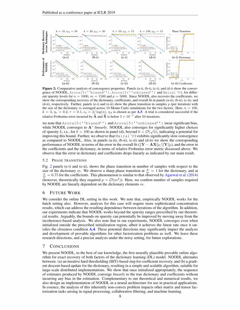
Figure 2: Comparative analysis of convergence properties. Panels (a-i), (b-i), (c-i), and (d-i) show the conver-gence of NOODL, Arora15(‘‘biased’’), Arora15(‘‘unbiased’’) and Mairal ‘09, for differ-ent sparsity levels for n = 1000, m = 1500 and p = 5000. Since NOODL also recovers the coefficients, weshow the corresponding recovery of the dictionary, coefficients, and overall fit in panels (a-ii), (b-ii), (c-ii), and(d-ii), respectively. Further, panels (e-i) and (e-ii) show the phase transition in samples p (per iteration) withthe size of the dictionary m averaged across 10 Monte Carlo simulations for the two factors. Here, n = 100,k = 3, ηx = 0.2, τ = 0.1, ε0 = 2/ log(n), ηA is chosen as per A.5. A trial is considered successful if therelative Frobenius error incurred by A and X is below 5× 10−7 after 50 iterations.

we note that Arora15(‘‘biased’’) and Arora15(‘‘unbiased’’) incur significant bias,while NOODL converges to A∗ linearly. NOODL also converges for significantly higher choicesof sparsity k, i.e., for k = 100 as shown in panel (d), beyond k = O(

√n), indicating a potential for

improving this bound. Further, we observe that Mairal ‘09 exhibits significantly slow convergenceas compared to NOODL. Also, in panels (a-ii), (b-ii), (c-ii) and (d-ii) we show the correspondingperformance of NOODL in terms of the error in the overall fit (‖Y −AX‖F/‖Y‖F), and the error inthe coefficients and the dictionary, in terms of relative Frobenius error metric discussed above. Weobserve that the error in dictionary and coefficients drops linearly as indicated by our main result.

5.2 PHASE TRANSITIONS

Fig. 2 panels (e-i) and (e-ii), shows the phase transition in number of samples with respect to thesize of the dictionary m. We observe a sharp phase transition at p

m = 1 for the dictionary, and atpm = 0.75 for the coefficients. This phenomenon is similar to that observed by Agarwal et al. (2014)(however, theoretically they required p = O(m2)). Here, we confirm number of samples requiredby NOODL are linearly dependent on the dictionary elements m.

6 FUTURE WORK

We consider the online DL setting in this work. We note that, empirically NOODL works for thebatch setting also. However, analysis for this case will require more sophisticated concentrationresults, which can address the resulting dependence between iterations of the algorithm. In addition,our experiments indicate that NOODL works beyond the sparsity ranges prescribed by our theoreti-cal results. Arguably, the bounds on sparsity can potentially be improved by moving away from theincoherence-based analysis. We also note that in our experiments, NOODL converges even wheninitialized outside the prescribed initialization region, albeit it achieves the linear rate once it sat-isfies the closeness condition A.4. These potential directions may significantly impact the analysisand development of provable algorithms for other factorization problems as well. We leave theseresearch directions, and a precise analysis under the noisy setting, for future explorations.

7 CONCLUSIONS

We present NOODL, to the best of our knowledge, the first neurally plausible provable online algo-rithm for exact recovery of both factors of the dictionary learning (DL) model. NOODL alternatesbetween: (a) an iterative hard thresholding (IHT)-based step for coefficient recovery, and (b) a gradi-ent descent-based update for the dictionary, resulting in a simple and scalable algorithm, suitable forlarge-scale distributed implementations. We show that once initialized appropriately, the sequenceof estimates produced by NOODL converge linearly to the true dictionary and coefficients withoutincurring any bias in the estimation. Complementary to our theoretical and numerical results, wealso design an implementation of NOODL in a neural architecture for use in practical applications.In essence, the analysis of this inherently non-convex problem impacts other matrix and tensor fac-torization tasks arising in signal processing, collaborative filtering, and machine learning.

8


ACKNOWLEDGMENT

The authors would like to graciously acknowledge support from DARPA Young Faculty Award,Grant No. N66001-14-1-4047.

REFERENCES

AGARWAL, A., ANANDKUMAR, A., JAIN, P., NETRAPALLI, P. and TANDON, R. (2014). Learningsparsely used overcomplete dictionaries. In Conference on Learning Theory (COLT).

AHARON, M., ELAD, M. and BRUCKSTEIN, A. (2006). k-svd: An algorithm for designing over-complete dictionaries for sparse representation. IEEE Transactions on Signal Processing, 544311–4322.

ARORA, S., GE, R., MA, T. and MOITRA, A. (2015). Simple, efficient, and neural algorithms forsparse coding. In Conference on Learning Theory (COLT).

ARORA, S., GE, R. and MOITRA, A. (2014). New algorithms for learning incoherent and over-complete dictionaries. In Conference on Learning Theory (COLT).

BARAK, B., KELNER, J. A. and STEURER, D. (2015). Dictionary learning and tensor decompo-sition via the sum-of-squares method. In Proceedings of the 47th annual ACM symposium onTheory of Computing. ACM.

BECK, A. and TEBOULLE, M. (2009). A fast iterative shrinkage-thresholding algorithm for linearinverse problems. SIAM Journal on Imaging Sciences, 2 183–202.

BLUMENSATH, T. and DAVIES, M. E. (2009). Iterative hard thresholding for compressed sensing.Applied and Computational Harmonic Analysis, 27 265–274.

CANDES, E. and ROMBERG, J. (2007). Sparsity and incoherence in compressive sampling. InverseProblems, 23 969.

CANDES, E. J., LI, X. and SOLTANOLKOTABI, M. (2015). Phase retrieval via wirtinger flow:Theory and algorithms. IEEE Transactions on Information Theory, 61 1985–2007.

CHATTERJI, N. and BARTLETT, P. L. (2017). Alternating minimization for dictionary learning withrandom initialization. In Advances in Neural Information Processing Systems.

CHEN, S. S., DONOHO, D. L. and SAUNDERS, M. A. (1998). Atomic decomposition by basispursuit. SIAM Journal on Scientific Computing, 20 33–61.

CHEN, Y. and WAINWRIGHT, M. J. (2015). Fast low-rank estimation by projected gradient descent:General statistical and algorithmic guarantees. CoRR, abs/1509.03025.

DONOHO, D., ELAD, M. and TEMLYAKOV, V. N. (2006). Stable recovery of sparse overcompleterepresentations in the presence of noise. IEEE Transactions on Information Theory, 52 6–18.

DONOHO, D. L. and HUO, X. (2001). Uncertainty principles and ideal atomic decomposition.IEEE Transactions on Information Theory, 47 2845–2862.

ELAD, M. (2010). Sparse and Redundant Representations: From Theory to Applications in Signaland Image Processing. 1st ed. Springer Publishing Company, Incorporated.

ELAD, M. and AHARON, M. (2006). Image denoising via sparse and redundant representationsover learned dictionaries. IEEE Transactions on Image Processing, 15 3736–3745.

ENGAN, K., AASE, S. O. and HUSOY, J. H. (1999). Method of optimal directions for frame design.In IEEE International Conference on Acoustics, Speech, and Signal Processing (ICASSP), vol. 5.IEEE.

FULLER, W. A. (2009). Measurement error models, vol. 305. John Wiley & Sons.

GENG, Q. and WRIGHT, J. (2014). On the local correctness of `1-minimization for dictionarylearning. In 2014 IEEE International Symposium on Information Theory (ISIT). IEEE.

GERSHGORIN, S. A. (1931). Uber die abgrenzung der eigenwerte einer matrix 749–754.

9


GREGOR, K. and LECUN, Y. (2010). Learning fast approximations of sparse coding. In Proceed-ings of the 27th International Conference on Machine Learning (ICML). Omnipress.

GRIBONVAL, R. and SCHNASS, K. (2010). Dictionary identification and sparse matrix-factorizationvia `1 -minimization. IEEE Transactions on Information Theory, 56 3523–3539.

HANSON, D. and WRIGHT, F. T. (1971). A bound on tail probabilities for quadratic forms inindependent random variables. The Annals of Mathematical Statistics, 42 1079–1083.

HAUPT, J. and NOWAK, R. (2006). Signal reconstruction from noisy random projections. IEEETransactions on Information Theory, 52 4036–4048.

JENATTON, R., GRIBONVAL, R. and BACH, F. (2012). Local stability and robustness of sparsedictionary learning in the presence of noise. Research report.https://hal.inria.fr/hal-00737152

JUNG, A., ELDAR, Y. and GORTZ, N. (2014). Performance limits of dictionary learning for sparsecoding. In Proceedings of the European Signal Processing Conference (EUSIPCO),. IEEE.

JUNG, A., ELDAR, Y. C. and GRTZ, N. (2016). On the minimax risk of dictionary learning. IEEETransactions on Information Theory, 62 1501–1515.

KREUTZ-DELGADO, K., MURRAY, J. F., RAO, B. D., ENGAN, K., LEE, T. and SEJNOWSKI,T. J. (2003). Dictionary learning algorithms for sparse representation. Neural Computation, 15349–396.

LEE, H., BATTLE, A., RAINA, R. and NG, A. Y. (2007). Efficient sparse coding algorithms. InAdvances in Neural Information Processing Systems (NIPS.

LEWICKI, M. S. and SEJNOWSKI, T. J. (2000). Learning overcomplete representations. NeuralComputation, 12 337–365.

LI, X., WANG, Z., LU, J., ARORA, R., HAUPT, J., LIU, H. and ZHAO, T. (2016a). Sym-metry, saddle points, and global geometry of nonconvex matrix factorization. arXiv preprintarXiv:1612.09296.

LI, X., ZHAO, T., ARORA, R., LIU, H. and HAUPT, J. (2016b). Stochastic variance reducedoptimization for nonconvex sparse learning. In International Conference on Machine Learning.

MAIRAL, J., BACH, F., PONCE, J. and SAPIRO, G. (2009). Online dictionary learning for sparsecoding. In Proceedings of the International Conference on Machine Learning (ICML). ACM.

MALLAT, S. G. and ZHANG, Z. (1993). Matching pursuits with time-frequency dictionaries. IEEETransactions on Signal Processing, 41 3397–3415.

OLSHAUSEN, B. A. and FIELD, D. J. (1997). Sparse coding with an overcomplete basis set: Astrategy employed by v1? Vision Research, 37 3311–3325.

PEARSON, K. (1901). On lines and planes of closest fit to systems of points in space. The London,Edinburgh, and Dublin Philosophical Magazine and Journal of Science, 2 559–572.https://doi.org/10.1080/14786440109462720

RAMBHATLA, S. and HAUPT, J. (2013). Semi-blind source separation via sparse representationsand online dictionary learning. In 2013 Asilomar Conference on Signals, Systems and Computers,.IEEE.

RAMBHATLA, S., LI, X. and HAUPT, J. (2016). A dictionary based generalization of robust PCA.In IEEE Global Conference on Signal and Information Processing (GlobalSIP). IEEE.

RAMBHATLA, S., LI, X. and HAUPT, J. (2017). Target-based hyperspectral demixing via general-ized robust PCA. In 51st Asilomar Conference on Signals, Systems, and Computers. IEEE.https://doi.org/10.1109/ACSSC.2017.8335372

RAMBHATLA, S., LI, X., REN, J. and HAUPT, J. (2019a). A dictionary-based generalization ofrobust PCA part I: Study of theoretical properties. abs/1902.08304.https://arxiv.org/abs/1902.08304

10

https://hal.inria.fr/hal-00737152

https://doi.org/10.1080/14786440109462720

https://doi.org/10.1109/ACSSC.2017.8335372

https://arxiv.org/abs/1902.08304


RAMBHATLA, S., LI, X., REN, J. and HAUPT, J. (2019b). A dictionary-based generalization ofrobust PCA part II: Applications to hyperspectral demixing. abs/1902.10238.https://arxiv.org/abs/1902.10238

RAMIREZ, I., SPRECHMANN, P. and SAPIRO, G. (2010). Classification and clustering via dictio-nary learning with structured incoherence and shared features. In IEEE Conference on ComputerVision and Pattern Recognition (CVPR). IEEE.

RANZATO, M., BOUREAU, Y. and LECUN, Y. (2008). Sparse feature learning for deep beliefnetworks. In Advances in Neural Information Processing Systems (NIPS). 1185–1192.

RUDELSON, M. and VERSHYNIN, R. (2013). Hanson-wright inequality and sub-gaussian concen-tration. Electronic Communications in Probability, 18.

SPIELMAN, D. A., WANG, H. and WRIGHT, J. (2012). Exact recovery of sparsely-used dictionar-ies. In Conference on Learning Theory (COLT).

TIBSHIRANI, R. (1996). Regression shrinkage and selection via the lasso. Journal of the RoyalStatistical Society. Series B (Methodological) 267–288.

TROPP, J. (2015). An introduction to matrix concentration inequalities. Foundations and Trends inMachine Learning, 8 1–230.

WAINWRIGHT, M. J. (2009). Sharp thresholds for high-dimensional and noisy sparsity recoveryusing `1-constrained quadratic programming (lasso). IEEE Transactions on Information Theory,55 2183–2202.

YUAN, X., LI, P. and ZHANG, T. (2016). Exact recovery of hard thresholding pursuit. In Advancesin Neural Information Processing Systems (NIPS).

11

https://arxiv.org/abs/1902.10238


A SUMMARY OF NOTATION

We summarizes the definitions of some frequently used symbols in our analysis in Table 2. Inaddition, we use D(v) as a diagonal matrix with elements of a vector v on the diagonal. Given amatrix M, we use M−i to denote a resulting matrix without i-th column. Also note that, since weshow that ‖A(t)

i −A∗i ‖ ≤ εt contracts in every step, therefore we fix εt, ε0 = O∗(1/ log(n)) in ouranalysis.

Table 2: Frequently used symbols

Dictionary RelatedSymbol DefinitionA

(t)i i-th column of the dictionary estimate at the t-th iterate.εt ‖A(t)

i −A∗i ‖ ≤ εt = O∗( 1log(n) ) Upper-bound on column-wise error

at the t-th iterate.µt

µt√n

= µ√n

+ 2εt Incoherence between the columnsof A(t); See Claim 1.

λ(t)j λ

(t)j := |〈A(t)

j −A∗j ,A∗j 〉| ≤

ε2t2 Inner-product between the error and

the dictionary element.

Λ(t)S (i, j) Λ

(t)S (i, j) =

λ

(t)j , for j = i, i ∈ S

0, otherwise.A diagonal matrix of size |S| × |S|with λ(t)

j on the diagonal for j ∈ S.

Coefficient RelatedSymbol Definitionx

(r)i i-th element the coefficient estimate at the r-th IHT iterate.C |x∗i | ≥ C for i ∈ supp(x∗) and C ≤ 1 Lower-bound on x∗i s.S S := supp(x∗) where |S| ≤ k Support of x∗

δR δR := (1− ηx + ηxµt√n

)R ≥ (1− ηx)R Decay parameter for coefficients.

δT |x(T )i − x∗i | ≤ δT∀i ∈ supp(x∗) Target coefficient element error tol-

erance.C

(`)i C

(`)i := |x∗i − x

(`)i | for i ∈ supp(x∗) Error in non-zero elements of the

coefficient vector.

ProbabilitiesSymbol Definition Symbol Definitionqi qi = Pr[i ∈ S] = Θ( km ) qi,j qi,j = Pr[i, j ∈ S] = Θ( k

2

m2 )

pi pi = E[x∗i sign(x∗i )|x∗i 6= 0] δ(t)T δ

(t)T = 2m exp(−C2/O∗(ε2t ))

δ(t)β δ

(t)β = 2k exp(−1/O(εt)) δ

(t)HW δ

(t)HW = exp(−1/O(εt))

δ(t)gi δ

(t)gi = exp(−Ω(k)) δ

(t)g δ

(t)g = (n+m) exp(−Ω(m

√log(n))

Other termsSymbol Definitionξ

(r+1)j ξ

(r+1)j :=

∑i 6=j

(〈A(t)j −A∗j ,A

∗i 〉+ 〈A∗j ,A∗i 〉)x∗i −

∑i6=j〈A(t)

j ,A(t)i 〉x

(r)i

β(t)j β

(t)j :=

∑i6=j

(〈A∗j ,A∗i −A(t)i 〉+ 〈A∗j −A

(t)j ,A

(t)i 〉+ 〈A(t)

j −A∗j ,A∗i 〉)x∗i

tβ tβ = O(√kεt) is an upper-bound on β(t)

j with probability at least (1− δ(t)β )

ξ(r+1)j ξ

(r+1)j := β

(t)j +

∑i6=j|〈A(t)

j ,A(t)i 〉| |x∗i − x

(r)i |

∆(t)j ∆

(t)j := E[A

(t)S ϑ

(R)S sign(x∗j )]

ϑ(R)i ϑ

(R)i :=

R∑r=1

ηxξ(r)i (1− ηx)R−r + γ

(R)i

γ(R)i γ

(R)i := (1− ηx)R(x

(0)i − x∗i (1− λ

(t)i ))

γ γ := E[(A(t)x− y)sign(x∗j )1Fx∗]; See † below.

xi xi := x(R)i = x∗i (1− λ

(t)i ) + ϑ

(R)i

†1Fx∗ is the indicator function corresponding to the event that sign(x∗) = sign(x),denoted by Fx∗ , and similarly for the complement Fx∗

12


B PROOF OF THEOREM 1

We now prove our main result. The detailed proofs of intermediate lemmas and claims are organizedin Appendix C and Appendix D, respectively. Furthermore, the standard concentration results arestated in Appendix F for completeness. Also, see Table 3 for a map of dependence between theresults.

OVERVIEW

Given an (ε0, 2)-close estimate of the dictionary, the main property that allows us to make progresson the dictionary is the recovery of the correct sign and support of the coefficients. Therefore, wefirst show that the initial coefficient estimate (3) recovers the correct signed-support in Step I.A.Now, the IHT-based coefficient update step also needs to preserve the correct signed-support. Thisis to ensure that the approximate gradient descent-based update for the dictionary makes progress.Therefore, in Step I.B, we derive the conditions under which the signed-support recovery conditionis preserved by the IHT update.

To get a handle on the coefficients, in Step II.A, we derive an upper-bound on the error incurredby each non-zero element of the estimated coefficient vector, i.e., |xi − x∗i | for i ∈ S for a generalcoefficient vector x∗, and show that this error only depends on εt (the column-wise error in thedictionary) given enough IHT iterations R as per the chosen decay parameter δR. In addition, foranalysis of the dictionary update, we develop an expression for the estimated coefficient vector inStep II.B.

We then use the coefficient estimate to show that the gradient vector satisfies the local descent con-dition (Def. 5). This ensures that the gradient makes progress after taking the gradient descent-basedstep (6). To begin, we first develop an expression for the expected gradient vector (corresponding toeach dictionary element) in Step III.A. Here, we use the closeness property Def 1 of the dictionaryestimate. Further, since we use an empirical estimate, we show that the empirical gradient vectorconcentrates around its mean in Step III.B. Now using Lemma 15, we have that descent along thisdirection makes progress.

Next in Step IV.A and Step IV.B, we show that the updated dictionary estimate maintains the close-ness property Def 1. This sets the stage for the next dictionary update iteration. As a result, ourmain result establishes the conditions under which any t-th iteration succeeds.

Our main result is as follows.

Theorem 1 (Main Result) Suppose that assumptions A.1-A.6 hold, and Algorithm 1 is providedwith p = Ω(mk2) new samples generated according to model (1) at each iteration t. Then, withprobability at least (1 − δ(t)

alg ), given R = Ω(log(n)), the coefficient estimate x(t)i at t-th iteration

has the correct signed-support and satisfies

(x(t)i − x∗i )

2 = O(k(1− ω)t/2‖A(0)i −A∗i ‖), for all i ∈ supp(x∗).

Furthermore, for some 0 < ω < 1/2, the estimate A(t) at (t)-th iteration satisfies

‖A(t)i −A∗i ‖2 ≤ (1− ω)t‖A(0)

i −A∗i ‖2, for all t = 1, 2, . . . ..

Here, δ(t)alg is some small constant, where δ

(t)alg = δ

(t)T + δ

(t)β + δHW + δ

(t)gi + δ

(t)g , δ(t)

T =

2m exp(−C2/O∗(ε2t )), δ(t)β = 2k exp(−1/O(εt)), δ(t)

HW = exp(−1/O(εt)), δ(t)gi = exp(−Ω(k)),

δ(t)g = (n+m) exp(−Ω(m

√log(n)), and ‖A(t)

i −A∗i ‖ ≤ εt.

STEP I: COEFFICIENTS HAVE THE CORRECT SIGNED-SUPPORT

As a first step, we ensure that our coefficient estimate has the correct signed-support (Def. 2). Tothis end, we first show that the initialization has the correct signed-support, and then show thatthe iterative hard-thresholding (IHT)-based update step preserves the correct signed-support for asuitable choice of parameters.

13


• Step I.A: Showing that the initial coefficient estimate has the correct signed-support–Given an (ε0, 2)-close estimate A(0) of A∗, we first show that for a general sample y theinitialization step (3) recovers the correct signed-support with probability at least (1−δ(t)

T ),where δ(t)

T = 2m exp(− C2

O∗(ε2t )). This is encapsulated by the following lemma.

Lemma 1 (Signed-support recovery by coefficient initialization step). Suppose A(t)

is εt-close to A∗. Then, if µ = O(log(n)), k = O∗(√n/µ log(n)), and εt =

O∗(1/√

log(m)), with probability at least (1− δ(t)T ) for each random sample y = A∗x∗:

sign(TC/2((A(t))>y) = sign(x∗),

where δ(t)T = 2m exp(− C2

O∗(ε2t )).

Note that this result only requires the dictionary to be column-wise close to the true dictio-nary, and works for less stringent conditions on the initial dictionary estimate, i.e., requiresεt = O∗(1/

√log(m)) instead of εt = O∗(1/ log(m)); see also (Arora et al., 2015).

• Step I.B: The iterative IHT-type updates preserve the correct signed support– Next,we show that the IHT-type coefficient update step (4) preserves the correct signed-supportfor an appropriate choice of step-size parameter η(r)

x and threshold τ (r). The choice ofthese parameters arises from the analysis of the IHT-based update step. Specifically, weshow that at each iterate r, the step-size η(r)

x should be chosen to ensure that the componentcorresponding to the true coefficient value is greater than the “interference” introduced byother non-zero coefficient elements. Then, if the threshold is chosen to reject this “noise”,each iteration of the IHT-based update step preserves the correct signed-support.

Lemma 2 (IHT update step preserves the correct signed-support). Suppose A(t) is εt-close to A∗, µ = O(log(n)), k = O∗(

√n/µ log(n)), and εt = O∗(1/ log(m)) Then, with

probability at least (1 − δ(t)β − δ

(t)T ), each iterate of the IHT-based coefficient update step

shown in (4) has the correct signed-support, if for a constant c(r)1 (εt, µ, k, n) = Ω(k2/n),the step size is chosen as η(r)

x ≤ c(r)1 , and the threshold τ (r) is chosen as

τ (r) = η(r)x (tβ + µt√

n‖x(r−1) − x∗‖1) := c

(r)2 (εt, µ, k, n) = Ω(k2/n),

for some constants c1 and c2. Here, tβ = O(√kεt), δ(t)

T = 2m exp(− C2

O∗(ε2t )) ,and δ(t)

β =

2k exp(− 1O(εt)

).

Note that, although we have a dependence on the iterate r in choice of η(r)x and τ (r), these

can be set to some constants independent of r. In practice, this dependence allows forgreater flexibility in the choice of these parameters.

STEP II: ANALYZING THE COEFFICIENT ESTIMATE

We now derive an upper-bound on the error incurred by each non-zero coefficient element. Further,we derive an expression for the coefficient estimate at the t-th round of the online algorithm x(t) :=x(R); we use x instead of x(t) for simplicity.

• Step II.A: Derive a bound on the error incurred by the coefficient estimate– SinceLemma 2 ensures that x has the correct signed-support, we now focus on the error incurredby each coefficient element on the support by analyzing x. To this end, we carefully analyzethe effect of the recursive update (4), to decompose the error incurred by each element onthe support into two components – one that depends on the initial coefficient estimate x(0)

and other that depends on the error in the dictionary.We show that the effect of the component that depends on the initial coefficient estimatediminishes by a factor of (1 − ηx + ηx

µt√n

) at each iteration r. Therefore, for a decayparameter δR, we can choose the number of IHT iterations R, to make this componentarbitrarily small. Therefore, the error in the coefficients only depends on the per columnerror in the dictionary, formalized by the following result.

14


Lemma 3 (Upper-bound on the error in coefficient estimation). With probability atleast (1− δ(t)

β − δ(t)T ) the error incurred by each element i1 ∈ supp(x∗) of the coefficient

estimate is upper-bounded as

|xi1 − x∗i1 | ≤ O(tβ) +(

(R+ 1)kηxµt√n

maxi|x(0)i − x∗i |+ |x

(0)i1− x∗i1 |

)δR,= O(tβ)

where tβ = O(√kεt), δR := (1 − ηx + ηx

µt√n

)R, δ(t)T = 2m exp(− C2

O∗(ε2t )), δ(t)

β =

2k exp(− 1O(εt)

), and µt is the incoherence between the columns of A(t); see Claim 1.

This result allows us to show that if the column-wise error in the dictionary decreases ateach iteration t, then the corresponding estimates of the coefficients also improve.

• Step II.B: Developing an expression for the coefficient estimate– Next, we derive the ex-pression for the coefficient estimate in the following lemma. This expression is used toanalyze the dictionary update.Lemma 4 (Expression for the coefficient estimate at the end of R-th IHT iteration).With probability at least (1 − δ(t)

T − δ(t)β ) the i1-th element of the coefficient estimate, for

each i1 ∈ supp(x∗), is given by

xi1 := x(R)i1

= x∗i1(1− λ(t)i1

) + ϑ(R)i1.

Here, ϑ(R)i1

is |ϑ(R)i1| = O(tβ), where tβ = O(

√kεt). Further, λ(t)

i1= |〈A(t)

i1−A∗i1 ,A

∗i1〉| ≤

ε2t2 , δ(t)

T = 2m exp(− C2

O∗(ε2t )) and δ(t)

β = 2k exp(− 1O(εt)

).

We again observe that the error in the coefficient estimate depends on the error in thedictionary via λ(t)

i1and ϑ(R)

i1.

STEP III: ANALYZING THE GRADIENT FOR DICTIONARY UPDATE

Given the coefficient estimate we now show that the choice of the gradient as shown in (5) makesprogress at each step. To this end, we analyze the gradient vector corresponding to each dictionaryelement to see if it satisfies the local descent condition of Def. 5. Our analysis of the gradient ismotivated from Arora et al. (2015). However, as opposed to the simple HT-based coefficient updatestep used by Arora et al. (2015), our IHT-based coefficient estimate adds to significant overhead interms of analysis. Notwithstanding the complexity of the analysis, we show that this allows us toremove the bias in the gradient estimate.

To this end, we first develop an expression for each expected gradient vector, show that the empiricalgradient estimate concentrates around its mean, and finally show that the empirical gradient vectoris (Ω(k/m),Ω(m/k), 0)-correlated with the descent direction, i.e. has no bias.

• Step III.A: Develop an expression for the expected gradient vector corresponding toeach dictionary element– The expression for the expected gradient vector g(t)

j correspond-ing to j-th dictionary element is given by the following lemma.

Lemma 5 (Expression for the expected gradient vector). Suppose that A(t) is (εt, 2)-near to A∗. Then, the dictionary update step in Algorithm 1 amounts to the following forthe j-th dictionary element

E[A(t+1)j ] = A

(t)j + ηAg

(t)j ,

where g(t)j is given by

g(t)j = qjpj

((1− λ(t)

j )A(t)j −A∗j + 1

qjpj∆

(t)j ± γ

),

λ(t)j = |〈A(t)

j − A∗j ,A∗j 〉|, and ∆

(t)j := E[A

(t)S ϑ

(R)S sign(x∗j )], where ‖∆(t)

j ‖ =

O(√mqi,jpjεt‖A(t)‖).

• Step III.B: Show that the empirical gradient vector concentrates around itsexpectation– Since we only have access to the empirical gradient vectors, we show thatthese concentrate around their expected value via the following lemma.

15


Lemma 6 (Concentration of the empirical gradient vector). Given p = Ω(mk2) sam-ples, the empirical gradient vector estimate corresponding to the i-th dictionary element,g

(t)i concentrates around its expectation, i.e.,

‖g(t)i − g

(t)i ‖ ≤ o( kmεt).

with probability at least (1− δ(t)gi − δ

(t)β − δ

(t)T − δ

(t)HW), where δ(t)

gi = exp(−Ω(k)).

• Step III.C: Show that the empirical gradient vector is correlated with the descent direction–Next, in the following lemma we show that the empirical gradient vector g(t)

j is correlatedwith the descent direction. This is the main result which enables the progress in the dictio-nary (and coefficients) at each iteration t.Lemma 7 (Empirical gradient vector is correlated with the descent direction). Sup-pose A(t) is (εt, 2)-near to A∗, k = O(

√n) and ηA = O(m/k). Then, with prob-

ability at least (1 − δ(t)T − δ

(t)β − δ

(t)HW − δ

(t)gi ) the empirical gradient vector g

(t)j is

(Ω(k/m),Ω(m/k), 0)-correlated with (A(t)j −A∗j ), and for any t ∈ [T ],

‖A(t+1)j −A∗j‖2 ≤ (1− ρ ηA)‖A(t)

j −A∗j‖2.

This result ensures for at any t ∈ [T ], the gradient descent-based updates made via (5)gets the columns of the dictionary estimate closer to the true dictionary, i.e., εt+1 ≤ εt.Moreover, this step requires closeness between the dictionary estimate A(t) and A∗, in thespectral norm-sense, as per Def 1.

STEP IV: SHOW THAT THE DICTIONARY MAINTAINS THE CLOSENESS PROPERTY

As discussed above, the closeness property (Def 1) is crucial to show that the gradient vector iscorrelated with the descent direction. Therefore, we now ensure that the updated dictionary A(t+1)

maintains this closeness property. Lemma 7 already ensures that εt+1 ≤ εt. As a result, we showthat A(t+1) maintains closeness in the spectral norm-sense as required by our algorithm, i.e., that itis still (εt+1, 2)-close to the true dictionary. Also, since we use the gradient matrix in this analysis,we show that the empirical gradient matrix concentrates around its mean.

• Step IV.A: The empirical gradient matrix concentrates around its expectation: We first showthat the empirical gradient matrix concentrates as formalized by the following lemma.Lemma 8 (Concentration of the empirical gradient matrix). With probability at least(1 − δ(t)

β − δ(t)T − δ

(t)HW − δ

(t)g ), ‖g(t) − g(t)‖ is upper-bounded by O∗( km‖A

∗‖), where

δ(t)g = (n+m) exp(−Ω(m

√log(n)).

• Step IV.B: The “closeness” property is maintained after the updates made using the empiri-cal gradient estimate: Next, the following lemma shows that the updated dictionary A(t+1)

maintains the closeness property.

Lemma 9 (A(t+1) maintains closeness). Suppose A(t) is (εt, 2) near to A∗ with εt =

O∗(1/ log(n)), and number of samples used in step t is p = Ω(mk2), then with probabilityat least (1− δ(t)

T − δ(t)β − δ

(t)HW − δ

(t)g ), A(t+1) satisfies ‖A(t+1) −A∗‖ ≤ 2‖A∗‖.

STEP V: COMBINE RESULTS TO SHOW THE MAIN RESULT

Proof of Theorem 1. From Lemma 7 we have that with probability at least (1−δ(t)T −δ

(t)β −δ

(t)HW−

δ(t)gi ), g(t)

j is (Ω(k/m),Ω(m/k), 0)-correlated with A∗j . Further, Lemma 9 ensures that each iteratemaintains the closeness property. Now, applying Lemma 15 we have that, for ηA ≤ Θ(m/k), withprobability at least (1− δ(t)

alg ) any t ∈ [T ] satisfies

‖A(t)j −A∗j‖2 ≤ (1− ω)t‖A(0)

j −A∗j‖2 ≤ (1− ω)tε20.

where for 0 < ω < 1/2 with ω = Ω(k/m)ηA. That is, the updates converge geometrically toA∗. Further, from Lemma 3, we have that the result on the error incurred by the coefficients. Here,

16


δ(t)alg = δ

(t)T + δ

(t)β + δ

(t)HW + δ

(t)gi + δ

(t)g ). That is, the updates converge geometrically to A∗. Further,

from Lemma 3, we have that the error in the coefficients only depends on the error in the dictionary,which leads us to our result on the error incurred by the coefficients. This completes the proof ofour main result.

C APPENDIX: PROOF OF LEMMAS

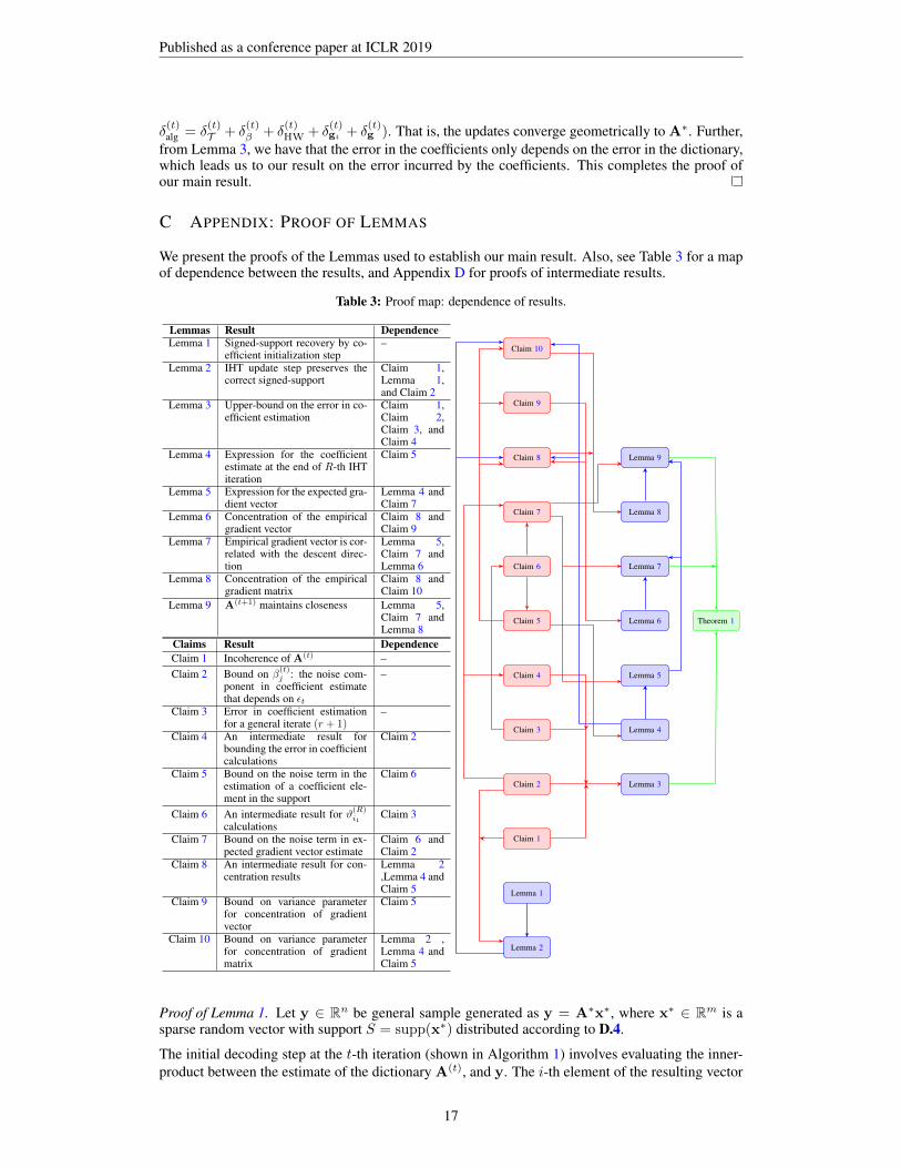
We present the proofs of the Lemmas used to establish our main result. Also, see Table 3 for a mapof dependence between the results, and Appendix D for proofs of intermediate results.

Table 3: Proof map: dependence of results.

Lemmas Result DependenceLemma 1 Signed-support recovery by co-

efficient initialization step–

Lemma 2 IHT update step preserves thecorrect signed-support

Claim 1,Lemma 1,and Claim 2

Lemma 3 Upper-bound on the error in co-efficient estimation

Claim 1,Claim 2,Claim 3, andClaim 4

Lemma 4 Expression for the coefficientestimate at the end of R-th IHTiteration

Claim 5

Lemma 5 Expression for the expected gra-dient vector

Lemma 4 andClaim 7

Lemma 6 Concentration of the empiricalgradient vector

Claim 8 andClaim 9

Lemma 7 Empirical gradient vector is cor-related with the descent direc-tion

Lemma 5,Claim 7 andLemma 6

Lemma 8 Concentration of the empiricalgradient matrix

Claim 8 andClaim 10

Lemma 9 A(t+1) maintains closeness Lemma 5,Claim 7 andLemma 8

Claims Result DependenceClaim 1 Incoherence of A(t) –Claim 2 Bound on β(t)

j : the noise com-ponent in coefficient estimatethat depends on εt

–

Claim 3 Error in coefficient estimationfor a general iterate (r + 1)

–

Claim 4 An intermediate result forbounding the error in coefficientcalculations

Claim 2

Claim 5 Bound on the noise term in theestimation of a coefficient ele-ment in the support

Claim 6

Claim 6 An intermediate result for ϑ(R)i1

calculationsClaim 3

Claim 7 Bound on the noise term in ex-pected gradient vector estimate

Claim 6 andClaim 2

Claim 8 An intermediate result for con-centration results

Lemma 2,Lemma 4 andClaim 5

Claim 9 Bound on variance parameterfor concentration of gradientvector

Claim 5

Claim 10 Bound on variance parameterfor concentration of gradientmatrix

Lemma 2 ,Lemma 4 andClaim 5

Lemma 1

Claim 1

Claim 2

Lemma 2

Claim 3

Claim 4

Lemma 3

Claim 5

Lemma 4

Lemma 5

Claim 6

Claim 7

Lemma 6

Claim 8

Claim 9

Lemma 7

Lemma 8

Claim 10

Lemma 9

Theorem 1

Proof of Lemma 1. Let y ∈ Rn be general sample generated as y = A∗x∗, where x∗ ∈ Rm is asparse random vector with support S = supp(x∗) distributed according to D.4.

The initial decoding step at the t-th iteration (shown in Algorithm 1) involves evaluating the inner-product between the estimate of the dictionary A(t), and y. The i-th element of the resulting vector

17


can be written as

〈A(t)i ,y〉 = 〈A(t)

i ,A∗i 〉x∗i + wi,

where wi = 〈A(t)i ,A∗−ix

∗−i〉. Now, since ‖A∗i −A

(t)i ‖2 ≤ εt and

‖A∗i −A(t)i ‖

22 = ‖A∗i ‖2 + ‖A(t)

i ‖2 − 2〈A(t)

i ,A∗i 〉 = 2− 2〈A(t)i ,A∗i 〉,

we have

|〈A(t)i ,A∗i 〉| ≥ 1− ε2t/2.

Therefore, the term

|〈A(t)i ,A∗i 〉x∗i |

≥ (1− ε2t

2 )C , if i ∈ S,= 0 , otherwise.

Now, we focus on the wi and show that it is small. By the definition of wi we have

wi = 〈A(t)i ,A∗−ix

∗−i〉 =

∑6=i〈A(t)

i ,A∗` 〉x∗` =∑

`∈S\i〈A(t)

i ,A∗` 〉x∗` .

Here, since var(x∗` ) = 1, wi is a zero-mean random variable with variance

var(wi) =∑

`∈S\i〈A(t)

i ,A∗` 〉2.

Now, each term in this sum can be bounded as,

〈A(t)i ,A∗` 〉2 = (〈A(t)

i −A∗i ,A∗` 〉+ 〈A∗i ,A∗` 〉)2

≤ 2(〈A(t)i −A∗i ,A

∗` 〉2 + 〈A∗i ,A∗` 〉2)

≤ 2(〈A(t)i −A∗i ,A

∗` 〉2 + µ2

n ).

Next,∑6=i〈A(t)

i −A∗i ,A∗` 〉2 can be upper-bounded as

∑`∈S\i

〈A(t)i −A∗i ,A

∗` 〉2 ≤ ‖A∗S\i‖

2ε2t .

Therefore, we have the following as per our assumptions on µ and k,

‖A∗S\i‖2 ≤ (1 + k µ√

n) ≤ 2,

using Gershgorin Circle Theorem (Gershgorin, 1931). Therefore, we have∑`∈S\i

〈A(t)i −A∗i ,A

∗` 〉2 ≤ 2ε2t .

Finally, we have that ∑`∈S\i

〈A(t)i ,A∗` 〉2 ≤ 2(2ε2t + k µ

2

n ) = O∗(ε2t ).

Now, we apply the Chernoff bound for sub-Gaussian random variables wi (shown in Lemma 12) toconclude that

Pr[|wi| ≥ C/4] ≤ 2 exp(− C2

O∗(ε2t )).

Further, wi corresponding to each m should follow this bound, applying union bound we concludethat

Pr[maxi|wi| ≥ C/4] ≤ 2m exp(− C2

O∗(ε2t )) := δ

(t)T .

18


Proof of Lemma 2. Consider the (r + 1)-th iterate x(r+1) for the t-th dictionary iterate, where‖A(t)

i − A∗i ‖ ≤ εt for all i ∈ [1,m] evaluated as the following by the update step described inAlgorithm 1,

x(r+1) = x(r) − η(r+1)x A(t)>(A(t)x(r) − y)

= (I− η(r+1)x A(t)>A(t))x(r) − η(r+1)

x A(t)>A∗x∗, (7)

where η(1)x < 1 is the learning rate or the step-size parameter. Now, using Lemma 1 we know that

x(0) (3) has the correct signed-support with probability at least (1 − δ(t)T ). Further, since A(t)>A∗

can be written as

A(t)>A∗ = (A(t) −A∗)>A∗ + A∗>A∗,

we can write the (r + 1)-th iterate of the coefficient update step using (7) as

x(r+1) = (I− η(r+1)x A(t)>A(t))x(r) − η(r+1)

x (A(t) −A∗)>A∗x∗ + η(r+1)x A∗>A∗x∗.

Further, the j-th entry of this vector is given by

x(r+1)j =(I− η(r+1)

x A(t)>A(t))(j,:)x(r) − η(r+1)

x ((A(t) −A∗)>A∗)(j,:)x∗+η(r+1)

x (A∗>A∗)(j,:)x∗.

(8)

We now develop an expression for the j-th element of each of the term in (8) as follows. First, wecan write the first term as

(I− η(r+1)x A(t)>A(t))(j,:)x

(r) = (1− η(r+1)x )x

(r)j − η

(r+1)x

∑i 6=j〈A(t)

j ,A(t)i 〉x

(r)i .

Next, the second term in (8) can be expressed as

η(r+1)x ((A(t) −A∗)>A∗)(j,:)x

∗ = η(r+1)x

∑i

〈A(t)j −A∗j ,A

∗i 〉x∗i

= η(r+1)x 〈A(t)

j −A∗j ,A∗j 〉x∗j + η(r+1)

x

∑i 6=j〈A(t)

j −A∗j ,A∗i 〉x∗i .

Finally, we have the following expression for the third term,

η(r+1)x (A∗>A∗)(j,:)x

∗ = η(r+1)x x∗j + η(r+1)

x

∑i 6=j〈A∗j ,A∗i 〉x∗i .

Now using our definition of λ(t)j = |〈A(t)

j −A∗j ,A∗j 〉| ≤

ε2t2 , combining all the results for (8), and

using the fact that since A(t) is close to A∗, vectors A(t)j −A∗j and A∗j enclose an obtuse angle, we

have the following for the j-th entry of the (r + 1)-th iterate, x(r+1) is given by

x(r+1)j = (1− η(r+1)

x )x(r)j + η(r+1)

x (1− λ(t)j )x∗j + η(r+1)

x ξ(r+1)j . (9)

Here ξ(r+1)j is defined as

ξ(r+1)j :=

∑i 6=j

(〈A(t)j −A∗j ,A

∗i 〉+ 〈A∗j ,A∗i 〉)x∗i −

∑i 6=j〈A(t)

j ,A(t)i 〉x

(r)i .

Since, 〈A∗j ,A∗i 〉 − 〈A(t)j ,A

(t)i 〉 = 〈A∗j ,A∗i −A

(t)i 〉+ 〈A∗j −A

(t)j ,A

(t)i 〉, we can write ξ(r+1)

j as

ξ(r+1)j = β

(t)j +

∑i6=j〈A(t)

j ,A(t)i 〉(x∗i − x

(r)i ), (10)

where β(t)j is defined as

β(t)j :=

∑i6=j

(〈A∗j ,A∗i −A(t)i 〉+ 〈A∗j −A

(t)j ,A

(t)i 〉+ 〈A(t)

j −A∗j ,A∗i 〉)x∗i . (11)

19


Note that β(t)j does not change for each iteration r of the coefficient update step. Further, by Claim 2

we show that |β(t)j | ≤ tβ = O(

√kεt) with probability at least (1− δ(t)

β ). Next, we define ξ(r+1)j as

ξ(r+1)j := β

(t)j +

∑i 6=j|〈A(t)

j ,A(t)i 〉||x∗i − x

(r)i |. (12)

where ξ(r+1)j ≤ ξ(r+1)

j . Further, using Claim 1,

ξ(r+1)j ≤ tβ + µt√

n‖x∗j − x

(r)j ‖1 := ξ(r+1)

max = O( k√n

), (13)

since ‖x(r−1)−x∗‖1 = O(k). Therefore, for the (r+ 1)-th iteration, we choose the threshold to be

τ (r+1) := η(r+1)x ξ(r+1)

max , (14)

and the step-size by setting the “noise” component of (9) to be smaller than the “signal” part, specif-ically, half the signal component, i.e.,

η(r+1)x ξ(r+1)

max ≤ (1−η(r+1)x )2 x

(r)min +

η(r+1)x

2 (1− ε2t2 )C,

Also, since we choose the threshold as τ (r) := η(r)x ξ

(r)max, x(r)

min = η(r)x ξ

(r)max, where x

(0)min = C/2, we

have the following for the (r + 1)-th iteration,

η(r+1)x ξ(r+1)

max ≤ (1−η(r+1)x )2 η(r)

x ξ(r)max +

η(r+1)x

2 (1− ε2t2 )C.

Therefore, for this step we choose η(r+1)x as

η(r+1)x ≤

η(r)x

2 ξ(r)max

ξ(r+1)max +

η(r)x

2 ξ(r)max−

12 (1−

ε2t2 )C

, (15)

Therefore, η(r+1)x can be chosen as

η(r+1)x ≤ c(r+1)(εt, µ, k, n),

for a small constant c(r+1)(εt, µ, k, n), η(r+1)x . In addition, if we set all η(r)

x = ηx, we have that ηx =

Ω( k√n

) and therefore τ (r) = τ = Ω(k2

n ). Further, since we initialize with the hard-thresholding step,

the entries in |x(0)| ≥ C/2. Here, we define ξ(0)max = C and η(0)

x = 1/2, and set the threshold forinitial step as η(0)

x ξ(0)max.

Proof of Lemma 3. Using the definition of ξ(`)i1

as in (12), we have

ξ(`)i1

= β(t)i1

+∑i2 6=i1

|〈A(t)i1,A

(t)i2〉||x∗i2 − x

(`−1)i2

|.

From Claim 2 we have that |β(t)i1| ≤ tβ with probability at least (1− δ(t)

β ). Further, using Claim 1 ,

and letting C(`)i := |x∗i − x

(`)i | = |x

(`)i − x∗i |, ξ

(`)i1

can be upper-bounded as

ξ(`)i1≤ β(t)

i1+ µt√

n

∑i2 6=i1

C(`−1)i2

. (16)

Rearranging the expression for (r + 1)-th update (9), and using (16) we have the following upper-bound

C(r+1)i1

≤ (1− η(r+1)x )C

(r)i1

+ η(r+1)x λ

(t)i1|x∗i1 |+ η(r+1)

x ξ(r+1)i1

.

Next, recursively substituting in for C(r)i1

, where we define∏`q=`(1− η

(q+1)x ) = 1,

C(r+1)i1

≤ C(0)i1

r∏q=0

(1− η(q+1)x ) + λ

(t)i1|x∗i1 |

r+1∑=1

η(`)x

r+1∏q=`

(1− η(q+1)x ) +

r+1∑=1

η(`)x ξ

(`)i1

r+1∏q=`

(1− η(q+1)x ).

20


Substituting for the upper-bound of ξ(`)i1

from (16),

C(r+1)i1

≤ α(r+1)i1

+ µt√n

r+1∑=1

η(`)x

∑i2 6=i1

C(`−1)i2

r+1∏q=`

(1− η(q+1)x ). (17)

Here, α(r+1)i1

is defined as

α(r+1)i1

= C(0)i1

r∏q=0

(1− η(q+1)x ) + (λ

(t)i1|x∗i1 |+ β

(t)i1

)r+1∑=1

η(`)x

r+1∏q=`

(1− η(q+1)x ). (18)

Our aim now will be to express C(`)i1

for ` > 0 in terms of C(0)i2

. Let each α(`)j ≤ α

(`)i where

j = i1, i2, . . . , ik. Similarly, let C(0)j ≤ C

(0)i for j = i1, i2, . . . , ik, and all η(`)

x = ηx. Then, using

Claim 3 we have the following expression for C(R+1)i1

,

C(R+1)i1

≤ α(R+1)i1

+ (k − 1)ηxµt√n

R∑=1

α(`)max

(1− ηx+ηx

µt√n

)R−`+ (k − 1)ηx

µt√nC(0)

max

(1− ηx + ηx

µt√n

)R.

Here, (1 − ηx)R ≤ (1 − ηx + ηxµt√n

)R ≤ δR. Next from Claim 4 we have that with probability at

least (1− δ(t)β ),

R∑=1

α(`)max

(1− ηx + ηx

µt√n

)R−` ≤ C(0)maxRδR + 1

ηx(1− µt√n

)(ε2t2 |x∗max|+ tβ).

Therefore, for cx = µt√n/(1− µt√

n)

C(R+1)i1

≤ α(R+1)i1

+ (k − 1)cx(ε2t2 |x∗max|+ tβ) + (R+ 1)(k − 1)ηx

µt√nC(0)

maxδR.

Now, using the definition of α(R+1)i1

, and using the result on sum of geometric series, we have

α(R+1)i1

= C(0)i1

(1− ηx)R+1 + (λ(t)i1|x∗i1 |+ β

(t)i1

)R+1∑s=1

ηx(1− ηx)R−s+1,

= C(0)i1δR + λ

(t)i1|x∗i1 |+ β

(t)i1≤ C(0)

i1δR+1 +

ε2t2 |x∗max|+ tβ .

Therefore, C(R)i1

is upper-bounded as

C(R)i1≤ (cxk + 1)(

ε2t2 |x∗max|+ tβ) + (R+ 1)kηx

µt√nC(0)

maxδR + C(0)i1δR.

Further, since k = O(√n/µ log(n)), kcx < 1, therefore, we have

C(R)i1≤ O(tβ) + (R+ 1)kηx

µt√nC(0)

maxδR + C(0)i1δR,

with probability at least (1−δ(t)β ). Here, (R+ 1)kηx

µt√nC

(0)maxδR+C

(0)i1δR u 0 for an appropriately

large R. Therefore, the error in each non-zero coefficient is

C(R)i1

= O(tβ).

with probability at least (1− δ(t)β ).

Proof of Lemma 4. Using the expression for x(R)i1

as defined in (9), and recursively substituting for

x(r)i1

we have

x(R)i1

= (1− ηx)Rx(0)j + x∗i1

R∑r=1

ηx(1− λ(t)i1

)(1− ηx)R−r +R∑r=1

ηxξ(r)i1

(1− ηx)R−r,

21


where we set all ηrx to be ηx. Further, on defining

ϑ(R)i1

:=R∑r=1

ηxξ(r)i1

(1− ηx)R−r + γ(R)i1

, (19)

where γ(R)i1

:= (1− ηx)R(x(0)i1− x∗i1(1− λ(t)

i1)), we have

x(R)i1

= (1− ηx)Rx(0)i1

+ x∗i1(1− λ(t)i1

)(1− (1− ηx)R) +R∑r=1

ηxξ(r)i1

(1− ηx)R−r,

= x∗i1(1− λ(t)i1

) + ϑ(R)i1. (20)

Note that γ(R)i1

can be made appropriately small by choice of R. Further, by Claim 5 we have

|ϑ(R)i1| ≤ O(tβ).

with probability at least (1− δ(t)β ), where tβ = O(

√kεt).

Proof of Lemma 5. From Lemma 4 we have that for each j ∈ S,

xS := x(R)S = (I− Λ

(t)S )x∗S + ϑ

(R)S ,

with probability at least (1 − δ(t)T − δ

(t)β ). Further, let Fx∗ be the event that sign(x∗) = sign(x),

and let 1Fx∗ denote the indicator function corresponding to this event. As we show in Lemma 2,this event occurs with probability at least (1 − δ(t)

β − δ(t)T ). Using this, we can write the expected

gradient vector corresponding to the j-th sample as 1Fx∗

g(t)j = E[(A(t)x− y)sign(x∗j )1Fx∗ ] + E[(A(t)x− y)sign(x∗j )1Fx∗

],

= E[(A(t)x− y)sign(x∗j )1Fx∗ ]± γ.

Here, γ := E[(A(t)x − y)sign(x∗j )1Fx∗] is small and depends on δ

(t)T and δ

(t)β , which in turn

drops with εt. Therefore, γ diminishes with εt. Further, since 1Fx∗ + 1Fx∗= 1, and Pr[Fx∗ ] =

(1− δ(t)β − δ

(t)T ), is very large,

g(t)j = E[(A(t)x− y)sign(x∗j )(1− 1Fx∗

)]± γ,

= E[(A(t)x− y)sign(x∗j )]± γ.

Therefore, we can write g(t)j as

g(t)j = E[(A(t)x− y)sign(x∗j )]± γ,

= E[(1− ηx)RA(t)S x

(0)S + A

(t)S (I− Λ

(t)S )x∗S + A

(t)S ϑ

(R)S −A∗Sx

∗S)sign(x∗j )]± γ.

Since E[(1 − ηx)RA(t)S x

(0)S ] can be made very small by choice of R, we absorb this term in γ.

Therefore,

g(t)j = E[A

(t)S (I− Λ

(t)S )x∗S + A

(t)S ϑ

(R)S −A∗Sx

∗S)sign(x∗j )]± γ.

Writing the expectation by sub-conditioning on the support,

g(t)j = ES [Ex∗S [A

(t)S (I− Λ

(t)S )x∗Ssign(x∗j )−A∗Sx

∗Ssign(x∗j ) + A

(t)S ϑ

(R)S sign(x∗j )|S]]± γ,

= ES [A(t)S (I− Λ

(t)S )Ex∗S [x∗Ssign(x∗j )|S]−A∗SEx∗S [x∗Ssign(x∗j )|S]] + E[A

(t)S ϑ

(R)S sign(x∗j )]± γ,

= ES [pj(1− λ(t)j )A

(t)j − pjA

∗j ] + ∆

(t)j ± γ,

where we have used the fact that Ex∗S [sign(x∗j )] = 0 and introduced

∆(t)j = E[A

(t)S ϑ

(R)S sign(x∗j )].

22


Next, since pj = Ex∗S [x∗j sign(x∗j )|j ∈ S], therefore,

g(t)j = ES [pj(1− λ(t)

j )A(t)j − pjA

∗j ] + ∆

(t)j ± γ.

Further, since qj = Pr[j ∈ S] = O(k/m),

g(t)j = qjpj

((1− λ(t)

j )A(t)j −A∗j + 1

qjpj∆

(t)j ± γ

).

Further, by Claim 7 we have that

‖∆(t)j ‖ = O(

√mqi,jpjεt‖A(t)‖)].

This completes the proof.

Proof of Lemma 6. Let W = j : i ∈ supp(x∗(j)) and then we have that

g(t)i = |W |

p1|W |∑j(y(j) −A(t)x(j))sign(x(j)(i)),

where x(j)(i) denotes the i-th element of the coefficient estimate corresponding to the (j)-th sample.Here, for ` = |W | the summation∑

j1` (y(j) −A(t)x(j))sign(x(j)(i)),

has the same distribution as Σ`j=1zj , where each zj belongs to a distribution as

z := 1` (y −A(t)x)sign(xi)|i ∈ S.

Also, E[(y − A(t)x)sign(xi)] = qiE[z], where qi = Pr[x∗i 6= 0] = Θ( km ). Therefore, sincep = Ω(mk2), we have ` = pqi = Ω(k3) non-zero vectors,

‖g(t)i − g

(t)i ‖ = O( km )‖Σ`j=1(zj −E[z])‖. (21)

Let wj = zj − E[z], we will now apply the vector Bernstein result shown in Lemma 11. For this,we require bounds on two parameters for these – L := ‖wj‖ and σ2 := ‖ΣjE[‖wj‖2]‖. Note that,since the quantity of interest is a function of x∗i , which are sub-Gaussian, they are only boundedalmost surely. To this end, we will employ Lemma 14 (Lemma 45 in (Arora et al., 2015)) to get ahandle on the concentration.

Bound on the norm ‖w‖: This bound is evaluated in Claim 8, which states that with probabilityat least (1− δ(t)

β − δ(t)T − δ

(t)HW),

L := ‖w‖ = ‖z−E[z]‖ = 2` ‖(y −A(t)x)sign(xi)|i ∈ S‖ ≤ 2

` ‖(y −A(t)x)‖ = O(ktβ` ).

Bound on variance parameter E[‖w‖2]: Using Claim 9, we have E[‖z‖2] = O(kε2t ) + O(kt2β).Therefore, the bound on the variance parameter σ2 is given by

σ2 := ‖ΣjE[‖wj‖2]‖ ≤ ‖ΣjE[‖zj‖2]‖ ≤ O(k` ε2t ) +O(

kt2β` ).

From Claim 2 we have that with probability at least (1 − δ(t)β ), tβ = O(

√kεt). Applying vector

Bernstein inequality shown in Lemma 11 and using Lemma 14 (Lemma 45 in (Arora et al., 2015)),choosing ` = Ω(k3), we conclude

‖∑`j=1 zj −E[z]‖ = O(L) +O(σ) = o(εt),

with probability at least (1− δ(t)gi ), where δ(t)

gi = exp(−Ω(k)). Finally, substituting in (21) we have

‖g(t)i − g

(t)i ‖ = O( km )o(εt).

with probability at least (1− δ(t)gi − δ

(t)β − δ

(t)T − δ

(t)HW).

23


Proof of Lemma 7. Since we only have access to the empirical estimate of the gradient g(t)i , we will

show that this estimate is correlated with (A(t)j −A∗j ). To this end, first from Lemma 6 we have that

the empirical gradient vector concentrates around its mean, specifically,

‖g(t)i − g

(t)i ‖ ≤ o( kmεt),

with probability at least (1 − δ(t)gi − δ

(t)β − δ

(t)T − δ

(t)HW). From Lemma 5, we have the following

expression for the expected gradient vector

g(t)j = pjqj(A

(t)j −A∗j ) + pjqj(−λ(t)

j A(t)j + 1

pjqj∆

(t)j ± γ).

Let g(t)j = 4ρ (A

(t)j −A∗j ) + v, where 4ρ = pjqj and v is defined as

v = pjqj(−λ(t)j A

(t)j + 1

pjqj∆

(t)j ± γ). (22)

Then, g(t)i can be written as

g(t)i = g

(t)i − g

(t)i + g

(t)i ,

= (g(t)i − g

(t)i ) + 4ρ (A

(t)j −A∗j ) + v,

= 4ρ (A(t)j −A∗j ) + v, (23)

where v = v + (g(t)i − g

(t)i ). Let ‖v‖ ≤ ρ ‖A(t)

i −A∗i ‖. Using the definition of v as shown in (22)we have

‖v‖ ≤ qjpjλ(t)j ‖A

(t)j ‖+ ‖∆(t)

j ‖+ o( kmεt)± γ.

Now for the first term, since ‖A(t)j ‖ = 1, we have λ(t)

j = |〈A(t)j −A∗j ,A

∗j 〉| = 1

2‖A(t)j −A∗j‖2,

therefore

qjpjλ(t)j ‖A

(t)j ‖ = qjpj

12‖A

(t)j −A∗j‖2,

Further, using Claim 7

‖∆(t)j ‖ = O(

√mqi,jpi1εt‖A(t)‖).

Now, since ‖A(t)−A∗‖ ≤ 2‖A∗‖ (the closeness property (Def.1) is maintained at every step usingLemma 9), and further since ‖A∗‖ = O(

√m/n), we have that

‖A(t)‖ ≤ ‖A(t) −A∗‖+ ‖A∗‖ = O(√

mn ).

Therefore, we have

‖∆(t)j ‖+ o( kmεt)± γ = O(

√mqi,jpi1εt‖A(t)‖).

Here, we use the fact that γ drops with decreasing εt as argued in Lemma 5. Next, using (23), wehave

‖g(t)j ‖ ≤ 4ρ ‖A(t)

j −A∗j‖+ ‖v‖.

Now, letting

‖∆(t)j ‖+ o( kmεt)± γ = O(

√mqi,jpi1εt‖A(t)‖) ≤ qipi

2 ‖A(t)j −A∗j‖, (24)

we have that, for k = O(√n)

‖v‖ ≤ qipi‖A(t)j −A∗j‖.

Substituting for ‖v‖, this implies that ‖g(t)j‖2 ≤ 25ρ2‖A(t)

j − A∗j‖2. Further, we also have thefollowing lower-bound

〈g(t)j ,A

(t)j −A∗j 〉 ≥ 4ρ ‖A(t)

j −A∗j‖2 − ‖v‖‖A(t)j −A∗j‖.

24


Here, we use the fact that R.H.S. can be minimized only if v is directed opposite to the direction ofA

(t)j −A∗j . Now, we show that this gradient is (ρ , 1/100ρ , 0) correlated,

〈g(t)i ,A

(t)i −A

∗i 〉 − ρ ‖A

(t)i −A∗i ‖2 − 1

100ρ ‖g(t)i ‖

2,

≥ 4ρ ‖A(t)i −A∗i ‖2 − ‖v‖‖A

(t)i −A∗i ‖ − ρ ‖A

(t)i −A∗i ‖2 − 1

100ρ ‖g(t)i ‖

2,

≥ 4ρ ‖A(t)i −A∗i ‖2 − 2ρ ‖A(t)

i −A∗i ‖2 −25ρ2‖A(t)

i −A∗i ‖

2

100ρ ,

≥ ρ ‖A(t)i −A∗i ‖2 ≥ 0.

Therefore, for this choice of k, i.e. k = O(√n), there is no bias in dictionary estimation in compar-

ison to Arora et al. (2015). This gain can be attributed to estimating the coefficients simultaneouslywith the dictionary. Further, since we choose 4ρ = pjqj , we have that ρ = Θ(k/m), as a resultρ

+= 1/100ρ = Ω(m/k). Applying Lemma 15 we have

‖A(t+1)j −A∗j‖2 ≤ (1− ρ ηA)‖A(t)

j −A∗j‖2,

for ηA = O(m/k) with probability at least (1− δ(t)T − δ

(t)β − δ

(t)gi ).

Proof of Lemma 8. Here, we will prove that g(t) defined as

g(t) =∑j(y(j) −A(t)x(j))sign(x(j))

>,

concentrates around its mean. Notice that each summand (y(j)−A(t)x(j))sign(x(j))> is a random

matrix of the form (y −A(t)x)sign(x)>. Also, we have g(t) defined as

g(t) = E[(y −A(t)x)sign(x)>].

To bound ‖g(t) − g(t)‖, we are interested in ‖∑pj=1 Wj‖, where each matrix Wj is given by

Wj = 1p (y(j) −A(t)x(j))sign(x(j))

> − 1pE[(y −A(t)x)sign(x)>].

Noting that E[Wj ] = 0, we will employ the matrix Bernstein result (Lemma 10) to bound ‖g(t) −g(t)‖. To this end, we will bound ‖Wj‖ and the variance proxy

v(Wj) = max‖∑pj=1 E[WjW

>j ]‖, ‖

∑pj=1 E[W>

j Wj ]‖.

Bound on ‖Wj‖– First, we can bound both terms in the expression for Wj by triangle inequalityas

‖Wj‖ ≤ 1p‖(y(j) −A(t)x(j))sign(x(j))

>‖+ 1p‖E[(y −A(t)x)sign(x)>‖,

≤ 2p‖(y −A(t)x)sign(x)>‖.

Here, we use Jensen’s inequality for the second term, followed by upper-bounding the expectedvalue of the argument by ‖(y −A(t)x)sign(x)>‖.

Next, using Claim 8 we have that with probability at least (1− δ(t)β − δ

(t)T − δ

(t)HW), ‖y −A(t)x‖ is

O(ktβ), and the fact that ‖sign(x)T ‖ =√k,

‖Wj‖ ≤ 2p

√k‖(y −A(t)x)‖ = O(k

√k

p tβ).

Bound on the variance statistic v(Wj)– For the variance statistic, we first look at‖∑

E[WjW>j ]‖,

E[WjW>j ] = 1

p2E[(y(j) −A(t)x(j))sign(x(j))> −E[(y −A(t)x)sign(x)>]

× [sign(x(j))(y(j) −A(t)x(j))> − (E[(y −A(t)x)sign(x)>)>].

Since E[(y −A(t)x)sign(x)>]E[(y −A(t)x)sign(x)>]> is positive semidefinite,

E[WjW>j ] 1

p2E[(y(j) −A(t)x(j))sign(x(j))>sign(x(j))(y(j) −A(t)x(j))

>].

25


Now, since each x(j) has k non-zeros, sign(x(j))>sign(x(j)) = k, and using Claim 10, with proba-

bility at least (1− δ(t)T − δ

(t)β )

‖∑

E[WjW>j ]‖ ≤ k

p‖E[(y(j) −A(t)x(j))(y(j) −A(t)x(j))>]‖,

= O(k3t2βpm )‖A∗‖2.

Similarly, expanding E[W>j Wj ], and using the fact that E[(y − A(t)x)sign(x)>]>E[(y −

A(t)x)sign(x)>] is positive semi-definite. Now, using Claim 8 and the fact that entries ofE[(sign(x(j))sign(x(j))

>] are qi on the diagonal and zero elsewhere, where qi = O(k/m),

‖∑

E[W>j Wj ]‖ 1

p‖E[(sign(x(j))(y(j) −A(t)x(j))>(y(j) −A(t)x(j))sign(x

(R)(j) )>]‖,

≤ 1p‖E[(sign(x(j))sign(x(j))

>]‖‖y(j) −A(t)x(j)‖2,

≤ O( kmp )O(k2t2β) = O(

k3t2βmp ).

Now, we are ready to apply the matrix Bernstein result. Since, m = O(n) the variance statistic

comes out to be O(k3t2βpm )‖A∗‖2, then as long as we choose p = Ω(mk2) (using the bound on tβ),

with probability at least (1− δ(t)β − δ

(t)T − δ

(t)HW − δ

(t)g )

‖g(t) − g(t)‖ ≤ O(k√k

p tβ) + ‖A∗‖√O(

k3t2βpm ),

= O∗( km‖A∗‖).

where δ(t)g = (n+m) exp(−Ω(m

√log(n)).

Proof of Lemma 9. This lemma ensures that the dictionary iterates maintain the closeness property(Def.1) and satisfies the prerequisites for Lemma 7.

The update step for the i-th dictionary element at the s+ 1 iteration can be written as

A(t+1)i −A∗i = A

(t)i −A∗i − ηAg

(t)i ,

= A(t)i −A∗i − ηAg

(t)i − ηA(g

(t)i − g

(t)i ).

Here, g(t)i is given by the following as per Lemma 5 with probability at least (1− δ(t)

T − δ(t)β )

g(t)i = qipi(A

(t)i −A∗i ) + qipi(−λ(t)

i A(t)i + 1

qipi∆

(t)i ± γ).

Substituting the expression for g(t)i in the dictionary update step,

A(t+1)i −A∗i = (1− ηApiqi)(A(t)

i −A∗i )− ηApiqiλ(t)i A

(t)i − ηA∆

(t)i − ηA(g

(t)i − g

(t)i )± γ,

where ∆(t)j = E[A(t)ϑ(R)sign(x∗j )]j . Therefore, the update step for the dictionary (matrix) can be

written as

A(t+1) −A∗ = (A(t) −A∗)diag((1− ηApiqi)) + ηAU− ηAV ± γ − ηA(g(t) − g(t)), (25)

where, U = A(t)diag(piqiλ(t)i ) and V = A(t)Q, with the matrix Q given by,

Qi,j = qi,jEx∗S[ϑ

(R)i sign(x∗j )|S],

and using the following intermediate result shown in Claim 7,

Ex∗S[ϑ

(R)i sign(x∗j )|S]

≤ γ(R)

i , for i = j,

= O(pjεt), for i 6= j,

we have ‖Qi‖ = O(√mqi,jpiεt). Hence, we have

‖Q‖F ≤ O(mqi,jpiεt).

26


Therefore,

‖V‖ ≤ ‖A(t)Q‖ ≤ ‖A(t)‖‖Q‖F = O(mqi,jpiεt‖A∗‖) = O( k2

m log(n) )‖A∗‖.

We will now proceed to bound each term in (25). Starting with (A(t) −A∗)diag(1− ηApiqi), andusing the fact that pi = O(1), qi = O(k/m), and ‖A(t) −A∗‖ ≤ 2‖A∗‖, we have

‖(A(t) −A∗)diag(1− ηApiqi)‖ ≤ (1−miniηApiqi)‖(A(t) −A∗)‖ ≤ 2(1− Ω(ηAk/m))‖A∗‖.

Next, since ‖A(t)j ‖ = 1, we have λ(t)

j = |〈A(t)j −A∗j ,A

∗j 〉| = 1

2‖A(t)j −A∗j‖2, and λ(t)

i ≤ ε2t/2,therefore

‖U‖ = ‖A(t)diag(piqiλ(t)i )‖ ≤ max

ipiqi

ε2t2 ‖A

(t) −A∗ + A∗‖ ≤ o(k/m)‖A∗‖.

Using the results derived above, and the the result derived in Lemma 8 which states that with prob-ability at least (1− δ(t)

β − δ(t)T − δ

(t)HW − δ

(t)g ), ‖g(t) − g(t)‖ = O∗( km‖A

∗‖)) we have

‖A(t+1)−A∗‖ = ‖(A(t) −A∗)D(1−ηApiqi)‖+ ηA‖U‖+ ηA‖V‖+ ηA‖(g(t) − g(t))‖ ± γ,

≤ 2(1− Ω(ηAkm )‖A∗‖+ o(ηA

km )‖A∗‖+O(ηA

k2

m log(n) )‖A∗‖+ o(ηAkm‖A

∗‖)± γ,≤ 2‖A∗‖.

27


D APPENDIX: PROOFS OF INTERMEDIATE RESULTS

Claim 1 (Incoherence of A(t)). If A∗ ∈ Rn×m is µ-incoherent and ‖A∗i −A(t)i ‖ ≤ εt holds for

each i ∈ [1 . . .m], then A(t) ∈ Rn×m is µt-incoherent, where µt = µ+ 2√nεt.

Proof of Claim 1. We start by looking at the incoherence between the columns of A∗, for j 6= i,

〈A∗i ,A∗j 〉 = 〈A∗i −A(t)i ,A∗j 〉+ 〈A(t)

i ,A∗j 〉,

= 〈A∗i −A(t)i ,A∗j 〉+ 〈A(t)

i ,A∗j −A(t)j 〉+ 〈A(t)

i ,A(t)j 〉.

Since 〈A∗i ,A∗j 〉 ≤µ√n

,

|〈A(t)i ,A

(t)j 〉| ≤ 〈A

∗i ,A

∗j 〉 − 〈A∗i −A

(t)i ,A∗j 〉 − 〈A

(t)i ,A∗j −A

(t)j 〉,

≤ µ√n

+ 2εt.

Claim 2 (Bound on β(t)j : the noise component in coefficient estimate that depends on εt). With

probability (1− δ(t)β ), |β(t)

j | is upper-bounded by tβ = O(√kεt), where δ(t)


).

Proof of Claim 2. We have the following definition for β(t)j from (11),

β(t)j =

∑i 6=j

(〈A∗j ,A∗i −A(t)i 〉+ 〈A∗j −A

(t)j ,A

(t)i 〉+ 〈A(t)

j −A∗j ,A∗i 〉)x∗i .

Here, since x∗i are independent sub-Gaussian random variables, β(t)j is a sub-Gaussian random vari-

able with the variance parameter evaluated as shown below

var[β(t)j ] =

∑i 6=j(〈A∗j ,A

(t)i −A∗i 〉+ 〈A(t)

j −A∗j ,A(t)i 〉+ 〈A(t)

j −A∗j ,A∗i 〉)2 ≤ 9kε2t .

Therefore, by Lemma 12

Pr[|β(t)j | > tβ ] ≤ 2exp(− t2β

18kε2t).

Now, we need this for each β(t)j for j ∈ supp(x∗), union bounding over k coefficients

Pr[max |β(t)j | > tβ ] ≤ δ(t)

β ,

where δ(t)β = 2k exp(− t2β

18kε2t). Choosing tβ = O(

√kεt), we have that δ(t)


).

Claim 3 (Error in coefficient estimation for a general iterate (r + 1)). The error in a generaliterate r of the coefficient estimation is upper-bounded as

C(r+1)i1

≤ α(r+1)i1


r∑=1

α(`)max

(1− ηx + ηx

µt√n

)r−`+ (k − 1)ηx

µt√nC(0)

max

(1− ηx + ηx

µt√n

)r.

Proof of Claim 3 . From (17) we have the following expression for C(r+1)i1

C(r+1)i1

≤ α(r+1)i1

+ µt√n

r+1∑=1

η(`)x

∑i2 6=i1

C(`−1)i2

r+1∏q=`

(1− η(q+1)x ).

Our aim will be to recursively substitute for C(`−1)i1

to develop an expression for C(r+1)i1

as a func-

tion of C0max. To this end, we start by analyzing the iterates C(1)

i1, C(2)

i1, and so on to develop an

expression for C(r+1)i1

as follows.

28


Expression for C(1)i1

– Consider C(1)i1

C(1)i1≤ α(1)

i1+ µt√

n

1∑=1

ηx∑i2 6=i1

C(`−1)i2

1∏q=`

(1− ηx),

= α(1)i1

+ ηx(µt√n

∑i1 6=i2

C(0)i2

). (26)


– Next, C(2)i1

is given by

C(2)i1≤ α(2)

i1+ ηx

µt√n

2∑=1

∑i2 6=i1

C(`−1)i2

2∏q=`

(1− ηx),

≤ α(2)i1

+ ηxµt√n

( ∑i2 6=i1

C(1)i2

+∑i2 6=i1

C(0)i2

(1− ηx)).

Further, we know from (26) we have

C(1)i2

= α(1)i2

+ ηxµt√n

∑i3 6=i2

C(0)i3.

Therefore, since∑i2 6=i1

∑i3 6=i2

=∑

i3 6=i2,i1,

C(2)i1≤ α(2)

i1+ ηx

µt√n

( ∑i2 6=i1

(α

(1)i2

+ ηxµt√n

∑i3 6=i2

C(0)i3

)+∑i2 6=i1

C(0)i2

(1− ηx)),

= α(2)i1

+ ηxµt√n

∑i2 6=i1

α(1)i2

+ ηxµt√n

(ηx

µt√n

∑i3 6=i2,i1

C(0)i3

+∑i2 6=i1

C(0)i2

(1− ηx)). (27)


– Next, we writing C(3)i1

,

C(3)i1≤ α(3)

i1+ ηx

µt√n

∑3`=1

∑i2 6=i1

C(`−1)i2

(1− ηx)3−`,

= α(3)i1

+ ηxµt√n

∑i2 6=i1

(C

(0)i2

(1− ηx)2 + C(1)i2

(1− ηx) + C(2)i2

),

≤ α(3)i1

+ ηxµt√n

∑i2 6=i1

(C

(0)i2

(1− ηx)2 +(α

(1)i2

+ ηxµt√n

∑i3 6=i2

C(0)i3

)(1− ηx) + C

(2)i2

).

Here, using (27) we have the following expression for C(2)i2

C(2)i2≤ α(2)

i2+ ηx

µt√n

∑i3 6=i2

α(1)i3

+ ηxµt√n

(ηx

µt√n

∑i4 6=i3,i2

C(0)i4

+∑i3 6=i2

C(0)i3

(1− ηx)).

Substituting forC(2)i2

in the expression forC(3)i1

, and rearranging the terms in the expression forC(3)i1

,we have

C(3)i1≤ α(3)

i1+ ηx

µt√n

∑i2 6=i1

α(2)i2

+ ηxµt√n

((1− ηx)

∑i2 6=i1

α(1)i2

+ ηxµt√n

∑i3 6=i2,i1

α(1)i3

)+ ηx

µt√n

((1− ηx)2 ∑

i2 6=i1C

(0)i2

+ 2(1− ηx)(ηxµt√n

)∑

i3 6=i2,i1C

(0)i3

+ (ηxµt√n

)2∑

i4 6=i3,i2,i1C

(0)i4

).

(28)


– Now, consider C(4)i1

C(4)i1≤ α(4)

i1+ ηx

µt√n

∑4`=1

∑i2 6=i1 C

(`−1)i2

(1− ηx)4−`,

≤ α(4)i1

+ ηxµt√n

(∑i2 6=i1 C

(0)i2

(1− ηx)3 +∑i2 6=i1 C

(1)i2

(1− ηx)2 +∑i2 6=i1 C

(2)i2

(1− ηx)1

+∑i2 6=i1 C

(3)i2

(1− ηx)0).

Substituting for C(3)i2

from (28), C(2)i2

from (27), C(1)i2

using (26), and rearranging,

C(4)i1≤ α(4)

i1+ ηx

µt√n

[ ∑i2 6=i1

α(3)i2

+

((1− ηx)1

∑i2 6=i1 α

(2)i2

+ ηxµt√n

∑i3 6=i2,i1

α(2)i3

)

29


+( ∑i2 6=i1

α(1)i2

(1− ηx)2 + 2ηxµt√n

(1− ηx)∑

i3 6=i2,i1α

(1)i3

+ (ηxµt√n

)2∑

i4 6=i3,i2,i1α

(1)i4

)]+ ηx

µt√n

[ ∑i2 6=i1

C(0)i2

(1− ηx)3 + 3ηxµt√n

(1− ηx)2∑

i3 6=i2,i1C

(0)i3

+ 3(ηxµt√n

)2(1− ηx)1 ∑i4 6=i3,i2,i1

C(0)i4

+ (ηxµt√n

)3∑

i5 6=i4,i3,i2,i1C

(0)i5

].

Notice that the terms have a binomial series like form. To reveal this structure, let each α(`)j ≤ α

(`)max

where j = i1, i2, . . . , ik. Similarly, let C(0)j ≤ C(0)

max for j = i1, i2, . . . , ik. Therefore, we have

C(4)i1≤ α(4)

i1+ ηx

µt√n

[(k − 1)α

(3)i + α

(2)i

((1− ηx)1(k − 1) + ηx

µt√n

(k − 2)

)+ α

(1)i

((k − 1)(1− ηx)2 + 2(k − 2)ηx

µt√n

(1− ηx) + (k − 3)(ηxµt√n

)2

)]+ ηx

µt√nC

(0)i

[(k − 1)(1− ηx)3 + 3(k − 2)ηx

µt√n

(1− ηx)2

+ 3(k − 3)(ηxµt√n

)2(1− ηx)1 + (k − 4)(ηxµt√n

)3

].

Further upper-bounding the expression, we have

C(4)i1≤ α(4)

i1+ (k − 1)ηx

µt√n

[α

(3)i + α

(2)i

((1− ηx) + ηx

µt√n

)+ α

(1)i

((1− ηx)2 + 2ηx

µt√n

(1− ηx) + (ηxµt√n

)2

)]+ (k − 1)ηx

µt√nC

(0)i

[(1− ηx)3 + 3ηx

µt√n

(1− ηx)2 + 3(ηxµt√n

)2(1− ηx) + (ηxµt√n

)3

].

Therefore,

C(4)i1≤ α(4)

i1+ (k − 1)ηx

µt√n

[α

(3)i +α

(2)i

(1− ηx + ηx

µt√n

)1+ α

(1)i

(1− ηx + ηx

µt√n

)2]+ (k − 1)ηx

µt√nC

(0)i

(1− ηx + ηx

µt√n

)3. (29)

Expression for C(r+1)i1

– With this, we are ready to write the general term,

C(r+1)i1

≤ α(r+1)i1


r∑=1

α(`)max

(1− ηx + ηx

µt√n

)r−`+ (k − 1)ηx

µt√nC(0)

max

(1− ηx + ηx

µt√n

)r.

Claim 4 (An intermediate result for bounding the error in coefficient calculations). With prob-ability (1− δ(t)

T − δ(t)β ),

R∑=1

α(`)max

(1− ηx + ηx

µt√n

)R−` ≤ C(0)i RδR + 1

ηx(1− µt√n

)(ε2t2 |x∗max|+ tβ).

Proof of Claim 4 . Using (18), the quantity α(`)i is defined as

α(`)i = C

(0)i (1− ηx)` + (λ

(t)i |x

∗i |+ β

(t)i )

∑s=1

ηx(1− ηx)`−s+1.

30


Therefore, we are interested in

R∑=1

C(0)i (1− ηx)`

(1− ηx+ηx

µt√n

)R−`+ (λ

(t)i |x∗i |+ β

(t)i )

R∑=1

(1− ηx + ηx

µt√n

)R−` ∑s=1

ηx(1− ηx)`−s+1.

Consider the first term which depends on C(0)i . Since (1− ηx) ≤ (1− ηx + ηx

µt√n

), we have

C(0)i

R∑=1

(1− ηx)`(1− ηx + ηx

µt√n

)R−` ≤ C(0)i R

(1− ηx + ηx

µt√n

)R ≤ C(0)i RδR,

where δR is a small constant, and a parameter which determines the number of iterations R requiredfor the coefficient update step. Now, coming back to the quantity of interest

R∑=1

α(`)i

(1− ηx + ηx

µt√n

)R−` ≤ C(0)i RδR

+ (λ(t)i |x∗i |+ β

(t)i )

R∑=1

(1− ηx + ηx

µt√n

)R−` ∑s=1

ηx(1− ηx)`−s+1.

Now, using sum of geometric series result, we have that∑s=1

ηx(1− ηx)`−s+1, and

R∑=1

(1− ηx + ηx

µt√n

)R−`=

1−(

1−ηx+ηxµt√n

)Rηx−ηx

µt√n

≤ 1

ηx(1− µt√n

).

Therefore, with probability at least (1− δ(t)β ),

R∑=1

α(`)max

(1− ηx + ηx

µt√n

)R−` ≤ C(0)i RδR + 1

ηx(1− µt√n

)(ε2t2 |x∗max|+ tβ),

where λ(t)i ≤

ε2t2 and |β(t)

i | = tβ with probability at least (1− δ(t)β ) using Claim 2.

Claim 5 (Bound on the noise term in the estimation of a coefficient element in the support).With probability (1− δ(t)

β ), each entry ϑ(R)i1

of ϑ(R) is upper-bounded as

|ϑ(R)i1| ≤ O(tβ).

Proof of Claim 5. From (19) ϑ(R)i1

is defined as

ϑ(R)i1

:=R∑r=1

ηxξ(r)i1

(1− ηx)R−r + γ(R)i1

,

where γ(R)i1

:= (1− ηx)R(x(0)i1− x∗i1(1− λ(t)

i1)). Further, ξ(r)

i1is as defined in (10),

ξ(r)i1

= β(t)i1

+∑i2 6=i1

|〈A(t)i1,A

(t)i2〉|sign(〈A(t)

i1,A

(t)i2〉)C(r−1)

i2sign(x∗i2 − x

(r)i2

).

Therefore, we have the following expression for ϑ(R)i1

ϑ(R)i1

=β(t)i1

R∑r=1

ηx(1− ηx)R−r

+R∑r=1

ηx∑i2 6=i1

|〈A(t)i1,A

(t)i2〉|sign(〈A(t)

i1,A

(t)i2〉)C(r−1)

i2sign(x∗i2 − x

(r)i2

)(1− ηx)R−r + γ(R)i1

.

(30)

31


Now ϑ(R)i1

can be upper-bounded as

ϑ(R)i1≤ β(t)

i1

R∑r=1

ηx(1− ηx)R−r + ηxµt√n

R∑r=1

∑i2 6=i1 C

(r−1)i2

(1− ηx)R−r + γ(R)i1

,

≤ β(t)i1


R∑r=1

C(r−1)i2

(1− ηx)R−r + γ(R)i1

.

Since from Claim 6 we have

C(r−1)i2

(1− ηx)R−r ≤ (λ(t)max|x∗max|+ β(t)

max)[ r−1∑s=1

ηx(1− ηx)R−s + kcx(1− ηx)R−r]

+ kηxµt√nC(0)

maxδR−2.

Further, since 1− (1− ηx)r−1 ≤ 1, we have thatR∑r=1

r−1∑s=1

ηx(1− ηx)R−s =R∑r=1

ηx(1− ηx)R−r+1 1−(1−ηx)r−1

ηx≤

R∑r=1

(1− ηx)R−r+1 ≤ 1ηx.

Therefore,

|ϑ(R)i1| ≤ |β(t)

i1|+ (k − 1) µt√

n(λ(t)

max|x∗max|+ |β(t)max|)(1 + kcx) +

(kηx

µt√n

)2RC(0)

maxδR−2 + γ(R)i1

.

Now, since each |β(t)i | = tβ with probability at least (1 − δ

(t)β ) for the t-th iterate, and k =

O∗(√n

µ log(n) ), therefore kcx < 1, we have that

|ϑ(R)i1| ≤ O(tβ).

with probability at least (1− δ(t)β ).

Claim 6 (An intermediate result for ϑ(R)i1

calculations). For cx = µt√n/(1− µt√

n), we have

C(r−1)i2

(1− ηx)R−r≤ (λ(t)max|x∗max|+ β(t)

max)

[r−1∑s=1


+ kηxµt√nC(0)

maxδR−2.

Proof of Claim 6. Here, from Claim 3 we have that for any i1,

C(r+1)i1

≤ α(r+1)i1

+ kηxµt√n

r∑=1

α(`)max

(1− ηx + ηx

µt√n

)r−`+ kηx

µt√nC

(0)max

(1− ηx + ηx

µt√n

)r.

therefore C(r−1)i2

is given by

C(r−1)i2

≤ α(r−1)i2

+ kηxµt√n

r−2∑=1

α(`)max

(1− ηx + ηx

µt√n

)r−`−2+kηx

µt√nC

(0)max

(1− ηx + ηx

µt√n

)r−2.

Further, the term of interest C(r−1)i2

(1− ηx)R−r can be upper-bounded by

C(r−1)i2

(1− ηx)R−r≤ α(r−1)i2

(1− ηx)R−r+(1− ηx)R−rkηxµt√n

r−2∑=1

α(`)max

(1− ηx + ηx

µt√n

)r−`−2

+ kηxµt√nC(0)

max

(1− ηx + ηx

µt√n

)r−2(1− ηx)R−r.

From the definition of α(`)i from (18), α(r−1)

i2can be written as

α(r−1)i2

= C(0)max(1− ηx)r−1 + (λ(t)

max|x∗max|+ β(t)max)

r−1∑s=1

ηx(1− ηx)r−s.

Therefore, we have

α(r−1)i2

(1− ηx)R−r = C(0)max(1− ηx)R−1 + (λ(t)


r−1∑s=1

ηx(1− ηx)R−s.

32


Next, to get a handle on α(`)max

(1− ηx + ηx

µt√n

)r−`−2, consider the following using the definition of

α(`)i from (18), where η(i)

x = ηx for all i,

r∑=1

α(`)max

(1−ηx + ηx

µt√n

)r−`=

r∑=1

C(0)max(1− ηx)`

(1− ηx + ηx

µt√n

)r−`+ (λ(t)


r∑=1

(1− ηx + ηx

µt√n

)r−` ∑s=1

ηx(1− ηx)`−s+1,

≤r∑=1

C(0)max

(1− ηx + ηx

µt√n

)r+ (λ

(t)max|x∗max|+ β

(t)max)

r∑=1

(1− ηx + ηx

µt√n

)r−`.

Therefore,

(1− ηx)R−rr−2∑=1

α(`)max

(1− ηx + ηx

µt√n

)r−`−2 ≤r−2∑=1

C(0)max

(1− ηx + ηx

µt√n

)r−2(1− ηx)R−r

+ (λ(t)max|x∗max|+ β(t)

max)(1− ηx)R−rr−2∑=1

(1− ηx + ηx

µt√n

)r−`−2,

≤ (R− 2)C(0)max

(1− ηx + ηx

µt√n

)R−2+ (λ(t)

max|x∗max|+ β(t)max) (1−ηx)R−r

ηx(1− µt√n

).

Therefore,

(1− ηx)R−rr−2∑=1

α(`)max

(1− ηx + ηx

µt√n

)r−`−2

≤ (r − 2)C(0)max

(1− ηx + ηx

µt√n

)R−2+ (λ(t)

max|x∗max|+ β(t)max) (1−ηx)R−r

ηx(1− µt√n

).

Further, since (1− ηx) ≤ (1− ηx + ηxµt√n

),

kηxµt√nC(0)

max

(1− ηx + ηx

µt√n

)r−2(1− ηx)R−r ≤ kηx µt√nC

(0)maxδR−2.

Therefore, combining all the results we have that, for a constant cx = µt√n/(1− µt√

n),

C(r−1)i2

(1− ηx)R−r

≤ (λ(t)max|x∗max|+ β(t)

max)

[r−1∑s=1


+ kηxµt√nC

(0)maxδR−2.

Claim 7 (Bound on the noise term in expected gradient vector estimate). ‖∆(t)j ‖ where ∆

(t)j :=

E[A(t)ϑ(R)sign(x∗j )] is upper-bounded as,

‖∆(t)j ‖ = O(

√mqi,jpjεt‖A(t)‖)].

Proof of Claim 7.

∆(t)j = E[A(t)ϑ(R)sign(x∗j )] = ES [A

(t)S Ex∗S

[ϑ(R)S sign(x∗j )|S]]

From (30) we have the following definition for ϑ(R)j

ϑ(R)j = β

(t)j +

R∑r=1

ηx∑i 6=j|〈A(t)

j ,A(t)i 〉|sign(〈A(t)

j ,A(t)i 〉)C

(r−1)i sign(x∗i − x

(r)i )(1− ηx)R−r+ γ

(R)j ,

where β(t)j is defined as the following (11)

β(t)j =

∑i 6=j

(〈A∗j ,A∗i −A(t)i 〉+ 〈A∗j −A

(t)j ,A

(t)i 〉)x∗i +

∑i 6=j〈A

(t)j −A∗j ,A

∗i 〉x∗i .

33


Consider Ex∗S[ϑ

(R)S sign(x∗j )|S], where ϑ(R)

S is a vector with each element as defined in (30). There-

fore, the elements of the vector Ex∗S[ϑ

(R)S sign(x∗j )|S]] are given by

Ex∗S[ϑ

(R)i sign(x∗j )|S] =

Ex∗S

[ϑ(R)i sign(x∗j )|S], for i 6= j,

Ex∗S[ϑ

(R)j sign(x∗j )|S], for i = j.

Consider the general term of interest

Ex∗S[ϑ


≤R∑r=1

ηx(1− ηx)R−r Ex∗S[βisign(x∗j )|S]︸︷︷︸

♣

+ µt√n

R∑r=1

ηx(1− ηx)R−r∑s6=iEx∗S

[C(r−1)s sign(x∗s − x(r)

s )sign(x∗j )|S]︸︷︷︸♠

+γ(R)i .

Further, since

Ex∗S[x∗i sign(x∗j )|S] =

0, for i 6= j,

pj , for i = j,

we have that

♣ := Ex∗S[β

(t)i sign(x∗j )|S] ≤

3pjεt , for i 6= j,

0 , for i = j.(31)

Further, for ♠s := Ex∗S[C

(r−1)s sign(x∗s − x

(r)s )sign(x∗j )|S] we have that

♠s =

Ex∗S

[C(r−1)j (x∗j − x

(r−1)j )sign(x∗j )|S] ≤ C(r−1)

j , for s = j

0, for s 6= j.

In addition, for∑s6=i♠s we have that

∑s6=i♠s =

C

(r−1)j , for i 6= j

0, for i = j.(32)

Therefore, using the results for ♣ and∑s6=i♠s, we have that Ex∗S

[ϑ(R)j sign(x∗j )|S] = γ

(R)i for i = j,

and for i 6= j we have

Ex∗S[ϑ


≤ 3pjεt + µt√n

R∑r=1

Ex∗S[C

(r−1)j sign(x∗j − x

(r)j )sign(x∗j )|S]ηx(1− ηx)R−r + γ

(R)i ,

≤ 3pjεt + µt√n

R∑r=1

C(r−1)j ηx(1− ηx)R−r + γ

(R)i . (33)

Here, from Claim 6, for cx = µt√n/(1− µt√

n) we have

C(r−1)j (1− ηx)R−r


max)

[r−1∑s=1


+ kηxµt√nC

(0)maxδR−2.

Further, due to our assumptions on sparsity, kcx ≤ 1; in addition by Claim 2, and with probabilityat least (1− δ(t)

β ) we have |β(t)max| ≤ tβ , substituting,

R∑r=1

C(r−1)j ηx(1− ηx)R−r

34



max)

[R∑r=1

ηxr−1∑s=1

ηx(1− ηx)R−s + kcxR∑r=1

ηx(1− ηx)R−r],

≤ (λ(t)max|x∗max|+ tβ)(1 + kcx),

= O(tβ),

with probability at least (1− δ(t)β ). Combining results from (31), (32) and substituting for the terms

in (33) using the analysis above,

Ex∗S[ϑ


≤ γ(R)

i , for i = j,

≤ 3pjεt + µ√ntβ + γ

(R)i = O(pjεt), for i 6= j.

Note that since γ(R)i := (1 − ηx)R(x

(0)i − x∗i (1 − λ

(t)i )) can be made small by choice of R. Also,

since Pr[i, j ∈ S] = qi,j , we have

‖∆(t)j ‖ = ‖ES [A

(t)S Ex∗S

[ϑ(R)S sign(x∗j )|S]]‖,

≤ O(√mqi,jpjεt‖A(t)‖).

Claim 8 (An intermediate result for concentration results). With probability (1 − δ(t)β − δ

(t)T −

δ(t)HW) ‖y −A(t)x‖ is upper-bounded by O(ktβ) .

Proof of Claim 8. First, using Lemma 4 we have

xi1 := x(R)i1

= x∗i1(1− λ(t)i1

) + ϑ(R)i1.

Therefore, the vector xS , for S ∈ supp(x∗) can be written as

xS := x(R)S = (I− Λ

(t)S )x∗S + ϑ

(R)S , (34)

where x has the correct signed-support with probability at least (1−δT ) using Lemma 2. Using thisresult, we can write ‖y −A(t)x‖ as

‖y −A(t)x‖ = ‖A∗Sx∗S −A(t)S (I− Λ

(t)S )x∗S −A

(t)S ϑ

(R)S ‖.

Now, since Λ(t)ii ≤

ε2t2 we have

‖y −A(t)x‖ ≤ ‖A∗Sx∗S − (1− ε2t2 )A

(t)S x∗S −A

(t)S ϑ

(R)S ‖,

= ‖ ((1− ε2t2 )(A∗S −A

(t)S ) +

ε2t2 A∗S)︸︷︷︸

♣

x∗S −A(t)S ϑ

(R)S︸︷︷︸

♠

‖.

With x∗S being independent and sub-Gaussian, using Lemma 13, which is a result based on theHanson-Wright result (Hanson and Wright, 1971) for sub-Gaussian random variables, and since‖A(t)

S −A∗S‖ ≤ ‖A(t)S −A∗S‖F ≤

√kεt, we have that with probability at least (1− δ(t)

HW)

‖♣x∗S‖ = ‖((1− ε2t2 )(A∗S −A

(t)S ) +

ε2t2 A∗S)x∗S‖ ≤ O(‖(1− ε2t

2 )(A∗S −A(t)S ) +

ε2t2 A∗S‖F ),

where δ(t)HW = exp(− 1

O(εt)).

Now, consider the ‖♣‖F , since ‖A(t)S −A∗S‖F ≤

√kεt

‖♣‖F := ‖(1− ε2t2 )(A∗S −A

(t)S ) +

ε2t2 A∗S‖F ≤ (1− ε2t

2 )‖(A∗S −A(t)S )‖F +

ε2t2 ‖A

∗S‖F ,

≤√k(1− ε2t

2 )εt +ε2t2 ‖A

∗S‖F .

Consider the ‖♠‖ term. Using Claim 5, each ϑ(R)j is bounded by O(tβ). with probability at least

(1− δ(t)β ) Therefore,

‖♠‖ = ‖A(t)S ϑ

(R)S ‖ ≤ ‖A

(t)S ‖‖ϑ

(R)S ‖ = ‖A(t)

S ‖√kO(tβ).

35


Again, since ‖A(t)S −A∗S‖ ≤ ‖A

(t)S −A∗S‖F ≤

√kεt,

‖A(t)S ‖ ≤ ‖A

(t)S −A∗S + A∗S‖ ≤ ‖A

(t)S −A∗S‖+ ‖A∗S‖ ≤

√kεt + 2.

Finally, combining all the results and using the fact that ‖A∗S‖F ≤√k‖A∗S‖ ≤ 2

√k, ,

‖y −A(t)x‖ = O(√k(1− ε2t

2 )εt + ε2t√k) + ‖A(t)

S ‖√kO(tβ),

= O(ktβ).

Claim 9 (Bound on variance parameter for concentration of gradient vector). For z := (y −A(t)x)sign(xi)|i ∈ S the variance parameter E[‖z‖2] is bounded as E[‖z‖2] = O(kε2t ) +O(kt2β)

with probability at least (1− δ(t)β − δ

(t)T ).

Proof of Claim 9. For the variance E[‖z‖2], we focus on the following,

E[‖z‖2] = E[‖(y −A(t)x)sign(xi)‖2|i ∈ S].

Here, xS is given by

xS = (I− Λ(t)S )x∗S + ϑ

(R)S .

Therefore, E[‖z‖2] can we written as

E[‖(y −A(t)x)sign(xi)‖2|i ∈ S]

= E[‖(y −A(t)S (I− Λ

(t)S )x∗S −A

(t)S ϑ

(R)S )sign(xi)‖2|i ∈ S],

≤ E[‖(A∗S −A(t)S (I− Λ

(t)S ))x∗S‖2|i ∈ S]︸︷︷︸

♥

+E[‖A(t)S ϑ

(R)S sign(xi)‖2|i ∈ S]︸︷︷︸

♦

. (35)

We will now consider each term in (35) separately. We start with ♥. Since x∗Ss are conditionallyindependent of S, E[x∗Sx

∗>S ] = I. Therefore, we can simplify this expression as

♥ := E[‖(A∗S −A(t)S (I− Λ

(t)S ))x∗S‖2|i ∈ S] = E[‖A∗S −A

(t)S (I− Λ

(t)S )‖2F |i ∈ S].

Rearranging the terms we have the following for ♥,

♥ = E[‖A∗S −A(t)S (I− Λ

(t)S )‖2F |i ∈ S] = E[‖A∗SΛ

(t)S + (A∗S −A

(t)S )(I− Λ

(t)S )‖2F |i ∈ S].

Therefore, ♥ can be upper-bounded as

♥ ≤ E[‖A∗SΛ(t)S ‖

2F |i ∈ S]︸︷︷︸

♥1

+E[‖(A∗S −A(t)S )(I− Λ

(t)S )‖2F |i ∈ S]︸︷︷︸

♥2

+ 2E[‖A∗SΛ(t)S ‖F ‖(A

∗S −A

(t)S )(I− Λ

(t)S )‖F |i ∈ S]︸︷︷︸

♥3

.

(36)

For ♥1, since ‖A(t)S ‖ ≤

√kεt + 2, we have

♥1 := E[‖A∗SΛ(t)S ‖

2F |i ∈ S] ≤ E[‖A∗S‖‖Λ

(t)S ‖

2F |i ∈ S] ≤ ‖A∗S‖

∑j∈S(λ

(t)j )2 ≤ k(

√kεt + 2)

ε4t4 .

Next, since (1− λ(t)j ) ≤ 1, we have the following bound for ♥2

♥2 := E[‖(A∗S −A(t)S )(I− Λ

(t)S )‖2F |i ∈ S] ≤ E[‖A∗S −A

(t)S ‖

2F |i ∈ S] ≤ ‖A∗S −A

(t)S ‖

2F ≤ kε2t .

Further, ♥3 can be upper-bounded by using bounds for ♥1 and ♥2. Combining the results of upper-bounding ♥1, ♥2, and ♥3 we have the following for (36)

♥ ≤ E[‖(A∗S −A(t)S (I− Λ

(t)S ))x∗S‖2|i ∈ S] = O(kε2t ).

36


Next, by Claim 5, ϑ(R)j is upper-bounded as |ϑ(R)

j | ≤ O(tβ). with probability (1− δ(t)β ). Therefore,

the term ♦, the second term of (35), can be bounded as

♦ ≤ ‖A(t)S ϑ

(R)S sign(xi)‖2 ≤ (

√kεt + 2)2kO(tβ)2 = O(kt2β).

Finally, combining all the results, the term of interest in (35) has the following form

E[‖(y −A(t)x)sign(xi)‖2|i ∈ S] = O(kε2t ) +O(kt2β).

Claim 10 (Bound on variance parameter for concentration of gradient matrix). With probabil-ity (1 − δ(t)

T − δ(t)β ), the variance parameter ‖E[(y − A(t)x)(y − Ax)>]‖ is upper-bounded by

O(k2t2βm )‖A∗‖2.

Proof of Claim 10. Let Fx∗ be the event that sign(x∗) = sign(x), and let 1Fx∗ denote the indicatorfunction corresponding to this event. As we show in Lemma 2, this event occurs with probability atleast (1− δ(t)

β − δ(t)T ), therefore,

E[(y −A(t)x)(y −A(t)x)>]

= E[(y −A(t)x)(y −A(t)x)>1Fx∗ ] + E[(y −A(t)x)(y −A(t)x)>1Fx∗ ],

= E[(y −A(t)x)(y −A(t)x)>1Fx∗ ]± γ.

Here, γ is small. Under the event Fx∗ , x has the correct signed-support. Again, since 1Fx∗ =1− 1Fx∗

,

E[(y −A(t)x)(y −A(t)x)>] = E[(y −A(t)x)(y −A(t)x)>(1− 1Fx∗ )]± γ,

= E[(y −A(t)x)(y −A(t)x)>]± γ.

Now, using Lemma 4 with probability at least (1− δ(t)T − δ

(t)β ), xS admits the following expression

xS := x(R)S = (I− Λ

(t)S )x∗S + ϑ

(R)S .

Therefore we have

y −A(t)x = (A∗S −A(t)S (I− Λ

(t)S ))x∗S −A

(t)S ϑ

(R)S .

Using the expression above E[(y −A(t)x)(y −A(t)x)>] can be written as

E[(y −A(t)x)(y −A(t)x)>]

= E[((A∗S −A(t)S (I− Λ

(t)S ))x∗S −A

(t)S ϑ

(R)S )((A∗S −A

(t)S (I− Λ

(t)S ))x∗S −A

(t)S ϑ

(R)S )>].

Sub-conditioning, we have

E[(y −A(t)x)(y−A(t)x)>]

=ES [(A∗S −A(t)S (I− Λ

(t)S ))Ex∗S

[x∗Sx∗>S |S](A∗

>

S − (I− Λ(t)S )A

(t)>

S )]

−ES [A(t)S Ex∗S

[ϑ(R)S x∗

>

S |S](A∗>

S − (I− Λ(t)S )A

(t)>

S )]

−ES [(A∗S −A(t)S (I− Λ

(t)S ))Ex∗S

[x∗S(ϑ(R)S )>|S]A

(t)>

S ]

+ ES [A(t)S Ex∗S

[ϑ(R)S (ϑ

(R)S )>|S]A

(t)>

S ].

Now, since Ex∗S[x∗Sx

∗>S |S] = I,

‖E[(y −A(t)x)(y −A(t)x)>]‖ ≤ ‖ES [(A∗S −A(t)S (I− Λ

(t)S ))(A∗

>

S − (I− Λ(t)S )A

(t)>

S )]‖︸︷︷︸♣

37


+ ‖ES [A(t)S Ex∗S

[ϑ(R)S x∗

>

S |S](A∗>

S − (I− Λ(t)S )A

(t)>

S )]‖︸︷︷︸♠

+ ‖ES [(A∗S −A(t)S (I− Λ

(t)S ))Ex∗S

[x∗S(ϑ(R)S )>|S]A

(t)>

S ]‖︸︷︷︸♥

+ ‖ES [A(t)S Ex∗S

[ϑ(R)S (ϑ

(R)S )>|S]A

(t)>

S ]‖︸︷︷︸♦

. (37)

Let’s start with the first term (♣) of (37), which can be written as

♣ :≤ ‖ES [A∗SA∗>S ]‖︸︷︷︸

♣1

+ ‖ES [A∗S(I− Λ(t)S )A

(t)>

S ]‖︸︷︷︸♣2

+ ‖ES [A(t)S (I− Λ

(t)S )A∗

>

S ]‖︸︷︷︸♣3

+ ‖ES [A(t)S (I− Λ

(t)S )2A

(t)>

S ]‖︸︷︷︸♣4

. (38)

Now consider each term of equation (38). First, since

ES [A∗SA∗>S ] = ES [

∑i,j∈S

A∗iA∗>j 1i,j∈S ] =

m∑i,j=1

A∗iA∗>i ES [1i,j∈S ],

and ES [1i,j∈S ] = O( k2

m2 ), we can upper-bound ♣1 := ‖ES [A∗SA∗>S ]‖ as

♣1 := ‖ES [A∗SA∗>S ]‖ = O( k

2

m2 )‖A∗1m×mA∗>‖ = O(k

2

m )‖A∗‖2,

where 1m×m denotes an m×m matrix of ones. Now, we turn to ♣2 := ‖ES [A∗S(I−Λ(t)S )A

(t)>

S ]‖in (38), which can be simplified as

♣2 ≤ ‖m∑

i,j=1

A∗iA(t)>

j ES [1i,j∈S ]‖ ≤ O(k2

m )‖A∗‖‖A(t)‖.

Further, since A(t) is (εt, 2)-close to A∗, we have that ‖A(t)‖ ≤ ‖A(t) −A∗‖+ ‖A∗‖ ≤ 3‖A∗‖,therefore

♣2 := ‖ES [A∗S(I− Λ(t)S )A

(t)>

S ]‖ = O(k2

m )‖A∗‖2.

Similarly, ♣3 (38) is also O(k2

m )‖A∗‖2. Next, we consider ♣4 := ‖ES [A(t)S (I − Λ

(t)S )2A

(t)>

S ]‖ in(38) which can also be bounded similarly as

♣4 = O(k2

m )‖A∗‖2.

Therefore, we have the following for ♣ in (37)

♣ := ES [(A∗S −A(t)S (I− Λ

(t)S ))(A∗

>

S − (I− Λ(t)S )A

(t)>

S )] = O(k2

m )‖A∗‖2. (39)

Consider ♠ in (37). Letting M = Ex∗S[ϑ

(R)S x∗

>

S |S], and using the analysis similar to that shown in7, we have that elements of M ∈ Rk×k are given by

Mi,j = Ex∗S[ϑ

(R)i x∗j |S]

≤ O(γ

(R)i ), for i = j,

= O(εt), for i 6= j.

We have the following,

♠ := ES [A(t)S Ex∗S

[ϑ(R)S x∗

>

S |S](A∗>

S − (I− Λ(t)S )A

(t)>

S )] = ES [A(t)S M(A∗

>

S − (I− Λ(t)S )A

(t)>

S )].

Therefore, since ES [1i,j∈S |S] = O( k2

m2 ), and ‖1m×m‖ = m,

♠ := ‖ES [A(t)S M(A∗

>

S − (I− Λ(t)S )A

(t)>

S )]‖

38


= ‖m∑

i,j=1

Mi,jA(t)i (A∗

>

j − (1− λ(t)j )A

(t)>

j )ES [1i,j∈S |S]‖,

= O(εt)‖m∑

i,j=1

A(t)i (A∗

>

j − (1− λ(t)j )A

(t)>

j )ES [1i,j∈S |S]‖,

= O(εt)O( k2

m2 )(‖A(t)1m×mA∗>‖+ ‖A(t)1m×mA(t)>‖),

= O(εt)O(k2

m )‖A∗‖2.

Therefore,

♠ := ‖ES [A(t)S M(A∗

>

S − (I− Λ(t)S )A

(t)>

S )]‖= O(k2

m )εt‖A∗‖2.Similarly, ♥ in (37) is also bounded as ♠. Next, we consider ♦ in (37). In this case, lettingEx∗S

[ϑ(R)S (ϑ

(R)S )>|S] = N, where N ∈ Rk×k is a matrix whose each entry Ni,j ≤ |ϑ(R)

i ||ϑ(R)j |.

Further, by Claim 5, each element ϑ(R)j is upper-bounded as

|ϑ(R)j | ≤ O(tβ).

with probability at least (1− δ(t)β ). Therefore,

♦ = ‖m∑

i,j=1

Ni,jA(t)i A

(t)>

j ES [1i,j∈S |S]‖ = maxi,j|ϑ(R)i ||ϑ

(R)j |O( k

2

m2 )‖m∑

i,j=1

A(t)i A

(t)>

j ‖.

Again, using the result on |ϑ(R)i1|, we have

♦ := ‖ES [A(t)S NA

(t)>

S ]‖ = m maxi,j|ϑ(R)i ||ϑ

(R)j |O( k

2

m2 )‖A(t)‖‖A(t)‖= O(k2t2βm )‖A∗‖2.

Combining all the results for ♣, ♠, ♥ and ♦, we have,

‖E[(y −A(t)x)(y−A(t)x)>]‖

= O(k2

m )‖A∗‖2 +O(k2

m )εt‖A∗‖2 +O(k2

m )εt‖A∗‖2 +O(k2t2βm )‖A∗‖2,

= O(k2t2βm )‖A∗‖2.

E ADDITIONAL EXPERIMENTAL RESULTS

We now present some additional results to highlight the features of NOODL. Specifically, we com-pare the performance of NOODL (for both dictionary and coefficient recovery) with the state-of-the-art provable techniques for DL presented in Arora et al. (2015) (when the coefficients are recoveredvia a sparse approximation step after DL)3. We also compare the performance of NOODL withthe popular online DL algorithm in Mairal et al. (2009), denoted by Mairal ‘09. Here, the au-thors show that alternating between a `1-based sparse approximation and dictionary update basedon block co-ordinate descent converges to a stationary point, as compared to the true factors in caseof NOODL.

Data Generation: We generate a (n = 1000) × (m = 1500) matrix, with entries drawn fromN (0, 1), and normalize its columns to form the ground-truth dictionary A∗. Next, we perturb A∗

with random Gaussian noise, such that the unit-norm columns of the resulting matrix, A(0) are2/ log(n) away from A∗, in `2-norm sense, i.e., ε0 = 2/ log(n); this satisfies the initializationassumptions in A.4. At each iteration, we generate p = 5000 samples Y ∈ R1000×5000 as Y =A∗X∗, where X∗ ∈ Rm×p has at most k = 10, 20, 50, and 100, entries per column, drawn fromthe Radamacher distribution. We report the results in terms of relative Frobenius error for all theexperiments, i.e., for a recovered matrix M, we report ‖M−M∗‖F/‖M∗‖F. To form the coefficientestimate for Mairal ‘09 via Lasso (Tibshirani, 1996) we use the FISTA (Beck and Teboulle, 2009)algorithm by searching across 10 values of the regularization parameter at each iteration. Note that,although our phase transition analysis for NOODL shows that p = m suffices, we use p = 5000 inour convergence analysis for a fair comparison with related techniques.

3The associated code is made available at https://github.com/srambhatla/NOODL.

39


E.1 COEFFICIENT RECOVERY

Table 4 summarizes the results of the convergence analysis shown in Fig. 2. Here, we com-pare the dictionary and coefficient recovery performance of NOODL with other techniques. ForArora15(‘‘biased’’) and Arora15(‘‘unbiased’’), we report the error in recoveredcoefficients after the HT step (XHT) and the best error via sparse approximation using Lasso4 Tib-shirani (1996), denoted as XLasso, by scanning over 50 values of regularization parameter. ForMairal ‘09 at each iteration of the algorithm we scan across 10 values5 of the regularization pa-rameter, to recover the best coefficient estimate using Lasso ( via FISTA), denoted as XLasso.

We observe that NOODL exhibits significantly superior performance across the board. Also, weobserve that using sparse approximation after dictionary recovery, when the dictionary suffersfrom a bias, leads to poor coefficient recovery6, as is the case with Arora15(‘‘biased’’),Arora15(‘‘unbiased’’), and Mairal ‘09. This highlights the applicability of our approachin real-world machine learning tasks where coefficient recovery is of interest. In fact, it is a testa-ment to the fact that, even in cases where dictionary recovery is the primary goal, making progresson the coefficients is also important for dictionary recovery.

In addition, the coefficient estimation step is also online in case of NOODL, while for the state-of-the-art provable techniques (which only recover the dictionary and incur bias in estimation) needadditional sparse approximation step for coefficient recovery. Moreover, these sparse approximationtechniques (such as Lasso) are expensive to use in practice, and need significant tuning.

E.2 COMPUTATIONAL TIME

In addition to these convergence results, we also report the computational time taken by each ofthese algorithms in Table 4. The results shown here were compiled using 5 cores and 200GB RAMof Intel Xeon E5− 2670 Sandy Bridge and Haswell E5-2680v3 processors.

The primary takeaway is that although NOODL takes marginally more time per iteration as com-pared to other methods when accounting for just one Lasso update step for the coefficients, it (a) isin fact faster per iteration since it does not involve any computationally expensive tuning procedureto scan across regularization parameters; owing to its geometric convergence property (b) achievesorders of magnitude superior error at convergence, and as a result, (c) overall takes significantlyless time to reach such a solution. Further, NOODL’s computation time can be further reduced viaimplementations using the neural architecture illustrated in Section 4.

Note that since the coefficient estimates using just the HT step at every step may not yield a usableresult for Arora15(‘‘unbiased’’) and Arora15(‘‘biased’’) as shown in Table 4, inpractice, one has to employ an additional `1-based sparse recovery step. Therefore, for a fair com-parison, we account for running sparse recovery step(s) using Lasso (via the Fast Iterative Shrinkage-Thresholding Algorithm (FISTA) (Beck and Teboulle, 2009) ) at every iteration of the algorithmsArora15(‘‘biased’’) and Arora15(‘‘unbiased’’).

For our technique, we report the average computation time taken per iteration. However, for the restof the techniques, the coefficient recovery using Lasso (via FISTA) involves a search over variousvalues of the regularization parameters (10 values for this current exposition). As a result, we an-alyze the computation time per iteration via two metrics. First of these is the average computationtime taken per iteration by accounting for the average time take per Lasso update (denoted as “Ac-counting for one Lasso update”), and the second is the average time taken per iteration to scan overall (10) values of the regularization parameter (denoted as “Overall Lasso search”) .

4We use the Fast Iterative Shrinkage-Thresholding Algorithm (FISTA) (Beck and Teboulle, 2009), whichis among the most efficient algorithms for solving the `1-regularized problems. Note that, in our experimentswe fix the step-size for FISTA as 1/L, where L is the estimate of the Lipschitz constant (since A is not knownexactly).

5Note that, although scanning across 50 values of the regularization parameter for this case would haveled to better coefficient estimates and dictionary recovery, we choose 10 values for this case since it is veryexpensive to scan across 50 of regularization parameter at each step. This also highlights why Mairal ‘09may be prohibitive for large scale applications.

6When the dictionary is not known exactly, the guarantees may exist on coefficient recovery only in termsof closeness in `2-norm sense, due to the error-in-variables (EIV) model for the dictionary (Fuller, 2009; Wain-wright, 2009).

40


Table 4: Final error in recovery of the factors by various techniques and the computation time taken per iteration(in seconds) corresponding to Fig. 2 across techniques. We report the coefficient estimate after the HT step (inArora et al. (2015)) as XHT. For the techniques presented in Arora et al. (2015), we scan across 50 values ofthe regularization parameter for coefficient estimation using Lasso after learning the dictionary (A), and reportthe optimal estimation error for the coefficients (XLasso), while for Mairal ‘09, at each step the coefficientsestimate is chosen by scanning across 10 values of the regularization parameters. For k = 100, the algorithmsof Arora et al. (2015) do not converge (shown as N/A).

Technique Recovered Factorand Timing k = 10 k = 20 k = 50 k = 100

NOODLA 9.44× 10−11 8.82× 10−11 9.70× 10−11 7.33× 10−11

X 1.14× 10−11 1.76× 10−11 3.58× 10−11 4.74× 10−11

Avg. Time/iteration 46.500 sec 53.303 sec 64.800 sec 96.195 sec

Arora15(‘‘biased’’)

A 0.013 0.031 0.137 N/AXHT 0.077 0.120 0.308 N/AXLasso 0.006 0.018 0.097 N/A

Avg. Time/iteration(Accounting for one

Lasso update)39.390 sec 39.371 sec 39.434 sec 40.063 sec

Avg. Time/iteration(Overall Lasso search) 389.368 sec 388.886 sec 389.566 sec 395.137 sec

Arora15(‘‘unbiased’’)

A 0.011 0.027 0.148 N/AXHT 0.078 0.122 0.371 N/AXLasso 0.005 0.015 0.0921 N/A




Mairal ‘09

A 0.009 0.015 0.021 0.037XLasso 0.183 0.209 0.275 0.353




As shown in Table 4, in comparison to NOODL the techniques described in Arora et al. (2015) stillincur a large error at convergence, while the popular online DL algorithm of Mairal et al. (2009)exhibits very slow convergence rate. Combined with the convergence results shown in Fig. 2, weobserve that due to NOODL’s superior convergence properties, it is overall faster and also geomet-rically converges to the true factors. This again highlights the applicability of NOODL in practicalapplications, while guaranteeing convergence to the true factors.

F APPENDIX: STANDARD RESULTS

Definition 6 (sub-Gaussian Random variable). Let x ∼ subGaussian(σ2). Then, for any t > 0, itholds that

Pr[|x| > t] ≤ 2 exp(t2

2σ2

).

F.1 CONCENTRATION RESULTS

Lemma 10 (Matrix Bernstein (Tropp, 2015)). Consider a finite sequence Wk ∈ Rn×m of inde-pendent, random, centered matrices with dimension n. Assume that each random matrix satisfiesE[Wk] = 0 and ‖Wk‖ ≤ R almost surely. Then, for all t ≥ 0,

Pr‖∑k

Wk‖ ≥ t≤ (n+m)exp

( −t2/2σ2+Rt/3

),

where σ2 := max‖∑k

E[WkW>k ]‖, ‖

∑k

E[W>k Wk]‖.

Furthermore,E[‖

∑k

Wk‖] ≤√

2σ2 log(n+m) + 13R log(n+m).

41


Lemma 11 (Vector Bernstein (Tropp, 2015)). Consider a finite sequence wk ∈ Rn of independent,random, zero mean vectors with dimension n. Assume that each random vector satisfies E[wk] = 0and ‖wk‖ ≤ R almost surely. Then, for all t ≥ 0,

Pr‖∑k

wk‖ ≥ t≤ 2nexp

( −t2/2σ2+Rt/3

),

where σ2 := ‖∑k

E[‖wk‖2]‖. Furthermore,

E[‖∑k

wk‖] ≤√

2σ2 log(2n) + 13R log(2n).

Lemma 12. Chernoff Bound for sub-Gaussian Random Variables Let w be an independent sub-Gaussian random variables with variance parameter σ2, then for any t > 0 it holds that

Pr[|w| > t] ≤ 2exp(− t2

2σ2 ).

Lemma 13 (Sub-Gaussian concentration (Rudelson and Vershynin, 2013)). Let M ∈ Rn×m bea fixed matrix. Let w be a vector of independent, sub-Gaussian random variables with mean zeroand variance one. Then, for an absolute constant c,

Pr[‖Mx‖2 − ‖M‖F > t] ≤ exp(− ct2

‖M‖2 ).

F.2 RESULTS FROM (ARORA ET AL., 2015)

Lemma 14 ((Arora et al., 2015) Lemma 45). Suppose that the distribution of Z satisfies Pr[‖Z‖ ≥L(log(1/ρ))C ] ≤ ρ] for some constant C > 0, then

1. If p = nO(1) then ‖Z(j)‖ ≤ O(L) holds for each j with probability at least(1− ρ) and,

2. ‖E[Z1‖Z‖≥Ω(L)]‖ = n−ω(1).

In particular, if 1p

∑pj=1 Z

(j)(1 − 1‖Z‖≥Ω(L)) is concentrated with probability (1 − ρ), then so is1p

∑pj=1 Z

(j).

Lemma 15 (Theorem 40 (Arora et al., 2015)). Suppose random vector g(t) is a (ρ , ρ+ , ζt)-correlated with high probability with z∗ for t ∈ [T ] where T ≤ poly(n), and ηA satisfies0 < ηA ≤ 2ρ+ , then for any t ∈ [T ],

E[‖z(t+1) − z∗‖2] ≤ (1− 2ρ ηA)‖z(t) − z∗‖+ 2ηAζt.

In particular, if ‖z(0) − z∗‖ ≤ ε0 and ζt ≤ (ρ )o((1 − 2ρ η)t)ε20 + ζ, where ζ = maxt∈[T ]ζt, thenthe updates converge to z∗ geometrically with systematic error ζ/ρ in the sense that

E[‖z(t+1) − z∗‖2] ≤ (1− 2ρ ηA)tε20 + ζ/ρ .

42

noodl: p online dictionary learning and s c

Documents