normal depth

7/28/2019 Normal Depth

http://slidepdf.com/reader/full/normal-depth 1/13

existing channel bed 15.15 15.15 15.10 14.95

so ffit or invert of existing structure

Condition of existing structure +o -

Straight and curved reaches length 100m (=110m straight 655'm

14.1515.60

Canal bo ttom elevation -14.50

14.30

Design water level . L---.-15:95 I

ICrest level of dyke 16.40 16132 16.20 16.05

Invert level of new structure

n -value n =0.035 'Discharge, Q in m3/s

bottom width, b i n m

side slope, z (dimensionless)

average velocity, v i n m l s

water depth, y in m

hydraulic gradiant, s (dimensionless)

16.35

radius r=70m

angle a-90

II

,/

O =2.62 m3/s

b =1.50m

z =1.50

v =0.49 mls

y=1.45ms=0.00040

etc:

14.30 13.65

straight

13.1514.65

15.10I

n =0.035

Q=3.36 m3fs

b = 1.75m

z = 1.50

v =0.51 mls

y = 1.50ms = 0.00040

Figure 19.18Example of a longitudinal profile

19.4 Uniform Flow Calculations

19.4.1

Th e flow in the canals forming the main drainage sys

State an d Type of Flow

em is very complicated because

it changes as the discharge from the field drainage system changes. Moreover, thecross section of the canals is not the same along its entire length, and it contains

structures th at influence the flow. To simplify the com pu tati on of flow, the drainagecanal system is divided into reaches between structures and canal junctions. In each

751



reach, the discharge is considered a constant design value. This is a fair assumption

in areas where the tran sform ation of precipitation into surface runoff is slow. The

com putation is therefore m ade for the design discharge at a certain mom ent, the flow

being uniform for this discharge. U nifo rm flow means th at in every section of a canal

reach, the discharge, area of flow, average velocity, and water depth are constant.

Consequently, the energy line and the water surface will be parallel to the channelbo tto m (F igure 19.19). Th is assum ption is valid except for immediately upstream of

structures, where a backwater effect may occu r.

In co ntrast with gro und wate r flow, flow thro ugh open channels a nd pipelines is nearly

always turbulent. Only rarely will laminar flow appear as, for example, sheet flow

over flat lands. As a criterion fo r the condition of flow, we use the R eynolds n um be r,which is defined here a s

(1 9.4)

wherep =mass density of water (kg/m3)q = dynamic viscosity (kglm s)

Fo r values of p and q see Tab le 7.1 of Chapter 7.

W hen Re is less than ab ou t 500, the flow is laminar; and when Re is larger than

about 2000, the flow is turbulent. If Re ranges between 500 and 2000, flow is

transitional, an d may either be turbulen t or lamin ar depending o n the direction fro m

which this transitional range is entered (Chow 1959).

The flow of water through open channels is affected by viscosity and by gravity.Th e effect of gravity can best be explained by the concept of energy. As stated in

Section 7.2.4, water has three interchangeable types of energy per unit of volume:

reference level

s e c i o n 2

Isect ion 1

Figure 19.19Types of energy in a channel with uniform flOW

752



kinetic, potential, and pressure. For Section 1 of Figure 19.19 we thus may write

(19.5)

where

H=

total energy head (m)g = acceleration due to gravity (m/s')p =hydrostatic pressure (Pa)

z =elevation head (m)

For uniform flow the pressure under water increases linearly with depth, so the

pressure head, p,/pg, can be replaced by y,. We can therefore write Equation 19.5

as

(19.6)

If we express the total energy head relative to the channel bottom (z, =O) and

substitute the continuity equation

(1 9.7)=V , A, =V A

into Equation 19.6, we can write

(19.8)

where A , , the cross-sectional area of flow, can also be expressed in terms of y,. From

Equation 19.8 we see that for a given shape.of the canal cross section and a constantdischarge, Q, there are two alternate depths of flow, y,, for each energy head, HI

(Figure 19.20). For the greater depth, Ysub, he flow velocity is low and flow is called

subcritical; for the lesser depth, ysuper,he flow velocity is high and flow is calledsupercritical. Equation 19.8 also can be presented as a family of curves, with thechannel-bottom-referenced energy head and the water depth as coordinates. This is

shown for one constant Q in Figure 19.21. The water depths Ysub and ysuperand the

related velocity heads are illustrated in Figure 19.20.

The total energy head as measured with respect to the channel bottom can be lower

than that used in Figure 19.20. With a decreasing H value, the difference betweenysub nd ysuperecomes smaller until they coincide at the minimum possible value of

. -E-ee point 'a' of fig 19.21 see point 'b f fig 19.21

Figure 19.20 With, Q , an d H l , w o al ternate depths of flow are possible

753



H at which the constant discharge, Q, can be transported through the canal. Whenthis happens, we have reached point C on the curve in Figure 19.21. The depth offlow at point C is known as ‘critical depth’, yc.

When there is a rapid change in flow depth from Ysub to ysuper, steep depression

called a hydraulic drop, will occur in the water surface. The water surface in the dropremains rather smooth, and energy losses over it are usually less than O.lv,2/2g. Onthe other hand, if there is a rapid change of flow from ysupcro Ysub, he water surface

will rise abruptly, creating what is called a ‘hydraulic jump’, or ‘standing wave’. The

hydraulic jump is highly turbulent, which may cause as much as 1 2vb2/2g f the total(hydraulic) energy to be lost to heat and noise.

From Figure 19.21 we see that if the flow is critical the channel bottom-referenced

total energy head is a minimum for the constant discharge, Q. This minimum occursif dH/dy =O ; thus if

Since dA =B dy, with B =width of the water surface in the canal, this equation

becomes

v2Bg A = I

(1 9.9)

The square root of the left-hand term of Equation 19.9 is the’well-known ‘Froude

number’

VFr = ~

(19.1O )

From the above we see that if Fr = 1 O, flow is critical; if Fr >1 .O, flow is supercritical,

754



and if Fr < 1.0, flow is sub-critical. In earthen canals the flow velocity usually is

so low that the Froude number is below 0.2. If the canal has a (pervious) lining, the

flow velocity can increase without causing erosion. However, to avoid an uncontrolled

hydraulic jump in a channel because of variations in v, B, or A, open channels usually

are designed to flow at Fr I .45.

19.4 .2 Manning’s Equation

The most widely used equation for calculating uniform flow in open channels is Manning’sequation. It was published in 1889, and later modified to read (in metric units)

Because of the assumption that the resistance coefficient is dimensionless, the factor

l .o f Equation 19.11 measures m1/3/s,which is partly due to the incorporated &(g =acceleration due to gravity). Therefore, Equation 19.11 reads in English units

In combination with the continuity equation

Q =VA

Equation 19.11 reads

( 1 9.1 2)

(19.13)

or

AR2l3=n Q (19.

Because we calculate the hydraulic radius from the canal dimensions to equal

We can also write the left-hand term of Equation 19.15 as

(19.

5)

(19.17)

To use these equations in canal design is complicated because only the tentative canal

alignment and the design discharge are known. The canal alignment and Section 19.3.1should be used to determine the available hydraulic gradient,s . The design discharge

yields the Q value. The procedure to determine the remaining design parameter isas follows:

755



1) Use the anticipated canal depth (Table 19.2), and the collected soil mechanical

information (Table 19.3) to select a side slope ratio, z;

2) Read the criterion of Section 19.3.5 on the b/y ratio. Note that for the b/y ratio,

y approaches D for bank-full flow at the design capacity. Use Figure 19.17 to select

a b/y value;

3) Substitute the selected values of z and b/y into Equation 19.17. This equation then

reduces to

(1 9.1 8)

where Kbhas a constant value for each given combination-ofz and b/y;

4) Use Section 19.4.3 to determine a n-value for the design discharge. For vegetated

channels a tentative average flow velocity must be assumed to calculate the

Reynolds number. Note that the n-value generally decreases with increasing water

depth because in deep channels most water flows further away from the channel

bottom and sides. Hence, a higher n-value should be used for the normal (base)

flow Q, in the same canal;5) Use the topographical map, and the canal alignment (read Section '19.3.1), to

determine the available hydraulic gradient. The gradient that can be used for canal

flow often will be less than this available gradient because; head loss is needed

for flow through structures; the flow velocity may be too high with the available

gradient;

6 ) Calculate the value of AR2/3 ith Equation 19.15. This value now can be substituted

into Equation 19.18 to calculate the bottom width, b. Round off this b-value to,

for example, the nearest O .10m;

7) With the z value of Step 1, and the b/y ratio of Step 2, determine the canal cross

section. From this cross section the wetted area A = (b +zy) y can be calculated;8) Calculate the average flow velocity with v =Q / A.

A R2/3 =K, b8/3

At this stage of the calculations, the designer must check whether the calculated

average velocity is pemissible (see Section 19.5). If the velocity is too high, he should

repeat Step 5 to 8 with a flatter hydraulic gradient.

9) Use the above canal dimensions, and the n value for Q,, to calculate the flow depth

at normal flow. If the flow depth at this normal (base) flow is very shallow, water

tends to concentrate and local erosion may occur on the (wide) canal bottom. Two

solutions are available; narrow the canal bottom, or design a compound canalwhereby the normal flow is concentrated in a narrow (lined) part of the cross section.

19.4.3 Manning's Resistance Coefficient

The value of n depends on a number of factors: roughness of the channel bed and

side slopes, thickness and stem length of vegetation, irregularity of alignment, and

hydraulic radius of the channel. The U.S. Bureau of Reclamation (1957) published

a good description of channels, with their suitable n value, based on the work of

Scobey. As shown below, this description gives good information if n remains below

about 0.030.

756



n =0.012

.F o r surfaced, untreated lum ber flumes in excellent condition; for sh ort , straight,

smooth flumes of unpainted metal; for hand-poured concrete of the highest grade

of workmanship with surfaces as smooth as a troweled sidewalk with masked

expansion joints; practically no moss, larvae, o r gravel ravelings; alignment straight,

tangents connected with long radius curves; field conditions seldom make this value

applicable.

n =0.013

Minimum conservative value of n for the design of long flumes of all materials ofquality described und er n =0.012; provides for mild curvatu re or some sand; treated

wood stave flumes; covered flumes built of surfaced lumber, with battens included

in hydraulic com puta tion s and of high-class workm anship; m etal flumes painted and

with dead smooth interiors; concrete flumes with oiled forms, fins rubbed down with

troweled bottom; shot concrete if steel troweled; conduits to be this class should

probably attai n n=

0.012 initially.

n =0.014

Excellent value for conservatively designed structures of wood, painted metal, or

concrete under usual conditions; cares for alignment a bo ut equal in curve and tang ent

length; conforms t o surfaces as left by smooth-jointed forms o r well-broomed sho t

concrete; will care for slight algae growth or slight deposits of silt or slight

deterioration.

n =0.015

Rough, plank flumes of unsurfaced lum ber with curves m ade by sh ort length, angularshifts; for metal flumes with shallow compression mem ber projecting in to section b ut

otherwise of class n = 0.013; for construction with first-class sides but roughly

troweled bottom or for class n =0.014 construction with noticeable silt or graveldeposits; value suitable for use with muddy gravel deposits; value suitable for usewith muddy water for either poured or shot concrete; smooth concrete that is

seasonally roughened by larvae or algae growths take value of n = 0.015 or higher;lowest value for highest class rubble and co ncrete com bination.

n =0.016

For lining made with rough board forms conveying clear water with small amountof debris; class n = 0.014 linings with reasonably heavy algae; or maximum larvaegrowth; or large amounts of cobble detritus; or old linings repaired with thin coat

of cement mortar; or heavy lime encrustations; earth channels in best possible

conditions, with slick deposit of silt, free of moss and nearly straight alignment; trueto grade a nd section; not to be used for design of earth channels.

n =0.017Fo r clear water o n first-class bo ttom an d excellent rubble sides or sm ooth rock bottom

an d wooden plank sides; roughly coated, pou red lining with uneven expansion joints;

basic value for shot concrete against smoothly trimmed earth base; such a surfaceis distinctly rough an d will scratch hand; undula tions of the orde r of 0.025 m.

757



n =0.018

A bo ut the upp er limit for concrete const ructio n in any workable condition; very rough

concrete with sharp curves and deposits of gravel and moss; minimum design valuefor uniform rubble; o r concrete sides and natu ral channel bed; for volcanic ash soils

with n o vegetation ; minimu m value for large high-class canals in very fine silt.

n =0.020

F or tuberculated iron; ruined m asonry; well-constructed canals in firm earth o r fine

packed gravel where velocities are such th at the silt may fill the interstices in th e gravel;

alignm ent straight, b an ks clean; large canals of classes n =0.0225.

n =0.0225

For corrugated pipe with hydraulic functions computed from minimum internal

diameter; average; well-constructed canal in material which will eventually have amedium sm ooth bo ttom w ith graded gravel, grass on the edges, an d average alignment

with silt deposits at both sides of the bed and a few scattered stones in the middle;hardpan in good condition; clay and lava-ash soil. For the largest of canals of this

type a value of n =0.020 will be originally applicable.

n =0.025

F or c ana ls where moss, dense grass near edges, o r scattered cobbles a re noticeable.

Ea rth channels with neglected maintenance have this value and up; a good value for

small head ditches serving a couple of farms; for canals wholly in-cut a nd thus subjectto rolling debris; minimum value for rock-cut sm ooth ed up with shot concrete.

n =0.0275Cobble-bottom canals, typically occurring near mouths of canyons; value only

applicable where cobbles are graded and well packed; can reach 0.040 for large

boulders an d heavy sand.

n =0.030

Canals with heavy growth of moss, banks irregular and overhanging with dense

rootlets; bo tto m covered with large fragments of rock or bed badly pitted by erosion.

n =0.035

Fo r medium large canals abo ut 50 percent choked with moss growth a nd in bad orde rand regimen; small channels with considerable variation in wetted cross section andbiennial maintenance; fo r flood channels no t continuously maintained; for untouched

rock cu ts an d tunnels based o n ‘paper’ cross section.

n =0.040

For canals badly choked with moss, or heavy growth; large canals in which large

cobbles an d boulders collect, appr oach ing a stream bed in chara cter.

n =0.050-0.060

Floodways poorly m aintained; canals two-thirds cho ked with vegetation.

758



n =0.060-0.240

Floodways without channels through timber and u nderbrush, hydraulic gradient 0.20t o 0.40 m p er 1000 m.

Man ning’s resistance coefficient is reasonably reliable und er the above con ditions if

the value of n does no t exceed 0.030. Cha nnels with vegetation often have higher n

values. T o determ ine the value for such chann els we can split the n value in to three

components (Cow an 1956)

n =n, +no +n,

n, = grain roughness compone nt (-)no = surface irregularity comp one nt (-)n, = vegetal d rag com ponen t (-)

where

(19.19)

Th e grain roughness com ponen t, n,, has a lower limit, which accoun ts for the ‘sm ooth

bound ary’ conditio n. Its value is

n,= 0.015 dm1I6 (19.20)

d, = d,,, which is the particle-d iame ter (mm) a t which 50% (by mass) of the

where

material is larger than that particle-diameter.

T h e d,, value can be used provided tha t d,, 2 0.05 mm. I f d,, c 0.05 mm, a minimum

value of 0.05 mm is used in Equ ati on 19.20.

W e can determine the surface irregularity compo nent, no, with Ta ble 19.6. Fo r the

analysis of chan nel stability, it is no t advisable to use a no value higher tha n 0.005

Table 19.6 Surface irregularity comp onent no (from U.S. Dept. of Agriculture 1954)

Degree of Surfaces comparable to: Surfaceirregularity irregularity

Smooth The best obtainable for the materials involved. o.O00

component, no

Minor Good dredged ChaMelS; slightly eroded orscoured side slopes of canals or drainagechannels.

o.O05

Moderate Fair to poor dredged channels; moderately 0.010

sloughed or. eroded side slopes of canals or

drainage channels.

eroded or sloughed sides of canals or drainage

channels; unshaped, jagged and irregular surfacesof channels excavated in rock.

Severe Badly sloughed banks of natural channels; badly 0.020

759



unless the increased form roughness is expected to be permanent. This because a

greater n value implies less stress at the soil-water interface.When the channel bed and bank are thickly covered with vegetation, part of the

water flows through the vegetation at low velocities. The thickness and stem lengthof the vegetation influence the exten t of th is ‘low velocity’ zone, w hile the velocitiesthemselves are influenced by the R eynolds num ber (E quation 19.4). Th e vegetal dragcom pone nt, n,, is an analytic expression for the test reported by Ree and P almer (1949).Temple ( 1 979) expressed it a s

n, = n R- .016 (19.21)

0.016 = reference soil resistance value (n , z 0.016) for a smoothly graded,

n R

where

bare earth chan nel=retardanc e coefficient com pone nt (-)

W ithin the limits of application, Figure 19.22 gives the values of nR as a functionof vegetal retardanc e and the R eynolds num ber

vRRe, =2

rl

with

R, =AgP,P, =grassed, wetted perimeter (m)A, = flow area w orking o n P, (m’)C , = retardanc e curve index (see Figure 19.22)

(19.22)

Figure 19.22 Vegetal retardan ce curves (Ree and Palmer 1949)

760



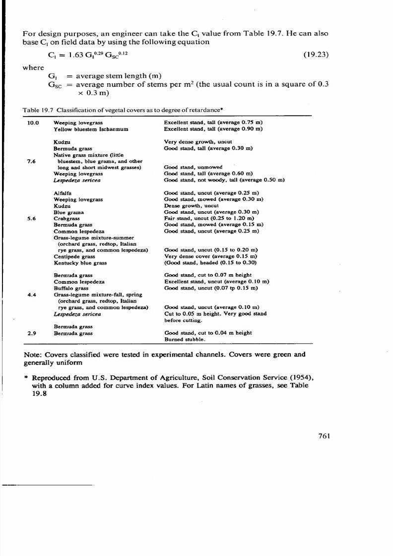
Fo r design purposes, an engineer can tak e the C, value from T able 19.7. He can also

base C, on field da ta by using the following equa tion

C ,= 1.63G” Gsco.12 (19.23)

where

G,Gsc =average nu mb er of stems per m 2 (the usual co un t is in a square of 0.3

= average stem length (m )

x 0 . 3m)

Table 19.7 Classificationof vegetal covers as to degree of retardance*

10.0

7.6

5.6

4.4

2.9

Weeping lovegrass

Yellow bluestem Ischaemum

Kudzu

Bermuda grass

Native grass mixtu re (little

bluestem, blue grama, and otherlong and short midwest grasses)

Weeping lovegrass

L.espedeza scriceo

Alfalfa

Weeping lovegrass

Kudzu

Blue grama

Crabgrass

Bermuda grass

Common lespedeza

Grass-legume mixture-summer

(orchard grass, redtop, Italianry e grass, and common lespedeza)

Centipede grass

Kentucky blue grass

Bermuda grass

Common lespedeza

Buffalo grass

Grass -legum e mixture-fall, sprin g

(orchard grass, redtop, Italian

ry e grass, and common lespedeza)

Lespedeza sericca

Bermuda grass

Bermuda grass

Excellent stand, tall (average 0.75 m)

Excellent stand, tall (average 0.90 m)

Very dense growth, uncut

Good stand, tall (average 0.30 m)

Good stand, unmowed

Good stand, tall (average 0.60 m)

Good stand, not woody, tall (average 0.50 m)

Good stand, uncut (average 0.25 m)

Good stand, mowed (average 0.30m)

Dense growth, uncut

Good stand, uncut (average 0.30m)

Fair stand, uncut (0.25 to 1.20 m)

Good stand, mowed (average 0.15 m)


Good stand, uncut (0.15 to 0.20 m)

Very dense cover (average 0.15 m)

(Good stand, headed (O. 15 to 0.30)

Good stand, cut to 0.07 m height

Excellent stand, uncut (average 0.10 m)

Good stand, uncut (0.07 tp 0.15 m)


Cut to 0.05 m height. Very good stand

before cutting.

Good stand, cut to 0.04 m height

Burned stubble.

Note: Covers classified were tested in experimental channels. Covers were green andgenerally uniform

* Reproduced from U.S. Department of Agriculture, Soil Conservation Service (1954),

with a column added for curve index values. For Latin names of grasses, see Table19.8

76 1



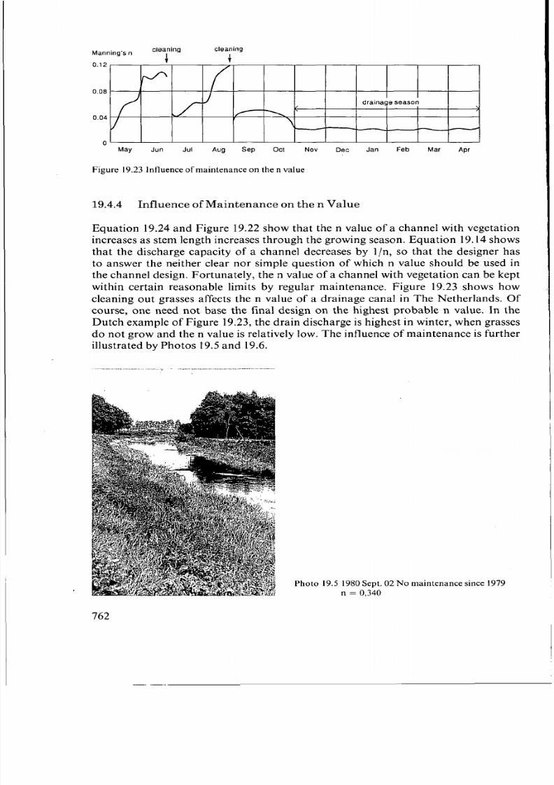
Ma y J un J ul Aug Sep Oc t No v Dec Jan Feb Mar Apr

Figure 19.23 Influence of maintenance on t h e n value

19.4.4 Influence of Maintenance on th e n Value

Equation 19.24 and Figure 19.22 show that the n value of a channel with vegetationincreases as stem length increases through the growing season. Equation 19.14 shows

that the discharge capacity of a channel decreases by l/n, so that the designer hasto answer the neither clear nor simple question of which n value should be used in

the channel design. Fortunately, the n value of a channel with vegetation can be kept

within certain reasonable limits by regular maintenance. Figure 19.23 shows howcleaning out grasses affects the n value of a drainage canal in The Netherlands. Ofcourse, one need not base the final design on the highest probable n value. In theDutch example of Figure 19.23, the drain discharge is highest in winter, when grassesdo not grow and the n value is relatively low. The influence of maintenance is further

illustrated by Photos 19.5 and 19.6.

Photo 19.5 1980Sept. 02 N o maintenance since 1979

n = 0,340

762



P h o t o 19.6 1980 Dec. 18 Some t ime after maintenance

n =0.040 (Courtesy University of

Agriculture, Wageningen)

19.4.5 Ch a n n e l s w i th Co mp o u n d S e c t io n s

The cross-section of a channel may consist of several subsections, each subsection

having a different roughness. F or exam ple, a main dra in with a dry-season base flowand wet-season floods may have a compound cross-section like the one in Figure

19.24A. Th e shallow parts of the channel are usually rougher than the deeper centralpa rt. In such a case, it is a good idea to apply Manning’s equ ation separately to eachsub-area (A,, A,, and A3). The total discharge capacity of the channel then equals

the sum of the discharge capacities of the su b-areas.Th e same can be said ab ou t trapezoidal canals, like the one in Figure 19.24B, that

have thick vegetation o n the banks while the earthen b ott om remains clear. Th e flow

through the areas m arked A, should then be calculated using a higher n value than

the one used to calculate the flow through the area ma rked Ah.We ca n use the following

relations

2A, = (zY’) +0.2 (by)

P, =2 y J z z s 1

AhR -b - K

(19.24)

(1 9.25)

( 1 9.26)

(19.27)

(19.28)

( 1 9.29)

763

normal depth

Documents