Normal Distribution

• A particular family of distributions (“bell curve)– Where once you know the mean and the standard deviation

– you know the distribution

– Ae(x-<x>)2 gives a bell shaped curve

• Which many real world distributions approximate– And which has characteristics that are known and useful

– About 68% within one stdev, 95% within two, 99.7% within three

• If you know the mean IQ is 100 and the stdev is 15, just how special is your IQ 150 kid?

• Z score table is the continuous version of that rule– Z score is the number of standard deviations from the mean.

– Table tells you how likely it is that the Z score is no higher than that

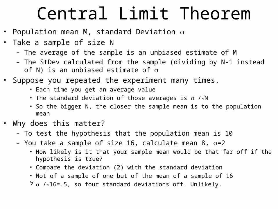
Central Limit Theorem• Population mean M, standard Deviation • Take a sample of size N

– The average of the sample is an unbiased estimate of M

– The StDev calculated from the sample (dividing by N-1 instead of N) is an unbiased estimate of

• Suppose you repeated the experiment many times.• Each time you get an average value• The standard deviation of those averages is /N • So the bigger N, the closer the sample mean is to the population mean

• Why does this matter?– To test the hypothesis that the population mean is 10

– You take a sample of size 16, calculate mean 8, =2• How likely is it that your sample mean would be that far off if the hypothesis is true?• Compare the deviation (2) with the standard deviation• Not of a sample of one but of the mean of a sample of 16 /16=.5, so four standard deviations off. Unlikely.

Rents paid by law students at SCU• Take a sample of 100

– First deduce standard deviation of the population from the sample

• Calculate the mean of the sample: <rent>• For each rent, calculate (rent - <rent>)2

• Add up and divide by 99 (why 99 not 100?)• The square root is your estimate of the standard deviation of the

population: • Which measures how much rents vary from student to student

– Then deduce the standard deviation of the mean• Standard deviation of a sample of size n goes as /square root of n• For samples of that size, that’s how much their means would vary

• How likely is it that <rent> is at least that far from $1000?– The distribution of means is approximately normal– You know its standard deviation: /10– So [<rent>-$1000]/(/10) is z, consult the z table

€

x

The Calculation• Hypothesis being tested: average rent =$1000• Hypothetical numbers (from the book)

– Sample size 100– <rent>=$950 Average of the sample = $150 Standard deviation of the population (estimate) /100 = /10 = $15 Standard deviation of the mean– So Z = $50/$15 = 3.33 standard deviations above

• Two tailed test; why?– Z table shows .995 below 3.33, .005 below -3.33– So .99 between the two values– So .01 probability that <x> at least that far from $1000 by

chance

What does it mean?• If the average rent for all students is $1000

– There is one chance in 100– That a sample of 100 rents would have a mean– At least $50 higher or lower– Significance at .01--very strong result

• That does not mean either– That the probability the rent is actually $1000 is .01– How high do you think it is?– Or that the difference of the rent from $1000 is

significant in the normal sense--i.e. large• Suppose the population were San Jose, n=10,000• Z=3.33 represents a mean how far from $1000?

Hypothesis Testing

• The basic logic of confidence results– You have a null hypothesis—this coin is fair

– You have a sample—say the result of flipping the coin ten times. 7 heads.

• You want to decide whether the null hypothesis is true– In the background there is an alternative hypothesis

– Which is relevant to how you test the null hypothesis

– For instance—this coin is not fair, but I don't know in which direction

• You ask: If the null hypothesis is true, how likely is a result at least this far from what it predicts in the direction the alternative predicts– For example, if the coin is fair

– How likely is it that the result of my experiment would be this far from 50/50?

• Suppose the answer is that if the coin is fair, the chance of being this far off 50/50 is less than .05 (i.e. 5%)

• You then say that the null hypothesis is rejected at the .05 level

To Restate• Confidence level tells you how strong this piece of

evidence against the null hypothesis is– but not how likely the null hypothesis is to be true– analogously, it might be that a witness identification has

only one chance in four of being wrong by chance– but if you have a solid alibi, you still get acquitted

• "Statistically significant" doesn't mean "important" it means "unlikely to occur by chance"– I take a random coin and flip it 10,000 times– the result will prove it isn't a fair coin to a very high level

of significance

• Even if it is "unfair" only by .501 vs .499 probability

This is all sampling error• Sampling error can be calculated, but..

– Other forms of error may be more important– So "the margin of error is" may be misleading

• Consider DNA tests– "The chance that the defendant's DNA would match

this closely is less than one in a hundred million"– May be a true statement about sampling error– But there have been far more mistaken results than

that number suggests• Rates of human error are much higher than that• As are rates of deliberate fraud

• Think of sampling error as a lower bound

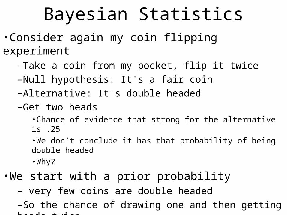
Bayesian Statistics•Consider again my coin flipping experiment

–Take a coin from my pocket, flip it twice–Null hypothesis: It's a fair coin–Alternative: It's double headed–Get two heads

•Chance of evidence that strong for the alternative is .25•We don’t conclude it has that probability of being double headed•Why?

•We start with a prior probability– very few coins are double headed–So the chance of drawing one and then getting heads twice–Is much lower than the chance of drawing a fair coin and getting heads twice–So the latter is what probably happened

Done formally• Suppose one coin in 1000 is double headed

– Probability of pulling one from my pocket: .001– If it is double headed, prob of two heads: 1– So joint probability--that both happen--is .001

• 999 in 1000 coins are (approximately) fair– P of pulling a fair coin from pocket: .999– If fair, p of two heads: .25– Joint probability is .25x.999=.24975

• We know one of these two things happened– Relative probability is .001/.24975=aprox 1/250– So odds about 250 to 1 that the coin is fair

• This is Bayesian statistics as opposed to classical statistics

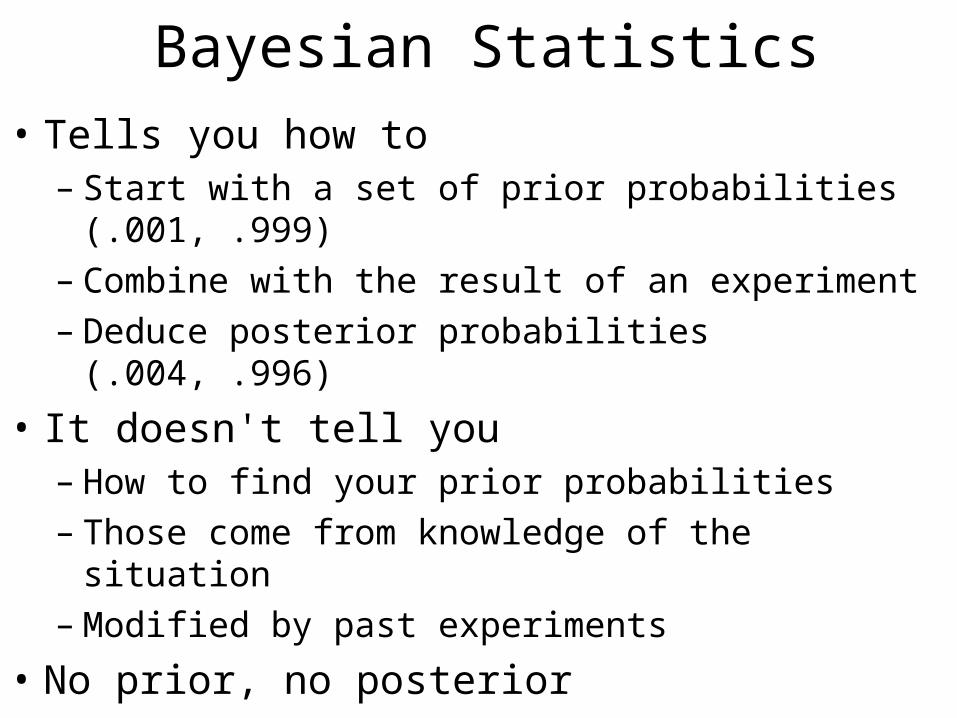
Bayesian Statistics

• Tells you how to– Start with a set of prior probabilities (.001, .999)– Combine with the result of an experiment– Deduce posterior probabilities (.004, .996)

• It doesn't tell you– How to find your prior probabilities– Those come from knowledge of the situation– Modified by past experiments

• No prior, no posterior

How to Lie: Part 2• Report sampling error as if it was all error• Report confidence result with meaning reversed

– The theory that the firm didn't discriminate against women– Can be rejected at the .05 level– So the odds are twenty to one that it did

• Report selected result– This study found our product clearly worked– And we aren't telling you about the other 19 studies– And this happens even without trying

• Academic version: if you don't get results you can't publish• Popular version: the most striking result gets the press• Both can cause unintentionally misleading results, but also

– Are incentives to deliberately distort results

– Since getting published and getting press may be the objectives

You can also just lie

• Statistics prove that

• 95% of quoted statistics are invented

Including this one

Multivariate statistics• Each item (person, country, state, year) has two characteristics

– How are they related to each other?

– Why?

• Descriptive approach: Scatterplot– Approximate linear relationship. But note

– The plot might show you more complicated things, that calculating the correlation coefficient would miss.

– Humans come with very good pattern recognition built in.

Correlation Coefficient• We have two characteristics, each associated with individuals in a

population– Height and weight of people– Rainfall and average temperature of years– Income and Lsat score

• Which could be parental income and student LSAT score or• Entering LSAT and later income as a lawyer

• We want to know how the two are related– When height is above average, is weight above average? (Probably)– Do cool years have more rainfall?

• Correlation coefficient is a measure of how consistently– When one variable is above its average, the other is above its (positive

correlation)– Or when one is above, the other is below (negative)– 1 is perfect correlation--if you plot them they are on a straight line, slopes up– -1 is perfect negative correlation--straight line, slopes down– 0 is no correlation--but not necessarily no relationship.

• The first one you would get a positive correlation coefficient—what would you miss?

• The second one, near zero correlation. But …

• The scatter plot shows the pattern

• Summary– The coefficient is from –1 to 1

– Sign tells you whether larger than average values of one variable imply larger than average values of the other (+) or smaller (-)

– The magnitude tells you how perfect the relation is, not the slope.

• Which of these has the higher correlation coefficient?

• This is the same point I made earlier about significance– Statistically significant means we are sure the effect is there

– It says nothing about how large it is

– 550 heads/450 tails is much more significant evidence of unfairness than

– 3 heads/1 tail

Mathematical Definition• For each value of the first variable, calculate how many standard deviations it is

from the mean--+ if greater than mean, - if less• For each observation (person, state, …) multiply that figure for the first variable

times that figure for the second• Average over all observations

– (except you divide by n-1 instead of by n in averaging)– for the same reason we did it earlier—sample slightly exaggerates the correlation for the

population.– I think

• Why this makes (some) sense• If above average values of X occur for the same observation as above average

values of Y, the product is positive• If below go with below, the product is still positive—negative times negative is

positive• So if the two variables move together, get a positive correlation coefficient• If they move in opposite directions, above average of one go with below average of

the other, so + times – or – times +, which gives negative• Average lots of negative numbers, get a negative correlation coefficient

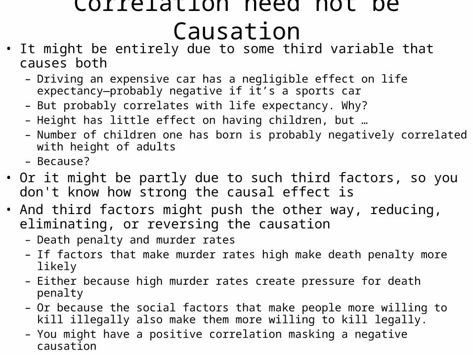
Correlation need not be Causation• It might be entirely due to some third variable that causes both

– Driving an expensive car has a negligible effect on life expectancy—probably negative if it’s a sports car

– But probably correlates with life expectancy. Why?– Height has little effect on having children, but …– Number of children one has born is probably negatively correlated with height

of adults– Because?

• Or it might be partly due to such third factors, so you don't know how strong the causal effect is

• And third factors might push the other way, reducing, eliminating, or reversing the causation– Death penalty and murder rates– If factors that make murder rates high make death penalty more likely– Either because high murder rates create pressure for death penalty– Or because the social factors that make people more willing to kill illegally also

make them more willing to kill legally.– You might have a positive correlation masking a negative causation

And Causation may not lead to correlation

Causation, Correlation and Prediction• Correlation can be used to predict• "if the state has a death penalty, it probably has a high

murder rate"– doesn't depend on which causes which

– or whether there is a third factor causing both

• but if you have the causality wrong, you might get the prediction wrong– because you are missing other relevant evidence

– taller adults are less likely to have born children than shorterbut taller females aren't.You also might get the policy wrong:

Dying correlates with being in the hospital. In order not to die …

What if death penalty correlates positively with murder rate?

Linear Regression• instead of measuring how close to a line the points come (correlation

coefficient)• you try to estimate the line they come closest to• which requires some definition of "close."

– You want to count both being too high and too low as errors– So the difference between point and line wouldn't work– Instead use the square of the difference—positive each way– Find the line that minimizes the summed square deviation.

•Unlike the correlation coefficient, this one measures the size of the effect•y= A+Bx

–A is the intercept—where the line crosses the vertical axis–B is the slope—how much the line goes up for each unit it goes out

Goodness of Fit• By convention, X (horizontal) is the independent variable, Y

(vertical) the dependent: Y=A + BX

• Simplest "prediction" is that Y always equals its average value

• How much of the departure from that does the regression explain?

•

• TSS is the sum of squared residuals from the average

€

R2 ≡TSS − SSR

TSS=

Total Sum of Squares - Sum of Squared Residuals

Total Sum of Squares

€

TSS = Y1 − Y ( )2

+ Y2 − Y ( )2+ Y3 − Y ( )

2+...

Y = Average value of Y

€

SSR = Y1 − A + BX1( )( )2

+ Y2 − A + BX2( )( )2

+ Y3 − A + BX3( )( )2+...

Because A + BX1( ) is the predicted value of Y1

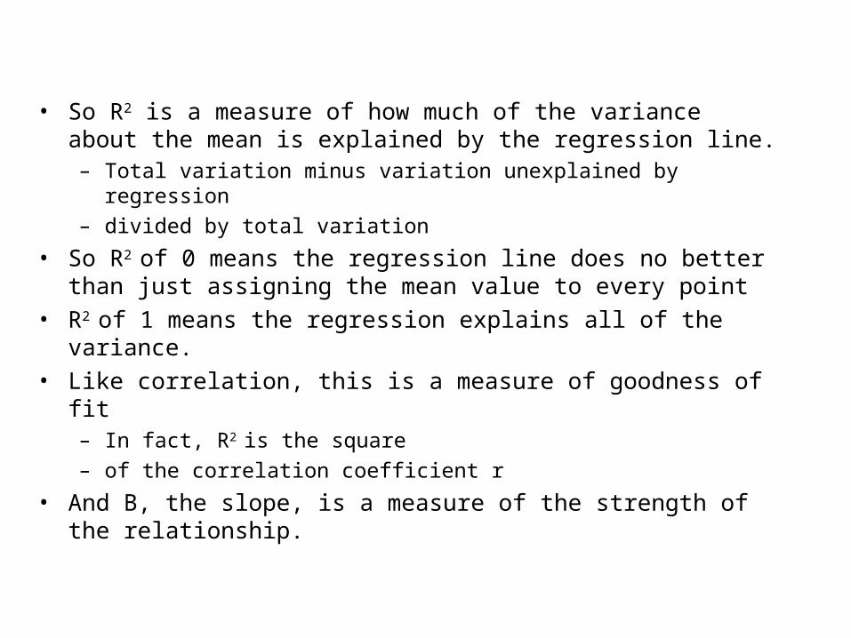
• So R2 is a measure of how much of the variance about the mean is explained by the regression line. – Total variation minus variation unexplained by regression

– divided by total variation

• So R2 of 0 means the regression line does no better than just assigning the mean value to every point

• R2 of 1 means the regression explains all of the variance.

• Like correlation, this is a measure of goodness of fit– In fact, R2 is the square

– of the correlation coefficient r

• And B, the slope, is a measure of the strength of the relationship.

Residuals

• If you plot the residuals from a regression--distance above or below the line

• It will show you which points don't fit the pattern• In exploratory statistics, you might want to color points in ways

reflecting other characteristics– Men/women– Blacks/whites– Northern states/Southern states– CEO's relatives/non-relatives– And see if any such coloring explained the pattern

• In the book's example, Mary Starchway is both an outlier and an influential observation– Outlier because her wage is much higher than anybody else's– Influential observation because she is far off the experience/wage

regression line– Does the first necessarily imply the second?

Limitations of Linear Regression• There might be a close relationship that isn't linear

• there are procedure analogous to linear regression for dealing with the first case– Instead of plotting Y=A+BX you might plot– Y=A+BX+CX2 for example– Giving something like that if B<0 and C>0

• The second case strongly suggests that we need more than two variables– Y is determined by X, and also by– Whatever it is that distinguishes the two lines

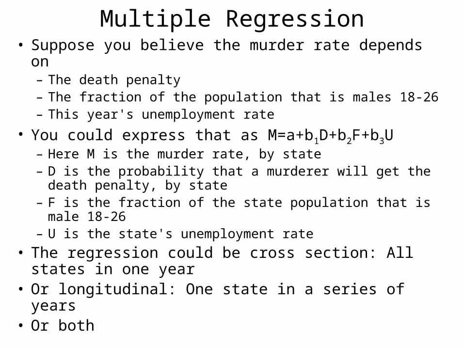
Multiple Regression• Suppose you believe the murder rate depends on

– The death penalty– The fraction of the population that is males 18-26– This year's unemployment rate

• You could express that as M=a+b1D+b2F+b3U– Here M is the murder rate, by state– D is the probability that a murderer will get the death penalty,

by state– F is the fraction of the state population that is male 18-26– U is the state's unemployment rate

• The regression could be cross section: All states in one year

• Or longitudinal: One state in a series of years• Or both

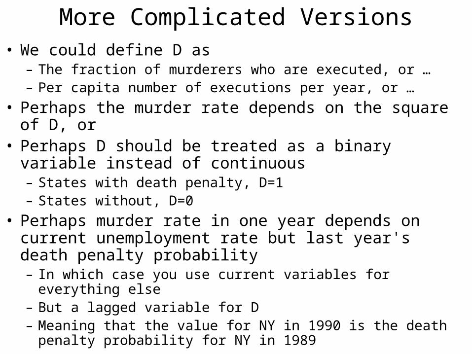
More Complicated Versions• We could define D as

– The fraction of murderers who are executed, or …– Per capita number of executions per year, or …

• Perhaps the murder rate depends on the square of D, or • Perhaps D should be treated as a binary variable instead of

continuous– States with death penalty, D=1– States without, D=0

• Perhaps murder rate in one year depends on current unemployment rate but last year's death penalty probability– In which case you use current variables for everything else– But a lagged variable for D– Meaning that the value for NY in 1990 is the death penalty

probability for NY in 1989

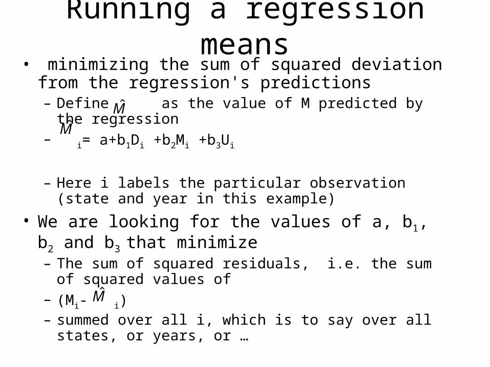
Running a regression means• minimizing the sum of squared deviation from the

regression's predictions– Define as the value of M predicted by the regression–

i= a+b1Di +b2Mi +b3Ui

– Here i labels the particular observation (state and year in this example)

• We are looking for the values of a, b1, b2 and b3 that minimize– The sum of squared residuals, i.e. the sum of squared

values of– (Mi- i) – summed over all i, which is to say over all states, or years,

or …

€

ˆ M

€

ˆ M

€

ˆ M

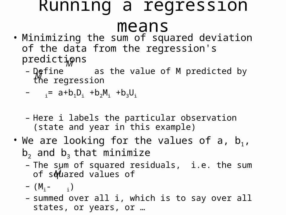
Running a regression means• Minimizing the sum of squared deviation of the data

from the regression's predictions– Define as the value of M predicted by the regression–

i= a+b1Di +b2Mi +b3Ui

– Here i labels the particular observation (state and year in this example)

• We are looking for the values of a, b1, b2 and b3 that minimize– The sum of squared residuals, i.e. the sum of squared

values of– (Mi- i) – summed over all i, which is to say over all states, or years,

or …

€

ˆ M

€

ˆ M

€

ˆ M

Significant Coefficients

• Regression results shows some coefficient>0– We want to know how sure we are it is true– For instance, that whites get paid more than blacks– Controlling for all other relevant factors

• We use a t test which is– Analogous to the significance tests we have done– Both in how it works and what it means– t = coefficient/its standard error– I.e. how big it is relative to how uncertain

• Look up the corresponding confidence level– On a t table--like a z table, but with one complication– Degrees of freedom

Degrees of freedom• Suppose I have only two data points

– (x1, y1) (x2,y2)– And do a simple regression: y=a+bx– How well will I fit the data?

•Perfectly•You can always draw a straight line through two points

•The result generalizes•With n parameters you can fit n data points•Whatever the relation among them is•So only fitting more points than that counts as evidence•Which is what the degrees of freedom take account of

Give me enough parameters and I’ll fit the skyline of New York

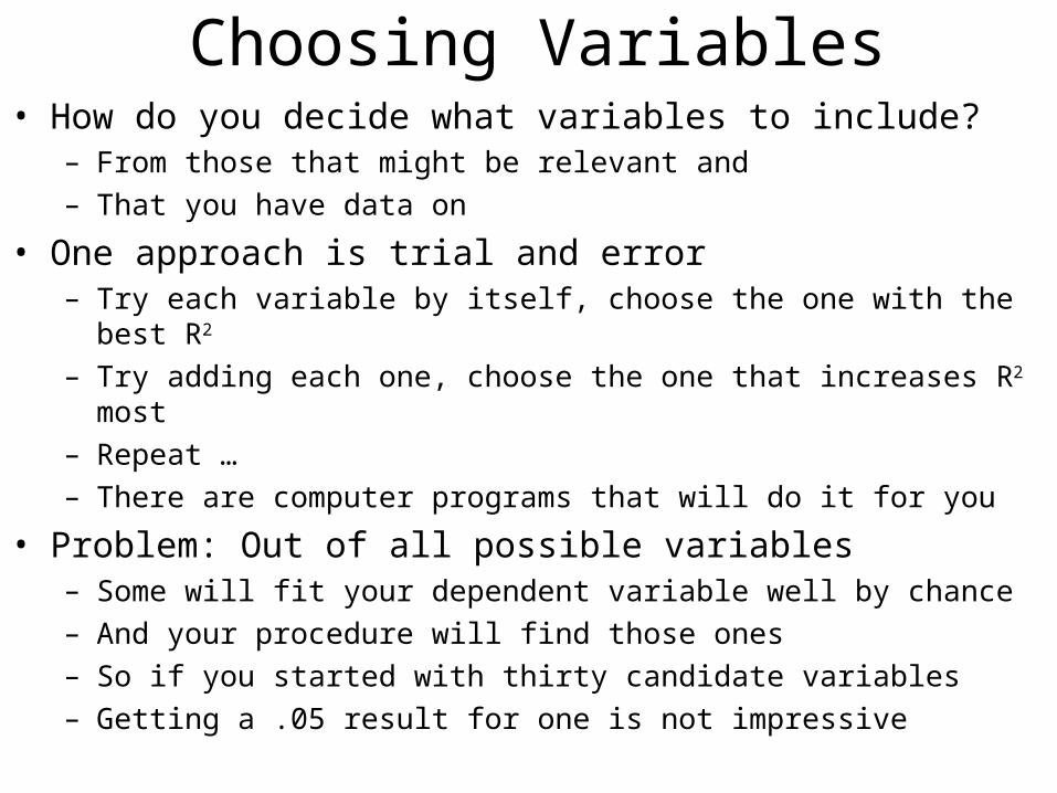
Choosing Variables• How do you decide what variables to include?

– From those that might be relevant and– That you have data on

• One approach is trial and error– Try each variable by itself, choose the one with the best R2

– Try adding each one, choose the one that increases R2 most– Repeat …– There are computer programs that will do it for you

• Problem: Out of all possible variables– Some will fit your dependent variable well by chance– And your procedure will find those ones– So if you started with thirty candidate variables– Getting a .05 result for one is not impressive

Problems or How to Cheat• All the usual ways, such as …

– Misstate the meaning of significance– Use a biased sample– Select which experiments to report– Use unreliable data

• Plus some brand new ways– Plaintiff claims aspartame causes cancer

• My regression found no significant relation

• Independent variables: age, gender, use of diet drinks, aspartame consumption

– Defense claims his prostate medicine doesn’t shorten life• My regression shows a strong correlation

• Independent variables: state of residency, race, use of prostate medicine

• Dependent variable: Age at death

Collinearity problem• Significance calculation is based on

– How much better you fit the data by adding this variable

– Which depends on what other variables are there

– Suppose you include both temperature F and temperature C

– How significant do you think either will be?

• t test is asking how many standard deviations out the coefficient is– Which depends on how precisely you know the coefficient

– In my case, if you have one, the coefficient on the other could be anything• Heating oil consumption = A +B(temp F) + C(temp C)• Do you see why?

• The same problem exists in less extreme cases– Adding a variable that correlates closely with another

– Decreases the other’s significance, because …

– The new one can explain most of the same variation.

Omitted Variable Problem

• You want to prove that X (prostate medicine) causes Y (shorter life)

• You leave out a variable that correlates with both– Prostate medicine is only used by men– Men have shorter life expectancies than women– So don’t include gender in your regression

• Your independent variable X– Now seems to be predicting Y, because– X predicts gender, which predicts Y

Furman v Georgia • The case that (temporarily) abolished the death penalty• Also a famous use of statistics

– Data on all capital cases– Commonly said to have shown discrimination against blacks

• Control for race of victim– black who killed a black more likely to be executed than– White who killed a black. Ditto if victim was white. But …– Killer of a black much less likely to be executed than of a white– And blacks mostly kill blacks, whites whites– Which is why black killers less likely to be executed

• It was indeed evidence of racial discrimination– Slight discrimination against black defendants, race of victim held

constant– Large discrimination against black victims, race of killer held constant

– But … black defendants had a lower probability of execution than white defendants!

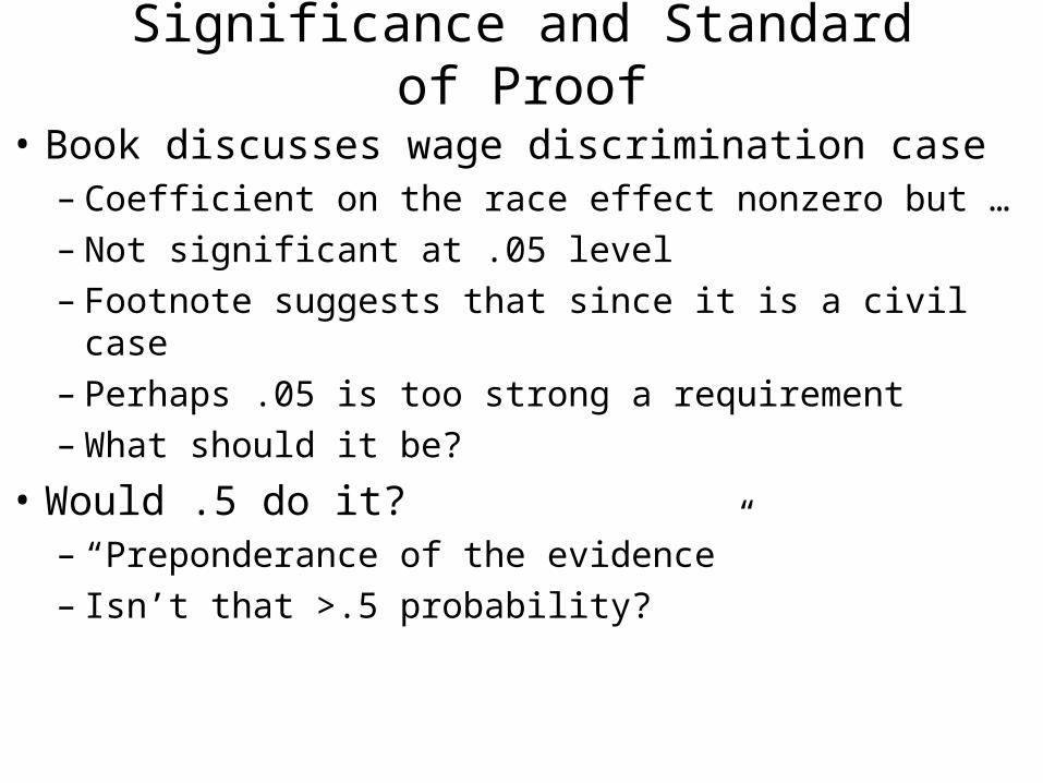
Significance and Standard of Proof

• Book discusses wage discrimination case– Coefficient on the race effect nonzero but …– Not significant at .05 level– Footnote suggests that since it is a civil case– Perhaps .05 is too strong a requirement– What should it be?

• Would .5 do it?– “Preponderance of the evidence”– Isn’t that >.5 probability?

Statistics and the Law School• You want to raise the bar passage rate

• You have data on all students for the past ten years– Information on them when they applied– What courses they took, grades they got– Bar exam outcomes

• How might you use it?– What questions would you ask?– How could statistics answer them?– How could you use the information?

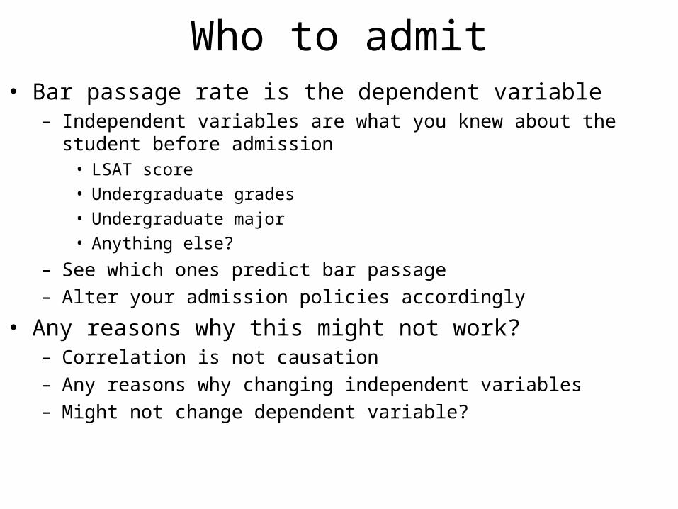
Who to admit• Bar passage rate is the dependent variable

– Independent variables are what you knew about the student before admission

• LSAT score

• Undergraduate grades

• Undergraduate major

• Anything else?

– See which ones predict bar passage– Alter your admission policies accordingly

• Any reasons why this might not work?– Correlation is not causation– Any reasons why changing independent variables– Might not change dependent variable?

Class record• Regress bar passage rate on

– What classes student took– What grades he got on them

• Suppose you learn that– Students who took class X were less likely to pass– Students who took Y were more likely

• Would you raise bar passage rate by– Abolishing class X– Requiring class Y

• Suppose grades in class Z– Predict bar passage rates– Do well in Z, pass the bar, do badly, likely to fail– Drop students who did badly in Z?

• In each case, why might it not work?

How about Professors?• See how bar passage rate depends on

– Which courses the student took– From which professor– Take torts from Smith, pass the bar– From Jones, fail the bar

• Fire Jones, raise Smith’s pay or– If Jones has tenure– Have him teach something else

• More generally, rearrange who teaches what– On the basis of regression coefficients showing– The effect on bar passage rates

What do we need to know?• In each of these cases

– To decide whether using the regression results– Will let us improve outcomes– Whether correlation is probably causation– What additional information might we want?

•How were students assigned–To courses and to professors–Suppose X was a class failing students were assigned to–Or Y a class with very selective admissions, or …– Smith a notorious hard grader who weak students avoided

ABA Fails Statistics• ABA wants to include bar passage rate in deciding what law

schools to certify– What will the effect of doing this be?– Why is it a mistake?

To take account of bar passage, how should they do it?

•Bar passage rate depends on at least two things–Characteristics of the student–Characteristics of the law school he went to–Almost any school can get a student to pass the bar–If he is sufficiently smart and hard working–What matters is value added

–For a student with a given set of characteristics–How likely is he to pass the bar if he goes to this school

Use a Regression

• BPR=a+bLsat+c…– BPR = Bar Passage Rate– Lsat = student’s Lsat score– c … represents other relevant student characteristics

• The higher a and b, the better the school– Because the more likely to get a given student– To pass the bar

• Some schools may do well with low Lsat students, some with high– So report a, b, c …– And let the student calculate the probability that he will pass– If he goes to that school

• Bar association could decide to certify any school– That does relatively well for some– Substantial group of students– Including schools that are good for weak students

Statistics Exercises• On the syllabus, for practice

• Do the calculations with numbers

• We will discuss them next class

Statistics: You should know• Ways of displaying and summarizing data

– Histogram, median, mean– Some idea of what which are useful for

• What terms such as "significant" and "confidence interval" mean– Testing a conjecture– Null hypothesis/alternative hypothesis– One tailed and two tailed tests– Normal distribution, central limit theorem, z

• What a correlation coefficient shows• What a regression result, single or multiple, means

– Coefficients and– Measures of significance (R2, t)

• What can go wrong– How statistical results can be presented to mislead– How statistics can mislead, intentionally or not

You are not expected to• Be able to do a regression

– If you ever need to, find the relevant software– Or get a statistician to do it for you

• Prove things• Give precise definitions

– Of correlation coefficient– Least squares fit– R2

– But you should understand about what they mean

• You need to understand enough – Not to be fooled– To know what questions to ask– And about what the answers mean

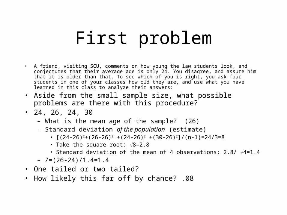
First problem• A friend, visiting SCU, comments on how young the law students look, and conjectures that their

average age is only 24. You disagree, and assure him that it is older than that. To see which of you is right, you ask four students in one of your classes how old they are, and use what you have learned in this class to analyze their answers:

• Aside from the small sample size, what possible problems are there with this procedure?

• 24, 26, 24, 30– What is the mean age of the sample? (26)– Standard deviation of the population (estimate)

• [(24-26)2+(26-26)2 +(24-26)2 +(30-26)2]/(n-1)=24/3=8• Take the square root: 8=2.8• Standard deviation of the mean of 4 observations: 2.8/ 4=1.4

– Z=(26-24)/1.4=1.4

• One tailed or two tailed? • How likely this far off by chance? .08