normal products of self-adjoint operators and self
TRANSCRIPT

Normal Products of Self-adjoint Operators and Self-adjointness of the Perturbed Wave
Operator on L 2 (R)
Mohammed Hichem Mortad
Doctor of Philosophy in Mathematics. The University of Edinburgh.
July 2003
(•

Abstract
This thesis contains five chapters. The first two are devoted to the background which consists
of integration, Fourier analysis, distributions and linear operators in Hilbert spaces.
The third chapter is a generalization of a work done by Albrecht-Spain in 2000. We give a
shorter proof of the main theorem they proved for bounded operators and we generalize it to
unbounded operators. We give a counterexample that shows that the result fails to be true for
another class of operators. We also say why it does not hold.
In chapters four and five, the idea is the same, that is to find classes of unbounded real-valued
Vs for which LI + V is self-adjoint on D(Li) where LI is the wave operator.
In chapter four we consider the wave operator defined on L 2 (R2 ) while in chapter five we
do the case L 2 (R"), ri > 3. Throughout these two chapters we will see how different the
Laplacian and the wave operator can be.

Declaration of originality
I hereby declare that the research recorded in this thesis and the thesis itself was composed and
originated entirely by myself in the School of Mathematics at The University of Edinburgh.
MOHAMMED HTC14EM MORTAD
111

Acknowledgments
First, there is someone who deserves the best thanks. A very famous mathematician and a very
nice person that is my supervisor Professor Alexander M. Davie who has helped me to achieve
this work with very good hints and bright ideas.
I also should be grateful to the Algerian Government that has provided me with a full schol-
arship to allow me to study here in the United Kingdom and at this well-known and famous
University.
I also thank my family back in Oran (in Algeria) especially my parents, who even far away,
have always been with me with their moral support.
iv

Contents
Declaration of originality .............................iii Acknowledgments ................................iv Contents . . . . . . . . . . . . . . . . . . . . . . . . . . . . . . . . . . . . . . v
0 Introduction 1
1 Integration, Fourier analysis and distributions 3 1.1 Integration ..................................... 3
1.1.1 LP spaces ................................. 3 1.1.2 LP Spaces ................................ 6
1.2 The Fourier transform ............................... 9 1.2.1 The L'-Fourier transform ........................ 9 1.2.2 The L 2 -Fourier transform ........................ 10 1.2.3 The LP-Fourier transform for 1 <p < 2................. 11
1.3 The space BMO ................................. 12 1.4 Distributions ................................... 13
1.4.1 Distributional derivatives ......................... 14 1.4.2 Multiplication of distributions by C'-functions ............. 14
1.5 Sobolev spaces .................................. 15 1.5.1 The space Hl(Rn1) ............................ 15 1.5.2 Fourier characterization of H'(R) .................... 15
2 Linear operators in Hubert spaces 17 2.1 Hilbert spaces ................................... 17 2.2 Bounded linear operators on Hilbert spaces ................... 18 2.3 Unbounded linear operators on Hubert spaces .................. 20
2.3.1 Domains, graphs, extensions and adjoints ................ 20 2.3.2 Symmetric and self-adjoint operators .................. 22 2.3.3 The basic criterion for self-adjointness .................. 23 2.3.4 Normal operators ............................. 25 2.3.5 Spectral theory of linear operators .................... 25 2.3.6 The spectral theorem for normal operators ................ 26
2.4 Perturbation of unbounded linear operators ................... 28 2.5 Limit point-limit circle case ............................ 29
3 An application of the Putnam-Fuglede theorem to normal products of self-adjoint operators 32 3.1 Introduction ....................................32 3.2 Normal products of self-adjoint operators ....................32
3.2.1 Bounded normal products of self-adjoint operators ...........32 3.2.2 Unbounded normal products of self-adjoint operators ..........33
3.3 A counterexample .................................38 3.4 What went wrong? ................................42
v
Contents
4 Self-adjointness of the perturbed wave operator on L 2 (R2 ) 47
4.1 Introduction ....................................47
4.2 First class of self-adjoint 0 + V ......................... 48
4.3 M12 and the space BMO ............................. 53
4.4 Counterexamples .................................59
4.5 Open problems ..................................66
5 Self-adjointness of the perturbed wave operator on L 2 (R), n > 3 68
5.1 Introduction ....................................68 5.2 A class of self-adjoint 0 + V on L 2 (R"), n > 3 ................68
5.3 Counterexamples: .................................84
5.4 Open problems ..................................86
5.5 Conclusion ....................................88
References 89
Vi

Chapter 0 Introduction
The main subject treated in this thesis is linear operators on Hubert spaces (especially un-
bounded ones). We devote two chapters to the background that consists of different subjects
such as L"- spaces, distributions, Fourier analysis, interpolation theory of operators, linear
bounded and unbounded operators and perturbation theory.
In Chapter three we generalize work done by Albrecht and Spain [1] who gave a condition
that forced a product of two self-adjoint operators to be self-adjoint whenever it was normal.
The generalization we make here is that the same condition allows us to prove the same thing
for unbounded operators. We also give a shorter proof than theirs in the bounded case and
a counterexample showing that the condition may fail to make a product of two self-adjoint
operators, when it has a normal closure, essentially self-adjoint. In the last section we say why
the proof may fail to work if we want to adapt it to the counterexample cited above.
The generalization and the counterexample form a paper by the author [2] which is due to be
published in the October 2003 issue of the Proceedings of the American Mathematical Society
In Chapters four and five we study the self-adjointness of the perturbed wave operator E + V
(the wave is a hyperbolic operator). We emphasize the word hyperbolic inasmuch as a lot of
work has been done in the case of the perturbed elliptic operator mainly the perturbed Laplacian
which is important in quantum mechanics (for a more detailed treatment of the subject we
recommend [3]).
Since it may be quite hard to solve
(D+V)f=±if ... (E)
in L 2 (R) and see whether it has a non-zero solution, we will be using the Kato-Rellich the-
orem to get round solving (E) explicitly. So the whole idea will be to prove estimates of the
1

Introduction
form
11111 <aIIDffI2 + blif 112
where II is a norm to be determined. All that with some interesting counterexamples.
Chapter four is devoted to the case L 2 (R2 ) and Chapter five is devoted to the case L 2 (R"),
n>3.
2

Chapter 1 Integration, Fourier analysis and
distributions
1.1 Integration
1.1.1 .0 spaces
We cite [4], [5] or [6] as references where one can find detailed proofs of the well-known results
stated in this section.
We start with LP spaces as they will be used often in this thesis. We will only consider II-'
spaces on R. We have:
Definition 1. Let 1 <p < 00. We define:
L(R) , C measurable : Ilf lip := LL if(xPdx]
For p = 00 we say that a measurable function f is in L°°(R' 1 ) if.
if II := inf{K: If(x)I :!~ Kfor almost every E R"} isfinite.
Remark 1. We usually define the elements of LP spaces as classes of equivalence rather than
functions where we say f is equivalent to g i ff - g = 0 a. e. Note that I if I Ip = 0 if and only if
f = 0 a.e. Also, "i, is a norm and LP(Rf'), equipped with this norm, is a Banach space.
Finally, it will sometimes be convenient to refer to locally integrable functions Ljoc(Rhl); f E L'j(Rn)
?f and only if f Ill < 00 for each compact set K in R. K
We now collect together some well-known inequalities in the theory of LP spaces which we
will use throughout the thesis. We begin with Holder's inequality.
Integration, Fourier analysis and distributions
Theorem 1 (Holder's inequality). Let 1 <p < oo, 1 + = 1. Let E LP (RI ), g E L" (R')
Then fg e L'(R") and
high hlfhlphlghlq.
Holder's inequality can be deduced from Young's inequality which we shall use independently
on several occasions.
Lemma 1 (Young's inequality). For all a, b > 0, if 1 + = 1, then
a b ab< — + —
p q
The case p = q = 2 in HOlder's inequality is the classical Cauchy-Schwarz inequality.
Corollary 1 (Cauchy-Schwarz inequality).
ugh' :5 11f 112119112•
The following lemma is usually called the converse of HOlder's inequality (for a proof one may
consult [4], pp. 128):
Lemma 2. Let f be a real-valued and measurable function. Let 1 <p < 00 and + 1 = 1.
Then
ii! lip = sup high, i9!Iq=1
and the supremum on the right hand side is attained.
Observe that in the previous lemma, the function f is not assumed to be in L'3 .
Remark 2. The function g (in Lemma 2) which attains the supremum can be taken to be non-
negative.
As a consequence of Lemma 2 we prove Minkowski's inequality.
Corollary 2. Let 1 < p :5 oo. Let f, g E L. Then we have:
hi! + giip Ill lip + hlghh.
4

Integration, Fourier analysis and distributions
Proof. By Lemma 2 and the triangle inequality for
If + gll p = sup{iI(f +g)hI( i : IIhIIq = 1 }
sup{fhfl 1 IIhII q = 11 +sup{IghI i : IIhII q = 1}.
Thus
If + 911P!5 IIfIIp + IIgIIp.
01
We will need the generalized Holder's inequality which is an immediate consequence of the
classical case.
Proposition 1 (Generalized Holder's inequality). Let 1 < p, q 00 and = 1 + 1 . Let
f E L' and let E Li'. Then fg ELT and
fgIIr IIfIIpIIgIIq
Definition 2. The space of infinitely differentiable functions on Rn with compact support will
be denoted by C8° (R").
Definition 3. Let f and g be two functions in L' (R"). Then we define the convolution off and
g, and we write f * g, by
(f * g) (x) =f f(x - y)g(y)dy. Rn
This integral exists almost everywhere.
Convolutions are often used in approximations. The following theorem is a well-known in-
stance of this.
Theorem 2. Let k be in L'(R), k > 0 and f k = 1. For E > 0, define k € (x) = Rn
so that f k E = 1 and 11k6111 = Ilkili. Letf E LP(R') for some 1 < p < oo and define Rn
:= k6 * f. Then
fe E L(R), 11ff lip c lIkjj j IIf lip and lim 1 1f, - f lip = 0. 6-40
If k E C°(R"), then f6 E C(R) and Df € = (Dk€ ) * f = k6 * Daf.
Integration, Fourier analysis and distributions
The last equality in the previous line is meant to be in the distributional sense (see Section 1.4.1
below).
One can easily derive from Theorem 2 the following density results.
Corollary 3. The space C8° (R") is dense in LP(R) for 1 < p < 00, and hence in particular, L1(Rh1) fl LP(Rr1) is dense in LP (R").
Definition 4. Let A > 0 and EA denote the distribution function off, i.e.,
EA={xER:If(x)I>Al.
Proposition 2. Let f e LP(R' 1 ). Then we have
00
lif lip = 10 A'EdA.
Proof. Using
PEA l =fdx,
we have
pZ 00
A''lEAldA = f A1'-1 f dxdA.
Since everything is positive one obtains by using Fubini's Theorem,
/ foo
p / A 1 1EA IdA = çL If(x)I AP_ 1 dA) dx = f lf(x)ldx = lPfll.
Rn Jo
R'
(Here we have used to denote Lebesgue measure but we will also use it to denote the usual
norm in R. The context will always be clear.) D
1.1.2 LP. Spaces
For references we cite [3] or [7].
Weak I)' spaces L, being larger than the LP spaces, are often used when a particular object
fails to be in L.
31
Integration, Fourier analysis and distributions
Definition 5. A function f on R is said to be in weak-L, written f E L,, if there is a
constant C < oo such that
l{x : lf(x)I > t} I < Ctfor all t> 0.
1ff E L, we write
If Ilp,w = sup(tP{x: lf(x)I > t}.
Notice that is not a norm since it does not satisfy the triangle inequality. However, when
p> 1, Lpw carries the structure of a Banach space with a norm which is equivalent to
Remark 3. Any function in LP is in LPW and we have:
IIflip,w If lip.
In fact for any t> 0,
iflI >— f lf(x)Idx > I{x: I f(x)I > t}lt. If I>t
The inequality tI{x : lf(x)l > t} if li is called Chebyshev's inequality.
Example 1. A typical example is the function lxl'. Then l{x : I f(x)I > t}I = cntP where
c is the volume of the unit ball in R. Thus f e L(R) but f is not in LP (R').
We come now to a result which will be important for us.
Theorem 3. Let r> 1. If r <p < s and f E L' fl L 3 then f E L and W w'
Ill lip :!~ all! IIr,w + bIll ii,w (1.1)
where the constants a and b depend on p, r and s.
Proof Let f E L(R). By definition
IEA I = If E R' : If(x)i ~! A}I <cAT
'A

Integration, Fourier analysis and distributions
Also when f E L, (R')
IEl = l{x E W': If(x)I ~:
All < cA
(here c3 and Cr denote iis,w and respectively). So
P00 1 00 II tiip IIJIILP(R) =PJ \P_' IEAIdA=PJ A''lEAid+p / A' ' iEAldA
0 0 J1
~ PC, fo AP_r_ld+pCsI°°P_s_dA
Hence
ill lipLP(Rn) PCr1 A — 1 1 1A 100
+pc3 l Lp — rj o Lp—si 1
which is finite if r <p < s. Therefore
lifllPRfl) '
llfil+ sp l 1 p — r
Thus
fIILP(Rn) IifilW + ëlifIiw (1.2)
for some constant ö depending on p, r and s.
Now we proceed to make all the powers in (1.2) equal to one. We replace f by cf where c is a
constant to be determined. We then have
S - lip Ill IILP(R") < CC llfIl7W + & P lIfIps,w•
Minimizing the quantity on the right hand side with respect to c shows that
/ s(r-p) ______
-) + ( lif i ls,W
r(s-p) ( p(r-s) •• 3p +; - (r-s)p pIlfilLP(p.j) ~ C t liflIs,w If iir,w li lIr,w
Now since the sum of the powers in each part of the right hand side is one, Young's inequality
(Lemma 1) shows
Ill lip < aIIfIlr,w + bIIfII3,,
establishing (1.1).

Integration, Fourier analysis and distributions
Finally we recall without proof the dominated convergence theorem.
Theorem 4. Let (fk)k be a sequence of measurable functions on such that:
each fk is in L 1 ;
fk -* f a. e. for some f;
there exists afunction G E L' (R") independent of k such that IfkI :5 G a.e. for all k.
Then f E L' (R") and
f k-. f(x)dx
= f urn fk(x)dx = urn f oo k—fly' R
1.2 The Fourier transform
We mention [8], [9], [7] or [3] as references in the literature for this sections.
1.2.1 The L' -Fourier transform
Definition 6. The Fourier transform off E L' (R " ) is denoted by for .Ff and defined by
I' ._,7f(X) = f(x)
=
1 (2ir) J f(t)&tdt
R
for all inR.
The inverse Fourier transform, F- 1 , is defined on L 1 (W')functions by
1 1
= (2 7r) I g(x)&tdx.
Rn
Proposition 3. Let f E L', then
the mapping f -+ f is linear and iff E L', then J1f = f a. e.
fisa bounded function and (2) hf Iii;
iff ~! 0 then If IIoo = If 11, = f(0).

Integration, Fourier analysis and distributions
Proposition 4. Let f E L' (R) and xf E L' (R). Then f is differentiable and
dt J(t) = f(t).
The proofs of Proposition 3 can be found in [7] and that of Proposition 4 can be found in [9] on
page 123.
1.2.2 The L2-Fourier transform
The Fourier transform has a natural definition on L 2 and its theory is particularly elegant on
this space. It is also important in quantum mechanics to define / for f E L 2 (R). In our work
here we will be dealing with operators that are defined on the Hubert space L 2 .
There are different routes to define the Fourier transform on L 2 . The one we will use here is
via the denseness of L' (Rn) fl L 2 (R') in L 2 (R"), see Corollary 3.
We prefer to state various aspects of the Plancherel theorem in different propositions and then
we will summarize all properties in what will be called the Plancherel theorem. First, we recall
the following facts:
The Fourier transform is defined on L' fl L 2 since L 1 fl L 2 C L' and:
L' fl L is a linear subspace of both L' and L 2 . L' fl L is a dense subspace of both L' and L 2 .
The following is the basic result.
Proposition 5. 1ff e L' fl L 2, then / E L 2 and 111112 = 111112.
Since L' fl L is dense in L 2 , Proposition 5 allows us to extend the definition of the Fourier
transform .F to all L 2 .
Proposition 6 (The Plancherel theorem). F is an isometry of L 2 , i.e. 11Ff 112 = II! II2for all
f e L.
The proofs of Propositions 5 and 6 can also be found in [7], on page 118.
10

Integration, Fourier analysis and distributions
1.2.3 The LP-Fourier transform for 1 <p < 2.
For f E LP(R), 1 < p < 2, we can decompose I = g + h where g E L 1 (') and
h E L 2 (R). Therefore we can define the Fourier transform of f by I = + ii and this is
well-defined, i.e., f is independent of the decomposition f = g + h.
Theorem 5 (Hausdorff-Young inequality). Suppose 1 < p 2, and 1 + = 1. Then the
Fourier transform is a bounded map from LP(R) to L(Rt') and
ilflIq :5 Cn,piif Il
for some constant
The proof is an easy application of the Riesz-Thorin theorem (see e.g., [3] Theorem IX. 17).
We now state a version of the well-known Sobolev embedding theorem for R" (see e.g., [3]
Theorem IX.28).
Theorem 6. Let f E L 2 (R) such that if E L 2 (R") in the distributional sense (this will be
introduced in Section 1.4.1 below). Then
if n < 3, f is a bounded continuous function and for any a> 0, there is a b, independent of
f, so that
1111100 <allfIl2 + bill 112
if ri = 4 and 2 < q < oo, then f E L(Rnl) and for any a> 0 there is a b (depending only
on q, n, and a) so that
Jfjj q < aIIzf 112 + bJIfIi2
Furthermore this estimate is false for q = oo. In fact in this case, f may be unbounded in a
neighborhood of every point (see e.g., [10] pp. 159).
if n > 5 and 2 < q then f E L(Rfl) and for any a> 0 there is a b (depending only
on q, n, and a) so that
11f Jj q < aIif 112 + blIfiI2.
11

Integration, Fourier analysis and distributions
1.3 The space BMO
The details of the following may be found in [8].
We indicate by Q c R1 any cube with sides parallel to the coordinate axes and by iQi its
Lebesgue measure. For every locally integrable f, let fQ denote the average of f on
fQ= j ff.
Definition 7. For f EL' , let to 4 denote the mean oscillation off in Q,
4 = IQIf() - fQidt. iQI
Definition 8. For f EL' C , let
Mf(x) = sup 4 r>O (x,r)
where Q(x, r) is the cube of side length r centered at x. The operator M : f -* Mf will be
called the sharp maximal operator.
Definition 9. A function f E L1'0 has bounded mean oscillation (and we say f E BMO) if
Mf E L and we set
ill 1IBMO = iiMfIl.
Remark 4. The quantity Ii IIBMQ is only a semi-norm since I lf IiBM0 = 0 if and only if
f (t) = C a. e. t. We can make BMO a norm linear space (in fact a Banach space) by passing
to equivalent classes modulo constants.
Remark 5. Every L'-function is in BMO. The converse is not true. In fact log lxi is known
to be in BMO (see e.g., [8]pp. 213).
In Proposition 27 below we will give another example of a function which is in BMO and not
in L°°.
Theorem 7 (Sharp maximal theorem). Let 1 < q p, 1 < p < oo, and suppose f E L(R) . Then f e LP (R') if and only if M O f e LP (R) and
C'IIMfIi :!~ Ilfli CIiMf lip
for some constant C.
12

Integration, Fourier analysis and distributions
A proof of the sharp maximal theorem can be found in [8] on page 220.
1.4 Distributions
Distributions is a huge subject and is treated in many textbooks from which we refer to [11],
[6] and [7].
Definition 10. Let 1 be an open subset of R1'. A sequence (fn ),, in C(l) converges in
C°() to some function f E CO' (Q) if and only if there is some fixed, compact set K c ci
such that the support of f, - f lies in K for all n and for each choice of nonnegative integers
Pi; . .. ,Pn,
( a)P /ô\Pm f0\Pi
...(-1 f-+--) ..._-) ( ,
\8x m J
as ri —* oc, uniformly on K.
Definition 11. A linear form T on C O' (Q) is a distribution if, for every sequence ( ~on )n that
converges to 0 in C'°(ci), the sequence (T(~Pn ))n tends to 0 in C.
We denote by (Co )' the set of distributions on Q.
Also the value of a distribution T on a test function W E CO , T(o), is often denoted by
(T, ) or f T(x)co(x)dx.
Example 2. The Dirac distribution Jx for x E R' is defined by
=
If EL 1 , then for any E C8°(Q) it makes sense to consider
Tf() = ff(x)(x)dx
which defines an element in (C8°(1l))'.
Since LP(Q) C 10C(Q), every LP function is a distribution.
13

Integration, Fourier analysis and distributions
1.4.1 Distributional derivatives
We now define the notion of a distributional or weak derivative. The differentiation operator of
order II = pi on (Co )' is defined as follows: If T E (Co )', set
<DT, ço > = (_ i)IPI <T, DPW > for all W E C ° .
where DP = ()P1 ()P
Since the map D : W '-p DPW from CO' to CO' is
continuous, the linear form DT defined on CO' is indeed a distribution. Thus the derivative of
a distribution always exists and is another distribution.
Example 3. Let
I g(x) x, xO = ç
xO.
Then g is continuous but not everywhere differentiable in the classical sense. Since g E L 0 (R) 10
then g is a distribution and hence has a derivative in (C000 )'. By definition
00
>= - < g,' >= _f x'(x)dx = fo W (x) dx.
Thus as distributions g' = H where H is the Heaviside function
1, x>O - 1 0, x<O.
H is not even continuous, but it too has a derivative in (Co )' given by
00
<H', w >= - < H,' >= '(x)dx = (0) =
So H' = öo and JO also has a derivative defined by < 8, p >= —'(0).
1.4.2 Multiplication of distributions by C°°-functions
Consider a distribution T and E C00 . Define the product by its action on W E C00° as
<5T, W >=< T,'t'go>.
14

Integration, Fourier analysis and distributions
That bT is a distribution is an easy consequence of the fact that the product bço E CO- if
(O E C'°.
1.5 Sobolev spaces
1.5.1 The space H'(R)
Now we define Sobolev spaces and for a reference see [I I] or [7].
Definition 12. We define H 1 (R') to be
H'(R') = {f EL 2 (R n) : Vf E L 2 (R")}.
Here Vf = (, ..., is the gradient off and by saying Vf e L 2 (R), we mean each
Xj is in L 2 (R").
Remark 6. If f E L 2 and f' exists a. e. in the classical sense and f' EL' , then as a
distribution, f' is the distributional derivative off.
Remark 7. It is not hard to show that Co' (R') is dense in H'(R) in the norm 2 =
llII2+ 11V()11 2 . For aproof see [7], Theorem 7.6.
By applying exactly the same method one may also show that C 00° (Re) is dense in {f e L 2 (R) :Of E L2(Rn1)} in the norm = 112 + IIEl() 112 (here El is the wave operator,
In pretty much the same way one may show that C3°(R 2 ) is dense in {f e L2(R2) :
82 E
L 2 (R2 )} (this will be used in Chapter 4, Sections 4.2 and 4.3) with respect to the norm
1 11 = hi 82(.) II + 112-
1.5.2 Fourier characterization of H' (R)
Theorem 8. Let f be in L 2 (R) with Fourier transform f. Then f is in H 1 (R) if and only if
the function k '-' kf(k) is in L 2 (R) and when f E H 1 (R),
df ikf(k) where f' - — dx
15

Integration, Fourier analysis and distributions
We say few words about the proof. One first easily verifies the theorem for C00° (R) functions
and then use a density argument to pass from C°(R) to L 2 (R) (for a detailed proof one may
see [7], pp. 165).
Notation 1. Throughout the thesis we will denote by E an absolute constant whose exact value
may change from line to line.
16

Chapter 2 Linear operators in Hubert spaces
We cite [12], [6], [13], [14] or [15] for references for this chapter where one can find detailed
proofs of the basic results.
2.1 Hubert spaces
Definition 13. A complex vector space V is called an inner product space if there is a complex-
valued function < •,• > on V x V that satisfies thefollowingfour conditions for all x, y, z E V
and c E C:
a)<x,x>>O and <x,x>=Of and only fx=O
b) < x, y + z > =< x, y > + < x, z >
C) < x, ay >= a < x, y>
d) < x,y >= < y,x>..
The function < , - > is called an inner product.
A complete inner product is called a Hilbert space.
Example 4. The main example of a Hubert space is L 2 (R') with the inner product
<f,g >=f f(x)(dx Rn
which is well-defined by the Cauchy-Schwarz inequality, Corollary 1.
Theorem 9. Let H be a Hilbert space and let M be a closed subspace of H. Then H =
M M'.
We also recall Riesz's lemma.
Theorem 10 (Riesz's lemma). Let H be a Hilbert space and let f be a continuous linear
functional on H. Then there exists a unique vector a in H such that f(x) =< x, a >, Vx E H.
17

Linear operators in Hubert
2.2 Bounded linear operators on Hubert spaces
Definition 14. Let H be a Hubert space. A linear operator A from H into H is said to be
bounded if there exists an M > 0 such that for all f E H we have:
IIAIIIH Mill IIH. (2.1)
We denote by C(H) the set of all bounded linear operators on H which is a Banach algebra
with norm given by
IAILC(H) = sup llAxllii. IIxIH< 1
Example 5. Let H = L 2 (O, 1) and let M be defined on H by Mf(x) = xf(x). M is called a
multiplication operator It is certainly linear and bounded.
Theorem 11. Let A E £(H). Then there exists a unique operator A* in £(H) called the
adjoint of A such that:
<Af,g >=< f,A'g > Vf,g e H and llAlLc(H) = lIAlIr(H).
Proposition 7. Let A, B E L(H) and a E C. Then
1)A**=A.
(A + B)* = A* + B*.
(aA)* = ãA*.
(AB)* = B*A*.
IIA*AIl = IIAA*ll = hAil 2 .
7) Ker(A*) = (RanA)'.
The proofs of Theorem 11 and Proposition 7 can be found in [14] pp.31 1-312.
Definition 15. Let A E £(H). Then A is said to be
normal if AA* = A*A,
self-adjoint (symmetric or hermitian) if A = A*,
unitary if AA* = I = A*A, where I is the identity operator on H,
a projection if A 2 = A,
positive if < Ax, x > > 0, Vx E H.
Example 6. The Fourier transform is an important example of a unitary operator on L2 (Ri')
18

Linear operators in Hubert spaces
Definition 16. A projection P is called an orthogonal projection if it is self-adjoint.
Theorem 12. Let P bean orthogonal projection. Then:
1)Py = y,Vy E RanP.
RariP is closed in H. Moreover
H = KerP @ RanP.
Vx E H, (x - Px) E (RanP)'.
IIIIC(H) = 1 (if P 0).
Proposition 8. Let P and Q be two orthogonal projections on H. Then RamP J RanQ if and
only ifPQ =0.
The proofs of Proposition 8 and Theorem 12 are standard and can be found in ([14], PP. 314).
Definition 17. Let A be a linear bounded operator. Let M be a subspace of H. Say that M
is a reducing subspace for A if AM C M and AM' C M', that is, both M and M' are
invariant subspaces of A.
Proposition 9. Let A be an everywhere defined linear operator on a Hilbert space H with
<f,Ag >=< Af,g >for all f and g in H. Then Ais bounded.
Proof. We will prove that G(A) is closed (here G(A) is the graph of A, that is, the set { ( f, Af)
f e H}. More details will be introduced in Definition 20 below) and then A will be bounded
by the Closed Graph Theorem. Suppose that (f, Af) -p (f, g). We need to prove that
(1,9) E G(A), that is, that g = Af. But for any h e H,
<h,g >= lim <h,Af >= urn <Ah,f >=< Ah,f >=< h,Af>.
Thus g = Af and hence G(A) is closed. LN
We also recall the Putnam-Fuglede theorem.
Theorem 13 (Putnam-Fuglede theorem). Assume that M, N and A are all bounded operators
on a Hubert space, M and N are normal, and
rNSINWITTrIl
II

Linear operators in Hubert spaces
then N*A = AM*.
For a proof see [15] on page 285.
2.3 Unbounded linear operators on Hubert spaces
2.3.1 Domains, graphs, extensions and adjoints
Definition 18. We say that an operator A is unbounded if it is defined on a linear subspace,
V(A), of the Hubert space and if it does not satisfy (2. ])for f E V(A).
The subspace V(A) is called the domain of A.
An operator with dense domain will be called a densely defined operator.
Example 7. Let H = L2 (R) and let D(A) = { V E L 2 (R) : xço E L 2 (R)}. For çü E V(A)
define (Aço) (x) = xço(x). It is clear that A is unbounded since if we choose p to have support
near plus or minus infinity, we can make IIAII as large as we like while keeping IIWII = 1.
Theorem 14. If M is a closed invariant subspace of the symmetric operator A (see Definition
23 below) and if the projection P onto M satisfies the relation PD(A) C V(A) then the
subspace M reduces the operator A.
Proposition 10. Let P be the orthogonal projection on a given closed subspace M. Then M
reduces A if and only
Pf E
PAf = APJ
for all f E D(A), i.e., if the operators A and P commute.
We now introduce the notion of a closed operator. Although an operator may not bounded it
may be bounded in a different norm, that is the graph norm.
Definition 19. The graph of an operator A is the set of pairs {(f, A!) : f E V(A)} = G(A).
A is called a closed operator if G(A) is a closed subspace of H x H, i.e., if and only if
V(f,Af) E G(A),f -p f,Af - g = f e V(A) and = Af.
20

Linear operators in Hubert spaces
Example 8. Let Mf(x) = xf(x) and D(M) = {f E L2 (R) : xf E L 2 (R)}. Then M is
closed. Suppose f -* f and xf - g in L 2. There is then a subsequence (fn(k)) such that
fn(k) (x) -p 1(x), a.e. Hence Xfn(k) (x) -p xf(x), a.e. On the other hand since xf - g in L 2
then every subsequence, Xfn(k) Of (411) converges to g in L 2. Hence there is a subsequence
Of Xfn(k) which converges to g a.e.. Since all subsequences ofxf(k) converges to xf a.e. we
conclude that g = xf a.e. and G(M) is closed.
We have the following proposition:
Proposition 11. Let A be a densely defined operator on a Hilbert space H. We define
<1,9 >A=< 1,9 >H + < Af,Ag >H,Vf,g e 'D(A).
Then, A is closed if and only if (D(A), < •, - >) is a Hilbert space.
Proposition 11 gives rise to the graph norm. For a densely defined operator A on a Hubert space
H the graph norm is defined as
IlfilA = \/11f1 2 + IIAf" 2 H I IIH
Definition 20. Let A and B be two unbounded operators. B is said to be an extension of A if
D(A) c D(B) and on D(A), A and B coincide.
Definition 21. An operator A is said to be closable if it has a closed extension. Every closable
operator has a smallest closed extension, called its closure, which we denote by A.
Proposition 12. If A is closable, then G() = G(A).
Remark 8. If A is closed then obviously A = A.
Definition 22. Let A be a densely defined linear operator on a Hilbert space H. Let V(A*) be
the set of çü E Hfor which there is an 77 E H with
<A'ib,ço >=< i,ij> for all b E V(A).
For each such W E V(A*), we define A* ço = s. A* is called the adjoint of A. By the Riesz
lemma, e V(A") if and only if there exists C> O such that I <A,ço> I CIIIfor all
'bED(A).
21
Linear operators in Hubert spaces
Remark 9. We note that A C B implies B* C A*.
Notice that in order that the adjoint is well-defined we need the fact that D(A) is dense. To see
this let us assume that D(A) is not dense. So iffo E (D(A)) -'- {O}, then
Vf E D(A), < f, A''g + fo >< 1 A"g> + <1, fo >< 1, A'g>.
So A*g is not unique.
Definition 23. If A, B are operators in H, then we denote by A + B the operator defined on
D(A+B)V(A)flV(B)by(A+B)(f)=Af+Bf.
Lemma 3. Let A and B be two operators in a Hubert space H. Then,
if A is closed, B bounded, then A + B is closed;
if A + B is densely defined, then A* + B* C (A + B)*;
if A is densely defined, B bounded, then A* + B* = (A + B)*.
Definition 24. Let A, B be operators in H. Denote by BA the operator defined on D(BA) =
{f E V(A) : Af e D(B)} by (BA)(f) = B(Af).
Lemma 4. Let A and B be two densely defined operators and let BA be densely defined. Then,
1) A*B* C (BA)*;
2)forB bounded, A*B* = (BA)*.
The proofs of both Lemma 3 and Lemma 4 can be found in ([13] pp. 214-215).
2.3.2 Symmetric and self-adjoint operators
Definition 25. A densely defined operator A on a Hubert space is called symmetric (or her-
mitian) if A C A*, that is, if D(A) C D(A') and Ace = A* co for all E D(A). Equivalently,
A is symmetric if and only if
<Aco,cb >=< co, A'cb> for all ço,'çb E D(A).
Definition 26. The operator A is called self-adjoint if A = A*, that is, if and only if A is
symmetric and D(A) = D(A*).
Remark 10. A symmetric operator A is always closable.
22
Linear operators in Hubert spaces
Definition 27. A symmetric operator A is called essentially self-adjoint if its closure A is
self-adjoint.
Example 9. Let M be the operator defined by Mf(x) = xf(x) on D(M) = If E L(R)
xf E L 2 (R)j. Then V(M) is dense in L 2 (R) and M is self-adjoint. In fact M is symmetric
since for all f, g E V(M) we have
<Mf, g >= f xf(x)(dx = f f(x)xg(x)dx =< f, xg>.
Therefore, to prove M is self-adjoint we only need check that we have D(M*) C D(M). Let
'i/' E D(M*) then '-< Mço, i/ > is continuous on D(M). Thus there exists a unique
M*O E L 2 (R) such that
<xp, 1' >=< , M >, VV E D(M),
i.e., <ço,x'çb >=< y,Mi,b >,Vo E D(M).
Thus by the density of V(M) one gets M* çL, = x1' and hence 0 E D(M).
2.3.3 The basic criterion for self-adjointness
The following theorem gives us an alternative way to prove a symmetric operator is self-adjoint.
A proof can be found in ([6] pp. 257).
Theorem 15 (basic criterion for self-adjointness). Let A be a symmetric operator on a
Hubert space H. Then the following three statements are equivalent:
A is self-adjoint.
A is closed and K er(A* ± i) = {O}.
Ran(A ± i) = H.
Corollary 4. Let A be a symmetric operator on a Hubert space. Then the following three are
equivalent:
A is essentially self-adjoint.
Ker(A* ± i) = {O}.
Ran(A ± i) are dense.
23

Linear operators in Hubert spaces
It is worth mentioning that condition b) in Corollary 4 means that
A*f = ±if
has a zero solution in the Hilbert space.
In Chapters 4 and 5, when we will be dealing with perturbed wave operators, that is, 0 + V
where V is real-valued, to say that U + V is essentially self-adjoint means that following weak
PDE (i.e., a PDE in the distributional sense)
(D+V)f=±if
has a unique solution in L 2 , that is, f = 0.
Remark 11. Corollary 4 holds with ai; a> 0 instead of i.
The theorem that follows says that every self-adjoint operator can be diagonalized via a uni-
tary transformation, i.e., every self-adjoint operator is unitarily equivalent to the multiplication
operator by a real-valued function.
Theorem 16 (spectral theorem-multiplication operator form). Let A be a self-adjoint oper -
ator on a separable Hubert space H with domain V(A). Then there is a measure space (M, )
with p a finite measure, a unitary operator U : H - L2(M, ), and a real-valued function f
on M which is finite a. e. so that
0 E D(A)f and only iff(.)(U)(.) E L 2 (M,dji).
If cp E U[V(A)], then (UAU'p)(x) = f(x)ço(x).
For a proof we refer to ([6] pp. 261).
Example 10. The Fourier transform F is an important example of a unitary operator on L2 .
We consider the operator H = ii-. Then one can show that H is self-adjoint on H'(R) see
([15] pp. 341). On the other hand by the Fourier characterization of H' (R) we have:
F
(
_) Ff(t) = tf(t), the multiplication operator. dx
Since F is unitary and the multiplication operator is self-adjoint we conclude that A is self-
adjoint on H'(R).
24

Linear operators in Hubert
Another example of a self-adjoint operator that will be used often in chapters four and five is:
92 Example 11. The wave operator 0 =
82 - is self-adjoint on D(C) = If E L(R 2 )
Of E L 2 (R2 )1. By using the Fourier transform and the same idea as for the Fourier charac-
terization of H 1 (R) we get:
= (-772 + 2 )f(77,) := Mf(i,,e).
So 0 is unitarily equivalent to the multiplication operator that has domain D(M) = {f E
L 2 (R2) : Mf E L 2 (R 2 )}. So by using this domain and exploiting the unitary equivalence we
obtain the domain of LI mentioned above.
2.3.4 Normal operators
For a wider treatment of this subject we recommend [15] and [14] where most of the proofs for
the results in the following section can be found.
Definition 28. A densely defined closed operator N is said to be normal ifNN* = N*N.
Example 12. Let s be a finite measure on C such that every polynomial in z and 2 belongs
to L 2 (1s). Let MW(z) = zcc'(z) be defined on V(M) = { W E L : zço E L 2 (j.$)}. Then M is
normal on D(M).
2.3.5 Spectral theory of linear operators
The following definition applies to both bounded and unbounded operators.
Definition 29. If A : H -p H is a linear operator, p(A), the resolvent setfor A, is defined as
p(A) = {A e C : AI - A is boundedly invertible }.
The spectrum of A is the set a(A) which is the complement of p(A) in C.
Proposition 13. Let A be a bounded linear operator on a Hubert space. Then the spectrum of
A, a(A), is a non-empty compact set in C included in the closed ball of center 0 and radius
hAil.
25

Linear operators in Hubert spaces
Proposition 14. Let A be a linear operator with adjoint A* and spectrum a(A). Then
Proposition 15. Let A be a linear operator Then
if A is seif-adjoint then a(A) lies in the real line.
if A is normal then it is self-adjoint if and only if cr(A) lies in the real line.
Remark 12. An unbounded self-adjoint operator has always a non-empty spectrum.
2.3.6 The spectral theorem for normal operators
We start with introducing the notion of a spectral measure.
Definition 30. If X is a set, Q is a a-algebra of subsets of X, and H is a Hubert space, a
spectral measure is for (X, Q, H) is afunction P: ci -i £(H) such that
a)for each A in Q, P(z.) is a self-adjoint projection;
b) P(ø) =O and P(X) =1;
C) P(L 1 fl 2) = P(Ai)P(A2) for L1 and A2 in ft
d) zf() are pairwise disjoint sets from Il then:
00 00 P(UAn) =P(z)
Remark 13. The convergence of the infinite series in d) is meant to be in the strong operator
topology.
Theorem 17 (The spectral theorem). If N is a normal operator on H then there is a unique
spectral measure P defined on the Borel subsets of C such that
<Nf,g >= f zdP1,9 (z) (2.2)
o(N)
where P1,g (A) =< P(L)f, g > defines a complex measure.
One writes
N= f zdP(z).
o(N)
26

Linear operators in Hubert spaces
By Theorem 17 we can define 1(N), where f is a Borel function, to be
1(N) = J f(z)dP(z).
a(N)
The spectral theorem is one the most important theorems in the theory of linear operators if not
the most important. It has many applications e.g., Proposition 15 is an immediate consequence
of it. A proof of the spectral theorem can be found in ([15] Pp. 269).
We can apply Theorem 17 to the special case of a self-adjoint operator and obtain the following
result:
Proposition 16 (Spectral mapping theorem). Let A be a self-adjoint operator Let 1 be a
continuous function on o - (A). Then 1(A) is well-defined as a bounded operator Besides one
has
f(a(T)) =
Example 13. Let N is a multiplication operator by a complex-valued function. Then the spec-
tral measure of N, is the multiplication operator by a characteristic function of a Borel set
in C (see [15] pp. 271).
Like self-adjoint operators, normal ones too are unitarily equivalent to multiplication operators.
The difference is that self-adjoint operators are unitarily equivalent to multiplication operators
by a real-valued function while normal ones are unitarily equivalent to multiplication operators
by a complex-valued function.
Proposition 17. If N is a normal operator on the separable Hubert space H, then there is
a cr-finite measure space (X, Q , itt) and an Il -measurable function W such that N is unitarily
equivalent to the multiplication operator by .
Let us consider the ball BR = {z E C : Izi R}. Let PBR be the spectral projection for N
defined on the Borel set BR. We have
Proposition 18. Let N be a normal operator with domain V(N) and spectral projection PB,.
Then we have
f E RanPj f E D(N'), Vk = 1,2,...3c > 0 such that I INk111 < cRC. (2.3)
27

Linear operators in Hubert spaces
This last proposition was taken from [15] on page 330.
As a consequence of the spectral theorem we have
Proposition 19. Let N be a normal operator with spectral projection PB,. Then the subspace
HR = PBft H reduces N.
The Fuglede-Putnam theorem is valid for unbounded operators.
Theorem 18 (Fuglede-Putnam theorem:the unbounded case). If N, M are two unbounded
normal operators and A is a bounded operator such that AN C MA, then AN* C M*A.
A proof can be found in [16] and [17].
For more details about unbounded normal operators see [15] or [14].
2.4 Perturbation of unbounded linear operators
For a reference for this section and for Section 2.5 the reader may consult [3].
In this section we will state a theorem which says that if A is unbounded and self-adjoint and if
B is symmetric and not too large compared to A, then A + B is self-adjoint.
Definition 31. Let A and B be densely defined linear operators on a Hubert space H. Suppose
that
i)D(A) c D(B)
ii)for some a and b in R and all E D(A),
IIBII <aIIA , II + bIIII.
Then B is said to be A-bounded. The infimum of such a is called the relative bound of B with
respect to A.
Sometimes it is convenient to replace (ii) in the above definition by
iii) for some a, b e R and all p E
IBII 2 a2IIAII2 +
28

Linear operators in Hubert spaces
A fundamental perturbation result that we will be using often is the Kato-Rellich perturbation
theorem, that is
Theorem 19 (Kato-Rellich theorem). Suppose that A is self-adjoint, B is symmetric, and B
is A-bounded with relative bound a < 1. Then A + B is self-adjoint on V(A).
The reader can find a proof in [3], Theorem X.12.
Example 14. Let - = H0 be the Laplacian defined on the domain D(Ho) = {f E L2 (113)
Lf E L 2 (R3 )1. If V is real-valued such that V E L 2 + L°° then H0 + V is self-adjoint on
D(Ho).
Proof. First write V = V1 + V2 where V1 E L 2 (R3 ) and V2 E L°° (R3 ). We have by applying
Theorem 6 a), for f E D(Ho ),
llVfllL2(R3) = ll(Vi + V2)fIlL 2 (R3 ) lI"if 112 + II V2f 112 :5 llV1I1211fll + II V2llllf 112
:5 I V1 ll2(allzf 112 + bllfll2) + II V200f 112 < all V1112Ilzf 112 + (IlV21100 + bllVill2)11f112.
This implies that D(Ho) c D(V) := If E L 2 : Vf E L 2 1 and since we can make a small
enough such that all V1 112 < 1 (again by Theorem 6) we conclude by the Kato-Rellich theorem
that H0 + V is self-adjoint on V(Ho).
2.5 Limit point-limit circle case
This section deals with the one-dimensional Schrödinger operator, that is - + V where V
is a real-valued function that is usually called a potential. We give a criterion that tells us when
the Schrödinger operator is essentially self-adjoint on C°(R). For a reference consult [3].
Definition 32. We will say that V(x) is in the limit circle case at oo (respectively at 0) iffor
some A e C, and therefore all A, 1 all solutions of
—"(x) + V(x)p(x) = A(x)
'In [3], Theorem X.6 says that if for some A, both solutions are square integrable at oo (at 0), then all solutions are so for all A.
29

Linear operators in Hubert spaces
are square integrable at oo (respectively at 0). If V(x) is not in the limit circle case at oo
(respectively at 0), it is said to be in the limit point case.
In the previous definition there are always exactly two independent solutions of the equation
(see [3]).
A proof of the following theorem is in ([3] pp. 153).
Theorem 20 (Weyl's limit point-limit circle criterion). Let V(x) be a continuous real-valued
function on (0, oo). Then - + V(x) is essentially self-adjoinr on C 000 (0, oo) if and only if
V(x) is in the limit point case at both zero and infinity.
Remark 14. The previous theorem has an analogue for more general intervals than (0, oo);
namely, if V(x) is continuous on (a, b) with —00 < a < b < 00, then - + V(x) is dx
essentially self-adjoint on C(a, b) if and only if V(x) is in the limit point case at both a and
b, with the obvious modifications in the definition of V being in the limit point case at any real
number a.
The next theorem allows us to say when V is or is not in the limit point case. This theorem is
due to A. Wintner, see [18].
Theorem 21. Let V be a twice continuously differentiable real-valued function on (0, oc) and
suppose that V(x) -* —oo as x -* 00. Suppose further that
L( 1 'I
(—V)dx < 00 (—V) I
for some c. Then V is in the limit point case at infinity if and only if f(—V(x))dx = oo.
Example 15. One easily concludes from Theorem 21 that - - xa is in the limit point case
at infinity if and only if a < 2.
By a change of variable we have the same theorem on (—oo, 0). In fact,
Proposition 20. Let V be a twice continuously differentiable real-valued function on (—oo, 0)
and suppose that V(x) - —oo as x -' —oc. Suppose further that
(—V) ) (—V)dx<oo
30

Linear operators in Hubert spaces
for some d. Then V is in the limit point case at —00 if and only if f(—V(x))dx = 00.
Example 16. By Theorem 21 and Proposition 20 we can say that V(x) = —x 4 is not in the
limit point case at both +00 and —oc. Hence by Remark 14, - =dx
- x 4 is not essentially
self-adjoint on
31

Chapter 3 An application of the Putnam-Fuglede
theorem to normal products of self-adj oint operators
3.1 Introduction
In 2000, E. Albrecht and P. G. Spain [1] proved that if we have two bounded self-adjoint op-
erators K, H and if K satisfies a(K) fl o, (—K) C {0} (we shall call this condition on the
spectrum of K condition C.), then HK normal implies HK self-adjoint. The proof was given
in a more general context of Banach algebras hence the result in £(H) was just a consequence
of the main theorem in that paper. However, nothing was said about the case when at least one
of the operators is unbounded. In this chapter we answer this question positively, i.e., if K is a
bounded self-adjoint operator satisfying the condition C and if H is any unbounded self-adjoint
operator then the result holds. Even when both K and H are unbounded self-adjoint operators
such that K satisfies the condition C, the result also holds.
In the end we give a counterexample that shows that the product of two unbounded self-adjoint
operators, when it has a normal closure, is not necessarily essentially self-adjoint even when
the condition C is satisfied.
Most of this chapter (Sections 3.2 and 3.3) is a paper by myself [2] that has been accepted for
publication in the "Proceedings of the American Mathematical Society" and that will appear in
the October 2003 issue.
3.2 Normal products of self-adjoint operators
3.2.1 Bounded normal products of self-adjoint operators
We recall the Albrecht-Spain theorem:
32

An application of the Putnam-Fuglede theorem to normal products of self-adjoint operators
Theorem 22. Let H and K be two bounded self-adjoint operators. Let K satisfy the condition
C. If HK is normal, then it is self-adjoint.
We note that one can prove the result of Albrecht-Spain without calling on the theory of Banach
algebras. The proof is given below.
Proof. Set N = HK. We have KHK = KN = N*K then using the Putnam-Fuglede
theorem (Theorem 13) we obtain
KN* = NK or K 2H = HK2
and by condition C, we have that
f : a(K2 ) ,' u(K) : A 2
is well-defined and continuous then
f(K 2 )H = Hf(K 2 ) or KH = HK
which implies that HK is self-adjoint.
Remark 15. It is easy to construct noncommuting self-adjoint operators H and K with H 2 =
K 2 = I, so some additional condition is required to get that HK = KH from the fact that
HK = K2H. Condition C does the job.
3.2.2 Unbounded normal products of self-adjoint operators
Definition 33. Let K be a bounded operator and H an unbounded one. Then K and H are
said to commute if KH C HK.
Proposition 21. Let K be a bounded self-adjoint operator and let H be an unbounded self-
adjoint one such that K and H commute. Then for any continuous function f defined on the
compact set cr(K) we also have
f(K)H c Hf(K).
Before we start the proof we need the following lemma:
33

An application of the Putnam-Fuglede theorem to normal products of self-adjoint operators
Lemma 5. JfK and H commute where K is self-adjoint then for any real polynomial P. P(K)
and H also commute.
Proof. Set P(\) = ao + al + ... + aA (the coefficients being real).
Let x E V(H) = D(P(K)H) = D(KH) = V(K 2H) = ... V(KH). K,H commute so
KH c HK i.e. KHx = HKx for all x E D(KH) and V(KH) C D(HK). Also
K H = K(KH) c K(HK) = (KH)K c HK 2 ,
i.e.,
K 2Hx = HK 2 X for all x in D(K 2H) = V(H) and V(K 2 H) C D(HK 2 )
We do the same to the powers of K until we get KH C HK, i.e.,
KHx = HKx , Vx E V(K Th H) and V(KH) C V(HK).
Hence Vx E D(P(K)H) = V(H) we have (aoIH + a1KH + a2K2 H +... + aKH)x =
(HaoI + Ha1K + Ha2K2 + ... + HaK)x and D(P(K)H) c V(HP(K)). This shows
that P(K) and H commute, i.e.,
P(K)H C HP(K).
Li
Now we prove Proposition 21.
Proof. As the set of polynomials (that are defined on a compact set, here it is a(K)) is dense
in the set of continuous functions we can say that there is a sequence of polynomials Fn s.t.
P - f in the supremum norm on cr(K).
This implies that P(K) -p f(K) in £(H). Let y e D(H). Set x = P(K)y and x =
f(K)y. We have
Hx = HP(K)y = P(K)Hy - f(K)Hy.
34

An application of the Putnam-Fuglede theorem to normal products of self-adjoint operators
The closedness of H and x -f x imply that
f(K)y E V(H) and Hx = f(K)Hy,
i.e., f(K)H C Hf(K). EN
Remark 16. One only needs the closedness of H in this lemma.
Theorem 23. Let H be a densely defined self-adjoint operator and let K be a bounded self-
adjoint operator such that ci(K) fl o, (—K) 9 {O}. If HK is normal then it is self-adjoint.
Proof. N = HK is normal. We know that Nt = (HK)* j KtHt = KH. We have
KHK = (KH)K = K(HK) = KN = (KH)K c Nt K.
But N and Nt are both normal so by means of the Fuglede-Putnam theorem (Theorem 18) we
get
KNtcNttK=:NK=NK
since N is closed. It follows that
K 2H = K(KH) c KN t c NK = (HK)K = HK 2 ,
i.e., K 2 and H commute in the sense of the definition given above (Definition 34). Now the
function
f: a(K2 ) a(K),A 2 A
is well-defined thanks to the condition C. Besides f is continuous. This implies that f(K 2 ) and
H commute or K and H commute i.e. KH C HK.
KH C HK (HK)' c (KH) t = Ht Kt = HK.
Since HK is normal then V(HK) = D((HK)t) and on D((HK)t) we have (HK)* = HK
which shows that HK is self-adjoint. 0
Theorem 24. Under the same assumptions as Theorem 23 and instead of assuming that HK
is normal we assume that KH is normal. Then KH is self-adjoint.
Proof KH is normal then so is (KH)t. But (KH)t = HK i.e. HK is normal. So as a
35

An application of the Putnam-Fuglede theorem to normal products of self-adjoint operators
consequence of Theorem 23 we know that HK is self-adjoint, i.e., (HK)* = HK. On the
other hand
(KH)* = HK so that (KH)* is self-adjoint,
i.e., (KH)** = (KH)* but
(KH)** = iR7' = KH since KH is closed (it is normal).
Thus KH = (KH)*, i.e., KH is self-adjoint.
Corollary 5. Let K be a bounded positive self-adjoint operator and let H be any unbounded
self-adjoint operator Then if HK is normal (resp. KH is normal), then it is self-adjoint (resp.
it is self-adjoint).
Now we turn to the case where both K and H are unbounded. The result is also true. Besides
one has a generalization of the Fuglede-Putnam theorem with rather stronger conditions.
Theorem 25. If N is an unbounded normal operator and if K is self-adjoint such that D(N) C
D(K). Then KN C N*K implies KN* C NK.
Proof. Let PBR be the spectral projection for N. For convenience we set HR = RariPBR . Let
us restrict K to the Hilbert space HR. We claim that K : HR -p HR and that K is bounded.
HR is a subset of D(K) since HR c V(N) by the spectral theorem and D(N) C V(K). On
the other hand since K/HR is symmetric and defined everywhere then it is bounded on HR by
Proposition 9. Let us show now that KW E HR for E HR. Let W E HR. By Proposition 18
we have
Kço E HR if and only if II(N*)kKcoII < o Rk.
We also have JIN"çOII < cRk and since K is bounded: IIKN'II < ci RC but for such we
have IIKN'II = II(N*)'KII as a consequence of the hypothesis in the theorem and hence
Kço E HR.
Now we need to show that KN* C NK, i.e.,
D(KN*) C D(NK) and on D(KN*) : KN* = NK.
Let V E D(KN*). Define ço = PBcO. Since PB -p I in the strong operator topology we
deduce that con -* W.
An application of the Putnam-Fuglede theorem to normal products of self-adjoint operators
Also D(KN*) since both K and N* are bounded on H. Let us now show that
KN* con -* KN*co. Since K is symmetric and maps HR into itself by Theorem 14 HR
reduces K and hence we have by Proposition 10, PBR K C KPB R . It also reduces N by the
spectral theorem so that we get:
KN*co = KN*PBflco = PBKN ço -p KN* co. (3.1)
Let us show now that W e D(NK). Both K and N are bounded on H then by the Fuglede-
Putnam for bounded operators we have that KNço = N*K con implies that KN* tp =
NKço. This gives us with equation (3.1): NKço -p KN* p .
N maps HR' = RaThPBCR to HR' (HR is a reducing space for N) and N' is bounded on
HR' since in this case N' = fBc dPA and hence ~ .
We also have
NKço - KN* co = KN* ço - KNtço E H* forn> R
so that if we apply the inverse of N we get Kço -- N_ 1 KN* So . By the closedness of K we
obtain co E V(K) and Kcp - KW. But N is closed and (NKco n )n convergent together with
Kço - KW imply that
KW E D(N) (i.e, co E D(NK)) and KN*co = NKço,
establishing Theorem 25. EJ
Corollary 6. Let K, H be two unbounded self-adjoint operators. If N = HK is normal then
KN C N*K implies KN* C NK.
Proof. Obvious since V(N) = D(HK) C V(K).
Theorem 26. Let K, H be two unbounded self-adjoint operators such that a(K) fl o, (—K) ç
{0}. If HK is normal then it is self-adjoint.
Proof. Set N = HK. We have
KHK = K(HK) = (KH)K c (HK)*K
which implies that KN C N*K. But D(N) C D(K) so by Corollary 6 we can say that
37

An application of the Putnam-Fuglede theorem to normal products of self-adjoint operators
KN*CNK 0r
K 2H c K(HK)* c HK.
So we have
K 2 Hço = HK2 ço for W E V(K 2 H).
Using the same arguments as in the proof of Theorem 25 we can say that for RanPB we
have: K 2HKço = HK2 Kço as Kço E D(K 2 H) since K 2N is bounded in this case. We have
K2 Ny = NK 2 ço.
Now take the same function f taken in the proof of Theorem 23 to get: f(K 2 )Np = Nf(K 2 )ço
and hence KNp = NKço. But KNp = N*K co on H. Hence N*Kco = NKço.
We now use the orthogonal decomposition H = RanK & KerK for the K restricted to H.
We have
N = N* on RanK and both are 0 on KerK.
Hence N = N* on H. This shows that N (N is just N restricted to H) is self-adjoint.
Hence u(Nn ) C R for all n and then a(N) C R and a normal operator with a real spectrum is
self-adjoint (Proposition 15). Thus HK is self-adjoint. U
Corollary 7. Let K, H be two densely defined self-adjoint operators such that K is positive. If
HK is normal then it is self-adjoint.
Remark 17. We have seen that the result is true for any couple of self-adjoint operators regard-
less of their boundedness and provided the condition C is satisfied. However, the hypothesis
"HK normal" cannot be replaced by "HK having a normal closure ". Here we give a counter
example.
3.3 A counterexample
Let us consider the operators K and H defined as:
H = : H'(R) , L 2 (R),K = lxi : D(K) - L 2 (R) dx
where D(K) = {f E L 2 (R) : Ixif E L 2 (R)}. K is obviously positive so that it does satisfy
the condition C. We also know that those two operators are self-adjoint on the given domains.

An application of the Putnam-Fuglede theorem to normal products of self-adjoint operators
N = HK is defined on D(HK) that is
If e D(K) : Kf E D(H)} = If E L 2 (R) : Ixif, —i(ixlf)' E L 2 (R)}
such that: Nf = —i(lxif)' where the derivative is taken in the distributional sense.
The operator N is densely defined since it contains C'°(R). It is not closed but it has a closed
extension N defined on D(N), which consists of the L 2 -functions s.t. lxi!' is in L 2 (R) where
Ixif' is a distribution on R\{O}, by Nf = —iIxIf' — isignf.
We need to check that N is closed on this domain with respect to the graph norm of N. Take
(fTh, Nf7 ) e G () such that (f, Nf) —* (f, g). Since f —+ f in L 2 then in the distributional
sense we have f,, —* f'. On R\{O} we have Ixlf —p xf' again in the distributional sense.
By uniqueness of the limit one gets that 7Vf = ixif' for almost every x hence we have the
equality in L 2 (R). This tells us that N is closed in this domain.
The operator N is a closed extension of N. It is in fact the closure of N and this will be shown
once we have shown that Co' (R\ {01) is dense in D(N) with respect to the graph norm of N.
Definition 34. The set of the functions in V(N) that have compact support away from the
origin will be denoted by V(N) ".
Lemma 6. C'°(R\{O}) is dense in D(N)* with respect to the graph norm of N.
Proof. Let f be in D(N)*. Let us find a sequence f in C8°(R\{0}) such that f — f in the
graph norm of N that is,
iif — fiI (N) = un — fii + llxf — xf'li —.
It suffices to show that the right hand side converges to zero as n tends to infinity.
Take kn as in Theorem 2 (take m = such that k has compact support so that k * f E
Co' (R\{O}) for large n. Then by Theorem 2 (for p = 2) we have
urn Ilf — kn * 1112 = 0. (3.2)
Now take fn = k,, * f. The convergence of fn to f follows from (3.2). At the same time we
have xf' E L 2 with support away from the origin. This implies that f' E L 2 .
Also, in the distributional sense, f = k, * f'. So, A is in L 2 and has compact support away
39

An application of the Putnam-Fuglede theorem to normal products of self-adjoint operators
from the origin. Thus,
IIx(k * f') - xf 112 :~ oII(k * f') - f'II - 0 by (3.2).
Therefore,
IIfnfIIv(W) — 0asn----oo,
establishing Lemma 6. U
Lemma 7. D(N)* is dense in D(N).
Proof. Let f E D(N). Let us find a sequence f in V(N)* such that f —p f in the graph
norm of N. Define the even function ço j on [, 2n] by
rt(x — ) if '(x<
(x)= 1 if 1 < x < n
— (x — n)+1 if n<x<2n.
Now take f = fço. We have suppf, gsuppf nsUPM0n 9SUPPWn where 0 suppço. One can
show that Wn tends to 1 pointwise. Also exists almost everywhere. We need to show that
f - f in the graph norm of N. First, we have
un - flu2 - fR lf(x) - f(x)I2dx = fR
lf(x)l2(n(x) - 1) 2 dx 0 L2 (R) -
by the D.C.T. (dominated convergence theorem).
We also have f(x) = f'(x)(x) + f(x)o(x) then
llxf - xf 11L2(R) = f Ixf(x) - xf'(x)l2dx
<2 f lxf'(x) I2(n(x) - 1) 2dx +2 JR xl (X) WI
The first bit of the integral tends to zero again by the D.C.T. (the dominating function being
(xf') 2 E L' (R)). For the second bit one has
I21f(X)121 ~01 (X)12
2 2n x 2
R
= fn x2 n2 lf(x)I 2dx + fn
If(x)l2dx. n
II

An application of the Putnam-Fuglede theorem to normal products of self-adjoint operators
We have
f x2n2If(x)I2dx 4fl
f(x)I 2dx = 4 fR IfI 21 , 0
by theD.C.T. since urn 1 [ 1 1 (x) = 0. n—. n'n
We also have
2n
f If(x)Idx 4I
If (X) 4 1 if (X)1 2 1[ n JR
which tends to 0 by the D.C.T.. Thus IIxf - Xf'II2(R) -* 0.
This tells us that
IIf - fIID(N) 0,
establishing Lemma 7.
C°(R\{O}) is dense in D(N)* and the latter is dense in D(N). Thus C8°(11\{0}) is dense
in D(N) with respect to the graph norm of N.
Corollary 8. The operator N is the closure of N.
Proof. This follows from C'°(R\{0}) c D(N) c V(N). Hence D(N) is dense in V(N)
with respect to the graph norm of N. 0
In order to find the adjoint of N on D(N) it suffices to find it on C°(R\{O}). Since if we
restrict N to C8°(R\{0}) and we denote it by No then N* = N (since N0 = N then, =
and hence N** = N***. Therefore, N = N* I because N* is closed for any
densely defined operator N, see [14] (Theorem 13.9)).
The domain of N* is defined as
D(N*) = {g E L 2 (R)13h E L 2 (R) s.t. <Nf,g >=< f,h > VfE C°(R\{0})}.
And we have
Lemma 8. D(N*) = If E L(R)IIxf' E L 2 (R)1.
'We have used the fact that N = N see [6], Theorem VIII.1.
41

An application of the Putnam-Fuglede theorem to normal products of self-adjoint operators
Remark 18. Recall that we denote the action of a distribution T on a test function by (T, ).
Proof Let I € C'°(R\{O}) and g e L 2 (R). We have
<Nf,g >= fR (ixlf(x))'ig(x)dx = ((lxIf)',) since (ixif)' E C°(R\{O}).
By definitions of the distributional derivative and the product of distributions (c.f. Sections
1.4.1. and 1.4.2.) since lxi is C°° on R\{O} one has
- -1 ((ixlf)
, ,zg) = —(IxIf,—zg) = (f,zixlg).
We also have < f, h >= (f,/i) where h € L 2 . Hence h = —ilxlg' as a distribution but h is in
L 2 then xg' € L 2 and then V(N*) = {g € L2: Ixig' E L 2 } and N* g = —ixIg'. El
Now let us show that N is normal. First, we have that D(N*) = D(N*)
Clearly N is not self-adjoint (it is not even symmetric as N - N*C ±i). However, it is normal
as
cy .N*f(x) = N(—iixlf'(x)) = —i(—iIxllxIf'(x))' = _x2f(x) - 2xf'(x)
and N* .Nf( x ) = N*[_i(Ix if( x ))F] = —x 2 f"(x) - 2xf'(x)
We also have
V(N.N*) = If E D(NNf € = If € L(R)I, ixlf 1,x2 f" € L 2 (R)}
and V(N*.N) is exactly the same.
Thus, we have found two unbounded self-adjoint operators H, K such that o(K) fl o- (—K) ç
{O} for which N = HK has a normal closure without being essentially self-adjoint.
3.4 What went wrong?
In the Counterexample above N (actually, it is N which is normal but we keep on denoting it
by N) is a normal operator and so according to Proposition 17 there is a unitary transformation,
say U, that diagonalizes N. In other words via U, N will be unitarily equivalent to a multipli-
42
An application of the Putnam-Fuglede theorem to normal products of self-adjoint operators
cation operator by a complex-valued function. So here we find U explicitly and use the whole
machinery to investigate what goes wrong in the proof of Theorem 25.
Proposition 22. Let N be the normal operator defined on D(N) = If E L 2 (R) : xf' E
L 2 (R)} by Nf = -i(IxIf)'. Then N is unitarily equivalent to M = M M_ where M
is defined on L 2 (R) by M+f(s) = (s - i)f(s) and M_ is defined on L 2 (R) by M_f(s) =
(s +i)f(s). The required unitary transformation is given by
Uf = U+f+ U_f_
where f+ is the restriction off to R+, f_ is the restriction of f to R. The operator U+ is
defined by U ..T'V where T' is the inverse L 2 -Fourier transform and V : L2 (R+)
L2 (R) is the unitary operator defined by
(Vf)(t) = elf (e t )
and U_ is defined by U_ = .F'W where W : L 2 (R- ) -p L 2 (R) defined by
(Wf)(t) = e-12
Proof. Since we have the decomposition L2(R) = L 2 (R+) L(R) then N may be written
as N N_ where N satisfies Nh = Nh - ih and N_ satisfies N_h = N.h + ih. Let
A e a(N+) then A = X—i which gives A = - i.e. u(N±) {a— iIa E R} (it is actually
equal to this set as we will see later).
Now let us try to find the eigenvalues of the operator N±. We have —ixh' - ih = Ah or
= hence h(x) = cx where c is arbitrary and where c = A + i. This h is
clearly not in L 2 (Rj hence we do not have any eigenvalues but this try will allow us to find
the unitary equivalence of N. It is done as follows. Define
1 f°° (U+f)(u) = x_iuf( x )dx where f E L2 (R+) (*)
The previous equation is a well defined Fourier transform in L 2 (R) by making the change of
variable x = et in (*). We then get:
1 (LT+f)(u) = f[e tf( et)] e tdt.
R
43

An application of the Putnam-Pu glede theorem to normal products of self-adjoint operators
It is well-defined in L 2 (R) since
.00
g(t) 2dt fetlf(et)I2dtf = J If(x)I 2dx <oo 0
R R
where we have made the change of variable t = In x and where we have set g(t) = e tf( et).
The inversion formula is then
g(t) = k=f(U+f)(u)e_iut du.
Hence we obtain
F(t) f( et) = = J(Uf)(U)e-12t—'utdu. (3.3)
R
Let us check that via equation ( 3.3) N+ is unitarily equivalent to M+ that is in the proposition
above. We have FF(et) = etf/(et) = xf'(x) and at the same time
F'(t) = f(- - iu)(U+f)( u) e_t_Utdu .
R
Hence — iF'(t) - iF(t) = - i)(U+f)( u) e_t_2utdu. Then
N+f(x) = —ixf'(x) - if(x) = - i)(U+f)( u) e t_tdu . vf2- _7r f (_ 2
Thus
UNf(s) = (s - i)(U+f)(s) = (MU+f)(s).
So N+ is unitarily equivalent to M+ and the unitary operator is given by (3.3) and hence
= {s - is E R}. The proof for the case L 2 (R) is very similar so we shall not do
it. We just give the unitary operator in this case which is
f(e_t) = 1 f (U_f)(u)e +'2P— 'ut du
R
and hence a(N_) = {s+ E R}.
In the end N = N N_ is unitarily equivalent to M = M M_ where M+f(o) =
44

An application of the Putnam-Pu glede theorem to normal products of self-adjoint operators
(—a — i)f(a) and M_f(a) = (—a + i)f(a). Thus
1 1 o(N) = or(N) U o(N—) = Is — iIs E R} U {s + iIs E R}- F07
We have constructed this unitary equivalence to use it to investigate what goes wrong in the
proof of Theorem 25 if we want to prove the same result for operators that have normal closure
and that are essentially self-adjoint.
The first thought is the closedness of the operator. Truly the closedness plays a role in making
the result untrue but there is something else that is in the proof of Theorem 25 and that is we
cannot restrict K to HR since HR is not a subset of D(K).
Lemma 9. Let PBn be the spectral projection of the normal operator N that is defined in
Section 3.3. Then HR = PBH is not a subset of D(K).
Proof. We need to find an f that is in HR and not in D(K) i.e. xf V L 2 (R). It suffices to do
this in L 2 (Rj and we also denote the spectral projection for N+ by PBR The operator M+
has R x {— 1 1 as spectrum. So its spectrum lies in a line.
Also since the multiplication operator, M+, has the multiplication by a characteristic function,
say 1Im as its spectral measure (Example 13) and since N+ is unitarily equivalent to M+ then
it follows that PBR is unitarily equivalent to u rn (rn and —m represent the intersection of the
disc of radius R and the line y = —) via the transform defined in (3.3). Let us call that
transform F. Then we have
FPBF' = u rn where 'm = [—m, in].
Hence PBF' = F 1 1Irn So for e L 2 (R+) one has
f = PBF'g = F'1Im 9
We observe that to say that f e HR or Ff = 1Jg, g E L 2 (Rj is the same thing hence we
seek an f such that Ff(s) = 1 on [0, m] and zero otherwise (we have taken g = 10,m]) such
45
An application of the Putnam -Fugl ede theorem to normal products of self-adjoint operators
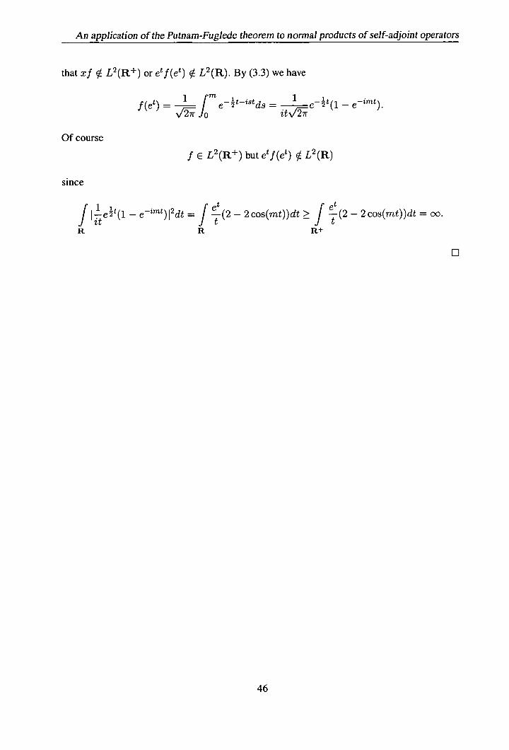
that xf V L 2 (R) or etf(et) V L 2 (R). By (3.3) we have
1 prn f( et) = J e_t_i8tds = 1 6_t(i - e_zmt)
it/
Of course
f E L(R) but etf(et) V L 2 (R
since
I I e t(1 - e_imt)I2dt = f -(2 - 2cos(mt))dt ~ f -(2 - 2cos(mt))dt = 00.
it R R
46

Chapter 4 Self-adjointness of the perturbed wave
operator on L 2 (R2 )
4.1 Introduction
There are many classes of unbounded real-valued Vs for which — L + V is self-adjoint (see,
[3], Section X.1 to Section X.6) which is very important in quantum mechanics. Many of those
results exploit the fact that — A is positive (see, e.g., [191). What we will be doing in the next
two chapters is to investigate the self-adjointness of 0 + V (there is no need to say that it is
easier to prove that something is self-adjoint than to prove that it is not). This work may not
have any direct application to another science and for the moment it is only a mathematical
curiosity.
We will also observe the difference between the wave operator and the Laplacian in the way
they behave. There is also another difference that is worth mentioning that is: the Laplacian
is a positive operator while the wave operator has no sign. In the end we will also give a
counterexample showing another difference.
In this chapter we are only interested in the case L 2 (R2 ). We want to find a class of unbounded
V: R2 - R such that D + V is self-adjoint on D(D). For V essentially bounded the result
is true either as a consequence of the Kato-Rellich perturbation theorem or as will be shown
below. We also recall that 0 + V is essentially self-adjoint on C8°(R2) (see the discussion
after Corollary 4 and Remark 11) if
/ 2 82
-
U(x, t) + V(x, t)U(x, t) = ±iaU(x, t) (ce> 0) ~jt_2 ~~X_2 )
has a unique solution in L 2 (R2 ) (that is U = 0) and eventually self-adjoint on D(D) fl D(V)
if we also prove that U + V is closed on D(E) fl D(V).
47

Self-adjointness of the perturbed wave operator on L 2 (R 2 )
4.2 First class of self-adjoint El + V
Remark 19. The natural domain of V is {f E L : Vf E L 2 }
Proposition 23. Let 0 be the wave operator on L2 (R2 ). Let V E L°°(R 2 ) be real-valued.
Then 0 + V is essentially self-adjoint on Co' (R2 ).
Proof. We shall attempt to solve the adjoint equation directly by using the Fourier transform.
We need to show that the following PDE
Ou±iau= Vu (4.1)
has a unique solution in L 2 (R2 ) that is, u = 0. Put M = llVlI. We also choose c > M.
Now take the Fourier transform in equation (4.1) and we get:
(2 + 2 ± ci)ü= t?.
Then
1I(_2 + 2 ± ai)ü11 2 ~! a ll fL I12 = IIUII2.
VIVMS
II(_2 + e2 ± ci)1iLII2 = IIvu1I2 :!~ M11u112.
Hence
0 < a11u112 M11u112 = (M - a) 11u112 > 0 u = 0.
. Remark 20. The result is true in any dimension n > 2 by the same method and for any con-
stant coefficient symmetric partial differential operator. Also, it is known that a multiplication
operator by a real-valued essentially bounded function, when added to a self-adjoint operator,
does not destroy its self-adjointness. In fact, it is an immediate consequence of the Kato-Rellich
Theorem (Theorem 19).
First recall that Li is an unbounded self-adjoint operator on D(0) = If E L 2 (R 2 ) : Of E
L 2 (R2 )} by means of the Fourier transform (c.f. Example 11).
We now we give the first class of unbounded Vs for which the operator 0 + V is self-adjoint
on D(0) but before that, we get classes of real-valued V for which92 + V is be self-adjoint
48

Self-adjointness of the perturbed wave operator on L 2 (R2 )
on 82
D(5) = { e L2 (R2 ) : E L2 (R2 )} 8 .
And then the results for 0 will follow by a change of variables.
Definition 35. Set
M'2 = {9 E L 2 (R2 ): E L 2 (R2 )}
and set M2 =
{ E L 2 (R2 ) E E L2 (R2 )}.
We also denote by p, the frnction .
Proposition 24. For all a> 0, there exists b> 0 such that
2 2
ess sup f ,(x + A, y + A)I2dA 2
a 5X
+ bIIII (4.2) x,yER
R
for all E M12
Proof. We shall first prove the proposition for CO' functions then extend the result to functions
in M12 . Let p e CO' then we have the following identity for
fp
(x, y) = J
p + (x, t) + (s, y) - (s, t) t
which is an easy consequence of the fundamental theorem of calculus. We also note that s and
t are yet to be chosen.
We have
Ix+\ py+) ço(x + A, y + A)
= J p + (x + A, t) + (s, y + A) - (s, t) t
where A is a real number.
Then
zx+.\ py+A
k(x + A, y + A) I ~ J I,I + k(x + A, t)I + k(s, y + A) I + I(s, t) I. (4.3) t
49
Self-adjointness of the perturbed wave operator on L 2 (R2 )
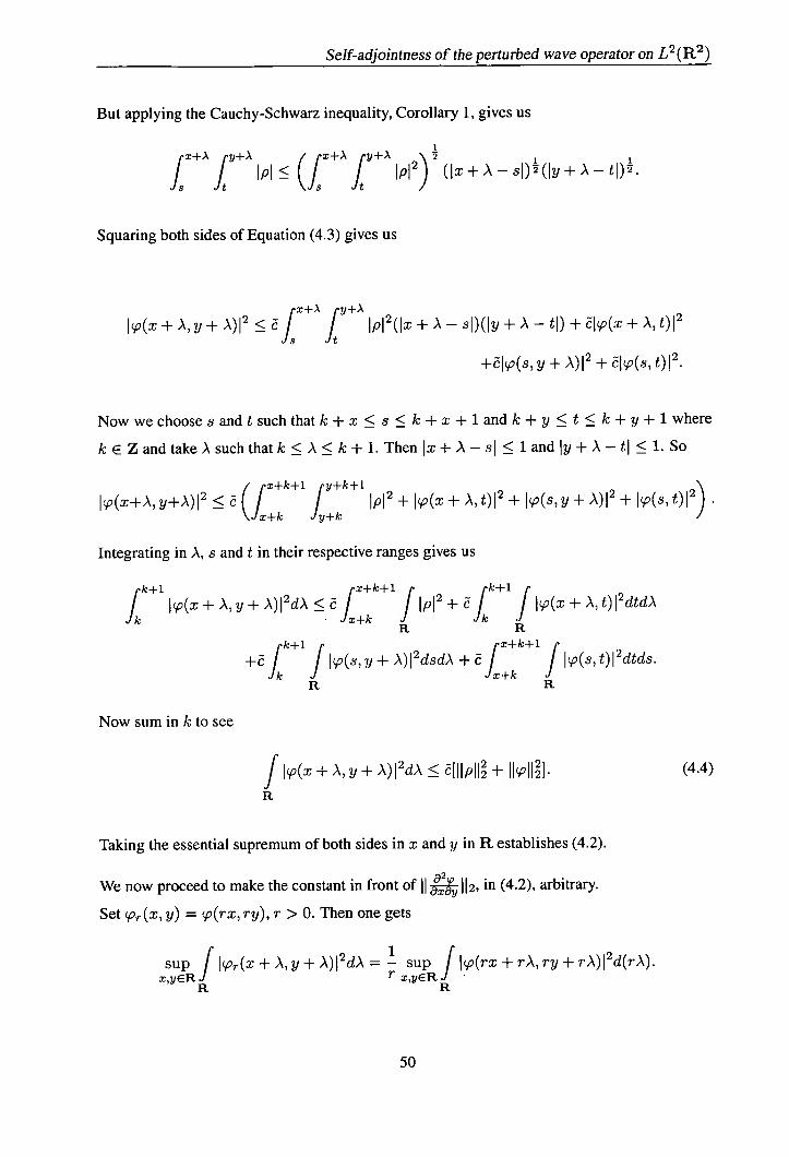
But applying the Cauchy-Schwarz inequality, Corollary 1, gives us
x+A y+A
p1 (IX+A f y+
IPI) (Ix+A—sI)(Iy+A—tI) 12
Squaring both sides of Equation (4.3) gives us
x y+) I(x + A,y + A)12 <f
+A f pI(Ix + A - sl)(ly + A - ti) + I(x + A,t)1 2
+I(s, y + A) 12 + ëI(s, t)1 2
Now we choose s and t such that k + x < s < k + x + 1 and k + y < t < k + y + 1 where
keZ and take AsuchthatkA<k+1. Then Ix+A — sl!~,1 andly+A — tIl.So
(fx+k fy+k k(x+A, y+A)12 e
x+k+1 y+k+1 p1 2 + I,(x + A, t)1 2 + I(s, y + A)1 2 + (s,t)1 2
Integrating in A, s and t in their respective ranges gives us
pk+1
fx+k
x+k+1 ç fk
k+1 (x+A,y +A)I 2dA C I II +C I l(x + A,t)I 2 dtdA J J
R R x+k+1
fk+1 j
fx +k
p
J Ico(sY+A)I2dsdA+C J (s,t)I2dtds.
R R
Now sum in k to see
(x + A, y + A)I 2dA ~ C[p + lIII1. (4.4) f
R
Taking the essential supremum of both sides in x and y in R establishes (4.2).
We now proceed to make the constant in front of II 112, in (4.2), arbitrary.
Set cor (x,y) = ço(rx,ry), r > 0. Then one gets
Sup f r(x + A, y + A)I 2 dA = sup II(rx + rA, ry + rA)1 2 d(rA). x,yER r x,yER
R R
50
Self-adjointness of the perturbed wave operator on L 2 (R 2
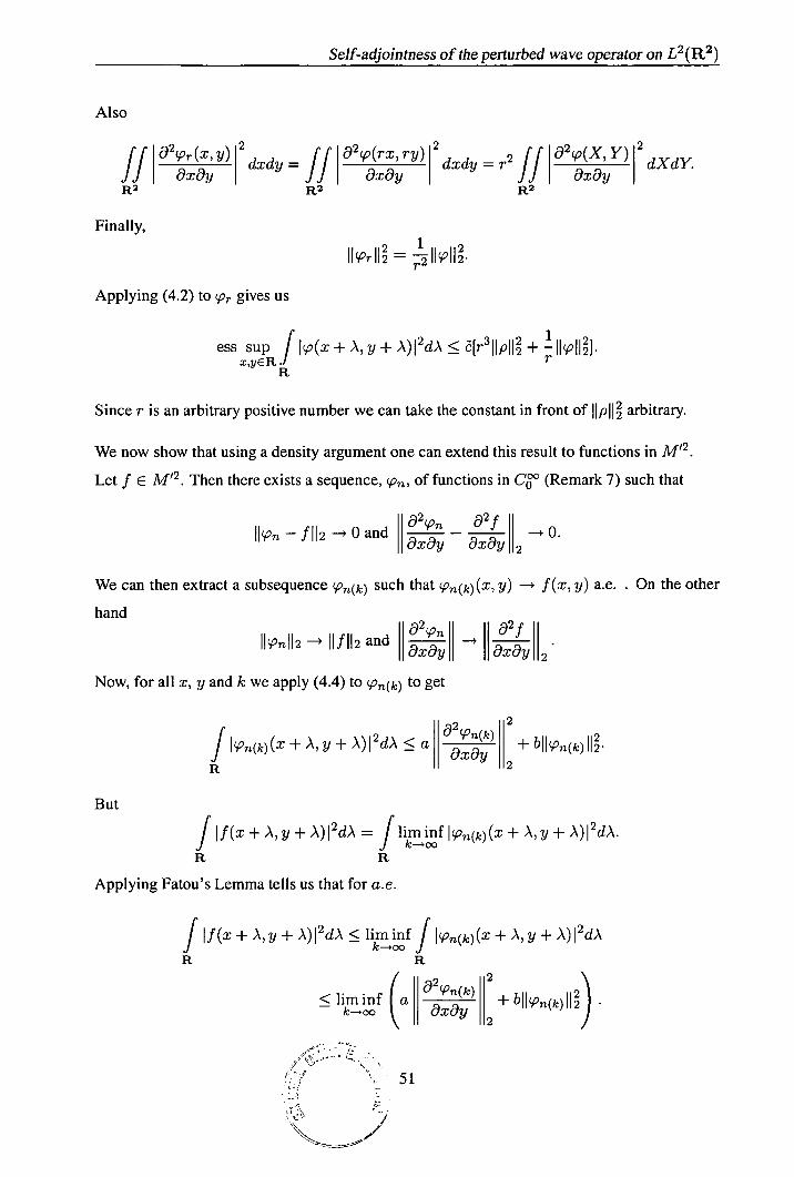
Also
If ö2cor(x, 2 dxdy ff 82 ço(rx, ry) 2 02 (X, Y) 2 axl9y = ôxôy
dxdy = r2 ff R2 R2 R2
Finally,
Ik2rII = II'pI
Applying (4.2) to W, gives us
ess sup f (x + A, y + A) 12 e[r3 IIpII + IIII]. x,yER r
R
Since r is an arbitrary positive number we can take the constant in front ofarbitrary.
We now show that using a density argument one can extend this result to functions in M'2
Let f e M'2 . Then there exists a sequence, ço, of functions in Co' (Remark 7) such that
ii - I IIn - fII -* 0 and
82 0 21I - 0.
Moo 8x0yI 2
We can then extract a subsequence n(k) such that co(k)(x, y) -p f(x, y) a.e. . On the other
hand
fl 92fPII2—IIfII2ad oxoy aXay 2
Now, for all x, y and k we apply (4.4) to to get
2 lIo2() 2
<all +bIkOfl(k) 11 2 . f + A, y + A)I dA - 1
R
But
f If(x+ A,y + A)I 2 dA = f 1iminfI fl(k) (x + A,y+ k-400
R R
Applying Fatou's Lemma tells us that for a.e.
If(x + A,y + A)I 2dA liminff fl(k)(x + A, y + A)I 2dA f k—oo R R
<liminf (a +blIfl(k)
82 c 2
- koo OxOy II).
51

Self-adjointness of the perturbed wave operator on L 2 (R2 )
Taking the essential supremum in x and y establishes (4.2) for functions in M12. Li
We now give the first class of unbounded Vs.
Theorem 27. Let LI be the wave operator in L 2 (R2 ). Suppose V is real-valued such that
11V11 2 = f suplV(ij, e)I 2d <oo. Then Li + V is self-adjoint on V(E) = M 2 C L 2 (R2 ). R 7ER
Proof Set
(x,y)(x+y x—y\ = 2 ' 2
)/)(77i)
(then = 02 82
where Li is -
We have
IIVII = ffIv(me(m)I 2dde. R2
We also have
f V (71 , e)(m )I2d sup I V(, e)12 J , ) 12 d77. ijER
R R
But
f I(m)Idi = f (i+-
e)12 d77= f IA +e,A - )I2dA.
Hence
IIVIl f supIVI2 fI +,A)I 2dA d. ijER
R R
Therefore
iiVii ~ I( + )I2 IV( )I 2 sup dA sup d ER
f ijER Lf
Now by Proposition 24 one obtains
/ 2
IIVII Isp IV(m)I 2 dR
a + bIIII)tER
Thus
IIVII ~ o LfV121
(aIIDII + bIIII). (4.5) 77ER
By Equation (4.5) we can see that D(V) C D(D). Hence V is Li-bounded and since we can
52
Self-adjointness of the perturbed wave operator on L 2 (R 2 )
make the constant a in front of 1100 112 as small as we like (Proposition 24), we conclude by the
Kato-Rellich theorem (Theorem 19) that 0 + V is self-adjoint on D(0). 0
Remark 21. In Chapter five we will give another method to get exactly the same norm of V by
using Fourier transforms. We do not want to give this method here since it also works in higher
dimensions so we prefer to leave it until then.
4.3 M12 and the space BMO
Now we prove an important estimate that will allow us to say that 0 + V is self-adjoint for any
real-valued V E L 2 (R 2 ),Ve > 0.
Before that we show that M12 C BMO(R 2 ). Then it will follow by the sharp maximal
theorem (Theorem 7) that M12 C L", 2 < p < 00. We will then deduce that M 2 C LJ'(R2 );
2 < p < oo. We first have
Theorem 28. Let E M'. Then E BMO(R 2 ) and
II II IkPIIBMO(R2) <a 0x I2
+ bIIII2 (4.6)
where a and b are two constants.
Theorem 28 will only be proved for C6°-functions (to get the estimate (4.6) for functions in
M12 we use the usual density argument c.f. the proof of Proposition 24). The following lemma
will be needed in the proof of Theorem 28.
Lemma 10. Fix y' E R and put fi (x) = p(x, Yi) where o e C°. Then f' E BMO(R) with
uniform BMO bound, i.e.,
IIf1IIBMo(R)a "0 II + bII , Il2 axay 2
Also fir x 1 then y -f gi(y) = ço(x i , y) is in BMO(R).
Proof. We have to prove M1 f1 Jfi(x) - iIdx < c where c does not depend on y, and where
= -} T f1 f i (x)dx. Then we have
fV
yi (Ii - H(X) = p(x, z)dz where 1(x) = (x, y)
53

Self-adjointness of the perturbed wave operator on L 2 (R 2 )
and where we have the freedom to choose the y that is convenient for us. Then we have
fyi
1(1' - f)'II = [I(fi - f)'(x)I 2dx = [i p(x, z)dzl 2 dx. JR JR
Thus
(li - f)'II ~ (i - <00 with the assumption y < y.
So (fl - f)' E L(R) hence (fi
- 1)' e L' (R) and so f - f is absolutely continuous on 10
every compact set of R hence continuous. So the average fi - f is (fl - f)(c) where c E I
and such a c exists by the intermediate value theorem. So
(fi — MX) — fi — f= (fi — MX) — (fi — MO.
Since fi —f is absolutely continuous on I, it is differentiable almost everywhere, (fl —f)' E L'
and
(f' - MX) - (fi - f)(c) =
f - f)'(t)dt
and then
(li - MX) - U1 - f)(c)I f (fl - f)'(t)Idt < (x - c) 11 (fl - f)'112.
Then
(fi - f)(x) - (1' - f)(c)I <(b - a) II(fi - f)'112 = III II(fi - f)'112
and hence
fI(fi - f)(x) — (fi — f)(c)Idx < IIIII(fi - f)'112.
But we have I(fi - f) ' 112 (yi - Y) '! IIPI12- So in order to find a uniform bound for 1 1fi -
Ill BMO for this particular I it suffices to take y such that (y, - y) _Lr and in such case we 117
will have:
jj (f' - f)(x) - (1' - f)Idx IItII.
But our interest is in the function Ii itself not in fi - f so from f,(x) - fi(x) - f(x) -
Ti + 7+ f —7 (since f --g = f - ) we can find a BMO bound for Ii for this particular
I if we come to show that f is BMO. We have
1 I 1 1 if(t)Idt)dx jj If - lids jj j, if(x)idx + -j J(j
54
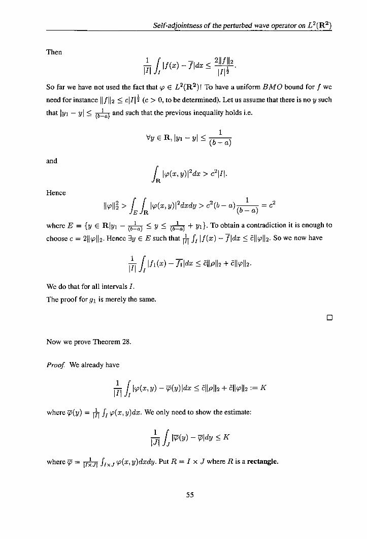
Self-adjointness of the perturbed wave operator on L 2 (R 2 )
Then
If (x) - lldx < 2 111 II2 - lIl
So far we have not used the fact that E L 2 (R 2 )! To have a uniform BMO bound for I we
need for instance 111112 <clIl 2 (c> 0, to be determined). Let us assume that there is no y such
that Iyi - I < 1 and such that the previous inequality holds i.e.
Vy E R, Iyi - I < 1
(b — a)
and
JR I(x, y)I2dx> C2
Hence
lIIl> fE / (x,y)I2dxdy > c(b— a)_1
= c2 JR (b — a)
where E = { y E RIyi - y + y}. To obtain a contradiction it is enough to
choose c = 2IIII2. Hence 3y E E such that .11 11(x) - lIdx < cII'II2. So we now have
j J Ifi(x) - iIdx —< ö11t112 + clIII2.
We do that for all intervals I.
The proof for gj is merely the same.
Now we prove Theorem 28.
Proof. We already have
JJ i: I(x, y) - (y) Idx < eIIplI2 + C1k2112 := K
where (y) = M 1 f1 x, y)dx. We only need to show the estimate:
F ' ( I() - Idy < K
where iT = Txl—jT (x, y)dxdy. Put R = I x J where R is a rectangle.
55
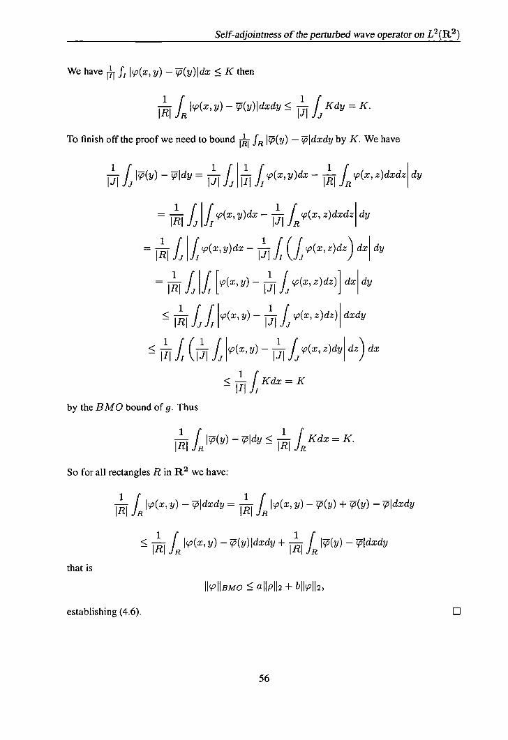
Self-adjoin tness of the perturbed wave operator on L 2 (R2 )
We have J'1 k'(x, i') - (y)Idx < K then
F ' f I W (x, y) — iT(y) I dxdy :5 j 1jj fKclY=I<
To finish off the proof we need to bound -k fR I() - TJdxdy by K. We have
f J~P(y) — Idy= j f jj f ço(x,y)dx — f cO(x, z)dxdz dy
1 fI[d 1 fR RI jIi JI
1 (jRI iii IJI ) I
= j-ff PX,Y)_ jjjc(xz)dz)] dxdy
< 1Ii 1I - I
- IRI fi
-iii1 f (jH(x,y)_ f (x,z)dydz ) dx
< j fKdx = K
by the BMO bound of g. Thus
FR I L I() - Idy I Kdx = K. IRI J
So for all rectangles R in R2 we have:
-j f (x, y) - Idxdy = -1 j f k(x, y) - (y) + (y) - Idxdy
1' I'
-J Ic'(x,y) —(y)Idxdy+ 1
-J I() — Idxdy IRI R IRI R
that is
Ik°IIBMO : ~ aIIpII2 + bII'II2,
establishing (4.6). 701
56
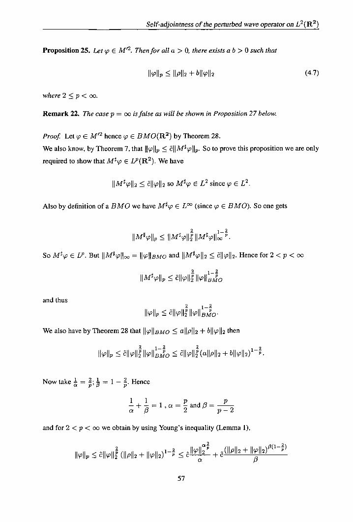
Self-adjointness of the perturbed wave operator on L 2 (R2 )
Proposition 25. Let W E M12 . Then for all a > 0, there exists a b > 0 such that
koII :5 11P112 + bIIwII2 (4.7)
where 2 < p < 00.
Remark 22. The case p = oo is false as will be shown in Proposition 27 below.
Proof. Let V E M12 hence 'P E BMO(R 2 ) by Theorem 28.
We also know, by Theorem 7, that II'PIIp !~ E 11MOW 11 p . So to prove this proposition we are only
required to show that M O W E LP (R2 ). We have
IIM'II2 :5 Z 11W112 so M O W E L 2 since W E L.
Also by definition of a BMO we have M O W E L (since W e BMO). So one gets
IIMcoIIp :!~ IIMpII 2 00 IIMI
So Mt ço E L'3 . But IIMIl = II'PIIBM0 and IIMII2 :!~ all W I12. Hence for 2 <p < 00
IIMcoIIp :!~ EIIVI12P Ik°IIBMQ
and thus 1-
'P c p_ 'P2p IIVII BMPO I
We also have by Theorem 28 that II'PIIBM0 :~ ap2 + bIJ'P112 then
IkII < CII'P112 lI'PII o < oIIII(aIIpII2 +
. Now take 1 2 = , 1 -
_ 1 - . Hence
and for 2 <p < oo we obtain by using Young's inequality (Lemma 1),
3(1-)
cIIII (11P112 + II'P112) + M2 + I'P112) II'PIIp ~
a 13
57
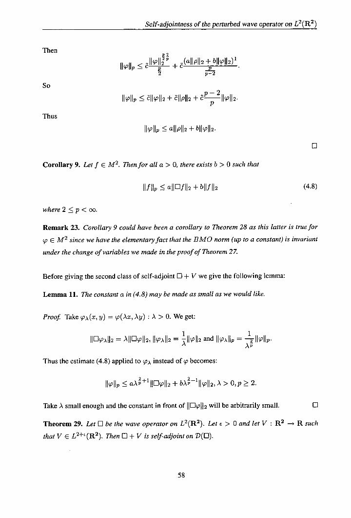
Self-adjointness of the perturbed wave operator on L2 (R 2)
Then 2 p
IIWIIP ii 11 (aIIpII2 + bIIcII2) 1
_2. 2 p-2
So
Il9iI !~ C1k0112 + E IIPI12 +
Thus
III a11p112 + bIIII2.
07
Corollary 9. Let f e M 2 . Then for all a> 0, there exists b> 0 such that
Ill lip <aJLJf 112 + bIll 112 (4.8)
where 2 < p < 00.
Remark 23. Corollary 9 could have been a corollary to Theorem 28 as this latter is true for
E M 2 since we have the elementary fact that the BMO norm (up to a constant) is invariant
under the change of variables we made in the proof of Theorem 27
Before giving the second class of self-adjoint D + V we give the following lemma:
Lemma 11. The constant a in (4.8) may be made as small as we would like.
Proof Take A(x,y) = çoAx,Ay) : A >0. We get:
1 1 II0oA1I2 = AIILipII2, II'A112 = ikII2 and IIAIIp = --II'II.
Thus the estimate (4.8) applied to ço instead of ço becomes:
JIVIl p <aAp + bA'IIII 2 , A > O,p ~: 2.
Take A small enough and the constant in front of IILiI12 will be arbitrarily small. 0
Theorem 29. Let 0 be the wave operator on L2 (R 2 ). Let e > 0 and let V : R2 -' R such
that V E L 2 (R2 ). Then 0 + V is self-adjointon V(D).
58

Self-adjointness of the perturbed wave operator on L 2 (R2 )
Proof We have by Corollary 9,
<aflD + bIII12, for 2 < p < 00.
Then by the generalized Holder's inequality:
Il'II2 :5 flVlI q llll p :~ aIVIJ q ilElço112 + biIVil q ll2Il 2 , for 1 =
1 - + - or p q
q = (this actually means that q -* 2 as p -* oo).
Since the constant in front of may be made arbitrarily small so that we have allVlI q < 1
we conclude by the Kato-Rellich perturbation theorem that 0 + V is self-adjoint on D(El) =
M 2 . 0
Remark 24. Adding a bounded multiplication operator by a real-valued function does not
destroy the self-adjointness and we have:
Proposition 26. Let V E L 2 (R2 ) + L°°(R2 ) be a real valued function, €> 0. Then El + V
is self-adjoint on D(D).
Proof. We have
llyllp <aE + bllll2.
Put V = V1 + V2 where V1 e V2 E L°°. Then llV,112 = lI(Vi + V2)l12 and by the
generalized Holder's inequality (Proposition 1)
llVco112 :~ llV1ll2+€Il11 + llV2I111'l12 all V1 lI2+€llDPll2 + (llV2I1 + b)ll112.
Since we can take a as small as we like, 0 + V is self-adjoint on M2 by the Kato-Rellich
Theorem. 0
Example 17. Let s > 1. Take V(x, t) = 1 1 Choose c > 0 such that 2+ < 2. Then
7X2 +t2) S
V E L 2 + L°° and hence 0 + 1 is self-adjoint on M 2 . (x2 +t2 ) 2
4.4 Counterexamples
It was mentioned in Remark 22 that a function in M 12 needed not be in L°°. So we have
59

Self-adjointness of the perturbed wave operator on L 2 (R2 )
Proposition 27. Let L 2 (R2 ) such that a2 2 ff Y E L(R 2 ). Then w need not be essentially
bounded on R2 .
We give two methods of how to do this. First we give an explicit counterexample that we
construct in the following proof:
Proof. We are going to build up the counterexample by using a linear interpolation. We define
(x, y) '-p (x, y) on R x (yn, yn+i] by
(x, ) =
Yn+i 1 - Yn [(y - y)f+1(x) - (y - y1)f(x)] where f. (x) = (x, y)
and the f and yr, are to be defined below.
Observe that p is only defined for y> y := 0. At the end of this proof we will extend it to the
case y < 0 by a symmetry.
Hence on R x (0, oc) we have
00
koII= ff Iw(x,y)I2dxdy=> ff I(x,y)I2dxdy
Rx(O,00) 1 Rx(y,yi]
In order to have in L 2 (R x (0, oo)), it is sufficient to have
00
(y.+1 - ym)(IIfII + IIfm+iII) <Oo.
We also have 1
= Yn+1 - (f 1 (x) - f(x)).
Yn
In order to have 82-
in L 2 (R x (0, oo)), it is sufficient to have
00 1
IIP' flhI
2 2 <00 where '(x) = fm+i(x) - f(x). Yn+1 - Yn
00
We are going to to define fn by first constructing then putting fn (x) = - Vk(x).
We also want fn L°°(R) so that ço L°°(R 2 )
zo

Self-adjointness of the perturbed wave operator on L 2 (R2 )
Take
n — 1
{
— - e--x OrL (x)
0
if —eTh<x<O,
if 0<x<e,
if lxi > e.
Hence il/ and li'nli - We also have
00 00 _! 00 X -z
2 e 1 100
— e 2
2=a - J — dx< — e 2 dx-----ifll2 ~ lkbkii Ti — k=n k=n
Now if we choose Yn+1 - = e72 then the series
00 1
002 1 e 00
E iinil2= X -
2 obviously converges. n+
/ 2
And so does the series
00 00 00 e' 1 2 i 2 ____ X 21 'i2 1 1
Now the W defined on R x (y, Yn+i) is given by
00 00
(x ) y) = e [(Y_Yn (—n+l
k(x)) - (yyn+1) (_k(x))].
This p is actually defined only for x E R and y > 0. To extend it to the case y < 0 we define
for x E R and Yn+1 <y < as follows:
1 (x, y) = [(y - ym )fm+i (x)
— (y - Yn+1 — Yn
This p is clearly in M'2 . Now we need to show that p is not in L°°(R 2 ). Let x > 0 and
X < e_c then In x < —kor1n > k. So
in J k [in 1
[in j 1 f(x)=—x -+ .(_x2+1)
61
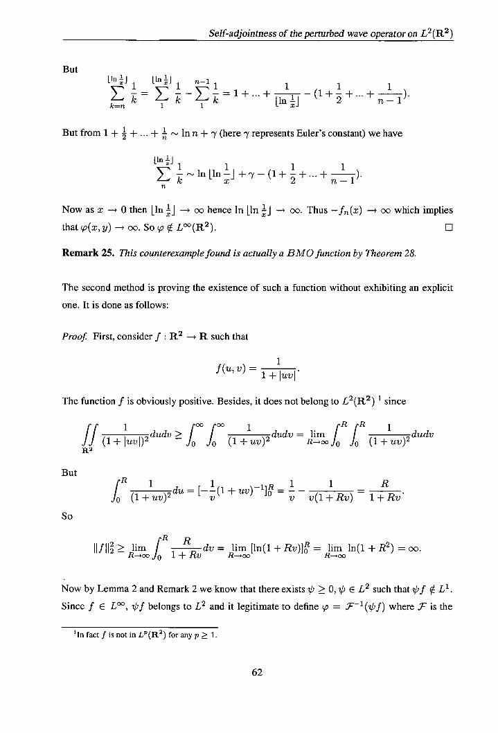
Self-adjointness of the perturbed wave operator on L 2 (R2 )
But 1n J 1n
1 1 1 i = i k= 1+...+ Li1j_ (1+_ 2 +... n— + 1 k=n 1 1
But from 1 +.1 + ... + ".' in n + -y (here y represents Euler's constant) we have
1n 1 j
1n [In .j+y—(1+ +... + 1
n- n
Now as x -* 0 then [in j -* 00 hence in [in j -* 00. Thus —f , (x) -p 00 which implies
that (x, y) -* 00. So L°°(R 2 ). L]
Remark 25. This counterexample found is actually a BMO function by Theorem 28.
The second method is proving the existence of such a function without exhibiting an explicit
one. It is done as follows:
Proof. First, consider f : R2 -* R such that
1 f(u,v) =
1 + Iuv
The function f is obviously positive. Besides, it does not belong to L 2 (R 2 ) since
11 dndv = urn
fo
R 1R
ff(l+IuvI)2dv ~ L L (1+uv)2 Roo Jo (l+uv)2dudv R2
But pR 1 1
du=[--(1+ —1R
Jo (1+uv)2 UV) ]
1 1 R V v(1+Rv) 1+Rv
So
çR 11f11 2 > urn / R dv = urn [ln(1 + Rv)] = urn in(1 + R 2 ) = 00. R—oo .10 1 + Rv R—oo
Now by Lemma 2 and Remark 2 we know that there exists 0 ~! 0, O E L 2 such that Of L 1 .
Since f E L°°, Of belongs to L 2 and it legitimate to define ..T' (0f) where ..F is the
'In fact! is not in L' (R') for any p > 1.
62

Self-adjointness of the perturbed wave operator on L 2 (R2 )
L 2 -Fourier transform. By the Plancherel theorem V is in L 2 . Also
( axay) a
= UVJC"W = uv(u,v)f(u,v).
uv uv - ______ Since (u, v) i-p 1+IuvI L°°(R 2 ) and since E L 2 (R 2 ) it follows that 1+IuvI E L 2 (R 2 )
and hence, as a consequence of the Plancherel theorem, one gets that ffx- y E L 2 (R2 ).
Before carrying on the proof we give the following lemma:
Lemma 12. Let L 2 (R"). If ç V L'(R') with 0 > 0, then W V L°°(R)
Proof Let W E L 2 (R"). Suppose W e L(R). Take
fp,m(X) = P * ',bp)gm(x)
where Op is a smoothing function like the one defined in Theorem 2 that satisfies Ik1'pII 1
(take 1 = E). We assume that 9m > 0 and it is a C°-function. We finally assume that 9m tends
to one pointwise. Then we have fp,m e L' (Rn) and fp,m > 0.
We now apply Proposition 3 to have
IIfp,7n111 = lIfp,mIIoo
Applying Young's inequality for convolution, taking ç(x) = (—x) and since ç' = gives us
-. II (P * çbp)gmIIi
=
1
(2ir) II(') * g. 11.
1
(2ir) II(Pp II oo Il gm II 1 <00.
Or
11 P * bp)gmi (2r) 121
So as p tends to infinity we obtain
IN * 1p)gmi - IIc'gmII1.
In the end one has
f (x)gm(x)dx = 9gmII1 (27r) 121
IkoPIIoo (2ir)
Rn
63
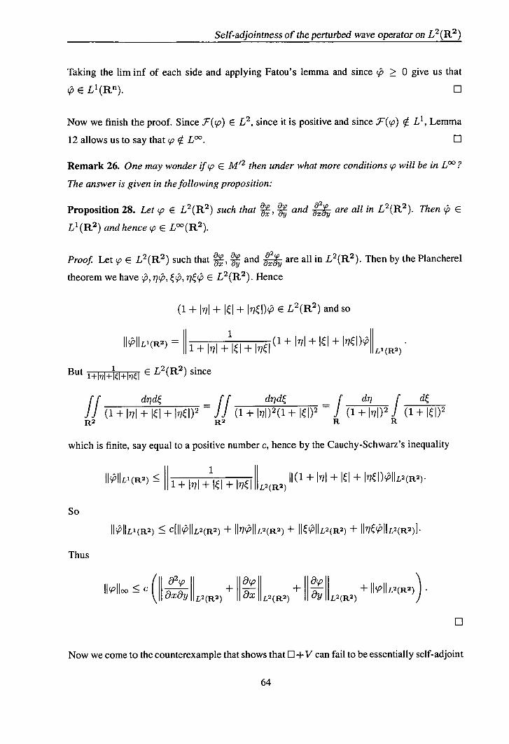
Self-adjointness of the perturbed wave operator on L 2 (R2 )
Taking the urn inf of each side and applying Fatou's lemma and since 0 give us that
çEL'(R). 0
Now we finish the proof. Since F() e L 2 , since it is positive and since .F() V L', Lemma
12 allows us to say that ço L°°
U
Remark 26. One may wonder if ço E M 12 then under what more conditions will be in L' ?
The answer is given in the following proposition:
Proposition 28. Let L 2 (R2 ) such that , and are all in L2 (R 2 ). Then ç' E
L'(R 2 ) and hence V E L oo (R 2 ).
Proof. Let E L 2 (R2 ) such that and are all in L 2 (R 2 ). Then by the Plancherel
theorem we have 0 , 770, , rç e L 2 (R 2 ). Hence
(1 + 1,qj + + 'qj)c' E L 2 (R 2 ) and so
1 II II
(1 + ijl + II + II)' IIIIL1(R2) = 1+ + ii + 174 1IL 1 (R2 )
But 1 E L 2 (R2 ) since
if d7j< - ff d77d f dij f
(1+ II + iei + II)2 - ( 1+ II) 2 (1 + II) 2 = ( 1+ I1) 2 1 (1+ II) 2 R 2 R2 R R
which is finite, say equal to a positive number c, hence by the Cauchy-Schwarz's inequality
II
L2(R2) 10IILl(R2) < 1+I
II 11( 1 + IiI + II + II)cIIL 2 (R 2 ).
77I+l
1
)I II 1 I+I
So
I10IILl(R2) < c[IIcIIL2 (R 2 ) + II77011L2(R 2 ) + IIe0IIL2 (R 2 ) + II 7)0IIL2(R2)1.
Thus
IIPlIo -
( a
Y
x IIlI
19Y+ II
210 ( ) ).
Now we come to the counterexample that shows that LI + V can fail to be essentially self-adjoint
64

Self-adjointness of the perturbed wave operator on L 2 (R2 )
if V E L(R2) and we have:
Proposition 29. Let LI be the wave operator defined on L 2 (R2 ). Then there exists a real-valued
V. V E L2 (R2 ) such that LI + V is not essentially self-adjoint on C.
Proof. Basically we want to show that the following PDE has a non-zero solution in L 2 (R2 )
for some V E L(R 2 ):
782 82 \ - -) (x, t) + V(x, t)ço(x, t) = 2iço(x, t).
By Example 16 we can say that the following ODE:
d2
——.f (x) - x 4 f(x) = if (x) (4.9)
has a non-zero solution in L 2 (R). And we can say the same thing about
d —ig(t). (4.10) 2
—-g(t) - t 4g(t) =
Now by multiplying (4.9) by g(t) and (4.10) by —f(x) we obtain:
d2
—g(t)—f(x) - x 4 f(x)g(t) = if (4.11)
and
f(x)j d2
g(t) + t4 f(x)g(t) = if(x)g(t). (4.12)
Now by adding up (4.11) and (4.12) we get
/02 02
- -) f(x)g(t) + (t 4 - x 4)f(x)g(t) = 2if(x)g(t). (4.13)
Take (x, t) = f(x)g(t). Since f, g are both in L 2 (R) then cc' will be in L 2 (R2 ) and (4.13)
X 4 2 will have a non-zero solution in L 2 (R2 ) with V(x, t) = t4 - E L(R 2 ).
Thus- + t4 - x4 is not essentially self-adjoint on V(D). Li

Self-adjointness of the perturbed wave operator on L 2 (R 2 )
4.5 Open problems
Let V be a real-valued function such that V E L 2 (R2 ). The question is: is 0+ V essentially
self-adjoint on C?
This is more likely to be wrong since we did not obtain (for p = oo)
II! lip < ailEf 112 + bllf 112,
which would have allowed us to conclude that 0 + V is self-adjoint for V real-valued and in
L 2 (R2 ) or essentially self-adjoint on Co'.
It is worth mentioning that - + V is self-adjoint on D(—/) C L 2 (R 3 ) (c.f. Example 14)
and the proof of that exploits
f1100 <all - f112 + 11f112
(Theorem 6) and the Kato-Rellich theorem.
So one may even conjecture that if for some self-adjoint partial differential operator P one does
not have an inequality of the type
11100 <alIPfI12 + blIf 112,
then there exists a real-valued V, V E L 2 (R'), n > 1 for which P + V is not essentially
self-adjoint on C000 .
Now we go back to our open problem. One way of showing that 0 + V is not self-adjoint (or
at least not essentially self-adjoint on C°(R 2 )) is to construct a V which is in L 2 (R 2 ) and not
in L(R 2 ) for s > 2 and show that
( - f(x, t) + V(x, t))f(x, t) = ±if(x,
has a non-zero solution which belongs to L 2 (R2 )
If V > 0 is real-valued and in L2 C,
is Li + V essentially self-adjoint on C000 ?
If V > 0 we cannot use the same method as the proof of Proposition 29 since it is known (see

Self-adjointness of the perturbed wave operator on L 2 (R 2 )
r2 d2 [191) that for V > 0 and V '1oc' - + V is essentially self-adjoint on C°.
This question too has probably a negative answer. A possible counterexample would be V(x, t)
It4 - X41 but one has to investigate that.
67

Chapter 5 Self-adjointness of the perturbed wave
operator on n > 3
5.1 Introduction
In this chapter we investigate the self-adjointness of E + V for n > 3 and V real-valued and
unbounded. The wave operator worsens in higher dimensions and as a result we will have
smaller classes of Vs and hence more open problems.
5.2 A class of self-adjoint LI + Von L 2 (Rrt), n > 3
Definition 36. We set
= {u E L 2 (Rh1) : Lu, as a distribution, is an L 2 (R n1 )function I.
We first start by the case n = 3. Before we give the first proposition let us discuss the following
Cauchy problem:
(I) f Utt - - u = f(x ) Y, 0, (x ) y, t) E R2 x
u(x,y,O) = (x,y);u t (x,y,O) = b(x,y).
Now let us take the Fourier transform of (I) in the (x, y)-plane only. We get:
(I) I (77
( 77, =
(I) is a second order ODE in t with constant coefficient (with respect to t) and it has the

Self-adjoin tness of the perturbed wave operator on L 2 (Re), n > 3
following solution in the homogeneous case:
= (m ) COS (t + + sin(t -+V ). V772 + 2
Then by using the Duhamel's principle the general solution of (I) will then be:
= ( 77, ) COS (ti12 + 2) + V772 +2 sin(t + 2)
(5.1) / 2 +2(t - s)d + / f(is,,$)
sin
Jo
The previous holds for t > 0. Also for t > 0 (I) becomes, after setting u(x, y, t) = u(x, y, —t),
(I) f (x7y,t)ER2xR
u(x,y,O) = (x,y);üt(x,y,O) = —'L(x,y).
Now we "fourier" everything in the (x, y)-plane to obtain
I tt + (2 + (I) (m, 0) = ,O)
which has the following solution:
= t) = cos(t2) - sin(t 2) V77 2 -+ V
(5.2)
f-t v' 2 + 2(—t - s)
d+ +
d,9 e2
and this holds fort > 0. After adding up (5.1) and (5.2) one gets (still fort > 0)
= 2(ij,)cos(tj2 + 2 ) + [ s) sin
+(t - s) ds
+f—ts)
sin ii2 + 2 (—t - s) ii
(5.3)
ds — (— t)
Now Equation (5.3) is unchanged if t is replaced by —t. So (5.3) holds for all t E R.
Now we can change our Cauchy problem by introducing different initial conditions mainly for
MIG

Self-adjointriess of the perturbed wave operator on L 2 (Rr), n > 3
the t variable i.e. instead of working on the intervals (0, t) and (—t, 0) we will be working on
(, t) and (a, ) where a is any real number that will be chosen freely (observe that if we
set a = —t then we go back to the initial problem).
Now given u E CO' we can regard u as a solution to the Cauchy problem with u E CO' where
f = Eu, u(x, y, 0) = V (x, y) and ut(X, y, 0) = 'iI(x, y). Then ( 5.3) will be:
t+a ü(i,t) = 2 )cos [v2 +2 (t a)] —,,a)+
(5.4)
ft
it +f(, , s)Sfl + 2(t -
s) ds + f J(, , s) sin 7 2 + e2(a - s)dS
2
Proposition 30. For all a> 0, there exists b> 0 such that
ess sup IIu(., ., 0 11L 2 (R2 ) aIlE1uIIL2(Ra) + bIIuIIL2(Ra) teR
for all u E M3 .
Proof. We shall prove the proposition for functions in C3° first then the result follows for
functions in M3 since C00° is dense in M3 in the graph norm of Li (c.f. Remark 7 in Chapterl).
We choose a such that It - at < 1 and one then obtains:
t + a + oft If(m , s)Ids + ëf IJ(ii, , s)Ids + I(j, , a)I. I'(i,t)I2Iu(me, 2 )I 2 2
(5.5)
where we have used the fact that I < 1. Using Cauchy-Schwarz inequality shows that
1
+ (f If
t + a + (ft If(' , s)I2ds)
2
2 2 2
+OIü(ii, C a) I.
Now square the previous inequality to get
t + a 2 +
lt+Qt if (77, s)I 2ds + of I f (77,
, 8)I2ds OIu(me, 2 2 2 (5.6)
+OIü(i, , a).
70

Self-adjoin tness of the perturbed wave operator on L 2 (Rn), n > 3
Then integrate (5.6) with respect to 71 and in R2 to obtain
Itt+affIi(me,t)I 2 d?id ~ ffiU 2 )I2 ff Ij(me,$)l2didds+
R2 R2 R2 2
iff If (,q, , s)I2diideds + ff ü(i a)l2diid.
L± R2
2 R2
(5.7)
And hence
u(m , t) 2djd Ii(m
t a) 2dde + lf(m , s)
LIL
LI Iu(m , a) I 2 did.
Now integrate everything with respect to a in the segment It - a 1 i.e. t - 1 < a < t + 1
to get:
i
t+1 t+1 t+ ffIu(m,t)I 2ddda ~ oL_ ff ium 2)I2d1deda
R2 R2
t+1 t+1
+oj_1 N lf(ri,,$)I2diiddsc1a+ f if R3 R2
Hence
LI Iu(m.,t)I 2did :5 oJ I(m, t±a)I2d,dda
+aN If(m', s)l 2diidds + E N
If, (m e, a)I2dijdda.
R3 R3
Thus by the Plancherel theorem one has:
t) 11 2 2 2 L2(R2) < alIDuIIL2(R3) + bIIuII2(R3). (5.8)
71

Self-adjoin tness of the perturbed wave operator on L 2 (R"), n > 3
Taking square roots of both sides then the essential supremum in t over R:
ess sup IIu(., ., t)11L2(R2) < aIlDuIIL 2 (R3 ) + blIuIIL2(R3). (5.9) tER
The result for functions in M 3 follows by the density of CO' in M 3 . Cl
Before giving the main theorem here, we first have the following proposition:
Proposition 31. The constant a in (5.9) can be made as small as we want.
Proof Take Ur(X,y,t) = u(rx, ry, rt), r >0. Then
Hur t) 1IL2(R2) = ff U(X y, t)I2dxdy = ff Iu(rx, ry, rt)I 2 dxdy
R2 R2 ft 1
= Jj —u(rx,ry,rt)I2d(rx)d(ry).
R2
which implies that: 1
1r(., ., t) IIL2(R2) = - Ilttr(.) ., rt) I1L 2 (R 2 ). r
We also have:
UrlI 2 (R3 ) Niur(X,Y,t)I2dxdydt = N Iu(rx,ry,rt)I2dxdydt
R3
= N Iu(rx, ry, rt) 2 d(rx)d(ry)d(rt).
that is 1
U7- IIL 2 (R3 ) = 3 I1LIIL2(R3). r2
Finally
IIThsrII2(R3) N =ILItt r (x, y, t)I2dxdydt = N r4 10u(rx, ry, rt)I 2 dxdydt
R3 R3
= fff rIDu(rx, ry, rt) 1 2 d(rx)d(ry)d(rt).
Hence
IIt1rIIL2(R3) = FIIU1IL2(R3).
72
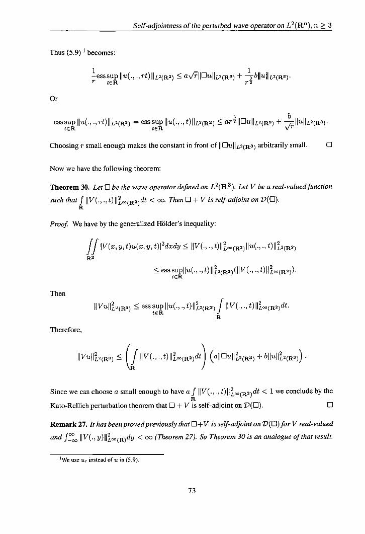
Self-adjoin tness of the perturbed wave operator on L 2 (R"), n > 3
Thus (5.9) ' becomes:
i IIuIIL2(R3) +ess sup Iu(, ., rt) 11L2(R2) <a\ bIIUIIL2 (R3 ).
Or
b ess sup IIu(., ., rt)11L2(R2) = ess sup IIu(., ., 011L2(R2) ar2 IIOUIIL 2 (R3 ) + — IIuIIL 2 (R3).
teR tER
Choosing r small enough makes the constant in front of IIDuIIL2(a3) arbitrarily small. Li
Now we have the following theorem:
Theorem 30. Let 0 be the wave operator defined on L 2 (W). Let V be a real -valued function
such that IIV(., ., t)lI(R2)dt < oo. Then Li + V is self-adjoint on D(C).
Proof. We have by the generalized Holder's inequality:
ff V(x, y, t)u(x, y, t) I 2dxdy IIV(., ., t) IIL(R2) IIu(., ., t) II2(R2)
R2
< ess sup Iu(., ., t) IIL2(R2)(IIV(., ., t) IILOO(R2)). teR
Then
IIVulI2(Rs) ~ ess sup IIu(., .,t)II2(Rz) f IIV(•, ., t)II(R2)dt. tER
R
Therefore,
IVuII2(Ra) Lf IIV(., ., t) II(R2)dt) (allEuII 2 L2(R3) + bIIuJI2(R3)).
Since we can choose a small enough to have a IIV(., ., t)II(R2)dt < 1 we conclude by the
Kato-Rellich perturbation theorem that Li + V is self-adjoint on D(0). Li
Remark 27. It has been proved previously that Li + V is self-adjoint on D(D) for V real-valued
and fff 11 V(., y)If(R)dy <00 (Theorem 27). So Theorem 30 is an analogue of that result.
'We use Ur instead of in (5.9).
73

Self-adjointness of the perturbed wave operator on L 2 (R"), ii > 3
Besides one has another method to find that norm of V as the method in this work is applicable
to the two-dimensional case and even to any dimension and we have:
Proposition 32. For all a> 0, there exists b> 0 such that
ess sup llu( .... t)11L 2 (Rn) aIJUuIIL2(an+i) +bIIuIIL2(Rn+1) tER
for all u E Mn1 , j > 1.
Proof. The same as for Proposition 30 with the obvious changes. U
We also have the following theorem whose proof is a word for word translation of that of
Theorem 30 2 :
Theorem 31. Let U be the wave operator defined on L2 (R'). Let V be a real-valued
function such that f°° IIV(..., t)II(Rfl)dt < oo. Then U + V is self-adjoint on V(D).
We also have
Proposition 33. Let V1 be as in Theorem 31. Let V2 E L0 (R1 +) and real-valued. Let
V = V1 + V2. Then U + V is seif-adjoint on D(U).
Example 18. Take V(x, t) = 1 where x E R and t e R. Then U + V is self-adjoint on t 17:1
D(U) since
V(x,t ) - -j- = VI (x,t) + V2(x,t) = 1 {XERn,ItI<1}(X,t) 1 {XERn,ItI ~ 1}(X,t) _1 ________
ItI 1 +
ItI It .41
The result then follows since f IIV1(..., t ) 11 < oo and V2 E L°°(R')
We can also improve the norm on the left hand-side of the inequality in Proposition 30 in order
to get a better norm of V for which the operator U + V will be self-adjoint. We have:
Proposition 34. For all a> 0, there exists b> 0 such that
00
'2 + bIIuI' 2
ess sup IIu(., .,t)II2(R2) < aII Uu IIL 2 (R3 ) 1L2
(R3) k<t<k+1
for all u E M 3 .
'The only difference lies in considering the Cauchy problem in R' x R+.
74
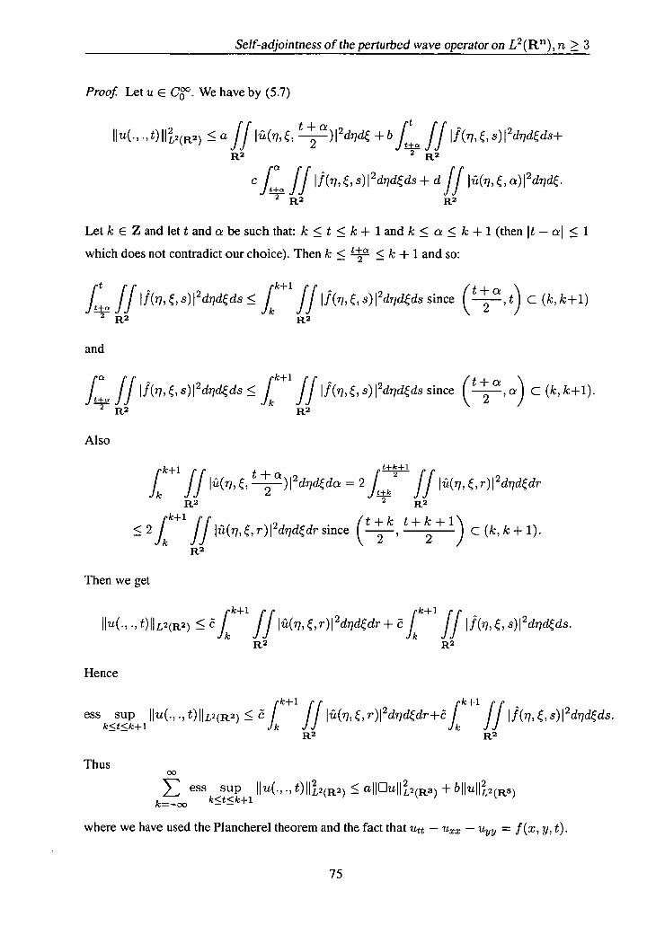
Self-adjoin tness of the perturbed wave operator on L 2 (Re), n > 3
Proof. Let u E C'°. We have by (5.7)
t) II2(R2) <aff Iu(m + a)I2d + bf ff If(m , s) I 2 thideds+
R2 2 R2
C , I f! I!(m , s)l 2dujdds + dff I2(m e a)I 2dd.
2 R2 R2
Let k E Z and let t and a be such that: k <t < k + 1 and k < a < k + 1 (then It - a I < 1
which does not contradict our choice). Then k < < k + 1 and so:
ffft k+1 /t+a \ If(Th,$)I2dI)deds < j ff IJ(me,$)l2d11cidssince 2 t) C (k, k+1)
2 R2 R2
and
fff If(m , s)l 2ddds < f ff J(m , s)f 2di1dds since (t + a, a) C (k, k+1). 2 R2 R2
Also
k+1
f ff I(m ± a)I2ddd 2 = 2 / jj ü(i, , r) 12 d7jd~dr J L±!
R2 2 R2
< 2Jk+1 (t+k t+k+1) ff Ju(me,r)I 2d7)ddr since , c(k,k+1)
k 2 2 R2
Then we get
Iu(, ., 0 11L2(R2) f
k+1
ff ü(i, , r)I 2dijddr + ofk
k±1 ff IJ(m , 8
)I2dideds. R2 R2
Hence
ess sup IIu(., ., t)IIL2(R2) < 0J
ff
Iu( i , , r)I2driddr+Ef
k k+1 ff
J(r, , 8
)I2didds. k<t<k+1
R2
Thus 00
2 <ajIDuI2 ess sup IIu(., ., t)11L2(R2) - lL2(R3) + bIIuII2(R3) k<t<k+1 k=—oo
where we have used the Plancherel theorem and the fact that Utt - - = f(x, y, t).
VAI
Self-adjoin tness of the perturbed wave operator on L 2 (Re), n > 3
Using the usual density argument allows us to obtain the desired result for M3 functions (see
the proof of Proposition 24). EN
Theorem 32. Let Li be the wave operator defined on L 2 (W). Let V be a real-valued function
Ik
k+ 1 such that sup IIV(., ., t)IIQ(R2)dt < oo. Then Li + V is self-adjointon V(L]).
keZ
Proof We have
00 k+1 IVuII2(R3) = i j fflv(x,y,t)u(x,y,t)I2dxdydt
k=—oo R2 CO k+1
i2 fk IIu(., ., t) 112 2(R2 ) IIV(., ., t) IIL°O(R2)dt. 1k=—oo
Hence
00 k+1 IVuII2(R3) ess sup IIu(., ., t)II2(R2) f IIV(., ., t)Il(R2)dt.
k=— oo k<t<k+1
So that
k+1 00
IVuII2(Ra) sup Jk IIV(., .,t)II(R2)dt ess sup IIu(., .,t)II2(R2)
kEZ k=— oo k<t~k+1
k+ 1 2 . <supf IIV(., ., t) IIL(R2 )dt (all LiuII2 L2(R3) + bIIuII
2 L2(R3))
kEZ k
where a can arbitrarily small (by the same argument). Hence L1+V is self-adjointon D(0). 0
Example 19. We show that Theorem 32 is stronger than Theorem 30 by giving an example. We
want a ço : R i-* R such that W 0 LOO (R),
supf
k+1 00 k+1
k'(t)I 2 dt <00 and >f I(t)I 2 dt = 00.
The condition on the right hand side of the last equation means that L 2 (R). We do not
want E L 2 (R) only because this case is already included in the class of Vs that was found
in Theorem 30.
76

Self-adjointness of the perturbed wave operator on L 2 (R'), n > 3
Fix - I < a < 0 and define Win each interval k <t <k + 1, k E Z, by
(t) = (t - k)a.
Then W is certainly not essentially bounded on R Moreover one has
Ik k+ 1
Ico(t)I2dt= jk+l
(t—k)2°dt= 2c+1
Hence
sup Ik+1 1 1
I(t)I 2 dt = Sup- <00. kEZJk kEZ 2 + 1 2a+ 1
And
E00
1 =00.
2a + 1 k=—oo
Now take V(x, y, t) o(t). Thus LI + V is seif-adjoint on
Remark 28. The V constructed in Example 19 does not satisfy the conditions of Proposition
33.
Again we have the same results in n -dimensions.
Proposition 35. For all a> 0, there exists b> 0 such that
00
ess sup II(.•., t)II2(Rn) ~ aIILJuIIL2(Rfl+1) + bIIuII2(Rn+1) k =— CIO k <t<k+1
for all u E
Theorem 33. Let LI be the wave operator defined on L2 (Rn1+ ). Let V be a real-valued tk+ 1
function such that sup] IIV(..., t)II)o(Rn)dt < 00. Then 0 + V is seif-adjoint on D(D). kEZ k
By going back to equation (5.4) we can do more, i.e., we have a better estimate than the one in
Proposition 30.
Proposition 36. For all a> 0, there exists b> 0 such that
esssup IIu(., .,t)IILr(R2) aIIDUIIL2(R3) + bIluIIL2(Rs), where 2< r <4. tER
for all u E M 3 .
77

Self-adjoin tness of the perturbed wave operator on L 2 (R11 ), ri > 3
We first need several lemmas.
Lemma 13 (Sobolev's inequality). For I e H' (R2 ) the inequality
Ill Il <aIIVfII2(R2)2 + bIIfII2(R2) holds for all 2 < q < oo.
For a proof see [7] (Theorem 8.5). We prefer here to use a proof which uses Fourier transforms
where we do not care about the constant a because we can always make it as small as we want.
Proof. Since f, , L(R 2 ), then by the Plancherel theorem we get: 1 l7f, f E L 2 (R 2 )
and hence 1, 1771f, L(R 2 ) which gives us:
(1 + lq l + II)f E L 2 (R2 ). Now let 2 < q < oo and let p be the conjugate of q (this implies
that 1 <p < 2). So:
IJ II IIIIP -LP(R2) - 1(1 + 1 711 + IIY'.( 1 + liiI + IeI)IJIIlL1(R2).
Then by Holder's inequality:
IIIIILP(R2) < 10 + IiI + IIY"IILr(R2)iI( 1 + liii + I0IJIIILs(R2)
where 1 + = 1. Let
C = 10 + IiI + IeIY'IILr(R2)
which is finite if pr > 2.
Now define r = 2 (this gives us pr > 2 so c is finite) and define s = (the exponents s and
r are conjugate).
We now use the fact that f e H 1 (R2 ). We have
10 + II + I0IfIIILs(R2) = (11(1+ 1771 + Il)P8IfIP9dde) R2
=
(
ff ( i + ii + 1)2 IJI2dde) = 1(1 + ini + II)IJIII2 (R2 ) . NR2
78

Self-adjoin tness of the perturbed wave operator on L 2 (Rr), n > 3
Thus for 1 <p < 2 we have:
ifiiL1(R2) cfl(l + iiil + 1i)1fl1iL2 (R2).
Hence 1
ifiiLp(R2) < C1
1' f liL2(R2) + c' 11 (ll + lei)ifIliL2 (R2 ).
Thus:
if IILP(R2 ) :!~ Cf llL2 (R2 ) + CIIVfIIL 2 (R2 ) 2 .
Thus by the Hausdorff-Young inequality (Theorem 5), we deduce that for 2 < q < oo:
III iILg(R2) < allVfllL2 (R2 ) 2 + bill llL2 (R2 ).
.
Lemma 14. Let w E L '
(R 2 ). Assume for all e > 0, there exist V,g such that w = V + g,
de and 1191Iq <; c, d being two constants. Then w E L(R 2 ) and
< Zc + d (5.10)
where = and < q < 00.
Proof. Let E,\ = {x: lu(x)I ~! Al. Then, since u= V + g
A E C {x: IV(x)l ~: }U{x: g(x)l > _
2 —}.
So that A
IEA 1 :!~- l{x: IV(x)i ~! > _lI. }i+l{x: g(x)i - V
Then using Chebyshev inequality
lEAi :!~ 4)c 211Vi1 +
But we have the freedom to choose any e(A) > 0. So take e(A) = Ab (b to be determined).
With this choice we obtain:
EAI < (4d2A21_2 + or
79
Self-adjoin tness of the perturbed wave operator on L 2 (Re), n > 3
)IEAI < 4d2 A 22 +
So in order that u belongs to L(R 2 ) it suffices to have:
sup[4d2P+21_2 + <oo.
which occurs ifb= -andp= _2_ 2+q Therefore,
2
IwIIp,w + cc'.
Finally, apply the same method as in the end of the proof of Theorem 3 to establish (5.10). 0
We shall now prove Proposition 36.
Proof. Let u e C°(R3 ). For a fixed t, let w(x, y) = u(x, y, t). We let
=
t \ 2 ~ e2 2ü (77, 2
+ o
)
cos [ (t_)]
— u(me,a) (5.11)
and
t sin\/172 + 2 (ck _s) ds
t
sin2+2(t—s)ds+J f(is) , ) = [ f(, , s)
2 + 2 + e2 2 t+Q j t+c
where f = Eu and c is yet to be chosen. We observe that both V and depend on c.
Note that ib = V + , by (5.4). It is clear that V E L2 (R2 ) and hence § E L 2 (R2 ). We let
V and g be their inverse Fourier transforms, so w = V + g. We aim to apply Lemma 14 by
showing that, given e> 0, we can choose & in such a way that 11V112 <dE and Jj9jj q < . Here,
q will satisfy 2 < q < oo, and c and d will be constants depending on 11u112 and 110u112. The
estimate for 1191I q will follow from Lemma 13 once we have shown that Vf e L 2 (R2 ) 2 with
suitable estimates.
We shall only consider the term ( 77, [ in (5.11) and the term
j1~ f(7), , s) sin \/?12±2(t8)
ds in (5.12) and we denote them by 17(, ) and ). The
proofs for the other two terms are similar.

Self-adjoin tness of the perturbed wave operator on L 2 (Re), n > 3
Let us start by showing that Vf E L 2 (R2 ) 2 . Since L2 (R2 ) and since
sin -,177 2 + 2 (t - s) sin /2 + 2 (t - s) E L°°(R 2 ),
- _____ _____
then —iij, — i L(R 2 ) which implies that Vg E L 2 (R 2 ) 2 since
IIVgII2(R2)2 = ff IVg(x, y)I 2 dxdy = IIII,2 (R2 ) 2
= I 77,e)I 2di1de+ffI(77,e)I 2d71ck, but
R2 R2
t t
s'n2+2(t—s)'d<J IJ(i,$)Ids.
I(m)I I If(m,$)II 2
.J 2 + 2 2
Then by using Cauchy-Schwarz
It It
Ff!V1
i, e)i ~ f If(m , s) 2 ds 1ds a If(m , s)I 2 dsIt - al I +a
And so t
a2t21t - aif I!(m, s)I 2ds. 2
By applying the same method one will also get
e2I(m )p2 < at - al l+Q IJ(m , 8)I 2 ds.
Now we choose a such that It - al <' . Hence 67
IIVgIIL2(R2)2 = ff Ii (m )I2dde
+ ff I(m )I 2diid
2a2 rr ~
--- JJ J± If(me,$)I2diidds. 62
R2 2
Thus
IIV9IIL2 (R2 ) 2 < — IIDUIIL2(R3). E
In a similar way one gets lIgIIL2(R2) --IlDullL2(R3). So for E > 1 we have II9II L2( R2) ~ eu
81

Self-adjointness of the perturbed wave operator on L 2 (Re), n > 3
II Dull L2(R3). In such case we get
II9IIL2(R2) II 1-]UIIL2(R3) S O 11911L(R2) :!~ IIDulIL2(R3) C C
by Lemma 13 where 2 < q < 00.
We also obtain the estimates when using J+c J(i, , s) Sfl V',?2±2(_s) ds. 2 V17
2+e
Now we come back to the case C < 1 after finding the bound for V which will be needed for
the case € < 1.
For V we have
( t+a\ = 2u
2 ) cos [2 + e2 (t a)]
, then
IIVII2(R2) 4ff I 2 (m ,t +2 a )I 2 thld
R2
and by integrating with respect to a E {a : It - al < I one obtains:
pt+ Iff t+a)I2ddda
~ 4 IIüII
L2(Rz)d a.
Jt_17 IIVIIa
~ 2 R2
Then there exists a E (t - t + ) such that
(R3 )
VII2(R2) 4 IIülI L2
and so IIVIIL2(R 2 ) dCIIuIIL2(R3).
The same applies to '2(7, , a) and we will get the same estimate.
Now for the case E < 1 one has to use § = 'ii' - V to obtain
II9Il L2(R2) :~ ö(IlwIIL2(R2) + IIVIIL2 (R2 )).
Then using the estimate for V, that is, IV IILZ(R2) dCIIuIjL2(a3) and Equation (5.8) give us
I191IL2(R2) < aIILJuIIL2(R3) + bIlullL2(R3) + CdIIUIIL 2(R3) :!5 ö(I1LuIIL2(R3) + bIIulIL2(R3))

Self-adjoin tness of the perturbed wave operator on L 2 (R"), n > 3
since E < 1. Thus
I9IILQ(R 2 ) < [IIDuIIL 2 (R3 ) + 11u11L2(R3)1.
So one has by Lemma 13
IWIIp,w :~: C11U115,2(R3) + CIIflUIIL2(R3). (5.13)
Equation (5.13) shows that w E LPW and since w e L (in fact, it belongs to L 2 ) then by (1. 1),
E L for 2 <r <p and
liWlir :~ CJIWII2,w + IIWIIp,w. (5.14)
We then get
IIWIILr(R2) :5 CWj2, w + allW11p,w !~ (IIwIl + IIEJUIIL2(R3) + IIUIIL2(R3)).
Now taking the essential supremum in t over R and using Proposition 30 shows that
esssupllu(., ., t)1JjrCp2 :5 CIIDUIIL 2 (R3 ) + CIIUIIL2(R3). (5.15) tER
Equation (5.15) holds whenever 2 < r < 4 since we have the constraints: p = , 2 q < 00
and 2 <r <p.
Finally, to obtain the result for arbitrary e M3 we use the usual approximation argument. E
We also have the result in higher dimensions.
Proposition 37. For all a> 0, there exists b> 0 such that
ess sup IIu(., ., t) IILr(Rn) aIIEIuIIL2(Rn+1) + bIIuIIL2(Rn+1) teR
for all u E -...
2n where n ~ 2 and where 2 < r
We are going to need another Sobolev's inequality in higher dimensions.
Proposition 38. Let n > 2. Let f e H' (R) then f e L(Rn')for 2 < q <and we
have:
IIfII < aIIVfIIL2(Rn)n +bIIfIIL 2 (Rn ) .
Remark 29. Observe that the case n = 2 gives us 2 < q < oo which was Lemma 13.
83

Self-adjoin tness of the perturbed wave operator on L 2 (Rn), n > 3
Remark 30. Observe that the proof in [7] (Theorem 8.3), is true even for the case q =
But for our problem we do not mind whether this q is sharp or not.
We also have the following theorem:
Theorem 34. Let 0 be the wave operator defined on L 2 (R3 ). Let V be a real -valued firnction
such that f IIV(., .,t)II$(R2)dt < oo where= - and 2 < r < 4. Then 0 + V is
self-adjoint on D(D).
Proof We have by the generalized Holder's inequality, for 1 = 1 +, 2 <r <4:
if V(x, y, t)u(x, y, t)I 2dxdy IV(., ., t) IL'(R 7 ) IIu(., ., t) IILr(R2)
R 2
2 11 2
esssupu(., ., t) 112 ., t)sp).
tER
Then by using Proposition 36 and by integrating with respect to t over R one gets
IVuII2(R3) <a 11 V(., .,
t)II$(R2)dt) II0uII + b Lf IIV(., ., t)IIS(R2)dt) IuII.
Since we can choose a small enough to have a f IIV(., ., t)II(R2)dt < 1 we conclude by the R
Kato-Rellich perturbation theorem that 0 + V is self-adjoint on D(D). 0
Theorem 35. Let n > 3. Let 0 be the wave operator defined on L 2 (R'). Let V be a
real-valued function such that f IIV(..., t)II5(Rfl)dt < oofor = - and 2 < r <
Then 0 + V is self-adjoint on D(0).
5.3 Counterexamples:
We show that there exists a o E L 2 (R) such that 0 E L 2 (Rr) and p L°°(R). We
do the same as for the second proof of Proposition 27. So one only need show that f = L2 (R " ) (in fact f is not in LP (R') for any 1 < p < oo). We have I+lt2-X2 21
If 112--
d_t_dx_2_ ... _d_x_ d_td_x_2_ ... d_x
( 1 +It2 —x—...—x f( 1 + 2 ++_2
t2_)2JR
_ _
84
Self-adjointness of the perturbed wave operator on L 2 (R'), n > 3
where D = {(x2, ...x, t) E R'Ix + ... + x, ~ t2 , t > O}. Now using "generalized polar
coordinates" we get
foo r 2 drdt f r.r 3drdt c fo 111112 ~ C
f oo
(1 + r2 - t2 ) 2 (1 + r2 - t2 ) 2
So
fo00 P00 rdr
fo
00
lfII ~.c t3dt / = Jt (1 + r2 - t 2 ) 2
2 tdt = 00.
Remark 31. As it is known for the Laplacian that tf W is in L 2 (R) such that L 2 (Rr)
then W E L°°(R") for n < 3 and E L(Rhl) for ii > 4 and where 2 < q < (c.f.
Theorem 6). Here we show the existence of a W e L 2 (R4) such that E L 2 (R4 ) and
while L 00 (R4 )
Proposition 39. Let W E L 2 (R 4 ) such that L 2 (R4 ). Then need not be essentially
bounded on R4 .
Proof One only need check that
(x ) y,z,t) f(x,y,z,t) =
L 1 +x2 +y +z2 +t2
(R4)
(which is an easy integration exercise). Then one has only to apply the same method as the
second proof of Proposition 27. Li
We also show that there exists a real-valued V E L2 C(Rn+ l) such that Li + V is not essentially
self-adjoint on C°. We have
Proposition 40. Let LI be the wave operator in n-dimensions defined on L 2 (R). Then there
exists a real-valued V E L 0 (R 1 ) such that Li + V is not essentially self -adjoint on Co .
Proof. We know by Example 16 that - - X1 is not essentially self-adjoint on CI (R) hence
the ODE: d2 —— fi(xi) - = ifi(xi)
x 1
has a non-zero solution in L 2 (R). We can say the same thing about:
d2 f2 (X2) - Xf2(X2) = if2(x2)
x2
F:i

Self-adjointness of the perturbed wave operator on L 2 (R"), n > 3
and d2
—--f(x) - X' fn = if (x) dx2
Also the following ODE has a non-zero solution in L 2 (R):
d2 —g(t) - t 4g(t) = _'9 (t)
or d2 Wt2g(t) + t4g(t) = +ig(t).
Multiplying each of the previous equations by the functions that are solutions to other equations.
For instance we multiply the first equation by f2 (x2)...f(x fl ).g(t) and so on. Then by adding
them up together, we have
/82 82 82 \ / n - - ... -
fi (xi) ... f(x)g(t) + - x) f i (x i ) ... f(x)g(t)
= (n + 1)ifi (x 1 ) ... f(x)g(t).
(5.16)
Take = fi (xj) ... f(x)g(t). Since f1,...,f,g are all in L2 (R) then p is in
L2 (R'') and is a solution of (5.16).
n So V(x i , ...,x, t) = t4 - E L(R') and
k=1
82 a2 a2 Exk -
k=1
is not essentially self-adjoint on C'°(R'). 0
5.4 Open problems
In this chapter there are more open problems than the previous one. They are:
is LI + V self-adjoint for V real-valued and in L 2 (R")? or essentially self-adjoint on Co ?
(see comments on Section 4.5, Question 1).
Assume V > 0 and such that V e 10C (Rn). Is 0 + V essentially self-adjoint on C000 ?
RE

Self-adjointness of the perturbed wave operator on L 2 (R"), n > 3
(also, see comments on Section 4.5).
Do we have M c BMO(R)? Observe that for n = 2 we do have M 2 C BMO(R 2 )
(see Remark 23).
If Question 3) has a negative answer then do we have Mn C L7 (R) for some p> 2? This
question may have a negative answer simply because we have not obtained any global estimate
of the type
Jjfjjp < auDi 112 + bllffl2,
for any p> 2 (p is far from infinity).
We say a few words concerning this question. There are known estimates for the wave equation
of the type
I IIq CIIDfIl
for some p and q (see [20] and [2 fl) but none of these is helpful for our purpose. For instance,
The estimate, J. Harmse gets in [20], is
Theorem 36. Assume n > 2. Suppose - = 2 and
n+1 2 1 n—i
<— < (5.17) 2nn+i q 2n
Then there is a constant C such that for every f E
II! II :!~ CIILIfII. (5.18)
If we want to apply this theorem to our problem one has to start with p = 2. But, with this
choice, q = 2(11±31) does not satisfy the condition (5.17) for any n > 2.
Also, in [21], it is proved that
Ill II MIIDuII
for q = 2(n+1) and p = 2(n+1) Observe that the case p = 2 cannot occur in this case. n+3
Finally, more 'Strichartz estimates' have been proved since Strichartz's paper [21] and one of
the important papers is [22].
We have by Proposition 37 an estimate which is true for 2 < r < So the natural
87

Self-adjoin tness of the perturbed wave operator on L 2 (R11 ), n > 3
question is: can we push the result beyond i.e., can we have the following estimate for
r> 2n and n>3:
ess sup IIu(..., t)IILr(Rn) < aIIDuIIL 2 (Rn+ 1 ) + bIIuIIL2(Rn+1)? teR
5.5 Conclusion
Finally, most of the results obtained in Chapters 4 and 5 (mainly Theorem 28, Proposition 25,
Proposition 27 (the first proof), Proposition 30, Proposition 37 and Theorem 35) form a paper
by myself [23] which has been accepted for publication.
88

References
E. Albrecht and P. G. Spain, "When Products of Self-adjoints Are Normal," Proceedings of the American Mathematical Society, vol. 128, no. 8, pp. 2509-2511, 2000.
M. H. Mortad, "An Application of the Putnam-Fuglede Theorem to Normal Products of Self-adjoint Operators," Proceedings of the American Mathematical Society, vol. 131, pp. 3135-3141, October 2003.
M.Reed and B.Simon, Methods of Modern Mathematical Physics, Vo12: Fourier Analysis and Self-adjointness. Academic Press, USA, first ed., 1975.
R. L. Wheeden and A. Zygmond, Measure and Integral. Marcel Dekker, 1977.
W. Rudin, Real and Complex Analysis. McGraw-Hill, third ed., 1987.
M. Reed and B. Simon, Methods of Modern Mathematical Physics, Vol]: Functional Analysis. Academic Press, first ed., 1972.
E. H. Lieb and M. Loss, Analysis. American Mathematical Society, first ed., 1997.
C. Sadosky, Interpolation of Operators and Singular Integrals. Marcel Dekker, 1979.
Y. Katznelson, Introduction to Harmonic Analysis. Dover Publications, Inc., second ed., 1976.
E. M. Stein, Singular Integrals and Differentiability Properties of Functions. Princeton University Press, 1970.
C. Zuily, Elements de distributions et d 'equations awr dérivées partielles. Dunod, 2002.
N. Akhiezer and I. Glazman, Theory of Linear Operators in Hilbert Space. Dover Publi-cations, Inc., 1993.
R. Meise and D. Vogt, Introduction to Functional Analysis. Oxford Science Publications, 1997.
W. Rudin, Functional Analysis. McGraw-Hill, second ed., 1991.
J. B. Conway, A Course in Functional Analysis. Springer-Verlag, first ed., 1985.
B. Fuglede, "A Commutativity Theorem for Normal Operators," Proc. National Acad. Sci, vol. 36, pp. 35-40, 1950.
C. R. Putnam, "On Normal Operators in Hilbert Space' Amer J. Math., vol. 73, no. 12, 1951.
A. Wintner, "On the Normalization of Characteristic Differentials in Continuous Spectra' Phys. Rev., vol. 72, pp. 516-517, 1947.
89
References
T. Kato, "Schrödinger Operators with Singular Potentials," Israel. J. Math., vol. 13, pp. 135-148, 1973.
J. Harmse, "On Lebesgue Space Estimates for the Wave Equation," Indiana University Mathematics Journal, vol. 39, no. 1-2, pp. 229-248, 1990.
R. S. Strichartz, "A Priori Estimates for the Wave Equation and Some Applications," Journal of Functional Analysis, vol. 5, pp. 218-235, 1970.
J. Ginibre and G. Velo, "Generalized Strichartz Inequalities for the Wave Equation," Jour-nal of Functional Analysis, vol. 133, pp. 50-68, 1995.
M. H. Mortad, "Self-Adjointness of the Perturbed Wave Operator on L 2 (R)," Proceed-ings of the American Mathematical Society, To appear.