Matlab stem function

figureY = linspace(-2*pi,2*pi,50);stem(Y)

figureX = linspace(0,2*pi,50)';Y = [cos(X), 0.5*sin(X)];stem(Y)

Histogram

Image Normalization

Normalization (image processing)

From Wikipedia, the free encyclopedia

In image processing, normalization is a process that changes the range of pixel intensity values. Applications include photographs with poor contrast due to glare, for example. Normalization is sometimes called contrast stretching or histogram stretching. In more general fields of data processing, such as digital signal processing, it is referred to as dynamic range expansion.[1]

The purpose of dynamic range expansion in the various applications is usually to bring the image, or other type of signal, into a range that is more familiar or normal to the senses, hence the term normalization. Often, the motivation is to achieve consistency in dynamic range for a set of data, signals, or images to avoid mental distraction or fatigue. For example, a newspaper will strive to make all of the images in an issue share a similar range of grayscale.

Normalization transforms an n-dimensional grayscale image with intensity values in the range (Min,Max), into a new image

with intensity values in the range (newMin,newMax).

The linear normalization of a grayscale digital image is performed according to the formula

For example, if the intensity range of the image is 50 to 180 and the desired range is 0 to 255 the process entails subtracting 50 from each of pixel intensity, making the range 0 to 130. Then each pixel intensity is multiplied by 255/130, making the range 0 to 255.

In our case Min=0 and Max=255

Matlab tutorial link: http://www.mathworks.com/matlabcentral/answers/26460-how-can-i-perform-gray-scale-image-normalization

Gaussian Filter

a=50; s=3;

g=fspecial('gaussian', [a a], s); g1=fspecial('gaussian', [11 11], 5);

Edge Detection methods Prewitt, Canny and Sobel with Matlab: I = imread('circuit.tif'); % I = imread('kids.tif'); figure, imshow(I);

BW1 = edge(I,'prewitt'); BW2 = edge(I,'canny'); BW3 = edge(I,'sobel'); figure, imshow(BW1); figure, imshow(BW2); figure, imshow(BW3);

Gaussian noise

>> a=imread('cameraman.tif');>> an=imnoise(a,'gaussian',0.01);>> figure,imshow(a);>> figure,imshow(an);>> sigma=3;>> cutoff=ceil(3*sigma);>> h=fspecial('gaussian', 2*cutoff+1,sigma);>> out=conv2(double(a),double(h),'same');>> figure, imshow(out);>> figure, imshow(out/256);>> out1=conv2(double(an),double(h),'same');>> figure, imshow(out1/256);>> surf(1:2*cutoff+1,1:2*cutoff+1,h);

Blurring and Sharpening

I = imread('cameraman.tif'); subplot(2,2,1);imshow(I);title('Original Image'); H = fspecial('motion',20,45); MotionBlur = imfilter(I,H,'replicate'); subplot(2,2,2);imshow(MotionBlur);title('Motion Blurred Image'); H = fspecial('disk',10); blurred = imfilter(I,H,'replicate'); subplot(2,2,3);imshow(blurred);title('Blurred Image'); H = fspecial('unsharp'); sharpened = imfilter(I,H,'replicate'); subplot(2,2,4);imshow(sharpened);title('Sharpened Image');

OpenCV installation Instructions

For Windows use this link:

http://docs.opencv.org/3.0-last-rst/doc/tutorials/introduction/windows_install/windows_install.html

For Linux this one:

http://docs.opencv.org/3.0-last-rst/doc/tutorials/introduction/linux_install/linux_install.html

In order to run a Java OpenCV program with Netbeans:

1. Add the openCV-310.jar to the libraries and

2. Go to program properties and add the java.library.path like in step 2.

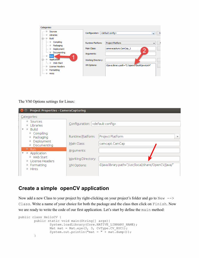
The VM Options settings for Linux:

Create a simple openCV application

Now add a new Class to your project by right-clicking on your project’s folder and go to New -->

Class. Write a name of your choice for both the package and the class then click on Finish. Now

we are ready to write the code of our first application. Let’s start by define the main method:

public class HelloCV { public static void main(String[] args){ System.loadLibrary(Core.NATIVE_LIBRARY_NAME); Mat mat = Mat.eye(3, 3, CvType.CV_8UC1); System.out.println("mat = " + mat.dump()); }

}

First of all we need to load the OpenCV Native Library previously set on our project.

System.loadLibrary(Core.NATIVE_LIBRARY_NAME);

Then we can define a new Mat.

Note

The class Mat represents an n-dimensional dense numerical single-channel or multi-channel array. It can be used to store real or complex-valued vectors and matrices, grayscale or color images, voxel volumes, vector fields, point clouds, tensors, histograms. For more details check out the OpenCV page.

Mat mat = Mat.eye(3, 3, CvType.CV_8UC1);

The Mat.eye represents a identity matrix, we set the dimensions of it (3x3) and the type of its

elements.

As you can notice, if you leave the code just like this, you will get some error; this is due to the fact that eclipse can’t resolve some variables. You can locate your mouse cursor on the words that seem to

be errors and wait for a dialog to pop up and click on the voice Import.... If you do that for all the

variables we have added to the code the following rows:

import org.opencv.core.Core;import org.opencv.core.CvType;import org.opencv.core.Mat;

http://homepages.inf.ed.ac.uk/rbf/HIPR2/sobel.htm

ConvolutionConvolution is a simple mathematical operation which is fundamental to many common image processing operators. Convolution provides a way of `multiplying together' two arrays of numbers, generally of different sizes, but of the same dimensionality, to produce a third array of numbers of the same dimensionality. This can be used in image processing to implement operators whose output pixel values are simple linear combinations of certain input pixel values.

In an image processing context, one of the input arrays is normally just a graylevel image. The second array is usually much smaller, and is also two-dimensional (although it may be just a single pixel thick), and is known as the kernel. Figure 1 shows an example image and kernel that we will use to

Netbeans simple OpenCV Java Program

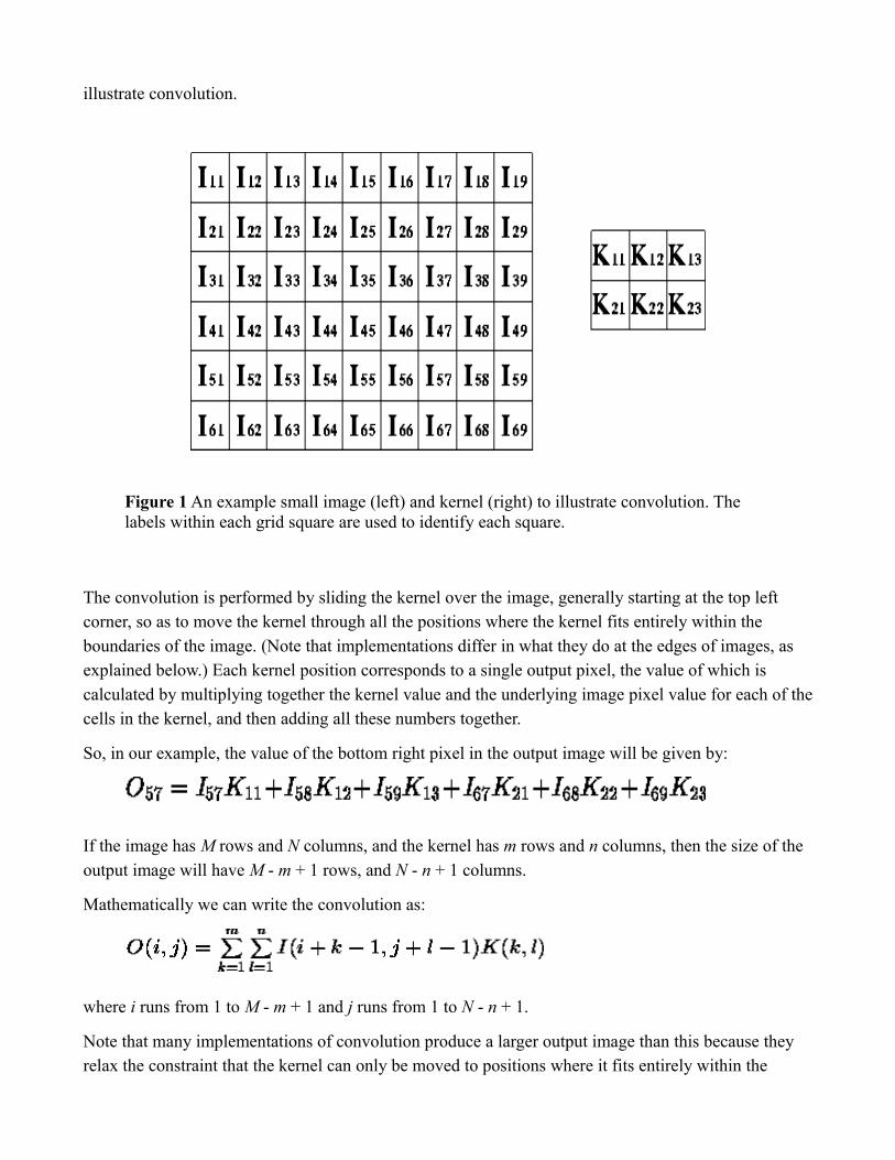
illustrate convolution.

Figure 1 An example small image (left) and kernel (right) to illustrate convolution. The labels within each grid square are used to identify each square.

The convolution is performed by sliding the kernel over the image, generally starting at the top left corner, so as to move the kernel through all the positions where the kernel fits entirely within the boundaries of the image. (Note that implementations differ in what they do at the edges of images, as explained below.) Each kernel position corresponds to a single output pixel, the value of which is calculated by multiplying together the kernel value and the underlying image pixel value for each of thecells in the kernel, and then adding all these numbers together.

So, in our example, the value of the bottom right pixel in the output image will be given by:

If the image has M rows and N columns, and the kernel has m rows and n columns, then the size of the output image will have M - m + 1 rows, and N - n + 1 columns.

Mathematically we can write the convolution as:

where i runs from 1 to M - m + 1 and j runs from 1 to N - n + 1.

Note that many implementations of convolution produce a larger output image than this because they relax the constraint that the kernel can only be moved to positions where it fits entirely within the

image. Instead, these implementations typically slide the kernel to all positions where just the top left corner of the kernel is within the image. Therefore the kernel `overlaps' the image on the bottom and right edges. One advantage of this approach is that the output image is the same size as the input image.Unfortunately, in order to calculate the output pixel values for the bottom and right edges of the image, it is necessary to invent input pixel values for places where the kernel extends off the end of the image. Typically pixel values of zero are chosen for regions outside the true image, but this can often distort the output image at these places. Therefore in general if you are using a convolution implementation that does this, it is better to clip the image to remove these spurious regions. Removing n - 1 pixels from the right hand side and m - 1 pixels from the bottom will fix things.

Convolution can be used to implement many different operators, particularly spatial filters and feature detectors. Examples include Gaussian smoothing and the Sobel edge detector.

Interactive ExperimentationYou can interactively experiment with this operator by clicking here.

8.2. Convolution Matrix 8. Generic Filters

8.2. Convolution Matrix

8.2.1. Overview

Here is a mathematician's domain. Most of filters are using convolution matrix. With the Convolution Matrix filter, if the fancy takes you, you can build a custom filter.

What is a convolution matrix? It's possible to get a rough idea of it without using mathematical tools that only a few ones know. Convolution is the treatment of a matrix by another one which is called “kernel”.

The Convolution Matrix filter uses a first matrix which is the Image to be treated. The image is a bi-dimensional collection of pixels in rectangular coordinates. The used kernel depends on the effect you want.

GIMP uses 5x5 or 3x3 matrices. We will consider only 3x3 matrices, they are the most used and they are enough for all effects you want. If all border values of a kernel are set to zero, then system will consider it as a 3x3 matrix.

The filter studies successively every pixel of the image. For each of them, which we will call the “initial pixel”, it multiplies the value of this pixel and values of the 8 surrounding pixels by the kernel corresponding value. Then it adds the results, and the initial pixel is set to this final result value.

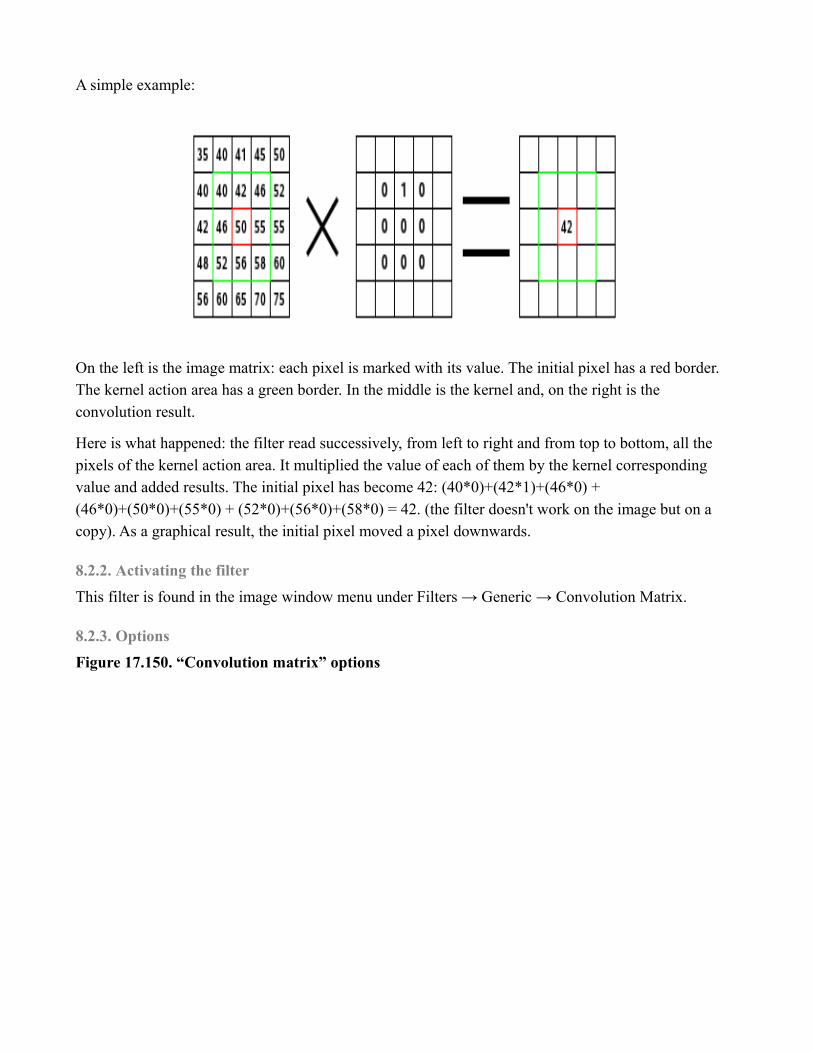
A simple example:

On the left is the image matrix: each pixel is marked with its value. The initial pixel has a red border. The kernel action area has a green border. In the middle is the kernel and, on the right is the convolution result.

Here is what happened: the filter read successively, from left to right and from top to bottom, all the pixels of the kernel action area. It multiplied the value of each of them by the kernel corresponding value and added results. The initial pixel has become 42: (40*0)+(42*1)+(46*0) + (46*0)+(50*0)+(55*0) + (52*0)+(56*0)+(58*0) = 42. (the filter doesn't work on the image but on a copy). As a graphical result, the initial pixel moved a pixel downwards.

8.2.2. Activating the filter

This filter is found in the image window menu under Filters → Generic → Convolution Matrix.

8.2.3. Options

Figure 17.150. “Convolution matrix” options

Matrix

This is the 5x5 kernel matrix: you enter wanted values directly into boxes.

Divisor

The result of previous calculation will be divided by this divisor. You will hardly use 1, which lets result unchanged, and 9 or 25 according to matrix size, which gives the average of pixel values.

Offset

This value is added to the division result. This is useful if result may be negative. This offset may be negative.

Border

When the initial pixel is on a border, a part of kernel is out of image. You have to decide what filter must do:

From left: source image, Extend border, Wrap border, Crop border

Extend

This part of kernel is not taken into account.

Wrap

This part of kernel will study pixels of the opposite border, so pixels disappearing from one side reappear on the other side.

Crop

Pixels on borders are not modified, but they are cropped.

Channels

You can select there one or several channels the filter will work with.

Normalise

If this option is checked, The Divisor takes the result value of convolution. If this result is equal to zero (it's not possible to divide by zero), then a 128 offset is applied. If it is negative (a negative color is not possible), a 255 offset is applied (inverts result).

Alpha-weighting

If this option is not checked, the filter doesn't take in account transparency and this may be cause of some artefacts when blurring.

8.2.4. Examples

Design of kernels is based on high levels mathematics. You can find ready-made kernels on the Web.

Here are a few examples:

Figure 17.151. Sharpen

Figure 17.152. Blur

Figure 17.153. Edge enhance

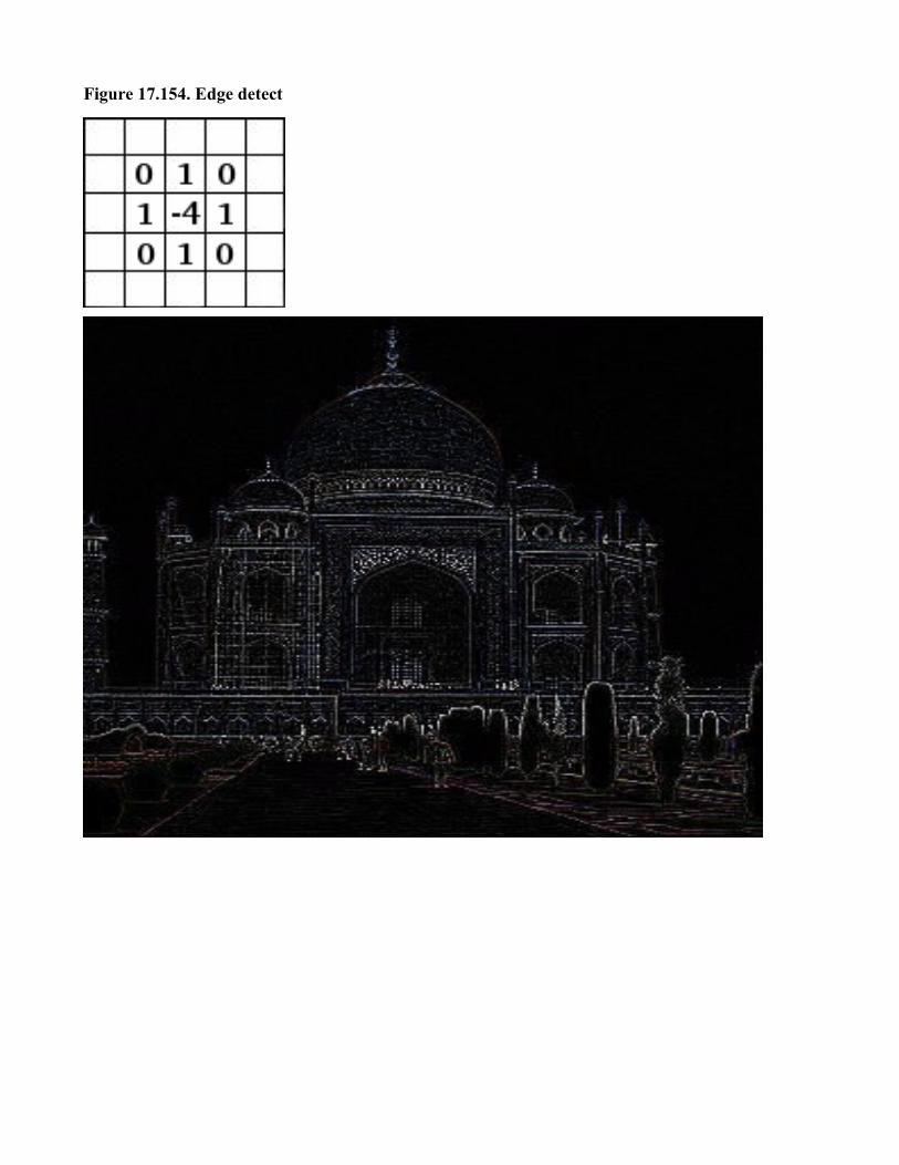
Figure 17.154. Edge detect

Figure 17.155. Emboss