northumbria research linknrl.northumbria.ac.uk/27037/1/tom_watts_thesis_2015_small_final.pdf ·...
TRANSCRIPT

Northumbria Research Link
Citation: Watts, Tom (2015) Influence of stratigraphy and heterogeneity on simulated microwave brightness temperatures of shallow snowpacks. Doctoral thesis, Northumbria University.
This version was downloaded from Northumbria Research Link: http://nrl.northumbria.ac.uk/27037/
Northumbria University has developed Northumbria Research Link (NRL) to enable users to access the University’s research output. Copyright © and moral rights for items on NRL are retained by the individual author(s) and/or other copyright owners. Single copies of full items can be reproduced, displayed or performed, and given to third parties in any format or medium for personal research or study, educational, or not-for-profit purposes without prior permission or charge, provided the authors, title and full bibliographic details are given, as well as a hyperlink and/or URL to the original metadata page. The content must not be changed in any way. Full items must not be sold commercially in any format or medium without formal permission of the copyright holder. The full policy is available online: http://nrl.northumbria.ac.uk/pol i cies.html

Influence of Stratigraphy andHeterogeneity on Simulated
Microwave BrightnessTemperatures of Shallow Snowpacks
T P Watts
PhD
2015

Influence of Stratigraphy andHeterogeneity on Simulated
Microwave BrightnessTemperatures of Shallow Snowpacks
Thomas Peter Watts
A thesis submitted in partialfulfilment of the requirements of the Universityof Northumbria at Newcastle for the degree of
Doctor of Philosophy
This research was undertaken in theFaculty of Engineering and Environment
November 2015
ii

AbstractSnow accumulation has potential climatological, hydrological and ecological im-pacts at a global scale. Satellite passive microwave radiometers have the po-tential to provide snow accumulation data with a historical record of over 30years, however, current data products contain unknown uncertainty and error.Snowpack stratigraphy is the spatial variation in snowpack properties causedby the layered nature of the snowpack. Snowpack stratigraphy influences theaccuracy and increases uncertainty in simulations of microwave emission fromsnow which in turn increases uncertainty in satellite derived estimates of snowwater equivalent using microwave radiometers.
Two methods were developed to help better quantify snowpack stratigraphy. Animproved technique for characterising snowpack stratigraphy within a snow trenchwas developed. Secondly a new method was developed to quantify the density ofice layers that form in snowpacks with known error and uncertainty.
Snowpack stratigraphy was characterised using the improved technique acrossthe Trail Valley Creek watershed in the Canadian Northwest Territories. Two50 m trenches and eleven 5 m trenches were dug across the range of landcovertypes found in the watershed. This dataset allowed layer boundary roughnessto be characterised and the properties of snow layers to be mapped with anunprecedented level of accuracy.
Ice lens density was measured 60 times at three locations in the Arctic and mid-latitudes at locations with coincident ground based radiometer measurements.The impact that accurate parameterisation of density has on modelled estimatesof brightness temperature was quantified.
Simulations of microwave brightness temperatures were conducted using snowemission models at all locations. The output of these simulations, and comparisonto ground based observations where available, allowed for the characterisation ofvariability in brightness temperature simulations caused by stratigraphic hetero-geneity. The findings presented in this thesis will inform research aiming to bettercharacterise the satellite error budget. Improvements in this area helps improveglobal snow mass and snow accumulation estimates.

Contents
Abstract i
Contents ii
List of Figures vi
List of Tables ix
Acknowledgements x
Declaration of Authorship xii
1 Introduction 11.1 Snow at a global scale . . . . . . . . . . . . . . . . . . . . . . . . 11.2 Measuring Snow Water Equivalent . . . . . . . . . . . . . . . . . 51.3 Snowpack variability and stratigraphy . . . . . . . . . . . . . . . . 91.4 Quantifying variation in snowpack
stratigraphy . . . . . . . . . . . . . . . . . . . . . . . . . . . . . . 111.5 Aims . . . . . . . . . . . . . . . . . . . . . . . . . . . . . . . . . . 111.6 Thesis structure . . . . . . . . . . . . . . . . . . . . . . . . . . . . 14
2 Origins of microwave signatures in tundra snowpacks 152.1 In situ quantification methods of natural snow cover . . . . . . . . 15
2.1.1 Snow pit measurements . . . . . . . . . . . . . . . . . . . . 162.1.2 Measuring spatial variability . . . . . . . . . . . . . . . . . 172.1.3 Emerging Methods . . . . . . . . . . . . . . . . . . . . . . 172.1.4 NIR Photography . . . . . . . . . . . . . . . . . . . . . . . 18
2.2 General Principles of Passive microwaveremote sensing . . . . . . . . . . . . . . . . . . . . . . . . . . . . 20
2.3 Snow emission modelling . . . . . . . . . . . . . . . . . . . . . . . 222.4 Passive microwave remote sensing of snow . . . . . . . . . . . . . 24
ii

Contents
2.4.1 Principle . . . . . . . . . . . . . . . . . . . . . . . . . . . . 242.4.2 Retrieval Algorithms . . . . . . . . . . . . . . . . . . . . . 25
2.4.2.1 Empirical . . . . . . . . . . . . . . . . . . . . . . 262.4.2.2 Modified Empirical . . . . . . . . . . . . . . . . . 272.4.2.3 Model based . . . . . . . . . . . . . . . . . . . . 30
2.5 Challenges in the application of retrievalalgorithms . . . . . . . . . . . . . . . . . . . . . . . . . . . . . . . 312.5.1 Layering . . . . . . . . . . . . . . . . . . . . . . . . . . . . 322.5.2 Variability in Stratigraphy . . . . . . . . . . . . . . . . . . 332.5.3 Depth Hoar . . . . . . . . . . . . . . . . . . . . . . . . . . 352.5.4 Wind re-distribution . . . . . . . . . . . . . . . . . . . . . 362.5.5 Melt and rain-on-snow events . . . . . . . . . . . . . . . . 36
3 Digitising Snowpack Stratigraphy with Improved Accuracy 393.1 Research aims and objectives . . . . . . . . . . . . . . . . . . . . 393.2 Development of stratigraphy digitisation
method . . . . . . . . . . . . . . . . . . . . . . . . . . . . . . . . 423.2.1 Preparing the NIR images . . . . . . . . . . . . . . . . . . 433.2.2 Extracting snow stratigraphy information from NIR snow
trench photography . . . . . . . . . . . . . . . . . . . . . . 443.2.3 Calculating positions in digital images in cm . . . . . . . . 463.2.4 Accounting for artefacts in digitised snow stratigraphy in-
formation . . . . . . . . . . . . . . . . . . . . . . . . . . . 503.2.4.1 Applying smoothing . . . . . . . . . . . . . . . . 553.2.4.2 Smoothing Optimisation . . . . . . . . . . . . . . 55
3.2.5 Assigning snowpack properties to digitisedstratigraphy . . . . . . . . . . . . . . . . . . . . . . . . . . 58
3.3 Field Methods . . . . . . . . . . . . . . . . . . . . . . . . . . . . . 603.3.1 Field Site . . . . . . . . . . . . . . . . . . . . . . . . . . . 60
3.4 Results . . . . . . . . . . . . . . . . . . . . . . . . . . . . . . . . . 613.4.1 Variation in snowpack properties and characteristics . . . . 623.4.2 Variation in n-HUT model Tb . . . . . . . . . . . . . . . . 72
3.5 Discussion . . . . . . . . . . . . . . . . . . . . . . . . . . . . . . . 78
4 Improved measurement of ice layer densities and application insnow microwave emission models 814.1 Aims . . . . . . . . . . . . . . . . . . . . . . . . . . . . . . . . . . 814.2 Measurements of ice layer density . . . . . . . . . . . . . . . . . . 82
4.2.1 Development of ice density measurement method . . . . . 824.2.2 Methodological error . . . . . . . . . . . . . . . . . . . . . 854.2.3 Field Measurements . . . . . . . . . . . . . . . . . . . . . 87
4.2.3.1 Ice layer measurements . . . . . . . . . . . . . . . 87
iii

Contents
4.2.3.2 Brightness Temperature observations . . . . . . . 894.3 Results: Ice layer measurements . . . . . . . . . . . . . . . . . . . 89
4.3.1 Ice layer bubble size and thickness . . . . . . . . . . . . . . 894.3.2 Ice layer density . . . . . . . . . . . . . . . . . . . . . . . . 904.3.3 Error in measured density . . . . . . . . . . . . . . . . . . 91
4.4 Simulation of brightness temperatures using measured ice density 964.4.1 Model Initialisation . . . . . . . . . . . . . . . . . . . . . . 96
4.4.1.1 DMRT-ML . . . . . . . . . . . . . . . . . . . . . 964.4.1.2 MEMLS . . . . . . . . . . . . . . . . . . . . . . . 98
4.5 Results: Brightness temperature simulations . . . . . . . . . . . . 994.5.1 Model Sensitivity to ice layer properties . . . . . . . . . . 100
4.5.1.1 MEMLS . . . . . . . . . . . . . . . . . . . . . . . 1004.5.1.2 DMRT-ML . . . . . . . . . . . . . . . . . . . . . 101
4.5.2 Model optimisation using ice layer density . . . . . . . . . 1034.5.3 Effect of ice layer density on polarisation and gradient ratios105
4.6 Discussion and Conclusions . . . . . . . . . . . . . . . . . . . . . 108
5 Snow Trenches in Inuvik 1105.1 Introduction . . . . . . . . . . . . . . . . . . . . . . . . . . . . . . 1105.2 Aims and Objectives . . . . . . . . . . . . . . . . . . . . . . . . . 1115.3 Field Methods . . . . . . . . . . . . . . . . . . . . . . . . . . . . . 112
5.3.1 Field Site . . . . . . . . . . . . . . . . . . . . . . . . . . . 1125.3.2 Field Measurements . . . . . . . . . . . . . . . . . . . . . 115
5.3.2.1 Application of NIR trenches to distances >50 m . 1155.3.2.2 Trench measurements . . . . . . . . . . . . . . . 116
5.4 Results and Analysis . . . . . . . . . . . . . . . . . . . . . . . . . 1195.4.1 Snowpack characteristics and variability . . . . . . . . . . 119
5.4.1.1 Snowpack variation over 50 m . . . . . . . . . . . 1195.4.2 Boundary Roughness Variability . . . . . . . . . . . . . . . 1235.4.3 Variation in simulated brightness temperatures . . . . . . 1265.4.4 Sample size to accurately simulate brightness temperature 128
5.4.4.1 Differences between sites . . . . . . . . . . . . . . 1335.5 Discussion . . . . . . . . . . . . . . . . . . . . . . . . . . . . . . . 1355.6 Summary . . . . . . . . . . . . . . . . . . . . . . . . . . . . . . . 137
5.6.1 Quantify layer thickness and boundary roughnessvariability . . . . . . . . . . . . . . . . . . . . . . . . . . . 138
5.6.2 Quantifying the impact of spatial variability of stratigraphyon Snow Microwave Emission Models . . . . . . . . . . . . 138
5.6.3 Determine what the minimum subset size is . . . . . . . . 139
6 Synopsis 1406.1 Summary . . . . . . . . . . . . . . . . . . . . . . . . . . . . . . . 140
iv

Contents
6.1.1 Snowpack stratigraphy . . . . . . . . . . . . . . . . . . . . 1416.1.2 Ice layer Density . . . . . . . . . . . . . . . . . . . . . . . 144
6.2 Future Work . . . . . . . . . . . . . . . . . . . . . . . . . . . . . . 147
148
v

List of Figures
1.1 Feedbacks in the Arctic . . . . . . . . . . . . . . . . . . . . . . . . 31.2 World population dependent on snow melt . . . . . . . . . . . . . 41.3 Extreme runoff events in the Northern Hemisphere . . . . . . . . 41.4 Example SWE retrieval assimilation scheme . . . . . . . . . . . . 8
2.1 Plank’s law . . . . . . . . . . . . . . . . . . . . . . . . . . . . . . 212.2 Effect of Grain Size on 37 GHz (V-pol) brightness temperature . . 272.3 Variation in penetration depth between different frequencies . . . 29
3.1 An example of NIR snow trench photography . . . . . . . . . . . 433.2 NIR images stitched together to show stratigraphy across trench 443.3 Position of digitalized snow layers in pixels . . . . . . . . . . . . . 453.4 Applying the canny edge detection algorithm to a measuring staff 473.5 Test layer translated using the per pixel translation . . . . . . . . 513.6 Un-smoothed snow layers quantified from NIR photography of snow
trench wall, Red box indicates area displayed in Figure 3.7 . . . . 523.7 Random roughness over the section highlighted in Figure 3.6, layers
numbered in descending order according to height . . . . . . . . . 533.8 Histogram of the random roughness metric for a sample snow layer 543.9 Random roughness over the section highlighted in Figure 3.6 after
smoothing has been applied . . . . . . . . . . . . . . . . . . . . . 563.10 Impact of smoothing on whole trench . . . . . . . . . . . . . . . . 573.11 Locations of density measurements placed automatically on snow-
pack stratigraphy . . . . . . . . . . . . . . . . . . . . . . . . . . . 593.12 Locations where trench sampling took place . . . . . . . . . . . . 613.13 Difference in range of total snowpack SWE and Depth measure-
ments across entire trench . . . . . . . . . . . . . . . . . . . . . . 633.14 Variation in snow properties within and between layers in each
trench. . . . . . . . . . . . . . . . . . . . . . . . . . . . . . . . . . 643.15 Snow microstructure and grain type symbols used in this thesis
(classification/symbols from Fierz et al. (2009)) . . . . . . . . . . 653.16 Stratigraphy and snowpack properties of Trench 1, ice crusts are
marked in red on the top image . . . . . . . . . . . . . . . . . . . 66
vi

List of Figures
3.17 Stratigraphy and snowpack properties of Trench 2, ice crusts aremarked in red on the top image . . . . . . . . . . . . . . . . . . . 67
3.18 Stratigraphy and snowpack properties of Trench 3, ice crusts aremarked in red on the top image . . . . . . . . . . . . . . . . . . . 68
3.19 Stratigraphy and snowpack properties of Trench 4, ice crusts aremarked in red on the top image . . . . . . . . . . . . . . . . . . . 69
3.20 Stratigraphy from trenches 1 and 2, showing how they relate toeach other in three dimensions. . . . . . . . . . . . . . . . . . . . 70
3.21 Boxplots for random roughness. . . . . . . . . . . . . . . . . . . . 713.22 Histograms showing the distribution of Brightness Temperatures
simulations for Trench 1 . . . . . . . . . . . . . . . . . . . . . . . 743.23 Histograms showing the distribution of Brightness Temperatures
simulations for Trench 2 . . . . . . . . . . . . . . . . . . . . . . . 753.24 Histograms showing the distribution of Brightness Temperatures
simulations for Trench 3 . . . . . . . . . . . . . . . . . . . . . . . 763.25 Histograms showing the distribution of Brightness Temperatures
simulations for Trench 4 . . . . . . . . . . . . . . . . . . . . . . . 77
4.1 Ice layer density measurement flow chart . . . . . . . . . . . . . . 834.2 Ice volume measurement photographs . . . . . . . . . . . . . . . . 844.3 Ice layer density histogram . . . . . . . . . . . . . . . . . . . . . . 914.4 Schematic of ice layer layer porosity model . . . . . . . . . . . . . 934.5 3d plot showing the influence of ice layer density . . . . . . . . . . 944.6 Observed and modelled snowpack at North Bay, explanation of
snow symbols in figure 3.15 . . . . . . . . . . . . . . . . . . . . . 984.7 Sensitivity of MEMLS to ice layer properties . . . . . . . . . . . . 1014.8 Sensitivity of DMRT-ML to ice layer properties . . . . . . . . . . 1024.9 Difference between modelled and observed brightness temperatures
with changing density for MEMLS . . . . . . . . . . . . . . . . . 1044.10 Difference between modelled and observed brightness temperatures
with changing density for DMRT-ML . . . . . . . . . . . . . . . . 1054.11 Effect of density on gradient ratio . . . . . . . . . . . . . . . . . . 1074.12 Effect of density on polarisation ratio . . . . . . . . . . . . . . . . 107
5.1 Map of location of Trail Valley Creek . . . . . . . . . . . . . . . . 1135.2 Meteorological data from the winter of 2012-2013 from the main
tundra met site in Trail Valley Creek . . . . . . . . . . . . . . . . 1145.3 Photo showing collection of snowpack data from Trench 4 in Trail
Valley creek . . . . . . . . . . . . . . . . . . . . . . . . . . . . . . 1165.4 Map of trench locations in Trail Valley Creek . . . . . . . . . . . 1185.5 Example of a spherical model fitted to the semivariogram data points1225.6 Semivariogram of snow layer thickness within trenches excavated
in Trail Valley Creek . . . . . . . . . . . . . . . . . . . . . . . . . 122
vii

List of Figures
5.7 Layer boundary roughness compared to proportional layer bound-ary height . . . . . . . . . . . . . . . . . . . . . . . . . . . . . . . 124
5.8 Layer boundary roughness compared to proportional layer bound-ary height with generalised fit . . . . . . . . . . . . . . . . . . . . 125
5.9 Comparison of trench data and distributed pit data . . . . . . . . 1275.10 Semi-variograms of modelled brightness temperatures . . . . . . . 1285.11 Histograms of Brightness Temperature simulations of Trench 4 . . 1295.12 Increasing the sample size and comparing the sample mean to the
population mean for trench 4 . . . . . . . . . . . . . . . . . . . . 1325.13 Mean brightness temperatures at different sites around Trail Valley
Creek . . . . . . . . . . . . . . . . . . . . . . . . . . . . . . . . . 134
6.1 Flow chart of the key areas used in data assimilation schemes whichare improved or addressed by the work in this thesis . . . . . . . . 141
6.2 Conceptual diagram of the areas improved by this research . . . . 1456.3 Comparison of a typical brightness temperature distribution for 19
GHz H-pol when ice layers are a) absent and b) present . . . . . . 145
viii

List of Tables
2.1 Passive Microwave satellite radiometer missions suitable for snowremote sensing . . . . . . . . . . . . . . . . . . . . . . . . . . . . 22
3.1 Simulated brightness temperatures from using bulk snowpack prop-erties . . . . . . . . . . . . . . . . . . . . . . . . . . . . . . . . . . 72
3.2 Simulated brightness temperatures from using averaged snowpackbased on trench data . . . . . . . . . . . . . . . . . . . . . . . . . 73
3.3 Mean and standard deviations of simulated brightness tempera-tures from trenches . . . . . . . . . . . . . . . . . . . . . . . . . . 73
3.4 Differences in simulated brightness temperatures between pairs oforthogonal trenches . . . . . . . . . . . . . . . . . . . . . . . . . . 74
4.1 Ice layer thicknesses and bubble sizes . . . . . . . . . . . . . . . . 904.2 Ice layer density measurements, (all values have been corrected to
account for the measured −0.19cm3 bias in volume) . . . . . . . . 904.3 Summary of range of input and initialisation parameters across all
model runs . . . . . . . . . . . . . . . . . . . . . . . . . . . . . . . 974.4 Observed brightness temperatures . . . . . . . . . . . . . . . . . . 103
5.1 Table of all measurements made at trenches their lengths andreference to locations in Figure 5.4 . . . . . . . . . . . . . . . . . 119
5.2 Range (cm) at sill for top middle and bottom layer thicknesses ineach trench . . . . . . . . . . . . . . . . . . . . . . . . . . . . . . 123
5.3 Coefficients for fitted boundary roughness relationships . . . . . . 1255.4 Range (lag distance) at sill of semivariograms . . . . . . . . . . . 1275.5 Minimum sample size to achieve population mean for trench based
brightness temperature simulations . . . . . . . . . . . . . . . . . 1315.6 Comparison between the simulated brightness temperatures and
required minimum sample size between different groups of sites . . 134
ix

Acknowledgements
Writing this thesis has proved to be a significant personal challenge, however, it
would not have been possible without the support of a great many people. Thank
you to all those who helped make my PhD a positive, exciting, interesting, at times
even fun, experience. In particular I’d like to acknowledge:
The help and guidance of Nick Rutter and Melody Sandells, for their insight,
encouragement and enthusiasm, whether things were going well or poorly. For
sharing your ideas, helping me come up with my own and leading me to ask new
questions when I was running out of steam.
Everyone I worked with at Environment Canada, Chris Derksen for seeing through
the noise and knowing what matters...and then encouraging me to do that stuff!
Thank you for your family’s incredible hospitality, I will not forget the brisket
in a hurry. Pete, Buffy (and Sheriff), thank you for letting me turn your empty
apartment and basement into, (only marginally) less empty homes, and for your
friendship and hospitality. Arvids, thanks for sorting everything out, and for
passing on a tiny fraction of your field expertise... I know I’ve forgotten something!
The constructive criticism, feedback and helpful comments from my examiner
Juha Lemmetyinen whose input has vastly improved the quality of this thesis.
Also Ben Brock for his input during my viva and John Woodward for proof
reading early versions of chapters of this thesis and for ongoing input and advice
throughout my PhD.
x

The support of Richard Essery, Dave Thomas, Dave Halpin and everyone from
Sherbrooke, Waterloo and Boise Universities who helped collect data and pass
the time in the hut at trail valley creek.
My friends in Newcastle, for their endless distractions, - in many ways surfing
is the perfect PhD sport. And from Chippenham and Sheffield, for providing
excellent excuses to get out of the North East when things got a bit too Northern.
Finally, the support of my family, firstly the Stephensons for being my home
in the North East. Edd and Jodie, thank you for always being there for me
when disaster struck or when it didn’t and for being the best brother and sister
anyone could ask for. But most of all my parents for the lifelong support and for
encouraging me to follow my passions, (despite the comparative lack of financial
compensation). For your interest in my work and happiness and for motivating
me to do more when times were good, and to ’just do something’ when times
were bad. Without any of you in my lives I would never have made it this far.
This work was supported by a Northumbria University RDF studentship and the
Canadian Natural Science and Engineering Research Council; field activities were
funded by Environment Canada.
xi

Declaration of Authorship
I declare that the work contained in this thesis has not been submitted for any
other award and that it is all my own work. I also confirm that this work fully
acknowledges opinions, ideas and contributions from the work of others.
I declare that the Word Count of this Thesis is 31,374 words
Signed:
Date:
xii

Chapter 1
Introduction
1.1 Snow at a global scale
A warming climate affects, either directly or indirectly, all aspects of the earth’s
land surface (Turner and Overland, 2009). Positive ice and snow related feed-
backs, such as the surface temperature feedback (as the surface warms, less energy
is radiated back into space in the Arctic compared to low latitudes (Pithan and
Mauritsen, 2014; Holland and Bitz, 2003)), and the snow/ice albedo feedback
(warming causes less ice and snow cover which increases albedo and leads to
further warming (Screen and Simmonds, 2010; Holland and Bitz, 2003)), change
the local radiation balance at the poles. Ecological systems are also affected by
changes in snow cover as part of a network of complex feedback loops, as shown
in Figure 1.1 (Chapin et al., 2005). These feedbacks cause less outgoing radiation
1

Chapter 1. Introduction
from the earth (Moritz et al., 2002) and lead to a net increase in radiation which
amplifies the effects of global warming at the poles (Crook et al., 2011). The
effect this has on certain aspects of arctic environment is well established (Jeffries
et al., 2014); sea ice shows a steady decline in extent (Serreze et al., 2007),
permafrost extent is shrinking (Zhang, 2005), land based glaciers are retreating
(Marzeion et al., 2014), the Greenland ice sheet is experiencing unprecedented
melt (Nghiem et al., 2012) and spring snow extent is decreasing (Derksen and
Brown, 2012). However, one crucial aspect is not well quantified; the impact that
climate warming has had and will continue to have on the snow water equivalent
(SWE) and the spatial distribution of seasonal snow (Robinson et al., 1993; Foster
et al., 2005; Chang et al., 1997).
Seasonal snow is of particular importance to the 16 of the worlds population who
rely on snow melt for drinking water, agriculture, industry, manufacturing and
recreation, as shown in Figure 1.2 (Barnett et al., 2005). Reliable estimates of
snow water equivalent are required so we can better understand snow’s role in
the global earth surface system (Hancock et al., 2013), and improve inputs to
hydrological models used to inform local authorities and resource management
industries enabling them to plan usage and storage of water supplies (Stewart,
2009). The increased frequency in unpredicted droughts and extreme runoff events
as shown in Figure 1.3 (Diffenbaugh et al., 2013) demonstrates the importance
of being able to predict such events. Snow depth also plays an important role in
global climatic feedbacks. Decreased snow depth causes less shrubs to be buried
2
Chapter 1. Introduction
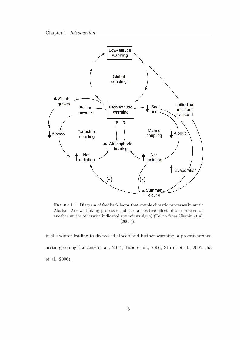
Figure 1.1: Diagram of feedback loops that couple climatic processes in arcticAlaska. Arrows linking processes indicate a positive effect of one process onanother unless otherwise indicated (by minus signs) (Taken from Chapin et al.
(2005)).
in the winter leading to decreased albedo and further warming, a process termed
arctic greening (Loranty et al., 2014; Tape et al., 2006; Sturm et al., 2005; Jia
et al., 2006).
3
Chapter 1. Introduction
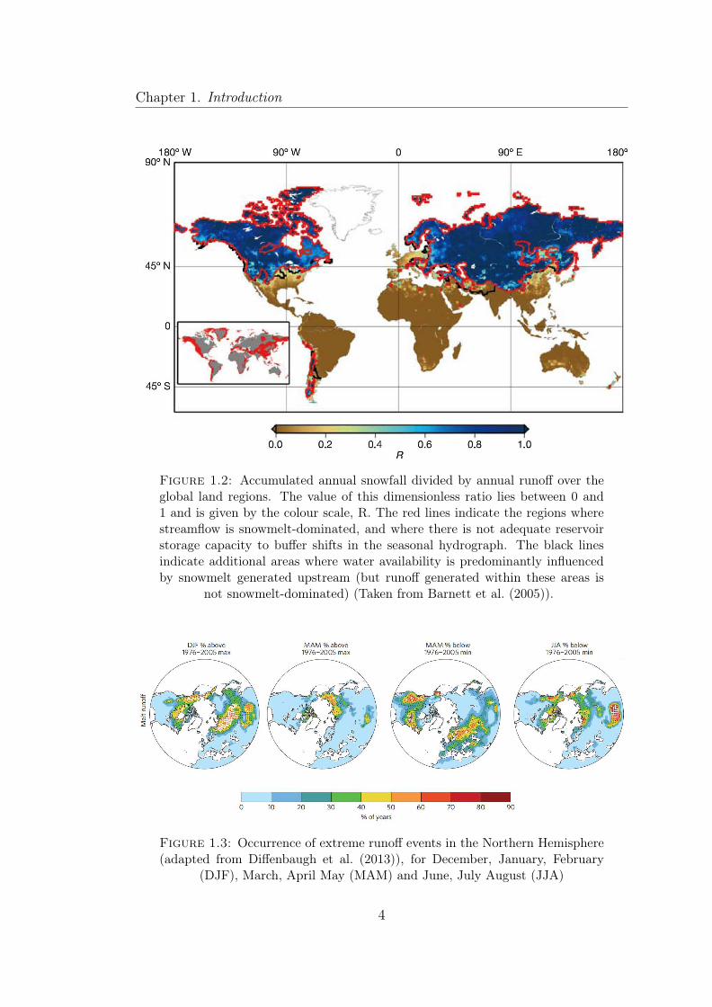
Figure 1.2: Accumulated annual snowfall divided by annual runoff over theglobal land regions. The value of this dimensionless ratio lies between 0 and1 and is given by the colour scale, R. The red lines indicate the regions wherestreamflow is snowmelt-dominated, and where there is not adequate reservoirstorage capacity to buffer shifts in the seasonal hydrograph. The black linesindicate additional areas where water availability is predominantly influencedby snowmelt generated upstream (but runoff generated within these areas is
not snowmelt-dominated) (Taken from Barnett et al. (2005)).
Figure 1.3: Occurrence of extreme runoff events in the Northern Hemisphere(adapted from Diffenbaugh et al. (2013)), for December, January, February
(DJF), March, April May (MAM) and June, July August (JJA)
4

Chapter 1. Introduction
1.2 Measuring Snow Water Equivalent
Snow water equivalent is a function of snow depth and density (Gray and Male,
1981). In situ point measurements of SWE are usually taken using a snow tube.
A snow tube extracts a vertical column of snow from the snowpack which is then
weighed to calculate the SWE of the the snowpack at the given location. The
snow tube allows the key information of depth and density to be recorded more
quickly and in a less destructive manner than a snowpit (Church, 1933; Goodison
et al., 1987; Woo, 1997) and when used as part of a transect provides information
on the spatial variability of SWE.
While a global network of snow weather stations reporting snow depth exists,
station locations are heavily weighted towards populated urban areas (Rees et
al., 2013) and, as a result, are sparse in high latitudes (Brown et al., 2007).
The large size, sparse population and inaccessibility of the Arctic means that
alternative methods need to be used in this region. Model derived hemispheric
estimates of SWE have made significant progress by using reanalysis data to drive
snow and hydrological models and to determine snow accumulation (Troy et al.,
2012; Liston and Hiemstra, 2011). Satellite remote sensing is the most practical
mechanism with which to measure SWE on a hemispheric scale (Vander Jagt et
al., 2013). Near infrared (NIR) and other visible band sensors can be employed to
determine snow extent and other snowpack parameters such a grain size (Painter
et al., 2009). However, visible band measurements have significant drawbacks as
5

Chapter 1. Introduction
they are not able to determine SWE directly and suffer from weaknesses such as
requiring cloud free days and solar illumination, both of which are limitations to
use in the Arctic. Passive microwave remote sensing (Staelin et al., 1977) which,
although it has a course resolution of approximately 25 km (Kelly et al., 2003),
does not require solar illumination, penetrates cloud cover and has a historical
record of > 30 years (Dupont et al., 2012). The 19 - 37 GHz section of the
spectrum is of particular interest for snow remote sensing. At these wavelengths
a snowpack acts to attenuate the microwave emission upwelling from the ground
and the level of attenuation is related to the depth and properties of the snowpack
(Boyarskii and Tikhonov, 2000). The brightness temperature observed by the
satellite radiometer is related to the emission from the earth (which is largely
dependent on its physical temperature) and the attenuation of this emission by
the snowpack (Ulaby et al., 1981).
Extensive work has been carried out to establish theoretical (Grody, 2008; Tse
et al., 2007; Stogryn, 1986) and empirical (Chang et al., 1982; Foster, 1997; Kelly
and Chang, 2003) links between attenuation in the snowpack, observed microwave
brightness temperature and SWE. The classic, empirical approach (Chang et al.,
1982) uses the simple retrieval algorithm
SD = 1.59× (T18H − T37H)cm (1.1)
6

Chapter 1. Introduction
to derive snow depth from brightness temperature, although this has proved to
be unreliable over the Arctic and produced SWE products with large degrees of
uncertainty (Koenig and Forster, 2004; Clifford, 2010).
The majority of the error and uncertainty in SWE products was attributed to
factors such as the forest or lake fraction of the footprint, which are known to
cause variation at the satellite scale (Derksen et al., 2003; Green et al., 2012).
Work focused on quantifying the effect of these factors to improve SWE products,
however, while forest and lake fraction can be observed relatively easily using
existing satellite data products (Derksen, 2008), even when accounting for these
factors uncertainty and error exists in the SWE data products (Foster et al., 2005).
It has been hypothesised (Mätzler, 1994; Boyarskii and Tikhonov, 2000; Durand
et al., 2008; Derksen et al., 2012a) that variation in the properties of the snowpack
and/or our inability to correctly parameterise the variation in snowpack properties
that occur within a satellite footprint using a simple retrieval algorithm, are the
causes of the uncertainty. This has led to an increased interest in both, the
physical properties of the snowpack, and how these properties physically attenuate
the earth’s microwave emission. Sophisticated data assimilation algorithms have
been developed and implemented. Data assimilation organises the useful and
less useful observations into physically consistent estimates of SWE. Ultimately
data assimilation aims to produce the optimal combination of the measurements
where the output (in this case SWE) lies within the error bars of all estimates,
the assimilation estimates will be closer to the more accurate estimates. An
7

Chapter 1. Introduction
example of such an assimilation scheme which uses satellite observations, a land
surface model and a radiative transfer model is shown in Figure 1.4 (Durand and
Margulis, 2007). The approach of Takala et al. (2011) uses in situ measurements
of snow depth in addition to satellite data and an iterative approach to estimate
grain size using a snow emission model to produce a hemispheric product for SWE.
Another approach which has demonstrated improvements in SWE retrievals is to
use a snow model to estimate density and grain size in a coupled snow emission
model (Langlois et al., 2012).
Figure 1.4: This schematic illustrates how the prior information, models,and synthetic measurements are merged using a data assimilation scheme as
described in Durand and Margulis (2007)
8

Chapter 1. Introduction
1.3 Snowpack variability and stratigraphy
Snowpack stratigraphy describes the layered or stratified nature of snowpacks.
Each layer in a snowpack is composed of snow with different properties to the
layers above and below. The variation between snow layers is caused by the suc-
cessive build up of a snowpack by depositional events, and the subsequent impact
of in situ snow metamorphosis, melt, rain-on-snow events or wind compaction
(Colbeck, 1991). Understanding variation in snowpack stratigraphy is crucial for
understanding the microwave emission and radiative transfer properties of snow
(Durand et al., 2008). Snowpack stratigraphy is highly variable at small spatial
scales, although at large spatial scales major stratigraphic units are continuous
(Sturm and Benson, 2004).
Changes in the properties of the snowpack are a key factor in the reflection
and transmission of radiation in the snowpack (Ulaby et al., 1981). Variation
in snowpack stratigraphy is one of the key drivers of variation in modelled and
observed microwave brightness temperatures (Derksen et al., 2012a; Durand et al.,
2008), at scales ranging from the footprint of a ground based radiometer (plot
scale) (Rutter et al., 2014) to the resolution of a satellite derived data product
(Derksen et al., 2012a). Current passive microwave derived SWE products do
not account for spatial variations in snowpack stratigraphy as the ability of
the products to account for snowpack stratigraphy is limited by a lack of field
9

Chapter 1. Introduction
observations. Existing studies that have tried to characterise sub-footprint vari-
ability have focused on either, snow pits taken at a variety of locations within a
satellite footprint (Derksen and Brown, 2012; Elder et al., 2009), or long transects
(Sturm and Benson, 2004). Despite the fact that it is known that variation in
stratigraphy at the sub-footprint to 1 km scale introduces error into estimates of
SWE from brightness temperature measurements (Rutter et al., 2014; Derksen
et al., 2014), it is known that this error does not completely mask the signal
relating brightness temperature to SWE (Vander Jagt et al., 2013; Li et al., 2012;
Derksen et al., 2014). By focusing on the impact of simplifying the stratigraphy
of a given snowpack, it has been found that, at a point, simplification from five
to one layers reduces computational requirements and does not increase error in
simulated brightness temperatures (Huang et al., 2012). However when applied
to field variability, results are more mixed (Rutter et al., 2014; Derksen et al.,
2012a). In addition to this, relatively little has been published looking at small
scale variation in stratigraphy (Rutter et al., 2014; Tape et al., 2010; Derksen,
2008; Pielmeier and Schneebeli, 2003; Sturm and Benson, 2004) and ultimately
the question of whether the variation exhibited at the plot scale can influence
brightness temperatures at the satellite scale is as yet unanswered.
10

Chapter 1. Introduction
1.4 Quantifying variation in snowpack
stratigraphy
Quantifying vertical variation in stratigraphy in a snow pit gives the observer
one profile for that snowpack. Past work has focused on distributing multiple
snow pits around different snow cover types to try to quantify lateral variability
within a satellite footprint (Derksen and Brown, 2012; Derksen et al., 2014).
Other work has utilised a snow trench to quantify stratigraphic variation at cm
resolution over short distances of around 5 m (Rutter et al., 2014; Tape et al.,
2010). The technological development that has enabled this scale of work to
be conducted in situ in a timely manner, is the availability of compact or SLR
cameras adapted to take photos in the near infra-red (NIR) (850 nm) part of the
electromagnetic spectrum. At this wavelength the camera is sensitive to changes
in the microstructure of the snow, and it is possible to use the images to quantify
variability in snowpack stratigraphy over the distance of an excavated snow trench
(Tape et al., 2010; Rutter et al., 2014).
1.5 Aims
The overall goal of this thesis is to improve knowledge of how snowpack stratig-
raphy influences the precision and accuracy of snow microwave emission models
in Arctic tundra environments. This will be achieved by addressing two key
11

Chapter 1. Introduction
weaknesses in our current implementation and parameterisation of snowpack
stratigraphy in snow emission models:
1. The presence of ice lenses and layers in a snowpack substantially increases
bias in horizontally polarised simulated brightness temperatures (Rees et al.,
2010; Durand et al., 2008; Derksen et al., 2012a).
2. The influence of spatial variation of snowpack stratigraphy on brightness
temperature signatures is not well characterised(Derksen et al., 2014).
To help address these weaknesses three aims and associated objectives have been
created
Aim 1: To develop a method that will enable accurate quantification of spatial
variability in snowpack stratigraphy over increased spatial scales on tundra
landcover. To achieve this aim three objectives were identified:
(a) To increase efficiency with which NIR photography of snowpack stratig-
raphy can be collected in the field, and optimise the post-processing
digitisation
(b) to improve accuracy of digitised snow stratigraphy to a consistent 1
cm accuracy across a 5 m snow trench for use in all environments
(c) To Quantify internal snow layer boundary roughness
12

Chapter 1. Introduction
Aim 2: To improve the parameterisation of ice layers in snow emission models
by measuring and analysing the influence of their structural properties
(such as density and bubble size) on the accuracy of simulated brightness
temperatures
(a) To develop a new field method for measuring the density of ice layers
(b) To compare simulated and observed brightness temperatures using
measured ice layer densities to test the sensitivity of the Microwave
Emission Model for Layered Snowpacks (MEMLS) and Multi-layer
Dense Media Radiative Transfer (DMRT-ML) snow emission models
to changes in ice layer parameterisation
(c) To examine the impact that any sensitivity could have on ice layer
detection algorithms
Aim 3: To quantify the variation in stratigraphy within an Arctic watershed, fully
capturing variation in the position of layers and the layer properties.
(a) To quantify layer thickness and boundary roughness variability
(b) To quantify the impact of spatial variability of stratigraphy on Snow
Microwave Emission Models
(c) To determine the minimum subset size in each trench location required
to achieve the mean brightness temperature for that trench
13

Chapter 1. Introduction
1.6 Thesis structure
This thesis will be structured in six chapters, this, the first chapter, serves as the
main introduction, to outline the main motivations, and questions addressed in
this thesis. The second chapter will provide the background to the thesis in more
detail, and provide the context on where this work sits in the current state of
science.
Following these there are three main results and method chapters:
• Chapter 3 introduces the main method of quantifying snowpack stratigraphy
using NIR photography. This method is then used to investigate plot scale,
layer boundary roughness, and intra-layer heterogeneity for two sites in the
sub arctic.
• Chapter 4 will address the parameterisation of ice layers, and introduce a
specific method which was implemented to carry out this work.
• Chapter 5 will use the methods outlined in chapter 3, but on a larger
scale, to investigate variation in snowpack stratigraphy and simulations from
emission models over different landcover types in an Arctic drainage basin.
The final chapter, chapter 6, acts as a synopsis to summarise and discuss the
overall findings of the thesis and outline future work.
14

Chapter 2
Origins of microwave signatures in
tundra snowpacks
2.1 In situ quantification methods of natural snow
cover
Snow pack stratigraphy provides important information about the properties,
processes and dynamics of a snowpack, it has numerous uses in snow hydrology,
avalanche prediction and, as explored in more detail in this Chapter, snow remote
sensing. In situ measurements of snowpack stratigraphy are typically made by
opening up a snow pit face and recording information as a profile down the wall
of the pit, although as will be discussed in section 2.1.3 some newer technologies
provide alternatives.
15

Chapter 2. Origins of microwave signatures in tundra snowpacks
2.1.1 Snow pit measurements
The first measurement made in a snow pit is the overall depth of the snowpack
and then its layered structure, typically a vertical resolution of 1 cm is used to
achieve this. Textural information about the snowpack is recorded, including
its hardness. This one dimensional method of recording snow pack stratigraphy
makes the assumption of discrete boundaries between layers, and that snow layers
are parallel (Pielmeier and Schneebeli, 2003). Snow temperature is typically
recorded at set intervals through the snowpack.
Snow density is the bulk snow mass per unit volume. Classically it is measured
by weighing a snow sample of known volume. A snow sample of known volume
is extracted from the snow pit face using a wedge or square snow density cutter.
Measurements are made either as a continuous profile down the pit face, at set
intervals or using one sample per identified layer. It is also possible to measure
density using the snow’s dielectric properties (Mätzler, 1996).
Snow grain type changes as the snow is metamorphosed on the ground. Grain
shape is classified in Fierz et al. (2009). The type (or types) of crystals in a
layer are identified in the field using a magnifying glass or field microscope and
a crystal card. Grain size is measured in the same manner, grain size is the
most common metric used to quantify snow microstructure although newer less
subjective methods are emerging, as discussed in Section 2.1.3.
16

Chapter 2. Origins of microwave signatures in tundra snowpacks
2.1.2 Measuring spatial variability
Snow variability has historically been recorded using a snow course (Gray and
Male, 1981). A snow course consists of a well defined path or track that is
routinely sampled along over a period of time. The snow course aims to cover as
many different land cover and topography types as possible within the practical
limitations of a single survey. Snow pits and dug, and bulk density measurements
and snow depth measurements are taken along the snow course. Snow courses
allow spatial (and with repeat sampling, temporal) snowpack variability to be
measured although they do not provide continuous snow stratigraphy information
as some emerging technologies can (Section 2.1.3).
2.1.3 Emerging Methods
Emerging methods and technologies are providing new methods with which to
measure snow pack stratigraphy at a single profile, these improve methods of
measuring the specific surface area (SSA) of snow. SSA is physically important
as it directly relates the the way in which snow interacts with optical radiation
and is therefore a good way to quantify snow microstructure. Several methods
exist for measuring SSA including using the reflectance from a 1310 nm laser
(Gallet et al., 2009) and near infra-red photography (described in more detail in
section 2.1.4). Additionally it is also possible to measure the microstructure of
snow directly by utilising a microCT scanner (Heggli et al., 2009).
17

Chapter 2. Origins of microwave signatures in tundra snowpacks
2.1.4 NIR Photography
The NIR part of the spectrum is sensitive to changes in the SSA of snow (Matzl
and Schneebeli, 2006). Using this physical property NIR photography has been
utilised to capture the structure of a snowpack in the field. Tape et al. (2010)
developed a method to identify and quantify snowpack stratigraphy using near
infra-red (NIR) photography. A Fuji S9100 digital camera was adapted to be
sensitive to light with mid-point wavelength of 850nm and by photographing
the side of a snow trench at 50cm horizontal intervals, the stratigraphy of the
snowpack became more apparent and could be quantified digitally from the pho-
tographs (Matzl and Schneebeli, 2006). It is possible to use the images to quantify
variability in snowpack stratigraphy over the length of the trench (Rutter et al.,
2014).
Using NIR photography along a trench provides considerable advantages and
speed increases over recording stratigraphy with manual inspection in the field
(Tape et al., 2010). However, there are two major weaknesses with this technique.
Firstly, the processing time required to extract digitised stratigraphy from the
images can be extensive. Using previous methodologies and protocols one 5 m
trench could take up to a day. Secondly, variation in the focal length of the
camera causes changes in scale along the trench which introduces error. In Tape
et al. (2010) trenches were excavated on a frozen lake, this helped minimise
uncertainty in this area allowing for the method to be developed in a somewhat
18

Chapter 2. Origins of microwave signatures in tundra snowpacks
idealised environment with very little topographic variation. When the method is
applied to environments with more varied subnivean topography the uncertainty
between the digitised snow layers and geo-referenced trench position increases,
and a more rigorous method for translating a point location is required. This
makes assigning measurements taken in the field to a specific snow layer difficult.
Past work has approached the problem by utilising a strict protocol to, while
not eliminate, hopefully constrain uncertainty (Rutter et al., 2014). In this work,
overall average values were applied to each layer in the snowpack, so any variation
in snow properties that occurred within a layer, in the scale of the trench, was
not accounted for, characterised or quantified.
NIR photography of a snow trench provides high resolution surface and layer
boundary roughness (the roughness between the snow layers within a snowpack)
information. Surface roughness is a control on the transfer of wind energy, and
affects snow transport, redistribution and latent and sensible heat exchanges
(Fassnacht et al., 2009b). Information at a resolution high enough to constrain
layer boundary roughness cannot be obtained from in situ field measurements
alone, as the time required is too great. In the past, surface roughness has
been characterised over small distances and over larger scales (Fassnacht et al.,
2009a) although roughness between snow layers has never to my knowledge been
measured or characterised. Theoretically layer boundary roughness has a large
impact on radar backscatter (Marshall and Koh, 2008), although it has never
been quantified at the plot scale.
19

Chapter 2. Origins of microwave signatures in tundra snowpacks
2.2 General Principles of Passive microwave
remote sensing
Kirchhoff’s law of thermal radiation (1860) states that when an object is at
thermal equilibrium (neither warming nor cooling) then the power radiated by
the object must be equal to the power absorbed. An object that absorbs and
reradiates 100% of the radiation incident upon it is described as a blackbody, an
object that absorbs (and therefore reradiates) less than 100% is described as a
grey body. The spectral radiance of a blackbody (B) at a particular frequency (v)
is dependent only on the blackbody’s physical temperature, and can be calculated
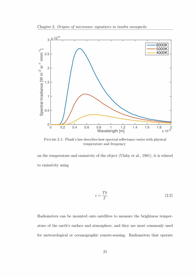
using the Plank Radiation Law as shown in Equation 2.1 and Figure 2.1 where
kB is the Boltzmann constant, h is the Plank constant, and c is the speed of light.
B(v, T ) =2hv3
c21
ehvkBT − 1
(2.1)
Emissivity, ϵ, is a measure of the efficiency with which a surface emits thermal
energy. It is the brightness of a grey body relative to a black body of the same
temperature (for a blackbody ϵ = 1) (Ulaby et al., 1981). Brightness temperature
is the quantity measured by a radiometer and describes the intensity of radiation
emitted by an object or area under observation. Brightness temperature depends
20
Chapter 2. Origins of microwave signatures in tundra snowpacks
Wavelength [m] -60 0.2 0.4 0.6 0.8 1 1.2 1.4 1.6 1.8 2
Spec
tral I
rradi
ance
[W m
-2 s
r-1 n
mm
-1]
x 1014
0
0.5
1
1.5
2
2.5
36000K5000K4000K
x 10
Figure 2.1: Plank’s law describes how spectral reflectance varies with physicaltemperature and frequency
on the temperature and emissivity of the object (Ulaby et al., 1981), it is related
to emissivity using
ϵ =Tb
T. (2.2)
Radiometers can be mounted onto satellites to measure the brightness temper-
ature of the earth’s surface and atmosphere, and they are most commonly used
for meteorological or oceanographic remote-sensing. Radiometers that operate
21

Chapter 2. Origins of microwave signatures in tundra snowpacks
at frequencies suitable for snow remote sensing and are currently in orbit (both
working and non-working) are listed in Table 2.1.
Table 2.1: Passive Microwave satellite radiometer missions suitable for snowremote sensing
Instrument Mission AvailabilitySMMR Nimbus 1978-1987SSM/I DMSP 1987-SSMIS DMSP 2003-AMSR ADEOS-II 2002-AMSR-E EOS Aqua 2002-2011AMSR2 GCOM-W 2012-PRIRODA MIR 1996-2001
2.3 Snow emission modelling
The ability to simulate snow microwave emission is useful both for use in data
assimilation and SWE retrieval schemes, and to better enable us to understand the
radiative properties and processes of snow and ice. The simulation of microwave
brightness temperatures of a snowpack is approached in two parts. Firstly the
electromagetic properties (effective dielectric constant, scattering and absorption
coefficients) that characterise the interaction between the wave and snow are
calculated from the microstructural properties of the snow. Secondly the emission
and propagation through the snowpack are calculated by accounting for the inter-
actions within the snow as well as the refraction, reflection and transmission that
occur at interfaces between snow layers or between the snow and the air/ground.
22

Chapter 2. Origins of microwave signatures in tundra snowpacks
Several models exist to solve these problems. In this thesis, n-HUT (Lemmetyinen
et al., 2010), MEMLS (Wiesmann and Mätzler, 1999) and DMRT-ML (Picard
et al., 2013) are used. Tedesco and Kim (2006) compared simulations from a large
number of snowtypes and demonstrated that no particular model systematically
reproduces all of the experimental data. They were unable to attribute their
discrepancies to any root cause, so it is not known if problems are attributable
to the fundamental electromagnetic theory, specific details of the models, or if
there was uncertainty in the evaluation data, and the methods used to represent
snow grain size. Snow emission models are currently not able to accurately
and consistently reproduce observed Tb values without using additional scaling
factors and coefficients to tune model output (Derksen et al., 2012a; Langlois
et al., 2012; Rutter et al., 2014). Three areas have been identified as the primary
source of bias in simulations: the quantification and parameterisation of observed
snow microstructure in model input (Langlois et al., 2010); uncertainty in the
simulation of emission from the ground and soil under the snowpack (Roy et al.,
2013); and the inability of models to take full account of snowpack stratigraphy
including the presence of ice layers (Durand et al., 2011).
23

Chapter 2. Origins of microwave signatures in tundra snowpacks
2.4 Passive microwave remote sensing of snow
2.4.1 Principle
For a snow covered land surface, the brightness temperature observed by a space
borne radiometer is affected by:
1. Soil
• Physical temperature
• Soil dielectric profile
• Surface roughness
• Textural composition
• Volume scattering within the soil
2. Vegetation
• Absorption and emission determined by physical temperature, mois-
ture and physical characteristics of the plants
• Volume scattering within the vegetation, and surface scattering at
vegetation interfaces, determined by physical structure of plants
3. Atmosphere
• Weather conditions effect the scattering and absorption in the atmo-
sphere
24

Chapter 2. Origins of microwave signatures in tundra snowpacks
• Cosmic microwave background emission
4. Snowcover
• Scattering properties of snow cover, determined by snow microstruc-
ture
• Absorption and emission of snow, determined by snow density, tem-
perature and wetness of the snowpack
• Total mass of snow in the propagation path of microwaves, given by
the snow water equivalent
There is a theoretical relationship between the SWE of a snowpack and its
observed brightness temperature. Defining this relationship is complicated by
the fact that the emission from and attenuation by the snowpack depend on
many factors in addition to SWE
2.4.2 Retrieval Algorithms
Passive microwave data is of particular use for the creation of global snow products
as it has a large spatial extent, frequent revisit times (up to twice daily) and
relatively long term temporal continually (Tait, 1998). For this reason, a great
deal of research has focused on developing and improving methods of retrieving
SWE from passive microwave brightness temperatures (Chang et al., 1981; Foster
et al., 1980; Goodison and Walker, 1995; Pulliainen and Hallikainen, 2001; Tait,
25

Chapter 2. Origins of microwave signatures in tundra snowpacks
1998; Hallikainen and Jolma, 1992; Grody and Basist, 1996). The following
sections will describe the different types of algorithm and approach that have
been taken to solve this problem, starting from simple empirical algorithms, to
modified, landscape-specific empirical algorithms, and then finally model based
approaches.
2.4.2.1 Empirical
The classic approach for the calculating SWE using passive microwave brightness
temperature compares the brightness temperature of a frequency expected to be
readily scattered and absorbed by the snow cover and the brightness temperature
of a frequency that will not experience so much scattering. An empirical rela-
tionship can be established between the differences in brightness temperature
of the two frequencies and the SWE of the snowpack. Foster et al. (1980)
identified 37 GHz as a frequency which is sensitive to the snowpack and 19
GHz as having a wavelength long enough to not be affected by the snow cover
but rather the underlying soil. Figure 2.2 shows the effect of grain size on 37
GHz (vertically polarised) brightness temperature. As grain size approaches the
wavelength of a specific frequency, scattering at that frequency will increase.
Brightness temperatures for 37 GHz are therefore affected by snow microstructure
and grainsize in addition to snow water equivalent.
The first hemispheric algorithm to describe such a relationship was the Chang
algorithm (Chang et al., 1987), shown in Equation 2.3 where SD is snow depth.
26

Chapter 2. Origins of microwave signatures in tundra snowpacks
Figure 2.2: Effect of Grain Size on 37 GHz, vertical polarisation brightnesstemperature (Adapted from Rees (2006) redrawn from data presented in
Armstrong et al. (1993) and Chang et al. (1981)
By assuming a snow density of 300 kg m−3 this algorithm was used to calculate
SWE at a hemispheric scale.
SD = 1.59× (T18H − T37H)cm (2.3)
2.4.2.2 Modified Empirical
At a global scale problems arise where, within one satellite footprint, multiple
landcover types need to be integrated across in order to provide continuous and
standardised spatial coverage. In order to address these problems, successive
27

Chapter 2. Origins of microwave signatures in tundra snowpacks
retrieval algorithms have worked to subset landcover types and incorporate addi-
tional parameters specific to them. The Meteorological Service of Canada (MSC)
(now part of Environment Canada (EC)) developed algorithms for a wide range
of Canadian landcover types, all based around the form
SD = a− b× (T37V − T18V ) (2.4)
where SWE is snow water equivalent in mm and a and b are empirical parameters.
For example Walker and Silis (2002) assign a = −20.7, b = 2.59 for use in the
lake scattered tundra of the Mackenzie River basin. These and other similar
algorithms have been used operationally since 1988 and have been shown to be
accurate to ±10 − 20 mm SWE (Derksen et al., 2002; Goodison and Walker,
1995). A similar approach has been used on SMMR data which has allowed for
a longer time series to be created (Derksen et al., 2003).
When a snowpack reaches a certain depth, the saturation of microwave radiation
occurs (Sturm et al., 1993), this is when all of the emission from the earth
is absorbed by the snowpack (Kelly et al., 2003). The depth of snow where
saturation occurs is different for every frequency (Durand and Margulis, 2006).
The depth that radiation is able to penetrate into the snowpack is called the
penetration depth. The penetration depth changes with frequency and grainsize
as is shown in Figure 2.3. The shorter penetration depth of higher frequencies
28

Chapter 2. Origins of microwave signatures in tundra snowpacks
has the potential to be useful as it allows information to be gained about specific
parts of the snowpack, for instance, 37 GHz has a penetration of around 35 cm,
this provides a penetration depth similar to the depth of a tundra snowpack
and so, changes in shallow snowpacks are particularly detectable at 37 GHz.
For a frequency around 89 GHz only the surface of the snow at the snow-air
interface impacts the signal, so changes in this part are of particular importance
to brightness temperature changes at this frequency.
Figure 2.3: Variation in penetration depth between different frequencies(Adapted from Ulaby et al. (1986))
in addition to the MSC, Tait (1998) produced a SWE product by dividing the
northern hemisphere into different vegetation and open landcover types, however,
confidence in the results were low, with depth hoar development (discussed more
in 2.5.3), high wind distribution (discussed in section 2.5.4) and boreal forest
proved problematic for the algorithms.
29

Chapter 2. Origins of microwave signatures in tundra snowpacks
2.4.2.3 Model based
While using different algorithms for different land cover types goes some way
towards addressing the issue of spatial heterogeneity between landcover types,
it does not begin to address issue of to how the snowpack changes temporally.
More recently work has looked to develop algorithms based on those of Chang
et al. (1987) that also account for seasonal evolution (Kelly and Chang, 2003),
snow metamorphism (see also section 2.5.3) (Josberger and Mognard, 2002) and
topography (Kelly et al., 2003).
The HUT model inversion method used by Pulliainen and Hallikainen (2001)
iterates the HUT snow microwave emission model to minimise the difference
between modelled and observed brightness temperatures. This is achieved by
optimising the values for SWE and grain size. The algorithm also accounts for
forest fraction in a satellite footprint.
As there are inherent weaknesses with all remote sensing, modelled and observed
SWE data products, current work is highly focused on using a combination of
multiple methods for deriving SWE in a data assimilation scheme (Takala et al.,
2011; Durand et al., 2011). A data assimilation algorithm takes the estimated
values from several sources, and by combining them, and accounting for their
errors (assuming error and uncertainty are known) a more accurate value can be
calculated. There are many different methods which can be utilised within the
field of data assimilation involving the implementation of a variety of different cost
30

Chapter 2. Origins of microwave signatures in tundra snowpacks
functions and algorithms. Generally a mixture of remote sensing and modelled
data is used in order to provide the full scope of possible values (Reichle, 2008).
For SWE data assimilation schemes snow emission models are a key component,
as they provide a modelled value for remotely sensing brightness temperatures
and can be iterated in certain schemes to calculate parameters which are required
in other models or data products.
2.5 Challenges in the application of retrieval
algorithms
Despite the wide range of research which has been carried out into the use of
conventional retrieval algorithms to derive SWE, it is widely accepted that no
consistently accurate SWE or snow depth product has resulted. In tundra snow-
packs, conventional retrieval algorithms result in a consistent underestimation of
SWE compared to in situ ground measurements (Grippa et al., 2004; Armstrong
and Brodzik, 2002). The reason for the uncertainty can be attributed to an
inability of these algorithms to account for heterogeneity in the snowpack and
snowpack properties within a satellite footprint (Derksen et al., 2012a). This
section will now review the causes of the heterogeneity and the impact that has
been attributed to each aspect.
31

Chapter 2. Origins of microwave signatures in tundra snowpacks
2.5.1 Layering
In the Arctic, seasonal snow layers form within the snowpack. Sturm et al. (1995)
stated that a typical tundra snowpack consists of 6 layers, the least of any snow
cover class with the exception of very thin ephemeral and prairie snow cover.
A typical Arctic or sub-arctic snowpack is composed of a depth hoar layer at
the base of the snowpack. Over that are several high density wind slab layers
and then a top layer of freshly deposited (either by wind or precipitation) snow
(Derksen et al., 2014). The structure of the snowpack has been identified as an
important component in determining the brightness temperature of a snowpack.
Snowpack structure has been recognised as being particularly difficult to interpret
and quantify in the spectral signature of snow cover (Bernier, 1987).
When characterising stratigraphy a tundra snowpack can generally be simplified
into three main snow types (Sturm et al., 1993). The bottom of the snowpack is
composed of large grained depth hoar, the volume of depth hoar is of particular
importance for passive microwave remote sensing (Foster et al., 1999; Foster et al.,
2000). The second type is composed of higher density smaller grain size wind slab
layers. These layers, formed by the successive wind re-distribution and overlaying
of precipitated snow (Derksen et al., 2014) can also include indurated depth
hoar (Sturm et al., 1993), where depth hoar faceting has developed within the
wind slab. The hardnesses will vary between layers, however, due to the similar
wind based method of compaction the grain diameter is often similar and small.
32

Chapter 2. Origins of microwave signatures in tundra snowpacks
The top layer is composed of fresh, recently precipitated snow and generally
comparatively thin compared to the other two layers. This layer is thin because
of the wind redistribution of snow in tundra environments, in forest or shrub
dominated landscapes, where wind speed is lower, this top layer is likely to be
thicker.
2.5.2 Variability in Stratigraphy
Our ability to quantify variability in snowpack stratigraphy is limited by a lack
of field measurement. The reasoning for this is that measuring and recording
snowpack stratigraphy information requires specific skills and can be laborious
and time consuming (Sturm and Benson, 2004). A snow pit provides only one
snow profile at one location and so generating statistically significant distributions
of snowpack variability is challenging. The majority of existing studies focus on
either snow pits taken at a variety of locations within a satellite footprint (Derksen
and Brown, 2012; Elder et al., 2009) or along transects at scales ranging from
hundreds of metres to thousands of km (Sturm and Benson, 2004) in order to
try to capture the variability within one, or multiple landcover types. Despite
the fact that variation in snowpack stratigraphy at the plot scale introduces error
into estimates of SWE from brightness temperature measurements (Rutter et al.,
2014), at larger scales there is still a significant relationship between brightness
temperature to SWE and (Vander Jagt et al., 2013; Li et al., 2012). Work has
focused on the impact of simplifying the stratigraphy of a given snowpack, and
33

Chapter 2. Origins of microwave signatures in tundra snowpacks
has found that some simplification reduces computational requirements and does
not increase error in simulated brightness temperatures (Huang et al., 2012).
However, these studies have only been based on a small number of profiles of
snowpack stratigraphy distributed over a surface. While they exhibit a large and
concerted effort to cover different land cover and terrain types, there are still
questions over whether a network of snow pits can capture the range of snowpack
stratigraphy, and there is a gap in the literature examining whether a single
snowpack profile obtained from a snow pit can characterise the snowcover for one
landcover type.
Snow layers vary in thickness at different scales (Sturm and Benson, 2004) but
additionally, smaller scale roughness between the boundaries of the snow layers
can be characterised using roughness metrics (Fassnacht et al., 2009b; Anttila
et al., 2014), although these have previously only been applied to snow surface and
ground roughness. Currently, snow emission models simulate brightness tempera-
ture in one dimension. However, as the science progresses so that two dimensions
are used, a roughness will need to be applied to the layer boundaries. Currently,
the internal roughness of layer boundaries is not known. An additional use of this
layer boundary roughness information is its application in nadir FMCW sensors,
where the layer boundary roughness contributes greatly to the attenuation of the
snowpack (Marshall and Koh, 2008).
34

Chapter 2. Origins of microwave signatures in tundra snowpacks
2.5.3 Depth Hoar
Volume scattering within the snowpack is directly influenced by the grain size of
the snow crystals in the snowpack. It is therefore an extremely important and
sensitive parameter in passive microwave snow remote sensing (Hall et al., 1986).
When depth hoar is present in the snowpack the grain size can approach or exceed
the wavelength being measured, this causes the lower than expected brightness
temperature values(Hall et al., 1986). The effect of this increased scattering is
so pronounced that, once a depth of just 30cm of depth hoar is reached, all of
the radiation emitted by the earth at 37 GHz is scattered and the brightness
temperature is composed of the emission from the mass of the snowpack alone
(Sturm et al., 1993). In addition to the grain size, the shape of the crystals also has
an impact (Foster et al., 2000; Foster et al., 1999). As the depth hoar grows in the
snowpack brightness temperatures will drop due to increased scatter. However,
SWE may well remain the same. Accounting for this is a key consideration in
the use of retrieval algorithms for tundra snow. However, work by Koenig and
Forster (2004) showed that it is possible to achieve consistently accurate SWE
estimates in depth hoar dominated snow as long as the data is temporally and
spatially averaged over multiple footprints.
35

Chapter 2. Origins of microwave signatures in tundra snowpacks
2.5.4 Wind re-distribution
Snow cover is precipitated and then redistributed by the action of wind transport.
Large scale wind transport does occur and is controlled mainly by large climatic
and geographic features such as lake effects, mountain ranges etc. (Pomeroy
and Gray, 1995). While this is important for global and hemispheric modelling
applications it is not necessary to account for this in passive microwave remote
sensing as it occurs at a much larger scale than the spatial resolution of the
satellite sensors.
The aspect of wind distribution which is most important when addressing weak-
nesses in passive microwave remote sensing is the redistribution effects that occur
at a spatial scale within one land cover - specifically within one satellite pixel
( < 25 km). It is not currently known exactly what impact small scale changes in
snowpack stratigraphy (the most immediate impact of wind re-distributed snow)
has on satellite scale brightness temperatures. This question can be considered
a sub-question of the larger pressing question of the impact of snowpack hetero-
geneity within a satellite footprint, one which is starting to be addressed (Derksen
et al., 2012a).
2.5.5 Melt and rain-on-snow events
Ice structures form in snowpacks during melt or rain-on-snow events (Colbeck,
1991), when rain either freezes on contact with the surface of the snowpack or
36

Chapter 2. Origins of microwave signatures in tundra snowpacks
water refreezes within the snowpack to form ice layers, ice columns, or basal
ice layers (Gray and Male, 1981). Strong intercrystalline bonds, created from
refreezing of liquid water, lead to the formation of cohesive ice structures (Fierz
et al., 2009). The presence of ice layers changes the thermal and vapour transport
properties of the snowpack (Putkonen and Roe, 2003). Permeability of ice layers
to liquid water and gas is vastly reduced compared to snow(Albert and Perron
Jr, 2000; Colbeck and Anderson, 1982; Keegan et al., 2014). Impermeable layers
are identifiable because pores do not connect within the ice formation and the
granular snowpack structure is missing (Fierz et al., 2009). Ice layers differ from
ice crusts and lenses; ice crusts are always permeable and have a coarse grained
granular snow-like structure (Colbeck and Anderson, 1982). Ice lenses are similar
to ice layers in that they can be impermeable and do not have a granular structure,
but ice lenses are discontinuous ice bodies that cover much smaller spatial scales
than ice layers (Fierz et al., 2009).
Ice layers (the focus of Chapter 4) introduce uncertainty into the performance of
microwave snow emission models when simulating horizontal polarisations (Rees
et al., 2010). Snow emission models are an important component of satellite
derived snow water equivalent (SWE) retrieval algorithms, and existing algo-
rithms favour using vertically polarised brightness temperatures over horizontal
primarily to avoid the issues with ice layers (Takala et al., 2011). The radiometric
influence of thin ice layers poses a significant challenge for physical and semi-
empirical emission models, which have either focused on modelling ice crusts as
37
Chapter 2. Origins of microwave signatures in tundra snowpacks
coarse grained snow (Matzler and Wiesmann, 1999) or as planar (flat, smooth
and solid) ice layers (Lemmetyinen et al., 2010). The structure and properties
of ice layers remain poorly quantified with field observations (Montpetit et al.,
2012), which further hinders model development and evaluation. Improving snow
emission models to include more realistic simulations of ice layers by accounting
for ice layer density should improve model estimates of brightness temperatures
(Durand et al., 2008; Montpetit et al., 2012; Rutter et al., 2014).
Field measurements of ice lens, crust and layer densities exist, however, they vary
drastically and a quantitative assessment of the error in measurement techniques
is absent. Ice crust density measurements taken in the Canadian Arctic by
submerging pieces of ice crust into oil resulted in a range of densities from 630
to 950 kg m−3 (Marsh, 1984) and ice layer densities of 400 to 800 kg m−3 were
measured in seasonal snow on the Greenland ice sheet (Pfeffer and Humphrey,
1996). Durand et al. (2008) carried out sensitivity studies and simulations of
mountain snowpack brightness temperature with MEMLS (Wiesmann and Mät-
zler, 1999). The uncertainties attributed to not knowing the density of ice
layers were 32.2 K and 15.3 K, for horizontally polarised (H-pol) 18.7 GHz and
36.5 GHz frequencies respectively. This was a greater uncertainty than any other
parameter investigated (Durand et al., 2008). An increase in the number of mid-
season melt and rain-on-snow events in a warming climate is likely to increase the
occurrence of ice layers and the importance of accurate ice layer representation
in snow emission models (Derksen et al., 2012a).
38

Chapter 3
Digitising Snowpack Stratigraphy
with Improved Accuracy
3.1 Research aims and objectives
Based on the gaps in the literature described in Chapter 1, four problems have
been identified. The problems will be solved by achieving their associated research
aim and objectives as outlined below:
• Problem 1:
Using NIR photography to digitise stratigraphy is too time consuming to
be useful at a large spatial or temporal scale
39

Chapter 3. Digitising Snowpack Stratigraphy
• Aim:
To increase efficiency with which NIR photography can be collected in the
field and optimise post-processing digitisation procedure
– Objective 1: To find alternatives to, or negate the need for, the more
time consuming aspects of field methods
– Objective 2: To automate aspects of the post processing procedure to
reduce time required for digitisation
• Problem 2:
It is not possible to assign in situ snowpack measurements to digitised layer
positions on uneven terrain without subjective human input
• Aim:
To improve accuracy of digitised snow stratigraphy across a 5 m snow trench
for use in all environments
– Objective 1: To adapt existing field method to better record informa-
tion of scale
– Objective 2: To account for the variation in scale within the trench in
post processing
– Objective 3: To develop an automated approach for assigning snow
properties to snow layers based on the location of the measurement in
the trench, and the location of the digitised snow layer
40

Chapter 3. Digitising Snowpack Stratigraphy
• Problem 3:
The impact of variability within snow layers on brightness temperature
simulations from snow emission models at the plot scale is unknown
• Aim:
To characterise variability within snow layers along a 5 m trench, and de-
termine the impact of this variability on simulated brightness temperatures
from the n-layer Helsinki University of Technology snow emission model
(n-HUT)
– Objective 1: To use automated technique from Aim 2 to assign snow
properties to layers and characterise variability in snow layer properties
across the snowpack
– Objective 2: To run n-HUT snow emission model at all points along
5 m trenches
• Problem 4:
Roughness of snow layers within the snowpack is unknown, yet is theoreti-
cally a very sensitive parameter for snow emission models
• Aim:
To quantify internal snow layer boundary roughness
– Objective 1: To use the more accurate digitised snowpack stratigraphy
from Aim 2 to calculate roughness metrics for snow layer boundary
roughness
41

Chapter 3. Digitising Snowpack Stratigraphy
– Objective 2: To characterise and quantify variation in snow layer
boundary roughness within and between different snowpacks
3.2 Development of stratigraphy digitisation
method
Tape et al. (2010) developed a method to identify and quantify snowpack stratig-
raphy using near infra-red (NIR) photography. By adapting a Fuji S9100 digital
camera to be sensitive to light with mid-point wavelength of 850nm and pho-
tographing the side of a snow trench at 50 cm horizontal intervals, the stratigraphy
of the snowpack became more apparent and could be quantified digitally from
the photographs (Matzl and Schneebeli, 2006). In the field, snowpack properties
were recorded for each snow layer along the trench. This section presents a
series of optimisations and improvements which have been made to the initial
methodology from Tape et al. (2010). They both, improve the ease with which
snow stratigraphy data can be collected from the NIR photography, and offer
improvements in the accuracy and precision of that data addressing Aims 1 and
2 in the previous section.
42

Chapter 3. Digitising Snowpack Stratigraphy
3.2.1 Preparing the NIR images
The techniques described here can be applied to any NIR images which are
obtained using a field methodology similar to that described in Tape et al. (2010).
All the examples are taken from fieldwork carried out at Churchill MB, Canada
in the winter of 2010/2011 (described in Section 3.3). The trench images contain
horizontal and vertical points of reference, a horizontal measuring staff which
covers the entire length of the trench and a vertical metre rule or additional
measuring staff which is positioned on the trench for each photo (Figure 3.1).
Each trench is 5 m long and covered by 10 individual images, taken at 50 cm
intervals.
Figure 3.1: An example of NIR snow trench photography
The images were stitched into one large image covering the entire trench, however,
before this, they needed to be corrected for lens barrel distortion. In past work the
commercial software PTgui has been used to carry out this correction (Tape et al.,
43

Chapter 3. Digitising Snowpack Stratigraphy
2010). Here the open source alternative Hugin (Hugin 2011) is used as it offered
better scripting capabilities for processing a high volume of images. Figure 3.2
shows the final stitched NIR image from this process that is now suitable for layer
identification and digitisation. The example trench is the first trench collected
on an open tundra site at Churchill MB in 2012, this is described in section 3.3.
Figure 3.2: NIR images stitched together to show stratigraphy across trench
3.2.2 Extracting snow stratigraphy information from NIR
snow trench photography
Previously the pixel locations of the layers in the snowpack were recorded one by
one to record the snowpack stratigraphy. This was a time consuming and labo-
rious process, which made editing the location of the snow layers and correcting
any mistakes difficult and time consuming.
Snowpack digitisation was made more efficient by recording the location of the
snow layers in the snowpack using Adobe Illustrator image processing software.
Two layers were used in the software, one containing the images from the NIR
photography and a second containing the stratigraphy of the snow. Each layer
identified in the snowpack was drawn in a different colour over the image and
once all the layers had been drawn the layer containing the NIR photography
44

Chapter 3. Digitising Snowpack Stratigraphy
was turned off, leaving an image the same size as the NIR photography, but
only containing the digitised snow layers. The layer locations (in pixels) were
extracted from the image using the Image Processing Toolbox in MATLAB, and
the different layers identified and separated using their RGB values. The output
from this process for the example trench is shown in figure 3.3.
Figure 3.3: Position of digitalized snow layers in pixels, i.e. before pixellocations have been translated into geo-referenced cm co-ordinates
Snow and radiative transfer models require snowpack snow layer heights that are
parameterised in cm. By measuring the graduations on the horizontal and vertical
measuring devices it is possible to convert a pixel × pixel co-ordinate read from
the image in MATLAB into a cm × cm co-ordinate.
45

Chapter 3. Digitising Snowpack Stratigraphy
3.2.3 Calculating positions in digital images in cm
In Tape et al. (2010) and Rutter et al. (2014) a manual graduation size quan-
tification method is used. The location of graduations and the number of pixels
between them can be quantified using the Matlab image processing toolbox which
records the locations of points located with a cursor on the image. Here the
horizontal pixel per cm values were measured using a more automated method,
which completely removes the element of human error from the process and also
decreases the time taken by a factor of approximately ten.
To measure the graduations a GUI has been developed where a line is drawn over
the graduations of the staff (Figure 3.4) and the distance between every edge under
that line measured automatically. From this, the number of pixels between each
graduation can be determined as well as their exact location on the image. To do
this the Canny edge detection algorithm (Canny, 1986) is applied to the image, as
shown in Figure 3.4b. The Canny algorithm works by applying a Gaussian filter
to the image and the regions of the image with a high spatial derivative are then
highlighted to create a gradient magnitude image. Edges are determined by the
location of ridges in the gradient magnitude image, the algorithm tracks along
the ridges setting all other values to zero thereby defining the image edges. Two
threshold values, T1 and T2, are set as parameters where T1>T2. Tracking can
only start at a location on a ridge where the pixel brightness value, or ridge height
is greater than T1, and continues out from the starting point in all directions until
46

Chapter 3. Digitising Snowpack Stratigraphy
the ridge height is less than T2 (Canny, 1986). The parameters are set to identify
the outline of the graduations on the measuring staff. Noise, identified as edges
less than 10 pixels in length, is then removed from the image. When a line is
drawn over these detected edges using a GUI, the pixel co-ordinates of the points
underneath that line are checked against the binary edge image created by the
Canny algorithm. By doing this the position of edges can be detected. After the
locations have been recorded, any errors (such as areas where the graduations are
obscured) are removed manually from the data.
(a) Measuring staff prior to apply-ing edge detection
(b) Measuring staff after applyingedge detection algorithm
(c) GUI for quantifying size of cm graduations in pixels
Figure 3.4: The impact of applying the canny edge detection algorithm to ameasuring staff to assist in determining the pixel per cm ratio across a snow
trench
To convert the pixels per graduation into a geo-referenced location efficiently the
variation in pixel per cm values across the image are converted into a translation
47

Chapter 3. Digitising Snowpack Stratigraphy
matrix (T). T is the same size as the stitched image, where each cell contains
a decimal value which, when divided by the pixel co-ordinates of that location,
returns that same location as a geo-referenced cm by cm x, y co-ordinate. The
purpose of this is to allow snow layer boundaries to be identified on the stitched
trench image and then quickly converted into a format for use in mathematical
models or in the measurement of roughness. Once T has been created changes
can be made to the digitised stratigraphy image and quickly converted into cm.
To create the translation matrix, Tape et al. (2010) used one pixel per cm value
for a trench and used this to translate every co-ordinate of a snow layer using
Equations 3.1 and 3.2, where cmx and cmy are the horizontal and vertical location
of a point in cm, px and py are the horizontal and vertical location of a point in
pixels, and gx and gy the average pixel per graduation values in the x and y
dimensions respectively.
cmx =pxgx
, (3.1)
cmy =pygy, (3.2)
This method can yield accurate results when applied on a smooth surface such as
48

Chapter 3. Digitising Snowpack Stratigraphy
a frozen lake (Tape et al., 2010), but when applied to more varied terrain error
increases. One source of error occurs because small variations in the distance
between the trench face and the camera, of just a couple of cm, can vary the
pixel per cm ratio across the image. On a flat surface it is easier to ensure that
this distance remains constant, but in a tundra region the surface is uneven and
covered in vegetation, making it almost impossible to achieve the kind of precision
required to negate this error.
If every graduation across an image is quantified, a very accurate per pixel method
(PPM) of translating between pixels and cm can be implemented. The number
of pixels which constitute a single cm graduation is defined as pg and so, within
that cm of the trench image the size of a pixel in cm equals 1/pg.
The translation from pixels to cm using the translation matrix (T), of i rows
and j columns, can be described using matrix algebra as follows, where p is the
position of point to be calculated in pixels and c is the position of the point in
cm:
c =p∑
j=1
Ti=1,j (3.3)
Taking the pixel co-ordinate of the end of the measuring staff in the one value
per trench method, and translating that position into cm gives a value of 502
49

Chapter 3. Digitising Snowpack Stratigraphy
cm, compared to 518 cm using the per pixel method, this technique represents a
significant increase in accuracy over the existing methodology.
3.2.4 Accounting for artefacts in digitised snow stratigra-
phy information
While this new method of geo-locating positions in NIR imagery provides sub-
stantial benefits, both in terms of increasing accuracy and reducing uncertainty,
there is an issue that has been recognised, where abrupt discontinuities can
occur in the digitised snow layer boundary positions where adjacent images meet.
When vertical positions are calculated using the cumulative per pixel translation
method, these values differ between images and, as a result, a step in layer
boundary height can occur between images. The best way to illustrate this
is to draw a horizontal layer across the stitched snow trench image, and then
digitise this line. Figure 3.5 shows the output from this process; discontinuities
at image boundaries are very apparent. In the same way when layer boundaries in
a snow trench are digitised (Figure 3.6) the same discontinuities are visible at the
image join locations. Removal of these discontinuities is not a simple process of
subtracting the height of the discontinuity from each layer. As the true location
of the horizontal layer is not known, such a simple subtraction would increase
uncertainty i.e. the horizontal layer drawn on the images would not be equal to
the digitised layer with the discontinuities height removed. Instead the influence
50

Chapter 3. Digitising Snowpack Stratigraphy
of the abrupt discontinuity would occur more gradually over a larger area of the
layer.
Figure 3.5: Horizontal test layer translated using the per pixel translationmethod
Despite the visual impact of the abrupt discontinuities (for comparison Figure
3.3 shows the raw data from the snow trench, prior to translation and therefore
missing the discontinuities) it is only necessary to consider methods of accounting
for the discontinuities if they have the potential to impact on the data outputs
e.g. the calculation of layer boundary roughness. There are many potential
methods which can be used to measure boundary roughness, here the random
roughness metric is used, which is simply the standard deviation (SD) of the layer
boundary elevation from the mean boundary elevation (Fassnacht et al., 2009b).
This roughness metric is used because it is effective at describing layer boundary
roughness at a variety of scales and is very fast to calculate, making it suitable
51

Chapter 3. Digitising Snowpack Stratigraphy
Figure 3.6: Un-smoothed snow layers quantified from NIR photography ofsnow trench wall, Red box indicates area displayed in Figure 3.7
for the iterative method which is used in section 3.2.4.2. If the random roughness
metric is applied to the section of the layer boundaries highlighted in Figure 3.6
the impact of the discontinuity on layer boundary roughness is substantial (Figure
3.7). If the roughness metric is applied across an entire trench, histograms of layer
boundary roughness values allow comparisons of image join roughness along the
layer boundary.
Figure 3.8a shows that several of the roughness values at image joins lie outside
the mean plus one standard deviation. For this reason, a method for removing
these discontinuities, while minimising the impact on the rest of the layer has
been developed.
52

Chapter 3. Digitising Snowpack Stratigraphy
Figure 3.7: Random roughness over the section highlighted in Figure 3.6,layers numbered in descending order according to height
53

Chapter 3. Digitising Snowpack Stratigraphy
Freq
uenc
y
0 0.1 0.2 0.3 0.4 0.5 0.6 0.7 0.80
5
10
15
20
Random Roughness (RR)
Freq
uenc
y
0 0.1 0.2 0.3 0.4 0.5 0.6 0.7 0.80
5
10
15
20a
b
Figure 3.8: a) Histogram of the random roughness metric for a sample snowlayer showing location of image boundaries in green b) Histogram of the randomroughness metric for a sample snow layer showing location of image boundaries
in green after smoothing has been applied
54

Chapter 3. Digitising Snowpack Stratigraphy
3.2.4.1 Applying smoothing
From a stitched image the locations where image boundaries occur are recorded.
The discontinuity that occurs in the translation array over the join is measured
and smoothing is applied by taking the value for pixels either side of the join,
and linearly interpolating the values between these points. Interpolation over the
discontinuity (from horizontal positions x0 to x1) is carried out using
T = T0 + (T1 − T0)x− x0
x1 − x0(3.4)
Where T is the translation value for the horizontal position x. This is applied to
the translation array automatically for every row and at every image join location;
the degree of smoothing is defined as x1 − x0.
3.2.4.2 Smoothing Optimisation
An iterative process was used to determine the optimum level of smoothing,
(the number of pixels to smooth either side of the join), to apply over snow
trench image joins. The random roughness over the joins was measured for
a layer boundary, if any joins had a roughness greater than the mean of that
layer plus 1 standard deviation then two pixels either side of the image join were
smoothed, and the test repeated. The level of smoothing was increased until the
55

Chapter 3. Digitising Snowpack Stratigraphy
roughness for all joins on that layer boundary were less than the mean plus one
standard deviation. An upper limit of smoothing was also set in the case that
it is not possible to reduce roughness adequately over every join. Histograms of
the random roughness for each layer boundary before and after smoothing are
shown in Figure 3.8. The impact smoothing has directly on the layer boundary
roughness is shown in Figure 3.9, which shows the same layer sections as Figure
3.7 after smoothing has been applied. The impact of this smoothing method is
visible by comparing the smoothed and unsmoothed snow layer boundaries over
the entire trench (Figure 3.6 3.10).
Figure 3.9: Random roughness over the section highlighted in Figure 3.6 aftersmoothing has been applied, layers numbered in descending order according to
height.
The smoothing methodology described in section 3.2.4.1 can be optimised to
favour either a smoother transition across a join or a higher proportion of the layer
represented by the data in each image, i.e. if the the gradient in the translation
56

Chapter 3. Digitising Snowpack Stratigraphy
Figure 3.10: Impact of smoothing on whole trench
between each image the flatter, less of that layer is at its original unsmoothed
location. In order to determine the optimum level of smooting the effect of the
artefacts on snow surface roughness metrics (Fassnacht et al., 2009b) is measured.
When the artefacts no longer affect the random roughness metric, the standard
deviation of the difference between the surface elevation and the mean surface,
then the correct level of smoothing has been applied.
Figure 3.8a shows a histogram of the random roughness metric for the surface layer
of a snow trench, the mean (dashed red vertical line) and 1 standard deviation
from the mean (red vertical lines) are also marked, the random roughness values
of the artefacts are marked by green vertical lines. If we categorise the histogram
into signal and noise, noise being any reading within one standard deviation of the
mean it is clear that several of the artefacts impact on the signal. As smoothing
57

Chapter 3. Digitising Snowpack Stratigraphy
is applied to the translation matrix the impact of these artefacts decreases. We
increase the smoothing level until the random roughness metric for the artefact is
below one standard deviation of the mean. For this particular layer this is shown
in figure 3.8b. Figure 3.9 shows the impact that this level of smoothing has on
the roughness metric itself, again at a smoothing level of 16 cm. The effect of the
smoothing can be clearly seen at the point of the image join.
Figure 3.6 shows the smoothed snowpack stratigraphy. This method is able to
visibly remove the effect of the artefacts on the snow layer as well as crucially
remove their impact from the data itself.
3.2.5 Assigning snowpack properties to digitised
stratigraphy
In previous work, measurements of snowpack properties taken in the field were
assigned to digitised snow layers using a fixed protocol and human interpretation
(Rutter et al., 2014). An automated approach was not possible because the
exact position of the snow layers was not completely known. With the improved
technique described in the previous section it is now possible to locate the position
of the measurements in the digitised snow trench and, as a result, automatically
assign measured snow properties to snow layers.
Figure 3.11 shows the locations of density measurements in an example 5 m
trench in Churchill MB. Where measurements overlapped layers, the value from
58

Chapter 3. Digitising Snowpack Stratigraphy
that measurement was assigned to that layer. Where more than one measurement
existed within a layer, an average of all the measurements in the layer at that
horizontal position was taken. The outcome of this automated process was a table
of x positions for each layer and a density value attributed to the layer at that
point. The same process was used for grain size and temperature data. These
values could then be averaged to provide an average value for each property for
each layer or interpolated horizontally to give continuous variation in the property
value along the layer. Where the layer had a greater spatial extent than the
measurements, the value of the furthest left or furthest right value was continued
until the end of the trench. No extrapolation took place. Whilst this provides a
good graphical representation of the variation in properties that occurs within a
trench, it makes an assumption that properties change linearly, which may well
not be the case.
0 50 100 150 200 250 300 350 400 450 5000
5
10
15
20
25
30
35
40
45
50
Horizontal position (cm)
Verti
cal P
ositi
on (c
m)
0.15
0.2
0.25
0.3
Figure 3.11: Locations of density measurements placed automatically onsnowpack stratigraphy
59

Chapter 3. Digitising Snowpack Stratigraphy
3.3 Field Methods
3.3.1 Field Site
Field work was conducted in Churchill MB (58.7692◦N -94.169268◦W) over the 8-
9th January 2011. Churchill is broadly representative of a subarctic tundra region
on the northern edge of the tree line. The landcover consists of scattered forest,
lakes and large areas of exposed shrub-land (Derksen et al., 2012a). Churchill
generally experiences a winter typical of subarctic regions and this was the case
in 2010 - 2011. Prevailing winds of approximately 6 m s−1, an average air tem-
perature of -25◦C and a winter snowfall of 201 cm were recorded (Environment
Canada, 2013).
Four 5 m trenches were dug in total, at two different sites shown in Figure
3.12. The trenches were dug perpendicular to each other to capture stratigraphic
variability in three dimensions. Trenches 1 and 2 were dug on an open tundra
area located next to a forest. Trenches 3 and 4, were located in a fen and so
somewhat more sheltered from the wind. In each trench ten NIR photos were
taken overlapping each other by approximately 50 cm and covering the entire
length of the 5 m trench. At every meter along the trench snow grain diameter,
density, temperature, hardness and manual stratigraphy was recorded. Density
was measured using a stainless steel 10 cm3 snow density cutter and digital
scales, grain diameter was recorded using a field microscope, and temperature
60
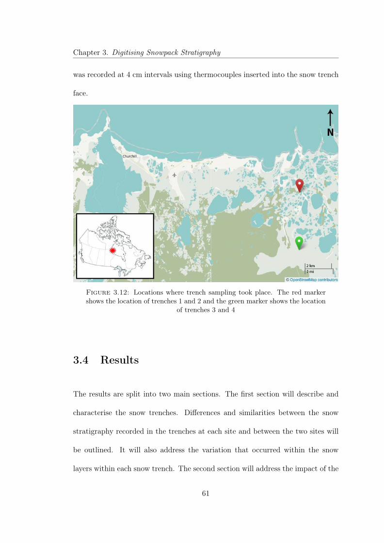
Chapter 3. Digitising Snowpack Stratigraphy
was recorded at 4 cm intervals using thermocouples inserted into the snow trench
face.
Figure 3.12: Locations where trench sampling took place. The red markershows the location of trenches 1 and 2 and the green marker shows the location
of trenches 3 and 4
3.4 Results
The results are split into two main sections. The first section will describe and
characterise the snow trenches. Differences and similarities between the snow
stratigraphy recorded in the trenches at each site and between the two sites will
be outlined. It will also address the variation that occurred within the snow
layers within each snow trench. The second section will address the impact of the
61

Chapter 3. Digitising Snowpack Stratigraphy
variation in snow properties within layers and within the snowpack on simulated
brightness temperatures from snow emission models.
3.4.1 Variation in snowpack properties and characteristics
During the winter of 2010-2011 the majority of snow accumulated from pre-
cipitation between December and January and while there were precipitation
events later in the season, the continuously high wind speeds encouraged wind
redistribution and thus snow depths remained shallow into the latter half of the
season (King et al., 2014).
Overall the snowpack was characterised as having 10 - 20 cm of depth hoar at
the base of the pack overlaid with wind and melt-refreeze crusts between layers
of wind slab. Depth hoar growth occurs when a strong temperature gradient is
present (Baunach et al., 2001). This is demonstrated by the increased thickness
of depth hoar in trenches 1 and 2 where depth hoar formed in the hummocks and
undulations on the tundra surface.
Figure 3.13 summarises the difference in snow depth and SWE for all for trenches.
Trenches 1 and 2 had a wider range of depths than Trenches 3 and 4, this was
caused by the more hummocky undulating subnivean topography but compara-
tively smooth snow surface at the open tundra site. At the fen site where trenches
3 and 4 were located the subnivean surface was much less hummocky. The snow
depth was greater at the open tundra site, although the SWE for that site was not
62

Chapter 3. Digitising Snowpack Stratigraphy
significantly greater. This is explained by the hard compacted, high density wind
slab which formed the upper part of the snowpack on the tundra site. The fen
site had a much softer looser upper snowpack consisting mainly of larger facetted
grains or freshly deposited snow which was decomposing on the surface. Figure
3.14 shows the variation which occurred within the snow layers in each snowpack,
the layers are organised so the bottom layer is on the right hand side of each plot,
and the upper on the left.
1 2 3 40
10
20
30
40
50
60
Trench
cm
SWEDepth
Figure 3.13: Difference in range of total snowpack SWE and Depth measure-ments across entire trench. The whiskers of each plot are the lowest or highestdatapoint within 1.5× the interquartile range. The boxes cover the 1st to thirdquartile the median marked by a line and the mean by a hollow circle, this
convention is used for all subsequent box plots.
63

Chapter 3. Digitising Snowpack Stratigraphy
Figure 3.14: Variation in snow properties within and between layers in eachtrench.
The stratigraphic information digitised from the snow trenches 1 to 4 is shown in
Figures 3.16 to 3.19 respectively, snow grain type symbols are taken from Fierz
et al. (2009) and a guide can be found in Figure 3.15. These Figures provide
a visualisation of the variation which exists within the layers of the snowpack.
Figure 3.20 shows how trenches 1 and 2 are related to each other spatially. By
considering Figures 3.16 and 3.17 in relation to Figure 3.20 (the colour scales
are identical) you can see that properties such as grain diameter and density
exhibit a similar level of variability in both trenches, and therefore in both spatial
64

Chapter 3. Digitising Snowpack Stratigraphy
directions. Trenches 1 and 2 varied more between orthogonal directions, the
impact of the wind is evident in the high number of discontinuous layers in trench
2 (5) compared to trench 1 (3). Additionally the depth of Trench 2 was much
greater, having an average depth of 38 cm compared to Trench 1 which had
an average depth of 28 cm. Between trench 3 and 4 there is less quantifiable
difference with both trenches consisting primarily of continuous layers and both
trenches having similar average depths, 18 cm compared to 22 cm.
d ueP RC
DFOh
- Rounded
- Partly Decomposed precipitation
- Solid Faceted
- Ice Layer
- Basal Ice Layer
- Rounded Facetted
- Facetted Rounded
- Hollow Cups
- Chains of Deph Hoar
- Melt Refreeze Crust
ed
Figure 3.15: Snow microstructure and grain type symbols used in this thesis(classification/symbols from Fierz et al. (2009))
The results of the random roughness metrics are shown in Figure 3.21. At the
base of the snowpack the greater roughness was observed at Trenches 1 and 2.
This reflected the more undulating subnivean topography at this site. However,
the roughness dropped off substantially towards the top of the snowpack, and
overall trenches 3 and 4 had a higher and more consistent level of roughness
throughout the snowpack.
65

Chapter 3. Digitising Snowpack Stratigraphy
Figure 3.16: Stratigraphy and snowpack properties of Trench 1, ice crusts aremarked in red on the top image
66
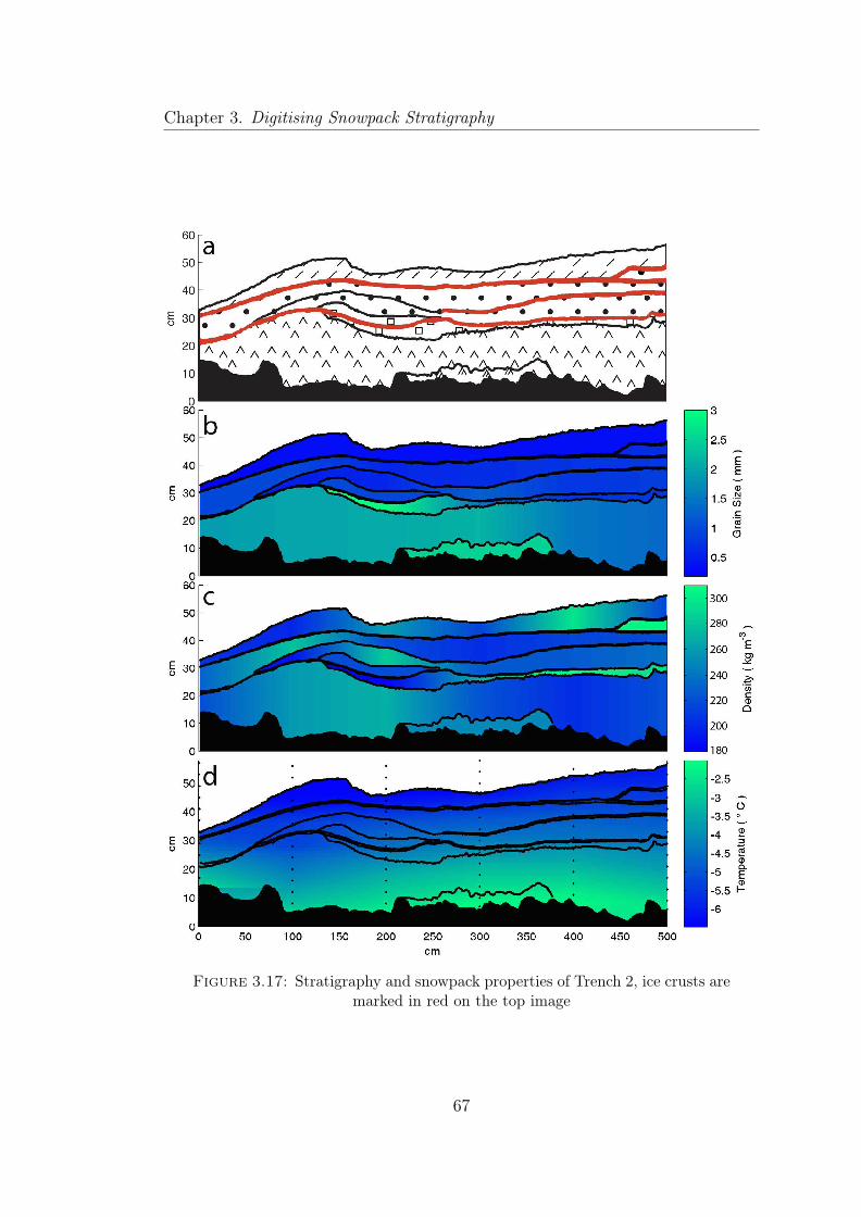
Chapter 3. Digitising Snowpack Stratigraphy
Figure 3.17: Stratigraphy and snowpack properties of Trench 2, ice crusts aremarked in red on the top image
67

Chapter 3. Digitising Snowpack Stratigraphy
Figure 3.18: Stratigraphy and snowpack properties of Trench 3, ice crusts aremarked in red on the top image
68

Chapter 3. Digitising Snowpack Stratigraphy
Figure 3.19: Stratigraphy and snowpack properties of Trench 4, ice crusts aremarked in red on the top image
69
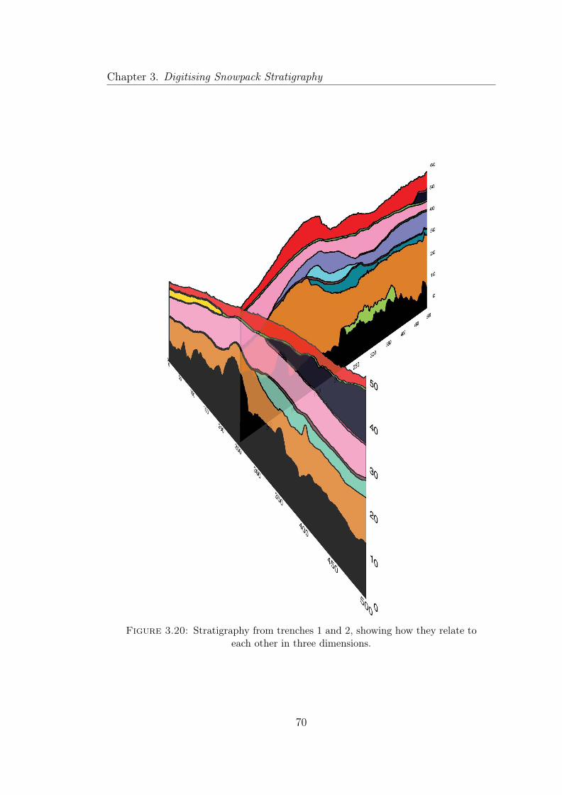
Chapter 3. Digitising Snowpack Stratigraphy
Figure 3.20: Stratigraphy from trenches 1 and 2, showing how they relate toeach other in three dimensions.
70

Chapter 3. Digitising Snowpack Stratigraphy
0
1
2
1 2 3 4 5 6 7 8 9 10 11
0
1
2
1 2 3 4 5 6 7 8 9 10 11 12 13
0
0.5
1
1 2 3 4 5 6 7 8
0
0.5
1
1 2 3 4 5 6 7 8 9 10
Layer boundary number
Tre
nch 1
Tre
nch 2
Tre
nch 3
Tre
nch 4
Figure 3.21: Boxplots for random roughness.
71

Chapter 3. Digitising Snowpack Stratigraphy
3.4.2 Variation in n-HUT model Tb
The n-HUT model was initialised with the trench stratigraphy data in three ways,
of increasing complexity
1. Bulk Properties: the average of all of the data collected over the course of
the trench was averaged into one layer, the n-HUT model was then used to
simulate the brightness temperature for this snow layer, the output can be
found in Table 3.1.
2. Layered average: The average of each layer is taken to produce one averaged
multi-layered snow profile. Properties of discontinuous layers were included
with adjacent layers so the overall mean depth was equal to the profile
depth. The results from these simulations can be found in Table 3.2.
3. Trench simulation: Properties were averaged for each layer and then the
n-HUT run for each horizontal profile. The mean and standard deviations
of the brightness temperature distributions can be found in Table 3.3 and
the distributions of the simulations found in Figures 3.22 to 3.25.
Table 3.1: Simulated brightness temperatures from using bulk snowpackproperties
Trench 19V 19H 37V 37H1 247 236 208 1992 244 233 194 1863 249 237 215 2054 249 238 219 210
72

Chapter 3. Digitising Snowpack Stratigraphy
Table 3.2: Simulated brightness temperatures from using averaged snowpackbased on trench data
Trench 19V 19H 37V 37H1 232 158 202 1412 233 176 188 1453 238 182 209 1614 233 163 209 148
Table 3.3: Mean and standard deviations of simulated brightness tempera-tures from trenches
MeanTrench1 19V 19H 37V 37H1 186 131 176 1252 206 149 179 1323 243 186 213 1654 239 167 214 151
Standard DeviationTrench 19V 19H 37V 37H1 1.41 5.22 3.74 6.232 2.89 8.89 7.82 9.093 0.62 0.46 3.37 2.504 0.78 1.16 4.00 3.15
Table 3.4 shows the differences between brightness temperature of each pair of
trenches in different orthogonal directions when the different methods of simu-
lating brightness temperature were used. When the bulk, one layer simulation
was used there was little difference between trench pairs, with the exception of
37 GHz for trenches 1&2. Overall the disparity between the pairs of trenches
increased the more complex the method of simulation used.
73

Chapter 3. Digitising Snowpack Stratigraphy
Tb (K)180 190 200 210
Freq
uenc
y
0
10
20
30
40
50
Tb (K)130 140 150 160
Freq
uenc
y
0
10
20
30
40
50
Tb (K)160 180 200 220
Freq
uenc
y
0
10
20
30
40
50
Tb (K)100 120 140 160
Freq
uenc
y
0
10
20
30
40
50
Figure 3.22: Histograms showing the distribution of Brightness Temperaturessimulations for Trench 1 when variable layer heights are used with the meanproperties for top-left)19V, top-right)19H, bottom-left)37V, bottom-right)37H
Table 3.4: The absolute difference in simulated brightness temperaturesbetween the pair of orthogonal trenches at each site. Three different methods
of using the trench data are compared
Freq/polariastion 1 layer Bulk n-layer mean from trenchTrench 1&2 19V 2.4 1.4 19.9
19H 2.7 18.3 18.337V 13.6 14.6 2.737H 13.4 4.7 7.6
Trench 3&4 19V 0.3 5.2 4.319H 0.9 19.7 19.337V 3.9 0.1 0.737H 4.3 13.8 13.3
Mean 5.2 9.7 10.8
74

Chapter 3. Digitising Snowpack Stratigraphy
Tb (K)180 190 200 210
Freq
uenc
y
0
10
20
30
40
50
Tb (K)130 140 150 160
Freq
uenc
y
0
10
20
30
40
50
Tb (K)160 180 200 220
Freq
uenc
y
0
10
20
30
40
50
Tb (K)100 120 140 160
Freq
uenc
y
0
10
20
30
40
50
Figure 3.23: Histograms showing the distribution of Brightness Temperaturessimulations for Trench 2 when variable layer heights are used withe meanproperties for top-left)19V, top-right)19H, bottom-left)37V, bottom-right)37H
75

Chapter 3. Digitising Snowpack Stratigraphy
Tb (K)230 235 240 245
Freq
uenc
y
0
10
20
30
Tb (K)165 170 175 180 185 190
Freq
uenc
y
0
10
20
30
Tb (K)200 210 220 230
Freq
uenc
y
0
10
20
30
Tb (K)150 160 170
Freq
uenc
y
0
10
20
30
Figure 3.24: Histograms showing the distribution of Brightness Temperaturessimulations for Trench 3 when variable layer heights are used withe meanproperties for top-left)19V, top-right)19H, bottom-left)37V, bottom-right)37H
76

Chapter 3. Digitising Snowpack Stratigraphy
Tb (K)230 235 240 245
Freq
uenc
y
0
10
20
30
Tb (K)165 170 175 180 185 190
Freq
uenc
y
0
10
20
30
Tb (K)200 210 220 230
Freq
uenc
y
0
10
20
30
Tb (K)150 160 170
Freq
uenc
y
0
10
20
30
Figure 3.25: Histograms showing the distribution of Brightness Temperaturessimulations for Trench 4 when variable layer heights are used withe meanproperties for top-left)19V, top-right)19H, bottom-left)37V, bottom-right)37H
77

Chapter 3. Digitising Snowpack Stratigraphy
3.5 Discussion
Quantifying snow stratigraphy from near-infrared photography has the potential
to introduce error into the digitised snow profile information, as a result of an
imperfect method of translating pixel co-ordinates from a photograph into a geo-
referenced location. While past methods of conducting this translation have
proved accurate on flat terrain such as frozen lakes, when applied to areas of more
varied subnivean terrain large errors are introduced to the digitised snow layer
boundary data. To address this problem a semi-automated method of quantifying
scale across a stitched snow trench image was developed, allowing for pixel co-
ordinates to be translated more accurately. An adverse effect of this method
was that discontinuities form in the image, where boundaries in the stitched
snow trench image occur. The impact of these artefacts was negated by applying
optimal smoothing to the layers at the image joins in an iterative manner. The
result is a more accurate method of quantifying snow trench stratigraphy from
near infra-red photography that is accurate on a variety of subnivean surfaces and
also offers a substantial improvement in efficiency over existing post-processing
methods.
The new method was used to measure layer boundary roughness from within the
snowpack, a property which has been shown to be important in radar applica-
tions (Rott and Mätzler, 1987; Ulaby et al., 1981) but whose impact on passive
microwave remote sensing is unknown. It has been demonstrated that there is
78

Chapter 3. Digitising Snowpack Stratigraphy
substantial variation within the snowpack, and that the degree of variation is
likely to depend on the roughness of the subnivean topography. Additionally, the
speed of the wind at a site may work to reduce the roughness in the upper layers,
and it is believed this was the case at our site, although, it is well documented
that very high wind speeds will lead to surface features such as drifts or sastrugi,
and so this hypothesis will require further investigation.
The improved accuracy of this method also allowed properties to be assigned to
snow layers based on in situ measurements, which removes the subjectivity from
previous work. Using this automated technique, the variation of the internal
properties of snow layers was investigated. This was found to vary significantly,
although the degree of variability was not substantially different when layers from
two different trenches at the same site were compared. This implies that one
trench is able to capture a significant amount of variability from within a snow
layer, although the variation in the stratigraphy itself is significant.
The impact that this variation had on the actual modelled brightness temperature
is interesting. The mean brightness temperature from two trenches at the same
site is usually very similar, often within sensor noise, when bulk values were
used. However, as the stratigraphy was represented with an increased level of
accuracy, more variation in brightness temperature simulations was found. Where
discontinuous ice layers were present the distribution of simulated brightness
temperatures for a trench split so that contained multiple peaks for vertically
79

Chapter 3. Digitising Snowpack Stratigraphy
polarised radiation. This demonstrates the significant impact that the presence
of even a very thin ice layer can have on a snow pack’s microwave signature.
80

Chapter 4
Improved measurement of ice layer
densities and application in snow
microwave emission models
4.1 Aims
The aim of this chapter, as set out in Chapter 1 is to improve the parameterisation
of ice layers in snow emission models by measuring and analysing the influence
of their structural properties (such as density and bubble size) on the accuracy
of simulated brightness temperatures. This will be achieved by addressing the
following three objectives. . .
1. To develop a new field method for measuring the density of ice layers
81

Chapter 4. Ice layer density
2. To compare simulated and observed brightness temperatures using mea-
sured ice layer densities to test the sensitivity of the MEMLS and DMRT-
ML snow emission models to changes in ice layer parameterisation
3. To examine the impact that any sensitivity could have on ice layer detection
algorithms
4.2 Measurements of ice layer density
4.2.1 Development of ice density measurement method
A new laboratory and field-based method was developed to measure the density
of ice layers found in seasonal snow, based on volumetric displacement. The basic
principle is that when an ice layer sample is submerged in a vessel of liquid, calcu-
lating the volume displacement and sample mass will yield an estimate of density.
The laboratory and field protocol for measuring the density of ice layers with this
method is outlined in Figure 4.1. The mass of a sealed 50 ml centrifuge tube with
2.5 ml graduations containing white spirit (sometimes termed ’mineral spirits’),
was measured with a precision of ±0.001 g under laboratory conditions before
entering the field. White spirit is immiscible with water and has a low freezing
point (-70◦C), which means it can be used at temperatures < 0◦C eliminating
potential sample melt. White spirit also has a low density (650 kg m−3), making
it likely that the ice sample would sink and be completely submerged. In the
82

Chapter 4. Ice layer density
field the centrifuge tube was held by a fixed, levelled, mounting system within
the macro setting range of a compact camera. Each camera image was centred
on a visible datum on the mounting system to ensure the camera was correctly
focused, and that repeat images were consistently made from the same horizontal
position. Images were taken before and after each ice sample was submerged as
shown in Figure 4.2.
Figure 4.1: Flow chart describing the methodology to measure densities ofice samples from a snowpack
In each image three positions were identified during post processing: the liquid
level, the graduation above the liquid level and the graduation below the liquid
level. Pixel co-ordinates of these positions were taken and as the volume of the
graduations on the centrifuge tube were known, and their location in pixels known,
83

Chapter 4. Ice layer density
Figure 4.2: Example of pair of photos used in calculation of ice sample volume.A, taken before the sample was added and B, taken after. V is equal to thevolume of the ice sample. Black lines are guides added to help assess the quality
of the photos.
the height of the liquid level in pixels could be translated to a volume in ml at a
higher resolution than just the centrifuge tube graduations would allow. The top
of the liquid level was located rather than the meniscus for ease of identification;
as relative volume change was used no error was introduced. After images were
taken, the centrifuge tube containing the sample was sealed and the change in
mass was measured on return to the laboratory. Only samples where the liquid
84

Chapter 4. Ice layer density
in the tube was level in both images and the sample was short enough to be fully
submerged were used in analysis.
4.2.2 Methodological error
Ice layers found in snowpacks are very difficult to accurately and consistently
re-create under laboratory conditions. Therefore to assess the accuracy of the
ice density measurement technique, ball bearings of known volume were mea-
sured. Stainless steel ball bearings were used (manufactured to a diameter of
1 cm ±2.5× 10⁻⁵ cm), resulting in a volume range of 0.5236 cm3 ± 0.0004 cm3.
The volume of the ball bearings was calculated from photos of the before and after
images of 10 ball bearings submerged in the centrifuge tube. The expected total
volume of all ball bearings of approximately 5.236 cm3 is comparable to the mean
volume of ice samples collected in the field during pilot studies. Of 134 samples,
each consisting of 10 ball bearings, the mean volume was 5.045 cm3. The volume
measurements were normally distributed and an error value based on ±1 standard
deviations was calculated, resulting in a systematic volume measurement error or
bias of −0.19 cm3.
The largest source of error is in reading the height of the liquid in the centrifuge
tube from the camera photos. Identifying the precise height of the surface of
the liquid between the graduation markings on the cylinder is limited by the
quality of the camera focus and resolution of the camera. If the camera focus
85

Chapter 4. Ice layer density
is not perfect it is difficult to perfectly locate the height of the liquid, and error
and uncertainty occurs. Based on carrying out 10 repeat measurements on 10
centrifuge tube photos we estimate the error to be ±0.125 cm3 in each volume
measurement photo, equating to a root mean squared error in the measurement
of the ice sample volume of ±0.18 cm3, as each volume measurement involves
reading the volume from two photos.
To calculate the optimum sample volume the number of ball bearings used in
each volume measurement was increased from 1 to 24, a volume range of 0.52
cm3 to 12.57 cm3. Correlation between standard deviation and sample volume
was not statistically significant (confidence >99%), demonstrating that the error
in volume measurement was independent of sample volume. Field trials suggested
that 10 cm3 was the maximum sample volume routinely possible to use due to
the diameter of the centrifuge tube. Although no minimum sample volume was
set, effort was always taken to obtain the largest possible.
To estimate the potential impact of the uncertainty in volume measurement on
samples taken in the field, the random (±0.18 cm3) volume measurement error
from the ball bearing experiment was applied to a theoretical ice sample of
volume 4.89 cm3 and mass 4.53 g (equating to a density of 916 kg m−3). This
volume error from the ball bearing experiment translated into an observed volume
range of 4.53 - 4.89 cm3 (i.e. 4.71 cm3 ± 0.18 cm3). Assuming no error in the
balance (precision of ±0.001 g), the upper density value (minimum volume) was
951 kg m−3 and the lower density value (maximum volume) was 881 kg m−3,
86

Chapter 4. Ice layer density
representing an uncertainty in density of ±35 kg m−3 or 4%. The impact of the
error was estimated to be low enough to justifying the practical application of
this technique.
4.2.3 Field Measurements
4.2.3.1 Ice layer measurements
During the winter of 2013, ice layer density measurements were collected at three
sites in Canada: North Bay, Ontario (46.33◦N, 79.31◦W) between 8-9 February,
CARE, Egbert, Ontario (44.23◦N, 79.78◦W) on 25 February, and Trail Valley
Creek, Inuvik, North West Territories (68.72◦N, 133.16◦W) on 9 April.
In North Bay, information on the snow stratigraphy, density and the mean maxi-
mal extent of individual snow grains was collected in a woodland clearing. Ground
based radiometers were used to collect brightness temperatures at this site. An
artificial ice layer was created on the surface of the snowpack and compared with
naturally formed ice layers. Artificial ice layers have been created in previous
work (Montpetit et al., 2012) so it is important to know if their characteristics
differ from naturally occurring ice layers. To create the layer a very thin top layer
of undulating recent snow (less than 6 hours old) was swept from the snowpack
to expose a melt crust below, this was done to maintain an ice layer of even
thickness across the site. After the removal of recent snow, water was sprayed onto
the snowpack to create a surface ice layer (air temperatures were approximately
87

Chapter 4. Ice layer density
-20◦C). A natural ice layer covering the entire clearing was also present lower
within the snowpack (formed by 2 mm of rain on 30 January). Density, bubble
diameter, and thickness measurements of both natural and artificial ice layers
were made; whenever bubbles were visible their diameters were measured using a
field microscope and snow grain card, a resolution of 0.1 mm was possible with the
field microscope. Very small bubbles, with a diameter of < 0.1 mm were recorded
as being visible although a diameter could not be applied to them. Layer thickness
was measured to a resolution of 1 mm for each sample. 15 density measurements
were made of the natural and 15 of the artificial ice layer.
At CARE, measurements were conducted in an open, grass-covered field. A
spatially continuous ice layer formed over an area of at least 200× 100 m in the
10 cm deep snowpack as a result of above-freezing daytime temperatures for a
period of 4 days prior to measurement; ice layer thickness and densities were
measured in the same manner as in North Bay, 29 measurements of ice density
and thickness were made.
In Inuvik, water was sprayed onto a 30 cm tundra snowpack when air tempera-
tures were approximately -25◦C to form an artificial ice layer on the surface of
the snowpack as no natural ice layer was present. Water was sprayed over an area
of 1 m2, concentrating the spraying towards one edge, creating an ice thickness
gradient that allowed 28 measurements of ice layer density across a range of ice
layer thicknesses.
88

Chapter 4. Ice layer density
4.2.3.2 Brightness Temperature observations
Brightness temperatures were measured at 19 and 37 GHz using portable surface-
based microwave radiometers (dual polarisation, ≈ 1.5 m above the snow, 52.5◦
incidence angle, sampled at a 1 second integration time and averaged over 3
minutes) at the North Bay field site. Radiometers were calibrated using a two-
point procedure, before and after field measurements, using a microwave absorber
at ambient temperatures (warm target) and another cooled by liquid nitrogen
(cold target) (Solheim, 1993). A non-linear iterative procedure was used to
account for sensor drift between calibrations before and after field measurements;
coefficients for converting target, load and noise diode voltages into brightness
temperatures were calculated. As a result, brightness temperature measurements
were produced to an accuracy of <2.0 K (Derksen et al., 2012a). After brightness
temperatures were recorded, a snow pit was excavated in the radiometer footprint
to measure a vertical profile of snow stratigraphy, temperature, grain diameter
(mean maximal diameter) and density.
4.3 Results: Ice layer measurements
4.3.1 Ice layer bubble size and thickness
Table 4.1 summarises the measurement of ice layer thickness and bubble size.
In some cases bubbles were visible in the ice layer, but were not large enough
89

Chapter 4. Ice layer density
to be measured using the field microscope. These were noted as < 0.1 mm in
Table 4.1. For the purpose of calculating the mean and standard deviation of the
bubble distribution a value of 0.05 mm was applied to these bubbles. There was
no correlation between ice layer thickness and bubble diameter.
Table 4.1: Measurements of ice layer bubble size and thickness (all sizes inmm)
Bubble Diameter Layer ThicknessType n n < 0.1 Mean SD n Mean SD
CARE Natural 0 - - - 29 8 0.6North Bay Natural 14 4 0.16 0.12 15 3 0.6
Artificial 12 6 0.08 0.03 15 5 0.9Inuvik Artificial 0 - - - 28 2 0.5
Overall - 26 10 0.12 0.1 86 5 2.7
4.3.2 Ice layer density
Mass and volume measurements were made of 86 samples of ice layers and are
summarised in Table 4.2 and Figure 4.3. The mean sample volume was 6.4 cm3
meaning the random error on the density measurements was ±18kgm−3. Ice layer
densities varied between 841 and 980 kg m−3, with an overall mean of 909 kg m−3
and standard deviation of 23 kg m−3. Natural ice layers were on average less dense
than artificial ones although the difference was within the methodological error.
Table 4.2: Ice layer density measurements, (all values have been corrected toaccount for the measured −0.19cm3 bias in volume)
Site n Mean (kg m−3) SD (kg m−3)CARE 29 906 17North Bay - Natural 15 890 21North Bay - Artificial 15 921 18Inuvik 28 915 26
90

Chapter 4. Ice layer density
Figure 4.3: Summary of ice layer density measurements. Stacked histogramshowing frequency of each density measurement, colours show distribution of
artificial and natural ice layers across multiple sites
4.3.3 Error in measured density
Three sources of error were identified, the systematic error that exists in the
method used to measure the volume of the ice samples (and would apply to any
object measured using this method) which was described in the methodological
error section, the random error in the method and the error from sample porosity,
(which applies only to the measurement of ice layer density using the submersion
method). In this section we will quantitatively assess the impact these sources of
error on the measurements of ice layer density.
91

Chapter 4. Ice layer density
The measured ice layers had a closed porosity, where the layers contained bubbles
but they were not connected in a porous structure. However, due to the presence
of bubbles in the ice layers some increase in porosity would occur when the ice
layer was broken and placed in the centrifuge tube, this is called the effective
porosity.
To quantitatively evaluate the effect of effective porosity on the ice layer density
measurements, the ice layer, and the bubbles within it were numerically modelled.
The ice layer was represented using spheres, representing air bubbles scattered
randomly within an ice sample of size x, y, z and density d.
We randomly placed spheres within the x, y, z co-ordinate system without any
overlap. The size of the spheres was determined by taking a random sample
from a normal distribution of bubble sizes based on a given mean and standard
deviation. A sphere size was chosen from the random sample and located at
random within the x, y, z axes, if that sphere in that location overlapped another
sphere then the location was changed. If after 1000 attempts a location for the
sphere could not be found its radius was changed to another random sample from
the normal distribution and the process repeated. After each sphere was placed,
the total volume of all the spheres and the density of the ice sample was calculated.
Spheres were added to the sample until the desired density was reached.
Slices were taken through the ice sample and the volume of the spheres that would
be open to the surface (and therefore allow liquid to penetrate the ice surface)
92
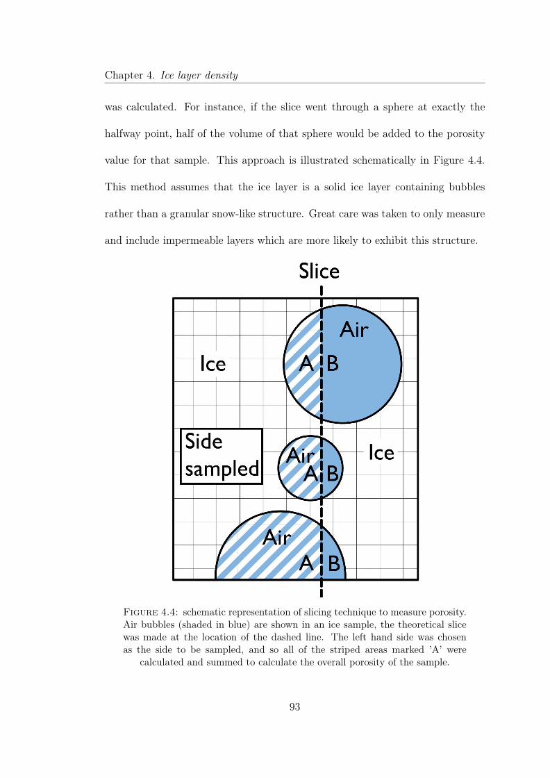
Chapter 4. Ice layer density
was calculated. For instance, if the slice went through a sphere at exactly the
halfway point, half of the volume of that sphere would be added to the porosity
value for that sample. This approach is illustrated schematically in Figure 4.4.
This method assumes that the ice layer is a solid ice layer containing bubbles
rather than a granular snow-like structure. Great care was taken to only measure
and include impermeable layers which are more likely to exhibit this structure.
Figure 4.4: schematic representation of slicing technique to measure porosity.Air bubbles (shaded in blue) are shown in an ice sample, the theoretical slicewas made at the location of the dashed line. The left hand side was chosenas the side to be sampled, and so all of the striped areas marked ’A’ were
calculated and summed to calculate the overall porosity of the sample.
93
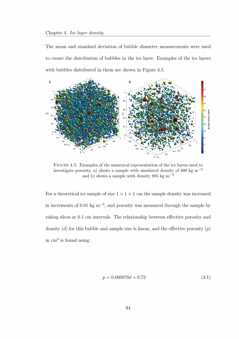
Chapter 4. Ice layer density
The mean and standard deviation of bubble diameter measurements were used
to create the distribution of bubbles in the ice layer. Examples of the ice layers
with bubbles distributed in them are shown in Figure 4.5.
Figure 4.5: Examples of the numerical representation of the ice layers used toinvestigate porosity, a) shows a sample with simulated density of 800 kg m−3
and b) shows a sample with density 885 kg m−3
For a theoretical ice sample of size 1× 1× 1 cm the sample density was increased
in increments of 0.01 kg m−3, and porosity was measured through the sample by
taking slices at 0.1 cm intervals. The relationship between effective porosity and
density (d) for this bubble and sample size is linear, and the effective porosity (p)
in cm3 is found using:
p = 0.000078d+ 0.72 (4.1)
94

Chapter 4. Ice layer density
this assumes the same porosity on all edges of the ice sample (where the sample
was broken). The bubble diameter mean and standard deviation were taken as
the overall values from all samples. To calculate the impact of this porosity on
our samples we assumed a sample width of 2 cm (the width of the centrifuge
tube), we measured the sample thickness and we measured the volume (with
known methodological error) so we were able to estimate the maximum and
minimum dimensions of each sample. By using the relationship in Equation 4.1
we estimated the porosity of each sample based on the measured density. Sample
porosities ranged from 6.5× 10⁻⁵ to 0.0001 cm3. The mean increase from using
either the maximum or minimum value for density in the porosity calculations
was 1.42× 10⁻⁶ cm3.
The maximum random error (±0.18 cm3), the volume measurement bias (−0.19 cm3)
and the porosity correction were applied to each of the volume measurements and
the maximum range of density calculated for each sample. Due to the very high
densities of the samples porosity was negligible (less than 0.0001 cm3). Overall
the measurements of ice layer density (909± 18 kg m−3) were not significantly
different to measurements of pure ice.
95

Chapter 4. Ice layer density
4.4 Simulation of brightness temperatures using
measured ice density
Objective measurements of ice layer density with fully characterised uncertainty
(see previous section) were applied to the representations of ice layers in snow
emission models. In this section we: 1) outline how ice layers are represented
in snow emission models and how the models were initialised, 2) describe how
we initialised the snow emission models and, 3) present the impact of measured
ice layer densities on simulation bias of brightness temperatures, and the impact
on the polarisation ratio method of detecting ice layers (Grenfell and Putkonen,
2008).
4.4.1 Model Initialisation
4.4.1.1 DMRT-ML
The vertical profile of snow properties measured at North Bay (Figure 4.6) was
used to initialise both snow emission model simulations. The two layers directly
beneath the artificial surface crust were merged together for model initialisation
as an exact lower boundary was not evident in the stratigraphy; an average grain
diameter of both layers was used (0.95 mm).
96

Chapter 4. Ice layer density
The measured soil temperature was -2◦C and an assumed soil permittivity value
of 6-j was used (Zhang et al., 2003). The n-HUT soil model was used in the
DMRT-ML model runs (as in Roy et al. (2013)). The bubble diameter in ice
layers was set to 0.12 mm, as 0.12 mm was the mean bubble size recorded across
all ice layer samples. In later sections, the properties of the ice layers were scaled
to investigate the sensitivity of model output to specific parameters based on our
observations. Model initialisation values are summarised in Table 4.3.
Table 4.3: Summary of range of input and initialisation parameters across allmodel runs
Measured ModelledType T (cm) Da Gd
b Bdc Temp(◦C) D Gd Bd lcd P
Ice 0.5 909 - 0.2 -13 500 - 916 - 0.2 - 0.5 0.67 -Snow 17.75 330 0.95 - -7 330 0.95 - 0.17 -Ice 0.25 909 - 0.2 -1 500 - 916 - 0.2 - 0.5 0.67 -Snow 2.5 340 1.35 - -1 340 1.35 - 0.20 -Ice 1 909 - 0.2 -0.73 500 - 916 - 0.2 - 0.5 0.67 -Soil - - - - -2 - - - - 6-j
aDensity (kg m−3)bGrain Diameter (mm)cBubble Diameter (mm)dCorrelation Length (mm)
97

Chapter 4. Ice layer density
Figure 4.6: Observed and modelled snowpack at North Bay, explanation ofsnow symbols in figure 3.15
4.4.1.2 MEMLS
MEMLS was initialised using the same snowpack stratigraphy as DMRT-ML
(as shown in Figure 4.6). Density and temperature parameters were directly
transferable between models. MEMLS does not use the grain size parameter to
define snow microstructure but rather correlation length. Initialisation values are
98

Chapter 4. Ice layer density
shown in Table 4.3. For snow layers, the grain size of the layer was converted into
a correlation length using the relationship in Equation 4.2 presented in Durand
et al. (2008)
pex =
⎧⎪⎪⎪⎨
⎪⎪⎪⎩
0.18 + 0.09 ln Dmax, v > 0.2 and Dmax > 0.125 mm
p0, otherwise
(4.2)
where pex is the exponential correlation length, Dmax is the largest measured
extension of the snow grain, and v is the volume fraction (snow density divided
by density of ice). In the case of ice layers a correlation length of 0.71 mm was
used as this value is suggested as a suitable value for ice crusts in Matzler and
Wiesmann (1999).
4.5 Results: Brightness temperature simulations
This section is split into three parts: firstly a sensitivity analysis was conducted
on the parameters used to describe ice layers in both DMRT-ML and MEMLS,
secondly the models were tuned to find the optimum ice layer density to minimise
bias and, thirdly the impact of ice layer density on the polarisation and gradient
ratios used in ice layer detection was investigated.
99

Chapter 4. Ice layer density
4.5.1 Model Sensitivity to ice layer properties
The models were initialised using the snowpack observed at the North Bay field
site and described in section 4.4.1. Each snowpack input parameter was varied
individually between a range of values typically found in shallow snowpacks. The
percentage change in the model output was recorded for each iteration. The
results from the MEMLS and DMRT-ML models are discussed below.
4.5.1.1 MEMLS
MEMLS has no ice layer specific parameters, it describes an ice layer using the
same parameters as are used to describe any snow layer. These are: density,
thickness, temperature and correlation length, the sensitivity to these parameters
is shown in Figure 4.7.
Ice layer density was varied between 500 and 900 kg m−3. Between 500 and
600 kg m−3 jumps are visible in the sensitivity plot. These jumps are caused by
coherence effects as the ice layer switches from a coherent to incoherent layer, this
occurs at a slightly different density for both 19GHz and 37GHz which explains
the offset between the two. H-Pol is more sensitive to ice layer density than V-pol.
Coherence is dependent on layer thickness and density, and this is demonstrated
again in the rapid changes in sensitivity which are visible in the ice layer thickness
sensitivity plot between 0.01 and 5 mm. For 37 GHz both H-pol and V-pol
demonstrate virtually the same sensitivity profile to ice layer thickness, with
100

Chapter 4. Ice layer density
only a small difference when the layers are incoherent at very low thicknesses.
Correlation length and temperature both exhibit much lower sensitivity compared
to ice density or ice layer thickness.
Ice Density (kg m-3
)
500 600 700 800 900
% C
han
ge T
b
-10
0
10
20
30
40
19 GHz V-pol
19 GHz H-pol
37 GHz V-pol
37 GHz H-pol
Ice Temp (mm)
-40 -30 -20 -10 0%
Ch
an
ge T
b-5
-4
-3
-2
-1
0
Ice Thickness (mm)
0 1 2 3 54
% C
han
ge T
b
-30
-20
-10
0
10
20
30
Correlation Length
0 0.2 0.4 0.6 0.8
% C
han
ge T
b
0
0.5
1
1.5
2
2.5
Figure 4.7: Sensitivity of MEMLS to ice layer properties
4.5.1.2 DMRT-ML
Unlike MEMLS, DMRT-ML uses an ice layer specific parameter, bubble radius, to
describe the microstructure of the ice layer, it does not use a grain size parameter
for ice layers. In addition to the bubble radius parameter ice layers are assigned
a temperature, density and thickness, the same parameters which are used for
101

Chapter 4. Ice layer density
snow layers. The model sensitivity to these parameters is shown in Figure 4.8.
Sensitivity to ice layer density was of a similar magnitude to MEMLS, although
different in character. DMRT-ML does not include simulation of coherence effects,
and this leads to a more linear model sensitivity to this parameter, with the jumps
that were exhibited in the MEMLS sensitivity curve absent for DMRT-ML. DM-
ML is more sensitive to changes in ice layer temperature than MEMLS, and has
similar overall sensitivity to layer thickness at very low thicknesses. However, for
thicker layers, changes in layer thickness had much less effect on DMRT-ML than
MEMLS. The bubble radius parameter had a very low sensitivity.
Ice Density (kg m-3
)
500 550 600 650 700 750 800 850 900
% C
ha
ng
e T
b
0
5
10
15
20
25
30
35
19 GHz V-pol
19 GHz H-pol
37 GHz V-pol
37 GHz H-pol
Ice Temperature (oC)
-40 -35 -30 -25 -20 -15 -10 -5 0
% C
ha
ng
e T
b
-14
-12
-10
-8
-6
-4
-2
0
Ice Thickness (mm)
0 1 2 3 4 5
% C
ha
ng
e T
b
-40
-30
-20
-10
0
10
20
30
Ice layer bubble radius (microns) × 104
0 1 2 3 4 5
% C
ha
ng
e T
b
× 10-13
-3
-2
-1
0
1
2
3
Figure 4.8: Sensitivity of DMRT-ML to ice layer properties
102

Chapter 4. Ice layer density
4.5.2 Model optimisation using ice layer density
The results of the sensitivity analysis in section 4.5.1 show that V-pol exhibited
limited sensitivity to ice layer density compared to H-pol. Based on this the
models were tuned to minimise bias for the V-pol simulations. The observed
brightness temperatures are shown in Table 4.4 and have an accuracy of ± 2K
(Asmus and Grant, 1999).
Table 4.4: Observed brightness temperatures
37 V 37 H 19 V 19 H208 203 250 232
To minimise bias for V-pol simulations the microstructure parameter for both
DMRT-ML (Grainsize) and MEMLS (correlation length) was tuned using a scal-
ing factor. The microstructure parameter was chosen as snow and ice microstruc-
ture is difficult to quantify using a field microscope (as was used here) and so
there is some inherent uncertainty in the grain size and converted correlations
lengths measured in the field. For DMRT-ML the mean bias was zero when the
scaling factor was 2.252 and for MEMLS the mean bias was zero when the scaling
factor was 0.95.
After applying the optimum scaling factor to the model initialisation data in
order to minimise bias for the V-pol simulations the ice layer density at which
H-pol simulation bias was minimised was calculated. Ice layer density was varied
from 500 kg m−3 to 916 kg m−3 and model bias was minimised at 497 kg m−3
for DMRT-ML and 504 kg m−3 for MEMLS, results from the optimisations are
103

Chapter 4. Ice layer density
shown in figures 4.10 (DMRT-ML) and 4.9 (MEMLS). For DMRT-ML mean bias
across both frequencies and polarisations was −7.5K and for MEMLS mean bias
was −7.7K.
Ice Density (kg m-3)400 450 500 550 600 650 700 750 800 850 900
Mod
elle
d - O
bser
ved
TB (K
)
-70
-60
-50
-40
-30
-20
-10
0
10
2019 GHz V-pol19 GHz H-pol37 GHz V-pol37 GHz H-pol
Figure 4.9: Difference between modelled and observed brightness tempera-tures with changing density for MEMLS
104

Chapter 4. Ice layer density
Ice Density (kg m-3)400 450 500 550 600 650 700 750 800 850 900
Mod
elle
d - O
bser
ved
TB (K
)
-60
-40
-20
0
20
40
6019 GHz V-pol19 GHz H-pol37 GHz V-pol37 GHz H-pol
Figure 4.10: Difference between modelled and observed brightness tempera-tures with changing density for DMRT-ML
4.5.3 Effect of ice layer density on polarisation and gradient
ratios
Figures 4.11 and 4.12 show the impact of varying ice layer density (between
500 kg m−3 and 916 kg m−3) on the gradient ratio
GR(37, 19) =[TB(p, 37GHz)− TB(p, 19GHz)][TB(p, 37GHz) + TB(p, 19GHz)]
(4.3)
and polarisation ratio
105

Chapter 4. Ice layer density
PR(v) =[TB(V-Pol, v)− TB(H-Pol, v)][TB(V-Pol, v) + TB(H-Pol, v)]
(4.4)
used in the ice layer and rain-on-snow detection algorithm presented by Grenfell
and Putkonen (2008). The gradient ratio from the observed brightness temper-
atures was -0.0917 for V-pol and -0.07 for H-Pol and was not well simulated by
either model. MEMLS’ simulation of gradient ratio had far higher sensitivity to
ice layer density than DMRT-ML’s.
The observed polarisation ratio for 19 GHz was 0.0373, both MEMLS’s and
DMRT-ML’s simulations of polarisation ratio were similarly sensitive to changes
in ice density. The biases in the simulated polarisation and gradient ratios were
minimised when a low, physically unrealistic, ice layer density was used.
106

Chapter 4. Ice layer density
Ice Density (kg m-3)400 450 500 550 600 650 700 750 800 850 900
Gra
dien
t Rat
io
-0.16
-0.14
-0.12
-0.1
-0.08
-0.06
-0.04
-0.02
0
0.02
MEMLS v-polMEMLS h-polDMRT v-polDMRT h-pol
Figure 4.11: Effect of density on gradient ratio
Ice Density (kg m-3)400 450 500 550 600 650 700 750 800 850 900
Pola
risat
in R
atio
(19G
Hz)
0.02
0.04
0.06
0.08
0.1
0.12
0.14
0.16
0.18
0.2MEMLSDMRT-ML
Figure 4.12: Effect of density on polarisation ratio
107

Chapter 4. Ice layer density
4.6 Discussion and Conclusions
A new laboratory and field protocol was used to produce direct estimates of ice
layer density (including uncertainty). Measurements of natural and artificially
made ice layers produced an average density of 909± 18 kg m−3. The uncertainty
terms are related to systematic bias in the method used to measure the volume
of the ice samples, and the effective porosity of ice layers. Our measured density
values are higher than those in Marsh (1984) (mean 800 kg m−3), and Pfeffer and
Humphrey (1996) (400 kg m−3 to 800 kg m−3). It is unclear whether previous
studies assessed and quantified the density of ice layers that were permeable and
porous, including thin, non-continuous ice layers, which may explain the density
differences.
Characterisation of ice layer properties is of fundamental importance for the
application of snow emission models. When used in two different emission mod-
els (MEMLS and DMRT-ML) our ice layer measurements show that physically
unrealistic ice layer density values are necessary to optimise agreement between
simulations and observations. For the North Bay snowpack presented in this
study, bias was minimised when an ice layer density of between 497 kg m−3 and
504 kg m−3 was used. This is consistent with Durand et al. (2008) who used
ice layer densities of 500 kg m−3 to improve agreement between simulations and
microwave observations. The soil beneath the snowpack also has an impact on
108

Chapter 4. Ice layer density
the accuracy of brightness temperature simulations, although it has not been
included in this study.
Calculations of absorption occurring in a planar ice layer are well established,
modelling bubbly ice has produced good results in other scenarios (Dupont et al.,
2014) and changing the bubble diameter within the ice layer (in DMRT-ML)
has negligible impact on simulation bias. Consequently, this suggests simulation
bias does not result from radiative transfer within the ice layer, but rather at
layer boundaries where a high dielectric gradient leads to increased uncertainty
in simulated brightness temperatures. Montpetit et al. (2012) hypothesises that
MEMLS will better cope with these kinds of simulations as it models coherence
effects, however, in this case MEMLS has not performed better than DMRT-ML
(which does not include coherence effects).
As the predicted frequency of winter melt events increases, so will the need to
detect melt and rain on snow events (Montpetit et al., 2012). One possible method
of doing so would be to detect the existence of ice layers (Grenfell and Putkonen,
2008). We have also shown that ice layer density strongly impacts the polarisation
ratio used in ice layer detection algorithms (Figure 4.12). Future work in this
area should account for density if snow emission models are used. Currently
snow emission models are unable to correctly simulate ice layers when physically
realistic values of ice layer density are used. Future work is necessary, therefore,
to address the disconnect between observed ice layer properties and the necessary
ice layer inputs to optimise emission model performance.
109

Chapter 5
Snow Trenches in Inuvik
5.1 Introduction
In this chapter an array of snow trenches, varying in length from 5 to 50 m, is used
to capture variability within snowpack stratigraphy, layer boundary roughness
and simulated brightness temperatures over these scales. Subnivean topography
is far rougher and more undulating than the snow surface, we hypothesise that
the roughness of snow layers decreases with distance away from the ground, a
relationship would be useful for applying snow pack and snow emission models in
two dimensions.
110

Chapter 5. Trail Valley Creek
5.2 Aims and Objectives
The research question of this chapter is: "What is the impact of stratigraphic
variability on spatial distribution of brightness temperatures in a snow covered
tundra environment?" This question will be answered by addressing three aims
and achieving their associated objectives outlined below each aim.
• Aim 1 : To quantify layer thickness and boundary roughness variability
1. To test our hypothesis that snow layer boundary roughness is a func-
tion of the proportional height of the boundary in the snowpack and
ground roughness
2. To quantify the spatial variation in layer thickness in an Arctic tundra
watershed
• Aim 2 : To quantifying the impact of spatial variability of stratigraphy on
Snow Microwave Emission Models
1. To simulate brightness temperatures continuously along 5 and 50 metre
transects taken from Arctic tundra snowpacks
2. To compare simulated brightness temperatures at different spatial scales
and at different locations within one snowpack.
• Aim 3 : To determine the minimum subset size in each trench location
required to calculate the mean brightness temperature for that trench.
111

Chapter 5. Trail Valley Creek
5.3 Field Methods
The data requirements for this chapter were to have a large number of trenches,
long enough to capture local variability in snowpack stratigraphy, distributed over
a single land surface type with in situ measurements to enable snow emission
models to be run at each location. The general trench sampling method used
in Chapter 3 was also used to collect data for this chapter. Some modifications
were applied, which are described in Section 5.3.2.1. The Arctic tundra location
of Trail Valley Creek in Inuvik NWT, Canada was chosen to be the location of
the snow trenches.
5.3.1 Field Site
To achieve the research aims of this work a large number of snow trenches was
required on one land cover type and in one area. The location of Trail Valley Creek
in Inuvik NWT, Canada was chosen for this as it provided a small watershed with
large areas of flat tundra suitable to the excavation of many trenches quickly and
efficiently.
Figure 5.1 shows the location of Trail Valley creek at the margin of the Mackenzie
River Delta. Data was collected at the watershed over two periods during March
and April 2013.
112

Chapter 5. Trail Valley Creek
Figure 5.1: Landsat image and map showing the location of Trail ValleyCreek to the East of the Mackenzie Delta in NWT.
Trail Valley creek experiences a climate typical of the Canadian Arctic, winter
temperatures typically range from -35 to -15 C and high wind speeds of 10 to
15 ms−1 are regularly experienced throughout the winter (winter meteorological
summary shown in Figure 5.2). The tundra is a largely flat undulating surface
crossed by gullies and dotted with a vast array of lakes and ponds. During the
early season (before December) snow begins to infill the undulations in the tundra
and the gullies where the vegetation height is greater (willows as opposed to scrub
113
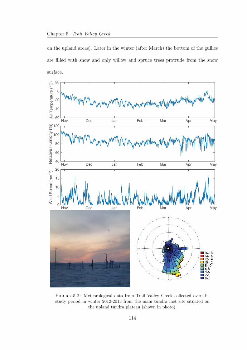
Chapter 5. Trail Valley Creek
on the upland areas). Later in the winter (after March) the bottom of the gullies
are filled with snow and only willow and spruce trees protrude from the snow
surface.
Figure 5.2: Meteorological data from Trail Valley Creek collected over thestudy period in winter 2012-2013 from the main tundra met site situated on
the upland tundra plateau (shown in photo).
114

Chapter 5. Trail Valley Creek
5.3.2 Field Measurements
5.3.2.1 Application of NIR trenches to distances >50 m
Snow trenches were excavated and used to obtain a large number of snowpack
profiles from each site, allowing snowpack variability to be characterised. In order
to ensure that as much variability was recorded at each site as possible trenches
of 50 m were used. A 50 m trench was dug using ten 5 m trenches situated next to
each other. This process was carried out over multiple days, and each 5 m section
processed individually using the methods described in Chapter 3. In order to
stitch each 5 m section together horizontal and vertical rulers were attached to a
board which was visible at the start and repositioned to appear at the end of each
5 m section (shown in Figure 5.3), as the board was not moved between the start
and end of each section it was able to act as a point of reference for the trench
sections to be aligned in the NIR trench photographs. The method used to stitch
the 5 m sections together is the same as the method used to smooth the artefacts
and discontinuities which occured between photographs in a 5 m trench.
115

Chapter 5. Trail Valley Creek
Figure 5.3: Photo showing collection of snowpack data from Trench 4 in TrailValley creek
5.3.2.2 Trench measurements
Snow trenches were excavated in March and April, Figure 5.4 shows the locations
that the trenches and pits were excavated. In Figure 5.4 land cover classifications
(Tundra, shrub and willow, and Forest) were created using a LiDAR derived
land surface classification as detailed in Marsh et al. (2010) and this was used
to classify the land surface on which the trenches were excavated, in addition to
local knowledge about the land surface obtained from members of the team who
had visited the field site during snow free times of year.
In the trenches measurements of snowpack properties were made every 5 m. This
116

Chapter 5. Trail Valley Creek
equates to one stratigraphic profile for a 5 m trench and 10 for a 50 m trench. The
horizontal location of the stratigraphic profile within every 5 m trench was chosen
in order to maximise the number of layers that were sampled in the stratigraphic
profile. Each profile consisted of a visual grain diameter estimate taken to the
nearest 0.1 mm using a field microscope. Measurements were made by the same
person in each Trench during the April samples, during March measurements
were made by either the April sampler or one additional sampler. At the site
of the grain size measurements snow density was also measured, either a 100
cm3 or a 1000 cm3 sampler was used to measure a sample of snow which was
weighed using a spring balance. Measurements of density were taken through the
entire snowpack profile irrespective of layer locations and the height of the density
sample was recorded. Snowpack properties were assigned using the method
described in Chapter 3. Hardness was measured using manual methods described
in the international classification of seasonal snow on the ground and grain type
was identified also using the guidelines found in the classification. Specific surface
area was measured at every April trench using an IRIS (Gallet et al., 2009), and
NIR photography was taken of all trenches, as it was required for the digitisation
of the snow layers. Table 5.1 outlines the measurements which were made in
the snow pits and snow trenches across the Trail Valley Creek watershed. For
logistical reasons manual grain size was not recorded at Trench 8, and IRIS was
not used at any of the March Trenches or Trench 6 or 2.
117

Chapter 5. Trail Valley Creek
Figure 5.4: Locations (red dots) where trenches were dug at the Trail ValleyCreek field site. Surface colours indicate land cover type (Blue: water, DarkGreen: Forest, Green:Tall shrub/willow, otherwise scrubland. Contours are at
10 m intervals, classification adapted from Marsh et al. (2010)
118

Chapter 5. Trail Valley Creek
Table 5.1: Table of all measurements made at trenches their lengths andreference to locations in Figure 5.4
Trench Landcover Type Length2 Tundra 503 Tundra 54 Tundra 505 Willow 56 Tundra 57 Tundra 58 Tundra 59 Tundra 510 Tundra 511 Tundra 512 Tundra 513 Forest 5
5.4 Results and Analysis
The results and analysis for this chapter are split into three sections determined
by the Aims outlined in the first section of the chapter. Analysis has been
incorporated with the results and then the results are discussed in the next section
5.4.1 Snowpack characteristics and variability
5.4.1.1 Snowpack variation over 50 m
Two 50 m trenches and a further eleven 5 m trenches were excavated. Not all
of these trenches are suitable for analysis. Due to problems with the digital
camera auto focus trenches 1 and 3 do not have accurate horizontal positioning
of layer properties and scale. While they are useful for some more general
applications, they will not be considered here. Trenches 5 and 13 were excavated
119

Chapter 5. Trail Valley Creek
on willow and forest landcover types. This means they are particularly useful
when examining the differences between landcover types, however, in this chapter
only the scrub/low shrub covered tundra landcover type is considered. When
exploring the general characteristics of the snowpack over 50 m both trenches 2
and 4 are suitable, however, as trench 2 is the only trench excavated in March,
and therefore is likely to have a different structure to the trenches excavated in
April it will also not be considered here.
36 layers were identified in Trench 4, the properties of these layers were assigned
based on the measurements made in the field at 5 m intervals along the snow
trench. Where no measurements were made of a particular layer then properties
from a layer with similar proportional height and thickness were used. The general
structure of the snowpack was a layer of fresh deposition overlaying a middle
section composed of a mixture of wind slab layers of varying thicknesses, grain
sizes and types. The bottom layer was depth hoar, which filled the undulations
in the ground surface and the areas between vegetation. The depth hoar chains
did not extend much into the rest of the snowpack, as a result of this the
overall covariance between the depth hoar percentage and snow depth is -0.15
demonstrating that as the depth of the snow increased the depth hoar fraction
decreased. It should be noted that many of the middle windslab layers in the
snowpack were facetted, but had not metamorphosed to the point where they
became cohesive depth hoar chains.
Semivariograms can be used to investigate the spatial variability of snow layers or
120

Chapter 5. Trail Valley Creek
snowpack properties over different spatial scales. The semivariance is described
as
γ̂(h) =1
2· 1
n(h))
i=1∑
n(h))
(z(xi + h)− z(xi))2 (5.1)
Where z denotes a data value at a particular location, h is the distance between
data values, and n(h) is the number of pairs of data values a distance of h apart.
In a semivariogram the lag distance (h) is plotted against semivariance. The
point that the curve flattens is referred to as the sill. The sill occurs at the
point where there is no longer correlation over the lag distance. At this point
the property has been, theoretically, completely quantified (Wackernagel, 1995),
measurements made past this point no longer provide additional information
on spatial variability. The lag distance at which the sill occurs was calculated
by fitting a spherical model to the data points as described in Minsasny and
McBratney (2005). An example of a spherical fit is shown in Figure 5.5, the
purple points are the points from the semivariogram and the blue and orange line
shows the fitted model and detected sill.
Figure 5.6 illustrates how variation in the top, middle and bottom snow layers
(as defined in the previous section) changes at different spatial scales. The lag
distance where the sill is reached is shown in Table 5.2 and varies between 29
and 400 cm for different layers and different trenches. The range at the sill varies
independently of type and there is no correlation between trenches.
121

Chapter 5. Trail Valley Creek
Figure 5.5: Example of a spherical model (line) fitted to the semivariogramdata points (purple), the sill is highlighted in orange
Figure 5.6: Semivariogram of snow layer thickness within trenches excavatedin Trail Valley Creek for a) the top layer, b) the middle layer and c) the bottom
layer, colours relate to the different trenches sampled
122

Chapter 5. Trail Valley Creek
Table 5.2: Range (cm) at sill for top middle and bottom layer thicknesses ineach trench
Trench Top Middle Bottom2 296 149 604 184 225 786 400 351 1347 49 190 298 276 53 399 365 178 11510 85 87 18411 32 144 10312 126 68 42
5.4.2 Boundary Roughness Variability
Boundary roughness was measured using the random roughness method outlined
in Chapter 3. Roughness was calculated relative to a 50 cm running mean in
keeping with past studies such as Rutter et al. (2014). The trenches contained
complex stratigraphy particularly in the middle of the snowpack where many
wind slab layers overlapped. To maintain consistency the boundary roughness
of the snow surface, ground surface, top of the bottom snow layer and bottom
of the top snow layer was considered. Figure 5.7 shows the random roughness
metric of each 50 cm section of snowpack plotted against the proportional height
of the snow layer. Exponential curves were fitted to each roughness profile
for each trench, Figure 5.7 shows these fits for each trench and the values for
each coefficient in the exponential fit is shown in Table 5.3. While there is
an overall relationship showing a decrease in roughness towards the top of the
snowpack it was not possible to generalise the relationship between proportional
height and boundary roughness using a measurable parameter, such as ground
123

Chapter 5. Trail Valley Creek
or snow roughness. Figure 5.8 shows a generalised relationship (fitted expo-
nent) for all of the data points collected as well as 95% confidence prediction
bounds. The general fit has the equation f(x) = 1.986exp(−0.061x), the up-
per prediction bound f(x) = 1.459exp(−0.0793x), and lower prediction bound
f(x) = 2.492exp(−0.04223x).
Figure 5.7: Layer boundary roughness compared to proportional layerboundary height, each colour indicates the results from each trench, each pointrepresents the roughness of the layer and its proportional height within thetrench, lines are exponential fits the coefficients of which are detailed in Table
5.3
124

Chapter 5. Trail Valley Creek
Table 5.3: Coefficients from the exponential relationships fitted to theboundary height and roughness relationships plotted in figure 5.7, equation
of the fits takes the form a exp(bx)
Trench a b2 12.58 -2.874 2.84 -1.786 1.86 -1.517 1.33 -0.798 6.99 -3.819 2.62 -1.5510 5.04 -2.1511 1.99× 10¹⁰ -26.3612 4.23 -1.94
Figure 5.8: Layer boundary roughness compared to proportional layerboundary height with a generalised fit and 95% confidence prediction bounds
125

Chapter 5. Trail Valley Creek
5.4.3 Variation in simulated brightness temperatures
The n-HUT snow emission model was run for each snow profile in the trenches
excavated using the methodology described in Chapter 3. Soil properties were
assumed to be a mineral soil with a highly reflective surface and permittivity of
6 − j (Hallikainen et al., 1985). Soil properties were assumed to be consistent
between sites. For the 50 m trench, Trench 4, it was possible to visualise the
additional data that a continuous trench profile provides over a series of 10 pits
each approximately 5 m apart from each other. Figure 5.9 shows the brightness
temperature simulations from these ten profiles as red lines on the histogram
simulations from the entire trench.
From the simulated brightness temperatures semivariograms were plotted, these
are shown in Figure 5.10. The values for the range at the sill were calculated
using the method mentioned previously and are shown in Table 5.4. Similarly to
the results from the layer thickness semivariograms the maximum value for the
range at the sill is 297 cm. This means that for the tundra landsurface a trench
of 297 cm should be able to capture the variability of the brightness temperature
simulations for this land cover.
126

Chapter 5. Trail Valley Creek
Figure 5.9: Comparison of trench data and distributed pit data, for trench 4,snow profiles were distributed approximately every 5 m along a 50 m trench.
a) 19V, b)19H, c)37V, d)37H
Table 5.4: Range (lag distance) at sill of semivariograms
Frequency / PolarisationTrench 19V 19H 37V 37H4 80 78 79 796 158 154 162 1627 158 144 176 1718 28 29 28 289 297 261 277 26810 132 139 131 13211 180 171 181 17512 50 50 51 50
127

Chapter 5. Trail Valley Creek
Figure 5.10: Semivariograms of simulated brightness temperatures acrossdigitised snow trenches of log-linear scale
5.4.4 Sample size to accurately simulate brightness tem-
perature
Data presented here can be used to inform sampling strategies for arctic environ-
ments. The key value is the calculation of the average brightness temperature of
the snow cover and so knowing the size of sample which is required to be able to
accurately model is crucial.
The brightness temperature simulations generally conformed to a normal dis-
tribution (example shown in Figure 5.11) meaning that because of the central
128

Chapter 5. Trail Valley Creek
limit theory of normal distributions and due to the large sample size, parametric
statistics can be used for data analysis.
Figure 5.11: Histograms for a) 19 GHz V-pol, b) 19 GHz H-pol, c) 37GHz V-pol, d) 37 GHz H-pol showing the distribution of simulated brightnesstemperatures obtained from running the n-HUT model for the length of trench
4. Normal distributions have been fitted to the histograms.
If each trench is considered as a population of snow profiles representing a small
area which needs to be sampled then it is possible, based on the standard deviation
and margin of error of a surface based radiometer (± 2 K) (Asmus and Grant,
1999), to calculate the required sample size to achieve the population mean, to a
99% confidence level using
129

Chapter 5. Trail Valley Creek
n = (2.326σ
MOE)2 (5.2)
Where MOE is the margin of error, n is the sample size and σ is the standard
deviation of the population (all the values simulated for each trench). Table
5.5 shows the minimum sample size calculated for each trench, polarisation and
frequency. Figure 5.12 provides a visual insight into the impact of increasing the
sample size to below the given sensor error of a radiometer. Taking account of
the ± 2 K error in observed brightness temperatures a 249 cm trench is required
to capture the same mean value, accounting for error, as the 50 m trench. This
supports the semivariograms in Figure 5.10 which show that variability is fully
quantified over 3 m.
130

Chapter 5. Trail Valley Creek
Table 5.5: Minimum sample size to achieve population mean for givenstandard deviation, using a margin of error of ± 2 K and a confidence level
of 99%.
Trench Freq/pol Mean (K) SD (K) population min sample size4 19v 239 2.5 5017 9
19h 227 3.29 5017 1337v 210 11.24 5017 13337h 200 11.01 5017 116
6 19v 175 1.85 500 319h 155 1.44 500 137v 123 8.25 500 2537h 113 7.15 500 16
7 19v 241 1.31 502 219h 224 1.32 502 237v 226 8.06 502 7937h 211 7.49 502 60
9 19v 232 3.42 506 1519h 222 3.59 506 1537v 190 16.93 506 24937h 183 16.42 506 216
10 19v 235 2.44 502 819h 218 2.21 502 637v 203 12.98 502 16637h 188 11.99 502 122
11 19v 232 1.37 502 219h 201 1.28 502 237v 193 6.52 502 3837h 170 5.9 502 24
12 19v 182 0.88 503 119h 163 0.72 503 137v 149 4.98 503 1337h 138 4.47 503 9
131

Chapter 5. Trail Valley Creek
Figure 5.12: a random sample was taken from the simulated brightnesstemperatures with a 50 m snow trench, the mean brightness temperature ofthat sample is compared to the sample size here, the red line is a 50 samplemoving average. a)19 GHz V-pol, b)19 GHz H-pol, c)37 GHz V-pol, d)37 GHz
H-pol
132

Chapter 5. Trail Valley Creek
5.4.4.1 Differences between sites
As well as investigating the role of stratigraphic variability within different lo-
cations in each trench, it is also important to compare the simulated brightness
temperatures between different trenches at different locations on the tundra land-
cover. Figure 5.13 shows the observed satellite brightness temperature as well as
the mean brightness temperature for each frequency and polarisation for each
trench location. Trenches 6 and 12 had a consistently lower mean brightness
temperature due to an increased depth hoar thickness at those sites and a hard
coarse, facetted wind slab layer.
Table 5.6 summarises the mean and standard deviation of the simulated bright-
ness temperatures for groups of: all trenches, just the trenches containing the
facetted wind slab layer (6 and 12), or just the trenches which didn’t contain
this layer. The minimum sample size required to obtain the population mean for
each of these snowpack categories was also calculated. If samples are just taken
randomly, from all sites then 4976 samples are required to accurately calculate
the mean. This makes the assumption that samples would include both types
of snow, so to capture this variability samples must also be distributed spatially.
Note, that the lower sample sizes shown in the table for just sites 6 and 12 are a
function of the lower simulated brightness temperatures and the margin or error
being based on a static ± 2 K level.
133

Chapter 5. Trail Valley Creek
Frequency and Polarisation19V 19H 37V 37H
Brig
htne
ss T
empe
ratu
re (K
)
100
150
200
250
Figure 5.13: The mean brightness temperature modelled at every trenchexcavated in Trail Valley Creek. The orange points are sites 6 and 12, whichhave a consistently lower modelled brightness temperature than the other siteson tundra landcover over the watershed. SSM/I satellite radiometer readings
are shown as black points
Table 5.6: Comparison between the simulated brightness temperatures andrequired minimum sample size between different groups of sites
All Sites Without 6 and 12 Just 6 and 12Mean 19V 231 238 179
19H 216 224 15937V 199 208 13637H 187 196 125
Std 19V 20 4 419H 23 8 437V 28 14 1537H 28 15 14
Sample Size 19V 3539 124 7219H 3966 476 7937V 4976 1406 67537H 4467 1383 508
134

Chapter 5. Trail Valley Creek
5.5 Discussion
The snowpack observed at Trail Valley Creek agreed with previous observations of
arctic snowpacks cited in Sturm et al. (1993) and Derksen et al. (2014), a shallow
snowpack consisting of approximately six vertical layers. The bottom layer was
a depth hoar layer consisting of very large (3.5 mm) chains. This was overlaid
with wind slab layers, in some cases (trenches 6 and 12) these layers had become
facetted and experienced grain growth, leading to hard, high density coarsely
grained layers in the middle of the snowpack.
In terms of the stratigraphic variability of the snowpack, semivariograms showed
that variation in layer thickness was fully characterised after only 365 cm. This
agrees with similar work by Sturm and Benson (2004) which found that on large
scales layers were largely continuous and did not exhibit much variability but at
shorter scales variability increased. No ice lenses or layers were present in the
snowpack.
Impact that the variability in stratigraphy has on simulated brightness temper-
atures is addressed in two ways. At individual trench sites the maximum range
of the sill for any individual site on the semivariogram of brightness temperature
was 297 cm. The range at the sills of the brightness temperature semivariograms
was consistently shorter than the semivariograms of layer variability alone, this
is because the brightness temperature variation is a function of the variation in
135

Chapter 5. Trail Valley Creek
all layers, leading to increased variability over shorter distances and therefore a
shorter range at the sill.
The presence of the coarsely grained facetted wind slab layer at some sites caused
these locations to have a much lower simulated brightness temperature. This helps
address an important question regarding the method in which snow sampling
strategies are conducted. The minimum sample size required to obtain the
mean brightness temperature for each individual trench was always less than
249. However, for all the trenches it was 4976. When the trenches were subset
into those with coarsely grained wind slab layer and those without it, the sample
size was less than 1406. This highlights how snowpack sampling strategies need to
capture the breadth of different snowpack structures in a field site but also capture
the local variability to a high enough degree to ensure the mean at that location
is actually representative of that snowpack. This has particular application to
work such as Derksen et al. (2012a). Sampling strategies should aim to capture a
range of aspects/slope angles and elevations as well as vegetation types. It should
be noted that the satellite observations displayed in Figure 5.13 match the mean
values for the sites which did not include the coarsely grained wind slab. This
highlights the further questions that exist in how sub-footprint variability effects
the observed brightness temperature at the satellite scale.
The smaller scale roughness between the boundaries of the snow layers can now
be characterised from NIR photograph and the metrics described in Fassnacht
et al. (2009b) and Anttila et al. (2014) applied. Snow layer boundary roughness
136

Chapter 5. Trail Valley Creek
decreases exponentially within the snowpack from the ground to the surface,
although as it was not possible to generalise this, it is only possible to estimate
the boundary roughness of internal layers when both the surface roughness and
ground roughness are known. The equation f(x) = 1.986exp(−0.061x) described
the general relationship of all the boundary roughnesses sampled in relation to
their proportional height and for future measurements the 95% upper prediction
bound had the equation f(x) = 1.459exp(−0.0793x) and lower prediction bound
the equation f(x) = 2.492exp(−0.04223x). Data from other sites will be required
to test with wider applicability of this relationship. Aside from snow emission
modelling, knowing the roughness of internal layer boundaries has applications
to a wide range of snow research, including snow evolution modelling and radar
backscatter modelling.
5.6 Summary
At the start of this chapter, three aims were identified, this section will address
each of them individually.
137

Chapter 5. Trail Valley Creek
5.6.1 Quantify layer thickness and boundary roughness
variability
Layer thickness is much more variable in the lower layers of depth hoar, as it is
related to the undulation of the ground, and this is demonstrated by the negative
covariance correlation between the hoar fraction and snowpack depth. However,
when characterising the snowpack using a snow trench there is no significant
difference in the range at sill for semivariograms of snow layer thickness. This
has important implications for SAR and passive microwave remote sensing, where
depth hoar has a large impact, however, more data needed to show if this exists
at wider scales.
The roughness between snow layers is quantified here for the first time, the most
significant finding being that snow layer boundary roughness decreases with a an
exponential relationship as the proportional height of the snow layer increases.
This can be used to inform snow evolution, radiometric and surface energy balance
modelling.
5.6.2 Quantifying the impact of spatial variability of stratig-
raphy on Snow Microwave Emission Models
In this work snow trenches of up to 50 m were used to investigate spatial variability
of brightness temperature simulations. The main finding is that variability occurs
138

Chapter 5. Trail Valley Creek
at a much smaller scale than this, semivariograms reached a sill in brightness
temperature simulations before 3 m, meaning that a trench of 3 m length is able
to quantify brightness temperature variability to the same level as a 50 m one.
This is a key finding for the benefit of small, plot scale trenches for informing
variability in brightness temperatures at a wider scale.
5.6.3 Determine what the minimum subset size is
3 m of snow trench measurements will provide enough data points to characterise
the brightness temperature at spatial scales of up to at least 50 m. While there are
differences between trenches made at different locations within the same landcover
type (expected given the variability that is known to exist in tundra environments)
at each individual location 3 m allows variability to be fully captured at each site.
This is in keeping with other findings looking at spatial scales of variability from
the semivariograms presented here.
139

Chapter 6
Synopsis
6.1 Summary
The overall aim of this thesis is to quantify and evaluate how snowpack stratig-
raphy influences the precision and accuracy of snow microwave emission models
in Arctic tundra environments. This has implications for many areas of research,
but the ability to quantify error and uncertainty of stratigraphy measurements
and microwave brightness temperature simulations, has particular implications
for data assimilation schemes used in deriving SWE products.
Figure 6.1 shows the key way that using trench based NIR photography both
provides the data for the observed snowpack stratigraphy, and informs error and
uncertainty on those measurements. These measurements of error and uncertainty
140

Chapter 6. Synopsis
can, in turn, be used to inform error analysis on simulated brightness tem-
peratures from snowpack observations and the output from snowpack evolution
models. Simulated brightness temperatures from snowpack evolution models and
observations are types of data which are implemented, or have the potential to
be, implemented in data assimilation schemes (Langlois et al., 2012).
Figure 6.1: Flow chart of the key areas used in data assimilation schemes,the sections highlighted in red are improved by the work in this thesis although
as can be seen, there are further implications in other areas
6.1.1 Snowpack stratigraphy
In this thesis two key weaknesses in the current literature were identified. Firstly
that ice layers pose a considerable challenge to snow emission models (Rees
141

Chapter 6. Synopsis
et al., 2010; Durand et al., 2008) and secondly that spatial variation of snowpack
stratigraphy, at spatial scales smaller than the satellite footprint, are not well
quantified or characterised for Arctic tundra environments (Rutter et al., 2014;
Derksen et al., 2012b). Methodological developments presented here have made
considerable improvements to both of these weaknesses. Existing work which
addressed the question of snowpack stratigraphy variation at small scales, was
limited to looking at single short trenches (Rutter et al., 2014; Domine et al.,
2012) or a series of pits (Derksen et al., 2009). Here, a method for digitising
snowpack stratigraphy from NIR photography collected along a trench (initially
presented by Tape et al. (2010)), was optimised and improved to the point
where it was accurate enough for use in a hummocky tundra environment, over
distances of up to 50 m, and fast enough to allow spatially distributed sampling
to be conducted over a wide tundra area. New methods of converting the NIR
photographs collected into pixel co-ordinates provided the main improvement.
By addressing each point on an NIR photograph and relating it directly to a
location in cm, determined by use of a physical scale present in each photograph,
it was possible to ensure accuracy along a trench, or series of trenches, while
simultaneously decreasing the time required for analysis to be conducted.
These developments meant it was possible to: collect and analyse the longest
(to my knowledge) continuous profiles of cm accurate snowpack stratigraphy,
recorded in a tundra environment; collect and analyse a large, spatially distributed
snow trench dataset, which allowed stratigraphy variability to be examined across
142

Chapter 6. Synopsis
a tundra watershed; measure internal snowpack layer boundary roughness and
locate snowpack properties recorded within a snow trench with cm accuracy,
allowing variation in properties, as well as stratigraphy, to be analysed across a
trench.
The improved trench methods were used to simulate brightness temperature on
data collected in Churchill MB. and Inuvik NWT. At Churchill it was noted that
ice layers in the snowpack led to distributions of brightness temperatures which
were split into two distinct peaks, dependent on whether or not the ice layer
was present in the pack. As no ice layers were present at Inuvik the brightness
temperature simulations provided a continuous distribution. Semivariograms
of the brightness temperature simulations showed that, variation in brightness
temperature occurred at a shorter scale than variation in any individual snowpack
layer, and that, for any individual site, a trench of 3 m length would completely
characterise the variation in brightness temperature for that area.
Internal layer boundary roughness was measured at both Churchill and Inuvik. At
Inuvik, layer boundary roughness decreased exponentially with the proportional
height of the layer boundary within the snowpack, although it was not possible
to generalise this relationship as a function of either ground or surface roughness.
The role of internal layer boundary roughness is an important factor in radar
measurements, as layer boundary roughness at scales less than the footprint causes
difficulty in radar stratigraphy interpretation (Marshall and Koh, 2008). From a
passive microwave perspective, if snow emission models are run in two dimensions
143

Chapter 6. Synopsis
then layer boundary roughness will need to be included. Additionally snowpack
evolution models need this data to verify and calibrate their outputs.
6.1.2 Ice layer Density
The second methodological development was to measure the density of ice layers.
This was done at sites in Southern and Northern Ontario and Inuvik in the
Canadian NWT, on both naturally occurring ice layers and ones created by
spraying water onto the snowpack at low temperatures. Ice layers were found
be have a density very close to solid, planar ice, and ice layer density was
found to have an impact on the accuracy of simulated brightness temperature
measurements in the region of 5 - 50 K. Previous work had used ice layer density
measurements significantly lower than the recorded value of 909 kg m−3 which
was found to give more accurate simulations but did not accurately represent
reality, suggesting that weaknesses in the way in which snow emission models
parameterise ice layers is the cause for the error in the simulated output. The
impact of the findings of this thesis are shown in Figure 6.2
144

Chapter 6. Synopsis
Figure 6.2: Conceptual diagram of the areas improved by this research, lefthand side shows the state of knowledge before the work conducted here andthe right hand side shows the state afterwards. Large areas indicate areas of
uncertainty.
150 160 170 1800
140 150 1600
10
20
40238 240 242 244 2460
20
40
40
a b
Brightness temperature (K) Brightness temperature (K)
Freq
uenc
y
Figure 6.3: Comparison of a typical brightness temperature distribution for19 GHz H-pol when ice layers are a) absent and b) present
145

Chapter 6. Synopsis
When snow emission models and passive microwave observations are used in data
assimilation schemes, a key part of the data assimilation algorithm is the weight
the observations are given based on the potential error from each of the error
sources which act on an observation (Reichle, 2008). Currently only vertically
polarised brightness temperatures are considered due to the impact that ice layers
have on horizontal polarisations. The work in this thesis highlights stratigraphic
variation and ice layers as two sources of error, and provides data and analysis
which will aid in their contribution to the error budget of passive microwave
observations and simulations. Both of these error sources have been identified
previously, however, their role in influencing the brightness temperature within
the context of a heterogeneous snowpack was not known.
When ice layers were present in the snowpack the distribution of simulated
brightness temperatures was split to form two peaks as shown in Figure 6.3 (b).
When calculating the error in simulated or observed brightness temperatures it
is important that this difference is recognised, as brightness temperatures when
no ice layers are present are likely to form a normal or quasi-normal distribution
but when ice layers are present, they will not. The method used to determine the
error budget for each of these two scenarios should be tailored to the individual
distribution.
It is therefore of key importance to be able to detect if an ice layer is present in
the footprint of a satellite radiometer. Methods for doing this have been proposed
(Grenfell and Putkonen, 2008) but they use the polarisation ratio, a metric which
146

Chapter 6. Synopsis
has been shown here to be be influenced by the density of the ice layer present.
Based on this finding the future work outlined in the following section is suggested.
6.2 Future Work
Future work should focus on. . .
• Parameterising ice layers to correctly account for ice layer density in snow
emission models
• Including ice layer density in the development of algorithms for ice layer
detection
• The trench methods demonstrated here should be applied for use with other
ground based sensors
147

R
Albert, M. R. and Perron Jr, F. E. (2000). “Ice layer and surface crust permeability
in a seasonal snowpack”. In: Hydrological Processes 14.18, pp. 3207–3214.
Anttila, K., Manninen, T., Karjalainen, T., Lahtinen, P., Riihelä, A., and Siljamo,
N. (2014). “The temporal and spatial variability in submeter scale surface
roughness of seasonal snow in Sodankylä Finnish Lapland in 2009-2010”. In:
Journal of Geophysical Research: Atmospheres 119, pp. 1–17.
Armstrong, R. L. and Brodzik, M. J. (2002). “Hemispheric-scale comparison and
evaluation of passive-microwave snow algorithms”. In: Annals of Glaciology
34.1, pp. 38–44.
Armstrong, R. L., Chang, A., Rango, A., and Josberger, E. (1993). “Snow depths
and grain-size relationships with relevance for passive microwave studies”. In:
Annals of Glaciology 17, pp. 171–176.
Asmus, K. W. and Grant, C. (1999). “Surface Based Radiometer (SBR) Data
Acquisition System”. In: International Journal of Remote Sensing 20.15-16,
pp. 3125–3129.
148
References
Barnett, T. P., Adam, J. C., and Lettenmaier, D. P. (2005). “Potential impacts of
a warming climate on water availability in snow-dominated regions.” In: Nature
438.7066, pp. 303–9.
Baunach, T., Fierz, C., Satyawali, P. K., and Schneebeli, M. (2001). “A model for
kinetic grain growth”. In: Annals of Glaciology 32.1, pp. 1–6.
Bernier, P. Y. (1987). “Microwave remote sensing of snowpack properties: poten-
tial and limitations”. In: Nordic Hydrology 18.1, pp. 1–20.
Boyarskii, D. A. and Tikhonov, V. V. (2000). “The Influence of Stratigraphy On
Microwave Radiation From Natural Snow Cover”. In: Journal of Electromag-
netic Waves and Applications 14.9, pp. 1265–1285.
Brown, R. D., Derksen, C., and Wang, L. (2007). “Assessment of spring snow
cover duration variability over northern Canada from satellite datasets”. In:
Remote Sensing of Environment 111, pp. 367–381.
Canny, J (1986). “A computational approach to edge detection.” In: IEEE Trans-
actions on Pattern Analysis and Machine Intelligence 8.6, pp. 679–98.
Chang, A. T. C., Foster, J. L., Hall, D. K., Rango, A., and Hartline, B. K. (1981).
Snow water equivalent determination by microwave radiometry. Tech. rep. God-
dard Space Flight Centre, Greenbelt, Maryland, 20771: NASA Technical Report
19810011961.
Chang, A. T. C., Foster, J. L., Hall, D. K., Rango, A, and Hartline, B. K.
(1982). “Snow Water Equivalent Estimation by Microwave Radiometry”. In:
Cold Regions Science and Technology 5.3, pp. 259–267.
149

References
Chang, A. T. C., Foster, J. L., and Hall, D. K. (1987). “Nimbus-7 SMMR derived
global snow cover parameters”. In: Annals of Glaciology 9, pp. 39 –44.
Chang, A. T. C., Foster, J. L., Hall, D. K., Goodison, B. E., Walker, A. E.,
Metcalfe, J. R., and Harby, A. (1997). “Snow parameters derived from mi-
crowave measurements during the BOREAS winter field campaign”. In: Journal
of Geophysical Research 102.D24, p. 29663.
Chapin, F. S., Sturm, M., Serreze, M. C., McFadden, J. P., Key, J. R., Lloyd,
A. H., Mcguire, D. A., Rupp, T. S., Lynch, A. H., Schimel, J. P., Beringer, J,
Chapman, W. L., Epstein, H. E., Euskirchen, E. S., Hinzman, L. D., Jia, G.,
Ping, C. L., Tape, K. D., Thompson, C. D. C., Walker, D. A., and Welker, J. M.
(2005). “Role of land-surface changes in Arctic summer warming”. In: Science
657.2005.
Church, J. E. (1933). “Snow Surveying: Its Principles and Possibilities”. In: Geo-
graphical Review 23.4, pp. 529–563.
Clifford, D. (2010). “Global estimates of snow water equivalent from passive
microwave instruments: history, challenges and future developments”. In: In-
ternational Journal of Remote Sensing 31.14, pp. 3707–3726.
Colbeck, S. C. (1991). “The layered character of snow covers”. In: Reviews of
Geophysics 29.90, pp. 81–96.
Colbeck, S. C. and Anderson, E. A. (1982). “The Permiability of Melting snow”.
In: Water Resources Research 18.4, pp. 904–908.
150

References
Crook, J. A., Forster, P. M., and Stuber, N. (2011). “Spatial Patterns of Mod-
eled Climate Feedback and Contributions to Temperature Response and Polar
Amplification”. In: Journal of Climate 24.14, pp. 3575–3592.
Derksen, C. (2008). “The contribution of AMSR-E 18.7 and 10.7 GHz measure-
ments to improved boreal forest snow water equivalent retrievals”. In: Remote
Sensing of Environment 112.5, pp. 2701–2710.
Derksen, C. and Brown, R. D. (2012). “Spring snow cover extent reductions in
the 2008,Äì2012 period exceeding climate model projections”. In: Geophysical
Research Letters 39.19, p. L19504.
Derksen, C., Walker, A., Ledrew, E., and Goodison, B. (2002). “Time-series analy-
sis of passive-microwave-derived central North American snow water equivalent
imagery”. In: Annals of Glaciology 34.1, pp. 1–7.
Derksen, C, Lemmetyinen, J, Toose, P, Silis, A, Pulliainen, J, and Sturm, M
(2014). “Physical properties of Arctic versus subarctic snow: Implications for
high latitude passive microwave snow water equivalent retrievals”. In: Journal
of Geophysical Research: Atmospheres 119.
Derksen, Chris, Walker, A, and Goodison, B (2003). “A comparison of 18 winter
seasons of in situ and passive microwave-derived snow water equivalent esti-
mates in Western Canada”. In: Remote Sensing of Environment 88.3, pp. 271–
282.
151

References
Derksen, Chris, Silis, A., Sturm, M., Holmgren, J., Liston, G. E., Huntington,
H. P., and Solie, D. (2009). “Northwest Territories and Nunavut Snow Charac-
teristics from a Subarctic Traverse: Implications for Passive Microwave Remote
Sensing”. In: Journal of Hydrometeorology 10.2, pp. 448–463.
Derksen, Chris, Toose, Peter, Lemmetyinen, Juha, Pulliainen, Jouni, Langlois,
Alexandre, Rutter, Nick, and Fuller, M C (2012a). “Evaluation of passive
microwave brightness temperature simulations and snow water equivalent re-
trievals through a winter season”. In: Remote Sensing of Environment 117,
pp. 236–248.
Derksen, Chris, Smith, S L, Sharp, M J, Brown, Laura, Howell, S E L, Copland,
L, Mueller, D R, Gauthier, Y, Flecther, C G, Tivy, A, Bernier, Monique,
Bourgeois, J, Brown, Ross D, Burn, C R, Duguay, Claude R, Kushner, P,
Langlois, Alexandre, Lewkowicz, A G, Royer, Alain, and Walker, A (2012b).
“Variability and change in the Canadian cryosphere”. In: Climatic Change.
Diffenbaugh, Noah S, Scherer, Martin, and Ashfaq, Moetasim (2013). “Response
of snow-dependent hydrologic extremes to continued global warming.” In: Na-
ture Climate Change 3.4, pp. 379–384.
Domine, Florent, Gallet, Jean-Charles, Bock, Josué, and Morin, Samuel (2012).
“Structure, specific surface area and thermal conductivity of the snowpack
around Barrow, Alaska”. In: Journal of Geophysical Research 117.January,
D00R14.
152

References
Dupont, Florent, Royer, Alain, Langlois, Alexandre, Gressent, Al, Picard, Ghis-
lain, Fily, M, Cliche, Patrick, and Chum, M (2012). “Monitoring the melt
season length of the Barnes Ice Cap over the 1979 ,Äì 2010 period using active
and passive microwave remote sensing data”. In: Hydrological Processes 26,
pp. 2643–2652.
Dupont, Florent, Picard, Ghislain, Royer, Alain, Fily, Michel, Roy, Alexandre,
Langlois, Alexandre, and Champollion, Nicolas (2014). “Modeling the Microwave
Emission of Bubbly Ice: Applications to Blue Ice and Superimposed Ice in
the Antarctic and Arctic”. In: IEEE Transactions on Geoscience and Remote
Sensing 52.10, pp. 6639 –6651.
Durand, Michael T. and Margulis, Steven A (2006). “Feasibility test of multifre-
quency radiometric data assimilation to estimate snow water equivalent”. In:
Journal of Hydrometeorology 7.3, pp. 443–457.
Durand, Michael T. and Margulis, Steven a. (2007). “Correcting first-order errors
in snow water equivalent estimates using a multifrequency, multiscale radiomet-
ric data assimilation scheme”. In: Journal of Geophysical Research: Atmospheres
112.D13, n/a–n/a.
Durand, Michael T., Kim, Edward J, and Margulis, Steven A (2008). “Quantifying
uncertainty in modeling snow microwave radiance for a mountain snowpack
at the point-scale, including stratigraphic effects”. In: IEEE Transactions on
Geoscience and Remote Sensing 46.6, pp. 1753–1767.
153

References
Durand, Michael T., Kim, Edward J, and Margulis, Steven A (2011). “A First-
Order Characterization of Errors From Neglecting Stratigraphy in Forward
and Inverse Passive Microwave Modeling of Snow”. In: Geoscience and Remote
Sensing Letters 8.99, pp. 730–734.
Elder, Kelly, Cline, Don W, Liston, Glen E, and Armstrong, Richard L. (2009).
“NASA Cold Land Processes Experiment (CLPX 2002/03): Field Measure-
ments of Snowpack Properties and Soil Moisture”. In: Journal of Hydrometeo-
rology 10.1, pp. 320–329.
Fassnacht, Steven R, Williams, M W, and Corrao, M V (2009a). “Changes in
the surface roughness of snow from millimetre to metre scales”. In: Ecological
Complexity 6.3, pp. 221–229.
Fassnacht, Steven R, Stednick, J D, Deems, J S, and Corrao, M V (2009b).
“Metrics for assessing snow surface roughness from digital imagery”. In: Water
Resources Research 45, W00D31.
Fierz, C, Armstrong, Richard L., Durand, Y, Etchevers, P, Greene, E, McClung, D
M, Nishimura, K, Satyawali, P K, and Sokratov, S A (2009). The International
Classification for Seasonal Snow on the Ground. Tech. rep. Paris: UNESCO-
IHP.
Foster, J (1997). “Comparison of snow mass estimates from a prototype passive
microwave snow algorithm, a revised algorithm and a snow depth climatology”.
In: Remote Sensing of Environment 62.2, pp. 132–142.
154

References
Foster, J. L., Rango, A., Hall, D. K., Chang, A T C, and Allison, L. J. (1980).
Snowpack monitoring in North America and Eurasia using passive microwave
satellite data. Tech. rep. Goddard Space Flight Centre, Greenbelt, Maryland,
20771: NASA Technical Memorandum 80706.
Foster, J L, Barton, J S, and Chang, A T C (2000). “Snow crystal orientation
effects on the scattering of passive microwave radiation”. In: IEEE Transactions
on Geoscience and Remote Sensing 38.5, pp. 2430–2434.
Foster, J L, Sun, C J, Walker, J P, Kelly, R E J, Chang, A T C, Dong, J R, and
Powell, H (2005). “Quantifying the uncertainty in passive microwave snow water
equivalent observations”. In: Remote Sensing of Environment 94.2, pp. 187–203.
Foster, J.L., Hall, D.K., Chang, A T C, Rango, A., Wergin, W., and Erbe, E.
(1999). “Effects of snow crystal shape on the scattering of passive microwave
radiation”. In: IEEE Transactions on Geoscience and Remote Sensing 37.2,
pp. 1165–1168.
Gallet, Jean-Charles, Domine, Florent, Zender, C S, and Picard, Ghislain (2009).
“Measurement of the specific surface area of snow using infrared reflectance in
an integrating sphere at 1310 and 1550 nm”. In: The Cryosphere 3.2, pp. 167–
182.
Goodison, B.E. and Walker, A.E. (1995). Canadian development and use of snow
cover information from passive microwave satellite data. Ed. by B.J. Choudhury
and P. Pampaloni Y.H. Kerr, E.G. Njoku. 1st ed. Utrecht: VSP.
155

References
Goodison, B.E., Glynn, J.E., Harvey, K.D., and Slater, J.E. (1987). “Snow Survey-
ing in Canada: A Perspective”. In: Canadian Water Resources Journal 12.Jan-
uary 2015, pp. 27–42.
Gray, D M and Male, D H (1981). Handbook of Snow. Caldwell, New Jersey: The
Blackburn Press.
Green, Jeff, Kongoli, Cezar, Prakash, Anupma, Sturm, Matthew, Duguay, Claude
R, and Li, Shusun (2012). “Quantifying the relationships between lake fraction,
snow water equivalent and snow depth, and microwave brightness tempera-
tures in an arctic tundra landscape”. In: Remote Sensing of Environment 127,
pp. 329–340.
Grenfell, T C and Putkonen, J (2008). “A method for the detection of the severe
rain-on-snow event on Banks Island , October 2003 , using passive microwave
remote sensing”. In: Water Resources Research 44, W03425.
Grippa, M., Mognard, N., Le Toan, T., and Josberger, E.G. (2004). “Siberia
snow depth climatology derived from SSM/I data using a combined dynamic
and static algorithm”. In: Remote Sensing of Environment 93.1-2, pp. 30–41.
Grody, N.C. and Basist, A.N. (1996). “Global identification of snowcover using SS-
M/I measurements”. In: IEEE Transactions on Geoscience and Remote Sensing
34.1, pp. 237–249.
Grody, Norman (2008). “Relationship between snow parameters and microwave
satellite measurements: Theory compared with advanced microwave sounding
156

References
unit observations from 23 to 150 GHz”. In: Journal of Geophysical Research:
Atmospheres 113.22, pp. 1–17.
Hall, D K, Chang, A T C, and Foster, J L (1986). “Detection of the depth-hoar
layer in the snow-pack of the Arctic coastal plain of Alaska, U. S. A., using
satellite data”. In: Journal of Glaciology 32.110, pp. 87–94.
Hallikainen, Martti T, Ulaby, F T, Dobson, Myron, El-rayes, Mohamed, and Wu,
Lil-kun (1985). “Microwave Dielectric Behavior of Wet Soil-Part 1: Empirical
Models and Experimental Observations”. In: IEEE Transactions on Geoscience
and Remote Sensing GE-23.1, pp. 25–34.
Hallikainen, M.T. and Jolma, P.A. (1992). “Comparison of algorithms for retrieval
of snow water equivalent from Nimbus-7 SMMR data in Finland”. In: IEEE
Transactions on Geoscience and Remote Sensing 30.1, pp. 124–131.
Hancock, Steven, Baxter, Robert, Evans, Jonathan, and Huntley, Brian (2013).
“Evaluating global snow water equivalent products for testing land surface
models”. In: Remote Sensing of Environment 128, pp. 107–117.
Heggli, Martin, Frei, Esther, and Schneebeli, Martin (2009). “Instruments and
methods Snow replica method for three-dimensional X-ray microtomographic
imaging”. In: Journal of Glaciology 55.192, pp. 631–639.
Holland, M M and Bitz, C M (2003). “Polar amplification of climate change in
coupled models”. In: Climate Dynamics 21.3-4, pp. 221–232.
Huang, Chunlin, Margulis, Steven A, Durand, Michael T., and Musselman, K N
(2012). “Assessment of snow grain-size model and stratigraphy representation
157

References
impacts on snow radiance assimilation: Forward modeling evaluation”. In: IEEE
Transactions on Geoscience and Remote Sensing 50.11, pp. 4551–4564.
Hugin (2011).
Jeffries, M. O., Richter-Menge, J., Overland, J. E., and Eds (2014). Arctic Report
Card 2014.
Jia, Gensuo J., Epstein, H E., and Walker, D. A. (2006). “Spatial heterogeneity of
tundra vegetation response to recent temperature changes”. In: Global Change
Biology 12.1, pp. 42–55.
Josberger, Edward G. and Mognard, Nelly M. (2002). “A passive microwave
snow depth algorithm with a proxy for snow metamorphism”. In: Hydrological
Processes 16.8, pp. 1557–1568.
Keegan, K., Albert, M R, and Baker, Ian (2014). “The impact of ice layers on gas
transport through firn”. English. In: The Cryosphere Discussions 8.1, pp. 1095–
1110. issn: 1994-0440.
Kelly, R E J and Chang, A T C (2003). “Development of a passive microwave
global snow depth retrieval algorithm for Special Sensor Microwave Imager (SS-
M/I) and Advanced Microwave Scanning Radiometer-EOS (AMSR-E) data”.
In: Radio Science 38.4, p. 8076.
Kelly, R E J, Chang, Alfred T. A.T., Tsang, Leung, and Foster, James L. J.L.
(2003). “A prototype AMSR-E global snow area and snow depth algorithm”.
In: IEEE Transactions on Geoscience and Remote Sensing 41.2, pp. 230–242.
158

References
King, Joshua, Kelly, Richard, Kasurak, Andrew, Duguay, Claude, Gunn, Grant,
Rutter, Nick, Watts, Tom, and Derksen, Chris (2014). “Spatiotemporal influ-
ence of tundra snow properties on Ku-band (17.2 GHz) backscatter”. In: Journal
of Glaciology 14J020.
Koenig, Lora S. and Forster, Richard R. (2004). “Evaluation of passive microwave
snow water equivalent algorithms in the depth hoar-dominated snowpack of the
Kuparuk River Watershed, Alaska, USA”. In: Remote Sensing of Environment
93.4, pp. 511–527.
Langlois, Alexandre, Royer, Alain, and Goïta, Kalifa (2010). “Analysis of simu-
lated and spaceborne passive microwave brightness temperatures using in situ
measurements of snow and vegetation properties”. In: Canadian Journal of
Remote Sensing 36.1, pp. 135–148.
Langlois, Alexandre, Royer, Alain, Derksen, Chris, Montpetit, B, Dupont, Flo-
rent, and Goïta, Kalifa (2012). “Coupling of the snow thermodynamic model
SNOWPACK with the Microwave Emission Model for Layered Snowpacks (MEMLS)
for subarctic and arctic snow water equivalent retrievals”. In: Water Resources
Research, pp. 819–821.
Lemmetyinen, Juha, Pulliainen, Jouni, Rees, Andrew, Kontu, Anna, and Derk-
sen, Chris (2010). “Multiple-Layer Adaptation of HUT Snow Emission Model:
Comparison With Experimental Data”. In: IEEE Transactions on Geoscience
and Remote Sensing 48.7, pp. 2781–2794.
159

References
Li, Dongyue, Durand, Michael, and Margulis, Steven A. (2012). “Potential for
hydrologic characterization of deep mountain snowpack via passive microwave
remote sensing in the Kern River basin, Sierra Nevada, USA”. In: Remote
Sensing of Environment 125, pp. 34–48.
Liston, Glen E. and Hiemstra, Christopher A. (2011). “The Changing Cryosphere:
Pan-Arctic Snow Trends (1979 - 2009)”. In: Journal of Climate 24.21, pp. 5691–
5712.
Loranty, Michael M, Berner, Logan T, Goetz, Scott J, Jin, Yufang, and Ran-
derson, James T (2014). “Vegetation controls on northern high latitude snow-
albedo feedback: observations and CMIP5 model simulations.” In: Global Change
Biology 20.2, pp. 594–606.
Marsh, P (1984). “Wetting front advance and freezing of meltwater within a snow
cover: 1. Observations in the Canadian Arctic”. In: Water Resources Research
20.12, pp. 1853–1864.
Marsh, P, Bartlett, Paul, MacKay, M., Pohl, S, and Lantz, T (2010). “Snowmelt
energetics at a shrub tundra site in the western Canadian Arctic”. In: Hydro-
logical Processes 24, pp. 3603–3620.
Marshall, Hans-Peter Peter and Koh, Gary (2008). “FMCW radars for snow
research”. In: Cold Regions Science and Technology 52.2, pp. 118–131.
Marzeion, Ben, Cogley, J Graham, Richter, Kristin, and Parkes, David (2014).
“Glaciers. Attribution of global glacier mass loss to anthropogenic and natural
causes.” In: Science 345.6199, pp. 919–21.
160

References
Matzl, Margret and Schneebeli, Martin (2006). “Measuring specific surface area of
snow by near-infrared photography”. In: Journal of Glaciology 52.179, pp. 558–
564.
Mätzler, C (1994). “Passive microwave signatures of landscapes in winter”. In:
Meteorology and Atmospheric Physics 260, pp. 241–260.
Matzler, C and Wiesmann, A (1999). “Extension of the microwave emission
model of layered snowpacks to coarse-grained snow”. In: Remote sensing of
environment 325.April, pp. 317–325.
Mätzler, Christian (1996). “Microwave Permittivity of Dry Snow”. In: IEEE Trans-
actions on Geoscience and Remote Sensing 34.2, pp. 573–581.
Minsasny, B. and McBratney, A. B. (2005). “The Matérn function as general
model for soil variograms”. In: Geoderma 3-4, pp. 192–207.
Montpetit, B, Royer, Alain, Roy, Alexandre, Langlois, Alexandre, and Derksen,
Chris (2012). “Snow Microwave Emission Modeling of Ice Lenses Within a
Snowpack Using the Microwave Emission Model for Layered Snowpacks”. In:
IEEE Transactions on Geoscience and Remote Sensing 51.9, pp. 4705 –4717.
Moritz, Richard E, Bitz, Cecilia M, and Steig, Eric J (2002). “Dynamics of recent
climate change in the Arctic.” In: Science 297.5586, pp. 1497–502.
Nghiem, S. V., Hall, D. K., Mote, T. L., Tedesco, M., Albert, M R, Keegan, K.,
Shuman, C. A., DiGirolamo, N. E., and Neumann, G. (2012). “The extreme
melt across the Greenland ice sheet in 2012”. In: Geophysical Research Letters
39.20.
161

References
Painter, Thomas H., Rittger, Karl, McKenzie, Ceretha, Slaughter, Peter, Davis,
Robert E., and Dozier, Jeff (2009). “Retrieval of subpixel snow covered area,
grain size, and albedo from MODIS”. In: Remote Sensing of Environment 113.4,
pp. 868–879.
Pfeffer, W T and Humphrey, N F (1996). “Determination of timing and location
of water movement and ice-layer formation by temperature measurements in
sub-freezing snow”. In: Journal of Glaciology 42.141, pp. 292–304.
Picard, Ghislain, Brucker, Ludovic, Roy, Alexandre, Dupont, Florent, Fily, M,
Royer, Alain, and Harlow, C (2013). “Simulation of the microwave emission of
multi-layered snowpacks using the Dense Media Radiative transfer theory: the
DMRT-ML model”. In: Geoscientific Model Development 6.4, pp. 1061–1078.
Pielmeier, Christine and Schneebeli, Martin (2003). “Developments in the stratig-
raphy of snow”. In: Surveys in Geophysics 24.5-6, pp. 389–416.
Pithan, Felix and Mauritsen, Thorsten (2014). “Arctic amplification dominated by
temperature feedbacks in contemporary climate models”. In: Nature Geoscience
7.3, pp. 181–184.
Pomeroy, J. W. and Gray, D. M. (1995). Snow Cover Accumulation, Relocation
and Management. 7th ed. Saskatoon: Envirnoment Canada - Inland Waters
Directorate.
Pulliainen, Jouni and Hallikainen, Martti (2001). “Retrieval of regional snow
water equivalent from space-borne passive microwave observations”. In: Remote
Sensing of Environment 75, pp. 76–85.
162

References
Putkonen, J and Roe, G (2003). “Rain-on-snow events impact soil temperatures
and affect ungulate survival”. In: Geophysical Research Letters 30.4, p. 37.
Rees, Andrew, Lemmetyinen, Juha, Derksen, Chris, Pulliainen, Jouni, and En-
glish, M (2010). “Observed and modelled effects of ice lens formation on passive
microwave brightness temperatures over snow covered tundra”. In: Remote
Sensing of Environment 114.1, pp. 116–126.
Rees, Andrew, English, M, Derksen, Chris, Toose, Peter, and Silis, Arvids (2013).
“Observations of late winter Canadian tundra snow cover properties”. In: Hy-
drological Processes.
Rees, W. Gareth (2006). Remote Sensing of Snow and Ice. 1st. Vol. 100. Martinec
1977. Taylor & Francis Group, LLC, pp. 7 –38.
Reichle, Rolf H. (2008). “Data assimilation methods in the Earth sciences”. In:
Advances in Water Resources 31, pp. 1411–1418.
Robinson, David A., Dewey, Kenneth F., and Heim, Richard R. (1993). “Global
Snow Cover Monitoring: An Update”. In: Bulletin of the American Meteorolog-
ical Society 74.9, pp. 1689–1696.
Rott, H and Mätzler, C (1987). “Possibilities and limits of synthetic aperture
radar for snow and glacier surveying”. In: Annals of Glaciology, pp. 195–199.
Roy, Alexandre, Picard, Ghislain, Royer, Alain, Montpetit, Benoit, Dupont, Flo-
rent, Langlois, Alexandre, Derksen, Chris, and Champollion, Nicolas (2013).
“Brightness temperature simulations of the Canadian seasonal snowpack driven
163

References
by measurements of the snow specific surface area”. In: IEEE Transactions on
Geoscience and Remote Sensing 51.9, pp. 4692 –4704.
Rutter, N, Sandells, M J, Derksen, Chris, Toose, Peter, Royer, Alain, Montpetit,
B, Langlois, Alexandre, Lemmetyinen, Juha, and Pulliainen, Jouni (2014).
“Snow stratigraphic heterogeneity within ground, based passive microwave ra-
diometer footprints: Implications for emission modeling”. In: Journal of Geo-
physical Research: Earth Surface, pp. 550–565.
Screen, James A and Simmonds, Ian (2010). “The central role of diminishing sea
ice in recent Arctic temperature amplification.” In: Nature 464.7293, pp. 1334–
7.
Serreze, M.C., Holland, Mm, and Stroeve, J.C. (2007). “Perspectives on the
Arctic’s shrinking sea-ice cover”. In: Science 315.2007, pp. 1533–1536.
Solheim, Fredrick Stuart (1993). “Use of Pointed Water Vapor Radiometer Obser-
vations to Improve Vertical GPS Surveying Accuracy.” PhD thesis. University
of Boulder at Colorado.
Staelin, D H, Rosenkranz, P W, Barath, F T, Johnston, E J, and Waters, J W
(1977). “Microwave spectroscopic imagery of the Earth.” In: Science 197.4307,
pp. 991–3.
Stewart, Iris T. (2009). “Changes in snowpack and snowmelt runoff for key moun-
tain regions”. In: Hydrological Processes 23.1, pp. 78–94.
164

References
Stogryn, Alex (1986). “A Study of the Microwave Brightness Temperature of Snow
from the Point of View of Strong Fluctuation Theory”. In: IEEE Transactions
on Geoscience and Remote Sensing GE-24.2, pp. 220–231.
Sturm, Matthew and Benson, Carl (2004). “Scales of spatial heterogeneity for
perennial and seasonal snow layers”. In: Annals of Glaciology 38, pp. 253–260.
Sturm, Matthew, Grenfell, Thomas C., and Perovich, Donald K. (1993). “Passive
microwave measurements of tundra and taiga snow covers in Alaska, U.S.A.”
en. In: Annals of Glaciology 17, pp. 125–130.
Sturm, Matthew, Holmgren, Jon, and Liston, Glen E (1995). “A Seasonal Snow
Cover Classification-System for Local to Global Applications”. In: Journal of
Climate 8.5, pp. 1261–1283.
Sturm, Matthew, Douglas, Tom, Racine, Charles, and Liston, Glen E. (2005).
Changing snow and shrub conditions affect albedo with global implications.
Tait, A B (1998). “Estimation of snow water equivalent using passive microwave
radiation data”. In: Remote Sensing of Environment 64.3, pp. 286–291.
Takala, Matias, Luojus, Kari, Pulliainen, Jouni, Derksen, Chris, Lemmetyinen,
Juha, Kärnä, J-P, Koskinen, J T, and Bojkov, Bojan (2011). “Estimating north-
ern hemisphere snow water equivalent for climate research through assimilation
of space-borne radiometer data and ground-based measurements”. In: Remote
Sensing of Environment 115.12, pp. 3517–3529.
165

References
Tape, Kenneth D, Sturm, Matthew, and Racine, Charles H (2006). “The evidence
for shrub expansion in Northern Alaska and the Pan-Arctic”. In: Global Change
Biology 12, pp. 686–702.
Tape, Kenneth D, Rutter, Nick, and Marshall, Hans-Peter (2010). “Recording
microscale variations in snowpack layering using near-infrared photography”.
In: Journal of Glaciology 56.195, pp. 75–80.
Tedesco, Marco and Kim, Edward J. (2006). “Intercomparison of Electromagnetic
Models for Passive Microwave Remote Sensing of Snow”. In: IEEE Transactions
on Geoscience and Remote Sensing 44.10, pp. 2654–2666.
Troy, Tara J., Sheffield, Justin, and Wood, Eric F. (2012). “The role of winter
precipitation and temperature on northern Eurasian streamflow trends”. In:
Journal of Geophysical Research 117.D5, p. D05131.
Tse, K K, Tsang, L, Chan, C H, Ding, K H, and Leung, K W (2007). “Multiple
scattering of waves by dense random distributions of sticky particles for appli-
cations in microwave scattering by terrestrial snow”. In: Radio Science 42.5.
Turner, J and Overland, J (2009). “Contrasting climate change in the two polar
regions”. In: Polar Research 28, pp. 146–164.
Ulaby, F T, Moore, R K, and Fung, A K (1981). Microwave remote sensing:
Active and passive. Volume 1 - Microwave remote sensing fundamentals and
radiometry. Vol. 1. Longman Higher Education, p. 456.
Ulaby, F T, Moore, R K, and Fung, A K (1986). Microwave remote sensing: Active
and passive. Volume 3 - From theory to applications. Vol. 3, p. 1120.
166

References
Vander Jagt, Benjamin J., Durand, Michael T., Margulis, Steven A, Kim, Ed-
ward J, and Molotch, Noah P. (2013). “The effect of spatial variability on the
sensitivity of passive microwave measurements to snow water equivalent”. In:
Remote Sensing of Environment 136, pp. 163–179.
Wackernagel, H. (1995). Multivariate Geostatistics. Springer.
Walker, Anne E. and Silis, Arvids (2002). “Snow-cover variations over the Macken-
zie River basin, Canada, derived from SSM/I passive-microwave satellite data”.
In: Annals of Glaciology 34.1, pp. 8–14.
Wiesmann, A and Mätzler, C (1999). “Microwave emission model of layered
snowpacks”. In: Remote Sensing of Environment 70.3, pp. 307–316.
Woo, M. (1997). A Guide for Ground Based Measurement of the Arctic Snow
Cover. Tech. rep. Queen’s Printer for Canada: Ottawa: Meteorological Service
of Canada, Climate Research Branch.
Zhang, L, Shi, Jiancheng, Zhang, Zhongjun, and Zhao, Kaiguang (2003). “The
estimation of dielectric constant of frozen soil-water mixture at microwave
bands”. In: Geoscience and Remote Sensing Symposium, 2003. IGARSS ’03.
Proceedings, pp. 2903–2905.
Zhang, Tingjun (2005). “Influence of the seasonal snow cover on the ground
thermal regime: an overview”. In: Reviews of Geophysics 43.RG4002.
167