notes - center for statistical geneticscsg.sph.umich.edu/docs/r/s-tutorial.pdfnotes on s-plus: a...
TRANSCRIPT

Notes on S-PLUS:
A Programming Environment for
Data Analysis and Graphics
Bill Venables and Dave Smith
Department of Statistics
The University of Adelaide
Email: [email protected]
c W. Venables, 1990, 1992.
Version 2.1, July, 1992
Preface
These notes were originally intended only for local consumption at the University ofAdelaide, South Australia. After some encouraging comments from students, the authordecided to release them to a larger readership in the hope that in some small way theypromote good data analysis. S (or S-PLUS) is no panacea, of course, but in o�eringsimply a coherent suite of general and exible tools to devise precisely the right kind ofanalysis, rather than a collection of packaged standard analyses, in my view it representsthe single complete environment most conducive to good data analysis so far available.
Some evidence of the local origins of these notes is still awkwardly apparent. For examplethey use the Tektronics graphics emulations on terminals and workstations, which atthe time of writing is still the only one available to the author. The X11 windowingsystem, which allows separate windows for characters and graphics simultaneously to bedisplayed, is much to be preferred and it will be used in later versions. Also the localaudience would be very familiar with MINITAB,MATLAB, Glim and Genstat, and variousechoes of these persist. At one point some passing acquaintance with the AustralianStates is assumed, but the elementary facts are given in a footnote for foreign readers.
Comments and corrections are always welcome. Please address email correspondence tothe author at [email protected].
The author is indebted to many people for useful contributions, but in particular LucienW. Van Elsen, who did the basic TEX to LaTEX conversion and Rick Becker who o�eredan authoritative and extended critique on an earlier version. Responsibility for thisversion, however, remains entirely with the author, and the notes continue to enjoy afully uno�cial and unencumbered status.
These notes may be freely copied and redistributed for any educational purpose providedthe copyright notice remains intact. Where appropriate, a small charge to cover the costsof production and distribution, only, may be made.
Bill Venables,University of Adelaide,16th December, 1990.
Addendum: Version 2.0, April 1992
As foreshadowed above the present version of the notes contains references to the useof S in a workstation environment, although I hope they remain useful to the user onan ordinary graphics terminal. Of much greater importance, however, are the languagedevelopments that have taken place in S itself in the August 1991 release. These areonly partially addressed in this version of the notes, as a complete coverage would requirea document of much greater length than was ever intended. I trust however that thesketches given here are useful and a spur to the reader to seek further enlightenment inthe standard reference materials.
The present notes are also centred around S-PLUS rather than plain vanilla S. Thissimply re ects a change in the implementation of S made available to my students andme by my employer. It should not be read as any sort of endorsement one way or another.
My sincere thanks to David Smith, James Pearce and Ron Baxter for many useful sug-gestions.
Bill Venables,University of Adelaide,13th April, 1992.
i
Contents
Preface i
1 Introduction and Preliminaries 1
1.1 Reference manuals : : : : : : : : : : : : : : : : : : : : : : : : : : : : : : : 1
1.2 S-PLUS and X{windows : : : : : : : : : : : : : : : : : : : : : : : : : : : : 1
1.3 Using S-PLUS interactively : : : : : : : : : : : : : : : : : : : : : : : : : : 2
1.4 An introductory session : : : : : : : : : : : : : : : : : : : : : : : : : : : : 2
1.5 S-PLUS and UNIX : : : : : : : : : : : : : : : : : : : : : : : : : : : : : : : 3
1.6 Getting help with functions and features : : : : : : : : : : : : : : : : : : : 3
1.7 S-PLUS commands. Case sensitivity. : : : : : : : : : : : : : : : : : : : : : 3
1.8 Recall and correction of previous commands : : : : : : : : : : : : : : : : : 4
1.8.1 S-PLUS : : : : : : : : : : : : : : : : : : : : : : : : : : : : : : : : : 4
1.8.2 Vanilla S : : : : : : : : : : : : : : : : : : : : : : : : : : : : : : : : 4
1.9 Executing commands from, or diverting output to, a �le : : : : : : : : : : 4
1.10 Data directories. Permanency. Removing objects. : : : : : : : : : : : : : : 5
2 Simple manipulations; numbers and vectors 6
2.1 Vectors : : : : : : : : : : : : : : : : : : : : : : : : : : : : : : : : : : : : : 6
2.2 Vector arithmetic : : : : : : : : : : : : : : : : : : : : : : : : : : : : : : : : 6
2.3 Generating regular sequences : : : : : : : : : : : : : : : : : : : : : : : : : 7
2.4 Logical vectors : : : : : : : : : : : : : : : : : : : : : : : : : : : : : : : : : 8
2.5 Missing values : : : : : : : : : : : : : : : : : : : : : : : : : : : : : : : : : : 8
2.6 Character vectors : : : : : : : : : : : : : : : : : : : : : : : : : : : : : : : : 8
2.7 Index vectors. Selecting and modifying subsets of a data set : : : : : : : : 9
3 Objects, their modes and attributes 11
3.1 Intrinsic attributes: mode and length : : : : : : : : : : : : : : : : : : : : : 11
3.2 Changing the length of an object : : : : : : : : : : : : : : : : : : : : : : : 12
3.3 attributes() and attr() : : : : : : : : : : : : : : : : : : : : : : : : : : : 12
3.4 The class of an object : : : : : : : : : : : : : : : : : : : : : : : : : : : : : 12
4 Categories and factors 13
4.1 A speci�c example : : : : : : : : : : : : : : : : : : : : : : : : : : : : : : : 13
4.2 The function tapply() and ragged arrays : : : : : : : : : : : : : : : : : : 14
ii

5 Arrays and matrices 16
5.1 Arrays : : : : : : : : : : : : : : : : : : : : : : : : : : : : : : : : : : : : : : 16
5.2 Array indexing. Subsections of an array : : : : : : : : : : : : : : : : : : : 16
5.3 Index arrays : : : : : : : : : : : : : : : : : : : : : : : : : : : : : : : : : : : 16
5.4 The array() function : : : : : : : : : : : : : : : : : : : : : : : : : : : : : 18
5.4.1 Mixed vector and array arithmetic. The recycling rule : : : : : : : 18
5.5 The outer product of two arrays : : : : : : : : : : : : : : : : : : : : : : : 19
5.5.1 An example: Determinants of 2� 2 digit matrices : : : : : : : : : 19
5.6 Generalized transpose of an array : : : : : : : : : : : : : : : : : : : : : : : 19
5.7 Matrix facilities. Multiplication, inversion and solving linear equations. : : 20
5.8 Forming partitioned matrices. cbind() and rbind(). : : : : : : : : : : : 21
5.9 The concatenation function, c(), with arrays. : : : : : : : : : : : : : : : : 21
5.10 Frequency tables from factors. The table() function : : : : : : : : : : : : 21
6 Lists, data frames, and their uses 23
6.1 Lists : : : : : : : : : : : : : : : : : : : : : : : : : : : : : : : : : : : : : : : 23
6.2 Constructing and modifying lists : : : : : : : : : : : : : : : : : : : : : : : 23
6.2.1 Concatenating lists : : : : : : : : : : : : : : : : : : : : : : : : : : : 24
6.3 Some functions returning a list result : : : : : : : : : : : : : : : : : : : : : 24
6.3.1 Eigenvalues and eigenvectors : : : : : : : : : : : : : : : : : : : : : 24
6.3.2 Singular value decomposition and determinants : : : : : : : : : : : 24
6.3.3 Least squares �tting and the QR decomposition : : : : : : : : : : 25
6.4 Data frames : : : : : : : : : : : : : : : : : : : : : : : : : : : : : : : : : : : 25
6.4.1 Making data frames : : : : : : : : : : : : : : : : : : : : : : : : : : 26
6.4.2 attach() and detach() : : : : : : : : : : : : : : : : : : : : : : : : 26
6.4.3 Working with data frames : : : : : : : : : : : : : : : : : : : : : : : 26
6.4.4 Attaching arbitrary lists : : : : : : : : : : : : : : : : : : : : : : : : 27
7 Reading data from �les 28
7.1 The scan() function : : : : : : : : : : : : : : : : : : : : : : : : : : : : : : 28
7.2 The read.table() function : : : : : : : : : : : : : : : : : : : : : : : : : : 28
7.3 Other facilities; editing data : : : : : : : : : : : : : : : : : : : : : : : : : : 29
8 More language features. Loops and conditional execution 30
8.1 Grouped expressions : : : : : : : : : : : : : : : : : : : : : : : : : : : : : : 30
8.2 Control statements : : : : : : : : : : : : : : : : : : : : : : : : : : : : : : : 30
iii
9 Writing your own functions 31
9.1 De�ning new binary operators. : : : : : : : : : : : : : : : : : : : : : : : : 31
9.2 Named arguments and defaults. \: : :" : : : : : : : : : : : : : : : : : : : : 32
9.3 Assignments within functions are local. Frames. : : : : : : : : : : : : : : : 32
9.4 More advanced examples : : : : : : : : : : : : : : : : : : : : : : : : : : : : 33
9.5 Customizing the environment. .First and .Last : : : : : : : : : : : : : : 35
9.6 Classes, generic functions and object orientation : : : : : : : : : : : : : : 36
10 Statistical models in S-PLUS 37
10.1 De�ning statistical models; formul� : : : : : : : : : : : : : : : : : : : : : 37
10.2 Regression models; �tted model objects : : : : : : : : : : : : : : : : : : : 38
10.3 Generic functions for extracting information : : : : : : : : : : : : : : : : : 39
10.4 Analysis of variance; comparing models : : : : : : : : : : : : : : : : : : : 39
10.4.1 ANOVA tables : : : : : : : : : : : : : : : : : : : : : : : : : : : : : 40
10.5 Updating �tted models. The ditto name \." : : : : : : : : : : : : : : : : 41
10.6 Generalized linear models; families : : : : : : : : : : : : : : : : : : : : : : 41
10.6.1 Families : : : : : : : : : : : : : : : : : : : : : : : : : : : : : : : : : 42
10.6.2 The glm() function : : : : : : : : : : : : : : : : : : : : : : : : : : 42
10.7 Nonlinear regression models; parametrized data frames : : : : : : : : : : : 45
10.7.1 Changes to the form of the model formula : : : : : : : : : : : : : : 45
10.7.2 Specifying the parameters : : : : : : : : : : : : : : : : : : : : : : : 46
10.8 Some non-standard models : : : : : : : : : : : : : : : : : : : : : : : : : : 47
11 Graphical procedures 48
11.1 High-level plotting commands : : : : : : : : : : : : : : : : : : : : : : : : : 48
11.1.1 The plot() function : : : : : : : : : : : : : : : : : : : : : : : : : : 48
11.1.2 Displaying multivariate data : : : : : : : : : : : : : : : : : : : : : 49
11.1.3 Display graphics : : : : : : : : : : : : : : : : : : : : : : : : : : : : 49
11.1.4 Arguments to high-level plotting functions : : : : : : : : : : : : : : 50
11.2 Low-level plotting commands : : : : : : : : : : : : : : : : : : : : : : : : : 51
11.3 Interactive graphics functions : : : : : : : : : : : : : : : : : : : : : : : : : 52
11.4 Using graphics parameters : : : : : : : : : : : : : : : : : : : : : : : : : : : 53
11.4.1 Permanent changes: the par() function : : : : : : : : : : : : : : : 53
11.4.2 Temporary changes: arguments to graphics functions : : : : : : : : 54
11.5 Graphics parameters list : : : : : : : : : : : : : : : : : : : : : : : : : : : : 54
11.5.1 Graphical elements : : : : : : : : : : : : : : : : : : : : : : : : : : : 54
11.5.2 Axes and Tick marks : : : : : : : : : : : : : : : : : : : : : : : : : : 55
iv

A S-PLUS: An Introductory Session 61
B The Inbuilt Command Line Editor in S-PLUS 64
B.1 Preliminaries : : : : : : : : : : : : : : : : : : : : : : : : : : : : : : : : : : 64
B.2 Editing Actions : : : : : : : : : : : : : : : : : : : : : : : : : : : : : : : : : 64
B.3 Command Line Editor Summary : : : : : : : : : : : : : : : : : : : : : : : 65
C Exercises 66
C.1 The Cloud Point Data : : : : : : : : : : : : : : : : : : : : : : : : : : : : : 66
C.2 The Janka Hardness Data : : : : : : : : : : : : : : : : : : : : : : : : : : : 66
C.3 The Tuggeranong House Price Data : : : : : : : : : : : : : : : : : : : : : 67
C.4 Yorke Penninsula Wheat Data : : : : : : : : : : : : : : : : : : : : : : : : 67
C.5 The Iowa Wheat Yield Data : : : : : : : : : : : : : : : : : : : : : : : : : : 67
C.6 The Gasoline Yield Data : : : : : : : : : : : : : : : : : : : : : : : : : : : : 68
C.7 The Michaelson-Morley Speed of Light Data : : : : : : : : : : : : : : : : : 69
C.8 The Rat Genotype Data : : : : : : : : : : : : : : : : : : : : : : : : : : : : 71
C.9 Fisher's Sugar Beet Data : : : : : : : : : : : : : : : : : : : : : : : : : : : 71
C.10 A Barley Split Plot Field Trial. : : : : : : : : : : : : : : : : : : : : : : : : 72
C.11 The Snail Mortality Data : : : : : : : : : : : : : : : : : : : : : : : : : : : 73
C.12 The Kalythos Blindness Data : : : : : : : : : : : : : : : : : : : : : : : : : 74
C.13 The Stormer Viscometer Data : : : : : : : : : : : : : : : : : : : : : : : : : 76
C.14 The Chlorine availability data : : : : : : : : : : : : : : : : : : : : : : : : : 76
C.15 The Saturated Steam Pressure Data : : : : : : : : : : : : : : : : : : : : : 77
C.16 Count Rumford's Friction Data : : : : : : : : : : : : : : : : : : : : : : : : 78
C.17 The Jelly�sh Data. : : : : : : : : : : : : : : : : : : : : : : : : : : : : : : : 79
C.18 Archaelogical Pottery Data : : : : : : : : : : : : : : : : : : : : : : : : : : 79
C.19 The Beaujolais Quality Data : : : : : : : : : : : : : : : : : : : : : : : : : 80
C.20 The Painter's Data of de Piles : : : : : : : : : : : : : : : : : : : : : : : : : 80
v

Introduction and Preliminaries 1
1 Introduction and Preliminaries
S-PLUS is an integrated suite of software facilities for data manipulation, calculation andgraphical display. Among other things it has
� an e�ective data handling and storage facility,
� a suite of operators for calculations on arrays, in particular matrices,
� a large, coherent, integrated collection of intermediate tools for data analysis,
� graphical facilities for data analysis and display either at a workstation or on hard-copy, and
� a well developed, simple and e�ective programming language which includes con-ditionals, loops, user de�ned recursive functions and input and output facilities.(Indeed most of the system supplied functions are themselves written in the S-PLUSlanguage.)
The term \environment" is intended to characterize it as a fully planned and coherentsystem, rather than an incremental accretion of very speci�c and in exible tools, as isfrequently the case with other data analysis software.
S-PLUS is very much a vehicle for newly developing methods of interactive data analysis.As such it is very dynamic, and new releases have not always been fully upwardly com-patible with previous releases. Some users welcome the changes because of the bonus ofnew technology and new methods that come with new releases; others seem to be moreworried by the fact that old code no longer works. Although S-PLUS is intended as aprogramming language, in my view one should regard programmes written in S-PLUS asessentially ephemeral.
The name S (or S-PLUS), as with many names within the UNIX world, is not explained,but left as a cryptic puzzle, and probably a weak pun. However its authors insist it doesnot stand for \Statistics"!
These notes will be mainly concerned with S-PLUS, an enhanced version of S distributedby Statistical Sciences, Inc., Seattle, Washington.
1.1 Reference manuals
The basic reference is The New S Language: A Programming Environment for Data
Analysis and Graphics by Richard A. Becker, John M. Chambers and Allan R. Wilks.The new features of the August 1991 release of S are covered in Statistical Models in S
Edited by John M. Chambers and Trevor J. Hastie. In addition there are speci�callyS-PLUS reference books: S-PLUS User's Manual (Volumes 1 & 2) and S-PLUS Reference
Manual (in two volumes, A{K and L{Z).
It is not the intention of these notes to replace these manuals. Rather these notes areintended as a brief introduction to the S-PLUS programming language and a minorampli�cation of some important points. Ultimately the user of S-PLUS will need toconsult this reference manual, probably frequently.
1.2 S-PLUS and X{windows
The most convenient way to use S-PLUS is at a high quality graphics workstation runninga windowing system. Since these are becoming more readily available, these notes areaimed at users who have this facility. In particular we will occasionally refer to the useof S-PLUS on an X{window system, and even with the motif window manager, although

2 Introduction and Preliminaries
the vast bulk of what is said applies generally to any implementation of the S-PLUS
environment.
Setting up a workstation to take full advantage of the customizable features of S-PLUSis a straightforward if somewhat tedious procedure, and will not be considered furtherhere. Users in di�culty should seek local expert help.
1.3 Using S-PLUS interactively
When you use the S-PLUS program it issues a prompt when it expects input commands.The default prompt is \>", which is sometimes the same as the shell prompt, and so itmay appear that nothing is happening. However, as we shall see, it is easy to changeto a di�erent S-PLUS prompt if you wish. In these notes we will assume that the shellprompt is \$".
In using S-PLUS the suggested procedure for the �rst occasion is as follows:
1. Create a separate sub-directory, say work, to hold data �les on which you will useS-PLUS for this problem. This will be the working directory whenever you useS-PLUS for this particular problem.
$ mkdir work
$ cd work
2. Place any data �les you wish to use with S-PLUS in work.
3. Create a sub-directory of work called .Data for use by S-PLUS.
$ mkdir .Data
4. Start the S-PLUS program with the command
$ Splus -e
5. At this point S-PLUS commands may be issued (see later).
6. To quit the S-PLUS program the command is
> q()
$
The procedure is simpler using S-PLUS after the �rst time:
Make work the working directory and start the program as before:
$ cd work
$ Splus -e
Use the S-PLUS program, terminating with the q() command at the end of the session.
1.4 An introductory session
Readers wishing to get a feel for S-PLUS at a workstation (or terminal) before pro-ceeding are strongly advised to work through the model introductory session given inAppendix A, starting on page 61.
1.5 S-PLUS and UNIX 3
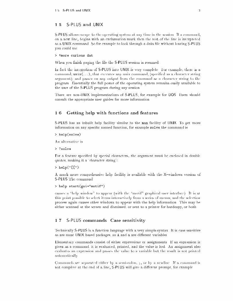
1.5 S-PLUS and UNIX
S-PLUS allows escape to the operating system at any time in the session. If a command,on a new line, begins with an exclamation mark then the rest of the line is interpretedas a UNIX command. So for example to look through a data �le without leaving S-PLUSyou could use
> !more curious.dat
When you �nish paging the �le the S-PLUS session is resumed.
In fact the integration of S-PLUS into UNIX is very complete. For example, there is acommand, unix(: : :), that executes any unix command, (speci�ed as a character stringargument), and passes on any output from the command as a character string to theprogram. Essentially the full power of the operating system remains easily available tothe user of the S-PLUS program during any session.
There are non-UNIX implementations of S-PLUS, for example for DOS. Users shouldconsult the appropriate user guides for more information.
1.6 Getting help with functions and features
S-PLUS has an inbuilt help facility similar to the man facility of UNIX. To get moreinformation on any speci�c named function, for example solve the command is
> help(solve)
An alternative is
> ?solve
For a feature speci�ed by special characters, the argument must be enclosed in doublequotes, making it a `character string':
> help("[[")
A much more comprehensive help facility is available with the X{windows version ofS-PLUS The command
> help.start(gui="motif")
causes a \help window" to appear (with the \motif" graphical user interface). It is atthis point possible to select items interactively from a series of menus, and the selectionprocess again causes other windows to appear with the help information. This may beeither scanned at the screen and dismissed, or sent to a printer for hardcopy, or both.
1.7 S-PLUS commands. Case sensitivity.
Technically S-PLUS is a function language with a very simple syntax. It is case sensitiveas are most UNIX based packages, so A and a are di�erent variables.
Elementary commands consist of either expressions or assignments. If an expression isgiven as a command, it is evaluated, printed, and the value is lost. An assignment alsoevaluates an expression and passes the value to a variable but the result is not printedautomatically.
Commands are separated either by a semi-colon, ;, or by a newline. If a command isnot complete at the end of a line, S-PLUS will give a di�erent prompt, for example
4 Introduction and Preliminaries
on second and subsequent lines and continue to read input until the command is syn-tactically complete. This prompt may also be changed if the user wishes. In these noteswe will generally omit the continuation prompt and indicate continuation by simpleindenting.
1.8 Recall and correction of previous commands
1.8.1 S-PLUS
S-PLUS (but not plain S) provides a mechanism for recall and correction of previouscommands. For interactive use this is a vital facility and greatly increases the productiveoutput of most people. To invoke S-PLUS with the command recall facility enabled usethe -e ag:
> Splus -e
Within the session, command recall is available using either emacs-style or vi-style com-mands. The former is very similar to command recall with an interactive shell suchas tcsh. Details are given in Appendix B of these notes, or they may be found in thereference manual or the online help documents.
1.8.2 Vanilla S
With S no built-in mechanism is available, but there are two common ways of obtainingcommand recall for interactive sessions.
� Run the S session under emacs using S{mode, a major mode designed to supportS. This is probably more convenient than even the inbuilt editor of S-PLUS in thelong term, however it does require a good deal of preliminary e�ort for persons notfamiliar with the emacs editor. It also often requires a dedicated workstation witha good deal of memory and other resources.
� Run the S session under some front end processor, such as the public domain fep
program, available from the public sources archives. This provides essentially thesame service as the inbuilt S-PLUS editor, but with somewhat more overhead, (buta great deal less overhead than emacs requires.)
1.9 Executing commands from, or diverting output to, a �le
If commands are stored on an external �le, say commands.S in the working directorywork, they may be executed at any time in an S-PLUS session with the command
> source("commands.S")
Similarly
> sink("record.lis")
will divert all subsequent output from the terminal to an external �le, record.lis. Thecommand
> sink()
restores it to the terminal once again.

1.10 Data directories. Permanency. Removing objects. 5
1.10 Data directories. Permanency. Removing objects.
All objects created during your S-PLUS sessions are stored, in a special form, in the.Data sub-directory of your working directory work, say.
Each object is held as a separate �le of the same name and so may be manipulated bythe usual UNIX commands such as rm, cp and mv. This means that if you resume yourS-PLUS session at a later time, objects created in previous sessions are still available,which is a highly convenient feature.
This also explains why it is recommended that you should use separate working directo-ries for di�erent jobs. Common names for objects are single letter names like x, y andso on, and if two problems share the same .Data sub-directory the objects will becomemixed up and you may overwrite one with another.
There is, however, another method of partitioning variables within the same .Data di-rectory using data frames. These are discussed further in x6.4.
In S-PLUS, to get a list of names of the objects currently de�ned use the command
> objects()
whose result is a vector of character strings giving the names.
When S-PLUS looks for an object, it searches in turn through a sequence of places knownas the search list. Usually the �rst entry in the search list is the .Data sub-directory ofthe current working directory. The names of the places currently on the search list aredisplayed by the function
> search()
The names of the objects held in any place in the search list can be displayed by givingthe objects() function an argument. For example
> objects(2)
lists the contents of the entity at position 2 of the search list. The search list can containeither data frames and allies, which are themselves internal S-PLUS objects, as well asdirectories of �les which are UNIX objects.
Extra entities can be added to this list with the attach() function and removed withthe detach() function, details of which can be found in the manual or the help facility.
To remove objects permanently the function rm is available:
> rm(x, y, z, ink, junk, temp, foo, bar)
The function remove() can be used to remove objects with non-standard names. Alsothe ordinary UNIX facility, rm, may be used to remove the appropriate �les in the .Datadirectory, as mentioned above.

6 Simple manipulations; numbers and vectors
2 Simple manipulations; numbers and vectors
2.1 Vectors
S-PLUS operates on named data structures. The simplest such structure is the vector,which is a single entity consisting of an ordered collection of numbers. To set up a vectornamed x, say, consisting of �ve numbers, namely 10:4, 5:6, 3:1, 6:4 and 21:7, use theS-PLUS command
> x <- c(10.4, 5.6, 3.1, 6.4, 21.7)
This is an assignment statement using the function c() which in this context can take anarbitrary number of vector arguments and whose value is a vector got by concatenatingits arguments end to end.1
A number occurring by itself in an expression is taken as a vector of length one.
Notice that the assignment operator is not the usual = operator, which is reserved foranother purpose. It consists of the two characters < (`less than') and - (`minus') occurringstrictly side-by-side and it `points' to the structure receiving the value of the expression.Assignments can also be made in the other direction, using the obvious change in theassignment operator. So the same assignment could be made using
> c(10.4, 5.6, 3.1, 6.4, 21.7) -> x
If an expression is used as a complete command, the value is printed and lost. So nowif we were to use the command
> 1/x
the reciprocals of the �ve values would be printed at the terminal (and the value of x,of course, unchanged).
The further assignment
> y <- c(x, 0, x)
would create a vector y with 11 entries consisting of two copies of x with a zero in themiddle place.
2.2 Vector arithmetic
Vectors can be used in arithmetic expressions, in which case the operations are performedelement by element. Vectors occurring in the same expression need not all be of the samelength. If they are not, the value of the expression is a vector with the same length asthe longest vector which occurs in the expression. Shorter vectors in the expressionare recycled as often as need be (perhaps fractionally) until they match the length ofthe longest vector. In particular a constant is simply repeated. So with the aboveassignments the command
> v <- 2*x + y + 1
generates a new vector v of length 11 constructed by adding together, element by element,2*x repeated 2:2 times, y repeated just once, and 1 repeated 11 times.
The elementary arithmetic operators are the usual +, -, *, / and ^ for raising to a power.In addition all of the common arithmetic functions are available. log, exp, sin, cos,tan, sqrt, and so on, all have their usual meaning. max and min select the largest andsmallest elements of an vector respectively. range is a function whose value is a vector
1With other than vector types of argument, such as list mode arguments, the action of c() is at
�rst sight rather di�erent. See x6.2.1.
2.3 Generating regular sequences 7
of length two, namely c(min(x), max(x)). length(x) is the number of elements in x,sum(x) gives the total of the elements in x and prod(x) their product.
Two statistical functions are mean(x) which calculates the sample mean, which is thesame as sum(x)/length(x), and var(x) which gives
sum((x-mean(x))^2)/(length(x)-1)
or sample variance. If the argument to var() is an n � p matrix the value is a p � p
sample covariance matrix got by regarding the rows as independent p�variate samplevectors.
sort(x) returns a vector of the same size as x with the elements arranged in increasingorder; however there are other more exible sorting facilities available (see order() orsort.list() which produce a permutation to do the sorting).
rnorm(x) is a function which generates a vector (or more generally an array) of pseudo-random standard normal deviates, of the same size as x.
2.3 Generating regular sequences
S-PLUS has a number of facilities for generating commonly used sequences of numbers.For example 1:30 is the vector c(1,2, : : :,29,30). The colon operator has highestpriority within an expression, so, for example 2*1:15 is the vector c(2,4,6, : : :,28,30).Put n <- 10 and compare the sequences 1:n-1 and 1:(n-1).
The construction 30:1 may be used to generate a sequence backwards.
The function seq() is a more general facility for generating sequences. It has �ve argu-ments, only some of which may be speci�ed in any one call. The �rst two arguments,if given, specify the beginning and end of the sequence, and if these are the only twoarguments given the result is the same as the colon operator. That is seq(2,10) is thesame vector as 2:10.
Parameters to seq(), and to many other S-PLUS functions, can also be given in namedform, in which case the order in which they appear is irrelevant. The �rst two parametersmay be named from=value and to=value; thus seq(1,30), seq(from=1, to=30) andseq(to=30, from=1) are all the same as 1:30. The next two parameters to seq() maybe named by=value and length=value, which specify a step size and a length for thesequence respectively. If neither of these is given, the default by=1 is assumed.
For example
> seq(-5, 5, by=.2) -> s3
generates in s3 the vector c(-5.0, -4.8, -4.6, : : :, 4.6, 4.8, 5.0). Similarly
> s4 <- seq(length=51, from=-5, by=.2)
generates the same vector in s4.
The �fth parameter may be named along=vector, which if used must be the only pa-rameter, and creates a sequence 1, 2, : : :, length(vector), or the empty sequence ifthe vector is empty (as it can be).
A related function is rep() which can be used for replicating a structure in variouscomplicated ways. The simplest form is
> s5 <- rep(x, times=5)
which will put �ve copies of x end-to-end in s5.

8 Simple manipulations; numbers and vectors
2.4 Logical vectors
As well as numerical vectors, S-PLUS allows manipulation of logical quantities. Theelements of a logical vectors have just two possible values, represented formally as F (for`false') and T (for `true').
Logical vectors are generated by conditions. For example
> temp <- x>13
sets temp as a vector of the same length as x with values F corresponding to elements ofx where the condition is not met and T where it is.
The logical operators are <, <=, >, >=, == for exact equality and != for inequality. Inaddition if c1 and c2 are logical expressions, then c1 & c1 is their intersection, c1 | c2 istheir union and ! c1 is the negation of c1.
Logical vectors may be used in ordinary arithmetic, in which case they are coerced intonumeric vectors, F becoming 0 and T becoming 1. However there are situations wherelogical vectors and their coerced numeric counterparts are not equivalent, for examplesee the next subsection.
2.5 Missing values
In some cases the components of a vector may not be completely known. When anelement or value is \not available" or a \missing value" in the statistical sense, a placewithin a vector may be reserved for it by assigning it the special value NA. In generalany operation on an NA becomes an NA. The motivation for this rule is simply that if thespeci�cation of an operation is incomplete, the result cannot be known and hence is notavailable.
The function is.na(x) gives a logical vector of the same size as x with value T if andonly if the corresponding element in x is NA.
> ind <- is.na(z)
Notice that the logical expression x == NA is quite di�erent from is.na(x) since NA isnot really a value but a marker for a quantity that is not available. Thus x == NA is avector of the same length as x all of whose values are NA as the logical expression itselfis incomplete and hence undecidable.
2.6 Character vectors
Character quantities and character vectors are used frequently in S-PLUS, for exampleas plot labels. Where needed they are denoted by a sequence of characters delimited bythe double quote character. E. g. "x-values", "New iteration results".
Character vectors may be concatenated into a vector by the c() function; examples oftheir use will emerge frequently.
The paste() function takes an arbitrary number of arguments and concatenates theminto a single character string. Any numbers given among the arguments are coercedinto character strings in the evident way, that is, in the same way they would be if theywere printed. The arguments are by default separated in the result by a single blankcharacter, but this can be changed by the named parameter, sep=string , which changesit to string , possibly empty.
For example
> labs <- paste(c("X","Y"), 1:10, sep="")
2.7 Index vectors. Selecting and modifying subsets of a data set 9
makes labs into the character vector
("X1", "Y2", "X3", "Y4", "X5", "Y6", "X7", "Y8", "X9", "Y10")
Note particularly that recycling of short lists takes place here too; thus c("X", "Y") isrepeated 5 times to match the sequence 1:10.
2.7 Index vectors. Selecting and modifying subsets of a data set
Subsets of the elements of a vector may be selected by appending to the name of thevector an index vector in square brackets. More generally any expression that evaluatesto a vector may have subsets of its elements similarly selected be appending an indexvector in square brackets immediately after the expression.
Such index vectors can be any of four distinct types.
1. A logical vector. In this case the index vector must be of the same length as thevector from which elements are to be selected. Values corresponding to T in theindex vector are selected and those corresponding to F omitted. For example
> y <- x[!is.na(x)]
creates (or re-creates) an object y which will contain the non-missing values of x,in the same order. Note that if x has missing values, y will be shorter than x. Also
> (x+1)[(!is.na(x)) & x>0] -> z
creates an object z and places in it the values of the vector x+1 for which thecorresponding value in x was both non-missing and positive.
2. A vector of positive integral quantities. In this case the values in the index vec-tor must lie in the the set f1, 2, : : :, length(x)g. The corresponding elementsof the vector are selected and concatenated, in that order, in the result. The indexvector can be of any length and the result is of the same length as the index vector.For example x[6] is the sixth component of x and
> x[1:10]
selects the �rst 10 elements of x, (assuming length(x) � 10). Also
> c("x","y")[rep(c(1,2,2,1), times=4)]
(an admittedly unlikely thing to do) produces a character vector of length 16consisting of "x", "y", "y", "x" repeated four times.
3. A vector of negative integral quantities. Such an index vector speci�es the val-ues to be excluded rather than included. Thus
> y <- x[-(1:5)]
gives y all but the �rst �ve elements of x.
4. A vector of character strings. This possibility only applies where an object hasa names attribute to identify its components. In this case a subvector of the namesvector may be used in the same way as the positive integral labels in 2. above.
> lunch <- fruit[c("apple","orange")]
This option is particularly useful in connection with data frames, as we shall seelater.
An indexed expression can also appear on the receiving end of an assignment, in whichcase the assignment operation is performed only on those elements of the vector. The

10 Simple manipulations; numbers and vectors
expression must be of the form vector[index vector] as having an arbitrary expressionin place of the vector name does not make much sense here.
The vector assigned must match the length of the index vector, and in the case of alogical index vector it must again be the same length as the vector it is indexing.
For example
> x[is.na(x)] <- 0
replaces any missing values in x by zeros and
> y[y<0] <- -y[y<0]
has the same e�ect as
> y <- abs(y)2
2Note that abs() does not work as expected with complex arguments. The appropriate function for
the complex modulus is Mod().

Objects, their modes and attributes 11
3 Objects, their modes and attributes
3.1 Intrinsic attributes: mode and length
The entities S-PLUS operates on are technically known as objects. Examples are vectorsof numeric (real) or complex values, vectors of logical values and vectors of characterstrings. These are known as `atomic' structures since their components are all of thesame type, or mode, namely numeric3, complex, logical and character respectively.
Vectors must have their values all of the same mode. Thus any given vector must beunambiguously either logical, numeric, complex or character. The only mild exceptionto this rule is the special \value" listed as NA for quantities not available. Note thata vector can be empty and still have a mode. For example the empty character stringvector is listed as character(0) and the empty numeric vector as numeric(0).
S-PLUS also operates on objects called lists, which are of mode list. These are orderedsequences of objects which individually can be of any mode. lists are known as `recursive'rather than atomic structures since their components can themselves be lists in their ownright.
The other recursive structures are those of mode function and expression. Functions
are the functions that form part of the S-PLUS system along with similar user writtenfunctions, which we discuss in some detail later in these notes. Expressions as objectsform an advanced part of S-PLUS which will not be discussed in these notes, exceptindirectly when we discuss formul� with we discuss modelling in S-PLUS.
By the mode of an object we mean the basic type of its fundamental constituents. Thisis a special case of an attribute of an object. The attributes of an object provide speci�cinformation about the object itself. Another attribute of every object is its length. Thefunctions mode(object) and length(object) can be used to �nd out the mode and lengthof any de�ned structure.
For example, if z is complex vector of length 100, then in an expression mode(z) is thecharacter string "complex" and length(z) is 100.
S-PLUS caters for changes of mode almost anywhere it could be considered sensible todo so, (and a few where it might not be). For example with
> z <- 0:9
we could put
> digits <- as.character(z)
after which digits is the character vector ("0", "1", "2", : : :, "9"). A furthercoercion, or change of mode, reconstructs the numerical vector again:
> d <- as.numeric(digits)
Now d and z are the same.4 There is a large collection of functions of the formas.something() for either coercion from one mode to another, or for investing an objectwith some other attribute it may not already posses. The reader should consult the help�le to become familiar with them.
3numeric mode is actually an amalgam of three distinct modes, namely integer, single precision anddouble precision, as explained in the manual.
4In general coercion from numeric to character and back again will not be exactly reversible, becauseof roundo� errors in the character representation.
12 Objects, their modes and attributes
3.2 Changing the length of an object
An \empty" object may still have a mode. For example
> e <- numeric()
makes e an empty vector structure of mode numeric. Similarly character() is a emptycharacter vector, and so on. Once an object of any size has been created, new componentsmay be added to it simply by giving it an index value outside its previous range. Thus
> e[3] <- 17
now makes e a vector of length 3, (the �rst two components of which are at this pointboth NA). This applies to any structure at all, provided the mode of the additionalcomponent(s) agrees with the mode of the object in the �rst place.
This automatic adjustment of lengths of an object is used often, for example in thescan() function for input.
Conversely to truncate the size of an object requires only an assignment to do so. Henceif alpha is a structure of length 10, then
> alpha <- alpha[2 * 1:5]
makes it an object of length 5 consisting of just the former components with even index.The old indices are not retained, of course.
3.3 attributes() and attr()
The function attributes(object) gives a list of all the non-intrinsic attributes currentlyde�ned for that object. The function attr(object,name) can be used to select a speci�cattribute. These functions are rarely used, except in rather special circumstances whensome new attribute is being created for some particular purpose, for example to associatea creation date or an operator with an S-PLUS object. The concept, however, is veryimportant.
3.4 The class of an object
A special attribute known as the class of the object has been introduced in the Au-gust 1991 release of S and S-PLUS to allow for an object oriented style of programming
in S-PLUS.
For example if an object has class data.frame, it will be printed in a certain way, theplot() function will display it graphically in a certain way, and other generic functionssuch as summary() will react to it as an argument in a way sensitive to its class.
To remove temporarily the e�ects of class, use the function unclass(). For example ifwinter has the class data.frame then
> winter
will print it in data frame form, which is rather like a matrix, whereas
> unclass(winter)
will print it as an ordinary list. Only in rather special situations do you need to use thisfacility, but one is when you are learning to come to terms with the idea of class andgeneric functions.
Generic functions and classes will be discussed further in x9.6, but only brie y.
Categories and factors 13
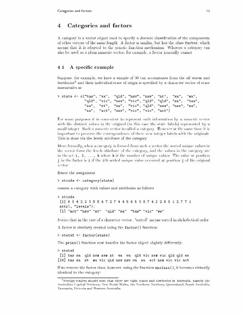
4 Categories and factors
A category is a vector object used to specify a discrete classi�cation of the componentsof other vectors of the same length. A factor is similar, but has the class factor, whichmeans that it is adapted to the generic function mechanism. Whereas a category canalso be used as a plain numeric vector, for example, a factor generally cannot.
4.1 A speci�c example
Suppose, for example, we have a sample of 30 tax accountants from the all states andterritories5 and their individual state of origin is speci�ed by a character vector of statemnemonics as
> state <- c("tas", "sa", "qld", "nsw", "nsw", "nt", "wa", "wa",
"qld", "vic", "nsw", "vic", "qld", "qld", "sa", "tas",
"sa", "nt", "wa", "vic", "qld", "nsw", "nsw", "wa",
"sa", "act", "nsw", "vic", "vic", "act")
For some purposes it is convenient to represent such information by a numeric vectorwith the distinct values in the original (in this case the state labels) represented by asmall integer. Such a numeric vector is called a category. However at the same time it isimportant to preserve the correspondence of these new integer labels with the originals.This is done via the levels attribute of the category.
More formally, when a category is formed from such a vector the sorted unique values inthe vector form the levels attribute of the category, and the values in the category arein the set 1, 2, : : :, k where k is the number of unique values. The value at positionj in the factor is i if the ith sorted unique value occurred at position j of the originalvector.
Hence the assignment
> stcode <- category(state)
creates a category with values and attributes as follows
> stcode
[1] 6 5 4 2 2 3 8 8 4 7 2 7 4 4 5 6 5 3 8 7 4 2 2 8 5 1 2 7 7 1
attr(, "levels"):
[1] "act" "nsw" "nt" "qld" "sa" "tas" "vic" "wa"
Notice that in the case of a character vector, \sorted" means sorted in alphabetical order.
A factor is similarly created using the factor() function:
> statef <- factor(state)
The print() function now handles the factor object slightly di�erently:
> statef
[1] tas sa qld nsw nsw nt wa wa qld vic nsw vic qld qld sa
[16] tas sa nt wa vic qld nsw nsw wa sa act nsw vic vic act
If we remove the factor class, however, using the function unclass(), it becomes virtuallyidentical to the category:
5Foreign readers should note that there are eight states and territories in Australia, namely theAustralian Capital Territory, New South Wales, the Northern Territory, Queensland, South Australia,
Tasmania, Victoria and Western Australia.

14 Categories and factors
> unclass(statef)
[1] 6 5 4 2 2 3 8 8 4 7 2 7 4 4 5 6 5 3 8 7 4 2 2 8 5 1 2 7 7 1
attr(, "levels"):
[1] "act" "nsw" "nt" "qld" "sa" "tas" "vic" "wa"
4.2 The function tapply() and ragged arrays
To continue the previous example, suppose we have the incomes of the same tax accoun-tants in another vector (in suitably large units of money)
> incomes <- c(60, 49, 40, 61, 64, 60, 59, 54, 62, 69, 70, 42, 56,
61, 61, 61, 58, 51, 48, 65, 49, 49, 41, 48, 52, 46,
59, 46, 58, 43)
To calculate the sample mean income for each state we can now use the special functiontapply():
> incmeans <- tapply(incomes, statef, mean)
giving a means vector with the components labelled by the levels
> incmeans
act nsw nt qld sa tas vic wa
44.5 57.333 55.5 53.6 55 60.5 56 52.25
The function tapply() is used to apply a function, here mean() to each group of compo-nents of the �rst argument, here incomes, de�ned by the levels of the second component,here statref as if they were separate vector structures. The result is a structure of thesame length as the levels attribute of the factor containing the results. The reader shouldconsult the help document for more details.
Suppose further we needed to calculate the standard errors of the state income means.To do this we need to write an S-PLUS function to calculate the standard error for anygiven vector. We discuss functions more fully later in these notes, but since there is anin built function var() to calculate the sample variance, such a function is a very simpleone liner, speci�ed by the assignment:
> stderr <- function(x) sqrt(var(x)/length(x))
(Writing functions will be considered later in x9.) After this assignment, the standarderrors are calculated by
> incster <- tapply(incomes, statef, stderr)
and the values calculated are then
> incster
act nsw nt qld sa tas vic wa
1.5 4.3102 4.5 4.1061 2.7386 0.5 5.244 2.6575
As an exercise you may care to �nd the usual 95% con�dence limits for the state meanincomes. To do this you could use tapply() once more with the length() functionto �nd the sample sizes, and the qt() function to �nd the percentage points of theappropriate t�distributions.
The function tapply() can be used to handle more complicated indexing of a vectorby multiple categories. For example, we might wish to split the tax accountants byboth state and sex. However in this simple instance what happens can be thought of asfollows. The values in the vector are collected into groups corresponding to the distinctentries in the category. The function is then applied to each of these groups individually.The value is a vector of function results, labelled by the levels attribute of the category.

4.2 The function tapply() and ragged arrays 15
The combination of a vector and a labelling factor or category is an example of what iscalled a ragged array, since the subclass sizes are possibly irregular. When the subclasssizes are all the same the indexing may be done implicitly and much more e�ciently, aswe see in the next section.
16 Arrays and matrices
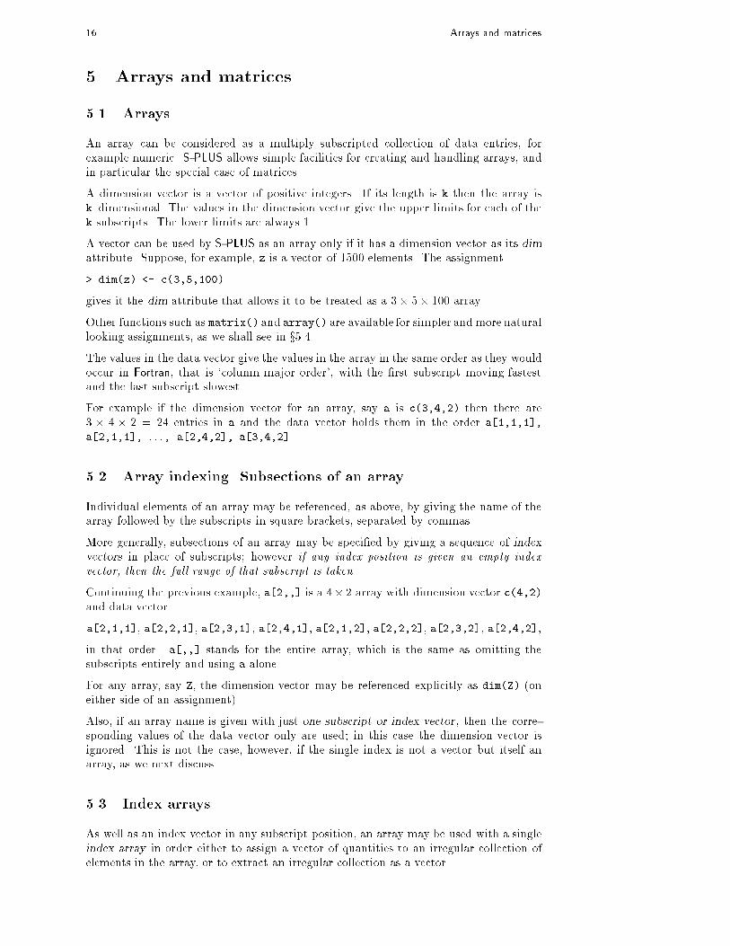
5 Arrays and matrices
5.1 Arrays
An array can be considered as a multiply subscripted collection of data entries, forexample numeric. S-PLUS allows simple facilities for creating and handling arrays, andin particular the special case of matrices.
A dimension vector is a vector of positive integers. If its length is k then the array isk{dimensional. The values in the dimension vector give the upper limits for each of thek subscripts. The lower limits are always 1.
A vector can be used by S-PLUS as an array only if it has a dimension vector as its dimattribute. Suppose, for example, z is a vector of 1500 elements. The assignment
> dim(z) <- c(3,5,100)
gives it the dim attribute that allows it to be treated as a 3� 5� 100 array.
Other functions such as matrix() and array() are available for simpler and more naturallooking assignments, as we shall see in x5.4.
The values in the data vector give the values in the array in the same order as they wouldoccur in Fortran, that is `column major order', with the �rst subscript moving fastestand the last subscript slowest.
For example if the dimension vector for an array, say a is c(3,4,2) then there are3 � 4 � 2 = 24 entries in a and the data vector holds them in the order a[1,1,1],
a[2,1,1], : : :, a[2,4,2], a[3,4,2].
5.2 Array indexing. Subsections of an array
Individual elements of an array may be referenced, as above, by giving the name of thearray followed by the subscripts in square brackets, separated by commas.
More generally, subsections of an array may be speci�ed by giving a sequence of indexvectors in place of subscripts; however if any index position is given an empty index
vector, then the full range of that subscript is taken.
Continuing the previous example, a[2,,] is a 4� 2 array with dimension vector c(4,2)and data vector
a[2,1,1], a[2,2,1], a[2,3,1], a[2,4,1], a[2,1,2], a[2,2,2], a[2,3,2], a[2,4,2],
in that order. a[,,] stands for the entire array, which is the same as omitting thesubscripts entirely and using a alone.
For any array, say Z, the dimension vector may be referenced explicitly as dim(Z) (oneither side of an assignment).
Also, if an array name is given with just one subscript or index vector, then the corre-sponding values of the data vector only are used; in this case the dimension vector isignored. This is not the case, however, if the single index is not a vector but itself anarray, as we next discuss.
5.3 Index arrays
As well as an index vector in any subscript position, an array may be used with a singleindex array in order either to assign a vector of quantities to an irregular collection ofelements in the array, or to extract an irregular collection as a vector.

5.3 Index arrays 17
A matrix example makes the process clear. In the case of a doubly indexed array, anindex matrix may be given consisting of two columns and as many rows as desired. Theentries in the index matrix are the row and column indices for the doubly indexed array.Suppose for example we have a 4� 5 array X and we wish to do the following:
� Extract elements X[1,3], X[2,2] and X[3,1] as a vector structure, and
� Replace these entries in the array X by 0s.
In this case we need a 3� 2 subscript array, as in the example given in Figure 1
> x <- array(1:20,dim=c(4,5)) # Generate a 4 x 5 array.
> x
[,1] [,2] [,3] [,4] [,5]
[1,] 1 5 9 13 17
[2,] 2 6 10 14 18
[3,] 3 7 11 15 19
[4,] 4 8 12 16 20
> i <- array(c(1:3,3:1),dim=c(3,2))
> i # i is a 3 x 2 index array.
[,1] [,2]
[1,] 1 3
[2,] 2 2
[3,] 3 1
> x[i] # Extract those elements
[1] 9 6 3
> x[i] <- 0 # Replace those elements by zeros.
> x
[,1] [,2] [,3] [,4] [,5]
[1,] 1 5 0 13 17
[2,] 2 0 10 14 18
[3,] 0 7 11 15 19
[4,] 4 8 12 16 20
>
Figure 1: Using an index array
As a less trivial example, suppose we wish to generate an (unreduced) design matrix fora block design de�ned by factors blocks (b levels) and varieties, (v levels). Furthersuppose there are n plots in the experiment. We could proceed as follows:
> Xb <- matrix(0, n, b)
> Xv <- matrix(0, n, v)
> ib <- cbind(1:n, blocks)
> iv <- cbind(1:n, varieties)
> Xb[ib] <- 1
> Xv[iv] <- 1
> X <- cbind(Xb, Xv)
Further, to construct the incidence matrix, N say, we could use
> N <- crossprod(Xb, Xv)
However a simpler direct way of producing this matrix is to use table():
> N <- table(blocks, varieties)

18 Arrays and matrices
5.4 The array() function
As well as giving a vector structure a dim attribute, arrays can be constructed fromvectors by the array function, which has the form
> Z <- array(data vector,dim vector)
For example, if the vector h contains 24, or fewer, numbers then the command
> Z <- array(h, dim=c(3,4,2))
would use h to set up 3� 4� 2 array in Z. If the size of h is exactly 24 the result is thesame as
> dim(Z) <- c(3,4,2)
However if h is shorter than 24, its values recycled from the beginning again to make itup to size 24. See x5.4.1 below. As an extreme but common example
> Z <- array(0, c(3,4,2)
makes Z an array of all zeros.
At this point dim(Z) stands for the dimension vector c(3,4,2), and Z[1:24] stands forthe data vector as it was in h, and Z[] with an empty subscript or Z with no subscriptstands for the entire array as an array.
Arrays may be used in arithmetic expressions and the result is an array formed by elementby element operations on the data vector. The dim attributes of operands generally needto be the same, and this becomes the dimension vector of the result. So if A, B and C areall similar arrays, then
> D <- 2*A*B + C + 1
makes D a similar array with data vector the result of the evident element by elementoperations. However the precise rule concerning mixed array and vector calculations hasto be considered a little more carefully.
5.4.1 Mixed vector and array arithmetic. The recycling rule
The precise rule a�ecting element by element mixed calculations with vectors and arraysis somewhat quirky and hard to �nd in the references. From experience I have found thefollowing to be a reliable guide.
� The expression is scanned from left to right.
� Any short vector operands are extended by recycling their values until they matchthe size of any previous (or subsequent) operands.
� As long as short vectors and arrays, only, are encountered, the arrays must all havethe same dim attribute or an error results.
� Any vector operand longer than some previous array immediately converts thecalculation to one in which all operands are coerced to vectors. A diagnosticmessage is issued if the size of the long vector is not a multiple of the (common)size of all previous arrays.
� If array structures are present and no error or coercion to vector has been precipi-tated, the result is an array structure with the common dim attribute of its arrayoperands,

5.5 The outer product of two arrays 19
5.5 The outer product of two arrays
An important operation on arrays is the outer product. If a and b are two numeric arrays,their outer product is an array whose dimension vector is got by concatenating their twodimension vectors, (order is important), and whose data vector is got by forming allpossible products of elements of the data vector of a with those of b. The outer productis formed by the special operator %o%:
> ab <- a %o% b
An alternative is
> ab <- outer(a, b, '*')
The multiplication function can be replaced by an arbitrary function of two variables.For example if we wished to evaluate the function
f(x; y) =cos(y)
1 + x2
over a regular grid of values with x� and y�coordinates de�ned by the S-PLUS vectorsx and y respectively, we could proceed as follows:
> f <- function(x,y) cos(y)/(1 + x^2)
> z <- outer(x, y, f)
In particular the outer product of two ordinary vectors is a doubly subscripted array(i.e. a matrix, of rank at most 1). Notice that the outer product operator is of coursenon-commutative.
5.5.1 An example: Determinants of 2� 2 digit matrices
As an arti�cial but cute example, consider the determinants of 2 � 2 matrices
�a b
c d
�
where each entry is a non-negative integer in the range 0; 1; : : : ; 9, that is a digit.
The problem is to �nd the determinants, ad � bc, of all possible matrices of this formand represent the frequency with which each value occurs as a high density plot. Thisamounts to �nding the probability distribution of the determinant if each digit is chosenindependently and uniformly at random.
A neat way of doing this uses the outer() function twice:
> d <- outer(0:9, 0:9)
> fr <- table(outer(d, d, "-"))
> plot(as.numeric(names(fr)), fr, type="h",
xlab="Determinant", ylab="Frequency")
Notice the coercion of the names attribute of the frequency table to numeric in order torecover the range of the determinant values. The \obvious" way of doing this problemwith for{loops, to be discussed in x8.2, is so ine�cient as to be impractical.
It is also perhaps surprising that about 1 in 20 such matrices is singular.
5.6 Generalized transpose of an array
The function aperm(a, perm) may be used to permute an array, a. The argumentperm must be a permutation of the integers f1, 2, : : :, kg, where k is the number ofsubscripts in a. The result of the function is an array of the same size as a but withold dimension given by perm[j] becoming the new jth dimension. The easiest way to
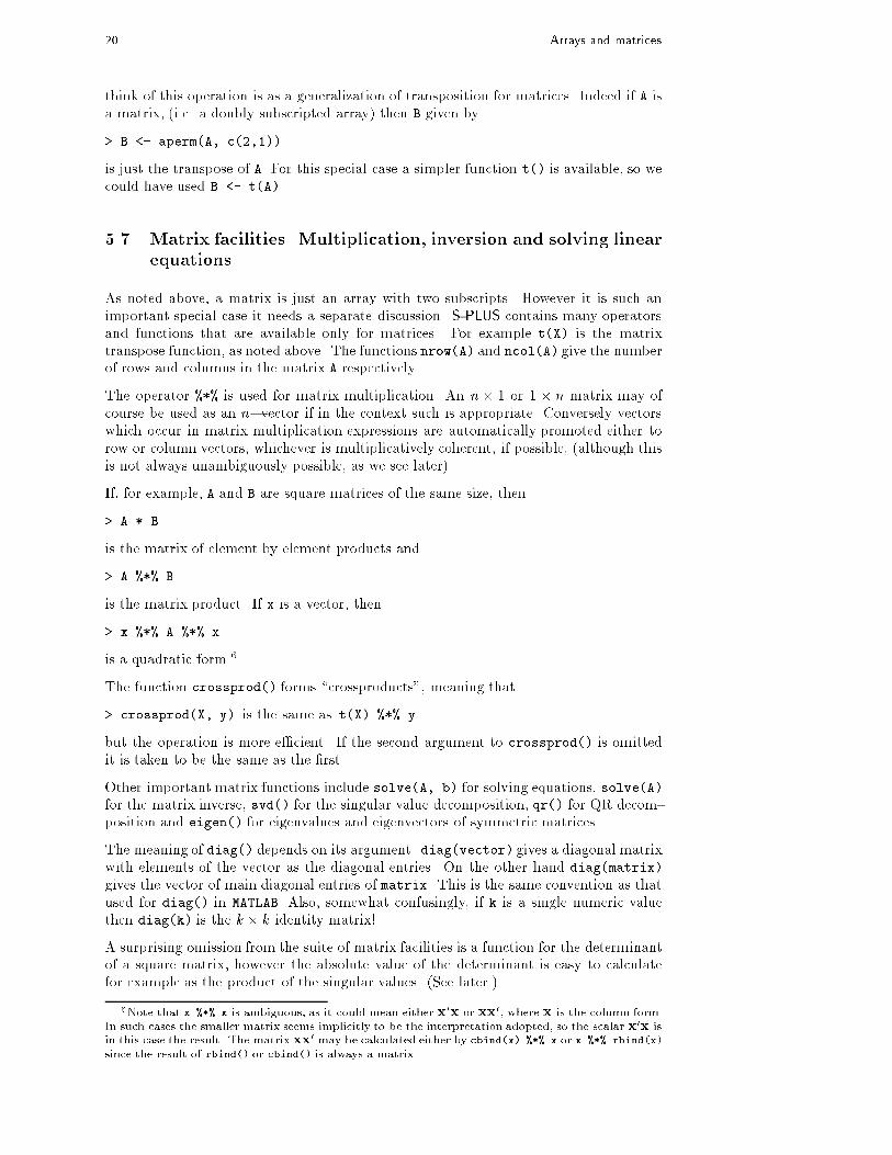
20 Arrays and matrices
think of this operation is as a generalization of transposition for matrices. Indeed if A isa matrix, (i.e. a doubly subscripted array) then B given by
> B <- aperm(A, c(2,1))
is just the transpose of A. For this special case a simpler function t() is available, so wecould have used B <- t(A).
5.7 Matrix facilities. Multiplication, inversion and solving linear
equations.
As noted above, a matrix is just an array with two subscripts. However it is such animportant special case it needs a separate discussion. S-PLUS contains many operatorsand functions that are available only for matrices. For example t(X) is the matrixtranspose function, as noted above. The functions nrow(A) and ncol(A) give the numberof rows and columns in the matrix A respectively.
The operator %*% is used for matrix multiplication. An n � 1 or 1 � n matrix may ofcourse be used as an n�vector if in the context such is appropriate. Conversely vectorswhich occur in matrix multiplication expressions are automatically promoted either torow or column vectors, whichever is multiplicatively coherent, if possible, (although thisis not always unambiguously possible, as we see later).
If, for example, A and B are square matrices of the same size, then
> A * B
is the matrix of element by element products and
> A %*% B
is the matrix product. If x is a vector, then
> x %*% A %*% x
is a quadratic form.6
The function crossprod() forms \crossproducts", meaning that
> crossprod(X, y) is the same as t(X) %*% y
but the operation is more e�cient. If the second argument to crossprod() is omittedit is taken to be the same as the �rst.
Other important matrix functions include solve(A, b) for solving equations, solve(A)for the matrix inverse, svd() for the singular value decomposition, qr() for QR decom-position and eigen() for eigenvalues and eigenvectors of symmetric matrices.
The meaning of diag() depends on its argument. diag(vector) gives a diagonal matrixwith elements of the vector as the diagonal entries. On the other hand diag(matrix)
gives the vector of main diagonal entries of matrix. This is the same convention as thatused for diag() in MATLAB. Also, somewhat confusingly, if k is a single numeric valuethen diag(k) is the k � k identity matrix!
A surprising omission from the suite of matrix facilities is a function for the determinantof a square matrix, however the absolute value of the determinant is easy to calculatefor example as the product of the singular values. (See later.)
6Note that x %*% x is ambiguous, as it could mean either x0x or xx0, where x is the column form.In such cases the smaller matrix seems implicitly to be the interpretation adopted, so the scalar x0x isin this case the result. The matrix xx0 may be calculated either by cbind(x) %*% x or x %*% rbind(x)
since the result of rbind() or cbind() is always a matrix.

5.8 Forming partitioned matrices. cbind() and rbind(). 21
5.8 Forming partitioned matrices. cbind() and rbind().
Matrices can be built up from given vectors and matrices by the functions cbind() andrbind(). Roughly cbind() forms matrices by binding together matrices horizontally, orcolumn-wise, and rbind() vertically, or row-wise.
In the assignment
> X <- cbind(arg1, arg2, arg3, : : :)
the arguments to cbind() must be either vectors of any length, or matrices with thesame column size, that is the same number of rows. The result is a matrix with theconcatenated arguments arg1, arg2, : : : forming the columns.
If some of the arguments to cbind() are vectors they may be shorter than the columnsize of any matrices present, in which case they are cyclically extended to match thematrix column size (or the length of the longest vector if no matrices are given).
The function rbind() does the corresponding operation for rows. In this case any vectorargument, possibly cyclically extended, are of course taken as row vectors.
Suppose X1 and X2 have the same number of rows. To combine these by columns into amatrix X, together with an initial column of 1s we can use
> X <- cbind(1, X1, X2)
The result of rbind() or cbind() always has matrix status. Hence cbind(x) andrbind(x) are possibly the simplest ways explicitly to allow the vector x to be treated asa column or row matrix respectively.
5.9 The concatenation function, c(), with arrays.
It should be noted that whereas cbind() and rbind() are concatenation functions thatrespect dim attributes, the basic c() function does not, but rather clears numeric objectsof all dim and dimnames attributes. This is occasionally useful in its own right.
The o�cial way to coerce an array back to a simple vector object is to use the functionas.vector()
> vec <- as.vector(X)
However a similar result can be achieved by using c() with just one argument, simplyfor this side-e�ect:
> vec <- c(X)
There are slight di�erences between the two, but ultimately the choice between them islargely a matter of style (with the former being preferable).
5.10 Frequency tables from factors. The table() function
Recall that a factor de�nes a partition into groups. Similarly a pair of factors de�nes atwo way cross classi�cation, and so on. The function table() allows frequency tables tobe calculated from equal length factors. If there are k category arguments, the result isa k�way array of frequencies.
Suppose, for example, that statef is a factor giving the state code for each entry in adata vector. The assignment
> statefr <- table(statef)

22 Arrays and matrices
gives in statefr a table of frequencies of each state in the sample. The frequencies areordered and labelled by the levels attribute of the category. This simple case is equivalentto, but more convenient than,
> statefr <- tapply(statef, statef, length)
Further suppose that incomef is a category giving a suitably de�ned \income class" foreach entry in the data vector, for example with the cut() function:
> factor(cut(incomes,breaks=35+10*(0:7))) -> incomef
Then to calculate a two-way table of frequencies:
> table(incomef,statef)
act nsw nt qld sa tas vic wa
35+ thru 45 1 1 0 1 0 0 1 0
45+ thru 55 1 1 1 1 2 0 1 3
55+ thru 65 0 3 1 3 2 2 2 1
65+ thru 75 0 1 0 0 0 0 1 0
Extension to higher way frequency tables is immediate.

Lists, data frames, and their uses 23
6 Lists, data frames, and their uses
6.1 Lists
An S-PLUS list is an object consisting of an ordered collection of objects known as itscomponents.
There is no particular need for the components to be of the same mode or type, and, forexample, a list could consist of a numeric vector, a logical value, a matrix, a complexvector, a character array, a function, and so on.
Components are always numbered and may always be referred to as such. Thus if Stis the name of a list with four components, these may be individually referred to asSt[[1]], St[[2]], St[[3]] and St[[4]]. If, further, St[[3]] is a triply subscriptedarray then St[[3]][1,1,1] is its �rst entry and dim(St[[3]]) is its dimension vector,and so on.
If St is a list, then the function length(St) gives the number of (top level) componentsit has.
Components of lists may also be named, and in this case the component may be referredto either by giving the component name as a character string in place of the number indouble square brackets, or, more conveniently, by giving an expression of the form
> name$component name
for the same thing.
This is a very useful convention as it makes it easier to get the right component ifyou forget the number. So if the components of St above had been named, and thenames were x, y, coefficients and covariance they could be referred to as St$y,St$covariance and so on, (or indeed as St[["y"]], St[["covariance"]] : : : but thisform is rarely if ever needed).
It is very important to distinguish St[[1]] from St[1]. \[[: : :]]" is the operator usedto select a single element, whereas \[: : :]" is a general subscripting operator. Thus theformer is the �rst object in the list St, and if it is a named list the name is not included.The latter is a sublist of the list St consisting of the �rst entry only. If it is a named list,
the name is transferred to the sublist.
The names of components may be abbreviated down to the minimum number of lettersneeded to identify them uniquely. Thus St$coefficients may be minimally speci�edas St$coe and St$covariance as St$cov.
The vector of names is in fact simply an attribute of the list like any other and maybe handled as such. Other structures besides lists may, of course, similarly be given anames attribute also.
6.2 Constructing and modifying lists
New lists may be formed from existing objects by the function list(). An assignmentof the form
> St <- list(name1=object1, name2=object2, : : :,namem=objectm)
sets up a list St of m components using comp1, : : : , compm for the components andgiving them names as speci�ed by the argument names, (which can be freely chosen). Ifthese names are omitted, the components are numbered only. The components used toform the list are copied when forming the new list and the originals are not a�ected.

24 Lists, data frames, and their uses
Lists, like any subscripted object, can be extended by specifying additional components.For example
> St[5] <- list(matrix=Mat)
6.2.1 Concatenating lists
When the concatenation function c() is given list arguments, the result is an objectof mode list also, whose components are those of the argument lists joined together insequence.
> list.ABC <- c(list.A, list.B, list.C)
Recall that with vector objects as arguments the concatenation function similarly joinedtogether all arguments into a single vector structure. In this case all other attributes,such as dim attributes, are discarded.
6.3 Some functions returning a list result
Functions and expressions in S-PLUS must return a single object as their result; in caseswhere the result has several component parts, the usual form is that of a list with namedcomponents.
6.3.1 Eigenvalues and eigenvectors
The function eigen(Sm) calculates the eigenvalues and eigenvectors of a symmetric ma-trix Sm. The result of this function is a list of two components named values andvectors. The assignment
> ev <- eigen(Sm)
will assign this list to ev. Then ev$val is the vector of eigenvalues of Sm and ev$vec isthe matrix of corresponding eigenvectors. Had we only needed the eigenvalues we couldhave used the assignment:
> evals <- eigen(Sm)$values
evals now holds the vector of eigenvalues and the second component is discarded. If the
expression
> eigen(Sm)
is used by itself as a command the two components are printed, with their names, at theterminal.
6.3.2 Singular value decomposition and determinants
The function svd(M) takes an arbitrary matrix argument, M, and calculates the singularvalue decomposition of M. This consists of a matrix of orthonormal columns U with thesame column space as M, a second matrix of orthonormal columns V whose column spaceis the row space of M and a diagonal matrix of positive entries D such that M = U %*%
D %*% t(V). D is actually returned as a vector of the diagonal elements. The result ofsvd(M) is actually a list of three components named d, u and v, with evident meanings.
If M is in fact square, then, it is not hard to see that
> absdetM <- prod(svd(M)$d)
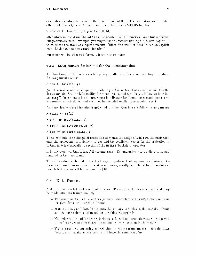
6.4 Data frames 25
calculates the absolute value of the determinant of M. If this calculation were neededoften with a variety of matrices it could be de�ned as an S-PLUS function
> absdet <- function(M) prod(svd(M)$d)
after which we could use absdet() as just another S-PLUS function. As a further trivialbut potentially useful example, you might like to consider writing a function, say tr(),to calculate the trace of a square matrix. [Hint: You will not need to use an explicitloop. Look again at the diag() function.]
Functions will be discussed formally later in these notes.
6.3.3 Least squares �tting and the QR decomposition
The function lsfit() returns a list giving results of a least squares �tting procedure.An assignment such as
> ans <- lsfit(X, y)
gives the results of a least squares �t where y is the vector of observations and X is thedesign matrix. See the help facility for more details, and also for the follow-up functionls.diag() for, among other things, regression diagnostics. Note that a grand mean termis automatically included and need not be included explicitly as a column of X.
Another closely related function is qr() and its allies. Consider the following assignments
> Xplus <- qr(X)
> b <- qr.coef(Xplus, y)
> fit <- qr.fitted(Xplus, y)
> res <- qr.resid(Xplus, y)
These compute the orthogonal projection of y onto the range of X in fit, the projectiononto the orthogonal complement in res and the coe�cient vector for the projection inb, that is, b is essentially the result of the MATLAB `backslash' operator.
It is not assumed that X has full column rank. Redundancies will be discovered andremoved as they are found.
This alternative is the older, low level way to perform least squares calculations. Al-though still useful in some contexts, it would now generally be replaced by the statisticalmodels features, as will be discussed in x10.
6.4 Data frames
A data frame is a list with class data.frame. There are restrictions on lists that maybe made into data frames, namely
� The components must be vectors (numeric, character, or logical), factors, numericmatrices, lists, or other data frames.
� Matrices, lists, and data frames provide as many variables to the new data frameas they have columns, elements, or variables, respectively.
� Numeric vectors and factors are included as is, and non-numeric vectors are coercedto be factors, whose levels are the unique values appearing in the vector.
� Vector structures appearing as variables of the data frame must all have the same
length, and matrix structures must all have the same row size.

26 Lists, data frames, and their uses
Data frames may in many ways be regarded as a matrix with columns possibly of di�eringmodes and attributes. It may be displayed in matrix form, and its rows and columnsextracted using matrix indexing conventions.
6.4.1 Making data frames
Objects satisfying the restrictions placed on the columns (components) of a data framemay be used to form one using the function data.frame:
> accountants <- data.frame(home=statef,loot=income, shot=incomef)
A list whose components conform to the restrictions of a data frame may be coerced intoa data frame using the function as.data.frame()
The simplest way to construct a data frame from scratch is to use the read.table()
function to read an entire data frame from an external �le. This is discussed further inx7.
6.4.2 attach() and detach()
The $ notation, such as accountants$statef, for list components is not always veryconvenient. A useful facility would be somehow to make the components of a list or dataframe temporarily visible as variables under their component name, without the need toquote the list name explicitly each time.
The attach() function, as well as having a directory name as its argument, may also havea data frame. Thus suppose lentils is a data frame with three variables lentils$u,lentils$v, lentils$w. The attach
> attach(lentils)
places the data frame in the search list at position 2, and provided there are no variablesu, v or w in position 1, u, v and w are available as variables from the data frame in theirown right. At this point an assignment such as
> u <- v+w
does not replace the component u of the data frame, but rather masks it with anothervariable u in the working directory at position 1 on the search list. To make a permanentchange to the data frame itself, the simplest way is to resort once again to the $ notation:
> lentils$u <- v+w
However the new value of component u is not visible until the data frame is detachedand attached again.
To detach a data frame, use the function
> detach()
More precisely, this statement detaches from the search list the entity currently at posi-tion 2. Thus in the present context the variables u, v and w would be no longer visible,except under the list notation as lentils$u and so on.
6.4.3 Working with data frames
A useful convention that allows you to work with many di�erent problems comfortablytogether in the same working directory is
6.4 Data frames 27
� gather together all variables for any well de�ned and separate problem in a dataframe under a suitably informative name;
� when working with a problem attach the appropriate data frame at position 2,and use the working directory at level 1 for operational quantities and temporaryvariables;
� before leaving a problem, add any variables you wish to keep for future referenceto the data frame using the $ form of assignment, and then detach();
� �nally remove all unwanted variables from the working directory and keep it aclean of left-over temporary variables as possible.
In this way it is quite simple to work with many problems in the same directory, all ofwhich have variables named x, y and z, for example.
6.4.4 Attaching arbitrary lists
attach() is a generic function that allows not only directories and data frames to beattached to the search list, but other classes of object as well. In particular any objectof mode list may be attached in the same way:
> attach(any.old.list)
It is also possible to attach objects of class pframe, to so-called parametrized data frames,needed for nonlinear regression and elsewhere.
Being a generic function it is also possible to add methods for attaching yet more classesof object should the need arise.
28 Reading data from �les
7 Reading data from �les
Large data objects will usually be read as values from external �les rather than enteredduring an S-PLUS session at the keyboard. This is done most conveniently with thescan() function for simple data items, and the read.table() function for reading entiredata frames directly.
7.1 The scan() function
Suppose the data vectors are of equal length and are to be read in in parallel. Furthersuppose that there are three vectors, the �rst of mode character and the remaining twoof mode numeric, and the �le is input.dat. The �rst step is to use scan() to read inthe three vectors as a list, as follows
> in <- scan("input.dat", list("",0,0))
The second argument is a dummy list structure that establishes the mode of the threevectors to be read. The result, held in in, is a list whose components are the threevectors read in. To separate the data items into three separate vectors, use assignmentslike
> label <- in[[1]]; x <- in[[2]]; y <- in[[3]]
More conveniently, the dummy list can have named components, in which case the namescan be used to access the vectors read in. For example
> in <- scan("input.dat", list(id="", x=0, y=0))
If you wish to access the variables separately they may either be re-assigned to variablesin the working frame:
> label <- in$id; x <- in$x; y <- in$y
or the list may be attached at position 2 of the search list, (see x6.4.4).
If the second argument is a single value and not a list, a single vector is read in, allcomponents of which must be of the same mode as the dummy value.
> X <- matrix(scan("light.dat", 0), ncol=5, byrow=T)
There are more elaborate input facilities available and these are detailed in the manual.
7.2 The read.table() function
To read an entire data frame directly, the external �le must have a special form.
� The �rst line of the �le should have have a name for each variable in the dataframe.
� Each additional line of the �le has its �rst item a row label and the values for eachvariable.
If the �le has one fewer item in its �rst line than in its second, this arrangement ispresumed to be in force. So the �rst few lines of a �le to be read as a data frame mightlook as in Figure 2. By default numeric items (except row labels) are read as numericvariables and non-numeric variables, such as Cent.heat in the example, as factors. Thiscan be changed if necessary.
The function read.table() can then be used to read the data frame directly
> HousePrice <- read.table("houses.data")
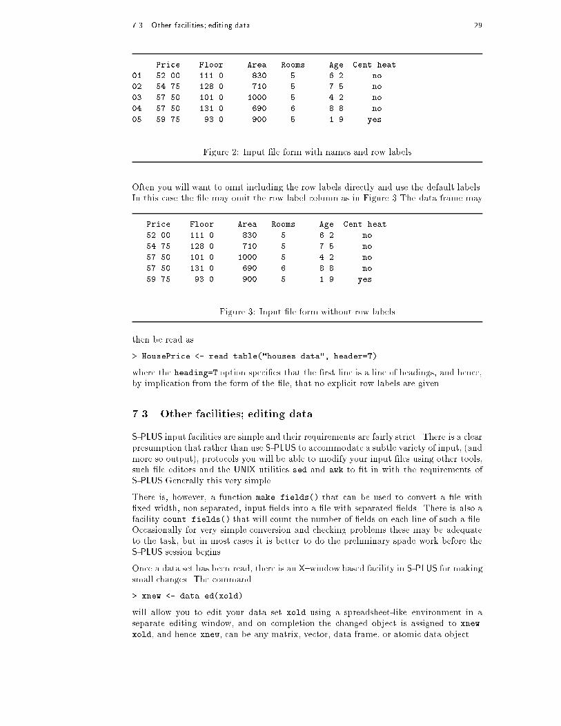
7.3 Other facilities; editing data 29
Price Floor Area Rooms Age Cent.heat
01 52.00 111.0 830 5 6.2 no
02 54.75 128.0 710 5 7.5 no
03 57.50 101.0 1000 5 4.2 no
04 57.50 131.0 690 6 8.8 no
05 59.75 93.0 900 5 1.9 yes
...
Figure 2: Input �le form with names and row labels
Often you will want to omit including the row labels directly and use the default labels.In this case the �le may omit the row label column as in Figure 3 The data frame may
Price Floor Area Rooms Age Cent.heat
52.00 111.0 830 5 6.2 no
54.75 128.0 710 5 7.5 no
57.50 101.0 1000 5 4.2 no
57.50 131.0 690 6 8.8 no
59.75 93.0 900 5 1.9 yes
...
Figure 3: Input �le form without row labels
then be read as
> HousePrice <- read.table("houses.data", header=T)
where the heading=T option speci�es that the �rst line is a line of headings, and hence,by implication from the form of the �le, that no explicit row labels are given.
7.3 Other facilities; editing data
S-PLUS input facilities are simple and their requirements are fairly strict. There is a clearpresumption that rather than use S-PLUS to accommodate a subtle variety of input, (andmore so output), protocols you will be able to modify your input �les using other tools,such �le editors and the UNIX utilities sed and awk to �t in with the requirements ofS-PLUS Generally this very simple.
There is, however, a function make.fields() that can be used to convert a �le with�xed width, non separated, input �elds into a �le with separated �elds. There is also afacility count.fields() that will count the number of �elds on each line of such a �le.Occasionally for very simple conversion and checking problems these may be adequateto the task, but in most cases it is better to do the preliminary spade work before theS-PLUS session begins.
Once a data set has been read, there is an X{window based facility in S-PLUS for makingsmall changes. The command
> xnew <- data.ed(xold)
will allow you to edit your data set xold using a spreadsheet-like environment in aseparate editing window, and on completion the changed object is assigned to xnew.xold, and hence xnew, can be any matrix, vector, data frame, or atomic data object.
30 More language features. Loops and conditional execution
8 More language features. Loops and conditional
execution
8.1 Grouped expressions
S-PLUS is an expression language in the sense that its only command type is a functionor expression which returns a result. Even an assignment is an expression whose resultis the value assigned, and it may be used wherever any expression may be used; inparticular multiple assignments are possible.
Commands may be grouped together in braces, {expr1; expr2;: : :; exprm}, in whichcase the value of the group is the result of the last expression in the group evaluated. Sincesuch a group is also an expression it may, for example, be itself included in parenthesesand used a part of an even larger expression, and so on.
8.2 Control statements
The language has available a conditional construction of the form
> if (expr1) expr2 else expr3
where expr1 must evaluate to a logical value and the result of the entire expression isthen evident.
There is also a for{loop construction which has the form
> for (name in expr1) expr2
where name is the loop variable. expr1 is a vector expression, (often a sequence like1:20), and expr2 is often a grouped expression with its sub-expressions written in termsof the dummy name. expr2 is repeatedly evaluated as name ranges through the valuesin the vector result of expr1.
As an example, suppose ind is a vector of class indicators and we wish to produceseparate plots of y versus x within classes. One possibility here is to use coplot() to bediscussed later, which will produce an array of plots corresponding to each level of thefactor. Another way to do this, now putting all plots on the one display, is as follows:
> yc <- split(y, ind); xc <- split(x, ind)
> for (i in 1:length(yc)){plot(xc[[i]], yc[[i]]);
abline(lsfit(xc[[i]], yc[[i]]))}
(Note the function split() which produces a list of vectors got by splitting a largervector according to the classes speci�ed by a category. This is a useful function, mostlyused in connection with boxplots. See the help facility for further details.)
Other looping facilities include the
> repeat expr
statement and the
> while (condition) expr
statement. The break statement can be used to terminate any loop abnormally, andnext can be used to discontinue one particular cycle.
Control statements are most often used in connection with functions which are discussedin x9, and where more examples will emerge.

Writing your own functions 31
9 Writing your own functions
As we have seen informally along the way, the S-PLUS language allows the user to createobjects of mode function. These are true S-PLUS functions that are stored in a specialinternal form and may be used in further expressions and so on. In the process thelanguage gains enormously in power, convenience and elegance, and learning to writeuseful functions is one of the main ways to make your use of S-PLUS comfortable andproductive.
It should be emphasized that most of the functions supplied as part of the S-PLUS system,such as mean(), var(), postscript() and so on, are themselves written in S-PLUS andthus do not di�er materially from user written functions.
A function is de�ned by an assignment of the form
> name <- function(arg1, arg2, : : :) expression
The expression is an S-PLUS expression, (usually a grouped expression), that uses thearguments, argi, to calculate a value. The value of the expression is the value returnedfor the function.
A call to the function then usually takes the form name(expr1, expr2, : : :) and mayoccur anywhere a function call is legitimate.
For example, consider a function to emulate directly the MATLAB backslash command,which returns the coe�cients of the orthogonal projection of the vector y onto the columnspace of the matrix, X. Thus given a vector yn�1 and a matrix Xn�p then
Xny =def: (X0X)�X0y
where (X0X)� is a generalized inverse of X0X.
> bslash <- function(X, y)
{
X <- qr(X)
qr.coef(X, y)
}
After this object is created it is permanent, like all objects, and may be used in statementssuch as
> regcoeff <- bslash(Design, yvar)
and so on.
The classical S-PLUS function lsfit() does this job quite well, and more. It in turnuses the functions qr() and qr.coef() in the slightly counterintuitive way above to dothis part of the calculation. Hence there is probably some value in having just this partisolated in a simple to use function if it is going to be in frequent use. If so, we may wishto make it a matrix binary operator for even more convenient use.
9.1 De�ning new binary operators.
Had we given the bslash() function a di�erent name, namely one of the form
%anything%
it could have been used as a binary operator in expressions rather than in function form.Suppose, for example, we choose ! for the internal character. The function de�nitionwould then start as
> "%!%" <- function(X, y) {: : : }

32 Writing your own functions
(Note the use of quote marks.) The function could then be used as X %!% y. (Thebackslash symbol itself is not a convenient choice as it presents special problems in thiscontext.)
The matrix multiplication operator, %*%, and the outer product matrix operator %o% areother examples of binary operators de�ned in this way.
9.2 Named arguments and defaults. \: : :"
As �rst noted in x2.3 if arguments to called functions are given in the \name=object"form, they may be given in any order. Furthermore the argument sequence may beginin the unnamed, positional form, and specify named arguments after the positionalarguments.
Thus if there is a function fun1 de�ned by
> fun1 <- function(data, data.frame, graph, limit) {: : : 7}
Then the function may be invoked in several ways, for example
> ans <- fun1(d, df, 20, T)
> ans <- fun1(d, df, graph=T, limit=20)
> ans <- fun1(data=d, limit=20, graph=T, data.frame=df)
are all equivalent.
In many cases arguments can be given commonly appropriate default values, in whichcase they may be omitted altogether from the call when the defaults are appropriate.For example, if fun1 were de�ned as
> fun1 <- function(data, data.frame, graph=T, limit=20) {: : : 7}
it could be called as
> ans <- fun1(d, df)
which is now equivalent to the three cases above, or as
> ans <- fun1(d, df, limit=10)
which changes one of the defaults.
It is important to note that defaults may be arbitrary expressions, even involving otherarguments to the same function; they are not restricted to be constants as in our simpleexample here.
Another frequent requirement is to allow one function to pass on argument settings toanother. For example many graphics functions use the function par() and functions likeplot() allow the user to pass on graphical parameters to par() to control the graphicaloutput. This can be done by including an extra argument, literally \: : :", of the function,which may then be passed on. An outline example is given in Figure 4. Note here thatthe ellipses, \: : :" are literal S-PLUS, not a typographical device.
9.3 Assignments within functions are local. Frames.
Note that any ordinary assignments done within the function are local and temporary
and lost after exit from the function. Thus the assignment X <- qr(X) does not a�ectthe value of the argument in the calling program.
7This ellipsis is used as a customary typographical device to mean an abridgement. This is not thecase in the latter part of section.

9.4 More advanced examples 33
fun1 <- function(data, data.frame, graph=T, limit=20, ...)
{
[omitted statements]
if (graph)
par(pch="*", ...)
[more omissions]
}
Figure 4: Use of the ellipsis argument, \: : :"
To understand completely the rules governing the scope of S-PLUS assignments thereader needs to be familiar with the notion of an evaluation frame. This is a somewhatadvanced, though hardly di�cult, topic and is not covered further in these notes.
If global and permanent assignments are intended within a function, then the `superas-signment' operator, `<<-' can be used. See the help document for details, and also seethe synchronize() function.
9.4 More advanced examples
E�ciency factors in block designs
As a more complete, if a little pedestrian, example of a function, consider �nding thee�ciency factors for a block design. (Some aspects of this problem have already beendiscussed in x5.3.)
A block design is de�ned by two factor, say blocks (b levels) and varieties, (v levels).If Rv�v and Kb�b are the replications and block size matrices, and N b�v is the incidencematrix, then the e�ciency factors are de�ned as the eigenvalues of the matrix
E = Iv � R�1=2N 0K�1NR�1=2 = Iv � A0A
where A = K�1=2NR�1=2. One way to write the function is as in Figure 5.
> bdeff <- function(blocks, varieties) {
blocks <- as.factor(blocks) # minor safety move
b <- length(levels(blocks))
varieties <- as.factor(varieties) # minor safety move
v <- length(levels(varieties))
K <- as.vector(table(blocks)) # remove dim attr
R <- as.vector(table(varieties)) # remove dim attr
N <- table(blocks, varieties)
A <- 1/sqrt(K) * N * rep(1/sqrt(R), rep(b, v))
sv <- svd(A)
list(eff=1 - sv$d^2, blockcv=sv$u, varietycv=sv$v)
}
Figure 5: A function for block design e�ciencies
It is numerically slightly better to work with the singular value decomposition on thisoccasion rather than the eigenvalue routines.
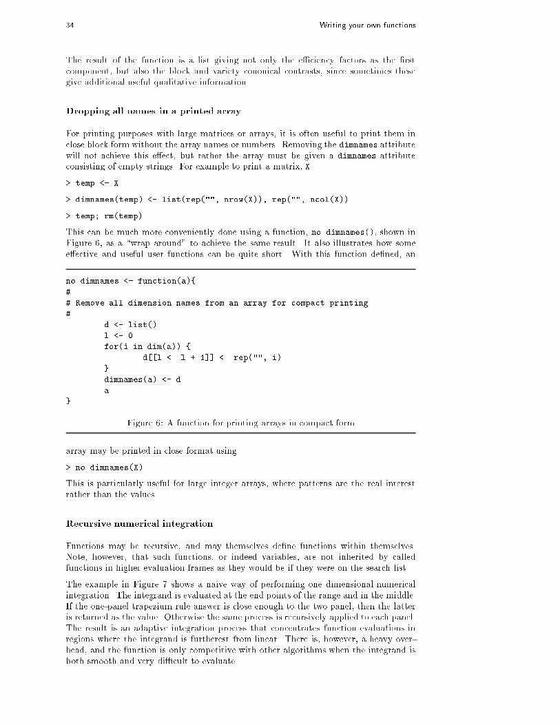
34 Writing your own functions
The result of the function is a list giving not only the e�ciency factors as the �rstcomponent, but also the block and variety cononical contrasts, since sometimes thesegive additional useful qualitative information.
Dropping all names in a printed array
For printing purposes with large matrices or arrays, it is often useful to print them inclose block form without the array names or numbers. Removing the dimnames attributewill not achieve this e�ect, but rather the array must be given a dimnames attributeconsisting of empty strings. For example to print a matrix, X
> temp <- X
> dimnames(temp) <- list(rep("", nrow(X)), rep("", ncol(X))
> temp; rm(temp)
This can be much more conveniently done using a function, no.dimnames(), shown inFigure 6, as a \wrap around" to achieve the same result. It also illustrates how somee�ective and useful user functions can be quite short. With this function de�ned, an
no.dimnames <- function(a){
#
# Remove all dimension names from an array for compact printing.
#
d <- list()
l <- 0
for(i in dim(a)) {
d[[l <- l + 1]] <- rep("", i)
}
dimnames(a) <- d
a
}
Figure 6: A function for printing arrays in compact form
array may be printed in close format using
> no.dimnames(X)
This is particularly useful for large integer arrays, where patterns are the real interestrather than the values.
Recursive numerical integration
Functions may be recursive, and may themselves de�ne functions within themselves.Note, however, that such functions, or indeed variables, are not inherited by calledfunctions in higher evaluation frames as they would be if they were on the search list.
The example in Figure 7 shows a naive way of performing one dimensional numericalintegration. The integrand is evaluated at the end points of the range and in the middle.If the one-panel trapezium rule answer is close enough to the two panel, then the latteris returned as the value. Otherwise the same process is recursively applied to each panel.The result is an adaptive integration process that concentrates function evaluations inregions where the integrand is furtherest from linear. There is, however, a heavy over-head, and the function is only competitive with other algorithms when the integrand isboth smooth and very di�cult to evaluate.

9.5 Customizing the environment. .First and .Last 35
The example is also given partly as a little puzzle in S-PLUS programming.
area <- function(f, a, b, eps = 1.0e-06, lim = 10)
{
fun1 <- function(f, a, b, fa, fb, a0, eps, lim, fun)
{
d <- (a + b)/2
h <- (b - a)/4
fd <- f(d)
a1 <- h * (fa + fd)
a2 <- h * (fd + fb)
if(abs(a0 - a1 - a2) < eps || lim == 0)
return(a1 + a2)
else {
return(fun(f, a, d, fa, fd, a1, eps, lim - 1, fun) +
fun(f, d, b, fd, fb, a2, eps, lim - 1, fun))
}
}
fa <- f(a)
fb <- f(b)
a0 <- ((fa + fb) * (b - a))/2
fun1(f, a, b, fa, fb, a0, eps, lim, fun1)
}
Figure 7: A recursive function within a function
9.5 Customizing the environment. .First and .Last
Any function named .First() in the .Data directory has a special status. It is automat-ically performed at the beginning of an S-PLUS session and may be used to initialize theenvironment. For example, the de�nition in Figure 8 alters the prompt to $ and sets upvarious other useful things that can then be taken for granted in the rest of the session.Similarly a function .Last(), if de�ned, is executed at the very end of the session. An
> .First <- function() {
options(prompt="$ ", continue="+\t") # $ is the prompt
options(digits=5, length=999) # custom numbers and printout
options(gui="motif") # default graphics user interface
tek4014() # for terminal work
par(pch = "+") # plotting character
attach(paste(unix("echo $HOME"), "/.Data", sep = ""))
# Home of my personal library
library(examples) # attach also the system examples
}
Figure 8: An example of a .First() function
example is given in Figure 9

36 Writing your own functions
> .Last <- function() {
graphics.off() # a small safety measure.
cat(paste(unix("date"),"\nAdios\n")) # Is it time for lunch?
}
Figure 9: An example of a .Last() function
9.6 Classes, generic functions and object orientation
The class of an object determines how it will be treated by what are known as genericfunctions. Put the other way round, a generic function performs a task or action on itsarguments speci�c to the class of the argument itself. If the argument lacks any classattribute, or has a class not catered for speci�cally by the generic function in question,there is always a default action provided.
An example makes things clearer. In a sense the print() function has always beengeneric, since its action is to adopt a style of output appropriate to its arguments. Thusa matrix appears as a matrix, a vector as a vector, and so on. (Note that the print()function can be called explicitly, or implicitly by giving an expression as a completecommand.)
The August 1991 release of S-PLUS increases the number of such functions, alters themechanism by which they are implemented and via the class mechanism o�ers the userthe facility of designing and writing generic functions for special purposes. Among theother new, or newly generic functions are plot() for displaying objects graphically,summary() for summarising analyses of various types, and anova() for comparing sta-tistical models.
The number of generic functions that can treat a class in a speci�c way can be quitelarge. For example, the functions that can accommodate in some fashion objects of classdata.frame include
[, [[<-, dbdetach, dimnames<-, pairs, signif,
[<-, aperm, dim, formula, plot, summary,
[[, atan, dimnames, ordered<-, print, t,
A currently complete list can be got by using the methods() function:
> methods(class="data.frame")
Conversely the number of classes a generic function can handle can also be quite large.For example the plot() function has variants for classes of object
data.frame, default, glm, pregam, surv.fit,
design, factor, lm, preloess, tree,
formula, gam, loess, profile, tree.sequence,
and perhaps more. A complete list can be got again by using the methods() function:
> methods(plot)
The reader is referred to the o�cial references for a complete discussion of this mecha-nism.
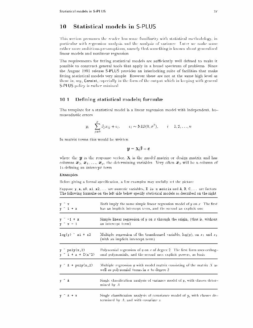
Statistical models in S-PLUS 37
10 Statistical models in S-PLUS
This section presumes the reader has some familiarity with statistical methodology, inparticular with regression analysis and the analysis of variance. Later we make somerather more ambitious presumptions, namely that something is known about generalizedlinear models and nonlinear regression.
The requirements for �tting statistical models are su�ciently well de�ned to make itpossible to construct general tools that apply in a broad spectrum of problems. Sincethe August 1991 release S-PLUS provides an interlocking suite of facilities that make�tting statistical models very simple. However these are not at the same high level asthose in, say, Genstat, especially in the form of the output which in keeping with generalS-PLUS policy is rather minimal.
10.1 De�ning statistical models; formul�
The template for a statistical model is a linear regression model with independent, ho-moscedastic errors
yi =
pXj=0
�jxij + ei; ei � NID(0; �2); i = 1; 2; : : :; n
In matrix terms this would be written
y = X� + e
where the y is the response vector, X is the model matrix or design matrix and hascolumns x0, x1, : : :, xp, the determining variables. Very often x0 will be a column of1s de�ning an intercept term.
Examples.
Before giving a formal speci�cation, a few examples may usefully set the picture.
Suppose y, x, x0, x1, x2, : : : are numeric variables, X is a matrix and A, B, C, : : : are factors.
The following formul� on the left side below specify statistical models as described on the right.
y ~ x
y ~ 1 + x
Both imply the same simple linear regression model of y on x. The �rst
has an implicit intercept term, and the second an explicit one.
y ~ -1 + x
y ~ x - 1
Simple linear regression of y on x through the origin, (that is, without
an intercept term).
log(y) ~ x1 + x2 Multiple regression of the transformed variable, log(y), on x1 and x2
(with an implicit intercept term).
y ~ poly(x,2)
y ~ 1 + x + I(x^2)
Polynomial regression of y on x of degree 2. The �rst form uses orthog-
onal polynomials, and the second uses explicit powers, as basis.
y ~ X + poly(x,2) Multiple regression y with model matrix consisting of the matrix X as
well as polynomial terms in x to degree 2.
y ~ A Single classi�cation analysis of variance model of y, with classes deter-
mined by A.
y ~ A + x Single classi�cation analysis of covariance model of y, with classes de-
termined by A, and with covariate x.

38 Statistical models in S-PLUS
y ~ A*B
y ~ A + B + A:B
y ~ B %in% A
y ~ A/B
Two factor non-additive model of y on A and B. The �rst two specify
the same crossed classi�cation and the second two specify the same
nested classi�cation. In abstract terms all four specify the same modelsubspace.
y ~ (A + B + C)^2
y ~ A*B*C - A:B:C
Three factor experiment but with a model containing main e�ects andtwo factor interactions only. Both formul� specify the same model.
y ~ A * x
y ~ A/x
y ~ A/(1 + x) - 1
Separate simple linear regression models of y on x within the levels ofA, with di�erent codings. The last form produces explicit estimates of
as many di�erent intercepts and slopes as there are levels in A.
y ~ A*B + Error(C) An experiment with two treatment factors, A and B, and error strata
determined by factor C. For example a split plot experiment, withwhole plots, (and hence also subplots), determined by factor C.
The operator ~ is used to de�ne a model formula in S-PLUS. The form, for an ordinarylinear model, is
response ~ [�] term1 � term2 � term3 � � � �
response is a vector or matrix, (or expression evaluating to a vector or matrix) de�ningthe response variable(s).
� is an operator, either + or -, implying the inclusion or exclusion of a term in themodel, (the �rst is optional).
term is either
� a vector or matrix expression, or 1,
� a factor, or
� a formula expression consisting of factors, vectors or matrices connected byformula operators.
In all cases each term de�nes a collection of columns either to be added to orremoved from the model matrix. A 1 stands for an intercept column and is bydefault included in the model matrix unless explicitly removed.
The formula operators are similar in e�ect to the Wilkinson and Rogers notation usedused by such programs a Glim and Genstat. One inevitable change is that the operator\." becomes \:" since the period is a valid name character in S-PLUS. The notation issummarised as in the Table 1 (based on Chambers & Hastie, p. 29).
Note that inside the parentheses that usually enclose function arguments all operatorshave their normal arithmetic meaning. The function I() is an identity function usedonly to allow terms in model formul� to be de�ned using arithmetic operators.
Note particularly that the model formul� specify the columns of the model matrix, spec-i�cation of the parameters is implicit. This is not the case in other contexts, for examplein �tting nonlinear models
10.2 Regression models; �tted model objects
The basic function for �tting ordinary multiple models is lm(), and a streamlined versionof the call is as follows:
> �tted.model <- lm(formula, data=data.frame)

10.3 Generic functions for extracting information 39
Form Meaning
Y ~ M Y is modelled as M
M1 + M2 Include M1 and M2
M1 - M2 Include M1 leaving out terms of M2
M1:M2 The tensor product of M1 and M2. If both terms factors, then the\subclasses" factor.
M1 %in% M2 Similar to M1:M2, but with a di�erent coding.
M1*M2 M1 + M2 + M1:M2
M1/M2 M1 + M2 %in% M1
M^n All terms in M together with \interactions" up to order n
I(M) Insulate M . Inside M all operators have their normal arithmeticmeaning, and that term appears in the model matrix.
Table 1: Summary of model operator semantics
For example
> fm2 <- lm(y ~ x1 + x2, data=production)
would �t a multiple regression model of y on x1 and x2 (with implicit intercept term).
The important but technically optional parameter data=production speci�es that anyvariables needed to construct the model should come �rst from the production data
frame. This is the case regardless of whether data frame production has been attached
to the search list or not.
10.3 Generic functions for extracting information
The value of lm() is �tted model object; technically a list of results of class lm. Infor-mation about the �tted model can then be displayed, extracted, plotted and so on byusing generic functions that orient themselves to objects of class lm. A full list of these
at the present time is
add1 coef effects kappa predict residuals
alias deviance family labels print summary
anova drop1 formula plot proj
A brief description of the most commonly used ones is given in Table 2.
10.4 Analysis of variance; comparing models
The model �tting function aov(formula, data=data.frame) operates at the simplestlevel in a very similar way to the function lm(), and most of the generic functions listedin Table 2 apply.
It should be noted that in addition aov() allows an analysis of models with multipleerror strata such as split plot experiments, or balanced incomplete block designs withrecovery of inter-block information envisaged. Model formula
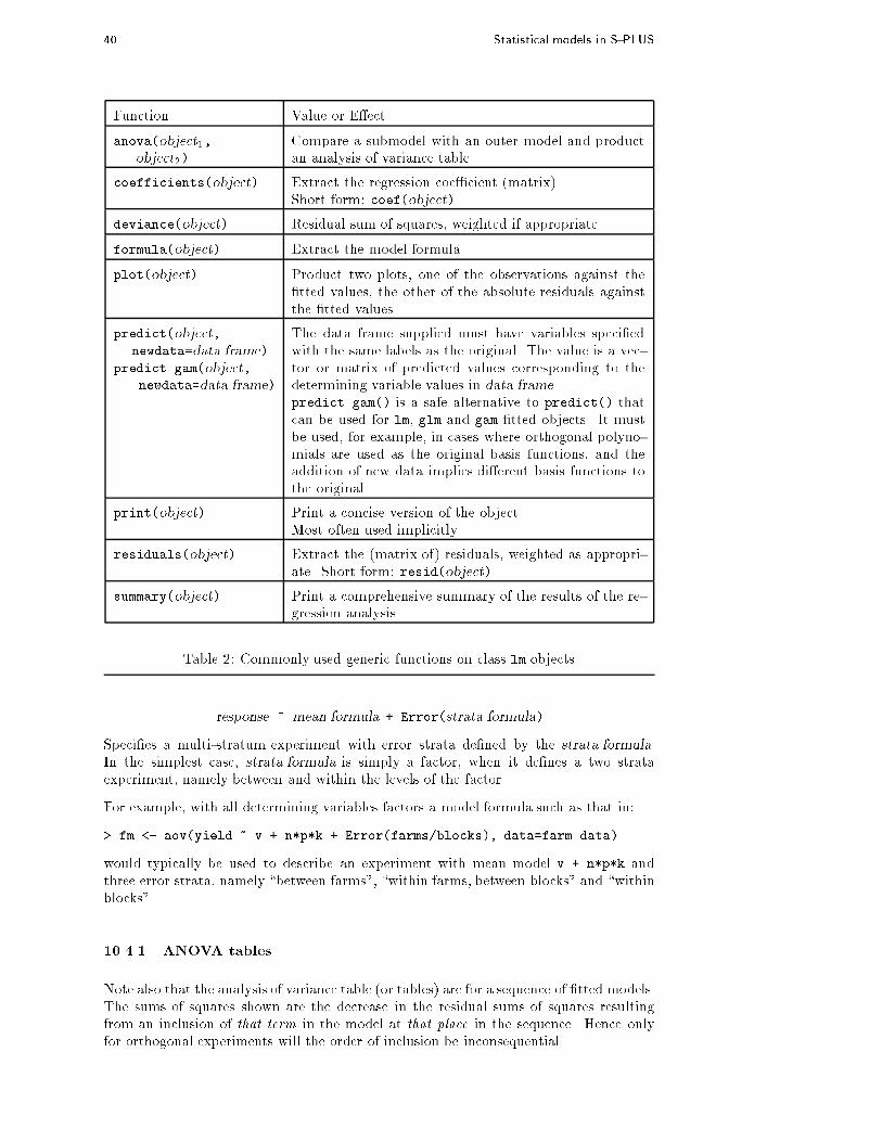
40 Statistical models in S-PLUS
Function Value or E�ect
anova(object1,
object2)
Compare a submodel with an outer model and productan analysis of variance table.
coefficients(object) Extract the regression coe�cient (matrix).Short form: coef(object).
deviance(object) Residual sum of squares, weighted if appropriate.
formula(object) Extract the model formula.
plot(object) Product two plots, one of the observations against the�tted values, the other of the absolute residuals againstthe �tted values.
predict(object,
newdata=data.frame)
predict.gam(object,
newdata=data.frame)
The data frame supplied must have variables speci�edwith the same labels as the original. The value is a vec-tor or matrix of predicted values corresponding to thedetermining variable values in data.frame.predict.gam() is a safe alternative to predict() thatcan be used for lm, glm and gam �tted objects. It mustbe used, for example, in cases where orthogonal polyno-mials are used as the original basis functions, and theaddition of new data implies di�erent basis functions tothe original.
print(object) Print a concise version of the object.Most often used implicitly.
residuals(object) Extract the (matrix of) residuals, weighted as appropri-ate. Short form: resid(object).
summary(object) Print a comprehensive summary of the results of the re-gression analysis.
Table 2: Commonly used generic functions on class lm objects
response ~ mean.formula + Error(strata.formula)
Speci�es a multi-stratum experiment with error strata de�ned by the strata.formula.In the simplest case, strata.formula is simply a factor, when it de�nes a two strataexperiment, namely between and within the levels of the factor.
For example, with all determining variables factors a model formula such as that in:
> fm <- aov(yield ~ v + n*p*k + Error(farms/blocks), data=farm.data)
would typically be used to describe an experiment with mean model v + n*p*k andthree error strata, namely \between farms", \within farms, between blocks" and \withinblocks".
10.4.1 ANOVA tables
Note also that the analysis of variance table (or tables) are for a sequence of �tted models.The sums of squares shown are the decrease in the residual sums of squares resultingfrom an inclusion of that term in the model at that place in the sequence. Hence onlyfor orthogonal experiments will the order of inclusion be inconsequential.

10.5 Updating �tted models. The ditto name \." 41
For multistratum experiments the procedure is �rst to project the response onto theerror strata, again in sequence, and to �t the mean model to each projection. Forfurther details, see Chambers and Hastie, x5.
A more exible alternative to the default full ANOVA table is to compare two or moremodels directly using the anova() function.
> anova(�tted.model.1, �tted.model.2, : : :)
The display is then an ANOVA table showing the di�erences between the �tted modelswhen �tted in sequence. The �tted models being compared would usually be an hierar-chical sequence, of course. This does not give di�erent information to the default, butrather makes it easier to comprehend and control.
10.5 Updating �tted models. The ditto name \."
The update() function is largely a convenience function that allows a model to be �ttedthat di�ers from one previously �tted usually by just a few additional or removed terms.Its form is
> new.model <- update(old.model, new.formula)
In the new.formula the special name consisting of a period, \.", only, can be used tostand for \the corresponding part of the old model formula". For example
> fm05 <- lm(y ~ x1 + x2 + x3 + x4 + x5, data=production)
> fm6 <- update(fm05, . ~ . + x6)
> smf6 <- update(fm6, sqrt(.) ~ .)
would �t a �ve variate multiple regression with variables (presumably) from the dataframe production, �t an additional model including a sixth regressor variable, and �t avariant on the model where the response had a square root transform applied.
Note especially that if the data= argument is speci�ed on the original call to the model �t-ting function, this information is passed on through the �tted model object to update()
and its allies.
The name \." can also be used in other contexts, but with slightly di�erent meaning.For example
> fmfull <- lm(y ~ . , data=production)
would �t a model with response y and regressor variables all other variables in the data
frame production.
Other functions for exploring incremental sequences of models are add1(), drop1(),step() and stepwise(). The names of these give a good clue to their purpose, but forfull details see the help document.
10.6 Generalized linear models; families
Generalized linear modelling is a development of linear models to accommodate both non-normal response distributions and transformations to linearity in a clean and straight-forward way. A generalized linear model may be described in terms of the followingsequence of assumptions:
� There is a response, y, of interest and stimulus variables x1, x2, : : :whose valuesin uence the distribution of the response.

42 Statistical models in S-PLUS
� The stimulus variables in uence the distribution of y through a single linear func-
tion, only. This linear function is called the linear predictor, and is usually written
� = �1x1 + �2x2 + � � �+ �pxp
hence xi has no in uence on the distribution of y if and only if �i = 0.
� The distribution of y is of the form
fY (y;�; ') = exp
�A
'fy�(�) � (�(�))g+ � (y; ')
�
where ' is a scale parameter, (possibly known), and is constant for all observa-tions, A represents a prior weight, assumed known but possibly varying with theobservations, and � is the mean of y. So it is assumed that the distribution of y isdetermined by its mean and possibly a scale parameter as well.
� The mean, �, is a smooth invertible function of the linear predictor:
� = m(�); � = m�1(�) = `(�)
and this inverse function, `(:) is called the link function.
These assumptions are loose enough to encompass a wide class of models useful in sta-tistical practice, but tight enough to allow the development of a uni�ed methodology ofestimation and inference, at least approximately. The reader is referred to any of thecurrent reference works on the subject for full details, such as
Generalized linear models by Peter McCullagh and John A Nelder, 2nd edition,Chapman and Hall, 1989, or
An introduction to generalized linear models by Annette J Dobson, Chapman andHall, 1990.
10.6.1 Families
The class of generalized linear models handled by facilities supplied in S-PLUS includesgaussian, binomial, poisson, inverse gaussian and gamma response distributions and alsoquasi-likelihoodmodels where the response distribution is not explicitly speci�ed. In thelatter case the variance function must be speci�ed as a function of the mean, but inother cases this function is implied by the response distribution.
Each response distribution admits a variety of link functions to connect the mean withthe linear predictor. Those automatically available are as in Table 3.
The combination of a response distribution, a link function and various other pieces ofinformation that are needed to carry out the modelling exercise is called the family ofthe generalized linear model.
10.6.2 The glm() function
Since the distribution of the response depends on the stimulus variables through a singlelinear function only, the same mechanism as was used for linear models can still be usedto specify the linear part of a generalized model. The family has to be speci�ed in adi�erent way.
The S-PLUS function to �t a generalized linear model is glm() which uses the form
> �tted.model <- glm(formula, family =family.generator, data=data.frame)
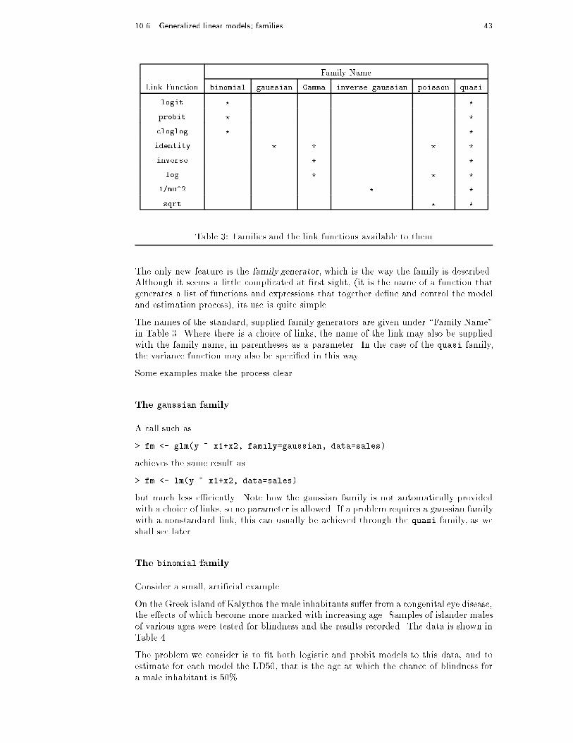
10.6 Generalized linear models; families 43
Family Name
Link Function binomial gaussian Gamma inverse.gaussian poisson quasi
logit ? ?
probit ? ?
cloglog ? ?
identity ? ? ? ?
inverse ? ?
log ? ? ?
1/mu^2 ? ?
sqrt ? ?
Table 3: Families and the link functions available to them
The only new feature is the family.generator, which is the way the family is described.Although it seems a little complicated at �rst sight, (it is the name of a function thatgenerates a list of functions and expressions that together de�ne and control the modeland estimation process), its use is quite simple.
The names of the standard, supplied family generators are given under \Family Name"in Table 3. Where there is a choice of links, the name of the link may also be suppliedwith the family name, in parentheses as a parameter. In the case of the quasi family,the variance function may also be speci�ed in this way.
Some examples make the process clear.
The gaussian family
A call such as
> fm <- glm(y ~ x1+x2, family=gaussian, data=sales)
achieves the same result as
> fm <- lm(y ~ x1+x2, data=sales)
but much less e�ciently. Note how the gaussian family is not automatically providedwith a choice of links, so no parameter is allowed. If a problem requires a gaussian familywith a nonstandard link, this can usually be achieved through the quasi family, as weshall see later.
The binomial family
Consider a small, arti�cial example.
On the Greek island of Kalythos the male inhabitants su�er from a congenital eye disease,the e�ects of which become more marked with increasing age. Samples of islander malesof various ages were tested for blindness and the results recorded. The data is shown inTable 4.
The problem we consider is to �t both logistic and probit models to this data, and toestimate for each model the LD50, that is the age at which the chance of blindness fora male inhabitant is 50%.

44 Statistical models in S-PLUS
Age: 20 35 45 55 70
No. tested: 50 50 50 50 50
No. blind: 6 17 26 37 44
Table 4: The Kalythos blindness data
If y is the number of blind at age x and n the number tested, both models have the form
y � B(n; F (�0 + �1x))
where for the probit case, F (z) = �(z) is the standard normal distribution function, andin the logit case, (the default), F (z) = ez=(1 + ez). In both cases the LD50 is
LD50 = ��0=�1
that is, the point at which the argument of the distribution function is zero.
The �rst step is to set the data up as a data frame
> kalythos <- data.frame(x=c(20,35,45,55,70), n=rep(50,5),
y=c(6,17,26,37,44))
To �t a binomial model using glm() there are two possibilities for the response:
� If the response is a vector it is assumed to hold binary data, and so must be a 0; 1vector.
� If the response is a two column matrix it is assumed that the �rst column holdsthe number of successes for the trial and the second holds the number of failures.
Here we need the second of these conventions, so we add a matrix to our data frame:
> kalythos$Ymat <- cbind(kalythos$y, kalythos$n - kalythos$y)
To �t the models we use
> fmp <- glm( Ymat~x, family=binomial(link=probit), data=kalythos)
> fml <- glm( Ymat~x, family=binomial, data=kalythos)
Since the logit link is the default the parameter may be omitted on the second call. Tosee the results of each �t we could use
> summary(fmp)
> summary(fml)
Both models �t (all too) well. To �nd the LD50 estimate we can use a simple function:
> ld50 <- function(b) -b[1]/b[2]
> ldp <- ld50(coef(fmp)); ldl <- ld50(coef(fmp)); c(ldp, ldl)
The actual estimates from this data are 43.663 years and 43.601 years respectively.
Poisson models
With the poisson family the default link is the log, and in practice the major use ofthis family is to �t surrogate poisson log-linear models to frequency data, whose actualdistribution is often multinomial. This is a large and important subject we will not
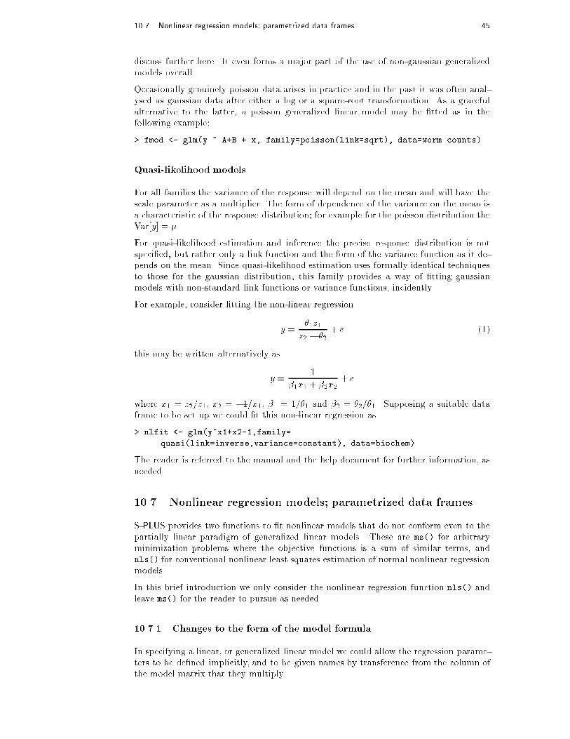
10.7 Nonlinear regression models; parametrized data frames 45
discuss further here. It even forms a major part of the use of non-gaussian generalizedmodels overall.
Occasionally genuinely poisson data arises in practice and in the past it was often anal-ysed as gaussian data after either a log or a square-root transformation. As a gracefulalternative to the latter, a poisson generalized linear model may be �tted as in thefollowing example:
> fmod <- glm(y ~ A+B + x, family=poisson(link=sqrt), data=worm.counts)
Quasi-likelihood models
For all families the variance of the response will depend on the mean and will have thescale parameter as a multiplier. The form of dependence of the variance on the mean isa characteristic of the response distribution; for example for the poisson distribution theVar[y] = �.
For quasi-likelihood estimation and inference the precise response distribution is notspeci�ed, but rather only a link function and the form of the variance function as it de-pends on the mean. Since quasi-likelihood estimation uses formally identical techniquesto those for the gaussian distribution, this family provides a way of �tting gaussianmodels with non-standard link functions or variance functions, incidently.
For example, consider �tting the non-linear regression
y =�1z1
z2 � �2+ e (1)
this may be written alternatively as
y =1
�1x1 + �2x2+ e
where x1 = z2=z1, x2 = �1=x1, �1 = 1=�1 and �2 = �2=�1. Supposing a suitable dataframe to be set up we could �t this non-linear regression as
> nlfit <- glm(y~x1+x2-1,family=
quasi(link=inverse,variance=constant), data=biochem)
The reader is referred to the manual and the help document for further information, asneeded.
10.7 Nonlinear regression models; parametrized data frames
S-PLUS provides two functions to �t nonlinear models that do not conform even to thepartially linear paradigm of generalized linear models. These are ms() for arbitraryminimization problems where the objective functions is a sum of similar terms, andnls() for conventional nonlinear least squares estimation of normal nonlinear regressionmodels.
In this brief introduction we only consider the nonlinear regression function nls() andleave ms() for the reader to pursue as needed.
10.7.1 Changes to the form of the model formula
In specifying a linear, or generalized linear model we could allow the regression parame-ters to be de�ned implicitly, and to be given names by transference from the column ofthe model matrix that they multiply.
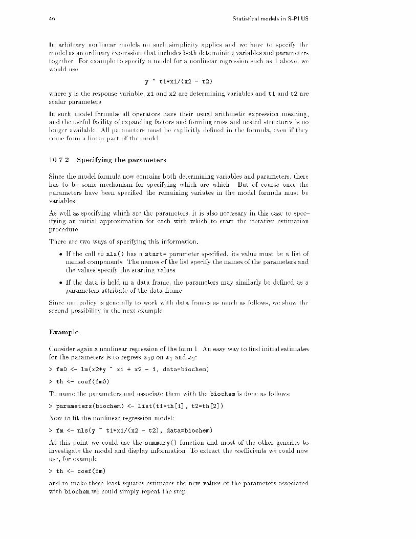
46 Statistical models in S-PLUS
In arbitrary nonlinear models no such simplicity applies and we have to specify themodel as an ordinary expression that includes both determining variables and parameterstogether. For example to specify a model for a nonlinear regression such as 1 above, wewould use
y ~ t1*x1/(x2 - t2)
where y is the response variable, x1 and x2 are determining variables and t1 and t2 arescalar parameters.
In such model formul� all operators have their usual arithmetic expression meaning,and the useful facility of expanding factors and forming cross and nested structures is nolonger available. All parameters must be explicitly de�ned in the formula, even if theycome from a linear part of the model.
10.7.2 Specifying the parameters
Since the model formula now contains both determining variables and parameters, therehas to be some mechanism for specifying which are which. But of course once theparameters have been speci�ed the remaining variates in the model formula must bevariables.
As well as specifying which are the parameters, it is also necessary in this case to spec-ifying an initial approximation for each with which to start the iterative estimationprocedure.
There are two ways of specifying this information:
� If the call to nls() has a start= parameter speci�ed, its value must be a list ofnamed components. The names of the list specify the names of the parameters andthe values specify the starting values.
� If the data is held in a data frame, the parameters may similarly be de�ned as aparameters attribute of the data frame.
Since our policy is generally to work with data frames as much as follows, we show thesecond possibility in the next example.
Example
Consider again a nonlinear regression of the form 1. An easy way to �nd initial estimatesfor the parameters is to regress x2y on x1 and x2:
> fm0 <- lm(x2*y ~ x1 + x2 - 1, data=biochem)
> th <- coef(fm0)
To name the parameters and associate them with the biochem is done as follows:
> parameters(biochem) <- list(t1=th[1], t2=th[2])
Now to �t the nonlinear regression model:
> fm <- nls(y ~ t1*x1/(x2 - t2), data=biochem)
At this point we could use the summary() function and most of the other generics toinvestigate the model and display information. To extract the coe�cients we could nowuse, for example
> th <- coef(fm)
and to make these least squares estimates the new values of the parameters associatedwith biochem we could simply repeat the step

10.8 Some non-standard models 47
> parameters(biochem) <- list(t1=th[1], t2=th[2])
Note that the function parameters()may either be used as an expression, in which caseit extracts the list of parameters from a data frame, or it may be used as the target foran assignment, in which case it accepts a parameter list for a speci�ed data frame. Inthis respect it is very similar to the attributes() function. There is also a functionparam() analogous to attr(), which handles one parameter at a time under a characterstring name.
10.8 Some non-standard models
We conclude this section with just a brief mention of some of the other facilities availablein S-PLUS for special regression and data analysis problems.
Local approximating regressions. The loess() function �ts a nonparametric re-gression by using a locally weighted regression. Such regressions are useful forhighlighting a trend in messy data or for data reduction to give some insight intoa large data set.
Robust regression There are several functions available for �tting regression modelsin a way resistant to the in uence of extreme outliers in the data. The mostsophisticated of these is rreg(), but others include lmsfit() for least mediansquares regression and l1fit() for regression using the L1�norm. However thesedo not as yet have the facility of using formul� to specify the model function, forexample, and conform to an older protocol, which makes them sometimes rathertedious to use. There is also a robust() facility to change a glm family object intoa robust version for use with the glm() model �tting function.
Generalized additive models. This technique aims to construct an regression func-tion from smooth additive functions of the determining variables, usually one foreach determining variable. The function gam() is in many ways similar to the othermodel �tting functions outlined above. In addition there are other model �ttingfunctions that do a similar job. These include avas() and ace(). On the otherhand ppreg() is available for projection pursuit regression, but this technique isstill very much in need of a complete theoretical treatment and further practicalexperience. These latter functions are again conforming to an older protocol formodel �tting functions and lack the convenience of the newer functions.
Tree based models Rather than seek an explicit global linear model for prediction orinterpretation, tree based models seek to bifurcate the data, recursively, at criticalpoints of the determining variables in order to partition the data ultimately intogroups that are as homogeneous as possible within, and as heterogeneous as possiblebetween. The results often lead to insights that other data analysis methods tendnot to yield.
Models are again speci�ed in the ordinary linear model form. The model �ttingfunction is tree(), but many other generic functions such as plot() and text()
are well adapted to displaying the results of a tree-based model �t in a graphicalway.
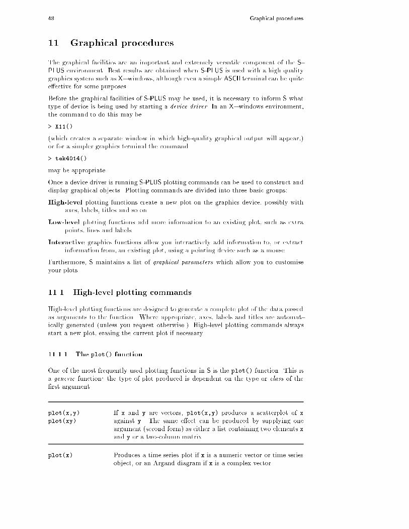
48 Graphical procedures
11 Graphical procedures
The graphical facilities are an important and extremely versatile component of the S-
PLUS environment. Best results are obtained when S-PLUS is used with a high qualitygraphics system such as X�windows, although even a simple ASCII terminal can be quitee�ective for some purposes.
Before the graphical facilities of S-PLUS may be used, it is necessary to inform S whattype of device is being used by starting a device driver. In an X�windows environment,the command to do this may be
> X11()
(which creates a separate window in which high-quality graphical output will appear,)or for a simpler graphics terminal the command
> tek4014()
may be appropriate.
Once a device driver is running S-PLUS plotting commands can be used to construct anddisplay graphical objects. Plotting commands are divided into three basic groups:
High-level plotting functions create a new plot on the graphics device, possibly withaxes, labels, titles and so on.
Low-level plotting functions add more information to an existing plot, such as extrapoints, lines and labels.
Interactive graphics functions allow you interactively add information to, or extractinformation from, an existing plot, using a pointing device such as a mouse.
Furthermore, S maintains a list of graphical parameters which allow you to customiseyour plots.
11.1 High-level plotting commands
High-level plotting functions are designed to generate a complete plot of the data passedas arguments to the function. Where appropriate, axes, labels and titles are automat-ically generated (unless you request otherwise.) High-level plotting commands alwaysstart a new plot, erasing the current plot if necessary.
11.1.1 The plot() function
One of the most frequently used plotting functions in S is the plot() function. This isa generic function: the type of plot produced is dependent on the type or class of the�rst argument.
plot(x,y)
plot(xy)
If x and y are vectors, plot(x,y) produces a scatterplot of xagainst y. The same e�ect can be produced by supplying oneargument (second form) as either a list containing two elements xand y or a two-column matrix.
plot(x) Produces a time series plot if x is a numeric vector or time seriesobject, or an Argand diagram if x is a complex vector.

11.1 High-level plotting commands 49
plot(f)
plot(f,y)
f is a factor object, y is a numeric vector. The �rst form generatesa bar plot of f; the second form produces boxplots of y for eachlevel of f.
plot(df)
plot(~ expr)
plot(y ~ expr)
df is a data frame, y is any object, expr is a list of object namesseparated by `+' (e.g. a + b + c). The �rst two forms producedistributional plots of the variables in a data frame (�rst form)or of a number of named objects (second form). The third formplots y against every object named in expr.
11.1.2 Displaying multivariate data
S provides two very useful functions for representing multivariate data. If X is a numericmatrix or data frame, the command
> pairs(X)
produces a pairwise scatterplot matrix of the variables de�ned by the columns of X, i.e.every column of X is plotted against every other column of X and the resulting n(n � 1)plots are arranged in a matrix with plot scales constant over the rows and columns ofthe matrix.
When three or four variables are involved a coplot may be more enlightening. If a and b
are numeric vectors and c is a numeric vector or factor object (all of the same length),then the command
> coplot(a ~ b | c)
produces a number of scatterplots of a against b for given values of c. If c is a factor,this simply means that a is plotted against b for every level of c. When c is numeric,it is divided into a number of conditioning intervals and for each interval a is plottedagainst b for values of c within the interval. The number and position of intervals can becontrolled with given.values= argument to coplot()| the function co.intervals()
is useful for selecting intervals. You can also use two \given" variables with a commandlike
> coplot(a ~ b | c + d)
which produces scatterplots of a against b for every joint conditioning interval of c andd.
The coplot() and pairs() function both take an argument panel= which can be usedto customise the type of plot which appears in each panel. The default is points() toproduce a scatterplot but by supplying some other low-level graphics function of twovectors x and y as the value of panel= you can produce any type of plot you wish. Anexample panel function useful for coplots is panel.smooth().
11.1.3 Display graphics
Other high-level graphics functions produce di�erent types of plots. Some examples are:
tsplot(x1,x2,...) Plots any number of time series on the same scale. This auto-matic simultaneous scaling feature is also useful when the xi's areordinary numeric vectors, in which case they are plotted againstthe numbers 1; 2; 3; : : :.

50 Graphical procedures
qqnorm(x)
qqplot(x,y)
Distribution-comparison plots. The �rst form plots the numericvector x against the expected Normal order scores (a normal scoresplot.) The second form plots the quantiles of x against those of yto compare their respective distributions.
hist(x)
hist(x,nclass=n)
hist(x,breaks=: : :)
Produces a histogram of the numeric vector x. A sensible numberof classes is usually chosen, but a recommendation can be givenwith the nclass= argument. Alternatively, the breakpoints canbe speci�ed exactly with the breaks= argument. If the probabil-ity=T argument is given, the bars represent relative frequenciesinstead of counts.
dotchart(x,: : :) Construct a dotchart of the data in x. In a dotchart the y�axisgives a labelling of the data in x and the x�axis gives its value.For example it allows easy visual selection of all data entries withvalues lying in speci�ed ranges.
pie(slices,
names,
explode=: : :)
Make a pie diagram, including the possibility of some pieces dis-placed or \exploded" out from the centre. (Pie diagrams are es-pecially good for showing to administrators and bosses, but notmuch else, in my opinion.)
11.1.4 Arguments to high-level plotting functions
There are a number of arguments which may be passed to high-level graphics functions,as follows:
add=T Forces the function to act as a low-level graphics function, super-imposing the plot on the current plot (some functions only).
axes=F Suppresses generation of axes | useful for adding your own cus-tom axes with the axis() function. The default, axes=T, meansinclude axes.
log="x"
log="y"
log="xy"
Causes the x, y or both axes to be logarithmic. Only works forscatterplots (and variants).
type= The type= argument controls the type of plot produced, as follows:
type="p" Plot individual points (the default)
type="l" Plot lines
type="b" Plot points connected by lines (\both")
type="o" Plot points overlaid by lines
type="h" Plot vertical lines from points to the zero axis (\high-density")
type="s"
type="S"
Step-function plots. In the �rst form, the top of the vertical de�nesthe point; in the second, the bottom.
type="n" No plotting at all. However axes are still drawn (by default) andthe coordinate system is set up according to the data. Ideal forcreating plots with subsequent low-level graphics functions.

11.2 Low-level plotting commands 51
xlab="string"
ylab="string"
Axis labels for the x and y axes. Use these arguments to changethe default labels, usually the names of the objects used in thecall to the high-level plotting function.
main="string" Figure title, placed at the top of the plot in a large font.
sub="string" Sub-title, placed just below the x-axis in a smaller font.
11.2 Low-level plotting commands
Sometimes the high-level plotting functions don't produce exactly the kind of plot youdesire. In this case, low-level plotting commands can be used to add extra information(such as points, lines or text) to the current plot.
Some of the more useful low-level plotting functions are:
points(x,y)
lines(x,y)
Adds points or connected lines to the current plot. plot()'s type=argument can also be passed to these functions (and defaults to"p" for points() and "l" for lines().)
text(x, y,
labels, : : :)
Add text to a plot at points given by x, y. Normally labels isan integer or character vector in which case labels[i] is plottedat point (x[i], y[i]). The default is 1:length(x).
Note: This function is often used in the sequence> plot(x, y, type="n"); text(x, y, names)
The graphics parameter type="n" suppresses the points but setsup the axes, and the text() function supplies special characters,as speci�ed by the character vector names for the points.
abline(a, b)
abline(h=y)
abline(v=x)
abline(lm.obj)
Adds a line of slope b and intercept a to the current plot. h=y
may be used to specify y-coordinates for the heights of horizontallines to go across a plot, and v=x similarly for the x-coordinatesfor vertical lines. Also lm.obj may be list with a $coefficients
component of length 2 (such as the result of model-�tting func-
tions,) which are taken as an intercept and slope, in that order.
polygon(x, y,
: : :)
Draws a polygon de�ned by the ordered vertices in (x,y). and(optionally) shade it in with hatch lines, or �ll it if the graphicsdevice allows the �lling of �gures.
legend(x,y,
legend,...)
Adds a legend to the current plot at the speci�ed position. Plot-ting characters, line styles, colours etc. are identi�ed with the la-bels in the character vector legend. At least one other argumentv (a vector the same length as legend) with the correspondingvalues of the plotting unit must also be given, as follows:
legend( ,angle=v) Shading angles
legend( ,
density=v)
Shading densities
legend( ,fill=v) Colours for �lled boxes
legend( ,col=v) Colours in which points or lines will be drawn

52 Graphical procedures
legend( ,lty=v) Line styles
legend( ,pch=v) Plotting characters (character vector)
legend( ,marks=v) Plotting symbols, as obtained when using a numeric argument topch= (numeric vector).
title(main,sub) Adds a title main to the top of the current plot in a large font and(optionally) a sub-title sub at the bottom in a smaller font.
axis(side,...) Adds an axis to the current plot on the side given by the �rstargument (1 to 4, counting clockwise from the bottom.) Otherarguments control the positioning of the axis within or beside theplot, and tick positions and labels. Useful for adding custom axesafter calling plot() with the axes=F argument.
Low-level plotting functions usually require some positioning information (e.g. x and y
coordinates) to determine where to place the new plot elements. Coordinates are given interms of user coordinates which are de�ned by the previous high-level graphics commandand are chosen based on the supplied data.
Where x and y arguments are required, it is also su�cient to supply a single argumentbeing a list with elements named x and y. Similarly a matrix with two columns is alsovalid input. In this way functions such as locator() (see below) may be used to specifypositions on a plot interactively.
11.3 Interactive graphics functions
S also provides functions which allow users to extract or add information to a plot usinga mouse. The simplest of these is the locator() function:
locator(n,type) Waits for the user to select locations on the current plot using theleft mouse button. This continues until n (default 500) points havebeen selected, or the middle mouse button is pressed. The type
argument allows for plotting at the selected points and has thesame e�ect as for high-level graphics commands; the default is no
plotting. locator() returns the locations of the points selectedas a list with two components x and y.
locator() is usually called with no arguments. It is particularly useful for interactivelyselecting positions for graphic elements such as legends or labels when it is di�cult tocalculate in advance where the graphic should be placed. For example, to place someinformative text near an outlying point, the command
> text(locator(1), "Outlier", adj=0)
may be useful. locator() will still work if the current device does not support a mouse;in this case the user will be prompted for x and y coordinates.
identify(x,y,
labels)
Allow the user to highlight any of the points de�ned by x andy (using the left mouse button) by plotting the correspondingcomponent of labels nearby (or the index number of the pointif labels is absent). Returns the indices of the selected pointswhen the middle button is pressed.
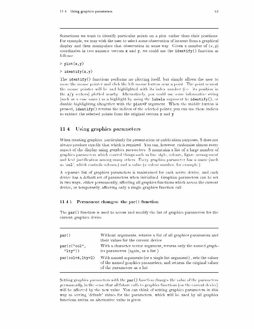
11.4 Using graphics parameters 53
Sometimes we want to identify particular points on a plot, rather than their positions.For example, we may wish the user to select some observation of interest from a graphicaldisplay and then manipulate that observation in some way. Given a number of (x; y)coordinates in two numeric vectors x and y, we could use the identify() function asfollows:
> plot(x,y)
> identify(x,y)
The identify() functions performs no plotting itself, but simply allows the user tomove the mouse pointer and click the left mouse button near a point. The point nearestthe mouse pointer will be and highlighted with its index number (i.e. its position inthe x/y vectors) plotted nearby. Alternatively, you could use some informative string(such as a case name) as a highlight by using the labels argument to identify(), ordisable highlighting altogether with the plot=F argument. When the middle button ispressed, identify() returns the indices of the selected points; you can use these indicesto extract the selected points from the original vectors x and y.
11.4 Using graphics parameters
When creating graphics, particularly for presentation or publication purposes, S does notalways produce exactly that which is required. You can, however, customise almost everyaspect of the display using graphics parameters. S maintains a list of a large number ofgraphics parameters which control things such as line style, colours, �gure arrangementand text justi�cation among many others. Every graphics parameter has a name (suchas `col', which controls colours,) and a value (a colour number, for example.)
A separate list of graphics parameters is maintained for each active device, and eachdevice has a default set of parameters when initialised. Graphics parameters can be setin two ways: either permanently, a�ecting all graphics functions which access the currentdevice; or temporarily, a�ecting only a single graphics function call.
11.4.1 Permanent changes: the par() function
The par() function is used to access and modify the list of graphics parameters for thecurrent graphics device.
par() Without arguments, returns a list of all graphics parameters andtheir values for the current device.
par(c("col",
"lty"))
With a character vector argument, returns only the named graph-ics parameters (again, as a list.)
par(col=4,lty=2) With named arguments (or a single list argument) , sets the valuesof the named graphics parameters, and returns the original valuesof the parameters as a list.
Setting graphics parameters with the par() function changes the value of the parameterspermanently, in the sense that all future calls to graphics functions (on the current device)will be a�ected by the new value. You can think of setting graphics parameters in thisway as setting `default' values for the parameters, which will be used by all graphicsfunctions unless an alternative value is given.

54 Graphical procedures
Note that calls to par() always a�ect the global values of graphics parameters, evenwhen par() is called from within a function. This is often undesirable behaviour |usually we want to set some graphics parameters, do some plotting, and then restore theoriginal values so as not to a�ect the user's S session. You can restore the initial valuesby saving the result of par() when making changes, and restoring the initial values whenplotting is complete.
> oldpar <- par(col=4,lty=2)
: : :plotting commands : : :
> par(oldpar)
11.4.2 Temporary changes: arguments to graphics functions
Graphics parameters may also be passed to (almost) any graphics function as namedarguments. This has the same e�ect as passing the arguments to the par() function,except that the changes only last for the duration of the function call. For example:
> plot(x,y,pch="+")
produces a scatterplot using a plus sign as the plotting character, without changing thedefault plotting character for future plots.
11.5 Graphics parameters list
The following sections detail many of the commonly-used graphical parameters. The Shelp documentation for the par() function provides a more concise summary; this isprovided as a somewhat more detailed alternative.
Graphics parameters will be presented in the following form:
name=value A description of the parameter's e�ect. name is the name of the pa-rameter, i.e. the argument name to use in calls to par() or a graphicsfunction. value is a typical value you might use when setting theparameter.
11.5.1 Graphical elements
S plots are made up of points, lines, text and polygons (�lled regions.) Graphical pa-rameters exist which control how these graphical elements are drawn, as follows:
pch="+" Character to be used for plotting points. The default varies withgraphics drivers, but it is usually `*' for terminals or window devices,and `�' for PostScript devices. Plotted points tend to appear slightlyabove or below the appropriate position unless you use "." as theplotting character, which produces centred points.
pch=4 When pch is given as an integer between 0 and 18 inclusive, a spe-cialised plotting symbol is produced. To see what the symbols are,use the command
> legend(locator(1),as.character(0:18),marks=0:18)
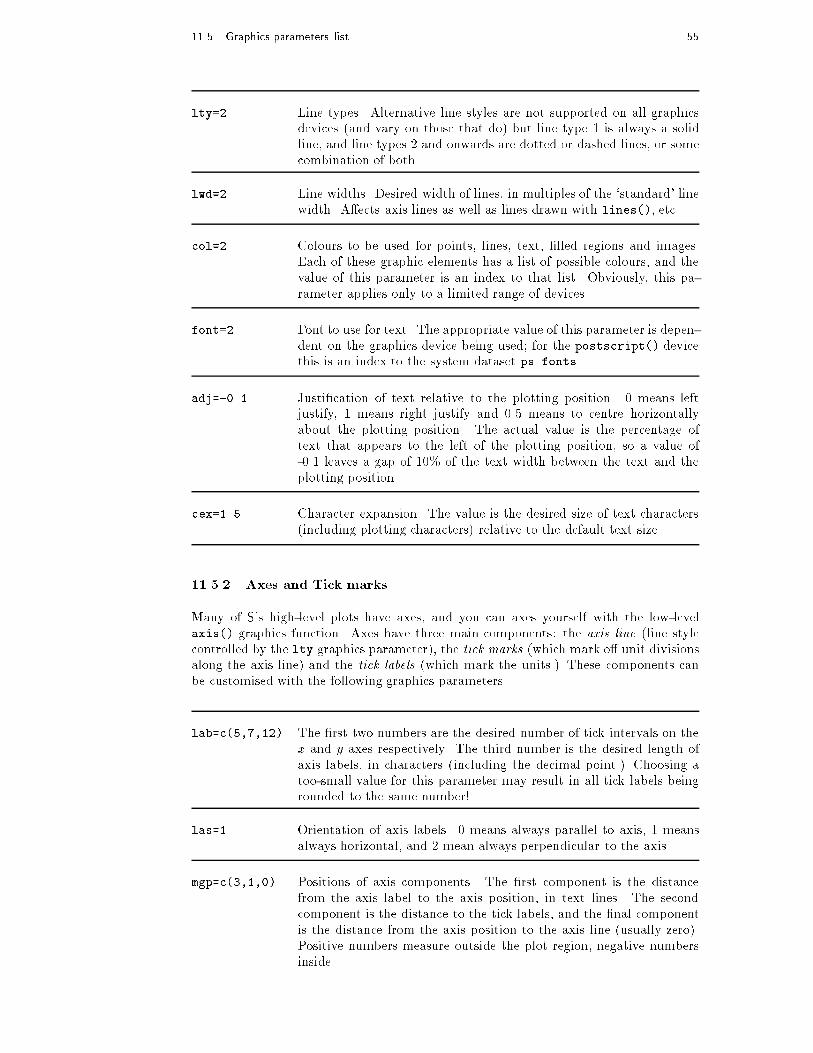
11.5 Graphics parameters list 55
lty=2 Line types. Alternative line styles are not supported on all graphicsdevices (and vary on those that do) but line type 1 is always a solidline, and line types 2 and onwards are dotted or dashed lines, or somecombination of both.
lwd=2 Line widths. Desired width of lines, in multiples of the `standard' linewidth. A�ects axis lines as well as lines drawn with lines(), etc.
col=2 Colours to be used for points, lines, text, �lled regions and images.Each of these graphic elements has a list of possible colours, and thevalue of this parameter is an index to that list. Obviously, this pa-rameter applies only to a limited range of devices.
font=2 Font to use for text. The appropriate value of this parameter is depen-dent on the graphics device being used; for the postscript() devicethis is an index to the system dataset ps.fonts.
adj=-0.1 Justi�cation of text relative to the plotting position. 0 means leftjustify, 1 means right justify and 0.5 means to centre horizontallyabout the plotting position. The actual value is the percentage oftext that appears to the left of the plotting position, so a value of-0.1 leaves a gap of 10% of the text width between the text and theplotting position.
cex=1.5 Character expansion. The value is the desired size of text characters(including plotting characters) relative to the default text size.
11.5.2 Axes and Tick marks
Many of S's high-level plots have axes, and you can axes yourself with the low-levelaxis() graphics function. Axes have three main components: the axis line (line stylecontrolled by the lty graphics parameter), the tick marks (which mark o� unit divisionsalong the axis line) and the tick labels (which mark the units.) These components canbe customised with the following graphics parameters.
lab=c(5,7,12) The �rst two numbers are the desired number of tick intervals on thex and y axes respectively. The third number is the desired length ofaxis labels, in characters (including the decimal point.) Choosing atoo-small value for this parameter may result in all tick labels beingrounded to the same number!
las=1 Orientation of axis labels. 0 means always parallel to axis, 1 meansalways horizontal, and 2 mean always perpendicular to the axis.
mgp=c(3,1,0) Positions of axis components. The �rst component is the distancefrom the axis label to the axis position, in text lines. The secondcomponent is the distance to the tick labels, and the �nal componentis the distance from the axis position to the axis line (usually zero).Positive numbers measure outside the plot region, negative numbersinside.
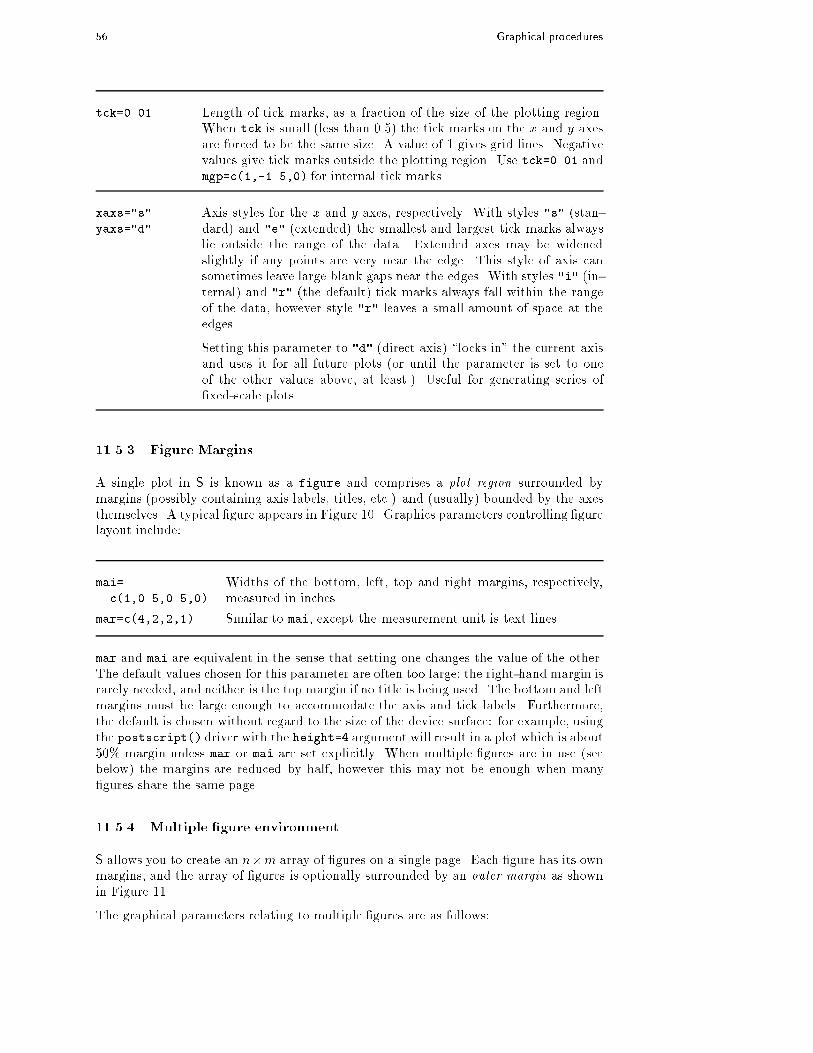
56 Graphical procedures
tck=0.01 Length of tick marks, as a fraction of the size of the plotting region.When tck is small (less than 0.5) the tick marks on the x and y axesare forced to be the same size. A value of 1 gives grid lines. Negativevalues give tick marks outside the plotting region. Use tck=0.01 andmgp=c(1,-1.5,0) for internal tick marks.
xaxs="s"
yaxs="d"
Axis styles for the x and y axes, respectively. With styles "s" (stan-dard) and "e" (extended) the smallest and largest tick marks alwayslie outside the range of the data. Extended axes may be widenedslightly if any points are very near the edge. This style of axis cansometimes leave large blank gaps near the edges. With styles "i" (in-ternal) and "r" (the default) tick marks always fall within the rangeof the data, however style "r" leaves a small amount of space at theedges.
Setting this parameter to "d" (direct axis) \locks in" the current axisand uses it for all future plots (or until the parameter is set to oneof the other values above, at least.) Useful for generating series of�xed-scale plots.
11.5.3 Figure Margins
A single plot in S is known as a figure and comprises a plot region surrounded bymargins (possibly containing axis labels, titles, etc.) and (usually) bounded by the axesthemselves. A typical �gure appears in Figure 10. Graphics parameters controlling �gurelayout include:
mai=
c(1,0.5,0.5,0)
Widths of the bottom, left, top and right margins, respectively,measured in inches.
mar=c(4,2,2,1) Similar to mai, except the measurement unit is text lines.
mar and mai are equivalent in the sense that setting one changes the value of the other.The default values chosen for this parameter are often too large; the right-hand margin israrely needed, and neither is the top margin if no title is being used. The bottom and leftmargins must be large enough to accommodate the axis and tick labels. Furthermore,the default is chosen without regard to the size of the device surface: for example, usingthe postscript() driver with the height=4 argument will result in a plot which is about50% margin unless mar or mai are set explicitly. When multiple �gures are in use (seebelow) the margins are reduced by half, however this may not be enough when many�gures share the same page.
11.5.4 Multiple �gure environment
S allows you to create an n�m array of �gures on a single page. Each �gure has its ownmargins, and the array of �gures is optionally surrounded by an outer margin as shownin Figure 11.
The graphical parameters relating to multiple �gures are as follows:

11.5 Graphics parameters list 57
6
?
6
� - -
. . . . . . . . . . . . . . . . . . . . . . . . . . . .............................
mai[2]
mar[3]
**
*
*
*
*
*
*
*
*
*
*
*
y
mai[1]x
Plot region
Margin
Figure 10: Anatomy of an S �gure
mfcol=c(3,2)
mfrow=c(2,4)
Set size of multiple �gure array. The �rst value is the number ofrows; the second is the number of columns. The only di�erencebetween these two parameters is that setting mfcol causes �guresto be �lled by column; mfrow �lls by rows. The arrangement inFigure 11 would have been created by setting mfrow=c(3,2); the�gure shows the page after four plots have been drawn.
mfg=c(2,2,3,2) Position of current �gure in a multiple �gure environment. The�rst two numbers are the row and column of the current �gure; thelast two are the number of rows and columns in the multiple �gurearray. Set this parameter to jump between �gures in the array.You can even use di�erent values for the last two numbers thanthe \true" values for unequally-sized �gures on the same page.
fig=c(4,9,1,4)/10 Position of the current �gure on the page. Values are the po-sitions of the left, right, bottom and top edges respectively, asa percentage of the page measured from the bottom left corner.The example value would be for a �gure in the bottom right ofthe page. Set this parameter for arbitrary positioning of �gureswithin a page.
oma=c(2,0,3,0)
omi=c(0,0,0.8,0)
Size of outer margins. Like mar and mai, the �rst measures in textlines and the second in inches, starting with the bottom marginand working clockwise.

58 Graphical procedures
� -
6
?
�� � H H �
��
� � Q Q ��
**
***
****
*
**
* * **
**
**
**
*
omi[2]omi[3]
mfrow=c(3,2)
oma[1]
mfg=c(2,2,3,2)
Figure 11: Page layout in multiple �gure mode
Outer margins are particularly useful for page-wise titles, etc. Text can be added to theouter margins with the mtext() function with argument outer=T. There are no outermargins by default, however, so you must create them explicitly using oma or omi.
11.6 Device drivers
S can generate graphics (of varying levels of quality) on almost any type of display orprinting device. Before this can begin, however, S needs to be informed what type ofdevice it is dealing with. This is done by starting a device driver. The purpose of adevice driver is to convert graphical instructions from S (`draw a line,' for example) into
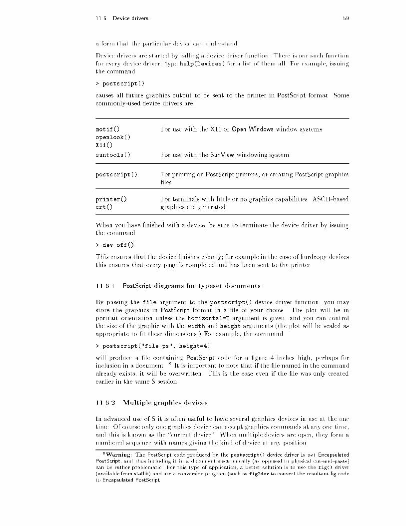
11.6 Device drivers 59
a form that the particular device can understand.
Device drivers are started by calling a device driver function. There is one such functionfor every device driver: type help(Devices) for a list of them all. For example, issuingthe command
> postscript()
causes all future graphics output to be sent to the printer in PostScript format. Somecommonly-used device drivers are:
motif()
openlook()
X11()
For use with the X11 or Open Windows window systems.
suntools() For use with the SunView windowing system.
postscript() For printing on PostScript printers, or creating PostScript graphics�les.
printer()
crt()
For terminals with little or no graphics capabilities. ASCII-basedgraphics are generated.
When you have �nished with a device, be sure to terminate the device driver by issuingthe command
> dev.off()
This ensures that the device �nishes cleanly; for example in the case of hardcopy devicesthis ensures that every page is completed and has been sent to the printer.
11.6.1 PostScript diagrams for typeset documents.
By passing the file argument to the postscript() device driver function, you maystore the graphics in PostScript format in a �le of your choice. The plot will be inportrait orientation unless the horizontal=T argument is given, and you can controlthe size of the graphic with the width and height arguments (the plot will be scaled asappropriate to �t these dimensions.) For example, the command
> postscript("file.ps", height=4)
will produce a �le containing PostScript code for a �gure 4 inches high, perhaps forinclusion in a document. 8 It is important to note that if the �le named in the commandalready exists, it will be overwritten. This is the case even if the �le was only createdearlier in the same S session.
11.6.2 Multiple graphics devices
In advanced use of S it is often useful to have several graphics devices in use at the onetime. Of course only one graphics device can accept graphics commands at any one time,and this is known as the \current device". When multiple devices are open, they form anumbered sequence with names giving the kind of device at any position.
8Warning: The PostScript code produced by the postscript() device driver is not Encapsulated
PostScript, and thus including it in a document electronically (as opposed to physical cut-and-paste)can be rather problematic. For this type of application, a better solution is to use the fig() driver(available from statlib) and use a conversion program (such as fig2dev to convert the resultant �g code
to Encapsulated PostScript.

60 Graphical procedures
The main commands used for operating with multiple devices, and their meanings areas follows:
motif()
postscript()
: : :
Each new call to a device driver function opens a new graphicsdevice, thus extending by one the device list. This device becomesthe current device, to which graphics output will be sent.
dev.list() returns the number and name of all active devices. The device atposition 1 on the list is always the \null device" which does notaccept graphics commands at all.
dev.next()
dev.prev()
returns the number and name of the graphics device next to, orprevious to the current device, respectively.
dev.set(which=k) can be used to change the current graphics device to the one atposition k of the device list. Returns the number and label of thedevice.
def.off(k) Terminate the graphics device at point k of the device list. Forsome devices, such as postscript devices, this will either print the�le immediately or correctly complete the �le for later printing,depending on how the device was initiated.
dev.copy(device,
: : :, which=k)
dev.print(device,
: : :, which=k)
Make a copy of the device k. device is a device function, suchas postscript, with extra arguments, if needed, speci�ed by : : : .dev.print is similar, but the copied device is immediately closed,so that end actions, such as printing hardcopies, are immediatelyperformed. (See also printgraph()).
graphics.off() Terminate all graphics devices on the list, except the null device.
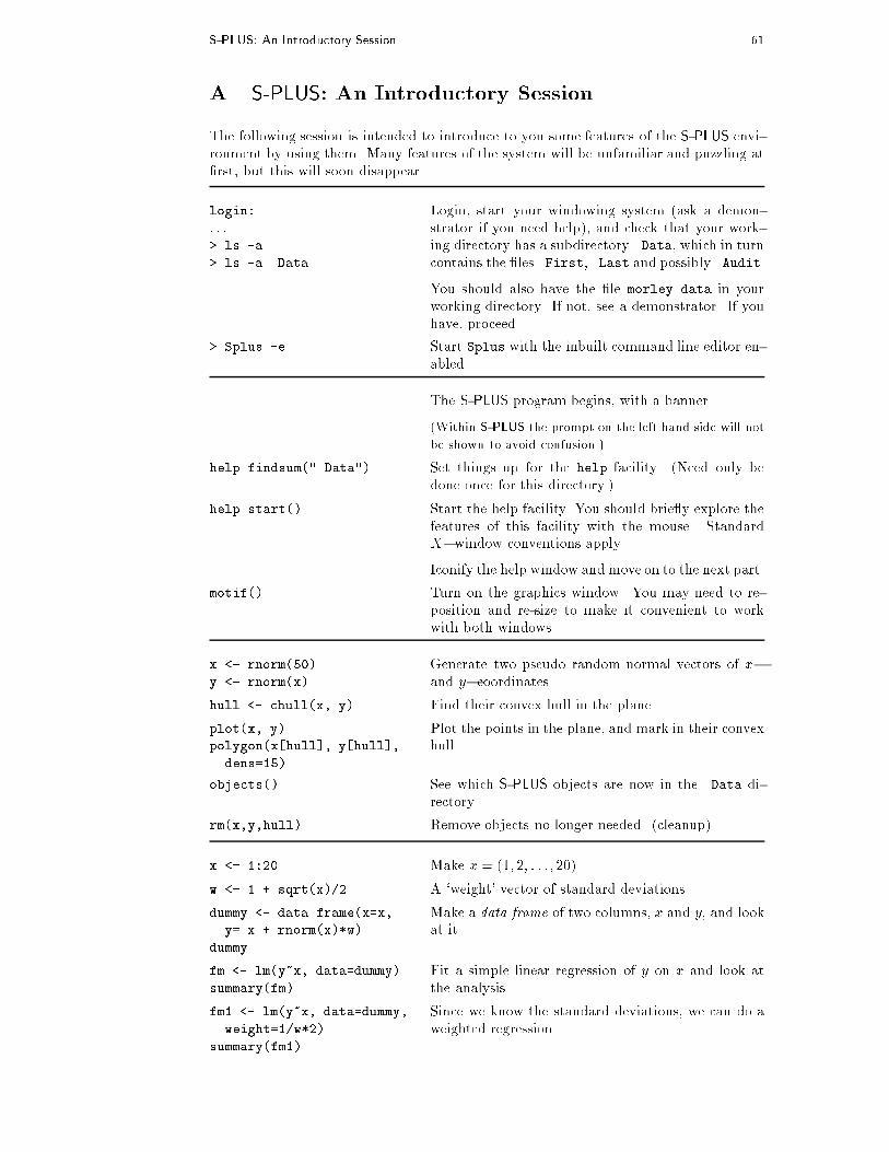
S-PLUS: An Introductory Session 61
A S-PLUS: An Introductory Session
The following session is intended to introduce to you some features of the S-PLUS envi-ronment by using them. Many features of the system will be unfamiliar and puzzling at�rst, but this will soon disappear.
login:
: : :
> ls -a
> ls -a .Data
Login, start your windowing system (ask a demon-strator if you need help), and check that your work-ing directory has a subdirectory .Data, which in turncontains the �les .First, .Last and possibly .Audit.
You should also have the �le morley.data in yourworking directory. If not, see a demonstrator. If youhave, proceed.
> Splus -e Start Splus with the inbuilt command line editor en-abled.
The S-PLUS program begins, with a banner.
(Within S-PLUS the prompt on the left hand side will not
be shown to avoid confusion.)
help.findsum(".Data") Set things up for the help facility. (Need only bedone once for this directory.)
help.start() Start the help facility. You should brie y explore thefeatures of this facility with the mouse. StandardX�window conventions apply.
Iconify the help window and move on to the next part.
motif() Turn on the graphics window. You may need to re-position and re-size to make it convenient to workwith both windows.
x <- rnorm(50)
y <- rnorm(x)
Generate two pseudo random normal vectors of x�and y�coordinates.
hull <- chull(x, y) Find their convex hull in the plane.
plot(x, y)
polygon(x[hull], y[hull],
dens=15)
Plot the points in the plane, and mark in their convexhull.
objects() See which S-PLUS objects are now in the .Data di-rectory.
rm(x,y,hull) Remove objects no longer needed. (cleanup).
x <- 1:20 Make x = (1; 2; : : : ; 20)
w <- 1 + sqrt(x)/2 A `weight' vector of standard deviations.
dummy <- data.frame(x=x,
y= x + rnorm(x)*w)
dummy
Make a data frame of two columns, x and y, and lookat it.
fm <- lm(y~x, data=dummy)
summary(fm)
Fit a simple linear regression of y on x and look atthe analysis.
fm1 <- lm(y~x, data=dummy,
weight=1/w*2)
summary(fm1)
Since we know the standard deviations, we can do aweighted regression.
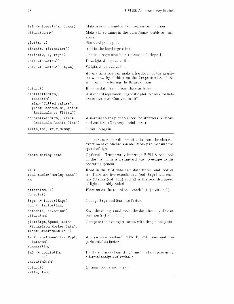
62 S-PLUS: An Introductory Session
lrf <- loess(y~x, dummy) Make a nonparametric local regression function.
attach(dummy) Make the columns in the data frame visible as vari-ables.
plot(x, y) Standard point plot.
lines(x, fitted(lrf)) Add in the local regression.
abline(0, 1, lty=3) The true regression line: (intercept 0, slope 1).
abline(coef(fm)) Unweighted regression line.
abline(coef(fm1),lty=4) Weighted regression line.
At any time you can make a hardcopy of the graph-ics window by clicking on the Graph section of thewindow and selecting the Print option.
detach() Remove data frame from the search list.
plot(fitted(fm),
resid(fm),
xlab="Fitted values",
ylab="Residuals", main=
"Residuals vs Fitted")
A standard regression diagnostic plot to check for het-eroscedasticity. Can you see it?
qqnorm(resid(fm), main=
"Residuals Rankit Plot")
A normal scores plot to check for skewness, kurtosisand outliers. (Not very useful here.)
rm(fm,fm1,lrf,x,dummy) Clean up again.
The next section will look at data from the classicalexperiment of Michaelson and Morley to measure thespeed of light.
!more morley.data Optional. Temporarily interrupt S-PLUS and lookat the �le. This is a standard way to escape to theoperating system.
mm <-
read.table("morley.data")
mm
Read in the MM data as a data frame, and look atit. There are �ve experiments (col. Expt) and eachhas 20 runs (col. Run) and sl is the recorded speedof light, suitably coded.
attach(mm, 1)
objects()
Place mm on the top of the search list, (position 1).
Expt <- factor(Expt)
Run <- factor(Run)
Change Expt and Run into factors.
detach(1, save="mm")
attach(mm)
Save the changes and make the data frame visible atposition 2 (the default).
plot(Expt,Speed, main=
"Michaelson Morley Data",
xlab="Experiment No.")
Compare the �ve experiments with simple boxplots.
fm <- aov(Speed~Run+Expt,
data=mm)
summary(fm)
Analyse as a randomized block, with `runs' and `ex-periments' as factors.
fm0 <- update(fm,
.~.-Run)
anova(fm0,fm)
Fit the sub-model omitting `runs', and compare usinga formal analysis of variance.
detach()
rm(fm, fm0)
Cleanup before moving on.

S-PLUS: An Introductory Session 63
We now look at some more graphical features: con-tour and 3�dimensional perspective plots.
x <- seq(-pi, pi, len=50)
y <- x
x is a vector of 50 equally spaced values in �� � x ��. y is the same.
f <- outer(x, y,
function(x,y)
cos(y)/(1+x*2))
f is a square matrix, with rows and columns indexedby x and y respectively, of values of the functioncos(y)=(1 + x2).
oldpar <- par()
par(pty="s")
Save the plotting parameters and set the plotting re-gion to \square".
contour(x, y, f)
contour(x, y, f,
nint=15, add=T)
Make a contour map of f ; add in more lines for moredetail.
fa <- (f-t(f))/2 fa is the \asymmetric part" of f . (t() is transpose).
contour(x, y, fa, nint=15) Make a contour, and
par(oldpar) restore the old graphics parameters.
persp(x, y, f)
persp(x, y, fa)
image(x, y, f)
image(x, y, fa)
Make some pretty perspective and high density imageplots, (of which you can get hardcopies if you wish)
objects(); rm(x,y,f,fa) and clean up before moving on.
th <- seq(-pi, pi,
len=100)
z <- exp(1i*th)
S-PLUS can do complex arithmetic, also. 1i is usedfor the complex number i
par(pty="s")
plot(z, type="l")
Plotting complex arguments means plot imaginaryversus real parts. This should be a circle.
w <- rnorm(100) +
rnorm(100)*1i
Suppose we want to sample points within the unit cir-cle. One method would be to take complex numberswith standard normal real and imaginary parts {
w <- ifelse(Mod(w) > 1,
1/w, w)
and to map any outside the circle onto their recipro-cal.
plot(w, xlim=c(-1,1),
ylim=c(-1,1), pch="+",
xlab="x", ylab="y")
lines(z)
All points are inside the unit circle, but the distribu-tion is not uniform.
w <- sqrt(runif(100))*
exp(2*pi*runif(100)*1i)
plot(w, xlim=c(-1,1),
ylim=c(-1,1), pch="+",
xlab="x", ylab="y")
lines(z)
The second method uses the uniform distribution.The points should now look more evenly spaced overthe disc.
rm(th,w,z) Cleanup again.
par(oldpar) Restore standard graphics parameters.
butterfly() An old favourite. Take a hardcopy if you wish.
rm(oldpar) Cleanup again.
q() Quit the S-PLUS program.
> and return to Unix.
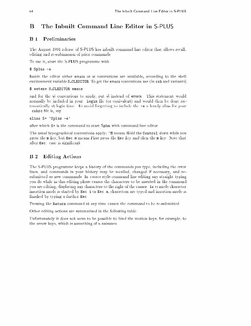
64 The Inbuilt Command Line Editor in S-PLUS
B The Inbuilt Command Line Editor in S-PLUS
B.1 Preliminaries
The August 1991 release of S-PLUS has inbuilt command line editor that allows recall,editing and re-submission of prior commands.
To use it, start the S-PLUS programme with
$ Splus -e
Inside the editor either emacs or vi conventions are available, according to the shellenvironment variable S CLEDITOR. To get the emacs conventions use (in csh and variants)
$ setenv S CLEDITOR emacs
and for the vi conventions to apply, put vi instead of emacs. This statement wouldnormally be included in your .login �le (or equivalent) and would then be done au-tomatically at login time. To avoid forgetting to include the -e a handy alias for your.cshrc �le is, say
alias S+ 'Splus -e'
after which S+ is the command to start Splus with command line editor.
The usual typographical conventions apply: ^M means Hold the Control down while youpress the m key, but Esc m means First press the Esc key and then the m key. Note thatafter Esc case is signi�cant.
B.2 Editing Actions
The S-PLUS programme keeps a history of the commands you type, including the errorlines, and commands in your history may be recalled, changed if necessary, and re-submitted as new commands. In emacs style command line editing any straight typingyou do while in this editing phase causes the characters to be inserted in the commandyou are editing, displacing any characters to the right of the cursor. In vi mode characterinsertion mode is started by Esc i or Esc a, characters are typed and insertion mode is�nished by typing a further Esc .
Pressing the Return command at any time causes the command to be re-submitted.
Other editing actions are summarised in the following table.
Unfortunately it does not seem to be possible to bind the motion keys, for example, tothe arrow keys, which is something of a nuisance.

B.3 Command Line Editor Summary 65
B.3 Command Line Editor Summary
1. Command recall and vertical motion emacs style vi style
Go to the previous command (backwards in the history) ^P Esc k
Go to the next command (forwards in the history) ^N Esc j
Find the last command with the text string in it ^R text Esc ? text
2. Horizontal motion of the cursor
Go to the beginning of the command ^A Esc ^
Go to the end of the line ^E Esc $
Go back one word Esc b Esc b
Go forward one word Esc f Esc w
Go back one character ^B Esc h
Go forward one character ^F Esc l
3. Editing and re-submission
Insert text at the cursor text Esc i text Esc
Append text after cursor ^Ftext Esc a text Esc
Delete the previous character (left of the cursor) Delete Esc shift-x
Delete the character under the cursor ^D Esc x
Delete rest of the word under the cursor, and `save' it Esc d Esc dw
Delete from cursor to end of command, and `save' it ^K Esc shift-d
Insert (yank) the last `saved' text here ^Y Esc shift-y
Transpose the character under the cursor with the next ^T Esc xp
Change the rest of the word to lower case Esc l
Change the rest of the word to capitals (upper case) Esc c
Re-submit the command to S-PLUS Return Return
NOTE: With vi style commands the Esc need only be issued before the �rst recallcommand, and to terminate insert and append commands, as is usual in vi.
The �nal Return terminates the command line editing sequence for commands of eitherstyle.

66 Exercises
C Exercises
C.1 The Cloud Point Data
Source: Draper & Smith, Applied Regression Analysis, p. 162Category: Polynomial regression. Simple plots.
Description
The cloud point of a liquid is a measure of the degree of crystalization in a stock thatcan be measured by the refractive index. It has been suggested that the percentage of I8in the base stock is an excellent predictor of cloud point using the second or third ordermodel:
Y = �0 + �1x+ �2x2 + �3x
3 + E; E � N(0; �2)
Data
The following data was collected on stocks with known percentage of I8:
I8% Cloud Point I8% Cloud Point I8% Cloud Point I8% Cloud Point
0 21.9 2 26.1 5 28.9 8 31.4
0 22.1 3 26.8 6 29.8 8 31.5
0 22.8 3 27.3 6 30.0 9 31.8
1 24.5 4 28.2 6 30.3 10 33.1
2 26.0 4 28.5 7 30.4
The data may be read from �le cloud.data in a form suitable to construct a data frame.
C.2 The Janka Hardness Data
Source: E. J. Williams: Regression Analysis, Wiley, 1959.Category: Polynomial regression. Transformations.
Description
The Janka hardness is an important structural property of Australian timbers, which isdi�cult to measure. It is, however, related to the density of the timber, which is relativelyeasy to measure. A low degree polynomial regression is suggested as appropriate.
Y = �0 + �1x+ �2x2 + � � �+ E
where Y is the hardness and x the density.
Data
The following data comes from samples of 36 Australian Eucalypt hardwoods.

C.3 The Tuggeranong House Price Data 67
D H D H D H D H D H D H
24.7 484 30.3 587 39.4 1210 42.9 1270 53.4 1880 59.8 1940
24.8 427 32.7 704 39.9 989 45.8 1180 56.0 1980 66.0 3260
27.3 413 35.6 979 40.3 1160 46.9 1400 56.5 1820 67.4 2700
28.4 517 38.5 914 40.6 1010 48.2 1760 57.3 2020 68.8 2890
28.4 549 38.8 1070 40.7 1100 51.5 1710 57.6 1980 69.1 2740
29.0 648 39.3 1020 40.7 1130 51.5 2010 59.2 2310 69.1 3140
The data may be read as a data frame from �le janka.data.
C.3 The Tuggeranong House Price Data
Source: Dr Ray Correll, Personal communicationCategory: Multiple regression, coplots.
Description
Before buying a house in Tuggeranong in February, 1987, a cautious potential house-holder collected some data on houses on the market. The data for 20 such houses isshown in the table and is available as the �le house.dat. The variables collected are,in order, price, total oor area, block area, number of main rooms, age of house andwhether or not the house was centrally heated.
Data
The data is given in Table 5 and is available as the �le house.data.
C.4 Yorke Penninsula Wheat Data
Source: K. W. Morris (private communication)Category: Multiple regression.
Description
The annual yield of wheat in a marginal wheat growing district on the Yorke Penninsula,South Australia, together with the rainfall for the three growing months, for the years1931{1955. The year itself is potentially a surrogate predictor to allow for improvementsin varieties and farm practice. Yield is in bushels per acre, and rainfall is in inches.
Data
The data is given in Table 6 and may be read as a data frame from �le sawheat.data.
C.5 The Iowa Wheat Yield Data
Source: CAED Report, 1964. Quoted in Draper & Smith.Category: Multiple regression; diagnostics.

68 Exercises
Price ($000s) Floor (m2) Block (m2) Rooms Age (years) Cent. Heat.
52.00 111.0 830 5 6.2 no
54.75 128.0 710 5 7.5 no
57.50 101.0 1000 5 4.2 no
57.50 131.0 690 6 8.8 no
59.75 93.0 900 5 1.9 yes
62.50 112.0 640 6 5.2 no
64.75 137.6 700 6 6.6 yes
67.25 148.5 740 6 2.3 no
67.50 113.5 660 6 6.1 no
69.75 152.0 645 7 9.2 no
70.00 121.5 730 5 4.3 yes
75.50 141.0 730 7 4.3 no
77.50 124.0 670 6 1.0 yes
77.50 153.5 795 7 7.0 yes
81.25 149.0 900 6 3.6 yes
82.50 135.0 810 6 1.7 yes
86.25 162.0 930 6 1.2 yes
87.50 145.0 825 6 0.0 yes
88.00 172.0 950 7 2.3 yes
92.00 170.5 870 7 0.7 yes
Table 5: The Tuggeranong house price data
Description
The data gives the pre-season and three growing months' precipitation, the mean tem-peratures for the three growing months and harvest month, the year, and the yield ofwheat for the USA state of Iowa, for the years 1930{1962.
Data
The data is given in Table 7 and may be read as a data frame from �le iowheat.data.
C.6 The Gasoline Yield Data
Source: Estimate gasoline yields from crudes
by Nilon H. Prater, Petroleum Re�ner, 35, #5.Category: Analysis of variance, covariance, and multiple regression.
Modern regression.
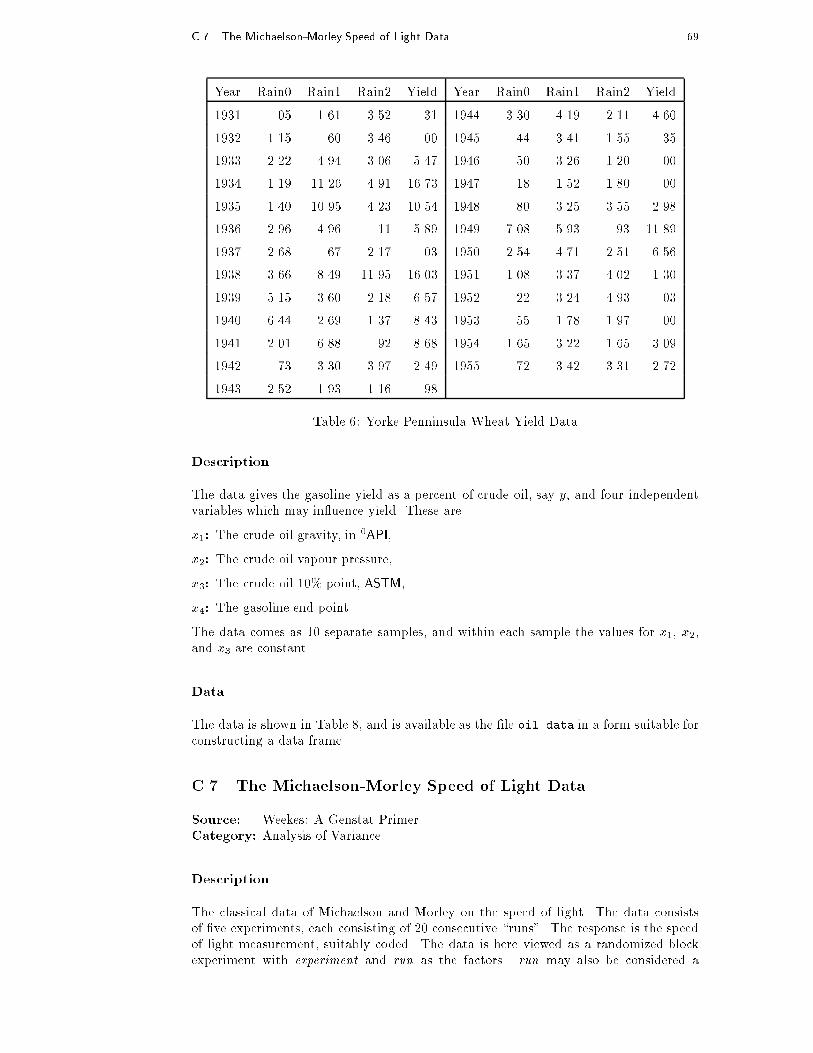
C.7 The Michaelson-Morley Speed of Light Data 69
Year Rain0 Rain1 Rain2 Yield Year Rain0 Rain1 Rain2 Yield
1931 .05 1.61 3.52 .31 1944 3.30 4.19 2.11 4.60
1932 1.15 .60 3.46 .00 1945 .44 3.41 1.55 .35
1933 2.22 4.94 3.06 5.47 1946 .50 3.26 1.20 .00
1934 1.19 11.26 4.91 16.73 1947 .18 1.52 1.80 .00
1935 1.40 10.95 4.23 10.54 1948 .80 3.25 3.55 2.98
1936 2.96 4.96 .11 5.89 1949 7.08 5.93 .93 11.89
1937 2.68 .67 2.17 .03 1950 2.54 4.71 2.51 6.56
1938 3.66 8.49 11.95 16.03 1951 1.08 3.37 4.02 1.30
1939 5.15 3.60 2.18 6.57 1952 .22 3.24 4.93 .03
1940 6.44 2.69 1.37 8.43 1953 .55 1.78 1.97 .00
1941 2.01 6.88 .92 8.68 1954 1.65 3.22 1.65 3.09
1942 .73 3.30 3.97 2.49 1955 .72 3.42 3.31 2.72
1943 2.52 1.93 1.16 .98
Table 6: Yorke Penninsula Wheat Yield Data
Description
The data gives the gasoline yield as a percent of crude oil, say y, and four independentvariables which may in uence yield. These are
x1: The crude oil gravity, in0API,
x2: The crude oil vapour pressure,
x3: The crude oil 10% point, ASTM,
x4: The gasoline end point.
The data comes as 10 separate samples, and within each sample the values for x1, x2,and x3 are constant.
Data
The data is shown in Table 8, and is available as the �le oil.data in a form suitable forconstructing a data frame.
C.7 The Michaelson-Morley Speed of Light Data
Source: Weekes: A Genstat Primer.Category: Analysis of Variance.
Description
The classical data of Michaelson and Morley on the speed of light. The data consistsof �ve experiments, each consisting of 20 consecutive \runs". The response is the speedof light measurement, suitably coded. The data is here viewed as a randomized blockexperiment with experiment and run as the factors. run may also be considered a

70 Exercises
Year Rain0 Temp1 Rain1 Temp2 Rain2 Temp3 Rain3 Temp4 Yield
1930 17.75 60.2 5.83 69.0 1.49 77.9 2.42 74.4 34.0
1931 14.76 57.5 3.83 75.0 2.72 77.2 3.30 72.6 32.9
1932 27.99 62.3 5.17 72.0 3.12 75.8 7.10 72.2 43.0
1933 16.76 60.5 1.64 77.8 3.45 76.4 3.01 70.5 40.0
1934 11.36 69.5 3.49 77.2 3.85 79.7 2.84 73.4 23.0
1935 22.71 55.0 7.00 65.9 3.35 79.4 2.42 73.6 38.4
1936 17.91 66.2 2.85 70.1 0.51 83.4 3.48 79.2 20.0
1937 23.31 61.8 3.80 69.0 2.63 75.9 3.99 77.8 44.6
1938 18.53 59.5 4.67 69.2 4.24 76.5 3.82 75.7 46.3
1939 18.56 66.4 5.32 71.4 3.15 76.2 4.72 70.7 52.2
1940 12.45 58.4 3.56 71.3 4.57 76.7 6.44 70.7 52.3
1941 16.05 66.0 6.20 70.0 2.24 75.1 1.94 75.1 51.0
1942 27.10 59.3 5.93 69.7 4.89 74.3 3.17 72.2 59.9
1943 19.05 57.5 6.16 71.6 4.56 75.4 5.07 74.0 54.7
1944 20.79 64.6 5.88 71.7 3.73 72.6 5.88 71.8 52.0
1945 21.88 55.1 4.70 64.1 2.96 72.1 3.43 72.5 43.5
1946 20.02 56.5 6.41 69.8 2.45 73.8 3.56 68.9 56.7
1947 23.17 55.6 10.39 66.3 1.72 72.8 1.49 80.6 30.5
1948 19.15 59.2 3.42 68.6 4.14 75.0 2.54 73.9 60.5
1949 18.28 63.5 5.51 72.4 3.47 76.2 2.34 73.0 46.1
1950 18.45 59.8 5.70 68.4 4.65 69.7 2.39 67.7 48.2
1951 22.00 62.2 6.11 65.2 4.45 72.1 6.21 70.5 43.1
1952 19.05 59.6 5.40 74.2 3.84 74.7 4.78 70.0 62.2
1953 15.67 60.0 5.31 73.2 3.28 74.6 2.33 73.2 52.9
1954 15.92 55.6 6.36 72.9 1.79 77.4 7.10 72.1 53.9
1955 16.75 63.6 3.07 67.2 3.29 79.8 1.79 77.2 48.4
1956 12.34 62.4 2.56 74.7 4.51 72.7 4.42 73.0 52.8
1957 15.82 59.0 4.84 68.9 3.54 77.9 3.76 72.9 62.1
1958 15.24 62.5 3.80 66.4 7.55 70.5 2.55 73.0 66.0
1959 21.72 62.8 4.11 71.5 2.29 72.3 4.92 76.3 64.2
1960 25.08 59.7 4.43 67.4 2.76 72.6 5.36 73.2 63.2
1961 17.79 57.4 3.36 69.4 5.51 72.6 3.04 72.4 75.4
1962 26.61 66.6 3.12 69.1 6.27 71.6 4.31 72.5 76.0
Table 7: The Iowa Historical Wheat Yield Data
quantitative variate to account for linear (or polynomial) changes in the measurementover the course of a single experiment.
Data
The data is given in Table 9 and may be read as a data frame from �le morley.data ina form suitable for constructing a data frame.
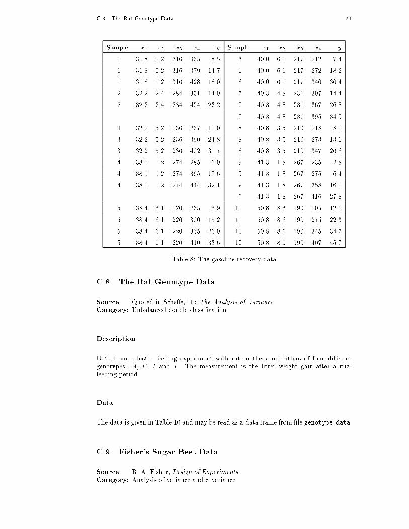
C.8 The Rat Genotype Data 71
Sample x1 x2 x3 x4 y Sample x1 x2 x3 x4 y
1 31.8 0.2 316 365 8.5 6 40.0 6.1 217 212 7.4
1 31.8 0.2 316 379 14.7 6 40.0 6.1 217 272 18.2
1 31.8 0.2 316 428 18.0 6 40.0 6.1 217 340 30.4
2 32.2 2.4 284 351 14.0 7 40.3 4.8 231 307 14.4
2 32.2 2.4 284 424 23.2 7 40.3 4.8 231 367 26.8
7 40.3 4.8 231 395 34.9
3 32.2 5.2 236 267 10.0 8 40.8 3.5 210 218 8.0
3 32.2 5.2 236 360 24.8 8 40.8 3.5 210 273 13.1
3 32.2 5.2 236 402 31.7 8 40.8 3.5 210 347 26.6
4 38.1 1.2 274 285 5.0 9 41.3 1.8 267 235 2.8
4 38.1 1.2 274 365 17.6 9 41.3 1.8 267 275 6.4
4 38.1 1.2 274 444 32.1 9 41.3 1.8 267 358 16.1
9 41.3 1.8 267 416 27.8
5 38.4 6.1 220 235 6.9 10 50.8 8.6 190 205 12.2
5 38.4 6.1 220 300 15.2 10 50.8 8.6 190 275 22.3
5 38.4 6.1 220 365 26.0 10 50.8 8.6 190 345 34.7
5 38.4 6.1 220 410 33.6 10 50.8 8.6 190 407 45.7
Table 8: The gasoline recovery data
C.8 The Rat Genotype Data
Source: Quoted in Sche�e, H.: The Analysis of Variance
Category: Unbalanced double classi�cation.
Description
Data from a foster feeding experiment with rat mothers and litters of four di�erentgenotypes: A, F , I and J . The measurement is the litter weight gain after a trialfeeding period.
Data
The data is given in Table 10 and may be read as a data frame from �le genotype.data.
C.9 Fisher's Sugar Beet Data
Source: R. A. Fisher, Design of Experiments.Category: Analysis of variance and covariance.

72 Exercises
Runs 1{10 Runs 11{20
E1 E2 E3 E4 E5 E1 E2 E3 E4 E5
850 960 880 890 890 1000 830 880 910 870
740 940 880 810 840 980 790 910 920 870
900 960 880 810 780 930 810 850 890 810
1070 940 860 820 810 650 880 870 860 740
930 880 720 800 760 760 880 840 880 810
850 800 720 770 810 810 830 840 720 940
950 850 620 760 790 1000 800 850 840 950
980 880 860 740 810 1000 790 840 850 800
980 900 970 750 820 960 760 840 850 810
880 840 950 760 850 960 800 840 780 870
Table 9: The Michaelson-Morley speed of light data
Description
A classical 3�23 randomized block experiment in four blocks of size 24. The response isthe total weight of sugarbeet roots o� the plot, but this is accompanied by the numberof roots measured. The suggestion is that number of roots should be a covariate to allowfor varying plot size.
The factors are Variety. (3 levels, a, b and c), and N, P and K each at 2 levels, presentor absent.
Data
The data is given in Table 11 and may be read from the �le sugar.data in a formsuitable to construct a data frame.
C.10 A Barley Split Plot Field Trial.
Source: Unknown. Traditional data.Category: Multistratum analysis of variance.
Description
An experiment involving barley varieties and manure (nitrogen) was conducted in 6blocks of 3 whole plots.
Each whole plot was divided into 4 subplots. Three varieties of barley were used inthe experiment with one variety being sown in each whole plot, while the four levels ofmanure (0, 0.01, 0.02, and 0.04 tons per acre) were used, one level in each of the foursubplots of each whole plot. In the above table Vi denotes the ith variety and Nj denotesthe jth level of nitrogen.
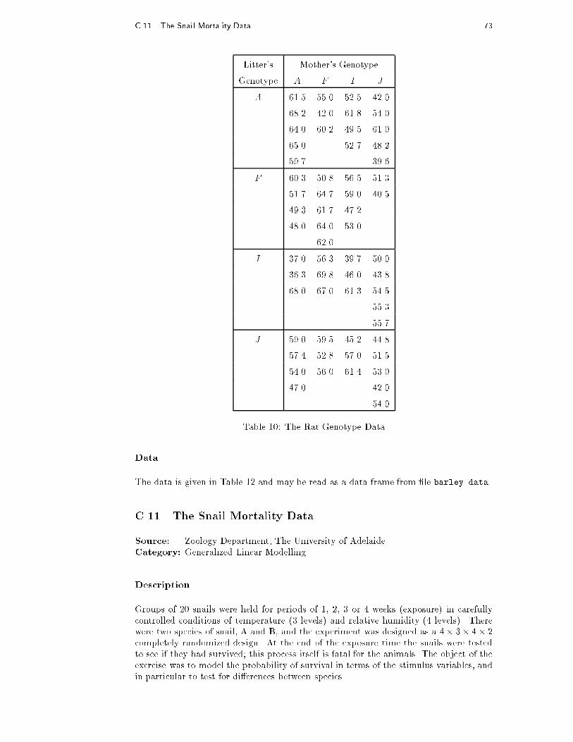
C.11 The Snail Mortality Data 73
Litter's Mother's Genotype
Genotype A F I J
A 61.5 55.0 52.5 42.0
68.2 42.0 61.8 54.0
64.0 60.2 49.5 61.0
65.0 52.7 48.2
59.7 39.6
F 60.3 50.8 56.5 51.3
51.7 64.7 59.0 40.5
49.3 61.7 47.2
48.0 64.0 53.0
62.0
I 37.0 56.3 39.7 50.0
36.3 69.8 46.0 43.8
68.0 67.0 61.3 54.5
55.3
55.7
J 59.0 59.5 45.2 44.8
57.4 52.8 57.0 51.5
54.0 56.0 61.4 53.0
47.0 42.0
54.0
Table 10: The Rat Genotype Data
Data
The data is given in Table 12 and may be read as a data frame from �le barley.data.
C.11 The Snail Mortality Data
Source: Zoology Department, The University of Adelaide.Category: Generalized Linear Modelling.
Description
Groups of 20 snails were held for periods of 1, 2, 3 or 4 weeks (exposure) in carefullycontrolled conditions of temperature (3 levels) and relative humidity (4 levels). Therewere two species of snail, A and B, and the experiment was designed as a 4� 3� 4 � 2completely randomized design. At the end of the exposure time the snails were testedto see if they had survived; this process itself is fatal for the animals. The object of theexercise was to model the probability of survival in terms of the stimulus variables, andin particular to test for di�erences between species.

74 Exercises
Block 1 Block 2 Block 3 Block 4
V N P K No Wt No Wt No Wt No Wt
a � � � 124 162 133 162 114 127 127 158
a � � k 131 152 161 164 130 141 145 188
a � p � 115 173 134 175 134 142 109 162
a � p k 126 140 133 158 106 148 132 160
a n � � 136 184 134 178 127 168 139 199
a n � k 134 112 156 193 101 171 138 191
a n p � 132 190 104 166 119 157 132 193
a n p k 120 175 147 155 107 139 148 192
b � � � 145 133 147 130 139 138 127 128
b � � k 156 117 152 137 107 121 147 147
b � p � 152 140 138 101 125 124 120 143
b � p k 137 127 145 132 125 132 143 139
b n � � 124 163 138 159 140 166 159 174
b n � k 136 143 142 144 133 142 148 159
b n p � 140 168 142 150 133 118 138 157
b n p k 146 144 135 160 138 155 140 153
c � � � 113 122 138 132 119 123 127 146
c � � k 91 107 149 171 118 142 129 151
c � p � 123 118 139 142 127 120 124 138
c � p k 129 140 126 115 129 130 142 152
c n � � 121 118 141 152 127 149 127 165
c n � k 126 148 128 152 107 147 110 136
c n p � 103 112 144 175 102 152 143 173
c n p k 120 162 125 160 129 173 137 185
Table 11: Fisher's sugar beet data
The data is unusual in that in most cases fatalities during the experiment were fairlysmall.
Data
The data is given in Table 13 and may be read as a data frame from �le snails.data.
C.12 The Kalythos Blindness Data
Source: S. D. Silvey: Statistical Inference. (Fictitious?)Category: Generalized linear modelling

C.12 The Kalythos Blindness Data 75
Block Variety N1 N2 N3 N4 Block Variety N1 N2 N3 N4
V1 111 130 157 174 V1 74 89 81 122
I V2 117 114 161 141 IV V2 64 103 132 133
V3 105 140 118 156 V3 70 89 104 117
V1 61 91 97 100 V1 62 90 100 116
II V2 70 108 126 149 V V2 80 82 94 126
V3 96 124 121 144 V3 63 70 109 99
V1 68 64 112 86 V1 53 74 118 113
III V2 60 102 89 96 VI V2 89 82 86 104
V3 89 129 132 124 V3 97 99 119 121
Table 12: A split plot Barley �eld trial
Relative Humidity60.0% 65.8% 70.5% 75.8%
Temperature Temperature Temperature TemperatureSpecies Exposure 10 15 20 10 15 20 10 15 20 10 15 20
A 1 0 0 0 0 0 0 0 0 0 0 0 0
2 0 1 1 0 1 0 0 0 0 0 0 0
3 1 4 5 0 2 4 0 2 3 0 1 2
4 7 7 7 4 4 7 3 3 5 2 3 3
B 1 0 0 0 0 0 0 0 0 0 0 0 0
2 0 3 2 0 2 1 0 0 1 1 0 1
3 7 11 11 4 5 9 2 4 6 2 3 5
4 12 14 16 10 12 12 5 7 9 4 5 7
Table 13: The snail mortality data
Description
On the Greek island of Kalythos the male inhabitants su�er from a congenital eye disease,the e�ects of which become more marked with increasing age. Samples of islander malesof various ages were tested for blindness and the results recorded.
Data
Age: 20 35 45 55 70
No. tested: 50 50 50 50 50
No. blind: 6 17 26 37 44
Table 14: The Kalythos blindness data
The data is given in Table 14 and may be read as a data frame from �le kalythos.data.

76 Exercises
Problems
C.13 The Stormer Viscometer Data
Source: E. J. Williams: Regression Analysis, Wiley, 1959Category: Nonlinear regression, special regression.
Description
The stormer viscometer measures the viscosity of a uid by measuring the time takenfor an inner cylinder in the mechanism to perform a �xed number of revolutions inresponse to an actuating weight. The viscometer is calibrated by measuring the timetaken with varying weights while the mechanism is suspended in uids of accuratelyknown viscosity. The data comes from such a calibration, and theoretical considerationssuggest a nonlinear relationship between time, weight and viscosity of the form
T =�vi
wi � �+Ei
where � and � are unknown parameters to be estimated.
Data
Weight
Viscosity 20 50 100
14.7 35.6 17.6
27.5 54.3 24.3
42.0 75.6 31.4
75.7 121.2 47.2 24.6
89.7 150.8 58.3 30.0
146.6 229.0 85.6 41.7
158.3 270.0 101.1 50.3
161.1 92.2 45.1
298.3 187.2 89.0
86.5
Table 15: The Stormer viscometer calibration data
The data is given in Table 15 and may be read as a data frame from �le stormer.data.
C.14 The Chlorine availability data
Source: Draper & Smith, Applied Regression Analysis, (adapted).Category: Nonlinear regression

C.15 The Saturated Steam Pressure Data 77
Description
The following set of industrial chemical data shows the amount of chlorine available ina certain product at various times of testing after manufacture. A nonlinear regressionmodel for the chlorine decay of the form
Y = �0 + �1 exp(��t)
has been suggested on theoretical grounds, with Y the amount remaining at time t.
Data
Weeks Percent available Weeks Percent available Weeks Percent available
8 49, 49 20 42, 43, 42 32 40, 41
10 47, 47, 48, 48 22 40, 41, 41 34 40
12 43, 45, 46, 46 24 40, 40, 42 36 38, 41
14 43, 43, 45 26 40, 41, 41 38 40, 40
16 43, 43, 44 28 40, 41 40 39
18 45, 46 30 38, 40, 40 42 39
Table 16: The Chlorine availability data.
The data is given in Table 16 and may be read as a data frame from �le chlorine.data.
C.15 The Saturated Steam Pressure Data
Source: Quoted in Draper & Smith: Applied Regression Analysis: : :
Category: Nonlinear regression.
Description
The data gives the temperature (0C) and pressure (Pascals) in a saturated steam drivenexperimental device. The relationship between pressure, Y , and temperature, t, in sat-urated steam can be written as
Y = � exp
��t
+ t
�+E
However a more realistic model may have the experimental errors multiplicative ratherthan additive, in which case an analysis in the log scale using the model
logY = log�+
��t
+ t
�+E
may be more appropriate.
Data
The data is given in Table 17 and may be read as a data frame from �le steam.data.
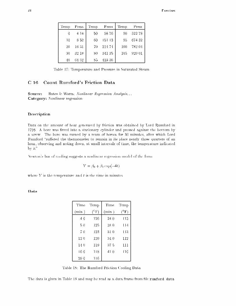
78 Exercises
Temp Press Temp Press Temp Press
0 4.14 50 98.76 90 522.78
10 8.52 60 151.13 95 674.32
20 16.31 70 224.74 100 782.04
30 32.18 80 341.35 105 920.01
40 64.62 85 423.36
Table 17: Temperature and Pressure in Saturated Steam
C.16 Count Rumford's Friction Data
Source: Bates & Watts: Nonlinear Regression Analysis: : :
Category: Nonlinear regression
Description
Data on the amount of heat generated by friction was obtained by Lord Rumford in1798. A bore was �tted into a stationary cylinder and pressed against the bottom bya screw. The bore was turned by a team of horses for 30 minutes, after which LordRumford \su�ered the thermometer to remain in its place nearly three quarters of anhour, observing and noting down, at small intervals of time, the temperature indicatedby it".
Newton's law of cooling suggests a nonlinear regression model of the form
Y = �0 + �1 exp(��t)
where Y is the temperature and t is the time in minutes.
Data
Time Temp Time Temp
(min.) (0F) (min.) (0F)
4.0 126 24.0 115
5.0 125 28.0 114
7.0 123 31.0 113
12.0 120 34.0 112
14.0 119 37.5 111
16.0 118 41.0 110
20.0 116
Table 18: The Rumford Friction Cooling Data
The data is given in Table 18 and may be read as a data frame from �le rumford.data.

C.17 The Jelly�sh Data. 79
C.17 The Jelly�sh Data.
Source: Interactive Statistics, Ed. Don McNeil.Category: Bivariate, two sample data.
Description
Two samples of jelly�sh, from Danger Island and Salamander Bay respectively, weremeasured for length and width.
Data
Danger Island Salamander Bay
Width Length Width Length Width Length Width Length
6.0 9.0 11.0 13.0 12.0 14.0 16.0 20.0
6.5 8.0 11.0 14.0 13.0 17.0 16.0 20.0
6.5 9.0 11.0 14.0 14.0 16.5 16.0 21.0
7.0 9.0 12.0 13.0 14.0 19.0 16.5 19.0
7.0 10.0 13.0 14.0 15.0 16.0 17.0 20.0
7.0 11.0 14.0 16.0 15.0 17.0 18.0 19.0
8.0 9.5 15.0 16.0 15.0 18.0 18.0 19.0
8.0 10.0 15.0 16.0 15.0 18.0 18.0 20.0
8.0 10.0 15.0 19.0 15.0 19.0 19.0 20.0
8.0 11.0 16.0 16.0 15.0 21.0 19.0 22.0
9.0 11.0 16.0 18.0 20.0 22.0
10.0 13.0 16.0 19.0 21.0 21.0
Table 19: The Jelly�sh data { Danger Island and Salamander Bay
The data is given in Table 19 and may be read as a data frame from �le jellyfish.data.
C.18 Archaelogical Pottery Data
Source: Tubb, A. et al. Archaeometry, 22, 153{171, (1980)Category: Multivariate analysis
Description
The data arises from a chemical analysis of 26 samples of pottery found at Romano-British kiln sites in Wales, Gwent and the New Forest. The variables describe thecomposition, in terms of various metals, and are expressed as percentages of the oxidesof the metals.
The metals are aluminium, iron, magnesium, calcium and sodium and the sites are
L: Llanederyn, C: Caldicot I: Island Thorns A: Ashley Rails
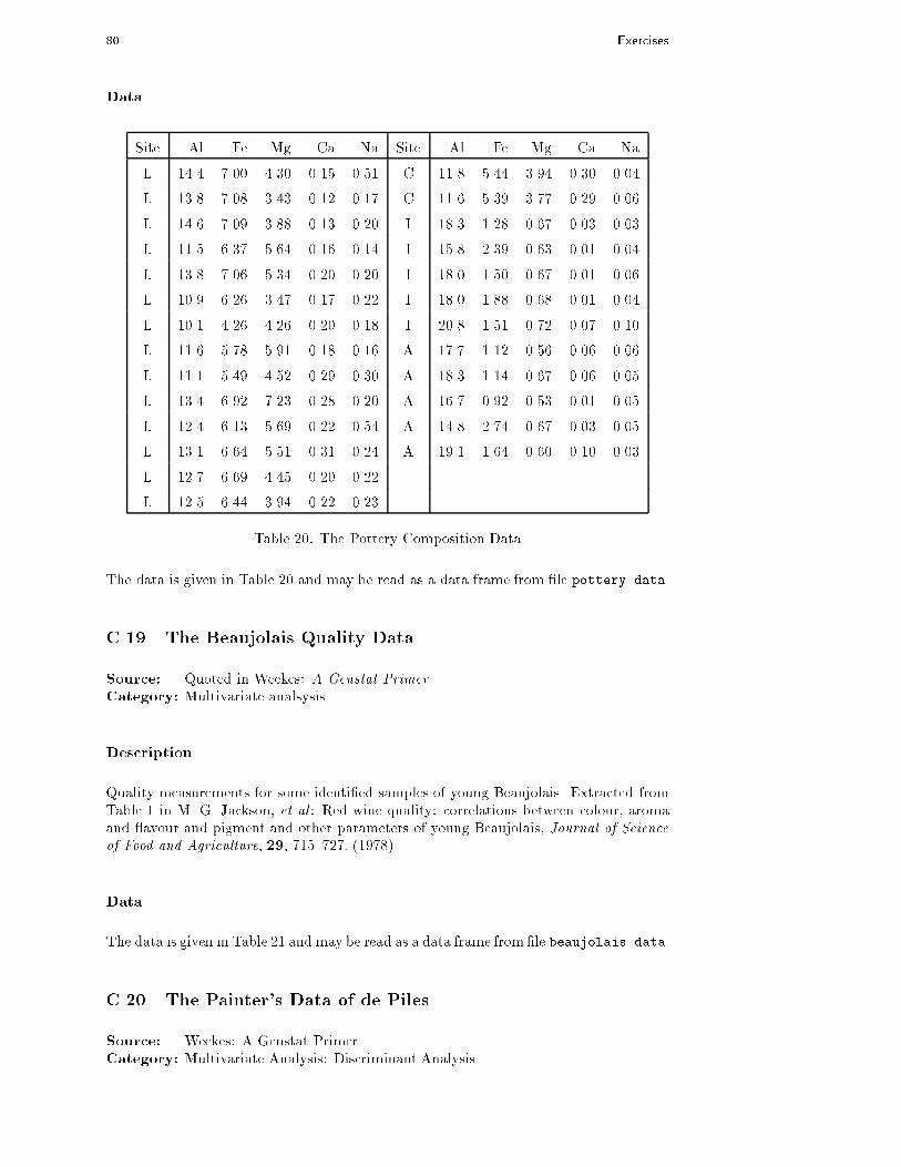
80 Exercises
Data
Site Al Fe Mg Ca Na Site Al Fe Mg Ca Na
L 14.4 7.00 4.30 0.15 0.51 C 11.8 5.44 3.94 0.30 0.04
L 13.8 7.08 3.43 0.12 0.17 C 11.6 5.39 3.77 0.29 0.06
L 14.6 7.09 3.88 0.13 0.20 I 18.3 1.28 0.67 0.03 0.03
L 11.5 6.37 5.64 0.16 0.14 I 15.8 2.39 0.63 0.01 0.04
L 13.8 7.06 5.34 0.20 0.20 I 18.0 1.50 0.67 0.01 0.06
L 10.9 6.26 3.47 0.17 0.22 I 18.0 1.88 0.68 0.01 0.04
L 10.1 4.26 4.26 0.20 0.18 I 20.8 1.51 0.72 0.07 0.10
L 11.6 5.78 5.91 0.18 0.16 A 17.7 1.12 0.56 0.06 0.06
L 11.1 5.49 4.52 0.29 0.30 A 18.3 1.14 0.67 0.06 0.05
L 13.4 6.92 7.23 0.28 0.20 A 16.7 0.92 0.53 0.01 0.05
L 12.4 6.13 5.69 0.22 0.54 A 14.8 2.74 0.67 0.03 0.05
L 13.1 6.64 5.51 0.31 0.24 A 19.1 1.64 0.60 0.10 0.03
L 12.7 6.69 4.45 0.20 0.22
L 12.5 6.44 3.94 0.22 0.23
Table 20: The Pottery Composition Data
The data is given in Table 20 and may be read as a data frame from �le pottery.data.
C.19 The Beaujolais Quality Data
Source: Quoted in Weekes: A Genstat Primer
Category: Multivariate analsysis
Description
Quality measurements for some identi�ed samples of young Beaujolais. Extracted fromTable 1 in M. G. Jackson, et al : Red wine quality: correlations between colour, aromaand avour and pigment and other parameters of young Beaujolais, Journal of Scienceof Food and Agriculture, 29, 715{727, (1978).
Data
The data is given in Table 21 and may be read as a data frame from�le beaujolais.data.
C.20 The Painter's Data of de Piles
Source: Weekes: A Genstat Primer.Category: Multivariate Analysis: Discriminant Analysis.

C.20 The Painter's Data of de Piles 81
Label OQ AC pH TSO Label OQ AC pH TSO
A 13.54 1.51 3.36 13.8 I 12.25 1.32 3.38 1.4
B 12.58 1.35 3.15 5.2 J 14.04 1.52 3.61 4.5
C 11.83 1.09 3.30 10.6 K 12.67 1.62 3.38 0.4
D 12.83 1.15 3.41 2.2 L 13.54 1.57 3.55 7.9
E 12.83 1.32 3.44 2.3 M 13.75 1.63 3.34 6.3
F 12.12 1.23 3.31 10.5 N 9.63 0.78 3.19 40.4
G 11.29 1.14 3.49 2.5 O 12.42 1.14 3.31 3.1
H 12.79 1.22 3.56 16.7
Table 21: Quality Measurements on Young Beaujolais Wine Samples
Description
The data shows the subjective assessment, on a 0{20 integer scale, of 54 classical painters.The painters were assessed on four characteristics: composition, drawing, colour andexpression. The data is due to the Eighteenth century art critic, de Piles.
The School to which a painter belongs is indicated by a letter code as follows:
A Renaissance E Lombard
B Mannerist F Sixteenth Century
C Seicento G Seventeenth Century
D Venetian H French
Data
The data is given in Table 22 and may be read as a data frame from �le painters.data.

82 Exercises
Composition Drawing Colour Expression School
Da Udine 10 8 16 3 ADa Vinci 15 16 4 14 A
Del Piombo 8 13 16 7 A
Del Sarto 12 16 9 8 AFr. Penni 0 15 8 0 A
Guilio Romano 15 16 4 14 A
Michelangelo 8 17 4 8 APerino del Vaga 15 16 7 6 A
Perugino 4 12 10 4 A
Raphael 17 18 12 18 A
F. Zucarro 10 13 8 8 B
Fr. Salviata 13 15 8 8 BParmigiano 10 15 6 6 B
Primaticcio 15 14 7 10 B
T. Zucarro 13 14 10 9 BVolterra 12 15 5 8 B
Barocci 14 15 6 10 CCortona 16 14 12 6 C
Josepin 10 10 6 2 C
L. Jordaens 13 12 9 6 C
Testa 11 15 0 6 C
Vanius 15 15 12 13 C
Bassano 6 8 17 0 D
Bellini 4 6 14 0 DGiorgione 8 9 18 4 D
Murillo 6 8 15 4 D
Palma Giovane 12 9 14 6 DPalma Vecchio 5 6 16 0 D
Pordenone 8 14 17 5 D
Tintoretto 15 14 16 4 D
Titian 12 15 18 6 D
Veronese 15 10 16 3 D
Albani 14 14 10 6 E
Caravaggio 6 6 16 0 E
Corregio 13 13 15 12 EDomenichino 15 17 9 17 E
Guercino 18 10 10 4 E
Lanfranco 14 13 10 5 EThe Carraci 15 17 13 13 E
Durer 8 10 10 8 F
Holbein 9 10 16 13 F
Pourbus 4 15 6 6 F
Van Leyden 8 6 6 4 F
Diepenbeck 11 10 14 6 G
J. Jordaens 10 8 16 6 GOtho Venius 13 14 10 10 G
Rembrandt 15 6 17 12 G
Rubens 18 13 17 17 GTeniers 15 12 13 6 G
Van Dyck 15 10 17 13 G
Bourdon 10 8 8 4 H
Le Brun 16 16 8 16 H
Le Suer 15 15 4 15 HPoussin 15 17 6 15 H
Table 22: The Subjective Assessment Data of de Piles