notes on (algebra based) physicsshajesh/tc/201608-siu-p203b/files/algebra... · notes on (algebra...

Notes on (algebra based) Physics

Prachi Parashar1 and K. V. Shajesh2

Department of Physics,

Southern Illinois University–Carbondale,

Carbondale, Illinois 62901, USA.

Last major update: May 20, 2016Last updated: September 13, 2017

These are notes prepared for the benefit of students enrolled in PHYS-203A and PHYS-203B, algebra basedintroductory physics courses for non-physics majors, at Southern Illinois University–Carbondale. The followingtextbooks were extensively used in this compilation.

1. (Assigned Textbook in Fall 2015)Physics, Ninth Edition,John D. Cutnell and Kenneth W. Johnson,John Wiley & Sons, Inc.

2. Fundamentals of physics, Fifth Edition,David Halliday, Robert Resnick, and Jearl Walker,John Wiley & Sons, Inc.

These notes were primarily written in the academic year of 2015. It will be updated periodically, and will evolveduring the semester. It is not a substitute for the assigned textbook for the course, but a supplement preparedas a study-guide.

1EMAIL: [email protected]: [email protected], URL: http://www.physics.siu.edu/~shajesh

http://www.physics.siu.edu/~shajesh

Contents

I Mechanics 7

1 Measurement 9

1.1 International System (SI) of units . . . . . . . . . . . . . . . . . . . . . . . . . . . . . . . . . . . . 9

1.2 Dimensional analysis . . . . . . . . . . . . . . . . . . . . . . . . . . . . . . . . . . . . . . . . . . . 9

1.3 Measurement . . . . . . . . . . . . . . . . . . . . . . . . . . . . . . . . . . . . . . . . . . . . . . . 11

2 Motion in one dimension 13

2.1 Motion . . . . . . . . . . . . . . . . . . . . . . . . . . . . . . . . . . . . . . . . . . . . . . . . . . . 13

2.2 Graphical analysis . . . . . . . . . . . . . . . . . . . . . . . . . . . . . . . . . . . . . . . . . . . . 14

2.3 Motion with constant acceleration . . . . . . . . . . . . . . . . . . . . . . . . . . . . . . . . . . . 15

3 Vector algebra 19

3.1 Vector . . . . . . . . . . . . . . . . . . . . . . . . . . . . . . . . . . . . . . . . . . . . . . . . . . . 19

3.2 Addition and subtraction of vectors . . . . . . . . . . . . . . . . . . . . . . . . . . . . . . . . . . . 20

3.3 Graphical method . . . . . . . . . . . . . . . . . . . . . . . . . . . . . . . . . . . . . . . . . . . . 21

4 Motion in two dimensions 23

4.1 Motion in 2D . . . . . . . . . . . . . . . . . . . . . . . . . . . . . . . . . . . . . . . . . . . . . . . 23

4.2 Projectile motion . . . . . . . . . . . . . . . . . . . . . . . . . . . . . . . . . . . . . . . . . . . . . 24

4.3 Galilean relativity . . . . . . . . . . . . . . . . . . . . . . . . . . . . . . . . . . . . . . . . . . . . 26

5 Newton’s laws of motion 29

5.1 Laws of motion . . . . . . . . . . . . . . . . . . . . . . . . . . . . . . . . . . . . . . . . . . . . . . 29

5.2 Force of gravity . . . . . . . . . . . . . . . . . . . . . . . . . . . . . . . . . . . . . . . . . . . . . . 29

5.3 Normal force . . . . . . . . . . . . . . . . . . . . . . . . . . . . . . . . . . . . . . . . . . . . . . . 30

5.4 Force due to tension in strings . . . . . . . . . . . . . . . . . . . . . . . . . . . . . . . . . . . . . 33

6 Frictional forces 37

6.1 Force of friction . . . . . . . . . . . . . . . . . . . . . . . . . . . . . . . . . . . . . . . . . . . . . . 37

7 Circular motion 41

7.1 Centripetal acceleration . . . . . . . . . . . . . . . . . . . . . . . . . . . . . . . . . . . . . . . . . 41

7.2 Uniform circular motion . . . . . . . . . . . . . . . . . . . . . . . . . . . . . . . . . . . . . . . . . 43

7.3 Banking of roads . . . . . . . . . . . . . . . . . . . . . . . . . . . . . . . . . . . . . . . . . . . . . 45

8 Work and Energy 49

8.1 Scalar product . . . . . . . . . . . . . . . . . . . . . . . . . . . . . . . . . . . . . . . . . . . . . . 49

8.2 Work-energy theorem . . . . . . . . . . . . . . . . . . . . . . . . . . . . . . . . . . . . . . . . . . 49

8.3 Conservative forces and potential energy . . . . . . . . . . . . . . . . . . . . . . . . . . . . . . . . 52

3

4 CONTENTS

9 Collisions: Conservation of linear momentum 59

9.1 Momentum . . . . . . . . . . . . . . . . . . . . . . . . . . . . . . . . . . . . . . . . . . . . . . . . 59

9.2 Conservation of linear momentum . . . . . . . . . . . . . . . . . . . . . . . . . . . . . . . . . . . 60

9.2.1 Inelastic collisions . . . . . . . . . . . . . . . . . . . . . . . . . . . . . . . . . . . . . . . . 60

9.2.2 Elastic collisions in 1-D . . . . . . . . . . . . . . . . . . . . . . . . . . . . . . . . . . . . . 61

9.3 Center of mass . . . . . . . . . . . . . . . . . . . . . . . . . . . . . . . . . . . . . . . . . . . . . . 62

10 Rotational motion 63

10.1 Rotational kinematics . . . . . . . . . . . . . . . . . . . . . . . . . . . . . . . . . . . . . . . . . . 63

10.2 Torque . . . . . . . . . . . . . . . . . . . . . . . . . . . . . . . . . . . . . . . . . . . . . . . . . . . 64

10.3 Moment of inertia . . . . . . . . . . . . . . . . . . . . . . . . . . . . . . . . . . . . . . . . . . . . 64

10.4 Rotational dynamics . . . . . . . . . . . . . . . . . . . . . . . . . . . . . . . . . . . . . . . . . . . 65

10.5 Rotational work-energy theorem . . . . . . . . . . . . . . . . . . . . . . . . . . . . . . . . . . . . 66

10.6 Direction of friction on wheels . . . . . . . . . . . . . . . . . . . . . . . . . . . . . . . . . . . . . . 67

10.7 Angular momentum . . . . . . . . . . . . . . . . . . . . . . . . . . . . . . . . . . . . . . . . . . . 69

II Electricity and Magnetism 401

18 Electric force and electric Field 403

18.1 Electric charge . . . . . . . . . . . . . . . . . . . . . . . . . . . . . . . . . . . . . . . . . . . . . . 403

18.2 Coulomb’s law . . . . . . . . . . . . . . . . . . . . . . . . . . . . . . . . . . . . . . . . . . . . . . 404

18.3 Electric field . . . . . . . . . . . . . . . . . . . . . . . . . . . . . . . . . . . . . . . . . . . . . . . . 407

18.4 Motion of a charged particle in a uniform electric field . . . . . . . . . . . . . . . . . . . . . . . . 410

19 Gauss’s law 411

19.1 Scalar product of vectors . . . . . . . . . . . . . . . . . . . . . . . . . . . . . . . . . . . . . . . . . 411

19.2 Electric flux . . . . . . . . . . . . . . . . . . . . . . . . . . . . . . . . . . . . . . . . . . . . . . . . 411

19.3 Gauss’s law . . . . . . . . . . . . . . . . . . . . . . . . . . . . . . . . . . . . . . . . . . . . . . . . 413

20 Electric potential energy and the electric potential 415

20.1 Work done by the electric force . . . . . . . . . . . . . . . . . . . . . . . . . . . . . . . . . . . . . 415

20.2 Electric potential energy . . . . . . . . . . . . . . . . . . . . . . . . . . . . . . . . . . . . . . . . . 416

20.3 Electric potential . . . . . . . . . . . . . . . . . . . . . . . . . . . . . . . . . . . . . . . . . . . . . 418

20.4 Electric potential inside a perfectly charged conductor . . . . . . . . . . . . . . . . . . . . . . . . 419

20.5 Capacitor . . . . . . . . . . . . . . . . . . . . . . . . . . . . . . . . . . . . . . . . . . . . . . . . . 420

21 Electric circuits 421

21.1 Current . . . . . . . . . . . . . . . . . . . . . . . . . . . . . . . . . . . . . . . . . . . . . . . . . . 421

21.2 Resistance . . . . . . . . . . . . . . . . . . . . . . . . . . . . . . . . . . . . . . . . . . . . . . . . . 421

21.3 Ohm’s law . . . . . . . . . . . . . . . . . . . . . . . . . . . . . . . . . . . . . . . . . . . . . . . . . 422

21.4 Power dissipated in a resistor . . . . . . . . . . . . . . . . . . . . . . . . . . . . . . . . . . . . . . 422

21.5 Resistors in series and parallel . . . . . . . . . . . . . . . . . . . . . . . . . . . . . . . . . . . . . . 422

21.6 Capacitors in series and parallel . . . . . . . . . . . . . . . . . . . . . . . . . . . . . . . . . . . . . 424

22 Magnetic force 427

22.1 Magnetic field . . . . . . . . . . . . . . . . . . . . . . . . . . . . . . . . . . . . . . . . . . . . . . . 427

22.2 Magnetic force . . . . . . . . . . . . . . . . . . . . . . . . . . . . . . . . . . . . . . . . . . . . . . 427

22.3 Motion of a charged particle in a uniform magnetic field . . . . . . . . . . . . . . . . . . . . . . . 428

22.4 Magnetic force on a current carrying wire . . . . . . . . . . . . . . . . . . . . . . . . . . . . . . . 429

22.5 Magnetic moment of a current carrying loop . . . . . . . . . . . . . . . . . . . . . . . . . . . . . . 431

CONTENTS 5

23 Magnetic field due to currents 43323.1 Magnetic field due to currents . . . . . . . . . . . . . . . . . . . . . . . . . . . . . . . . . . . . . . 43323.2 Force between parallel current carrying wires . . . . . . . . . . . . . . . . . . . . . . . . . . . . . 43723.3 Ampere’s law . . . . . . . . . . . . . . . . . . . . . . . . . . . . . . . . . . . . . . . . . . . . . . . 437

24 Faraday Induction 43924.1 Magnetic flux . . . . . . . . . . . . . . . . . . . . . . . . . . . . . . . . . . . . . . . . . . . . . . . 43924.2 Faraday’s law of induction . . . . . . . . . . . . . . . . . . . . . . . . . . . . . . . . . . . . . . . . 439

25 Inductance 44325.1 Self inductance . . . . . . . . . . . . . . . . . . . . . . . . . . . . . . . . . . . . . . . . . . . . . . 44325.2 RL circuit . . . . . . . . . . . . . . . . . . . . . . . . . . . . . . . . . . . . . . . . . . . . . . . . . 44325.3 LC circuit . . . . . . . . . . . . . . . . . . . . . . . . . . . . . . . . . . . . . . . . . . . . . . . . . 444

26 Electromagnetic waves 44526.1 Maxwell’s equations . . . . . . . . . . . . . . . . . . . . . . . . . . . . . . . . . . . . . . . . . . . 44526.2 Electromagnetic waves . . . . . . . . . . . . . . . . . . . . . . . . . . . . . . . . . . . . . . . . . . 44626.3 Doppler effect . . . . . . . . . . . . . . . . . . . . . . . . . . . . . . . . . . . . . . . . . . . . . . . 44726.4 Polarization of an electromagnetic wave . . . . . . . . . . . . . . . . . . . . . . . . . . . . . . . . 448

III Optics 449

27 Ray Optics: Reflection 45127.1 Law of reflection . . . . . . . . . . . . . . . . . . . . . . . . . . . . . . . . . . . . . . . . . . . . . 45127.2 Spherical mirrors . . . . . . . . . . . . . . . . . . . . . . . . . . . . . . . . . . . . . . . . . . . . . 453

28 Ray optics: Refraction 45528.1 Index of refraction . . . . . . . . . . . . . . . . . . . . . . . . . . . . . . . . . . . . . . . . . . . . 45528.2 Law of refraction . . . . . . . . . . . . . . . . . . . . . . . . . . . . . . . . . . . . . . . . . . . . . 45528.3 Total internal reflection . . . . . . . . . . . . . . . . . . . . . . . . . . . . . . . . . . . . . . . . . 45628.4 Thin spherical lens . . . . . . . . . . . . . . . . . . . . . . . . . . . . . . . . . . . . . . . . . . . . 457

6 CONTENTS

Part I

Mechanics

7

Chapter 1

Measurement

1.1 International System (SI) of units

Three of the total of seven SI base units are

Physical Quantity Dimension Unit Name Unit SymbolTime T second sLength L meter mMass M kilogram kg

The remaining four physical quantities in the SI base units are: charge (measured in Coulomb), temperature(measured in Kelvin), amount of substance (measured in mole), and luminosity (measured in candela).

Orders of magnitude of physical quantities are written in powers of ten using the following prefixes:

c = 10−2, m = 10−3, µ = 10−6, n = 10−9, p = 10−12, (1.1a)

d = 102, k = 103, M = 106, G = 109, T = 1012. (1.1b)

Lecture-Example 1.1:Why is the following situation impossible? A room measures 4.0m × 4.0m, and its ceiling is 3.0m high. Aperson completely wallpapers the walls of the room with the pages of a book which has 1000pages of text (on500 sheets) measuring 0.21m× 0.28m. The person even covers the door and window.

1.2 Dimensional analysis

Addition and subtraction is performed on similar physical quantities. Consider the mathematical relationbetween distance x, time t, velocity v, and acceleration a, given by

x = vt+1

2at2. (1.2)

This implies that[

x]

=[

vt]

=[

at2]

= L, (1.3)

where we used the notation involving the square brackets

[

a]

= dimension of the physical quantity represented by the symbol a. (1.4)

9

10 CHAPTER 1. MEASUREMENT

10−35m Planck length10−18m size of electron10−15m size of proton10−10m size of atom10−8m size of a virus10−6m size of a bacteria100m size of a human106m size of Earth1012m size of solar system1015m distance to closest star1021m size of a galaxy1024m distance to closest galaxy1025m size of observable universe

Table 1.1: Orders of magnitude (length). See also a slideshow titled Secret Worlds: The Universe Within, whichdepicts the relative scale of the universe.

Mathematical functions, like logarithm and exponential, are evaluated on numbers, which are dimensionless.

Lecture-Example 1.2:Consider the mathematical expression

x = vt+1

2!at2 +

1

3!bt3 +

1

4!ct4, (1.5)

where x is measured in units of distance and t is measured in units of time. Determine the dimension of thephysical quantities represented by the symbols v, a, b, and c.

• Deduce[

x]

=[

vt]

. Thus, we have[

v]

= LT−1.

• Deduce[

x]

=[

at2]

. Thus, we have[

a]

= LT−2.

• Deduce[

x]

=[

bt3]

. Thus, we have[

b]

= LT−3.

• Deduce[

x]

=[

ct4]

. Thus, we have[

c]

= LT−4.

Lecture-Example 1.3: (Wave equation)Consider the mathematical expression, for a travelling wave,

y = A cos(kx− ωt+ δ), (1.6)

where x and y are measured in units of distance, t is measured in units of time, and δ is measured in unitsof angle (radians, that is dimensionless). Deduce the dimensions of the physical quantities represented by thesymbols A, k, and ω. Further, what can we conclude about the nature of physical quantity constructed by ω

k?

• Deduce[

y]

=[

A]

. Thus, conclude[

A]

= L.

• Deduce[

kx]

=[

δ]

= 1. Thus, conclude[

k]

= L−1.

• Deduce[

ωt]

=[

δ]

= 1. Thus, conclude[

ω]

= T−1.

http://micro.magnet.fsu.edu/primer/java/scienceopticsu/powersof10/index.html

1.3. MEASUREMENT 11

• Deduce[

kx]

=[

ωt]

. Thus, conclude that[

ωk

]

= LT−1. This suggests that the construction ωkmeasures

speed.

Lecture-Example 1.4: (Weyl expansion)The list of overtones (frequencies of vibrations) of a drum is completely determined by the shape of the drum-head. Is the converse true? That is, what physical quantities regarding the shape of a drum can one infer, ifthe complete list of overtones is given. This is popularly stated as ‘Can one hear the shape of a drum?’ Weylexpansion, that addresses this question, is

E =A

δ3+

C

δ2+

B

δ+ a0 + a1δ + a2δ

2 + . . . , (1.7)

where E is measured in units of inverse length, and δ is measured in units of length. Deduce that the physicalquantities A and C have the dimensions of area and circumference, respectively.

Lecture-Example 1.5:What can you deduce about the physical quantity c in the famous equation

E = mc2, (1.8)

if the energy E has the dimensions ML2T−2 and mass m has the dimension M .

•[

c]

= LT−1. Thus, the physical quantity c has the dimension of speed.

1.3 Measurement

The measurement of a quantity A is reported in the form

A± δA, (1.9)

where δA is the quantitative measure of the error (or the uncertainty) in the measurement of the quantity A.If the measurement involves a series of measurements, A is reported as the average of these measurements andδA is reported as the standard deviation of the measurements.

The error δA, by its very nature, typically has only one significant digit. This, in turn, decides the numberof significant digits in the quantity A.

12 CHAPTER 1. MEASUREMENT

Chapter 2

Motion in one dimension

2.1 Motion

The pursuit of science is to gain a fundamental understanding of the principles governing our nature. Afundamental understanding includes the ability to make predictions.

Time

The very idea of prediction stems from the fact that time t always moves forward, that is,

∆t = tf − ti > 0, (2.1)

where ti is an initial time and tf represents a time in the future. We will often choose the initial time ti = 0.

Position

Our immediate interest would be to predict the position of an object. The position of an object (in space),relative to another point, is unambiguously specified as x. The position is a function of time, that is, x(t).Newtonian mechanics, the subject of discussion, proposes a strategy to determine the function x(t), thus offeringto predict the position of the object in a future time. This sort of prediction is exemplified every time a spacecraftis sent out, because we predict that it will be at a specific point in space at a specific time in the future. Wewill mostly be interested in the change in position,

∆x = xf − xi. (2.2)

Velocity

The instantaneous velocity of an object at time t is defined as the ratio of the change in position and change intime, which is unambiguous in the instantaneous limit ∆t → 0,

v =∆x

∆t. (2.3)

The magnitude of the instantaneous velocity vector is defined as the speed.

The average velocity, defined as the average of the instantaneous velocity over time, can be shown (usingcalculus) to be given by

vavg =xf − xi

tf − ti. (2.4)

13

14 CHAPTER 2. MOTION IN ONE DIMENSION

This average velocity, in Eq. (2.4), is used in non-calculus-based discussions in place of the instantaneous velocity,which has its limitations, but is nevertheless sufficient for a requisite understanding. In this context the speedis often also associated with the magnitude of the average velocity.

Lecture-Example 2.1: (Case t1 = t2)While travelling in a straight line a car travels the first segment of distance d1 in time t1 at an average velocityv1, and it travels the second segment of distance d2 in time t2 = t1 at an average velocity v2. Show that thevelocity of the total trip is given by the average of the individual velocities,

vtot =v1 + v2

2. (2.5)

Lecture-Example 2.2: (Case d1 = d2)While travelling in a straight line a car travels the first segment of distance d1 in time t1 at an average velocityv1, and it travels the second segment of distance d2 = d1 in time t2 at an average velocity v2. Show that inverseof the velocity of the total trip is given by the average of the inverse of the individual velocities,

2

vtot=

1

v1+

1

v2. (2.6)

• Consider the following related example. You travel the first half segment of a trip at an average velocityof 50miles/hour. What is the average velocity you should maintain during the second segment, of equaldistance, to login an average velocity of 60miles/hour for the total trip? Repeat for the case when youtravel the first segment at 45miles/hour.

• Next, repeat for the case when you travel the first segment at 30miles/hour. Comprehend this. (Hint:Assume the total distance to be 60miles and calculate the time remaining for the second segment.)

Acceleration

The acceleration of an object at time t is defined as the rate of change in velocity, which is unambiguous in theinstantaneous limit ∆t → 0,

a =∆v

∆t. (2.7)

2.2 Graphical analysis

Position-time graph

In the position-time graph the slope of the tangent to the position curve at a certain time represents theinstantaneous velocity. The inverse of the curvature of the position curve at a certain time is related to theinstantaneous acceleration.

Velocity-time graph

In the velocity-time graph the slope of the tangent to the velocity curve at a certain time represents theinstantaneous acceleration. The area under the velocity curve is the position up to a constant.

2.3. MOTION WITH CONSTANT ACCELERATION 15

t

x(t)

Figure 2.1: A position-time graph.

Acceleration-time graph

The area under the acceleration curve is the velocity up to a constant.

2.3 Motion with constant acceleration

Definition of velocity and acceleration supplies the two independent equations for the case of constant acceler-ation:

∆x

∆t=

vf + vi2

, (2.8a)

a =vf − vi∆t

. (2.8b)

It is worth emphasizing that the relation in Eq. (2.8a) is valid only for the case of constant velocity. It isobtained by realizing that velocity is a linear function of time for constant acceleration in Eq. (2.4). Eqs. (2.8a)and (2.8b) are two independent equations involving five independent variables: ∆t,∆x, vi, vf , a. We can furtherdeduce,

∆x = vi∆t+1

2a∆t2, (2.8c)

∆x = vf∆t− 1

2a∆t2, (2.8d)

v2f = v2i + 2a∆x, (2.8e)

obtained by subtracting, adding, and multiplying, Eqs. (2.8a) and (2.8b), respectively. There is one of the fivevariables missing in each of the Eqs. (2.8), and it is usually the variable missing in the discussion in a particularcontext.

Lecture-Example 2.3: While driving on a highway you press on the gas pedals for 20.0 seconds to increaseyour speed from an initial speed of 40.0miles/hour to a final final speed of 70.0miles/hour. Assuming uniformacceleration find the acceleration. (Answer: 0.67m/s2.)

To gain an intuitive feel for the magnitude of the velocities it is convenient to observe that, (using 1mile ∼1609m,)

2miles

hour∼ 1

m

s, (2.9)


1m/s human walking speed10− 50m/s typical speed on a highway340m/s speed of sound, speed of a typical fighter jet1000m/s speed of a bullet11 200m/s minimum speed necessary to escape Earth’s gravity299 792 458m/s speed of light

Table 2.1: Orders of magnitude (speed)

1m/s2 typical acceleration on a highwayg = 9.8m/s2 acceleration due to gravity on surface of Earth

3g space shuttle launch5g causes dizziness (and fear) in humans6g high-g roller coasters and dragsters8g fighter jets pulling out of a dive20g damage to capillaries50g causes death, a typical car crash

Table 2.2: Orders of magnitude (acceleration)

correct to one significant digit, which is more accurately 1miles/hour=0.447m/s.

Lecture-Example 2.4:While standing on a h = 50.0m tall building you throw a stone straight upwards at a speed of vi = 15m/s.

• How long does the stone take to reach the ground. (Be careful with the relative signs for the variables.)Mathematically this leads to two solution. Interpret the negative solution.

• How high above the building does the stone reach?

• What is the velocity of the stone right before it reaches the ground?

• How will your results differ if the stone was thrown vertically downward with the same speed?

Lecture-Example 2.5:The kinematic equations are independent of mass. Thus, the time taken to fall a certain distance is independentof mass. The following BBC video captures the motion of a feather and a bowling ball when dropped togetherinside the world’s biggest vacuum chamber.

https://www.youtube.com/watch?v=E43-CfukEgs

Lecture-Example 2.6:A fish is dropped by a pelican that is rising steadily at a speed vi = 4.0m/s. Determine the time taken for thefish to reach the water 15.0m below. How high above the water is the pelican when the fish reaches the water?

https://www.youtube.com/watch?v=E43-CfukEgs

2.3. MOTION WITH CONSTANT ACCELERATION 17

• The distance the fish falls is given by, (xf is chosen to be positive upward so that vi is positive when thefish is moving upward)

xf = vit−1

2gt2, (2.10)

and the distance the pelican moves up in the same time is given by (xp is chosen to be positive upward)

xp = vit. (2.11)

At the time the fish hits the water we have xf = −15.0m. (Answer: t = 2.2 s or −1.4 s. Interpretthe meaning of both solutions and chose the one appropriate to the context. Use this time to calculatexp = 8.8m, which should be added to 15.0m to determine how high above the water pelican is at thistime.)

• Repeat for the case when the pelican is descending at a speed vi. Compare the answers for the timeswith the negative solution in the rising case. (Answer: t = 1.4 s or −2.2 s. Use this time to calculatexp = −5.6m.)

Lecture-Example 2.7: (Speeder and cop)A speeding car is moving at a constant speed of v = 80.0miles/hour (35.8m/s). A police car is initially at rest.As soon as the speeder crosses the police car the cop starts chasing the speeder at a constant acceleration ofa = 2.0m/s2. Determine the time it takes for the cop to catch up with the speeder. Determine the distancetravelled by the cop in this time.

• The distance travelled by the cop is given by

xc =1

2at2, (2.12)

and the distance travelled by the speeder is given by

xs = vt. (2.13)

When the cop catches up with the speeder we have

xs = xc. (2.14)

• How would your answers change if the cop started the chase t0 = 1 s after the speeder crossed the cop?This leads to two mathematically feasible solutions, interpret the unphysical solution. Plot the positionof the speeder and the cop on the same position-time plot.

Lecture-Example 2.8:A key falls from a bridge that is 50.0m above the water. It falls directly into a boat that is moving with constantvelocity vb, that was 10.0m from the point of impact when the key was released. What is the speed vb of theboat?

• The distance the key falls is given by

dk =1

2gt2, (2.15)

and the distance the boat moves in the same time is given by

db = vbt. (2.16)

Eliminating t gives a suitable equation.


Lecture-Example 2.9: (Drowsy cat)A drowsy cat spots a flowerpot that sails first up and then down past an open window. The pot is in view fora total of 0.50 s, and the top-to-bottom height of the window is 2.00m. How high above the window top doesthe flower pot go?

• The time taken to cross the window during the upward motion is the same as the time taken during thedownward motion. Determine the velocity of the flowerpot as it crosses the top edge of the window, thenusing this information find the answer. (Answer: 2.34m.)

Lecture-Example 2.10:A man drops a rock into a well. The man hears the sound of the splash T = 2.40 s after he releases the rockfrom rest. The speed of sound in air (at the ambient temperature) is v0 = 336m/s. How far below the topof the well h is the surface of the water? If the travel time for the sound is ignored, what percentage error isintroduced when the depth of the well is calculated?

• The time taken for the rock to reach the surface of water is

t1 =2h

g, (2.17)

and the time taken for the sound to reach the man is given by

t2 =h

v0, (2.18)

and it is given thatt1 + t2 = T. (2.19)

This leads to a quadratic equation in h which has the solutions

h =v20g

[

(

1 +gT

v0

)

±√

1 + 2gT

v0

]

. (2.20)

Travel time for the sound being ignored corresponds to the limit v0 → ∞. The parameter gT/v0 ∼ 0.07tells us that this limit will correspond to an error of about 7%.

• The correct solution corresponds to the one from the negative sign, h = 26.4m. The other solution,h = 24630m, corresponds to the case where the rock hits the surface of water in negative time, which isof course unphysical in our context. Visualize this by plotting the path of the rock as a parabola, whichis intersected by the path of sound at two points.

Lecture-Example 2.11: (An imaginary tale: The story of√−1, by Paul J. Nahin)

Imagine that a man is running at his top speed v to catch a bus that is stopped at a traffic light. When he isstill a distance d from the bus, the light changes and the bus starts to move away from the running man witha constant acceleration a.

• When will the man catch the bus?

• What is the minimum speed necessary for the man to catch the bus?

• If we suppose that the man does not catch the bus, at what time is the man closest to the bus?

Chapter 3

Vector algebra

3.1 Vector

The position of an object on a plane, relative to an origin, is uniquely specified by the Cartesian coordinates(x, y), or the polar coordinates (r; θ). The position vector is mathematically expressed in the form

~r = x i+ y j, (3.1)

where i and j are orthogonal unit vectors. The position vector is intuitively described in terms of its magnituder and direction θ. These quantities are related to each other by the geometry of a right triangle,

r =√

x2 + y2, x = r cos θ, (3.2a)

θ = tan−1( y

x

)

, y = r sin θ. (3.2b)

A vector ~A, representing some physical quantity other than the position vector, will be mathematically repre-sented by

~A = Ax i+Ay j, (3.3)

whose magnitude will be represented by |~A| and the direction by the angle θA.

|~A|

Ay

Ax

θA

Figure 3.1: The right triangle geometry of a vector ~A.

Lecture-Example 3.1:Find the components of a vector ~A whose magnitude is 20.0m and its direction is 30.0 counterclockwise with

19

20 CHAPTER 3. VECTOR ALGEBRA

respect to the positive x-axis.Answer: ~A = (17.3 i+ 10.0 j)m.

Lecture-Example 3.2: (Caution)Inverse tangent is many valued. In particular,

tan θ = tan(π + θ). (3.4)

This leads to the ambiguity that the vectors, ~r = x i+ y j and ~r = −x i− y j, produce the same direction θ usingthe formula tan−1(y/x). This should be avoided by visually judging on the angles based on the quadrants thevector are in. Find the direction of the following two vectors:

~A = 5.0 i+ 10 j, (3.5a)

~B = −5.0 i− 10 j. (3.5b)

We determine tan−1(10/5) = tan−1(−10/− 5) = 63. Since the vector ~A is in the first quadrant we conclude

that it makes 63 counterclockwise w.r.t. +x axis, and the vector ~B being in the third quadrant makes 63

counterclockwise w.r.t. −x axis or 243 counterclockwise w.r.t. +x axis.

3.2 Addition and subtraction of vectors

Consider two vectors ~A and ~B given by

~A = Ax i+Ay j, (3.6a)

~B = Bx i+By j. (3.6b)

The sum of the two vectors, say ~C, is given by

~C = ~A+ ~B = (Ax +Bx) i+ (Ay +By) j. (3.7)

The difference of the two vectors, say ~D, is given by

~D = ~A− ~B = (Ax −Bx) i+ (Ay −By) j. (3.8)

It should be pointed out that the magnitudes and directions of a vector do not satisfy these simple rules. Thus,to add vectors, we express the vectors in their component form, perform the operations, and then revert backto the magnitude and direction of the resultant vector.

Lecture-Example 3.3: Given that vector ~A has magnitude A = |~A| = 15m and direction θA = 30.0

counterclockwise w.r.t x-axis, and that vector ~B has magnitude B = |~B| = 20.0m and direction θB = 45.0

counterclockwise w.r.t x-axis. Determine the magnitude and direction of the sum of the vectors.

• The given vectors are determined to be

~A = 13 i+ 7.5 j, (3.9a)

~B = 14 i+ 14 j. (3.9b)

We can show that~C = ~A+ ~B = (27 i+ 22 j)m. (3.10)

3.3. GRAPHICAL METHOD 21

The magnitude of vector ~C is

C = |~C| =√

272 + 222 = 35m, (3.11)

and its direction θC counterclockwise w.r.t. x-axis is

θC = tan−1

(

22

27

)

= 39. (3.12)

3.3 Graphical method

Graphical method is based on the fact that the vector ~A+ ~B is diagonal of parallelogram formed by the vectors~A and ~B.

~A

~B~A+ ~B

~A− ~B

Figure 3.2: Graphical method for vector addition and subtraction.

Using the law of cosines,C2 = A2 +B2 − 2AB cos θab, (3.13)

and the law of sines,A

sin θbc=

B

sin θca=

C

sin θab, (3.14)

for a triangle, one determines the magnitude and direction of the sum of vectors.

Lecture-Example 3.4: (Caution)Inverse sine function is many valued. In particular,

sin(π

2− θ

)

= sin(π

2+ θ

)

. (3.15)

For example sin 85 = sin 95 = 0.9962. Consider the vector ~A with magnitude |~A| = 1.0 and direction θA = 0

w.r.t. +x axis, and another vector ~B with magnitude |~B| = 2.5 and direction θB = 60 clockwise w.r.t. −x

axis. Using the law of cosines the magnitude of the vector ~C = ~A+ ~B is determined as

C =√

1.02 + 2.52 − 2× 1.0× 2.5 cos 60 = 2.18. (3.16)

Next, using the law of sines we find

2.18

sin 60=

2.5

sin θC→ sin θC = 0.993 → θC = 83.2, 96.8. (3.17)

22 CHAPTER 3. VECTOR ALGEBRA

Settle this confusion by evaluating the angle between the vectors ~B and ~C, and thus determine θC = 96.8.

Lecture-Example 3.5: (One Two Three . . . Infinity, by George Gamow)“There was a young and adventurous man who found among his great-grandfather’s papers a piece of parchmentthat revealed the location of a hidden treasure. The instructions read: ‘Sail to North latitude and Westlongitude where thou wilt find a deserted island. There lieth a large meadow, not pent, on the north shore ofthe island where standeth a lonely oak and a lonely pine. There thou wilt see also an old gallows on which weonce were wont to hang traitors. Start thou from the gallows and walk to the oak counting thy steps. At theoak thou must turn right by a right angle and take the same number of steps. Put here a spike in the ground.Now must thou return to the gallows and walk to the pine counting thy steps. At the pine thou must turnleft by a right angle and see that thou takest the same number of steps, and put another spike in the ground.[Look] halfway between the spikes; the treasure is there.’

The instructions were quite clear and explicit, so our young man chartered a ship and sailed to the SouthSeas. He found the island, the field, the oak and the pine, but to his great sorrow the gallows was gone. Toolong a time had passed since the document had been written; rain and sun and wind had disintegrated thewood and returned it to the soil, leaving no trace even of the place where it once had stood.

Our adventurous young man fell into despair, then in an angry frenzy began to [run] at random all over thefield. But all his efforts were in vain; the island was too big! So he sailed back with empty hands. And thetreasure is probably still there.”

Show that one does not need the position of the gallows to find the treasure.

• Let the positions be oak tree: ~A, pine tree: ~B, gallows: ~G, spike A: ~SA, spike B: ~SB , treasure: ~T. Choosethe origin at the center of the line segment connecting the oak tree and pine tree. Thus we can write

~A = −d i+ 0 j, (3.18a)

~B = d i+ 0 j. (3.18b)

In terms of the unknown position of the gallows,

~G = x i + y j, (3.19)

show that

~SA = −(y + d) i+ (x+ d) j, (3.20a)

~SB = (y + d) i− (x − d) j. (3.20b)

Thus, find the position of the treasure,

~T =1

2(~SA + ~SB) = 0 i+ d j. (3.21)

Chapter 4

Motion in two dimensions

4.1 Motion in 2D

Motion in each (orthogonal) direction is independently governed by the respective positions, velocities, andaccelerations, with time being common to all dimensions that links them together. In terms of the position ineach direction we can write the displacement vector as

∆~r = ∆x i +∆y j. (4.1)

The instantaneous velocity is defined as the rate of change of position, with the limit ∆t → 0 implicitlyunderstood,

~v =∆~r

∆t= vx i+ vy j. (4.2)

The instantaneous acceleration is defined as the rate of change of velocity, with the limit ∆t → 0 implicitlyunderstood,

~a =∆~v

∆t= ax i+ ay j. (4.3)

Lecture-Example 4.1:A particle is moving in the xy plane. Its initial position, at time t = 0, is given given by

~r0 = (2.0 i+ 3.0 j)m, (4.4)

and its initial velocity is given by

~v0 = (25 i+ 35 j)m

s. (4.5)

Find the position and velocity of the particle at time t = 15.0 s if it moves with uniform acceleration

~a = (−1.0 i− 10.0 j)m

s2. (4.6)

• The final position is determined using

~r−~r0 = ~v0 ∆t+1

2~a∆t2, (4.7)

and the final velocity is determined using

~v = ~v0 + ~a∆t. (4.8)

23

24 CHAPTER 4. MOTION IN TWO DIMENSIONS

4.2 Projectile motion

Projectile motion is described by the uniform acceleration

~a = 0 i− g j, (4.9)

where g = 9.80m/s2 is the acceleration due to gravity.

Lecture-Example 4.2: (Maximum height of a projectile)Show that the maximum height attained by a projectile is

H =v20 sin

2 θ02g

, (4.10)

where v0 is the magnitude of the initial velocity and it is projected at an angle θ0.

Lecture-Example 4.3: (Range of a projectile)Show that the range of a projectile is given by

R =v20 sin 2θ0

g, (4.11)

where v0 is the magnitude of the initial velocity and it is projected at an angle θ0.

• Show that the range of a projectile is a maximum when it is projected at 45 with respect to horizontal.

• The fastest sprint speed recorded for a human is 12.4m/s, (updated in 2015 Sep). If a person were tojump off with this speed in a long jump event, at an angle 45 with respect to the horizontal, he/shewould cover a distance of 15.7m. Instead, if a person were to jump off with this speed at an angle 20

with respect to the horizontal, he/she would cover a distance of 10.1m. The world record for long jumpis about 9m. Apparently, the technique used by professional jumpers does not allow them to jump at45 without compromising on their speed, they typically jump at 20. This seems to suggest that there isroom for clever techniques to be developed in long jump.

• Cheetah is the fastest land animal, about 30m/s. They cover about 7m in each stride. Estimate theangle of takeoff for each stride, assuming a simple model. (Answer: 2.)

Lecture-Example 4.4: (Half a parabola)An airplane flying horizontally at a uniform speed of 40.0m/s over level ground releases a bundle of foodsupplies. Ignore the effect of air on the bundle. The bundle is dropped from a height of 300.0m.

• Observe that the initial vertical component of velocity of the bundle is zero, and the horizontal componentof velocity remains constant.

• Determine the time taken for the drop. (Answer: 7.8 s.) Will this time change if the the airplane wasmoving faster or slower? Consider the extreme (unphysical) case when the airplane is horizontally at rest.

• Determine the horizontal distance covered by the bundle while it is in the air. (Answer: 313m.)

• Determine the vertical and horizontal component of velocity just before it reaches the ground. (Answer:

~vf = (40.0 i − 76 j)m/s.) Thus, determine the magnitude and direction of final velocity. (Answer:|~vf | = 86m/s, θf = 62 below the horizontal.)

4.2. PROJECTILE MOTION 25

Lecture-Example 4.5: (Baseball)A batter hits a ball with an initial velocity vi = 30.0m/s at an angle of 45 above the horizontal. The ball is1.2m above the ground at the time of hit. There is 10.0m high fence, which is a horizontal distance 100.0maway from the batter.

• Determine the horizontal and vertical components of the initial velocity. (Answer: ~vi = (21 i+21 j)m/s.)

• Determine the horizontal range of the ball, ignoring the presence of the fence. (Answer: 92m.)

• Determine the time the ball takes to traverse the horizontal distance to the fence. (Answer: 4.7 s.)

• Determine the vertical distance of the ball when it reaches the fence. (Answer: -9.1m.) Thus, analyzewhether the ball clears the fence.

• Repeat the above analysis for vi = 32m/s. Does the ball clear the fence? What is the distance betweenthe top of the fence and the center of the ball when the ball reaches the fence? (Answer: y = 4.2m,implying the ball hits 5.8m below the top of fence.)

• Repeat the above analysis for vi = 33m/s. Does the ball clear the fence? What is the distance betweenthe top of the fence and the center of the ball when the ball reaches the fence? (Answer: y = 1.0× 101m,up to two significant digits, implying the ball is right at the top of the fence. We can not conclude if itclears the fence accurately, without having more precise information.)

Lecture-Example 4.6: (Galileo’s thought experiment, from Dialogue Concerning the Two Chief World Sys-

tems, translated by Stillman Drake)Hang up a bottle that empties drop by drop into a vessel beneath it. Place this setup in a ship (or vehicle)moving with uniform speed. Will the drops still be caught in the vessel? What if the ship is accelerating?

Lecture-Example 4.7: (Bullseye)A bullet is fired horizontally with speed vi = 400.0m/s at the bullseye (from the same level). The bullseye is ahorizontal distance x = 100.0m away.

Figure 4.1: Path of a bullet aimed at a bullseye.

• Since the bullet will fall under gravity, it will miss the bullseye. By what vertical distance does the bulletmiss the bullseye? (Answer: 31 cm.)

• At what angle above the horizontal should the bullet be fired to successfully hit the target? (Answer:0.18.)

Lecture-Example 4.8: (Simultaneously released target)A bullet is aimed at a target (along the line). The target is released the instant the bullet is fired.


y1

y2H

θ0

v0

Figure 4.2: Path of the bullet (in blue) and path of the target (in red).

The path of the bullet is described by, using viy = v0 sin θ0,

y1 = v0 sin θ0t−1

2gt2, (4.12)

and the path of the target is described by

y2 =1

2gt2. (4.13)

Adding the two equations we learn that, using H sin θ0 = y1 + y2,

H sin θ0 = (y1 + y2) = v0 sin θ0tc. (4.14)

Thus, we learn that, there always exists a time tc when the target and the bullet are at the same verticalposition. Further, dividing the last equation with tan θ0 we also learn that the bullet travels a horizontaldistance H cos θ0, with horizontal speed vix = v0 cos θ0, in the same time tc. Together, the implication is thatthe bullet hits the target independent of the initial conditions H , v0, and θ0. Observe that the time tc is thetime the bullet, moving with uniform speed v0, would have taken to traverse the distance H .

4.3 Galilean relativity

Let the relative positions of three particles A, B, and G be related by the relation

~rBG = ~rBA +~rAG. (4.15)

See Fig. 4.3. Considering these to be the respective change in positions, dividing them by a change in time ∆t,and taking the instantaneous limit ∆t → 0, yields the relation between the respective relative velocities,

~vBG = ~vBA + ~vAG. (4.16)

Dividing by a change in time ∆t again and taking the instantaneous limit ∆t → 0, yields the relativity ofaccelerations as measured by different observers,

~aBG = ~aBA + ~aAG. (4.17)

The richness and complexity of the seemingly simple idea of relativity is nicely captured in the following26minute educational film, titled Frames of Reference, released in 1960, starring Profs. Ivey and Hume, andproduced by Richard Leacock: https://archive.org/details/frames_of_reference

Lecture-Example 4.9:

https://archive.org/details/frames_of_reference

4.3. GALILEAN RELATIVITY 27

G A B

~rAG ~rBA

~rBG

Figure 4.3: Relative positions of three particles at an instant.

The speedometer of car A measures its speed (with respect to ground) as ~vAG = 70 imiles/hour. The speedome-

ter of car B measures its speed (with respect to ground) as ~vBG = 60 imiles/hour. Determine the velocity ofcar B with respect to car A.

• If the initial distance between the cars is 1.0mile, (with car A trailing car B,) determine the time (inminutes) it will take for car A to overtake car B. (Answer: 6min.)

Lecture-Example 4.10: (Moving walkway)Two points inside an airport, separated by a distance of 100.0m, are connected by a (straight) moving walkway

W . The moving walkway has a velocity of ~vWG = 3.0 im/s with respect to the ground G. A person P walks

on the moving walkway at a velocity of ~vPW = 2.0 im/s with respect to the walkway. Determine the velocity

of the person with respect to the ground ~vPG. (Answer: 5.0 im/s.)

• Compare the time taken for the person to walk the distance between the two points without using thewalkway to that of using the walkway. (Answer: 50 s versus 20 s.)

• Consider a kid P running on the walkway in the opposite direction with velocity ~vPW = −4.0 im/s.

Determine the velocity of the kid with respect to the ground ~vPG. (Answer: −1.0 im/s.) If the kid startsfrom one end, determine the time taken for the kid to reach other end of the walkway. (Answer: 100 s.)

Lecture-Example 4.11: (Upstream versus downstream)A river R is flowing with respect to ground G at a speed of vRG = 1.5m/s. A swimmer S can swim in stillwater at vSR = 2.0m/s. Determine the time taken by the swimmer to swim a distance of 100.0m downstreamand then swim upstream the same distance, to complete a loop. (Answer: 229 s.)

Lecture-Example 4.12: (Boat crossing a river)

A river R is flowing with respect to ground G with velocity ~vRG = 2.0 im/s. A boat B can move in still waterwith a speed of vBR = 6.0m/s. The banks of the river are separated by a distance of 200.0m.

• The boat is moving with respect to river with velocity ~vBR = 6.0 jm/s. The boat gets drifted. Determinethe magnitude and direction of the velocity of the boat with respect to the river. (Answer: 6.3m/s at an

angle 18 clockwise with respect to j.) How far down the river will the boat be drifted? (Answer: 67m.)

• To reach the river right across, at what angle should the boat be directed? (Answer: 20 anticlockwise

with respect to j.) How much time does it take to reach the shore right across? (Answer: 35 s.)


Lecture-Example 4.13: (Rain)A train T travels due South at 30m/s relative to the ground G in a rain R that is blown toward the Southby the wind. The path of each raindrop makes an angle of 70 with the vertical, as measured by an observerstationary on the ground. An observer on the train, however, sees the drops fall perfectly vertically. Determinethe speed of the raindrops relative to the ground.

Lecture-Example 4.14: (Navigation)An aeroplane A is flying at a speed of 75m/s with respect to wind W . The wind is flowing at a speed of 20m/s30 North of West with respect to ground G. In what direction should the aeroplane head to go due North?

• We have the relation~vAG = ~vAW + ~vWG, (4.18)

where we are given

~vAG = 0 i+ vAG j, (4.19a)

~vWG = −20 cos30 i+ 20 sin 30 j, (4.19b)

~vAW = 75 cosα i+ 75 sinα j. (4.19c)

This determines the direction to head as α = 77 North of East. The resultant speed of the aeroplanedue North is 83m/s.

Chapter 5

Newton’s laws of motion

5.1 Laws of motion

Without precisely defining them, we assume standard notions of force and mass.

Law of inertia: Newton’s first law of motion

The concept of inertia is the content of Newton’s first law of motion. It states that, a body will maintainconstant velocity, unless the net force on the body is non-zero. It is also called the law of inertia. Velocity beinga vector, constant here means constant magnitude and constant direction. In other words, a body will movealong a straight line, unless acted upon by a force.

An inertial frame is a frame in which the law of inertia holds. A frame that is moving with constant speedwith respect to the body is thus an inertial frame, but a frame that is accelerating with respect to the body isnot an inertial frame. Einstein extended the law of inertia to non-Euclidean geometries, in which the conceptof a straight line is generalized to a geodesic.

Newton’s second law of motion

The first law of motion states that a force causes a change in velocity of the body. In the second law the changein velocity is associated to the acceleration of the body. Newton’s second law of motion states that for a fixedforce the acceleration is inversely proportional to the mass of the body. In this sense mass is often associatedto the notion of inertia, because mass resists change in velocity. Newton’s second law of motion is expressedusing the equation

~F1 + ~F2 + · · · = m~a, (5.1)

where m is the mass of the body and ~a is the acceleration of the body. The left hand side is the vector sum ofthe individual forces acting on the mass m, which is often conveniently represented by ~Fnet.

Newton’s third law of motion

A force is exerted by one mass on another mass. Newton’s third law states that the other mass exerts an equaland opposite reaction force on the first mass.

5.2 Force of gravity

Near to the surface of Earth a body of mass m experiences a force of gravity given by

m~g, (5.2)

29

30 CHAPTER 5. NEWTON’S LAWS OF MOTION

where |~g| = 9.8m/s2 and the force m~g is directed towards the center of Earth.

Lecture-Example 5.1:A ball of mass 1.0 kg is dropped above the surface of Earth.

• Determine the magnitude and direction of the acceleration of the ball. (Answer: 9.8m/s2 towards thecenter of Earth.)

• According to Newton’s third law the Earth with a mass of mE = 5.97× 1024 kg also experiences the sameforce in the opposite direction. Determine the magnitude and direction of the acceleration of the Earthas a result. (Answer: 1.6× 10−24m/s2 towards the ball.)

5.3 Normal force

Due to the gravitational force acting on a body its tendency is to accelerate towards the center of Earth. Thistendency is resisted when the body comes in contact with the surface of another body. The component of theforce normal (perpendicular) to the plane of the surface is called the normal force, and is often represented by~N. Typical weighing scale, using a spring, measures the normal force, which is then divided by 9.8m/s2 toreport the mass.

Lecture-Example 5.2: (Normal force)A body of mass m = 10.0 kg rests on a weighing scale on a horizontal table.

• Determine the magnitude of the normal force acting on the mass. (Answer: 98N.)

• Determine the magnitude of the normal force acting on the mass while you push on it vertically downwardswith a force of 20N. (Answer: 120N.) Determine the reading on the scale. (Answer: 12 kg.)

• Determine the magnitude of the normal force acting on the mass while you pull on it vertically upwardswith a force of 20N. (Answer: 78N.) Determine the reading on the scale. (Answer: 8.0 kg.)

• Determine the magnitude of the normal force acting on the mass while you pull on it vertically upwardswith a force of 98N. (Answer: 0N.) Determine the reading on the scale. (Answer: 0 kg.)

• Determine the magnitude of the normal force acting on the mass while you pull on it vertically upwardswith a force of 150N. (Answer: 0N.) Describe what happens. (Answer: The mass will accelerate upwardsat 5.3m/s2.)

Lecture-Example 5.3: (Elevator)Your mass is 75 kg. How much will you weigh on a bathroom scale (designed to measure the normal force inNewtons) inside an elevator that is

• at rest? (Answer: 740N.)

• moving upward at constant speed? (Answer: 740N.)

• moving downward at constant speed? (Answer: 740N.)

• slowing down at 2.0m/s2 while moving upward? (Answer: 590N.)

5.3. NORMAL FORCE 31

• speeding up at 2.0m/s2 while moving upward? (Answer: 890N.)

• slowing down at 2.0m/s2 while moving downward? (Answer: 890N.)

• speeding up at 2.0m/s2 while moving downward? (Answer: 590N.)

Lecture-Example 5.4: (Frictionless incline)A mass m is on a frictionless incline that makes an angle θ with the horizontal. Let m = 25.0kg and θ = 30.0.

θ

θ

~N

m~g

Figure 5.1: Lecture-Example 5.4

• Using Newton’s law determine the equations of motion to be

mg sin θ = ma, (5.3a)

N −mg cos θ = 0. (5.3b)

• Determine the normal force. (Answer: N = 212N.)

• Determine the acceleration of the mass. (Answer: a = 4.9m/s2.) How does the acceleration of the masschange if the mass is heavier or lighter?

• Starting from rest how long does the mass take to travel a distance of 3.00m along the incline? (Answer:1.1 s.)

• The optical illusion, The Demon Hill, by the artist Julian Hoeber, presumably motivated by naturallyoccuring ‘Mystery Spots’, are based on this idea. Check out this video:

https://www.youtube.com/watch?v=1BMSYXK4-AI (5:16 minutes)

Lecture-Example 5.5:A mass m is pulled on a frictionless surface by a force ~Fpull that makes an angle θ with the horizontal. Letm = 25.0kg, Fpull = 80.0N, and θ = 30.0.


Fpull cos θ = max, (5.4a)

N + Fpull sin θ −mg = 0. (5.4b)

https://www.youtube.com/watch?v=1BMSYXK4-AI


~Fpull

θ

~N

m~g


• Determine the normal force. (Answer: N = 205N.)

• Determine the acceleration of the mass. (Answer: ax = 2.77m/s2.) Starting from rest how far does themass move in one second?

• Discuss what happens if θ above the horizontal is increased.

• Discuss what happens if θ is below the horizontal.

Lecture-Example 5.6: (Three masses)Three masses m1 = 10.0kg, m2 = 20.0 kg, and m3 = 30.0 kg, are stacked together on a frictionless plane. Aforce ~F is exerted on m1.

m1m2

m3~F



F − C12 = m1a, N1 = m1g, (5.5a)

C21 − C23 = m2a, N2 = m2g, C21 = C12, (5.5b)

C32 = m3a, N3 = m3g, C32 = C23. (5.5c)

Here Cij are contact forces acting on i by j. Thus, determine the acceleration and contact forces to be

a =F

(m1 +m2 +m3), (5.6a)

C12 = C21 =(m2 +m3)F

(m1 +m2 +m3)=

5

6F, (5.6b)

C23 = C32 =m3F

(m1 +m2 +m3)=

1

2F. (5.6c)

5.4. FORCE DUE TO TENSION IN STRINGS 33

• Show that if the force ~F were exerted on mass m3 instead we have

C12 = C21 =m1F

(m1 +m2 +m3)=

1

6F, (5.7a)

C23 = C32 =(m1 +m2)F

(m1 +m2 +m3)=

1

2F. (5.7b)

while the acceleration remains the same. Discuss the difference in the stresses on the surfaces of contactin the two cases.

5.4 Force due to tension in strings

Ropes and strings exert forces due to tension in them. In most of discussions we will assume the mass of therope to be negligible in comparison to the masses of the moving bodies. That is we pretend the strings to be ofzero mass.

Lecture-Example 5.7: (Double mass)Two masses m1 and m2 are hanging from two ropes as described in Figure 5.4.

m1

m2



T1 − T2 = m1g, (5.8a)

T2 = m2g. (5.8b)

Thus, show that

T1 = (m1 +m2)g, (5.9a)

T2 = m2g. (5.9b)

• Which rope has the larger tension in it? If the two ropes are identical, which rope will break first if themass m2 is gradually increased?

Lecture-Example 5.8: (Atwood’s machine)The Atwood machine consists of two masses m1 and m2 connected by a massless (inextensible) string passingover a massless pulley. See Figure 5.5.


~T1

~T2

m1~g

m2~g~a1

~a2


• Massless pulley implies that |~T1| = |~T2| = T . And, inextensible string implies that |~a1| = |~a2| = a.


m2g − T = m2a, (5.10a)

T −m1g = m1a. (5.10b)

Thus, show that

a =

(

m2 −m1

m2 +m1

)

g, (5.11a)

T =2m1m2g

(m1 +m2). (5.11b)

• Starting from rest how far do the masses move in a certain amount of time?

• Determine the acceleration for m2 ≫ m1 and describe the motion? Determine the acceleration form2 ≪ m1 and describe the motion? Plot a as a function of m2 for fixed m1.

Lecture-Example 5.9:A mass is held above ground using two ropes as described in Figure 5.6. Let m = 20.0kg, θ1 = 30.0, andθ2 = 60.0.

~T1

θ1

~T2

θ2

m~g


5.4. FORCE DUE TO TENSION IN STRINGS 35


T1 sin θ1 + T2 sin θ2 = mg, (5.12a)

T1 cos θ1 − T2 cos θ2 = 0. (5.12b)

Then, solve these equations to find

T1 =mg cos θ2

sin(θ1 + θ2), (5.13a)

T2 =mg cos θ1

sin(θ1 + θ2). (5.13b)

Which rope has the larger tension in it? If the two ropes are identical, which rope will break first if themass is slowly increased?

• For the special case of θ1 + θ2 = π/2 verify that mg =√

T 21 + T 2

2 .

Lecture-Example 5.10:A mass m2 = 2.0 kg is connected to another mass m1 = 1.0 kg by a massless (inextensible) string passing overa massless pulley, as described in Figure 5.7. Surfaces are frictionless.

m2

m1



m2g − T = m2a, (5.14a)

T = m1a, (5.14b)

N1 = m1g. (5.14c)

Thus, show that

a =m2g

m2 +m1

, (5.15a)

T =m1m2g

m1 +m2

, (5.15b)

N1 = m1g. (5.15c)



• Determine the acceleration for m2 ≫ m1 and describe the motion? Determine the acceleration form2 ≪ m1 and describe the motion? Plot a as a function of m2 for fixed m1.

Lecture-Example 5.11: (Double incline)A mass m2 = 2.0 kg is connected to another mass m1 = 1.0 kg by a massless (inextensible) string passing overa massless pulley, as described in Figure 5.8. Surfaces are frictionless.

θ1θ2

m1

m2



m1g sin θ1 − T = m1a, N1 = m1g cos θ1, (5.16a)

T −m2g sin θ2 = m2a, N2 = m2g cos θ2. (5.16b)

Thus, show that

a =(m1 sin θ1 −m2 sin θ2)

(m1 +m2)g, (5.17a)

T =m1m2(sin θ1 + sin θ2)

(m1 +m2)g. (5.17b)


• Show that for θ1 = θ2 = π/2 the results for Atwood machine are reproduced.

• Show that the masses do not accelerate when m1 sin θ1 = m2 sin θ2. They accelerate to the right whenm1 sin θ1 > m2 sin θ2, and they accelerate to the left when m1 sin θ1 < m2 sin θ2.

Chapter 6

Frictional forces

6.1 Force of friction

While two solid surfaces are in contact, the force of friction is the force that resists the tendency of the surfacesto move relative to each other in the lateral direction (parallel to the surface). It acts in the direction oppositeto the direction of tendency of motion.

We shall use an empirical model, by Coulomb, to model the force of friction. The Coulomb model assumesthat the force of friction is independent of the apparent contact area between two surfaces. Instead it dependson the effective contact area between the two surfaces at the microscopic level. The effective contact area istypically less than the apparent contact area, but it could be more too. The Coulomb model assumes that theeffective contact area is proportional to the normal force between the two surfaces. In particular, the Coulombmodel states that

Ff

≤ µsN = Ff,max, (static case),

= µkN, (kinetic case).(6.1)

Lecture-Example 6.1:A m = 20.0kg (mg = 196N) block is at rest on a horizontal floor. The coefficient of static friction between thefloor and the block is 0.50, and the coefficient of kinetic friction between the floor and the block is 0.40.

• What is the normal force N exerted on the block by the floor? (Answer: 196N.)

• Calculate the maximum static frictional force, Ff,max = µsN , possible between the block and floor.(Answer: 98N.)

• Calculate the kinetic frictional force, Ff = µkN , between the block and floor if the block moves on thefloor. (Answer: 78N.)

• While the block is initially at rest you exert a horizontal force of 85N on the block. Will the block move?(Answer: No.)

• While the block is initially at rest you exert a horizontal force of 105N on the block. Will the block move?If yes, what will be it’s acceleration? (Answer: Yes, a = 1.35m/s2.)

Surface 1 Surface 2 µs µk

Concrete Rubber 1.0(dry), 0.3(wet) 0.6Metal Wood 0.4 0.3Metal Ice 0.02 0.01

Table 6.1: Approximate coefficients of friction between surfaces.

37

38 CHAPTER 6. FRICTIONAL FORCES

Lecture-Example 6.2:A trunk with a weight of 196N rests on the floor. The coefficient of static friction between the trunk and thefloor is 0.50, and the coefficient of kinetic friction is 0.40.

• What is the magnitude of the minimum horizontal force with which a person must push on the trunk tostart it moving? (Answer: 98N.)

• Once the trunk is moving, what magnitude of horizontal force must the person apply to keep it movingwith constant velocity? (Answer: 78.4N.)

• If the person continued to push with the force used to start the motion, what would be the magnitude ofthe trunk’s acceleration? (Answer: 0.98m/s2.)

Lecture-Example 6.3:A car is traveling at 70.0miles/hour (= 31.3m/s) on a horizontal highway.

• What is the stopping distance when the surface is dry and the coefficient of kinetic friction µs betweenroad and tires is 0.60? (Answer: 83m.)

• If the coefficient of kinetic friction between road and tires on a rainy day is 0.40, what is the minimumdistance in which the car will stop? (Answer: 125m.)

Lecture-Example 6.4:A mass m is on an incline with coefficient of static friction µs = 0.80 and coefficient of kinetic friction µk = 0.50.

θ

θ

~N

m~g

~Ff


• Using Newton’s law determine the equations of motion to be, choosing the x axis to be parallel to theincline,

mg sin θ − Ff = max, (6.2a)

N −mg cos θ = 0. (6.2b)

• Let θ = 30.0. Determine the normal force. (Answer: 170N.) Determine the maximum static frictionalforce, Ff,max = µsN , possible between the mass and the incline. (Answer: Ff,max = 136N.) Find thenet force in the lateral direction other than friction. (Answer: mg sin θ = 98N.) Determine the force offriction on the mass. (Answer: 98N.) Will the mass move? (Answer: No.)

6.1. FORCE OF FRICTION 39

• Let θ = 45.0. Determine the normal force. (Answer: 126N.) Determine the maximum static frictionalforce, Ff,max = µsN , possible between the mass and the incline. (Answer: Ff,max = 101N.) Find thenet force in the lateral direction other than friction. (Answer: mg sin θ = 150N.) Determine the force offriction on the mass. (Answer: Ff = µkN = 63N.) Will the mass move? (Answer: Yes.) Determine theacceleration of the resultant motion. (Answer: 4.35m/s2.)

• Critical angle: As the angle of the incline is increased, there is a critical angle when the mass begins tomove. For this case the force of friction is equal to the maximum static frictional force, Ff = µsN , andthe mass is at the verge of moving, ax = 0. Show that the critical angle is given by

θc = tan−1 µs, (6.3)

which is independent of the mass m. (Answer: θc = 38.7.)

• Concept question: Consider the case of a bucket resting on the inclined roof of a house. It starts to rainand the bucket gradually fills with water. Assuming a constant coefficient of static friction between theroof and bucket, no wind, and no tipping, when will the bucket start sliding?

• Concept question: A block is projected up a frictionless inclined plane with initial speed v0. The angle ofincline is θ = 30.0. Will the block slide back down?

Lecture-Example 6.5:A mass m is held to a vertical wall by pushing on it by a force ~F exerted an angle θ with respect to the vertical.

θ

~N

m~g

~Ff

~F


• Using Newton’s law determine the equations of motion to be,

F sin θ −N = 0, (6.4a)

Ff − F cos θ −mg = 0. (6.4b)

Show that the inequality to be satisfied, for the mass to be held up, is given by

mg ≤ F (cos θ + µs sin θ). (6.5)

40 CHAPTER 6. FRICTIONAL FORCES

Chapter 7

Circular motion

7.1 Centripetal acceleration

From the definition of acceleration, in the instantaneous limit ∆t → 0,

~a =∆~v

∆t, (7.1)

we can infer that uniform velocity implies zero acceleration. Here uniform means for constant with respect totime. Here we investigate the case when the magnitude of velocity, v = |~v|, the speed, is uniform, but thedirection of speed is not constant in time.

Uniform circular motion

A particle moving in a circle of radius R with uniform speed is termed uniform circular motion. Circular motionis periodic, so we introduce the time period T . A related quantity is the inverse of time period, the frequency,

f =1

T, (7.2)

which is measured in units of revolutions per unit time, or more generally as number of times per unit time.Using the fact that

1 revolution = 2π radians (7.3)

we define the angular frequency

ω = 2πf =2π

T. (7.4)

Lecture-Example 7.1: A bus comes to a bus stop every 20minutes. How frequently, in units of times persecond, does the bus come to the bus stop? (Answer: 3 times/hour.)

Magnitude of velocity in uniform circular motion

The angular frequency is the rate of change of angle θ per unit time. Thus, it is also called the angular velocityin the instantaneous limit ∆t → 0,

ω =∆θ

∆t. (7.5)

The speed in uniform circular motion

v =2πR

T= ωR. (7.6)

41

42 CHAPTER 7. CIRCULAR MOTION

~rf

~ri

~vf

~vi∆θ

~rf

~ri

∆~r∆θ ~vi~vf

∆~v

∆θ

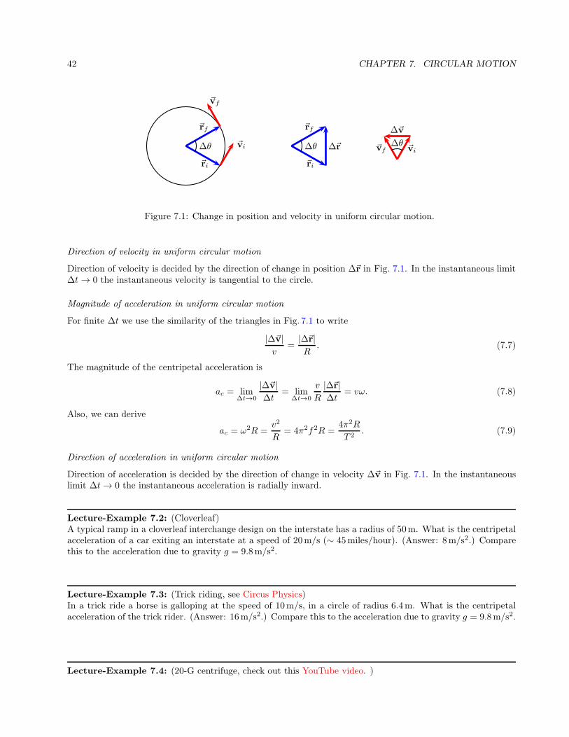
Figure 7.1: Change in position and velocity in uniform circular motion.

Direction of velocity in uniform circular motion

Direction of velocity is decided by the direction of change in position ∆~r in Fig. 7.1. In the instantaneous limit∆t → 0 the instantaneous velocity is tangential to the circle.

Magnitude of acceleration in uniform circular motion

For finite ∆t we use the similarity of the triangles in Fig. 7.1 to write

|∆~v|v

=|∆~r|R

. (7.7)

The magnitude of the centripetal acceleration is

ac = lim∆t→0

|∆~v|∆t

= lim∆t→0

v

R

|∆~r|∆t

= vω. (7.8)

Also, we can derive

ac = ω2R =v2

R= 4π2f2R =

4π2R

T 2. (7.9)

Direction of acceleration in uniform circular motion

Direction of acceleration is decided by the direction of change in velocity ∆~v in Fig. 7.1. In the instantaneouslimit ∆t → 0 the instantaneous acceleration is radially inward.

Lecture-Example 7.2: (Cloverleaf)A typical ramp in a cloverleaf interchange design on the interstate has a radius of 50m. What is the centripetalacceleration of a car exiting an interstate at a speed of 20m/s (∼ 45miles/hour). (Answer: 8m/s2.) Comparethis to the acceleration due to gravity g = 9.8m/s2.

Lecture-Example 7.3: (Trick riding, see Circus Physics)In a trick ride a horse is galloping at the speed of 10m/s, in a circle of radius 6.4m. What is the centripetalacceleration of the trick rider. (Answer: 16m/s2.) Compare this to the acceleration due to gravity g = 9.8m/s2.

Lecture-Example 7.4: (20-G centrifuge, check out this YouTube video. )

http://www.pbs.org/opb/circus/classroom/circus-physics/centripetal-acceleration

https://www.youtube.com/watch?v=FBJegTfF9Kg

7.2. UNIFORM CIRCULAR MOTION 43

The 20-G centrifuge of NASA has a radius of 29 feet (8.8m). What is the centripetal acceleration at theouter edge of the tube while the centrifuge is rotating at 0.50 rev/sec? (Answer: 9 g.) What is the centripetalacceleration at 0.70 rev/sec? (Answer: 17 g.) Note that such high acceleration causes damage to capillaries, seeTable 2.3.

Lecture-Example 7.5: (Gravitropism)The root tip and shoot tip of a plant have the ability to sense the direction of gravity, very much like smartphones. That is, root tips grow along the direction of gravity, and shoot tips grow against the direction ofgravity. (These are associated to statocytes.) Discuss the direction of growth of a plant when placed inside acentrifuge. What if the plant is in zero-gravity? Check out this YouTube video.

Lecture-Example 7.6: (Variation in g)The acceleration due to gravity is given by, (as we shall derive later in the course,)

g =GME

R2E

= 9.82 ms2, (7.10)

where ME = 5.97 × 1024 kg and RE = 6.37 × 106m are the mass and radius of the Earth respectively andG = 6.67× 10−11Nm2/kg2 is a fundamental constant. This relation does not take into account the rotation ofthe Earth about its axis and assumes that the Earth is a perfect sphere.

• The centripetal acceleration at a latitude φ on the Earth is given by

4π2

T 2E

RE = 0.034 cosφ, (7.11)

where TE = 24hours is the time period of the Earth’s rotation about its axis. It is directed towardsthe axis of rotation. The component of this acceleration toward the center of the Earth is obtained bymultiplying with another factor of cosφ. The contribution to g from the rotation of the Earth is largestat the equator and zero at the poles.

• The rotation of the Earth has led to its equatorial bulge, turning it into an oblate spheroid. That is,the radius of the Earth at the equator is about 20 km longer than at the poles. This in turn leads to aweaker g at the equator. The fractional change in gravity at a height h above a sphere is approximately,for h ≪ R, given by 2h/R. For h = 42km this leads to a contribution of 0.065m/s2.

• Contribution to g from rotation of the Earth is positive, and from the equatorial bulge is negative.Together, this leads to the variations in g on the surface of the Earth. Nevertheless, the variations in g arebetween 9.76m/s2 (in the Nevado summit in Peru) and 9.84m/s2 (in the Arctic sea), refer this article inGeophysical Research Letters (2013). The measurement of g is relevant for determining the elevation ofa geographic location on the Earth. An interesting fact is that even though Mount Everest is the highestelevation above sea level, it is the summit of Chimborazo in Equador that is farthest from the center ofthe Earth.

7.2 Uniform circular motion

A particle uniformly moving along a circular path is accelerating radially inward, given by

~a = −v2

Rr, (7.12)

https://www.youtube.com/watch?v=RxITZSEis4I

http://dx.doi.org/10.1002/grl.50838


where r is a unit vector pointing radially outward, R is the radius of the circle, and v is the magnitude of theuniform velocity. Newton’s law then implies that the sum of the total force acting on the system necessarilyhas to point radially inward.

Lecture-Example 7.7:A stuntman drives a car over the top of a hill, the cross section of which can be approximated by a circle ofradius R = 250m. What is the greatest speed at which he can drive without the car leaving the road at thetop of the hill?

m~g

~N


Lecture-Example 7.8:A turntable is rotating with a constant angular speed of 6.5 rad/s. You place a penny on the turntable.

• List the forces acting on the penny.

• Which force contributes to the centripetal acceleration of the penny?

• What is the farthest distance away from the axis of rotation of the turntable that you can place a pennysuch that the penny does not slide away? The coefficient of static friction between the penny and theturntable is 0.5.

Lecture-Example 7.9: (Motorcycle stunt)In the Globe of Death stunt motorcycle stunt riders ride motorcycles inside a mesh globe. In particular, theycan loop vertically. Consider a motorcycle going around a vertical circle of radius R, inside the globe, withuniform velocity. Determine the normal force and the force of friction acting on the motorcycle as a function ofangle θ described in Figure 7.3.

• Using Newton’s Laws we have the equations of motion, along the radial and tangential direction to thecircle, given by

N =mv2

R−mg cos θ, (7.13a)

Ff = mg sin θ. (7.13b)

• Investigate the magnitude and direction of the normal and force of friction as a function of angle θ. Inparticular, determine these forces for θ = 0,−90, 90. Verify that, while at θ = 90, the motorcyclecan not stay there without falling off unless the the centripetal acceleration is sufficiently high, that is,mv2/R ≥ mg.

7.3. BANKING OF ROADS 45

m~g

~N

θ m~g

~Ff

~Nm~g

~N

Figure 7.3: Forces acting on a mass while moving in a vertical circle inside a globe.

7.3 Banking of roads

Motorized cars are all around us, and we constantly encounter banked roads while driving on highways bendingalong a curve. A banked road is a road that is appropriately inclined, around a turn, to reduce the chances ofvehicles skidding while maneuvering the turn. Banked roads are more striking in the case of racetracks on whichthe race cars move many times faster than typical cars on a highway. Nevertheless, this ubiquitous presence ofbanked roads around us does not lessen the appreciation for this striking application of Newton’s laws.

Unbanked frictionless surface

A car can not drive in a circle on an unbanked frictionless surface, because there is no horizontal force availableto contribute to the (centripetal) acceleration due to circular motion.

Unbanked surface with friction

Consider a car moving with uniform speed along a circular path of radius R on a flat surface with coefficient ofstatic friction µs. Using Newton’s laws we have the equations of motion

Ff =mv2

R, (7.14a)

N = mg, (7.14b)

where Ff ≤ µsN . The maximum speed the car can achieve without sliding is given by

v2max = gR tan θs, (7.15)

where we used the definition of friction angle µs = tan θs.

Banked frictionless surface

Let the surface make an angle θ with respect to the horizontal. Even though there is no friction force due tothe geometry of the banking the normal force is able to provide the necessary centripetal acceleration. UsingNewton’s laws we have the equations of motion

N sin θ =mv2

R, (7.16a)

N cos θ = mg. (7.16b)

The speed of the car is given byv2 = gR tan θ. (7.17)

Thus, if the car speeds up it automatically gets farther away and vice versa.


Banked surface with friction

Let us now consider the case of a banked surface with friction. In this case both the normal force and the forceof friction are available to contribute to the centripetal acceleration. There now exists a particular speed v0that satisfies

v20 = gR tan θ, (7.18)

for which case the normal force alone completely provides the necessary centripetal force and balances the forceof gravity, see Figure 7.4. Thus, in this case, the frictional force is completely absent, as illustrated in Figure 7.4.The physical nature of the problem, in the sense governed by the direction of friction, switches sign at speedv0.

θmg

N

fs

vmin ≤ v < v0

θmg

N

v = v0

θmg

N

fs

v0 < v ≤ vmax

Figure 7.4: Forces acting on a car moving on a banked road. The car is moving into the page. The direction offriction is inward for v0 < v ≤ vmax, outward for vmin < v < v0, and zero for v = v0.

Let us begin by investigating what happens when the car deviates from this speed v0? If the speed of thecar is different from v0, the normal force alone cannot provide the necessary centripetal acceleration withoutsliding. Thus, as a response, the frictional force gets switched on. The frictional force responds to act (inwards)when the car moves faster than v0; this provides the additional force necessary to balance the centripetal force,see Figure 7.4. Similarly, the frictional force acts in the negative direction (outwards) when the car moves slower

than v0, see Figure 7.4. Let the frictional force be represented by ~Ff . Thus, for the case when the frictionalforce is acting inward, we have the equations of motion for the car given by,

N sin θ + Ff cos θ =mv2

R, (7.19a)

N cos θ − Ff sin θ = mg. (7.19b)

The equations of motion for the car when the frictional force is acting outward are given by Eqs. (7.19) bychanging the sign of Ff . Can the frictional force together with the normal force balance the centripetal forcefor all speeds? No. There exists an upper threshold to speed vmax beyond which the frictional force fails tobalance the centripetal force, and it causes the car to skid outward. Similarly, there exists a lower threshold tospeed vmin below which the car skids inward. To this end it is convenient to define

Ff ≤ µsN, µs = tan θs, (7.20)

where µs is the coefficient of static friction, and θs is a suitable reparametrization of the coefficient of staticfriction. The upper threshold for the speed is obtained by using the equality of Eq. (7.20) in Eq. (7.19) to yield

v2max = rg tan(θ + θs), (7.21)

where we used the definition in Eq. (7.20) and the trigonometric identity for the tangent of the sum of twoangles. Similarly, the lower threshold for the speed below which the car slides inward is given by

v2min = rg tan(θ − θs). (7.22)

7.3. BANKING OF ROADS 47

In summary, at any given point on the surface of the cone, to avoid skidding inward or outward in the radialdirection, the car has to move within speed limits described by

vmin ≤ v ≤ vmax. (7.23)

Chapter 8

Work and Energy

8.1 Scalar product

Scalar product of two vectors

~A = Ax i+Ay j+Az k, (8.1a)

~B = Bx i+By j+Bz k, (8.1b)

is given by~A · ~B = AB cos θ = AxBx +AyBy +AzBz, (8.2)

where θ is the angle between the two vectors. The scalar product is a measure of the component of one vectoralong another vector.

8.2 Work-energy theorem

Starting from Newton’s law~F1 + ~F2 + . . . = m~a, (8.3)

and integrating on both sides along the path of motion, we derive the work-energy theorem

W1 +W2 + . . . = ∆K, (8.4)

where Wi is the work done by the force ~Fi, (i = 1, 2, . . . ,) and ∆K is the change in kinetic energy.

Work done by a force

Work done by a force ~F on mass m while displacing it from an initial point ~ri to a final ~rf , along a path P , isgiven by

W =∑

P

∆~r · ~F. (8.5)

Work done is measured in the units of energy, Joule=Newton ·meter.

Kinetic energy

The energy associated with the state of motion, the kinetic energy, is

K =1

2mv2, (8.6)

49

50 CHAPTER 8. WORK AND ENERGY

where v is the magnitude of the velocity of mass m.

Lecture-Example 8.1: (Area under the force-position graph.)Consider the motion of a mass m under the action of a force

F = −kx, (8.7)

where k is a constant. Show that the work done by the force is equal to the area under the force-position graph.

x

F

xi xf

Figure 8.1: A Force-position graph.

• The work done by the force is

W =

f∑

i

(−kx)∆x = −1

2k(x2

f − x2i ). (8.8)

• Show that the area under the force-position graph is the sum of the area of a triangle and a rectangle,

W = −1

2k(xf − xi)

2 − kxi(xf − xi). (8.9)

Lecture-Example 8.2:Consider a mass m = 25kg being pulled by a force Fpull = 80.0N, exerted horizontally, such that the massmoves, on a horizontal surface with coefficient of kinetic friction µk = 0.30. Assume that the mass starts fromrest. We would like to determine the final velocity vf after the mass has moved a horizontal distance d = 10.0m.

• We identify four forces acting on the mass and write Newton’s law for the configuration as

m~g+ ~N+ ~Fpull + ~Ff = m~a. (8.10)

• Work done by the individual force are

Wpull = Fpulld cos 0 = Fpulld = 800 J, (8.11a)

Wg = mgd cos 90 = 0 J, (8.11b)

WN = Nd cos 90 = 0 J, (8.11c)

Wf = Ffd cos 180 = −Ffd = −µkNd = −µkmgd = −735 J, (8.11d)

where we used Ff = µkN , and then used Newton’s law in the vertical y-direction to learn that N = mg.

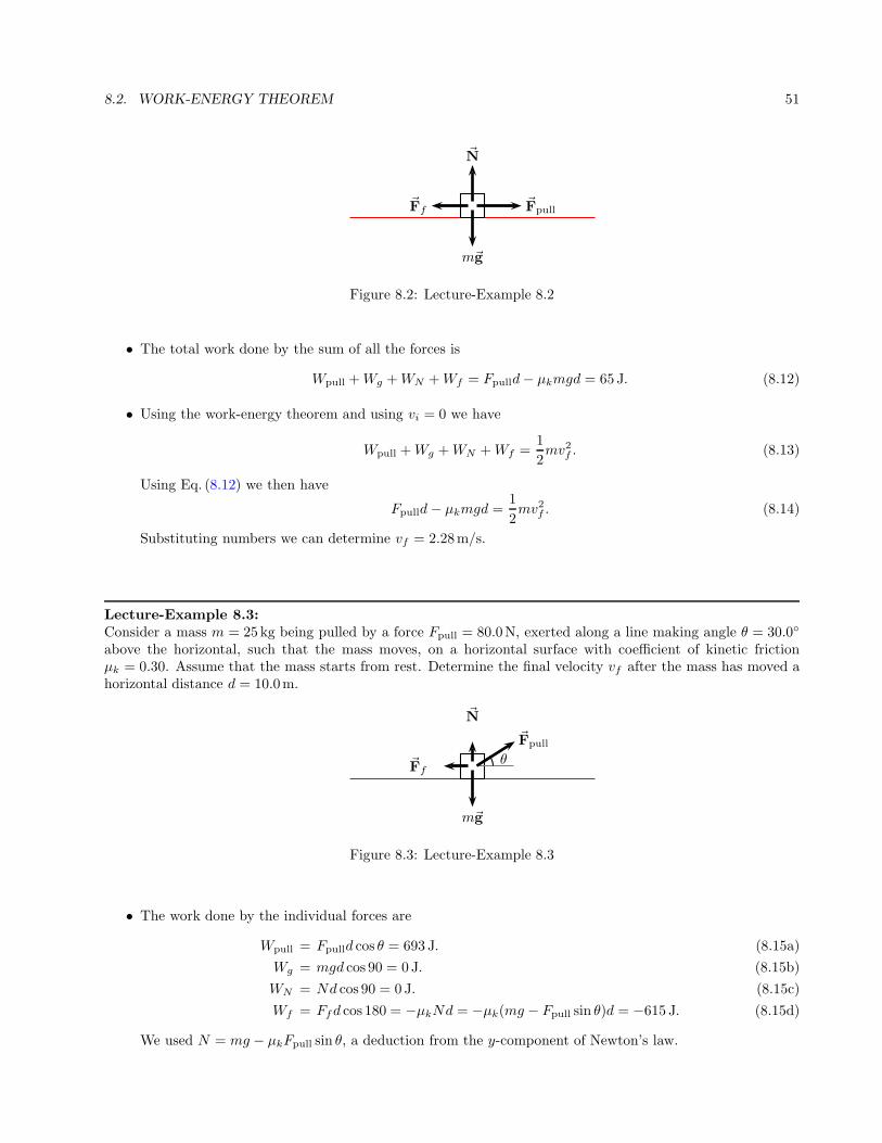
8.2. WORK-ENERGY THEOREM 51

~Fpull~Ff

~N

m~g


• The total work done by the sum of all the forces is

Wpull +Wg +WN +Wf = Fpulld− µkmgd = 65 J. (8.12)

• Using the work-energy theorem and using vi = 0 we have

Wpull +Wg +WN +Wf =1

2mv2f . (8.13)

Using Eq. (8.12) we then have

Fpulld− µkmgd =1

2mv2f . (8.14)

Substituting numbers we can determine vf = 2.28m/s.

Lecture-Example 8.3:Consider a mass m = 25kg being pulled by a force Fpull = 80.0N, exerted along a line making angle θ = 30.0

above the horizontal, such that the mass moves, on a horizontal surface with coefficient of kinetic frictionµk = 0.30. Assume that the mass starts from rest. Determine the final velocity vf after the mass has moved ahorizontal distance d = 10.0m.

~Fpull

θ~Ff

~N

m~g


• The work done by the individual forces are

Wpull = Fpulld cos θ = 693 J. (8.15a)

Wg = mgd cos 90 = 0 J. (8.15b)

WN = Nd cos 90 = 0 J. (8.15c)

Wf = Ffd cos 180 = −µkNd = −µk(mg − Fpull sin θ)d = −615 J. (8.15d)

We used N = mg − µkFpull sin θ, a deduction from the y-component of Newton’s law.


• Using the work energy theorem we obtain

Kf = Fpulld(cos θ + µk sin θ)− µkmgd, (8.16)

which leads to vf = 2.50m/s.

Lecture-Example 8.4:A mass m = 25kg slides down an inclined plane with angle θ = 30.0. Assume coefficient of kinetic frictionµk = 0.30. Assume that the mass starts from rest. Determine the final velocity vf after the mass has moved adistance d = 10.0m along the incline.

• Determine the work done by the three individual forces.

• Using the work-energy theorem deduce

Kf = mgd sin θ − µkmgd cos θ. (8.17)

This leads to vf = 6.86m/s.

• Observe that the final velocity is independent of mass m.

8.3 Conservative forces and potential energy

The work done by a conservative force is independent of the path taken by the mass. Thus, the work doneby a conservative force is completely determined by the initial and final position of the mass. That is, thework done by the force is conveniently defined as the negative change in potential energy U associated with theconservative force,

W =

f∑

i

∆~r · ~F = −∆U. (8.18)

The work-energy theorem, with emphasis on this distinction, is

(W nc1 +W nc

2 + . . .) + (W c1 +W c

2 + . . .) = ∆K, (8.19)

where ‘nc’ in superscript stands for non-conservative force and ‘c’ in superscript stands for conservative force.It is then expressed in the form

(W nc1 +W nc

2 + . . .) = ∆K + (∆U1 +∆U2 + . . .). (8.20)

Thus, if there are no non-conservative forces acting on the system, the change in energy of the system isindependent of the path and is completely determined by the initial and final positions.

Gravitational potential energy

The force of gravity is a conservative force. The work done by the gravitational force is completely determinedby the change in height of the mass m,

Wg = −mg∆y = −∆Ug, (8.21)

where ∆y = yf − yi. It depends only on the initial and final heights. Thus, it is conveniently expressed in termsof the gravitational potential energy function

Ug = mgy. (8.22)


8.3. CONSERVATIVE FORCES AND POTENTIAL ENERGY 53

• Determine the work done by force of gravity in the following processes.

1. A person lifts am = 3.0 kg block a vertical distance h = 10.0m and then carries the block horizontallya distance x = 50.0m.

2. A person carries the block horizontally a distance x = 50.0m and then lifts it a vertical distanceh = 10.0m

3. A person carries the block along the diagonal line.

• Observe that the work done by the force of gravity is independent of the path. Observe that the workdone by force of gravity is zero along a closed path. Observe that the force of gravity does not do anywork while moving horizontally. An arbitrary path can be broken into vertical and horizontal sections,which corresponds to path independence.

Lecture-Example 8.6:A mass of m = 25.0kg slides down a frictionless incline that makes an angle of θ = 30.0 with the horizontal.Assume that the mass starts from rest. The two forces acting on the mass during the slide are the normal forceand the force of gravity. The mass slides d = 10.0m along the incline.

• Work-energy theorem statesWN +Wg = ∆K. (8.23)

The work done by the normal force is zero,WN = 0. (8.24)

The work done by the force of gravity on the mass is

Wg = mgd cos(90− θ) = mgd sin θ = 1225 J. (8.25)

• The change in gravitational potential energy is

∆Ug = −Wg = −1225 J. (8.26)

Since WN = 0, the change in kinetic energy of the mass is equal to the work done by the force of gravity,

∆K = Wg = 1225 J. (8.27)

The velocity of the mass at the end of the slide is then determined to be 9.90m/s.

Lecture-Example 8.7: (Roller coaster)A roller coaster of mass m = 500.0kg moves on the curve described in Figure 8.4. Assume frictionless surface.It starts from rest, vA = 0m/s at point A height hA = 40.0m.

• Work-energy theorem statesWN +Wg = ∆K. (8.28)

Show that the work done by the normal force is zero, WN = 0. Thus, conclude

∆K +∆Ug = 0, or Ki + Ui = Kf + Uf . (8.29)

• Determine the velocity of the mass at points A to G, given hB = 20.0m, hC = 30.0m, hD = 10.0m,hE = 20.0m, hF = 0m, hG = 45.0m. (Answer: See Table 8.1.) Note that the above results areindependent of the mass.


O

A

B

C

D

E

F

G

Figure 8.4: Lecture-Example 8.7.

point h v U K U+KA 40.0m 0m/s 196kJ 0 kJ 196kJB 20.0m 19.8m/s 98 kJ 98 kJ 196kJC 30.0m 14.0m/s 147kJ 49 kJ 196kJD 10.0m 24.3m/s 49 kJ 147kJ 196kJE 20.0m 19.8m/s 98 kJ 98 kJ 196kJF 0m 28m/s 0 kJ 196kJ 196kJG 45.0m - - - -

Table 8.1: Lecture-Example 8.7.

• The roller coaster will not reach the point G because it does not have sufficient total energy.

Lecture-Example 8.8:Figure 8.5 shows a pendulum of length L = 3.0m and mass m = 5.0 kg. It starts from rest at angle θ = 30.0.Determine the velocity of the mass when θ = 0.

θ

L

h

Figure 8.5: Lecture-Example 8.8.

• Work-energy theorem statesWT +Wg = ∆K. (8.30)

Show that the work done by the tension in the rod is zero,

WT = 0. (8.31)


Using h = L− L cos θ, we have

mghi +Ki = mghf +Kf . (8.32)

• How much work does its weight do on the ball?

• What is the change in the gravitational potential energy of the ball Earth system?

• What is the kinetic energy of the ball at its lowest point?

• What is the velocity of the ball at its lowest point?

• If mass m were doubled, would the velocity of the ball at its lowest point increase, decrease, or remainsame?

Elastic potential energy of a spring

Elastic materials, for example a spring, when stretched exhibit a restoring force in the opposite direction of thestretch. This is stated as Hooke’s law,

F = −kx, (8.33)

where for the case of springs k is a material dependent quantity called the spring constant. The work done byan elastic force is

Ws =

f∑

i

(−kx)∆x = −(

1

2kx2

f − 1

2kx2

i

)

. (8.34)

Thus, using W = −∆U , we read out the elastic potential energy function

Us =1

2kx2. (8.35)

Lecture-Example 8.9: (Spring constant)A mass of 5.0 kg is hung using a spring. At equilibrium the spring is stretched 5.0 cm. Determine the springconstant.

• At equilibrium the force of gravity balances the elastic restoring force,

kx = mg. (8.36)

(Answer: k = 980 ∼ 103N/m.) This could be the spring constant of a spring in a simple weighing scale.

• A car weighing 2000kg is held by four shock absorbers. Thus, each spring gets a load of 500kg. Atequilibrium if the spring is stretched by 5.0 cm, determine the spring constant of a typical shock absorber.(Answer: k ∼ 105N/m.)

Lecture-Example 8.10:A mass m slides down a frictionless incline, starting from rest at point A. After sliding down a distance L(along the incline) it hits a spring of spring constant k at point B. The mass is brought to rest at point C whenthe spring is compressed by length x. See Figure 8.6.


CB

A

L

x


• Using work-energy theorem we haveWN +Wg +Ws = ∆K. (8.37)

Show that the work done by the normal force is zero, WN = 0. Thus, derive

KA + UgA + Us

A = KB + UgB + Us

B = KC + UgC + Us

C . (8.38)

• Show that the velocity of the mass at point B is given by

v2B = 2gL sin θ. (8.39)

• Show that the maximum compression x in the spring at point C is given by the quadratic equation,

x2 − 2x0x− 2x0L = 0, (8.40)

in terms of the compression x0 in the spring at equilibrium, given by

x0 =mg

ksin θ. (8.41)

Thus, we havex = x0 ±

√

x0(x0 + 2L). (8.42)

For x0 ≪ 2L, show that the solution has the limiting form

x ∼√

2x0L. (8.43)

For 2L ≪ x0, show that the solution has the limiting form x ∼ L.

Lecture-Example 8.11:A mass m = 20.0 kg slides down a frictionless incline, starting from rest at point A at height h = 1.0m. Aftersliding down the incline it moves horizontally on a frictionless surface before coming to rest by compressing aspring of spring constant k = 2.0× 104N/m by a length x. See Figure 8.7.

• Using work-energy theorem we haveWN +Wg +Ws = ∆K. (8.44)

Show that the work done by the normal force is zero, WN = 0. Thus, derive

KA + UgA + Us

A = KB + UgB + Us

B = KC + UgC + Us

C . (8.45)

• Determine the velocity of the mass at point B. (Answer: 4.4m/s.)

• Determine the maximum compression x in the spring. (Answer: 14 cm.)


θCB

A

hx


Chapter 9

Collisions: Conservation of linearmomentum

9.1 Momentum

Using the definition of momentum,

~p = m~v, (9.1)

Newton’s laws can be expressed in the form

~J1 + ~J2 + . . . = ∆~p, (9.2)

where~Ji =

∑

~Fi∆t (9.3)

is the impulse due to force ~Fi.

Lecture-Example 9.1: When a ball of mass m1 = 1.00kg is falling (on Earth of mass m2 = 5.97× 1024 kg)what are the individual accelerations of the ball and Earth?

Lecture-Example 9.2: A student of mass m = 60.0 kg jumps off a table at height h = 1.00m. While hittingthe floor he bends his knees such that the time of contact is 100.0ms. What is the force exerted by the floor onyou? If the student does not bend his knees the time of contact is 10.0ms. What is the new force exerted bythe floor now? (Answer: 2660N versus 26600N.)

Lecture-Example 9.3: A drop of rain and a pellet of hail, of the same mass m = 1.00 g, hits the roof of acar with the same speed v = 5.00m/s. Rain drop being liquid stays in contact with the roof for 100.0ms, whilehail being solid rebounds (assume with same speed v = 5.00m/s) and thus stays in contact for a mere 1.00ms.Calculate the force exerted by each on the roof of the car. (The numbers quoted here are based on reasonableguesses, and could be off by an order of magnitude.)

59

60 CHAPTER 9. COLLISIONS: CONSERVATION OF LINEAR MOMENTUM

9.2 Conservation of linear momentum

If the net external force on a system is zero the change in momentum is zero, or the momentum is conserved.In a collision involving two masses we can write

~Fext1 + ~C12 =

∆~p1

∆t, (9.4)

~Fext2 + ~C21 =

∆~p2

∆t, (9.5)

where ~C12 and ~C21 are contact forces, which are action-reaction pairs that are equal and opposite in directions.If the external forces add up to to zero there is no change in momentum and we have the conservation of linearmomentum

~p1i + ~p2i = ~p1f + ~p2f . (9.6)

9.2.1 Inelastic collisions

Using conservation of linear momentum we have

m1~v1i +m2~v2i = m1~v1f +m2~v2f . (9.7)

The particular case when the masses entangle together before or after the collision is called a completely inelasticcollision.

Lecture-Example 9.4:A shooter of mass m2 = 90.0 kg shoots a bullet of mass m1 = 3.00 g horizontally, standing on a frictionlesssurface at rest. If the muzzle velocity of the bullet is v1f = 600.0m/s, what is the recoil speed of the shooter?(Answer: v2f = −2.00 cm/s.)

Lecture-Example 9.5:A shooter of mass m2 = 90.0kg shoots a bullet of mass m1 = 3.00 g in a direction θ = 60.0 with respect tothe horizontal, standing on a frictionless surface at rest. If the muzzle velocity of the bullet is v1f = 600.0m/s,what is the recoil speed of the shooter? (Answer: v2f = −1.00 cm/s.)

Lecture-Example 9.6: (Ballistic pendulum)A bullet with mass m1 = 3.00 g is fired into a wooden block of mass m2 = 1.00kg, that hangs like a pendulum.The bullet is embedded in the block (complete inelastic collision). The block (with the bullet embedded in it)goes h = 30.0 cm high after collision. Calculate the speed of the bullet before it hit the block.

Lecture-Example 9.7: (Collision of automobiles at an intersection.)A car of mass m1 = 2000.0kg is moving at speed v1i = 20.0m/s towards East. A truck of mass m2 = 5000.0kgis moving at speed v2i = 10.0m/s towards North. They collide at an intersection and get entangled (completeinelastic collision). What is the magnitude and direction of the final velocity of the entangled automobiles?

• Repeat the calculation for a semi-truck (ten times heavier) moving at the same speed.

9.2. CONSERVATION OF LINEAR MOMENTUM 61

9.2.2 Elastic collisions in 1-D

In an elastic collision, in addition to momentum being conserved, the kinetic energy is also conserved. Thisrequires no loss of energy in the form of sound and heat. Conservation of kinetic energy leads to

1

2m1v

21i +

1

2m2v

22i =

1

2m1v

21f +

1

2m2v

22f . (9.8)

In conjunction with the conservation of momentum,

m1v1i +m2v2i = m1v1f +m2v2f , (9.9)

this leads to the corollary

v1i + v1f = v2i + v2f . (9.10)

Together we can solve for the final velocities:

v1f =

(

m1 −m2

m1 +m2

)

v1i +

(

2m2

m1 +m2

)

v2i, (9.11a)

v2f =

(

2m1

m1 +m2

)

v1i +

(

m2 −m1

m1 +m2

)

v2i. (9.11b)

Consider the following cases:

1. m1 = m2: Implies swapping of velocities!

2. v2i = 0:

3. v2i = 0, m1 ≪ m2:

4. v2i = 0, m1 ≫ m2:

Lecture-Example 9.8: A mass m1 = 1.00kg moving with a speed v1i = +10.0m/s (elastically) collides withanother mass m2 = 1.00 kg initially at rest. Describe the motion after collision. (Answer: v1f = 0m/s andv2f = −v1i = +10.0m/s.)

Lecture-Example 9.9: A mass m1 = 1.00kg moving with a speed v1i = +10.0m/s (elastically) collides withanother mass m2 = 100.0kg initially at rest. Describe the motion after collision. (Answer: v1f = −9.80m/sand v2f = +0.198m/s.)

Lecture-Example 9.10: A mass m1 = 100kg moving with a speed v1i = +10m/s (elastically) collides withanother mass m2 = 1kg initially at rest. Describe the motion after collision. (Answer: v1f = +9.80m/s andv2f = +19.8m/s.)

Lecture-Example 9.11: (Rebounce of tennis ball on basketball.)A tennis ball of mass m1 = 60.0 g is dropped with a basketball of mass m2 = 0.600kg from a height of h = 1m.How high does the tennis ball return back?

62 CHAPTER 9. COLLISIONS: CONSERVATION OF LINEAR MOMENTUM

Lecture-Example 9.12: An electron collides elastically with a stationary hydrogen atom. The mass of thehydrogen atom is 1837 times that of the electron. Assume that all motion, before and after the collision, occursalong the same straight line. What is the ratio of the kinetic energy of the hydrogen atom after the collision tothat of the electron before the collision?

Using Eqs. (9.11) for elastic collisions in 1-D, with m2 = 1837m1 and v2i = 0, obtain

v2fv1i

=2

1838. (9.12)

Then, we have the ratio

K2f

K1i

=m2

m1

(

v2fv1i

)2

= 1837

(

2

1838

)2

∼ 1

459.8. (9.13)

9.3 Center of mass

The center of mass of a distribution of mass (in one dimension) is defined as

xcm =

N∑

i=1

mixi

N∑

i=1

mi

. (9.14)

In the language of statistics, center of mass is the first moment of mass. The total mass itself is the zerothmoment of mass. The term weighted average is based on this concept. In three dimensions the center of massof a distribution of mass is defined as

~rcm =

N∑

i=1

mi~ri

N∑

i=1

mi

. (9.15)

Lecture-Example 9.13: (Meter stick)A uniform meter stick has a mass m1 = 10.0 kg placed at 100.0 cm mark and another mass m2 = 20.0 kgplaced at 20.0 cm mark. Determine the center of mass of the stick and the two masses together. (Answer:xcm = 46.7 cm.)

Lecture-Example 9.14: (Earth-Moon)Determine the center of mass of the Earth-Moon system. In particular, determine if the center of mass ofthe Earth-Moon system is inside or outside the Earth. Given the masses MEarth = 5.97 × 1024 kg, MMoon =7.35 × 1022 kg, the radiuses REarth = 6.37 × 106m, RMoon = 1.74 × 106m, and the distance between them isr = 384 × 106m. (Answer: 4.67 × 106m from the center of Earth on the line passing through the centers ofEarth and Moon.)

Lecture-Example 9.15:Three masses are placed on a plane such that the coordinates of the masses are,m1 = 1.0 kg at (1, 0), m2 = 2.0 kgat (2, 0), and m3 = 3.0 kg at (0, 3). Determine the coordinates of the center of the mass of the three masses.(Answer: (5

6, 32).)

Chapter 10

Rotational motion

10.1 Rotational kinematics

A rigid object will be defined as an object with the constarint that the relative distances of any two pointsinside the body does not vary with time. We will confine our attention to rotational motion of rigid bodiesabout a fixed axis. Thus, the motion of a particle is confined to a plane perpendicular to the axis.

Since the distance of a point from the axis remains fixed for a rigid body, we can specify the motion of thispoint with respect to the axis by specifying the angle it is rotated. The infinitismal angular displacement isdefined as the vector ∆θ whose direction specifies the axis of rotation and the magnitude specifies the amountof rotation about the axis. The change in position of a point due to this rotation for the case of rigid rotationis simply is given by

∆s = r∆θ. (10.1)

We immediately have the relation, (dividing by ∆t,)

v = ω r, (10.2)

in terms of the angular velocity

ω =∆θ

∆t. (10.3)

The angular acceleration is defined using the relation

α =∆ω

∆t. (10.4)

The linear acceleration, the rate of change of linear velocity, for the case of rigid rotation, thus has a radial anda tangential component corresponding to the tangential and radial accelerations

aT = α r and ar = −ω2r, (10.5)

respectively.

Rotation motion with constant angular acceleration

For the case of rotation motion with constant angular acceleration the angular velocity and the angular accel-eration are given by

∆θ

∆t=

ωf + ωi

2, (10.6a)

α =ωf − ωi

∆t. (10.6b)

63

64 CHAPTER 10. ROTATIONAL MOTION

Eqs. (10.6a) and (10.6b) are two independent equations involving five independent variables: ∆t,∆θ, ωi, ωf , α.We can further deduce,

∆θ = ωi∆t+1

2α∆t2, (10.6c)

∆θ = ωf∆t− 1

2α∆t2, (10.6d)

ω2f = ω2

i + 2α∆θ, (10.6e)

obtained by subtracting, adding, and multiplying, Eqs. (10.6a) and (10.6b), respectively.

Lecture-Example 10.1:Starting from rest a wheel rotates with uniform angular acceleration 3.0 rad/s2. Determine the angular velocityof the wheel after 3.0 s.

10.2 Torque

The ability of a force to contribute to rotational motion, about an axis, is measured by torque

τ = rF⊥, (10.7)

where F⊥ is the component of force ~F in the tangential direction.

Lecture-Example 10.2:A force of 10.0N is exerted on a door in a direction perpendicular to the plane of the door at a distance of40.0 cm from the hinge. Determine the torque exerted by the force. (Answer: 4.00Nm.)

10.3 Moment of inertia

For a particle rotating ‘rigidly’ about an axis, the tendency to be in the state of rotational rest or constantangular velocity, the rotational inertia, is given by the moment of inertia

I = mr2, (10.8)

where r is the perpendicular distance of the mass m to the axis. The moment of inertia of a distribution ofmass is given by

I =N∑

i=1

mir2i . (10.9)

In the language of statistics, moment of inertia is the second moment of mass.

Lecture-Example 10.3: (Rotational inertia)A massless rod is hinged so that it can rotate about one of its ends. Masses m1 = 1.0 kg and m2 = 20.0 kgare attached to the rod at r1 = 1.0m and r2 = 5.0 cm respectively. Determine the moment of inertia of theconfiguration. (Answer: 1.1 kg·m2.)

• Repeat the calculation for r2 = 0.5m. (Answer: 6.0 kg·m2.)

10.4. ROTATIONAL DYNAMICS 65

Lecture-Example 10.4: (Uniform rod)Determine the moment of inertia of an infinitely thin rod of massM and length L, when the axis is perpendicularto the rod and passing through the center of the rod. (Answer: I = ML2/12.) Repeat for the case when theaxis is perpendicular to the rod and passing through on of the ends of the rod. (Answer: I = ML2/3.)

Lecture-Example 10.5: (Comparing moment of inertia)Show that

Isolid sphere

about diameter

< Isolid cylinder

about axis

< Ispherical shell

about diameter

< Icylindrical shell

about axis

. (10.10)

10.4 Rotational dynamics

For the case when the moment of of inertia I of a body does not change in time, the rotational dynamics isdescribed by the equation

~τ1 + ~τ2 + . . . = I ~α. (10.11)

Lecture-Example 10.6:A uniform solid cylinder of radius R and mass M is free to rotate about its symmetry axis. The cylinder actslike a pulley. A string wound around the cylinder is connected to a mass m, which falls under gravity. SeeFig. 10.1. What is the angular acceleration α of the cylinder?

m


• Using Newton’s law, for the mass m, show that

mg − T = ma, (10.12)

where T is the tension in the string. Using the Newton’s law for torque, for the mass M , deduce therelation

T =1

2MRα. (10.13)

Presuming the string does not stretch and rolls the cylinder perfectly we also have the constraint

a = αR. (10.14)

• Determine the acceleration a of the mass m to be

a =m

(

m+ M2

)g. (10.15)

Determine the angular acceleration α of the cylinder, and the tension T in the string.


10.5 Rotational work-energy theorem

The rotational work-energy theorem states

W1 +W2 + . . . = Krot, (10.16)

where the work done by the torque τi, while the particle is moving along path P , is given by

Wi =∑

P

τi∆θ (10.17)

and the rotational kinetic energy is given by

Krot =1

2Iω2. (10.18)

Lecture-Example 10.7:A solid sphere and a spherical shell, both of same mass M and same radius R, start from rest at a height h onan incline.

h


• Using the translational work-energy theorem show that

mgh− Ffd =1

2Mv2, (10.19)

where Ff is the force of friction and d is the distance along the incline. Using rotational work-energytheorem show that

FfRθ =1

2Iω2, (10.20)

where θ is the angular displacement corresponding to the distance d. For rolling without slipping or slidingargue that

d = Rθ and v = ωR. (10.21)

Verify that, for rolling motion, there is no work done by the force of friction. That is, for rolling motion,the translational work done by the force of friction exactly cancels the rotational work done by the forceof friction. Thus, deduce the relation

mgh =1

2Mv2 +

1

2Iω2. (10.22)

Determine the velocity of the solid sphere and the spherical shell to be

v =

√

2gh

1 + p, (10.23)

where we defined I = pMR2.

10.6. DIRECTION OF FRICTION ON WHEELS 67

• Using translational Newton’s law show that

mg sin θ − Ff = ma, (10.24)

and using rotational Newton’s law show that

FfR = Iα. (10.25)

Thus, deduce the relation

a =g sin θ

1 + p. (10.26)

• Model a raw egg as a spherical shell and a boiled egg as a solid sphere, and deduce which of them will rolldown the incline faster.

10.6 Direction of friction on wheels

Consider an illustrative example consisting of a simple two-wheeler. It consists of two wheels connected by arod. The front wheel is driven by a torque provided by an engine, and the rear wheel is pulled forward bythe rod. Thus, the front wheel is driven by a torque, and the rear wheel is driven by a force. Let us assumeperfect rolling, with no slipping or sliding. Let the front wheel have radius R1, mass m1, and moment of inertiaI1 = p1m1R

21, and let the rear wheel have radius R2, mass m2, and moment of inertia I2 = p2m2R

22,

Accelerating forward while moving forward

Friction acts in the forward direction on the front wheel, and in the backward direction on the rear wheel. Notethat Fpull is the same on both the tires because of Newton’s third law.

F1f

FpullFpull

F2f

τe

Figure 10.3: A simple two-wheeler accelerating forward.

τe −R1F1f = I1α1 (Torque equation for front wheel), (10.27a)

F1f − Fpull = m1a1 (Force equation for front wheel), (10.27b)

R2F2f = I2α2 (Torque equation for rear wheel), (10.27c)

Fpull − F2f = m2a2 (Force equation for rear wheel). (10.27d)

For rolling motion, we have the constraints,

a1 = α1R1 and a1 = α1R1, (10.28)

and the rigidity of the two-wheel configuration further requires the constraint

a1 = a2 = a. (10.29)

Thus, we can derive the acceleration of the two-wheeler using

a =τe

R1

[

(1 + p1)m1 + (1 + p2)m2

] . (10.30)


In terms of the acceleration of the system we can determine all other forces. For the particular caseR1 = R2 = R,m1 = m2 = m, and p1 = p2 = 1/2,

ma = 2F2f =2

3Fpull =

2

5F1f =

1

3

τeR. (10.31)

Constant speed

What happens if the engine was switched off? Using Eq. (10.31) we learn that this requires the accelerationa to be zero, which immediately implies that all the forces are zero in this case. This is unphysical, and is aconsequence of the extreme constraint imposed by perfect rolling.

To understand this, consider a single wheel rolling forward under the influence of friction alone. If thefriction is assumed to be acting in the forward direction it will lead to translational acceleration, with angulardecceleration of the wheel, which is possible simultaneaously only when imperfect rolling is allowed, or whenfrictional force is zero.

Accelerating backward (deccelerating) while moving forward

Next, let a torque τb be applied, using brakes, on the front wheel. Friction acts in the backward direction onthe front wheel, and in the forward direction on the rear wheel.

F1f

FpullFpull

F2f

τb

Figure 10.4: A simple two-wheeler deccelerating.

−τb +R1F1f = −I1α1 (Torque equation for front wheel), (10.32a)

−F1f + Fpull = −m1a1 (Force equation for front wheel), (10.32b)

−R2F2f = −I2α2 (Torque equation for rear wheel), (10.32c)

−Fpull + F2f = −m2a2 (Force equation for rear wheel). (10.32d)

Thus, we can derive the acceleration of the two-wheeler using

a =τb

R1

[

(1 + p1)m1 + (1 + p2)m2

] . (10.33)

This leads to the same magnitudes for the forces as in the case of forward acceleration.

Lecture-Example 10.8: (Comments)The key observation is that the friction on the front wheel opposes the torque and the friction on the rear wheelopposes the force. In more complicated systems a wheel is acted on by torques and forces simultaneously, andin such situations the friction opposes either the torque or the force at a given moment in time.

• Which tires (front or rear) wears more due to friction?

• For perfect rolling verify that the total work done by the force of friction is zero.

• Derive the above expressions for the case when the system is accelerating backward by applying brakes inthe rear wheel alone.

10.7. ANGULAR MOMENTUM 69

10.7 Angular momentum

Using the definition of angular momentum,L = Iω, (10.34)

the torque equation can be expressed in the form in terms of impulse due to individual torques. If the externaltorques add up to to zero there is no change in angular momentum and we have the conservation of angularmomentum

L1i + L2i = L1f + L2f . (10.35)

Lecture-Example 10.9: A merry-go-round, in the shape of a disc, is free to rotate (without friction) about itssymmetry axis. (It has mass M = 100.0,kg, radius R = 2.00m, and moment of inertia I = 1

2MR2.) A kid (mass

m = 25.0kg) walks from the outer edge of the disc to the center. If the angular speed of the merry-go-roundwas ωi = 0.30 rev/s when the kid was at the outer edge, what is the angular speed of the merry-go-round whenthe kid is at the center?

• Use conservation of angular momentum,

Ldisci + Lkid

i = Ldiscf + Lkid

f , (10.36)

to derive

ωf =

(

1 +2m

M

)

ωi. (10.37)

Part II

Electricity and Magnetism

401

Chapter 18

Electric force and electric Field

18.1 Electric charge

Like mass is a fundamental property of an object, electric charge is another fundamental property of an objector a particle. Unlike mass, which is always non-negative, charge can be positive or negative. Charge is measuredin units of Coulomb.

1. Electric charge is always conserved.

2. Electric charge is quantized. That is, it always comes in integer multiples of a fundamental charge

e ∼ 1.60× 10−19C. (18.1)

It is instructive to compare the electric charge and mass of the three particles that constitutes all atoms.

Particle Charge MassElectron −e ∼ 9.10× 10−31 kgProton +e ∼ 1.672× 10−27 kgNeutron 0 ∼ 1.674× 10−27 kg

3. All macroscopic objects get their charge from the electrons and protons that constitute them. Chargesare not always free to move inside an object. We will often imagine two extremes: A perfect conductorin which the charges are completely free to move, and a perfect insulator in which the charges are static.Metals (like gold and copper) are close to perfect conductors, and wood and rubber are close to perfectinsulators. Vacuum is the perfect insulator.

To get an an insight of the amount of charge contained in a Coulomb of charge we list a few typical chargeswe encounter in Table 18.1.

Lecture-Example 18.1:Determine the number of electrons in one gram of electron. Then calculate the total charge of one gram ofelectron.

• One gram of electron has about 1030 electrons, and a total charge of about 1011C, an enormous amountof charge.

• One gram of proton has about 1027 protons, and a total charge of about 108C.

403

404 CHAPTER 18. ELECTRIC FORCE AND ELECTRIC FIELD

10−19C charge on an electron10−15C charge on a typical dust particle10−6C this much isolated charge when confined to a region of 10 cm (a

typical hand) causes breakdown of air (static electricity).101C this much isolated charge when confined to a region of 1000m (a

typical thundercloud) causes breakdown of air (lightning).103C total charge generated in an alkaline battery. This is not isolated

charge, so does not breakdown air.106C this much isolated charge when confined to a region of 1m has

been predicted to breakdown vacuum.

Table 18.1: Orders of magnitude (charge)

18.2 Coulomb’s law

The electrostatic force between two objects with charges q1 and q2, separated by distance r, is

~F = keq1q2r2

r, (18.2)

where r encodes the direction content of the force. The constant of proportionality is ke ∼ 8.99× 109Nm2/C2,which is often expressed in terms the permittivity of vacuum,

ε0 ∼ 8.85× 10−12 C2

Nm2, using ke =

1

4πε0. (18.3)

Lecture-Example 18.2: (Static electricity)Consider a neutral balloon of mass m = 10.0 g blown up so that it is a sphere of radius R = 10.0 cm. I can rubit on me so that a certain amount of charge Q is transferred from the balloon to my hand, so that the balloonand me have unlike charges on us. The balloon balances under gravity! Determine the charge Q.

• The gravitation force on the balloon is nulled by the electrostatic force,

mg =kQ2

R2. (18.4)

This leads to Q = 3.30× 10−7C.

Lecture-Example 18.3: A hydrogen atom consists of an electron orbiting a proton. The radius is about5.3× 10−11m.

• Find the electrostatic force between electron and proton.

Felectric =ke2

R2∼ 10−8N. (18.5)

• Find the gravitational force between electron and proton.

Fgravity =Gmemp

R2∼ 10−47N. (18.6)

18.2. COULOMB’S LAW 405

• Find the ratio of the electrostatic force to gravitational force. (This is independent of the radius.)

Felectric

Fgravity

=ke2

Gmemp

∼ 1040. (18.7)

Lecture-Example 18.4: Can we detach the Moon?If charges of same sign are placed on Earth and Moon it could be possible to negate the gravitational forcebetween them. (mEarth ∼ 6×1024 kg, mMoon ∼ 7×1022 kg.) (You do not need the knowledge of the Earth-Moondistance for this calculation, R ∼ 4× 108m.)

• Equating the gravitational force to the electrostatic force we have

GmEmmoon

R2=

kq2

R2. (18.8)

• Thus, the charge needed to release the Moon is q = 1012C, which is about 1 kg of electrons. This is astupendous amount of charge, which when confined to the volume of Earth will breakdown the atmosphere,though not breakdown vacuum!

Lecture-Example 18.5: Charges q1 = +3.0µC and q2 = −1.0µC are placed a distance x0 = 10.0 cm apart.Presume the two charges to be uniformly spread on identical perfectly conducting spheres of radius R = 1.0 cmwith masses m1 = 100.0 g and m2 = 10m1.

q1 q2

x


• Find the forces ~F12 and ~F21 on the charges. Determine the instantaneous accelerations ~a1 and ~a2 ofspheres when they are x0 distance apart. (Note that the instantaneous accelerations are not uniform, theyare distant dependent and get larger as they get closer.)Answer: a1 = 27m/s2, a2 = 2.7m/s2.

• If let go, the two spheres attract, move towards each other, and come in contact. Once in contact,because the charges are on perfectly conducting spheres, the charges will redistribute on the two spheres.Determine the new charges q′1 and q′2 on the two spheres to be

q′1 = q′2 =q1 + q2

2. (18.9)

Answer: q′1 = q′2 = 1.0µC.

• Find the repulsive force on the two spheres after they come into contact. Determine the instantaneousaccelerations ~a′1 and ~a′2 of the two spheres when they are in contact, their centers a distance 2R apart.Observe that the smaller masses does most of the movement, relatively. (Again, observe that the instan-taneous accelerations are not uniform, they are distance dependent and get weaker as they get fartherapart.)Answer: a1 = 225m/s2, a2 = 22.5m/s2.


Lecture-Example 18.6: Where is the force zero?See Figure 18.2. Two positive charges q1 and q2 are fixed to a line. As a multiple of distance D, at whatcoordinate on the line is the net electrostatic force on a negative charge q3 zero?

q1 q3 q2

D

x


• Equate the forces to deduce

x =D

(

1 +√

q2q1

) . (18.10)

For q2 > q1 we have 0 < x < L/2. And, for q2 < q1 we have 0 < L/2 < x < L. In general the equilibriumpoint is closer to the smaller charge. Investigate if the particle 3 is stable or unstable at this point?

• Repeat the above for a positive charge q3.

• Repeat the above for unlike q1 and q2.

Lecture-Example 18.7:Fig. 18.3 shows three point charges that lie in the x-y plane. Given q1 = −4.0µC, q2 = +6.0µC, q3 = +5.0µC,charges q1 and q2 are separated by a distance of 4.0 cm, and charges q1 and q3 are separated by a distance of6.0 cm. Find the magnitude and direction of the net electrostatic force on charge q1.

q1

q2

q3


Lecture-Example 18.8: Two positive charges and two negative charges of equal magnitude q = 3.00µC areplaced at the corners of a square of length L = 10 cm, such that like charges are at diagonally opposite to eachother.

• Determine the magnitude of the force on one of the positive charge.

• Analyze the direction of the force on one of the positive charge.

• If the four charges were free to move, will they collectively move away from each other or move towardseach other?

18.3. ELECTRIC FIELD 407

18.3 Electric field

Coulomb’s law states that an object with a non-zero charge on it exerts a force on another charge with a non-zero charge. In particular, the Coulomb force does not require the two charges to come in contact. How doesone charge know to respond to (say the movement of) another charge? That is, how do they communicate?This was not addressed in Coulomb’s time and this form of interaction between charges is dubbed action-at-a-distance. Since the time of Faraday, in 1830’s, the understanding is that the individual charges are ‘immersed’in a ‘medium’ termed the electric field. The electric field permeates all space and supplies it with an energy andmomentum per unit volume. The electric field associates a vector quantity at every point in space at each time.The presence of an individual charge disturbs the electric field continuum, and another charge responds to thisdisturbance. Further, our understanding is that these disturbances travel at the speed of light as electromagneticwaves. Our current understanding of gravitational interaction is similar, with the curvature tensor taking therole of electric field.

In terms of the electric field the Coulomb force is effectively the same, but for the fact that it is interpretedas a two stage phenomena: the charge q1 creates an electric field

~E1 =kq1r2

r (18.11)

everywhere in space, which exerts a force~F21 = q2~E1 (18.12)

on another charge q2, where ~E1 is the electric field at the position of charge ‘2’, and ~F21 is read as the force on‘2’ due to ‘1’. Conversely, the electric field at a point in space is the force a unit charge would experience if itis placed at the point.

Electric field lines

The electric field associates a vector to every point in space. This information is often represented as electricfield lines originating from positive charges and terminating on negative charges. Thus, positive charges aresources of electric field and negative charges are sinks for electric field.

Lecture-Example 18.9:Determine the electric field along the bisector of the line segment connecting two positive charges, q1 = q2 = qand distance 2a.

q q

~E1~E2



• The total electric field at a distance y along the bisector is

~Etot = ~E1 + ~E2 = j2kqy

(y2 + a2)32

. (18.13)

See Figure 18.4.

• What is the electric force on charge q3 at this point.

• Determine the case for y ≫ a and y ≪ a.

Lecture-Example 18.10: (Electric dipole moment)Two equal and opposite point charges, separated by a distance d, have an electric dipole moment given by

~p = q~d, (18.14)

where ~d points from the negative to the positive charge. Determine the electric field along the bisector of anelectric dipole.

+q −q

~E1

~E2

~p


• The total electric field at a distance y along the bisector for d = 2a is

~Etot = ~E1 + ~E2 = − k~p

(y2 + a2)32

. (18.15)

See Figure 18.5.

• Unless the atoms are ionized, their interaction with other atoms gets significant contributions from theelectric dipole moment. Note that, the electric field due to dipoles has a inverse cube dependence indistance, and thus the corresponding force is much weaker than the Coulomb force.

• The electric field along the line joining the charges is significantly weaker. Thus atoms interacting thisway would tend to align in a particular way.

• What is the electric force on charge q3 at this point.

• Determine the case for y ≫ a and y ≪ a. Observe that for y ≫ a it is very weak, but non-zero.

18.3. ELECTRIC FIELD 409

q1

q2

q3

q4

×


Lecture-Example 18.11: Figure 18.6 shows four charges, q1 = +1.0µC, q2 = +2.0µC, q3 = −3.0µC,q4 = +2.0µC, that are placed on the x and y axes. They are all located at the same distance of L = 40.0 cmfrom the origin marked as ×. Determine the magnitude and direction of the net electric field at the origin.

Lecture-Example 18.12: Where is the electric field zero?See Figure 18.7. Two positive charges q1 and q2 are fixed to a line. As a multiple of distance D, at whatcoordinate on the line is the electric field zero?

×q1 q2

D

x


• Equate the electric fields to deduce

x =D

(

1 +√

q2q1

) . (18.16)

For q2 > q1 we have 0 < x < L/2. And, for q2 < q1 we have 0 < L/2 < x < L. In general the zero-pointis closer to the smaller charge.

• Repeat the above for unlike q1 and q2.

Lecture-Example 18.13: (Uniformly charged plate)Show that the electric field due to a uniformly charged plate with uniform charge density σ is given by

~E = rσ

2ε0, (18.17)

where r points away from the plate.

• Determine the surface charge density needed to generate an electric field of 100N/C?Answer: 1.8 nC/m2.


18.4 Motion of a charged particle in a uniform electric field

A charged particle experiences a force in an electric field. If the electric force is the only force acting on thecharge the corresponding acceleration is

~a =q~E

m. (18.18)

Observe that, unlike the case of acceleration in a gravitational field, the acceleration in an electric field is massdependent. That is, a proton will experience an acceleration 2000 times smaller than that experienced by anelectron, because a proton is ∼ 2000 times heavier than an electron.


• Determine the acceleration of a ball of mass m = 10.0 g with a charge q = 1.0µC in an electric fieldE = 1000.0N/C.Answer: 0.10m/s2.Determine the acceleration of an electron in an electric field E = 1000.0N/C.Answer: 1.8× 1014m/s2.Determine the acceleration of a proton in an electric field E = 1000.0N/C.Answer: 9.6× 1010m/s2.

• Starting from rest, determine the distance travelled by the ball, electron, and the proton, in the presenceof this electric field in 1 ns.

• Starting from rest, determine the speed attained by the ball, electron, and the proton, in the presence ofthis electric field in 1 ns.

Lecture-Example 18.15: A proton is projected horizontally with an initial speed of vi = 1.00× 105 m/s. Itenters a uniform electric field with a magnitude of E = 100.0N/C pointing vertically down. The electric fieldis confined between plates with a vertical distance y = 2.0 cm. Determine the horizontal distance x the protonmoves before it hits the bottom plate.

• The acceleration experienced by the proton in the y direction due to the electric field is given by

ay =q

mE ∼ 9.6× 109

m

s2. (18.19)

This is very small in comparison to the acceleration due to gravity, 9.8m/s2. Thus, we can neglect thegravitational effects all together in this case.

• The kinematics under this constant acceleration are governed by the equations

x = vit, (18.20a)

y =1

2ayt

2. (18.20b)

The second equation here lets us evaluate the time it takes for the proton to fall the distance y ast = 2.0× 10−6 s. This in turn lets us evaluate the horizontal distance x to be 20 cm.

• Repeat the above for an electron. Now we can find ay = 1.7 × 1013m/s2, which is about 2000 timeslarger than that of a proton. The time it takes to hit the bottom plate is t = 4.9× 10−8 s. This leads tox = 4.9mm.

• Repeat this for a metal sphere of mass m = 1.0 g and charge q = 10.0 uC. Is it reasonable to neglectgravity in this case?

Chapter 19

Gauss’s law

19.1 Scalar product of vectors

The scalar product of two vectors,

~A = Ax i+Ay j, (19.1a)

~B = Bx i+By j, (19.1b)

(19.1c)

is defined, in terms of the components of the individual vectors, as

~A · ~B = AxBx +AyBy. (19.2)

In terms of the magnitude and direction of the individual vectors it is equal to

~A · ~B = |~A||~B| cos θ, (19.3)

where θ here is the angle between the two vectors.

Lecture-Example 19.1:Given |~A| = 1.0, |~B| = 2.0, and the angle between the vectors θ = 0, show that ~A · ~B = 2.0.

Given |~A| = 1.0, |~B| = 2.0, and the angle between the vectors θ = 30.0, show that ~A · ~B = 1.7.



Given |~A| = 1.0, |~B| = 2.0, and the angle between the vectors θ = 135, show that ~A · ~B = −1.4.

Given |~A| = 1.0, |~B| = 2.0, and the angle between the vectors θ = 180, show that ~A · ~B = −2.0.

19.2 Electric flux

Flux associated with a field ~E across a small area ∆A is defined as

∆ΦE = ~E ·∆~A. (19.4)

Flux associated with a field ~E across a surface area S is then given by

ΦE =∑

S

~E ·∆~A. (19.5)

411

412 CHAPTER 19. GAUSS’S LAW

Electric field lines represent the ‘flow’ of the electric field, and a quantitative measure of this flow across asurface is the electric flux. It is a measure of the number of electric field lines crossing a surface (presuming afixed number of lines were originating from sources).

Area in our discussions is a vector. Its magnitude is the area of the surface in context, and its direction isnormal to the surface. A surface encloses a volume and the normal to the surface is outward with respect tothis volume. For an infinite plane, the ambiguity in the sign of the direction of the normal could be removed ifwe specify which half it is enclosing.

Lecture-Example 19.2:Consider a sheet of paper folded and kept in a uniform electric field ~E = E0x, with E0 = 100.0N/C. Thevertical side of the area along y is 10.0 cm in length and it is 10.0 cm deep in the z direction. The inclined sidehas the same height in the y and makes 60.0 with respect to the vertical. Calculate the flux across surface S1

and S2.

• The flux across surface S1 is given by

ΦS1

E = E0x · xA1 = E0A1, (19.6)

where we used x · x = 1.

• The flux across surface S2 is given by

ΦS2

E = E0x · nA2 = E0 cos θA2 = E0A1, (19.7)

where we used ~A2 = nA2, and x · n = cos θ, and A1 = A2 cos θ.

Lecture-Example 19.3:The drawing shows an edge-on view of a planar surface of area 2.0m2. Given θ = 30. The electric field vector~E in the drawing is uniform and has a magnitude of 3.0×102N/C. Determine the electric flux across the planarsurface.

θ~E

Figure 19.1: Problem 3.

Lecture-Example 19.4:Consider a uniform electric field ~E = E0x. A cube, of edge length L = 10.0 cm, is placed in this electric fieldwith one of the faces perpendicular to the field. Find the electric flux across each of the faces of the cube. Findthe total flux across the surface of the cube.

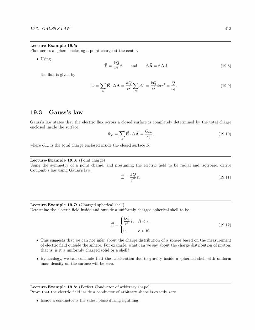
19.3. GAUSS’S LAW 413

Lecture-Example 19.5:Flux across a sphere enclosing a point charge at the center.

• Using

~E =kQ

r2r and ∆~A = r∆A (19.8)

the flux is given by

Φ =∑

S

~E ·∆A =kQ

r2

∑

S

dA =kQ

r24πr2 =

Q

ε0. (19.9)

19.3 Gauss’s law

Gauss’s law states that the electric flux across a closed surface is completely determined by the total chargeenclosed inside the surface,

ΦE =∑

S

~E ·∆~A =Qen

ε0, (19.10)

where Qen is the total charge enclosed inside the closed surface S.

Lecture-Example 19.6: (Point charge)Using the symmetry of a point charge, and presuming the electric field to be radial and isotropic, deriveCoulomb’s law using Gauss’s law,

~E =kQ

r2r. (19.11)

Lecture-Example 19.7: (Charged spherical shell)Determine the electric field inside and outside a uniformly charged spherical shell to be

~E =

kQ

r2r, R < r,

0, r < R.

(19.12)

• This suggests that we can not infer about the charge distribution of a sphere based on the measurementof electric field outside the sphere. For example, what can we say about the charge distribution of proton,that is, is it a uniformly charged solid or a shell?

• By analogy, we can conclude that the acceleration due to gravity inside a spherical shell with uniformmass density on the surface will be zero.

Lecture-Example 19.8: (Perfect Conductor of arbitrary shape)Prove that the electric field inside a conductor of arbitrary shape is exactly zero.

• Inside a conductor is the safest place during lightning.

414 CHAPTER 19. GAUSS’S LAW

Lecture-Example 19.9: (Structure of an atom)The electric field inside and outside a uniformly charged solid sphere of radius R and charge Q is given by

~E =

kQ

r2r, R < r,

kQr

R3r, r < R.

(19.13)

• Plot the magnitude of the electric field as a function of r.

• Discuss how this contributed to the Rutherford’s model for the structure of atom.

Lecture-Example 19.10:Consider a perfectly conducting sphere of radius R = 7.0 cm with charge Q = 1.0µC. Determine the electric fluxthrough the surface of a (Gaussian) sphere of radius 5.0 cm, concentric with respect to the conducting sphere.

Chapter 20

Electric potential energy and theelectric potential

20.1 Work done by the electric force

The electric force on a charge q in an electric field ~E is given by

~F = q~E. (20.1)

The work done by the electric force on charge q is given by

W = ~F · ~d = Fd cos θ = qEd cos θ, (20.2)

where ~d is the displacement and θ is the angle between the force and displacement.

Lecture-Example 20.1: Consider a region of uniform electric field ~E = −E j of magnitude E = 1.0×103N/Cand direction vertically down. Determine the work done by the electric force when a charged sphere with chargeq = 10.0µC is moved along a path. Let the vertical distance between points ‘1’ to ‘2’ be h = 10.0 cm.

1

2 3

~E


• The work done by the electric force when the particle moves along the path connecting points ‘1’ to ‘2’,‘2’ to ‘3’, and ‘3’ to ‘1’, are

W1→2 = −qEh, (20.3a)

W2→3 = 0, (20.3b)

W3→1 = qEh. (20.3c)

415

416 CHAPTER 20. ELECTRIC POTENTIAL ENERGY AND THE ELECTRIC POTENTIAL

• Further, the total work done by the electric force for the closed loop 1 → 2 → 3 → 1 is

W1→2→3→1 = 0. (20.4)

• Note that the work done is zero for a path that is perpendicular to the electric field. An arbitrary path canbe broken down into infinitely small vertical and horizontal displacements. Thus, for the case of uniformelectric field we can show that the work done is independent of the path and only depends on the initialand final points.

20.2 Electric potential energy

The work done by the electric force is zero for a closed path (in the absence of time varying magnetic fields).As a corollary, the work done by the electric force is completely determined by the initial and final points of thepath traversed. This is the statement of the electric force being a conservative force. For a conservative forceit is convenient to define an associated potential energy, in the statement of work-energy theorem. The electricpotential energy of a charge q in a uniform electric field created in between oppositely charged parallel plates,choosing the potential energy to be zero when the charge is at the negative plate, is

U = qEh, (20.5)

h being the distance of the charge from the negative plate. The electric potential energy of two charges q1 andq2, choosing the potential energy to be zero at infinity, is

U =kq1q2r

. (20.6)

Lecture-Example 20.2: (Point charges)A positive charge q2 is moved in the vicinity of a another positive charge q1. Determine the work done by theelectric force when the charge q2 is moved along a path.

1

2

3

4


• Evaluate the work done by the electric force on the charge q2 when it is moved along the path ‘1’ to ‘2’,‘2’ to ‘3’, ‘3’ to ‘4’, ‘4’ to ‘1’.

• Plot the electric potential energy U between two positive charges q1 and q2 as a function of r. Next, plotthe electric potential energy U between two unlike charges q1 and q2 as a function of r. Interpret theseplots as a statement of the fact that force is the manifestation of the system trying to minimize its energy.

20.2. ELECTRIC POTENTIAL ENERGY 417

• Equipotential surfaces are surfaces perpendicular to the electric field. The work done by the electric forceis zero while moving on equipotential surfaces.

Lecture-Example 20.3: (Energy required to assemble a set of charges)Show that the energy required to assemble three positive charges q1, q2, and q3, at relative distances r12, r23,and r31, is

U =kq1q2r12

+kq2q3r23

+kq3q1r31

. (20.7)

• Show that the total energy required to assemble three identical positive charges q at the corners of anequilateral triangle of side L is

U = 3kq2

L. (20.8)

• Show that the total energy required to assemble four identical positive charges q at the corners of a squareof side L is

U = (4 +√2)kq2

L. (20.9)

Lecture-Example 20.4:A sphere with mass m2 = 10 g and charge q2 = 1.0µC is fired directly toward another sphere of chargeq1 = 10.0µC (which is pinned down to avoid its motion). If the initial velocity of charge q2 is vi = 10.0m/swhen it is ri = 30 cm away from charge q1, at what distance away from the charge q1 does it come to rest?

• Using conservation of energy we have

kq1q2ri

+1

2m2v

2i =

kq1q2rf

+1

2m2v

2f . (20.10)

Answer: rf = 11 cm.

Lecture-Example 20.5:Two oppositely charged, parallel plates are placed d = 8.0 cm apart to produce an electric field of strengthE = 1.0× 103N/C between the plates. A sphere of mass m = 10.0 g and charge q = 10.0µC is projected fromone surface directly toward the second. What is the initial speed of the sphere if it comes to rest just at thesecond surface?

• Using conservation of energy we have1

2mv2 = qEd. (20.11)

Answer: v = 0.4m/s.


20.3 Electric potential

Electric potential energy per unit charge is defined as the electric potential. It is measured in units ofVolt=Joule/Coulomb. Thus,

∆U = q∆V. (20.12)

For a point charge, after choosing the electric potential to be zero at infinity, we have

V =kq

r. (20.13)

For uniform electric field created by oppositely charged parallel plates, after choosing the electric potential tobe zero at the negative plate, we have

V = Eh, (20.14)

h being the distance from the negative plate.

Lecture-Example 20.6:Two electrons and two protons are placed at the corners of a square of side 5 cm, such that the electrons are atdiagonally opposite corners.

• What is the electric potential at the center of square?

• What is the electric potential at the midpoint of either one of the sides of the square?

• How much potential energy is required to move another proton from infinity to the center of the square?

• How much additional potential energy is required to move the proton from the center of the square to oneof the midpoint of either one of the sides of the square?

Lecture-Example 20.7:Charges of −q and +2q are fixed in place, with a distance of a = 2.0m between them. See Fig. 20.3. A dashedline is drawn through the negative charge, perpendicular to the line between the charges.

y

a−q+2q


• On the dashed line, at a distance y from the negative charge, there is at least one spot where the totalpotential is zero. Find y. (Answer: y = ±a/

√3.)

• On the line connecting the charges, between the two charges, find the spot where the total potential iszero. (Answer: Distance a/3 to the right of −q charge.) On the line connecting the charges, to the left ofthe smaller charge, find the spot where the total potential is zero. (Answer: Distance a to the left of −qcharge.)

20.4. ELECTRIC POTENTIAL INSIDE A PERFECTLY CHARGED CONDUCTOR 419

• On the line connecting the charges, to the right of the larger charge, show that there is no spot wherethe total potential is zero. In general for α = q2/q1 < 0, remembering that the potential involves themagnitude of the distance, the two solutions on the line connecting the charges are contained as solutionsto the quadratic equation,

(α2 − 1)z2 + 2az − a2 = 0, (20.15)

which has solutions

z =a

1 + αand z =

a

1− α. (20.16)

• For like charges, α = q2/q1 > 0, there is no spot with zero potential other than infinity, because twopositive numbers can not add to give zero.

20.4 Electric potential inside a perfectly charged conductor

Since the electric field is zero inside a perfectly charged conductor, because otherwise the charges will experiencea force, the implication is that the electric potential is a constant inside the conductor.

Lecture-Example 20.8:Determine the electric potential inside and outside a perfectly conducting charged sphere of radius R. Plot this.

Lecture-Example 20.9: (Fork in a microwave)To illustrate why pointed metals spark inside a microwave, let us consider two conducting spheres of radius R1

and R2, connected by a conducting thread, but placed significantly away from each other.

• Using the fact that the electric potential is the same at the surface of the two spheres,

V1 = V2, (20.17)

show that the ratio of the charges on the two spheres is

Q1

Q2

=R1

R2

. (20.18)

Thus, the charge is proportional to the radius.

• Show that the ratio of the electric fields isE1

E2

=R2

R1

. (20.19)

Thus, the electric field is inversely proportional to the radius. This implies the smaller sphere will have alarger electric field near its surface. If the electric field is large enough to breakdown air, we see a spark.


20.5 Capacitor

The potential difference between two conducting objects, consisting of equal and opposite charge Q, is linearlydependent on the charge Q and the geometrical dependence on the shape of the objects can be absorbed intoa constant. In general, we have

V =Q

C, (20.20)

where the electric potential is chosen to be zero at the negative plate. The geometry dependent parameter C isdefined as the capacitance. For parallel plate configuration the capacitance is given by

C =ε0A

d, (20.21)

where A is the area of the individual plates and d is the distance between the plates.The total energy stored in a capacitor is given by

U =Q2

2C=

1

2CV 2, (20.22)

which is also the energy required to separate the charges. This energy is stored as the electric field in betweenthe plates,

U

Ad=

1

2ε0E

2. (20.23)

Lecture-Example 20.10: (A rudimentary capacitor)Cut out two strips of aluminum foil, A = 1 cm× 1m = 10−2m2. Place a sheet of paper in between the stripsand roll the sheets. Estimate the thickness of paper to be d = 100µm. The medium between the plates is paper,which has a permittivity of ε ∼ 3.9 ε0. Estimate the capacitance of this construction. (Answer: C ∼ 1 nF.)

• Traditional capacitors used in electrical circuits range between picofarad (pF) and microfarad (µF). Para-sitic capacitance, the unavoidable stray capacitance, is typically about 0.1 pF. More recently, capacitancegreater than kilofarad (kF) have been feasible, and are called supercapacitors.

Lecture-Example 20.11:The breakdown field strength of paper is about ten times that of air, Ec ∼ 107V/m. Determine the maximumenergy that can be stored in the rudimentary capacitor of Lecture-Example 20.10. (Answer: ∼ 1mJ.)

Chapter 21

Electric circuits

We have learned that positive charges tend to move from a point of higher electrical potential to a point of lowerelectrical potential, and negative charges tend to do the opposite. This basic idea is at the heart of electricalcircuits, which involves flow of electric charges. A traditional battery is a device that provides a (constant)potential difference, by moving charges against their natural tendency. The three basic electrical componentswill will discuss are: capacitor, resistor, and inductor.

21.1 Current

Flow of electric charges (in a conducting wire) is described by current,

I =∆q

∆t. (21.1)

It is measured in units of Ampere=Coulomb/second. It is expressed in terms of the number density of chargecarriers n, area of crosssection of the wire A, and drift velocity (speed of flow) vd, as

I = neAvd. (21.2)

Lecture-Example 21.1: (Drift velocity)Estimate the drift velocity in typical metals. Let us consider a current of I = 1A passing through a copperwire with area of crosssection A = πr2 = π(1mm)2 ∼ 3 × 10−6m2. Since Copper has one free electron peratom, density of 8.9 g/cm3, and atomic weight of 63.5 g/mole, we estimate n = 9× 1028 atoms/m3. (Avagadro’snumber is 6× 1023 atoms/mole.) (Answer: vd = 2× 10−5m/s.)

• How much time does it take for an individual electron to begin from the light switch to the bulb that isconnected by a 2m copper wire? (Answer: 28 hours.)

• To put on the light switch it is the flow that is relevant, very much like water arriving at the faucetinstantly.

21.2 Resistance

Resistance in a wire is the opposition to the flow of charges. For standard materials it is proportional to thelength of wire l, inversely proportional to area of crosssection A, in addition to it depending on the materialspecific property, the resistivity ρ. Together, we have

R =ρl

A. (21.3)

421

422 CHAPTER 21. ELECTRIC CIRCUITS

It is measured in units of Ohms=Volt/Ampere.

21.3 Ohm’s law

The current I flowing through a resistor R is directly proportional to the potential difference across the resistor,for many materials. This is the statement of Ohm’s law,

V = IR. (21.4)

21.4 Power dissipated in a resistor

The power dissipated in a resistor is given by

P = IV =V 2

R= I2R. (21.5)

21.5 Resistors in series and parallel

A resistor when connected to a battery leads to a flow of current. The current I is decided by the resistance Rand potential difference V across the resistor,

I =V

R. (21.6)

Lecture-Example 21.2:A resistor R = 500Ω is connected across a 10.0V battery. Determine the current in the circuit. (Answer:20mA.)

Resistors in series

Consider two resistors in series as described in Figure 21.1. Since the potential difference across the battery isdistributed across the two resistors we deduce that

V = V1 + V2. (21.7)

The current flowing both the resistors is the same,

I1 = I2, (21.8)

because the channel for flow does not bifurcate. An equivalent resistor Req shown on the right side in Figure 21.1is defined as a resistor that will pull the same amount of current from the battery. Thus, using V1 = I1R1,V2 = I2R2, and V = IeqReq, in Eq. (21.7), we learn that

Req = R1 +R2. (21.9)

We can further deduce thatV1

V2

=R1

R2

, (21.10)

which turns out to be handy in the analysis of more complicated configurations.

Lecture-Example 21.3: (Resistors in series)A potential difference V = 10.0V is applied across a resistor arrangement with two resistances connected inseries, R1 = 100.0Ω and R2 = 200.0Ω.

21.5. RESISTORS IN SERIES AND PARALLEL 423

V

R1

R2

V Req

Figure 21.1: Resistors in series.

• Find the equivalent resistance. (Answer: Req = 300.0Ω.)

• Find the currents I1 and I2 flowing through the resistors. (Answer: I1 = I2 = 33.3mA.)

• Find the voltages V1 and V2 across each of the resistors. (Answer: V1 = 3.33V and V2 = 6.67V.)

• Find the power P1 and P2 dissipated in each of the resistors. (Answer: P1 = 111mW and P2 = 222mW.)

Resistors in parallel

Consider two resistors in parallel as described in Figure 21.2. The potential difference across each resistor isidentical,

V = V1 = V2. (21.11)

The total current I that flows out of the battery distributes between the two resistors,

I = I1 + I2. (21.12)

An equivalent resistor Req shown on the right side in Figure 21.2 is defined as a resistor that will pull the sameamount of current from the battery. Thus, using I1 = V1/R1, I2 = V2/R2, and I = V/Req, in Eq. (21.12), welearn that

1

Req

=1

R1

+1

R2

. (21.13)

We can further deduce thatI1I2

=R2

R1

, (21.14)


V R1 R2 V Req

Figure 21.2: Resistors in parallel.

Lecture-Example 21.4: (Resistors in parallel)A potential difference V = 10.0V is applied across a resistor arrangement with two resistances connected inparallel, R1 = 100.0Ω and R2 = 200.0Ω.


• Find the equivalent resistance. (Answer: Req = 66.7Ω.)

• Find the voltages V1 and V2 across each of the resistors. (Answer: V1 = V2 = 10.0V.)

• Find the currents I1 and I2 flowing through each of the resistors. (Answer: I1 = 100mA and I2 = 50mA.)

• Find the power P1 and P2 dissipated in each of the resistors. (Answer: P1 = 1.00W and P2 = 0.500W.)

21.6 Capacitors in series and parallel

A capacitor when connected to a battery collects equal and opposite charges on its plates. The amount ofcharge Q it collects is decided by the capacitance C and potential difference V across the plates,

Q = CV. (21.15)

Lecture-Example 21.5:A capacitor of capacitance C = 10µF is connected across a 10.0V battery. Determine the charge accumulatedon the plates of the capacitor. (Answer: 100µC.)

Capacitors in series

Consider two capacitors in series as described in Figure 21.3. Since the potential difference across the batteryis distributed across the two capacitors we deduce that

V = V1 + V2. (21.16)

The charges on each of the capacitors will be identical,

Q1 = Q2, (21.17)

because by construction the part of circuit between the two capacitors is isolated. An equivalent capacitor Ceq

shown on the right side in Figure 21.3 is defined as a capacitor that will collect the same amount of charge fromthe battery. Thus, using V1 = Q1/C1, V2 = Q2/C2, and V = Qeq/Ceq, in Eq. (21.16), we learn that

1

Ceq

=1

C1

+1

C2

. (21.18)

We can further deduce thatV1

V2

=C2

C1

, (21.19)


Lecture-Example 21.6: (Capacitors in series)A potential difference V = 10.0V is applied across a capacitor arrangement with two capacitances connectedin series, C1 = 10.0µF and C2 = 20.0µF.

• Find the equivalent capacitance. (Answer: Ceq = 6.67µF.)

• Find the charges Q1 and Q2 on each of the capacitors. (Answer: Q1 = Q2 = 66.7µC.)

• Find the voltages V1 and V2 across each of the capacitors. (Answer: V1 = 6.67V and V2 = 3.33V.)

• Find the potential energies U1 and U2 stored inside each of the capacitors. (Answer: U1 = 222µJ andU2 = 111µJ.)

21.6. CAPACITORS IN SERIES AND PARALLEL 425

V

C1

C2

V Ceq

Figure 21.3: Capacitors in series.

Capacitors in Parallel

Consider two capacitors in parallel as described in Figure 21.4. The potential difference across each capacitoris identical,

V = V1 = V2. (21.20)

The total charge Q that is pulled out of the battery distributes on the two capacitors,

Q = Q1 +Q2. (21.21)

An equivalent capacitor Ceq shown on the right side in Figure 21.4 is defined as a capacitor that will collect thesame amount of charge from the battery. Thus, using Q1 = V1C1, Q2 = V2C2, and Q = V Ceq, in Eq. (21.21),we learn that

Ceq = C1 + C2. (21.22)

We can further deduce thatQ1

Q2

=C1

C2

, (21.23)


V C1 C2 V Ceq

Figure 21.4: Capacitors in parallel.

Lecture-Example 21.7: (Capacitors in parallel)A potential difference V = 10.0V is applied across a capacitor arrangement with two capacitances connectedin parallel, C1 = 10.0µF and C2 = 20.0µF.

• Find the equivalent capacitance. (Answer: Ceq = 30.0µF.)

• Find the voltages V1 and V2 across each of the capacitors. (Answer: V1 = V2 = 10.0V.)

• Find the charges Q1 and Q2 on each of the capacitors. (Answer: Q1 = 0.100mC and Q2 = 0.200mC.)

• Find the potential energies U1 and U2 stored inside each of the capacitors. (Answer: U1 = 0.500mJ andU2 = 1.00mJ.)

Chapter 22

Magnetic force

22.1 Magnetic field

The concepts introduced in electrostatics can be summarized in the following symbolic form:

Charge q1 → Electric field (~E1) → Charge q2 feels a force ~F21 = q2~E1

That is, a charge q1 creates an electric field ~E1 which exerts a force ~F21 on another charge q2. A moving charge,in addition to the above, leads to a new phenomenon. A moving charge creates a magnetic field which exerts aforce on another moving charge. This is summarized in the form:

Moving charge q1~v1 → Magnetic field (~B1) → Moving charge q2~v2 feels a force ~F21 = q2~v2 × ~B1

Thus, a charge q moving with velocity ~v, represented by

q~v (22.1)

or the corresponding current due to the movement of the charge, is a source of magnetic field. A manifestationof this phenomena at the microscopic level is seen in the interaction of two magnets, where the magnetic fielddue to one magnet exerts a force on the second magnet.

The Magnetic field is measured in units of Tesla=N·s/C·m. The common magnetic fields we come across islisted in Table 22.1.

22.2 Magnetic force

The force on a charge q moving with velocity ~v in a magnetic field ~B is symbolically given by

~F = q~v × ~B. (22.2)

108T magnetic field of a neutron star102T strength of a laboratory magnet101T medical MRI100T a neodymium magnet10−3T a refrigerator magnet10−4T strength on surface of Earth10−12T human brain

Table 22.1: Orders of magnitude (magnetic field)

427

428 CHAPTER 22. MAGNETIC FORCE

The magnitude of the magnetic force ~F is given by

F = qvB sin θ, (22.3)

and the direction of the force is given by the right-hand rule. The right-hand rule is a mnemonic that associatesthe thumb to the velocity vector, the fingers to the magnetic field, and the force in the direction facing the palmof the right hand. The right-hand rule applies to a positive charge. For a negative charge the direction of forceis flipped.

In discussions concerning the magnetic force we often have quantities pointing in and out of a plane. Weshall use the notation

⊙

to represent a direction coming out of the plane, and⊗

to represent a direction goinginto the plane. As a mnemonic one associates the dot with the tip of an arrow coming out of the page and thecross with the feathers of an arrow going into the page.

Lecture-Example 22.1:A proton and an electron enters a region containing a magnetic field going into the page, ~B = −2.0 zT. Let thevelocity of both the particles while they enter the region be to the right, ~v = 3.0× 105 xm/s.

• Determine the magnitude of the magnetic force on the proton and the electron.

• Determine the direction of the magnetic force on the proton and the electron, using the right-hand rule.

• Determine the corresponding accelerations experienced the proton and the electron.

22.3 Motion of a charged particle in a uniform magnetic field

In a uniform magnetic ~B, if the velocity of a particle ~v is perpendicular to the direction of the magnetic field,the direction of the acceleration of the particle is always perpendicular to the velocity of the particle and tothe magnetic field. Further, for the case of uniform magnetic field the magnitude of the acceleration remainsconstant. These are the requirements for a particle to move in a circle with uniform speed. Thus, using Newton’slaw, F = ma, for circular motion, we have

qvB = mv2

R, (22.4)

where R is the radius of the circle and ω is the angular frequency of the rotational motion, such that wherev = ωR. We learn that the particle particle goes around the magnetic field at an angular frequency, the cyclotronfrequency, given by

ω =q

mB, (22.5)

which depends on the charge to mass ratio of the particle.For the more general case of the velocity not being perpendicular to the magnetic field the particle drifts in

the direction of the magnetic field while moving in circles, the path covered being helical.

Lecture-Example 22.2: (Northern lights)A proton and an electron are moving in circles around a magnetic field of B = 1.0× 10−6T.

• Determine the cyclotron frequency for the proton and the electron.(Answer: ωp = 96 rad/s, ωe = 1.8× 105 rad/s.)

• If the particles are moving with uniform speed v = 2.0 × 106m/s, determine the radius of the circlesdescribing their path. (Answer: Rp = 21km, Re = 11m.)

22.4. MAGNETIC FORCE ON A CURRENT CARRYING WIRE 429

• Aurora Borealis (northern lights) and Aurora Australis (southern lights) is a spectacular display of lightshimmering across the night sky, often observed aroundmagnetic poles of the Earth, when charged particlesemitted by the Sun and guided along by the magnetic field of the Earth enter the atmosphere. Check outan animation of this phenomenon as seen from space, released by NASA Earth Observatory,

Aurora Australis on 2005 Sep 11,

which to an observer on Earth would appear as a curtain of shimmering light.

Lecture-Example 22.3: (Bubble chamber)Refer to the following tutorial at CERN: How to read Bubble Chamber pictures.

Lecture-Example 22.4: (Velocity selector)The electric field and the magnetic field both deflect charged particles due to the respective forces. In a velocityselector these forces are exactly balanced for particles moving with a particular velocity which go throughundeviated. Show that the velocity of a velocity selector is determined by

v =E

B. (22.6)

• Determine the velocity selected by a velocity selector consisting of an electric field of E = 3.0× 105N/Cand a magnetic field of B = 1.5T. (Answer: v = 2.0× 105 m/s.)

Lecture-Example 22.5: (Applications)

• Mass spectrometer

• Hall effect

• Cyclotron

• Cathode ray tube

22.4 Magnetic force on a current carrying wire

Using the fact that a current carrying wire involves the motion of positive positive charges we realize that thewire will experience a magnetic force in a magnetic field. Identifying the relation

qv = qL

t= IL, (22.7)

where I is the current in the wire, we derive the force on a current carrying wire of length L to be

F = ILB sin θ. (22.8)

The direction of the force is given using the right-hand rule with the thumb in the direction of current.

Lecture-Example 22.6:A loop in the shape of a right triangle, carrying a current I, is placed in a magnetic field. (Choose z to be outof the page.)

https://en.wikipedia.org/wiki/File:Aurora_Australis.gif

http://teachers.web.cern.ch/teachers/archiv/HST2005/bubble_chambers/BCWebsite/index.htm


x

y I

1

2

3~B

θ


• The force on side 1 is given by~F1 = IBx sin 180 z = 0 z. (22.9)

The force on side 2 is given by~F2 = −IBy sin 90 z = −IBy z. (22.10)

The force on side 3 is given by, using sin θ = y/√

x2 + y2,

~F3 = IB√

x2 + y2 sin θ z = IBy z. (22.11)

• Show that the total force on the triangle is zero.

Lecture-Example 22.7:A loop in the shape of a right triangle, carrying a current I, is placed in a magnetic field. (Choose z to be outof the page.)

×

×

×

×

×

×

×

×

×

×

×

×

×

×

×

×

×

×

×

×

×

×

×

×x

y I

1

2

3~B

θ


• The force on side 1 is given by~F1 = −IBx sin 90 y = −IBx y. (22.12)

The force on side 2 is given by~F2 = −IBy sin 90 x = −IBy x. (22.13)

The force on side 3 is given by, using sin θ = y/√

x2 + y2,

~F3 = IB√

x2 + y2 sin θ x+ IB√

x2 + y2 cos θ y = IBy x+ IBx y. (22.14)

• Show that the total force on the triangle is zero.

22.5. MAGNETIC MOMENT OF A CURRENT CARRYING LOOP 431

22.5 Magnetic moment of a current carrying loop

The magnetic moment ~µ associated with a (planar) current carrying loop of wire is

~µ = NIA n, (22.15)

where I is the current in the wire, N is the number of turns in the loop, and A is the area of the loop. Thedirection of the magnetic moment, represented by n, is perpendicular to the plane constituting the loop and isgiven by the right-hand rule. An arbitrary shaped loop that is not planar can be constructed out of infinitelysmall planar loops.

A magnet is interpreted to have a North and South pole, in the Gilbert model. In the Ampere modelthe magnetic field due to a magnet is due to microscopic current loops. The magnetic moment of a magnetcharacterizes the strength of a magnetic field produced by the magnet.

Force

The total force on a current carrying loop in a uniform magnetic field is zero.

Torque

The magnitude of the torque on a current carrying loop, or just a magnetic moment ~µ, in a uniform magneticfield ~B, is

τ = µB sin θ, (22.16)

where θ is the angle between the direction of the magnetic moment ~µ and the magnetic field ~B. The directionis such that the magnetic moment tries to align with the magnetic field.

Lecture-Example 22.8:A loop in the shape of a rectangle, carrying a current I, is placed in a magnetic field. Let the plane of the loopbe perpendicular to the magnetic field ~B = −B z.

×

×

×

×

×

×

×

×

×

×

×

×

×

×

×

×

×

×

×

×

×

×

×

×

×

×

×

×Lx

Ly

I

1

2

3

4

~B

⊙ x

y

zLy

⊙

⊗ 1

4

3

2

~B

⊙z

y

x


• The force on side 1 is given by

~F1 = −y ILxB sin 90 = −y ILxB. (22.17)

The force on side 2 is given by

~F2 = −x ILyB sin 90 = −x ILyB. (22.18)


~F3 = +y ILxB sin 90 = +y ILxB. (22.19)



~F4 = +x ILyB sin 90 = +x ILyB. (22.20)

• Show that the total force on the rectangle is zero.

• Show that the total torque on the rectangle is zero.

Lecture-Example 22.9:A loop in the shape of a rectangle, carrying a current I, is placed in a magnetic field. Let the normal to theplane of the loop make an angle θ with respect to the magnetic field ~B = −B z.

×

×

×

×

×

×

×

×

×

×

×

×

×

×

×

×

×

×

×

×

×

×

×

×

×

×

×

×Lx

Ly

I

1

2

3

4

~B

⊙ x

y

z⊙

⊗

Ly

~µ

θ

1

4

3

2

~B

⊙z

y

x


• The force on side 1 is given by

~F1 = −y ILxB sin 90 = −y ILxB. (22.21)


~F2 = −x ILyB sin(90 + θ) = −x ILyB cos θ. (22.22)


~F3 = +y ILxB sin 90 = +y ILxB. (22.23)


~F4 = +x ILyB sin(90 − θ) = +x ILyB cos θ. (22.24)

• Show that the total force on the rectangle is zero.

• Show that the total torque on the rectangle is

τ =Ly

2F3 sin θ +

Ly

2F1 sin θ = µB sin θ. (22.25)

Chapter 23

Magnetic field due to currents

23.1 Magnetic field due to currents

A straight segment of wire

The magnetic field due to a straight segment of wire at a distance r from the wire is

B =µ0I

4πr(sin θ1 + sin θ2), (23.1)

where the angles θ1 and θ2 specifies the observation point with respect to the ends of the wire. See Figure 23.1.The direction of the magnetic field is given by the right-hand rule. As a special case, we have the magnetic field

I

rθ2

θ1⊗

Figure 23.1: A straight segment of wire.

due to an infinitely long wire, θ1 = θ2 = π/2, as

B =µ0I

2πr. (23.2)

The constant µ0 is the permeability of vacuum,

µ0 = 4π × 10−7 T·mA

. (23.3)

A circular segment of wire

The magnetic field due a circular segment of wire, at the center of circle, is

B =µ0I

4πRθ, (23.4)

where the angle θ is the angular measure of the segment. See Figure 23.2. The direction of the magnetic fieldis given by the right-hand rule. As a special case, we have the magnetic field due to a circular loop of wire,

433

434 CHAPTER 23. MAGNETIC FIELD DUE TO CURRENTS

I

R

θ ⊗

Figure 23.2: A straight segment of wire.

θ = 2π, at the center of the loop, as

B =µ0I

2R. (23.5)

Solenoid

The magnetic field inside a solenoid of infinite extent is uniform, and zero outside. In particular,

B =

µ0In, inside,

0, outside,(23.6)

where n = N/L is the number of turns N per unit length L.

Lecture-Example 23.1: A steady current I flows through a wire shown in Fig. 23.3. Show that the magnitudeand direction of magnetic field at point P is

B =µ0I

4πa

(

2

2+

2

2+

2π

2

)

(23.7)

coming out of the page.

b

P~v

a I


• Determine the magnitude and direction of the magnetic field for I = 1.0A and a = 10.0 cm.

• Determine the magnitude and direction of the magnetic force on a proton moving with velocity v =2.0× 106 m/s, to the right, while it is passing the point P .

Lecture-Example 23.2: A steady current I flows through a wire shown in Fig. 23.4. Show that the magnitudeand direction of magnetic field at point P is

B =µ0I

4πa

(

2

2+

2

2+

2π

4

)

(23.8)

23.1. MAGNETIC FIELD DUE TO CURRENTS 435

b P

a I


going into the page.

• Determine the magnitude and direction of the magnetic field for I = 1.0A and a = 10.0 cm.

• Determine the magnitude and direction of the magnetic force on a proton moving with velocity v =2.0× 106 m/s, to the right, while it is passing the point P .

Lecture-Example 23.3: A steady current I flows through a wire in the shape of a square of side L, shownin Fig. 23.5. Show that the magnitude and direction of the magnetic field at the center of the square, P , is

B =µ0I

πL

4√2

(23.9)

going out of the page.

b P

I


Lecture-Example 23.4:Figure 23.6 shows two current carrying wires, separated by a distance D. The directions of currents, eithergoing into the page or coming out of the page, are shown in the figure. Determine the point × where themagnetic field is exactly zero.

• Answer:

x =D

(

1 + I2I1

) . (23.10)

Determine x if I1 = 2.0A, I2 = 6.0A, and D = 10.0 cm. (Answer: 2.5A.)

• How does your answer change if the direction of currents in either or both the wires were changed?


×I1 I2

D

x


Lecture-Example 23.5:Figure 23.7 shows two current carrying wires, in a plane. The directions of currents, either going into the pageor coming out of the page, are shown in the figure. Determine the magnitude and direction of the magneticfield at the point ×, the origin. Let I1 = 1.0A, I2 = 2.0A, x = 12 cm, and y = 8.0 cm.

××

I1

I2x

y


• The magnetic field at the origin due to the individual wires is

~B1 =µ0I12πy

i+ 0 j, (23.11a)

~B2 = 0 i+µ0I22πx

j. (23.11b)

The total magnetic field is given as~Btot = ~B1 + ~B2. (23.12)

Answer: ~B1 = i 2.5µT and ~B2 = j 3.3µT. Magnitude |~Btot| = 4.1µT makes an angle of 53 counter-clockwise with respect to x-axis.

• How does your answer change if the direction of currents in either or both the wires were changed?

Lecture-Example 23.6:A 200 turn solenoid having a length of 20.0 cm and a diameter of 1.0 cm carries a current of 1.0A. Calculatethe magnitude of the magnetic field B inside the solenoid.

• Since the diameter is sufficiently less than the length of the solenoid we can approximate the solenoid tobe of infinite length. (Answer: B = 1.3mT.)

23.2. FORCE BETWEEN PARALLEL CURRENT CARRYING WIRES 437

23.2 Force between parallel current carrying wires

If we have two parallel current carrying wires, each of the wires generates a magnetic field around it, which inturn exerts a force on the other wire. For currents I1 and I2 in the wires separated by a distance r we have theforce per unit length on the wires given by

F

L=

µ0I1I22πr

. (23.13)

The direction of the force is such that the wires attract if the current are in the same direction, and vice versa.We say, like currents attract and unlike current repel.

Lecture-Example 23.7:Two infinitely long parallel wires, carrying currents I1 = 1.0A and I2 = 2.0A in the same direction, areseparated by a distance r = 10 cm.

• Determine the magnitude and direction of the magnetic field ~B1 generated by the current I1 at the positionof current I2. (Answer: B1 = 2.0µT.) Determine the magnitude and direction of the force exerted by the

magnetic field ~B1 on the wire with current I2. (Answer: 4.0µN.)

• How will the answer differ if the currents are in opposite directions?

Lecture-Example 23.8:A rectangular loop of wire carrying current I2 = 2.0A is placed near an infinitely long wire carrying currentI1 = 1.0A, such that two of the sides of the rectangle are parallel to the current I1. Let the distances bea = 5.0 cm, b = 4.0 cm, and l = 10.0 cm.

I2

I1a

l

b

1

2

3

4


• Determine the force on side ‘1’ of the loop. (Answer: 0.44µN away from the current carrying wire I1.)Determine the force on side ‘3’ of the loop. (Answer: 0.80µN towards the current carrying wire I1.)Further, show that the combined force on side ‘2’ and ‘3’ is zero. Determine the magnitude and directionof the total force on the loop. (Answer: 0.36µN towards the current carrying wire I1.)

• How does your analysis change if either of the currents were reversed?

23.3 Ampere’s law

Ampere’s law states that the total sum of the magnetic field ~B along a closed path is completely determinedby the total current Ien passing through the closed path,

∑

B∆l cos θ = µ0Ien. (23.14)


Lecture-Example 23.9: (Magnetic field due to an infinitely long current carrying wire)Using the symmetry of an infinitely long straight wire, presuming the magnetic field to be circular, derive themagnetic field around the wire using Ampere’s law,

~B = φµ0I

2πr. (23.15)

Lecture-Example 23.10: (Solenoid)Using Ampere’s law show that the magnetic field due to a solenoid is given by,

~B =

zµ0In, inside,

0, outside.(23.16)

Chapter 24

Faraday Induction

24.1 Magnetic flux

Flux associated with the magnetic field ~B across an infinitesimal area A is defined as

ΦB = BA cos θ, (24.1)

where θ is the angle between the vectors. Gauss’s law for magnetism states that the magnetic flux across aclosed surface is zero, that is

ΦB

∣

∣

∣

closed surface= 0, (24.2)

which implies the absence of an isolated magnetic monopole, or the magnetic charge. In other words it statesthat the north pole and the south pole of a bar magnet can not be separated.

Lecture-Example 24.1: A square loop of wire consisting of a single turn is perpendicular to a uniformmagnetic field. The square loop is then re-formed into a circular loop and is also perpendicular to the samemagnetic field. Determine the ratio of the flux through the square loop to the flux through the circular loop.(Answer: π/4.)

24.2 Faraday’s law of induction

Faraday’s law of induction states that the negative rate of change of magnetic flux passing a loop of wire inducesan effective voltage in the loop, which in turn generates a current in the loop,

IR = ∆Veff = −N∆φB

∆t, (24.3)

where N is the number of loops.

Lecture-Example 24.2:Consider a straight wire of length L = 1.0m moving with velocity v = 30.0m/s in the region of a uniformmagnetic field B = 2.0 × 10−5T. Determine the potential difference induced between the ends of the wire.(Answer: 0.60mV.)

Lecture-Example 24.3: (Induction due to change in area)

439

440 CHAPTER 24. FARADAY INDUCTION

×

×

×

×

×

×

×

×

×

×

×

×

×

×

×

×

×

×

×

×

×

×

×

×

v lR

B


Figure 24.1 shows a conducting a rod being pulled along horizontal, frictionless, conducting rails at a constantspeed v. A uniform magnetic field B fills the region in which the rod moves. Let l = 10 cm, v = 5.0m/s,B = 1.2T, and R = 0.40Ω.

• Is the magnetic flux in the loop increasing or decreasing? What is the direction of the induced current inthe loop?

• Show that the magnitude of the induced current in the loop is given by

I =Blv

R. (24.4)

Show that this induced current feels a magnetic force of

FB =B2l2v

R. (24.5)

Determine the power delivered to the resistance due to the induced current is

P =B2l2v2

R. (24.6)

• How does the analysis change if the direction of velocity is reversed?

Lecture-Example 24.4:Figure 24.2 shows five snapshots of a rectangular coil being pushed across the dotted region where there is auniform magnetic field directed into the page. Outside of this region the magnetic field is zero.

• Determine the direction of induced current in the loop at each of the five instances in the figure.

• Determine the direction force on the loop due to the induced current in each of the five instances in thefigure.

Lecture-Example 24.5: (Induction due to change in magnetic field)A loop of wire having a resistance R = 100.0Ω is placed in a magnetic field whose magnitude is changing intime, as described in Figure 24.3. The direction of the magnetic field is normal to the plane of the loop. Theloop of wire consists of 50 turns and has an area of A = 25× 10−4m2.

24.2. FARADAY’S LAW OF INDUCTION 441

×

×

×

×

×

×

×

×

×

×

×

×

×

×

×

×

×

×

×

×

×

×

×

×

B

v v v v v


0

1

2

2 4

t (in s)

B (in T)


• Determine the induced voltage and the induced current in the loop between 0 s to 2 s. (Answer: V = 0.13Vand I = 1.3mA.) Determine the induced voltage and the induced current in the loop between 2 s to 4 s.(Answer: V = 0 and I = 0.) Determine the induced voltage and the induced current in the loop between4 s to 5 s. (Answer: V = 0.25V and I = 2.5A.)

Lecture-Example 24.6: (A simple transformer)Consider two coils wound on the same cylinder such that the flux through both the coils is the same, such that

∆Φ1

∆t=

∆Φ2

∆t. (24.7)

Thus, derive the ratio of the voltages in the two coils to be given by

V1

V2

=N1

N2

. (24.8)

Energy conservation requires the power in the coils to be the same, that is P1 = P2. Thus, further derive

I2I1

=N1

N2

. (24.9)

A device operates at V2 = 10.0V. It uses a transformer to get the required voltage when plugged into a wallsocket with voltage V1 = 120V. Determine the ratio of the turns in the two coils inside the transformer. (Answer:N1/N2 = 12.) If the device pulls a current of 120mA, determine the current coming out of the wall socket.(Answer: I1 = 10mA.)

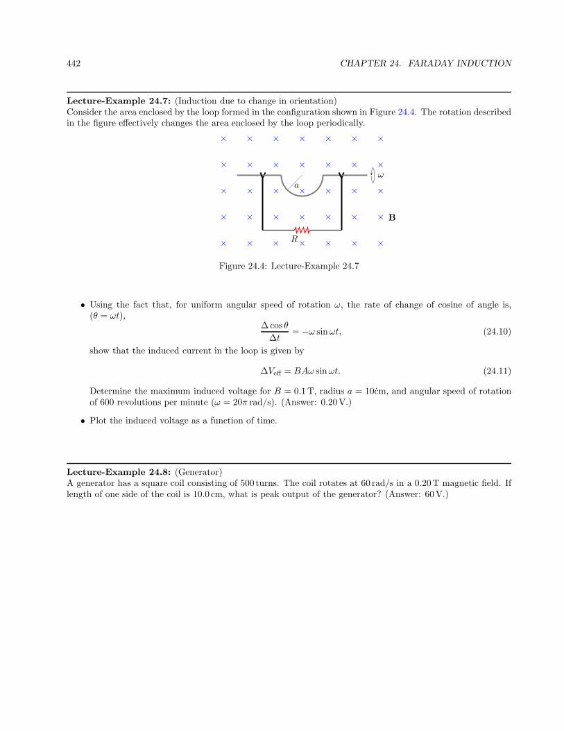
442 CHAPTER 24. FARADAY INDUCTION

Lecture-Example 24.7: (Induction due to change in orientation)Consider the area enclosed by the loop formed in the configuration shown in Figure 24.4. The rotation describedin the figure effectively changes the area enclosed by the loop periodically.

×

×

×

×

×

×

×

×

×

×

×

×

×

×

×

×

×

×

×

×

×

×

×

×

×

×

×

×

×

×

×

×

×

×

×R

B

ωa


• Using the fact that, for uniform angular speed of rotation ω, the rate of change of cosine of angle is,(θ = ωt),

∆ cos θ

∆t= −ω sinωt, (24.10)

show that the induced current in the loop is given by

∆Veff = BAω sinωt. (24.11)

Determine the maximum induced voltage for B = 0.1T, radius a = 10cm, and angular speed of rotationof 600 revolutions per minute (ω = 20π rad/s). (Answer: 0.20V.)

• Plot the induced voltage as a function of time.

Lecture-Example 24.8: (Generator)A generator has a square coil consisting of 500 turns. The coil rotates at 60 rad/s in a 0.20T magnetic field. Iflength of one side of the coil is 10.0 cm, what is peak output of the generator? (Answer: 60V.)

Chapter 25

Inductance

25.1 Self inductance

A coil of wire is the simplest example of an inductor. In general, a current carrying wire, of arbitrary shape, isan inductor. The potential difference across an inductor is linearly proportional to the rate of change of currentin the wire and the geometrical dependence on the shape of the wire can be absorbed into a constant. Thus,we have

V = L∆I

∆t. (25.1)

The geometry dependent parameter L is defined as the inductance. For a coil of length l, area of crosssectionA, and number of turns N , we have

L =µ0N

2A

l. (25.2)

Inductance is measured in units of Henry = Joule/Ampere2. The energy stored in an inductor is given by

U =1

2LI2. (25.3)

This energy is stored in the inductor in the form of magnetic field. Show that the energy density uB inside theinductor is

uB =1

2µ0

B2. (25.4)

Lecture-Example 25.1: (Inductance of a solenoid.)A solenoid of length l = 5.0 cm and radius r = 0.50 cm has N = 1000 turns. Determine the inductance of thesolenoid. (Answer: 2.0mH.)

25.2 RL circuit

A resistor and inductor in series constitutes a RL circuit. An inductor resists a change in current. Thus, it isthe inertia of current. An obvious scenario when sharp changes in current occur in a circuit is when the switchis turned on or off. An inductor in these instances smoothen the changes in currents.

443

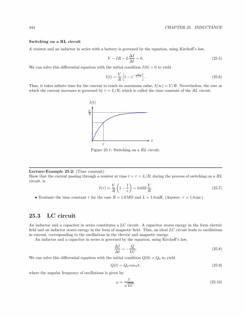
444 CHAPTER 25. INDUCTANCE

Switching on a RL circuit

A resistor and an inductor in series with a battery is governed by the equation, using Kirchoff’s law,

V − IR − L∆I

∆t= 0. (25.5)

We can solve this differential equation with the initial condition I(0) = 0 to yield

I(t) =V

R

[

1− e−t

L/R

]

. (25.6)

Thus, it takes infinite time for the current to reach its maximum value, I(∞) = V/R. Nevertheless, the rate atwhich the current increases is governed by τ = L/R, which is called the time constant of the RL circuit.

t

I(t)

τ

VR

Figure 25.1: Switching on a RL circuit.

Lecture-Example 25.2: (Time constant)Show that the current passing through a resistor at time t = τ = L/R, during the process of switching on a RLcircuit, is

I(τ) =V

R

(

1− 1

e

)

∼ 0.632V

R. (25.7)

• Evaluate the time constant τ for the case R = 1.0MΩ and L = 1.0mH. (Answer: τ = 1.0ms.)

25.3 LC circuit

An inductor and a capacitor in series constitutes a LC circuit. A capacitor stores energy in the form electricfield and an inductor stores energy in the form of magnetic field. Thus, an ideal LC circuit leads to oscillationsin current, corresponding to the oscillations in the electric and magnetic energy.

An inductor and a capacitor in series is governed by the equation, using Kirchoff’s law,

∆I

∆t= − Q

LC. (25.8)

We can solve this differential equation with the initial condition Q(0) = Q0 to yield

Q(t) = Q0 cosωt, (25.9)

where the angular frequency of oscillations is given by

ω =1√LC

. (25.10)

Chapter 26

Electromagnetic waves

26.1 Maxwell’s equations

Let us analyse the Ampere law for a RC circuit, while the capacitor is charging. Using Ampere’s law in Fig. 26.1,and using the ambiguity in defining the surface bounded by a curve, we deduce

V

R

C

S1

S2

Figure 26.1: Ampere’s law for an RC circuit.

∑

~B ·∆~l =

µ0I, for surface S1,

0, for surface S2.(26.1)

This apparent contradiction was removed by Maxwell by restating the Ampere law as

∑

~B ·∆~l = µ0I + µ0ε0∆ΦE

∆t, (26.2)

which implies that a rate of change of the electric flux can also generate a magnetic field.Thus, the four independent laws that govern the electric and magnetic field in a region of space, in integral

form, are the following.

∑

~E ·∆~A =Qen

ε0(Gauss’s law for ~E) (26.3a)

∑

~B ·∆~A = 0 (Gauss’s law for ~B) (26.3b)

∑

~E ·∆~l = ∆ΦB

∆t(Faraday’s law) (26.3c)

∑

~B ·∆~l = µ0ε0∆ΦE

∆t+ µ0I (Ampere’s law) (26.3d)

445

446 CHAPTER 26. ELECTROMAGNETIC WAVES

The above four equations are collectively called the Maxwell equations. The symmetry in the electric andmagnetic effects is striking in the above equations, which would have been complete if not for the absence ofmagnetic charges and magnetic currents. There is no conclusive experimental observation of magnetic charges.

26.2 Electromagnetic waves

The Maxwell equations imply that, in a region of space where there are no charges and currents, the electricand magnetic fields satisfy the wave equations

∆2~E

∆z2=

1

c2∆2~E

∆t2, (26.4a)

∆2~B

∆z2=

1

c2∆2~B

∆t2, (26.4b)

where the speed of these waves, called the speed of light, is

c =1√µ0ε0

. (26.5)

The meter, in SI units, is defined as the distance travelled by light in vacuum in 1/299 792 458 of a second. Asa consequence, the speed of light in vacuum, in SI units, is expressed as a whole number,

c = 299 792 458m

s. (26.6)

These electromagnetic waves, which are oscillations of the electric and magnetic fields in space and time, cansustain each other.

Properties of electromagnetic waves in vacuum

1. The wave nature stipulates the relation between the wavelength λ, frequency f , and speed c of the wave,

c = λf. (26.7)

The time period T = 1/f , and the wavevector k = 2π/λ, are related quantities.

2. The electromagnetic energy density is given by

u =1

2ε0E

2 +1

2µ0

B2. (26.8)

The flux of the electromagnetic energy density, a measure of the flow rate of electromagnetic energy perunit area, is given by the Poynting vector

~S =1

µ0

~E× ~B. (26.9)

The electromagnetic momentum density is given by

~G =1

c2~S. (26.10)

3. The Maxwell equations constraint the directions of the electric field, the magnetic field, and the directionof propagation to be mutually perpendicular,

~E× ~B = k cµ0u, ~E · ~B = 0. (26.11)

Further, we haveE = cB. (26.12)

26.3. DOPPLER EFFECT 447

Frequency Wavelength105Hz 103m AM radio wave108Hz 100m FM radio wave1011Hz 10−3m Microwave1015Hz 10−6m Visible light1017Hz 10−9m X ray1023Hz 10−15m Gamma ray

Table 26.1: Orders of magnitude (electromagnetic wave)

Lecture-Example 26.1: (Absorption coefficient of liquid water)Using the absorption coefficient of water as a function of frequency presented in the following link

http://www.britannica.com/science/absorption-coefficient/images-videos

argue that kilometer long waves (extremely low-frequency waves) are suitable candidates for communicationsbetween land base and submarines. (Inverse of absorption coefficient is a measure of how deep the wave willtravel in water before getting absorbed.)

Lecture-Example 26.2: (X-ray telescope)Using the opacity of electromagnetic waves as a function of the wavelength of eleactromagnetic waves presentedin the following link

Wikipedia: Opacity of atmosphere to electromagnetic waves

argue that an X-ray telescope has to be necessarily installed, above the atmosphere, in space. Further, discussradio-wave astronomy and gamma-ray astronomy.

26.3 Doppler effect

The Doppler formula for the apparent frequency measured by the observer, due to relative motion of the observerand source with respect to the medium, is given by

f ′ = f

(

v0 ± vdv0 ∓ vs

)

, (26.13)

where v0 is the speed of the wave, vs is the speed of the source, and vd is the speed of the detector. Thenon-relativistic Doppler formula for light, which does not take care of time dilation of special relativity, andapplicable to O(u/c)2, is

f ′ = f

(

1± |u|c

)

, (26.14)

where u = vs − vd is the relative velocity of the source with respect to the detector.

Lecture-Example 26.3: (Radar speed gun)A radar speed gun is a device that measures the relative speed of an object with respect to the device using theDoppler effect. Consider the case of a police car moving at 30.0m/s chasing a speeder moving at 40.0m/s. Theradar speed gun in the police car emits a radio signal with a frequency of 32.00GHz. Determine the differencein the emitted and detected frequencies of the radio signal as measured, by the radar gun after it has beenreflected off the speeding car. (Answer: 2135Hz.)

http://www.britannica.com/science/absorption-coefficient/images-videos

https://en.wikipedia.org/wiki/Electromagnetic_radiation#/media/File:Atmospheric_electromagnetic_opacity.svg

448 CHAPTER 26. ELECTROMAGNETIC WAVES

26.4 Polarization of an electromagnetic wave

The electric and magnetic field, the physical quantities that are oscillating in an electromagnetic wave, arevectors. When projected along a certain direction vectors collapse into their respective vector componentalong the direction, determined by the property of the scalar product of vectors. The polarization of a vectoris determined by the direction of the electric field of the electromagnetic wave. A polarizer is a device thatprojects the electric field along the direction of the transmission axis specific to the polarizer. The intensity of anelectromagnetic wave is proportional to the square of the electric field. Thus, the intensity of an electromagneticwave after passing through a polarizer is related to the intensity of the original wave by the relation

I ′ =

12I0, (for unpolarized incident wave),

I0 cos2 θ, (for polarized incident wave),

(26.15)

where θ is the relative orientation of the incident polarized wave with respect to the transmission axis of thepolarizer. The factor of half for the case of unpolarized light is the average of cos2 θ over angle θ.

Lecture-Example 26.4:Figure 26.2 shows three polarizers in series. The angles θA, θB, and θC , represent the angles the respectivetransmission axis of the polarizers A, B, and C, makes with the vertical. Consider a beam of unpolarized lightof intensity I0 incident on the polarizer A. (Express your answers in terms of I0.)

θA = 0 θB = 30 θC = 90

A B C

Figure 26.2: Problem 26.4

• What is the intensity of the transmitted beam after it passes the polarizer A and before it passes polarizerB? (Answer: IA = I0/2.) What is the intensity of the transmitted beam after it passes the polarizer Band before it passes polarizer C? (Answer: IB = 3I0/8.) What is the intensity of the transmitted beamafter it passes the polarizer C? (Answer: IC = 3I0/32.)

• In the absence of polarizer B, what is the intensity of the transmitted beam after is passes the polarizerC? (Answer: IC = 0.)

Part III

Optics

449

Chapter 27

Ray Optics: Reflection

Visible light is an electromagnetic wave, oscillations of electric and magnetic fields in space and time. Thewavelength of visible light is in the range of 0.400−0.700µm. When the size of irregularities at the interface of twomediums is smaller than the wavelength of visible light, it is a good approximation to treat the electromagneticwave by rays of light, along the direction of propagation of the waves, which are perpendicular to the surfacesformed by the wave fronts. The study of propagation of light, in this straight line approximation, is called rayoptics.

Visible light, and other electromagnetic waves, can not penetrate into a perfect conductor, because electricfield has to be zero inside a perfect conductor. A metal, like gold and silver, is a perfect conductor to a goodapproximation. The surface of a metal is naturally smooth. The surface of a perfect conductor will be called amirror. The mirrors we typically find in daily use, consists of a slab of glass with a coating of metal on one ofthe surfaces of the slab.

27.1 Law of reflection

Propagation of light at the interface of a medium and a mirror is governed by the law of reflection that statesthat the angle of incidence is equal to the angle of reflection.

θθ

incide

ntray

reflecte

dray

normal

Figure 27.1: A ray of light reflected by a mirror.

Image formation as a perception of our eye

Our eye extrapolates two or more rays of light and the point of intersection of these rays is perceived as a sourceor image. If the light passes through the point of intersection of the extrapolated rays, it is perceived as a realimage. Image formed by a overhead projector is a real image. If the light does not pass through the point ofintersection of the extrapolated rays, it is perceived as a virtual image. Image formed by a bathroom mirror isa virtual image.

451

452 CHAPTER 27. RAY OPTICS: REFLECTION

object

image

image object

Figure 27.2: Images as perceived by an eye.

Lecture-Example 27.1: (Optimal mirror placement)Your height is h. The vertical distance between your eye and top of head is h1, and between your eye and toeis h2.

h1

h2

y1

y2


• What is the minimum height y = y1 + y2 of a mirror you need to place on a vertical wall in which youcan see your complete image?

• Does your answer depend on how far away you stand from the mirror?

Lecture-Example 27.2:Given α = 30.0, in Figure 27.4. Show that θ = 2α.

27.2. SPHERICAL MIRRORS 453

α

θ


27.2 Spherical mirrors

When the surface of a mirror is part of a sphere, it is called a spehrical mirror. If the inner side of the part ofsphere forms the reflecting surface, it is called a concave mirror. If the outer side of the part of sphere forms thereflecting surface, it is called a convex mirror. The center of the sphere, of which the mirror is a part, is calledthe center of curvature. The radius of this sphere is called the radius of curvature. A line passing through thecenter of curvature and the center of the mirror will be defined to the optical axis, the direction being that ofa light ray. The focal point is the point half way between the center of curvature and center of mirror, and thecorresponding distance is the focal length,

f =R

2. (27.1)

The sign conventions, and the related terminologies, is summarized in Figure 27.5.

fR

f(concave mirror) + − (convex mirror)

do(real object) + − (virtual object)

di(real image) + − (virtual image)

ho, hi

+ (upright)

− (inverted)

Figure 27.5: Sign conventions for spherical mirrors. The mirror pictured is a concave mirror.

Mirror formula

Using the law of reflection and the geometry of a circle we can deduce the mirror formula

1

do+

1

di=

1

f, (27.2)

and the expression for magnification,

m =hi

ho

= − dido

. (27.3)

454 CHAPTER 27. RAY OPTICS: REFLECTION

Lecture-Example 27.3: (Plane mirror)A plane mirror has an infinite radius of curvature. Using the mirror formula, conclude that the image distanceis equal to the negative of the object distance, di = −do. Thus, deduce that, the image formed when you standin front of a plane mirror is virtual and upright.

Lecture-Example 27.4: (Concave mirror)An object of height ho = 1.0 cm is placed upright at a distance do in front of a concave mirror. The mirror’sfocal length is f = +10.0 cm.

• Let do = +30.0 cm. Calculate the image distance. (Answer: di = +15 cm.) What is the magnification?(Answer: m = −0.50.) Is the image real or virtual? Is the image inverted or upright? Verify your resultsusing a ray diagram drawn.

• Repeat for do = +20.0 cm. (Answer: di = +20.0 cm, m = −1.0.)


• Repeat for do = +10.0 cm. (Answer: di → ±∞ cm, m → ±∞.)

• Repeat for do = +5.0 cm. (Answer: di = −10.0 cm, m = +2.0.)

Lecture-Example 27.5: (Convex mirror)An object of height ho = 1.0 cm is placed upright at a distance do in front of a convex mirror. The mirror’sfocal length is f = −10.0 cm.

• Let do = +30.0 cm. Calculate the image distance. (Answer: di = −7.5 cm.) What is the magnification?(Answer: m = +0.25.) Is the image real or virtual? Is the image inverted or upright? Verify your resultsusing a ray diagram drawn.

• Verify that the image is always virtual, upright, and diminished.

• Rear view mirrors on automobiles are convex mirrors. Understand the following warning statement re-garding rear viw mirrors, “Objects in mirror are closer than they appear”.

Chapter 28

Ray optics: Refraction

28.1 Index of refraction

Electromagnetic waves travel at the speed of light c in vacuum. But, they slow down in a medium. Therefractive index of a medium

n =c

v(28.1)

is a measure of the speed of light v in the medium. Refractive index of a medium is always greater than orequal to unity. The speed of light in a medium varies with the color of light. Thus, for the same medium, therefractive index changes with the color of light, a phenomena called dispersion.

28.2 Law of refraction

The law of refraction, or Snell’s law, relates the angle of incidence and angle of refraction at the interface of twomediums,

n1 sin θ1 = n2 sin θ2. (28.2)

It can be derived using Fermat’s principle that states that light takes the path of least time. As a consquence,a ray light bends towards the normal when it goes from a denser to a rarer medium, and vice versa.

Lecture-Example 28.1: (Apparent depth)Determine the apparent depth h′ of a swimming pool of real depth h.

• Show thath′ tan θ1 = h tan θ2. (28.3)

Then, show that, for small angles we have

h′ =n1

n2

h. (28.4)

Evaluate the apparent depth for h = 2.0m, n1 = 1.0, and n2 = 1.33. (Answer: h′ = 1.5m.)

1 vacuum1.0003 air1.33 water1.5 glass2.4 diamond

Table 28.1: Orders of magnitude (refractive index).

455

456 CHAPTER 28. RAY OPTICS: REFRACTION

θ1

θ2

n1

n2 hh′


Lecture-Example 28.2: (Prism)Light travels through a prism made of glass (n = 1.5) as shown in Figure 28.2. Given α = 50 and i1 = 45.Determine the angle of deviation δ.

α

δ

r1 r2θ

i1

i2Q

P

R

S

A

GlassAir


28.3 Total internal reflection

When light passes from a denser to a rarer medium, it bends away from the normal. As a consequence, thereexists a critical angle beyond which there is no refraction. The critical angle is determined using θ2 = 90, forn1 > n2,

n1 sin θc = n2. (28.5)

Lecture-Example 28.3:The index of refraction of benzene is 1.80. Determine the critical angle for total internal reflection at a benzene-air interface. (Answer: θc = 33.8.)

Lecture-Example 28.4: (Examples)

• Fibre optic cable.

• Optical phenomenon called mirage.

28.4. THIN SPHERICAL LENS 457

28.4 Thin spherical lens

When the surface of the interfaces enclosing a medium is spherical in shape, on both sides, it is called a thinspherical lens. The focal length of a thin spherical lens is given in terms of the radius of curvatures of the twointerfaces, R1 and R2,

1

f= (n− 1)

[

1

R1

− 1

R1

]

. (28.6)

The sign conventions, and the related terminologies, is summarized in Figure 28.3.

f

f(concave lens) − + (convex lens)

do(real object) + − (virtual object)

di(virtual image) − + (real image)

ho, hi

+ (upright)

− (inverted)

Figure 28.3: Sign conventions for spherical lenses.

Lens formula

Using the law of refraction and the geometry of a circle we can deduce the lens formula

1

do+

1

di=

1

f, (28.7)

and the expression for magnification,

m =hi

ho

= − dido

. (28.8)

Lecture-Example 28.5: (Convex lens)An object of height ho = 1.0 cm is placed upright at a distance do in front of a convex lens. The lens’ focallength is f = +10.0 cm.

• Let do = +30.0 cm. Calculate the image distance. (Answer: di = +15 cm.) What is the magnification?(Answer: m = −0.50.) Is the image real or virtual? Is the image inverted or upright? Verify your resultsusing a ray diagram drawn.



• Repeat for do = +10.0 cm. (Answer: di → ±∞ cm, m → ±∞.)

• Repeat for do = +5.0 cm. (Answer: di = −10.0 cm, m = +2.0.)

458 CHAPTER 28. RAY OPTICS: REFRACTION

Lecture-Example 28.6: (Concave lens)An object of height ho = 1.0 cm is placed upright at a distance do in front of a concave lens. The lens’ focallength is f = −10.0 cm.

• Let do = +30.0 cm. Calculate the image distance. (Answer: di = −7.5 cm.) What is the magnification?(Answer: m = +0.25.) Is the image real or virtual? Is the image inverted or upright? Verify your resultsusing a ray diagram drawn.

• Verify that the image is always virtual, upright, and diminished.

notes on (algebra based) physicsshajesh/tc/201608-siu-p203b/files/algebra... · notes on (algebra...

Documents