notes on graph algorithms used in optimizing compilersoffner/files/flow_graph.pdf · notes,...
TRANSCRIPT

Notes on Graph Algorithms
Used in Optimizing Compilers
Carl D. Offner
University of Massachusetts Boston
March 31, 2013


Contents
1 Depth-First Walks 1
1.1 Depth-First Walks . . . . . . . . . . . . . . . . . . . . . . . . . . . . . . . . . . . . . . . . . . 1
1.2 A Characterization of DAGS . . . . . . . . . . . . . . . . . . . . . . . . . . . . . . . . . . . . 8
1.3 A Characterization of Descendants . . . . . . . . . . . . . . . . . . . . . . . . . . . . . . . . . 10
1.4 The Path Lemma . . . . . . . . . . . . . . . . . . . . . . . . . . . . . . . . . . . . . . . . . . . 11
1.5 An Application: Strongly Connected Components . . . . . . . . . . . . . . . . . . . . . . . . 11
1.6 Tarjan’s Original Algorithm . . . . . . . . . . . . . . . . . . . . . . . . . . . . . . . . . . . . . 13
2 Flow Graphs 19
2.1 Flow Graphs . . . . . . . . . . . . . . . . . . . . . . . . . . . . . . . . . . . . . . . . . . . . . 19
2.2 Dominators . . . . . . . . . . . . . . . . . . . . . . . . . . . . . . . . . . . . . . . . . . . . . . 20
2.3 Depth-First Spanning Trees . . . . . . . . . . . . . . . . . . . . . . . . . . . . . . . . . . . . . 22
3 Reducible Flow Graphs 24
3.1 Intervals . . . . . . . . . . . . . . . . . . . . . . . . . . . . . . . . . . . . . . . . . . . . . . . . 24
3.2 Algorithms for Constructing Intervals . . . . . . . . . . . . . . . . . . . . . . . . . . . . . . . 27
3.3 Reducible Flow Graphs . . . . . . . . . . . . . . . . . . . . . . . . . . . . . . . . . . . . . . . 28
3.4 A Subgraph of Nonreducible Flow Graphs . . . . . . . . . . . . . . . . . . . . . . . . . . . . . 30
3.5 Back Arcs in Intervals . . . . . . . . . . . . . . . . . . . . . . . . . . . . . . . . . . . . . . . . 33
3.6 Induced Depth-First Walks . . . . . . . . . . . . . . . . . . . . . . . . . . . . . . . . . . . . . 34
3.7 Characterizations of Reducibility . . . . . . . . . . . . . . . . . . . . . . . . . . . . . . . . . . 36
3.8 The Loop-Connectedness Number . . . . . . . . . . . . . . . . . . . . . . . . . . . . . . . . . . 39
3.9 Interval Nesting . . . . . . . . . . . . . . . . . . . . . . . . . . . . . . . . . . . . . . . . . . . . 40
4 Testing for Reducibility 45
4.1 Finite Church-Rosser Transformations . . . . . . . . . . . . . . . . . . . . . . . . . . . . . . . 45
i
ii CONTENTS
4.2 The Transformations T1 and T2 . . . . . . . . . . . . . . . . . . . . . . . . . . . . . . . . . . 46
4.3 Induced Walks from T1 and T2 . . . . . . . . . . . . . . . . . . . . . . . . . . . . . . . . . . . 49
4.4 Kernels of Intervals . . . . . . . . . . . . . . . . . . . . . . . . . . . . . . . . . . . . . . . . . . 51
4.5 Reachunder Sets and Tarjan’s Algorithm . . . . . . . . . . . . . . . . . . . . . . . . . . . . . . 53
5 Applications to Data-Flow Analysis 59
5.1 Four Data-Flow Problems . . . . . . . . . . . . . . . . . . . . . . . . . . . . . . . . . . . . . . 59
5.2 Data-Flow Equations . . . . . . . . . . . . . . . . . . . . . . . . . . . . . . . . . . . . . . . . . 61
5.3 Indeterminacy of Solutions . . . . . . . . . . . . . . . . . . . . . . . . . . . . . . . . . . . . . 65
5.4 Abstract Frameworks for Data-Flow Analysis . . . . . . . . . . . . . . . . . . . . . . . . . . . 66
5.5 Solutions of Abstract Data Flow Problems . . . . . . . . . . . . . . . . . . . . . . . . . . . . . 70
5.6 Two More Data-Flow Analysis Problems . . . . . . . . . . . . . . . . . . . . . . . . . . . . . . 75
5.7 How Many Iterations are Needed? . . . . . . . . . . . . . . . . . . . . . . . . . . . . . . . . . 78
5.8 Algorithms Based on Reducibility . . . . . . . . . . . . . . . . . . . . . . . . . . . . . . . . . . 82
5.8.1 Allen and Cocke’s Algorithm . . . . . . . . . . . . . . . . . . . . . . . . . . . . . . . . 83
5.8.2 Schwartz and Sharir’s Algorithm . . . . . . . . . . . . . . . . . . . . . . . . . . . . . . 88
5.8.3 Dealing With Non-Reducible Flow Graphs . . . . . . . . . . . . . . . . . . . . . . . . . 88

Chapter 1
Depth-First Walks
We will be working with directed graphs in this set of notes. Such graphs are used in compilers for modelinginternal representations of programs being compiled, and also for modeling dependence graphs. In thesenotes, however, we will be concerned mainly with the graph theory; relations to compiler optimization willappear as applications of the theory.
All graphs in these notes are finite graphs. This fact may or may not be mentioned, but it should always beassumed.
The elements of a directed graph G are called nodes, points, or vertices. If x and y are nodes in G, an arc(edge) from x to y is written x→ y. We refer to x as the source or tail of the arc and to y as the target or
head of the arc.1
To be precise, we should really denote a directed graph by 〈G,A〉, where A is the set of arcs (i.e. edges) inthe graph. However, we will generally omit reference to A.
Similarly, a sub graph of a directed graph 〈G,A〉 should really be denoted 〈H,E〉, where E is a collectionof edges in A connecting elements of H. However, in general we denote a sub graph of G simply by H. Wewill make the convention that the edges in the sub graph consist of all edges in the flow graph connectingmembers of H.
The one exception to this convention is when the sub graph H of G is a tree or a forest of trees. In this case,the edges of H are understood to be only the tree edges, ignoring any other edges of G between members ofH.
1.1 Depth-First Walks
Algorithm A in Figure 1.1 performs a depth-first walk of a directed graph G and constructs
1. A depth-first spanning forest D of G.
2. A pre-order numbering of the nodes of G.
1While this usage is now standard, Tarjan’s early papers use “head” and “tail” in the opposite sense.
1

2 CHAPTER 1. DEPTH-FIRST WALKS
3. A reverse post-order numbering of the nodes of G.
A depth-first walk is also often referred to as a depth-first traversal, or a depth-first search.
The numbering of the nodes of G by a depth-first walk is a powerful tool that can be used both to analysestructural properties of G and to understand the workings of graph algorithms on G. We will denote thepre-order number of a node x by pre[x], and the reverse post-order number of x by rpost[x].
procedure DFWalk(G: graph)begin
Mark all elements of G “unvisited”;
i← 1;j ← number of elements of G;
while there is an “unvisited” element x ∈ G do
call DFW(x);end while;
end
procedure DFW(x: node)begin
Mark x “visited”;pre[x]← i; i← i+ 1;for each successor y of x do
if y is “unvisited” then
Add arc x→ y to D;call DFW(y);
end if ;end for;rpost[x]← j; j ← j − 1;
end
Figure 1.1: Algorithm A: Depth-First Walk and Numbering Algorithm
The successive calls to DFW from DFWalk yield a partition of G into sets of nodes, each with its ownspanning tree. In particular, each call of DFW(x) from DFWalk yields a spanning tree of a set of noes of G.Different choices of x in the FOR loop of DFS will yield the same set of nodes of G but a different spanningtree for them.
Different choices of the next x to process in the WHILE loop of DFWalk will in general yield a differentpartition of G into sets of nodes.
The terms successor and predecessor always refer to the relation defined by the edges of the directed graphG.
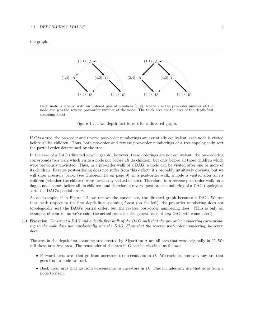
On the other hand, the terms ancestor , child , and descendant are always to be understood with referenceto a particular spanning forest D for G. So in particular, a node x may be an ancestor of another node ywith respect to one spanning forest for G, but not with respect to another. Figure 1.2 shows two differentwalks of a graph G. The edges of the depth-first spanning forest in each case are indicated by thick arcs in
1.1. DEPTH-FIRST WALKS 3
the graph.
A(3,1)
B(1,4) C(4,2)
D(2,5) E(5,3)
A(1,1)
B(2,4) C(4,2)
D(3,5) E(5,3)
Each node is labeled with an ordered pair of numbers (x, y), where x is the pre-order number of thenode and y is the reverse post-order number of the node. The thick arcs are the arcs of the depth-firstspanning forest.
Figure 1.2: Two depth-first forests for a directed graph.
If G is a tree, the pre-order and reverse post-order numberings are essentially equivalent; each node is visitedbefore all its children. Thus, both pre-order and reverse post-order numberings of a tree topologically sortthe partial order determined by the tree.
In the case of a DAG (directed acyclic graph), however, these orderings are not equivalent: the pre-orderingcorresponds to a walk which visits a node not before all its children, but only before all those children whichwere previously unvisited. Thus, in a pre-order walk of a DAG, a node can be visited after one or more ofits children. Reverse post-ordering does not suffer from this defect: it’s probably intuitively obvious, but wewill show precisely below (see Theorem 1.8 on page 9), in a post-order walk, a node is visited after all its
children (whether the children were previously visited or not). Therefore, in a reverse post-order walk on adag, a node comes before all its children, and therefore a reverse post-order numbering of a DAG topologicalsorts the DAG’s partial order.
As an example, if in Figure 1.2, we remove the curved arc, the directed graph becomes a DAG. We seethat, with respect to the first depth-first spanning forest (on the left), the pre-order numbering does not
topologically sort the DAG’s partial order, but the reverse post-order numbering does. (This is only an
example, of course—as we’ve said, the actual proof for the general case of any DAG will come later.)
1.1 Exercise Construct a DAG and a depth-first walk of the DAG such that the pre-order numbering correspond-ing to the walk does not topologically sort the DAG. Show that the reverse post-order numbering, however,does.
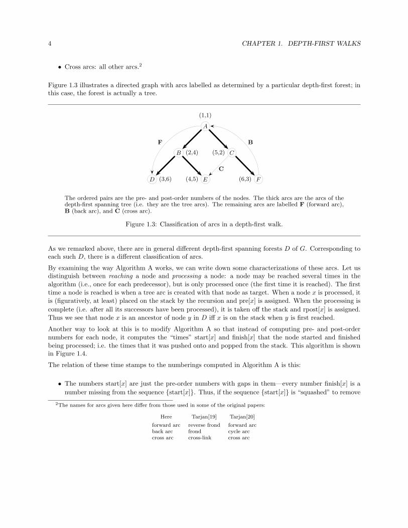
The arcs in the depth-first spanning tree created by Algorithm A are all arcs that were originally in G. Wecall these arcs tree arcs . The remainder of the arcs in G can be classified as follows:
• Forward arcs: arcs that go from ancestors to descendants in D. We exclude, however, any arc thatgoes from a node to itself.
• Back arcs: arcs that go from descendants to ancestors in D. This includes any arc that goes from anode to itself.
4 CHAPTER 1. DEPTH-FIRST WALKS
• Cross arcs: all other arcs.2
Figure 1.3 illustrates a directed graph with arcs labelled as determined by a particular depth-first forest; inthis case, the forest is actually a tree.
A
(1,1)
B (2,4) C(5,2)
D (3,6) E(4,5) F(6,3)
C
F B
The ordered pairs are the pre- and post-order numbers of the nodes. The thick arcs are the arcs of thedepth-first spanning tree (i.e. they are the tree arcs). The remaining arcs are labelled F (forward arc),B (back arc), and C (cross arc).
Figure 1.3: Classification of arcs in a depth-first walk.
As we remarked above, there are in general different depth-first spanning forests D of G. Corresponding toeach such D, there is a different classification of arcs.
By examining the way Algorithm A works, we can write down some characterizations of these arcs. Let usdistinguish between reaching a node and processing a node: a node may be reached several times in thealgorithm (i.e., once for each predecessor), but is only processed once (the first time it is reached). The firsttime a node is reached is when a tree arc is created with that node as target. When a node x is processed, itis (figuratively, at least) placed on the stack by the recursion and pre[x] is assigned. When the processing is
complete (i.e. after all its successors have been processed), it is taken off the stack and rpost[x] is assigned.Thus we see that node x is an ancestor of node y in D iff x is on the stack when y is first reached.
Another way to look at this is to modify Algorithm A so that instead of computing pre- and post-ordernumbers for each node, it computes the “times” start[x] and finish[x] that the node started and finishedbeing processed; i.e. the times that it was pushed onto and popped from the stack. This algorithm is shownin Figure 1.4.
The relation of these time stamps to the numberings computed in Algorithm A is this:
• The numbers start[x] are just the pre-order numbers with gaps in them—every number finish[x] is a
number missing from the sequence {start[x]}. Thus, if the sequence {start[x]} is “squashed” to remove
2The names for arcs given here differ from those used in some of the original papers:
Here Tarjan[19] Tarjan[20]
forward arc reverse frond forward arcback arc frond cycle arccross arc cross-link cross arc
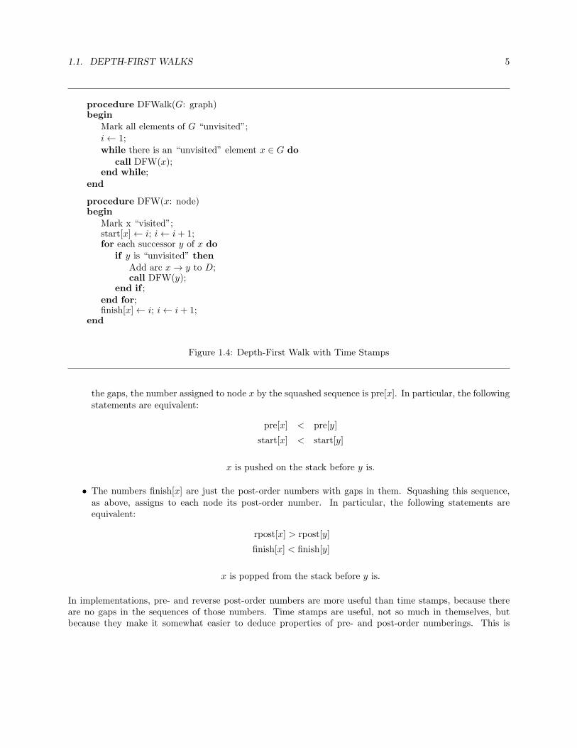
1.1. DEPTH-FIRST WALKS 5
procedure DFWalk(G: graph)begin
Mark all elements of G “unvisited”;
i← 1;
while there is an “unvisited” element x ∈ G docall DFW(x);
end while;
end
procedure DFW(x: node)begin
Mark x “visited”;start[x]← i; i← i+ 1;for each successor y of x do
if y is “unvisited” then
Add arc x→ y to D;call DFW(y);
end if ;
end for;finish[x]← i; i← i+ 1;
end
Figure 1.4: Depth-First Walk with Time Stamps
the gaps, the number assigned to node x by the squashed sequence is pre[x]. In particular, the followingstatements are equivalent:
pre[x] < pre[y]
start[x] < start[y]
x is pushed on the stack before y is.
• The numbers finish[x] are just the post-order numbers with gaps in them. Squashing this sequence,as above, assigns to each node its post-order number. In particular, the following statements areequivalent:
rpost[x] > rpost[y]
finish[x] < finish[y]
x is popped from the stack before y is.
In implementations, pre- and reverse post-order numbers are more useful than time stamps, because thereare no gaps in the sequences of those numbers. Time stamps are useful, not so much in themselves, butbecause they make it somewhat easier to deduce properties of pre- and post-order numberings. This is

6 CHAPTER 1. DEPTH-FIRST WALKS
because, in addition to the relations just noted, they satisfy two additional properties which we state in theform of two lemmas:
1.2 Lemma For each node x, start[x] < finish[x].
Proof. This just says that x is always pushed on the stack before it is popped off the stack.
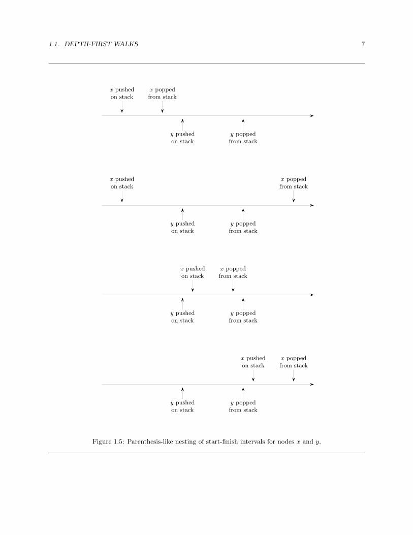
1.3 Lemma (Parenthesis Nesting Property) For any two nodes x and y, the start and finish numbers of x
and y nest as parentheses. That is, only the following relations are possible (see Figure 1.5):
start[x] < finish[x] < start[y] < finish[y]
start[x] < start[y] < finish[y] < finish[x]
start[y] < start[x] < finish[x] < finish[y]
start[y] < finish[y] < start[x] < finish[x]
Proof. If start[x] < start[y] < finish[x] then x is on the stack when y is first reached. Therefore theprocessing of y starts while x is on the stack, and so it also must finish while x is on the stack: we havestart[x] < start[y] < finish[y] < finish[x]. The case when start[y] < start[x] < finish[y] is handled in the sameway.
Another way to state the parenthesis nesting property is that given any two nodes x and y, the intervals[start[x], finish[x]] and [start[y], finish[y]] must be either nested or disjoint.
1.4 Lemma x is an ancestor of y iff both pre[x] < pre[y] and rpost[x] < rpost[y].
Proof. x is an ancestor of y iff x is first reached before y is and the processing of y is complete before theprocessing of x is. This in turn is true iff start[x] < start[y] < finish[y] < finish[x].
All four of the relations illustrated in Figure 1.5 are possible. However, when there is an arc in the graph Gfrom x to y, the last one can never occur. This is the content of the next theorem:
1.5 Theorem The following table characterizes the pre- and reverse post-order numberings of arcs x → y in adirected graph G with respect to a depth-first walk:
Tree Arc pre[x] < pre[y] rpost[x] < rpost[y]
Forward Arc pre[x] < pre[y] rpost[x] < rpost[y]
Back Arc pre[x] ≥ pre[y] rpost[x] ≥ rpost[y]
Cross Arc pre[x] > pre[y] rpost[x] < rpost[y]
Proof. The first three lines of the table follow from Lemma 1.4. As for the last line of the table, there aretwo possibilities:
• The processing of y began before the processing of x began. That is, start[y] < start[x]. Since y is not
an ancestor of x, then we must also have finish[y] < start[x](< finish[x]), and this is just the last lineof the table.
1.1. DEPTH-FIRST WALKS 7
x pushedon stack
x poppedfrom stack
y pushedon stack
y poppedfrom stack
x pushedon stack
x poppedfrom stack
y pushedon stack
y poppedfrom stack
x pushedon stack
x poppedfrom stack
y pushedon stack
y poppedfrom stack
x pushedon stack
x poppedfrom stack
y pushedon stack
y poppedfrom stack
Figure 1.5: Parenthesis-like nesting of start-finish intervals for nodes x and y.

8 CHAPTER 1. DEPTH-FIRST WALKS
• y was not reached before the processing of x began. But in this case, since y is a successor of x, ywill be reached while x is on the stack. That is, we have start[x] < start[y] < finish[x], and so y is adescendant of x, contradicting the assumption that x→ y is a cross arc.
Following Tarjan[19], we modify Algorithm A by initializing both the arrays pre[ ] and rpost[ ] to 0. So at
any point in the algorithm, pre[x] = 0 iff x has not yet been reached for the first time. (This does away with
the need to mark nodes as “visited”.) In addition, rpost[x] = 0 iff the processing of x is not finished. (It
might not even have started, but at any rate, it’s not finished.)
The modified algorithm, which we call Algorithm B (Figure 1.6), walks G and simultaneously constructs the
pre-ordering and reverse post-ordering of G, classifies all the arcs in G (thereby constructing D as well), and
computes the number of descendants ND[x] of each node x in the tree D. (Note: ND[x] is the number ofelements in the subtree of D which is rooted at x. This reflects the fact that conventionally, any node is adescendant of itself.)
1.6 Theorem Algorithm B generates a spanning forest D of G, computes the number of descendants in D ofeach node x, and correctly classifies arcs in G relative to D.
Proof. First, every node except the nodes x selected in the FOR loop is reached exactly once by a treearc. So the tree arcs form a forest of trees rooted at those nodes x.
By the construction in the algorithm, if x is a terminal node in D then ND[x] = 1, and otherwise
ND[x] = 1 +∑{ND[y] : x→ y is an arc in D}
which is what we mean by the number of descendants of x.
Theorem 1.5 then shows that the rest of the arcs are labelled correctly.
1.2 A Characterization of DAGS
Using these properties of arcs, we can characterize directed graphs which are DAGS:
1.7 Theorem If G is a directed graph, the following are equivalent:
1. G is a DAG.
2. There is a depth-first walk of G with no back arcs. (More precisely, there is a depth-first walk of G
with respect to which no arc in G is a back arc.)
3. No depth-first walk of G has back arcs. (More precisely, there is no arc in G which is a back arc with
respect to any depth-first walk of G.)
Proof. 1 =⇒ 3: Since there are no cycles in a DAG, there can be no back arcs with respect to any depth-firstwalk.
3 =⇒ 2: because 3 is stronger than 2.
2 =⇒ 1: By assumption, there is a depth-first walk of G with no back arcs. Let the pre-order and reversepost-order numbering of the nodes in G be determined by this walk. Now if G is not a DAG, then G containsa cycle. But then every edge x→ y in the cycle would satisfy rpost[x] < rpost[y], which is impossible.
1.2. A CHARACTERIZATION OF DAGS 9
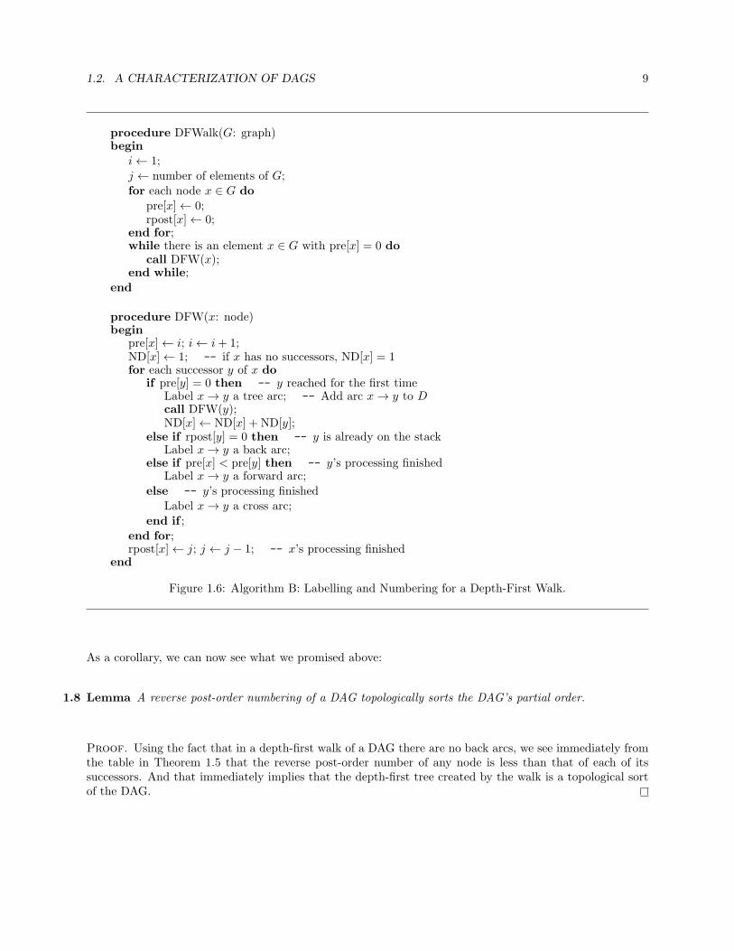
procedure DFWalk(G: graph)begin
i← 1;
j ← number of elements of G;
for each node x ∈ G dopre[x]← 0;rpost[x]← 0;
end for;while there is an element x ∈ G with pre[x] = 0 do
call DFW(x);end while;
end
procedure DFW(x: node)begin
pre[x]← i; i← i+ 1;ND[x]← 1; -- if x has no successors, ND[x] = 1for each successor y of x do
if pre[y] = 0 then -- y reached for the first timeLabel x→ y a tree arc; -- Add arc x→ y to Dcall DFW(y);ND[x]← ND[x] + ND[y];
else if rpost[y] = 0 then -- y is already on the stackLabel x→ y a back arc;
else if pre[x] < pre[y] then -- y’s processing finishedLabel x→ y a forward arc;
else -- y’s processing finished
Label x→ y a cross arc;end if ;
end for;rpost[x]← j; j ← j − 1; -- x’s processing finished
end
Figure 1.6: Algorithm B: Labelling and Numbering for a Depth-First Walk.
As a corollary, we can now see what we promised above:
1.8 Lemma A reverse post-order numbering of a DAG topologically sorts the DAG’s partial order.
Proof. Using the fact that in a depth-first walk of a DAG there are no back arcs, we see immediately fromthe table in Theorem 1.5 that the reverse post-order number of any node is less than that of each of itssuccessors. And that immediately implies that the depth-first tree created by the walk is a topological sortof the DAG.
10 CHAPTER 1. DEPTH-FIRST WALKS
1.3 A Characterization of Descendants
Again we let G be a directed graph with a depth-first walk which generates a spanning forest D by AlgorithmB. We will characterize descendants in D. (Actually, we could just start with a spanning forest D and a
depth-first walk of that forest, since the descendant relation is determined only by arcs in D.)
We already know by Lemma 1.4 that if z is a descendant of x, then pre[x] < pre[z] and rpost[x] < rpost[z].
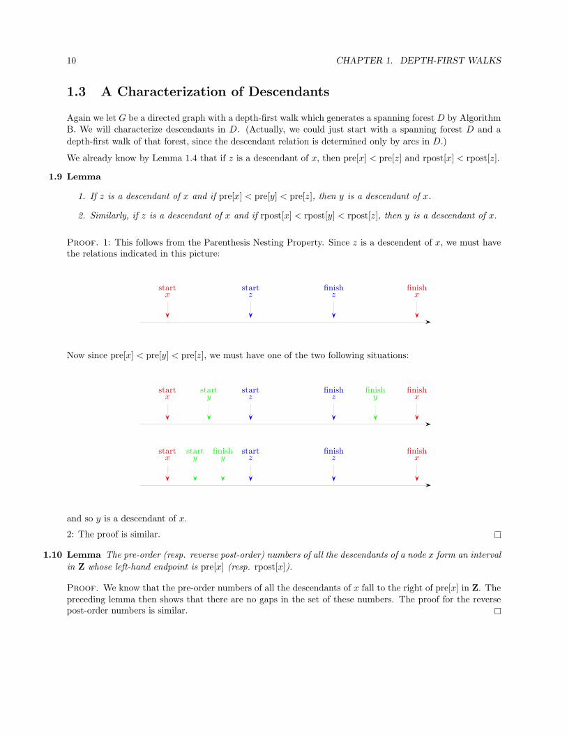
1.9 Lemma
1. If z is a descendant of x and if pre[x] < pre[y] < pre[z], then y is a descendant of x.
2. Similarly, if z is a descendant of x and if rpost[x] < rpost[y] < rpost[z], then y is a descendant of x.
Proof. 1: This follows from the Parenthesis Nesting Property. Since z is a descendent of x, we must havethe relations indicated in this picture:
startx
finishx
startz
finishz
Now since pre[x] < pre[y] < pre[z], we must have one of the two following situations:
startx
finishx
starty
finishy
startz
finishz
startx
finishx
starty
finishy
startz
finishz
and so y is a descendant of x.
2: The proof is similar.
1.10 Lemma The pre-order (resp. reverse post-order) numbers of all the descendants of a node x form an interval
in Z whose left-hand endpoint is pre[x] (resp. rpost[x]).
Proof. We know that the pre-order numbers of all the descendants of x fall to the right of pre[x] in Z. Thepreceding lemma then shows that there are no gaps in the set of these numbers. The proof for the reversepost-order numbers is similar.

1.4. THE PATH LEMMA 11
1.11 Theorem The following are equivalent:
1. x is an ancestor of y.
2. pre[x] < pre[y] and rpost[x] < rpost[y].
3. pre[x] < pre[y] < pre[x] + ND[x].
4. rpost[x] < rpost[y] < rpost[x] + ND[x].
Proof. 1 ⇐⇒ 2 is just Lemma 1.4. 1 ⇐⇒ 3 and 1 ⇐⇒ 4 by the preceding lemma.
1.4 The Path Lemma
1.12 Lemma If there is a path x = s0 → s1 → . . .→ sn = y such that pre[x] < pre[sj ] for 1 ≤ j ≤ n, then y is a
descendant of x.
Remarks 1. By the same token, every element of the path is a descendant of x.
2. The condition asserts that at the time that x is first reached, no element of the path from x to y has yetbeen reached.
Proof. We will show by induction on j that each element sj is a descendant of x. Of course this is true for
j = 0. Now say it is true for a particular value j; i.e. say we know that sj is a descendant of x. If j = n, of
course, we are done. Otherwise, we have to show that sj+1 is also a descendant of x. To do this, we look at
the arc sj → sj+1.
If the arc is a tree arc or a forward arc, then sj+1 is a descendent of sj , and we are done.
Otherwise, by Theorem 1.5, we have
pre[x] < pre[sj+1] < pre[sj ]
so again sj+1 is a descendant of x, by Lemma 1.9.
1.13 Lemma (Tarjan’s “Path Lemma”) If pre[x] < pre[y], then any path from x to y must contain a commonancestor of x and y.
Proof. This is an immediate corollary of Lemma 1.12: Let m be the node on the path such that pre[m] is
a minimum. By the Lemma, m is an ancestor of y. Further, either m = x (in which case m is trivially an
ancestor of x), or we have pre[m] < pre[x] < pre[y], so m is also an ancestor of x by Lemma 1.9.
Note that Lemma 1.12 also follows easily from Lemma 1.13.
1.5 An Application: Strongly Connected Components
In this section we present an efficient algorithm for computing the strongly connected components of anarbitrary directed graph G.
12 CHAPTER 1. DEPTH-FIRST WALKS
The reverse graph Gr of G is the graph with the same nodes as G but with each edge reversed (i.e. “pointing
in the opposite direction”). It is immediate that the strongly connected components of G are the same asthose of Gr.
1.14 Lemma If {Ti} is the spanning forest of trees produced by a depth-first traversal of G, then (the set of nodes
of) each strongly connected component of G is contained in (the set of nodes of) one of the Ti.
Remark Intuitively, once a depth-first walk reaches one node of a strongly connected component, it willreach all other nodes in that component in the same depth-first tree of the walk. The path lemma enablesus to give a quick proof of this fact:
Proof. If x and y are contained in the same strongly connected component of G, let us suppose withoutloss of generality that pre[x] < pre[y]. Since we know there is a path from x to y, some element u of thatpath is an ancestor of x and y. That is, x, y, and u must all belong to the same tree in the forest. Since xand y are arbitrary, each element in the strongly connected component must belong to that same tree.
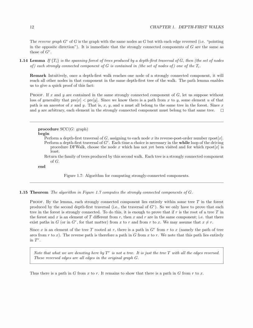
procedure SCC(G: graph)begin
Perform a depth-first traversal of G, assigning to each node x its reverse-post-order number rpost[x].Perform a depth-first traversal of Gr. Each time a choice is necessary in the while loop of the driving
procedure DFWalk, choose the node x which has not yet been visited and for which rpost[x] isleast.
Return the family of trees produced by this second walk. Each tree is a strongly connected componentof G.
end
Figure 1.7: Algorithm for computing strongly-connected components.
1.15 Theorem The algorithm in Figure 1.7 computes the strongly connected components of G.
Proof. By the lemma, each strongly connected component lies entirely within some tree T in the forestproduced by the second depth-first traversal (i.e., the traversal of Gr). So we only have to prove that eachtree in the forest is strongly connected. To do this, it is enough to prove that if r is the root of a tree T inthe forest and x is an element of T different from r, then x and r are in the same component; i.e. that thereexist paths in G (or in Gr, for that matter) from x to r and from r to x. We may assume that x 6= r.
Since x is an element of the tree T rooted at r, there is a path in Gr from r to x (namely the path of tree
arcs from r to x). The reverse path is therefore a path in G from x to r. We note that this path lies entirelyin T r.
Note that what we are denoting here by T r is not a tree. It is just the tree T with all the edges reversed.These reversed edges are all edges in the original graph G.
Thus there is a path in G from x to r. It remains to show that there is a path in G from r to x.
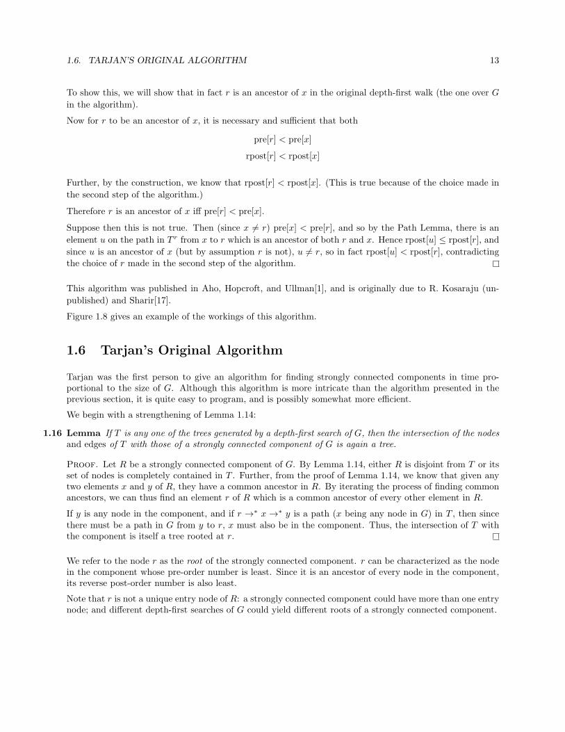
1.6. TARJAN’S ORIGINAL ALGORITHM 13
To show this, we will show that in fact r is an ancestor of x in the original depth-first walk (the one over G
in the algorithm).
Now for r to be an ancestor of x, it is necessary and sufficient that both
pre[r] < pre[x]
rpost[r] < rpost[x]
Further, by the construction, we know that rpost[r] < rpost[x]. (This is true because of the choice made in
the second step of the algorithm.)
Therefore r is an ancestor of x iff pre[r] < pre[x].
Suppose then this is not true. Then (since x 6= r) pre[x] < pre[r], and so by the Path Lemma, there is an
element u on the path in T r from x to r which is an ancestor of both r and x. Hence rpost[u] ≤ rpost[r], and
since u is an ancestor of x (but by assumption r is not), u 6= r, so in fact rpost[u] < rpost[r], contradictingthe choice of r made in the second step of the algorithm.
This algorithm was published in Aho, Hopcroft, and Ullman[1], and is originally due to R. Kosaraju (un-
published) and Sharir[17].
Figure 1.8 gives an example of the workings of this algorithm.
1.6 Tarjan’s Original Algorithm
Tarjan was the first person to give an algorithm for finding strongly connected components in time pro-portional to the size of G. Although this algorithm is more intricate than the algorithm presented in theprevious section, it is quite easy to program, and is possibly somewhat more efficient.
We begin with a strengthening of Lemma 1.14:
1.16 Lemma If T is any one of the trees generated by a depth-first search of G, then the intersection of the nodesand edges of T with those of a strongly connected component of G is again a tree.
Proof. Let R be a strongly connected component of G. By Lemma 1.14, either R is disjoint from T or itsset of nodes is completely contained in T . Further, from the proof of Lemma 1.14, we know that given anytwo elements x and y of R, they have a common ancestor in R. By iterating the process of finding commonancestors, we can thus find an element r of R which is a common ancestor of every other element in R.
If y is any node in the component, and if r →∗ x →∗ y is a path (x being any node in G) in T , then sincethere must be a path in G from y to r, x must also be in the component. Thus, the intersection of T withthe component is itself a tree rooted at r.
We refer to the node r as the root of the strongly connected component. r can be characterized as the nodein the component whose pre-order number is least. Since it is an ancestor of every node in the component,its reverse post-order number is also least.
Note that r is not a unique entry node of R: a strongly connected component could have more than one entrynode; and different depth-first searches of G could yield different roots of a strongly connected component.

14 CHAPTER 1. DEPTH-FIRST WALKS
(1,2)
(2,3)
(3,4)
(4,6)
(5,7)
(8,5)
(7,9)
(6,8)
(9,1)
A depth-first walk in a directed graph. The ordered pairs by each nodeshow the pre-order and reverse post-order numbers determined by the walk.
1
2
3
Figure 1.8: The reverse graph, showing the strongly connected components as found by the algorithm ofSection 1.5. The numbers show the order in which the components are discovered.
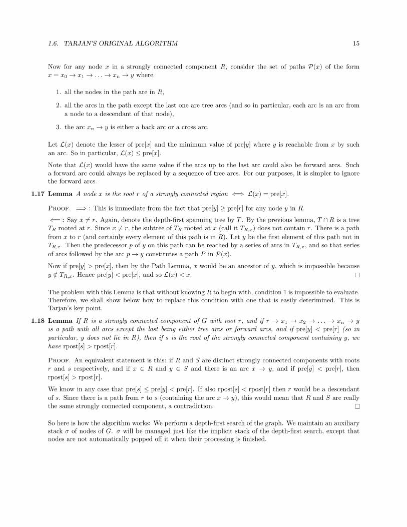
1.6. TARJAN’S ORIGINAL ALGORITHM 15
Now for any node x in a strongly connected component R, consider the set of paths P(x) of the formx = x0 → x1 → . . .→ xn → y where
1. all the nodes in the path are in R,
2. all the arcs in the path except the last one are tree arcs (and so in particular, each arc is an arc from
a node to a descendant of that node),
3. the arc xn → y is either a back arc or a cross arc.
Let L(x) denote the lesser of pre[x] and the minimum value of pre[y] where y is reachable from x by such
an arc. So in particular, L(x) ≤ pre[x].
Note that L(x) would have the same value if the arcs up to the last arc could also be forward arcs. Sucha forward arc could always be replaced by a sequence of tree arcs. For our purposes, it is simpler to ignorethe forward arcs.
1.17 Lemma A node x is the root r of a strongly connected region ⇐⇒ L(x) = pre[x].
Proof. =⇒ : This is immediate from the fact that pre[y] ≥ pre[r] for any node y in R.
⇐= : Say x 6= r. Again, denote the depth-first spanning tree by T . By the previous lemma, T ∩R is a treeTR rooted at r. Since x 6= r, the subtree of TR rooted at x (call it TR,x) does not contain r. There is a path
from x to r (and certainly every element of this path is in R). Let y be the first element of this path not inTR,x. Then the predecessor p of y on this path can be reached by a series of arcs in TR,x, and so that series
of arcs followed by the arc p→ y constitutes a path P in P(x).
Now if pre[y] > pre[x], then by the Path Lemma, x would be an ancestor of y, which is impossible because
y /∈ TR,x. Hence pre[y] < pre[x], and so L(x) < x.
The problem with this Lemma is that without knowing R to begin with, condition 1 is impossible to evaluate.Therefore, we shall show below how to replace this condition with one that is easily deterimined. This isTarjan’s key point.
1.18 Lemma If R is a strongly connected component of G with root r, and if r → x1 → x2 → . . . → xn → yis a path with all arcs except the last being either tree arcs or forward arcs, and if pre[y] < pre[r] (so in
particular, y does not lie in R), then if s is the root of the strongly connected component containing y, we
have rpost[s] > rpost[r].
Proof. An equivalent statement is this: if R and S are distinct strongly connected components with rootsr and s respectively, and if x ∈ R and y ∈ S and there is an arc x → y, and if pre[y] < pre[r], then
rpost[s] > rpost[r].
We know in any case that pre[s] ≤ pre[y] < pre[r]. If also rpost[s] < rpost[r] then r would be a descendant
of s. Since there is a path from r to s (containing the arc x→ y), this would mean that R and S are reallythe same strongly connected component, a contradiction.
So here is how the algorithm works: We perform a depth-first search of the graph. We maintain an auxiliarystack σ of nodes of G. σ will be managed just like the implicit stack of the depth-first search, except thatnodes are not automatically popped off it when their processing is finished.

16 CHAPTER 1. DEPTH-FIRST WALKS
To be precise, σ is managed as follows: As each node is first reached, it is pushed on σ. (That is, the
nodes of G are pushed on σ in pre-order.) Thus the descendants of each node lie above the node on σ.In particular, the roots of the strongly connected components of G will eventually be on σ with the otherelements of their component above them. When the processing (i.e. in the depth-first walk) for a root r is
finished, we pop every element in the stack down to and including r. (For this to happen, of course, we have
to be able to identify the nodes which are roots of strongly connected regions. We deal with this below.)No other elements of other strongly connected regions can be among the elements popped. This is becauseif y were such an element, it would have been placed on the stack after r was first reached and before theprocessing of r was finished, and so would be a descendant of r. So by the preceding lemma, the root s ofthe component of y would also be a descendant of r, and so would have been placed above r on the stack.Since its processing would have been finished before r’s processing, s and all nodes higher than it on thestack, including y, would already have been popped off the stack before we pop r.
As noted above, for this algorithm to work, we have to be able to identify the roots of the strongly connectedregions. Using the stack σ, we can do this as follows: for each node x being processed, compute the attributeL[x] (L is the replacement for L above), whose value is defined to be the lesser of pre[x] and the minimum
of pre[y] taken over all y such that there is a path x = x0 → x1 → . . .→ xn → y where
1. Each arc up to xn is a tree arc.
2. The arc xn → y is a back arc or a cross arc.
3. y is on σ at some point during the processing of x.
Here condition 3 substitutes for the previous condition 1.
The same argument as in Lemma 1.17 shows that if x is not a root, then L[x] < pre[x].
On the other hand, let r be a root, and let y be that node for which pre[y] = L(r). Now the only way
we could have L[r] < pre[r] is if the y belonged to a strongly connected component with root s such that
rpost[s] > rpost[r]. Since we also have pre[s] ≤ pre[y] = L(r) < pre[r], we have
start[s] < start[r]
finish[s] < finish[r]
and so by the parenthesis nesting property, finish[s] < start[r]; i.e., the processing of s is finished before the
processing of r starts, which means that s (and hence y) is not on the stack at any time during the processing
of r. Hence L[r] = pre[r].
Thus in the algorithm, we compute L[x] for each node as it is processed. When the processing of the node is
finished, if L[x] = pre[x], it is known to be a root, and it and all elements above it on the stack are poppedand constitute a strongly connected component.
The complete algorithm is shown in Figure 1.9. Figure 1.10 shows the order in which the strongly connectedcomponents of the graph in Figure 1.8 are discovered, with the same depth-first walk as in that figure.

1.6. TARJAN’S ORIGINAL ALGORITHM 17
function SCCwalk(G: graph): set of sets of nodesσ: stack of nodes;SetOfComponents : set of sets of nodes;
begin
Initialize the stack σ to be empty;SetOfComponents← ∅;i← 1;
for each node x ∈ G doL[g]← 0;pre[x]← 0;
end for;while there is an element x ∈ G with pre[x] = 0 do
call SCC(x);end while;
return SetOfComponents ;end
procedure SCC(x: node)begin
pre[x]← i; i← i+ 1;L[x]← pre[x];push x onto σ;
for each successor y of x doif pre[y] = 0 then -- x→ y is a tree arc.
call SCC(y);if L[y] < L[x] then
L[x]← L[y];end if ;
else if pre[x] < pre[y] -- x→ y is a forward arc.Do nothing;
else -- x→ y is a back or cross arc.if (y is on σ) and (pre[y] < L[x]) then
L[x]← pre[y];end if ;
end if ;
end for;if L[x] = pre[x] then
C ← ∅;repeat
pop z from σ;Add z to C;
until z = x;
end if ;Add C to SetOfComponents ;
end
Figure 1.9: Tarjan’s original algorithm for finding strongly connected components.

18 CHAPTER 1. DEPTH-FIRST WALKS
3
2
1
Figure 1.10: The same directed graph as in Figure 1.8. Given the same depth-first walk of this graph,this figure shows the order in which the, showing the strongly connected components are discovered by thealgorithm of Section 1.6.
Chapter 2
Flow Graphs
2.1 Flow Graphs
A flow graph is a finite directed graph G together with a distinguished element s (“start”, the “initial
element”) such that every element in G is reachable by a path from s. Henceforth, G will always be a flow
graph with initial element s. As a notational convenience, we may sometimes write 〈G, s〉 to denote this flowgraph.
A flow graph must have at least one node (i.e., s). A flow graph with only one node is called the trivial flowgraph.
If P is a path x0 → x1 → . . . → xn in G, we call the nodes {x1, . . . , xn−1} the interior points of the path.A loop or cycle is a path which starts and ends at the same node. A self-loop is a loop of the form x → x.We say that the path P is simple or cycle-free iff all the nodes {xj : 0 ≤ j ≤ n} in it are distinct.
If there is a path from x to y, then there is a simple path from x to y. (This is a simple proof by inductionon the number of elements in the path. If the path is not simple, then there must be a cycle in it; removingthe cycle is the inductive step.)
Most of our conventional usage for directed graphs applies in particular to flow graphs:
• If x→ y is an arc in a flow graph, we say that x is a predecessor of y, and that y is a successor of x.
• The terms ancestor , child , and descendant have different meanings: they always refer to relationswithin a tree (e.g. a dominator tree, or the spanning tree of a flow graph).
• To be precise, we should really denote a flow graph by 〈G,A, s〉, where A is the set of arcs (i.e. edges)in the graph. However, we will generally omit reference to A.
• Similarly, a sub graph of a flow graph 〈G,A, s〉 should really be denoted 〈H,E〉, where E is a collectionof edges in A connecting elements of H. However, in general we denote a sub graph of G simply byH. We will make the convention that the edges in the sub graph consist of all edges in the flow graphconnecting members of H.
19

20 CHAPTER 2. FLOW GRAPHS
• The one exception to this convention is when the sub graph H of G is a tree or a forest of trees. In thiscase, the edges of H are understood to be only the tree edges, ignoring any other edges of G betweenmembers of H.
2.2 Dominators
If x and y are two elements in a flow graph G, then x dominates y (x is a dominator of y) iff every path
from s to y includes x. If x dominates y, we will write x≫y. For example, in Figure 2.1 (modified from a
graph in Tarjan[19]), C dominates J , but C does not dominate I.
S
C B
F G E A
I J H D
K
Figure 2.1: A flow graph in which we wish to find dominators.
In particular, if x is any element of G, then x dominates itself, and s dominates x. If x≫y and x 6= y, we saythat x strongly dominates y, and write s≫ y. The negation of x≫y is x 6≫ y, and the negation of x≫ y isx 6≫ y.
2.1 Lemma The dominance relation is a partial order on G. That is, for all x, y, and z in G,
1. x≫x.
2. If x≫y and y≫x, then x = y.
3. If x≫y and y≫z, then x≫z.
Proof. 1 and 3 are obvious.
To prove 2, let P be a simple path from s to y. Then P must include x. But then the initial part of thepath from s to x must itself include y. So unless x = y, the path includes y in two different positions, andis not simple, a contradiction.
2.2 Lemma If x and y both dominate z then either x≫y or y≫x.

2.2. DOMINATORS 21
Proof. Let P be a simple path from s to z. P must contain both x and y. If y occurs after x, then x≫y,
for if not, there would be a path P ′ from s to y which did not include x. Replacing that part of P from sto y with P ′ yields a path from s to z not including x, a contradiction. Similarly, if x occurs after y in P ,then y≫x.
Thus, the set of dominators of a node x is linearly ordered. In particular, every element x of G except shas an immediate dominator ; i.e. an element y such that y ≫ x and if z ≫ x then z≫y. We denote the
immediate dominator of x by idom(x).
Now let us define a graph T on the elements of G as follows: there is an arc from x to y iff x is the immediatedominator of y.
2.3 Lemma T is a tree rooted at s.
Proof. s has no predecessors in T . (s has no dominators other than s itself.)
The in-degree of each element except s is 1. (There is only 1 arc leading to any x 6= s; namely the arc from
its immediate dominator.)
Every element in G is reachable from s in T . (s dominates every element in G, and following the immediate
dominator chain of any element x back from x leads to s.)
T is called the dominator tree of G. Figure 2.2 shows the dominator tree for the flow graph of Figure 2.1.
S
I K C B A
F G E D
J H
Figure 2.2: The dominator tree for the flow graph of Figure 2.1.
There are some relations between the arcs in 〈G, s〉 and the arcs in its dominator tree T . An arc in T may
correspond to an arc in 〈G, s〉, or it may not. (For instance, the arc S → I in the dominator tree in Figure 2.2
does not correspond to an arc in the flow graph in Figure 2.1.) In general, an arc in 〈G, s〉 falls into one ofthe following three categories:
1. Arcs x → y where x is an ancestor of y in T (i.e. x dominates y). In this case, x must in fact be the
parent of y in T (i.e. x = idom(y)), since otherwise there would be a path from s to x and then to
y which avoided idom(y) in T , a contradiction. (As we have seen, however, not every arc in T has to
come from an arc in 〈G, s〉.)

22 CHAPTER 2. FLOW GRAPHS
2. Arcs x → y where y is an ancestor of x in T (i.e. where y dominates x . (These we may call “back
arcs”; cf. the beginning of the proof of Theorem 3.25.)
3. All other arcs x → y. y cannot be s, since then y≫x, which was handled by the previous case.
Therefore, y has an immediate dominator z = idom(y). Further, z must be an ancestor of x in T (i.e.
z = idom(y)≫x), since otherwise there would be a path from s to x, and then to y, which avoided z,again a contradiction.
Figure 2.1 contains examples of each of these three types of arcs. In any case, we see that if x→ y is an arcin G then either y is an ancestor of x in T or the parent of y in T is an ancestor of x in T . That is, either ydominates x or the immediate dominator of y dominates x. We will give a name to this result:
2.4 Lemma (Dominator Lemma) If x→ y is an arc in a flow graph G, then either
1. y≫x, or
2. y 6= s and idom(y)≫x.
Equivalently, either y = s or idom(y)≫x.
2.3 Depth-First Spanning Trees
We will perform depth-first walks of flow graphs. All such walks will start at s; hence the spanning foreststhey generate will all be trees. Algorithm B of Chapter 1 (Figure 1.6) thus can be rewritten a little moresimply as shown in Figure 2.3.
2.5 Theorem The pre-order and reverse post-order numberings corresponding to any depth-first walk of a flowgraph G each topologically sort the dominance partial ordering in G.
Proof. If x dominates y, then x must be an ancestor of y in any depth-first walk of G. Hence pre[x] < pre[y]
and rpost[x] < rpost[y] by the lemma.
The study of flow graphs inevitably revolves about the study of loops—if there are no loops in a flow graph,the graph is a DAG, and in some sense the flow of control in the computer program it represents is trivial.So one of the main problems that has to be faced is how to get a handle on the looping structure of a flowgraph. The simplest idea is undoubtedly to look at strongly connected subgraphs of the flow graph. In fact,it is evident that every flow graph can be uniquely decomposed into maximal strongly connected subgraphs.The problem with this is twofold:
1. If the graph is a DAG, every node in the graph is a separate maximal strongly connected subgraph.This is too much detail—we really don’t care about all those nodes individually.
2. If the program contains a triply nested loop, for instance, all three of those loops will be contained inthe same maximal strongly connected subgraph. This is too little detail. We want the decompositionto reflect the structure of loop inclusion.
We will see in chapter 3 how we can expose the looping structure of a flow graph by means of a decompositioninto intervals.
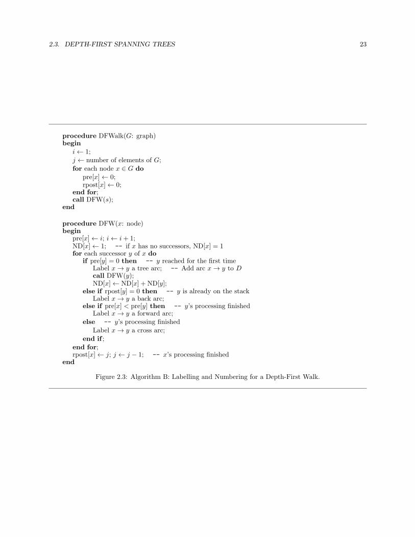
2.3. DEPTH-FIRST SPANNING TREES 23
procedure DFWalk(G: graph)begin
i← 1;
j ← number of elements of G;for each node x ∈ G do
pre[x]← 0;rpost[x]← 0;
end for;call DFW(s);
end
procedure DFW(x: node)begin
pre[x]← i; i← i+ 1;ND[x]← 1; -- if x has no successors, ND[x] = 1for each successor y of x do
if pre[y] = 0 then -- y reached for the first timeLabel x→ y a tree arc; -- Add arc x→ y to Dcall DFW(y);ND[x]← ND[x] + ND[y];
else if rpost[y] = 0 then -- y is already on the stackLabel x→ y a back arc;
else if pre[x] < pre[y] then -- y’s processing finishedLabel x→ y a forward arc;
else -- y’s processing finishedLabel x→ y a cross arc;
end if ;
end for;rpost[x]← j; j ← j − 1; -- x’s processing finished
end
Figure 2.3: Algorithm B: Labelling and Numbering for a Depth-First Walk.

Chapter 3
Reducible Flow Graphs
The definitions that follow are all motivated by the goal of finding intrinsic characterizations of single-entryloops; that is, loops that can be entered at only one flow graph node. Such loops can of course be nested—programmers do this all the time. We need to find a way of representing this nesting in a way that can beanalyzed efficiently.
3.1 Intervals
If H is a subset of nodes of a flow graph 〈G, s〉, then an element h of H is called an entry node of H iff either
1. h = s; or
2. there is an edge x→ h in G with x /∈ H.
A region in a flow graph is a sub graph H with a unique entry node h.
In particular, a region is a sub flow graph. We can write 〈H,h〉 to denote a region with entry h. We notethat since H has a unique entry node, if s ∈ H, we must have s = h. The term “header” is also used todescribe an entry node of a region.
A pre-interval in a flow graph is a region 〈H,h〉 such that every cycle in H includes h. That is, a pre-intervalin a flow graph is a sub graph H satisfying the following properties:
1. H has a unique entry node h.
2. Every cycle in H includes h.
An interval in a flow graph is a maximal pre-interval.1
3.1 Lemma Every element in a region 〈H,h〉 is reachable from h by a path in H.
1In the literature, no distinction is customarily made between an interval and what here is called a pre-interval, althoughsometimes an interval is referred to as a “maximal interval”. I have introduced the term pre-interval to make the distinctionexplicit. Pre-intervals are useful in proofs and in understanding the algorithms, but intervals are the objects of real interest.
24

3.1. INTERVALS 25
Proof. If x is any element of H, then since 〈G, s〉 is a flow graph, there is a path
P : s = x0 → x1 → x2 → . . .→ xn = x
Let xj−1 be the last element of this path not in H. Then since xj−1 → xj is an arc in G, xj is an entry node
of H and so must must equal h. Thus the path
xj → . . .→ xn = x
is a path in H from h to x.
3.2 Lemma If 〈H,h〉 is a region and x ∈ H, any simple path from h to x lies entirely within H.
Proof. If the path h = x0 → x1 → . . .→ xn = x does not lie entirely within H, then as in the proof of theprevious lemma, one of the points xj with j ≥ 2 is an entry node of H, and hence must be h. But then the
path is not simple.
3.3 Lemma If 〈H,h〉 is a region, then h dominates (in G) every other node in H.
Proof. If s ∈ H, then h = s, and so h dominates every element in G and so also in H.
Otherwise, there is a path from s to some node x in H which avoids h and which is not entirely contained inH. Let y be the last element on this path which is not in H, and let z be the next element on this path (so
z ∈ H; z might be x, in particular). Then as before, z is an entry node of H but z 6= h, a contradiction.
3.4 Theorem For each element h ∈ G, there is a region R(h) with header h which includes all other regions
with header h. R(h) consists of all elements of G which are dominated by h.
Remark The region is not a “maximal region” unless h = s; in fact, the only maximal region is 〈G, s〉 itself.But the region is maximal among all regions with header h.
Proof. Let H denote the family of regions with header h. Since {h} ∈ H, H 6= ∅. The union of any two
members of H is in H. But then since H is finite, the union of all the members of H is in H. Thus R(h)exists.
Let H = {x : h≫x}. By Lemma 3.3, R(h) ⊂ H.
To prove the converse inclusion, we will show thatH is a region with header h—this will show thatH ⊂ R(h).
If H is not such a region, then it has an entry node x different from h. Therefore there is an arc y → xwith y /∈ H. Since then y is not dominated by h, there is a path P from s to y which avoids h. But thenappending the arc y → x to the end of P yields a path from s to x which avoids h, a contradiction, becauseh dominates x. Thus H has h as its unique entry node, and is therefore a region, and so H ⊂ R(h).
3.5 Lemma A region is a convex subset of the dominator tree. That is, if 〈H,h〉 is a region, if x and y are inH, and if there is an element m ∈ G such that x≫m≫y, then m ∈ H.
Proof. If P is a simple path from s to y, then since h≫x, that part of P which starts at h is a simple pathfrom h to y which includes x and m. By Lemma 3.2, it lies entirely within H, so m ∈ H.
Remark Not every convex subset of the dominator tree is a region, however. For instance, the union of twodisjoint subtrees of the dominator tree is not a region.

26 CHAPTER 3. REDUCIBLE FLOW GRAPHS
3.6 Lemma If 〈H,h〉 and 〈K, k〉 are regions with a non-empty intersection, then either k ∈ H or h ∈ K. If
k ∈ H, then 〈H ∪K,h〉 is a region.
Proof. There must be a node x ∈ H ∩ K. Since h and k both dominate x, either h dominates k or kdominates h. Say h dominates k. Then by Lemma 3.4, k ∈ H. But then H ∪ K must be a region withheader h, for any path entering H ∪K either enters H (at h) or K (at k). But since k ∈ H, to reach k itmust first enter H at h.
3.7 Lemma If 〈H,h〉 and 〈K, k〉 are pre-intervals with a non-empty intersection, then either k ∈ H or h ∈ K.
If k ∈ H, then 〈H ∪K,h〉 is a pre-interval.
Proof. By the previous lemma, we already know that either k ∈ H or h ∈ K and that H ∪K is a region.Without loss of generality, let us assume that k ∈ H. We will show that 〈H ∪K,h〉 is a pre-interval.
Let C = {x0 → x1 → . . .→ xn = x0} be a cycle in H ∪K. If C ⊂ H, then C must include h. Otherwise,there is a node xj ∈ K −H, and there are two possibilities:
Case I: C ⊂ K. Then C includes k, which is in H, and so C enters H (since xj /∈ H), so C must enter H
at h; i.e. h ∈ C.
Case II: C 6⊂ K. Again, C must re-enter H (since it is not completely contained in K), so it must containh.
So in any case, h ∈ C, and so 〈H ∪K,h〉 is a pre-interval.
3.8 Theorem For each element h ∈ G, there is a pre-interval with header h which includes all other pre-intervalswith header h.
Remark The pre-interval is not necessarily a maximal pre-interval (i.e. is not necessarily an interval). Butthe pre-interval is maximal among all pre-intervals with header h.
Proof. As in the proof of Lemma 3.4, let H denote the family of pre-interals with header h. Since {h} ∈ H,
H 6= ∅. Lemma 3.7 shows that the union of any two members of H is in H. But then since H is finite, theunion of all members of H is in H.
3.9 Theorem If 〈H,h〉 and 〈K, k〉 are intervals in the flow graph 〈G, s〉, then they are either identical or disjoint.
Proof. If H and K are not disjoint, then by Lemma 3.7, H ∪K is a pre-interval. But then by maximality,H = H ∪K = K.
3.10 Theorem G can be uniquely partitioned into (disjoint) intervals.
Proof. Any single node in G by itself constitutes a pre-interval. Hence every node in G lies in some interval.That interval is unique by the previous theorem, and the set of all these intervals is disjoint by the theorem.
This last theorem is an essential and key fact concerning intervals.
3.2. ALGORITHMS FOR CONSTRUCTING INTERVALS 27
function MakePI(h: node)begin
A← {h}; -- initializewhile there exists a node m 6= s all of whose predecessors are in A do
A← A ∪ {m};end while;return A;
end
Figure 3.1: Algorithm C
Compute the Largest Pre-Interval with Header h
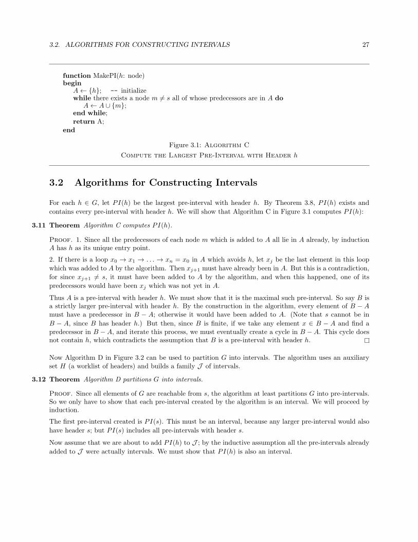
3.2 Algorithms for Constructing Intervals
For each h ∈ G, let PI(h) be the largest pre-interval with header h. By Theorem 3.8, PI(h) exists and
contains every pre-interval with header h. We will show that Algorithm C in Figure 3.1 computes PI(h):
3.11 Theorem Algorithm C computes PI(h).
Proof. 1. Since all the predecessors of each node m which is added to A all lie in A already, by inductionA has h as its unique entry point.
2. If there is a loop x0 → x1 → . . . → xn = x0 in A which avoids h, let xj be the last element in this loop
which was added to A by the algorithm. Then xj+1 must have already been in A. But this is a contradiction,
for since xj+1 6= s, it must have been added to A by the algorithm, and when this happened, one of its
predecessors would have been xj which was not yet in A.
Thus A is a pre-interval with header h. We must show that it is the maximal such pre-interval. So say B isa strictly larger pre-interval with header h. By the construction in the algorithm, every element of B − Amust have a predecessor in B − A; otherwise it would have been added to A. (Note that s cannot be in
B − A, since B has header h.) But then, since B is finite, if we take any element x ∈ B − A and find apredecessor in B −A, and iterate this process, we must eventually create a cycle in B −A. This cycle doesnot contain h, which contradicts the assumption that B is a pre-interval with header h.
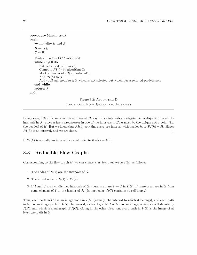
Now Algorithm D in Figure 3.2 can be used to partition G into intervals. The algorithm uses an auxiliaryset H (a worklist of headers) and builds a family J of intervals.
3.12 Theorem Algorithm D partitions G into intervals.
Proof. Since all elements of G are reachable from s, the algorithm at least partitions G into pre-intervals.So we only have to show that each pre-interval created by the algorithm is an interval. We will proceed byinduction.
The first pre-interval created is PI(s). This must be an interval, because any larger pre-interval would also
have header s; but PI(s) includes all pre-intervals with header s.
Now assume that we are about to add PI(h) to J ; by the inductive assumption all the pre-intervals already
added to J were actually intervals. We must show that PI(h) is also an interval.
28 CHAPTER 3. REDUCIBLE FLOW GRAPHS
procedure MakeIntervalsbegin
-- Initialize H and J :
H ← {s};J ← ∅;
Mark all nodes of G “unselected”.while H 6= ∅ do
Extract a node h from H;Compute PI(h) by algorithm C;Mark all nodes of PI(h) “selected”;Add PI(h) to J ;Add to H any node m ∈ G which is not selected but which has a selected predecessor;
end while;
return J ;end
Figure 3.2: Algorithm D
Partition a Flow Graph into Intervals
In any case, PI(h) is contained in an interval H, say. Since intervals are disjoint, H is disjoint from all the
intervals in J . Since h has a predecessor in one of the intervals in J , h must be the unique entry point (i.e.
the header) of H. But we know that PI(h) contains every pre-interval with header h, so PI(h) = H. Hence
PI(h) is an interval, and we are done.
If PI(h) is actually an interval, we shall refer to it also as I(h).
3.3 Reducible Flow Graphs
Corresponding to the flow graph G, we can create a derived flow graph I(G) as follows:
1. The nodes of I(G) are the intervals of G.
2. The initial node of I(G) is PI(s).
3. If I and J are two distinct intervals of G, there is an arc I → J in I(G) iff there is an arc in G from
some element of I to the header of J . (In particular, I(G) contains no self-loops.)
Thus, each node in G has an image node in I(G) (namely, the interval to which it belongs), and each path
in G has an image path in I(G). In general, each subgraph H of G has an image, which we will denote by
I(H), and which is a subgraph of I(G). Going in the other direction, every path in I(G) is the image of atleast one path in G.
3.3. REDUCIBLE FLOW GRAPHS 29
Note that the image of a simple path may not be simple. (A path can start in an interval but not at itsheader, leave that interval, and end by reentering the interval at its header. The path could be simple butthe image would not be.)
On the other hand, every path in I(G) is the image of a path in G, and a simple path in I(G) can be takento be the image of a simple path in G.
Now this process can be repeated: If we set G0 = G and for all j > 0 we set Gj = I(Gj−1), then the sequence
G0, G1, . . . is called the derived sequence for G.
The number of elements of I(Gj) is always ≤ the number of elements of Gj . Further, I(Gj) has the same
number of elements as Gj iff each element of Gj constitutes an interval of Gj , in which case I(Gj) = Gj .
Thus, after a finite number of terms, each term of the derived sequence is a fixed flow graph I(G) called the
limit flow graph of G. Every node of I(G) is an interval.
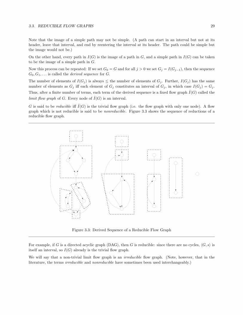
G is said to be reducible iff I(G) is the trivial flow graph (i.e. the flow graph with only one node). A flowgraph which is not reducible is said to be nonreducible. Figure 3.3 shows the sequence of reductions of areducible flow graph.
Figure 3.3: Derived Sequence of a Reducible Flow Graph
For example, if G is a directed acyclic graph (DAG), then G is reducible: since there are no cycles, 〈G, s〉 is
itself an interval, so I(G) already is the trivial flow graph.
We will say that a non-trivial limit flow graph is an irreducible flow graph. (Note, however, that in the
literature, the terms irreducible and nonreducible have sometimes been used interchangeably.)

30 CHAPTER 3. REDUCIBLE FLOW GRAPHS
Flow graphs which are generated by programs written in languages with structured flow of control statementssuch as if-then-else constructions and while loops but no goto statements are automatically reducible. Andin fact, it has been observed that competent programmers who do use goto statements virtually alwaysproduce code which leads to reducible flow graphs anyway. So nonreducible flow graphs really are in somesense pathological.
The concept of reducibility seems to be an intrinsically important one, as there are many striking character-izations of reducible flow graphs, as we will see below. Right now, we will prove a useful result relating thederived sequence to the dominance partial order:
3.13 Lemma If 〈H,h〉 and 〈K, k〉 are intervals in G and if x ∈ K, the following are equivalent:
1. H≫K in I(G).
2. h≫k in G.
3. h≫x in G.
Proof. 1 =⇒ 3: Otherwise, there would be a path from s to x which avoids h. But then this path cannotinclude any member of H, and so its image in I(G) avoids H; hence H does not dominate K in I(G).
3 =⇒ 2: Otherwise there would be a path from s to k not including h. Adjoining to this path the path inK from k to x gives a path from s to x not including h, a contradiction.
2 =⇒ 1: Any path from s to k must go through h, which means that any path in I(G) from I(s) to K must
go through H, so H≫K in I(G).
3.14 Theorem If x→ y is an arc in G, and if the images of x and y in an element Gj of the derived sequence
of G are xj and yj respectively and if xj 6= yj, then y≫x ⇐⇒ yj≫xj.
Proof. Let us say the images of x and y in the elements Gk of the derived sequence of G are xk and ykrespectively.
Since xj 6= yj , we must have yk 6= xk for 0 ≤ k ≤ j. Therefore the arc x → y has an image arc xk → yk in
Gk for 0 ≤ k ≤ j. For 0 ≤ k < j, xk and yk cannot be in the same interval of Gk, and hence yk must bean interval header in Gk. (This is where we use the fact that x→ y is an arc.) Hence applying Lemma 3.13repeatedly, we get
y≫x ⇐⇒ y1≫x1 ⇐⇒ . . . ⇐⇒ yj≫xj .
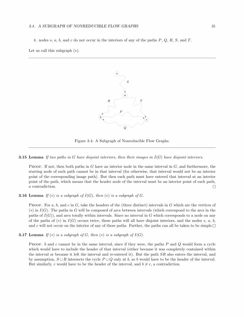
3.4 A Subgraph of Nonreducible Flow Graphs
We will show that a flow graph is nonreducible iff it contains a subgraph of the form in Figure 3.4, where
1. the paths P , Q, R, S, and T are all simple.
2. the paths P , Q, R, S, and T have pairwise disjoint interiors.
3. nodes s, a, b, and c are distinct, unless a = s, in which case there is no path S in the subgraph.
3.4. A SUBGRAPH OF NONREDUCIBLE FLOW GRAPHS 31
4. nodes s, a, b, and c do not occur in the interiors of any of the paths P , Q, R, S, and T .
Let us call this subgraph (∗).
s
a
bc
S
R T
P
Q
Figure 3.4: A Subgraph of Nonreducible Flow Graphs.
3.15 Lemma If two paths in G have disjoint interiors, then their images in I(G) have disjoint interiors.
Proof. If not, then both paths in G have an interior node in the same interval in G, and furthermore, thestarting node of each path cannot be in that interval (for otherwise, that interval would not be an interior
point of the corresponding image path). But then each path must have entered that interval at an interiorpoint of the path, which means that the header node of the interval must be an interior point of each path,a contradiction.
3.16 Lemma If (∗) is a subgraph of I(G), then (∗) is a subgraph of G.
Proof. For a, b, and c in G, take the headers of the (three distinct) intervals in G which are the vertices of
(∗) in I(G). The paths in G will be composed of arcs between intervals (which correspond to the arcs in the
paths of I(G)), and arcs totally within intervals. Since no interval in G which corresponds to a node on any
of the paths of (∗) in I(G) occurs twice, these paths will all have disjoint interiors, and the nodes s, a, b,and c will not occur on the interior of any of these paths. Further, the paths can all be taken to be simple.
3.17 Lemma If (∗) is a subgraph of G, then (∗) is a subgraph of I(G).
Proof. b and c cannot be in the same interval, since if they were, the paths P and Q would form a cyclewhich would have to include the header of that interval (either because it was completely contained within
the interval or because it left the interval and re-entered it). But the path SR also enters the interval, andby assumption, S ∪R intersects the cycle P ∪Q only at b, so b would have to be the header of the interval.But similarly, c would have to be the header of the interval, and b 6= c, a contradiction.

32 CHAPTER 3. REDUCIBLE FLOW GRAPHS
a and b cannot be in the same interval, since if they were, the header of that interval would have to lie in S.(If a = s, the header of course would be a.) But then the cycle PQ could not be contained in that interval,since it does not contain the header, and it could not leave and re-enter the interval for the same reason.
Similarly, a and c cannot be in the same interval. Therefore, a, b, and c have distinct images in I(G).Lemma 3.15 then shows that the images of P , Q, R, and T have disjoint interiors.
The image of a cannot lie on the interior of the image of S, for then S would have to enter the intervalcontaining a twice and so would not be simple.
The image of a cannot lie on the interior of the image of R, for then the path SR would have to enter theinterval containing a twice, which would again be a contradiction. Similarly, the image of a cannot lie onthe interior of the image of T .
The image of a cannot lie on the interior of the image of P , for then the path SRP would enter the intervalcontaining a twice, again a contradiction. And similarly, the image of a cannot lie on the interior of theimage of Q.
Similar arguments show that the images of b and c cannot lie on the interior of the images of S, R, T , P , orQ.
And finally, the images of all the paths are simple, by analogous arguments.
3.18 Theorem A flow graph 〈G, s〉 is reducible iff it does not contain a subgraph (∗).
Proof. If G contains (∗) as a subgraph, then by Lemma 3.17, so does I(G). Iterating, the limit I(G) must
contain (∗) as a subgraph, which means it is not the trivial flow graph, so G is nonreducible.
Conversely, if G is nonreducible, then by Lemma 3.16, it is enough to show that I(G) contains (∗). So we
may assume that in fact, G is a limit flow graph. We will prove G contains (∗) by induction on the numberof nodes of G.
First, any flow graph with 1 or 2 nodes is reducible. For flow graphs of 3 nodes, a simple enumeration ofpossibilities shows that the nonreducible ones contain (∗). So let us assume that it has been shown that for
3 ≤ j ≤ n − 1, any limit flow graph with j nodes contains (∗), and say G has n nodes. In particular, sinceG is a limit flow graph, every node in G is an interval.
With any depth-first spanning tree D for G, with its associated reverse post-order numbering of nodes of G,let x be the child of s whose reverse post-order number is smallest. (In fact, it must be 2.) There must bean arc y → x with y 6= s, since otherwise Algorithm C would show that x was in the interval containing s.Since y 6= s and y 6= x, we must have rpost[y] ≥ 2 = rpost[x], so y → x is a back arc, and so x is an ancestorof y in D. Thus, there is a simple path A in D from x to y. We consider two cases:
1. x dominates y: Then R(x) (see Theorem 3.4 on page 25) is a region including y but not including s.
Any interval in this region (considered as a sub flow graph) must be a pre-interval in G. Hence the
only intervals in R(x) are single nodes: R(x) considered as a sub flow graph is a limit flow graph with
fewer than n nodes, and hence by induction contains (∗) with x corresponding to s or a. Prepending
the arc s→ x yields a copy of (∗) in G.
2. x does not dominate y: Then there is a simple path B from s to y not containing x. Let z be thefirst point on B (starting from s) which is also on A. z could be y, but it cannot be x. In either case,
{s, z, x} forms an example of (∗) in G.

3.5. BACK ARCS IN INTERVALS 33
3.5 Back Arcs in Intervals
3.19 Lemma if 〈H,h〉 is a pre-interval, and if x and y are nodes in H and x is an ancestor of y with respect to
some depth-first walk of G, then there is a path P in H from x to y such that h /∈ P unless x = h.
Proof. By assumption, the depth-first spanning tree D of G which is created by the depth-first walkcontains a simple path from s to x to y. This path must enter H at h, so h precedes x in P , and so thatpart of the path from x to y can contain h only if x = h.
3.20 Theorem If 〈H,h〉 is an interval, than an arc x → y between nodes of H is a back arc with respect to adepth-first spanning tree iff y = h.
Remark Thus, the back arcs in an interval do not depend on which depth-first walk we use to construct aspanning tree of that interval. We will see below that this property is true of a flow graph as a whole iff theflow graph is reducible.
Proof. If the arc were a back arc but y 6= h, then by Lemma 3.19, there would be a path P from y tox in H avoiding h. This path together with the back arc would constitute a cycle in H avoiding h, whichcontradicts the fact that 〈H,h〉 is a pre-interval.
Conversely, if x→ h is an arc, then since h dominates x, h is an ancestor of x, and so the arc is a back arc.
3.21 Corollary The target of any back arc is an interval header.
Proof. If the arc is contained in an interval, the result follows from the theorem. Otherwise, the target ofthe arc must be an entry point of an interval, and so is the interval header.
It is not true that every interval header is the target of a back arc. Figure 3.5, for instance, gives acounterexample.
T T
T T B
C
Arcs are labeled T (tree arc), C (cross arc), and B (back arc). Intervals are indicated by dottedboxes. There is no back arc to the header of the left bottom interval.
Figure 3.5: An Interval Which is not the Target of a Back Arc.

34 CHAPTER 3. REDUCIBLE FLOW GRAPHS
3.6 Induced Depth-First Walks
3.22 Lemma If D is a spanning tree for G, then I(D) is a spanning tree for I(G).
Proof. If 〈H,h〉, 〈I, k〉, and 〈K, k〉 are three distinct intervals in G and H → K and I → K are arcs in
I(G) which come from arcs in D, then there must be arcs x → k and y → k in D with x ∈ H and y ∈ I.
Since H and I are disjoint, k has two parents in D, which is impossible, since D is a tree. Hence I(D) is a
tree, and it spans I(G) because it enters every interval in G.
We see that if 〈H,h〉 and 〈K, k〉 are intervals in G (i.e. nodes of I(G)), and if H → K is an arc in I(G),
then H → K is an arc in I(D) iff there is a tree arc x→ k with x ∈ H.
Now if we have a depth-first walk of G, there is an induced depth-first walk of I(G), generating the spanning
tree I(D), which is produced by walking the nodes of I(D) in the order determined by the pre-ordering oftheir headers in G.
Figure 3.6 shows the derived sequence of the flow graph of Figure 2.1 together with the induced depth-firstwalks on each derived graph.
With the pre and post orderings of I(G) determined by this walk, we have (letting 〈H,h〉 and 〈K, k〉 be any
two nodes in I(G), and referring to the processing in Algorithm B on page 23),
pre[H] < pre[K] ⇐⇒ H is first reached before K
⇐⇒ h is first reached before k
⇐⇒ pre[h] < pre[k]
rpost[H] < rpost[K] ⇐⇒ all children of K are finished being processed
before all children of H are
⇐⇒ all nodes reachable from k are finished being
processed before all nodes reachable from h are
⇐⇒ rpost[h] < rpost[k]
3.23 Lemma If 〈H,h〉 and 〈K, k〉 are disjoint intervals in G, the following are equivalent:
1. There is a back arc in G from H to K.
2. There is at least one arc in G from H to K, and all such arcs are back arcs.
3. There is a back arc H → K in I(G).
Proof. If there is an arc in G from H to K, then its target must be k, so it is of the form x → k, wherex ∈ H.
If x→ k is not a back arc then rpost[x] < rpost[k]. Since in any case rpost[h] < rpost[x] (since h dominates
x), we have rpost[h] < rpost[k], and hence rpost[H] < rpost[K], so H → K is not a back arc.

3.6. INDUCED DEPTH-FIRST WALKS 35
(1,1)
(2,7)(8,2)
(3,10)(6,8) (9,5) (11,3)
(4,11)
(7,9) (10,6) (12,4)
(5,12)
T
T
T
T
T
T
T C T T T
T
C
C
F
B
B
B
(1,1)
(2,4)
(3,5)
(4,2)
(5,3)
T
T
T
T
C
B
B
B
(1,1)
(2,3)
(3,4)
(4,2)
T
T
T C
B
B
(1,1)
(2,2) (3,3)
TF
T
B
B
Each node is labeled with an ordered pair of numbers (x, y), where x is the pre-order number ofthe node and y is the reverse post-order number of the node. Each arc is labeled T (tree arc),F (forward arc), C (cross arc), or B (back arc). Tree arcs are drawn as solid vectors; all otherarcs are drawn as dashed vectors. Intervals are indicated by dotted boxes. The flow graph is notreducible.
Figure 3.6: The derived sequence for the flow graph of Figure 2.1.
36 CHAPTER 3. REDUCIBLE FLOW GRAPHS
Conversely, if x → k is a back arc, then k is an ancestor of x, and so there is a path in D from k tox which must therefore pass through h. That is, k is an ancestor of h. Hence rpost[h] > rpost[k], so
rpost[H] > rpost[K], and so H → K must be a back arc in I(G).
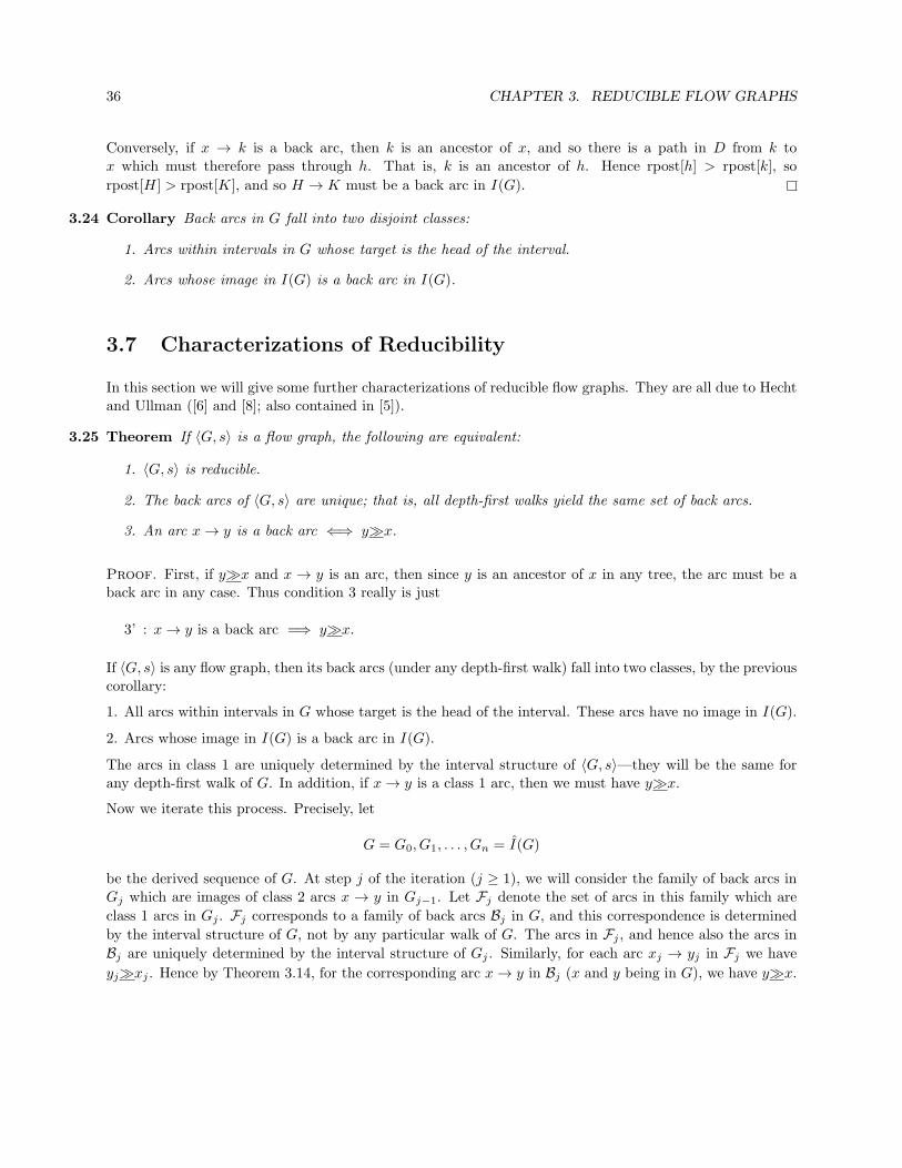
3.24 Corollary Back arcs in G fall into two disjoint classes:
1. Arcs within intervals in G whose target is the head of the interval.
2. Arcs whose image in I(G) is a back arc in I(G).
3.7 Characterizations of Reducibility
In this section we will give some further characterizations of reducible flow graphs. They are all due to Hechtand Ullman ([6] and [8]; also contained in [5]).
3.25 Theorem If 〈G, s〉 is a flow graph, the following are equivalent:
1. 〈G, s〉 is reducible.
2. The back arcs of 〈G, s〉 are unique; that is, all depth-first walks yield the same set of back arcs.
3. An arc x→ y is a back arc ⇐⇒ y≫x.
Proof. First, if y≫x and x → y is an arc, then since y is an ancestor of x in any tree, the arc must be aback arc in any case. Thus condition 3 really is just
3’ : x→ y is a back arc =⇒ y≫x.
If 〈G, s〉 is any flow graph, then its back arcs (under any depth-first walk) fall into two classes, by the previouscorollary:
1. All arcs within intervals in G whose target is the head of the interval. These arcs have no image in I(G).
2. Arcs whose image in I(G) is a back arc in I(G).
The arcs in class 1 are uniquely determined by the interval structure of 〈G, s〉—they will be the same forany depth-first walk of G. In addition, if x→ y is a class 1 arc, then we must have y≫x.
Now we iterate this process. Precisely, let
G = G0, G1, . . . , Gn = I(G)
be the derived sequence of G. At step j of the iteration (j ≥ 1), we will consider the family of back arcs inGj which are images of class 2 arcs x → y in Gj−1. Let Fj denote the set of arcs in this family which are
class 1 arcs in Gj . Fj corresponds to a family of back arcs Bj in G, and this correspondence is determined
by the interval structure of G, not by any particular walk of G. The arcs in Fj , and hence also the arcs in
Bj are uniquely determined by the interval structure of Gj . Similarly, for each arc xj → yj in Fj we have
yj≫xj . Hence by Theorem 3.14, for the corresponding arc x→ y in Bj (x and y being in G), we have y≫x.

3.7. CHARACTERIZATIONS OF REDUCIBILITY 37
If G is reducible, then I(G) is the trivial flow graph, which has no back arcs. Hence every back arc in G willbe in one of the sets Bj . Thus 1 =⇒ 2 and 3.
Conversely, if 〈G, s〉 is not reducible, then it contains a (∗) sub flow graph. If we begin a depth-first spanningtree by following the paths SRPQ, then all the arcs which make up path P will be tree arcs, and the lastarc in Q will be a back arc. On the other hand, if we begin the tree by following the paths STQP , then allthe arcs which make up path Q will be tree arcs and the last arc in P wil be a back arc. Thus, the backarcs will not be unique. Similarly, it is clear that property 3 does not hold for either of the back arcs in Por Q. So properties 2 and 3 each imply property 1.
If 〈G, s〉 is not reducible, then not only is the set of back arcs not unique, the number of back arcs may notbe unique. For instance, Figure 3.7 shows an irreducible flow graph together with two walks which yielddifferent numbers of back arcs.
(1,1)
(4,3)
(3,4)
(2,2)
F
C
B
T
T
T
(1,1)
(2,2)
(3,3)
(4,4)
T
T
T
T
T
T
This irreducible flow graph has either 1 or 2 back arcs, depending on which way it is walked. Asbefore, the pairs of numbers at each node are the pre-order and reverse post-order numberingsof that node.
Figure 3.7: Two Walks of an Irreducible Flow Graph
It is also possible for an irreducible flow graph (i.e. a non-trivial limit flow graph) to have a back arc x→ ywhere y dominates x; it just can’t have that property for all its back arcs. See Figure 3.8 for an example.
We say that a DAG of a flow graph 〈G, s〉 is a maximal acyclic sub flow graph.
3.26 Lemma Any DAG 〈H,E, s〉 of a flow graph 〈G, s〉 includes all the nodes of G.
Proof. If not, there must be an arc x→ y with x ∈ H and y /∈ H. But then adjoining y to H and x→ yto E still keeps 〈H,E, s〉 acyclic.
3.27 Theorem A flow graph 〈G, s〉 is reducible iff it has a unique DAG.
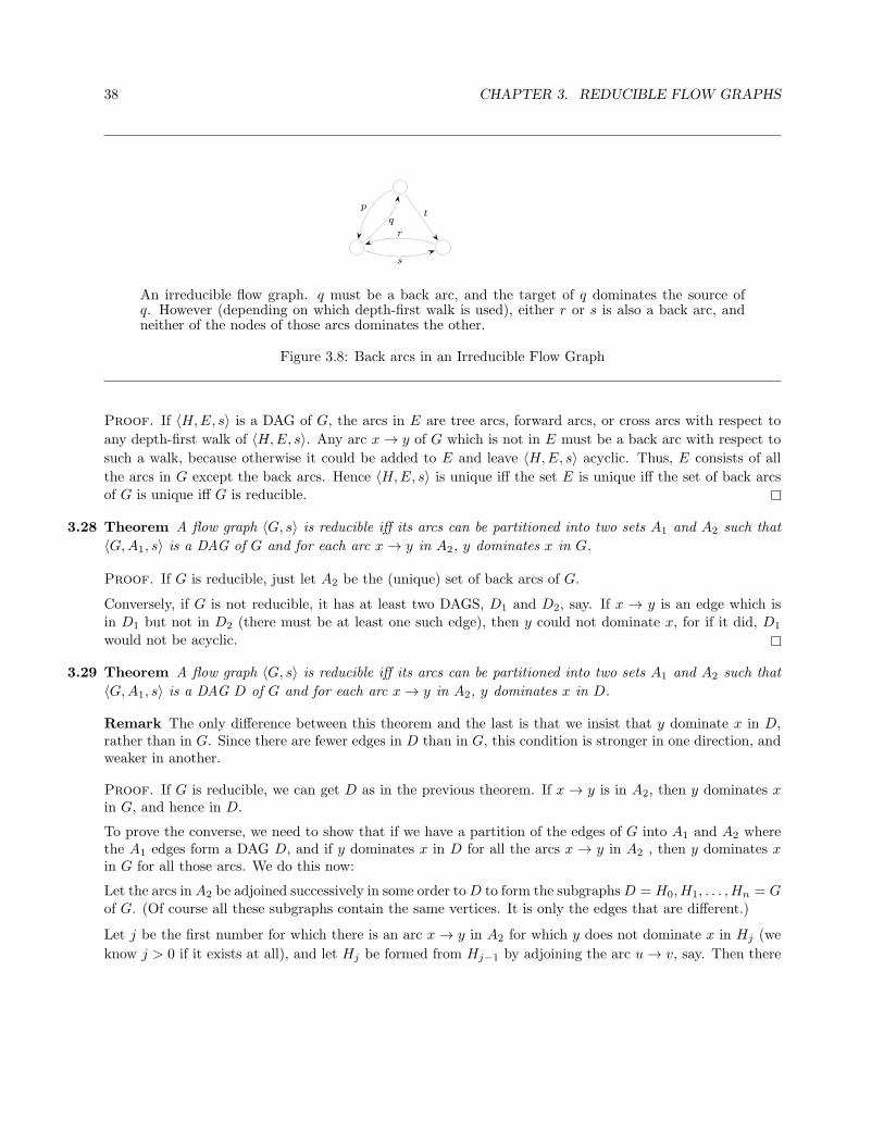
38 CHAPTER 3. REDUCIBLE FLOW GRAPHS
tp
q
r
s
An irreducible flow graph. q must be a back arc, and the target of q dominates the source ofq. However (depending on which depth-first walk is used), either r or s is also a back arc, andneither of the nodes of those arcs dominates the other.
Figure 3.8: Back arcs in an Irreducible Flow Graph
Proof. If 〈H,E, s〉 is a DAG of G, the arcs in E are tree arcs, forward arcs, or cross arcs with respect to
any depth-first walk of 〈H,E, s〉. Any arc x→ y of G which is not in E must be a back arc with respect to
such a walk, because otherwise it could be added to E and leave 〈H,E, s〉 acyclic. Thus, E consists of all
the arcs in G except the back arcs. Hence 〈H,E, s〉 is unique iff the set E is unique iff the set of back arcsof G is unique iff G is reducible.
3.28 Theorem A flow graph 〈G, s〉 is reducible iff its arcs can be partitioned into two sets A1 and A2 such that
〈G,A1, s〉 is a DAG of G and for each arc x→ y in A2, y dominates x in G.
Proof. If G is reducible, just let A2 be the (unique) set of back arcs of G.
Conversely, if G is not reducible, it has at least two DAGS, D1 and D2, say. If x → y is an edge which isin D1 but not in D2 (there must be at least one such edge), then y could not dominate x, for if it did, D1
would not be acyclic.
3.29 Theorem A flow graph 〈G, s〉 is reducible iff its arcs can be partitioned into two sets A1 and A2 such that
〈G,A1, s〉 is a DAG D of G and for each arc x→ y in A2, y dominates x in D.
Remark The only difference between this theorem and the last is that we insist that y dominate x in D,rather than in G. Since there are fewer edges in D than in G, this condition is stronger in one direction, andweaker in another.
Proof. If G is reducible, we can get D as in the previous theorem. If x→ y is in A2, then y dominates xin G, and hence in D.
To prove the converse, we need to show that if we have a partition of the edges of G into A1 and A2 wherethe A1 edges form a DAG D, and if y dominates x in D for all the arcs x → y in A2 , then y dominates xin G for all those arcs. We do this now:
Let the arcs in A2 be adjoined successively in some order toD to form the subgraphsD = H0, H1, . . . , Hn = Gof G. (Of course all these subgraphs contain the same vertices. It is only the edges that are different.)
Let j be the first number for which there is an arc x→ y in A2 for which y does not dominate x in Hj (we
know j > 0 if it exists at all), and let Hj be formed from Hj−1 by adjoining the arc u→ v, say. Then there

3.8. THE LOOP-CONNECTEDNESS NUMBER 39
is a simple path P from s to x in Hj which avoids y, and this path must include the arc u→ v exactly once.
Hence the initial part P1 of this path, from s to u is composed only of arcs in Hj−1. Since P is simple, P1
cannot include v. But this means that v does not dominate u in Hj−1, a contradiction.
3.8 The Loop-Connectedness Number
If G is reducible, the length dsl(G) of the derived sequence of G (the derived sequence length) can be thought
of as the maximum loop nesting depth in G. A famous empirical study performed by Knuth[14] showed that
dsl(G) was almost always bounded by 3. For the analysis of a data-structure algorithm below (see page 81),we will find it useful to estimate a related quantity:
For any flow graph G, we define lc(G) to be the largest number of back arcs (with respect to a fixed depth-
first walk of G) that are contained in any cycle-free path of G. Since there are only finitely many cycle-free
arcs in G, lc(G) is well-defined and finite. lc(G) is called the loop-connectedness number of G. Of course if
G is reducible, lc(G) is a property of G alone, and is independent of the particular depth-first walk.
As usual, I(G) will denote the derived graph of G.
3.30 Lemma lc(I(G)) ≥ lc(G)− 1.
Proof. Let P be a cycle-free path in G with m = lc(G) back arcs. Let the back arcs in P be (in order)
x1 → r1, x2 → r2, . . . , xm → rm
where ri occurs before xi+1 in P . Since P is simple, the {rj} are all distinct. By Corollary 3.21 (page 33),
each ri is therefore the header of a distinct interval.
Let P ′ be the sub-path of P from r1 to rm. The image of P ′ in I(G) must be simple, because otherwise P ′
(which starts at an interval header) would have to enter the same interval twice, and so would not be simple.
Since P is simple, and since for all i the sub-path from ri to ri+1 starts in I(ri) and ends in I(ri+1), it must
enter I(ri+1) at ri+1. Thus for 1 ≤ i < m, xi+1 is not in I(ri+1), and so the image of xi+1 → ri+1 in I(G)
is a back arc. Thus the image of P ′ in I(G) contains at least m− 1 back arcs.
3.31 Theorem If G is a reducible flow graph with loop-connectedness number lc(G) and derived sequence length
dsl(G), then
lc(G) ≤ dsl(G).
Proof. Apply the lemma repeatedly. Since G is reducible, after dsl(G) iterations, we will arrive at a trivial
flow graph for which both dsl and lc are 0. But we subtracted 1 at most dsl(G) times from lc(G) to get to0.
In fact, lc(G) can be much less than dsl(G). For instance, Figure 3.9 shows two flow graphs. The graph on
the left corresponds to three nested repeat loops (in the sense of Pascal; the loop always iterates at least
once, and the test is at the bottom of the loop); the graph on the right corresponds to three nested while
loops (equivalently, Fortran do loops). In both cases, dsl(G) = 3. But for the repeat loop nest, lc(G) = 1,
while for the while loop nest, lc(G) = 3. Thus, while loops keep adding to lc(G), but nests of repeat loopsreally have no effect on it.

40 CHAPTER 3. REDUCIBLE FLOW GRAPHS
The flow graph on the left represents three nested repeat loops (with the test at the bottom ofthe loop); it has dsl(G) = 3 and lc(G) = 1. The flow graph on the right represents three nestedwhile loops (equivalently, Fortran do loops); it also has dsl(G) = 3 but has lc(G) = 3.
Figure 3.9: Nested Loops
3.9 Interval Nesting
Of course, there is no such thing as interval nesting. We know that intervals form a disjoint partition of G.However, each interval in the derived graph I(G) is composed of a number of intervals in G, and so on; soin this sense there is a nesting of lower order intervals in higher order ones. This use of the term “nesting”reflects what we mean when we talk about loop nesting. See, for instance the flow graph on the left ofFigure 3.9.
Let
G = G0, G1, . . . , Gn = I(G)
be the derived sequence of G. Let us refer to an interval in Gj as an interval of order j+1. (It is an element
of Gj+1.) Each such interval can be considered as being composed of a certain number of elements of G,
and in a similar way, the header of such an interval can be associated with an element of G (which is the
header of an ordinary, or order-1, interval of G). Naming intervals by their headers and their order, we canindicate the nesting of lower order intervals in higher order intervals by means of a tree.
For instance, Figure 3.10 shows the derived sequence of a reducible flow graph. Figure 3.11 shows thecorresponding nesting tree for intervals of all orders.
Now let us identify intervals of different orders which share the same header. We will do this by removing
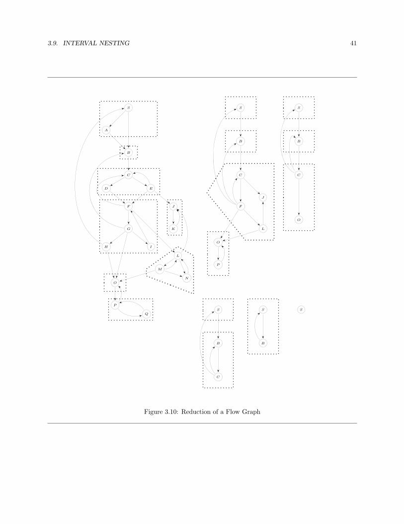
3.9. INTERVAL NESTING 41
S
A
B
C
D E
F
G
H I
J
K
L
M
N
O
P
Q
S
B
C
F
J
L
O
P
S
B
C
O
S
B
C
S
B
S
Figure 3.10: Reduction of a Flow Graph
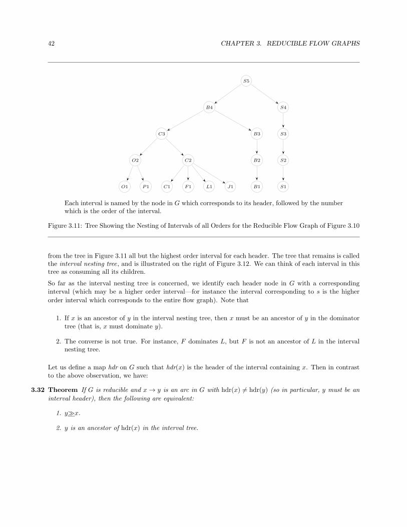
42 CHAPTER 3. REDUCIBLE FLOW GRAPHS
O1 P1
O2
C1 F1 L1 J1
C2
C3
B1
B2
B3
B4
S1
S2
S3
S4
S5
Each interval is named by the node in G which corresponds to its header, followed by the numberwhich is the order of the interval.
Figure 3.11: Tree Showing the Nesting of Intervals of all Orders for the Reducible Flow Graph of Figure 3.10
from the tree in Figure 3.11 all but the highest order interval for each header. The tree that remains is calledthe interval nesting tree, and is illustrated on the right of Figure 3.12. We can think of each interval in thistree as consuming all its children.
So far as the interval nesting tree is concerned, we identify each header node in G with a correspondinginterval (which may be a higher order interval—for instance the interval corresponding to s is the higher
order interval which corresponds to the entire flow graph). Note that
1. If x is an ancestor of y in the interval nesting tree, then x must be an ancestor of y in the dominatortree (that is, x must dominate y).
2. The converse is not true. For instance, F dominates L, but F is not an ancestor of L in the intervalnesting tree.
Let us define a map hdr on G such that hdr(x) is the header of the interval containing x. Then in contrastto the above observation, we have:
3.32 Theorem If G is reducible and x→ y is an arc in G with hdr(x) 6= hdr(y) (so in particular, y must be an
interval header), then the following are equivalent:
1. y≫x.
2. y is an ancestor of hdr(x) in the interval tree.

3.9. INTERVAL NESTING 43
Q
P
O
H I
G
M N
L
F
K
JD E
C
BA
S
P
O F L J
C
B
S
Figure 3.12: The Dominator Tree and the Interval Nesting Tree for the Flow Graph of Figure 3.10
Proof. First of all, if z → w is any arc in G, let zi → wi denote its image in Gi. Of course, zi might equalwi, and since G is reducible, we know that in any case zn = wn.
1 =⇒ 2: We know that x→ y is a back arc. As in the proof of Theorem 3.25 (page 36), the back arcs of G
are partitioned into disjoint sets {Bj}, where each arc z → w in Bj has an image zj → wj in Gj such that
wj is an interval header in Gj and zj is in that interval. (That is, zj → wj is a back arc in an interval of
Gj .) Say x→ y falls in the set Bk. Then y is the header of an interval Iy of order k + 1.
x is a member of the set xk, which is an element of Iy. Hence hdr(x) must also be a member of xk, and
so is a descendant of xk in the interval nesting tree. But we know that xk is a member of Iy, and so is a
descendant of y in the interval nesting tree.
2 =⇒ 1: Since y is an ancestor of hdr(x) in the interval nesting tree, y dominates hdr(x), and hence also
dominates x. (This is just the affirmative part of the observation made earlier.)
The arcs described by this theorem can be characterized as the arcs which are exits from intervals to largercontaining intervals (“interval” in this sense again meaning interval of any order).
Figure 3.13 shows the actual interval nesting in the flow graph corresponding to the interval nesting tree ofFigure 3.12 for the flow graph of Figure 3.10.

44 CHAPTER 3. REDUCIBLE FLOW GRAPHS
S
A
B
C
D E
F
G
H I
J
K
L
M
NO
P
Q
Figure 3.13: Interval Nesting for the Flow Graph of Figure 3.10
Chapter 4
Testing for Reducibility
4.1 Finite Church-Rosser Transformations
If S is a set and =⇒ is a relation on that set (written a =⇒ b), then we say that a sequence
a0 =⇒ a1 =⇒ . . . =⇒ ak
is a chain from a0 to ak of length k. (We think of these chains as chains of implications or of derivations.)
We write a∗
=⇒ b to indicate that there is a chain from a to b.
We say that the relation =⇒ is finite iff for each a ∈ S there is a bound on the length of chains a =⇒b =⇒ . . . beginning with a. That is, =⇒ is finite iff for each a ∈ S, there is an n ∈ N such that if
a =⇒ a1 =⇒ . . . =⇒ ak
with all ai distinct, then k ≤ n. We will call the maximum length of such chains the height of a, and denoteit by h(a). It is clear that if a =⇒ b then h(a) ≥ h(b) + 1. If h(x) = 0, we will refer to x as alimit point ,because there is no other point reachable from x via the relation =⇒ .
The completion =⇒ of the relation =⇒ is the relation defined by right-maximal chains; that is, a =⇒ b iff
there is a chain from a to b and there is no c 6= b with b =⇒ c. Equivalently, a =⇒ b iff b is a limit pointand there is a chain from a to b.
We say that the relation =⇒ is a finite Church-Rosser transformation iff it is finite and =⇒ is a function.
That is, =⇒ is FCR iff it is finite and if a =⇒ b and a =⇒ c implies b = c.
4.1 Theorem (Aho, Sethi, and Ullman[2]) A relation =⇒ on a set S is a finite Church-Rosser transfor-mation iff
1. =⇒ is finite; and
2. for all a ∈ S, if a =⇒ b and a =⇒ c, then there is an x ∈ S such that b∗
=⇒ x and c∗
=⇒ x.
45

46 CHAPTER 4. TESTING FOR REDUCIBILITY
Proof. A finite Church-Rosser transformation certainly satisfies conditions 1 and 2. So we only have toprove that a relation satisfying 1 and 2 is a finite Church-Rosser transformation.
We will prove this by induction on the height of a. That is, given 1 and 2, we will prove the followingstatement:
(P ) If h(a) ≤ k, and if a =⇒ b and a =⇒ c then b = c.
for all k.
(P) is trivially true for k = 1. Suppose it has been proved true for all k < n. Let a be any element of S with
height n, and say a =⇒ b and a =⇒ c. Thus we have chains
a =⇒ b1 =⇒ b2 =⇒ . . . =⇒ b
a =⇒ c1 =⇒ c2 =⇒ . . . =⇒ c
each of length ≤ n, where h(b) = h(c) = 0. By property 2 (since a =⇒ b1 and a =⇒ c1), we then havechains
b1 =⇒ β2 =⇒ β3 =⇒ . . . =⇒ x
c1 =⇒ γ2 =⇒ γ3 =⇒ . . . =⇒ x
We may assume without loss of generality that x is a limit point: otherwise, we could simply continue bothchains in the identical manner until a limit point was attained. But now we have
b1 =⇒ b and b1 =⇒ x
and h(b1) < h(a) = n, so by the inductive assumption, b = x. Similarly, c = x, and so b = c, and we aredone.
4.2 The Transformations T1 and T2
We define two transformations T1 and T2 on flow graphs as follows:
1. T1 is the removal of a self-loop. That is, if x → x is an arc in 〈G, s〉, then T1〈G, s〉 is the flow graph
whose nodes are the nodes of G and whose arcs are all the arcs of 〈G, s〉 except for the arc x→ x.
2. If x 6= y and x is the only predecessor of y in 〈G, s〉, and if y 6= s, then the transformation T2 creates
a new flow graph G′ by “collapsing” y into x. Precisely, the nodes of G′ are all the nodes of G exceptfor y, and the arcs of G′ are
• all the arcs of G not involving y;
• an arc x → b for each arc y → b in G. (In particular, if there is an arc y → x in G, then G′
contains a self-loop x→ x.)

4.2. THE TRANSFORMATIONS T1 AND T2 47
When T2 is applied in this fashion, we say that x consumes y.
In general, we will say that the flow graph G′ is produced by collapsing the flow graph G if G′ is producedfrom G by a series of transformations of the form T1 and/or T2.
Of course the transformations T1 and T2 are really not uniquely defined: if there are several self-loops in〈G, s〉, T1 could be applied to any of them; and similarly for T2. They actually define a relation on the set
of flow graphs. We can imagine applying these transformations repeatedly on a flow graph 〈G, s〉 until wecan go no further. We will show that the flow graph that we get by doing this is always the limit flow graphof 〈G, s〉, no matter in what order the transformations were applied. In particular, a flow graph is reducibleiff it can be transformed to the trivial flow graph by successive applications of T1 and T2, in any order.
The transformations T1 and T2 are due to Hecht and Ullman[6].
4.2 Theorem The relation =⇒ defined on the set of flow graphs by the transformations T1 and T2 is a finiteChurch-Rosser transformation.
Proof. First, the relation is finite, since T1 and T2 each reduce the number of arcs by at least 1. So thelength of a chain starting at 〈G, s〉 can be at most the number of arcs in 〈G, s〉.
Now suppose we have GTi=⇒L and G
Tj=⇒M . We want to show that the following diagram can be produced:
GTi=⇒ Lww�Tj
ww�∗M
∗=⇒ H
Case I: i = j = 1. If T1 was applied to node x to yield L and to node y to yield M , then
• if x = y, then L =M , and we are done.
• otherwise, T1 can be applied to y in L and to x in M , yielding the same graph H in each case.
Case II: i = j = 2. Say x consumes y to yield L and z consumes w to yield M :
x zyy
y w
We know that in any case x 6= y and z 6= w.
• If y = w, then x must equal z, since y has a unique predecessor in 〈G, s〉. Hence L =M already.In all the remaining cases, y 6= w.
• If all four nodes are distinct, then x can consume y in M and z can consume w in L to yield thesame graph H.
• If x = z, then x can consume w in L and x can consume y in M to yield the same graph H.
• If x = w but z 6= y, then z can consume x in L and z can consume y in M to yield the samegraph H.
All other possible cases are symmetric versions of these cases.
48 CHAPTER 4. TESTING FOR REDUCIBILITY
Case III: i 6= j. Say x consumes y to yield L (via T2) and T1 is applied to z to yield M . y cannot equal
z. Hence x can still consume y in M , and T1 can be applied to z (which might be x) in L, in eithercase yielding the same graph H.
Therefore, we see that it does not matter in which order (or to which nodes or arcs) we apply the transfor-
mations T1 and T2—if we start with a flow graph 〈G, s〉 and keep on going until we can go no farther, wewill arrive at a unique graph depending only on G.
4.3 Lemma Any pre-interval can be collapsed to its header by a series of T2 operations, followed by at mostone T1 operation. Any arcs from the original pre-interval to other nodes become arcs from the header tothose same nodes.
Proof. Let 〈H,h〉 be any pre-interval in G. There must be at least one node x 6= h in H such that x has
only one predecessor (y, say), for if each node in H other than h had two predecessors, then one of themwould not be h, and by following arcs backward through H, always choosing the predecessor which was noth, we would eventually create a loop in H not containing h, a contradiction.
So if x is such a node, then T2 can be applied to collapse x into y, turning H into H ′, say. Any arcs from xleading outside H now become arcs from y ∈ H ′ to the same target. After this application of T2, 〈H ′, h〉 is
still a pre-interval, for it still has the unique entry node h, and if C is a cycle in H ′ not including h, then Cmust include y (otherwise C would have been a cycle in H). Say C looks like this:
c0 → c1 → . . .→ ck−1 → y → ck+1 → . . .→ cn = c0.
There could not be an arc y → ck+1 in H, for then again C would be a cycle in H. Hence the arc y → ck+1
must come from an arc x→ ck+1 in H. But then replacing y in C by y → x yields a cycle in H not includingh, a contradiction.
If we apply this process repeatedly, we will wind up with H collapsed to its header, with possibly a self-loopat the header. This self-loop can be eliminated by applying T1. Thus H is replaced by its header, and everyarc from an element of H to a target outside H is replaced by an arc from its header to the same target.
While the above proof was a pure existence proof (in fact, a proof by contradiction), we will see below
(Theorem 4.8 on page 50) that there actually is an algorithm for generating the sequence of T2 reductionsof any pre-interval
4.4 Lemma G∗
=⇒ I(G).
Proof. Applying Lemma 4.3 in turn to each interval in G yields I(G).
4.5 Theorem G =⇒ I(G).
Remark That is, the result of applying T1 and T2 repeatedly to G until neither can be applied any moreis the limit graph of G; and in particular, G is reducible iff it can be reduced to the trivial flow graph bysuccessive applications of T1 and T2.
Proof. Applying Lemma 4.4 repeatedly, we get G∗
=⇒ I(G). So all we have to prove is that I(G) is a limitpoint in the set of flow graphs under the transformations T1 and T2.

4.3. INDUCED WALKS FROM T1 AND T2 49
First, derived flow graphs by construction do not contain self-loops. Hence T1 cannot be applied to I(G).
Next, since I(G) is a limit flow graph, all its pre-intervals are trivial (i.e. consist of just one node). If
there were an element x of I(G) which had a unique predecessor y, then 〈{y, x}, y〉 would be a non-trivial
pre-interval in I(G), a contradiction. Hence T2 cannot be applied to I(G).
4.3 Induced Walks from T1 and T2
Now let us say that G is transformed into G′ by an application of T1 or T2. If D is a depth-first spanningtree of G (corresponding to a depth-first walk of G), then D has an image D′ in G′.
Case I. T1 was applied to get G′. Since all self-loops are back arcs, D′ is the same as D, and the pre- andpost-orderings of the nodes of G′ are the same as those of G.
Case II. T2 was applied to get G′. Say T2 was applied to the arc a→ b in G. The arc a→ b was the onlyarc to b. Hence it must be a tree arc. So D′ is D without this arc (and with a and b identified). D′
is still a tree because every element except s in G′ has exactly one arc in D′ entering it. There is aninduced walk on D′ which can be described as follows:
• Each node which was visited before b is visited in the same order. This includes all the nodesvisited up to a, and those children of a which were visited before b.
• Then the descendants of b are visited in the same order.
• Then the subtrees rooted at the remaining children of a (after b) are visited in the same order.
• Finally, the rest of the tree is visited in the same order.
That is, the tree is walked until b would have been reached; it is skipped over, and the remainingnodes are visited in the same order. Thus, if nodes in G are denoted by {x, y, . . .} and nodes in G′ are
denoted by {x′, y′, . . .}, then
pre[x] < pre[b] =⇒ pre[x′] = pre[x]
pre[x] > pre[b] =⇒ pre[x′] = pre[x]− 1
If G has n nodes, then G′ has n− 1 nodes. If the post-order number of a node is denoted by post[x],then we have
rpost[x] + post[x] = n; rpost[x′] + post[x′] = n− 1.
Now
rpost[x] < rpost[b] ⇐⇒ b is finished being processed before x
⇐⇒ post[b] is assigned before post[x]
⇐⇒ post[x′] = post[x]− 1
⇐⇒ rpost[x′] = rpost[x]

50 CHAPTER 4. TESTING FOR REDUCIBILITY
and similarly,
rpost[x] > rpost[b] ⇐⇒ x is finished being processed before b
⇐⇒ post[x] is assigned before post[b]
⇐⇒ post[x′] = post[x]
⇐⇒ rpost[x′] = rpost[x]− 1
4.6 Theorem If x and y are nodes in G whose images in G′ are x′ and y′, then
1. pre[x] < pre[y] =⇒ pre[x′] ≤ pre[y′].
2. rpost[x] < rpost[y] =⇒ rpost[x′] ≤ rpost[y′].
If x′ 6= y′ then
1. pre[x] < pre[y] ⇐⇒ pre[x′] < pre[y′].
2. rpost[x] < rpost[y] ⇐⇒ rpost[x′] < rpost[y′].
Proof. Follows immediately from the calculations above.
4.7 Theorem If x→ y is an arc in G which corresponds to an arc x′ → y′ in G′, then either they are both backarcs or neither is.
Proof. 1. If T1 was applied to yield G′, the pre- and post-orderings of all the nodes are unchanged, andtree arcs are preserved, so the character of all the arcs (except of course the deleted one) is unchanged. So
let us assume that T2 was applied to yield G′.
2. If x′ and y′ are identified in G′, then a back arc x → y must become a self-loop x′ → x′ in G′, which isautomatically a back arc. Similarly, if x′ and y′ are identified in G′, then a self-loop x′ → x′ in G′ couldonly have come from a back arc in G.
3. If x′ and y′ are distinct in G′, then
x→ y is a back arc in G ⇐⇒ pre[x] > pre[y] and rpost[x] > rpost[y]
⇐⇒ pre[x′] > pre[y′] and rpost[x′] > rpost[y′]
⇐⇒ x′ → y′ is a back arc in G′
We also note that x′ is a descendant of y′ in G′ (with respect to D′) iff x is a descendant of y in G (with
respect to D).
Now as promised, we can show that a pre-interval can be collapsed by T2 transformations in an easilycalculated order: the order in fact is just reverse post-order:
4.8 Theorem If the flow graph 〈G, s〉 is numbered by a depth-first walk, then any pre-interval 〈H,h〉 in G, can
be collapsed to its header by applying T2 transformations successively to each node in H − {h} in reverse
post-order, followed possibly by one T1 operation on h. Any arcs from the original pre-interval 〈H,h〉 toother nodes become arcs from the header h to those same nodes.

4.4. KERNELS OF INTERVALS 51
Proof. First, since h dominates every element of H, rpost[h] < rpost[x] for all x ∈ H.
Let x be the element of H − {h} such that rpost[x] is smallest. If y → x is an arc, then rpost[y] < rpost[x],since otherwise y → x would be a back arc, and the only back arcs in H have h as their target. But thensince rpost[x] is minimal, we must have y = h. Thus, the only arc whose target is x is h→ x. Hence T2 canbe applied to collapse x into h.
By Theorem 4.6, the reverse post-ordering of the nodes of H is not changed by this application of T2. Thesame argument can then be iterated to visit all the nodes of H − {h} in reverse post-order, collapsing eachin turn into h.
As in Lemma 4.3, at most one application of T1 to h will then complete the collapse of 〈H,h〉 to the singlenode h.
4.4 Kernels of Intervals
In general, an interval consists of zero or more loops (each including the interval header), and additional
non-cyclic structures hanging off the loops (or off the header if there are no loops). The loops are the essentialpart of the flow graph: without loops, computations of data flow are very easy. So let us refer to the looppart of an interval as the “kernel” of an interval. First we show that the kernel exists unambiguously. Clearlywe want the loop part of an interval to be strongly connected and to include the interval header. We usethis idea to characterize the kernel.
4.9 Lemma The family H of strongly connected subsets of a pre-interval 〈H,h〉 which include h has a maximalelement which includes all the members of H.
Proof. Since {h} ∈ H, H 6= ∅. Clearly the union of any two members of H is a member of H. Since H isfinite, the union of all the members of H is maximal and includes every member of H.
Now we define the kernel of a pre-interval 〈H,h〉 to be the maximal strongly connected subset of H which
includes h. We will use the notation k(H) or k〈H,h〉 to refer to the kernel of the pre-interval 〈H,h〉.
4.10 Lemma The kernel of a pre-interval 〈H,h〉 consists of all elements x of H for which there is a path in Hfrom x to h.
Proof. Call this set C. Since k(H) is strongly connected, k(H) ⊂ C. Conversely, if x ∈ C then since 〈H,h〉is a pre-interval, there is a path P in H from h to x. Every element y in this path is in C, since the pathcan be followed from y to x, and then there is a path from x to h. Hence every element of C can be reachedfrom h by a path in C, and so C is strongly connected. By maximality, then, C ⊂ k(H).
In particular, by Theorem 3.20, k(H) includes all the back arcs in H.
4.11 Lemma The kernel of a pre-interval with header h is a pre-interval with header h.
Proof. We know that h ∈ k(H). If a ∈ k(H), a 6= h, and a is the target of an arc b → a, then b must be
in H. Since there is then a path in H from b to h, b must be in k(H). Thus, the only entry to k(H) is at h.
There can be no cycles in k(H) which do not include h since k(H) is a subset of H.

52 CHAPTER 4. TESTING FOR REDUCIBILITY
Thus the kernel of each interval can be collapsed by Lemma 4.3. After its kernel has been collapsed, eachinterval has no remaining back arcs (by Theorem 4.7) and so is a DAG. There still may be back arcs inthe graph, however: these correspond to back arcs between intervals in the original graph. Let us denotethe graph generated by collapsing the kernel of each interval of G by J(G). Just as we iterated the map
G→ I(G) to get a limit graph I(G) when defining reducibility, we can iterate the map G→ J(G) to get a
limit graph J(G). Figure 4.1 shows the construction of J(G) for the flow graph of Figure 3.3.
Figure 4.1: Successive Kernel Reductions for the Graph of Figure 3.3
More generally, let T3 be a transformation on a flow graph which consists of collapsing the kernel of 1 ormore intervals of that graph. In particular, J(G) is produced by the action of one version of T3 on G, namelythe version of T3 which collapses the kernels of all the intervals of G.
It seems likely to me that the family of T3 transformations is a finite Church-Rosser system, and so any
T3-limit graph of G is equal to J(G). For our purposes, however, we don’t need this strong result. A simplecharacterization of reducibility in terms of T3-limit graphs is all we need:
4.12 Theorem G is reducible iff J(G) is a DAG.
Proof. First of all, by Theorem 4.5, G is reducible iff J(G) is reducible. So we have to show that J(G) is
reducible iff it is a DAG. Since any DAG is reducible (the whole graph is an interval), we only have to show
that if J(G) is reducible, it must be a DAG.
If J(G) is not a DAG, it contains a back arc (with respect to some depth-first walk). Let x→ y be the back

4.5. REACHUNDER SETS AND TARJAN’S ALGORITHM 53
arc such that pre[y] is maximal1. Let H be the union of the nodes on all simple paths from y to x. Since
J(G) is assumed to be reducible, y must dominate x, and so y must dominate every node in H. Further,there cannot be any cycles in H not including y, for if so, there would be a back arc a→ b with a and b inH and b 6= y. But since y dominates b, pre[y] < pre[b], which contradicts the maximality of pre[y] among all
targets of back arcs. Hence H is a pre-interval with header y, and x ∈ k(H). But this means that J(G) isnot invariant under J , a contradiction.
4.13 Corollary G is reducible iff any sequence of applications of T3 can be extended with 0 or more applicationsof T3 to yield a DAG.
Proof. Since T3 consists of applications of T1 and T2, G is reducible iff it remains reducible after anysequence of applications of T3. Now apply the Theorem.
4.14 Corollary If 〈G, s〉 is a flow graph, the following are equivalent:
1. G is reducible.
2. Some T3-limit graph formed starting with G is a DAG.
3. Every T3-limit graph formed starting with G is a DAG.
In particular, we can test a flow graph for reducibility by collapsing the kernel of just one interval, thencollapsing the kernel of just one interval in the resulting graph, and so on. The graph will be reducible iffwe eventually come to a DAG.
4.5 Reachunder Sets and Tarjan’s Algorithm
Tarjan gave an algorithm to test for flow graph reducibility based on these ideas. His algorithm uses what wewill call a “reachunder” set, which is more or less equivalent to what we have called the interval kernel—itactually could include the kernels of several intervals.
Definition Let 〈G, s〉 be a flow graph, and let there be a depth-first spanning tree chosen for 〈G, s〉. If x is
the target of a back arc in G, the reachunder set of x, ρ(x), is the set of those elements y such that there is
a simple path from y to x, the last arc of which is a back arc.2
In particular, x /∈ ρ(x). Of course, if there is no back arc whose target is x, then ρ(x) = ∅.
Reachunder sets can be used to characterize reducibility:
4.15 Theorem If 〈G, s〉 is a flow graph with a spanning tree D rooted at s, the following are equivalent:
1. G is reducible.
2. For all x ∈ G, x dominates every element in ρ(x).
1That is, maximal with respect to all back arcs. This device is due to Tarjan.2The first use of the term “reachunder” appears to be in the paper by Schwartz and Sharir[16]. Tarjan doesn’t give a name
to the reachunder sets he uses; they occur in his paper (Tarjan[20]) as P (x). The idea of the set goes back at least to Hecht[5]in his proof of our Theorem 3.18. It actually isn’t necessary for that proof, as we have seen.
54 CHAPTER 4. TESTING FOR REDUCIBILITY
3. For all x ∈ G, x is an ancestor (with respect to D) of every element in ρ(x).
Proof. 1 =⇒ 2: Say y ∈ ρ(x). If x does not dominate y, then there is a path in G from s to y avoiding x.
If we adjoin to the end of this path the path in ρ(x) from y to x, we get a path from s to x which does not
contain x in its interior. Therefore, since the last arc in that path is a back arc (z → x, say), we see that xdoes not dominate z and hence G is not reducible.
2 =⇒ 3: If x dominates an element y, then x must be an ancestor of y with respect to each spanning treeof G which is rooted at s.
3 =⇒ 1: If G is not reducible, then with respect to any given depth-first spanning tree D of G, there is aback arc z → x for which x does not dominate z. We know that x 6= s, since s dominates everything. Hencethere is a path in G from s to z which avoids x, and hence s ∈ ρ(x). But certainly x is not an ancestor ofs.
4.16 Lemma If x is the node in G with the greatest pre-order number which is a target of a back arc3, then nodescendant of x is the target of a back arc.
Proof. If b is any descendant of x, we must have pre[x] < pre[b]. Since x is the node with highest pre-ordernumber which is the target of a back arc, b cannot be the target of a back arc.
4.17 Lemma If G is reducible and if x is the node in G with the greatest pre-order number which is the target ofa back arc, then ρ(x) ∪ {x} = k(I(x)).
Proof. Say y → x is a back arc. ρ(x) ∪ {x} must have x as its only entry point because x dominates the
source of every back arc (since G is reducible). Further, there can be no cycles in ρ(x) because otherwise
there would be a back arc in ρ(x), which is impossible by the last lemma. Hence ρ(x)∪ {x} is a pre-interval
with header x, and is therefore contained in I(x). Since by construction it consists of all elements z of I(x)
for which there is a path in I(x) from z to x, Lemma 4.10 shows that ρ(x) ∪ {x} = k(I(x)).
We can now give Tarjan’s algorithm for testing reducibility (Figure 4.2). The algorithm first makes a list of
targets of back arcs in reverse pre-order, v1, . . . , vk (so that pre[v1] is maximal, and the sequence {pre[vi]}
is decreasing). Then it computes ρ(v1). If ρ(v1) contains a non-descendant of v1, the algorithm returns
FALSE. Otherwise, ρ(v1) can be collapsed into v1. Then ρ(v2) is computed (in the collapsed graph), and soon.
When building up ρ, each node added to ρ is checked to make sure that x is an ancestor of it. Hence byLemma 4.16, there can be no back arcs to it. Therefore, when we are building up the set P which willeventually be ρ(v1), we only have to look at tree arcs, forward arcs, and cross arcs entering P . After ρ(v1)has been finished and collapsed into v1, v2 will be the node with the greatest pre-order number which is thetarget of a back arc (in the collapsed graph), and so the same process can be used when building up ρ(v2).
Each reachunder set is identified with its header, which is always the target of one of the original back arcsin G. As the algorithm proceeds, reachunder sets can be formed from nodes which themselves representreachunder sets. In order to manage these set unions, the algorithm uses two functions:
FIND(x) returns the set (i.e. the node in the reduced graph) containing x.
3as in the proof of Theorem 4.12

4.5. REACHUNDER SETS AND TARJAN’S ALGORITHM 55
function REDUCE(〈G, s〉: flow graph): boolean;begin
Construct a depth-first spanning tree D of G, numbering vertices from 1 to n in pre-order and reversepost-order and calculating ND[v] for each vertex v;
for each vertex v (in any order) doMake lists of all back arcs, forward arcs, and cross arcs entering vertex v;Construct a set named v containing v as its only element;HIGHPT[v]← 0;
end for;
for each vertex x in reverse pre-order doP ← ∅;for each back arc y → x do
add FIND(y) to P ;end for;
Q← P ;-- Now construct ρ(x) by exploring backward from vertices in Qwhile Q 6= ∅ do
Select a vertex t ∈ Q and delete it from Q;
for each forward arc, tree arc, or cross arc y → t do
-- All back arcs entering t have already been collapsedy′ ← FIND(y);if pre[x] > pre[y′] or pre[x] + ND(x) ≤ pre[y′] then
return(FALSE); -- G is not reducible.end if ;if y′ ∈ P and y′ 6= x then
Add y′ to P and to Q;end if ;if HIGHPT(y′) = 0 then
HIGHPT(y′)← pre[x];end if ;
end for;
end while;-- Now P = ρ(x) in the current graphfor s ∈ P do
UNION(s, x, x);end for;
end for;return(TRUE);
end
Figure 4.2: Tarjan’s Test for Reducibility

56 CHAPTER 4. TESTING FOR REDUCIBILITY
UNION(A,B,C) creates a set C equal to the union of the sets A and B (destroying A and B in the process).
In addition, an attribute HIGHPT[x] is defined for each node and computed to be the pre-order number of
the first vertex (which must be a target of a back arc) into which x is collapsed (and 0 if x is not collapsed).
For example, for all y ∈ ρ(v1), HIGHPT[y] = pre[v1].
Tarjan’s algorithm gives us a convenient way to specify how a reducible flow graph can be collapsed bysuccessive applications of the T1 and T2 transformations:
Let us define an ordering on the nodes of G, which we will call reduction ordering , as follows: x will precedey iff
1. HIGHPT[x] > HIGHPT[y]; or
2. HIGHPT[x] = HIGHPT[y] and rpost[x] < rpost[y].
4.18 Theorem The flow graph 〈G, s〉 can be reduced by a sequence of T1 and T2 transformations as follows: visitthe nodes in reduction order.
1. Each node can be collapsed by an application of T2 into some other node.
2. All nodes with the same value of HIGHPT are collapsed into the same node.
3. When all the nodes with the same value of HIGHPT have been collapsed (say into node h), then apossible application of T1 to h can be made.
Proof. Consider first all the nodes for which HIGHPT is greatest; this is the initial part of the sequenceof nodes in reduction order. These nodes constitute the first reachunder set formed by Tarjan’s algorithm.By Theorem 4.8, these nodes can be collapsed in reverse post-order (which is the same as reduction order
on this set) by applications of T2. After they have all been collapsed into their header, an application of T1to that header may be needed to delete any self-loop at the header.
We know that the reverse post-ordering of the nodes is not affected by the transformations T1 and T2 (that
is, the actual numbering may change, but the ordering induced by the numbering does not). Hence thisprocess can be iterated on each successive reachunder set until G is completely reduced.
Tarjan has showed that this algorithm can be performed in time
O(Eα(E, V ))
where V and E are the number of vertices and edges in 〈G, s〉 and where α is related to an inverse ofAckermann’s function and grows so slowly that for all practical purposes it is bounded by 3.
An example of the working of this algorithm is shown in Figure 4.3.
Figure 4.4 shows Tarjan‘s algorithm applied to the same reducible flow graph as in Figure 3.10. The limitDAG is shown in the upper right-hand corner, and the nesting tree of reachunder sets (analogous to the
interval nesting tree) is shown at the lower right-hand corner. The root of the nesting tree is the limit DAG.
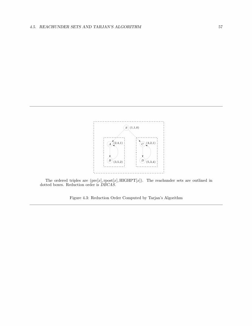
4.5. REACHUNDER SETS AND TARJAN’S ALGORITHM 57
B (3,5,2)
A (2,4,1)
D (5,3,4)
C (4,2,1)
S (1,1,0)
The ordered triples are (pre[x], rpost[x],HIGHPT[x]). The reachunder sets are outlined indotted boxes. Reduction order is DBCAS.
Figure 4.3: Reduction Order Computed by Tarjan’s Algorithm

58 CHAPTER 4. TESTING FOR REDUCIBILITY
S
A
B
C
D E
F
G
H I
J
K
L
M
N
O
P
Q
1
2
3
4
5 18
6
7
812
16
17
13
14
159
1011
F
B
CC
B
B
F
B
B
B
FB
C
B
B
B
S
J
L
O
root
S O L J
B P
C
F
The nodes are numbered in pre-order. Tree arcs are solid lines. Forward arcs (F), cross arcs (C),and back arcs (B) are dashed lines and are labelled. The successive reachunder sets are indicatedby dotted boxes. The reachunder sets are found in the order JLPOFCBS.
The limit graph J(G) is shown at the upper right.
The nesting tree of reachunder sets is shown at the lower right.
Figure 4.4: Tarjan’s Algorithm Applied to the Reducible Flow Graph of Figure 3.10

Chapter 5
Applications to Data-Flow Analysis
5.1 Four Data-Flow Problems
In this chapter, 〈G, s〉 will be understood to be the flow graph of basic blocks in the intermediate represen-tation of a computer program. In addition, although we have not assumed anything about exit nodes inflow graphs (and although programs in general do not have to have unique exit nodes), we will assume that
〈G, s〉 has a unique exit node, which is reachable from every other node. This is no great restriction, for ifa program has more than one exit node, we can simply create a new one and add an arc from each of theformer exit nodes to the new one. And certainly we are not interested in analyzing programs which containnodes which cannot lead to an exit. Let us denote the exit node of the program by e (for “end” or “exit”).
We will denote such a flow graph by 〈G, s, e〉.
Note that a flow graph 〈G, s, e〉 is now defined perfectly symmetrically; and in fact, for each flow graph, there
is a reverse graph 〈G, e, s〉 formed from the same nodes as G by simply reversing the direction of each arc. sand e then change roles. The reverse graph of a reducible flow graph is not necessarily reducible, however;see, for instance, Figure 5.1.
a e
s
a s
e
Figure 5.1: The reverse graph of a reducible flow graph may not be reducible.
For the purposes of global optimization, we wish to gather information about the use of variables in theprogram. The following are typical kinds of information:
Available Expressions An expression such as x+ y is available at a point P in the program iff
• the expression has been computed on each path from s to P ; and
59
60 CHAPTER 5. APPLICATIONS TO DATA-FLOW ANALYSIS
• if the expression were recomputed at P , its value would not be different from the last computedvalue.
For instance, not only must x+ y have been computed previously, but also the values of x and y mustnot have changed since the last computation of x+ y on any path to P . Any change to the values ofx or y is said to “kill” the value of the expression x+ y.
If an expression is available at a point, then in principle, it does not need to be re-evaluated at thatpoint if it occurs there—its value may have been saved in a register. Thus, the more expressions weknow are available at a point, the more useful information we have.
Reaching Definitions A definition of a variable is a statement which can modify the value of the variable;e.g. an assignment to the variable or a read statement. A definition of a variable v reaches the pointP in the program iff there is a path from the definition to P on which v can be shown to be unchanged(i.e. on which there is no other definition of v; another definition of v would be said to “kill” the first
definition). Given a point P in the program, and a variable v, we want to compute the set of definitionsof v which reach P .
If only one definition of a variable reaches a point, then a use of that variable can be replaced by itsdefinition—in particular, the definition may assign a constant value to the variable, and the use of thevariable may thus be replaced by that constant. On the other hand, if more than one definition ofa variable reaches a point, then we can’t perform this kind of replacement. Thus (in contrast to the
situation in the problem of Available Expressions) the fewer definitions of a variable which reach apoint, the more useful information we have.
Another way that reaching definitions information can be used is this: Say E is an expression in thebody of a loop. If all the reaching definitions of E are outside the loop, then E is a loop invariantand can be evaluated once before the loop is entered, rather than each time through the loop. Again,finding fewer reaching definitions constitutes finding more useful information.
Live Variables A variable is live at a point P of the program iff its value at P could be used along somepath leaving P .
Liveness information is used in register allocation. A code generator may generate code assumingan infinite number of “virtual” registers. Each virtual register than has to be assigned to an actualmachine register, and of course this has to be done in such a way that the assignments do not conflict.A modern compiler has a register allocation phase that performs this assignment.
Virtual registers can be classified as local (used entirely within one basic block or global (used in more
than one basic block).
If the machine we are compiling for only has a few registers, it is common to perform only local registerallocation—this means that we allocate registers within each basic block, but do not keep any values inregisters between basic blocks. Thus, any global register used in a basic block will have to be writtento memory at the end of the block, in order to safely preserve its value for use in some subsequentbasic block. However, any virtual register that is not live at the end of a basic block does not have tobe stored in memory—it can be allowed to “die” at the end of the block. So knowing that a virtualregister is not live is useful information. (Note that while the problem is conventionally referred to as
“live variables”, the variables in question are actually the virtual registers.)
If the machine has a sufficiently large number of registers, we may also perform global register allocation.That is, we attempt to assign global virtual registers to machine registers consistently over largersegments of the program. The key point is that a virtual register has to correspond to a machine
5.2. DATA-FLOW EQUATIONS 61
register only at those points in the program at which the virtual register is live. Global registerallocation thus is driven by liveness information. So in this case also, knowing that a virtual registeris not live is useful information, because it frees up a machine register for allocation to another virtualregister: if we have fewer live variables, we have more useful information.
Very Busy Expressions An expression is very busy at a point P of the program iff it is always subsequentlyused before it is killed.
If an expression is very busy at P then it can be computed at P and subsequent computations alongall paths before its first use along each path can be deleted. This process is called “code hoisting”,and saves space, though in general not time. (For this reason, this concept is now only of historical
interest.) The more very busy expressions we have, the more code hoisting we can do, and hence themore useful information we have.
In each of these problems, we may not be able to compute all this useful information perfectly accurately.However, if we compute approximations to the useful information which yield no more than the true usefulinformation (i.e. which are lower approximations to the true useful information), then we will at any rate notperform any unjustified program transformations. Thus, lower approximations to the true useful informationin each case are safe or conservative approximations.
5.2 Data-Flow Equations
The points P of the program at which we are concerned with this information are the beginnings and theends of basic blocks. It turns out that there are some simple relationships or constraints which we can writedown. Each constraint relates four quantities:
in The information valid on entrance to a basic block.
out The information valid on exit from a basic block.
gen The information generated within the basic block.
kill The information killed or made invalid within the basic block.
In each case, the items gen and kill are quantities which we can compute in a straightforward manner foreach basic block (they are functions on the set of basic blocks), and the quantities in and out (which are
also functions on the set of basic blocks) are the final quantities we hope to arrive at.
For example, for the Available Expressions problem, for a given expression and a given basic block, in forthat basic block is a boolean quantity which is TRUE iff that expression is available on entrance to thatbasic block.
In general, for each instance of the four examples of data-flow information given above (that is, for each
expression, or each definition, etc.), these four quantities are boolean functions on basic blocks which are
TRUE as follows (N.B. the precise definitions of gen and kill in each case are determined by the data-flow equations subsequently presented; in particular, the definitions for the Live Variables and Very BusyExpressions problems are tailored to reflect their use in “bottom-up” equations, as we will see below):
Available Expressions For a given expression,
62 CHAPTER 5. APPLICATIONS TO DATA-FLOW ANALYSIS
in The expression is available on entrance to the basic block.
out The expression is available on exit from the basic block.
gen There is an explicit computation of the expression in the basic block which is not followed in thesame basic block by a subsequent change to the value of any variable in the expression (which
would change the value of the expression if it were recomputed).
kill The value of some variable in the expression changes within the basic block (so that if the expres-
sion were recomputed, its value might change), and the expression is not subsequently computedin the basic block.
Reaching Definitions For a given definition,
in The definition reaches the entrance to the basic block.
out The definition reaches the exit from the basic block.
gen The definition is produced within the basic block and not subsequently killed in the same basicblock (by another definition of the same variable).
kill The definition is killed within the basic block (by another definition of the same variable within
that block).
Live Variables For a given variable,
in The variable is live on entrance to the basic block.
out The variable is live on exit from the basic block.
gen The variable is used within the basic block prior to any definition of that variable within theblock. Also called use.
kill The variable is defined within the basic block prior to any use of the variable within the basicblock. Also called def.
Very Busy Expressions For a given expression,
in The expression is very busy on entrance to the basic block.
out The expression is very busy on exit from the basic block.
gen The expression is used within the basic block prior to any definition of any variable in thatexpression within the basic block. Also called use.
kill The value of some variable in the expression changes within the basic block (so that if the ex-
pression were recomputed, its value would be different) prior to any use of the expression in theblock.
Note that in every case, gen ∧ kill = FALSE. This is a convention: we don’t allow information to be bothgenerated and killed within one basic block.
We now can write down some equations involving these quantities. For each basic block b, let pred(b) denote
the family of basic blocks which are predecessors of b (i.e. those basic blocks x for which x→ b is an arc in
the flow graph); and let succ(b) denote the family of basic blocks which are successors of b. We have threekinds of equations:
Boundary value equations These define values at the entry or exit blocks of the program.

5.2. DATA-FLOW EQUATIONS 63
Propagation equations These tell how values are propagated from one basic block to another. These arealso called confluence equations.
Transfer equations These tell how values are changed by a basic block.
There are two general types of data-flow problems: those in which information is propagated in the directionof program execution (forward equations), and those in which equation is propagated in the reverse direction
(backward equations). In general, we let in, out, etc. be represented as boolean vectors (usually referred
to as bit-vectors), with one dimension allocated to each expression, definition, or variable in the problem.
Since boolean vectors are equivalent to subsets, we can denote the vector which is all FALSE by ∅, 0, or ⊥.Although we will not need it till later, we will denote the vector which is all TRUE by 1 or ⊤. Similarly,the boolean operator ∨ will be denoted by ∪, and ∧ will be denoted by ∩. We can therefore interpret thevariables in, out, kill, and gen as the sets of expressions, definitions, or variables which are characterized bythe conditions stated above.
Forward Equations
Available Expressions and Reaching Definitions are both examples of data-flow problems which lead toforward equations:
Available Expressions: The equations are
in(s) = ∅
in(b) =⋂
x∈pred(b)
out(x) for b 6= s
out(b) = (in(b)− kill(b)) ∪ gen(b)
Reaching Definitions: The equations are
in(s) = ∅
in(b) =⋃
x∈pred(b)
out(x) for b 6= s
out(b) = (in(b)− kill(b)) ∪ gen(b)
Thus, forward equations are characterized by passing information from the predecessors of a node to thenode itself, with a boundary condition on the entry node s. The transfer equation then computes out interms of in.
64 CHAPTER 5. APPLICATIONS TO DATA-FLOW ANALYSIS
Backward Equations
Live Variables and Very Busy Expressions are both examples of data-flow problems which lead to backwardequations:
Live Variables: The equations are
out(e) = ∅
out(b) =⋃
x∈succ(b)
in(x) for b 6= e
in(b) = (out(b)− kill(b)) ∪ gen(b)
Very Busy Expressions: The equations are
out(e) = ∅
out(b) =⋂
x∈succ(b)
in(x) for b 6= e
in(b) = (out(b)− kill(b)) ∪ gen(b)
Thus, backward equations are characterized by passing information from the successors of a node to thenode itself, with a boundary condition on the exit node e. The transfer equation then computes in in termsof out.
Following Hecht [5], we can make a taxonomy of the four types of data-flow problems considered here so farin the form of a table:
Set Intersection, Set Union,“and”, ∀-problems “or”, ∃-problems
Top-Down Problems Available Expressions Reaching Definitions(flow from predecessors)Bottom-Up Problems Very Busy Expressions Live Variables(flow from successors)
We note that for set intersection problems, larger sets give us more useful information, while for set unionproblems, smaller sets give us more useful information.
Distributive Problems
Let us examine the equations for the Available Expressions Problem more closely. If for each basic block bwe write fb(x) = (x− kill(b)) ∪ gen(b), then the propagation and transfer equations for this problem can be

5.3. INDETERMINACY OF SOLUTIONS 65
written together as
out(b) = fb
( ⋂
x∈pred(b)
out(x)
).
What this says is that if we intersect the information coming in from each predecessor of b and apply fb tothat intersection, we will get the information leaving b. Actually, this may be too conservative—it mighthappen in principle that each predecessor x of b transmitted distinct information out(x) which nevertheless
got mapped by fb to the same element. In this case, the equations we have written would yield out(b) = fb(0),
whereas in fact out(b) should really be ∩fb(out(x)), which might well properly include fb(0).
In fact, this is not a problem in the case of Available Expressions, because the function fb satisfies
(1) fb(x ∩ y) = fb(x) ∩ fb(y)
which means we can intersect the out(x) first before applying fb and get the same answer as if we had first
applied fb to each out(x) and then performed the intersection. Each of the four data-flow problems we have
considered leads to functions fb satisfying equations such as (1)—in the case of Reaching Definitions and
Live Variables, ∩ is replaced by ∪. Functions satisfying (1) are called distributive, and problems leading tosuch functions are called distributive data-flow problems.
In general, solutions of the data-flow equations don’t yield correct solutions for non-distributive data-flowproblems. But they do give a conservative estimate, as we will see below.
5.3 Indeterminacy of Solutions
The data-flow equations may not have unique solutions. For example, consider the flow graph in Figure 5.2.For the Available Expressions problem restricted to one expressions, the equations for this Figure are:
e
s
Figure 5.2: Flow Graph Illustrating Non-Unique Solution of Data-Flow Equations
in(s) = FALSE
in(e) = out(s) ∧ out(e)
out(s) = (in(s) ∧ ¬kill(s)) ∨ gen(s)
out(e) = (in(e) ∧ ¬kill(e)) ∨ gen(e)

66 CHAPTER 5. APPLICATIONS TO DATA-FLOW ANALYSIS
Let us suppose that the expression we are concerned with is evaluated in s and never evaluated again, andthat it is never killed (i.e. no variable in it is every modified after the expression is evaluated. Then we musthave
gen(s) = TRUE; kill(s) = FALSE
gen(e) = FALSE; kill(e) = FALSE
and the equations become
in(s) = FALSE
in(e) = out(s) ∧ out(e)
out(s) = in(s) ∨ TRUE = TRUE
out(e) = in(e) ∨ FALSE = in(e)
After a final round of substitution, we get
in(s) = FALSE
in(e) = TRUE ∧ out(e) = out(e) (which we knew anyway)
out(s) = TRUE
out(e) = in(e)
This system of equations has two solutions: one corresponding to out(e) = FALSE, and the other corre-
sponding to out(e) = TRUE. It is obvious, however, that out(e) = TRUE is the solution we need.
The data-flow equations, therefore, should be thought of only as a set of constraints. In order to findthe actual solution to the data-flow problem, we must either place further restrictions on the solutions orformulate the problem differently.
In fact, there is a different formulation of this problem which makes the solution obvious: Let us considerthe set of all paths from s to e. There are an infinite number of them: s → e, s → e → e, s → e → e → e,and so forth. Each of these paths has its own data-flow properties, which can be computed by the samedata flow equations, except that since each node has a unique predecessor, there is no intersection neededwhen passing from one node to another. It is easy to see that for each path, the expression generated in s isavailable at the end of the path (i.e. out is TRUE at the end of each path). So now here is the reformulation:The expressions available on exit from e are just those expressions which are available on exit from everypath from s to e, and hence in this case, we have out(e) = TRUE. This is called the “meet-over-paths”solution to the data flow problem. We will look into this further in the next section.
5.4 Abstract Frameworks for Data-Flow Analysis
Before we do this, let us first observe that in some sense, these four different types of data-flow problemscan be transformed into each other:

5.4. ABSTRACT FRAMEWORKS FOR DATA-FLOW ANALYSIS 67
First, a backward problem can be thought of as a forward problem on the reverse flow graph. The boundarycondition then becomes a boundary condition on s, rather than on e, and the roles of in and out are reversed.With these changes, the data-flow equations become identical to the forward equations.
Next, temporarily writing in for the boolean complement of in, and similarly for out, the forward data-flowequations for set union problems (e.g. Reaching Definitions) become
in(s) = 1
in(b) =⋂
x∈pred(b)
out(x) for x 6= s
out(b) = (in(b)− gen(b)) ∪ kill(b)
which are just the forward equations for set intersection problems (e.g. Available Expressions), with theexception that the boundary condition has become an assignment of 1 instead of 0, and the roles of gen andkill have become interchanged.
With this transformation, larger values of in and out correspond in each case to more useful information.
We can now construct an abstract model for data-flow analysis problems. As we construct the model, wewill show that it includes the Available Expressions problem, and therefore the other three problems as well,since as we have seen, they are formally equivalent to it. Our abstract model will not only handle all fourdata-flow analysis problems presented here, but others as well which are not formally equivalent to them.
Instead of having in and out take values in the space of bit-vectors (or subsets), we will allow them to takevalues in a general lower semi-lattice:
A lower semi-lattice is a nonempty set L together with a binary operator ∧ on L (called “meet”), whichis commutative, associative, and idempotent. For example, the lattice of subsets of a fixed set is a lowersemi-lattice with ∧ = ∩. If x and y are members of L, we say that x ≤ y iff x ∧ y = x.
5.1 Lemma ≤ is a partial order on L.
Proof. Reflexivity: x ≤ x means x ∧ x = x, and this is true because ∧ is idempotent.
Transitivity: If x ≤ y and y ≤ z then x∧y = x and y∧z = y. Hence x∧z = (x∧y)∧z = x∧(y∧z) = x∧y = x,since ∧ is associative, and so x ≤ z; i.e. ≤ is transitive.
Anti-symmetry: If x ≤ y and y ≤ x then x = x ∧ y = y ∧ x = y, since ∧ is commutative.
In our model of data-flow analysis, L will be thought of as representing information, and to say that x ≤ ywill be to say that x represents less information than y does.
5.2 Lemma For all x and y in L, x ∧ y is the greatest lower bound of x and y.
Proof. 1. Using associativity and commutativity, x ∧ y ≤ y, and x ∧ y ≤ x.
2. If z ≤ x and z ≤ y then z ∧ (x ∧ y) = (z ∧ x) ∧ y = z ∧ y = z, so z ≤ x ∧ y.
By induction, we can show that if X = {x1, x2, . . . , xn} is a finite subset of L, then X has a greatest lower
bound, which we denote by∧X, and in fact
∧X = x1 ∧ x2 ∧ . . . ∧ xn.
68 CHAPTER 5. APPLICATIONS TO DATA-FLOW ANALYSIS
In practically all cases L is finite, but just in case it is not, we will go one step farther and assume that Lis complete, by which we mean that every non-empty subset (finite or not) X of L has an inf (a greatest
lower bound), which we denote by∧X. Completeness in general is a deep property of a lattice; it is what
distinguishes the real numbers from the rationals, for example; and it is not the sort of thing you can prove byinduction. All the lattices that arise in data-flow computations, however, can easily be seen to be complete.(Of course, any finite semi-lattice L is automatically complete.) If L is a complete lattice, then in particular
L has a minimum element∧L, which we denote 0 or ⊥. Now it turns out that much more is true: the
assumption that L is complete is enough to ensure that L is actually a lattice, by which we mean that Lalso is closed under the least upper bound operation ∨:
5.3 Lemma A complete lower semi-lattice is a complete lattice.
Proof. Let A be any subset of L. Let
M = {x ∈ L : for all a ∈ A, x ≥ a}.
Since L is complete, there is an element m =∧M .
Since each element a of A is a lower bound for M , it must be ≤ m. Hence m is an upper bound for A, andby construction, it is the least upper bound for A.
In particular, L must also have a maximum element 1 =∨L.1 The maximum element is also sometimes
denoted by ⊤.
We will be dealing with sets of functions having values in L. If f and g are two functions on a commondomain having values in L, we say that f ≤ g iff f(x) ≤ g(x) for all x in their domain. We define the
meet f ∧ g of two functions pointwise: (f ∧ g)(x) = f(x) ∧ g(x). A function f : L → L is monotonic iff
x ≤ y =⇒ f(x) ≤ f(y).
5.4 Lemma f : L→ L is monotonic iff for all x and y in L,
f(x ∧ y) ≤ f(x) ∧ f(y).
Proof. If f is monotonic, then since x ∧ y ≤ x and x ∧ y ≤ y, we must have f(x ∧ y) ≤ f(x) and
f(x ∧ y) ≤ f(y). Hence f(x ∧ y) ≤ f(x) ∧ f(y) by Lemma 5.2.
Conversely, if x ≤ y, then f(x) = f(x ∧ y) ≤ f(x) ∧ f(y) ≤ f(y), again by Lemma 5.2, so f is monotonic.
In the data-flow problems we have been considering, L is the family of subsets of a finite set (e.g. the set of
all expressions in a program). It is clearly complete, and ⊥ = ∅. Further, the relation ≤ is the same as therelation ⊆.
Now for each basic block other than s in Available Expressions (our model problem) we have functions whichproduce out from in:
out(b) = fb(in(b))
1By the proof, this amounts to saying that 1 =∧
∅. If this seems too cute, of course, one could simply adjoin a maximumelement to a semi-lattice which was otherwise complete.

5.4. ABSTRACT FRAMEWORKS FOR DATA-FLOW ANALYSIS 69
where
fb(x) = (x− kill(b)) ∪ gen(b)
Let us interpret this slightly differently: think of fb as a map from L to L which reflects the effect of thebasic block b. Thus the functions {fb} contain all the information about each basic block and represent theinformation contained in the transfer equations.
In fact, we will make a further generalization: let us associate functions with arcs in the graph, rather thanwith nodes. For the problems we have been considering, the function fx→y will be the same as what we have
been denoting by fx—that is, it will be the function reflecting the effect of the basic block x. In general,however, the functions fx→y will be allowed to be different for different y. This will mean that the effect of
node x may be different depending on which node y it exits to. This can be useful in two situations:
1. The test at the end of a basic block can give us information. For instance, if x exits to y if the variablev = 4, and otherwise exits to z, then fx→y might reflect the fact that v is known to be 4, whereas fx→z
would not.
2. We want to allow for the possibility that the nodes in the flow graph are not themselves basic blocksbut have internal structure. For instance, the flow graph might be a derived graph of another flowgraph, in which case each node would actually be an interval in the other flow graph. This intervalcould have several exits. Associating the functions f with edges leaving nodes does not completelyenable us to capture all the information due to the fact that a node could have several internal exits,but it does help a little.
To include these functions in our formal model, we will assume that we have a family F of functions mappingL to L such that
1. F contains the identity function I.
2. F is closed under function composition.
3. Each function in F is monotonic.
Such a structure 〈L,∧,F〉 is called a monotone data flow analysis framework .
Let us show that Available Expressions is modeled by a monotone data flow analysis framework. The set offunctions F will be the set of all functions from L to L of the form
f(x) = (x− kill) ∪ gen
(Equivalently, f(x) = (x ∩ killc) ∪ gen.2) We get the identity function when kill = gen = 0. The fact that
F is closed under function composition follows from the following identity, where we take f(x) = (x∩ a)∪ b
and g(x) = (x ∩ c) ∪ d:
f ◦ g(x) =(x ∩ (a ∩ c)
)∪((a ∩ d) ∪ b
)
2In general, if X is any set, Xc stands for the complement of that set.
70 CHAPTER 5. APPLICATIONS TO DATA-FLOW ANALYSIS
Finally, every function of the form f(x) = (x ∩ a) ∪ b is clearly monotonic, since set inclusion is equivalentto the relation ≤.
An instance of a monotone data flow analysis framework 〈L,∧,F〉 is a flow graph 〈G, s, e〉 together with
1. an assignment e→ fe of a function fe ∈ F to each edge e of G.
2. a value λ ∈ L assigned to s. This is the boundary condition. Typically, λ is either 0 (as in Available
Expressions), or 1 (as in Reaching Definitions).
5.5 Solutions of Abstract Data Flow Problems
The Meet-Over-Paths Solution
Given an instance of a monotone data flow analysis framework, we can define a function f from pathsP : s = x0 → x1 → . . .→ xn = b to L by
f(P ) = fxn−1→xn◦ fxn−2→xn−1
◦ . . . ◦ fx0→x1(λ).
Note that f(P ) does not include the effect of node xn—intuitively, we are calculating data flow up throughthe end of xn−1; that is, up to the beginning of xn. In terms of the Available Expressions problem, we are
calculating what might be denoted inP (b).
The meet-over-paths solution (sometimes referred to as the mop solution) of an instance of a data flowanalysis framework is the function from G to L defined by
mop(b) =
λ if b = s∧
paths Pfrom s to b
f(P ) otherwise
The number of paths may be infinite, but since L is complete, the expression on the right-hand side iswell-defined.
If we knew that every legal path in the program could actually be executed, then the meet-over-paths solutionwould yield the true values of in at each basic block (and from that, we could get the values of out). Ingeneral, however, it is an undecidable question whether a particular path in a program will ever be executed,and so the meet-over-paths solution may not be strictly correct. If it is incorrect, however, it is only becausetoo many paths were included, and this would make the meet-over-paths solution too small. That is, themeet-over-paths solution is a lower approximation to the real solution. As such, it contains less informationthan the real solution, and so is a safe, or conservative, estimate of the real solution.
The Maximal Fixed-Point Solution
Since most computer programs contain loops, the number of paths to most nodes in the flow graph is infinite,and hence in general the meet-over-paths solution is difficult or impossible to compute. We are always safe,however, if we can compute a lower approximation to it, since we will then have a lower approximation to
5.5. SOLUTIONS OF ABSTRACT DATA FLOW PROBLEMS 71
the real solution. It turns out that instances of monotone data-flow analysis frameworks always have suchsolutions, and the solutions are easily computable. These solutions can be computed in terms of the originaldata-flow constraint equations.
First, note that the constraint equations for our model problem can be written
in(s) = λ
in(b) =⋂
x∈pred(b)
(in(x)− kill(x)) ∪ gen(x) for b 6= s
where λ is a constant; it is 0 for the Available Expressions problem. Now the familyM of functions mappingG to L is a complete lower semi-lattice under the pointwise operations. It has a maximal element; namely,the function m whose value m(b) at every point b is 1. If m is a typical member of M and if we define amap T :M→M by
(Tm)(s) = m(s)
(Tm)(b) =⋂
x∈pred(b)
fx→b(m(x)) for b 6= s
then the solutions to the model constraint equations are just those functions m which are fixed points of thetransformation T under the constraint m(s) = λ. Equivalently, letM0 be the subspace ofM consisting of
all the functions m ∈ M such that m(s) = λ. M0 is invariant under T , and M0 is still a complete lowersemi-lattice under the pointwise operations. Its maximal element is the function m defined by
m(b) =
{λ b = s1 b 6= s
The solutions to the model constraint equations are then just the fixed points of T when restricted toM0.
Since all the maps fx are monotonic, the transformation T is also.
5.5 Theorem (Tarski) If L is a complete lattice and T is a monotonic function on L, then
1. T has a fixed point.
2. The set of fixed points of T has a maximal element
Proof. Let U denote the set {x ∈ L : T (x) ≥ x}. Thus any fixed points of T (if there are any) will lie inU . Further, U 6= ∅ since 0 ∈ U .
Let a = supU .
For each u ∈ U , a ≥ u, and so T (a) ≥ T (u) ≥ u. So we have
a = sup{u : u ∈ U} ≤ sup{T (u) : u ∈ U} ≤ T (a)
72 CHAPTER 5. APPLICATIONS TO DATA-FLOW ANALYSIS
which shows that a ∈ U .
Now we know that a ≤ T (a), and so T (a) ≤ T (T (a)); i.e., T (a) ∈ U . If in fact a 6= T (a), then a < T (a) ∈ U ,and so a cannot be the sup of U , a contradiction. Thus a is in fact a fixed point for T . a must be themaximal fixed point, since U includes all the fixed points of T .
Thus the constraint equations have a maximal solution, which we call the maximal fixed-point solution anddenote mfp. The proof we have given is non-constructive. If we restrict the semi-lattice L further, however,a constructive algorithm can be given for finding mfp. The algorithm is quite simple, and is really based onthe essential idea of the proof—start with an element, and iterate T . In this case, however, we start with
the maximal element 1 of L.3
The algorithm works for any complete lower semi-lattice L with a maximal element 1 which also satisfiesthe descending chain condition (DCC): each descending sequence x1 > x2 > x3 > . . . has only finitely many
elements. (The number of elements does not have to be uniformly bounded over all chains, however.) Again,
any finite semi-lattice (such as those characterizing the four data-flow problems we have been considering)certainly satisfies DCC; also, any semi-lattice which satisfies DCC is automatically complete.
Figure 5.3 gives an algorithm for finding the maximal fixed-point solution if L satisfies DCC.
beginm(s)← λ;for each node b ∈ G− {s} do
m(b)← 1;repeat
for each b ∈ G− {s} do
m(b)←∧
x∈pred(b)
fx→b(m(x));
end for;until there is no change to any m(b);
end
Figure 5.3: Algorithm E:
Algorithm for Computing the Maximal Fixed-Point Solution
5.6 Theorem If L satisfies DCC, then Algorithm E terminates and computes the maximal fixed-point solutionof the data-flow constraint equations.
Proof. Let m0 denote the function m as initialized, and let mj denote the value of m after the while loop
has been executed j times. By induction, mj+1(b) ≤ mj(b) for all b and j. Since L satisfies DCC and G is
finite, the algorithm must terminate in a finite number of steps.
Let m be the final value computed by the algorithm. By construction, Tm = m and m(s) = λ, so m is afixed point and a solution to the data-flow constraint equations. If a is any other solution, then since a ≤ m0,we have a = Ta ≤ T (m0) = m1, and by induction, a ≤ m. Thus, m is the maximal fixed-point solution.
3One could also prove Tarski’s theorem by approximating from above, but the proof becomes slightly more technical—lettingP denote the (possibly empty) set of fixed points of T , we define U to be the set of those points x ∈ L such that x ≥ T (x) andx ≥ every element of P. The proof then goes through much as above. The proof we have given is the one given by Tarski in hisoriginal paper [24]. Tarski actually proved somewhat more: he proved that the set P of fixed points of T was itself a lattice.

5.5. SOLUTIONS OF ABSTRACT DATA FLOW PROBLEMS 73
5.7 Corollary The result produced by Algorithm E is independent of the order in which the nodes are processedin the second for loop.
We say that a function f : L→ L is distributive (or a semi-lattice homomorphism) iff for all x and y in L,
f(x ∧ y) = f(x) ∧ f(y).
By Lemma 5.4, every distributive function is monotonic. A distributive data-flow analysis framework is one inwhich all the functions in F are distributive. It is easy to check that the functions of the form f(x) = (x∩a)∪bare distributive, so the four data-flow problems we have been considering are all distributive.
We can now derive the relationship between the mfp and mop solutions. The facts are that in general,mfp ≤ mop, and if 〈L,∧,F〉 is distributive and satisfies DCC, mfp = mop.
5.8 Lemma If 〈L,∧,F〉 is a monotone data-flow analysis framework, and if f is any function in F and X isany subset of L, then
f(∧
X)≤
∧
x∈X
f(x).
If in fact 〈L,∧,F〉 is a distributive data-flow analysis framework which satisfies DCC, then
f(∧
X)=
∧
x∈X
f(x).
Proof. In any case, we have
∧X ≤ x
for each x ∈ X, and so since f is monotonic,
f(∧
X)≤ f(x)
for each x ∈ X, and therefore
f(∧
X)≤
∧
x∈X
f(x).
To prove the converse, since we are now assuming that 〈L,∧,F〉 satisfies DCC, there is a finite subset
{x1, x2, . . . , xn} of X such that
∧X = x1 ∧ x2 ∧ . . . ∧ xn.
Thus,∧
x∈X
f(x) ≤ f(x1) ∧ . . . ∧ f(xn)
= f(x1 ∧ . . . ∧ xn) since f is distributive
= f(∧
X)

74 CHAPTER 5. APPLICATIONS TO DATA-FLOW ANALYSIS
5.9 Theorem (Kam and Ullman[10]) If 〈L,∧,F〉 and 〈G, s, e〉 constitute an instance of a monotone data-flow analysis framework, then mfp ≤ mop.
Proof. We let π(b) denote the set of all paths from s to b, and πj(b) denote the set of paths from s to b of
length ≤ j. Thus, π(b) = ∪πj(b), and
mop(b) =∧
P∈π(b)
f(P ) =∧
j
∧
P∈πj(b)
f(P ).
We will show by induction that
(∗) mfp(b) ≤∧
P∈πj(b)
f(P )
for all j, which will prove the theorem.
For j = 0, the right-hand side equals 1 except at s, where it equals λ = mfp(s).
Now suppose we know that (*) is true for j = n; we want to show it is true for j = n+ 1. If b = s, there isagain nothing to prove. Otherwise, we have
mfp(b) =∧
x∈pred(b)
fx→b(mfp(x))
≤∧
x∈pred(b)
fx→b
( ∧
P∈πn(x)
f(P )
)
≤∧
x∈pred(b)
∧
P∈πn(x)
fx→b ◦ f(P )
=∧
P∈πn+1(b)
f(P )
Thus for instances of monotone data-flow analysis frameworks, the maximal fixed-point solution is easilycomputable and is a conservative estimate for the true solution of the data-flow problem.
In fact, for the most common data-flow problems, including the ones we started with, the mfp and mopsolutions are equal, as we will now show:
5.10 Theorem In an instance of a distributive data-flow analysis framework satisfying DCC, mfp = mop.
Proof. In any case mop(s) = λ = mfp(s). For b 6= s, and with the same notation as in the previous proof,
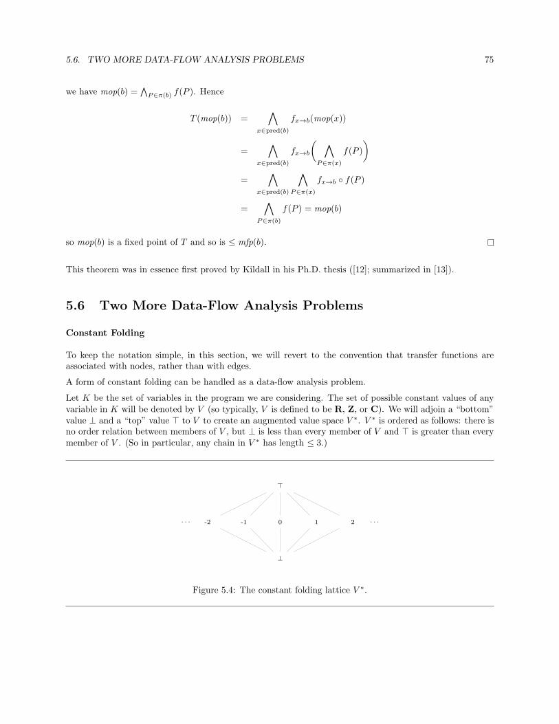
5.6. TWO MORE DATA-FLOW ANALYSIS PROBLEMS 75
we have mop(b) =∧
P∈π(b) f(P ). Hence
T (mop(b)) =∧
x∈pred(b)
fx→b(mop(x))
=∧
x∈pred(b)
fx→b
( ∧
P∈π(x)
f(P )
)
=∧
x∈pred(b)
∧
P∈π(x)
fx→b ◦ f(P )
=∧
P∈π(b)
f(P ) = mop(b)
so mop(b) is a fixed point of T and so is ≤ mfp(b).
This theorem was in essence first proved by Kildall in his Ph.D. thesis ([12]; summarized in [13]).
5.6 Two More Data-Flow Analysis Problems
Constant Folding
To keep the notation simple, in this section, we will revert to the convention that transfer functions areassociated with nodes, rather than with edges.
A form of constant folding can be handled as a data-flow analysis problem.
Let K be the set of variables in the program we are considering. The set of possible constant values of anyvariable in K will be denoted by V (so typically, V is defined to be R, Z, or C). We will adjoin a “bottom”value ⊥ and a “top” value ⊤ to V to create an augmented value space V ∗. V ∗ is ordered as follows: there isno order relation between members of V , but ⊥ is less than every member of V and ⊤ is greater than everymember of V . (So in particular, any chain in V ∗ has length ≤ 3.)
. . . -2 -1 0 1 2 . . .
⊥
⊤
Figure 5.4: The constant folding lattice V ∗.
76 CHAPTER 5. APPLICATIONS TO DATA-FLOW ANALYSIS
The semi-lattice L will consist of all functions from K to V ∗. L will be ordered in the obvious way pointwise(using the ordering of V ∗ defined above). 0 is just the function which is ⊥ everywhere, and 1 is the functionwhich is ⊤ everywhere. L has infinitely many elements. However, since there are finitely many variables inthe program—n, say—the length of any chain of elements in L is ≤ 2n+ 1; and hence L satisfies DCC, andin particular is complete.
The intuition for this is that if φ is a solution of our data-flow analysis problem, and if x is a variable in theprogram, then φ(x) has a value in V iff x is known to be constant, and the value of φ(x) is that constant.
φ(x) = ⊥ will mean that the variable x is not constant. φ(x) = ⊤ will mean that nothing is known aboutx—this happens only during the course of the algorithm; when the algorithm is finished the value ⊤ willnever occur. (The idea is that the value of φ at each local variable will be initialized to ⊤; clearly it would
be a semantic violation to use such a variable prior to assigning to it.)
Thus, every statement s in the program will have a function fs ∈ F associated with it, and the transfer func-tion for a basic block will be the functional composition of those functions corresponding to the statementsin that block. fs will be the identity function unless s is an assignment statement of one of the followingforms (where x and yj denote variables in the program):
x← a where a is a constant. Then fs is defined by
fs(φ)(w) =
{φ(w) if w 6= xa if w = x
x← θ(y1, . . . , yn) where the right-hand side is an expression involving only the variables y1, . . . , yn andpossibly some constants. Then fs is defined by
fs(φ)(w) =
φ(w) if w 6= x; and otherwise,θ(φ(y1), . . . , φ(yn)) if all φ(yj) are in V⊥ if any φ(yj) = ⊥
We don’t have to bother considering what happens when any φ(yj) = ⊤, since as we noted above, this
would be semantically invalid.
We let F be the set of functions generated by the identity and these functions and closed under functionalcomposition. To show that 〈L,∧,F〉 is a monotone data-flow analysis framework, it will be enough to showthat each of these generating functions is monotonic.
Suppose then that φ ≤ ψ are members of L. First, say s is a statement of the form x← a. Then we have
fs(φ)(w) = φ(w) ≤ ψ(w) = fs(ψ)(w)
if w 6= x, and they are equal if w = x; hence fs is monotonic.
Next, say s is a statement of the form x ← θ(y1, . . . , yn). If w 6= x then as before, fs(φ)(w) ≤ fs(ψ)(w).
Otherwise, w = x. Now if any of the φ(yj) = ⊥, then fs(φ)(w) = ⊥ ≤ fs(ψ)(w). Otherwise, none of the
φ(yj) = ⊥ and therefore none of the ψ(yj) = ⊥. As we noted before, we can assume that all φ(yj) and ψ(yj)
are in V . But then since each φ(yj) ≤ ψ(yj), we must have φ(yj) = ψ(yj) for all j, so fs(φ)(w) = fs(ψ)(w).
Thus 〈L,∧,F〉 is a monotone data-flow analysis framework. It is not, however, distributive, as the programin Figure 5.5 shows.

5.6. TWO MORE DATA-FLOW ANALYSIS PROBLEMS 77
x← 2
y ← 3
φ1 :
x → 2y → 3z → ⊤
x← 3
y ← 2
φ2 :
x → 3y → 2z → ⊤
z ← x+ y
φ3 :
x → ⊥y → ⊥z → ?
Figure 5.5: Non-Distributivity for Constant Folding
In this figure, φ1 ∧φ2 is ⊥ at both x and y and ⊤ at z. Hence, fz←x+y(φ1 ∧φ2)(z) = ⊥. On the other hand,
fz←x+y(φ1)(z) = fz←x+y(φ2)(z) = 5, so fz←x+y(φ1 ∧ φ2) 6= fz←x+y(φ1)∧ fz←x+y(φ2); i.e. the framework is
not distributive.
Finding Dominators
The problem of finding dominators in a flow graph can be cast into the form of a distributive data-flowanalysis problem, as follows:
Given a flow graph 〈G, s, e〉, the lattice L will consist of the set of all subsets of G, ordered by inclusion. In
particular, 0 = ∅, and 1 = G. The function fn corresponding to a node n ∈ G will be
fn(S) = S ∪ {n}.
where S is any subset of G.
It is easy to see that functions of this form (together with the identity function) constitute a distributive

78 CHAPTER 5. APPLICATIONS TO DATA-FLOW ANALYSIS
data-flow analysis framework. It is then obvious that the meet-over-paths solution (with the boundary value
condition Ss = {s}) yields precisely the set of dominators at each node, since it consists of those nodes whichoccur on every path from s to that node.
This gives us a reasonably good way of finding dominators in directed graphs. And although it is not themost efficient way, it is surely the simplest one conceptually.
Also, if we make the lattice meet operation ∧ correspond to ∪ instead of ∩, then the same data-flow analysisproblem, instead of yielding all the dominators of a node, yields all the “ancestors” of the node (with respect
to the whole graph; that is, all the nodes from which there is a path to the node under consideration).
5.7 How Many Iterations are Needed?
Many data-flow analysis frameworks have a property which enables us to show that the iterative AlgorithmE for finding mfp will converge quickly. There are various forms of this property, but they all say in oneform or another that in finding the mop solution to a data-flow problem, we can restrict ourselves to a finitenumber of paths.
Let us relax our assumption that all paths start at the entry node s of G. In general, our iterative algorithmsstart with an initial value α(x) ∈ L at each node x ∈ G, where α(s) = λ and otherwise α(x) = 1; for a path
P : x0 → x1 → . . .→ xn,
we define
f(P ) = fxn−1→xn◦ fxn−2→xn−1
◦ . . . ◦ fx1→x0(α(x0)).
Now each P ∈ π(b) either starts at s or can be extended to a path from s to b: say it does not start at s andthe new path is
P ′ : s = y0 → y1 → . . .→ ym = x0 → x1 → . . .→ xn = b.
Let us write
Q : s = y0 → y1 → . . .→ ym = x0.
Then we have f(Q) ≤ 1 = α(x0), and so f(P ) ≥ f(P ′).
Thus, adding all these new paths (the ones not starting at s) to the meet in computing mop cannot change
the value of mop, since each such new path is bounded below by a path already in the meet (i.e., already
starting at s).
Now suppose it is actually true that a finite number of paths suffices to compute mop; in fact, say we happento know that for each b ∈ G
mop(b) =∧
P∈π(b)
f(P )
where π(b) denotes some finite set of paths ending at b. (Note that this is a new and different use of the
notation π(b); the paths do not need to start at s.)

5.7. HOW MANY ITERATIONS ARE NEEDED? 79
By what we just saw above, if the path P is an element of π(b) and {Qi} is a finite set of paths such that∧f(Qi) ≤ f(P ), then P can be replaced in π(b) by {Qi}.
In Algorithm E (page 72), there is a choice made in the order in which the nodes are visited in the main
loop. Let us fix such an order once and for all. (We will later see that there is a natural order to use.)
Let us modify Algorithm E to produce Algorithm F in Figure 5.6. Given a particular path
P : x0 → x1 → . . .→ xn,
Algorithm F computes f(P ). By comparing Algorithm E with Algorithm F, we see that if Algorithm F
computes f(P ) in n(P ) iterations of the while loop, then after n(P ) iterations of the while loop in Algorithm
E, we must have m(b) ≤ f(P ).
beginm(s)← λ;for each node x ∈ G− {s} do
m(x)← 1;end for;
j ← 2;while j ≤ |P | do
for each b ∈ G− {s} doif (b = xj) then
m(xj)← fxj−1→xj(m(xj−1));
j ← j + 1;end if ;
end for;
end while;end
Figure 5.6: Algorithm F
Modified Algorithm E; Computes f(P )
Thus, if for each b ∈ G there is a finite set π(b) of paths ending at b (and not necessarily starting at s) suchthat
mop(b) =∧
P∈π(b)
f(P )
and if N is the maximum number of iterations of the while loop in Algorithm F to compute f(P ) for all
P ∈ ∪π(b), then after N iterations of the while loop in Algorithm E, we have
m(b) ≤∧
P∈π(b)
f(P ) = mop(b)
for all b ∈ G, and therefore Algorithm E can be stopped after N iterations. (If in fact, the data-flow problem
is distributive, then after N iterations, mfp(b) ≤ m(b) ≤ mop(b) = mfp(b), so Algorithm E actually ends
after N iterations.)
80 CHAPTER 5. APPLICATIONS TO DATA-FLOW ANALYSIS
There is a useful class of data-flow problems for which a finite number of paths suffices to compute mop;this is the class of problems for which mop can be computed solely in terms of the simple paths. Since everyflow graph is finite, there are only finitely many simple paths, and the analysis we have given above applies.
How can we characterize such data-flow problems? First, some notation: let us denote the sub-path fromsome node xj to another node xi of the path
P : x0 → x1 → . . .→ xn,
by xj∗→ xi, and let us write f
xj∗
→xifor
fxi−1→xi◦ fxi−2→xi−1
◦ . . . ◦ fxj→xj+1.
Thus, we have
f(P ) = fx0
∗
→xn(α(x0)) = f
xk∗
→xn◦ f
x0∗
→xk(α(x0))
The mop solution is the meet of f(P ) over all such paths P which start at s. If xk = xn (so the path has a
cycle in it), then we would like to split the path into two paths, eliminating a cycle in the process; we willshow below how to do this.
So suppose the path x0∗→ xn is split into x0
∗→ xk and xk
∗→ xn. We would like the expression for f(P ) to
be an upper bound for
fxk
∗
→xn(α(xk)) ∧ fx0
∗
→xk(α(x0)).
(If this is true, then as we have seen above, we can replace the path P by the two paths x0∗→ xk and
xk∗→ xn in computing mop.)
In particular, we want
f ◦ g(λ) ≥ f(1) ∧ g(λ)
for all f and g in F . Equivalently, setting x = g(λ), we want
(2) f(x) ≥ f(1) ∧ x.
It turns out that for distributive frameworks, this condition is sufficient:
5.11 Theorem If 〈L,∧,F〉 is a distributive framework satisfying (2), then the mop solution of any instance of
the framework can be found by forming the meet of f(P ) over all cycle-free paths.
Proof. Let
P : s = x0 → x1 → . . .→ xn = b
be a path from s to b which contains at least one cycle. Let j be the highest number such that xj equals
some xk with k > j. Then x0∗→ xj+1 and xj+1
∗→ xn together contain at least one less cycle than the

5.7. HOW MANY ITERATIONS ARE NEEDED? 81
original path, and the second path is actually simple. We have
f(P ) = fxj+1
∗
→xn◦ f
x0∗
→xj+1(λ)
≥ fxj+1
∗
→xn(1) ∧ f
x0∗
→xj+1(λ)
Hence we can replace any P : s∗→ b which contains a cycle by a finite set of paths each of which has fewer
cycles than P . By iterating this process, we can ultimately replace P by a finite set of cycle-free paths, andso mop(b) can be computed entirely in terms of cycle-free paths to b.
Since there are only finitely many cycle-free paths, we see that for a distributive data-flow framework satis-fying (2), mop can be calculated in terms of a finite number of paths. In fact, in this case, we can do evenbetter, provided the graph is reducible.
For reducible graphs, the loop-connectedness number (see page 39) lc(G) is ≤ dsl(G), where dsl(G) is thederived sequence length of G, and in general is ≤ 3. Now suppose that in Algorithm F above, we walk eachiteration of the nodes (in the while loop) in reverse postorder. Since for each path P , the nodes occur in
reverse postorder except for the back arcs in P , we see that it will take at most lc(G) + 1 iterations of the
while loop for algorithm F to compute f(P ) provided P is simple. (That is, it will take 1 iteration to reach
the first back arc, and 1 more iteration to get past that arc and reach the next one, or the end of the path.)
For instance, if a path in some graph has the form
2→ 3→ 6→ 16→ 17→ 20→ 30→ 12→ 32→ 40→ 5→ 9→ 19
where the numbers are the reverse post-order numbers of the nodes in the path, then on the first iterationof the while loop in Algorithm F, nodes 2 through 30 will be visited. (The first back arc is 30→ 12.) On the
next iteration, nodes 12 to 40 will be visited (up to the back arc 40 → 5). And then on the third iteration
of the while loop, nodes 5 through 19 will be visited and f(P ) will have been computed. Here there are 2
back arcs in P , and it took 3 executions of the while loop to compute f(P ).
To sum up, for distributive data-flow problems satisfying (2), Algorithm E needs only lc(G) + 1 iterations
of the while loop to compute mop. Of course, if we don’t know lc(G), then we will need an extra iteration
to confirm the “no change” test on the while loop, making the number of iterations lc(G) + 2. This result is
due to Kam and Ullman[9].
Data-flow frameworks where the L is a semi-lattice of boolean arrays (or, equivalently, of sets), and wherethe functions f ∈ F are of the form
f(x) = (x ∩ a) ∪ b
are called bit-vector frameworks , because they are implemented using bit vectors.
5.12 Theorem (Hecht and Ullman[7]) The while loop in Algorithm E is entered at most lc(G) + 2 times forbit-vector data-flow problems on reducible flow graphs, provided the nodes are visited in reverse postorder.
Proof. All we have to show is that the family of functions of the form
f(x) = (x ∩ a) ∪ b
82 CHAPTER 5. APPLICATIONS TO DATA-FLOW ANALYSIS
satisfies (2). But
f(x) = (x ∩ a) ∪ b
⊇ (x ∩ a) ∪ (x ∩ b)
= x ∩ (a ∪ b)
= x ∩ f(1)
Thus, the natural way to visit the nodes in Algorithm E is in reverse post-order; and if the graph is reducible,then we can actually get an effective bound on the running time of the algorithm when applied to bit-vectorproblems.
This kind of analysis can be extended to data-flow frameworks for which mop can be computed by consideringpaths containing at most k cycles. Again, the conditions only apply to distributive frameworks. Frameworkssuch as these are sometimes called fast frameworks . See for instance Tarjan’s papers [21], [23], and [22].
More general conditions, not requiring distributivity, have also been considered by Graham and Wegman [4]
and Rosen [15]. These conditions do not yield an efficient algorithm for mop 4; but they do yield an efficientalgorithm which computes a solution which is guaranteed to be between mfp and mop. These conditions,however, are not broad enough to include the problem of constant propagation considered earlier.
5.8 Algorithms Based on Reducibility
The algorithm we have been using up to this point consists of iterating over all the nodes of G a certainnumber of times. For this reason, it is called the iterative algorithm. For bit-vectoring problems where theflow graph is known to be reducible, there are some algorithms which potentially can save execution time,at the cost of managing more complicated data structures.
We will consider two such algorithms here. Both algorithms take their most natural form for reduciblegraphs, but both can be extended to apply to general flow graphs. Let us start, however, by assuming thatG is reducible. Both these algorithms lean heavily on the fact that we can restrict ourselves to cycle-freepaths when computing the data-flow solutions.
Since the algorithms are based on the derived sequence of a reducible flow graph, we cannot consider backwarddata-flow problems to be forward problems on the reverse flow graph—as we noted previously, the reversegraph of a reducible flow graph is not necessarily reducible. Thus separate algorithms are necessary forforward and backward problems.
Given a path Q in G of the form
Q : q0 → q1 → . . .→ qs,
let us write
fQ = fqs−1→qs ◦ fqs−2→qs−1◦ . . . ◦ fq0→q1 .
The algorithms will be based on the following lemma:
4In a negative direction, Kam and Ullman [10] have shown that there is no general algorithm which computes mop for allnon-distributive problems.

5.8. ALGORITHMS BASED ON REDUCIBILITY 83
5.13 Lemma Let 〈L,∧,F〉 and 〈G, s〉 be an instance of a distributive data-flow analysis framework satisfying
DCC and (2). If all simple paths from s to x in G pass through a node k, then
mop(x) =
( ∧
paths Q fromk to x
fQ
)(mop(k)).
Proof. Each simple path P from s to x corresponds uniquely to a pair of paths R from s to k, and Q fromk to x, by the composition “P is R followed by Q”; and conversely. Correspondingly, we have fP = fQ ◦ fR.
Hence by Lemma 5.8,
mop(x) =∧
paths P froms to x
fP (λ)
=∧
paths Q fromk to x
∧
paths R froms to k
fQ ◦ fR(λ)
=∧
paths Q fromk to x
fQ
( ∧
paths R froms to k
fR(λ)
)
=∧
paths Q fromk to x
fQ(mop(k))
=
( ∧
paths Q fromk to x
fQ
)(mop(k))
5.8.1 Allen and Cocke’s Algorithm
This algorithm is essentially that presented in Allen and Cocke[3], although the notation is closer to thatused in the Schwartz and Sharir algorithm, which we present subsequently.
G = G0, G1, . . . , Gn = {g}
will be the derived sequence of G. The function φj will map each interval of Gj to its corresponding point in
Gj+1. The function hj , applied to an interval in Gj , returns the element of Gj which is the header of that
interval.
Let us also define a function θj : Gj → G as follows: θ0 is just the identity function on G. If j ≥ 1, then
θj(x) is that element of G which represents the “ultimate header” of x. (For instance, in the example of
Figure 3.11 on page 42, θ3(C3) = C.) Formally, we can define θj recursively as follows:
θj(x) =
{x j = 0θj−1hj−1φ
−1j (x) j > 0
84 CHAPTER 5. APPLICATIONS TO DATA-FLOW ANALYSIS
The functions fx→y are assumed to have already been computed, and are denoted as f0(x, y).
These functions may seem complicated. The point to keep in mind is that they really come for free—theyjust represent the information in the data structure representing the flow graph and its derived sequence.
Let us make the convention that P is a path in Gj of the form
P : po → p1 → . . .→ pr
and Q is a path in G of the form
Q : q0 → q1 → . . .→ qs.
ι will represent the identity function on the semi-lattice L.
The Forward Algorithm
The algorithm consists of two passes over the derived sequence. In the first pass, which proceeds from innerto outer intervals (that is, from G0 to Gn), we compute at each stage (that is for each Gj) three sets of
functions:
• For each arc x→ y in Gj , fj(x, y), which will be computed recursively from the computations in Gj−1,
will represent data flow from θj(x) to θj(y):
fj(x, y) =∧
paths Q fromθj(x) to θj(y)
fqs−1→qs ◦ fqs−2→qs−1◦ . . . ◦ fq0→q1
(where q0 = θj(x) and qs = θj(y)).
• For each interval 〈K, k〉 in Gj and each x ∈ K, gj(x) is the function which represents data flow from
k to x within K:
gj(x) =∧
paths P fromk to x
fj(pr−1, pr) ◦ fj(pr−2, pr−1) ◦ . . . ◦ fj(p0, p1)
=∧
paths Q fromθj(k) to θj(x)
fqs−1→qs ◦ fqs−2→qs−1◦ . . . ◦ fq0→q1
(where again q0 = θj(x) and qs = θj(y) and where p0 = k and pr = y.)
Thus for all x ∈ K,
gj(x) =∧
y∈predj(x)y∈K
fj(y, x) ◦ gj(y).
5.8. ALGORITHMS BASED ON REDUCIBILITY 85
• For each successor x of K, Fj(K,x) is the function which represents data flow from k through K andout to x:
Fj(K,x) =∧
y∈predj(x)y∈K
fj(y, x) ◦ gj(x).
Fj will then be reinterpreted as fj+1 when Gj+1 is processed.
In computing gj(x), we can restrict ourselves to cycle-free paths from k to x. This means, since K is an
interval, that gj(x) can be computed in 1 pass over the nodes in K, except for paths with a back arc in
them. The only such paths end at k: if x = k, we compute gj(x) separately by a final meet over paths from
its predecessors.
The second pass over the derived sequence proceeds from outer to inner intervals. mn(g) is set equal to λ.
Then for each interval 〈K, k〉 in Gj , mj(k) is set equal to mj+1(φj(K)). Finally, for each x ∈ K, mj(x) is
set equal to gj(x)(mj(k)). By induction, we see that at each step of this pass, for each interval 〈K, k〉 in Gj ,
• mj(k) is set equal to the mop solution at θj(k).
• Then, since for each x ∈ K, any cycle-free path from s to θj(x) must pass once through θj(k),
Lemma 5.13 shows that mj(x) is set equal to the mop solution at θj(x).
Hence, at the end of the algorithm, which is in Figure 5.7, m0 is the solution to the data-flow problem.
The Backward Algorithm
The modification of the Allen-Cocke algorithm for backwards data-flow propagation is due to Kennedy. Hisversion, and the original references, can be found in [11].
The backwards problem is complicated by the fact that, although intervals are single-entry, they are notsingle-exit. Since we are following data-flow backwards through the flow graph, we have to take account ofthe fact that intervals can be entered at different points.
As usual, the exit node of the flow graph is denoted by e. Let us denote the image of e in Gj by ej (so in
particular, e0 = e and en = g). Further, let us adjoin a dummy “post-exit” node δj to each Gj , and a single
edge ej → δj . δj will not be thought of as being a member of Gj , and in particular, will not be a member
of any interval of Gj . Its only function is to be a technical help in the algorithm. We set fe0→δ0 ← ι.
Again we make two passes over the derived sequence. In the first pass, which again proceeds from inner toouter intervals, (that is, from G0 to Gn), we compute for each Gj three sets of functions:
• For each arc x→ y in Gj , fj(x, y), which will be computed recursively from the computations in Gj−1,
will represent data flow from θj(y) backwards to θj(x):
fj(x, y) =∧
paths Q fromθj(x) to θj(y)
fq0→q1 ◦ fq1→q2 ◦ . . . ◦ fqs−1→qs

86 CHAPTER 5. APPLICATIONS TO DATA-FLOW ANALYSIS
-- Step I: Inner-to-outer interval processing.
for j = 0 to n− 1 do
if j 6= 0 then-- f0 is already defined.
for each arc x→ y in Gj do
fj(x, y)← Fj−1(φ−1j (x), hj−1(φ
−1j (y)));
end for;end if ;for each interval 〈K, k〉 in Gj do/
for each x ∈ K do
initialize gj(x) to the constant function 1;end for;repeat
for each x ∈ K − {k} do
gj(x)←∧
y∈predj(x)y∈K
fj(y, x) ◦ gj(y);
end for;
until no change;
gj(k)←∧
y∈predj(k)y∈K
f(y, k) ◦ gj(y);
for each successor x of K do/
Fj(K,x)←∧
y∈predj(x)y∈K
fj(y, x) ◦ gj(y);
end for;end for;
end for;
-- Step II: Outer-to-inner interval processing.mn(g)← λ;for j = n− 1 to 0 step −1 do
for each interval 〈K, k〉 in Gj do-- mj+1 is known.mj(k)← mj+1(φj(K));for each x ∈ K − {k} do
mj(x)← gj(x)(mj(k));end for;
end for;
end for;
The repeat loop only has to be executed once provided the nodes in its for loop are visited inreverse post-order.
Figure 5.7: Allen and Cocke’s Algorithm: Forward Data-Flow Propagation
5.8. ALGORITHMS BASED ON REDUCIBILITY 87
(where q0 = θj(x) and qs = θj(y). Note the order in which the functions are composed to form each
fQ—this is backwards propagation.)
• For each interval 〈K, k〉 in Gj , each x ∈ K, and each y ∈ succ(K), gj(x, y) represents the data flow
backwards from the beginning of y (i.e. from the exit of K to y) back through K to x:
gj(x, y) =∧
paths P fromx to y
fj(p0, p1) ◦ fj(p1, p2) ◦ . . . ◦ fj(pr−1, pr)
=∧
paths Q fromθj(x) to θj(y)
fq0→q1 ◦ fq1→q2 ◦ . . . ◦ fqs−1→qs
Thus for all x ∈ K,
gj(x, y) =∧
x→ww∈Kor w=y
fj(x,w) ◦ gj(w, y)
with the convention that gj(y, y) = ι.
• For each successor y of K,
Fj(K, y) = gj(k, y).
In computing gj(x, y), if we visit the nodes x in K in reverse post-order, then at most two passes over the
interval will be necessary, since any simple path from x to a successor y of K can contain at most one backarc (and this will be true iff the path contains the interval header k).
The second pass over the derived sequence proceeds from outer to inner intervals. We compute a functionγj : Gj → F . If x ∈ Gj , γj(x) will represent data flow backward from the exit e to θj(x) (that is, it will be
the meet of all functions fQ where Q runs over all paths from θj(x) to the exit).
γj is computed as follows: first, γn(g) is set equal to gn(g, δn). For each j (stepping down from n− 1 to 0),
for each interval 〈K, k〉 in Gj , we first set γj(k) to be γj+1 of the image of K in Gj+1. Then again for each
interval 〈K, k〉 in Gj , and for each node x ∈ K − {k}, we set
γj(x)←∧
y∈succ(K)
gj(x, y) ◦ γj(y).
We see by induction that for each interval 〈K, k〉 of Gj ,
• γj(k) is the meet of all functions fQ where Q runs over all paths from θj(k) to the exit.
• Since for each x ∈ K, any cycle-free path from s to θj(x) must past once through θj(k), a minor variant
of Lemma 5.13 shows that γj(x) is the meet of all functions fQ where Q runs over all paths from θj(x)
to the exit.
88 CHAPTER 5. APPLICATIONS TO DATA-FLOW ANALYSIS
Hence, at the end of the algorithm, the mop solution will be m(x) = γ0(x)(λ) for all x ∈ G.
The complete algorithm is given in Figure 5.8.
Kennedy’s original algorithm did not use the fact that we knew gj(x, y) for all x ∈ K, and therefore computed γj as follows:
after first computing γj for each interval header in Gj as above, for each 〈K, k〉 in Gj , the nodes x ∈ K − {k} are visited in
post-order. For each such node x, we set
γj(x)←∧
y∈succ(x)
{
fj(x, y) ◦ γj(y) if y ∈ K
gj(x, y) ◦ γj(y) otherwise
Since the nodes x ∈ K are visited in post-order, each y ∈ succ(x) has either
1. been visited already in the interval; or
2. is the target of a back arc in the interval, in which case it is the interval header; or
3. is the target of an arc to another interval, in which case it is the header of another interval.
In each case, γj(y) has already been assigned. Thus, one pass through each interval computes γj .
5.8.2 Schwartz and Sharir’s Algorithm
One inefficiency in the algorithms as just presented, is that there may be nodes in one of the derived graphswhich are unaffected by the next reduction, and so remain in the next derived graph. (See, for instance,
Figure 3.10 on page 41.) Certainly there is no reason to visit these intervals again.
Schwartz and Sharir [16] noticed that the tree of reachunder sets created by Tarjan’s algorithm for testingreducibility could be used instead of the tree reflecting the nesting of intervals of all orders to obtain a moreefficient algorithm.
So instead of dealing with the derived sequence of G, we will deal with the sequence {ρj = ρj(kj) : 1 ≤ j ≤ n}
defined as follows: For 1 ≤ j < n, ρj is the jth reachunder set produced by Tarjan’s algorithm, and ρn is the
limit graph produced by the algorithm. (Since G is assumed to be reducible, ρn is a DAG.) In each case, kjis the header of ρj .
When a reachunder set ρj is identified by Tarjan’s algorithm, it is collapsed into a point pj , which becomes
an element of the next set ρj+1. Instead of separate functions fj , we will have one function f(x, y), where x
and y may be points in G or elements pj , as appropriate. The forward algorithm is given in Figure 5.9.
For the backward algorithm, we only need one additional node δ, which, since it is not part of any reachunderset (or in fact, part of G), is never collapsed into any of the points {pj}. We set f(e, δ)← ι.
The backward algorithm is given in Figure 5.10.
5.8.3 Dealing With Non-Reducible Flow Graphs
The Schwartz-Sharir algorithm can be easily modified to handle non-reducible flow graphs, as follows: Duringthe computation of reachunder sets in Tarjan’s algorithm, the nodes kj which are targets of back arcs are
visited in reverse pre-order. If the reachunder set of kj includes s (so we know that G is not reducible), then
no action is taken other than marking kj as “improper”. Then the set kj+1 is computed as usual, and the
algorithm proceeds. If any ρn contains an “improper” node, it is also marked as “improper”.

5.8. ALGORITHMS BASED ON REDUCIBILITY 89
-- Step I: Inner-to-outer interval processing.for j = 0 to n− 1 do
if j 6= 1 then
-- f1 is already defined.for each arc x→ y in Gj do
fj(x, y)← Fj−1(φ−1j (x), hj−1(φ
−1j (y)));
end for;fj(ej , δj)← ι;
end if ;for each interval 〈K, k〉 in Gj do
for each x ∈ K and y ∈ succ(K) do/Initialize gj(x, y) to the constant function 1;Initialize gj(y, y) to ι;
end for;
repeatfor each x ∈ K do
gj(x, y)←∧
x→ww∈K or w=y
fj(x,w) ◦ gj(w, y);
end for;until no change;
for each successor y of K doFj(K, y)← gj(k, y);
end for;
end for;end for;
-- Step II: Outer-to-inner interval processing.γn(g)← gn(g, δn);for j = n− 1 to 0 step −1 do
for each interval 〈K, k〉 in Gj doγj(k)← γj+1(φj(K));
end for;for each interval 〈K, k〉 in Gj do
for each x ∈ K − {k} do
γj(x)←∧
y∈succ(K)
gj(x, y) ◦ γj(y);
end for;
end for;
end for;
-- Step III: Final propagation step.for each x ∈ G do
m(x)← γ0(x)(λ);end for;
The repeat loop only has to be executed twice provided the nodes in its for loop are visited inreverse post-order.
Figure 5.8: Allen and Cocke’s Algorithm: Backward Data-Flow Propagation

90 CHAPTER 5. APPLICATIONS TO DATA-FLOW ANALYSIS
-- Step I: Inner-to-outer interval processing.
for j = 0 to n− 1 do
for each x ∈ ρj doinitialize gj(x) to the constant function 1;
end for;
repeatfor each x ∈ ρj − {kj} do
gj(x)←∧
y∈predj(x)y∈K
f(y, x) ◦ gj(y);
end for;
until no change;
gj(kj)←∧
y∈predj(k)y∈ρj
f(y, kj) ◦ gj(y);
for each successor x of ρj do
f(pj , x)←∧
y∈predj(x)y∈ρj
f(y, x) ◦ gj(y);
end for;
for each predecessor x of ρj dof(x, pj)← f(x, kj);
end for;
end for;
-- Step II: Outer-to-inner interval processing.mn(pn)← λ;for j = n− 1 to 0 step −1 do
-- mj+1 is known.mj(kj)← mj+1(pj);for each x ∈ ρj − {kj} do
mj(x)← gj(x)(mj(kj));end for;
end for;
If G is reducible, the repeat loop only has to be executed once provided the nodes in its for loopare visited in reverse post-order.
Figure 5.9: Schwartz and Sharir’s Algorithm: Forward Data-Flow Propagation

5.8. ALGORITHMS BASED ON REDUCIBILITY 91
-- Step I: Inner-to-outer interval processing.for j = 0 to n− 1 do
for each x ∈ ρj and y ∈ succ(ρj) doInitialize gj(x, y) to the constant function 1;Initialize gj(y, y) to ι;
end for;
repeatfor each x ∈ K do/
gj(x, y)←∧
x→ww∈K or w=y
f(x,w) ◦ gj(w, y);
end for;
until no change;
for each successor y of ρj dof(pj , y)← gj(k, y);
end for;
for each predecessor x of ρj dof(x, pj)← f(x, kj);
end for;
end for;
-- Step II: Outer-to-inner interval processing.γn(g)← gn(g, δ);for j = n− 1 to 0 step −1 do
γj(kj)← γj+1(pj);for each x ∈ ρj − {kj} do
γj(x)←∧
y∈succ(ρj)
gj(x, y) ◦ γj(y);
end for;end for;
-- Step III: Final propagation step.
for each x ∈ G do
m(x)← γ0(x)(λ);end for;
If G is reducible, the repeat loop only has to be executed twice provided the nodes in its for loopare visited in reverse post-order; and when j = n, it only has to be executed once (since ρn isknown to be a DAG).
Figure 5.10: Schwartz and Sharir’s Algorithm: Backward Data-Flow Propagation

92 CHAPTER 5. APPLICATIONS TO DATA-FLOW ANALYSIS
The only change in the algorithms then that has to be made is that in Step I of each, the repeat loop for animproper ρj really has to be repeated until no change. That is, improper reachunder sets (or an improper
terminal DAG) are handled by the iterative algorithm.

Bibliography
[1] Alfred V. Aho, John Hopcroft, and Jeffrey D. Ullman. Data Structures and Algorithms. Addison-Wesley,Reading, Massachusetts, 1983.
[2] Alfred V. Aho, Ravi Sethi, and Jeffrey D. Ullman. Code optimization and finite Church-Rosser sys-tems. In Randall Rustin, editor, Design and Optimization of Compilers, pages 89–106. Prentice-Hall,Englewood Cliffs, New Jersey, 1971.
[3] F. E. Allen and John Cocke. A program data flow analysis procedure. Communications of the ACM,
19(3):137–147, 1976.
[4] Susan L. Graham and Mark Wegman. A fast and usually linear algorithm for global flow analysis.
Journal of the ACM, 23(1):172–202, January 1976.
[5] Matthew S. Hecht. Flow Analysis of Computer Programs. North-Holland, New York, 1977.
[6] Matthew S. Hecht and Jeffrey D. Ullman. Flow graph reducibility. SIAM Journal on Computing,
1(2):188–202, June 1972.
[7] Matthew S. Hecht and Jeffrey D. Ullman. Analysis of a simple algorithm for global flow problems.In Conference Record of the First Annual ACM Symposium on Principles of Programming Languages,Boston (Mass.), pages 207–217, October 1973.
[8] Matthew S. Hecht and Jeffrey D. Ullman. Characterizations of reducible flow graphs. Journal of the
ACM, 21(3):367–375, July 1974.
[9] John B. Kam and Jeffrey D. Ullman. Global data flow analysis and iterative algorithms. Journal of the
ACM, 23(1):158–171, January 1976.
[10] John B. Kam and Jeffrey D. Ullman. Monotone data flow analysis frameworks. Acta Informatica,
7(3):305–317, 1977.
[11] Ken Kennedy. A Survey of Data Flow Analysis Techniques. In Steven S. Muchnick and Neil D. Jones,editors, Program Flow Analysis: Theory and Applications, pages 5–54. Prentice-Hall, Englewood Cliffs,New Jersey, 1981.
[12] Gary Arlen Kildall. Global Expression Optimization During Compilation. PhD thesis, University ofWashington, Seattle, Washington, May 1972.
93
94 BIBLIOGRAPHY
[13] Gary Arlen Kildall. Global expression optimization during compilation. In Conference Record of the
First Annual ACM Symposium on Principles of Programming Languages, Boston (Mass.), pages 194–206, October 1973.
[14] Donald Knuth. An empirical study of FORTRAN programs. Software Practice and Experience,
1(12):105–134, 1974.
[15] Barry K. Rosen. Monoids for rapid data flow analysis. SIAM Journal on Computing, 9(1):159–196,1980.
[16] J. T. Schwartz and M. Sharir. A design for optimizations of the bitvectoring class. Technical Report 17,Courant Institute of Mathematical Sciences, Computer Science Department, September 1979.
[17] M. Sharir. A strong-connectivity algorithm and its applications in data flow analysis. Computation and
Mathematics with Applications, 7(1):67–72, 1981.
[18] M. Sharir. Structural analysis: A new approach to flow analysis in optimizing compilers. Computer
Languages, 5(3/4):141–153, 1981.
[19] Robert Endre Tarjan. Finding dominators in directed graphs. SIAM Journal on Computing, 3(1):62–89,1974.
[20] Robert Endre Tarjan. Testing flow graph reducibility. J. Computer and System Sciences, 9:355–365,1974.
[21] Robert Endre Tarjan. Iterative algorithms for global flow analysis. In J. F. Traub, editor, Algorithmsand Complexity: New Directions and Recent Results, pages 71–102. Academic Press, 1976.
[22] Robert Endre Tarjan. Fast algorithms for solving path problems. Journal of the ACM, 28(3):594–614,1981.
[23] Robert Endre Tarjan. A unified approach to path problems. Journal of the ACM, 28(3):577–593, 1981.
[24] Alfred Tarski. A lattice-theoretical fixpoint theorem and its applications. Pacific Journal of Mathemat-ics, 5:285–309, 1955.

Index
ancestor, 2, 19arc
back, 3cross, 4forward, 3tree, 3
available expression, 59
backward equations, 63boundary value equations, 62
chain, 45height, 45
child, 2, 19collapsing a flow graph, 47confluence equations, 63consumes, 47cycle, 19cycle-free, 19
data flow analysis frameworkmonotone, 69
data-flow problemdistributive, 65monotone, 69
derived sequence, 29derived sequence length, 39descendant, 2, 19descending chain condition, 72distributive, 73dominator, 20
immediate, 21strong, 20
dominator tree, 21dsl, see derived sequence length
entry node, 24
finite Church-Rosser transformation, 45
finite relation, 45flow graph, 19
derived, 28kernel, 51limit, 29reverse, 59trivial, 19
forward equations, 63framework
bit-vector, 81fast, 82monotone, 69
functiondistributive, 65monotonic, 68
head, 1header, 24
interior, 19interval, 24interval nesting, 40interval nesting tree, 42irreducible, 29
kernel, 51
lattice, 68lc, see loop-connectedness numberlimit point, 45live variable, 60loop, 19loop-connectedness number, 39lower semi-lattice, 67
complete, 68
maximal fixed-point solution, 72meet-over-paths solution, 70mfp, see maximal fixed-point solution
95
96 INDEX
monotone data flow analysis frameworkinstance, 70
mop, see meet-over-paths solution
nonreducible, 29
Path Lemma, 11pre-interval, 24predecessor, 2, 19propagation equations, 63
reaching definition, 60reachunder set, 53reducible, 29reduction ordering, 56region, 24reverse graph, 12root of a strongly connected component, 13
self-loop, 19simple, 19source, 1successor, 2, 19
tail, 1target, 1transfer equations, 63
very busy expression, 61