notes on infrared absorption experiments in a methane molecular beam
TRANSCRIPT

NBSlR 73-312
NOTES ON INFRARED ABSORPTION EXPERIMENTS IN A METHANE MOLECULAR BEAM
P. Kartaschoff Stephen Jarvis, Jr.
Time and Frequency Division Inst i tu te for Basic Standards National Bureau o f Standards Boulder, Colorado 80302
May 1973
US. DEPARTMENT OF COMMERCE, Frederick 6. Dent, Secretary# !So
NATIONAL BUREAU OF S T A N D A R D S . Richard W Roberts. Director
Contents
Page
1. INTRODUCTION . . . . . . . . . . . . . . . . . . . 2
2. ABSORPTION IN SINGLE STANDING WAVE- OPTICAL BEAM . . . . . . . . . . . . . . . . . . . 4
3. DISCUSSION O F MULTIPLE OPTICAL BEAM EXCITATION.. . . . . . . . . . . . . . . . . . . . 9
4. REFERENCES . . . . . . . . . . . . . . . . . . . 15
APPENDIX A . . . . . . . . . . . . . . . . . . . . . . . 16
APPENDIX B . . . . . . . . . . . . . . . . . . . . . . . 22
iii

LIST O F FIGUR-ES Page
Figure 1. Geometry of molecular beam-optical wave interaction . . . . . . . . . . . . . . . . . . . . . 3
Figure 2 . Phase p of individual trajectory . . . . . . . . . . . 5
Figure 3. Approximate transition probability for individual trajectory with Doppler shift cc: 8
0 ” ” ” ” ” ’
Figure 4. Schematic of three-field separated cavity system . . . . . . . . . . . . . . . . . . . . . . 12
iv

NOTES ON INFRARED ABSORPTION EXPERIMENTS IN A METHANE MOLECULAR BEAM*
P. Kartaschoff 7 Laboratoire Suisse de Recherches Horloggres
Neuc hgtel, Switz e rland
and
Stephen Jarvis, Jr. Time and Frequency Division National Bureau of Standards
Boulder, Colorado USA
The problem of calculating the transition probability of methane molecules in a molecular beam interacting with an infrared (3 . 39p) radiation beam is discussed. Contrary to the usual microwave molecular beam experiments, f irst- order Doppler frequency shifts cannot be neglected. This makes the solution of the wave-equations more difficult. Weak field approximations to the transition probability have been calculated. to the Rabi-type interaction result in a Doppler-broadened absorption line with an estimated half-power width of a few MHz. For separated multiple field experiments analogous to the Ramsey-type interaction, no observable response i s predicted, the expected sharp resonance pattern being smeared out by the random Doppler shifts due to the spread of the molecular beam trajectories. Further investigations a r e required in order to predict the resonance line shapes for strong fields, i. e. , saturated absorption.
Single optical beam experiments analogous
Key Words: Frequency standard; methane resonance; molecular beam; Ramsey resonance; .
saturated absorption; stabilized l a se r ; transition probability .
:k Contribution of the National Bureau of Standards, not subject to
t P. Kartaschoff was a visiting scientist in the Time and Frequency copyright.
Division, Institute for Basic Standards, from October 1970 to September 1971. Centre Technique, 3000 Bern 29, Switzerland.
He i s now at Direction Generale des PTT,

1. INTRODUCTION
In 1970 H. Hellwig suggested a methane molecular beam
absorption experiment for the investigation of the photon recoil effect [ 1 J
which might limit the accuracy of the 3 . 39 - pm saturated absorption cell
frequency standard of R. Barger and J. Hall. This note summarizes
some f i r s t attempts to gain more understanding of the interactions
between the infrared radiation field and the molecular beam.
see that one of the main problems is the first order Doppler shift which
i s not negligible a t these short wavelengths.
different f rom that encountered in a microwave molecular beam
apparatus (e. g., cesium).
We shall
The situation i s very
We f i rs t note some initial data and facts:
a ) Dimensions of the interaction region
Optical beam diameter A = 0. 1 c m
Separation for Ramsey interaction L = 5 c m
Molecular Beam Dimensions: Width - 1 c m Height - 0. 1 c m
Divergence of molecular t ra jector ies c 0. 1 radian.
A compromise between divergence, which can be reduced by collimation,
and useful f l u x has to be made. Similarly to the absorption cell, selec-
tion of t ra jector ies is also possible by saturated absorption. However, .
we then have more problems in understanding the recoil effect.
b) State selection
The source temperature can be situated between 78K and 300K;
thus the ratio hv lies between 5 6 and 15 and the initial population of the
upper energy level of the transition can be neglected. kT
2

W e have v- = v , (1 + P 1
V where B = < ; , v being the velocity of the molecule and < <( 1 the 6,
angle
OPTICAL S T A N D I N G N A V E S
F i g u r e 1. Geometry of molecular beam-optical wave interaction.
between the molecule trajectory and the wavefront in the plane of the
trajectory. For methane, we have v - 3 X 10 c m s and thus with
6 = 10 c . An absorption experiment using a c = 3x10 c m s
traveling wave puts an unfulfillable requirement on the adjustment of
the optical and molecular beams with respect to each other, as
4 -1
-1 -6 10
-3 = 10 radian would shift the absorption line by its entire width.
The shift can be reduced or compensated by using a standing
wave produced by a Fabry-Perot cavity. We then have an interaction -
3

with two equal and opposite running waves.
but only a Doppler broadening due to the divergence of the beam,
assuming that we have indeed a pure standing wave.
will not be entirely perfect and this may limit the accuracy of the
e xp e r ime nt .
We thus expect no shift
Actual resonators
2 . ABSORPTION IN SINGLE STANDING WAVE OPTICAL BEAM
The following treatment is based on Ramsey's calculations of
the transition probability of a two-level system perturbed by a periodic
field [ 2, Section V. 3 1 . The form of the perturbation is different,
however, because we have to deal with two simultaneously applied
oscillating fields of equal amplitude but slightly different frequencies.
This case has not been treated in the ear l ie r l i terature on microwave
molecular beam spectroscopy because there i t was usually either
possible to neglect first order Doppler shifts o r if
simultaneous perturbations by two frequencies were considered, one
was assumed to be very much weaker than the other. We therefore
could not see how the older work could be used. If we look at the
geometry as shown in figure 2,
two running waves, which has to degenerate into the classical case
[ 3 ] - [ 6 ] ,
we have a perturbation by each of the
of Rabi for < = 0, i.e. for a molecular trajectory exactly paral le l to
the plane in which the nodes of the field pattern l ie.
4

Figure 2. Phase p of individual trajectory.
F o r the two-level system we have the wave function [ 2 3 , [7 ’J
q % $ ( t ) = C $ t c P P
as a solution of the wave equation
Since we have two equal amplitude waves running in opposite directions,
the perturbation takes the following form
i(u t uD)t Ab v = - ( e t e P 9 2
q P 2
- i ( w t wD)t e t e

which, by adding an initial phase angle p (see fig. Z ) , can also be
written as :
i o t V = h b e cos( .o t t p)
-iWt V = h b e cos(.w t t p)
Pq D
w D
where o is the Doppler shift (angular frequency) D
V o = ooP = oo& * D
With the assumed dimensions and velocity i t is easy to see that W t D o var ies between the limits :
a where t = - . form; after transformation a s in [ Z ] :
The wave equations to be solved take the following o v
d iot i - C ( t ) = W C ( t ) t b e cos((3Dt t p)Cq( t )
dt P P P
d - io t i - C ( t ) = b e cos(WDt t p)C ( t ) t W C ( t )
dt 9 P q q
where
P
a r e the energies of the two levels p and q, so that
w - w = x u . 9 P 0
The above equations a r e to be solved with the initial conditions
6

c ( 0 ) = 1 c ( 0 ) = 0 . (2) P q
It is easily verified that for 0 = 0 the case t reated by Ramsey is D obtained and the solution in closed form is obtained for the transition
probability 3 L
P = I C 1 . PI 9 9
Unfortunately, a closed form solution in our case has not been
found.
We have obtained the following approximate solutions using
the approach of Appendix A.
The solution depends on the phase angle p,
field where the molecule enters the field region (see fig. 2) and is
to be averaged over (0 , 2 T ) .
0 I p 5 27~ of the
For very small values of b t the solution is: (without higher 0
order te rms)
a o v with A = ( u o - W ) and t = - . This solution is valid for one
typical trajectory incidence a n le and is to be averaged over the
<, which again is not possible in possible values of 0 = - closed form but easily done on a computer.
WO D C
It is nevertheless possible to discuss this resu l t : sin x 2
WD We have a superposition of t e rms of the ( - ) type. Finite X
yields the following picture for a single trajectory :
7

u 0
Figure 3. Approximate transition probability for individual trajectory with Doppler shift w .
0 A finite spread in and w respectively smear s oat the la teral
wiggles and we obtain a simple Doppler-broadened central peak at LIJ
with a half width of about 2 aD
D
0 (rough estimate) i.e., for
max
-6 = 3 . 3 x 1 0 s a 0 . 1 t = - = 3 x l o 4 o v
6 7 -1 - - - 40 x10 = 1 . 2 x 1 0 s D 3 . 3
0
max
2 V b - - 3.8 MHz D = WD with 2 a v
as an estimate for the observed linewidth.
so that we obtain a line-Q of only about
This is very broad indeed,
13 ( V o = 8 . 8 X 1 0 H z ) . 7 2 x 10
As a conclusion, saturated absorption has to be attempted also in the
case of the molecular beam experiment. The possibility of a Ramsey
separated field excitation scheme has been discussed too.
moment, an attempt to solve the wave equation appears to be a rather
formidable task in the case of separated fields.' To compute the
F o r the
8

discussion of the single beam ("Rabi"-type) case, the following results
may be obtained:
a) Expressions valid for larger values of b t have been obtained, they
a r e asymptotic for b t - , but 0
0 1) they a r e singular at the resonance h = 0
2) they contain elliptic integrals.
b) At resonance X = 0 , the following expressions have been obtained:
s in wDto) 2b 2b
P D D A = 0
u t )
D O sin - 4b
- 2 Jo ( w 2 D
J o ( x ) being the Bessel-Function.
the range of W
c)
This is again to be averaged over
D ' Fo r a particle with zero Doppler shift we have
w = o , x = o D
The last expression allows, in principle, to estimate the required
power for saturated absorption.
3 . DISCUSSION OF MULTIPLE OPTICAL BEAM EXCITATION
At this stage, we can only discuss the weak-field approximations.
The result shown in the preceding section (fig. 3)
superposition of the two independent solutions of the Schrsdinger - Equation, with one single, Doppler -shifted perturbation applied each
time.
is equivalent to the
In other words, and this can easily be verified in [ 2 ] , we have

the sum of two shifted Rabi-type resonances, the shifts being + uD and
- W respectively. D ' It therefore seems reasonable to assume, without proof, that the
same should be t rue for Ramsey-type resonances produced by two or
more separated fields.
We shall see, however, that for this weak-field assumption,
the average result, i.e., averaged over the spread of incidence angles
(see fig. 2) vanishes. In an experiment, we can predict that only
the Doppler-broadened (A V - 3 MHz) Rabi-Pedestal will be observed.
The question if Ramsey-type "interference fringes" could be observed
by going into saturation remains still open.
In a first crude experiment performed in January 1970,
H. Hellwig and P. Kartaschoff have observed a weak saturation peak with
single beam excitation, but we were not able even to estimate the linewidth
The weakness of the signal and the bad signal to noise ra t io was
believed to be due to lack of excitation power and mechanical laser
instabilities . F o r sake of completeness, we shall give below the resul ts of
calculations of probability transition for the multiple field (2 and 3
field) cases , with single frequency perturbation.
A. Two-field case (Ramsey)
This is Ramsey's resul t (2) . The perturbation applied is :
i u t V = B b e Pq
- iot V = B b e
9p
and the solution is :
P = <I c 1 2 ) P, 9 q
2 a r 2 sin -1 cos- - cos 0 sin - = 4 s i n 0 sin2 [cos-
2 AT a7 AT 2 2 2 2
10

where : 0 0 - 0 . 2b cos e = sine = - - a a
2 2 1/2 a = [ ( W o - W ) t 4b ] a T = - V
A = 0 - 0 0
F o r weak fields, i.e., b7 <cl and near resonance i . e . , A << b this
reduces to :
2 2 1 1 2
4 b 7 (z t - C O S AT) P PY 9
for one single frequency perturbation of amplitude b and angular
frequency w . If we now assume that the interaction with the two running waves
i s analogous to the case t reated in Section 2,
angle of incidence c , i.e., for a given angular frequency Doppler shift,
0 the following resul ts :
we obtain for a given
D'
This probability has to be averaged over all possible angles c y i.e.,
values of 0 T , corresponding to the divergence of the t ra jector ies in
the molecular beam. The simplest, but crude example, is to assume a
sharp collimation so that there is an uniform flux between two sharp
cutoff angles t < '. We then have :
D
-
11

F r o m the beam geometry, we estimate the limit value
* - _ - A
r - - - r
If we do the integration for a close multiple of 2T , e.g.,
the integral vanishes exactly except for a constant term, and since
w' T i s at least of that order of magnitude, slightly different values of
W' T wi l l produce only a very small t e rm varying with X . means that due to the spread in angles of incidence, the Ramsey
resonance ("fringe pattern") i s smeared out, and we cannot expect to
observe anything, at least for the assumed case of'weak excitation.
B. Three-field case
D
D This
There was some hope in early discussions that the application of
three successive separated oscillating fields might lead to an observable
resonance pattern. It was assumed that a majority of molecules would
be excited under a prefer red se t of phase relations.
Doppler shift was neglected then and these early assumptions a r e
wrong, at least for the present case of weak field excitations.
The 3-field excitation geometry i s
Unfortunately, the
assumed as follows :

and the calculations of the transition probability is done using the same
notation and method as in Ramsey [ 2 f . not difficult, an outline is given in Appendix B.
resul t
The calculation is lengthy but
We obtain the following
2 = < I C ( 3 T t 2T)I > P, 9 9
3P
2 2 a7 = 4 sin 0 sin -[cos 0 sin a 7 sin AT 2
2 a 7 - cos 2) cos AT + (cos 6 sin - 2 2
2 a 7 2 + sin - sin 6 - 1 l2 . 2 2
Near resonance and with weak perturbation as before, this reduces to
2 2 x b 7 ( 3 + 4 cos AT + 2 cos 2XT) .
PI 9 3P
This is again periodic in AT and the averaging over
respectively leads to the same smearing out of the resonance pattern
as in the 2-field case.
or % .
At exact resonance A = 0 we find for all three cases'the common
be havio r
where n is the number of interacting field regions.
::: i. e . , single-field (Rabi), 2-field, and 3-field cases.
13

W e would like to thank H. Hellwig and G. Kramer for their
valuable contributions through inter e s ting disc us s ions.
14

4. REFERENCES
[ 11 Kolchenko, A. P . , Rautian, S. G . , Sokolovsky, R. I . , Sov. Phys. , JETP , - 28, No. 5, May 1969.
[2] Ramsey, N. F . , Molecular Beams, Oxford, 1956.
[3] Bloch, F . , Siegert, A . , Phys. Rev. - 57, 522, 1940.
[4! Stevenson, A. F . , Phys. Rev. 58, 1061, 1940
[5] Kolsky, H. G . , et. a l . , Phys. Rev. 87, 395, 1952. I
[6] Ramsey, N. F . , Phys. Rev. 100, 1191, 1955. - [ 71 Merzbacher, E. , Quantwm Mechanics, J. Wiley, 1970.
15

Appendix A
It does not appear possible to solve the wave equations (l), (2)
in closed form for a rb i t ra ry values of (0, o resul ts can be obtained.
b ) , but some interesting D’
For convenience, we introduce some changes of variable and
dimensionless parameters .
atom, and take R to be the width of the optical beam. Let
We take V to be the axial velocity of the
V R ’ s = t -
so that s = 0 when the atom enters the perturbing field, and s = 1
when it emerges. Let also :
a dimensionless measured of how near the fseld angular frequency w
i s to the atomic resonance ;
a field strength parameter ;
a Doppler parameter , where k is the optical wave number, and vL is
the particle velocity parallel to the optical beam. Then putting
1 - i ( w i- w - W ) t
a s ) iwt 2 p q C ( t ) = e e
P
16

1 - i ( w + w - w ) t c ( s ) 9
2 P 9 C ( t ) = e 9
we have the equations :
= i E d + i F cos (Gs t p)c
= -i E c t i F cos (Gs t p)d
subject to initial data
d ( 0 ) = 1
c ( 0 ) = 0 . We wish to find the transition probability
Clearly the functions (c, d) a r e regular functions of the parameters E
and F.
Weak field ap2roximation
The solutions can be expanded in power se r i e s in the field
strength parameter F :
00
d ( s ) = F Z k d k ( s ) k = 0
M
where
iE s d ( s ) = e 0
and the recursion equations a r e
17
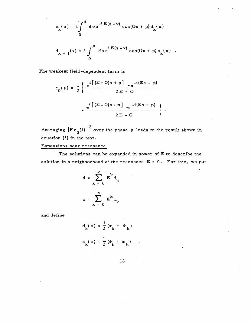
S - i E ( s -x) c ( s ) = i/ d x e cos(Gx t p)d k ( x ) k
S i E ( s -x ) ( s ) = i J d x e
0
cos(Gx t p ) c k ( x ) . dk t 1
The weakest field-dependent te rm i s
i [ ( E + G ) s + p ] -i(Es - p) - e
2 2 E t G c o b ) = q e
i [ (E - G)s - p ] -e - i (Es t p)
2E - G 1
2 Averaging ] F c o ( l ) 1 equation (3) in the text.
Expansions near resonance
over the phase p leads to the resul t shown in
The solutions can be expanded in power of E to describe the
solution in a neighborhood at the resonance E = 0. F o r this, we put
d = Ekdk k = O
k c = c E C k
k = 0
and define
1 c ( 8 ) = - ($ - 4 k ) . k 2 k
18

These new functions satisfy the system
# k - i F cos(Gs t p) k i a k - l
4 k t i F cos(Gs i p ) @ k = i + k - l .
For k = 0, the initial data a re satisfied by the solutions
F G i - [sin(Gs t p) - s i n p ]
= e
. F -1- G [s in(& t p) - s i n p ]
4 ( s ) = e 0
The higher order functions could be obtained, with some pain, f r o m
the recursions k 2 1
F G i - sin(Gs t p)
#,(s) = i e
F C -i - sin(Gs t p)
6 ( s ) = i e k S F
C i - sin(Gx t p) dx ‘k - 1 ( x ) e
0
k - Note that 4 ( s ) = ( - ) # , ( s ) . k
19

Restricting ourselves to the resonance solution,
= cos [ G (sin(Gs t p) - sinp) ]
E = 0
F d 0
F 0 G
c = s in[ - (sin(Gs t p) - sinp) ] .
To this approximation
2 * = sin [ F (sin(G t p) - s i n p ) ]
where
b
D - - * F
= E - w F
To average this resul t over the phase p , we note that we can write
I C 2 a ( - 1 1 = F { l - c o s [ 2 F 1 * s i n p ( c o s G - l ) ] c o s [ 2 F * c o s p s i n G ] q v * *
t s i n [ 2 F sinp(cos G - l ) ] s i n [ 2 F c o s p s i n G ] } .
The third t e rm in the bracket can be dropped, since i t is anti-
symmetric about p = 0 . Using the expansions
cos (x sin p)
cos ( x cos p) k = O ] = 2 Ck J Z k ( x ) c o s 2k
where € = 1, € = 2 (k 2 l ) , and noting that 0 k u
20

we have, averaging over p.
rlr rlr ?-
where A = 2 F (cos G - l), B = 2F1' s in G . By Graf's Addition
Theorem
= J o ( m ) .
Thus,
.lr 2 R 1 * <Cq ( T ) > ~ = ~ ( 1 t J0(2F (cos G - 1 ) ) Jo(2FTsinG)
* G 2 -2 J0(4F sin - ) }
which leads to equation (4).
F o r a particle with no Doppler shift, W = 0: D
2 b R ) 1 1 2 = - (1 - Jo(
Iw = 0 D
as given in equation (5) . L
9 To derive even the linear dependence of I C I on E appears to
be a very difficult problem. Solutions for large F (saturating fields)
can be obtained.
could be determined to linear te rms , i t s form for large F could be
matched to the la rge-F solutions to give a uniform solution for
saturating fields.
These a r e singular at E = 0, but i f the E- se r i e s
The solutions for large F wi l l not be discussed in this report.
21

Appendix B
The problem is to solve the t ime -dependent SchrGdinger
e quation
i R !!k = (Ho t V) #I a t
where
using the Rayleigh-SchrGdinger Perturbation Method [7 1 - The initial
conditions a r e more general than in Section 2, i.e., we assume the
values
and look for the solutions at t = T . The perturbation is :
i w t - iwt V = % b e V = * b e
PQ v 9 p
The general solution has been given by Ramsey [2]as follows ; we just
introduce the abbreviations
0 = # / a W = Uq/R P P 9
and assume these values to be constant throughout the interaction space.
(This simplifies somewhat the computations and i t is valid €or this case
since we can assume the Zeemann and Stark Shifts to be negligible. )
The solutions a r e :
22

a T t cos-IC a T (t ) c (t t T) = { [ i cos e sin- P 1 2 2 P 1
a T iwtl t [ i s in e sin - e 3 Cq(tl) ] 2
i T / 2 ( w - w -us) P X e
a T - iwt l c (t + ~ ) = ( [ i s i n ~ s i n - e 2 . ]cp(tl) 9 1
a T a T t cos-]IC (t ) }
2 9 1 t [ - i cos B sin- 2
m I -i-(ut % t w ) 2 9 X e
where s i n e , cos 8 , a , a r e the same as defined in Section 3A. The
computation for three successive separated oscillating fields follows
closely that of Ramsey [ 2 , pp. 127- 1281; we used the same notation in
order to allow an easy comparison. Before Proceeding fur ther , le t us
note the special case of b = 0 , which is used for the regions between
the oscillating fields : -wpT
0 C (t t T) = . C (t )e P 1 P 1
T - i w 9 Oc (t t T) = c (t )e
9 1 9 1
To avoid further complication, we res t r ic t ourselves to the case of
equal b in all three field regions of length
length L , where b = 0 ( s z e f ig . 4).
, separated by regions of
The molecule enters the first region at t = 0 and leaves i t at 1 T = 7. During that time 7, b is constant (not exactly true, but s impler) .
Fur thermore , C ( 0 ) = 1, C ( 0 ) = 0 . We then have, after the f i r s t P 9
23

field region:
a T a T 2 t cos - ) C ( r ) = ( i c o s e s i n - P 2
7 X e i- 2 (-P - WS)
-i- 7 ( a t o -t )
C q ( r ) = ( i s in8 s in - ) a r X e 2 P 9 2
These resul ts a r e the initial conditions for the next s tep : b = 0 for
time T . We obtain
c ( r t T) = ( i c o s e sin t cos - ) a r P 2 2
+ i[' ( w - w - wq) - w p ~ ] 2 P X e
a r C (7 t T) = ( isinG sin -) 9 2
T - i [ z ( w + w P + w ) 9 + wqT] .
X e
In the second Eield region, another perturbation b is applied for time
7 , with the above C (7 t T) , C (7 t T) as initial conditions. We
therefore apply the general solutions by setting therein: t l = T + T
and T = and obtain:
P 9
C ( 2 T t T) = { [ i s i n g s i n z t cos C (7 t T ) P 2 2 P
T + i - ( w - w - 0 1 2 P 9 X e
24
,

IC ( 7 + T ) a7 -io (7 t T)
C (27 t T) = [ [ i sin 8 sin - e q 2 P
a7 t - i cos 8 sin 5 t cos - 1 c (7 t T) 3
2 2 q
Up to this point, the results a r e copied out of reference [ 2 ] . To go
beyond, we apply again b = 0 for t ime T and obtain:
- i w T C (27 t 2T)= C (27 t T) e P
C (27 t 2T)= C (27 t T) e 9
P P - i w T
9 9
Finally we need only:
C (37 t 2T) = [ [ i s ine sin a7 e -iw(27 ' 2T] C (2, . + 2T) q 2 P
t [ - i c o s e sin- a7 t cos ] C (27 t 2T) ] 2 2 9
-'(wtw + w ) .P 9 2
X e
in order to obtain:
2 = ( 1 C (37t 2T) I ) 9 P¶ q
3P
where the ( )just denote that this is an expectation value.
need for a further averaging over.initia1 phases of entry into the f i r s t
field, since Ramsey's solution is independent of the initial phase.
is no longer t rue for the case treated in Appendix A. )
There is no
(This
For the detailed computation we introduce the following
substitutions:

a7 a = i sin 8 sin - 2
a r @ = i cos 8 sin - 2
a7 y = cos - 2 .
Then:
7 i[- ( 0 - w - w ) - w T I G ( 2 7 t T ) = [ ( p t Y ) 2 e 2 P 9 P
P
- i r L ( w t w t u ) t w T - u ( T t T ) ] ] 2 2 P 9 9
+ C Y e
i L ( w - w - w ) 2 P ' 9 X e
7 i[- ( w - up - wq) - w T - w ( 7 t T ) ] 2 P
-i[z ( w t w t o ) t w T I ]
C . (27 t T ) = {a ( p t Y ) e 9
7
P 9 9 +- ( Y - 8 ) ae
We want to obtain
2 T ) ' C ( 2 7 + 2 T ) C. ( 3 7 + 2 T ) = frwe 9 P
This expression can be writ ten in the following form:
26

i 5 , i 5, i 5, i t4 C (37 + 2 T ) = Ale t AZe t A3 e t A4e
9
where
3 A2 = CY
3
And by introducing X = w
we have
- w - 0, w - w = u0 :. X = w0 - w q P q P
5 , = 1
- - ( 2 T t 3 7 ) ( ~ t W t W ) t h T 2 P 9
1 - - - - (2T + 3 7 ) ( W t w w ) - A T 54 2 P 9
and thus:
i A T - i X T - i p t A t A 3 t A e ) e . . 2 4 C (37 t 2 T ) = (Ale
q
Of this las t expression we need only the t e rms in the - i p
parenthesis, since the factor e drops out in calculating the
modulus of this complex quantity, and we obtain, by using
) - i h T
+ e 1 i h T 2i 1 i A T t e - i X T 2
s in X T = - (e
c o s h T = - (e 1

the final solution:
2 = 4 sin 8 sin2 aT { cos 8 s in a7 sinX T 2
3P P, 9
having re-substituted for CY, 5, and Y .
28