notes on primality testing and public key cryptography ...jean/rsa-primality-testing.pdf · several...
TRANSCRIPT

Notes on Primality TestingAnd Public Key CryptographyPart 1: Randomized Algorithms
Miller–Rabin and Solovay–Strassen Tests
Jean Gallier and Jocelyn QuaintanceDepartment of Computer and Information Science
University of PennsylvaniaPhiladelphia, PA 19104, USAe-mail: [email protected]
c© Jean Gallier
February 27, 2019
Contents
Contents 2
1 Introduction 51.1 Prime Numbers and Composite Numbers . . . . . . . . . . . . . . . . . . . . 51.2 Methods for Primality Testing . . . . . . . . . . . . . . . . . . . . . . . . . . 61.3 Some Tests for Compositeness . . . . . . . . . . . . . . . . . . . . . . . . . . 9
2 Public Key Cryptography 132.1 Public Key Cryptography; The RSA System . . . . . . . . . . . . . . . . . . 132.2 Correctness of The RSA System . . . . . . . . . . . . . . . . . . . . . . . . . 182.3 Algorithms for Computing Powers and Inverses Modulo m . . . . . . . . . . 222.4 Finding Large Primes; Signatures; Safety of RSA . . . . . . . . . . . . . . . 26
3 Primality Testing Using Randomized Algorithms 33
4 Basic Facts About Groups, and Number Theory 374.1 Groups, Subgroups, Cosets . . . . . . . . . . . . . . . . . . . . . . . . . . . . 374.2 Cyclic Groups . . . . . . . . . . . . . . . . . . . . . . . . . . . . . . . . . . . 504.3 Rings and Fields . . . . . . . . . . . . . . . . . . . . . . . . . . . . . . . . . 604.4 Primitive Roots . . . . . . . . . . . . . . . . . . . . . . . . . . . . . . . . . . 674.5 Which Groups (Z/nZ)∗ Have Primitive Roots . . . . . . . . . . . . . . . . . 754.6 The Lucas Theorem, PRIMES is in NP . . . . . . . . . . . . . . . . . . . . 804.7 The Structure of Finite Fields . . . . . . . . . . . . . . . . . . . . . . . . . . 90
5 The Miller–Rabin Test 935.1 Square Roots of Unity . . . . . . . . . . . . . . . . . . . . . . . . . . . . . . 945.2 The Fermat Test; F -Witnesses and F -Liars . . . . . . . . . . . . . . . . . . . 965.3 Carmichael Numbers . . . . . . . . . . . . . . . . . . . . . . . . . . . . . . . 995.4 The Miller–Rabin Test; MR-Witnesses and MR-Liars . . . . . . . . . . . . . 1035.5 The Monier–Rabin Bound on the Size of the Set of MR-Liars . . . . . . . . . 1165.6 The Least MR-Witness for n . . . . . . . . . . . . . . . . . . . . . . . . . . . 121
6 The Solovay–Strassen Test 1256.1 Quadratic Residues . . . . . . . . . . . . . . . . . . . . . . . . . . . . . . . . 125
2
CONTENTS 3
6.2 The Legendre Symbol . . . . . . . . . . . . . . . . . . . . . . . . . . . . . . . 1276.3 The Jacobi Symbol . . . . . . . . . . . . . . . . . . . . . . . . . . . . . . . . 1346.4 The Solovay–Strassen Test; E-Witnesses and E-Liars . . . . . . . . . . . . . 1376.5 The Quadratic Reciprocity Law . . . . . . . . . . . . . . . . . . . . . . . . . 1406.6 A Randomized Algorithm to Find a Square Root mod p . . . . . . . . . . . 1446.7 Proof of the Quadratic Reciprocity Law . . . . . . . . . . . . . . . . . . . . . 1506.8 Eisenstein’s Proof of the Quadratic Reciprocity Law . . . . . . . . . . . . . . 1556.9 Strong Pseudoprimes are Euler Pseudoprimes . . . . . . . . . . . . . . . . . 158
Bibliography 163
4 CONTENTS

Chapter 1
Introduction
1.1 Prime Numbers and Composite Numbers
Prime numbers have fascinated mathematicians and more generally curious minds for thou-sands of years. What is a prime number? Well, 2, 3, 5, 7, 11, 13, . . . , 9973 are prime numbers.The defining property of a prime number p is that it is a positive integer p ≥ 2 that is onlydivisible by 1 and p. Equivalently, p is prime if and only if p is a positive integer p ≥ 2 thatis not divisible by any integer m such that 2 ≤ m < p. A positive integer n ≥ 2 which isnot prime is called composite. Observe that the number 1 is considered neither a prime nora composite. For example, 6 = 2 · 3 is composite. Is 3 215 031 751 composite? Yes, because
3 215 031 751 = 151 · 751 · 28351.
The above number has the remarkable property of being the only composite integer less than25 · 109 which a strong pseudoprime simultaneously to the bases 2, 3, 5, 7; see Definition 5.5,and Ribenboim [18] (Chapter 2, Section XI).
Even though the definition of primality is very simple, the structure of the set of primenumbers is highly nontrivial. The prime numbers are the basic building blocks of the natu-ral numbers because of the following theorem bearing the impressive name of fundamentaltheorem of arithmetic.
Theorem 1.1. Every natural number n ≥ 2 has a unique factorization
n = pi11 pi22 · · · p
ikk ,
where the exponents i1, . . . , ik are positive integers and p1 < p2 < · · · < pk are primes.
Every book on number theory has a proof of Theorem 1.1. The proof is not difficult anduses induction. It has two parts. The first part shows the existence of a factorization. Thesecond part shows its uniqueness. For example, see Apostol [1] (Chapter 1, Theorem 1.10).
How many prime numbers are there? Many! In fact, infinitely many.
5

6 CHAPTER 1. INTRODUCTION
Theorem 1.2. The set of prime numbers is infinite.
Proof. We give three proofs. These proofs only use the fact that every integer greater than1 has some prime divisor.
(1) (Euclid) Suppose that p1 = 2 < p2 = 3 < · · · < pm are all the primes. ConsiderN = p1p2 · · · pm + 1. The number N must be divisible by some prime p (p = Nis possible). Then p must be one of the pi, so p = pi divides N − p1p2 · · · pm = 1,contradicting the fact that pi ≥ 2.
(2) (Kummer) Suppose that p1 = 2 < p2 = 3 < · · · < pm are all the primes, as in (1),but this time let N = p1p2 · · · pm. Observe that N > 2. The number N − 1 must bedivisible by one of the primes pi (pi = N − 1 is possible). But if pi divides N − 1, thenpi divides N − (N − 1) = 1, a contradiction.
(3) (Hermite) We prove that for every natural number n ≥ 2, there is some prime p > n.Consider N = n! + 1. The number N must be divisible by some prime p (p = N ispossible). Any prime p dividing N is distinct from 2, 3, . . . , n, since otherwise p woulddivide N − n! = 1, a contradiction.
There are many more proofs; see Ribenboim [18].
The problem of determining whether a given integer is prime is one of the better knownand most easily understood problems of pure mathematics. This problem has caught theinterest of mathematicians again and again for centuries. However, it was not until the 20thcentury that questions about primality testing and factoring were recognized as problemsof practical importance, and a central part of applied mathematics. The advent of cryp-tographic systems that use large primes, such as RSA, was the main driving force for thedevelopment of fast and reliable methods for primality testing. Indeed, as we see in Chapter2, in order to create RSA keys, one needs to produce large prime numbers. How do we dothat?
1.2 Methods for Primality Testing
The general strategy to test whether an integer n > 2 is prime or composite is to choosesome property, say A, implied by primality, and to search for a counterexample a to thisproperty for the number n, namely some a for which property A fails. We look for propertiesfor which checking that a candidate a is indeed a countexample can be done quickly.
Typically, together with the number n being tested for primality, some candidate coun-terexample a is supplied to an algorithm which runs a test to determine whether a is really acounterexample to property A for n. If the test says that a is a counterexample, also calleda witness , then we know for sure that n is composite. If the algorithm reports that a is not awitness to the fact that n is composite, does this imply that n is prime? Unfortunately, no.

1.2. METHODS FOR PRIMALITY TESTING 7
This is because, there may be some composite number n and some candidate counterexamplea for which the test says that a is not a countexample. Such a number a is called a liar .The other reason is that we haven’t tested all the candidate counterexamples a for n.
The remedy is to make sure that we pick a property A such that if n is composite, then atleast some candidate a is not a liar, and to test all potential countexamples a. The difficultyis that trying all candidate countexamples can be too expensive to be practical.
The following analogy may be helpful to understand the nature of such a method. Sup-pose we have a population and we are interested in determining whether some individualis rich or not (we will say that someone who is not rich is poor). Every individual n hasseveral bank accounts a, and there is a test to check whether a bank account a has a negativebalance. The test has the property that if it is applied to an individual n and to one of itsbank accounts a, and if it is positive (it says that account a has a negative balance), thenthe individual n is definitely poor. Note that we are assuming that a rich person is honest,namely that all bank accounts of a rich person have a nonnegative balance. This may bean unrealistic assumption. But if the test is negative (which means that account a has anonnegative balance), this does not imply that n is rich.
The problem is that the test may not be 100% reliable. It is possible that an individualn is poor, yet the test is negative for account a (account a has a nonnegative balance). Wemay also not have tested all the accounts of n.
One way to deal with this problem is to use probabilities. If we know that the conditionalprobability that the test is positive for some account a given that n is poor is greater thanp ≥ 1/2, then we can apply the test to ` accounts chosen independently at random. It iseasy to show that the conditional probability that the test is negative ` times given that anindividual n is poor is less than (1−p)`. For p close to 1 and ` large enough, this probabilityis very small. Thus, if we have high confidence in the test (p is close to 1) and if an individualn is poor, it is very unlikely that the test will be negative ` times.
Actually, what we would really like to know is the conditional probability that the indi-vidual n is rich given that the test is negative ` times. If the probability that an individualn is rich is known, then the above conditional probability can be computed using Bayes’srule. We will show how to do this later. A Monte Carlo algorithm does not give a definiteanswer. However, if ` is large enough (say ` = 100), then the conditional probability thatthe property of interest holds (here, n is rich), given that the test is negative ` times, is veryclose to 1. In other words, if ` is large enough and if the test is negative ` times, then wehave high confidence that n is rich.
There are two classes of primality testing algorithms:
(1) Algorithms that try all possible countexamples, and for which the test does not lie.These algorithms give a definite answer: n is prime or n is composite. Until 2002,no algorithms running in polynomial time, were known. The situation changed in2002 when a paper with the title “PRIMES is in P,” by Agrawal, Kayal and Saxena,

8 CHAPTER 1. INTRODUCTION
appeared on the website of the Indian Institute of Technology at Kanpur, India. Inthis paper, it was shown that testing for primality has a deterministic (nonrandomized)algorithm that runs in polynomial time.
We will not discuss algorithms of this type here, and instead refer the reader to Crandalland Pomerance [3] and Ribenboim [18].
(2) Randomized algorithms. To avoid having problems with infinite events, we assumethat we are testing numbers in some large finite interval I. Given any positive integerm ∈ I, some candidate witness a is chosen at random. We have a test which, given mand a potential witness a, determines whether or not a is indeed a witness to the factthat m is composite. Such an algorithm is a Monte Carlo algorithm, which means thefollowing:
(1) If the test is positive, then m ∈ I is composite. In terms of probabilities, thisis expressed by saying that the conditional probability that m ∈ I is compositegiven that the test is positive is equal to 1. If we denote the event that somepositive integer m ∈ I is composite by C, then we can express the above as
Pr(C | test is positive) = 1.
(2) If m ∈ I is composite, then the test is positive for at least 50% of the choices fora. We can express the above as
Pr(test is positive | C) ≥ 1
2.
This gives us a degree of confidence in the test.
The contrapositive of (1) says that if m ∈ I is prime, then the test is negative. If wedenote by P the event that some positive integer m ∈ I is prime, then this is expressedas
Pr(test is negative | P ) = 1.
If we repeat the test ` times by picking independent potential witnesses, then the con-ditional probability that the test is negative ` times given that n is composite, writtenPr(test is negative ` times | C), is given by
Pr(test is negative ` times | C) = Pr(test is negative | C)`
= (1− Pr(test is positive | C))`
≤(
1− 1
2
)`=
(1
2
)`,
1.3. SOME TESTS FOR COMPOSITENESS 9
where we used Property (2) of a Monte Carlo algorithm that
Pr(test is positive | C) ≥ 1
2
and the independence of the trials. This confirms that if we run the algorithm ` times, thenPr(test is negative ` times | C) is very small. In other words, it is very unlikely that the testwill lie ` times (is negative) given that the number m ∈ I is composite.
If the probabilty Pr(P ) of the event P is known, which requires knowledge of the distri-bution of the primes in the interval I, then the conditional probability
Pr(P | test is negative ` times)
can be determined using Bayes’s rule. We do this in Section 5.4.
Our Monte Carlo algorithm does not give a definite answer. However, if ` is large enough(say ` = 100), then the conditional probability that the number n being tested is prime giventhat the test is negative ` times, is very close to 1.
1.3 Some Tests for Compositeness
The algorithms that we will discuss test three kinds of properties:
(1) The Fermat test . For any odd integer n ≥ 5, pick randomly some a ∈ 2, . . . , n− 2,and test whether
an−1 6≡ 1 (mod n).
If the test is positive, then return n is composite, else n is a “probable prime.”
(2) The Miller–Rabin test . For any odd integer n ≥ 5, write n − 1 = 2kt with t odd andk ≥ 1, pick randomly some a ∈ 2, . . . , n− 2, and test whether
(a) at 6≡ ±1 (mod n), and
(b) a2it 6≡ n− 1 (mod n), for all i with 1 ≤ i ≤ k − 1.
If the test is positive, then return n is composite, else n is a “probable prime.”
(3) The Euler test . For any odd integer n ≥ 5, pick randomly some a ∈ 2, . . . , n − 2,and test whether (
a
n
)a(n−1)/2 6≡ 1 (mod n).
If the test is positive, then return n is composite, else n is a “probable prime.” Theexpression
(an
)is the Jacobi symbol . It is a generalization of the Legendre symbol .
These symbols have to do with quadratic residues. Given any integer n ≥ 2, an integer
10 CHAPTER 1. INTRODUCTION
m such that gcd(m,n) = 1 is said to be a quadratic residue mod n (or a square mod n)if the congruence
x2 ≡ m (mod n)
has a solution. Let p be an odd prime. For any integer m, the Legendre symbol(mp
)is
defined as follows:
(m
p
)=
+1 if m is a quadratic residue modulo p
−1 if m is a quadratic nonresidue modulo p
0 if p divides m.
The Jacobi symbol(mP
)is defined for a positive odd integer P ≥ 3 in terms of the
prime factorization of P ; see Definition 6.3.
The remarkable fact about the Legendre symbol is that it gives us an efficient methodfor testing whether a number m is a quadratic residue mod n without actually solving thecongruence x2 ≡ m (mod n). The Jacobi symbol gives us an even more efficient methodwhich avoids factoring. The reason is that there is an unexpected and deep relationshipbetween the symbols
(pq
)and
(qp
), known as the law of quadratic reciprocity .
The law of quadratic reciprocity was conjectured by Legendre and proved by Gauss, whogave no less than seven proofs. It is one of the gems of number theory, and we will prove itin Section 6.7.
Property (1) of a Monte Carlo algorithm holds for all three tests. Next we need to showthat Property (2) holds. For this, it is helpful to define the following sets of liars: for everyodd composite n ≥ 3, write n− 1 = 2kt with t odd and k ≥ 1,
LFn = a ∈ 1 ≤ a ≤ n− 1 | an−1 ≡ 1 (mod n),LMRn = a ∈ 1, . . . , n− 1, either at ≡ 1 (mod n),
or a2it ≡ n− 1 (mod n), for some i with 0 ≤ i ≤ k − 1
LEn = a ∈ 1, . . . , n |(a
n
)a(n−1)/2 ≡ 1 (mod n).
The set LFn is called the set of F -liars (Fermat liars), the set LMRn is called the set of
MR-liars (Miller–Rabin liars) and the set LEn is called the set of E-liars (Euler liars).
It is easy to see that all three sets of liars are subsets of the multiplicative group (Z/nZ)∗
of invertible elements of the ring Z/nZ. The order of this group is ϕ(n), a famous functiondue Euler, where ϕ(n) is the number of integers a with 1 ≤ a ≤ n such that gcd(a, n) = 1.Obviously, ϕ(n) < n if n > 1.
Now if we could prove that our sets of liars are proper subsets of (Z/nZ)∗ of size at mostϕ(n)/2, then we woud be done, because the conditional probability that a is a liar given thatn is composite would be at most ϕ(n)/(2n) < 1/2.
1.3. SOME TESTS FOR COMPOSITENESS 11
It turns out that both LFn and LEn are subgroups of (Z/nZ)∗, but unfortunately LMRn is
not closed under multiplication. If we can prove that LFn and LEn are proper subgroups of(Z/nZ)∗, then by Lagrange’s theorem we are done, because the order of a subgroup dividesthe order of the group, so a proper subgroup has order at most ϕ(n)/2.
Solovay and Strassen proved that LEn is a proper subgroup of (Z/nZ)∗; see Theorem 6.12.This is a nice an nontrivial proof.
As to LFn , unfortunately there are composites n for which LFn = (Z/nZ)∗; all numbersa ∈ 1. . . . , n − 1 are liars! Such trouble makers are called Carmichael numbers . Thesmallest one is 561 = 3 × 11 × 17. More bad news: there are infinitely many Carmichaelnumbers; see Section 5.3.
The Miller–Rabin test, which is a stronger version of the Fermat test, is immune toCarmichael numbers. Indeed, even though LMR
n is not a group, it is contained is a subgroupS(n) of (Z/nZ)∗ of the form
S(n) = a ∈ (Z/nZ)∗ | am ≡ ±1 (mod n),
for some suitable m (depending on n), such that m divides n− 1. Monier and Rabin provedthat the subgroup S(n) is a proper subgroup of (Z/nZ)∗, and that if n > 9, then the orderof S(n) is at most ϕ(n)/4 ≤ (n − 1/4); see Theorem 5.13. This is a beautiful proof thatmixes combinatorial and number theoretic ideas. We also show that LMR
n ⊆ LEn ; see Section6.9.
Having some powerful methods for testing for primality, we show in Chapter 2 howprime numbers can be used for public key cryptography, and in particular we present theRSA system.
The investigation of primality testing algorithms and cryptographic methods provideswonderful and strong motivations for delving more deeply into number theory.
One will quickly realize that in order to get more than a superficial understanding ofrandomized algorithms for primality testing, one needs to know some basic properties ofgroups, rings, and fields, and in particular properties of cyclic groups. In particular, themultiplicative group (Z/nZ)∗ of invertible elements of the ring Z/nZ plays an importantrole. It is crucial to know when the group (Z/nZ)∗ is cyclic, which means that it is generatedby a single element called a primitive root . A famous theorem of Gauss tells us that thegroup (Z/nZ)∗ has a primitive root iff n = 2, 4, pm, or 2pm where p is an odd prime. Wegive a complete proof of this result in Sections 4.4 and 4.5. In Sections 4.1, 4.2, and 4.3, weprovide a review of groups, rings, and fields.
Quadratic residues, the Legendre symbol, and the Jacobi symbol, play a crucial role inthe Solovay–Strassen test. We also present a randomized algorithm for finding the squareroot of a number which is a quadratic residue modulo an odd prime. One of the jewels ofnumber theory is the law of quadratic reciprocity , which was also proved by Gauss (in fact,

12 CHAPTER 1. INTRODUCTION
he gave seven proofs). The law of quadratic reciprocity relates the symbols(pq
)and
(qp
),
and yields a fast method to evaluate the Legendre (and the Jacobi) symbol.
Even though it is not absolutely necessary to know how to prove the law of quadraticreciprocity to understand the Solovay–Strassen test, we feel that it would be a shame not toinclude a proof, so we do. In fact, we give two proofs. The second one, due to Eisenstein(1845), is particularly original because is uses a trigonometric identity.
Our philosophy is that primality testing and cryptographic methods give us a great excuseto present some deep and beautiful mathematics, with an emphasis on number theory. Wealso believe that it is important to prove everything we state, and we (mostly) do!
Two excellent references on cryptography and its mathematical underpinnings are Hoff-stein, Pipher and Silverman [8], and Shoup [21]. A more advanced treatment is given inCrandall and Pomerance’s remarkable book [3] and in Ribenboim’s delightful book [18];Dietzfelbinger [4] is also very good but less encyclopedic. An easy going and delightful intro-duction to number theory is found in Silverman [22]. More advanced presentations are givenin Apostol [1], Niven, Zuckerman, and Montgomery [16], and Ireland and Rosen [9]. Serre’sbook [20] is another great source for those intetested in advanced topics in number theory.For those interested in original sources, Dirichlet–Dedekind [12] is a real jewel. This book isbased on a manuscript of Dirichlet but was actually written by Richard Dedekind and pub-lished in 1863 after Dirichlet’s death in 1859. The English translation is by John Stillwell.The reader will be pleasantly surprised to see how clear and lively the style is, and will find amasterly exposition of many of the results from Gauss’s famous Disquisitiones Arithmeticae[7]. Incidently, if you can get your hands on a translation of Gauss’s masterpiece, you willexperience what it is to be exposed to pure genius.
Sorry, we will not discuss applications of elliptic curves and lattice methods to primalitytesting, factoring, and cryptographic methods, in these notes. Perhaps in another set ofnotes ...
Chapter 2
Public Key Cryptography
2.1 Public Key Cryptography; The RSA System
Ever since written communication was used, people have been interested in trying to concealthe content of their messages from their adversaries. This has led to the development oftechniques of secret communication, a science known as cryptography .
The basic situation is that one party, A, say Albert, wants to send a message to anotherparty, J, say Julia. However, there is a danger that some ill-intentioned third party, Machi-avelli, may intercept the message and learn things that he is not supposed to know aboutand as a result, do evil things. The original message, understandable to all parties, is knownas the plain text . To protect the content of the message, Albert encrypts his message. WhenJulia receives the encrypted message, she must decrypt it in order to be able to read it. BothAlbert and Julia share some information that Machiavelli does not have, a key . Without akey, Machiavelli, is incapable of decrypting the message and thus, to do harm.
There are many schemes for generating keys to encrypt and decrypt messages. We are go-ing to describe a method involving public and private keys known as the RSA Cryptosystem,named after its inventors, Ronald Rivest, Adi Shamir, and Leonard Adleman (1978), basedon ideas by Diffie and Hellman (1976). We highly recommend reading the orginal paperby Rivest, Shamir, and Adleman [19]. It is beautifully written and easy to follow. A veryclear, but concise exposition can also be found in Koblitz [10]. An encyclopedic coverage ofcryptography can be found in Menezes, van Oorschot, and Vanstone’s Handbook [14].
The RSA system is widely used in practice, for example in SSL (Secure Socket Layer),which in turn is used in https (secure http). Any time you visit a “secure site” on theInternet (to read e-mail or to order merchandise), your computer generates a public key anda private key for you and uses them to make sure that your credit card number and otherpersonal data remain secret. Interestingly, although one might think that the mathematicsbehind such a scheme is very advanced and complicated, this is not so. Therefore, in thissection, we are going to explain the basics of RSA.
The first step is to convert the plain text of characters into an integer. This can be done
13

14 CHAPTER 2. PUBLIC KEY CRYPTOGRAPHY
easily by assigning distinct integers to the distinct characters, for example, by convertingeach character to its ASCII code. From now on, we assume that this conversion has beenperformed.
The next and more subtle step is to use modular arithmetic. We assume that the readerhas some familiarity with basic facts of arithmetic (greatest common divisors, etc.). A“gentle” exposition is given in Gallier [6], Chapter 5. We pick a (large) positive integer mand perform arithmetic modulo m. Let us explain this step in more detail.
Recall that for all a, b ∈ Z, we write a ≡ b (mod m) iff a − b = km, for some k ∈ Z,and we say that a and b are congruent modulo m. We already know that congruence is anequivalence relation but it also satisfies the following properties.
Proposition 2.1. For any positive integer m, for all a1, a2, b1, b2 ∈ Z, the following proper-ties hold. If a1 ≡ b1 (modm) and a2 ≡ b2 (modm), then
(1) a1 + a2 ≡ b1 + b2 (modm).
(2) a1 − a2 ≡ b1 − b2 (modm).
(3) a1a2 ≡ b1b2 (modm).
Proof. We only check (3), leaving (1) and (2) as easy exercises. Because a1 ≡ b1 (mod m)and a2 ≡ b2 (modm), we have a1 = b1 + k1m and a2 = b2 + k2m, for some k1, k2 ∈ Z, and so
a1a2 = (b1 + k1m)(b2 + k2m) = b1b2 + (b1k2 + k1b2 + k1mk2)m,
which means that a1a2 ≡ b1b2 (modm). A more elegant proof consists in observing that
a1a2 − b1b2 = a1(a2 − b2) + (a1 − b1)b2= (a1k2 + k1b2)m,
as claimed.
Proposition 2.1 allows us to define addition, subtraction, and multiplication on equiva-lence classes modulo m.
Definition 2.1. Given any positive integer m, we denote by Z/mZ the set of equivalenceclasses modulo m. If we write a for the equivalence class of a ∈ Z, then we define addition,subtraction, and multiplication on residue classes as follows:
a+ b = a+ b
a− b = a− bab = ab.
2.1. PUBLIC KEY CRYPTOGRAPHY; THE RSA SYSTEM 15
The above operations make sense because a+ b does not depend on the representativeschosen in the equivalence classes a and b, and similarly for a− b and ab. Each equivalenceclass a contains a unique representative from the set of remainders 0, 1, . . . ,m−1, modulom, so the above operations are completely determined by m×m tables. Using the arithmeticoperations of Z/mZ is called modular arithmetic.
For an arbitrary m, the set Z/mZ is an algebraic structure known as a ring . Additionand subtraction behave as in Z but multiplication is stranger. For example, when m = 6,
2 · 3 = 0
3 · 4 = 0,
inasmuch as 2 · 3 = 6 ≡ 0 (mod 6), and 3 · 4 = 12 ≡ 0 (mod 6). Therefore, it is not truethat every nonzero element has a multiplicative inverse. However, it is known (see Gallier[6], Chapter 5) that a nonzero integer a has a multiplicative inverse iff gcd(a,m) = 1 (usethe Bezout identity). For example,
5 · 5 = 1,
because 5 · 5 = 25 ≡ 1 (mod 6).
As a consequence, when m is a prime number, every nonzero element not divisible by mhas a multiplicative inverse. In this case, Z/mZ is more like Q; it is a finite field . However,note that in Z/mZ we have
1 + 1 + · · ·+ 1︸ ︷︷ ︸m times
= 0
(because m ≡ 0 (modm)), a phenomenom that does not happen in Q (or R).
The RSA method uses modular arithmetic. One of the main ingredients of public keycryptography is that one should use an encryption function, f : Z/mZ → Z/mZ, which iseasy to compute (i.e., can be computed efficiently) but such that its inverse f−1 is practicallyimpossible to compute unless one has special additional information. Such functions areusually referred to as trapdoor one-way functions . Remarkably, exponentiation modulo m,that is, the function, x 7→ xe mod m, is a trapdoor one-way function for suitably chosen mand e.
Thus, we claim the following.
(1) Computing xe modm can be done efficiently .
(2) Finding x such that
xe ≡ y (modm)
with 0 ≤ x, y ≤ m−1, is hard, unless one has extra information about m. The functionthat finds an eth root modulo m is sometimes called a discrete logarithm.

16 CHAPTER 2. PUBLIC KEY CRYPTOGRAPHY
We explain shortly how to compute xe mod m efficiently using the square and multiplymethod also known as repeated squaring .
As to the second claim, actually, no proof has been given yet that this function is aone-way function but, so far, this has not been refuted either.
Now, what’s the trick to make it a trapdoor function?
What we do is to pick two distinct large prime numbers, p and q (say over 200 decimaldigits), which are “sufficiently random” and we let
m = pq.
Next, we pick a random e, with 1 < e < (p− 1)(q − 1), relatively prime to(p− 1)(q − 1).
Because gcd(e, (p− 1)(q− 1)) = 1, there is some d with 1 < d < (p− 1)(q− 1), such thated ≡ 1 (mod (p− 1)(q − 1)).
Then, we claim that to find x such that
xe ≡ y (modm),
we simply compute yd modm, and this can be done easily, as we claimed earlier. The reasonwhy the above “works” is that
xed ≡ x (modm), (∗)
for all x ∈ Z, which we prove later.
Setting up RSA
In summary to set up RSA for Albert (A) to receive encrypted messages, perform the fol-lowing steps.
1. Albert generates two distinct large and sufficiently random primes, pA and qA. Theyare kept secret.
2. Albert computes mA = pAqA. This number called the modulus will be made public.
3. Albert picks at random some eA, with 1 < eA < (pA − 1)(qA − 1), so thatgcd(eA, (pA − 1)(qA − 1)) = 1. The number eA is called the encryption key and it willalso be public.
4. Albert computes the inverse, dA = e−1A modulo (pA− 1)(qA− 1), of eA. This number iskept secret. The pair (dA,mA) is Albert’s private key and dA is called the decryptionkey .
5. Albert publishes the pair (eA,mA) as his public key .

2.1. PUBLIC KEY CRYPTOGRAPHY; THE RSA SYSTEM 17
Encrypting a Message
Now, if Julia wants to send a message, x, to Albert, she proceeds as follows. First, she splitsx into chunks, x1, . . . , xk, each of length at most mA − 1, if necessary (again, I assume thatx has been converted to an integer in a preliminary step). Then she looks up Albert’s publickey (eA,mA) and she computes
yi = EA(xi) = xeAi modmA,
for i = 1, . . . , k. Finally, she sends the sequence y1, . . . , yk to Albert. This encrypted messageis known as the cyphertext . The function EA is Albert’s encryption function.
Decrypting a Message
In order to decrypt the message y1, . . . , yk that Julia sent him, Albert uses his private key(dA,mA) to compute each
xi = DA(yi) = ydAi modmA,
and this yields the sequence x1, . . . , xk. The function DA is Albert’s decryption function.
Similarly, in order for Julia to receive encrypted messages, she must set her own publickey (eJ ,mJ) and private key (dJ ,mJ) by picking two distinct primes pJ and qJ and eJ , asexplained earlier.
The beauty of the scheme is that the sender only needs to know the public key of therecipient to send a message but an eavesdropper is unable to decrypt the encoded messageunless he somehow gets his hands on the secret key of the receiver.
Let us give a concrete illustration of the RSA scheme using an example borrowed fromSilverman [22] (Chapter 18). We write messages using only the 26 upper-case letters A, B,. . . , Z, encoded as the integers A = 11, B = 12, . . . , Z = 36. It would be more convenient tohave assigned a number to represent a blank space but to keep things as simple as possiblewe do not do that.
Say Albert picks the two primes pA = 12553 and qA = 13007, so that mA = pAqA =163, 276, 871 and (pA − 1)(qA − 1) = 163, 251, 312. Albert also picks eA = 79921, relativelyprime to (pA− 1)(qA− 1) and then finds the inverse dA, of eA modulo (pA− 1)(qA− 1) usingthe extended Euclidean algorithm (more details are given in Section 2.3) which turns out tobe dA = 145, 604, 785. One can check that
145, 604, 785 · 79921− 71282 · 163, 251, 312 = 1,
which confirms that dA is indeed the inverse of eA modulo 163, 251, 312.
Now, assume that Albert receives the following message, broken in chunks of at mostnine digits, because mA = 163, 276, 871 has nine digits.
145387828 47164891 152020614 27279275 35356191.

18 CHAPTER 2. PUBLIC KEY CRYPTOGRAPHY
Albert decrypts the above messages using his private key (dA,mA), where dA = 145, 604, 785,using the repeated squaring method (described in Section 2.3) and finds that
145387828145,604,785 ≡ 30182523 (mod 163, 276, 871)
47164891145,604,785 ≡ 26292524 (mod 163, 276, 871)
152020614145,604,785 ≡ 19291924 (mod 163, 276, 871)
27279275145,604,785 ≡ 30282531 (mod 163, 276, 871)
35356191145,604,785 ≡ 122215 (mod 163, 276, 871)
which yields the message
30182523 26292524 19291924 30282531 122215,
and finally, translating each two-digit numeric code to its corresponding character, to themessage
T H O M P S O N I S I N T R O U B L E
or, in more readable format
Thompson is in trouble
It would be instructive to encrypt the decoded message
30182523 26292524 19291924 30282531 122215
using the public key eA = 79921. If everything goes well, we should get our original message
145387828 47164891 152020614 27279275 35356191
back.
Let us now explain in more detail how the RSA system works and why it is correct.
2.2 Correctness of The RSA System
We begin by proving the correctness of the inversion formula (∗). For this, we need a classicalresult known as Fermat’s little theorem.
This result was first stated by Fermat in 1640 but apparently no proof was published atthe time and the first known proof was given by Leibnitz (1646–1716). A different proof wasgiven by Ivory in 1806 and this is the proof that we give here. It has the advantage that itcan be easily generalized to Euler’s version (1760) of Fermat’s little theorem.
Theorem 2.2. (Fermat’s Little Theorem) If p is any prime number, then the following twoequivalent properties hold.
2.2. CORRECTNESS OF THE RSA SYSTEM 19
Figure 2.1: Pierre de Fermat, 1601–1665
(1) For every integer a ∈ Z, if a is not divisible by p, then we have
ap−1 ≡ 1 (mod p).
(2) For every integer a ∈ Z, we have
ap ≡ a (mod p).
Furthermore, (2) implies (1).
Proof. (1) Consider the integers
a, 2a, 3a, . . . , (p− 1)a
and letr1, r2, r3, . . . , rp−1
be the sequence of remainders of the division of the numbers in the first sequence by p.Because gcd(a, p) = 1, none of the numbers in the first sequence is divisible by p, so 1 ≤ri ≤ p− 1, for i = 1, . . . , p− 1. We claim that these remainders are all distinct. If not, thensay ri = rj, with 1 ≤ i < j ≤ p− 1. But then, because
ai ≡ ri (mod p)
andaj ≡ rj (mod p),
we deduce thataj − ai ≡ rj − ri (mod p),
and because ri = rj, we get,a(j − i) ≡ 0 (mod p).

20 CHAPTER 2. PUBLIC KEY CRYPTOGRAPHY
This means that p divides a(j − i), but gcd(a, p) = 1 so, by Euclid’s proposition, p mustdivide j − i. However 1 ≤ j − i < p − 1, so we get a contradiction and the remainders areindeed all distinct.
There are p− 1 distinct remainders and they are all nonzero, therefore we must have
r1, r2, . . . , rp−1 = 1, 2, . . . , p− 1.
Using Property (3) of congruences (see Proposition 2.1), we get
a · 2a · 3a · · · (p− 1)a ≡ 1 · 2 · 3 · · · (p− 1) (mod p);
that is,
(ap−1 − 1) · (p− 1)! ≡ 0 (mod p).
Again, p divides (ap−1 − 1) · (p − 1)!, but because p is relatively prime to (p − 1)!, it mustdivide ap−1 − 1, as claimed.
(2) If gcd(a, p) = 1, we proved in (1) that
ap−1 ≡ 1 (mod p),
from which we get
ap ≡ a (mod p),
because a ≡ a(modp). If a is divisible by p, then a ≡ 0(modp), which implies ap ≡ 0(modp),and thus, that
ap ≡ a (mod p).
Therefore, (2) holds for all a ∈ Z and we just proved that (1) implies (2). Finally, if (2)holds and if gcd(a, p) = 1, as p divides ap − a = a(ap−1 − 1), it must divide ap−1 − 1, whichshows that (1) holds and so, (2) implies (1).
It is now easy to establish the correctness of RSA.
Proposition 2.3. For any two distinct prime numbers p and q, if e and d are any twopositive integers such that
1. 1 < e, d < (p− 1)(q − 1),
2. ed ≡ 1 (mod (p− 1)(q − 1)),
then for every x ∈ Z we have
xed ≡ x (mod pq).

2.2. CORRECTNESS OF THE RSA SYSTEM 21
Proof. Because p and q are two distinct prime numbers, by Euclid’s proposition it is enoughto prove that both p and q divide xed − x. We show that xed − x is divisible by p, the proofof divisibility by q being similar.
By Condition (2), we have
ed = 1 + (p− 1)(q − 1)k,
with k ≥ 1, inasmuch as 1 < e, d < (p− 1)(q − 1). Thus, if we write h = (q − 1)k, we haveh ≥ 1 and
xed − x ≡ x1+(p−1)h − x (mod p)
≡ x((xp−1)h − 1) (mod p)
≡ x(xp−1 − 1)((xp−1)h−1 + (xp−1)h−2 + · · ·+ 1) (mod p)
≡ (xp − x)((xp−1)h−1 + (xp−1)h−2 + · · ·+ 1) (mod p)
≡ 0 (mod p),
because xp − x ≡ 0 (mod p), by Fermat’s little theorem.
Remark: Of course, Proposition 2.3 holds if we allow e = d = 1, but this not interesting forencryption. The number (p− 1)(q − 1) turns out to be the number of positive integers lessthan pq that are relatively prime to pq. For any arbitrary positive integer, m, the number ofpositive integers less than m that are relatively prime to m is given by the Euler ϕ function(or Euler totient), denoted ϕ (see Niven, Zuckerman, and Montgomery [16], Section 2.1, forbasic properties of ϕ).
Fermat’s little theorem can be generalized to what is known as Euler’s formula: Forevery integer a, if gcd(a,m) = 1, then
aϕ(m) ≡ 1 (modm).
Because ϕ(pq) = (p − 1)(q − 1), when gcd(x, ϕ(pq)) = 1, Proposition 2.3 follows fromEuler’s formula. However, that argument does not show that Proposition 2.3 holds whengcd(x, ϕ(pq)) > 1 and a special argument is required in this case.
It can be shown that if we replace pq by a positive integer m that is square-free (does notcontain a square factor) and if we assume that e and d are chosen so that 1 < e, d < ϕ(m)and ed ≡ 1 (mod ϕ(m)), then
xed ≡ x (modm)
for all x ∈ Z (see Proposition 4.33).
We see no great advantage in using this fancier argument and this is why we used themore elementary proof based on Fermat’s little theorem.
22 CHAPTER 2. PUBLIC KEY CRYPTOGRAPHY
Proposition 2.3 immediately implies that the decrypting and encrypting RSA functionsDA and EA are mutual inverses for any A. Furthermore, EA is easy to compute but, withoutextra information, namely, the trapdoor dA, it is practically impossible to compute DA =E−1A . That DA is hard to compute without a trapdoor is related to the fact that factoringa large number, such as mA, into its factors pA and qA is hard. Today, it is practicallyimpossible to factor numbers over 300 decimal digits long. Although no proof has beengiven so far, it is believed that factoring will remain a hard problem. So, even if in the nextfew years it becomes possible to factor 300-digit numbers, it will still be impossible to factor400-digit numbers. RSA has the peculiar property that it depends both on the fact thatprimality testing is easy but that factoring is hard. What a stroke of genius!
2.3 Algorithms for Computing Powers and Inverses
Modulo m
First, we explain how to compute xn mod m efficiently, where n ≥ 1. Let us first considercomputing the nth power xn of some positive integer. The idea is to look at the parity of nand to proceed recursively. If n is even, say n = 2k, then
xn = x2k = (xk)2,
so, compute xk recursively and then square the result. If n is odd, say n = 2k + 1, then
xn = x2k+1 = (xk)2 · x,
so, compute xk recursively, square it, and multiply the result by x.
What this suggests is to write n ≥ 1 in binary, say
n = b` · 2` + b`−1 · 2`−1 + · · ·+ b1 · 21 + b0,
where bi ∈ 0, 1 with b` = 1 or, if we let J = j | bj = 1, as
n =∑j∈J
2j.
Then we havexn ≡ x
∑j∈J 2j =
∏j∈J
x2j
modm.
This suggests computing the residues rj such that
x2j ≡ rj (modm),
because then,
xn ≡∏j∈J
rj (modm),
2.3. ALGORITHMS FOR COMPUTING POWERS AND INVERSES MODULO m 23
where we can compute this latter product modulo m two terms at a time.
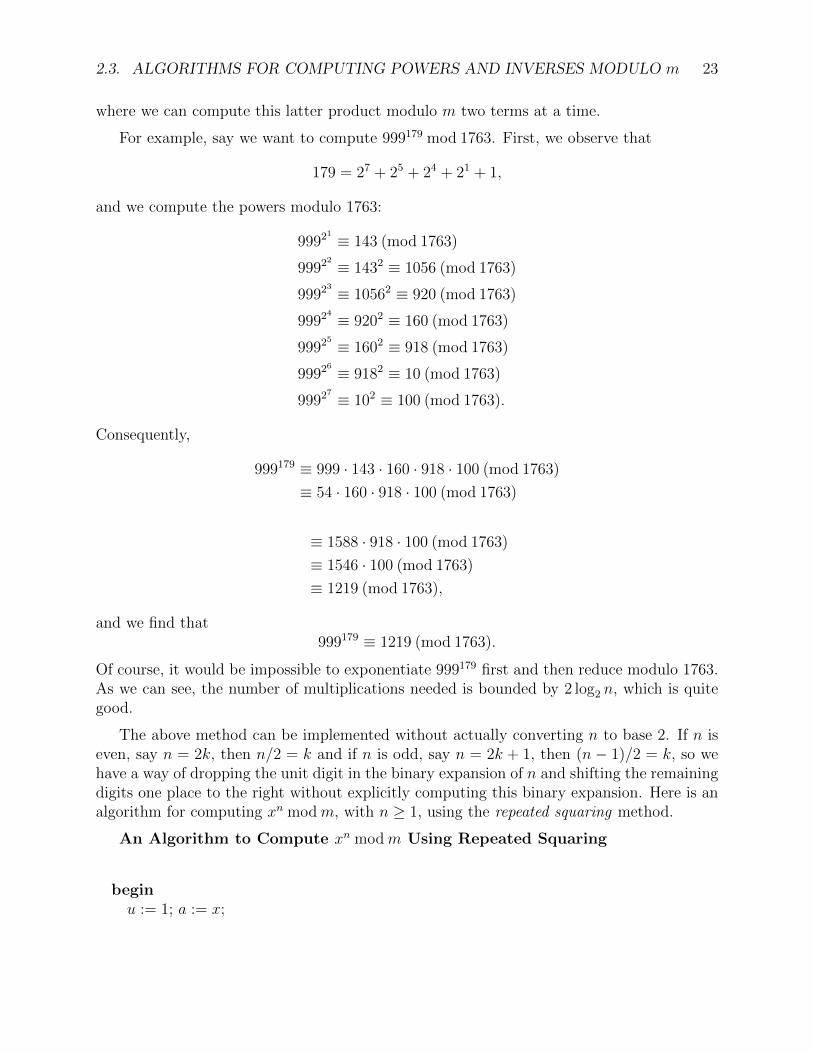
For example, say we want to compute 999179 mod 1763. First, we observe that
179 = 27 + 25 + 24 + 21 + 1,
and we compute the powers modulo 1763:
99921 ≡ 143 (mod 1763)
99922 ≡ 1432 ≡ 1056 (mod 1763)
99923 ≡ 10562 ≡ 920 (mod 1763)
99924 ≡ 9202 ≡ 160 (mod 1763)
99925 ≡ 1602 ≡ 918 (mod 1763)
99926 ≡ 9182 ≡ 10 (mod 1763)
99927 ≡ 102 ≡ 100 (mod 1763).
Consequently,
999179 ≡ 999 · 143 · 160 · 918 · 100 (mod 1763)
≡ 54 · 160 · 918 · 100 (mod 1763)
≡ 1588 · 918 · 100 (mod 1763)
≡ 1546 · 100 (mod 1763)
≡ 1219 (mod 1763),
and we find that999179 ≡ 1219 (mod 1763).
Of course, it would be impossible to exponentiate 999179 first and then reduce modulo 1763.As we can see, the number of multiplications needed is bounded by 2 log2 n, which is quitegood.
The above method can be implemented without actually converting n to base 2. If n iseven, say n = 2k, then n/2 = k and if n is odd, say n = 2k + 1, then (n − 1)/2 = k, so wehave a way of dropping the unit digit in the binary expansion of n and shifting the remainingdigits one place to the right without explicitly computing this binary expansion. Here is analgorithm for computing xn modm, with n ≥ 1, using the repeated squaring method.
An Algorithm to Compute xn modm Using Repeated Squaring
beginu := 1; a := x;

24 CHAPTER 2. PUBLIC KEY CRYPTOGRAPHY
while n > 1 doif even(n) then e := 0 else e := 1;if e = 1 then u := a · u mod m;a := a2 mod m; n := (n− e)/2
endwhile;u := a · u mod m
end
The final value of u is the result. The reason why the algorithm is correct is that after jrounds through the while loop, a = x2
jmodm and
u =∏
i∈J | i<j
x2i
modm,
with this product interpreted as 1 when j = 0.
Observe that the while loop is only executed n − 1 times to avoid squaring once moreunnecessarily and the last multiplication a ·u is performed outside of the while loop. Also, ifwe delete the reductions modulo m, the above algorithm is a fast method for computing thenth power of an integer x and the time speed-up of not performing the last squaring step ismore significant. We leave the details of the proof that the above algorithm is correct as anexercise.
Let us now consider the problem of computing efficiently the inverse of an integer a,modulo m, provided that gcd(a,m) = 1. Full details are given in Gallier [6], Chapter 5.
The extended Euclidean algorithm can be used to find some integers x, y, such that
ax+ by = gcd(a, b),
where a and b are any two positive integers. In our situation, a = m and b = a and we onlyneed to find y (we would like a positive integer).
When using the Euclidean algorithm for computing gcd(m, a), with 2 ≤ a < m, wecompute the following sequence of quotients and remainders.
m = aq1 + r1
a = r1q2 + r2
r1 = r2q3 + r3...
rk−1 = rkqk+1 + rk+1
...
rn−3 = rn−2qn−1 + rn−1
rn−2 = rn−1qn + 0,
2.3. ALGORITHMS FOR COMPUTING POWERS AND INVERSES MODULO m 25
with n ≥ 3, 0 < r1 < b, qk ≥ 1, for k = 1, . . . , n, and 0 < rk+1 < rk, for k = 1, . . . , n − 2.Observe that rn = 0. If n = 2, we have just two divisions,
m = aq1 + r1
a = r1q2 + 0,
with 0 < r1 < b, q1, q2 ≥ 1, and r2 = 0. Thus, it is convenient to set r−1 = m and r0 = a.
It can be shown (Gallier [6], Chapter 5) that if we set
x−1 = 1
y−1 = 0
x0 = 0
y0 = 1
xi+1 = xi−1 − xiqi+1
yi+1 = yi−1 − yiqi+1,
for i = 0, . . . , n− 2, then
mxn−1 + ayn−1 = gcd(m, a) = rn−1,
and so, if gcd(m, a) = 1, then rn−1 = 1 and we have
ayn−1 ≡ 1 (modm).
Now, yn−1 may be greater than m or negative but we already know how to deal with that.This suggests reducing modulo m during the recurrence and we are led to the followingrecurrence.
y−1 = 0
y0 = 1
zi+1 = yi−1 − yiqi+1
yi+1 = zi+1 modm if zi+1 ≥ 0
yi+1 = m− ((−zi+1) modm) if zi+1 < 0,
for i = 0, . . . , n− 2.
It is easy to prove by induction that
ayi ≡ ri (modm)
for i = 0, . . . , n − 1 and thus, if gcd(a,m) > 1, then a does not have an inverse modulo m,else
ayn−1 ≡ 1 (modm)
26 CHAPTER 2. PUBLIC KEY CRYPTOGRAPHY
and yn−1 is the inverse of a modulo m such that 1 ≤ yn−1 < m, as desired. Note that wealso get y0 = 1 when a = 1.
We leave this proof as an exercise. Here is an algorithm.
An Algorithm for Computing the Inverse of a Modulo m
Given any natural number a with 1 ≤ a < m and gcd(a,m) = 1, the following algorithmreturns the inverse of a modulo m as y.
beginy := 0; v := 1; g := m; r := a;pr := r; q := bg/prc; r := g − pr q; (divide g by pr, to get g = pr q + r)if r = 0 theny := 1; g := pr
elser = pr;while r 6= 0 dopr := r; pv := v;q := bg/prc; r := g − pr q; (divide g by pr, to get g = pr q + r)v := y − pv q;if v < 0 thenv := m− ((−v) mod m)
elsev = v mod m
endifg := pr; y := pv
endwhile;endif;inverse(a) := y
end
For example, we used the above algorithm to find that dA = 145, 604, 785 is the inverseof eA = 79921 modulo (pA − 1)(qA − 1) = 163, 251, 312.
The remaining issues are how to choose large random prime numbers p, q, and how tofind a random number e, which is relatively prime to (p − 1)(q − 1). For this, we rely on adeep result of number theory known as the prime number theorem.
2.4 Finding Large Primes; Signatures; Safety of RSA
Roughly speaking, the prime number theorem ensures that the density of primes is highenough to guarantee that there are many primes with a large specified number of digits.

2.4. FINDING LARGE PRIMES; SIGNATURES; SAFETY OF RSA 27
Figure 2.2: Pafnuty Lvovich Chebyshev, 1821–1894 (left), Jacques Salomon Hadamard,1865–1963 (middle), and Charles Jean de la Vallee Poussin, 1866–1962 (right)
The relevant function is the prime counting function π(n).
Definition 2.2. The prime counting function π is the function defined so that
π(n) = number of prime numbers p, such that p ≤ n,
for every natural number n ∈ N.
Obviously, π(0) = π(1) = 0. We have π(10) = 4 because the primes no greater than 10are 2, 3, 5, 7 and π(20) = 8 because the primes no greater than 20 are 2, 3, 5, 7, 11, 13, 17, 19.The growth of the function π was studied by Legendre, Gauss, Chebyshev, and Riemann
between 1808 and 1859. By then, it was conjectured that
π(n) ∼ n
ln(n), 1
for n large, which means that
limn7→∞
π(n)
/n
ln(n)= 1.
However, a rigorous proof was not found until 1896. Indeed, in 1896, Jacques Hadamardand Charles de la Vallee-Poussin independendly gave a proof of this “most wanted theorem,”using methods from complex analysis. These proofs are difficult and although more elemen-tary proofs were given later, in particular by Erdos and Selberg (1949), those proofs are stillquite hard. Thus, we content ourselves with a statement of the theorem.
Theorem 2.4. (Prime Number Theorem) For n large, the number of primes π(n) no largerthan n is approximately equal to n/ ln(n), which means that
limn7→∞
π(n)
/n
ln(n)= 1.
1We use ln(n) to denote the logarithm of n to the base e, known as the natural logarithm of n.
28 CHAPTER 2. PUBLIC KEY CRYPTOGRAPHY
Figure 2.3: Paul Erdos, 1913–1996 (left), Atle Selberg, 1917–2007 (right)
For a rather detailed account of the history of the prime number theorem (for short,PNT ), we refer the reader to Ribenboim [18] (Chapter 4).
As an illustration of the use of the PNT, we can estimate the number of primes with 200decimal digits. Indeed this is the difference of the number of primes up to 10200 minus thenumber of primes up to 10199, which is approximately
10200
200 ln 10− 10199
199 ln 10≈ 1.95 · 10197.
Thus, we see that there is a huge number of primes with 200 decimal digits. The number ofnatural numbers with 200 digits is 10200 − 10199 = 9 · 10199, thus the proportion of 200-digitnumbers that are prime is
1.95 · 10197
9 · 10199≈ 1
460.
Consequently, among the natural numbers with 200 digits, roughly one in every 460 is aprime.
Beware that the above argument is not entirely rigorous because the prime numbertheorem only yields an approximation of π(n) but sharper estimates can be used to say
how large n should be to guarantee a prescribed error on the probability, say 1%.
The implication of the above fact is that if we wish to find a random prime with 200digits, we pick at random some natural number with 200 digits and test whether it is prime.If this number is not prime, then we discard it and try again, and so on. On the average,after 460 trials, a prime should pop up,
This leads us the question: How do we test for primality?
Primality testing has also been studied for a long time. Remarkably, Fermat’s littletheorem yields a test for nonprimality. Indeed, if p > 1 fails to divide ap−1 − 1 for somenatural number a, where 2 ≤ a ≤ p − 1, then p cannot be a prime. The simplest a to tryis a = 2. From a practical point of view, we can compute ap−1 mod p using the method ofrepeated squaring and check whether the remainder is 1.

2.4. FINDING LARGE PRIMES; SIGNATURES; SAFETY OF RSA 29
Figure 2.4: Robert Daniel Carmichael, 1879–1967
But what if p fails the Fermat test? Unfortunately, there are natural numbers p, suchthat p divides 2p−1 − 1 and yet, p is composite. For example p = 341 = 11 · 31 is such anumber.
Actually, 2340 being quite big, how do we check that 2340 − 1 is divisible by 341?
We just have to show that 2340 − 1 is divisible by 11 and by 31. We can use Fermat’slittle theorem. Because 11 is prime, we know that 11 divides 210 − 1. But,
2340 − 1 = (210)34 − 1 = (210 − 1)((210)33 + (210)32 + · · ·+ 1),
so 2340 − 1 is also divisible by 11.
As to divisibility by 31, observe that 31 = 25 − 1, and
2340 − 1 = (25)68 − 1 = (25 − 1)((25)67 + (25)66 + · · ·+ 1),
so 2340 − 1 is also divisible by 31.
A number p that is not a prime but behaves like a prime in the sense that p divides2p−1 − 1, is called a pseudo-prime. Unfortunately, the Fermat test gives a “false positive”for pseudo-primes.
Rather than simply testing whether 2p−1 − 1 is divisible by p, we can also try whether3p−1 − 1 is divisible by p and whether 5p−1 − 1 is divisible by p, and so on.
Unfortunately, there are composite natural numbers p, such that p divides ap−1 − 1, forall positive natural numbers a with gcd(a, p) = 1. Such numbers are known as Carmichaelnumbers . The smallest Carmichael number is p = 561 = 3 · 11 · 17. The reader should tryproving that, in fact, a560 − 1 is divisible by 561 for every positive natural number a, suchthat gcd(a, 561) = 1, using the technique that we used to prove that 341 divides 2340 − 1.
It turns out that there are infinitely many Carmichael numbers. Again, for a thoroughintroduction to primality testing, pseudo-primes, Carmichael numbers, and more, we highlyrecommend Ribenboim [18] (Chapter 2). An excellent (but more terse) account is also givenin Koblitz [10] (Chapter V).

30 CHAPTER 2. PUBLIC KEY CRYPTOGRAPHY
Still, what do we do about the problem of false positives? The key is to switch toprobabilistic methods . Indeed, if we can design a method that is guaranteed to give a falsepositive with probablity less than 0.5, then we can repeat this test for randomly chosenas and reduce the probability of false positive considerably. For example, if we repeat theexperiment 100 times, the probability of false positive is less than 2−100 < 10−30. This isprobably less than the probability of hardware failure.
Various probabilistic methods for primality testing have been designed. One of them is theMiller–Rabin test, another the APR test, and yet another the Solovay–Strassen test. Since2002, it has been known that primality testing can be done in polynomial time. This resultis due to Agrawal, Kayal, and Saxena and known as the AKS test solved a long-standingproblem; see Dietzfelbinger [4] and Crandall and Pomerance [3] (Chapter 4). Remarkably,Agrawal and Kayal worked on this problem for their senior project in order to complete theirbachelor’s degree. It remains to be seen whether this test is really practical for very largenumbers.
A very important point to make is that these primality testing methods do not provide afactorization of m when m is composite. This is actually a crucial ingredient for the securityof the RSA scheme. So far, it appears (and it is hoped) that factoring an integer is a muchharder problem than testing for primality and all known methods are incapable of factoringnatural numbers with over 300 decimal digits (it would take centuries).
For a comprehensive exposition of the subject of primality-testing, we refer the reader toCrandall and Pomerance [3] (Chapters 3 and 4) and again, to Ribenboim [18] (Chapter 2)and Koblitz [10] (Chapter V). We give a thorough presentation of the Miller–Rabin and theSolovay–Strassen tests in Chapters 5 and 6 (with complete proofs).
Going back to the RSA method, we now have ways of finding the large random primesp and q by picking at random some 200-digit numbers and testing for primality. Rivest,Shamir, and Adleman also recommend to pick p and q so that they differ by a few decimaldigits, that both p−1 and q−1 should contain large prime factors and that gcd(p−1, q−1)should be small. The public key, e, relatively prime to (p − 1)(q − 1) can also be foundby a similar method: Pick at random a number, e < (p − 1)(q − 1), which is large enough(say, greater than maxp, q) and test whether gcd(e, (p− 1)(q− 1)) = 1, which can be donequickly using the extended Euclidean algorithm. If not, discard e and try another number,and so on. It is easy to see that such an e will be found in no more trials than it takes tofind a prime; see Lovasz, Pelikan, and Vesztergombi [13] (Chapter 15), which contains one ofthe simplest and clearest presentations of RSA that we know of. Koblitz [10] (Chapter IV)also provides some details on this topic as well as Menezes, van Oorschot, and Vanstone’sHandbook [14].
If Albert receives a message coming from Julia, how can he be sure that this messagedoes not come from an imposter? Just because the message is signed “Julia” does not meanthat it comes from Julia; it could have been sent by someone else pretending to be Julia,inasmuch as all that is needed to send a message to Albert is Albert’s public key, which isknown to everybody. This leads us to the issue of signatures .

2.4. FINDING LARGE PRIMES; SIGNATURES; SAFETY OF RSA 31
There are various schemes for adding a signature to an encrypted message to ensure thatthe sender of a message is really who he or she claims to be (with a high degree of confidence).The trick is to make use of the sender’s keys. We propose two scenarios.
1. The sender, Julia, encrypts the message x to be sent with her own private key , (dJ ,mJ),creating the message DJ(x) = y1. Then, Julia adds her signature, “Julia”, at the endof the message y1, encrypts the message “y1 Julia” using Albert’s public key , (eA,mA),creating the message y2 = EA(y1 Julia), and finally sends the message y2 to Albert.
When Albert receives the encrypted message y2 claiming to come from Julia, first hedecrypts the message using his private key (dA,mA). He will see an encrypted message,DA(y2) = y1 Julia, with the legible signature, Julia. He will then delete the signaturefrom this message and decrypt the message y1 using Julia’s public key (eJ ,mJ), gettingx = EJ(y1). Albert will know whether someone else faked this message if the resultis garbage. Indeed, only Julia could have encrypted the original message x with herprivate key, which is only known to her. An eavesdropper who is pretending to beJulia would not know Julia’s private key and so, would not have encrypted the originalmessage to be sent using Julia’s secret key.
2. The sender, Julia, first adds her signature, “Julia”, to the message x to be sent andthen, she encrypts the message “x Julia” with Albert’s public key (eA,mA), creatingthe message y1 = EA(x Julia). Julia also encrypts the original message x using herprivate key (dJ ,mJ) creating the message y2 = DJ(x), and finally she sends the pairof messages (y1, y2).
When Albert receives a pair of messages (y1, y2), claiming to have been sent by Julia,first Albert decrypts y1 using his private key (dA,mA), getting the message DA(y1) =x Julia. Albert finds the signature, Julia, and then decrypts y2 using Julia’s public key(eJ ,mJ), getting the message x′ = EJ(y2). If x = x′, then Albert has serious assurancethat the sender is indeed Julia and not an imposter.
The last topic that we would like to discuss is the security of the RSA scheme. This is adifficult issue and many researchers have worked on it. As we remarked earlier, the securityof RSA hinges on the fact that factoring is hard. It has been shown that if one has a methodfor breaking the RSA scheme (namely, to find the secret key d), then there is a probabilisticmethod for finding the factors p and q, of m = pq (see Koblitz [10], Chapter IV, Section 2,or Menezes, van Oorschot, and Vanstone [14], Section 8.2.2). If p and q are chosen to belarge enough, factoring m = pq will be practically impossible and so it is unlikely that RSAcan be cracked. However, there may be other attacks and, at present, there is no proof thatRSA is fully secure.
Observe that because m = pq is known to everybody, if somehow one can learn N =(p−1)(q−1), then p and q can be recovered. Indeed N = (p−1)(q−1) = pq− (p+ q) + 1 =

32 CHAPTER 2. PUBLIC KEY CRYPTOGRAPHY
m− (p+ q) + 1 and so,
pq = m
p+ q = m−N + 1,
and p and q are the roots of the quadratic equation
X2 − (m−N + 1)X +m = 0.
Thus, a line of attack is to try to find the value of (p− 1)(q − 1). For more on the securityof RSA, see Menezes, van Oorschot, and Vanstone’s Handbook [14].

Chapter 3
Primality Testing Using RandomizedAlgorithms; Introduction
In article 329 of his famous Disquisitiones Arithmeticae [7] (published in 1801, when he was24 years old), C.F. Gauss writes (in Latin!):
“The problem of distinguishing prime numbers from composite numbers andresolving the latter into their prime factors is known to be one of the mostimportant and useful in arithmetic. It has engaged the industry and wisdom ofancient and moderm geometers to such an extent that it would be superfluous todiscuss the problem at length. Nevertherless we must confess that all methodsthat have been proposed thus far are either restricted to very special cases or areso laborious and difficult that even for numbers that do not exceed the limits oftables constructed by estimable men, they try the patience of even the practicedcalculator. And these methods do not apply at all to larger numbers ... Thetechniques that were previously known would require intolerable labor even forthe most indefatigable calculator.”
The problem of determining whether a given integer is prime is one of the better knownand most easily understood problems of pure mathematics. This problem has caught theinterest of mathematicians again and again for centuries. However, it was not until the 20thcentury that questions about primality testing and factoring were recognized as problemsof practical importance, and a central part of applied mathematics. The advent of cryp-tographic systems that use large primes, such as RSA, was the main driving force for thedevelopment of fast and reliable methods for primality testing. Indeed, as we saw in ear-lier sections of these notes, in order to create RSA keys, one needs to produce large primenumbers. How do we do that?
One method is to produce a random string of digits (say of 200 digits), and then totest whether this number is prime or not. As we explained earlier, by the Prime NumberTheorem, among the natural numbers with 200 digits, roughly one in every 460 is a prime.Thus, it should take at most 460 trials (picking at random some natural number with 200
33

34 CHAPTER 3. PRIMALITY TESTING USING RANDOMIZED ALGORITHMS
digits) before a prime shows up. Note that we need a mechanism to generate randomnumbers, an interesting and tricky problem, but for now, we postpone discussing randomnumber generation.
It remains to find methods for testing an integer for primality, and perhaps for factoringcomposite numbers.
In 1903, at the meeting of the American Mathematical Society, F.N. Cole came to theblackboard and, without saying a word, wrote down
267 − 1 = 147573952589676412927 = 193707721× 761838257287,
and then used long multiplication to multiply the two numbers on the right-hand side toprove that he was indeed correct. Afterwards, he said that figuring this out had taken him“three years of Sundays.” Too bad laptops did not exist in 1903.
The moral of this tale is that checking that a number is composite can be done quickly(that is, in polynomial time), but finding a factorization is hard. In general, it requires anexhaustive search. Another important observation is that most efficient tests for composite-ness do not produce a factorization. For example, Lucas had already shown that 267 − 1 iscomposite, but without finding a factor.
In fact, although this has not been proved, factoring appears to be a much harder problemthan primality testing, which is a good thing since the safety of many cryptographic systemsdepends on the assumption that factoring is hard!
As we explained in the introduction, most algorithms for testing whether an integer nis prime actually test for compositeness. This is because tests for compositeness usuallytry to find a counterexample to some property, say A, implied by primality. If such acounterexample can be guessed, then it is cheap to check that property A fails, and thenwe know for sure that n is composite. We also have a witness (or certificate) that n iscomposite. If the algorithm fails to show that n is composite, does this imply that n isprime? Unfortunately, no. This is because, in general, the algorithm has not tested allpotential countexamples. So, how do we fix the algorithm?
One possibility is to try systematically all potential countexamples. If the algorithm failson all counterexamples, then the number n has to be prime. The problem with this approachis that the number of counterexamples is generally too big, and this method is not practical.Methods of this kind are presented in Crandall and Pomerance [3] and Ribenboim [18].
Another approach is to use a randomized algorithm. Typically, a counterexample is somenumber a randomly chosen from the set 2, . . . , n − 2, and the algorithm performs a teston a and n to determine whether a is a counterexample. If the test is positive, then for suren is composite, and a is a witness to the fact that n is composite. If the test is negative,then the algorithm does not find n to be composite, and we can call it again several times,each time picking (independently from previous trials) another random number a. If thealgorithm ever reports a positive test, then for sure n is a composite. But what if we call the

35
algorithm say 20 times, and every time the test is negative (which means that the algorithmdoes not find n to be composite 20 times). Can we be sure that n is a prime?
Not necessarily, because the test performed by the algorithm may not be 100% reliable.If n is prime, the test performed by the algorithm on every a is negative (as it should), butthere may be some composite n and some a for which the test is negative. Such a number a iscalled a liar , because it fools the test. Even though n is composite, a does not trigger the testto be positive, to indicate that n is indeed composite. But if the conditional probability thatthe test performed by the algorithm is positive given that n is composite is large enough, sayat least 1/2, then it can be shown that the conditional probability that n is composite, giventhat the test performed by the algorithm is negative 20 times, is less than ln(n) · (1/2)20 (seeSection 5.4).1 In summary, if we run the algorithm ` times (for ` large enough, say ` = 100)
on some number n, and if each time the test performed by the algorithm is negative, thenwe can be very confident that n is prime. Such kind of randomized algorithm is called aMonte Carlo algorithm.
Several randomized algorithms for primality testing have been designed, including theMiller–Rabin and the Solovay–Strassen tests, to be discussed in Chapters 5 and 6. Then,in the summer of 2002, a paper with the title “PRIMES is in P,” by Agrawal, Kayal andSaxena, appeared on the website of the Indian Institute of Technology at Kanpur, India.In this paper, it was shown that testing for primality has a deterministic (nonrandomized)algorithm that runs in polynomial time. Finally, the long-standing open problem of “decidingwhether primality testing is in P” was settled in this amazing paper, by an algorithm usuallyreferred to as the AKS algorithm. We will not discuss this algorithm in these notes (but,perhaps in another set of notes ...).
1Recall that we use ln(n) to denote the logarithm of n to the base e, known as the natural logarithm of n.
36 CHAPTER 3. PRIMALITY TESTING USING RANDOMIZED ALGORITHMS

Chapter 4
Basic Facts About Groups, Rings,Fields, and Number Theory
This chapter provides a review of the mathematical background needed to thoroughly under-stand the randomized algorithms for primality testing presented in the following chapters,especially the proofs. This includes some basics on groups, the structure of cyclic groups,rings, fields, and finite fields. The multiplicative groups (Z/nZ)∗ of invertible elements of therings Z/nZ play a particularly important role. It is crucial to know when the group (Z/nZ)∗
is cyclic, which means that it is generated by a single element called a primitive root . Afamous result due to Gauss says that the group (Z/nZ)∗ has a primitive root iff n = 2, 4, pm,or 2pm where p is an odd prime. We give a complete proof of this result in Sections 4.4 and4.5.
Readers familiar with groups, rings and fields should probably skip Sections 4.1, 4.2, and4.3. However, the reader may want to read Sections 4.4 and 4.5, skipping proofs the firsttime, before reading Chapter 5. The material in these two sections is classical and verybeautiful. Similarly, the reader may want to read Section 4.7, omitting proofs the first time,before reading Chapter 6.
4.1 Groups, Subgroups, Cosets
Definition 4.1. A group is a set G equipped with a binary operation · : G × G → G thatassociates an element a · b ∈ G to every pair of elements a, b ∈ G, and having the followingproperties: · is associative, has an identity element e ∈ G, and every element in G is invertible(w.r.t. ·). More explicitly, this means that the following equations hold for all a, b, c ∈ G:
(G1) a · (b · c) = (a · b) · c. (associativity);
(G2) a · e = e · a = a. (identity);
(G3) For every a ∈ G, there is some a−1 ∈ G such that a · a−1 = a−1 · a = e. (inverse).
37

38 CHAPTER 4. BASIC FACTS ABOUT GROUPS, AND NUMBER THEORY
A group G is abelian (or commutative) if
a · b = b · a for all a, b ∈ G.
A set M together with an operation · : M ×M → M and an element e satisfying onlyConditions (G1) and (G2) is called a monoid . For example, the set N = 0, 1, . . . , n, . . . ofnatural numbers is a (commutative) monoid under addition. However, it is not a group.
Some examples of groups are given below.
Example 4.1.
1. The set Z = . . . ,−n, . . . ,−1, 0, 1, . . . , n, . . . of integers is an abelian group underaddition, with identity element 0. However, Z∗ = Z − 0 is not a group undermultiplication.
2. The set Q of rational numbers (fractions p/q with p, q ∈ Z and q 6= 0) is an abeliangroup under addition, with identity element 0. The set Q∗ = Q−0 is also an abeliangroup under multiplication, with identity element 1.
3. Given any nonempty set S, the set of bijections f : S → S, also called permutationsof S, is a group under function composition (i.e., the multiplication of f and g is thecomposition g f), with identity element the identity function idS. This group is notabelian as soon as S has more than two elements. The permutation group of the setS = 1, . . . , n is often denoted Sn and called the symmetric group on n elements.
4. For any natural number n ≥ 1, the set Z/nZ of residues modulo n as in Definition 2.1is an abelian group under addition modulo n.
5. The set of n×n invertible matrices with real (or complex) coefficients is a group undermatrix multiplication, with identity element the identity matrix In. This group iscalled the general linear group and is usually denoted by GL(n,R) (or GL(n,C)).
6. The set of n × n invertible matrices A with real (or complex) coefficients such thatdet(A) = 1 is a group under matrix multiplication, with identity element the identitymatrix In. This group is called the special linear group and is usually denoted bySL(n,R) (or SL(n,C)).
7. The set of n× n matrices Q with real coefficients such that
QQ> = Q>Q = In
is a group under matrix multiplication, with identity element the identity matrix In;we have Q−1 = Q>. This group is called the orthogonal group and is usually denotedby O(n).
4.1. GROUPS, SUBGROUPS, COSETS 39
8. The set of n× n invertible matrices Q with real coefficients such that
QQ> = Q>Q = In and det(Q) = 1
is a group under matrix multiplication, with identity element the identity matrix In;as in (6), we have Q−1 = Q>. This group is called the special orthogonal group orrotation group and is usually denoted by SO(n).
The groups in (5)–(8) are nonabelian for n ≥ 2, except for SO(2) which is abelian (but O(2)is not abelian).
It is customary to denote the operation of an abelian group G by +, in which case theinverse a−1 of an element a ∈ G is denoted by −a.
The identity element of a group is unique. In fact, we can prove a more general fact:
Proposition 4.1. If a binary operation · : M ×M → M is associative and if e′ ∈ M is aleft identity and e′′ ∈M is a right identity, which means that
e′ · a = a for all a ∈M (G2l)
anda · e′′ = a for all a ∈M, (G2r)
then e′ = e′′.
Proof. If we let a = e′′ in equation (G2l), we get
e′ · e′′ = e′′,
and if we let a = e′ in equation (G2r), we get
e′ · e′′ = e′,
and thuse′ = e′ · e′′ = e′′,
as claimed.
Proposition 4.1 implies that the identity element of a monoid is unique, and since everygroup is a monoid, the identity element of a group is unique. Furthermore, every element ina group has a unique inverse. This is a consequence of a slightly more general fact:
Proposition 4.2. In a monoid M with identity element e, if some element a ∈M has someleft inverse a′ ∈M and some right inverse a′′ ∈M , which means that
a′ · a = e (G3l)
anda · a′′ = e, (G3r)
then a′ = a′′.

40 CHAPTER 4. BASIC FACTS ABOUT GROUPS, AND NUMBER THEORY
Proof. Using (G3l) and the fact that e is an identity element, we have
(a′ · a) · a′′ = e · a′′ = a′′.
Similarly, Using (G3r) and the fact that e is an identity element, we have
a′ · (a · a′′) = a′ · e = a′.
However, since M is monoid, the operation · is associative, so
a′ = a′ · (a · a′′) = (a′ · a) · a′′ = a′′,
as claimed.
Remark: Axioms (G2) and (G3) can be weakened a bit by requiring only (G2r) (the exis-tence of a right identity) and (G3r) (the existence of a right inverse for every element) (or(G2l) and (G3l)). It is a good exercise to prove that the group axioms (G2) and (G3) followfrom (G2r) and (G3r).
Definition 4.2. If a group G has a finite number n of elements, we say that G is a groupof order n. If G is infinite, we say that G has infinite order . The order of a group is usuallydenoted by |G| (if G is finite).
Given a group G, for any two subsets R, S ⊆ G, we let
RS = r · s | r ∈ R, s ∈ S.
In particular, for any g ∈ G, if R = g, we write
gS = g · s | s ∈ S,
and similarly, if S = g, we write
Rg = r · g | r ∈ R.
From now on, we will drop the multiplication sign and write g1g2 for g1 · g2.
Definition 4.3. Let G be a group. For any g ∈ G, define Lg, the left translation by g, byLg(a) = ga, for all a ∈ G, and Rg, the right translation by g, by Rg(a) = ag, for all a ∈ G.
The following simple fact is often used.
Proposition 4.3. Given a group G, the translations Lg and Rg are bijections.
Proof. We show this for Lg, the proof for Rg being similar.
If Lg(a) = Lg(b), then ga = gb, and multiplying on the left by g−1, we get a = b, so Lginjective. For any b ∈ G, we have Lg(g
−1b) = gg−1b = b, so Lg is surjective. Therefore, Lgis bijective.
4.1. GROUPS, SUBGROUPS, COSETS 41
Definition 4.4. Given a group G, a subset H of G is a subgroup of G iff
(1) The identity element e of G also belongs to H (e ∈ H);
(2) For all h1, h2 ∈ H, we have h1h2 ∈ H;
(3) For all h ∈ H, we have h−1 ∈ H.
The proof of the following proposition is left as an exercise.
Proposition 4.4. Given a group G, a subset H ⊆ G is a subgroup of G iff H is nonemptyand whenever h1, h2 ∈ H, then h1h
−12 ∈ H.
If the group G is finite, then the following criterion can be used.
Proposition 4.5. Given a finite group G, a subset H ⊆ G is a subgroup of G iff
(1) e ∈ H;
(2) H is closed under multiplication.
Proof. We just have to prove that Condition (3) of Definition 4.4 holds. For any a ∈ H,since the left translation La is bijective, its restriction to H is injective, and since H is finite,it is also bijective. Since e ∈ H, there is a unique b ∈ H such that La(b) = ab = e. However,if a−1 is the inverse of a in G, we also have La(a
−1) = aa−1 = e, and by injectivity of La, wehave a−1 = b ∈ H.
Example 4.2.
1. For any integer n ∈ Z, the set
nZ = nk | k ∈ Z
is a subgroup of the group Z.
2. The set of matrices
GL+(n,R) = A ∈ GL(n,R) | det(A) > 0
is a subgroup of the group GL(n,R).
3. The group SL(n,R) is a subgroup of the group GL(n,R).
4. The group O(n) is a subgroup of the group GL(n,R).
5. The group SO(n) is a subgroup of the group O(n), and a subgroup of the groupSL(n,R).
42 CHAPTER 4. BASIC FACTS ABOUT GROUPS, AND NUMBER THEORY
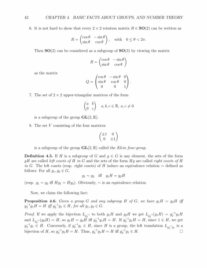
6. It is not hard to show that every 2× 2 rotation matrix R ∈ SO(2) can be written as
R =
(cos θ − sin θsin θ cos θ
), with 0 ≤ θ < 2π.
Then SO(2) can be considered as a subgroup of SO(3) by viewing the matrix
R =
(cos θ − sin θsin θ cos θ
)as the matrix
Q =
cos θ − sin θ 0sin θ cos θ 0
0 0 1
.
7. The set of 2× 2 upper-triangular matrices of the form(a b0 c
)a, b, c ∈ R, a, c 6= 0
is a subgroup of the group GL(2,R).
8. The set V consisting of the four matrices(±1 00 ±1
)is a subgroup of the group GL(2,R) called the Klein four-group.
Definition 4.5. If H is a subgroup of G and g ∈ G is any element, the sets of the formgH are called left cosets of H in G and the sets of the form Hg are called right cosets of Hin G. The left cosets (resp. right cosets) of H induce an equivalence relation ∼ defined asfollows: For all g1, g2 ∈ G,
g1 ∼ g2 iff g1H = g2H
(resp. g1 ∼ g2 iff Hg1 = Hg2). Obviously, ∼ is an equivalence relation.
Now, we claim the following fact:
Proposition 4.6. Given a group G and any subgroup H of G, we have g1H = g2H iffg−12 g1H = H iff g−12 g1 ∈ H, for all g1, g2 ∈ G.
Proof. If we apply the bijection Lg−12
to both g1H and g2H we get Lg−12
(g1H) = g−12 g1H
and Lg−12
(g2H) = H, so g1H = g2H iff g−12 g1H = H. If g−12 g1H = H, since 1 ∈ H, we get
g−12 g1 ∈ H. Conversely, if g−12 g1 ∈ H, since H is a group, the left translation Lg−12 g1
is a
bijection of H, so g−12 g1H = H. Thus, g−12 g1H = H iff g−12 g1 ∈ H.
4.1. GROUPS, SUBGROUPS, COSETS 43
It follows that the equivalence class of an element g ∈ G is the coset gH (resp. Hg).Since Lg is a bijection between H and gH, the cosets gH all have the same cardinality. Themap Lg−1 Rg is a bijection between the left coset gH and the right coset Hg, so they alsohave the same cardinality. Since the distinct cosets gH form a partition of G, we obtain thefollowing fact:
Proposition 4.7. (Lagrange) For any finite group G and any subgroup H of G, the orderh of H divides the order n of G.
Definition 4.6. Given a finite group G and a subgroup H of G, if n = |G| and h = |H|,then the ratio n/h is denoted by (G : H) and is called the index of H in G.
The index (G : H) is the number of left (and right) cosets of H in G. Proposition 4.7can be stated as
|G| = (G : H)|H|.
The set of left cosets of H in G (which, in general, is not a group) is denoted G/H.The “points” of G/H are obtained by “collapsing” all the elements in a coset into a singleelement.
Example 4.3.
1. Let n be any positive integer, and consider the subgroup nZ of Z (under addition).The coset of 0 is the set 0, and the coset of any nonzero integer m ∈ Z is
m+ nZ = m+ nk | k ∈ Z.
By dividing m by n, we have m = nq + r for some unique r such that 0 ≤ r ≤ n− 1.But then we see that r is the smallest positive element of the coset m + nZ. Thisimplies that there is a bijection betwen the cosets of the subgroup nZ of Z and the setof residues 0, 1, . . . , n− 1 modulo n, or equivalently a bijection with Z/nZ.
2. The cosets of SL(n,R) in GL(n,R) are the sets of matrices
ASL(n,R) = AB | B ∈ SL(n,R), A ∈ GL(n,R).
Since A is invertible, det(A) 6= 0, and we can write A = (det(A))1/n((det(A))−1/nA)if det(A) > 0 and A = (− det(A))1/n((− det(A))−1/nA) if det(A) < 0. But we have(det(A))−1/nA ∈ SL(n,R) if det(A) > 0 and −(− det(A))−1/nA ∈ SL(n,R) if det(A) <0, so the coset ASL(n,R) contains the matrix
(det(A))1/nIn if det(A) > 0, −(− det(A))1/nIn if det(A) < 0.
It follows that there is a bijection between the cosets of SL(n,R) in GL(n,R) and R.
44 CHAPTER 4. BASIC FACTS ABOUT GROUPS, AND NUMBER THEORY
3. The cosets of SO(n) in GL+(n,R) are the sets of matrices
ASO(n) = AQ | Q ∈ SO(n), A ∈ GL+(n,R).
It can be shown (using the polar form for matrices) that there is a bijection betweenthe cosets of SO(n) in GL+(n,R) and the set of n × n symmetric, positive, definitematrices; these are the symmetric matrices whose eigenvalues are strictly positive.
4. The cosets of SO(2) in SO(3) are the sets of matrices
QSO(2) = QR | R ∈ SO(2), Q ∈ SO(3).
The group SO(3) moves the points on the sphere S2 in R3, namely for any x ∈ S2,
x 7→ Qx for any rotation Q ∈ SO(3).
Here,S2 = (x, y, z) ∈ R3 | x2 + y2 + z2 = 1.
Let N = (0, 0, 1) be the north pole on the sphere S2. Then it is not hard to show thatSO(2) is precisely the subgroup of SO(3) that leaves N fixed. As a consequence, allrotations QR in the coset QSO(2) map N to the same point QN ∈ S2, and it can beshown that there is a bijection between the cosets of SO(2) in SO(3) and the pointson S2. The surjectivity of this map has to do with the fact that the action of SO(3)on S2 is transitive, which means that for any point x ∈ S2, there is some rotationQ ∈ SO(3) such that QN = x.
It is tempting to define a multiplication operation on left cosets (or right cosets) bysetting
(g1H)(g2H) = (g1g2)H,
but this operation is not well defined in general, unless the subgroup H possesses a specialproperty. In Example 4.3, it is possible to define multiplication of cosets in (1), but it is notpossible in (2) and (3).
The property of the subgroup H that allows defining a multiplication operation on leftcosets is typical of the kernels of group homomorphisms, so we are led to the followingdefinition.
Definition 4.7. Given any two groups G and G′, a function ϕ : G→ G′ is a homomorphismiff
ϕ(g1g2) = ϕ(g1)ϕ(g2), for all g1, g2 ∈ G.
Taking g1 = g2 = e (in G), we see that
ϕ(e) = e′,
and taking g1 = g and g2 = g−1, we see that
ϕ(g−1) = (ϕ(g))−1.

4.1. GROUPS, SUBGROUPS, COSETS 45
Example 4.4.
1. The map ϕ : Z→ Z/nZ given by ϕ(m) = m mod n for all m ∈ Z is a homomorphism.
2. The map det : GL(n,R) → R is a homomorphism because det(AB) = det(A) det(B)for any two matrices A,B. Similarly, the map det : O(n)→ R is a homomorphism.
If ϕ : G → G′ and ψ : G′ → G′′ are group homomorphisms, then ψ ϕ : G → G′′ is alsoa homomorphism. If ϕ : G→ G′ is a homomorphism of groups, and if H ⊆ G, H ′ ⊆ G′ aretwo subgroups, then it is easily checked that
Im H = ϕ(H) = ϕ(g) | g ∈ H
is a subgroup of G′ andϕ−1(H ′) = g ∈ G | ϕ(g) ∈ H ′
is a subgroup of G. In particular, when H ′ = e′, we obtain the kernel , Ker ϕ, of ϕ.
Definition 4.8. If ϕ : G → G′ is a homomorphism of groups, and if H ⊆ G is a subgroupof G, then the subgroup of G′,
Im H = ϕ(H) = ϕ(g) | g ∈ H,
is called the image of H by ϕ, and the subgroup of G,
Ker ϕ = g ∈ G | ϕ(g) = e′,
is called the kernel of ϕ.
Example 4.5.
1. The kernel of the homomorphism ϕ : Z→ Z/nZ is nZ.
2. The kernel of the homomorphism det : GL(n,R)→ R is SL(n,R). Similarly, the kernelof the homomorphism det : O(n)→ R is SO(n).
The following characterization of the injectivity of a group homomorphism is used all thetime.
Proposition 4.8. If ϕ : G→ G′ is a homomorphism of groups, then ϕ : G→ G′ is injectiveiff Ker ϕ = e. (We also write Ker ϕ = (0).)
Proof. Assume ϕ is injective. Since ϕ(e) = e′, if ϕ(g) = e′, then ϕ(g) = ϕ(e), and byinjectivity of ϕ we must have g = e, so Ker ϕ = e.
Conversely, assume that Ker ϕ = e. If ϕ(g1) = ϕ(g2), then by multiplication on theleft by (ϕ(g1))
−1 we get
e′ = (ϕ(g1))−1ϕ(g1) = (ϕ(g1))
−1ϕ(g2),

46 CHAPTER 4. BASIC FACTS ABOUT GROUPS, AND NUMBER THEORY
and since ϕ is a homomorphism (ϕ(g1))−1 = ϕ(g−11 ), so
e′ = (ϕ(g1))−1ϕ(g2) = ϕ(g−11 )ϕ(g2) = ϕ(g−11 g2).
This shows that g−11 g2 ∈ Ker ϕ, but since Ker ϕ = e we have g−11 g2 = e, and thus g2 = g1,proving that ϕ is injective.
Definition 4.9. We say that a group homomorphism ϕ : G→ G′ is an isomorphism if thereis a homomorphism ψ : G′ → G, so that
ψ ϕ = idG and ϕ ψ = idG′ . (†)
If ϕ is an isomorphism we say that the groups G and G′ are isomorphic. When G′ = G, agroup isomorphism is called an automorphism.
The reasoning used in the proof of Proposition 4.2 shows that if a a group homomorphismϕ : G→ G′ is an isomorphism, then the homomorphism ψ : G′ → G satisfying Condition (†)is unique. This homomorphism is denoted ϕ−1.
The left translations Lg and the right translations Rg are automorphisms of G.
Suppose ϕ : G → G′ is a bijective homomorphism, and let ϕ−1 be the inverse of ϕ (as afunction). Then for all a, b ∈ G, we have
ϕ(ϕ−1(a)ϕ−1(b)) = ϕ(ϕ−1(a))ϕ(ϕ−1(b)) = ab,
and soϕ−1(ab) = ϕ−1(a)ϕ−1(b),
which proves that ϕ−1 is a homomorphism. Therefore, we proved the following fact.
Proposition 4.9. A bijective group homomorphism ϕ : G→ G′ is an isomorphism.
Observe that the property
gH = Hg, for all g ∈ G. (∗)
is equivalent by multiplication on the right by g−1 to
gHg−1 = H, for all g ∈ G,
and the above is equivalent to
gHg−1 ⊆ H, for all g ∈ G. (∗∗)
This is because gHg−1 ⊆ H implies H ⊆ g−1Hg, and this for all g ∈ G.
Proposition 4.10. Let ϕ : G → G′ be a group homomorphism. Then H = Ker ϕ satisfiesProperty (∗∗), and thus Property (∗).

4.1. GROUPS, SUBGROUPS, COSETS 47
Proof. We have
ϕ(ghg−1) = ϕ(g)ϕ(h)ϕ(g−1) = ϕ(g)e′ϕ(g)−1 = ϕ(g)ϕ(g)−1 = e′,
for all h ∈ H = Ker ϕ and all g ∈ G. Thus, by definition of H = Ker ϕ, we have gHg−1 ⊆H.
Definition 4.10. For any group G, a subgroup N of G is a normal subgroup of G iff
gNg−1 = N, for all g ∈ G.
This is denoted by N CG.
Proposition 4.10 shows that the kernel Ker ϕ of a homomorphism ϕ : G→ G′ is a normalsubgroup of G.
Observe that if G is abelian, then every subgroup of G is normal.
Consider Example 4.2. Let R ∈ SO(2) and A ∈ SL(2,R) be the matrices
R =
(0 −11 0
), A =
(1 10 1
).
Then
A−1 =
(1 −10 1
)and we have
ARA−1 =
(1 10 1
)(0 −11 0
)(1 −10 1
)=
(1 −11 0
)(1 −10 1
)=
(1 −21 −1
),
and clearly ARA−1 /∈ SO(2). Therefore SO(2) is not a normal subgroup of SL(2,R). Thesame counter-example shows that O(2) is not a normal subgroup of GL(2,R).
Let R ∈ SO(2) and Q ∈ SO(3) be the matrices
R =
0 −1 01 0 00 0 1
, Q =
1 0 00 0 −10 1 0
.
Then
Q−1 = Q> =
1 0 00 0 10 −1 0
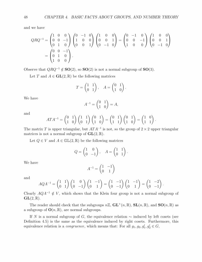
48 CHAPTER 4. BASIC FACTS ABOUT GROUPS, AND NUMBER THEORY
and we have
QRQ−1 =
1 0 00 0 −10 1 0
0 −1 01 0 00 0 1
1 0 00 0 10 −1 0
=
0 −1 00 0 −11 0 0
1 0 00 0 10 −1 0
=
0 0 −10 1 01 0 0
.
Observe that QRQ−1 /∈ SO(2), so SO(2) is not a normal subgroup of SO(3).
Let T and A ∈ GL(2,R) be the following matrices
T =
(1 10 1
), A =
(0 11 0
).
We have
A−1 =
(0 11 0
)= A,
and
ATA−1 =
(0 11 0
)(1 10 1
)(0 11 0
)=
(0 11 1
)(0 11 0
)=
(1 01 1
).
The matrix T is upper triangular, but ATA−1 is not, so the group of 2× 2 upper triangularmatrices is not a normal subgroup of GL(2,R).
Let Q ∈ V and A ∈ GL(2,R) be the following matrices
Q =
(1 00 −1
), A =
(1 10 1
).
We have
A−1 =
(1 −10 1
)and
AQA−1 =
(1 10 1
)(1 00 −1
)(1 −10 1
)=
(1 −10 −1
)(1 −10 1
)=
(1 −20 −1
).
Clearly AQA−1 /∈ V , which shows that the Klein four group is not a normal subgroup ofGL(2,R).
The reader should check that the subgroups nZ, GL+(n,R), SL(n,R), and SO(n,R) asa subgroup of O(n,R), are normal subgroups.
If N is a normal subgroup of G, the equivalence relation ∼ induced by left cosets (seeDefinition 4.5) is the same as the equivalence induced by right cosets. Furthermore, thisequivalence relation is a congruence, which means that: For all g1, g2, g
′1, g′2 ∈ G,

4.1. GROUPS, SUBGROUPS, COSETS 49
(1) If g1N = g′1N and g2N = g′2N , then g1g2N = g′1g′2N , and
(2) If g1N = g2N , then g−11 N = g−12 N .
As a consequence, we can define a group structure on the set G/ ∼ of equivalence classesmodulo ∼, by setting
(g1N)(g2N) = (g1g2)N.
Definition 4.11. Let G be a group and N be a normal subgroup of G. The group obtainedby defining the multiplication of (left) cosets by
(g1N)(g2N) = (g1g2)N, g1, g2 ∈ G
is denoted G/N , and called the quotient of G by N . The equivalence class gN of an elementg ∈ G is also denoted g (or [g]). The map π : G→ G/N given by
π(g) = g = gN
is a group homomorphism called the canonical projection.
Since the kernel of a homomorphism is a normal subgroup, we obtain the following veryuseful result.
Proposition 4.11. Given a homomorphism of groups ϕ : G→ G′, the groups G/Ker ϕ andIm ϕ = ϕ(G) are isomorphic.
Proof. Since ϕ is surjective onto its image, we may assume that ϕ is surjective, so thatG′ = Im ϕ. We define a map ϕ : G/Ker ϕ→ G′ as follows:
ϕ(g) = ϕ(g), g ∈ G.
We need to check that the definition of this map does not depend on the representativechosen in the coset g = gKer ϕ, and that it is a homomorphism. If g′ is another element inthe coset gKer ϕ, which means that g′ = gh for some h ∈ Kerϕ, then
ϕ(g′) = ϕ(gh) = ϕ(g)ϕ(h) = ϕ(g)e′ = ϕ(g),
since ϕ(h) = e′ as h ∈ Ker ϕ. This shows that
ϕ(g′) = ϕ(g′) = ϕ(g) = ϕ(g),
so the map ϕ is well defined. It is a homomorphism because
ϕ(gg′) = ϕ(gg′)
= ϕ(gg′)
= ϕ(g)ϕ(g′)
= ϕ(g)ϕ(g′).
The map ϕ is injective because ϕ(g) = e′ iff ϕ(g) = e′ iff g ∈ Ker ϕ, iff g = e. The map ϕis surjective because ϕ is surjective. Therefore ϕ is a bijective homomorphism, and thus anisomorphism, as claimed.

50 CHAPTER 4. BASIC FACTS ABOUT GROUPS, AND NUMBER THEORY
Proposition 4.11 is called the first isomorphism theorem.
A useful way to construct groups is the direct product construction.
Definition 4.12. Given two groups G an H, we let G×H be the Cartestian product of thesets G and H with the multiplication operation · given by
(g1, h1) · (g2, h2) = (g1g2, h1h2).
It is immediately verified that G×H is a group called the direct product of G and H.
Similarly, given any n groups G1, . . . , Gn, we can define the direct product G1× · · ·×Gn
is a similar way.
If G is an abelian group and H1, . . . , Hn are subgroups of G, the situation is simpler.Consider the map
a : H1 × · · · ×Hn → G
given bya(h1, . . . , hn) = h1 + · · ·+ hn,
using + for the operation of the group G. It is easy to verify that a is a group homomorphism,so its image is a subgroup of G denoted by H1 + · · ·+Hn, and called the sum of the groupsHi. The following proposition will be needed.
Proposition 4.12. Given an abelian group G, if H1 and H2 are any subgroups of G suchthat H1 ∩H2 = 0, then the map a is an isomorphism
a : H1 ×H2 → H1 +H2.
Proof. The map is surjective by definition, so we just have to check that it is injective. Forthis, we show that Ker a = (0, 0). We have a(a1, a2) = 0 iff a1 + a2 = 0 iff a1 = −a2. Sincea1 ∈ H1 and a2 ∈ H2, we see that a1, a2 ∈ H1 ∩H2 = 0, so a1 = a2 = 0, which proves thatKer a = (0, 0).
Under the conditions of Proposition 4.12, namely H1 ∩H2 = 0, the group H1 + H2 iscalled the direct sum of H1 and H2; it is denoted by H1 ⊕H2, and we have an isomorphismH1 ×H2
∼= H1 ⊕H2.
4.2 Cyclic Groups
Given a group G with unit element 1, for any element g ∈ G and for any natural numbern ∈ N, define gn as follows:
g0 = 1
gn+1 = g · gn.

4.2. CYCLIC GROUPS 51
For any integer n ∈ Z, we define gn by
gn =
gn if n ≥ 0
(g−1)(−n) if n < 0.
The following properties are easily verified:
gi · gj = gi+j
(gi)−1 = g−i
gi · gj = gj · gi,
for all i, j ∈ Z.
Define the subset 〈g〉 of G by
〈g〉 = gn | n ∈ Z.
The following proposition is left as an exercise.
Proposition 4.13. Given a group G, for any element g ∈ G, the set 〈g〉 is the smallestabelian subgroup of G containing g.
Definition 4.13. A group G is cyclic iff there is some element g ∈ G such that G = 〈g〉.An element g ∈ G with this property is called a generator of G.
The Klein four group V of Example 4.2 is abelian, but not cyclic. This is because V hasfour elements, but all the elements different from the identity have order 2.
Cyclic groups are quotients of Z. For this, we use a basic property of Z. Recall that forany n ∈ Z, we let nZ denote the set of multiples of n,
nZ = nk | k ∈ Z.
Proposition 4.14. Every subgroup H of Z is of the form H = nZ for some n ∈ N.
Proof. If H is the trivial group 0, then let n = 0. If H is nontrivial, for any nonzero elementm ∈ H, we also have −m ∈ H and either m or −m is positive, so let n be the smallestpositive integer in H. By Proposition 4.13, nZ is the smallest subgroup of H containing n.For any m ∈ H with m 6= 0, we can write
m = nq + r, with 0 ≤ r < n.
Now, since nZ ⊆ H, we have nq ∈ H, and since m ∈ H, we get r = m− nq ∈ H. However,0 ≤ r < n, contradicting the minimality of n, so r = 0, and H = nZ.
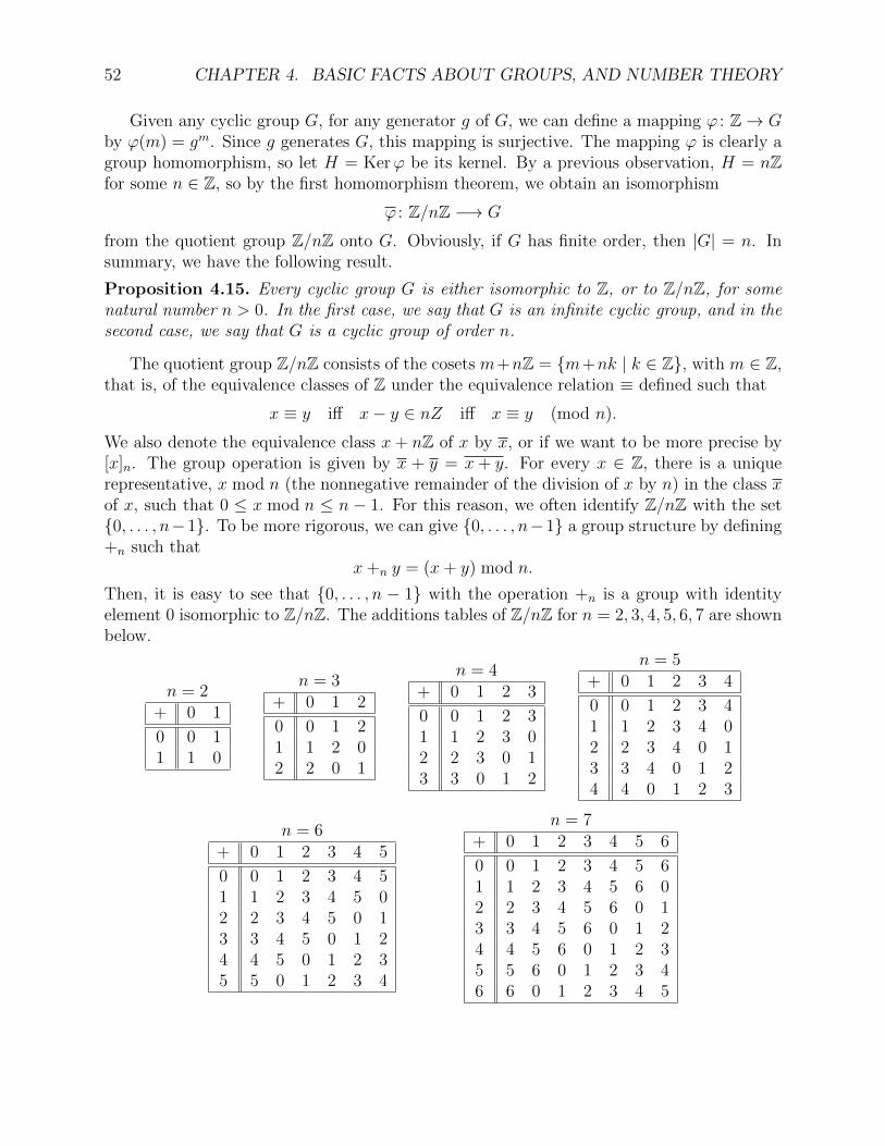
52 CHAPTER 4. BASIC FACTS ABOUT GROUPS, AND NUMBER THEORY
Given any cyclic group G, for any generator g of G, we can define a mapping ϕ : Z→ Gby ϕ(m) = gm. Since g generates G, this mapping is surjective. The mapping ϕ is clearly agroup homomorphism, so let H = Kerϕ be its kernel. By a previous observation, H = nZfor some n ∈ Z, so by the first homomorphism theorem, we obtain an isomorphism
ϕ : Z/nZ −→ G
from the quotient group Z/nZ onto G. Obviously, if G has finite order, then |G| = n. Insummary, we have the following result.
Proposition 4.15. Every cyclic group G is either isomorphic to Z, or to Z/nZ, for somenatural number n > 0. In the first case, we say that G is an infinite cyclic group, and in thesecond case, we say that G is a cyclic group of order n.
The quotient group Z/nZ consists of the cosets m+nZ = m+nk | k ∈ Z, with m ∈ Z,that is, of the equivalence classes of Z under the equivalence relation ≡ defined such that
x ≡ y iff x− y ∈ nZ iff x ≡ y (mod n).
We also denote the equivalence class x + nZ of x by x, or if we want to be more precise by[x]n. The group operation is given by x + y = x+ y. For every x ∈ Z, there is a uniquerepresentative, x mod n (the nonnegative remainder of the division of x by n) in the class xof x, such that 0 ≤ x mod n ≤ n − 1. For this reason, we often identify Z/nZ with the set0, . . . , n−1. To be more rigorous, we can give 0, . . . , n−1 a group structure by defining+n such that
x+n y = (x+ y) mod n.
Then, it is easy to see that 0, . . . , n − 1 with the operation +n is a group with identityelement 0 isomorphic to Z/nZ. The additions tables of Z/nZ for n = 2, 3, 4, 5, 6, 7 are shownbelow.
n = 2+ 0 1
0 0 11 1 0
n = 3+ 0 1 2
0 0 1 21 1 2 02 2 0 1
n = 4+ 0 1 2 3
0 0 1 2 31 1 2 3 02 2 3 0 13 3 0 1 2
n = 5+ 0 1 2 3 4
0 0 1 2 3 41 1 2 3 4 02 2 3 4 0 13 3 4 0 1 24 4 0 1 2 3
n = 6+ 0 1 2 3 4 5
0 0 1 2 3 4 51 1 2 3 4 5 02 2 3 4 5 0 13 3 4 5 0 1 24 4 5 0 1 2 35 5 0 1 2 3 4
n = 7+ 0 1 2 3 4 5 6
0 0 1 2 3 4 5 61 1 2 3 4 5 6 02 2 3 4 5 6 0 13 3 4 5 6 0 1 24 4 5 6 0 1 2 35 5 6 0 1 2 3 46 6 0 1 2 3 4 5
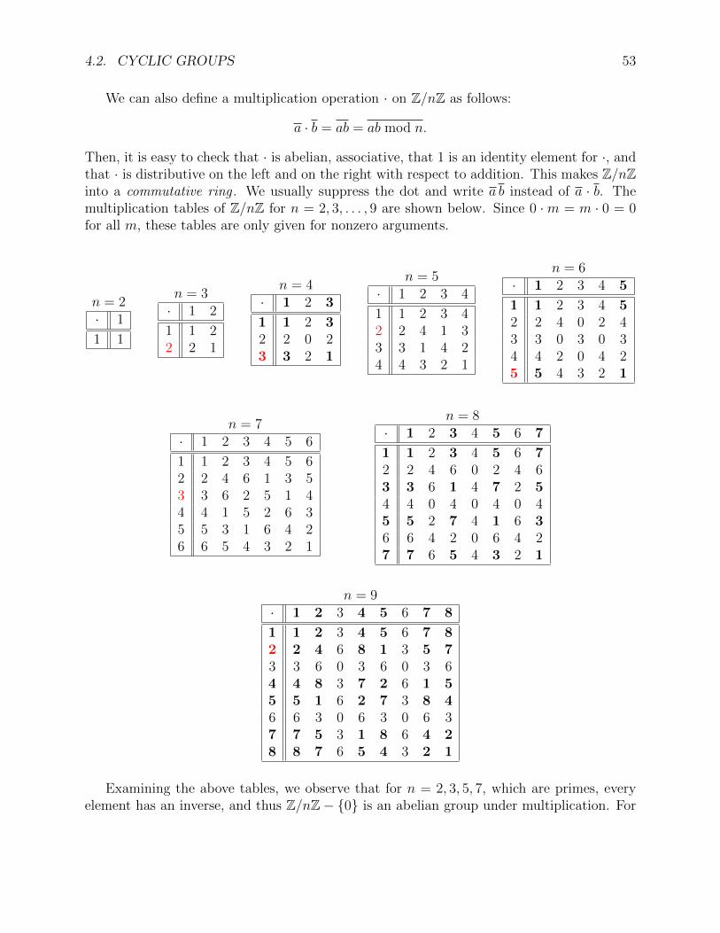
4.2. CYCLIC GROUPS 53
We can also define a multiplication operation · on Z/nZ as follows:
a · b = ab = ab mod n.
Then, it is easy to check that · is abelian, associative, that 1 is an identity element for ·, andthat · is distributive on the left and on the right with respect to addition. This makes Z/nZinto a commutative ring . We usually suppress the dot and write a b instead of a · b. Themultiplication tables of Z/nZ for n = 2, 3, . . . , 9 are shown below. Since 0 ·m = m · 0 = 0for all m, these tables are only given for nonzero arguments.
n = 2· 1
1 1
n = 3· 1 2
1 1 22 2 1
n = 4· 1 2 3
1 1 2 32 2 0 23 3 2 1
n = 5· 1 2 3 4
1 1 2 3 42 2 4 1 33 3 1 4 24 4 3 2 1
n = 6· 1 2 3 4 5
1 1 2 3 4 52 2 4 0 2 43 3 0 3 0 34 4 2 0 4 25 5 4 3 2 1
n = 7· 1 2 3 4 5 6
1 1 2 3 4 5 62 2 4 6 1 3 53 3 6 2 5 1 44 4 1 5 2 6 35 5 3 1 6 4 26 6 5 4 3 2 1
n = 8· 1 2 3 4 5 6 7
1 1 2 3 4 5 6 72 2 4 6 0 2 4 63 3 6 1 4 7 2 54 4 0 4 0 4 0 45 5 2 7 4 1 6 36 6 4 2 0 6 4 27 7 6 5 4 3 2 1
n = 9· 1 2 3 4 5 6 7 8
1 1 2 3 4 5 6 7 82 2 4 6 8 1 3 5 73 3 6 0 3 6 0 3 64 4 8 3 7 2 6 1 55 5 1 6 2 7 3 8 46 6 3 0 6 3 0 6 37 7 5 3 1 8 6 4 28 8 7 6 5 4 3 2 1
Examining the above tables, we observe that for n = 2, 3, 5, 7, which are primes, everyelement has an inverse, and thus Z/nZ− 0 is an abelian group under multiplication. For

54 CHAPTER 4. BASIC FACTS ABOUT GROUPS, AND NUMBER THEORY
n = 4, 6, 8, 9, the elements a that have an inverse are precisely those that are relatively primeto the modulus n (that is, gcd(a, n) = 1). The subset of these elements, shown in boldface,forms an abelian group under multiplication.
These observations hold in general.
Proposition 4.16. Given any integer n ≥ 1, for any a ∈ Z, the residue class a ∈ Z/nZ isinvertible with respect to multiplication iff gcd(a, n) = 1.
Proof. If a has inverse b in Z/nZ, then a b = 1, which means that
ab ≡ 1 (mod n),
that is ab = 1 + nk for some k ∈ Z, which is the Bezout identity
ab− nk = 1
and implies that gcd(a, n) = 1. Conversely, if gcd(a, n) = 1, then by Bezout’s identity thereexist u, v ∈ Z such that
au+ nv = 1,
so au = 1− nv, that is,
au ≡ 1 (mod n),
which means that a u = 1, so a is invertible in Z/nZ.
Definition 4.14. The group (under multiplication) of invertible elements of the ring Z/nZis denoted by (Z/nZ)∗. Note that this group is abelian and only defined if n ≥ 2.
The Euler ϕ-function plays an important role in the theory of the groups (Z/nZ)∗.
Definition 4.15. Given any positive integer n ≥ 1, the Euler ϕ-function (or Euler totientfunction) is defined such that ϕ(n) is the number of integers a, with 1 ≤ a ≤ n, which arerelatively prime to n; that is, with gcd(a, n) = 1.1
Then, by Proposition 4.16, we see that the group (Z/nZ)∗ has order ϕ(n).
For n = 2, (Z/2Z)∗ = 1, the trivial group. For n = 3, (Z/3Z)∗ = 1, 2, and forn = 4, we have (Z/4Z)∗ = 1, 3. Both groups are isomorphic to the group −1, 1. Forn = 6 = 2 · 3, we have ϕ(6) = 2, which is confirmed since (Z/6Z)∗ = 1, 5, for n = 8, wehave ϕ(8) = 4, which is confirmed since (Z/8Z)∗ = 1, 3, 5, 7, and for n = 9 = 3 ·3, we haveϕ(9) = 6, which is confirmed since (Z/9Z)∗ = 1, 2, 4, 5, 7, 8.
Since gcd(a, n) = 1 for every a ∈ 1, . . . , n− 1 iff n is prime, by Proposition 4.16 we seethat (Z/nZ)∗ = Z/nZ− 0 iff n is prime.
1We allow a = n to accomodate the special case n = 1.
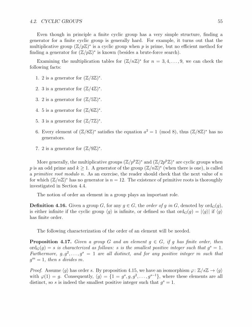
4.2. CYCLIC GROUPS 55
Even though in principle a finite cyclic group has a very simple structure, finding agenerator for a finite cyclic group is generally hard. For example, it turns out that themultiplicative group (Z/pZ)∗ is a cyclic group when p is prime, but no efficient method forfinding a generator for (Z/pZ)∗ is known (besides a brute-force search).
Examining the multiplication tables for (Z/nZ)∗ for n = 3, 4, . . . , 9, we can check thefollowing facts:
1. 2 is a generator for (Z/3Z)∗.
2. 3 is a generator for (Z/4Z)∗.
3. 2 is a generator for (Z/5Z)∗.
4. 5 is a generator for (Z/6Z)∗.
5. 3 is a generator for (Z/7Z)∗.
6. Every element of (Z/8Z)∗ satisfies the equation a2 = 1 (mod 8), thus (Z/8Z)∗ has nogenerators.
7. 2 is a generator for (Z/9Z)∗.
More generally, the multiplicative groups (Z/pkZ)∗ and (Z/2pkZ)∗ are cyclic groups whenp is an odd prime and k ≥ 1. A generator of the group (Z/nZ)∗ (when there is one), is calleda primitive root modulo n. As an exercise, the reader should check that the next value of nfor which (Z/nZ)∗ has no generator is n = 12. The existence of primitive roots is thoroughlyinvestigated in Section 4.4.
The notion of order an element in a group plays an important role.
Definition 4.16. Given a group G, for any g ∈ G, the order of g in G, denoted by ordG(g),is either infinite if the cyclic group 〈g〉 is infinite, or defined so that ordG(g) = |〈g〉| if 〈g〉has finite order.
The following characterization of the order of an element will be needed.
Proposition 4.17. Given a group G and an element g ∈ G, if g has finite order, thenordG(g) = s is characterized as follows: s is the smallest positive integer such that gs = 1.Furthermore, g, g2, . . . , gs = 1 are all distinct, and for any positive integer m such thatgm = 1, then s divides m.
Proof. Assume 〈g〉 has order s. By proposition 4.15, we have an isomorphism ϕ : Z/sZ→ 〈g〉with ϕ(1) = g. Consequently, 〈g〉 = 1 = gs, g, g2, . . . , gs−1, where these elements are alldistinct, so s is indeed the smallest positive integer such that gs = 1.
56 CHAPTER 4. BASIC FACTS ABOUT GROUPS, AND NUMBER THEORY
Conversely, if s is the least positive integer such that gs = 1, then g, g2, . . . , gs = 1 are alldistinct, since otherwise we would have gi = gj for some i, j with 1 ≤ i < j ≤ s, and thenwe would have
gj−i = 1
with 0 < j − i < s, contradicting the minimality of s.
For any n ∈ N, we can write n = sq + r, with 0 ≤ r < s, and we get
gn = gsq+r = (gs)q · gr = gr.
Consequently, 〈g〉 = 1, g, . . . , gs−1, and 〈g〉 has order s.
If gm = 1, then writing m = sq + r, with 0 ≤ r < s, we get
1 = gm = gsq+r = (gs)q · gr = gr,
so gr = 1 with 0 ≤ r < s, contradicting the minimality of s, so r = 0 and s divides m.
The next proposition deals with subgroups of cyclic groups.
Proposition 4.18. Let G = 〈g〉 be a finite cyclic group of order n and let H be any subgroupof G.
(a) The group H is cyclic and generated by some element gk, where k ≥ 1 is the leastinteger such that gk ∈ H.
(b) The order d = |H| of H divides n and n = dk.
(c) We have H = a ∈ G | ad = 1, with d from (b).
(d) For every d ≥ 1, the setHd = a ∈ G | ad = 1
is a cyclic subgroup of G of order gcd(n, d).
(e) For every divisor d of n, there is a unique cyclic subgroup H of order d given by
H = a ∈ G | ad = 1.
Proof. If H = 1, then all claims are true with k = n and d = 1. From now on, assumethat |H| > 1, and pick gk ∈ H with k ≥ 1 minimal. Since |H| > 1, we must have k < n.
(a) For any element gm ∈ H, we can write m = kq + r, with 0 ≤ r < k. Then, we have
gm = gkq+r = (gk)q · gr,
and since gm, gk ∈ H, we have gr = (gk)−q · gm ∈ H. However, 0 ≤ r < k, contradicting theminimality of k, so r = 0. It follows that H = 〈gk〉 is cyclic.
4.2. CYCLIC GROUPS 57
(b) Let us prove that k divides n. Let s = gcd(k, n). By Bezout’s theorem, we can write
s = ku+ nv
for some u, v ∈ Z. Then, since gn = 1, we have
gs = gku+nv = (gk)u · (gn)v = (gk)u,
which shows that gs ∈ H. Since k is the least positive integer such that gk ∈ H, we musthave s = k; that is, k divides n. But then, gk must have order d = n/k, since the order ofgk is the smallest natural number h such that gkh = 1, and since n = dk is the order of g, itmust divide hk, which means that d must divide h, and so h = d.
(c) From (b), H = gk, g2k, . . . , gdk = 1, and we have (gjk)d = (gdk)j = 1, which showsthat every a ∈ H satisfies the equation ad = 1. Conversely, if a ∈ H satisfies ad = 1, sincea = gi for some i, we have gid = 1, and since g has order n, the number n = kd must divideid, which means that k must divide i. Consequently, a = (gk)i/k ∈ H.
(d) It is immediately verified that Hd is a subgroup of G. We have a = gi ∈ Hd iff(gi)d = gid = 1. Write r = gcd(d, n), n = n1r and d = d1r. Then gcd(n1, d1) = 1. Since ghas order n, the number n = n1r divides id = id1r, so n1 divides id1. Since gcd(n1, d1) = 1,the number n1 divides i, and since 1 ≤ i ≤ n, we conclude that i = n1, 2n1, . . . , rn1 = n.Therefore, Hd has order r = gcd(d, n).
(e) This follows immediately from (d).
Proposition 4.19. Let G = 〈g〉 be a finite cyclic group of order n. Then we have:
(a) For any a ∈ G, the order ordG(a) of a divides n.
(b) For any i, with 1 ≤ i ≤ n, the order of gi is n/gcd(i, n).
(c) For every divisor d of n, the group G contains ϕ(d) elements of order d. In particular,a cyclic group of order n has ϕ(n) generators.
Proof. (a) The order ordG(a) of a is the order of the cyclic group 〈a〉, and by Lagrange’stheorem (Proposition 4.7), ordG(a) divides n.
(b) Write k = gcd(i, n), i = i1k, and n = n1k. The order d of gi is the smallest positiveinteger such that (gi)d = gid = 1. Since g has order n, the number n = n1k must divideid = i1kd, so that n1 divides i1d. Since gcd(i1, n1) = 1, the number n1 must divide d, andso d = n1 = n/k, as claimed.
(c) By (b), we need to know how many i ∈ 1, . . . , n have the property n/gcd(i, n) = d,or equivalently
gcd(i, n) = n/d = k.
Obviously, i must be of the form i = jk, with 1 ≤ j ≤ d. Now,
k = gcd(i, n) = gcd(jk, dk) = k gcd(j, d),

58 CHAPTER 4. BASIC FACTS ABOUT GROUPS, AND NUMBER THEORY
so gcd(j, d) = 1. But, there are ϕ(d) integers i ∈ 1, . . . , d such that gcd(j, d) = 1, whichyields (c).
Here is another useful proposition.
Proposition 4.20. For any abelian group G, if a is an element of finite order n1, b is anelement of finite order n2, and gcd(n1, n2) = 1, then a+ b has order n1n2.
Proof. The first step is to prove that 〈a〉 ∩ 〈b〉 = 0. This is because 〈a〉 ∩ 〈b〉 is a subgroupof both 〈a〉 and 〈b〉, so by Lagrange’s theorem, the order m of 〈a〉 ∩ 〈b〉 divide both n1 andn2. Since gcd(n1, n2) = 1, we must have m = 1. Next, we claim that if k(a + b) = 0, thenka = kb = 0. This is because if k(a + b) = 0, then ka = −kb, so ka, kb ∈ 〈a〉 ∩ 〈b〉 = 0,which means that ka = 0 and kb = 0. Now, the order of a+ b is the smallest positive integers such that s(a + b) = 0. From what we just proved, sa = 0 and sb = 0, and since n1 andn2 are the orders of a and b respectively, n1 and n2 must divide s. Since gcd(n1, n2) = 1, weconclude that n1n2 divides s. On the other hand, since n1 and n2 are the orders of a and brespectively, n1a = 0 and n2b = 0, so n1n2(a + b) = n2n1a + n1n2b = 0, and since s is theleast positive integer such that s(a + b) = 0, we see that s divides n1n2, so we must haves = n1n2.
We can now prove the following important fact.
Proposition 4.21. For every integer n ≥ 1, we have
n =∑d|n
ϕ(d).
Proof. By Proposition 4.18 (e), for every divisor d of n, there is a unique cyclic subgroupCd of Z/nZ of order d, and let Φd be the set of generators of Cd. Clearly, the sets Φd arepairwise disjoint. Every g ∈ Z/nZ generates a cyclic group 〈g〉 of some order d, which byProposition 4.18 (b) and (e) must be the cyclic subgroup Cd for some divisor d of n, so g is agenerator for Cd, which means that g ∈ Φd. It follows that the subsets Φd form a partition ofZ/nZ, and since by Proposition 4.19, each group Cd has ϕ(d) generators, we conclude that
n = |Z/nZ| =∑d|n
|Φd| =∑d|n
ϕ(d),
as claimed.
Proposition 4.21 yields a very useful characterization of cyclic groups. The proof is dueto J.P. Serre; see Serre [20].
Theorem 4.22. Let G be a finite group of order n. Then, G is cyclic iff for every divisord of n, there are at most d elements a ∈ G such that ad = 1.
4.2. CYCLIC GROUPS 59
Proof. If G is cyclic, we proved in Proposition 4.18 that for every divisor d of n there is aunique subgroup of order d given by Hd = a ∈ G | ad = 1.
Let us now prove the converse. If there is some x ∈ G of order d, then the subgroup〈x〉 = x, x2, . . . , xd = 1 is cyclic of order d, and the d elements in 〈x〉 satisfy the equationad = 1. If some y ∈ G satisfies the equation yd = 1, then we already have d solutions in 〈x〉,so y ∈ 〈x〉. In particular, all elements of G of order d are generators of 〈x〉, and there areϕ(d) such elements. Hence, the number of elements of G of order d is either 0 or ϕ(d). If itwere 0 for some divisor d of n, then the formula
n =∑d|n
ϕ(d).
from Proposition 4.21 would say that G has strictly less than n elements, a contradiction.Therefore, for every divisor d of n, there are ϕ(d) elements of order d. In particular, forn = d, we have an element x of order n, which shows that G = 〈x〉 is cyclic.
We also have the following simple result which yields a short proof of a result of Euler.
Proposition 4.23. If G is any finite group of order n, then the order of any element g ∈ Gdivides n. Thus,
gn = 1, for all g ∈ G.
Proof. The cyclic subgroup 〈g〉 is a subgroup of G, so by Lagrange’s theorem, its order kdivides the order of G. By Proposition 4.17, we have gk = 1, and since k divides n we getgn = 1.
For any integer n ≥ 2, let (Z/nZ)∗ be the group of invertible elements of the ring Z/nZ.This is a group of order ϕ(n). Then, Proposition 4.23 yields the following result.
Theorem 4.24. (Euler) For any integer n ≥ 2 and any a ∈ 1, . . . , n − 1 such thatgcd(a, n) = 1, we have
aϕ(n) ≡ 1 (mod n).
In particular, if n is a prime, then ϕ(n) = n− 1, and we get Fermat’s little theorem.
Theorem 4.25. (Fermat’s little theorem) For any prime p and any a ∈ 1, . . . , p− 1, wehave
ap−1 ≡ 1 (mod p).
60 CHAPTER 4. BASIC FACTS ABOUT GROUPS, AND NUMBER THEORY
4.3 Rings and Fields
The groups Z,Q,R, C, Z/nZ, and Mn(R) are more than abelian groups, they are alsocommutative rings. Furthermore, Q, R, and C are fields. We now introduce rings and fields.
Definition 4.17. A ring is a set A equipped with two operations +: A × A → A (calledaddition) and ∗ : A× A→ A (called multiplication) having the following properties:
(R1) A is an abelian group w.r.t. +;
(R2) ∗ is associative and has an identity element 1 ∈ A;
(R3) ∗ is distributive w.r.t. +.
The identity element for addition is denoted 0, and the additive inverse of a ∈ A isdenoted by −a. More explicitly, the axioms of a ring are the following equations which holdfor all a, b, c ∈ A:
a+ (b+ c) = (a+ b) + c (associativity of +) (4.1)
a+ b = b+ a (commutativity of +) (4.2)
a+ 0 = 0 + a = a (zero) (4.3)
a+ (−a) = (−a) + a = 0 (additive inverse) (4.4)
a ∗ (b ∗ c) = (a ∗ b) ∗ c (associativity of ∗) (4.5)
a ∗ 1 = 1 ∗ a = a (identity for ∗) (4.6)
(a+ b) ∗ c = (a ∗ c) + (b ∗ c) (distributivity) (4.7)
a ∗ (b+ c) = (a ∗ b) + (a ∗ c) (distributivity) (4.8)
The ring A is commutative if
a ∗ b = b ∗ a for all a, b ∈ A.
From (4.7) and (4.8), we easily obtain
a ∗ 0 = 0 ∗ a = 0 (4.9)
a ∗ (−b) = (−a) ∗ b = −(a ∗ b). (4.10)
Note that (4.9) implies that if 1 = 0, then a = 0 for all a ∈ A, and thus, A = 0. Thering A = 0 is called the trivial ring . A ring for which 1 6= 0 is called nontrivial . Themultiplication a ∗ b of two elements a, b ∈ A is often denoted by ab.
Example 4.6.
1. The additive groups Z,Q,R,C, are commutative rings.

4.3. RINGS AND FIELDS 61
2. For any positive integer n ∈ N, the group Z/nZ is a group under addition. We canalso define a multiplication operation by
a · b = ab = ab mod n,
for all a, b ∈ Z. The reader will easily check that the ring axioms are satisfied, with 0as zero and 1 as multiplicative unit. The resulting ring is denoted by Z/nZ.2
3. The group R[X] of polynomials in one variable with real coefficients is a ring undermultiplication of polynomials. It is a commutative ring.
4. Let d be any positive integer. If d is not divisible by any integer of the form m2, withm ∈ N and m ≥ 2, then we say that d is square-free. For example, d = 1, 2, 3, 5, 6, 7, 10are square-free, but 4, 8, 9, 12 are not square-free. If d is any square-free integer and ifd ≥ 2, then the set of real numbers
Z[√d] = a+ b
√d ∈ R | a, b ∈ Z
is a commutative a ring. If z = a + b√d ∈ Z[
√d], we write z = a − b
√d. Note that
zz = a2 − db2.
5. Similarly, if d ≥ 1 is a positive square-free integer, then the set of complex numbers
Z[√−d] = a+ ib
√d ∈ C | a, b ∈ Z
is a commutative ring. If z = a + ib√d ∈ Z[
√−d], we write z = a− ib
√d. Note that
zz = a2 + db2. The case where d = 1 is a famous example that was investigated byGauss, and Z[
√−1], also denoted Z[i], is called the ring of Gaussian integers .
6. The group of n× n matrices Mn(R) is a ring under matrix multiplication. However, itis not a commutative ring.
7. The group C(a, b) of continuous functions f : (a, b) → R is a ring under the operationf · g defined such that
(f · g)(x) = f(x)g(x)
for all x ∈ (a, b).
Definition 4.18. Given a ring A, for any element a ∈ A, if there is some element b ∈ Asuch that b 6= 0 and ab = 0, then we say that a is a zero divisor . A ring A is an integraldomain (or an entire ring) if 0 6= 1, A is commutative, and ab = 0 implies that a = 0 orb = 0, for all a, b ∈ A. In other words, an integral domain is a nontrivial commutative ringwith no zero divisors besides 0.
2The notation Zn is sometimes used instead of Z/nZ but it clashes with the notation for the n-adicintegers so we prefer not to use it.

62 CHAPTER 4. BASIC FACTS ABOUT GROUPS, AND NUMBER THEORY
Example 4.7.
1. The rings Z,Q,R,C, are integral domains.
2. The ring R[X] of polynomials in one variable with real coefficients is an integral domain.
3. For any positive integer, n ∈ N, we have the ring Z/nZ. Observe that if n is composite,then this ring has zero-divisors. For example, if n = 4, then we have
2 · 2 ≡ 0 (mod 4).
The reader should prove that Z/nZ is an integral domain iff n is prime (use Proposition4.16).
4. If d is a square-free positive integer and if d ≥ 2, the ring Z[√d] is an integral domain.
Similarly, if d ≥ 1 is a square-free positive integer, the ring Z[√−d] is an integral
domain. Finding the invertible elements of these rings is a very interesting problem.
5. The ring of n× n matrices Mn(R) has zero divisors.
A homomorphism between rings is a mapping preserving addition and multiplication(and 0 and 1).
Definition 4.19. Given two rings A and B, a homomorphism between A and B is a functionh : A→ B satisfying the following conditions for all x, y ∈ A:
h(x+ y) = h(x) + h(y)
h(xy) = h(x)h(y)
h(0) = 0
h(1) = 1.
Actually, because B is a group under addition, h(0) = 0 follows from
h(x+ y) = h(x) + h(y).
Example 4.8.
1. If A is a ring, for any integer n ∈ Z, for any a ∈ A, we define n · a by
n · a = a+ · · ·+ a︸ ︷︷ ︸n
if n ≥ 0 (with 0 · a = 0) andn · a = −(−n) · a
if n < 0. Then, the map h : Z→ A given by
h(n) = n · 1A
is a ring homomorphism (where 1A is the multiplicative identity of A).
4.3. RINGS AND FIELDS 63
2. Given any real λ ∈ R, the evaluation map ηλ : R[X]→ R defined by
ηλ(f(X)) = f(λ)
for every polynomial f(X) ∈ R[X] is a ring homomorphism.
Definition 4.20. A ring homomorphism h : A → B is an isomorphism iff there is a ringhomomorphism g : B → A such that g f = idA and f g = idB. An isomorphism from aring to itself is called an automorphism.
As in the case of a group isomorphism, the homomorphism g is unique and denoted byh−1, and it is easy to show that a bijective ring homomorphism h : A→ B is an isomorphism.
Definition 4.21. Given a ring A, a subset A′ of A is a subring of A if A′ is a subgroup ofA (under addition), is closed under multiplication, and contains 1.
For example, we have the following sequence in which every ring on the left of an inlcusionsign is a subring of the ring on the right of the inclusion sign:
Z ⊆ Q ⊆ R ⊆ C.
The ring Z is a subring of both Z[√d] and Z[
√−d], the ring Z[
√d] is a subring of R and the
ring Z[√−d] is a subring of C.
If h : A→ B is a homomorphism of rings, then it is easy to show for any subring A′, theimage h(A′) is a subring of B, and for any subring B′ of B, the inverse image h−1(B′) is asubring of A.
As for groups, the kernel of a ring homomorphism h : A→ B is defined by
Ker h = a ∈ A | h(a) = 0.
Just as in the case of groups, we have the following criterion for the injectivity of a ringhomomorphism. The proof is identical to the proof for groups.
Proposition 4.26. If h : A → B is a homomorphism of rings, then h : A → B is injectiveiff Ker h = 0. (We also write Ker h = (0).)
The kernel of a ring homomorphism is an abelian subgroup of the additive group A, butin general it is not a subring of A, because it may not contain the multiplicative identityelement 1. However, it satisfies the following closure property under multiplication:
ab ∈ Ker h and ba ∈ Ker h for all a ∈ Ker h and all b ∈ A.
This is because if h(a) = 0, then for all b ∈ A we have
h(ab) = h(a)h(b) = 0h(b) = 0 and h(ba) = h(b)h(a) = h(b)0 = 0.
64 CHAPTER 4. BASIC FACTS ABOUT GROUPS, AND NUMBER THEORY
Definition 4.22. Given a ring A, an additive subgroup I of A satisfying the property below
ab ∈ I and ba ∈ I for all a ∈ I and all b ∈ A (∗ideal)
is called a two-sided ideal . If A is a commutative ring, we simply say an ideal .
It turns out that for any ring A and any two-sided ideal I, the set A/I of additive cosetsa + I (with a ∈ A) is a ring called a quotient ring . Then we have the following analog ofProposition 4.11, also called the first isomorphism theorem.
Proposition 4.27. Given a homomorphism of rings h : A → B, the rings A/Ker h andIm h = h(A) are isomorphic.
A field is a commutative ring K for which A− 0 is a group under multiplication.
Definition 4.23. A set K is a field if it is a ring and the following properties hold:
(F1) 0 6= 1;
(F2) K∗ = K − 0 is a group w.r.t. ∗ (i.e., every a 6= 0 has an inverse w.r.t. ∗);
(F3) ∗ is commutative.
If ∗ is not commutative but (F1) and (F2) hold, we say that we have a skew field (ornoncommutative field).
Note that we are assuming that the operation ∗ of a field is commutative. This conventionis not universally adopted, but since ∗ will be commutative for most fields we will encounter,we may as well include this condition in the definition.
Example 4.9.
1. The rings Q, R, and C are fields.
2. The set of (formal) fractions f(X)/g(X) of polynomials f(X), g(X) ∈ R[X], whereg(X) is not the null polynomial, is a field.
3. The ring C(a, b) of continuous functions f : (a, b) → R such that f(x) 6= 0 for allx ∈ (a, b) is a field.
4. Using Proposition 4.16, it is easy to see that the ring Z/pZ is a field iff p is prime.
5. If d is a square-free positive integer and if d ≥ 2, the set
Q(√d) = a+ b
√d ∈ R | a, b ∈ Q
is a field. If z = a + b√d ∈ Q(
√d) and z = a − b
√d, then it is easy to check that if
z 6= 0, then z−1 = z/(zz).

4.3. RINGS AND FIELDS 65
6. Similarly, If d ≥ 1 is a square-free positive integer, the set of complex numbers
Q(√−d) = a+ ib
√d ∈ C | a, b ∈ Q
is a field. If z = a + ib√d ∈ Q(
√−d) and z = a− ib
√d, then it is easy to check that
if z 6= 0, then z−1 = z/(zz).
Definition 4.24. A homomorphism h : K1 → K2 between two fields K1 and K2 is just ahomomorphism between the rings K1 and K2.
However, because K∗1 and K∗2 are groups under multiplication, a homomorphism of fieldsmust be injective.
Proof. First, observe that for any x 6= 0,
1 = h(1) = h(xx−1) = h(x)h(x−1)
and1 = h(1) = h(x−1x) = h(x−1)h(x),
so h(x) 6= 0 andh(x−1) = h(x)−1.
But then, if h(x) = 0, we must have x = 0. Consequently, h is injective.
Definition 4.25. A field homomorphism h : K1 → K2 is an isomorphism iff there is ahomomorphism g : K2 → K1 such that g f = idK1 and f g = idK2 . An isomorphism froma field to itself is called an automorphism.
Then, just as in the case of rings, g is unique and denoted by h−1, and a bijective fieldhomomorphism h : K1 → K2 is an isomorphism.
Definition 4.26. Since every homomorphism h : K1 → K2 between two fields is injective,the image f(K1) of K1 is a subfield of K2. We say that K2 is an extension of K1.
For example, R is an extension of Q and C is an extension of R. The fields Q(√d) and
Q(√−d) are extensions of Q, the field R is an extension of Q(
√d) and the field C is an
extension of Q(√−d).
Definition 4.27. A field K is said to be algebraically closed if every polynomial p(X) withcoefficients in K has some root in K; that is, there is some a ∈ K such that p(a) = 0.
It can be shown that every field K has some minimal extension Ω which is algebraicallyclosed, called an algebraic closure of K. For example, C is the algebraic closure of R. Thealgebraic closure of Q is called the field of algebraic numbers . This field consists of allcomplex numbers that are zeros of a polynomial with coefficients in Q.

66 CHAPTER 4. BASIC FACTS ABOUT GROUPS, AND NUMBER THEORY
Definition 4.28. Given a field K and an automorphism h : K → K of K, it is easy to checkthat the set
Fix(h) = a ∈ K | h(a) = a
of elements of K fixed by h is a subfield of K called the field fixed by h.
For example, if d ≥ 2 is square-free, then the map c : Q(√d)→ Q(
√d) given by
c(a+ b√d) = a− b
√d
is an automorphism of Q(√d), and Fix(c) = Q.
If K is a field, we have the ring homomorphism h : Z → K given by h(n) = n · 1. If his injective, then K contains a copy of Z, and since it is a field, it contains a copy of Q. Inthis case, we say that K has characteristic 0. If h is not injective, then h(Z) is a subring ofK, and thus an integral domain, the kernel of h is a subgroup of Z, which by Proposition4.14 must be of the form pZ for some p ≥ 1. By the first isomorphism theorem, h(Z) isisomorphic to Z/pZ for some p ≥ 1. But then, p must be prime since Z/pZ is an integraldomain iff it is a field iff p is prime. The prime p is called the characteristic of K, and wealso says that K is of finite characteristic.
Definition 4.29. If K is a field, then either
(1) n · 1 6= 0 for all integer n ≥ 1, in which case we say that K has characteristic 0, or
(2) There is some smallest prime number p such that p · 1 = 0 called the characteristic ofK, and we say K is of finite characteristic.
A field K of characteristic 0 contains a copy of Q, thus is infinite. As we will see inSection 4.7, a finite field has nonzero characteristic p. However, there are infinite fields ofnonzero characteristic.
If K2 is a field extension of K1, then K2 is a vector space over K1.
Definition 4.30. If K2 is a field extension of K1 and if the K1-vector space K2 has finitedimension m, we say that K2 is an extension of degree m over K1. The degree of K2 overK1 is denoted by [K2 : K1].
For example, the fields Q(√d) and Q(
√−d) have degree 2 over Q.
Finite fields can be completely classified, which is the object Section 4.7.

4.4. PRIMITIVE ROOTS 67
4.4 Primitive Roots
In this section, we prove that certain multiplicative groups of the form (Z/nZ)∗ are cyclic. Itturns out that the group (Z/nZ)∗ is cyclic if n = 2, 4, pm, and 2pm, where p is an odd primeand m ≥ 1. A generator for (Z/nZ)∗ is called a primitive root modulo n. This terminologygoes back to Euler, and is also used by Gauss in his Disquisitiones Arithmeticae [7]; seeArticle 57. In fact, it is remarkable that most of the results of this section are due to Gauss.Translations of the Disquisitiones Arithmeticae are available, for example, in French, and wehighly recommend reading Articles 52 through 93. Gauss’ style is strikingly lively and clear.Basically all the results of this section are also proved in another famous book, namely theVorlesungen uber Zahlentheorie, by Lejeune–Dirichlet [12]. This book was actually writtenby Richard Dedekind and published in 1863 after Dirichlet’s death in 1859. The Englishtranslation is by John Stillwell. We were amazed to see that most contemporary books onnumber theory, including Apostol excellent’s book [1], give proofs of the existence of primitiveroots, and proofs of the quadratic reciprocity theorem, which are basically Dirichlet’s proofs.
First, we review a basic structure theorem for the rings of the form Z/nZ. For this, weneed the following form of the Chinese remainder theorem.
Theorem 4.28. (Chinese remainder theorem, abstract version) For any integer n ≥ 1, ifn = n1 · · ·nr where the ni are relatively prime in pair, which means that gcd(ni, nj) = 1 forall i 6= j, then we have an isomorphism
Z/nZ ∼= Z/n1Z× · · · × Z/nrZ.
Proof. Consider the map ϕ : Z/nZ→ Z/n1Z× · · · × Z/nrZ given by
ϕ(a) = (a mod n1, . . . , a mod nr).
The map ϕ is a homomorphism, so let’s determine its kernel Kerϕ. We have ϕ(a) = (0, . . . , 0)iff
a ≡ 0 (mod ni), i = 1, . . . , nr,
and since the ni are pairwise relatively prime, this is equivalent to
a ≡ 0 (mod n1 · · ·nr).
Thus, Kerϕ = nZ, and we get an injection
ϕ : Z/nZ −→ Z/n1Z× · · · × Z/nrZ.
However, |Z/nZ| = n = n1 · · ·nr and |Z/n1Z × · · · × Z/nrZ| = n1 · · ·nr, which shows thatϕ is a bijection, and thus an isomorphism.
68 CHAPTER 4. BASIC FACTS ABOUT GROUPS, AND NUMBER THEORY
Theorem 4.28 does not explicitly tells us how to solve a system of congruences
x ≡ b1 (mod n1)
...
x ≡ br (mod nr),
but the following version of the Chinese remainder theorem tells us how to do so.
Theorem 4.29. (Chinese remainder theorem) For any integer n ≥ 1, if n = n1 · · ·nr wherethe ni are relatively prime in pair, which means that gcd(ni, nj) = 1 for all i 6= j, for anyb1, . . . , br ∈ Z, there exists a unique x with 0 ≤ x ≤ n− 1 such that
x ≡ b1 (mod n1)
...
x ≡ br (mod nr).
Proof. Let mi = n/ni, for i = 1, . . . , r. Since the ni are pairwise relatively prime, we havegcd(mi, ni) = 1, so mi has a unique inverse m′i modulo ni; that is,
mim′i ≡ 1 (mod ni).
Letx = b1m1m
′1 + · · ·+ brmrm
′r.
We claim that x is a solution of our congruences. Indeed, since each mj contains the factorni if i 6= j, we have
b1m1m′1 + · · ·+ brmrm
′r ≡ bimim
′i (mod ni),
and since mim′i ≡ 1 (mod ni), we get
b1m1m′1 + · · ·+ brmrm
′r ≡ bi (mod ni),
as required. The uniqueness of x follows from Theorem 4.28. We can also observe that if x, yare two solutions such that 0 ≤ x, y ≤ n − 1, then x ≡ y (mod ni) for i = 1, . . . , r, whichimplies x ≡ y (mod n), and thus x = y.
Interestingly, Theorem 4.28 also applies to the group (Z/nZ)∗ of units (invertible ele-ments) of the ring Z/nZ. Note that we must have n ≥ 2.
Theorem 4.30. For any integer n > 1, if n = n1 · · ·nr where the ni are relatively prime inpair, which means that gcd(ni, nj) = 1 for all i 6= j, then we have an isomorphism
(Z/nZ)∗ ∼= (Z/n1Z)∗ × · · · × (Z/nrZ)∗.

4.4. PRIMITIVE ROOTS 69
Proof. By Theorem 4.28, we have an isomorphism
Z/nZ ∼= Z/n1Z× · · · × Z/nrZ.
However, an element (a1, . . . , ar) of the product ring Z/n1Z × · · · × Z/nrZ is invertible iffeach ai is invertible in Z/niZ, which shows that the above isomorphism induces a groupisomorphism
(Z/nZ)∗ ∼= (Z/n1Z)∗ × · · · × (Z/nrZ)∗,
as claimed.
As a corollary of Theorem 4.30, since the group (Z/niZ)∗ has order ϕ(ni), we obtain themultiplicative property of the Euler ϕ-function.
Proposition 4.31. For any two positive integers m,n, if gcd(m,n) = 1, then
ϕ(mn) = ϕ(m)ϕ(n).
If p is prime then ϕ(p) = p − 1. Also, if k ≥ 2 and if p is prime, then the numbersbetween 1 and pk not relatively prime to pk are of the form ps with 1 ≤ s ≤ pk−1 soϕ(pk) = pk−pk−1 = pk−1(p−1). Since these equations are used a lot, we record them below.
For every prime number p, for all m ≥ 2, we have
ϕ(p) = p− 1, ϕ(pm) = pm−1(p− 1). (∗ϕ)
Using Proposition 4.31 and the above equations, we can compute ϕ(n) for every n (westart with ϕ(1) = 1). Since every positive integer n > 1 has a unique prime factorization
n = pk11 · · · pkrr ,
we get
ϕ(n) = pk1−11 · · · pkr−1r (p1 − 1) · · · (pr − 1) = n
(1− 1
p1
)· · ·(
1− 1
pr
).
As an application of Proposition 4.31 and Theorem 4.24, we prove the property mentionedin the Remark after Proposition 2.3. We begin with the following result.
Proposition 4.32. For any positive integer m ≥ 2 and any integer a such that gcd(a,m) =1, for any two positive integers d, e, if ed ≡ 1 (mod ϕ(m)), then aed ≡ a (mod m).
Proof. Since ed ≡ 1 (mod ϕ(m)) and e, d,m > 0, we can write ed = 1 + kϕ(m) for someinteger k ≥ 0. Since gcd(a,m) = 1, by Euler’s theorem (Theorem 4.24)
aϕ(m) ≡ 1 (mod m),
so we haveaed ≡ a1+kϕ(m) ≡ aakϕ(m) ≡ a(aϕ(m))k ≡ a 1k ≡ a (mod m),
as claimed.
70 CHAPTER 4. BASIC FACTS ABOUT GROUPS, AND NUMBER THEORY
Recall that an integer m is square-free if it is not divisible by any integer d2 with d ≥2. Using Proposition 4.32, we can prove the following result from Niven, Zuckerman, andMontgomery [16] (Section 2.5, Problem 4).
Proposition 4.33. Let m ≥ 2 be any positive square-free integer. For any two positiveintegers d, e, if ed ≡ 1 (mod ϕ(m)), then aed ≡ a (mod m) for all integers a ∈ Z.
Proof. First observe that if g and m are positive integers such that g divides m, then ϕ(g)
divides ϕ(m). This is because we can write g = pi11 · · · pihh and m = pj11 · · · p
jhh p
jh+1
h+1 · · · pjkk , for
some distinct primes p1, . . . , ph, ph+1, . . . , pk, with h ≤ k, 1 ≤ i1 ≤ j1, . . . , 1 ≤ ih ≤ jh, andjh+1, . . . , jk ≥ 1, and we have
ϕ(g) = pi1−11 · · · pih−1h (p1 − 1) · · · (ph − 1)
ϕ(m) = pj1−11 · · · pjh−1h pjh+1−1h+1 · · · pjk−1k (p1 − 1) · · · (ph − 1)(ph+1 − 1) · · · (pk − 1),
so ϕ(g) divides ϕ(m).
If a = 0, then result is trivial, so assume that a 6= 0. Let g = gcd(a,m) and writem = gm1. Since m is square-free, m can be expressed as m = p1 · · · pk for distinct primes pi,and sincem = gm1, the numbers g andm1 have no prime factor in common so gcd(m1, g) = 1.Since g = gcd(a,m), we also have gcd(a,m1) = 1.
By hypothesis ed ≡ 1 (mod ϕ(m)), and since both g and m1 divide m, by the previousobservation ϕ(g) divides ϕ(m) and ϕ(m1) divides ϕ(m). Therefore
ed ≡ 1 (mod ϕ(g)) and ed ≡ 1 (mod ϕ(m1)).
Since gcd(a,m1) = 1, by proposition 4.32 applied to a and m1, we get
aed ≡ a (mod m1). (∗1)
Since g divides a, trivially we have
aed ≡ a (mod g). (∗2)
Since gcd(m1, g) = 1, by the Chinese reminder theorem applied to (∗1) and (∗2), we deducethat
aed ≡ a (mod m),
as claimed.
Observe that if m = pq where p and q are two distinct primes, then Proposition 2.3 is aconsequence of Proposition 4.33. We now return to the existence of primitive roots.
Theorem 4.30 reduces the study of the group (Z/nZ)∗ to the stucture of the groups(Z/pkZ)∗, where p is a prime and k ≥ 1. The case p = 2 is exceptional, but the case wherep is an odd prime is nice; namely, (Z/pkZ)∗ is a cyclic group. We begin with the case k = 1.
4.4. PRIMITIVE ROOTS 71
Theorem 4.34. (Gauss) For every odd prime p, the group (Z/pZ)∗ is cyclic of order p− 1.It has ϕ(p− 1) generators.
Proof. We use Theorem 4.22 applied to G = (Z/pZ)∗ and n = ϕ(p) = p−1. Since p is prime,Z/pZ is a field, for every divisor d of p − 1, the equation xd − 1 = 0 has at most d rootsin Z/pZ, and a fortiori in (Z/pZ)∗. Here, we used the fact known from algebra that everynonzero polynomial of degree d with coefficients in a field has a most d roots. Therefore,(Z/pZ)∗ is cyclic and has ϕ(p− 1) generators.
Definition 4.31. For any positive integer n, the integers a ∈ Z such that a mod n is agenerator of (Z/nZ)∗ are called primitive roots mod n.
Remark: Gauss’ proof is not all that different from the one we gave. For every divisord of p − 1, Gauss defines ψ(d) as the number of integers a, with 1 ≤ a ≤ p − 1, thathave order d, and then proves that ψ(d) = ϕ(d). For this, he proves Proposition 4.21; seeArticles 52–56 of the Disquisitiones Arithmeticae [7]. Gauss also warns about the danger ofregarding as established, statements which are not proved. He goes on to say that “nobodyhas attempted to prove Theorem 4.34, except Euler,” and that Euler has talked extensivelyabout the necessity of proving it, but that his proof is flawed in two respects! A version ofthe same proof is also given in Dirichlet–Dedekind [12] (Chapter 2, Section 30).
Ribenboim reports that Gauss proposes an algorithm for finding a primitive root modulop in Articles 73 and 74 in the Disquisitiones Arithmeticae [7]; see Ribenboim[18] (Chapter2, Section II). The algorithm is as follows:
Step 1. Pick any integer a with 2 ≤ a ≤ p− 1, and find the order t of a, that is, the leastpositive integer such that at ≡ 1 (mod p). If a has order p − 1, then it is a primitive rootmodulo p. Otherwise, go to the next step.
Step 2. Find any any number b, with 2 ≤ b ≤ p − 1, such that b 6≡ ai (mod p), fori = 1, . . . , t. Let u be the order of b, the least positive integer such that bu ≡ 1 (mod p). Iclaim that u does not divide t.
This is because if u divides t, since bu ≡ 1 (mod p), we would get bt ≡ 1 (mod p), butsince the congruence X t ≡ 1 (mod p) has t solutions (a, a2, . . . , at), then we would haveb ≡ ai (mod p) for some i with 1 ≤ i ≤ t, a contradiction. If u = p− 1, then b is a primitiveroot. Otherwise, let y be the least common multiple of t and u. Then, we can split y asy = mn, where gcd(m,n) = 1, m divides t, and n divides u. As explained by Gauss in afootnote, m and n can be obtained from prime factorizations of t and u. All prime powersonly in t are included in m, all prime powers only in u are included in n, and prime powersboth in t and u are included in m or n, it doesn’t matter. Then, a′ ≡ at/m (mod p) hasorder m, b′ ≡ bu/n (mod p) has order n, and because gcd(m,n) = 1, the element c = a′b′ hasorder y = mn > t modulo p. If mn = p− 1, then c is a primitive root modulo p. Otherwise,go back to Step 2 with a = c and t = y.

72 CHAPTER 4. BASIC FACTS ABOUT GROUPS, AND NUMBER THEORY
Since y > t in Step 2, the order of t keeps increasing while dividing p− 1, so eventuallyt = p− 1, and a primitive root is found. Gauss illutrates this process for p = 73, and findsthe primitive root 5. Gauss’ algorithm requires factoring y as mn with gcd(m,n) = 1, andthis step requires prime factorizations of t and u. For large p, this is not a practical method.Still, it is impressive that Gauss gave an algorithm for finding a primitive root over 200 yearsago.
The above algorithm does not necessarily yield the smallest primitive root gp modulo p.It is known that gp > C log p for infinitely many primes (for some constant C), and thatgp < p0.499 for all p > ee
24(see Ribenboim [18], Chapter 2, Section II).
We now consider the case where n = pm, with p prime and m ≥ 2. We follow the beautifulexposition given in Apostol [1]. As we mentioned earlier, this exposition is extremely close toDirichlet’s presentation (as written up by Dedekind) [12]. The following technical propositionis needed.
Proposition 4.35. For any odd prime p, let g be a primitive root modulo p such that
gp−1 6≡ 1 (mod p2).
Then, for all i ≥ 2, we havegϕ(p
i−1) 6≡ 1 (mod pi).
Proof. We proceed by induction on i. The base case i = 2 is the hypothesis since ϕ(p) = p−1as p is prime. For the induction step, assume that
gϕ(pi−1) 6≡ 1 (mod pi). (∗)
By Euler’s theorem,gϕ(p
i−1) ≡ 1 (mod pi−1),
so we havegϕ(p
i−1) = 1 + kpi−1
for some k ∈ Z, and p does not divide k because of (∗). Raising the above equation to thepth power, since ϕ(pi−1) = pi−1 − pi−2 by (∗ϕ), we get pϕ(pi−1) = pi − pi−1 = ϕ(pi), andusing the binomial formula
gϕ(pi) = (1 + kpi−1)p = 1 + kpi + k2
p(p− 1)
2p2(i−1) + rp3(i−1)
= 1 + kpi + k2p− 1
2p2i−1 + rp3(i−1),
for some r ∈ Z. Now, 2i− 1 ≥ i+ 1 and 3i− 3 ≥ i+ 1 since i ≥ 2, so we get the congruence
gϕ(pi) = 1 + kpi (mod pi+1),
where p does not divide k, and therefore
gϕ(pi) 6≡ 1 (mod pi+1),
establishing the induction step.
4.4. PRIMITIVE ROOTS 73
The next step if to “promote” a primitive root modulo p to a primitive root modulo pm.For this, we use the following proposition.
Proposition 4.36. For any odd prime p, there is a primitive root g modulo p such that
gp−1 6≡ 1 (mod p2). (∗)
Proof. Let g be any primitive root modulo p. If (∗) holds, we are done. Otherwise, gp−1 ≡ 1(mod p2), in which case we consider g1 = g + p. Since g is a primitive root modulo p andsince g+ p ≡ g (mod p), the integer g1 is also a primitive root modulo p, and we claim thatit satisfies (∗). By the binomial formula we have
gp−11 = (g + p)p−1
= gp−1 + (p− 1)gp−2p+ tp2,
= gp−1 − gp−2p+ (t+ gp−2)p2,
for some t ∈ Z, and because gp−1 ≡ 1 (mod p2), we get
gp−11 ≡ gp−1 − pgp−2 (mod p2)
≡ 1− pgp−2 (mod p2).
But, we cannot have pgp−2 ≡ 0 (mod p2), for this would imply that gp−2 ≡ 0 (mod p),contradicting the fact that g is a primitive root modulo p. Therefore, gp−11 6≡ 1 (mod p2), asclaimed.
Finally, we can prove that primitive roots modulo pm exist.
Proposition 4.37. For any odd prime p, a primitive root g modulo p is a primitive rootmodulo pm for all m ≥ 2 iff
gp−1 6≡ 1 (mod p2). (∗)
Proof. Suppose that g is a primitive root modulo pm for all m ≥ 1. In particular, g is aprimitive root modulo p2. We have (by Fermat’s little theorem)
gp−1 ≡ 1 (mod p),
and since ϕ(p2) = p(p− 1) > p− 1, if
gp−1 ≡ 1 (mod p2),
then g can’t be a primitive root modulo p2, so gp−1 6≡ 1 (mod p2) must hold.
Conversely, assume that the primitive root g modulo p satisfies (∗). We prove that g isa primitive root modulo pm for all m ≥ 2. Let t be the order of g in (Z/pmZ)∗. We need toprove that
t = ϕ(pm).

74 CHAPTER 4. BASIC FACTS ABOUT GROUPS, AND NUMBER THEORY
Since gt ≡ 1 (mod pm), we also have gt ≡ 1 (mod p), and since g has order p− 1 modulo p,we conclude that p− 1 divides t, so we can write
t = q(p− 1)
for some q ∈ Z. Since g is a primitive root modulo p, we have gcd(g, p) = 1, which impliesgcd(g, pm) = 1, and by Euler’s Theorem we have gϕ(p
m) ≡ 1 (mod pm), and since t is theorder of g modulo pm, the number t must divide ϕ(pm) = pm−1(p − 1); that is, q(p − 1)divides pm−1(p− 1), so q divides pm−1. Therefore, we can write
t = pb(p− 1), with b ≤ m− 1.
If we can prove that b = m− 1, then we are done.
Assume by contradiction that b < m − 1. If so, b ≤ m − 2 and t = pb(p − 1) dividespm−2(p− 1) = ϕ(pm−1). As a consequence, from gt ≡ 1 (mod pm), we get
gϕ(pm−1) ≡ 1 (mod pm).
However, since by assumptiongp−1 6≡ 1 (mod p2),
Proposition 4.35 implies that
gϕ(pi−1) 6≡ 1 (mod pi) for all i ≥ 2,
a contradiction. Therefore, b = m− 1 and the proof is complete.
Putting Propositions 4.36 and 4.37 together, and using the fact that
ϕ(ϕ(pm)) = ϕ(pm−1(p− 1)) = ϕ(pm−1)ϕ(p− 1) = pm−2(p− 1)ϕ(p− 1),
we obtain our theorem.
Theorem 4.38. (Gauss) For every odd prime p and every integer m ≥ 2, the group(Z/pmZ)∗ is cyclic of order pm−1(p−1). Furthermore, it has ϕ(ϕ(pm)) = pm−2(p−1)ϕ(p−1)primitive roots.
Remark: Gauss proves Theorem 4.38 in Articles 82–89 of the Disquisitiones Arithmeticae[7]. The above proof is basically Dedekind’s proof [12] (Supplement V).
The case n = 2pm is easily handled.
Theorem 4.39. For every odd prime p and every integer m ≥ 1, the group (Z/2pmZ)∗
is cyclic. In fact, (Z/2pmZ)∗ ∼= (Z/pmZ)∗. Furthermore, there exist odd primitive roots gmodulo pm, and each such g is also a primitive root modulo 2pm.
4.5. WHICH GROUPS (Z/nZ)∗ HAVE PRIMITIVE ROOTS 75
Proof. Since p is an odd prime, gcd(2, p) = 1, so Theorem 4.30 yields an isomorphism
(Z/2pmZ)∗ ∼= (Z/2Z)∗ × (Z/pmZ)∗ ∼= (Z/pmZ)∗,
since (Z/2Z)∗ is the trivial group 1.If g is a primitive root modulo pm, since g + pm ≡ g (mod pm), the integer g + pm is
also a primitive root modulo pm, and since p is odd, either g or g + pm is odd (pm is odd).Let g be an odd primitive root modulo pm and let t be its order modulo 2pm. We need toprove that t = ϕ(2pm) = ϕ(2)ϕ(pm) = ϕ(pm). Now, t must divide ϕ(2pm) = ϕ(pm), sincegcd(g, pm) = 1 and g odd implies that gcd(g, 2pm) = 1 so by Euler’s theorem gϕ(2p
m) ≡ 1(mod 2pm). On the other hand, gt ≡ 1 (mod 2pm), which implies gt ≡ 1 (mod pm), so ϕ(pm)divides t since g is a primitive root modulo pm (it has order ϕ(pm) modulo pm). Therefore,t = ϕ(pm) = ϕ(2pm), as claimed.
In summary, we proved that primitive roots exist if n = 2, 4, pm, or 2pm where p is anodd prime. In the next section, we show that primitive roots do not exist in all the othercases.
4.5 Which Groups (Z/nZ)∗ Have Primitive Roots
We begin with the case p = 2m with m ≥ 3. Observe that by (∗ϕ), we have ϕ(2m) =2m−1(2− 1) = 2m−1, so if m ≥ 2, then ϕ(2m)/2 = 2m−2.
Proposition 4.40. (Gauss) If a is an odd integer, then for all m ≥ 3, we have
aϕ(2m)/2 ≡ a2
m−2 ≡ 1 (mod 2m).
Therefore, there are no primitive roots modulo 2m.
Proof. We proceed by induction on m. When m = 3, we need to show that a2 ≡ 1 (mod 8),if a is odd. This is because a is of the form a = 2k + 1,
(2k + 1)2 = 4k2 + 4k + 1 = 4k(k + 1) + 1,
and k(k + 1) is always even.
For the induction step, the induction hypothesis says that
a2m−2
= 1 + 2mt,
for some t ∈ Z. Squaring both sides, we get
a2m−1
= 1 + 2m+1t+ 22mt2,
soa2
m−1 ≡ 1 (mod 2m+1),
establishing the induction step.

76 CHAPTER 4. BASIC FACTS ABOUT GROUPS, AND NUMBER THEORY
Remark: Gauss proves Proposition 4.40 in Article 90 of the Disquisitiones Arithmeticae[7]. It also appears in Dirichlet–Dedekind [12] (Supplement V).
In fact, primitive roots do not exist in all the following cases.
Proposition 4.41. Given any integer n ≥ 2, if n is not of the form n = 2, 4, pm, or 2pm,where p is an odd prime, then for any integer a with gcd(a, n) = 1, we have
aϕ(n)/2 ≡ 1 (mod n).
Therefore, there are no primitive roots modulo n.
Proof. We already proved that primitive roots do not exist if n = 2m with m ≥ 3. Therefore,we may assume that n has a factorization of the form
n = 2kpk11 · · · pkss ,
where the pi are odd primes, s ≥ 1, ki ≥ 1, and k ≥ 0. Furthermore, since n is not of theform n = 2, 4, pm, or 2pm, we have k ≥ 2 if s = 1, and s ≥ 2 if k = 0, 1. We have
ϕ(n) = ϕ(2k)ϕ(pk11 ) · · ·ϕ(pkss ).
Pick a ∈ Z such that gcd(a, n) = 1. We need to prove that
aϕ(n)/2 ≡ 1 (mod n).
Let g be a primitive root modulo pk11 , and write
a ≡ gi (mod pk11 ).
Then, we have
aϕ(n)/2 ≡ giϕ(n)/2 ≡ gtϕ(pk11 ) (mod pk11 ),
witht = iϕ(2k)ϕ(pk22 ) · · ·ϕ(pkss )/2.
We claim that t is an integer.
If k ≥ 2, then ϕ(2k) = 2k−1 is even, so t is an integer. If k = 0 or k = 1, then s ≥ 2 andthe factor ϕ(pk22 ) = pk2−12 (p2 − 1) is even, so t is also an integer.
Sincegϕ(p
k11 ) ≡ 1 (mod pk11 ),
fromaϕ(n)/2 ≡ gtϕ(p
k11 ) (mod pk11 ),
we obtainaϕ(n)/2 ≡ 1 (mod pk11 ).
4.5. WHICH GROUPS (Z/nZ)∗ HAVE PRIMITIVE ROOTS 77
A similar proof shows thataϕ(n)/2 ≡ 1 (mod pkii )
for i = 1, . . . s. We still need to prove that a similar congruence holds modulo 2k.
If k ≥ 3, since gcd(a, n) = 1, the number a must be odd, and by Proposition 4.40, wehave
aϕ(2k)/2 ≡ a2
k−2 ≡ 1 (mod 2k).
Since ϕ(2k) divides ϕ(n), we get
aϕ(n)/2 ≡ 1 (mod 2k), k ≥ 3.
If k ≤ 2, then we check directly that
aϕ(2k) ≡ 1 (mod 2k).
If k = 1 or k = 2, since gcd(a, n) = 1, the number a must be odd. If k = 1, sinceϕ(21) = ϕ(2) = 1 and a is odd, we have a ≡ 1 (mod 2) as desired. If k = 2, since a is odd,either a = 4s+ 1 or a = 4s+ 3 for some integer s, but then since ϕ(22) = 2,
a2 ≡ (4s+ 1)2 = 16s2 + 8s+ 1 ≡ 1 (mod 4)
anda2 ≡ (4s+ 3)2 = 16s2 + 24s+ 9 ≡ 1 (mod 4),
as desired.
But if k ≤ 2, then s ≥ 2, so
ϕ(n) = ϕ(2k)ϕ(pk11 ) · · ·ϕ(pkss ) = ϕ(2k)pk1−11 (p1 − 1)ϕ(pk22 ) · · ·ϕ(pkss ) = 2rϕ(2k),
for some integer r. Thus, ϕ(2k) divides ϕ(n)/2, and
aϕ(n)/2 ≡ 1 (mod 2k)
holds for k ≤ 2. In summary, the congruences
aϕ(n)/2 ≡ 1 (mod pkii )
aϕ(n)/2 ≡ 1 (mod 2k)
hold for i = 1, . . . , s and k ≥ 0. Since the moduli are pairwise relatively prime, we obtain
aϕ(n)/2 ≡ 1 (mod n),
as claimed.
Putting everything together, we have the following remarkable result, most of which isdue to Gauss.

78 CHAPTER 4. BASIC FACTS ABOUT GROUPS, AND NUMBER THEORY
Theorem 4.42. The group (Z/nZ)∗ is cyclic of order ϕ(n) iff n = 2, 4, pm, or 2pm, wherep is an odd prime and m ≥ 1. There are ϕ(ϕ(n)) primitive roots modulo n.
Surprisingly, even in the case where n = p is an odd prime, there is no known criterionto determine whether an integer a is a primitive root modulo p. For example, we don’t knowhow to determine if 2 is a primitive root modulo p, other than by computing all powers 2i
modulo p. In fact, we have the following conjecture made by Emil Artin around 1920 (seeSilverman [22], Chapter 21):
Artin’s Conjecture. The number 2 is a primitive root for infinitely many primes.
Also, it is easy to see that a perfect square (a number of the form a2) and −1 are notprimitive roots. Artin also made the following conjecture.
The Generalized Artin Conjecture. Every integer which is not a perfect square andis different from −1 is a primitive root for infinitely many primes.
It has been shown by Christopher Hooley (1967) that if the Extended Riemann Hypoth-esis (ERH) holds, then the generalized Artin conjecture also holds. For a brief decription ofthe ERH, see Section 5.6.
More can be said in the “bad” case n = 2m with m ≥ 3, Amazingly, 5 plays a specialrole.
Proposition 4.43. For any integers x, y, if x ≡ 1 + 4y (mod 8), then
x2k ≡ 1 + 2k+2y (mod 2k+3),
for all k ≥ 0.
Proof. We proceed by induction on k. The case k = 0 is the hypothesis. For the inductionstep, it is enough to prove that if a ≡ 1+2k+1b (mod 2k+2) for some k ≥ 1, then a2 ≡ 1+2k+2b(mod 2k+3).
If a ≡ 1 + 2k+1b (mod 2k+2), then a = 1 + 2k+1b+ c2k+2, for some c, so we get
a2 = (1 + 2k+1b+ c2k+2)2
= (1 + 2k+1(b+ 2c))2
= 1 + 2k+2(b+ 2c) + 22k+2(b+ 2c)2
= 1 + 2k+2b+ 2k+3c+ 22k+2(b+ 2c)2,
and because k ≥ 1, we have 2k + 2 ≥ k + 3, so we get
a2 ≡ 1 + 2k+2b (mod 2k+3),
establishing the induction step.
4.5. WHICH GROUPS (Z/nZ)∗ HAVE PRIMITIVE ROOTS 79
Observe that if we set x = 5 and y = 1, then 5 ≡ 5 (mod 8), so by Proposition 4.43, wehave
52k ≡ 1 + 2k+2 (mod 2k+3), for all k ≥ 0.
On the other hand, since 5 is odd, by Proposition 4.40, we have
52m−2 ≡ 1 (mod 2m).
Therefore, 5 has order 2m−2 modulo 2m. We can use this fact to prove the following result(following Bourbaki [2], Chapter VII, §2.4). This result is more or less implicit in Article91 of the Disquisitiones Arithmeticae [7]. It is explicitly proved in Dirichlet–Dedekind [12](Supplement V).
Theorem 4.44. For any m ≥ 3, the group (Z/2mZ)∗ is isomorphic to the direct product−1, 1 × 〈5〉 of the cyclic subgroup −1, 1 generated by −1 and the cyclic subgroup 〈5〉 oforder 2m−2 generated by 5.
Proof. For m ≥ 3, we have the homomorphism π : (Z/2mZ)∗ → (Z/4Z)∗ given by
π(a mod 2m) = a mod 4.
The kernel of this homomorphism is the subgroup U(2m) of (Z/2mZ)∗ given by
U(2m) = a mod 2m | a ≡ 1 (mod 4),
and so U(2m) has order 2m−2. By the first isomorphism theorem, (Z/4Z)∗ is isomorphicto (Z/2mZ)∗/U(2m), and by Lagrange’s theorem, since (Z/4Z)∗ has order 2 and U(2m) hasorder 2m−2, we conclude that (Z/2mZ)∗ has order 2m−1.
We already know that the cyclic subgroup group 〈5〉 generated by 5 has order 2m−2
modulo 2m, and since 5 ≡ 1 (mod 4), we see that 5 ∈ U(2m), and thus U(2m) = 〈5〉. Weclaim that −1 /∈ 〈5〉. This follows because π(−1) = −1 mod 4, and −1 6≡ 1 (mod 4), so −1does not belong to the kernel U(2m) of π, which is equal to 〈5〉.
I
Consequently, if H = −1, 1 is the subgroup generated by −1, we have H ∩ 〈5〉 = 0.By Proposition 4.12, we have an isomorphism
−1, 1 × 〈5〉 ∼= −1, 1 ⊕ 〈5〉.
Now, (Z/2mZ)∗ has order 2m−1, the subgroup 〈5〉 has order 2m−2, and −1, 1 has order 2,so
(Z/2mZ)∗ = −1, 1 ⊕ 〈5〉
and we have an isomorphism (Z/2mZ)∗ ∼= −1, 1 × 〈5〉.
80 CHAPTER 4. BASIC FACTS ABOUT GROUPS, AND NUMBER THEORY
Remarks: Another way to prove Theorem 4.38 is to proceed as follows (following Bourbaki[2], Chapter VII, §2.4). We have the homomorphism π : (Z/pmZ)∗ → (Z/pZ)∗ given by
π(a mod pm) = a mod p.
The kernel of this homomorphism is the subgroup U(pm) of (Z/pmZ)∗ given by
U(pm) = a mod pm | a ≡ 1 (mod p),
and so U(pm) has order pm−1. By the first isomorphism theorem, (Z/pZ)∗ is isomorphic to(Z/pmZ)∗/U(pm), and by Lagrange’s theorem, since (Z/pZ)∗ has order p− 1 and U(pm) hasorder pm−1, we conclude that (Z/pmZ)∗ has order pm−1(p− 1).
Next, we show that p + 1 has order pm−1 in (Z/pmZ)∗, and since p + 1 ≡ 1 (mod p),p + 1 is a generator for U(pm). For this we prove that if p is an odd prime and x ≡ 1 + py(mod p2), then xp
k ≡ 1 + pk+1y (mod pk+2), for all k ≥ 0.
Then, using a primitive root of (Z/pZ)∗, we can find an element y of order p − 1 in(Z/pmZ)∗. By Proposition 4.20, since gcd(pm−1, p − 1) = 1, we conclude that (p + 1)y hasorder pm−1(p− 1) = ϕ(pm), so (p+ 1)y is a primitive root modulo pm.
4.6 The Lucas Theorem, PRIMES is in NP
In this section we discuss an application of the existence of primitive roots in (Z/pZ)∗ wherep is an odd prime, known an the n− 1 test . This test due to E. Lucas determines whether apositive odd integer n is prime or not by examining the prime factors of n− 1 and checkingsome congruences.
The n− 1 test can be described as the construction of a certain kind of tree rooted withn, and it turns out that the number of nodes in this tree is bounded by 2 log2 n, and thatthe number of modular multiplications involved in checking the congruences is bounded by2 log2
2 n.
Recall that when we talk about the complexity of algorithms dealing with numbers,we assume that all inputs (to a Turing machine) are strings representing these numbers,typically in base 2. Since the length of the binary representation of a natural number n ≥ 1is blog2 nc + 1 (or dlog2(n + 1)e, which allows n = 0), the complexity of algorithms dealingwith (nonzero) numbers m,n, etc. is expressed in terms of log2m, log2 n, etc. Recall that forany real number x ∈ R, the floor of x is the greatest integer bxc that is less that or equal tox, and the ceiling of x is the least integer dxe that is greater that or equal to x. If we chooseto represent numbers in base 10, since for any base b we have logb x = lnx/ ln b, we have
log2 x =ln 10
ln 2log10 x.

4.6. THE LUCAS THEOREM, PRIMES IS IN NP 81
Since (ln 10)/(ln 2) ≈ 3.322 ≈ 10/3, we see that the number of decimal digits needed torepresent the integer n in base 10 is approximately 30% of the number of bits needed torepresent n in base 2.
Since the Lucas test yields a tree such that the number of modular multiplications in-volved in checking the congruences is bounded by 2 log2
2 n, it is not hard to show that testingwhether or not a positive integer n is prime, a problem denoted PRIMES, belongs to thecomplexity class NP. This result was shown by V. Pratt [17] (1975), but Peter Freyd toldme that it was “folklore.” Of course, since 2002, thanks to the AKS algorithm, we knowthat PRIMES actually belongs to the class P, but this is a much harder result.
Here is Lehmer’s version of the Lucas result, from 1876.
Theorem 4.45. (Lucas theorem) Let n be a positive integer with n ≥ 2. Then n is primeiff there is some integer a ∈ 1, 2, . . . , n− 1 such that the following two conditions hold:
(1) an−1 ≡ 1 (mod n).
(2) If n > 2, then a(n−1)/q 6≡ 1 (mod n) for all prime divisors q of n− 1.
Proof. First, assume that Conditions (1) and (2) hold. If n = 2, since 2 is prime, we aredone. Thus assume that n ≥ 3, and let r be the order of a. We claim that r = n − 1. Thecondition an−1 ≡ 1 (mod n) implies that r divides n− 1. Suppose that r < n− 1, and let qbe a prime divisor of (n− 1)/r (so q divides n− 1). Since r is the order or a we have ar ≡ 1(mod n), so we get
a(n−1)/q ≡ ar(n−1)/(rq) ≡ (ar)(n−1)/(rq) ≡ 1(n−1)/(rq) ≡ 1 (mod n),
contradicting Condition (2). Therefore, r = n− 1, as claimed.
We now show that n must be prime. Now an−1 ≡ 1 (mod n) implies that a and n arerelatively prime so by Euler’s Theorem (Theorem 4.24),
aϕ(n) ≡ 1 (mod n).
Since the order of a is n− 1, we have n− 1 ≤ ϕ(n). If n ≥ 3 is not prime, then n has someprime divisor p, but n and p are integers in 1, 2, . . . , n that are not relatively prime to n,so by definition of ϕ(n), we have ϕ(n) ≤ n − 2, contradicting the fact that n − 1 ≤ ϕ(n).Therefore, n must be prime.
Conversely, assume that n is prime. If n = 2, then we set a = 1. Otherwise, pick a to beany primitive root modulo p.
Clearly, if n > 2 then we may assume that a ≥ 2. The main difficulty with the n − 1test is not so much guessing the primitive root a, but finding a complete prime factorizationof n − 1. However, as a nondeterministic algorithm, the n − 1 test yields a “proof” that anumber n is indeed prime which can be represented as a tree, and the number of operations
82 CHAPTER 4. BASIC FACTS ABOUT GROUPS, AND NUMBER THEORY
needed to check the required conditions (the congruences) is bounded by c log22 n for some
positive constant c, and this implies that testing primality is in NP.
Before explaining the details of this method, we sharpen slightly Lucas’ theorem to dealonly with odd prime divisors.
Theorem 4.46. Let n be a positive odd integer with n ≥ 3. Then n is prime iff there is someinteger a ∈ 2, . . . , n − 1 (a guess for a primitive root modulo n) such that the followingtwo conditions hold:
(1b) a(n−1)/2 ≡ −1 (mod n).
(2b) If n− 1 is not a power of 2, then a(n−1)/2q 6≡ −1 (mod n) for all odd prime divisors qof n− 1.
Proof. Assume that Conditions (1b) and (2b) of Theorem 4.46 hold. Then we claim thatConditions (1) and (2) of Theorem 4.45 hold. By squaring the congruence a(n−1)/2 ≡ −1(mod n), we get an−1 ≡ 1 (mod n), which is Condition (1) of Theorem 4.45. Since a(n−1)/2 ≡−1 (mod n), Condition (2) of Theorem 4.45 holds for q = 2. Next, if q is an odd primedivisor of n− 1, let m = a(n−1)/2q. Condition (1b) means that
mq ≡ a(n−1)/2 ≡ −1 (mod n).
Now if m2 ≡ a(n−1)/q ≡ 1 (mod n), since q is an odd prime, we can write q = 2k + 1 forsome k ≥ 1, and then
mq ≡ m2k+1 ≡ (m2)km ≡ 1km ≡ m (mod n),
and since mq ≡ −1 (mod n), we get
m ≡ −1 (mod n)
(regardless of whether n is prime or not). Thus we proved that if mq ≡ −1 (mod n) andm2 ≡ 1 (mod n), thenm ≡ −1 (mod n). By contrapositive, we see that ifm 6≡ −1 (mod n),then m2 6≡ 1 (mod n) or mq 6≡ −1 (mod n), but since mq ≡ a(n−1)/2 ≡ −1 (mod n) byCondition (1a), we conclude that m2 ≡ a(n−1)/q 6≡ 1 (mod n), which is Condition (2) ofTheorem 4.45. But then, Theorem 4.45 implies that n is prime.
Conversely, assume that n is an odd prime, and let a be any primitive root modulo n.Then by little Fermat we know that
an−1 ≡ 1 (mod n),
so(a(n−1)/2 − 1)(a(n−1)/2 + 1) ≡ 0 (mod n).
Since n is prime, either a(n−1)/2 ≡ 1 (mod n) or a(n−1)/2 ≡ −1 (mod n), but since a generates(Z/nZ)∗, it has order n − 1, so the congruence a(n−1)/2 ≡ 1 (mod n) is impossible, and

4.6. THE LUCAS THEOREM, PRIMES IS IN NP 83
Condition (1b) must hold. Similarly, if we had a(n−1)/2q ≡ −1 (mod n) for some odd primedivisor q of n− 1, then by squaring we would have
a(n−1)/q ≡ 1 (mod n),
and a would have order at most (n− 1)/q < n− 1, which is absurd.
If n is an odd prime, we can use Theorem 4.46 to build recursively a tree which is aproof, or certificate, of the fact that n is indeed prime. We first illustrate this process withthe prime n = 1279.
Example 4.10. If n = 1279, then we easily check that n− 1 = 1278 = 2 · 32 · 71. We builda tree whose root node contains the triple (1279, ((2, 1), (3, 2), (71, 1)), 3), where a = 3 is theguess for a primitive root modulo 1279. In this simple example, it is clear that 3 and 71 areprime, but we must supply proofs that these number are prime, so we recursively apply theprocess to the odd divisors 3 and 71.
Since 3− 1 = 21 is a power of 2, we create a one-node tree (3, ((2, 1)), 2), where a = 2 isa guess for a primitive root modulo 3. This is a leaf node.
Since 71−1 = 70 = 2·5·7, we create a tree whose root node is (71, ((2, 1), (5, 1), (7, 1)), 7),where a = 7 is the guess for a primitive root modulo 71. Since 5 − 1 = 4 = 22, and7− 1 = 6 = 2 · 3, this node has two successors (5, ((2, 2)), 2) and (7, ((2, 1), (3, 1)), 3), where2 is the guess for a primitive root modulo 5, and 3 is the guess for a primitive root modulo7.
Since 4 = 22 is a power of 2, the node (5, ((2, 2)), 2) is a leaf node.
Since 3 − 1 = 21, the node (7, ((2, 1), (3, 1)), 3) has a single successor, (3, ((2, 1)), 2),where a = 2 is a guess for a primitive root modulo 3. Since 2 = 21 is a power of 2, the node(3, ((2, 1)), 2) is a leaf node.
To recap, we obtain the following tree:
(1279,((2, 1), (3, 2), (71, 1)), 3)
wwnnnnnn
nnnnnn
n
))SSSSSSS
SSSSSSS
(3,((2, 1)), 2)
(71,((2, 1), (5, 1), (7, 1)), 7)
uukkkkkkkk
kkkkkkkk
k
((QQQQQ
QQQQQQ
Q
(5,((2, 2)), 2)
(7,((2, 1), (3, 1)), 3)
(3,
((2, 1)), 2)

84 CHAPTER 4. BASIC FACTS ABOUT GROUPS, AND NUMBER THEORY
We still have to check that the relevant congruences hold at every node. For the rootnode (1279, ((2, 1), (3, 2), (71, 1)), 3), we check that
31278/2 ≡ 3864 ≡ −1 (mod 1279) (1b)
31278/(2·3) ≡ 3213 ≡ 775 (mod 1279) (2b)
31278/(2·71) ≡ 39 ≡ 498 (mod 1279). (2b)
Assuming that 3 and 71 are prime, the above congruences check that Conditions (1a) and(2b) are satisfied, and by Theorem 4.46 this proves that 1279 is prime. We still have tocertify that 3 and 71 are prime, and we do this recursively.
For the leaf node (3, ((2, 1)), 2), we check that
22/2 ≡ −1 (mod 3). (1b)
For the node (71, ((2, 1), (5, 1), (7, 1)), 7), we check that
770/2 ≡ 735 ≡ −1 (mod 71) (1b)
770/(2·5) ≡ 77 ≡ 14 (mod 71) (2b)
770/(2·7) ≡ 75 ≡ 51 (mod 71). (2b)
Now, we certified that 3 and 71 are prime, assuming that 5 and 7 are prime, which we nowestablish.
For the leaf node (5, ((2, 2)), 2), we check that
24/2 ≡ 22 ≡ −1 (mod 5). (1b)
For the node (7, ((2, 1), (3, 1)), 3), we check that
36/2 ≡ 33 ≡ −1 (mod 7) (1b)
36/(2·3) ≡ 31 ≡ 3 (mod 7). (2b)
We have certified that 5 and 7 are prime, given that 3 is prime, which we finally verify.
At last, for the leaf node (3, ((2, 1)), 2), we check that
22/2 ≡ −1 (mod 3). (1b)
The above example suggests the following definition.
Definition 4.32. Given any odd integer n ≥ 3, a pre-Lucas tree for n is defined inductivelyas follows:
(1) It is a one-node tree labeled with (n, ((2, i0)), a), such that n− 1 = 2i0 , for some i0 ≥ 1and some a ∈ 2, . . . , n− 1.
4.6. THE LUCAS THEOREM, PRIMES IS IN NP 85
(2) If L1, . . . , Lk are k pre-Lucas (with k ≥ 1), where the tree Lj is a pre-Lucas tree for someodd integer qj ≥ 3, then the tree L whose root is labeled with (n, ((2, i0), ((q1, i1), . . .,(qk, ik)), a) and whose jth subtree is Lj is a pre-Lucas tree for n if
n− 1 = 2i0qi11 · · · qikk ,
for some i0, i1, . . . , ik ≥ 1, and some a ∈ 2, . . . , n− 1.
Both in (1) and (2), the number a is a guess for a primitive root modulo n.
A pre-Lucas tree for n is a Lucas tree for n if the following conditions are satisfied:
(3) If L is a one-node tree labeled with (n, ((2, i0)), a), then
a(n−1)/2 ≡ −1 (mod n).
(4) If L is a pre-Lucas tree whose root is labeled with (n, ((2, i0), ((q1, i1), . . . , (qk, ik)), a),and whose jth subtree Lj is a pre-Lucas tree for qj, then Lj is a Lucas tree for qj forj = 1, . . . , k, and
(a) a(n−1)/2 ≡ −1 (mod n).
(b) a(n−1)/2qj 6≡ −1 (mod n) for j = 1, . . . , k.
Since Conditions (3) and (4) of Definition 4.32 are Conditions (1b) and (2b) of Theorem,4.46, we see that Definition 4.32 has been designed in such a way that Theorem 4.46 yieldsthe following result.
Theorem 4.47. An odd integer n ≥ 3 is prime iff it has some Lucas tree.
The issue is now to see how long it takes to check that a pre-Lucas tree is a Lucastree. Of course, exponentiation modulo n is performed by repeated squaring, as explained inSection 2.3. In that section, we observed that computing xm mod n requires at most 2 log2mmodular multiplications. Using this fact we obtain the following result.
Proposition 4.48. If p is any odd prime, then any pre-Lucas tree L for p has at most log2 pnodes, and the number M(p) of modular multiplications required to check that the pre-Lucastree L is a Lucas tree is less than 2 log2
2 p.
Proof. Let N(p) be the number of nodes in a pre-Lucas tree for p. We proceed by completeinduction. If p = 3, then p− 1 = 21, any pre-Lucas tree has a single node, and 1 < log2 3.
Suppose the results holds for any odd prime less than p. If p − 1 = 2i0 , then any Lucastree has a single node, and 1 < log2 3 < log2 p. If p− 1 has the prime factorization
p− 1 = 2i0qi11 · · · qikk ,
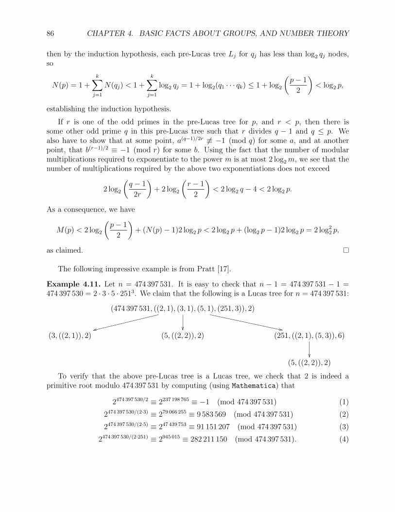
86 CHAPTER 4. BASIC FACTS ABOUT GROUPS, AND NUMBER THEORY
then by the induction hypothesis, each pre-Lucas tree Lj for qj has less than log2 qj nodes,so
N(p) = 1 +k∑j=1
N(qj) < 1 +k∑j=1
log2 qj = 1 + log2(q1 · · · qk) ≤ 1 + log2
(p− 1
2
)< log2 p,
establishing the induction hypothesis.
If r is one of the odd primes in the pre-Lucas tree for p, and r < p, then there issome other odd prime q in this pre-Lucas tree such that r divides q − 1 and q ≤ p. Wealso have to show that at some point, a(q−1)/2r 6≡ −1 (mod q) for some a, and at anotherpoint, that b(r−1)/2 ≡ −1 (mod r) for some b. Using the fact that the number of modularmultiplications required to exponentiate to the power m is at most 2 log2m, we see that thenumber of multiplications required by the above two exponentiations does not exceed
2 log2
(q − 1
2r
)+ 2 log2
(r − 1
2
)< 2 log2 q − 4 < 2 log2 p.
As a consequence, we have
M(p) < 2 log2
(p− 1
2
)+ (N(p)− 1)2 log2 p < 2 log2 p+ (log2 p− 1)2 log2 p = 2 log2
2 p,
as claimed.
The following impressive example is from Pratt [17].
Example 4.11. Let n = 474 397 531. It is easy to check that n − 1 = 474 397 531 − 1 =474 397 530 = 2 · 3 · 5 · 2513. We claim that the following is a Lucas tree for n = 474 397 531:
(474 397 531, ((2, 1), (3, 1), (5, 1), (251, 3)), 2)
ssgggggggggg
gggggggggg
g
,,XXXXXXXXXXX
XXXXXXXXXXXX
X
(3, ((2, 1)), 2) (5, ((2, 2)), 2) (251, ((2, 1), (5, 3)), 6)
(5, ((2, 2)), 2)
To verify that the above pre-Lucas tree is a Lucas tree, we check that 2 is indeed aprimitive root modulo 474 397 531 by computing (using Mathematica) that
2474 397 530/2 ≡ 2237 198 765 ≡ −1 (mod 474 397 531) (1)
2474 397 530/(2·3) ≡ 279 066 255 ≡ 9 583 569 (mod 474 397 531) (2)
2474 397 530/(2·5) ≡ 247 439 753 ≡ 91 151 207 (mod 474 397 531) (3)
2474 397 530/(2·251) ≡ 2945 015 ≡ 282 211 150 (mod 474 397 531). (4)

4.6. THE LUCAS THEOREM, PRIMES IS IN NP 87
The number of modular multiplications is: 27 in (1), 26 in (2), 25 in (3) and 19 in (4).
We have 251− 1 = 250 = 2 · 53, and we verify that 6 is a primitive root modulo 251 bycomputing:
6250/2 ≡ 6125 ≡ −1 (mod 251) (5)
6250/(2·5) ≡ 610 ≡ 175 (mod 251). (6)
The number of modular multiplications is: 6 in (5), and 3 in (6).
We have 5− 1 = 4 = 22, and 2 is a primitive root modulo 5, since
24/2 ≡ 22 ≡ −1 (mod 5). (7)
This takes one multiplication.
We have 3− 1 = 2 = 21, and 2 is a primitive root modulo 3, since
22/2 ≡ 21 ≡ −1 (mod 3). (8)
This takes 0 multiplications.
Therefore, 474 397 531 is prime.
As nice as it is, Proposition 4.48 is deceiving, because finding a Lucas tree is hard.
Remark: Pratt [17] presents his method for finding a certificate of primality in terms ofa proof system. Although quite elegant, we feel that this method is not as transparent asthe method using Lucas trees, which we adapted from Crandall and Pomerance [3]. Pratt’sproofs can be represented as trees, as Pratt sketches in Section 3 of his paper. However,Pratt uses the basic version of Lucas’ theorem, Theorem 4.45, instead of the improvedversion, Theorem 4.46, so his proof trees have at least twice as many nodes as ours.
The following nice result was first shown by V. Pratt [17] in 1975.
Theorem 4.49. The problem PRIMES (testing whether an integer is prime) is in NP.
Proof. Since all even integers besides 2 are composite, we can restrict out attention to oddintegers n ≥ 3. By Theorem 4.47, an odd integer n ≥ 3 is prime iff it has a Lucas tree.Given any odd integer n ≥ 3, since all the numbers involved in the definition of a pre-Lucastree are less than n, there is a finite (very large) number of pre-Lucas trees for n. Given aguess of a Lucas tree for n, checking that this tree is a pre-Lucas tree can be performed inO(log2 n), and by Proposition 4.48, checking that it is a Lucas tree can be done in O(log2
2 n).Therefore PRIMES is in NP.
88 CHAPTER 4. BASIC FACTS ABOUT GROUPS, AND NUMBER THEORY
Of course, checking whether a number n is composite is in NP, since it suffices to guessto factors n1, n2 and to check that n = n1n2, which can be done in polynomial time in log2 n.Therefore, PRIMES ∈ NP ∩ coNP. As we said earlier, this was the situation until thediscovery of the AKS algorithm, which places PRIMES in P.
Remark: Altough finding a primitive root modulo p is hard, we know that the number ofprimitive roots modulo p is ϕ(ϕ(p)). If p is large enough, this number is actually quite large.According to Crandal and Pomerance [3] (Chapter 4, Section 4.1.1), if p is a prime and ifp > 200560490131, then p has more than p/(2 ln ln p) primitive roots.
The Lucas test yields a method to check whether certain numbers known as Fermatnumbers are prime. These are numbers for which the prime factorization of n− 1 is a powerof 2.
Example 4.12. First, let us find a tree for n = 17. Since 17 − 1 = 16 = 24, we get theone-node tree (17, ((2, 4)), 3), where 3 is a guess for a primitive root of 17. Since
316/2 ≡ 38 ≡ −1 (mod 17),
we have a proof that 17 = 24 + 1 = 222 + 1 is prime.
Let us now find a tree for n = 257. Since 257− 1 = 256 = 28, we have the one-node tree(257, ((2, 8)), 3). We can check that
3256/2 = 3128 ≡ −1 (mod 257),
which proves that 257 = 28 + 1 = 223 + 1 is prime.
Finally, let us now find a tree for n = 65537. Since 65537 − 1 = 65536 = 216, we havethe one-node tree (65537, ((2, 16)), 3). We can check that
365536/2 = 332768 ≡ −1 (mod 65537),
which proves that 65537 = 216 + 1 = 224 + 1 is prime.
The numbers Fk = 22k + 1 are known as Fermat numbers . We just verified that F0 = 3,F1 = 5, F2 = 17, F3 = 257, and F4 = 65537, are prime.
Is Fk prime for any k ≥ 5? Since 22k grows very fast with k, this is a very hard problem.
Euler found that F5 = 232 + 1 = 4294967297 = 641 · 6700417, so F5 is not prime. Wedetermined that F2, F3, F4 are prime by applying Theorem 4.46 with a = 3. Actually, it canbe shown that the converse is true, and there is a criterion due to Pepin (1877) to determinewhether Fk is prime.
Theorem 4.50. (Pepin test) For all k ≥ 1, the Fermat number Fk = 22k + 1 is prime iff3(Fk−1)/2 ≡ −1 (mod Fk).
4.6. THE LUCAS THEOREM, PRIMES IS IN NP 89
Proof. One direction of the Pepin test follows from Theorem 4.46 with a = 3. The converse isshown using the Legendre symbol and the law of quadratic reciprocity discussed in Chapter6. The reader can skip this proof until she/he has read Chapter 6, or at least Sections 6.2and 6.5.
Assume that Fk is prime, the goal is to prove that(3
Fk
)= −1,
where(
3Fk
)is the Legendre symbol. First, observe that if k ≥ 1, we have
22k ≡ 222k−1 ≡ 42k−1 ≡ 1 (mod 3).
Consequently Fk = 22k + 1 ≡ 2 (mod 3). Since k ≥ 1, we also have Fk ≡ 1 (mod 4). Itfollows that
3− 1
2
Fk − 1
2≡ 0 (mod 2),
so by quadratic reciprocity (Theorem 6.13) and since Fk ≡ 2 (mod 3), by Proposition 6.6,since 3 ≡ 3 (mod 8), we have (
3
Fk
)=
(Fk3
)=
(2
3
)= −1.
By Euler’s criterion (Theorem 6.3), we have
3Fk−1
2 ≡(
3
Fk
)≡ −1 (mod Fk),
as claimed.
There is also a nice result restricting the kinds of prime factors that a Fermat numbermay have.
Theorem 4.51. (Euler, Lucas) For any integer n ≥ 2, every prime factor p of Fn = 22n + 1must satisfy p ≡ 1 (mod 2n+2).
Proof. Let p be a prime factor of Fn, and let h be the least positive integer such that2h ≡ 1 (mod p). Since p divides 22n + 1, we have 22n ≡ −1 (mod p), which implies thath = (2n)2 = 2n+1. By Fermat’s little theorem, 2p−1 ≡ 1 (mod p), so h being the leastpositive integer such that 2h ≡ 1 (mod p), we deduce that 2n+1 divides p− 1. Since n ≥ 2,this implies that p ≡ 1 (mod 8). By Proposition 6.6, we have(
2
p
)= 1,

90 CHAPTER 4. BASIC FACTS ABOUT GROUPS, AND NUMBER THEORY
so 2 is a quadratic residue modulo p, and by Euler’s criterion (Theorem 6.3), we have
2(p−1)/2 ≡(
2
p
)≡ 1 (mod p),
so h = 2n+1 divides (p− 1)/2, which means that p ≡ 1 (mod 2n+2).
For n = 5, it happens that the prime p = 641 = 1 + 128 · 5 = 1 + 27 · 5, so by Theorem4.51, the prime 641 is a factor of the Fermat number F5 = 225 + 1 = 232 + 1. This is howEuler found that F5 was composite.
The Pepin test and Theorem 4.51 have been used to show that F5, . . . , F24 are composite.It has also been established by other methods that F25, . . . , F32 are composite, but whetherany number Fk is prime for k ≥ 33 is a famous open problem.
It is interesting to observe that any prime factor of Fn is not a prime factor of any of itspredecessors F0, . . . , Fn−1. This is because for n ≥ 1, we have
F0F1 · · ·Fn−1 = Fn − 2,
which is easily shown by induction using the fact that
(Fn − 2)Fn = F 2n − 2Fn
= (22n + 1)2 − 2(22n + 1)
= 22n+1
+ 222n + 1− 222n − 2
= 22n+1 − 1 = Fn+1 − 2.
Any prime factor of Fn and Fj for j < n would divide 2, but the Fk are odd, so this isimpossible. As a corollary we obtain an amusing proof of the fact that there are infinitelymany primes.
For more on Fermat numbers, see Crandal and Pomerance [3] (Chapter 1, Section 1.3.2).
4.7 The Structure of Finite Fields
Suppose K is a field of characteristic p. For every i, with 0 ≤ i ≤ p, the binomial coefficient(pi
)is given by (
p
i
)=
p!
i!(p− i)!,
so if 1 ≤ i ≤ p− 1, we have
i
(p
i
)= p
(p− 1
i− 1
).
Since 1 ≤ i ≤ p− 1 and p is prime, we have gcd(p, i) = 1, and so p divides(pi
).
4.7. THE STRUCTURE OF FINITE FIELDS 91
Proposition 4.52. If K is a field of characteristic p, the map (Frobenius map) σ : K → Kgiven by
σ(a) = ap
is an isomorphism of K onto a subfield of K denoted Kp.
Proof. Since K is commutative, it is clear that σ(ab) = σ(a)σ(b). Obviously σ(0) = 0 andσ(1) = 1. By the binomial formula and using the fact that p divides
(pi
)for i = 1, . . . , p− 1,
since K has characteristic p, we have(pi
)= 0 for i = 1, . . . , p− 1, so we have
σ(a+ b) = (a+ b)p
= ap +
p−1∑i=1
(p
i
)ap−ibi + bp
= ap + bp = σ(a) + σ(b).
Therefore, σ is a homomorphism, and as we remarked earlier, it is injective.
The field Z/pZ with p prime is also denoted by Fp. Here is the structure theorem forfinite fields (after J.P. Serre; see Serre [20]).
Theorem 4.53. Let K be a finite field.
(i) The field K is of characteristic p ≥ 2 (p prime). If K is of degree m over Fp, then Khas q = pm elements.
(ii) Let p be any prime, let m be any natural number m ≥ 1, and write q = pm. For anyalgebraicaly closed field Ω of characteristic p, there exists a unique subfield Fq of Ω withq elements. The map σq : Ω → Ω given by σq(x) = xq is an automorphism of Ω, andthe field Fq is the set of roots of the polynomial Xq −X; that is, Fq = Fix(σq).
(iii) Every finite field with q = pm elements is isomorphic to Fq.
Proof. (i) Since K is finite, the map Z −→ K given by n 7→ n · 1 cannot be injective, so Kmust have characteristic p ≥ 2, and it contains Fp as a subfield. If K has dimension m as avector space over Fp, then it is obvious that K has pm elements.
(ii) We know from Proposition 4.52 that the map σ : Ω → Ω given by σ(x) = xp is aninjective homomorphism. Since σq = σm, the map σq is also an injective homomorphism.Since Ω is algebraically closed, for any a ∈ K, the polynomial Xq − a has a root in Ω, whichshows that σq is also surjective, thus an automorphism of Ω. Then, the field Fq fixed by σqis a subfield of Ω. Since Fq is also the set of roots of the polynomial Xq −X, it has at mostq roots. We claim that F (X) = Xq −X has simple roots. From a result of algebra, this isthe case if the derivative F ′(X) of F (X) is not the zero polynomial. But, since we are incharacteristic p and m ≥ 1, we have
F ′(X) = qXq−1 − 1 = ppm−1Xq−1 − 1 = −1
92 CHAPTER 4. BASIC FACTS ABOUT GROUPS, AND NUMBER THEORY
so F ′(X) is not zero. Therefore, F (X) has exactly q roots, and Fq has q = pm elements.
If K is any other subfield of Ω with q elements, since the multiplicative group K∗ of Kis a finite group of order q − 1, we have
xq−1 = 1, for all x ∈ K∗,
and soxq − x = 0 for all x ∈ K,
which shows that K is fixed by σq, and so K ⊆ Fq. Since |K| = |Fq| = q, we must haveK = Fq.
(iii) If K is a finite field with q = pm elements, then the reasoning in (ii) shows that Kis the set of roots of the polynomial F (X) = Xq − X. This means that K is the splittingfield of Fp (the smallest field extension of Fp in which F (X) has all its roots). But, as Ω isalgebraically closed and contains a copy of Fp, it contains a splitting field K ′ of Fp. Since anytwo splitting fields are isomorphic (see Lang [11], Chapter 5), the field K can be embeddedin Ω (as K ′), so by (ii) K is isomorphic to Fq.
Using Theorem 4.22, we obtain the following important result.
Theorem 4.54. For every prime p and every integer m ≥ 1, the multiplicative group F∗pmof the finite field Fpm is a cyclic group with pm − 1 elements.
Proof. For any divisor d of pm − 1, the polynomial Xd − 1 has at most d roots in F∗pm ,therefore by Theorem 4.22, the group F∗pm is cyclic.
Any generator of F∗pm is called a primitive root of unity (to be more precise, a primitive(pm− 1)th root of unity). Observe that the proof of Theorem 4.54 actually shows that everyfinite subgroup of the multiplicative subgroup K∗ of any field K is cyclic.

Chapter 5
The Miller–Rabin Test
This chapter is heavily inspired by Dietzfelbinger [4] and Crandall and Pomerance [3]. TheMiller–Rabin test makes use of two basic properties of the prime numbers:
(1) Fermat’s little theorem, which says that if p is a prime and if a is any integer which isnot a multiple of p, then
ap−1 ≡ 1 (mod p).
Usually, we assume that 1 ≤ a ≤ p− 1.
(2) If p is a prime, then 1 has only trivial square roots, which means that the only solutionsa with 1 ≤ a ≤ p− 1 of the congruence
a2 ≡ 1 (mod p)
are a = 1 and a = p− 1 ≡ −1 (mod p).
Property (2) is proved as follows.
Proof. Observe that if a2 ≡ 1 (mod p), then a2 − 1 = (a + 1)(a − 1) is divisible by p, andsince p is prime, either p divides a − 1 or p divides a + 1. Because 1 ≤ a ≤ p − 1, weconclude that a = 1 or a = p − 1. On the other hand, 1 and p − 1 are always square rootsof unity modulo p (even if p is not prime), since 12 ≡ 1 (mod p) and (p − 1)2 ≡ (−1)2 ≡ 1(mod p).
Since computing a mod n is cheap, a first approach to test whether a number n is primeis to see if (2) fails. To understand how practical this method is, we need to know how manysquare roots modulo n the equation x2 ≡ 1 (mod n) has. This is the purpose of the nextsection.
Recall that if n ≥ 2, the group (Z/nZ)∗ is the multiplicative group of units of the ringZ/nZ; that is,
(Z/nZ)∗ = a ∈ N | 1 ≤ a ≤ n− 1, gcd(a, n) = 1.
93

94 CHAPTER 5. THE MILLER–RABIN TEST
Here and in several places later, with a slight abuse of notation, we are identifying theequivalence class a of a with its representative a mod n. The order (number of elements)of (Z/nZ)∗ is ϕ(n), where ϕ(n) is the number of integers a, with 1 ≤ a ≤ n, which arerelatively prime to n (gcd(a, n) = 1).
5.1 Square Roots of Unity
It turns out that 1 and −1 are the only square roots of unity modulo n iff n is of the form 4,pm, or 2pm, where p is an odd prime.1 To prove this fact, we use the following proposition.
Proposition 5.1. If p is an odd prime, then there are exactly two square roots of unitymodulo pm and 2pm (m ≥ 1), namely 1 and −1. There is a unique square root of unitymodulo 2 (i.e. 1), two square roots of unity modulo 4 (i.e. ±1), and four square root of unitymodulo 2m if m ≥ 3, namely ±1 and 2m−1 ± 1.
Proof. If x2 ≡ 1 (mod n), then x is its own invere modulo n, so x mod n ∈ (Z/nZ)∗, andwe may assume that x ∈ (Z/nZ)∗. First, assume that n = pm with p an odd prime. Inthis case, we know that primitive roots modulo pm exist, so pick one, say g. Then, everyx ∈ (Z/pmZ)∗ can be written as x = gi, with 1 ≤ i ≤ ϕ(pm) = pm−1(p − 1), and x2 ≡ 1(mod pm) is equivalent to g2i ≡ 1 (mod pm). Since g has order ϕ(pm), the congruence g2i ≡ 1(mod pm) holds iff ϕ(pm) = pm−1(p− 1) divides 2i, that is, iff pm−1(p− 1)/2 divides i (sincep is odd). Since 1 ≤ i ≤ pm−1(p− 1), there are only two possibilities: i = pm−1(p− 1)/2 andi = pm−1(p− 1), which correspond to x = −1 and x = 1.
The case n = 2pm is analogous, since primitive roots also exist and since ϕ(2pm) = ϕ(pm).
The cases n = 2 and n = 4 are clear.
Assume that n = 2m with m ≥ 3. We are seeking solutions of the congruence x2 ≡ 1(mod 2m), with 1 ≤ x ≤ 2m − 1. Note that
(2m−1 + x)2 ≡ 22m−2 + 2mx+ x2 ≡ x2 (mod 2m)
since m ≥ 3. Therefore, it is sufficient to find solutions x such that 1 ≤ x ≤ 2m−1 − 1. Wehave x2 ≡ 1 (mod 2m) iff (x− 1)(x+ 1) ≡ 0 (mod 2m), so there are three mutally exclusivepossibilities:
1. x ≡ 1 (mod 2m). Since 1 ≤ x ≤ 2m − 1, we must have x = 1.
2. x ≡ −1 ≡ 2m − 1 (mod 2m). Since 1 ≤ x ≤ 2m−1 − 1, this case is impossible.
3. x− 1 = h2i and x+ 1 = k2m−i, with 1 ≤ i ≤ m− 2 and h, k > 0.
1I thank Peter Freyd for communicating this result to me.

5.1. SQUARE ROOTS OF UNITY 95
In the third case, we deduce that
x = h2i−1 + k2m−i−1
1 = k2m−i−1 − h2i−1.
If 2 ≤ i ≤ m− 2, then 1 is divisible by 2, which is absurd. Therefore i = 1.
If i = 1, since x+1 = k2m−i, we have x = k2m−1−1, and since k > 0 and 1 ≤ x ≤ 2m−1−1,we must have k = 1, so
x = 2m−1 − 1.
Since m ≥ 3, we have 2m−1−1 6≡ 1 (mod 2m), and 2m−1−1 is a square root of unity distinctfrom 1.
In summary, we proved that there are exactly two square roots of unity x = 1 andx = 2m−1 − 1 such that 1 ≤ x ≤ 2m−1 − 1. Since x + 2m−1 is also a square root of unity,2m−1 + 1 and 2m−1 + 2m−1 − 1 = 2m − 1 ≡ −1 (mod m), are also squares roots of unity, sothere are exactly four square roots of unity modulo 2m; namely ±1 and 2m−1 ± 1.
Remark: The fact that there are precisely four square roots of unity modulo 2m when m ≥ 3follows immediately from the fact that (Z/2mZ)∗ is isomorphic to the direct product of thetwo cyclic subgroups −1, 1 and 〈5〉, both of even order (see Theorem 4.44).
Now, we can determine the exact number of square roots of unity modulo n.
Theorem 5.2. For any natural number n > 1, if the prime factorization of n is
n = 2mpj11 · · · pjkk ,
where p1, . . . , pk are distinct odd primes and m+ k ≥ 1, then the number s of disinct squareroots of unity modulo n is given by
s =
2k if m = 0 and k ≥ 1 or m = 1 and k ≥ 0
2k+1 if m = 2 and k ≥ 0
2k+2 if m ≥ 3 and k ≥ 0.
Proof. First, consider the case where m = 0. Since p1, . . . , pk are pairwise relatively prime,the congruence x2 ≡ 1 (mod n) is equivalent to the k congruences
x2 ≡ 1 (mod pj11 )
...
x2 ≡ 1 (mod pjk1 ).
From Proposition 5.1, each congruence x2 ≡ 1 (mod pji1 ) has the two solutions x = 1 andx = −1 modulo pj
ji . By the Chinese remainder theorem, there is a bijection between the
96 CHAPTER 5. THE MILLER–RABIN TEST
set of solutions x modulo n and the set of k tuples of solutions (x1, . . . , xk) where xi is asolution modulo pj
ji , and since there are 2k solutions (x1, . . . , xk) with xi = ±1, there are 2s
square roots modulo n.
If k = 0, then Proposition 5.1 says that the congruence x2 ≡ 1 (mod 2m) has one solutionif m = 1, two solutions if m = 2, and 4 solutions if m ≥ 3.
If m ≥ 1 and k ≥ 1, since 2, p1, . . . , pk are pairwise relatively prime, the congruencex2 ≡ 1 (mod n) is equivalent to the k + 1 congruences
x2 ≡ 1 (mod 2m)
x2 ≡ 1 (mod pj11 )
...
x2 ≡ 1 (mod pjk1 ).
Again, we use the Chinese remainder theorem. Each congruence x2 ≡ 1 (mod pji1 ) has thetwo solutions 1 and −1, and the congruence x2 ≡ 1 (mod 2m) has one solution if m = 1, twosolutions if m = 2, and 4 solutions if m ≥ 3. Therefore, there are 2k square roots if m = 1,2× 2k = 2k+1 square roots if m = 2, and 4× 2k = 2k+2 square roots if m = 3.
For example, if n = 91 = 7× 13, then 272 = 729 = 8× 91 + 1, so 27 is a square root of 1(mod 91). The other nontrivial square root of 1 (mod 91) is 64.
If we find some nontrivial square root of unity a modulo n, then we know that n is com-posite (and a is a witness to the fact that n is composite). Unfortunately, if n is composite,unless the number k of distinct primes dividing n is large, the number of nontrivial squareroots of unity modulo n (at most 2k+2 − 2) is a lot smaller than n, so it is not practical totest a randomly chosen a ∈ 2, . . . , n − 2. Therefore we consider making use of (1) for amore practical test.
5.2 The Fermat Test; F -Witnesses and F -Liars
Going back to (1), observe that if n ≥ 2, then by the binomial formula, we have
(n− 1)n−1 ≡ (−1)n−1 (mod n).
Consequently, if n ≥ 3 is odd, then
(n− 1)n−1 ≡ 1 (mod n),
and if n ≥ 4 is even, then
(n− 1)n−1 ≡ −1 (mod n).

5.2. THE FERMAT TEST; F -WITNESSES AND F -LIARS 97
(In the special case where n = 2, we have 1 ≡ −1 (mod 2).) Now, for any natural numbern ≥ 4, if 2 ≤ a ≤ n− 2 and if
an−1 6≡ 1 (mod n),
then n is not prime, since Fermat’s little theorem does not hold. Since all primes except 2are odd integers, we only need to test odd integers for compositeness and this suggests thefollowing test:
Fermat test: For any odd integer n ≥ 5, pick randomly some a ∈ 2, . . . , n− 2.If an−1 6≡ 1 (mod n), then return “n is composite,” else return “n is a probable prime.”
Of course, we compute exponentiation modulo n using fast algorithms based on repeatedsquaring.
Definition 5.1. Let n ∈ N be any integer such that n ≥ 3.
(1) An integer a such that 2 ≤ a ≤ n−1 is called a Fermat witness , for short an F -witnessfor n, if an−1 6≡ 1 (mod n).
(2) If n is an odd composite, then an integer a with 1 ≤ a ≤ n − 1 is a Fermat liar , forshort an F -liar for n, if an−1 ≡ 1 (mod n). The set of F -liars for n is denoted by LFn .
Every even number n ≥ 4 has n− 1 has an F -witness. This is a bit of an overkill, sinceevery positive even number, except 2, is a composite. The number 1 is a trivial F -liar, andby a previous observation, when n is an odd composite, n− 1 is always an F -liar.
Definition 5.2. A composite number n ≥ 4 such a ≥ 2 is an F -liar for n is called a Fermatpseudoprime base a (for short, a pseudoprime base a).
It can be checked that 2 is an F -witness for all integers n ≥ 3 up to n = 340. However,for n = 341 = 11× 31, we get
2340 ≡ 1 (mod 341),
so 2 is an F -liar for 341, and 341 is a pseudoprime base 2. If we try a = 3, we find that
3340 ≡ 56 (mod 341),
so 3 is an F -witness for 341, and 341 is not a pseudoprime base 3. On the other hand, it iseasy to check that 91 = 7× 13 is not a pseudoprime base 2 because 290 ≡ 64 (mod 91), butit is a pseudoprime base 3 because 390 ≡ 1 (mod 91).
The above considerations suggest the following question: if n ≥ 3 is a (odd) composite,does it necessarily have some F -witness? The answer is yes, but this is not of practical use.
Proposition 5.3. For any integer n ≥ 2, the following properties hold:
(a) For any integer a such that 1 ≤ a ≤ n − 1, if ar ≡ 1 (mod n) for some r ≥ 1, thena ∈ (Z/nZ)∗.
98 CHAPTER 5. THE MILLER–RABIN TEST
(b) If an−1 ≡ 1 (mod n) for all a with 1 ≤ a ≤ n− 1, then n is prime.
Proof. (a) if r = 1, then we must have a = 1, and if r ≥ 2, then ar−1a ≡ 1 (mod n) showsthat a is a unit, so in both cases a ∈ (Z/nZ)∗.
(b) If an−1 ≡ 1 (mod n) for all a with 1 ≤ a ≤ n − 1, then by (a), we have (Z/nZ)∗ =1, . . . , n− 1, so gcd(a, n) = 1 for all a = 2, . . . , n− 1, which implies that n is prime.
By Proposition 5.3 (b), if n ≥ 4 is a composite, then it must have some F -witness.Furthermore, by (a), the n− 1− ϕ(n) elements of the set
1, . . . , n− 1 − (Z/nZ)∗ = a ∈ N | 2 ≤ a ≤ n− 2 | gcd(a, n) > 1
must be all F -witnesses (an−1 6≡ 1 (mod n)).
Unfortunately, this set is very slim for many composite numbers. For example, if n = pqis the product of two distinct primes p and q, then this sets contains pq−1− (p−1)(q−1) =p+ q − 2 elements. If p and q are roughly equal, then p+ q − 2 is very small in comparisonto n = pq.
The case n = 91 = 7 × 13 gives us a concrete idea of what is going on. There are 18F -witnesses not in (Z/91Z)∗ (multiples of 7 and 13):
7, 14, 21, 28, 35, 42, 49, 56, 63, 70, 77, 84
13, 26, 39, 52, 65, 78.
There are 36 F -witnesses in (Z/91Z)∗:
2, 5, 6, 8, 11, 15, 18, 19, 20, 24, 31, 32,
33, 34, 37, 41, 44, 45, 46, 47, 50, 54, 57, 58,
59, 60, 67, 71, 72, 73, 76, 80, 83, 85, 86, 89.
Finally, there and 36 F -liars (necessarily in (Z/91Z)∗);
1, 3, 4, 9, 10, 12, 16, 17, 22, 23, 25, 27,
29, 30, 36, 38, 40, 43, 48, 51, 53, 55, 61, 62,
64, 66, 68, 69, 74, 75, 79, 81, 82, 87, 88, 90.
The Fermat test gives the wrong answer if the random choice for a hits one the 34 F -liarsother and 1 and 90, which has probabilty 34/88 = 17/44. Observe that 17/34 < 1/2. Thisis a general fact, provided that the odd composite n has some F -witness in (Z/nZ)∗. Thisfollows from the interesting fact that the set LFn of F -liars is a subgroup of (Z/nZ)∗.
Proposition 5.4. For any integer n ≥ 2, the set LFn of F -liars is a subgroup of (Z/nZ)∗.Furthermore, if n is an odd composite and if n possesses at least some F -witness in (Z/nZ)∗,then the probability that the Fermat test gives the wrong answer, more precisely the probabilitythat any a ∈ 2, . . . , n− 2 is an F -liar for n, is at most 1/2.

5.3. CARMICHAEL NUMBERS 99
Proof. Since 1 ≡ 1 (mod n), we have 1 ∈ LFn . Since (Z/nZ)∗ is a finite group, to show thatLFn is a subgroup, it suffices to show closure under multiplication. If an−1 ≡ 1 (mod n) andbn−1 ≡ 1 (mod n), then (ab)n−1 ≡ an−1bn−1 ≡ 1 (mod n), as desired.
By Lagrange’s theorem, the order |LFn | of LFn divides the order ϕ(n) of (Z/nZ)∗. Ifthere is some F -witness in (Z/nZ)∗, then LFn is a proper subgroup of (Z/nZ)∗. Since n is acomposite and since LFn is a proper subgroup, we deduce that ϕ(n) < n− 1 and that |LFn | isa proper divisor of ϕ(n), which implies that
|LFn | ≤ (n− 2)/2.
Thus, the probability that some a chosen in 2, . . . , n − 2 belongs to LFn − 1, n − 1 isbounded by
(n− 2)/2− 2
n− 3=
n− 6
2(n− 3)<
1
2,
since 2n− 12 < 2n− 6.
The good news about Proposition 5.4 is that if n is an odd composite and if n has someF -witness in (Z/nZ)∗, then the probability that the Fermat test gives the wrong answer isless than 1/2. By repeating the test ` times, each time choosing randomly and independentlysome a in 2, . . . , n− 2, we can make the probability of failure less than (1/2)`.2
5.3 Carmichael Numbers
The bad news is that there exist odd composites n such that LFn = (Z/nZ)∗; that is, n hasno F -witness in (Z/nZ)∗. The smallest such number is 561 = 3× 11× 17. This number is apseudoprime in any base relatively prime to 561. Such “nasty” numbers were first discoveredby R. Carmichael in 1910, and motivates the following definition.
Definition 5.3. An integer n ≥ 3 for which an−1 ≡ 1 (mod n) for all a ∈ 2, . . . , n − 1,with gcd(a, n) = 1, is called a probable prime. A composite integer n ≥ 3 which is a probableprime is called a Carmichael number .
If n ≥ 4 is even, we observed that n− 1 is an F -witness for n, so a Carmichael numbermust be odd.
2We have to be careful about which probability we are talking about. In this case, we are considering theconditional probability that the algorithm lies ` times (fails to report that n is composite), given that n iscomposite. However, as a user of the algorithm, it is more useful to know the conditional probability that nis composite, given that the algorithm runs ` times and each time fails to report that n is composite. Thetwo conditional probabilities are related by Bayes’s formula. The second conditional probability involves thedensity of primes. A computation shows that the probability (1/2)` must be (approximately) multiplied bylnn. We will come back to this point later on.

100 CHAPTER 5. THE MILLER–RABIN TEST
Unfortunately for primality testing, there are infinitely many Carmichael numbers. Thisfact was proved in 1994 by Alford, Granville and Pomerance. They also proved that there issome integer x0 > 0, such that for all x ≥ x0, the number C(x) of Carmichael numbers notexceeding x satisfies C(x) > x2/7.
Remark: The sufficiently large x0 is not known explicitly, but it is conjectured that it isthe 96th Carmichael number: 8719309.
Other authors define a Carmichael number as a composite integer n ≥ 3 for which
an ≡ a (mod n) for all a ∈ N.
This second definition implies the first (Definition 5.3), because if an ≡ a (mod n) and ifgcd(a, n) = 1, then we can divide by a and we obtain an−1 ≡ 1 (mod n). Definition 5.3implies the second definition, but this requires a little work. We can use of a criterion dueto A. Korselt. This criterion was found in 1899, eleven years before Carmichael actuallyproduced the first example. Presumably Korselt believed that such numbers did not exist,and he developed a criterion as a first step in proving this.
Theorem 5.5. (Korselt criterion) An integer n ≥ 2 is a Carmichael number iff the followingtwo conditions hold.
(1) The number n is composite and not divisible by the square of any prime (it is square-free).
(2) For every prime p, if p divides n then p− 1 divides n− 1.
Proof. First, let n be a Carmichael number.
(1) Assume that n is divisible by the square of some prime p. Since n must be odd, wecan write n = pkm, where p ≥ 3 is a prime, k ≥ 2, and p does not divide m. We produce anF -witness in (Z/nZ)∗ for n as follows:
Case 1. If m = 1, let a = p + 1. Clearly, gcd(p + 1, pk) = 1. We claim that an−1 6≡ 1(mod n). We proceed by contradiction. If an−1 ≡ 1 (mod n), then since p2 divides n, wehave an−1 ≡ 1 (mod p2). However, by the binomial formula, we have
an−1 ≡ (1 + p)n−1 ≡ 1 + (n− 1)p+n−1∑i=2
(n− 1
i
)pi ≡ 1 + (n− 1)p (mod p2).
Since an−1 ≡ 1 (mod p2), we deduce that (n − 1)p ≡ 0 (mod p2), which means that p2
divides (n− 1)p, and since p is prime, p divides n− 1. However, n− 1 = pk − 1 with k ≥ 2,so p does not divide n− 1, a contradiction.
Case 2. If m ≥ 3, then we use the Chinese remainder theorem to find some a with1 ≤ a < p2m ≤ n so that
a ≡ p+ 1 (mod p2)
a ≡ 1 (mod m).

5.3. CARMICHAEL NUMBERS 101
Since p2 divides a − (p + 1), the prime p does not divide a, so gcd(a, pk) = 1. Sincea ≡ 1 (mod m), we also have gcd(a,m) = 1. Because gcd(pk,m) = 1 and n = pkm, weconclude that gcd(a, n) = 1. We claim that an−1 6≡ 1 (mod n). As in Case 1, we proceedby contradiction. Then, by the same reasoning, we deduce that p divides n− 1. This time,n− 1 = pkm− 1, and again p does not divide n− 1, a contradiction.
(2) By (1), n is a product of distinct primes. Assume that the prime p divides n. Sincep is prime, the group (Z/pZ)∗ is cyclic (see Theorem 4.34) so pick a generator g (a primitiveroot modulo p). By the Chinese remainder theorem, we can find some b such that
b ≡ g (mod p)
b ≡ 1 (mod n/p).
Since n is a product of distinct primes, the numbers p and n/p have no common factor, sogcd(b, n) = 1. Since n is a Carmichael number, we have
bn−1 ≡ 1 (mod n),
and since p divides n, we get
gn−1 ≡ bn−1 ≡ 1 (mod p).
Since g has order p− 1, the number p− 1 divides n− 1.
Conversely, assume that (1) and (2) hold. Let a ∈ 1, . . . , n − 1 be any integer suchthat gcd(a, n) = 1. For any prime p dividing n, we also have gcd(a, p) = 1, so by Fermat’slittle theorem,
ap−1 ≡ 1 (mod p).
Since p− 1 divides n− 1, we also have
an−1 ≡ 1 (mod p).
Since the prime factors of n are all distinct, we deduce that
an−1 ≡ 1 (mod n),
which shows that n is a Carmichael number.
Suppose n is a Carmichael number. Then by Korselt’s criterion (Proposition 5.5) Condi-tions (1) and (2) hold. If gcd(a, p) = 1, then the proof of (2) shows that an−1 ≡ 1 (mod p),thus an ≡ a (mod p). If p divides a then an ≡ a (mod p) holds trivially (since p dividesn). Therefore an ≡ a (mod p) for all a, and since the prime factors of n are all distinct, weconclude that
an ≡ a (mod n) for all n ∈ N.
We saw in Theorem 5.5 that every Carmichael numbers contains distinct prime factors.The number of distinct prime factors must be at least three.

102 CHAPTER 5. THE MILLER–RABIN TEST
Proposition 5.6. Every Carmichael number contains at least three distinct prime factors.
Proof. We make use of Theorem 5.5. Assume that some Carmichael number n is the productof two distinct primes p and q. We may suppose that 3 ≤ p < q. By Theorem 5.5, Property(2) says that p− 1 and q − 1 both divide n− 1. But, n− 1 = pq − 1 = p(q − 1) + p− 1, son−1 ≡ p−1 (mod (q−1)), and p−1 6≡ 0 (mod (q−1)) since q > p ≥ 3, a contradiction.
Here is a list of the first ten smallest Carmichael numbers; see Ribenboim [18] (Chapter2, Section IX):
651 = 3 · 11 · 17
1105 = 5 · 13 · 17
1729 = 7 · 13 · 19
2465 = 5 · 17 · 29
2821 = 7 · 13 · 31
6601 = 7 · 23 · 41
8911 = 7 · 19 · 67
10585 = 5 · 29 · 73
15841 = 7 · 31 · 73
29341 = 13 · 37 · 61.
If n is a Carmichael number, then LFn = (Z/nZ)∗, so the set 1, . . . , n− 1 − (Z/nZ)∗ ofF -witnesses is quite thin, and the probability that the Fermat test gives the wrong answer(n is prime) is
ϕ(n)− 2
n− 3>ϕ(n)
n=
∏p is prime
p|n
(1− 1
p
).
This bound is annoyingly close to 1 if n has only few large prime factors. For example, if nis the Carmichael number
n = 651693055693681 = 72931× 87517× 102103,
we find that ϕ(n)/n > 0.99996. Repeating the test does not help, because if n has only 3or 4 factors and if the smallest prime factor is p0, then it is not hard to see that we wouldhave to repeat the test a number of times proportional to p0 to make the error probabilityless than 1/2. Therefore, a new idea is necessary to break the curse of Carmichael numbers.
5.4. THE MILLER–RABIN TEST; MR-WITNESSES AND MR-LIARS 103
5.4 The Miller–Rabin Test; MR-Witnesses and MR-
Liars
The new idea is to make use of the nontrivial square root of unity test. If n ≥ 3 is an oddinteger, we can factor the largest power of 2 in n− 1; that is, we write
n− 1 = 2kt,
where t is odd. The point is that if p is prime, then for any a which is not a multiple of p,the residues of at and a2
it (with 0 ≤ i ≤ k−1) modulo p must satisfy some special condition.
Proposition 5.7. Let p be an odd prime, and write
p− 1 = 2kt, with t odd and k ≥ 1.
For any natural number a which is not a multiple of p, one of the following two conditionsmust hold:
(1) either at ≡ 1 (mod p),
(2) or a2it ≡ n− 1 (mod p), for some i with 0 ≤ i ≤ k − 1.
Proof. By Fermat’s little theorem, we have
ap−1 ≡ 1 (mod p),
that isa2
kt ≡ 1 (mod p).
This implies that if we consider the list
b0 = at, b1 = a2t, b2 = a22t, . . . , bk−1 = a2
k−1t, bk = a2kt = an−1,
the last number is congruent to 1 modulo p, and since
a2i+1t =
(a2
it)2,
we have bi+1 = b2i , for i = 0, . . . , k − 1. There are only two possibilities:
(i) We have b0 = at ≡ 1 (mod p).
(ii) There is some bi such that bi 6≡ 1 (mod p), but b2i ≡ 1 (mod p), for some i with0 ≤ i ≤ k− 1. Because n is prime, we know that b2i ≡ 1 (mod p) implies that bi ≡ ±1(mod p), and since +1 is ruled out, we must have bi ≡ −1 ≡ n− 1 (mod p).
Case (i) corresponds to Case (1) and Case (ii) corresponds to Case (2).

104 CHAPTER 5. THE MILLER–RABIN TEST
Observe that Condition (2) for i = 0 says that at ≡ n − 1 (mod n), or equivalentlyat ≡ −1 (mod n). Proposition 5.7 implies that if we can find some natural number a such
that
(a) at 6≡ ±1 (mod n), and
(b) a2it 6≡ n− 1 (mod n), for all i with 1 ≤ i ≤ k − 1,
then n must be a composite.
Indeed, if a satisfies both properties (a) and (b) above, then a is not a multiple of n, sinceotherwise we would have at ≡ 0 (mod n) and a2
it ≡ 0 (mod n) for all i with 1 ≤ i ≤ k − 1,so (a) and (b) would not hold. Then, by the contrapositive of Proposition 5.7, the numbern can’t be prime.
Clearly, a 6= 1, but a 6= n−1 as well, since (n−1)t ≡ −1, because t is odd. Furthermore,if a ∈ 2, . . . , n−2 then we may assume that gcd(a, n) = 1, since otherwise 2 ≤ gcd(a, n) ≤n− 2, and n is composite.
The above leads to to the following definition.
Definition 5.4. Let n ≥ 3 be any odd integer, and write n− 1 = 2kt, with k ≥ 1 and t odd.
(1) A number a such that 2 ≤ a ≤ n− 2 with gcd(a, n) = 1 is a Miller–Rabin witness , forshort a MR-witness for n, if the following two conditions hold:
(a) at 6≡ ±1 (mod n), and
(b) a2it 6≡ n− 1 (mod n), for all i with 1 ≤ i ≤ k − 1.
(2) If n is composite, then any integer a with 1 ≤ a ≤ n− 1 is Miller–Rabin liar , for shortan MR-liar for n, iff a is not an MR-witness for n. The set of MR-liars for n is denotedby LMR
n , and we have
LMRn = a ∈ 1, . . . , n− 1, either at ≡ 1 (mod n),
or a2it ≡ n− 1 (mod n), for some i with 0 ≤ i ≤ k − 1.
The numbers a = 1 and a = n − 1 are trivial MR-liars. Observe that every MR-liar isan F -liar: If at ≡ 1 (mod n), then
an−1 ≡(at)2k ≡ (1)2
k ≡ 1 (mod n),
and if a2it ≡ n− 1 (mod n), for some i with 0 ≤ i ≤ k − 1, then
an−1 ≡(a2
it)2k−i
≡ (−1)2k−i ≡ 1 (mod n),
since i ≤ k − 1.

5.4. THE MILLER–RABIN TEST; MR-WITNESSES AND MR-LIARS 105
Thus, LMRn ⊆ LFn , but unfortunately, LMR
n is not a group. For example, if n = 325 =52 × 13, then n− 1 = 22 × 81, and it is easy to verify that
72×81 ≡ 324 (mod 325)
322×81 ≡ 324 (mod 325)
22481 ≡ 274 (mod 325)
2242×81 ≡ 1 (mod 325)
22422×81 ≡ 1 (mod 325),
so 7 and 32 are both MR-liars, but their product 224 is a MR-witness. When n is not aCarmichael number, LMR
n is contained in LFn which is a proper subgroup of (Z/nZ)∗, so theproportion of MR-liars is less than 1/2, but when n is a Carmichael number, we need to findanother proper subgroup of (Z/nZ)∗ containing LMR
n . Fortunately, this is possible.
Definition 5.5. An odd composite number n such that a with 2 ≤ a ≤ n− 2 is an MR-liarfor n is called a strong pseudoprime base a.
Because every MR-liar is an F -liar, every strong pseudoprime base a is a pseudoprimebase a. The converse is false.
The number 91 is an example of a pseudoprime base 10 which is also a strong pseudoprimebase 10. Indeed, 90 = 2× 45, and 1045 ≡ 90 (mod 91), which shows that 10 is an MR-liar.
We saw earlier that n = 341 is a pseudoprime base 2. But 341 is not a strong pseudoprimebase 2, because 340 = 22 × 85, 285 ≡ 32 (mod 341), and 22×85 ≡ 1 (mod 341), so 2 is anMR-witness for 341. In fact, 32 is a nontrivial square root of unity modulo 341.
The Carmichael number n = 561 = 3× 11× 17 is a pseudoprime for every base relativelyprime to 561, and 560 = 24 × 35. For a = 2, we obtain
235 ≡ 263 (mod 561)
22×35 ≡ 2632 ≡ 166 (mod 561)
222×35 ≡ 1662 ≡ 67 (mod 561)
223×35 ≡ 672 ≡ 1 (mod 561)
Since 263 6≡ ±1 (mod 561), and 166, 67, 1 6≡ 560 (mod 561), the number 2 is an MR-witnessfor 561, which is not a strong pseudoprime base 2.
Here is another example from Hoffstein, Pipher and Silverman [8] (Chapter 3, Section3.4). We leave it as an exercise to check that if n = 172947529, then n− 1 = 23× 21618441,and with a = 17, we get
1721618441 ≡ 1 (mod 172947529),
so 17 is not an MR-witness for 172947529. With a = 3, we get
321618441 ≡ −1 (mod 172947529),
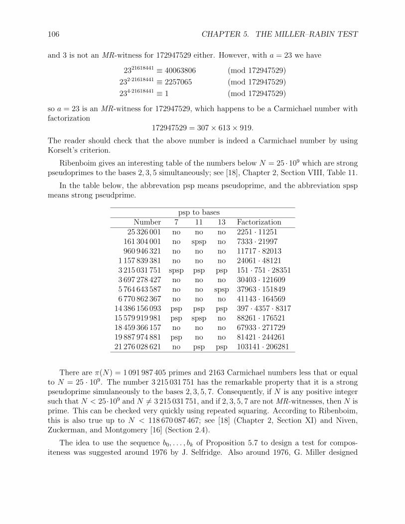
106 CHAPTER 5. THE MILLER–RABIN TEST
and 3 is not an MR-witness for 172947529 either. However, with a = 23 we have
2321618441 ≡ 40063806 (mod 172947529)
232·21618441 ≡ 2257065 (mod 172947529)
234·21618441 ≡ 1 (mod 172947529)
so a = 23 is an MR-witness for 172947529, which happens to be a Carmichael number withfactorization
172947529 = 307× 613× 919.
The reader should check that the above number is indeed a Carmichael number by usingKorselt’s criterion.
Ribenboim gives an interesting table of the numbers below N = 25 · 109 which are strongpseudoprimes to the bases 2, 3, 5 simultaneously; see [18], Chapter 2, Section VIII, Table 11.
In the table below, the abbrevation psp means pseudoprime, and the abbreviation spspmeans strong pseudprime.
psp to basesNumber 7 11 13 Factorization
25 326 001 no no no 2251 · 11251161 304 001 no spsp no 7333 · 21997960 946 321 no no no 11717 · 82013
1 157 839 381 no no no 24061 · 481213 215 031 751 spsp psp psp 151 · 751 · 283513 697 278 427 no no no 30403 · 1216095 764 643 587 no no spsp 37963 · 1518496 770 862 367 no no no 41143 · 164569
14 386 156 093 psp psp psp 397 · 4357 · 831715 579 919 981 psp spsp no 88261 · 17652118 459 366 157 no no no 67933 · 27172919 887 974 881 psp no no 81421 · 24426121 276 028 621 no psp psp 103141 · 206281
There are π(N) = 1 091 987 405 primes and 2163 Carmichael numbers less that or equalto N = 25 · 109. The number 3 215 031 751 has the remarkable property that it is a strongpseudoprime simulaneously to the bases 2, 3, 5, 7. Consequently, if N is any positive integersuch that N < 25·109 and N 6= 3 215 031 751, and if 2, 3, 5, 7 are not MR-witnesses, then N isprime. This can be checked very quickly using repeated squaring. According to Ribenboim,this is also true up to N < 118 670 087 467; see [18] (Chapter 2, Section XI) and Niven,Zuckerman, and Montgomery [16] (Section 2.4).
The idea to use the sequence b0, . . . , bk of Proposition 5.7 to design a test for compos-iteness was suggested around 1976 by J. Selfridge. Also around 1976, G. Miller designed
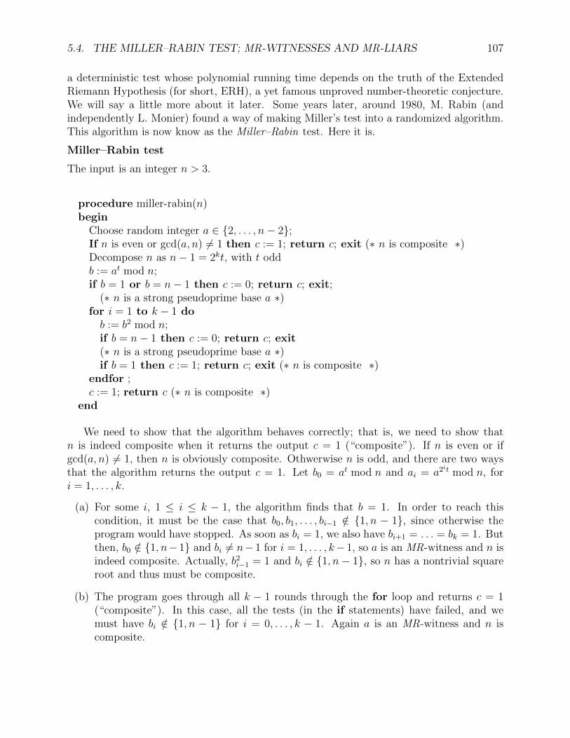
5.4. THE MILLER–RABIN TEST; MR-WITNESSES AND MR-LIARS 107
a deterministic test whose polynomial running time depends on the truth of the ExtendedRiemann Hypothesis (for short, ERH), a yet famous unproved number-theoretic conjecture.We will say a little more about it later. Some years later, around 1980, M. Rabin (andindependently L. Monier) found a way of making Miller’s test into a randomized algorithm.This algorithm is now know as the Miller–Rabin test. Here it is.
Miller–Rabin test
The input is an integer n > 3.
procedure miller-rabin(n)begin
Choose random integer a ∈ 2, . . . , n− 2;If n is even or gcd(a, n) 6= 1 then c := 1; return c; exit (∗ n is composite ∗)Decompose n as n− 1 = 2kt, with t oddb := at mod n;if b = 1 or b = n− 1 then c := 0; return c; exit;
(∗ n is a strong pseudoprime base a ∗)for i = 1 to k − 1 dob := b2 mod n;if b = n− 1 then c := 0; return c; exit(∗ n is a strong pseudoprime base a ∗)if b = 1 then c := 1; return c; exit (∗ n is composite ∗)
endfor ;c := 1; return c (∗ n is composite ∗)
end
We need to show that the algorithm behaves correctly; that is, we need to show thatn is indeed composite when it returns the output c = 1 (“composite”). If n is even or ifgcd(a, n) 6= 1, then n is obviously composite. Othwerwise n is odd, and there are two waysthat the algorithm returns the output c = 1. Let b0 = at mod n and ai = a2
it mod n, fori = 1, . . . , k.
(a) For some i, 1 ≤ i ≤ k − 1, the algorithm finds that b = 1. In order to reach thiscondition, it must be the case that b0, b1, . . . , bi−1 /∈ 1, n − 1, since otherwise theprogram would have stopped. As soon as bi = 1, we also have bi+1 = . . . = bk = 1. Butthen, b0 /∈ 1, n− 1 and bi 6= n− 1 for i = 1, . . . , k− 1, so a is an MR-witness and n isindeed composite. Actually, b2i−1 = 1 and bi /∈ 1, n− 1, so n has a nontrivial squareroot and thus must be composite.
(b) The program goes through all k − 1 rounds through the for loop and returns c = 1(“composite”). In this case, all the tests (in the if statements) have failed, and wemust have bi /∈ 1, n − 1 for i = 0, . . . , k − 1. Again a is an MR-witness and n iscomposite.
108 CHAPTER 5. THE MILLER–RABIN TEST
The computational complexity of this algorithm depends on what kind of fast algorithmis used to compute exponentiation modulo n. As explained in Dietzfelbinger [4] (Chapter 5,Section 5.2), it takes O(log2 n) arithmetic operations and O((log2 n)3) bit operations. If afaster method is used for integer multiplication, then it takes O∼((log2 n)2) bit operations.Here, the notation f = O∼(g) means that f = O(g(log2(g))k), for some k ≥ 0; for details,see Dietzfelbinger [4] (Chapter 2, Sections 2.2 and 2.3). In brief, the Miller–Rabin test ispolynomial in the bit length of the input n (of degree at most 3).
It remains to show that the probability that the Miller–Rabin test gives the wrong answer,“strong pseudoprime,” when n is a composite, is less than 1/2. Monier and Rabin provedthat this probability is actually less than 1/4, but for now, we show that this probability isless than 1/2 because the proof is simpler. We follow the nice proof given in Dietzfelbinger[4] (Chapter 5).
We need to find an upper bound on |LMRn |. As we explained earlier, the set LMR
n ofMR-liars is contained in LFn , but it is not a subgroup.
If n is not a Carmichael number, then LFn is a proper subgroup of (Z/nZ)∗, so the reason-ing used in the proof of Proposition 5.4 applies, and the fraction of MR-liars in 2, . . . , n−2is less than 1/2.
If n is a Carmichael number, then we can find a proper subgroup Bn of (Z/nZ)∗ thatcontains LMR
n as follows. Write n−1 = 2kt, with t odd. Since t is odd, we have (n−1)t ≡ n−1(mod n), so there is a largest index i ≥ 0 such that there is an MR-liar a0 (recall thata0 ∈ 1, . . . , n− 1) with
a2it
0 ≡ n− 1 (mod n).
Denote this largest index by i0. Since n is a Carmichael number, we have
a2kt
0 ≡ an−10 ≡ 1 (mod n),
hence 0 ≤ i0 ≤ k − 1. Define Bn by
Bn = a ∈ 1, . . . , n− 1 | a2i0 t mod n ∈ 1, n− 1.
The following proposition is the key ingredient.
Proposition 5.8. The set Bn defined above (for a Carmichael number n) has the followingproperties:
(1) LMRn ⊆ Bn.
(2) The set Bn is a subgroup of (Z/nZ)∗.
(3) The group Bn is a proper subgroup of (Z/nZ)∗.
5.4. THE MILLER–RABIN TEST; MR-WITNESSES AND MR-LIARS 109
Proof. (1) Pick any a ∈ LMRn .
Case 1: at ≡ 1 (mod n). Then, a2i0 t ≡ 1 (mod n) as well, and thus a ∈ Bn.
Case 2: a2it ≡ n − 1 (mod n), for some i with 0 ≤ i ≤ k − 1. By the maximality of i0,
we have i ≤ i0. If i = i0, then we get immediately that a ∈ Bn. If i < i0, then
a2i0 t ≡
(a2
it mod n)2i0−i
≡ 1 (mod n)
since i0 − i ≥ 1, and we conclude that a ∈ Bn.
(2) Obviously, 1 ∈ Bn. Since (Z/nZ)∗ is finite, we only need to check that Bn is closedunder multiplication. Pick a, b ∈ Bn. This means that a2
i0 t mod n and b2i0 t mod n belong
to 1, n− 1. Now, we have
1 · 1 ≡ 1 (mod n)
1 · (n− 1) ≡ n− 1 (mod n)
(n− 1) · 1 ≡ n− 1 (mod n)
(n− 1) · (n− 1) ≡ 1 (mod n),
which implies that(ab)2
i0 t ≡ a2i0 tb2
i0 t ≡ 1 or n− 1 (mod n);
that is, ab ∈ Bn, as required.
(3) We need to find some a ∈ (Z/nZ)∗ which does not belong to Bn. We use the fact thata Carmichael number can be written as the product n = n1n2 of two distinct odd numbersn1 and n2 such that gcd(n1, n2) = 1, which is a consequence of the fact that a Carmichaelnumber is a product of (at least 3) distinct primes.
Recall that a0 is an MR-liar with a2i0 t
0 ≡ n − 1 (mod n). Since n1 and n2 divide n, wealso have a2
i0 t0 ≡ n− 1 (mod n1) and a2
i0 t0 ≡ n− 1 (mod n2). If we let a1 ≡ a0 mod n1, then
by the Chinese remainder theorem, there is a unique a ∈ 0, . . . , n− 1 such that
a ≡ a1 (mod n1)
a ≡ 1 (mod n2).
We claim that a ∈ (Z/nZ)∗, but a /∈ Bn. First, we show that a /∈ Bn.
From a1 ≡ a0 (mod n1) and a ≡ a1 (mod n1), we get a ≡ a0 (mod n1), and sincea2
i0 t0 ≡ n− 1 (mod n1), we get
a2i0 t ≡ n− 1 (mod n1). (∗)
From a ≡ 1 (mod n2), we get
a2i0 t ≡ 1 (mod n2). (∗∗)
110 CHAPTER 5. THE MILLER–RABIN TEST
Now, since n1 divides n, (∗) implies that
a2i0 t 6≡ 1 (mod n),
and since n2 divides n, (∗∗) implies that
a2i0 t 6≡ n− 1 (mod n).
Consequently, a2i0 t mod n /∈ 1, n − 1, and thus a /∈ Bn. It remains to show that a ∈
(Z/nZ)∗. By squaring (∗) and (∗∗) , we get
a2i0+1t ≡ 1 (mod n1) and a2
i0+1t ≡ 1 (mod n2),
and since gcd(n1, n2) = 1, this yields
a2i0+1t ≡ 1 (mod n),
which shows that a ∈ (Z/nZ)∗ (by Proposition 5.3).
Proposition 5.8 shows that if n is a Carmichael number, then LMRn is contained in the
proper subgroup Bn of (Z/nZ)∗, and by the reasoning used when LMRn is contained in the
proper subgroup LFn of (Z/nZ)∗, we conclude that the fraction of MR-liars in 2, . . . , n− 2is also less than 1/2. In summary, we proved the following result.
Theorem 5.9. If n > 3 is an odd composite, then the fraction of MR-liars in 2, . . . , n− 2is less than 1/2. Consequently, the probability that the Miller–Rabin test gives the wronganswer c = 0, more precisely the probability that any a ∈ 2, . . . , n− 2 is a MR-liar, is lessthan 1/2.
We will show below that if we repeat the Miller–Rabin test ` times, then the probabilitythat the algorithm gives the answer c = 0 every time when n is composite is at most (1/2)`.Here is the algorithm.
Algorithm Probable Prime
The input is an integer n > 3.
beginfor i = 1 to ` doc = miller-rabin(n);if c = 1 then res = 1; return res; exit (∗ n is composite ∗)
endfor ;res = 0; return res (∗ n is a probable prime ∗)
end
5.4. THE MILLER–RABIN TEST; MR-WITNESSES AND MR-LIARS 111
We can easily modify miller-rabin to avoid redecomposing n again and again when it iscalled.
If the algorithm stops with res = 1, then n is definitely composite. If n is prime, thenthe algorithm will runs through all ` steps and correctly return res = 0. If n is composite,the algorithm may return the wrong answer res = 0, but the probability that this happensis bounded by (1/2)`.
We hinted earlier at the fact that the above probabilily is not really what we would liketo know. To make this point clearer, let us define the events P,C, SP and SP ` by
P = n | n ≥ 3, n is primeC = n | n ≥ 3, n is composite
SP = n | n ≥ 3, the miller-rabin procedure returns c = 0SP ` = n | n ≥ 3, the miller-rabin procedure returns c = 0 ` times.
Observe that P = C, the complement of C. Then, we have the three conditional probabilities
Pr(P | SP `) = Pr(n is not composite | miller-rabin returns c = 0 ` times)
= Pr(n is prime | miller-rabin returns c = 0 ` times),
Pr(SP ` | P ) = Pr(miller-rabin returns c = 0 ` times | n is not composite)
= Pr(miller-rabin returns c = 0 ` times | n is prime)
andPr(SP ` | C) = Pr(miller-rabin returns c = 0 ` times | n is composite).
The third probability Pr(SP ` | C) is the one we have been considering so far, but we shouldbe more interested in the level of confidence that n is prime given that miller-rabin returnsres = 0, and this is the first probability Pr(P | SP `). This point is clearly articulated inHoffstein, Pipher and Silverman [8]; most of the literature ignores it, and it is important tomake it perfectly clear. Fortunately, Pr(P | SP `) can be obtained using Bayes’s formula:
Pr(P | SP `) =Pr(SP ` | P )Pr(P )
Pr(SP ` | P )Pr(P ) + Pr(SP ` | P )Pr(P ).
In particular, we need to compute the probability Pr(P ) that an integer n ≥ 3 is prime. Butthere is a problem: the events under consideration are all infinite, so their probabilities arenot well defined! A positive integer either is prime or is not prime; it cannot be 30% primeand 70% composite.
The problem with infinite events is pointed out by Hoffstein, Pipher and Silverman in[8] (Chapter 3, Section 3.4.1). The statement often found that a randomly chosen positiveinteger has probability 1/ lnn of being prime is meaningless. In order for all these probabil-ities to make sense, we need our events to be finite, and this can be achieved if we considerfinite intervals.

112 CHAPTER 5. THE MILLER–RABIN TEST
We can make this idea precise following the hint given in Exercise 3.18 in Hoffstein,Pipher and Silverman in [8].
Let c1 < c2 be any two positive real numbers. For any positive integer n, let us find theprobabilty P (c1, c2;n) that an integer m such that c1n ≤ m ≤ c2n is prime,
P (c1, c2;n) = Pr(m is prime, c1n ≤ m ≤ c2n).
The condition c1n ≤ m ≤ c2n is really dc1ne ≤ m ≤ bc2nc. Since c1 < c2, there are bc2nc −dc1ne+1 ≈ (c2−c2)n integers in the interval [dc1ne, bc2nc]. There are π(bc2nc)−π(dc1ne−1)primes in the interval [dc1ne, bc2nc], which by the Prime Number Theorem is approximately
π(bc2nc)− π(dc1ne − 1) ≈ c2n
ln(c1n)− c1n
ln(c1n)
=n(c2 ln(c1n)− c1 ln(c2n))
ln(c1n) ln(c2n)
=n((c2 − c1) lnn+ c2 ln c1 − c1 ln c2)
(lnn+ ln c1)(lnn+ ln c2).
Consequently, the probability P (c1, c2;n) given by
P (c1, c2;n) =π(bc2nc)− π(dc1ne − 1)
bc2nc − dc1ne+ 1
is approximately
P (c1, c2;n) =
(1 +
c2 ln(c1)− c1 ln(c2)
(c2 − c1) lnn
)lnn
(1 +
ln c1lnn
)(1 +
ln c2lnn
) .When n is large, this probability is approximately
P (c1, c2;n) =1
lnn,
independently of c1 and c2.
The above derivation justifies saying that for n large enough, the probability that aninteger m in an interval [dc1ne, bc2nc] is prime is approximately 1/ lnn.
We can choose c1 and c2 so that 0 < c1 < 1 and c2 > 1 (for example, c1 = 12, c2 = 3
2) so
that c1n ≤ n ≤ c2n , and as long as n is large enough so that
c2 ln(c1)− c1 ln(c2)
(c2 − c1) lnn,
ln c1lnn
, andln c2lnn
are very close to 0, the probability that some m ∈ [dc1ne, bc2nc] is prime is approximately1
lnn.

5.4. THE MILLER–RABIN TEST; MR-WITNESSES AND MR-LIARS 113
In view of all this, we revise the definitions of our events P,C, SP and SP ` as follows.We pick some real numbers c1 and c2 such that 0 < c1 < 1 and c2 > 1; for example, c1 = 1
2
and c2 = 32. For any positive integer n, let I(c1, c2;n) be the interval
I(c1, c2;n) = m ∈ N | dc1ne ≤ m ≤ bc2nc].
We may assume that n is large enough and that c1 is chosen so that dc1ne ≥ 3. For example,c1 = 1
2and n ≥ 6 will do. Then we define the following events:
P (c1, c2;n) = m | m ∈ I(c1, c2;n), m is primeC(c1, c2;n) = m | m ∈ I(c1, c2;n), m is composite
SP(c1, c2;n) = m | m ∈ I(c1, c2;n), the miller-rabin procedure returns c = 0SP `(c1, c2;n) = m | m ∈ I(c1, c2;n), the miller-rabin procedure returns c = 0 ` times,
To simplify notation, we write P (n), C(n), SP(n), SP `(n) instead of P (c1, c2;n), C(c1, c2;n),SP(c1, c2;n), SP `(c1, c2;n), and we also write I(n) instead of I(c1, c2;n). Then we definethe three conditional probabilities
Pr(P (n) | SP `(n)) = Pr(m ∈ I(n) is prime | miller-rabin returns c = 0 ` times),
Pr(SP `(n) | P (n)) = Pr(miller-rabin returns c = 0 ` times | m ∈ I(n) is prime)
and
Pr(SP `(n) | C(n)) = Pr(miller-rabin returns c = 0 ` times | m ∈ I(n) is composite).
To compute the probabilities on the righthand side, we use the fact that our Miller–Rabinalgorithm (the procedure miller-rabin, not the algorithm Probable Prime) is a Monte Carloalgorithm, which means the following:
(1) If miller-rabin returns c = 1, then m ∈ I(n) definitely is composite (i.e. has PropertyC(n)). This is expressed by
Pr(m ∈ I(n) is composite | miller-rabin returns c = 1) = 1,
or more concisely asPr(C(n) | SP(n)) = 1.
(2) If m ∈ I(n) is composite (has property C(n)), then miller-rabin returns c = 1 for atleast 1/2 of the number of choices for a. This is expressed by
Pr(miller-rabin returns c = 1 | m ∈ I(n) is composite) ≥ 1
2,
or more concisely as
Pr(SP(n) | C(n)) ≥ 1
2.

114 CHAPTER 5. THE MILLER–RABIN TEST
From Property (1) of a Monte Carlo algorithm, by contrapositive, we see that if m is notcomposite, then the algorithm always returns c = 0; that is,
Pr(miller-rabin returns c = 0 | m ∈ I(n) is prime) = 1,
or more concisely asPr(SP(n) | P (n)) = 1.
It follows thatPr(SP `(n) | P (n)) = Pr(SP(n) | P (n))` = 1.
To evaluate Pr(SP ` | P (n)) = Pr(SP ` | C(n)) we make use of the assumption that miller-rabin is run ` independent times and that by Property (2) of a Monte Carlo algorithm,
Pr(SP(n) | C(n)) ≥ 1
2,
so we have
Pr(SP `(n) | C(n)) = Pr(SP(n) | C(n))`
= (1− Pr(SP(n) | C(n)))`
≤(
1− 1
2
)`=
(1
2
)`.
The above derivation shows rigorously what we have been claiming: the probability that thealgorithm says ` times that m ∈ I(n) is not a composite when in fact it is, is very small.Indeed,
Pr(SP `(n) | C(n)) ≤(
1
2
)`.
As we said earlier, the probability we really want to know is Pr(P (n) | SP `(n)). We have allthe ingredients to compute it, since we showed earlier that Pr(P (n)) is approximately
Pr(P (n)) =1
lnn.
Then we compute Pr(P (n) | SP `) using Bayes’rule, and we have
Pr(P (n) | SP `(n)) =Pr(SP `(n) | P (n))Pr(P (n))
Pr(SP `(n) | P (n))Pr(P (n)) + Pr(SP `(n) | P (n))Pr(P (n))
≥1 · 1
ln(n)
1 · 1ln(n)
+ 2−`(
1− 1ln(n)
)=
1
1 + 2−`(ln(n)− 1)
= 1− ln(n)− 1
2` + ln(n)− 1> 1− ln(n)
2`.
5.4. THE MILLER–RABIN TEST; MR-WITNESSES AND MR-LIARS 115
Therefore, if ` is large enough so that 2` > ln(n)
Pr(P (n) | SP `(n)) > 1− ln(n)
2`,
(approximately), and we see that it is necessary to add a correction term approximatelyequal to ln(n), but this correction term is quickly offset by making ` a little bigger.
Our Monte Carlo algorithm does not give a definite answer. However, if ` is large enough,say ` = 100, then the conditional probability that the number being tested is prime giventhat the test is negative ` times, is very close to 1 (note that 2−100 < 10−30). In other words,the degree of confidence that the number being tested is prime is very high.
Actually, Rabin and Monier independently proved in 1980 that if m is composite thenthe Miller–Rabin procedure returns c = 1 for at least 3/4 of the number of choices for a(provided that m > 9); this implies that
Pr(SP(n) | C(n)) ≥ 3
4.
Therefore, Pr(SP(n) | C(n)) ≤ 1/4, and for ` large enough, we have
Pr(P (n) | SP `(n)) > 1− ln(n)
4`.
This shows that the Miller–Rabin procedure provides a higher degree of confidence thanwe originally found, in the sense that if the test is negative ` times for ` large enough, say` = 100, then Pr(P (n) | SP `(n)) is much closer to 1 than we originally determined.
For example, since (1/4)100 < 2−60 and since ln(10) ≈ 2.303, for n = 101020 (a very largenumber with 1020 digits), we have
Pr(P (n) | SP100(n)) > 1− ln(n)
4`> 1− 2.31 · 1020 · 10−60 > 1− 10−39.
This is a very small probability.
In order to prove that Pr(SP(n) | C(n)) ≤ 1/4, Rabin and Monier proved that if n > 9is an odd composite, then
|LMRn | ≤
ϕ(n)
4.
The proof is harder than the proof of Proposition 5.8, but it is not out of reach given a littlebit of number theory. The general strategy is also to find a proper subgroup of (Z/nZ)∗ thatcontains LMR
n and to estimate its order, to show that it is bounded by ϕ(n)/4. The proofgiven in Crandall and Pomerance [3] (Chapter 3, Section 5) is presented in the next section.This proof mixes combinatorial and number theoretic ideas in a beautiful and clever way,but it can be omitted without causing a major gap in the understanding of the Miller–Rabintest. The probability Pr(SP(n) | C(n)) ≤ 1/2 is good enough to prove that the Miller–Rabintest can be trusted with a high degree of confidence.

116 CHAPTER 5. THE MILLER–RABIN TEST
5.5 The Monier–Rabin Bound on the Size of the Set
of MR-liars
Let n ≥ 2 be any odd integer and suppose that its prime factorization is
n = pj11 pj22 · · · p
jkk , ji ≥ 1, i = 1, . . . , k.
Since n is odd, all the pi are odd. Write ω(n) = k for the number of distinct prime factorsin n. The key point is that LMR
n is a subset of a group S(n) of the form
S(n) = a ∈ (Z/nZ)∗ | am ≡ ±1 (mod n),
for some suitable m (depending on n), such that m divides n − 1. Thus, to estimate theorder of this group, we need to find the number of solutions a (mod n) to the congruence
am ≡ ±1 (mod n).
We will see that the second congruence (the case −1) reduces to the first (the case +1), so weare reduced to the problem of counting the number of solutions a (mod n) to the congruence
am ≡ 1 (mod n). (∗)
This is where some number theory comes in handy. Firstly, since the pjii are relatively prime,a ∈ Z is a solution of (∗) iff a is a solution of the k congruences
am ≡ 1 (mod pjii ), i = 1, . . . , k. (∗∗)
Now, because pi is an odd prime, the group of units (Z/pjii Z)∗ of the ring Z/pjii Z is cyclic(see Theorem 4.42). This means that there is some g ∈ (Z/pjii Z)∗ (called a primitive rootmodulo pjii ) such that
g, g2, . . . , gϕ(pjii )−1, gϕ(p
jii ) = 1
is a list of all elements in (Z/pjii Z)∗. Then, we can easily determine when an elementa ∈ (Z/pjii Z)∗ is a solution of
am ≡ 1 (mod pjii ). (†)
If we write a = gk, for some k with 1 ≤ k ≤ ϕ(pjii ), then we must have
gkm ≡ 1 (mod pjii ).
Now, g ∈ (Z/pjii Z)∗ has order ϕ(pjii ) (the smallest integer r such that gr ≡ 1 (mod pjii )), soϕ(pjii ) must divide km. If d = gcd(m,ϕ(pjii )) and if we write m = dm1 and ϕ(pjii ) = dn1,then gcd(m1, n1) = 1 and ϕ(pjii ) must divide km iff n1 divides km1. Since gcd(m1, n1) = 1,the number n1 must divide k, and we find d solutions for k:
n1, 2n1, . . . , (d− 1)n1, dn1 = ϕ(pjii ).

5.5. THE MONIER–RABIN BOUND ON THE SIZE OF THE SET OF MR-LIARS 117
Therefore, we proved that equation (†) has
gcd(m,ϕ(pjii ))
solutions modulo pjii . Since m divides n − 1, it is not divisible by pi (because pi divides nand pi ≥ 3), and since ϕ(pjii ) = pjii (pi − 1), we get
gcd(m,ϕ(pjii )) = gcd(m, pjii (pi − 1)) = gcd(m, pi − 1).
By the Chinese remainder theorem, the solutions of (∗) modulo n are in bijection with thek-tuples (a1, . . . , ak), where each ai is a solution of (†) modulo pjii . It follows that the numberof solutions modulo n of the congruence am ≡ 1 (mod n) is
k∏i=1
gcd(m, pi − 1).
In summary, we proved the following result.
Proposition 5.10. Let n ≥ 2 be any odd integer and suppose that its prime factorization is
n = pj11 pj22 · · · p
jkk , ji ≥ 1, i = 1, . . . , k.
For any integer m ≥ 1 such that m divides n − 1, the number of solutions modulo n of thecongruence
am ≡ 1 (mod n)
isk∏i=1
gcd(m, pi − 1).
An interesting corollary of Proposition 5.10 obtained by setting m = n− 1 is that everyodd composite number n is a pseudoprime for at least two nontrivial bases a 6= ±1 modulon, unless n is a power of 3.
We now return to the definition of the group S(n).
Definition 5.6. For any odd composite n, if n − 1 = 2st, with t odd, then let ν(n) be thelargest integer such that 2ν(n) divides p− 1 for every prime factor p of n. Then let
S(n) = a ∈ (Z/nZ)∗ | a2ν(n)−1t ≡ ±1 (mod n).
The following proposition shows why S(n) is relevant.
Proposition 5.11. For any odd composite integer n, the following properties hold:
(1) The set of MR-liars LMRn is contained in S(n).

118 CHAPTER 5. THE MILLER–RABIN TEST
(2) The set S(n) is a subgroup of (Z/nZ)∗.
Proof. (1) Pick any a ∈ LMRn . There are two cases.
(i) If at ≡ 1 (mod n), then obviously a2ν(n)−1t ≡ 1 (mod n), so a ∈ S(n).
(ii) There is some smallest index i with 0 ≤ i ≤ s − 1 such that a2it ≡ n − 1 ≡ −1
(mod n). For any prime p dividing n, we also have a2it ≡ −1 (mod p), and so
a2i+1t ≡ 1 (mod p).
If k is the order of a in (Z/pZ)∗, then k divides 2i+1t but k does not divide 2it. This isbecause if k divides 2it, then we can write 2it = kq, and then
a2it ≡ akq ≡ (ak)q ≡ 1q ≡ 1 (mod p)
since ak ≡ 1 (mod p) as k is the order of a modulo p, contradicting a2it ≡ −1 (mod p).
It follows that 2i+1 is the exact power of 2 in the prime factorization of k so we can writek = 2i+1t1 for some t1. Since by Fermat’s little theorem, ap−1 ≡ 1 (mod p), we see thatk = 2i+1t1 divides p−1, and so 2i+1 divides p−1. Since this holds for every prime p dividingn, we have i + 1 ≤ ν(n). Since a2
it ≡ −1 (mod n), if i + 1 < ν(n), then by squaring we
obtain a2i+1t ≡ 1 (mod n), so a2
ν(n)−1t ≡ 1 (mod n), else if i+ 1 = ν(n), then a2ν(n)−1t ≡ −1
(mod n). In both cases, a ∈ S(n).
(2) The proof that S(n) is a group is very similar to the fact that Bn is a group (see theproof of Proposition 5.8) and is left an an exercise.
The next proposition gives a formula for the order of the group S(n).
Proposition 5.12. For any odd composite integer n, if we denote the number of distinctprime factors of n by ω(n) and if n − 1 = 2st with s, t and ν(n) as in Definition 5.6, thenthe order of the group S(n) is given by
|S(n)| = 2 · 2(ν(n)−1)ω(n)∏p|n
gcd(t, p− 1).
Proof. Since
S(n) = a ∈ Z/nZ | a2ν(n)−1t ≡ ±1 (mod n),
we need to count the number s1 of solutions of the congruence a2ν(n)−1t ≡ 1 (mod n) and
the number s2 of solutions of a2ν(n)−1t ≡ −1 (mod n). As to the first congruence, if we let
m = 2ν(n)−1t, by definition of ν(n), we know that 2ν(n) divides p−1 for every prime p dividingn. Let n = pj11 · · · p
jkk be a prime factorization of n, where p1, . . . , pk are the distinct prime
factors of n (with k = ω(n)), which must be odd since n is odd. We have pi− 1 = 2ν(n)ti forsome ti. If we had ν(n) > s, then since
pi − 1 = 2ν(n)ti = 2s+12ν(n)−s−1ti
5.5. THE MONIER–RABIN BOUND ON THE SIZE OF THE SET OF MR-LIARS 119
we could write pi = 1 + 2s+1ui for some integers ui = 2ν(n)−s−1ti, and then n− 1 = 2st wouldyield
(2s+1u1 + 1) · · · (2s+1uk + 1)− 1 = 2st,
which would imply that2s+1u = 2st,
for some integer u. Since t is odd, this is impossible, and thus ν(n) ≤ s. Consequently,m = 2ν(n)−1t divides n− 1 = 2st. By Proposition 5.10, we have
s1 =
ω(n)∏i=1
gcd(m, pi − 1).
But m = 2ν(n)−1t, t is odd and 2ν(n) divides each pi − 1, so
gcd(m, pi − 1) = gcd(2ν(n)−1t, pi − 1) = 2ν(n)−1gcd(t, pi − 1),
so we get
s1 = 2(ν(n)−1)ω(n)ω(n)∏i=1
gcd(t, pi − 1).
We now show that because n is odd the congruence am ≡ −1 (mod n) has the same numberof solutions as the congruence am ≡ 1 (mod n).
For every odd prime pi as above, we claim that am ≡ −1 (mod pjii ) iff a2m ≡ 1 (mod pjii )and am 6≡ 1 (mod pjii ).3 Obviously, if am ≡ −1 (mod pjii ), then (am)2 ≡ a2m ≡ 1 (mod pjii )and am 6≡ 1 (mod pjii ). Conversely, by Proposition 5.1, if pi is an odd prime then thereare exactly two square roots of unity mod pjii , namely +1 and −1. So if (am)2 ≡ a2m ≡ 1(mod pjii ), then either am ≡ 1 (mod pjii ) or am ≡ −1 (mod pjii ), but since am 6≡ 1 (mod pjii ),we mut have am ≡ −1 (mod pjii ).
We observed earlier that 2ν(n) divides pi − 1, and it follows as above that the number ofsolutions of the equation am ≡ −1 (mod pjii ) is
2ν(n)gcd(t, pi − 1)− 2ν(n)−1gcd(t, pi − 1) = 2ν(n)−1gcd(t, pi − 1).
It follows that the number s2 of solutions of am ≡ −1 (mod n) is
s2 = s1.
Therefore, the order of the group S(n) is indeed
|S(n)| = 2 · 2(ν(n)−1)ω(n)∏p|n
gcd(t, p− 1),
as claimed.3I thank Tian Bai for pointing out an error in my previous proof, which claimed that the above fact held
for any n rather that for each pjii with pi an odd prime.
120 CHAPTER 5. THE MILLER–RABIN TEST
Proposition 5.12 yields the main result of this section.
Theorem 5.13. (Monier–Rabin) For every odd composite n > 9, we have
|LMRn | ≤
ϕ(n)
4≤ n− 1
4.
Proof. As usual, write n − 1 = 2st, with t odd. By Proposition 5.11, LMRn ⊆ S(n), so it
suffices to prove that |S(n)|/ϕ(n) ≤ 14. If n = pj11 p
j22 · · · p
jkk is the prime factorization of n,
recall thatϕ(n) = pj1−11 (p1 − 1)pj2−12 (p2 − 1) · · · pjk−1k (pk − 1).
By Proposition 5.12,
|S(n)| = 2 · 2(ν(n)−1)ω(n)∏p|n
gcd(t, p− 1),
so we need to prove that
ϕ(n)
|S(n)|=
1
2
∏pk‖n
pk−1p− 1
2ν(n)−1gcd(t, p− 1)≥ 4,
where the notation pk‖n means that pk is the exact power of the prime p in the primefactorization of n. Each factor
p− 1
2ν(n)−1gcd(t, p− 1)(∗)
is an even integer. There are several cases.
Case 1: ω(n) ≥ 3. In this case, at least three of the factors (∗) are equal to 2, soϕ(n)/|S(n)| ≥ 4.
Case 2: ω(n) = 2 and n is not squarefree. Then, some exponent k − 1 is at least 1, andsince all the primes p are odd, the product of the pk−1 is at least 3, each factor (∗) is at least2, so ϕ(n)/|S(n)| ≥ 6.
Case 3: n = pq, for two distinct primes, p, q, with p < q. If 2ν(n)+1 divides q − 1, thenq − 1 = 2ν(n)+1u, and t is odd, we get
2ν(n)−1gcd(t, q − 1) = 2ν(n)−1gcd(t, 2ν(n)+1u) = 2ν(n)−1gcd(t, u) ≤ 2ν(n)−1u = (q − 1)/4,
and since the other fraction involving p− 1 is at least 2, we get ϕ(n)/|S(n)| ≥ 4.
The remaining subcase is that 2ν(n) is the exact power of 2 in q − 1, and we can writeq− 1 = 2ν(n)u, where u is odd. Because n− 1 = pq− 1 = p(q− 1) + p− 1 and p < q, we seethat q− 1 does not divide n− 1. This implies that there is an odd prime q1 dividing q− 1 toa higher power than it divides n− 1. Since n− 1 = 2st and q − 1 = 2ν(n)u, we have t = qh1 t1and u = qh+1
1 u1 for some h ≥ 1 and some t1, u1 with gcd(q1, t1) = 1. It follows that
q − 1 = 2ν(n)qh+11 u1

5.6. THE LEAST MR-WITNESS FOR n 121
and
2ν(n)−1gcd(t, q − 1) = 2ν(n)−1gcd(qh1 t1, 2ν(n)qh+1
1 u1)
= 2ν(n)−1qh1gcd(t1, q1u1)
= 2ν(n)−1qh1gcd(t1, u1)
≤ 2ν(n)−1qh1u1
=(q − 1)
2q1≤ q − 1
6.
Since the other fraction is at least 2, we conclude that ϕ(n)/|S(n)| ≥ 6.
Case 4: n = pk, for some k ≥ 2. In this case, n − 1 = pk − 1 = 2st with t odd. Sincek ≥ 2, we have
pk − 1 = (p− 1)(pk−1 + · · ·+ p+ 1) = 2st,
and sincep− 1 = 2ν(n)u
with u odd, we conclude that u is a divisor of t. Then
gcd(t, p− 1) = gcd(t, 2ν(n)u) = gcd(t, u) = u,
which implies thatp− 1
2ν(n)−1gcd(t, p− 1)=
2ν(n)u
2ν(n)−1u= 2,
and thus, ϕ(n)/|S(n)| = pk−1. Therefore, unless pk = 9, which means that k = 2 and p = 3,we have ϕ(n)/|S(n)| ≥ 5 (since 5 is the next prime after 3). This last case finishes theproof.
Remarks:
1. Another proof of Theorem 5.13 is given in Koblitz [10] (Chapter V, Proposition V.1.7).
2. The group S(n) is actually the group generated by the set LMRn of MR-liars. This
result due to Jim Haglund is Problem 3.16 in Crandall and Pomerance [3].
5.6 The Least MR-Witness for n
Theorem 5.13 shows that an odd composite n has at least 3n/4 MR-witnesses in the set2, . . . , n− 2. A natural question then arises: what is the size of the smallest MR-witness,W (n), for n? If, by luck, the size of W (n) is bounded by a constant, or a slow-growing func-tion, then there is hope that a practical deterministic algorithm (that is, not a randomizedalgorithm) can be found.
122 CHAPTER 5. THE MILLER–RABIN TEST
Unfortunately, there is no constant bound. Indeed, Alford, Granville and Pomeranceshowed that for infinitely many odd composite n, we have
W (n) > (lnn)1/(3 ln ln lnn).
In Crandall and Pomerance [3], it is also shown that W (n) ≥ 3 for infinitely many n (with anexplicit description). Around 1976, Gary Miller showed that W (n) = O((lnn)2), assumingthat the Extended Riemann Hypothesis (for short ERH) holds. Then, Bach (1985) provedthat W (n) < 2(lnn)2; see Crandall and Pomerance [3] (Chapter 3, Section 3.5).
The ERH is a generalization of the Riemann Hypothesis (for short RH), one of the mostfamous conjectures of mathematics. Explaining what is the ERH would lead us to far, andwe refer the reader to Crandall and Pomerance for an explanation [3] (Chapter 1, Section1.4). However, we discuss briefly the RH.
The RH has to with the location of the zeros of the zeta function, ζ. For any real s > 1,the function ζ(s) is given by
ζ(s) =∞∑n=1
1
ns.
If we allow s to be a complex argument, then the above sum converges absolutely for Re(s) >1. It is also possible to extend ζ to the entire complex plane (by analytic continuation), sothat ζ(s) is regular for every s except s = 1, where it has a simple pole with residue 1 (thismeans that (s − 1)ζ(s) is holomorphic in C, with value 1 at s = 1). Two good sources areApostol [1] and Edwards [5]. Ribenboim’s lovely book [18] (especially Chapter 4) is alsohighly recommended. The connection with prime numbers was noticed by Euler and is this:
Theorem 5.14. (Euler) If P denotes the set of all primes, then for every s ∈ C such thatRe(s) > 1,
ζ(s) =∏p∈P
1
1− p−s.
The value ζ(s) of the zeta-function is known when s is an even integer, but ζ(s) is notknown for not a single odd integer! Remarkably, the location of the zeros of ζ has crucialimpact on the distribution of the primes. For example, the fact that ζ(s) 6= 0 on the lineRe(s) = 1 leads to the Prime Number Theorem. The Riemann Hypothesis, stated in 1859by Riemann in an eight-page memoir, says this:
Conjecture (Riemann hypothesis (RH))
All the zeros of ζ in the critical strip 0 < Re(s) < 1 lie on the vertical line Re(s) = 1/2.
The RH has been verified by computer calculations for many values of n, but it stillremains one of the central conjectures of mathematics. It is equivalent to various statementsabout the distribution of the primes. For example, von Koch proved in 1901 that the RH isequivalent to the following fact:
|π(x)− Li(x)| <√x · ln(x), for all x ≥ 2.01,

5.6. THE LEAST MR-WITNESS FOR n 123
where π(x) is the number of primes not exceeding x, and the function Li (logarithmic integral)is given by
Li(x) =
∫ x
2
dt
ln t.
It is easy to see that
Li(x) =x
lnx+
∫ x
2
dt
(ln t)2− 2
ln 2.
It is amazing that Gauss conjectured in 1791 (at the age of fourteen) that π(x) ∼ Li(x). Werefer the reader to Crandall and Pomerance [3] (Chapter 1) for more on this topic.
The Extended Riemann Hypothesis (ERH) has to do with the zeros of the Dirichlet L-functions L(s, χ), which generalizes the ζ-function. Here, χ denotes a Dirichlet character.Apostol [1] is an excellent source to learn about L-functions. The ζ-function corresponds tothe special case χ = 1. The ERH says this:
Conjecture (Extended Riemann hypothesis (ERH))
For any Dirichlet character χ, all the zeros of L(s, χ) in the region Re(s) > 0 lie on thevertical line Re(s) = 1/2.
Assuming the ERH, Bach’s result, that W (n) < 2(ln)2, yields a deterministic algorithmfor testing for primality. Simply try the Miller–Rabin procedure for a = 2, 3, . . . , 2(lnn)2.Besides the fact that the ERH is still not proved, in practice, the randomized version ofthe Miller–Rabin test is faster. As of now, if you want a reliable test, either you have tohave faith in the ERH, or faith that an event that has probability less than 10−30 will neverhappen in our lifetime. This probability is much smaller than the probability of hardwareor software failure anyway!

124 CHAPTER 5. THE MILLER–RABIN TEST
Chapter 6
The Solovay–Strassen Test
6.1 Quadratic Residues
The Solovay–Strassen primality test was published in 1977, and thus slightly predates theMiller–Rabin test. It is also a randomized algorithm of Monte Carlo type, and it gives theoutput “composite,” given that the input n is composite, with probability greater than 1/2.The Solovay–Strassen is based on a criterion due to Euler to test whether a number whichis not a multiple of a prime p is a quadratic residue. This test involves the Jacobi symbol,which is a generalization of the Legendre symbol. Properties of the Jacobi symbol yield afast method for checking Euler’s criterion.
If p is a prime and m is an integer which is not a multiple of p, we can look for solutionsx of the quadratic congruence
x2 ≡ m (mod p). (∗)In other words, we are looking for a square root of m modulo p.
When p = 2, every odd integer is a quadratic residue and there are no quadratic non-residues. This case is not very interesting, so from now on we assume that p ≥ 3.
If p is an odd prime, note that the above congruence has at most two solutions. Indeed,Z/pZ is a field, so the polynomial x2−m has at most two roots. Moreover, if x is a solutionof (∗), then so is −x, hence the number of solutions is either 0 or 2.
It is convenient to allow p to be any integer ≥ 3.
Definition 6.1. Given any integer n ≥ 3, for any integer m such that gcd(m,n) = 1, wesay that m is a quadratic residue mod n (or a square mod n) if the congruence
x2 ≡ m (mod n) (†)
has a solution. If (†) has no solution we say that m is a quadratic nonresidue mod n.
Observe that the integers m such that gcd(m,n) > 1 are considered neither quadraticresidues nor quadratic nonresidues.
125

126 CHAPTER 6. THE SOLOVAY–STRASSEN TEST
Consider the example n = 13. The squares modulo 13 of the numbers in 1, 2, . . . , 12are
1, 4, 9, 3, 12, 10, 10, 12, 3, 9, 4, 1,
and thus, there are 6 = 12/2 quadratic residues:
1, 3, 4, 9, 10, 12.
The square roots of 12 modulo 13 are 5 and 8. For n = 26, the quadratic residues are
1, 3, 9, 17, 23, 25.
Because 26 is even, they must be odd. For n = 27, the quadratic residues are
1, 4, 7, 10, 13, 16, 19, 22, 25.
When n is prime, as in the case n = 13, there is the same number of quadratic residuesand nonresidues. This is a general fact.
Proposition 6.1. Let p be an odd prime. Then the set of quadratic residues is a subgroup of(Z/pZ)∗ of order (p− 1)/2. This subgroup consists of the residues modulo p of the numbers
12, 22, 32, . . . ,
(p− 1
2
)2
.
Proof. It is clear that 1 is a quadratic residue. If x2 ≡ a (mod p) and y2 ≡ b (mod p), then
(xy)2 ≡ x2y2 ≡ ab (mod p),
so ab is also a quadratic residue, and the quadratic residues form a group.
If x2 ≡ y2 (mod p), then
(x− y)(x+ y) ≡ 0 (mod p).
Assume that 1 ≤ x, y ≤ (p− 1)/2. Since p is prime, either p divides x− y or p divides x+ y.But, 1 ≤ x, y ≤ (p − 1)/2, which implies 2 ≤ x + y ≤ p − 1, so x − y must be divisible byp, and thus x = y. Therefore, the residues modulo p of the square numbers listed in theproposition are all distinct. Since
(p− k)2 ≡ k2 (mod p),
every quadratic residue modulo p is congruent to a unique number in this list.

6.2. THE LEGENDRE SYMBOL 127
When p is an odd prime, we know that (Z/pZ)∗ is cyclic (see Theorem 4.34). If g is anyprimitive root for (Z/pZ)∗, then gp−1 ≡ 1 (mod p), so
(g(p−1)/2)2 ≡ gp−1 ≡ 1 (mod p),
and g(p−1)/2 is a square root of 1. Since Z/pZ is a field, the only square roots of 1 are ±1,so g(p−1)/2 ≡ ±1 (mod p). But if g(p−1)/2 ≡ 1 (mod p) then g is not a primitive root, sog(p−1)/2 ≡ −1 (mod p).
Proposition 6.1 also shows the following fact.
Proposition 6.2. If p is an odd prime, then for any primitive root g ∈ (Z/pZ)∗, thequadratic residues are the even powers g2i, and the quadratic nonresidues are the odd powersg2i+1, with 0 ≤ i ≤ (p− 3)/2.
We can use the above fact to find square roots modulo p for primes of the form p = 4k+3.Indeed, if a = g2i is any quadratic residue, then we claim that
x = a(p+1)/4 = ak+1
is a square root of a modulo p.
Since g(p−1)/2 ≡ −1 (mod p), we get
x ≡ a(p+1)/4 ≡ (g2i)(p+1)/4 ≡ gi(p+1)/2 ≡ gi(p−1)/2gi ≡ (g(p−1)/2)igi ≡ (−1)igi (mod p),
and thus,x2 ≡ (−1)2ig2i ≡ a (mod p).
If p is a prime of the form p = 4k+ 1, it is (a lot!) harder to find square roots modulo p; seethe end of Section 6.5, and Crandall and Pomerance [3] (Chapter 2, Section 3).
6.2 The Legendre Symbol
At this stage, it is convenient to introduce the Legendre symbol. The remarkable fact aboutthe Legendre symbol is that it gives us an efficient method for testing whether a number mis a quadratic residue mod n without actually solving the congruence x2 ≡ m (mod n). TheJacobi symbol defined in Section 6.3 gives us an even more efficient method which avoidsfactoring.
Definition 6.2. Let p be an odd prime. For any integer m, the Legendre symbol(mp
)is
defined as follows:
(m
p
)=
+1 if m is a quadratic residue modulo p
−1 if m is a quadratic nonresidue modulo p
0 if p divides m.
128 CHAPTER 6. THE SOLOVAY–STRASSEN TEST
Observe that(1p
)= 1 and
(m2
p
)= 1 for every integer m which is not a multiple of p. For
a numerical example, since the squares modulo 11 of the numbers in 1, 2, . . . , 10 are
1, 4, 9, 5, 3, 3, 5, 9, 4, 1,
we see that 7 is not a quadratic residue modulo 11, so(
711
)= −1. We saw earlier that the
quadratic residues modulo 13 are 1, 3, 4, 9, 10, 1 so(
313
)= 1.
If m ≡ n (mod p), then clearly(mp
)=(np
), so the function m 7→
(mp
)is periodic with
period p. We also have (mn
p
)=
(m
p
)(n
p
),
a very useful property for evaluating the Legendre symbol. To prove this property easily, wewill establish Euler’s criterion. First, observe that for any m which is not a multiple of p,by Fermat’s little theorem, we have
mp−1 ≡ 1 (mod p).
If p is an odd prime, then we get
mp−1 − 1 ≡ (m(p−1)/2 − 1)(m(p−1)/2 + 1) ≡ 0 (mod p),
and it follows thatm(p−1)/2 ≡ ±1 (mod p). (∗E)
Remarkably, m(p−1)/2 ≡ 1 (mod p) iff m is a quadratic residue modulo p.
Theorem 6.3. (Euler’s criterion) If p is an odd prime, then for any integer m, we have(m
p
)≡ m(p−1)/2 (mod p).
Proof. If m ≡ 0 (mod p), then both sides of the equation are 0, so the equation is triviallytrue.
Suppose(mp
)= 1. In this case, there is some x ∈ 1, . . . , p − 1 such that x2 ≡ m
(mod p); by Fermat’s little theorem xp−1 ≡ 1 (mod p), and so,
m(p−1)/2 ≡ (x2)(p−1)/2 ≡ xp−1 ≡ 1 ≡(m
p
)(mod p).
This proves the formula if(mp
)= 1.
Finally, assume that(mp
)= −1. The polynomial x(p−1)/2 − 1 has degree (p − 1)/2, and
since Z/pZ is a field (since p is prime), it has at most (p− 1)/2 roots in Z/pZ. However, byProposition 6.1, the (p− 1)/2 quadratic residues a in Z/pZ are the residues of the numbers
12, 22, 32, . . . ,
(p− 1
2
)2
6.2. THE LEGENDRE SYMBOL 129
modulo p, so a ≡ y2 (mod p) for y ∈ 1, 2, . . . , (p − 1)/2. By Fermat’s little theoremyp−1 ≡ 1 (mod p), so we get a(p−1)/2 ≡ (y2)(p−1)/2 ≡ yp−1 ≡ 1 (mod p). Therefore, the(p− 1)/2 quadratic residues are roots of x(p−1)/2− 1, and the nonresidues are not, and sincem is a nonresidue, we must have
m(p−1)/2 6≡ 1 (mod p).
Since by (∗E) we have m(p−1)/2 ≡ ±1 (mod p), we conclude that
m(p−1)/2 ≡ −1 ≡(m
p
)(mod p),
which finishes the proof.
Following Serre [20], another proof of Euler’s criterion can be given using some algebra.This proof shows a result that will be used in the proof of the law of quadratic reciprocityso we record it as the following proposition.
Proposition 6.4. Let p be an odd prime.
(1) Pick any m ∈ (Z/pZ)∗, and Let Ω be any field extension of Fp which contains a squareroot y of m (an algebraic closure of Z/pZ, will do). Then(
m
p
)= m(p−1)/2 = yp−1 in (Z/pZ)∗.
(2) The set (Z/pZ)∗2 of squares in (Z/pZ)∗ is a a subgroup of order (p − 1)/2. Thissubgroup is the kernel of the homomorphism m 7→ m(p−1)/2 from (Z/pZ)∗ to −1,+1.
Proof. (1) Since y ∈ Ω is a square root of m ∈ (Z/pZ)∗ ⊆ Ω, we have m = y2. Then (inZ/pZ) we deduce that
yp−1 = (y2)(p−1)/2 = m(p−1)/2 = ±1,
since 1 = mp−1 = (m(p−1)/2)2 = (yp−1)2 = 1, and because p being an odd prime, the onlyroots of unity are +1 and −1.
We claim that m is a square in (Z/pZ)∗ iff y ∈ (Z/pZ)∗ iff yp−1 = 1. By definition of theLegendre symbol, this is equivalent to(
m
p
)= m(p−1)/2 = yp−1 in (Z/pZ)∗,
as claimed.
If y ∈ (Z/pZ)∗, then m = y2 is a square in (Z/pZ)∗. Conversely, assume that m = a2 forsome a ∈ (Z/pZ)∗. Since we also have m = y2, we get y2 = a2, that is, y2 ≡ a2 (mod p),thus (y − a)(y + a) ≡ 0 (mod p), and since p is prime either y = a or y = −a, which showsthat y ∈ (Z/pZ)∗.
130 CHAPTER 6. THE SOLOVAY–STRASSEN TEST
If y ∈ (Z/pZ)∗, then by Fermat’s little theorem yp−1 ≡ 1 (mod p). For the other directionof the second equivalence, note that if yp−1 = 1 and y /∈ (Z/pZ)∗, then the equation zp−1−1 =0 has p roots in Ω, since the p−1 elements of (Z/pZ)∗ are roots of zp−1−1 = 0, a contradictionsince Ω is a field.
(2) It is obvious that the map m 7→ m(p−1)/2 is a homomorphism from (Z/pZ)∗ to−1,+1, and from the above discussion, its kernel is the set (Z/pZ)∗2 of squares in (Z/pZ)∗.Now, (Z/pZ)∗ is a cyclic group of order p−1, so the above homomorphism must be surjective(otherwise, every element of (Z/pZ)∗ would have order (p− 1)/2). It follows that (Z/pZ)∗2
is a subgroup of order (p− 1)/2.
It is now easy to establish the multiplicative property of the Legendre symbol.
Proposition 6.5. For any odd prime p and any integers m,n, we have(mn
p
)=
(m
p
)(n
p
).
Proof. If p divides m or p divides n, then p divides mn so(mnp
)= 0, and either
(mp
)= 0 or(
np
)= 0; it follows that 0 =
(mnp
)=(mp
)(np
)= 0.
If p divides neither m nor n, then p does not divide mn and by Euler’s criterion, we have(mn
p
)≡ (mn)(p−1)/2 ≡ m(p−1)/2n(p−1)/2 ≡
(m
p
)(n
p
)(mod p).
The symbols(mnp
),(mp
),(np
)are all equal to +1 or −1, so
(mnp
)−(mp
)(np
)is either 0, +2, or
−2, and since(mnp
)−(mp
)(np
)is divisible by p ≥ 3, we must have
(mnp
)=(mp
)(np
).
The following properties are also useful for evaluating the Legendre symbol.
Proposition 6.6. For any odd prime p, the following properties hold:
(1) If m ≡ n (mod p), then
(m
p
)=
(n
p
).
(2) If gcd(m, p) = 1, then
(m2
p
)= 1 and
(m2n
p
)=
(n
p
).
(3)
(−1
p
)= (−1)
p−12 , or equivalently
(−1
p
)=
1 if p ≡ 1 mod 4
−1 if p ≡ 3 mod 4.

6.2. THE LEGENDRE SYMBOL 131
(4)
(2
p
)= (−1)
p2−18 , or equivalently
(2
p
)=
1 if p ≡ 1 mod 8 or p ≡ 7 mod 8
−1 if p ≡ 3 mod 8 or p ≡ 5 mod 8.
Proof. Part (1) is obvious from the definition of the Legendre symbol. Part (2) follows fromEuler’s criterion and Proposition 6.5. The details are left to the reader.
By Euler’s criterion we have (−1
p
)= (−1)(p−1)/2.
Since p is an odd prime, either p is of the form p = 4k + 1, in which case (p− 1)/2 = 2k, so(−1)(p−1)/2 = (−1)2k = 1, or p is of the form p = 4k + 3, in which case (p − 1)/2 = 2k + 1,so (−1)(p−1)/2 = (−1)2k+1 = −1. This proves Part (3).
To prove (4), consider the (p− 1)/2 congruences:
p− 1 ≡ 1(−1)1 (mod p)
2 ≡ 2(−1)2 (mod p)
p− 3 ≡ 3(−1)3 (mod p)
4 ≡ 4(−1)4 (mod p)
...
r ≡ p− 1
2(−1)(p−1)/2 (mod p),
where r = p− (p−1)/2 or r = (p−1)/2. Multiply all these together, and observe that everyinteger on the left is even. We obtain
2 · 4 · 6 · · · (p− 1) ≡(p− 1
2
)!(−1)1+2+···+(p−1)/2 (mod p),
an since
1 + 2 + · · ·+ p− 1
2=
1
2
(p− 1)
2
(p− 1
2+ 1
)=p2 − 1
8,
we get
2(p−1)/2(p− 1
2
)! ≡
(p− 1
2
)!(−1)(p
2−1)/8 (mod p).
However, ((p− 1)/2)! is not a multiple of p, so we get(2
p
)= 2(p−1)/2 ≡ (−1)(p
2−1)/8 (mod p),
as claimed.
132 CHAPTER 6. THE SOLOVAY–STRASSEN TEST
Part (3) of Proposition 6.6 says that −1 (equivalently p−1) is a quadratic residue modulop iff p is a prime of the form p = 4k+1, and a nonresidue iff p is of the form p = 4k+3. Part(4) says that 2 is quadratic residue modulo p iff p is of the form p = 8k + 1 or p = 8k + 7,and a nonresidue iff p is of the form p = 8k + 3 or p = 8k + 5.
Remark: Another proof of Part (4) can be given using a primitive eighth root of unity.Here is a slick proof due to Jean–Pierre Serre (see [20]). If p is an odd prime, then p is of theform 4k ± 1, so p2 − 1 ≡ 0 (mod 8). Since the multiplicative group of the finite field Fp2 is
cyclic of order p2 − 1, and since 8 divides p2 − 1, if g generates Fp2 then α = g(p2−1)/8 ∈ F∗p2
has order 8 (a primitive eigth root of unity), and let y = α + α−1. Since α has order 8, wehave α4 = −1, so α2 +α−2 = 0, and thus y2 = (α+α−1)2 = 2. Since Z/pZ = Fp is a subfieldof Fp2 and y is a square root of 2 in Fp2 , from Proposition 6.4(1) and Euler’s criterion,(
2
p
)= yp−1.
Since p is prime, we also have
yp = (α + α−1)p = αp + α−p.
If p ≡ ±1 (mod 8), since α8 = 1, we get yp = α + α−1 = y, and thus(2
p
)= yp−1 = 1.
If p ≡ ±5 (mod 8), since α8 = 1 and α4 = −1, we get
yp = α5 + α−5 = −(α + α−1) = −y.
This implies that (2
p
)= yp−1 = −1.
Using Propositions 6.5 and 6.6, we can evaluate(mp
)provided that we know how to factor
m. Actually, by extending(mp
)to the Jacobi symbol and using the quadratic reciprocity
law, it is possible to evaluate(mp
)using Euclidean division, without knowing how to factor.
The distribution of the quadratic residues is a topic of great importance. In spite ofintense research, the current state of knowledge is still rather incomplete. The followingresult from Niven, Zuckerman, and Montgomery [16] (Section 3.3, Theorem 3.9) tells us thatthe least positive quadratic nonresidue cannot be too large.
Proposition 6.7. If p is an odd prime, then the least positive quadratic nonresidue n modulop satisfies the inequality n ≤ √p.
6.2. THE LEGENDRE SYMBOL 133
Proof. Let m be the smallest positive integer such that mn > p, so that (m−1)n ≤ p. Sincen ≥ 2 and p is an odd prime, we have (m− 1)n < p. Thus
0 < mn− p < n.
Since n is the least positive nonresidue mod p, the number mn − p must be a quadraticresidue mod p, so (
mn− pp
)= 1.
Since(np
)= −1, by Proposition 6.5 and Proposition 6.6, we get(
mn− pp
)=
(mn
p
)=
(m
p
)(n
p
)= −
(m
p
),
so (m
p
)= −1.
Since n is the smallest positive quadratic nonresidue mod p, we must have m ≥ n, and since(m− 1)n < p, we get
(n− 1)2 < (n− 1)n ≤ (m− 1)n < p.
Thus n− 1 <√p, that is, n ≤ √p, as claimed.
Euler’s criterion has the following corollary which is the basis of the Solovay–Strassentest.
Proposition 6.8. If p is an odd prime, then for any integer m ∈ 1, . . . , p− 1, we have(m
p
)m(p−1)/2 ≡ 1 (mod p).
Proof. Since m ∈ 1, . . . , p− 1, the Legendre symbol(mp
)is not zero, and Euler’s criterion
tells us that(mp
)and m(p−1)/2 mod p are either both +1 or both −1, which implies that their
product is 1 modulo p.
By taking the contrapositive, it appears that we obtain a criterion for compositeness usedin the Solovay–Strassen test:
If n ≥ 3 is odd and if there is some a ∈ 2, . . . , n− 1 such that(a
n
)a(n−1)/2 6≡ 1 (mod n),
then n is composite.
However, we haven’t yet defined(an
)for a composite number n. This can be done by
introducing the Jacobi symbol. Having made sense of(an
)where n is composite, two issues
remain:
134 CHAPTER 6. THE SOLOVAY–STRASSEN TEST
1. Proving that only a fraction of numbers in 2, . . . , n− 1 are liars, that is, satisfy thecondition of Proposition 6.8 even though n is composite.
2. Find an efficient method to evaluate(an
)a(n−1)/2 modulo n.
Fortunately, at most half of the integers in 2, . . . , n− 1 are liars. For the second point,we make use of the famous quadratic reciprocity law.
6.3 The Jacobi Symbol
The definition of the Jacobi symbol favors the quadratic reciprocity law at the expense ofthe connection with quadratic residues. As a consequence,
(mn
)= 1 does not necessarily
imply that m is a quadratic residue modulo n. On the positive side, properties of the Jacobisymbol yield a more efficient algorithm for evaluating
(mn
).
Definition 6.3. Let P ≥ 3 be a positive odd integer and let P = pj11 pj22 · · · p
jkk be the prime
factorization of P . For any integer m, the Jacobi symbol(mP
)is defined as follows:(
m
P
)=
(m
p1
)j1(mp2
)j2· · ·(m
pk
)jk.
By convention,
(m
1
)= 1.
Clearly, (1
P
)= 1,
and the Jacobi symbol agrees with the Legendre symbol if P is prime. If gcd(m,P ) > 1,then m is a multiple of some prime factor pi of P , so
(mP
)= 0, and otherwise
(mP
)= ±1.
Since the primes p1, . . . , pk are all distinct, m is a quadratic residue modulo P iff(mpi
)= 1
for all pi, but is is possible that(mP
)= 1 even though m is a quadratic nonresidue modulo
P . For example, we have (2
15
)=
(2
3
)(2
5
)= (−1)(−1) = 1,
but 2 is not a quadratic residue modulo 15. On the other hand, if(mP
)≡ −1 (mod p), then
gcd(m,P ) = 1, and m is a quadratic nonresidue modulo P .
The Jacobi symbol satisfies the following properties which are very useful for evaluatingit.
Proposition 6.9. For any odd positive integers m,n ≥ 3, and any integers a, b, the followingproperties hold:

6.3. THE JACOBI SYMBOL 135
(1)
(ab
m
)=
(a
m
)(b
m
).
(2)
(a
mn
)=
(a
m
)(a
n
).
(3) If a ≡ b (mod m), then
(a
m
)=
(b
m
).
(4) If gcd(a,m) = 1, then
(a2b
m
)=
(b
m
).
(5) If gcd(a,m) = 1, then
(a
m2n
)=
(a
n
).
(6)
(22ka
m
)=
(a
m
)and
(22k+1a
m
)=
(2
m
)(a
m
), for all k ≥ 1.
(7)
(−1
m
)= (−1)
m−12 , or equivalently
(−1
m
)=
1 if m ≡ 1 mod 4
−1 if m ≡ 3 mod 4.
(8)
(2
m
)= (−1)
m2−18 , or equivalently
(2
m
)=
1 if m ≡ 1 mod 8 or m ≡ 7 mod 8
−1 if m ≡ 3 mod 8 or m ≡ 5 mod 8.
Proof. Parts (1)–(4) follow easily from Propositions 6.5 and 6.6, and Definition 6.3. Part
(5) follows from Part (2). For Part 6, observe that(
4m
)=(
2m
)2= 1, and then apply (4)
repeatedly to eliminates factors of 4 in the “numerator.” For Part (7), write m = p1p2 · · · pkas a product of odd prime factors pi, not necessarily distinct. Then, we have
m =k∏i=1
(1 + pi − 1) = 1 +k∑i=1
(pi − 1) +R,
where R consists of a sum of products of at least two factors of the form pi− 1, so that R isa multiple of 4. Hence,
m ≡ 1 +k∑i=1
(pi − 1) (mod 4),
136 CHAPTER 6. THE SOLOVAY–STRASSEN TEST
orm− 1
2≡
k∑i=1
(pi − 1)
2(mod 2).
Therefore,(−1
m
)=
k∏i=1
(−1
pi
)=
k∏i=1
(−1)(pi−1)/2 = (−1)∑ki=1(pi−1)/2 = (−1)(m−1)/2,
as claimed.
For Part (8), write
m2 =k∏i=1
(1 + p2i − 1) = 1 +k∑i=1
(p2i − 1) +R,
where R is a sum of products of at least two factors of the form p2i − 1. Now, since pi ≡ ±1(mod 4), we have p2i − 1 ≡ 0 (mod 8), and thus,
m2 ≡ 1 +k∑i=1
(p2i − 1) (mod 64),
which yields
m2 − 1
8≡
k∑i=1
p2i − 1
8(mod 8).
The above congruence also holds modulo 2, so we get(2
m
)=
k∏i=1
(2
pi
)=
k∏i=1
(−1)(p2i−1)/8 = (−1)(m
2−1)/8,
as claimed.
Remark: Proposition 6.9 holds trivally if m = 1 or n = 1.
If p is an odd prime, deciding whether some integer m is a quadratic residue mod p canbe done by computing the Legendre symbol
(mp
). Using the Jacobi symbol, this computation
can be performed in polynomial time (see Section 6.5). However, finding a square root of mmodulo p is hard. So far, no polynomial-time algorithm is known. The inherent difficulty offinding square roots modulo p can be exploited in designing encryption schemes.
We observed that if P is not prime, the fact that(mP
)= 1 does not necessarily imply
that m is quadratic residue mod P . However, if P = pq is the product of two distinct oddprimes, then we have the following result.
6.4. THE SOLOVAY–STRASSEN TEST; E-WITNESSES AND E-LIARS 137
Proposition 6.10. Let p and q be two distinct odd primes. If(mp
)= 1 and
(mq
)= 1, then
m is a quadratic residue modulo pq.
Proof. By hypothesis there exist c1 and c2 such that c21 ≡ m (mod p) and c22 ≡ m (mod q).Since p and q are distinct primes, gcd(p, q) = 1, so by the Chinese remainder theorem wecan find c such that
c ≡ c1 (mod p)
c ≡ c2 (mod q).
We deduce that
c2 ≡ c21 ≡ m (mod p) and c2 ≡ c22 ≡ m (mod q),
and since gcd(p, q) = 1, we conclude that c2 ≡ m (mod pq), which means that m is aquadratic residue modulo pq.
The fact that if N = pq is the product of two distinct odd primes kept secret, then it isgenerally difficult to decide whether some integer m is a quadratic residue modulo N (sincecomputing the Jacobi symbol
(mN
)does not help), is the basis of an encryption scheme due
to Goldwasser and Micali.
The Goldwasser–Micali encryption scheme is elegant and easy to prove correct but theproblem is that this encryption scheme encodes one bit at a time, so it is not really practicalbecause the length of the encoded message (the ciphertext) is equal to the length of theplaintext multiplied by log2N . If N has 1000 bits, the expansion factor is 1000. We referthe interested reader to Hoffstein, Pipher and Silverman [8] (Chapter 3, Section 3.10) for apresentation of the Goldwasser–Micali encryption scheme.
6.4 The Solovay–Strassen Test; E-Witnesses and E-
Liars
Now that we have the Jacobi symbol,(am
)makes sense if m is an odd positive integer, and
we are we ready to present the Solovay–Strassen test. This test relies on the following fact:
If n ≥ 3 is odd and if there is some a ∈ 2, . . . , n− 1 such that(a
n
)a(n−1)/2 6≡ 1 (mod n),
then n is composite.
Definition 6.4. Let n ≥ 3 be any odd integer.

138 CHAPTER 6. THE SOLOVAY–STRASSEN TEST
(1) An integer a such that 2 ≤ a ≤ n−1 is called an Euler witness , for short an E-witnessfor n, if (
a
n
)a(n−1)/2 6≡ 1 (mod n).
(2) If n > 3 is an odd composite, then an integer a with 1 ≤ a ≤ n − 1 is an Euler liar ,for short an E-liar for n, if (
a
n
)a(n−1)/2 ≡ 1 (mod n).
The set of E-liars is denoted by LEn . An odd composite number n such that a with2 ≤ a ≤ n− 2 is an E-liar for n is called an Euler pseudoprime base a.
Consider n = 325, a composite. For a = 15, we have gcd(15, 325) = 5, hence(
15325
)= 0,
and 15 is an E-witness. For a = 2, we have 2162 ≡ 129 (mod 325), so 2 is also an E-witness.For a = 7, we have 7162 ≡ 324 (mod 325), and
(7
325
)= −1; consequently, 7 is an E-liar for
325.
The first fact to observe is that every E-liar is an F -liar.
Proposition 6.11. For any odd composite n > 3, we have LEn ⊆ LFn .
Proof. If a is an E-liar, then (a
n
)a(n−1)/2 ≡ 1 (mod n),
and since(an
)∈ −1, 1, we must have a(n−1)/2 ≡ ±1 (mod n), which yields
an−1 ≡ 1 (mod n),
showing that a is an F -liar.
The second fact is that the number of E-liars is at most half of the number of elementsin (Z/nZ)∗. The reason is that LEn is a proper subgroup of (Z/nZ)∗.
Theorem 6.12. If n > 3 is an odd composite, then the set LEn of E-liars is a proper subgroupof (Z/nZ)∗.
Proof. We already know that LEn ⊆ LFn ⊆ (Z/nZ)∗. Obviously, 1 ∈ LEn . If a, b ∈ LEn , then wehave
(an
)a(n−1)/2 ≡ 1 (mod n) and
(bn
)b(n−1)/2 ≡ 1 (mod n). By Property (1) of the Jacobi
symbol (Proposition 6.9), we get(ab
n
)(ab)(n−1)/2 ≡
(a
n
)a(n−1)/2
(b
n
)b(n−1)/2 ≡ 1 · 1 ≡ 1 (mod n)
6.4. THE SOLOVAY–STRASSEN TEST; E-WITNESSES AND E-LIARS 139
which shows that ab ∈ LEn . Therefore, LEn is a subgroup of LFn .
It remains to show that there is some a ∈ (Z/nZ)∗ which does not belong to LEn ; that is,that there is some E-witness in (Z/nZ)∗. There are two cases:
Case 1. The number n contains some square factor p2, for some prime p ≥ 3. In thiscase, when we proved (1) of Korselt’s criterion (Theorem 5.5), we produced an F -witness a in(Z/nZ)∗. By Proposition 6.11 (using its contrapositive), we conclude that a is an E-witnessin (Z/nZ)∗.
Case 2. The number n is squarefree, so we can write n = pm, for some odd prime p andsome odd number m ≥ 3 which is not a multiple of p.
Let b ∈ 1, . . . , p− 1 be some quadratic nonresidue modulo p, so that(bp
)= −1. Using
the Chinese remainder theorem, we find some a with 1 ≤ a ≤ n− 1 such that
a ≡ b (mod p)
a ≡ 1 (mod m).
We claim that a is an E-witness in (Z/nZ)∗. Since b is a nonresidue modulo p, the prime pdoes not divide a, and gcd(a,m) = 1, so gcd(a, n) = 1 and a ∈ (Z/nZ)∗.
Next, observe that(a
n
)=
(a
p
)(a
m
)=
(b
p
)(1
m
)= (−1) · 1 = −1.
If a were an E-liar, then the fact that(an
)= −1 would imply that
a(n−1)/2 ≡ −1 (mod n).
Since m divides n, we would have
a(n−1)/2 ≡ −1 (mod m),
contradicting the fact that a ≡ 1 (mod m). Therefore, a is indeed an E-witness in (Z/nZ)∗
for n.
Theorem 6.12 implies that the order |LEn | of the group LEn divides the order ϕ(n) of(Z/nZ)∗, and therefore,
|LEn | ≤ϕ(n)
2≤ n− 1
2.
Here is the Solovay–Strassen primality test.
Solovay–Strassen test
The input is an odd integer n > 3.
140 CHAPTER 6. THE SOLOVAY–STRASSEN TEST
procedure solovay-strassen(n)begin
Choose random integer a ∈ 2, . . . , n− 2;if(an
)a(n−1)/2 6≡ 1 (mod n)
then c := 1; return c; exit; (∗ n is a composite ∗)else c := 0; return c (∗ n is a probable prime ∗)
end
The Solovay–Strassen test is a Monte-Carlo algorithm. If the procedure returns c = 1,then n is composite: that is,
Pr(n composite | solovay strassen return c = 1) = 1.
If n is composite, then the solovay-strassen test returns c = 1 for at least 1/2 of the numberof choices for a; that is,
Pr(solovay strassen return c = 1 | n is composite) ≥ 1
2.
If we repeat the Solovay–Strassen test ` times, as in the case of the Miller–Rabin test, weobtain the fact that
Pr(solovay strassen return c = 0 ` times | n is composite) ≤(
1
2
)`,
and that (approximately)
Pr(n is prime | solovay strassen return c = 0 ` times) ≥ 1− ln(n)
2`.
We still have to show how the Jacobi symbol can be evaluated quickly. For this we needthe quadratic reciprocity law.
6.5 The Quadratic Reciprocity Law
The quadratic reciprocity law , first stated by Euler (in a complicated form) around 1744–1746, was rediscovered in 1785 by Legendre who gave a partial proof. Gauss discovered thequadratic reciprocity independently at the age of eighteen and was the first one to give acomplete proof in 1796. In fact, according to Dirichlet–Dedekind [12] (Chapter 3, Section42), Gauss gave six different proofs of the quadratic reciprocity law! A seventh proof wasfound in Gauss’ Nachlass. Curiously, some authors (including Apostol) claim that Gaussgave eight different proofs.
The quadratic recipocity law states that if p and q are distinct odd primes, then(pq
)=(qp
)unless p ≡ q ≡ 3 (mod 4), in which case
(pq
)= −
(qp
). The extension of the quadratic
reciprocity law to the Jacobi symbol for distinct odd integers m,n ≥ 3 such that gcd(m,n) =1 is easy.

6.5. THE QUADRATIC RECIPROCITY LAW 141
Theorem 6.13. (Quadratic reciprocity law) If m and n are any odd integers m,n ≥ 3 suchthat gcd(m,n) = 1, then (
m
n
)= (−1)
m−12
n−12
(n
m
).
Equivalently, (m
n
)=
(n
m
)if m ≡ 1 mod 4 or n ≡ 1 mod 4
−(n
m
)if m ≡ 3 mod 4 and n ≡ 3 mod 4.
Furthermore, (1
m
)= 1(
−1
m
)= (−1)
m−12(
2
m
)= (−1)
m2−18 ,
or equivalently (−1
m
)=
1 if m ≡ 1 mod 4
−1 if m ≡ 3 mod 4,
and (2
m
)=
1 if m ≡ 1 mod 8 or m ≡ 7 mod 8
−1 if m ≡ 3 mod 8 or m ≡ 5 mod 8.
Observe that the quadratic reciprocity law holds trivially if gcd(m,n) > 1, since in thiscase
(mn
)=(nm
)= 0.
Remark: We could define the Legendre symbol for n = 2. Since every odd number m =2k + 1 is a quadratic residue modulo 2 and there are no quadratic nonresides, we can set(
m
2
)=
+1 if m is odd
0 if m is even.
But then, the quadratic reciprocity law fails. Similarly, we could define the Jacobi symbol ifn is even, but this is futile since the quadratic reciprocity law also fails. This is the reasonwhy the Legendre symbol
(mp
)is only defined for an odd prime p and the Jacobi symbol
(mn
)for a positive odd integer n.
We prove the quadratic reciprocity law in Section 6.7, but first we show how it can beused togther with the properties stated in Proposition 6.9 to evaluate quickly the Jacobisymbol.
We use the following steps recursively to evaluate the Jacobi symbol(an
).

142 CHAPTER 6. THE SOLOVAY–STRASSEN TEST
(1) Reduce modulo n. If a /∈ 1, . . . , n− 1, compute(a mod n
n
).
(2) If a = 0, then the result is 0.
(3) If a = 1, then the result is 1.
(4) Remove factors of 4 from the numerator. If 4 divides a, then compute(a/4n
).
(5) Remove factors of 2 from the numerator. If 2 divides a, then if n ≡ 1, 7 (mod 8),
compute(a/2n
), else if n ≡ 3, 5 (mod 8), compute −
(a/2n
).
(6) Apply quadratic reciprocity, Case 1. If n > a > 1 and (a ≡ 1 (mod 4) or n ≡ 1(mod 4)), then compute
(n mod a
a
).
(7) Apply quadratic reciprocity, Case 2. If n > a, a ≡ 3 (mod 4) and n ≡ 3 (mod 4),then compute −
(n mod a
a
).
The rules for evaluating the Jacobi symbol are more powerful than the rules for evaluatingthe Legendre symbol because in (6) and (7) it is not necessary to assume that a is prime.Thus, there is no need for factoring a, which is a great advantage, because factoring isgenerally considered hard.
Here is an illustration of the use of the above rules to evaluate a Jacobi symbol. Consider(773
1373
).
In the present case, 773 and 1373 are prime, so we are in fact computing the Legendresymbol. We have(
773
1373
)6=
(600
773
)4=
(150
773
)5= −
(75
773
)6= −
(23
75
)7=
(6
23
)5=(
3
23
)6= −
(2
3
)5=
(1
3
)3= 1.
Therefore, 773 is a quadratic residue modulo 1373. Another way to show this is to use theEuler criterion and to compute 773686 mod 1373 (we find that the result is indeed 1).
The following example taken from Hoffstein, Pipher and Silverman [8] shows the superi-ority of the Jacobi symbol. Consider computing(
228530738017
9365449244297
),
where the two numbers involved are indeed prime (check it using Miller-Rabin or Solovay–Strassen!). By the quadratic reciprocity law, we get(
228530738017
9365449244297
)=
(9365449244297
228530738017
),
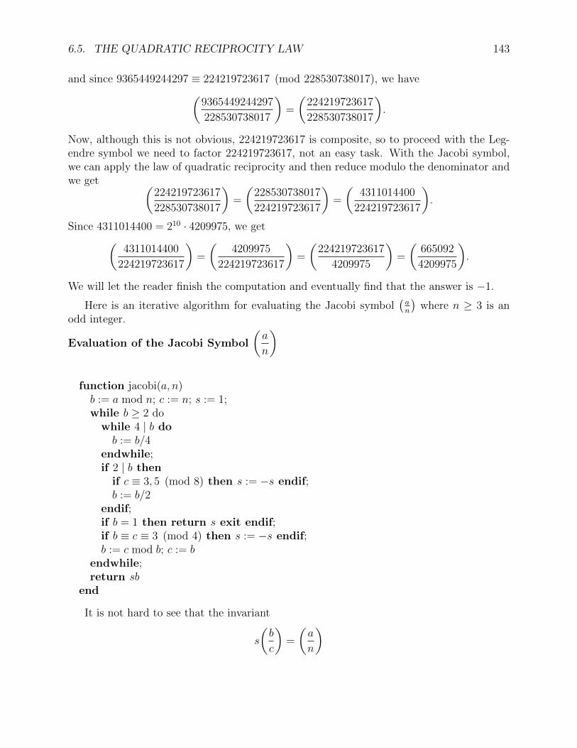
6.5. THE QUADRATIC RECIPROCITY LAW 143
and since 9365449244297 ≡ 224219723617 (mod 228530738017), we have(9365449244297
228530738017
)=
(224219723617
228530738017
).
Now, although this is not obvious, 224219723617 is composite, so to proceed with the Leg-endre symbol we need to factor 224219723617, not an easy task. With the Jacobi symbol,we can apply the law of quadratic reciprocity and then reduce modulo the denominator andwe get (
224219723617
228530738017
)=
(228530738017
224219723617
)=
(4311014400
224219723617
).
Since 4311014400 = 210 · 4209975, we get(4311014400
224219723617
)=
(4209975
224219723617
)=
(224219723617
4209975
)=
(665092
4209975
).
We will let the reader finish the computation and eventually find that the answer is −1.
Here is an iterative algorithm for evaluating the Jacobi symbol(an
)where n ≥ 3 is an
odd integer.
Evaluation of the Jacobi Symbol
(a
n
)
function jacobi(a, n)b := a mod n; c := n; s := 1;while b ≥ 2 do
while 4 | b dob := b/4
endwhile;if 2 | b then
if c ≡ 3, 5 (mod 8) then s := −s endif;b := b/2
endif;if b = 1 then return s exit endif;if b ≡ c ≡ 3 (mod 4) then s := −s endif;b := c mod b; c := b
endwhile;return sb
end
It is not hard to see that the invariant
s
(b
c
)=
(a
n
)
144 CHAPTER 6. THE SOLOVAY–STRASSEN TEST
is maintained during execution of the program. Also, if gcd(a, n) > 1, then at some pointb becomes 0, so there is no need to compute gcd(a, n). We leave it as an exercise to provethat the above program computes the Jacobi symbol
(an
); for help, consult Dietzfelbinger
[4] (Section 6.3). It is also easy to prove that the number of iterations of the main whileloop is O(log n) and that that the program runs in O((log n)2) bit operations if |a| < n (seeCrandall and Pomerance [3], Chapter 2).
It is remarkable that deciding whether a is a quadratic residue modulo p (p prime) canbe done quickly (in polynomial time in log p), basically the same complexity as computingthe gcd. However finding a square root in Z/pZ is hard (with p prime). So far, no knowndeterministic polynomial-time algorithm is known. It is known that if the ERH holds, thenthere is a quadratic nonresidue d < 2(log p)2. From this, a square root can be found inpolynomial time, if it exists.
6.6 A Randomized Algorithm to Find a Square
Root mod p
If p is an odd prime, we saw in Section 6.1 that if p is of the form p = 4k + 3, then a squareroot of a quadratic residue a is easily found: a(p+1)/4 is a square root of a mod p. We nowshow that if p = 4k+ 1 is prime, then there is a randomized algorithm to find a square rootof a quadratic residue a mod p.
First, we show that if p = 8k+ 3 or if p = 8k+ 7 is prime, then it is easy to find a squareroot of a quadratic residue a mod p. We can write p− 1 = 2(4k + 1) or p− 1 = 2(4k + 3),that is, p− 1 = 2t where t is odd. Since a is a quadratic residue mod p, by Euler’s criterion
a(p−1)/2 ≡ at ≡ 1 (mod p).
Thus at+1 ≡ a (mod p), and since t is odd, t+ 1 is even, so y = a(t+1)/2 = a(p+1)/4 mod p isa square root of a.
If p = 8k + 5 is prime, then p− 1 = 4(2k + 1), that is, p− 1 = 4t = 2st with s = 2 andt odd, and if p = 8k + 1 is prime, then p − 1 = 8k. In the second case, p − 1 = 2st withs ≥ 3 and t odd. Since a is a quadratic residue mod p, by Euler’s criterion we still havea(p−1)/2 ≡ 1 (mod p), namely
a2s−1t ≡ 1 (mod p).
We deduce that a1+2s−1t ≡ a (mod p), but since s ≥ 2, the number 1 + 2s−1t is odd, so thisdoes not help.
What we have though, is(at)2
s−1 ≡ 1 (mod p). (∗)
This implies that the order of A = at is a divisor of 2s−1, and let this order be 2h, with0 ≤ h ≤ s− 1.
6.6. A RANDOMIZED ALGORITHM TO FIND A SQUARE ROOT mod p 145
Surprisingly, having a quadratic nonresidue d mod p helps. By Euler’s criterion, since(p− 1)/2 = 2s−1t, we have
(dt)2s−1 ≡ d2
s−1t ≡ d(p−1)/2 ≡ −1 (mod p).
If we let D ≡ dt (mod p), then we see that
D2s−1 ≡ −1 (mod p),
so D has order exactly 2s, and so does D−1. This is because since D is invertible, Dk ≡ 1(mod p) iff 1 ≡ (D−1)k (mod p). Since (Z/pZ)∗ is a cyclic group, by Proposition 4.18(e),it contains a single subgroup of order 2s generated by D−1, and since A has order at most2s−1, it must belong to this subgroup, so it must be some power of D−1. Thus A ≡ (D−1)r
(mod p) for some r such that 1 ≤ r ≤ 2s.
Since the order of A is 2h we have
A2h ≡ ((D−1)r)2h ≡ (D−1)r2
h ≡ 1 (mod p),
and since D−1 has order 2s, we see that 2s divides r2h. Therefore r = r12s−h, and since
r ≤ 2s, we have 1 ≤ r1 ≤ 2h with 0 ≤ h ≤ s − 1. If r1 is even, say r1 = 2r2, thenr = r22
s−h+1, and then
A2h−1 ≡ ((D−1)r22s−h+1
)2h−1 ≡ (D−1)r22
s ≡ ((D−1)2s
)r2 ≡ 1 (mod p),
contradicting the fact that A has order 2h.
Therefore, we showed that A ≡ (D−1)r (mod p), with r = r12s−h, for some odd r1 such
that 1 ≤ r1 < 2h, and 0 ≤ h ≤ s− 1.
If h = 0, then r1 = 1 and r = 2s, in which case A ≡ (D−1)2s ≡ 1 (mod p), so equivalently
we set r = 0. Thus either r = 0, or r = r12s−h for some odd r1 with 1 ≤ r1 < 2h and
1 ≤ h ≤ s− 1. Observe that if r 6= 0 then r < 2s.
If we decompose r = r12s−h 6= 0 into a sum of powers of 2, which amounts to writing r
in binary, we obtainr = 2s−h + 2i2 + · · ·+ 2ik
for some increasing sequence s − h < i2 < · · · < ik. Since r < 2s, we have 1 ≤ k ≤ s − 1,and since h ≤ s − 1, the number r is even. We let µ = r/2, and because r < 2s, we haveµ < 2s−1.
Since A ≡ (D−1)r ≡ D−2µ (mod p), we have
AD2µ ≡ 1 (mod p), (∗∗)
that is, atD2µ ≡ 1 (mod p), and thus
at+1D2µ ≡ a (mod p).

146 CHAPTER 6. THE SOLOVAY–STRASSEN TEST
Since t is odd, t+ 1 is even, and so y = a(t+1)/2Dµ is a square root of a mod p.
Observe that (∗∗) is equivalent to
D2µ ≡ A−1 (mod p),
that is, we are trying to find a discrete logarithm for A−1 to the base D. In general, findinga discrete logarithm is very hard. Luckily, in the present case, the discrete logarithm 2µ canbe easily found. What happens is that the pieces 2ij in the binary decomposition of r = 2µcan be found using a simple test.
Let us examine the case s = 2 more closely. In this case, p − 1 = 4t with t odd, that isp = 4(2h+ 1) + 1 = 8h+ 5. By Theorem 6.13, we have(
2
p
)= −1,
that is, 2 is a quadratic nonresidue. Then with A ≡ at (mod p) and D = 2t (mod p), wehave AD2µ ≡ 1 (mod p) for some µ such that 0 ≤ µ < 2s−1 = 21 = 2. Either µ = 0 andthen a(t+1)/2 is a square root of a, or a(t+1)/22t is is a square root of a. Since p = 4t + 1,we have t = (p − 1)/4 and (t + 1)/2 = (p + 3)/8, so either a(p+3)/8 is a square root of a, ora(p+3)/82(p−1)/4 is a square root of a.
In summary, we have the following algorithm. Given an odd prime p, write p − 1 = 2stwith s ≥ 1 and t odd.
(1) If s = 1, then p ≡ 3, 7 (mod 8), and y = a(t+1)/2 = a(p+1)/4 mod p is a square root ofa mod p.
(2) If s = 2, then p ≡ 5 (mod 8), and either a(p+3)/8, or a(p+3)/82(p−1)/4, is a square root ofa mod p.
(3) If s ≥ 3, then p ≡ 1 (mod 8). Choose at random some integer d ∈ 2, . . . , p− 1 suchthat d is quadratic nonresidue mod p. We can check this by computing the Legendresymbol
(dp
)(using the fast method for computing Jacobi symbols).
Compute A ≡ at (mod p) and D ≡ dt (mod p). Search for µ such that 0 ≤ µ < 2s−1
and AD2µ ≡ 1 (mod p) as follows:
Initialize m as m := 0. For i = 1, . . . , s−1, check whether (ADm)2s−1−i ≡ −1 (mod p).
If yes, then increment m by 2i; m := m + 2i. Otherwise, increment i by 1; i :=i + 1. When i = s, stop; we found m = 2µ such that ADm ≡ 1 (mod p), andy = a(t+1)/2Dm/2 mod p is a square root of a mod p.
6.6. A RANDOMIZED ALGORITHM TO FIND A SQUARE ROOT mod p 147
The correctness of Step 3 of the algorithm can be shown as follows. If A has order 1,then r = 0 and A ≡ at ≡ 1 (mod p). For m = 0, since AD0 ≡ A ≡ 1 (mod p), the test(ADm)2
s−1−i ≡ −1 (mod p) fails for i = 1, . . . , s− 1, so the program ends with m = 0, anda(t+1)/2 is indeed a square root of a mod p.
If A has order 2h greater than 1, then 1 ≤ h ≤ s − 1, r = 2s−hr1 with r1 odd, soA = (D−1)r12
s−h, with 1 ≤ r1 < 2h. For m = 0,
(AD0)2s−1−i ≡ ((D−1)r12
s−h)2s−1−i ≡ (D−1)r12
s+s−h−i−1
(mod p).
For i = s− h, we have s+ s− h− i− 1 = s− 1, and since r1 is odd the test
(AD0)2s−1−(s−h) ≡ (D−1)r12
s−1 ≡ ((D−1)2s−1
)r1 ≡ (D−1)2s−1 ≡ −1 (mod p)
succeeds, but for 1 ≤ i ≤ s− h− 1, we have
(AD0)2s−1−i ≡ (D−1)r12
s+s−h−i−1 ≡ ((D−1)2s
)r12s−h−i−1 ≡ 1 (mod p),
so the test(AD0)2
s−1−i ≡ −1 (mod p)
fails for 1 ≤ i ≤ s − h − 1. Thus we set m = 2s−h. If r1 = 1, we are done. Otherwiser = 2s−h + r22
i2 with i2 > s− h and r2 odd. Next we look at
(AD2s−h)2s−1−i ≡ ((D−1)2
s−h+r22i2D2s−h)2s−1−i ≡ (D−1)r22
s−1+i2−i (mod p).
Since i2 > s− h, for i2 − i > 0, that is, i = s− h+ 1, . . . , i2 − 1, we have
(AD2s−h)2s−1−i ≡ (D−1)r22
s−1+i2−i ≡ 1 (mod p),
so the test fails, but for i = i2, we have
(AD2s−h)2s−1−i2 ≡ (D−1)r22
s−1 ≡ −1 (mod p),
and the test succeed, so we set m = m + 2i2 . If r2 = 1 we are done. Otherwise r =2s−h + 2i2 + r32
i3 with i3 > i2 and r3 odd. We repeat the test
(ADm)s−1−i ≡ −1 (mod p)
starting with i = i2 + 1. As in the previous case we will have
(ADm)s−1−i ≡ 1 (mod p)
for i = i2 + 1, . . . , i3 − 1, but
(ADm)s−1−i3 ≡ −1 (mod p),

148 CHAPTER 6. THE SOLOVAY–STRASSEN TEST
so we set m = m+ 2i3 . What is going on is now clear, and by an argument by induction leftto the reader, we can prove that when the algorithm stops with i = s, we have
m = r = 2s−h + 2i2 + · · ·+ 2ik .
Then a(t+1)/2Dm/2 mod p is a square root of a mod p.
It is informative to apply the above algorithm to p = 17. It is easily seen that thequadratic residues mod 17 are
1, 4, 9, 16, 8, 2, 15, 13.
Let us apply the algorithm to a = 2. We have p−1 = 16 = 24 ·1, so s = 4 and t = 1. It easyto see that 2 has order 8 = 23 mod 17, and the inverse of 2 mod 17 is 9. Let us pick d = 5,which is indeed a quadratic nonresidue mod 17. We could have picked d = 3, but d = 5 isless trivial. Since t = 1, we have
A = a1 = 2, D = d1 = 5.
It is easy to check that 5 has order 16 = 24 mod 17. The inverse of 5 modulo 17 is 7, and weare trying to find r such that 2 · 5r ≡ 1 (mod 17), which is equivalent to 2 ≡ 7r (mod 17),and to 5r ≡ 9 (mod 17). It turns out that r = 10 works. Let us see how the algorithm findsr = 10 = 21 + 23.
Recall that we are performing the test
(ADm)2s−1−i ≡ −1 (mod p),
that is(2 · 5m)2
3−i ≡ −1 (mod 17),
starting with m = 0, and from i = 1, . . . , s − 1. The index i runs from i = 1 to i = 3, andso 3− i runs from 2 to 0.
For m = 0 and i = 1, that is 3− i = 2, the algorithm finds that 222 ≡ 16 ≡ −1 (mod 17).Thus we set m = 21 = 2, and we test whether (2 · 52)2
3−i ≡ −1 (mod 17) for i = 2, 3. Wefind that (2 · 52)2 ≡ 1 (mod 17) for i = 2 and that (2 · 52)1 ≡ −1 (mod 17) for i = 3, so weset m = m+ 23 = 2 + 23 = 10.
The algorithm found m = 10, so y = 2 · 55 (mod 17) is a square root of 2 mod 17. Wecan check that 2 · 55 ≡ 11 (mod 17), and 112 ≡ 2 (mod 17), so 11 is a square root of 2mod 17.
As an exercise, the reader should check that with d = 3, again the order of 3 is 16 = 24, theinverse of 3 mod 17 is 6, and 2 ≡ 62 (mod 17). In this case m = r = 2. Since 222 ≡ 24 ≡ −1(mod 17) for i = 1, we get m = 21 = 2. Since 2 · 32 ≡ 18 ≡ 1 (mod 17), the algorithmterminates with m = 2, and we find 2 · 3 = 6 as square root of 2 mod 17.

6.6. A RANDOMIZED ALGORITHM TO FIND A SQUARE ROOT mod p 149
Here is another example from Koblitz [10] (Chapter II, Section 2). Let p = 401 anda = 186. By computing the Legendre symbol
(186401
), we find that a is a quadratic residue
mod 401. We also find that 3 is a quadratic nonresidue mod 401 by computing the Legendresymbol
(3
401
). We have p− 1 = 401− 1 = 400 = 24 × 25, so s = 4 and t = 25. We find that
A ≡ 18625 ≡ 98 (mod 401), D ≡ 325 ≡ 268 (mod 401).
We have s− 1− i = 3− i and we are testing whether
(98 · 268m)23−i ≡ −1 (mod 401),
starting from m = 0, with i = 1, 2, 3.
For i = 1, we have 3− i = 2, and we check that
984 ≡ −1 (mod 401),
so we set m = 21 = 2. Next i = 2, so 3− i = 1, and we compute
(98× 2682)2 ≡ (982 mod 401)× (2684 mod 401) ≡ 381× 20 ≡ 1 (mod 401),
so we increment i to i = 3, and we compute
(98× 2682)1 ≡ 98× (2682 mod 401) ≡ 98× 45 ≡ −1 (mod 401),
so m = m+ 23 = 2 + 8 = 10. The algorithm stops with m = 10.
We check that 26810 ≡ 356 (mod 401), and that 356 is the inverse of 98 mod 401, soindeed
98× 26810 ≡ 1 (mod 401).
The square root a(t+1)/2Dm/2 mod p is equal to
18623 × 2685 mod 401 = (18623 mod 401)× (2685 mod 401) = 103× 147 mod 401 = 304.
We easily confirm that y = 304 is a square root of 186 mod 401.
According to Crandall and Pomerance [3] (Chapter 2, Algorithm 2.3.8), the above algo-rithm was originally invented by Tonelli in 1891, based on ideas of Gauss. They also giveanother randomized algorithm using arithmetic in the finite field Fp2 due to Cipolla (1907).
If n is composite, there is no known fast method for computing square roots. In fact, itcan be shown that doing so is essentially equivalent to factoring n in the following sense: ifthere is a polynomial time, possibly randomized, algorithm to compute square roots moduloany n, then there is a randomized polynomial time algorithm for factoring n. This is Theorem14.21 in Motwani and Raghavan [15].
150 CHAPTER 6. THE SOLOVAY–STRASSEN TEST
6.7 Proof of the Quadratic Reciprocity Law
At least 150 proofs of the quadratic reciprocity law have been published. Gauss himself gaveseven different proofs. We follow a short proof using “Gauss sums” due to Jean-Pierre Serre[20]. This proof is not entirely elementary because it uses the fact that if p and q are distinctodd primes, then there is a field extension Ω of Fp = Z/pZ in which there is an element oforder q (a primitive qth root of unity). Any algebraic closure of Fp will do. Since pq−1 ≡ 1(mod q) (by Fermat’s little theorem), q divides pq−1 − 1, so the finite field Fpq−1 also workssince its multiplicative group is cyclic of order pq−1 − 1.
Theorem 6.14. (Quadratic reciprocity law for primes (Gauss)) For any two distinct oddprimes p, q, we have (
p
q
)= (−1)
p−12
q−12
(q
p
).
Proof. Let Ω be any field extension of Fp = Z/pZ in which there is a primitive qth root ofunity, for example Ω = Fpq−1 . If w ∈ Ω is a primitive qth root of unity, define the Gauss sumy by
y =∑a∈Fq
(a
q
)wa,
with(0q
)= 0. Then, we have two steps.
Step 1. We prove that
y2 = (−1)(q−1)/2q.
Step 2. We prove that
yp−1 =
(p
q
).
If we assume that Step 1 and Step 2 have been established, by Step 1, y is a square root of(−1)(q−1)/2q, and by a Proposition 6.4(1)(
(−1)(q−1)/2q
p
)= yp−1,
so by Step 2 ((−1)(q−1)/2q
p
)=
(p
q
).
On the other hand, by Proposition 6.5 and Proposition 6.6, we have(p
q
)=
((−1)(q−1)/2q
p
)=
((−1)(q−1)/2
p
)(q
p
)= (−1)(p−1)(q−1)/4
(q
p
),
which proves the desired formula.

6.7. PROOF OF THE QUADRATIC RECIPROCITY LAW 151
Proof of Step 1. We have
y2 =
(∑a∈Fq
(a
q
)wa)(∑
b∈Fq
(b
q
)wb)
=∑a,b∈Fq
(ab
q
)wa+b =
∑c∈Fq
wc(∑a∈Fq
(a(c− a)
q
)),
by making the change of variable c = a+ b. Now, if a 6= 0, we have a(c−a) = −a2(1− ca−1),and since
(aq
)= ±1 since a ∈ Fq, we have
(aq
)2= 1, so(
a(c− a)
q
)=
(−a2(1− ca−1)
q
)=
(a
q
)2(−1
q
)(1− ca−1
q
)= (−1)(q−1)/2
(1− ca−1
q
),
and thus,
(−1)(q−1)/2y2 =∑c∈Fq
Scwc,
with
Sc =∑a∈F∗q
(1− ca−1
q
).
If c = 0, then
S0 =∑a∈F∗q
(1
q
)= q − 1.
Otherwise, d = 1− ca−1 runs over Fq − 1, and we have
Sc =∑a∈F∗q
(1− ca−1
q
)=∑d∈Fq
(d
q
)−(
1
q
)=∑d∈F∗q
(d
q
)−(
1
q
)= −
(1
q
)= −1,
since in F∗q there are as many squares as nonsquares (see Proposition 6.1). As a consequence.∑c∈Fq
Scwc = S0 +
∑c∈F∗q
Scwc = q − 1−
∑c∈F∗q
wc = q,
since∑
c∈F∗qwc = −1 (because w is a primitive qth root of unity, so wq = 1,
0 = wq − 1 = (w − 1)(wq−1 + · · ·+ w + 1),
which implies wq−1 + · · · + w + 1 = 0, and thus,∑
c∈F∗qwc = wq−1 + · · · + w = −1), which
proves Step 1.
Proof of Step 2. Since Ω is a field of characteristic p, we have
(x1 + x2)p = xp1 + xp2.
152 CHAPTER 6. THE SOLOVAY–STRASSEN TEST
Then if m ≥ 3 we have
(x1 + · · ·+ xm)p = (x1 + · · ·+ xm−1)p + xpm,
and by induction(x1 + · · ·+ xm)p = xp1 + · · ·+ xpm,
for all x1, . . . , xm ∈ Ω. Consequently, since p is odd(aq
)p=(aq
), we get
yp =∑a∈Fq
(a
q
)pwap =
∑a∈Fq
(a
q
)wap,
and by making the change of variable b = ap, we get
yp =∑b∈Fq
(bp−1
q
)wb =
∑b∈Fq
(p
q
)2(bp−1
q
)wb =
∑b∈Fq
(bp
q
)wb =
(p
q
)∑b∈Fq
(b
q
)wb =
(p
q
)y.
Therefore, yp−1 =
(p
q
), as claimed.
The proof of the quadratic reciprocity law for the Jacobi symbol is now easy to obtain.For the reader’s convenience, we repeat the statement of the theorem.
Theorem 6.15. (Quadratic reciprocity law for the Jacobi symbol) If m and n are any oddintegers m,n ≥ 3 such that gcd(m,n) = 1, then(
m
n
)= (−1)
m−12
n−12
(n
m
).
Equivalently, (m
n
)=
(n
m
)if m ≡ 1 mod 4 or n ≡ 1 mod 4
−(n
m
)if m ≡ 3 mod 4 and n ≡ 3 mod 4.
Proof. Write the prime factorizations of m and n as m = p1 · · · ps and n = q1 · · · qt, wherethe pi and qj are primes. Then, we have(
m
n
)(n
m
)=
s∏i=1
t∏j=1
(piqj
)(qjpi
)= (−1)r,
for some integer r. Applying the quadratic reciprocity law for primes to each factor, we findthat
r =s∑i=1
t∑j=1
(pi − 1)
2
(qj − 1)
2=
s∑i=1
pi − 1
2
t∑j=1
qj − 1
2.

6.7. PROOF OF THE QUADRATIC RECIPROCITY LAW 153
During the proof of part (7) of Proposition 6.9, we showed that
s∑i=1
pi − 1
2≡ m− 1
2(mod 2)
t∑j=1
qj − 1
2≡ n− 1
2(mod 2).
Therefore,
r ≡ (m− 1)
2
(n− 1)
2(mod 2),
which proves our formula.
Another way of proving the law of quadratic reciprocity (for primes) is to use Gauss sets.Given any odd prime p, any subset S of F∗p = 1, 2, . . . , p− 1 such that S ∩ (−S) = ∅ and
F∗p = S ∪ −S
is called a Gauss set . Observe that since |S| = | − S|, the fact that F∗p is the disjoint unionof S and −S implies that |S| = (p− 1)/2. In particular,
S =
1, 2, . . . ,
p− 1
2
is a Gauss set. Then, for any s ∈ S and any a ∈ F∗p, we can write
as = es(a)sa,
for some sa ∈ S and with es(a) = ±1. (Of course, as is multiplication in Fp, so as ≡ es(a)sa(mod p).)
Lemma 6.16. (Gauss’s lemma) For any odd prime p and any a ∈ F∗p, we have(a
p
)=∏s∈S
es(a).
Proof. First, observe that if s 6= s′, then sa 6= s′a, because if sa = s′a, since as = es(a)sa,as′ = es′(a)s′a = es′(a)sa, and es(a), es′(a) ∈ −1, 1, we would have as = as′, thus s = ±s′,contradicting the fact that S and −S disjoint. Therefore, the map s 7→ sa is a bijection ofS. If we multiply the equations
as = es(a)sa
for all s ∈ S, we get
a(p−1)/2∏s∈S
s =
(∏s∈S
es(a)
)∏s∈S
sa =
(∏s∈S
es(a)
)∏s∈S
s,

154 CHAPTER 6. THE SOLOVAY–STRASSEN TEST
which implies that
a(p−1)/2 =∏s∈S
es(a).
However, we know that (a
p
)= a(p−1)/2,
which proves the lemma.
As an application of Lemma 6.16, the reader should reprove that(2
p
)= (−1)(p−1)/2,
by setting a = 2 and using the set S from above. It turns out that(2
p
)= (−1)n(p),
where n(p) is the number of integers s such that
p− 1
4< s ≤ p− 1
2.
We can use the Gauss set
S =
1, 2, . . . ,
p− 1
2
and Lemma 6.16 to compute the Legendre symbol
(pq
). Given any a ∈ 1, . . . , p−1, consider
the residues mod p of the multiples of a,a, 2a, . . . ,
p− 1
2a
,
say r1, . . . , r(p−1)/2.
If rs ∈ S, then as = sa ≡ rs (mod p) so es(a) = +1, and if rs /∈ S, then p− rs ∈ S, andas = sa ≡ rs ≡ −(p− rs) (mod p), we have es(a) = −1. It follows that
∏s∈S ea(s) = (−1)µ,
where µ is the number of residues rs not in S.
Therefore, we proved that (a
p
)= (−1)µ,
where µ is the number of residues rs mod p of the multiples of a,a, 2a, . . . ,
p− 1
2a
,
6.8. EISENSTEIN’S PROOF OF THE QUADRATIC RECIPROCITY LAW 155
such that rs is not in S. This is how Lemma 6.16 is stated in Apostol [1] (Chapter 9, Theorem9.6) and Niven, Zuckerman, and Montgomery [16] (Section 3.1, Theorem 3.2).
There is a formula that gives the parity of m in terms of a and p; see Apostol [1] (Chapter9, Theorem 9.7) and Niven, Zuckerman, and Montgomery [16] (Section 3.1, Theorem 3.3).Using Lemma 6.16 and this formula, a short proof of the law of quadratic reciprocity can beobtained; see Apostol [1] (Chapter 9, Theorem 9.8), and Niven, Zuckerman, and Montgomery[16] (Section 3.2, Theorem 3.4). This is essentially Gauss’ third proof; see Dirichlet–Dedekind[12] (Chapter 3, Sections 42 and 43). In some sense, this proof is more elementary than theone we gave. Generalizations of the law of quadratic reciprocity are discussed in Ireland andRosen [9]. The historical notes found at the end of every chapter of Ireland and Rosen [9]are also very informative.
6.8 Eisenstein’s Proof of the Quadratic
Reciprocity Law
Another strikingly short proof due to Eisenstein (1845) using a trigonometric identity isgiven in Serre [20] (Chapter 1, Appendix). This proof is just too beautiful to be left aside,so here is Serre’s proof of the quadratic reciprocity law after Eisenstein (1845).
Eisenstein’s proof. The idea is to use Gauss’s lemma, which says that(a
p
)=∏s∈S
es(a),
where ea(s) = ±1 is defined so that as = es(a)sa, with s and sa in the Gauss set
S =
1, 2, . . . ,
p− 1
2
.
The key ingredient (stroke of genius) of the proof is that if as = es(a)sa, then
sin
(2π
pas
)= es(a) sin
(2π
psa
). (∗sin)
We simply used the fact that the sine function has the property that sin(−x) = − sinx. But(∗sin) yields
ea(a) =sin(
2πasp
)sin(
2πsap
) ,so we obtain (
a
p
)=∏s∈S
es(a) =∏s∈S
sin(
2πasp
)sin(
2πsap
) =∏s∈S
sin(
2πasp
)sin(
2πsp
) ,
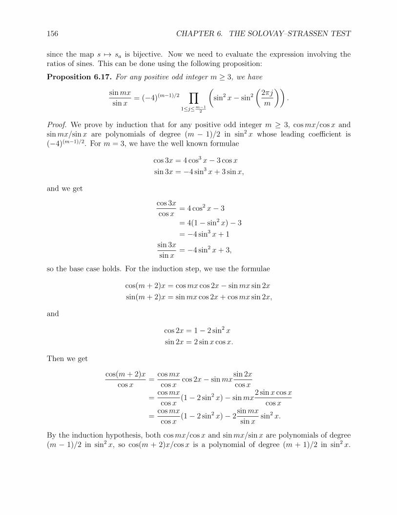
156 CHAPTER 6. THE SOLOVAY–STRASSEN TEST
since the map s 7→ sa is bijective. Now we need to evaluate the expression involving theratios of sines. This can be done using the following proposition:
Proposition 6.17. For any positive odd integer m ≥ 3, we have
sinmx
sinx= (−4)(m−1)/2
∏1≤j≤m−1
2
(sin2 x− sin2
(2πj
m
)).
Proof. We prove by induction that for any positive odd integer m ≥ 3, cosmx/cosx andsinmx/sinx are polynomials of degree (m − 1)/2 in sin2 x whose leading coefficient is(−4)(m−1)/2. For m = 3, we have the well known formulae
cos 3x = 4 cos3 x− 3 cosx
sin 3x = −4 sin3 x+ 3 sinx,
and we get
cos 3x
cosx= 4 cos2 x− 3
= 4(1− sin2 x)− 3
= −4 sin3 x+ 1
sin 3x
sinx= −4 sin2 x+ 3,
so the base case holds. For the induction step, we use the formulae
cos(m+ 2)x = cosmx cos 2x− sinmx sin 2x
sin(m+ 2)x = sinmx cos 2x+ cosmx sin 2x,
and
cos 2x = 1− 2 sin2 x
sin 2x = 2 sin x cosx.
Then we get
cos(m+ 2)x
cosx=
cosmx
cosxcos 2x− sinmx
sin 2x
cosx
=cosmx
cosx(1− 2 sin2 x)− sinmx
2 sinx cosx
cosx
=cosmx
cosx(1− 2 sin2 x)− 2
sinmx
sinxsin2 x.
By the induction hypothesis, both cosmx/cosx and sinmx/sinx are polynomials of degree(m − 1)/2 in sin2 x, so cos(m + 2)x/cosx is a polynomial of degree (m + 1)/2 in sin2 x.

6.8. EISENSTEIN’S PROOF OF THE QUADRATIC RECIPROCITY LAW 157
The leading terms of the polynomials in sin2 x for cosmx/cosx and sinmx/sinx are both(−4)(m−1)/2, so the leading term of cos(m+ 2)x/cosx in sin2 x is
−2(−4)(m−1)/2 − 2(−4)(m−1)/2 = (−4)(m+1)/2,
establishing the induction step. We also get
sin(m+ 2)x
sinx=
sinmx
sinxcos 2x+ cosmx
sin 2x
sinx
=sinmx
sinx(1− 2 sin2 x) + cosmx
2 sinx cosx
sinx
=sinmx
sinx(1− 2 sin2 x) + 2
cosmx
cosxcos2 x
=sinmx
sinx(1− 2 sin2 x) + 2
cosmx
cosx(1− sin2 x).
By the induction hypothesis, both cosmx/cosx and sinmx/sinx are polynomials of degree(m − 1)/2 in sin2 x, so sin(m + 2)x/sinx is a polynomial of degree (m + 1)/2 in sin2 x.The leading terms of the polynomials in sin2 x for cosmx/cosx and sinmx/sinx are both(−4)(m−1)/2, so the leading term of sin(m+ 2)x/sinx in sin2 x is
−2(−4)(m−1)/2 − 2(−4)(m−1)/2 = (−4)(m+1)/2,
establishing the induction step.
Finally, observe that sinmx/sinx vanishes for x = 2πj/m with j = 1, . . . , (m− 1)/2, sothe polynomial in sin2 x expressing sinmx/sinx vanishes for sin2 x = sin2
(2πjm
), and since
this polynomial has degree (m− 1)/2, it is the product of the factors
sin2 x− sin2
(2πj
m
),
up to its leading coefficient. But we just showed that this leading coefficient is (−4)(m−1)/2,which proves our formula.
Let T be the set
T =
1, 2, . . . ,
a− 1
2
.
Using Proposition 6.17 with m = a and x = (2πs)/p, we obtain(a
p
)=∏s∈S
es(a) =∏s∈S
(−4)(a−1)/2∏t∈T
(sin2
(2πs
p
)− sin2
(2πt
a
))= (−4)(a−1)(p−1)/4
∏s∈S
∏t∈T
(sin2
(2πs
p
)− sin2
(2πt
a
)),

158 CHAPTER 6. THE SOLOVAY–STRASSEN TEST
since S has (p− 1)/2 elements. Thus we have(a
p
)= (−4)(a−1)(p−1)/4
∏s∈S
∏t∈T
(sin2
(2πs
p
)− sin2
(2πt
a
)). (∗1)
Exchanging the roles of a and p, we obtain(p
a
)= (−4)(a−1)(p−1)/4
∏s∈S
∏t∈T
(sin2
(2πt
a
)− sin2
(2πs
p
)). (∗2)
Comparing (∗1) and (∗2), we see that the factors are identical except for their sign. Sincethere are (a− 1)(p− 1)/4 factors, we deduce that(
p
a
)= (−1)(a−1)(p−1)/4
(p
a
),
which is indeed the law of quadratic reciprocity.
6.9 Strong Pseudoprimes are Euler Pseudoprimes
We conclude this chapter by showing that every strong pseudoprime base a is also an Eulerpseudoprime base a. This is another indication that the Miller–Rabin test is somewhatbetter than the Solovay–Strassen test (recall that the proportion of MR-liars is at most 1/4,whereas the proportion of E-liars is at most 1/2). We follow Koblitz’s proof [10] (ChapterV).
We begin with an easy result, but first, observe that if a is an E-liar, then(a
n
)a(n−1)/2 ≡ 1 (mod n),
which implies that gcd(a, n) = 1, and since(an
)∈ −1, 1, the above condition is equivalent
to (a
n
)≡ a(n−1)/2 (mod n).
Proposition 6.18. If n is any composite of the form n = 4k + 3, then n is a strongpseudoprime base a iff n is an Euler pseudoprime base a.
Proof. Since n = 4k + 3, we have n − 1 = 2(2k + 1), so n − 1 = 2st with s = 1 andt = (n− 1)/2. Thus, n is a strong pseudoprime base a iff a(n−1)/2 ≡ ±1 (mod n). If n is anEuler pseudoprime, then the above congruence holds, by definition.
Conversely, assume that a(n−1)/2 ≡ ±1 (mod n). Then, since (n− 3)/4 = k is an integer,we have(
a
n
)=
(a(n−3)/4
n
)2(a
n
)=
(a(n−3)/2
n
)(a
n
)=
(a(n−3)/2 · a
n
)=
(a(n−1)/2
n
),
6.9. STRONG PSEUDOPRIMES ARE EULER PSEUDOPRIMES 159
and because (n− 1)/2 = 2k + 1, we have(−1
n
)= −1,
which implies that (a
n
)≡ a(n−1)/2 (mod n),
as desired.
The case were n = 4k + 1 is more involved.
Theorem 6.19. If n is a strong pseudoprime base a, then n is an Euler pseudoprime basea.
Proof. Write n − 1 = 2st with t odd and assume that a in an MR-liar for n, which meansthat either
(a) at ≡ 1 (mod n), or
(b) a2it ≡ n− 1 (mod n), for some i with 0 ≤ i ≤ s− 1.
We consider several cases.
Case 1. Assume that at ≡ 1 (mod n). In this case, since (n− 1)/2 = 2s−1t, we have
a(n−1)/2 ≡ 1 (mod n).
We also have
1 =
(1
n
)=
(at
n
)=
(a
n
)t,
and since t is odd me must have
(a
n
)= 1, so
(a
n
)≡ a(n−1)/2 (mod n).
Case 2. Assume that (b) holds for i = s − 1; that is, a(n−1)/2 ≡ −1 (mod n). We mustshow that
(an
)= −1.
Let p be any prime divisor of n and write p−1 = 2s′t′, with t′ odd. We make the following
claim:
Claim. We have s′ ≥ s and (a
p
)=
−1 if s′ = s
1 if s′ > s.
160 CHAPTER 6. THE SOLOVAY–STRASSEN TEST
Proof of the claim. From
a(n−1)/2 = a2s−1t ≡ −1 (mod n),
raising both sides to the power t′ we we obtain(a2
s−1t
)t′≡(a2
s−1t′)t≡ −1 (mod n),
and since p divides n, we also have(a2
s−1t′)t≡ −1 (mod p).
If we had s′ < s, then we would not have
ap−1 ≡ a2s′ t′ ≡ 1 (mod p),
contradicting Fermat’s little theorem. Thus, s′ ≥ s. If s′ = s, then(a2
s−1t′)t≡ −1 (mod p),
and since t is odd this implies that(a
p
)≡(a
p
)t≡ (a(p−1)/2)t ≡
(a2
s′−1t′)t≡ −1 (mod p).
On the other hand, if s′ > s, then the congruence(a2
s−1t′)t≡ −1 (mod p)
raised to the power 2s′−s implies that
(a2
s′−1t′)t≡(a(p−1)/2
)t ≡ 1 (mod p), and since t is
odd,(ap
)t=(ap
)= 1.
Write n as a product of primes (not necessarily distinct), n = p1p2 · · · pm, and let k bethe number of primes p such that s′ = s when we write p − 1 = 2s
′t′ with t′ odd, counting
such a prime with its multiplicity. By the claim, s′ ≥ s and(a
n
)=
m∏i=1
(a
pi
)= (−1)k.
On the other hand, working modulo 2s+1, we see that p ≡ 1 (mod 2s+1) unless p is one of thek primes for which s′ = s, in which case p ≡ 1 + 2s (mod 2s+1). Since n = 1 + 2st ≡ 1 + 2s
(mod 2s+1), we have
1 + 2s ≡ p1 · · · pm ≡ (1 + 2s)k ≡ 1 + k2s (mod 2s+1),
6.9. STRONG PSEUDOPRIMES ARE EULER PSEUDOPRIMES 161
using the binomial formula in the last step. The congruence
2s ≡ k2s (mod 2s+1)
implies that k is odd, hence (a
n
)= (−1)k = −1,
as was to be proved.
Case 3. Assume that (b) holds for i < s − 1; that is, a2it ≡ −1 (mod n). Raising this
congruence to the power 2s−1−i, we get a(n−1)/2 ≡ 1 (mod n), so we have to prove that(an
)= 1. As in Case 2, write p− 1 = ss
′t′ with t′ odd for every prime factor p of n.
Claim. We have s′ ≥ i+ 1 and(a
p
)=
−1 if s′ = i+ 1
1 if s′ > i+ 1.
The proof of the above claim is identical to the proof of the claim in Case (2). Similarlyto Case (2), let k be the number of primes (not necessarily distinct) such that s′ = i+ 1. Asin Case (2), we have (
a
n
)= (−1)k.
On the other hand, since i < s− 1, we have n = 1 + 2st ≡ 1 (mod 2i+2), and also
n ≡ p1 · · · pm ≡ (1 + 2i+1)k ≡ 1 + k2i+1 (mod 2i+2),
which implies2st ≡ k2i+1 (mod 2i+2).
Since i+ 2 ≤ s, the number k must be even, and(a
n
)= (−1)k = 1,
as desired.
There are examples of composite numbers n such that n is an Euler pseudoprime basea but n is not a strong pseudoprime base a. This behavior is observed for numbers of theform (6m+ 1)(12m+ 1)(18m+ 1), where each factor is prime and m is odd; see Exercise 17in Section 1 of Chapter V of Koblitz [10].
Acknowlegments: I wish to thank Dan Guralnik for inspiring me to write up the reviewsections on groups. I learned about Theorem 4.22 from his wonderful’s lectures in ESE 680-001. Not too surprisingly, I found that this theorem is used by J.P. Serre in his outstandingLectures in Arithmetic [20]. I also thank Peter Freyd, Ron Donagi and Steve Shatz. Petermade a number of suggestions/corrections. In particular, he brought to my attention thefacts about square roots of unity stated as Proposition 5.1 and Theorem 5.2. Ron and Stevepointed out that Theorem 4.44 implies that there are four square roots of unity when n = 2m
with m ≥ 3.

162 CHAPTER 6. THE SOLOVAY–STRASSEN TEST
Bibliography
[1] Tom M. Apostol. Introduction to Analytic Number Theory. Undergraduate Texts inMathematics. Springer, first edition, 1976.
[2] Nicolas Bourbaki. Algebre, Chapitres 4-7. Elements de Mathematiques. Masson, 1981.
[3] Richard Crandall and Carl Pomerance. Prime Numbers. A Computational Perspective.Springer, second edition, 2005.
[4] Martin Dietzfelbinger. Primality Testing in Polynomial Time. From Randomized Algo-rithms to “Primes is in P”. LNCS 3000. Springer, first edition, 2004.
[5] Harold M. Edwards. Riemann’s Zeta Function. Dover, first edition, 2001.
[6] Jean H. Gallier. Discrete Mathematics. Universitext. Springer Verlag, first edition, 2011.
[7] Carl Friedrich Gauss. Recherches Arithmetiques. Edition Jacques Gabay, first edition,1807. French Translation of the Disquisitiones Arithmeticae.
[8] Jeffrey H. Hoffstein, Jill Pipher, and Joseph H. Silverman. An Introduction to Math-ematical Cryptography. Undergraduate Texts in Mathematics. Springer, first edition,2008.
[9] Kenneth Ireland and Michael Rosen. A Classical Introduction to Modern Number The-ory. GTM No. 84. Springer Verlag, second edition, 1998.
[10] Neal Koblitz. A Course in Number Theory and Cryptography. GTM No. 114. SpringerVerlag, second edition, 1994.
[11] Serge Lang. Algebra. Addison Wesley, third edition, 1993.
[12] Peter Gustav Lejeune-Dirichlet. Lectures on Number Theory, volume 16 of History ofMathematics. AMS, first edition, 1999. Translation by John Stillwell of Vorlesungenuber Zahlentheorie with supplements by Richard Dedekind, 1863.
[13] L. Lovasz, J. Pelikan, and K. Vesztergombi. Discrete Mathematics. Elementary andBeyond. Undergraduate Texts in Mathematics. Springer, first edition, 2003.
163
164 BIBLIOGRAPHY
[14] Alfred J. Menezes, Paul C. van Oorschot, and Scott A. Vanstone. Handbook of AppliedCryptography. CRC Press, fifth edition, 2001.
[15] Rajeev Motwani and Prabhakar Raghavan. Randomized Algorihms. Cambridge Univer-sity Press, first edition, 1995.
[16] Ivan Niven, Herbert S. Zuckerman, and Hugh L. Montgomery. An Introduction to theTheory of Numbers. Wiley, fifth edition, 1991.
[17] Vaughan R. Pratt. Every prime has a succinct certificate. SIAM Journal on Computing,4(3):214–220, 1975.
[18] Paulo Ribenboim. The Little Book of Bigger Primes. Springer-Verlag, second edition,2004.
[19] R.L. Rivest, A. Shamir, and L. Adleman. A method for obtaining digital signatures andpublic-key cryptosystems. Communications of the ACM, 21(2):120–126, 1978.
[20] Jean-Pierre Serre. A Course in Arithmetic. Graduate Text in Mathematics, No. 7.Springer, first edition, 1973.
[21] Victor Shoup. A Computational Introduction to Number Theory and Algebra. CambridgeUniversity Press, second edition, 2009.
[22] Joseph H. Silverman. A Friendly Introduction to Number Theory. Prentice Hall, thirdedition, 2006.