1

Notes on “Rate-Distortion Methods for Image and Video Compression,”

A. Ortega and K. RamchandranIEEE Signal Processing Magazine

Nov. 1998 pp. 23 – 50

EE523Prof. Fowler

2

I. From Shannon Theory to MPEG Coding

3

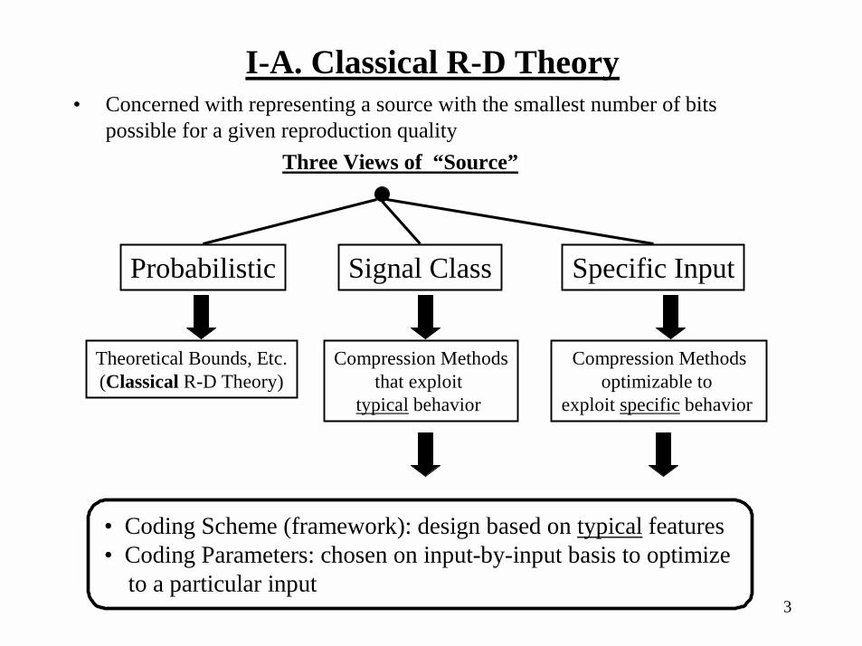
I-A. Classical R-D Theory• Concerned with representing a source with the smallest number of bits

possible for a given reproduction qualityThree Views of “Source”

Probabilistic Signal Class Specific Input

Theoretical Bounds, Etc.(Classical R-D Theory)

Compression Methodsthat exploit

typical behavior

Compression Methodsoptimizable to

exploit specific behavior

• Coding Scheme (framework): design based on typical features• Coding Parameters: chosen on input-by-input basis to optimize

to a particular input

4

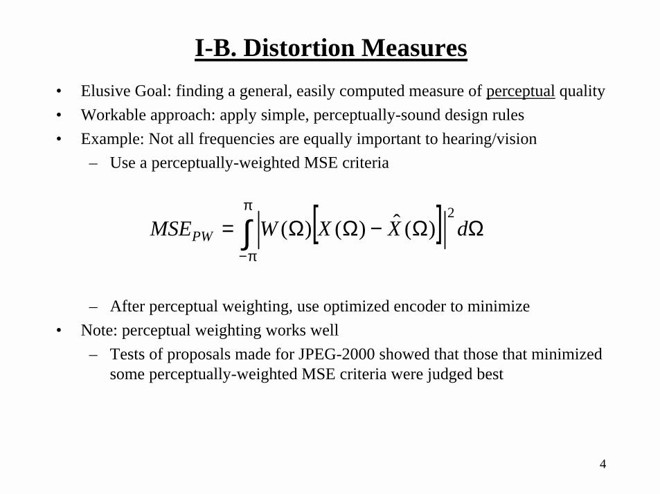
I-B. Distortion Measures• Elusive Goal: finding a general, easily computed measure of perceptual quality• Workable approach: apply simple, perceptually-sound design rules• Example: Not all frequencies are equally important to hearing/vision

– Use a perceptually-weighted MSE criteria

– After perceptual weighting, use optimized encoder to minimize• Note: perceptual weighting works well

– Tests of proposals made for JPEG-2000 showed that those that minimized some perceptually-weighted MSE criteria were judged best

[ ]∫π

π−

ΩΩ−ΩΩ= dXXWMSEPW2

)(ˆ)()(

5

I-C. Optimality & R-D Bounds• Classical: Given a statistical model, find the lower bound on R-D

– Limited to:• Simple Statistical Models• Asymptotic Results (large block or high rate)

• Practice: Optimizing performance consists of:1. Given a particular type of data, what is the appropriate model for that

type of data (probabilistic or otherwise)?2. Given the chosen model (in #1), and any applicable bounds, how close

can a practical algorithm get to the bound?

Both steps are equally important

6

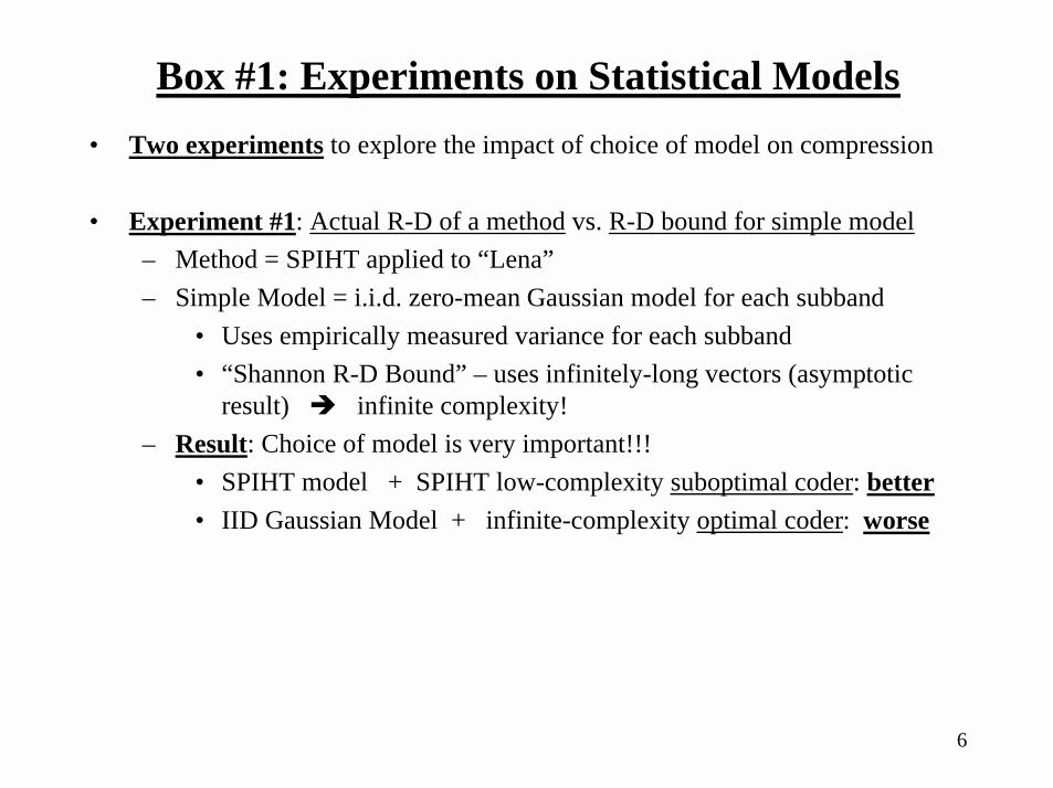
Box #1: Experiments on Statistical Models• Two experiments to explore the impact of choice of model on compression

• Experiment #1: Actual R-D of a method vs. R-D bound for simple model– Method = SPIHT applied to “Lena”– Simple Model = i.i.d. zero-mean Gaussian model for each subband

• Uses empirically measured variance for each subband• “Shannon R-D Bound” – uses infinitely-long vectors (asymptotic

result) ! infinite complexity!– Result: Choice of model is very important!!!

• SPIHT model + SPIHT low-complexity suboptimal coder: better• IID Gaussian Model + infinite-complexity optimal coder: worse

7

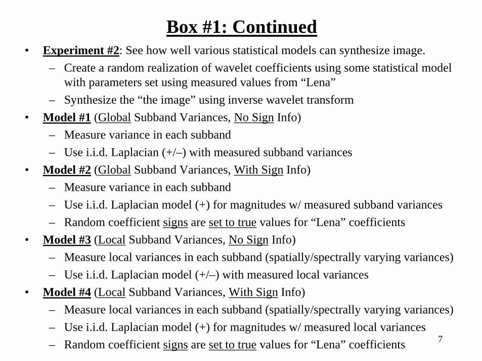
Box #1: Continued• Experiment #2: See how well various statistical models can synthesize image.

– Create a random realization of wavelet coefficients using some statistical model with parameters set using measured values from “Lena”

– Synthesize the “the image” using inverse wavelet transform• Model #1 (Global Subband Variances, No Sign Info)

– Measure variance in each subband– Use i.i.d. Laplacian (+/–) with measured subband variances

• Model #2 (Global Subband Variances, With Sign Info)– Measure variance in each subband– Use i.i.d. Laplacian model (+) for magnitudes w/ measured subband variances– Random coefficient signs are set to true values for “Lena” coefficients

• Model #3 (Local Subband Variances, No Sign Info)– Measure local variances in each subband (spatially/spectrally varying variances)– Use i.i.d. Laplacian model (+/–) with measured local variances

• Model #4 (Local Subband Variances, With Sign Info)– Measure local variances in each subband (spatially/spectrally varying variances)– Use i.i.d. Laplacian model (+) for magnitudes w/ measured local variances– Random coefficient signs are set to true values for “Lena” coefficients

8

II. Operational R-D in Practical Coder Design

9

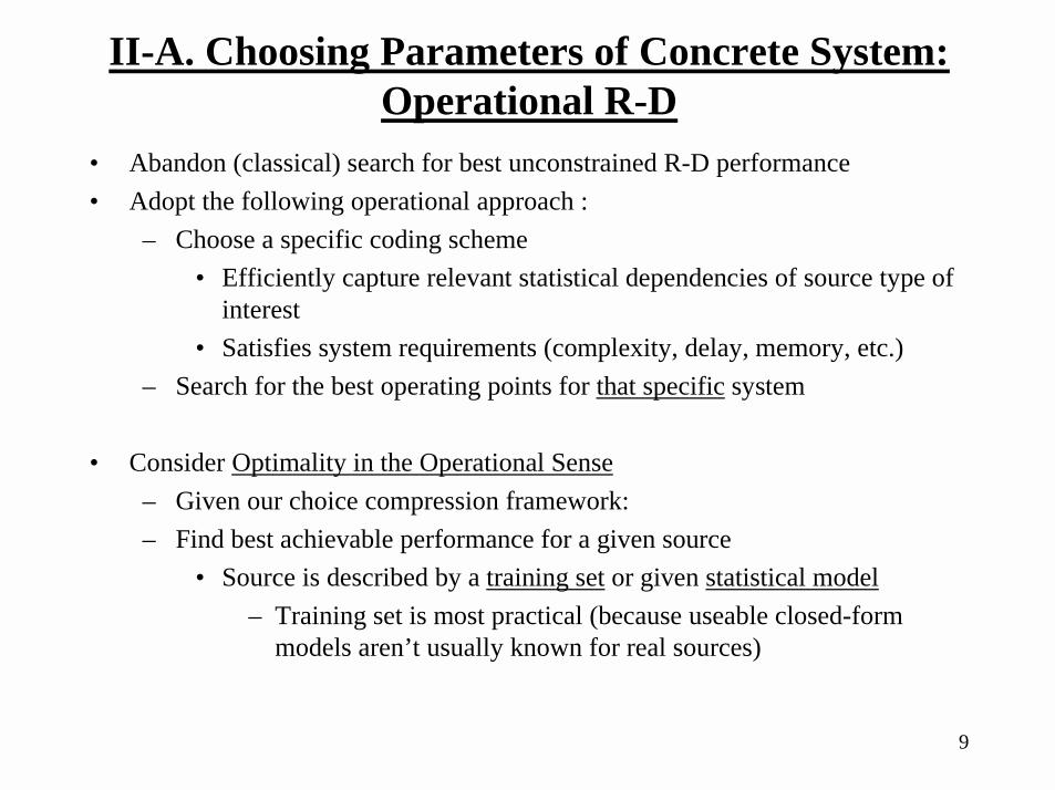
II-A. Choosing Parameters of Concrete System:Operational R-D

• Abandon (classical) search for best unconstrained R-D performance• Adopt the following operational approach :

– Choose a specific coding scheme• Efficiently capture relevant statistical dependencies of source type of

interest• Satisfies system requirements (complexity, delay, memory, etc.)

– Search for the best operating points for that specific system

• Consider Optimality in the Operational Sense– Given our choice compression framework:– Find best achievable performance for a given source

• Source is described by a training set or given statistical model– Training set is most practical (because useable closed-form

models aren’t usually known for real sources)

10

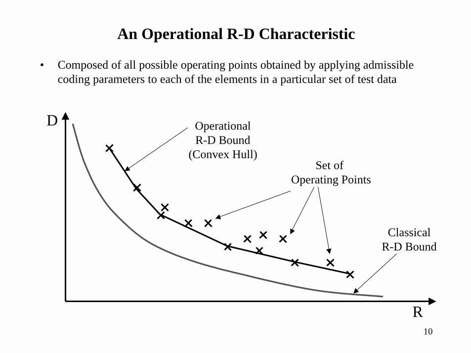
An Operational R-D Characteristic

• Composed of all possible operating points obtained by applying admissible coding parameters to each of the elements in a particular set of test data

ClassicalR-D Bound

Set of Operating Points

OperationalR-D Bound

(Convex Hull)

R

D

11

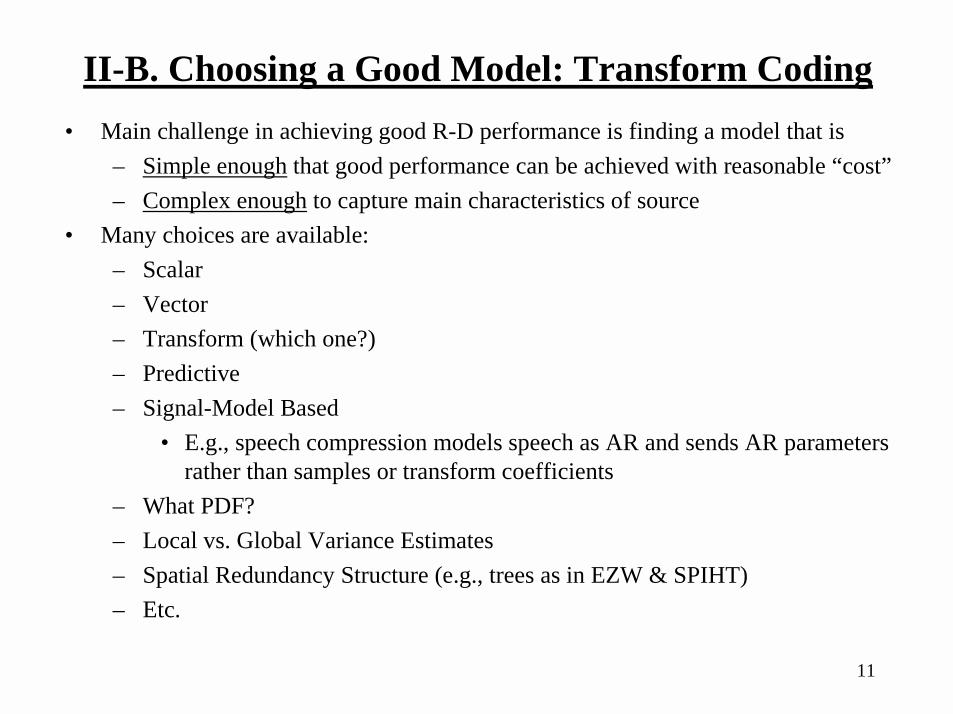
II-B. Choosing a Good Model: Transform Coding • Main challenge in achieving good R-D performance is finding a model that is

– Simple enough that good performance can be achieved with reasonable “cost”– Complex enough to capture main characteristics of source

• Many choices are available:– Scalar – Vector– Transform (which one?)– Predictive– Signal-Model Based

• E.g., speech compression models speech as AR and sends AR parameters rather than samples or transform coefficients

– What PDF?– Local vs. Global Variance Estimates– Spatial Redundancy Structure (e.g., trees as in EZW & SPIHT)– Etc.

12

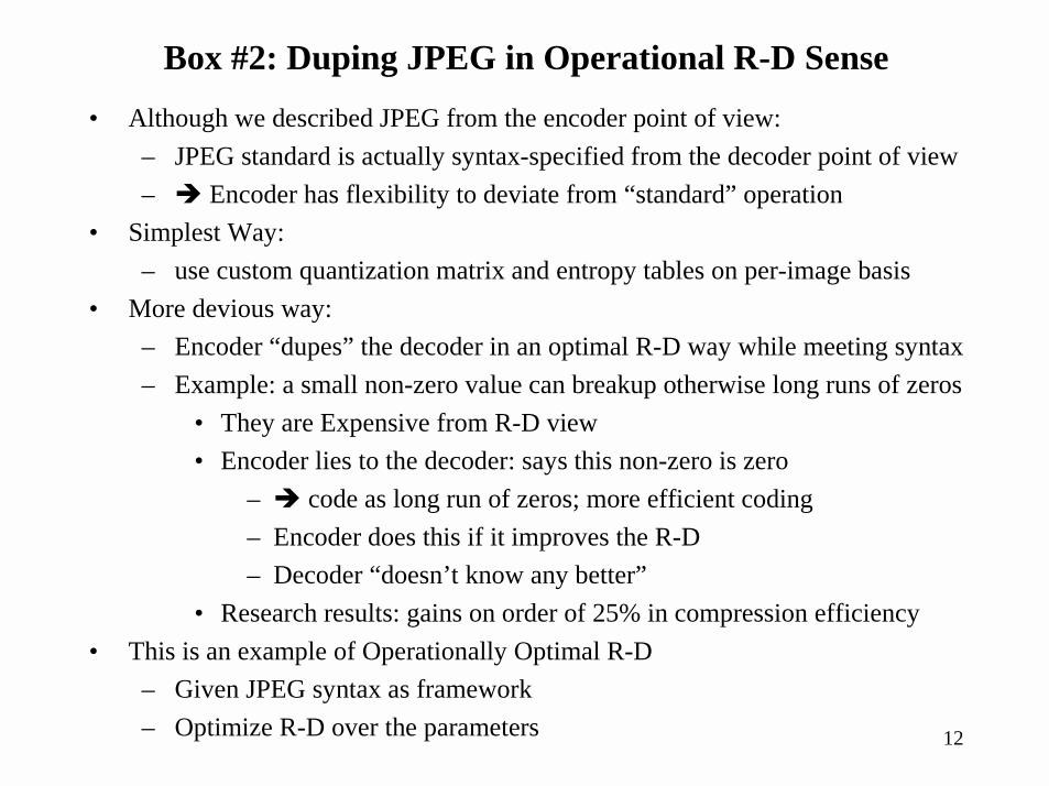
Box #2: Duping JPEG in Operational R-D Sense• Although we described JPEG from the encoder point of view:

– JPEG standard is actually syntax-specified from the decoder point of view– ! Encoder has flexibility to deviate from “standard” operation

• Simplest Way: – use custom quantization matrix and entropy tables on per-image basis

• More devious way:– Encoder “dupes” the decoder in an optimal R-D way while meeting syntax– Example: a small non-zero value can breakup otherwise long runs of zeros

• They are Expensive from R-D view• Encoder lies to the decoder: says this non-zero is zero

– ! code as long run of zeros; more efficient coding– Encoder does this if it improves the R-D– Decoder “doesn’t know any better”

• Research results: gains on order of 25% in compression efficiency• This is an example of Operationally Optimal R-D

– Given JPEG syntax as framework– Optimize R-D over the parameters

13

Box #3: Adaptive Transforms from Wavelets

• General transform coding framework:– Transform, quantizer, entropy coder– We’ve talked about encoder adapting quantizer and/or entropy coder

• i.e., via bit allocation– But, could also adapt the choice of transform

• Example: Wavelet is actually a family of flexible transforms – Adaptively choose a mother wavelet

• e.g. choose a particular filter from set of allowable wavelet filters– Adaptively choose the number of subbands used

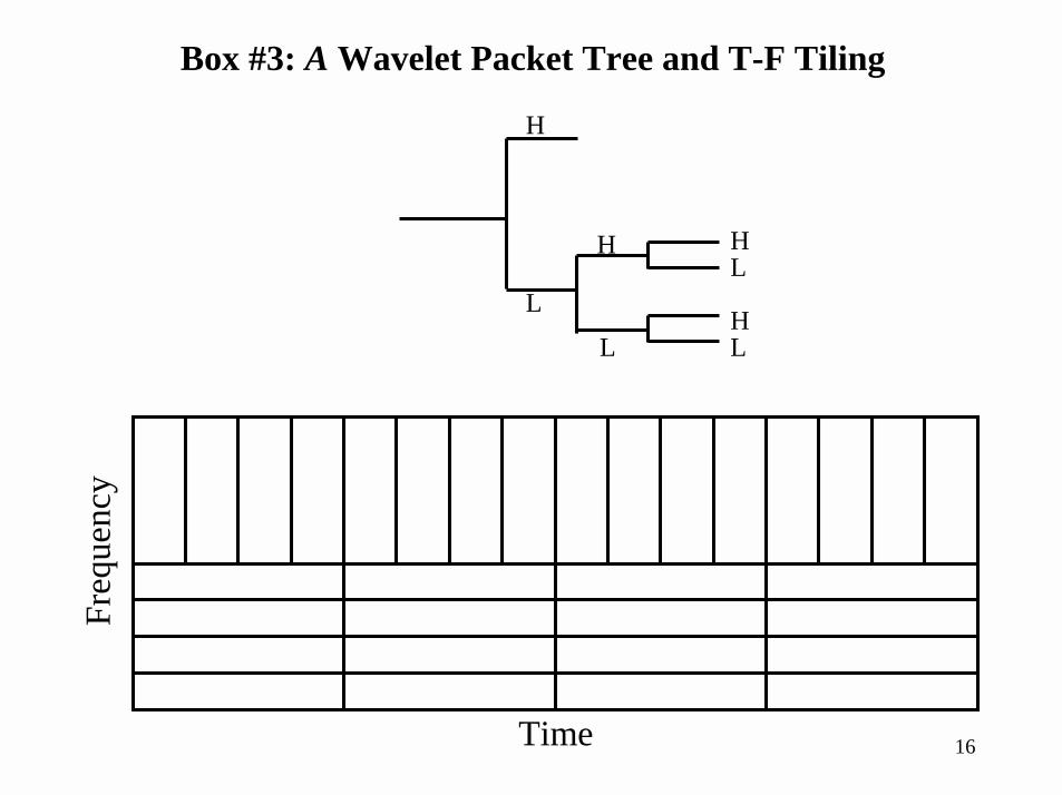
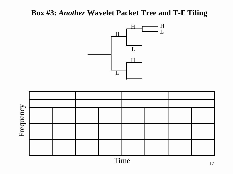
• Even more flexibility comes from generalizations of wavelets– Called wavelet packets– Come about from modifying wavelet filterbank structure

• Don’t always “leave HP channel, split LP channel”

14

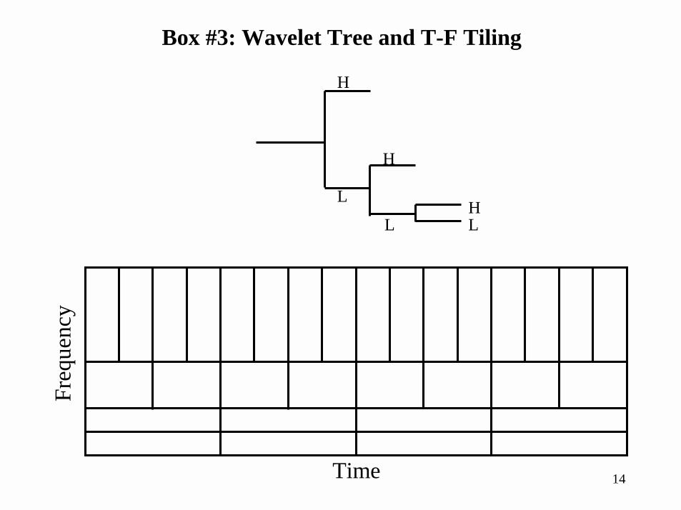
Box #3: Wavelet Tree and T-F Tiling

H

L

H

LHL

Time

Freq

uenc

y

15

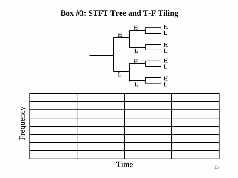
Box #3: STFT Tree and T-F Tiling

H

L

H

L

HL

H

L

HL

HL

HL

Time

Freq

uenc

y

16

Box #3: A Wavelet Packet Tree and T-F Tiling

L

H

L

H HL

HL

Time

Freq

uenc

y

17

Box #3: Another Wavelet Packet Tree and T-F TilingH

H

L

H

H

L

L

Time

Freq

uenc

y

18

II-C. Standards-Based Coding: Syntax-Constrained R-D Optimization

• Compression standards provide an agreed upon bit stream syntax– Needed to ensure interoperability– Any standard-compliant decoder can then decode bit stream

• Goal: Syntax-Constrained Optimization– Encoder’s task: select the best operating point from a discrete set of

options agreed upon a priori by a fixed decoding rule (i.e. the decoder syntax)

– Selected Operating Point is Side Information• Sent to decoder (typically in the header)• Trade-offs:

– Flexibility vs. Amount of Side Info– Flexibility vs. Computational Complexity

19

II-C. Standards-Based Coding (cont.)

• Note: optimizing for a particular input• Caution: selection of the coding framework is key to performance

– Bad Approach: poor framework & sophisticated optimization method– Recall Exp. #1 in Box #1: i.i.d. Gaussian & Shannon Coding = Bad

• Optimal Solution = the operating point giving best objective function value• Since there are finite number of operating points (coding choice)

– Could do an exhaustive search– But, strive for efficient non-brute-force optimization approach

Formulation #1 – General Discrete R-D Optimization:Given a specific encoding framework where the decoder is fully defined, optimize the encoding of a particular image or video sequence in order to meet some rate/distortion objectives

Formulation #1 – General Discrete R-D Optimization:Given a specific encoding framework where the decoder is fully defined, optimize the encoding of a particular image or video sequence in order to meet some rate/distortion objectives

20

Box #4: Delay Constrained Transmission & Buffer Control• Coding of Video Sequences results in a variable bit rate

– Need an Encoder Buffer to connect the variable bit rate (VBR) coded stream to the constant bit rate (CBR) channel

– Need Decoder Buffer to connect the CBR channel to the VBR decoding stream

• Video Input Rate = Video Output Rate ! constant ∆T (end-to-end delay)– Frame coded at time t must be decoded at time t + ∆T

EncoderBuffer

DecoderBuffer

CBRChannel

VideoEncoder

VideoDecoder

InputVideo

OutputVideo

∆Te ∆Teb ∆Tc ∆Tdb ∆Td

∆T

21

Box #4: Delay Constrained (Cont.)

• Encoder/Decoder Delays, ∆Te and ∆Td, assumed constant due to processing considerations

• Channel Delay, ∆Tc, is assumed constant because of CBR channel• Thus, only buffer delays, ∆Teb and ∆Tdb, are variable• Constraint on end-to-end delay ∆T ! Need for encoded rate control

– Constraint on ∆T puts an upper bound on buffer size Bmax (in bits)• Need Bmax< C ∆T where C = channel rate in bits/s• Otherwise bits going in when buffer is nearly full would take more

than ∆T to come out at the emptying rate of C– Range of Variation in Coded Rate puts lower limit on Bmax

• Otherwise we could overflow the buffer during high-rate segments– Thus we either have to:

• Use large buffers to deal with rate variation (causes excessive delay)• Use shorter buffers to meet delay and reduce variation using rate

control to ensure buffers don’t overflow• Note that MPEG (and other methods) have rate control capabilities

– Research Issue: Operational R-D Optimized Rate Control

22

III. Typical Allocation Problems• Two Basic Classes

– Compression for Storage• Rate Budget Constraint

– Compression for Transmission• Delay Constrained• Buffer Constrained

23

Several Practical Issues to Address

• Selection of Basic Coding Unit– Coding Unit = entity for which encoder parameters can be set

• Sample, Block, Image, Subsequence of Frames, Etc.– Example: Video

• Might use Coding Unit = Video Frame• Measure frame-wise rate-distortion & decide operating point per frame

– Example: Image• Might use Coding Unit = 8×8 block of pixels (JPEG)

– Optimization could be over a single coding unit or multiple units

• Complexity – Two main sources:– R-D itself may have to be measured from data (several encodes/decodes)

• Can ease this by using models or approximations of R-D– Finding the Optimal operating point

24

Several Practical Issues (Cont.)

• Cost Function – May include both rate and distortion– Easily computed for each coding unit– But, when allocating among several units:

• Overall cost requires careful definition• There are several options

– Example: Long Video Sequence• consider cost = average distortion over all units• Is this really a desirable cost function?

– Could have large peak distortion in some frames• Might it be better to minimize worst-case distortion?

– So-called minimax criterion– Could have larger average distortion

– Also should consider perceptually-weighted versions • Notation

– N coding units (i = 1, 2, …, N) Each having M operating points (j = 1, 2, ..

25

Notation

• Assume N coding units (i = 1, 2, …, N) • Each coding unit has M operating points (j = 1, 2, …, M)• For the ith coding unit when using the jth “quantizer” we have

– Rate: rij

– Distortion: dij

• “Quantizer” indices j are listed in order of increasing coarseness– j = 1 is the finest quantizer (highest rate, lowest distortion)– j = M is the coarsest quantizer (lowest rate, highest distortion)

• Will formulate problems under two types of constraint– Total Bit Budget (e.g., storage applications)– Transmission Delay (e.g., video transmission)

26

III-A. Storage Constraints: Budget-Constrained Allocation

• Here, rate is constrained by a restriction on the maximum total number of bits– Total Number of Bits = RT

– Must allocate the RT bits among the N coding units– Allocation should minimize some overall distortion metric

• Examples: – Allocate bits among 8×8 blocks of pixels in an image– Allocate bits among a set of images to be compressed into an archive

• Here we may care about the aggregate quality of the set of images

27

III-A. Budget-Constrained Allocation (Cont.)

• Example Metric: Minimum Average Distortion Metric (i.e., MMSE)

• Note: Formulation #3 with the Minimum Average Distortion Metric is nothing more than the bit allocation problem we already looked at– Where we assumed:

• Each quantizer’s input was i.i.d. with some known variance

Formulation #3 – Budget Constrained Allocation:Find the optimal quantizer (i.e., operating point) j(i) for each coding unit i such that

and some metric f (d1j(1), d2j(2), … , dNj(N)) is minimized.

Formulation #3 – Budget Constrained Allocation:Find the optimal quantizer (i.e., operating point) j(i) for each coding unit i such that

and some metric f (d1j(1), d2j(2), … , dNj(N)) is minimized.

∑=

≤N

iTiij Rr

1)(

∑=

=N

iiijNNjjj ddddf

1)()()2(2)1(1 ),,,( !

28

Alternative Metrics for Formulation #3

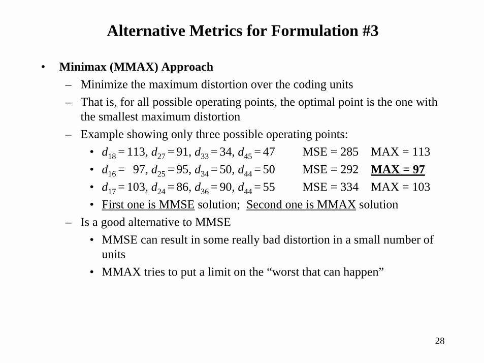
• Minimax (MMAX) Approach– Minimize the maximum distortion over the coding units– That is, for all possible operating points, the optimal point is the one with

the smallest maximum distortion– Example showing only three possible operating points:

• d18 = 113, d27 = 91, d33 = 34, d45 = 47 MSE = 285 MAX = 113• d16 = 97, d25 = 95, d34 = 50, d44 = 50 MSE = 292 MAX = 97• d17 = 103, d24 = 86, d36 = 90, d44 = 55 MSE = 334 MAX = 103• First one is MMSE solution; Second one is MMAX solution

– Is a good alternative to MMSE• MMSE can result in some really bad distortion in a small number of

units• MMAX tries to put a limit on the “worst that can happen”

29

Alternative Metrics for Formulation #3 (Cont.)

• Lexicographically Optimal (MLEX) Approach– Sort quantizers used into decreasing order of index (i.e. decreasing MSE)– Use sorted indices to form the digits of a number (one per operating point) – The optimal point is the one with the smallest such number– Example showing only three possible operating points (same as above):

• d18 = 113, d27 = 91, d33 = 34, d45 = 47 LEX = 8753 MSE = 285• d16 = 97, d25 = 95, d34 = 50, d44 = 50 LEX = 6544 MSE = 293• d17 = 103, d24 = 86, d36 = 90, d44 = 55 LEX = 7644 MSE = 334• Second one is MLEX solution

– MLEX is a generalization of MMAX– MLEX tends to equalize distortion across all coding units

• Gives the coded data a more uniform appearance

30

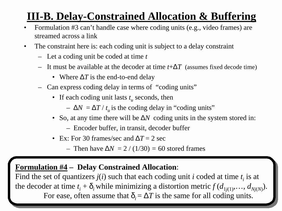
III-B. Delay-Constrained Allocation & Buffering • Formulation #3 can’t handle case where coding units (e.g., video frames) are

streamed across a link• The constraint here is: each coding unit is subject to a delay constraint

– Let a coding unit be coded at time t– It must be available at the decoder at time t+∆T (assumes fixed decode time)

• Where ∆T is the end-to-end delay– Can express coding delay in terms of “coding units”

• If each coding unit lasts tu seconds, then– ∆N = ∆T / tu is the coding delay in “coding units”

• So, at any time there will be ∆N coding units in the system stored in:– Encoder buffer, in transit, decoder buffer

• Ex: For 30 frames/sec and ∆T = 2 sec – Then have ∆N = 2 / (1/30) = 60 stored frames

Formulation #4 – Delay Constrained Allocation:Find the set of quantizers j(i) such that each coding unit i coded at time ti is at the decoder at time ti + δi while minimizing a distortion metric f (d1j(1),…, dNj(N)).

For ease, often assume that δi = ∆T is the same for all coding units.

Formulation #4 – Delay Constrained Allocation:Find the set of quantizers j(i) such that each coding unit i coded at time ti is at the decoder at time ti + δi while minimizing a distortion metric f (d1j(1),…, dNj(N)).

For ease, often assume that δi = ∆T is the same for all coding units.

31

• What impact does this delay constraint have on buffer constraints?– Assume a variable channel rate: C(i) bits/sec during the ith coding interval– Then encoder buffer state at time i is:

• B(i) = max [B(i-1) + rij(i) – C(i)] , 0 w/ initial state B(0) = 0• Also, B(i) can’t grow larger than buffer physical size: B(i) ≤ Bmax

• BUT, there is another constraint on the buffer:

Impact of Delay Constraint on Buffer

• • •B(i) B(i-1) B(i-2) B(i-3) B(i-4) B(i-K)

To ChannelC(i) bits/sec

Coded Frames

ith UnitThis must get out in ∆N coding units of delay

• How many bits can be emptied in ∆N coding units?

• Thus, to get the ith unit to the decoder in ∆T seconds using this channel there can be no more than Beff(i) bits in the buffer after the ith unit is put in the buffer

∑∆+

+==

Ni

ikeff kCiB

1)()(

32

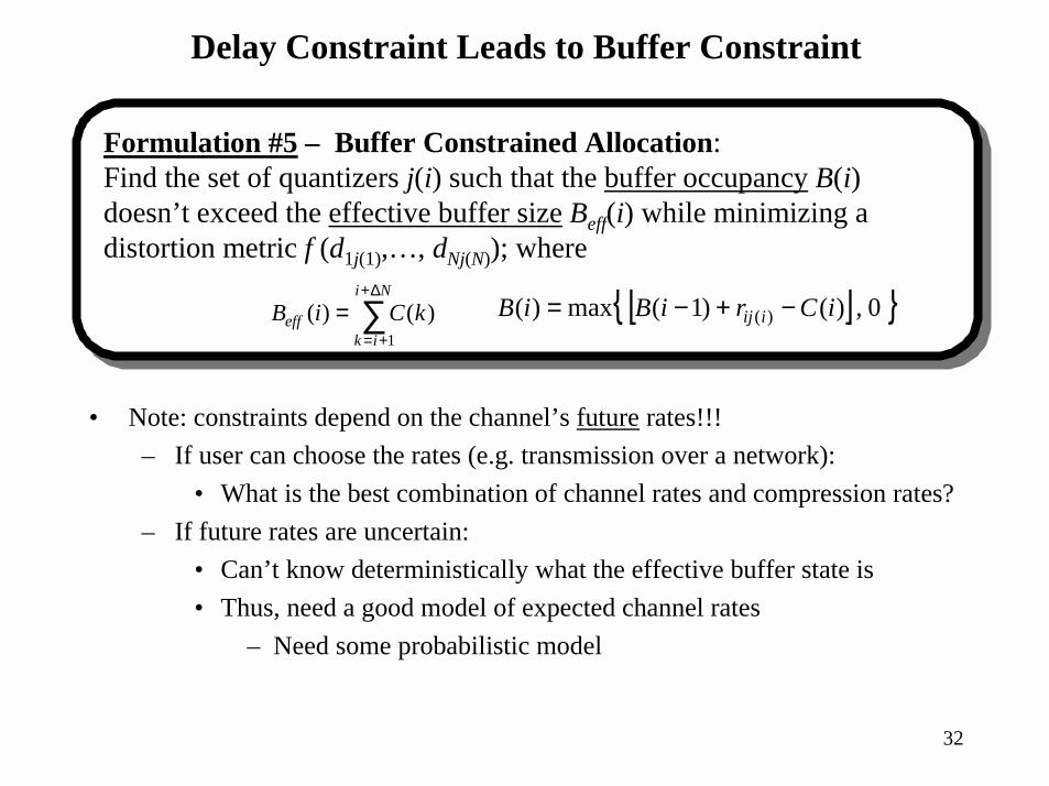
• Note: constraints depend on the channel’s future rates!!!– If user can choose the rates (e.g. transmission over a network):

• What is the best combination of channel rates and compression rates?– If future rates are uncertain:

• Can’t know deterministically what the effective buffer state is• Thus, need a good model of expected channel rates

– Need some probabilistic model

Delay Constraint Leads to Buffer Constraint

Formulation #5 – Buffer Constrained Allocation:Find the set of quantizers j(i) such that the buffer occupancy B(i) doesn’t exceed the effective buffer size Beff(i) while minimizing a distortion metric f (d1j(1),…, dNj(N)); where

Formulation #5 – Buffer Constrained Allocation:Find the set of quantizers j(i) such that the buffer occupancy B(i) doesn’t exceed the effective buffer size Beff(i) while minimizing a distortion metric f (d1j(1),…, dNj(N)); where

∑∆+

+==

Ni

ikeff kCiB

1)()( [ ] 0,)()1(max)( )( iCriBiB iij −+−=

33

IV. The R-D Optimization Toolbox• Two Types of Problems

– Independent Problems• R-D operating points can be

measured indep. for each coding unit– Dependent Problems

• R-D operating points for a coding unit depend on choices made for the others

34

IV-A. Independent Problems

• Here, rij and dij can be measured independently for each coding unit– Example: JPEG coding of AC DCT components; coding unit = block– Not Independent: anytime prediction between coding units is used

• Example: MPEG frames using motion-compensated prediction• Sometimes ignore dependence to speed up encoding

• Goal: Given some chosen coding framework: – Compute or obtain the achievable R-D operating point data– Use some optimization method to choose the optimal operating point

according to some appropriate formulation• Two main optimization methods discussed:

– Lagrangian• Operational form of “equal slope” solution we discussed earlier

– Dynamic Programming• Trellis-based solution (similar to Viterbi Algorithm in digital comm.)

35

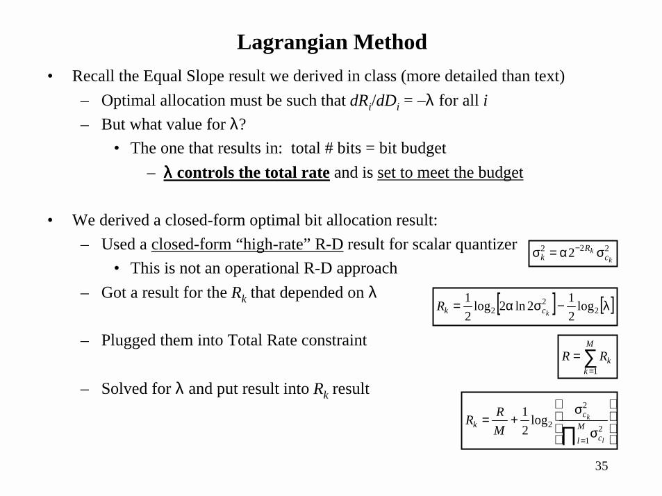
Lagrangian Method• Recall the Equal Slope result we derived in class (more detailed than text)

– Optimal allocation must be such that dRi/dDi = –λ for all i– But what value for λ?

• The one that results in: total # bits = bit budget– λλλλ controls the total rate and is set to meet the budget

• We derived a closed-form optimal bit allocation result: – Used a closed-form “high-rate” R-D result for scalar quantizer

• This is not an operational R-D approach– Got a result for the Rk that depended on λ

– Plugged them into Total Rate constraint

– Solved for λ and put result into Rk result

σ

σ+=

∏ =

M

l c

ck

l

k

MRR

12

2

2log21

[ ] [ ]λ−σα= 22

2 log212ln2log

21

kckR

222 2k

kc

Rk σα=σ −

∑=

=M

kkRR

1

36

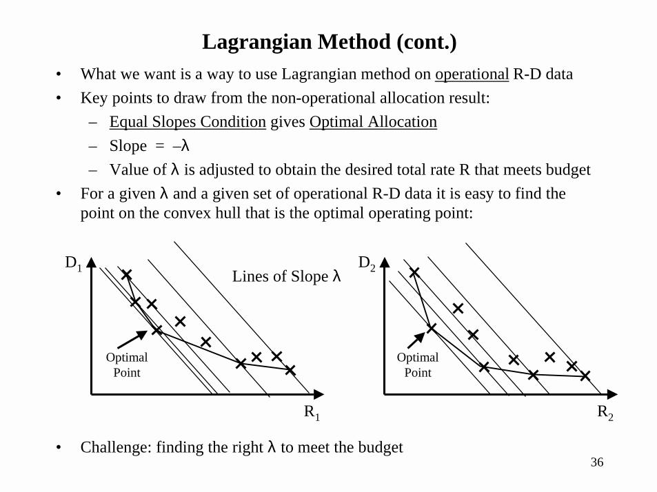
• What we want is a way to use Lagrangian method on operational R-D data• Key points to draw from the non-operational allocation result:

– Equal Slopes Condition gives Optimal Allocation– Slope = –λ– Value of λ is adjusted to obtain the desired total rate R that meets budget

• For a given λ and a given set of operational R-D data it is easy to find the point on the convex hull that is the optimal operating point:

Lagrangian Method (cont.)

R2

D2

R1

D1 Lines of Slope λ

OptimalPoint

OptimalPoint

• Challenge: finding the right λ to meet the budget

37

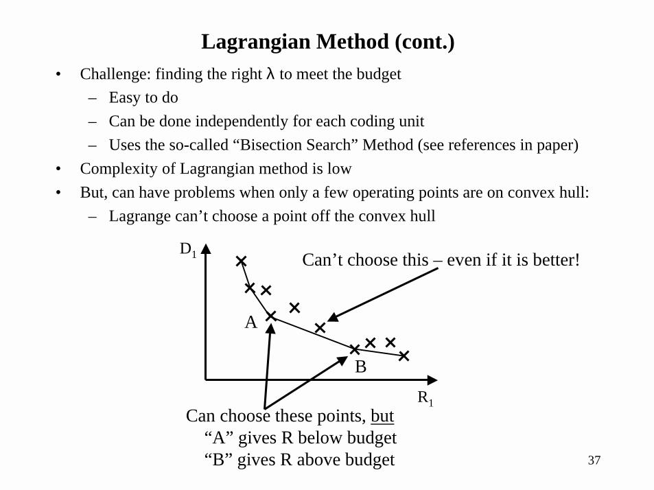
• Challenge: finding the right λ to meet the budget– Easy to do– Can be done independently for each coding unit– Uses the so-called “Bisection Search” Method (see references in paper)

• Complexity of Lagrangian method is low• But, can have problems when only a few operating points are on convex hull:

– Lagrange can’t choose a point off the convex hull

Lagrangian Method (cont.)

R1

D1

Can choose these points, but“A” gives R below budget“B” gives R above budget

Can’t choose this – even if it is better!

A

B

38

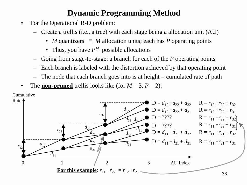
• For the Operational R-D problem:– Create a trellis (i.e., a tree) with each stage being a allocation unit (AU)

• M quantizers ≡ M allocation units; each has P operating points• Thus, you have PM possible allocations

– Going from stage-to-stage: a branch for each of the P operating points– Each branch is labeled with the distortion achieved by that operating point– The node that each branch goes into is at height = cumulated rate of path

• The non-pruned trellis looks like (for M = 3, P = 2):

Dynamic Programming Method

0 1 2 3 AU Index

CumulativeRate

d11

d12 d21

d22

d21

d22

d31

d32

d31

d32d31

d32

D = d11 +d21 + d31

D = d11 +d21 + d32

D = ????D = ????D = d12 +d22 + d31

D = d12 +d22 + d32

r22

r32

r12

R = r11 +r21 + r31

R = r11 +r21 + r32

R = r12 +r22 + r31

R = r12 +r22 + r32

R = r11 +r22 + r31

R = r11 +r22 + r32

For this example: r11 +r22 = r12 +r21

39

• Prune the trellis as it is built– Prune it to optimize– Prune it when it exceeds a constraint

• Pruning to optimize– If two branches go to the same node (i.e. have the same cumulative rate)

• Prune the one with the larger distortion• Retains minimum distortion for that node

– This is Bellman’s Optimality Principle » a.k.a. Viterbi Algorithm» a.k.a. Dykstra’s Algorithm

Dynamic Programming Method (cont.)

0 1 2 AU Index

CumulativeRate

d11

d12 d21

d22

d21

d22Assume for example: d12 +d21 > d11 +d22

Prune the dashed branch

40

• Pruning to meet constraints– Prune a branch if it exceeds the Total Rate Constraint (Bit Budget)

• Trellis can’t grow above a “ceiling”– Prune a branch it it exceeds the Buffer Constraint

• Would need to keep track of Buffer Size of Each Branch– On each branch, put a second “tag” along side its distortion tag

• Con: Computationally Complex• Pro: Method can achieve operating points that are not on convex hull• When points are dense on convex hull Lagrangian method can give nearly as

good result at much less complexity

Dynamic Programming Method (cont.)

0 1 2 3 AU Index

CumulativeRate

d11

d12 d21

d22

d21

d31

d32

d31

d32d31

d32

Bit Budget

D = d11 +d21 + d31

D = d11 +d21 + d32

D = d11 +d22 + d31 d22Pick TheOne WithSmallest D

41

IV-B. Dependent Problems• In some scenarios we can’t make decisions independently on each coding unit• One example of this is in predictive-based coding:

– Assume that the ith coding unit is predicted from the (i-1)th coding unit– Prediction is done using the past quantized data

• Must use quantized data since that is what the decoder has available– Otherwise there is a growth in the quantization error variance– See equation (10.8) in textbook

• But this use of quantized data causes a dependency between coding units when you try to find the optimal operating points

• To see how this works we first need to revisit the Lagrangian cost

42

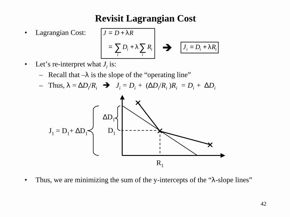
Revisit Lagrangian Cost• Lagrangian Cost:

• Let’s re-interpret what Ji is:– Recall that –λ is the slope of the “operating line”– Thus, λ = ∆Di/Ri ! Ji = Di + (∆Di/Ri )Ri = Di + ∆Di

• Thus, we are minimizing the sum of the y-intercepts of the “λ-slope lines”

∑∑ λ+=

λ+=

ii

ii RD

RDJ

iii RDJ λ+=

R1

D1

∆D1

J1 = D1+ ∆D1

!

43

Dependency Between Coding Units• Consider this simple video example of two frames:

– Assume each frame can be coded at 3 different quantizer settings– 1st frame is an independent frame (e.g., an “I” frame in MPEG)

• Thus, there are only 3 R-D operating points– 2nd frame is a dependent frame (e.g., a “P” frame in MPEG)

• Thus, there are 9 R-D operating pointso There are 3 points for each possible point used for 1st frame

R1

D1

R2

D2

1,1

1,2

1,3

2,1

2,2

2,3

3,1

3,2

3,3

1

2

3

44

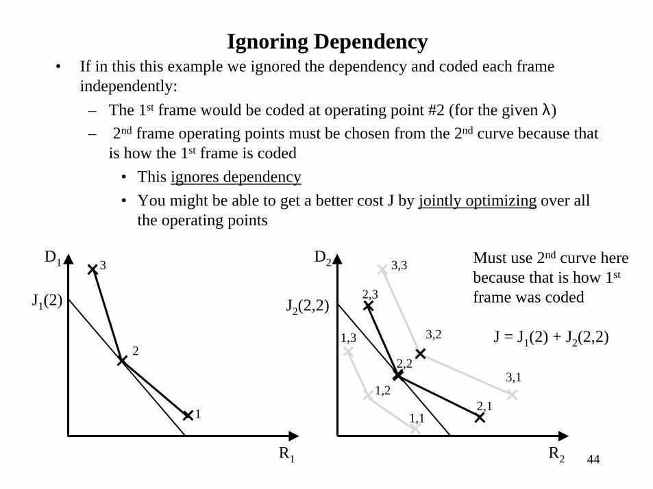
Ignoring Dependency• If in this this example we ignored the dependency and coded each frame

independently:– The 1st frame would be coded at operating point #2 (for the given λ)– 2nd frame operating points must be chosen from the 2nd curve because that

is how the 1st frame is coded• This ignores dependency• You might be able to get a better cost J by jointly optimizing over all

the operating points

R1

D1

R2

D2

1,22,1

2,2

2,3

3,1

3,2

3,3

J1(2) J2(2,2)

Must use 2nd curve herebecause that is how 1st

frame was coded

J = J1(2) + J2(2,2)2

3

1 1,1

1,3

45

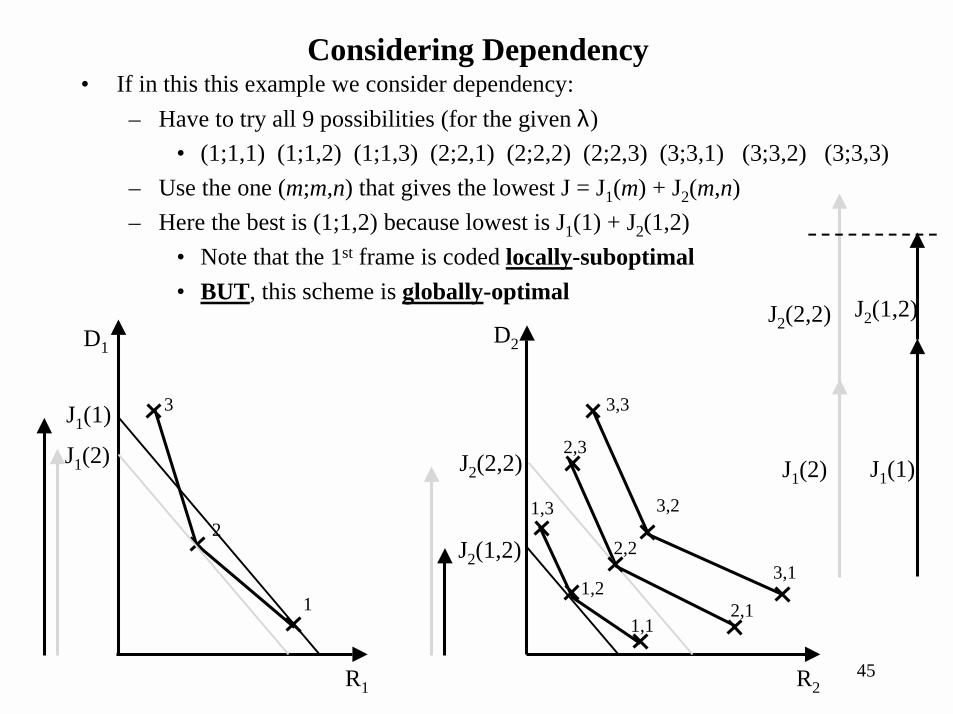
Considering Dependency• If in this this example we consider dependency:

– Have to try all 9 possibilities (for the given λ)• (1;1,1) (1;1,2) (1;1,3) (2;2,1) (2;2,2) (2;2,3) (3;3,1) (3;3,2) (3;3,3)

– Use the one (m;m,n) that gives the lowest J = J1(m) + J2(m,n)– Here the best is (1;1,2) because lowest is J1(1) + J2(1,2)

• Note that the 1st frame is coded locally-suboptimal• BUT, this scheme is globally-optimal

R1

D1

1

2

3

R2

D2

2,1

2,2

2,3

3,1

3,2

3,3

J1(2) J2(2,2)

J1(1)

1,1

1,2

1,3

J2(1,2)

J1(2)

J2(2,2)

J1(1)

J2(1,2)

46

Handling Dependency

• Complicates the computing of the R-D operating points– Can sometimes use analytic models of the dependent R-D characteristics

• Then don’t need to compute all possible operating R-D values• Necessitates the use of dynamic programming

– Use trellis-based approaches that capture the dependence• Full trellis structure has exponential growth in number of combinations

– Possible to make approximations that simplify the search– Possible to embed suboptimal approaches into the trellis

• Prune at each stage use e semi-greedy approach

47

V. Application to Basic Components in Image/Video Coding Algorithms• Budget Constraint Problems

– Fixed-Transform-Based Case– Adaptive Transform-Based Case

• Delay Constraint Problems• Role of R-D in Joint Source-Channel Coding

This section of the paper gives a tour of the types of problems that have been addressed in the recent literature and gives thorough pointers to relevant, high-quality references.

This section of the paper gives a tour of the types of problems that have been addressed in the recent literature and gives thorough pointers to relevant, high-quality references.