notes on theory and numerical methods for hyperbolic ...putti/teaching/dottorato/hyper.pdf · notes...
TRANSCRIPT

Notes on theory and numerical methods for hyperbolicconservation laws
Mario PuttiDepartment of Mathematics – University of Padua, Italy
e-mail: [email protected]
January 19, 2017
Contents1 Partial differential equations 2
1.1 Mathematical preliminaries and notations . 31.1.1 The chain rule of differentation . . 61.1.2 Integration by parts . . . . . . . . . 6
1.2 Classification of the PDEs . . . . . . . . . 71.2.1 Standard classification of linear PDEs 91.2.2 Simple examples and solutions . . . 111.2.3 Conservation laws . . . . . . . . . 15
1.3 Well posedness and continuous dependenceof solutions on the data . . . . . . . . . . . 161.3.1 Ill-conditioning and instability . . . 18
2 Hyperbolic Equations 212.1 Some examples . . . . . . . . . . . . . . . 21
2.1.1 The transport equation . . . . . . . 222.1.2 The second-order wave equation . . 232.1.3 Simple finite difference discretization 24
2.2 The method of characteristics . . . . . . . . 322.3 Initial-Boundary value problems . . . . . . 392.4 Classification of PDEs and propagation of
discontinuities . . . . . . . . . . . . . . . . 462.4.1 Propagation of singularities . . . . 47
2.5 Linear second order equations . . . . . . . 482.6 Systems of first-order equations . . . . . . 50
2.6.1 The linear case . . . . . . . . . . . 502.6.2 The quasi-linear case . . . . . . . . 54
2.7 Weak solutions for conservation laws . . . . 552.7.1 Jump conditions . . . . . . . . . . 58
2.7.2 Admissibility conditions . . . . . . 612.8 The Riemann Problem. . . . . . . . . . . . 65
2.8.1 Shock and rarefaction curves . . . . 69
3 Numerical Solution of Hyperbolic ConservationLaws 733.1 The Differential Equation . . . . . . . . . . 743.2 The Finite Volume Method . . . . . . . . . 74
3.2.1 Preliminaries . . . . . . . . . . . . 743.2.2 Notations . . . . . . . . . . . . . . 77
3.3 The numerical flux. . . . . . . . . . . . . . 783.3.1 One spatial dimension: first order . 783.3.2 One spatial dimension: second or-
der gradient reconstruction . . . . . 82
A Finite Difference Approximations of first andsecond derivatives in R1. 85
B Fortran program: Godunov method for Burgersequation 87
C Memorization of 2D Computational Meshes. 100
D Review of linear algebra 101D.1 Vector spaces, linear independence, basis . 105
D.1.1 Orthogonality . . . . . . . . . . . . 107D.2 Projection Operators. . . . . . . . . . . . . 108D.3 Eigenvalues and Eigenvectors . . . . . . . . 112D.4 Norms of Vectors and Matrices . . . . . . . 115D.5 Quadratic Forms . . . . . . . . . . . . . . 118D.6 Symmetric case A = AT . . . . . . . . . . 123
1
These notes are a free elaboration from [7, 1, 2] and other sources.
1 Partial differential equationsIn this notes we will look at the numerical solution for partial differential equations. We will bemainly concerned with differential models stemming from conservation laws, such as those arisingfrom force conservations i.e., second Newton’s law F = ma, such as de Saint-Venant equations,governing the equilibrium of a solid, or the Navier-Stokes equations, governing the dynamics of fluidflow. These equations are also called “equations in divergence form”, to identify the fact that thedivergence of a vector translates in mathematical terms the conservation of the flux represented bythat vector field.As an example, let us consider the advection-diffusion equation (ADE), that governs the conservationof mass of a solute moving within the flow of the containing solvent. A typical application is thetransport of a contaminant by a water body moving with laminar flow. The flow of the solvent isgiven by the vector (velocity) field λ, and the solute is undergoing chemical (Fickian) diffusion witha diffusion field D(x). We remark that if the density of the solvent is constant, then mass conserva-tion is equivalent to volume concentration, and thus density does not appear in the equations. Themathematical model is then given by:
∂u
∂t= div (D∇u)− div(λu) + f in Ω ∈ Rd (1.1)
where the equation is defined on a subspace of the d-dimensional Euclidean space Rd (d = 1, 2, or3), the function u(x, t) : Ω× [0 : T ] 7→ R represents the concentration of the solute (mass/volume ofsolute per unit mass/volume of solvent), t is time, div =
∑i ∂/∂xi is the divergence operator, D is
the diffusion coefficient, possibly a second order tensor, and∇ = ∂/∂xi is the gradient operator. Aproblem is mathematically well posed if i) it has a solution; ii) the solution is unique; iii) the solutiondepends continuously on the data of the problem. For a PDE problem to be well-posed we needinitial and boundary conditions. So we let the domain boundary Γ = ∂Ω be the union of three nonoverlapping sub-boundaries such that Ω = ΓD ∪ ΓN ∪ ΓC , so that we:
u(x, 0) = uo(x) x ∈ Ω, t = 0 (initial conditions) (1.2a)u(x, t) = gD(x) x ∈ ΓD, t > 0 (Dirichlet BCs) (1.2b)
−D∇u(x, t) · ν = qN(x) x ∈ ΓN , t > 0 (Neumann BCs) (1.2c)λu−D∇u(x, t) · ν = qC(x) x ∈ ΓC , t > 0 (Cauchy BCs) (1.2d)
where ν is the outward unit normal defined on Γ. Formally, under some regularity assumption andthe hypothesis that D never vanishes, this is called a “parabolic” equation. The term “parabolic” isused to classify partial differential equations (PDEs) on the basis of certain qualitative properties ofthe solution. This can be done relatively easily with linear PDEs, and becomes more complicated fornonlinear PDEs.
2
1.1 Mathematical preliminaries and notationsWe start this discussion by giving some general definitions. All our objects or equations will bedefined in a domain Ω ⊂ Rd, and we will indicate with x ∈ Ω a point of the d-dimensional space(d=1, 2, or 3) as a vector with d coordinates x = (x1, x2, . . . , xd)
T with respect to a fixed Cartesian(orthonormal) reference system. 1 Note that, for simplicity, we assume vectors to be 1-dimensionalcollections of numbers ordered columnwise, and will use the transpose operation as above to indicatea row vector (see appendix D). If d = 2 we will often identify x = x1 and y = x2. A function u(x)is a spatially-variable real-valued scalar function taking values in Ω ⊂ Rd and returning real valuesin R. A vector-valued function q(x) is a collection of functions ordered in a column vector. Thus wehave:
u : Ω 7→ R q : Ω 7→ Rm; q(x) =
q1(x)...
qm(x)
.
Typically, physical quantities such as fluxes, velocities, etc. are defined in Rd, i.e., in the above wehave m = d.
Definition 1.1 (Derivatives). 1. first order partial derivative:
uxi =∂u(x)
∂xi= lim
h→0
u(x+ hei)− u(x)
h
where ei is the i-th coordinate vector, i.e., the vector with the i-th component equal to one andall the other ones equal to zero.
2. second order partial derivatives:
uxixj =∂2u(x)
∂xi∂xj,
with obvious extensions for higher order.
3. Multiindex Notation.
(a) Given a vector α = (α1, . . . , αd)T , where αi ≥ 0 (the multi-index of order | α |= α1 +
. . .+ αd), the α-th derivative is:
∇α u(x) :=∂|α|u(x)
∂xα11 · · · ∂xαdd
= ∂α1x1· · · ∂αdxd .
1We would like to remark that formally Ω is an open subset of Rd, and its closure is indicated with Ω = Ω d Γ, whereΓ = ∂Ω is the boundary of Ω, which forms a subset of Rd of co-dimension 1, i.e., d − 1 (for d = 2 the boundary is acurve, for d = 3 it is a surface). We will not use or make reference to these technicalities, as empirical intuition can besufficiently supported without them.
3

(b) if k is a nonnegative integer, then the set of all partial derivatives of order k is given by:
∇k u(x) := ∇α u(x) :| α |= k .
Giving an order to the partial derivatives of the set above, we can think of ∇k u(x) as apoint (vector) in Rdk , and we can define the length of this point as:
| ∇k u(x) |=
∑|α|=k
| ∇α u |2 1
2
.
(c) Special cases. If k = 1 we order the elements of ∇u in a vector thus leading to thedefinition of the “gradient” operator:
∇u :=
ux1...uxd
Thus we can regard∇u as a point of Rd.
4. The divergence of a vector function q(x) : Ω ⊂ Rd 7→ Rd as:
div q(x) := ∇ ·q(x) = ∇T q(x) =∂q1(x)
∂xi+ . . .
∂qd(x)
∂xd
For example, for d = 2 we have:
∇u(x) =
(ux1ux2
)=
( ∂u∂x1∂u∂x2
)div q(x) = ∇ ·q(x) =
∂q1(x)
∂x1
+∂q2(x)
∂x2
We would like to stress here that we will generally see the gradient as an operator acting ona scalar-valued function and the divergence as an operator acting on a vector-valued function.Note that the divergence and the gradient operators are intimately related by the divergence (orGauss’ or Stokes) theorem, which we will discuss later on.
5. For k = 2 we organize the elements of∇2 u(x) in a matrix, called the Hessian matrix:
∇2 u(x) = ∇∇T u(x) =
ux1x1 · · · ux1xd. . .
uxdx1 · · · uxdxd
Unfortunately, the symbol ∇2 should not be confused with the Laplacian operator, often indi-cated by∇2.
4
6. Laplacian operator: The Laplacian operator is given by:
∆u(x) = div∇u(x) = ∇T ∇u(x) = Tr(∇2 u(x)
)=
d∑i=1
uxixi .
where the operator Tr (A) is the trace of a matrix A (see appendix D).
Definition 1.2 (Partial differential equation). A k-th order partial differential equation (PDE) can bewritten as:
F (x, u(x),∇u(x),∇2 u(x), . . . ,∇k u(x)) = 0, x ∈ Ω. (1.3)
where formally F : Ω×R×Rd . . .×Rdk−1 ×Rdk 7→ R. For example, for k = 2 and d = 3 we have:
F (x, y, z, u, ux, uy, uz, uxx, uxy, uyy, uxz, uzz, uyz) = 0.
The solution of this equation is a function u(x) : Ω ⊂ Rd 7→ R that satisfies eq. (1.3) and possiblysome other boundary conditions.
The problem we are concerned with is finding solutions (either approximate or exact) to eq. (1.3). IfF is a linear function of u and its derivatives, then the equation is called linear, and, assuming d = 2,it can be written as:
a(x, y) + b(x, y)u+ c(x, y)ux + d(x, y)uy + e(x, y)uxx + f(x, y)uyy + g(x, y)uxy = 0. (1.4)
The order of a PDE is the order of the derivative of maximum degree that appears in the equation.Thus, in the previous case the order is 2. Typical examples are:
∆u =∂2u
∂x2+∂2u
∂y2= 0 2o order (Laplace equation)
∂u
∂t+∂u
∂x= 0 1o order (transport or convection equation)
∂u
∂t− ∂2u
∂x2= 0 2o order (diffusion equation).
Note that we often identify one of the variables as time, in which case, setting xd+1 = t, the solutionu has domain given by Ω× [0, T ]:
u : Ω× [0, T ] 7→ R.
Obviously, we consider time as a positive real number.
5
1.1.1 The chain rule of differentation
We say that a function u(x) is smooth when it is infinitely differentiable, i.e., u(x) ∈ C∞(Ω). We willbe using often the chain (product) rule of differentiation and its derived property, i.e., integration byparts. For d = 1, using u′ to indicate differentation, we can write:
(uv)′ = u′v + uv′ (1.5)
which is valid for all u and v in C∞. By extension, we can think that the derivative of a scalar valuedfunction in Ω as the gradient operator, i.e., the collection of all its partial derivatives. The chain ruleis then:
∇(uv) = u∇ v + v∇u. (1.6)
If we have a scalar function u : Ω 7→ R and a vector-valued function q : Ω 7→ Rd, we may form theproduct qu = (q1u, . . . , qdu). Applying eqs. (1.5) and (1.6) component by component, we obtain:
div(qu) = q · ∇u+ u div q. (1.7)
Note that this is a straight forward extension if we think that the gradient acts on scalar functions, andthe divergence acts on vector functions.
1.1.2 Integration by parts
Recall the rule of integration by parts. It can be derived quickly from the chain rule. For d = 1, infact, using eq. (1.5), we can write:∫ b
a
u′(x)v(x) dx =
∫ b
a
(u(x)v(x)
)′dx−
∫ b
a
u(x)v′(x) dx
=(u(b)v(b)− u(a)v(a)
)−∫ b
a
u(x)v′(x) dx (1.8a)
In words, integration by parts states that the integral of the product of two functions (here u′(x) andv(x)) is equal to the product of the primitive of the first function multiplied by the other functionevaluated at the extremes, minus the integral of the primitive times the derivative.These results are easily extended in the multidimensional case. In this case, it is easy2 to rememberall these results by using the above definitions of gradient and divergence as vector operators. Recallagain that the gradient acts on scalars and the divergence acts on vectors. We recall here the importantGauss’ (or Divergence) Theorem that states a conservation principle:∫
Ω
div q(x) dx =
∫Γ
q(x) · ν(x) dx,
2at least for me
6

where the vector ν(x) is the outward unit normal defined on the boundary Γ of Ω. We can now statethe theorem of multidimensional integration by parts (or second Green’s Lemma) by recasting theone-dimensional integration by parts in the proper setting. Thus Green’s Lemma states that:∫
Ω
u(x) div q(x) dx =
∫Γ
u(x)q(x) · ν(x) dx−∫
Ω
∇u(x) · q(x) dx. (1.9)
To make the parallelism with the one-dimensional analogue, which helps remembering the theorem,we first look at eq. (1.8a). We observe that the term u(b)v(b) − u(a)v(a) can be interpreted as aboundary integral once we note that the “normal” in x = a is ν(a) = −1 and the “normal” in x = b isν(b) = +1, and the “zero”-dimensional integral is just the evaluation of the integrand at the extremesof integration. Looking at eq. (1.9) we can see that q(x) can be interpreted as the primitive of div q(x)and ∇u(x) as the (multiindex) first derivative of u(x). Then we can put Green’s Lemma in words:the integral of the product of two functions is given by the d− 1-dimensional integral of the productbetween the primitive of one of the two functions times the other one, everything projected along theoutward unit normal to the d − 1-dimensional boundary of the domain, minus the integral over thedomain of the product of the primitive function times the derivative of the other function.We would like to stress here that we have assumed that the functions are infinitely differentiable. Thisis too strong an assumption, and we could have assumed that first derivatives of the functions existand are finite for all x. This means that u and qi must be continuous functions of x (must be in C0(Ω)).In the case they are not, we need to be careful in applying the chain rule. Moreover, numerically thechain rule is troublesome, and should be avoided. We will discuss this in later sections.
1.2 Classification of the PDEsWe first start our classification by looking at the “linearity” of the function F in eq. (1.3). We say thata PDE is linear if all the derivatives appear as linear combinations, i.e. if it has the form:
a0(x)u+ a1(x)∇u+ . . .+ ak(x)∇k u =∑|α|≤k
aα(x)∇α u = f(x)
If f = 0 the PDE is called homogeneous. A PDE is semilinear if only derivatives of order strictlysmaller than k appear as nonlinear terms:∑
|α|=k
aα(x)∇α u+ a0
(∇k−1, . . . ,∇k u, u, x
)= 0.
It is called quasilinear if the highest order derivatives are multiplied by functions of strictly lowerorder derivatives:∑
|α|=k
aα
(∇k−1, . . . ,∇k u, u, x
)∇α u+ a0
(∇k−1, . . . ,∇k u, u, x
)= 0.
and it is fully nonlinear if the highest order derivatives appear nonlinearly in the equations.
7
Examples.
Laplace Equation
div∇u = ∆u = uxx + uyy = 0
This is an ubiquitous linear equation whose solution u is called potential function or harmonicfunction. In two dimensions, we can associate to a harmonic function u(x, y) a “conjugate”harmonic function v(x, y) such that the Cauchy-Riemann equations are satisfied:
ux = vy uy = −vx
We can interpret the vector field (u(x, y),−v(x, y) as the velocity of an irrotational and incom-pressible fluid.
Wave equation
utt = λ2∆u
Again, this is a ubiquitous linear equation that governs the vibration of a string or the propaga-tion of waves in an incompressible medium (e.g., fluid waves, sound).
Maxwell equation
εEt = curlH; µHt = − curlE; divE = divH = 0
where E = (E1, E2, E3) and H = (H1, H2, H3) are the electric and magnetic vector fields,respectively, in vacuum. Note that each component, Ej and Hj of E and H satisfy a waveequation with λ2 = 1/εµ.
Linear Elastic waves
ρutt = µ∆u+ (λ+ µ)∇(div u),
where ρ is the density of the medium, u = ui(x, y, z, t) represents the displacement vector,and λ and µ are the Lame constants. Each component ui of u satisfies a fourth order linearequation:(
∂2
∂t2− λ+ 2µ
ρ∆
)(∂2
∂t2− µ
ρ∆
)ui = 0
It is easy to see that in the case of equilibrium (ut = 0) this equation reduces to the bi-harmonicequation:
∆2u = 0.
8

σ
FIGURE 1.1: Curve γ and local reference system
Minimal surface We want to find a surface z = u(x, y) with minimal area for a given contour. Thefunction u satisfies the nonlinear equation:
(1 + u2y)uxx − 2uxuyuxy + (1 + u2
x)uyy = 0.
Navier-Stokes
ut + u · ∇u = −1
p∇ p+ ν∆u
div u = 0
where u(x, y, z, t) is the velocity, p(x, y, z, t) is the pressure, ρ is the density and ν is thekinematic viscosity of the fluid. These nonlinear equations govern the movement of an incom-pressible viscous fluid.
1.2.1 Standard classification of linear PDEs
To start in our task of classification, assume for simplicity a 2-dimensional domain d = 2, and aconstant coefficient second order PDE:
auxx + buxy + cuyy + e = 0. (1.10)
We look for a curve γ : R2 7→ R that is sufficiently regular and such that when we write the PDE alongthis curve it turns into and Ordinary Differential Equation (ODE). We write this curve in parametricform as γ(σ) (fig. 1.1) as follows:
γ =
x = x(σ)y = y(σ)
Writing the above equations on a local reference system, we obtain:
duxdσ
=∂ux∂x
dx
dσ+∂ux∂y
dy
dσ= uxx
dx
dσ+ uxy
dy
dσduydσ
=∂uy∂x
dx
dσ+∂uy∂y
dy
dσ= uxy
dx
dσ+ uyy
dy
dσ.
Writing uxx from the previous system and substituting it in eq. (1.10), we have:
uxy
[a
(dy
dx
)2
− bdydx
+ c
]−(aduxdx
dy
dx+ c
duydx
+ edy
dx
)= 0.
9

This equation is a re-definition of the PDE on the curve γ(σ), or, in other words, the equation issatisfied on γ. Now we can choose γ so that the first term in square brackets is zero, obtaining anequation for ux and uy where only ordinary derivatives appear:
a
(dy
dx
)2
− bdydx
+ c = 0.
We note that dy/dx is the slope of γ, which can then be obtained by solving the ODE:
dy
dx=b±√b2 − 4ac
2a. (1.11)
The solution of this ODE yields families of curves, that are called characteristic curves. Differentfamilies arise depending on the sign of the discriminant ∆ = b2 − 4ac. We then call the equationsdepending on this sign, obtaining the following classification:
• b2 − 4ac < 0: two complex solutions: the equation is “elliptic”;
• b2 − 4ac = 0: one real solution: the equation is “parabolic”;
• b2 − 4ac > 0: two real solutions: the equation is “hyperbolic”.
Examples
Laplace equation
∆u =∂2u
∂x2+∂2u
∂y2= 0
a = c = 1 b = 0 7→ b2 − 4ac < 0 is an elliptic equation;
Wave equation
∂2u
∂t2− ∂2u
∂x2= 0 (1.12)
a = 1 b = 0 c = −1 7→ b2 − 4ac > 0 is a hyperbolic equation;
diffusion or heat equation
∂u
∂t− ∂2u
∂x2= 0
a = −1 b = c = 0 7→ b2 − 4ac = 0 is a parabolic equation.
10

1.2.2 Simple examples and solutions
We show in this paragraph some simple but clarifying examples of PDEs and their exact analyticalsolution. From these solutions we will extrapolate some typical characteristics of the solutions ofPDEs.
Example 1.3. Find u : [0, 1] 7→ R such that:
−u′′ = 0 x ∈ [0, 1]
u(0) = 1;
u(1) = 0.
This is a elliptic equation. In this simple case the solution is obtained directly by integration betweenx = 0 and x = 1. We have:
u(x) = 1− x.
Example 1.4. Find u : [0, 1] 7→ R such that:
−(a(x)u′)′ = 0 x ∈ [0, 1] (1.13)u(0) = 1;
u(1) = 0;
where the diffusion coefficient a(x) assumes the values:
a(x) =
a1 if 0 ≤ x < 0.5
a2 if 0.5 < x ≤ 1
Since a(x) > 0 for each x ∈ [0, 1] is is an elliptic equation. In this case the solution can be obtainedby first subdividing the domain interval in two halves and integrating the equation in each subinterval:
u(x) =
u1(x) = c1
1x+ c12 x ∈ [0, 0.5)
u2(x) = c21x+ c2
2 x ∈ (0.5, 1].
We can see that the solutions are defined in terms of four constants. We need thus four equations. Twoare given by the boundary conditions, but the other two are still missing. One natural condition is therequest that u(x) be continuous (at least C0([0, 1])) in the domain [0, 1]. The second condition canbe determined by looking at the left-hand-side of eq. (1.13) and looking for existence requirementof this term. Before we discuss this requirement we note that we can define the “flux” of u(x) asq(x) = −a(x)u′(x). Hence, the requirement for the existence of the left-hand-side (as long as we donot use the product rule for the derivative of the flux) is that q(x) must be continuous for all x ∈ [0, 1]
11
x
u(x)
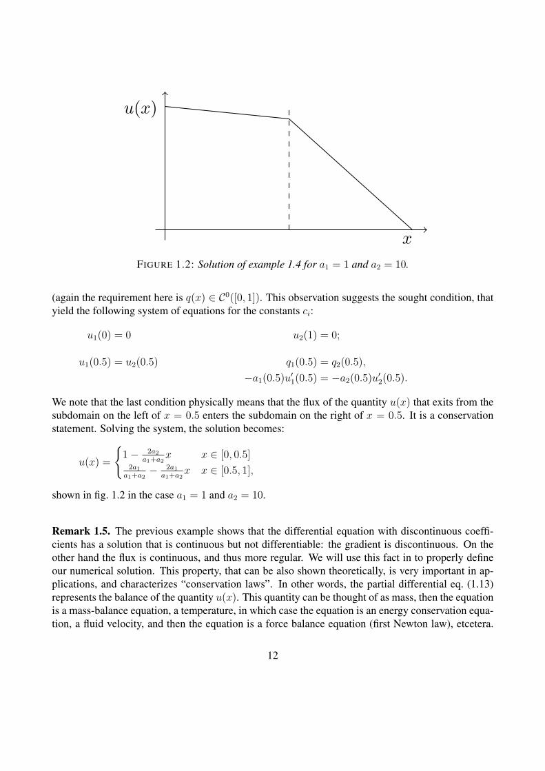
FIGURE 1.2: Solution of example 1.4 for a1 = 1 and a2 = 10.
(again the requirement here is q(x) ∈ C0([0, 1]). This observation suggests the sought condition, thatyield the following system of equations for the constants ci:
u1(0) = 0 u2(1) = 0;
u1(0.5) = u2(0.5) q1(0.5) = q2(0.5),
−a1(0.5)u′1(0.5) = −a2(0.5)u′2(0.5).
We note that the last condition physically means that the flux of the quantity u(x) that exits from thesubdomain on the left of x = 0.5 enters the subdomain on the right of x = 0.5. It is a conservationstatement. Solving the system, the solution becomes:
u(x) =
1− 2a2
a1+a2x x ∈ [0, 0.5]
2a1a1+a2
− 2a1a1+a2
x x ∈ [0.5, 1],
shown in fig. 1.2 in the case a1 = 1 and a2 = 10.
Remark 1.5. The previous example shows that the differential equation with discontinuous coeffi-cients has a solution that is continuous but not differentiable: the gradient is discontinuous. On theother hand the flux is continuous, and thus more regular. We will use this fact in to properly defineour numerical solution. This property, that can be also shown theoretically, is very important in ap-plications, and characterizes “conservation laws”. In other words, the partial differential eq. (1.13)represents the balance of the quantity u(x). This quantity can be thought of as mass, then the equationis a mass-balance equation, a temperature, in which case the equation is an energy conservation equa-tion, a fluid velocity, and then the equation is a force balance equation (first Newton law), etcetera.
12

The determination of the conservation properties of numerical discretization schemes is an active andimportant field of research in the case of highly variable diffusion coefficients.We would like to remark that in the case of jumps in the diffusion coefficient we cannot use theproduct rule to expand the left-hand-side of eq. (1.13). In fact we cannot write the following:
−a(x)u′′(x)− a′(x)u′(x) = 0
because both u′′(x) and a′(x) do not exist for x = 0.5. However, the solution u(x) exists and isintuitively sound, i.e., without any singularity, although it does not possess a second derivative. Hence,the equation must be written exclusively as in eq. (1.13). In general, using the chain rule for derivativeis numerically counterproductive even if the regularity of the mathematical objects allows it.
Example 1.6 (Poisson equation). Find u : [0, 1] 7→ R such that:
−u′′ = f(x) x ∈ [0, 1] (1.14)u(0) = u(1) = 0 (1.15)
with
f(x) =
1 if x = 0.5,
0 otherwise..
This is an elliptic equation. The solution if this problem can be found by means of Green’s functionsand is given by:
u(x) =
14(1− x) if 0 ≤ x ≤ 0.5,
14(x− 1) if 0.5 ≤ x ≤ 1.
(1.16)
This solution is continuous but it has a piecewise constant first derivative with a jump in x = 0.5.Hence the second derivative u′′(x) does not exists in the midpoint. This seems a contradiction asin this case the left-hand-side of eq. (1.14) does not exists for all x ∈ [0, 1]. However, the solutionu(x) given in eq. (1.16) in terms of the integral of the Green’s function is mathematically sound.Thus we need to define a more “forgiving” formulation, whose solution can have discontinuous firstderivatives. This is the role of the so called “weak” formulation to be seen in the next sections.
Example 1.7. Transport equation.Given a vector field of constant velocity λ > 0, find the function u = u(x, t) such that:
ut + λux = 0, (1.17a)u(x, 0) = f(x). (1.17b)
13

-
x
t
x− λt = ξ
ξ
−xλ
6
t = t1
-
bbbbbbb
bbbbbbb
u
xx x+ λt
t = 0
6
FIGURE 1.3: Left panel: characteristic lines for eq. (1.17a) in the (x, t) plane. Right panel: graphof the solution u(x, t) at t = 0 and t = t1 > 0 in the (u, x) plane. The solution is a wave with shapegiven by f(x) (a line in this case) that propagates towards the right with speed λ.
The characteristic curve is a line in the plane (x, t) given by:
x− λt = const = ξ.
Along this line the original eq. (1.17a) becomes:
du
dt=
∂
∂tu(ξ + λt, t) = λux + ut = 0.
Hence, the solution u is constant along a characteristic curve and this constant is determined by theinitial conditions eq. (1.17b):
u(x, t) = f(ξ) = f(x− λt). (1.18)
At a fixed time t1 the solution is given by the rigid translation of the initial condition (f(x)) by aquantity λt1, as shown in fig. 1.3 (right panel).
Example 1.8. Advection (or convection) and diffusion equation (ADE).
14

Find the function u(x, t) : [0, T ]× R 7→ R such that:
∂u
∂t= D
∂u2
∂x2− v∂u
∂c, (1.19a)
u(x, t) = 1 for x = 0, (1.19b)u(x, t) = 0 for x 7→ ∞, (1.19c)u(x, 0) = 0 for t = 0 and x > 0, (1.19d)u(x, 0) = 1 for t = 0 and x = 0. (1.19e)
The solution is given by [3]:
u(x, t) =1
2
[erfc
(x− vt2√Dt
)+ exp
( vxDt
)erfc
(x+ vt
2√Dt
)],
where the function erfc is the complementary error function.
1.2.3 Conservation laws
From the physical point of view, the problems that we are facing are related to the principle of con-servation. For example the equilibrium of an elastic string fixed at the end points and subject toa distributed load is governed by an equation that determines the vertical displacement u(x) of thepoints ox of the string and its tension stresses σ(x), once the load g(x) and the elastic characteristicsof the string E (Young’s modulus) are specified. The problem is written as:
σ(x) = Eu′(x) Hook’s law;
−σ′(x) = g(x) Elastic equilibrium;
u(0) = u(1) = 0 Boundary conditions.
Another interpretation of the same problem can be thought of as u(x) being the temperature of a rodsubjected to a heat source g(x). In this case the symbol k is generally used in place of E to identifythe thermal conductivity of the rod material and q(x) is the heat flux. The model thus is written as:
q(x) = −ku′(x) Fourier’s law; (1.20a)q′(x) = g(x) Energy conservation; (1.20b)u(0) = u(1) = 0 Boundary conditions. (1.20c)
The same equation can be thought as governing the diffusion of a substance dissolved in a fluid. Inthis case we talk about Fick’s law, concentration u(x). diffusion coefficient k, solute mass flux q(x).Yet another interpretation of the same equation is the flow of water in a porous material. We talkthen about Darcy’s law. More in general, we can say that all these equations represent a conservationprinciple. In fact, eq. (1.20a) represents the conservation of momentum deriving from Newton secondlaw (F = ma), while eq. (1.20b) states the conservation of the energy of the system.
15

All these problems are equations written in “divergence form” or in conservative form. For example,consider the advection-diffusion equation (eq. (1.19a)). From the physical point of view, our solutionfunction u represents the density of the conserved quantity. Thus we can introduced the density fluxof this quantity as:
~q = −D∇u+ ~vu,
where the first term on the right-hand-side represents the diffusive flux and the second term representsthe advective flux (the quantity u is transported by the velocity ~v and at the same time is diffused).Equation (1.19a) can then be re-written as:
∂u
∂t+ div ~q = f(x).
The first term represents the variation in time of the mass of this quantity. The second term representsthe variation in space. Integrating the above equation in a subset U ⊂ Ω of the domain we have:∫
U
∂u
∂t+ div ~q dx =
∫U
f(x),
and assuming the boundary of U to be smooth, we can apply the divergence theorem:∫U
∂u
∂tdx+
∫∂U
~q · ν ds =
∫U
f(x).
We recognize the classical mass conservation principle:
rate of change = inflow-outflow
Note that from a purely mathematical point of view, writing the equation in divergence form has noformal advantage with respect to any other alternative formulation. However, this is not true for thenumerical formulation, in which the divergence form is always to be preferred.
1.3 Well posedness and continuous dependence of solutions on the dataThe question of finding a solution to a PDE rests on the definition of solution. We can state that asolution is a function that satisfies the equation and has certain regularity properties 3. However, theanswer to the question what is a solution can be tricky. For a clear account and several interestingexamples see [4]. We report here a few remarks that are useful for the developments and analysis ofnumerical methods.We talk about a “classical” solution of a k-th order PDE to indicate a function that satisfies thePDE and the auxiliary conditions and that is k times differentiable. This is an intuitive requirementso that the derivatives that appear in the expression of the PDE can be formally calculated without
3This last request has to be made to avoid trivial and non interesting solutions.
16

worrying about singularities. However, this notion is often too restrictive, and there may be functionsthat are less regular that indeed satisfy the PDE and the auxiliary conditions. Moreover, by thisstrong regularity requirements, we may restrict the search of solutions only to cases that have enoughregularity of the auxiliary conditions and of the data of the problem (e.g. the coefficients of thePDE). Thus we usually resort to a less restrictive definition of a solution, which is called a “weak”solution. Thus we need to change the formulation of the PDE to accommodate this lower regularityrequirement, maintaining at the same time the physical notion of the process that lead to the PDE.
Remark 1.9. Example 1.4 gives an instance of the application of this concept: the global solution, i.e.,the solution over the entire domain I = [0, 1], is continuous but its derivative is not. Thus a classicalsolution to the problem does not exist, but a “weak” solution can be defined by appropriately relaxingthe continuity conditions of the search space (the space of functions that are candidate solutions).
In any case, it is intuitive to look for solutions that are unique. There is certainly no hope to be able tofind numerically a solution that is not unique. In fact, any computational algorithm in this case wouldnever converge and would oscillate continuously among the several solutions of the problem. Butuniqueness is not sufficient. We also require the notion of “continuous dependence of the solutionform the data of the problem”. In essence, we require that, if for example some coefficients arechanged slightly, then the solution changes slightly. This notion is useful for two important reasons.First, in a computer implementation of any algorithm there is no hope to be able to specify a coefficient(which is a real number) with infinite accuracy. Next, and probably more importantly, uncertaintiesin physical constants or functions are intrinsically present in any model of a physical process. Thisuncertainty results in values of, e.g., boundary conditions or forcing functions that are not knownprecisely. But it is highly desirable that our mathematical model governing the physics be relativelyinsensitive to these uncertainties. This is reflected within the concept of well-posedness that we canmake a little bit more formal by stating the following:
Definition 1.10 (Well posedness). Given a problem governed by a k-th order PDE:
F (x, u, ∂u, . . . , ∂ku,Σ) = 0
where Σ denotes the set of the data defining the problem, we say that this problem is well posed if:
1. the solution u exists;
2. the solution u is unique;
3. the solution u depends continuously on the data, i.e., if one element σ ∈ Σ is perturbed by aquantity δ, the corresponding solution u to the perturbed problem is such that ‖u− u‖ ≤ L ‖δ‖.
Note that this is not a very precise statement, as we need to specify what we mean with the symbol‖·‖. But this definition depends on the functions with which we are dealing, and thus it must beanalyzed and specified for each problem.
17

These three requirements are obvious, especially in the context of numerical solution of a mathemat-ical problem. The first requirement states the incontrovertible fact that we cannot possibly think offinding a numerical approximation of the solution if this does not exist. The second statement assertsthat the solution is unique as a function of the data (for a given set of data). No numerical schemecan approximate simultaneously two different solutions to the same problem, so we can only hope tofind one of them, but in general we get a numerical solution that oscillates between the two and doesnot make sense. If there are more than two solutions the situations is obviously worse. Finally, thelast condition is the most important one. In practical applications we are not so much concerned withthe PDE itself but mainly with its solution, which generally gives the so called “state” of the system.As such, a solution of the PDE is “physically” meaningful if small changes in the data (the parame-ters) of the problem cause small changes to the solution. In other words, a mathematical model of aphysical phenomenon in general will not be useful if small errors in the measured data would lead todrastically different solutions.As an example, consider the PDE of equation eq. (1.1) with the auxiliary conditions eq. (1.2). It isa well posed problem as it satisfies all the three conditions above. However, assume that we are atsteady state, i.e., ∂u/∂t = 0, there are no source/sink, i.e., f = 0, and that only Neumann BCs areimposed, i.e. the only auxiliary condition present in our problem is eq. (1.2c). Then, any constantfunction u(x, t) = C is a solution of the problem, independently of the value of C. Thus the solutionis not unique, and we cannot possibly hope to find it numerically.In practice, the question of whether a PDE problem is well posed can depend also on the auxiliaryconditions that we impose. Generally, if these auxiliary conditions are too many then a solution maynot exist. If they are too few, then the solution may not be unique. And they must be “consistent”with the PDE or the solution may not depend continuously on the data. Thus the question of well-posedness can be difficult to assess.
1.3.1 Ill-conditioning and instability
Two more concepts that are related to well-posedness need to be clearly stated when we move fromthe continuous setting to the discrete (numerical) setting. The first we would like to discuss is “ill-conditioning”. The “condition” of a problem is a property of the mathematical problem (not of thenumerical scheme used to solve it) and can be stated intuitively as follows:
Definition 1.11 (Ill-conditioning). A mathematical problem is said to be ill-conditioned if small per-turbations on the data cause large variations of the solution.
The definition is problem specific, but a simple example related to linear algebra can be illuminating.
Example 1.12. Consider the following 2× 2 system of linear equations:
3x+ 2y = 2 (1.21)2x+ 6y = −8. (1.22)
18
-7 -5 -3 -1 1 3 5
x
-4
-2
0
2
4
y
-6 -4 -2 0 2 4 6
-4
-2
0
2
4
y=-3x/2+1
y=-x/3-4/3
δ
ε∼δ
-2 -1 0 1 2 3 4
x
-6
-4
-2
0
2
4
y
-2 -1 0 1 2 3 4
-6
-4
-2
0
2
4 1 2
ε>>δ
δ
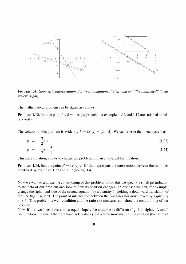
FIGURE 1.4: Geometric interpretation of a “well-conditioned” (left) and an “ill-conditioned” linearsystem (right).
The mathematical problem can be stated as follows:
Problem 1.13. find the pair of real values (x, y) such that examples 1.12 and 1.12 are satisfied simul-taneously.
The solution to this problem is evidently P = (x, y) = (2,−2). We can rewrite the linear system as:
y = −3
2x+ 1 (1.23)
y = −1
3x− 4
3. (1.24)
This reformulation, allows to change the problem into an equivalent formulation:
Problem 1.14. find the point P = (x, y) ∈ R2 that represents the intersection between the two linesidentified by examples 1.12 and 1.12 (see fig. 1.4).
Now we want to analyze the conditioning of this problem. To do this we specify a small perturbationto the data of our problem and look at how its solution changes. In our case we can, for example,change the right hand side of the second equation by a quantity δ, yielding a downward translation ofthe line (fig. 1.4, left). The point of intersection between the two lines has now moved by a quantityε ≈ δ. This problem is well-condition and the ratio ε/δ measures somehow the conditioning of ourproblem.Now, if the two lines have almost equal slopes, the situation is different (fig. 1.4, right). A smallperturbation δ to one if the right hand side values yield a large movement of the solution (the point of
19
intersection), by a quantity ε δ. The conditioning is measured again by the quantity ε/δ which isnow much larger than one. The problem is thus “ill-conditioned”.We note that both problems are actually “well-posed” as they admit a unique solution which is con-tinuously dependent upon the data. But the numerical solution may loose accuracy.
The second concept is called stability. Unlike conditioning, stability is a property of the numericalscheme used to solve a mathematical problem.
Definition 1.15 (Stability). A numerical scheme is stable if errors in initial data remain bounded asthe algorithm progresses.
As an example, consider the following numerical algorithm given by the linear recursion:
u(k) = Au(k−1), k = 1, 2, . . .
where u(k) ∈ Rn, A is a constant n × n matrix, and the recursion is initiated with a given (possiblyarbitrary) initial guess u(0). The representation u(0)
h of the values of u(0) in the computer is not exact,so the actual algorithm involves the numerical approximation u(k)
h :
u(k)h = Au
(k−1)h , k = 1, 2, . . . (1.25)
Stability of the algorithm requires that the errors with which we represent u(0)h are not magnified by
the algorithm process. More formally, we define the error as e(k) = u(k) − u(k)h , k = 1, 2, . . .. From
this last equation we have that u(k) = u(k)h + e(k), and after substitution in eq. (1.25) we obtain the
error propagation equation:
e(k) = Ae(k−1).
Stability of the scheme is achieved if the norm of the error remains bounded as k increases, i.e. (usingcompatible norms):∥∥e(k)
∥∥ ≤ ∥∥Ae(k−1)∥∥ ≤ ‖A‖∥∥e(k−1)
∥∥ ≤ ‖A‖k ∥∥e(0)∥∥
which implies ‖A‖ ≤ 1.Finally we would like to mention the following famous and completely general result known as theLax-Richtmeyer equivalence theorem:
Theorem 1.1 (Lax-Richtmeyer equivalence theorem). A consistent numerical scheme for the solutionof a well posed problem is convergent if and only it is stable.
20

2 Hyperbolic EquationsAn intuitve, although empirical, definition of a hyperbolic equation is as follows. Given x ∈ Rd, thePDE
F (x, u,∇u) = 0
is hyperbolic at the point x if it is possible to transform it into an Ordinary Differential Equa-tion (ODE) with respect to one of the d variables (say xd) as a function of the remaining onesx1, x2, . . . , xd−1.
2.1 Some examplesNotice that in the above statement one of the components of the vector x is take as time (we will dothis often in the sequel). Thus, for example, we can set t := x1 and x := x2, and consider the simpleone-dimensional equation:
ut + ux = 0.
This equation can be transformed into an ODE if we write it along the lines (called “characteristics”):
ξ = x− t.
To see this, we make a simple change of variable x = ξ + t, so that we can write u(x, t) = u(x(t), t)as:
u(x, t) = u(ξ + t, t); x = ξ + t;dx
dt= 1;
dx
dξ= 1,
so that:
d
dtu(ξ + t, t) =
∂u
∂x
dx
dt+∂u
∂t= ut + ux = 0.
From this we see that our original equation is an ODE with respect to time t as a function of space,x (i.e. along the characteristic lines of equation x = ξ + t). Thus, we are mainly interested inlooking at solutions of a Cauchy problem, although we will be looking at the effects of boundaryconditions as well. However, it is intuitive to think that any auxiliary condition on the boundary canbe transformed into an auxiliary condition at t = 0, and vice-versa. Another picture for this statementcan be envisioned by stating that we can revert the sign of the time variable, and go backwards intime, i.e., we can find the solution at an earlier time given the solution at a later time. We will seethat indeed this is the case, contrary to e.g. a parabolic PDE. In other words, a hyperbolic equationgoverns a reversible phenomenon, while a parabolic equation governs a irreversible (or dissipative)phenomenon.
21

t
x
−xλ
ξ
x− λt = ξ
y
xx∗
t = 0
x∗ + λt1
t = t1
FIGURE 2.1: Characteristic line for equation (2.1) in the (x, t) plane (left). Graph of the solutionu(x, t) at t = 0 and t = t1 in the (u, x) plane. A wave of form f(x) (here f(x) = e−a(x−b)2)propagates to the right with speed λ without changing shape.
To study the behavior of a hyperbolic equation, we need to study the geometry of the solution functionin the space of its dependent variables, i.e., z = u(t, x), which represents a surface in Rd+1, if x ∈ Rd.This will help us acquiring an understanding of the type of solutions we may expect from a hyperbolicpartial differential equation. This is what we are trying to do in the next few sections We start thistask with some simple examples.
2.1.1 The transport equation
We look at the simplest PDE that one can devise, i.e., the transport equation. Let us consider thefollowing problem (the same problem already seen in example 1.7):
Problem 2.1. Given a constant velocity vector field q(x)(q1(x), . . . , qd(x)) in a domain Ω ⊂ Rd, finda function u = u(x, t) such that
ut + q · ∇u = 0, in Rd × (0,∞) (2.1a)u(x, 0) = f(x), (2.1b)
Physically, this model represents the motion of particles (solutes, sediments in a fluid) moving withspeed q. It is a conservation law. Indeed:
div(u(t, x)) =∂u
∂t+ div(qu) =
∂u
∂t+ q · ∇u (if div q = 0, i.e., q is a conservative field).
In the one-dimensional case d = 1, the velocity field is one-dimensional λ = q1. In this case thecharacteristic curve is a line in the plane (x, t) given by:
x− λt = const = ξ. (2.2)
22
Along this line the equation takes the form:
du
dt=
∂
∂tu(ξ + λt, t) = λux + ut = 0.
Thus our solution u is constant along the characteristic line. The constant is determined by the initialcondition (2.1b):
u(x, t) = f(ξ) = f(x− λt). (2.3)
We want to see how this general solution can be visualized geometrically. First note that equation (2.3)provides the function u(x, t) in terms of the initial condition (2.1b). The solution at any point (x, t)depends only on the value of f at ξ = x−λt, the intersection of the characteristic line with the x-axis(Figure 2.1, left). We remark that the x-axis is the initial line, i.e., the line at t = 0. We say thatthe “domain of dependence” of u(x, t) on the initial values f(x) is given by the single point ξ. Theinitial values completely determine the solution. They influence the solution only at the points of thecharacteristic line.We can look at the graph of the solution at fixed times. Thus, given the initial condition u(x, 0) =f(x), how does the solution at t = t1, i.e., u(x, t1), look like? It is easy to verify that:
u(x, 0) = u(x+ λt1, t1) = f(x).
This implies that the solution at every fixed time time t is just the rigid translation of the initialcondition along x by the quantity λt. Hence, u(x, t) represents a wave with spatial form given byf(x) that moves to the right (towards increasing x) with speed λ (Figure 2.1, right).
2.1.2 The second-order wave equation
As a classical example of a hyperbolic equation, we consider the second order (one-dimensional)wave equation (1.12). To better understand the geometrical behavior of the solution, we transformthis equation into a system of first order partial differential equations. To this aim, let v = ∂u/∂t andw = ∂u/∂x. Then we have:
∂v
∂t=∂w
∂x∂w
∂t=∂v
∂x.
We can write the previous system in matrix form letting our unknown function u be the vector u =(v, w):
∂
∂t
[vw
]=
[0 11 0
]∂
∂x
[vw
],
23

kt
1t
0t
mt
m−
1t
k−1
tk+
1
xj
x1
x0
xn
xn−1
xj−1
xj+1
t
FIGURE 2.2: Subdivision of the plane (x, t) in a finite difference grid.
or, using an abbreviated notation for the derivative ua = ∂u/∂a:
ut = Aux. (2.4)
We note that matrix A is real, symmetric but not positive definite. It has two distinct real eigenvaluesλ1 = −1 and λ2 = 1 and corresponding normalized eigenvectors e1 = 1√
2[1,−1]T and e2 = 1√
2[1, 1]T .
In all generality, equation (2.4) represents a general system of first order PDEs. We say that such asystem is hyperbolic if matrix A is diagonalizable and has real eigenvalues. This is obviously alwaystrue if A is also symmetric. If the real eigenvalues are distinct then the PDE is “strictly” hyperbolic.
2.1.3 Simple finite difference discretization
We now proceed with the simplest numerical approach for solving (2.1) in the case d = 1, in whichcase we write q = λ, which is assumed positive. Hence, our model problem is:
ut + λux = 0 u(x, 0) = u0(x) (λ > 0)
We use the finite difference method, that is we use various incremental ratios to approximate the timeand space derivatives. To this aim, we subdivide the temporal and spatial intervals uniformly withsubintervals of dimensions ∆t and ∆x, respectively, whereby xj = x0 + j∆x, j = 0, . . . , n and
24

tk = t0 + k∆t, k = 0, . . . ,m and denote by ukh,j = u(xj, tk) the numerical approximation of thesolution at the grid point (j, k) (Figure 2.2). We can approximate the temporal and spatial derivativesusing simple incremental fractions with size ∆x or ∆t or even 2∆x or 2∆t. We obtain the following:
ut(xj, tk) ≈uk+1h,j − ukh,j
∆tut(xj, tk) ≈
uk+1h,j − uk−1
h,j
2∆t
ux(xj, tk) ≈ukh,j+1 − ukh,j
∆xux(xj, tk) ≈
ukh,j − ukh,j−1
∆xux(xj, tk) ≈
ukh,j+1 − ukh,j−1
2∆x
We can then use first forward discretizations of the first derivatives both in space and time to write thefollowing difference equation:
uk+1h,j − ukh,j
∆t= −λ
ukh,j+1 − ukh,j∆x
which can be written by setting µ = λ∆t/∆x as:
uk+1h,j = ukh,j − µλ
(ukh,j+1 − ukh,j
)= (1 + µλ)ukh,j − µλukh,j+1 (2.5)
It is easy to see that this method is consistent, i.e., substitution of the real solution u in place of thenumerical solution uh, yields a residual that goes to zero as ∆t and ∆x tend to zero. This is readilyobtained using the following Taylor series expansions:
u(xj + ∆x, tk) = u(xj, tk) + ux(xj, tk)∆x+ uxx(xj, tk)∆x2
2+O
(∆x3
)u(xj, tk + ∆t) = u(xj, tk) + ut(xj, tk)∆t+ utt(xj, tk)
∆t2
2+O
(∆t3)
and substituting the real solution u(xj, tk) in place of ukh,j into eq. (2.5) we can calculate the residual(local truncation error) as:
τh(xj, tk) =u(xj, tk) + ut(xj, tk)∆t+ utt(xj, tk)∆t2
2+O
(∆t3)
− (1 + µλ)u(xj, tk) + µλ
(u(xj, tk) + ux(xj, tk)∆x+ uxx(xj, tk)
∆x2
2+O
(∆x3
))=utt(xj, tk)
∆t2
2+O
(∆t3)
+ µλ
(uxx(xj, tk)
∆x2
2+O
(∆x3
)), (2.6)
which shows that the local error tends to zero with the discretization size ∆t and ∆x. Since this isa local error (betweeen two mesh nodes and two time steps), the global error is one order less, i.e.,
25

O (∆t+ ∆x). Other schemes can be devised and analyzed. We can write the following:
uk+1h,j =ukh,j − µλ
(ukh,j+1 − ukh,j
)forward Euler - downwind
uk+1h,j =ukh,j − µλ
(ukh,j − ukh,j−1
)forward Euler - upwind
uk+1h,j =ukh,j −
µλ
2
(ukh,j+1 − ukh,j−1
)forward Euler - central
uk+1h,j =uk−1
h,j − µλ(ukh,j+1 − ukh,j−1
)leap-frog
uk+1h,j =
ukh,j+1 + ukh,j−1
2− µλ
2
(ukh,j+1 − ukh,j−1
)Lax-Friedrichs
However, convergence towards the real solution is not guaranteed by consistency alone, as stated bythe Lax-Richtmeyer equivalence theorem (theorem 1.1), but requires that the scheme be stable. Weneed to define stability in the case of our FD approximations, but also we need to properly define con-vergence, although the latter one is a more intuitive concept. We will not dwelve into these issues, atthe heart of numerical analysis, but give only an intuitive and practical explanation of these concepts.
Example 2.2. Solve the transport problem:
ut + ux =0
u(x, 0) =
1− | x | if | x |≤ 1,
0 otherwise.
using the above schemes.
Algorithm 1 Forward-Backward finite difference method for one-dimensional transport equation withconstant velocity. We use periodic boundary conditions and assume the velocity of propagation ispositiv λ > 0. This implies that periodic BC must be implemented for the first node of the FD meshand nothing is imposed on the last node.
1: Set λ > 0; a, b (interval boundaries); ∆x; T (final time); ∆t;2: N = (b− a)/∆x; M = T/∆t; µ = λ∆t/Dx.3: for j = 1, 2, . . . , N do4: uh,j = u0(a+ (j − 1) ∗∆x);5: end for6: for k = 1, . . . ,M do7: uh,1 = (1− λµ)uh,1 + λµuh,N+1
8: for j = 2, . . . , N do9: uh,j = (1− λµ)uh,j + λµuh,j−1
10: end for11: end for
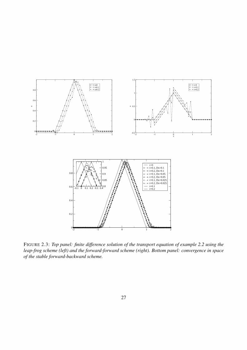
We report in fig. 2.3 (top row) the results obtained at t = 0.1 and t = 0.2 using the leap-frog (leftpanel) and the forward-forward (right panel) schemes. We see immediately that the leap-frog shows
26
-2 -1 0 1 20
0.2
0.4
0.6
0.8
u
t=0t=0.1t=0.2
-2 -1 0 1 2x
-0.5
0
0.5
1
1.5
u
t=0t=0.1t=0.2
-2 -1 0 1 20
0.2
0.4
0.6
0.8
t=0t=0.1, Dx=0.1t=0.2, Dx=0.1t=0.1, Dx=0.05t=0.2, Dx=0.05t=0.1, Dx=0.025t=0.2, Dx=0.025t=0.1t=0.2
0.8
0.85
0.9
0.95
1
-0.1 0 0.1 0.2 0.3 0.4
t=0t=0.1, Dx=0.1t=0.2, Dx=0.1t=0.1, Dx=0.05t=0.2, Dx=0.05t=0.1, Dx=0.025t=0.2, Dx=0.025t=0.1t=0.2
FIGURE 2.3: Top panel: finite difference solution of the transport equation of example 2.2 using theleap-frog scheme (left) and the forward-forward scheme (right). Bottom panel: convergence in spaceof the stable forward-backward scheme.
27

some small oscillations at the left foot of the wave, but the forward-forward shows large oscillationsthat prevent any visually correct representation of the solution. The bottom row reports the behaviorof the forward-backward scheme, implemented following algorithm example 2.2. The results areobtained at two successive refinements of the spatial grid (halving each time the value of ∆x) andshow experimentally the convergence of the numerical solution towards the real solution, representedby the translation of the initial conditions by a quantity λt.
We would like to explain the behavior of the three schemes seen in the previous example. Hence weneed to test the stability of the schemes. To this aim we introduce the shift operator Eh defined as
Ehg(x) = g(x+ ∆x),
we can formally write:
uk+1h,j = (1 + µλ− µλEh)ukh,j = Thu
kh,j
where Th is the so called “transfer operator” (spatial transfer). To ascertain stability we need to lookat the error and its norm, defined as:
εkh,j = ukh,j − u(xj, tk);∥∥εkh,·∥∥ =
(∆x
∞∑j=−∞
| εkh,j |p) 1
p
which are a discrete approximation of the real error εh(x, t) and its Lp norm. Because of linearity, wecan write:
uk+1h,j = Thu
kh,j = Th
(εkh,j + u(xj, tk)
),
from which we have:
εk+1h,j =uk+1
h,j − u(xj, tk+1)
=Thukh,j − u(xj, tk+1)
=Th(εkh,j + u(xj, tk)
)− u(xj, tk+1)
=Th(εkh,j + u(xj, tk)
)− Thu(xj, tk) + Thu(xj, tk)− u(xj, tk+1)
=Th(εkh,j + u(xj, tk)
)− Thu(xj, tk) +
τh(xj, tk+1)
∆t.
Taking norms and using the triangular inequality, we have now:∥∥εk+1h,j
∥∥ ≤∥∥Th (εkh,j + u(xj, tk))− Thu(xj, tk)
∥∥+‖τh(xj, tk+1)‖
∆t
≤CT∥∥εkh,j∥∥+
‖τh(xj, tk+1)‖∆t
28

where CT is the norm of the operator Th. If CT < 1, i.e., Th is contractive, looking at the expressionfor τh(x, t), we see that the scheme converges as ∆t and ∆x tend to zero if sup | utt | and sup | uxx |are bounded.A better look at the error can be derived as follows. By induction on k, the scheme can be written as:
ukh,j = (1 + µλ− µλEh)ku0h,j.
and thus, by linearity and using consistency, we have that:
εkh,j = (1 + µλ− µλEh)kε0h,j
Using the binomial theorem 4:
ukh,j = (1 + µλ− µλEh)ku0h,j =
k∑r=0
(k
r
)(1 + µλ)r(−µλEh)k−rf(x)
=k∑r=0
(k
r
)(1 + µλ)r(−µλ)k−rfh(x+ (k − r)∆x),
where fh(x + j∆x) is the numerical representation of the initial data function f(x) at x = xj . Wedefine the domain of dependence for this difference equation for ukh,j as the set of points x, x +∆x, . . . , x + k∆x, i.e., the set of grid points in the x-axis that lie between x and x + k∆x. Aswe have seen, the domain of dependence for the original equation is given by the single point ξ =x − λt = x − λkµ∆x: the domain of dependence of the difference equation does not contain in thedomain of dependence of the differential equation. The initial value fh(ξ) is never used in forming thenumerical solution. Thus, it is intuitive that the scheme will not converge to the correct solution. Infact, this scheme fails the “Courant-Friedrichs-Lewy” (CFL) condition, which states that the domainof dependence of the numerical scheme must contain the domain of dependence of the PDE. Thescheme is also not stable, as can be seen easily if we assume that f(x) is calculated with an errordenoted by ε. Then, considering that for even k − r the negative sign cancels and the correspondingterm adds, the error at the k-th step will be approximately:
k∑r=0
(k
r
)(1 + µλ)r(−µλ)k−rε ≈ (1 + 2µλ)kε,
which, being µλ > 0, explodes exponentially with k.If now we use the forward discretization in time and the backward discretization in space, we obtainthe scheme:
uk+1h,j = ukh,j − µλ (ukh,j − ukh,j−1) = (1− µλ+ µλE−1
h )ukh,j, (2.7)
4
(a+ b)n =
n∑j=0
(n
j
)ajbn−j
29

t
x
x− λt = ξ
u1h,3 = u0h,3 + µλ(u0h,3 − u0h,2)
x1 x2 x3 x4 x5 x6
t1
t2
t3
(x3, t1)
t
x
x− λt = ξ
u1h,3 = u0h,3 + µλ(u0h,4 − u0h,3)
x1 x2 x3 x4 x5 x6
t1
t2
t3
(x3, t1)
FIGURE 2.4: Downwind (left) vs. upwind (right) FD in the t− x plane.
u
@@ @@ @@ @@@@
6
-
-
uk1 = 1 — BC u0i = 0 — IC
u12 = (1− λ∆t
∆x)u0
2 + λ∆t∆xu0
1
. . . . . .
uk+1j = (1− λ∆t
∆x)ukj + λ∆t
∆xukj−1
x1 x2 x3 x4 x5
λ∆t
x
FIGURE 2.5: Upwind FD in the u− x plane. Crosses denote grid points in space. We can easily seethat for λ∆t
∆x= 1, i.e., CFL = 1, the upwind FD scheme returns the exact solution.
30

where E−1h uh,j = uh,j−1. Written in terms of the initial data, we have the equivalent difference
equation:
ukh,j = (1− µλ+ µλE−1h )ku0
h,j =k∑r=0
(k
r
)(1− µλ)r(µλE−1
h )k−rfh(xj)
=k∑r=0
(k
r
)(1− µλ)r(µλ)k−rfh(x− (k − r)∆x).
Now the domain of dependence of the scheme is the set of points
x, x−∆x, x− k∆x = x− t
µ.
At convergence (∆x,∆t 7→ 0, keeping µ = ∆x/∆t constant) this set tends to the interval [x−t/µ, x].Hence the Courant-Friedrichs-Lewy condition is satisfied if the this interval contains the point ξ =x− λt, i.e. if µ satisfies the stability criterion, or CFL condition (Figure 2.4):
µλ =∆tλ
∆x≤ 1.
The stability of the scheme is proved as before because:k∑r=0
(k
r
)(1− µλ)k(µλ)k−rε = ((1− µλ) + µλ)kε = ε.
It can be shown that the backward (or “upwind”) scheme converges if µλ ≤ 1. In other words, wewant to see that whenever ∆x 7→ 0, j 7→ ∞ and ∆t 7→ 0, k 7→ ∞ in such a way that x = j∆xand t = k∆t, then | u(x, t) − ukh,j |7→ 0. To obtain this, we note that expanding f around the pointξ = x− ct:| u(x, t+ ∆t)− (1− µλ)u(x, t)− µλ u(x−∆x, t) | =
| f(x− λt− λ∆t)− (1− µλ)f(x− λt)− µλ f(x− λt−∆x) |
≤ 1
2(µ2λ2 + µλ) sup
x| f ′′ | ∆x2 ≤ C∆x2,
Indicating with w = u− uh the error function, we have:
| w(x, t+ ∆t)− (1− µλ)w(x, t)− µλ w(x−∆x, t) |≤ C∆x2.
Taking the supx and using the triangle inequality, we can write:
supx| w(x, t+ ∆t) |≤ sup
x| w(x, t) | +C∆x2,
or equivalently, assuming that w(x, 0) = u(x, 0)− u0h,j = f(x)− fh(x) = 0:
| u(x, t)− ukh,j |≤ supx| w(x, k∆t) |≤ sup
x| w(x, 0) | +kC∆x2 =
Ct∆xµ
,
from which convergence is proved since t is fixed and µ = const.
31

2.2 The method of characteristicsA Lagrangian point of view We assume that a certain quantity (energy, density, etc.) is transportedin a velocity field λ(x, t). If we look at the trajectory of every particle, we are using what is called theLagrangian approach, i.e., we try to infer the solution to the problem by measuring data in a referenceframe that moves with λ. If on the other hand we stand at a point x and measure the velocity and itstransported quantity, than we are using the Eulerian approach, i.e., we infer the solution by measuringdata at a fixed set of points. This is what we have done in the previous section.For every initial point x0 ∈ Rd, the trajectory starting from x0 is given by:
dx
dt= q(x, t)
x(0) = x0.
The solution to this ODE is given by x = γx0(t), i.e. a curve written in parametric form γ : Rd 7→ R.If the quantity (call it u(x, t)) transported with the field q does not change in time, its total derivativeis zero:
Dtu =du
dt(γx0(t), t) =
∂u
∂t+ q · ∇u = 0,
which in R1 is written as:
Dtu =du
dt(γx0(t), t) = ut + λux = 0,
i.e., the advection equation we have studied in the previous section.Let us now fix an initial condition. In other words, we want to solve the following transport problem:
ut + λux = 0,
u(x, 0) = f(x).
To find the solution of this problem, we want to find the parameterized curve x = γx0(t) for everyx0 ∈ R such that:
dx
dt= λ(x, t),
x(0) = x0.
For the transported quantity, since Dtu = 0, we have:
u(x, t)x0 = f(x0)
x0 = γ−1x0
(t)
u(x, t) = f(γ−1x0
(t))
32
In other words, the solution u is given by the function f (the initial data) along the characteristic curveγ. The task is thus to find the characteristic curves, along which the signal is propagated “withoutchanging shape”. This last sentence is in quotes as it is true only for linear advection and with nosource term, as we will see in the following examples.
Example 2.3. Find the solution to the problem:
ut + ux = 0, (2.8a)u(x, 0) = sin(x). (2.8b)
In this case, λ = 1, and the ODE determining the trajectories for (2.8) is:
dx
dt= 1,
x(0) = x0,
which has solution given by x = t+ x0, so that:
x0 = x− t,u(x, t) = sin(x− t).
Example 2.4. Find the solution to the problem:
ut + ux = u, (2.9a)u(x, 0) = f(x). (2.9b)
In this case, λ = 1, but the equation is not homogeneous. The ODE for the trajectories of (2.9) is thesame, but now the transported quantity is not conserved any longer as it undergoes a transformationdirectly proportional to u, i.e.:
Dtu = u.
This equation has a general solution given by u(x0, t) = Cet. The complete solution is then given by:
x0 = x− t,u(x, t) = f(x− t)et.
Quasilinear equations Consider the general first order quasilinear equation of the form:
a(x, y, u)ux + b(x, y, u)uy = c(x, y, u), (2.10)
where we may think of the variable x as space and y as time. The solution function is a surfacein the (xyz) space, z = u(x, y), called an “integral surface”. The functions a(x, y, u), b(x, y, u)
33

and c(x, y, u) define a vector field in the (xyz) space, and identify the field of local “characteristicdirections” with direction numbers (a, b, c). The vector normal to the surface z = u(x, t) at each pointis given by (ux, uy,−1). Thus, equation (2.10) details the condition by which the integral surface isat each point tangent to the characteristic direction. We can associate to this surface the family of“characteristic curves” defined so that they are tangent to the direction field at each point. Along acharacteristic curve given in parametric form as (x, y, z) = Γ(σ) = (f(σ), g(σ), h(σ)), the tangentcondition can be written as:
dx
dσ= a(x, y, z),
dy
dσ= b(x, y, z),
dz
dσ= c(x, y, z).
The solution of this system of ODEs is formed by a 3-parameter family of curves (x(σ), y(σ), z(σ))(the parameters corresponding to the constants that arise from solving each of the three ODEs above).This gives rise to a 2-parameter family of characteristic curves, since multiplying the functions a, b, cby a constant is equivalent to scaling the parameter σ so that the equation and its solution are scaledbut not the characteristic curves. It can be shown that there exist a characteristic curve that passesthrough every point of an integral surface, and vice-versa. The integral surface is then the union ofcharacteristic curves. If two integral surfaces intersect at a point P , then they intersect along an entirecharacteristic curve passing through P .As a consequence, a unique solution is defined by choosing one single member of the family ofcharacteristic curves. Let Γ be represented in parametric form by the equations:
x = f(σ), y = g(σ), z = h(σ).
Then the solution u(x, y) in Γ must satisfy the relationship:
h(σ) = u(f(σ), g(σ)). (2.11)
We look only for “local” solutions, i.e., solutions arising for σ in a neighborhood of a point σ0, orequivalently x0 = f(σ0) and y0 = g(σ0). Then varying σ0 we can find other solutions. It can beshown that an integral surface is the union of all these solutions.This gives rise to the Initial Value problem:Find u(x, y) such that:
a(x, y, u)ux + b(x, y, u)uy = c(x, y, u),
and such that
u(x, 0) = h(x).
Remark 2.5. This yields the form of the equation that we have seen in the previous sections. Ofteny coincides with time and thus y ≥ 0, so that the IVP specifies initial data for y = 0. Thus, the
34

initial-value problem is the special Cauchy problem where we have specified the characteristic curveΓ in parametric form as:
Γ :
x = σ,y = 0,z = h(σ).
This shows that in this IVP we look for that integral surface that intersects with the xz-plane (y = 0).
Going back to the general case, given σ we look for the curve Γ that passes through point Pσ =(xσ, yσ, zσ) = (f(σ), g(σ), h(σ)). Looking for “local” solutions, we let σ vary in a neighborhood ofσ, and we form that function (solution) given by the set of points P = (x, y, z), obtained by varyingτ in a neighborhood of P (i.e., centered in σ), that have coordinates:
x = X(σ, τ), y = Y (σ, τ), z = Z(σ, τ), (2.12)
so that they reduce to (f(σ), g(σ), h(σ)) for τ = 0. Thus for every σ we have the following systemof ODEs:
Xτ = a(X, Y, Z), Yτ = b(X, Y, Z), Zτ = c(X, Y, Z)
with corresponding initial conditions:
X(σ, 0) = f(σ), Y (σ, 0) = g(σ), Z(σ, 0) = h(σ).
Now, we can solve for (σ, τ) from the first two equations of (2.12) to get σ = S(x, y) and τ = T (x, y).Substituting in the third equation of (2.12), we have and explicit representation of the solution surfacez = u(x, y):
z = u(x, y) = Z(S(x, y), T (x, y)),
and correspondingly we can find the functions:
x = X(S(x, y), T (x, y)), y = Y (S(x, y), T (x, y)),
satisfying the initial conditions σ0 = S(x0, y0) and τ0 = 0 = T (x0, y0), and thus completing theprocedure of finding the solution to our problem. However, this can be done provided the determinantof the Jacobian matrix does not vanish:
det (J) =
∣∣∣∣ Xσ(σ0, 0) Yσ(σ0, 0)Xτ (σ0, 0) Yτ (σ0, 0)
∣∣∣∣ =
∣∣∣∣ f ′(σ0) g′(σ0)a(x0, y0, z0) b(x0, y0, z0)
∣∣∣∣ 6= 0
Now using (2.11) and the expression of our quasi-linear PDE (2.10) for σ = σ0, x = f(σ0) andy = g(σ0) we can calculate the following relationships:
f ′b = g′a, h′ = f ′ux + g′uy, c = aux + buy,
35
from which we obtain:
bh′ = cg′ and ah′ = cf ′.
In practice this shows that det (J) = 0 implies that f ′, h′, and g′ are proportional to a, b and c, i.e., thevector field (f ′, g′, h′) is parallel to the vector field (a, b, c) and thus defines again the characteristicspassing through σ0, showing that this procedure is well defined.
Example 2.6. Find the solution to the problem:
uy + cux = 0, (2.13a)u(x, 0) = f(x). (2.13b)
In this case, λ = c, the equation is the same as (2.1). The characteristic ODEs corresponding to (2.13)becomes the following system:
dx
dτ= c,
dy
dτ= 1,
dz
dτ= 0,
or:
dx
dτ= c, Dyu = 0.
The integral surface has the parametric representation:
x = X(σ, τ) = σ + cτ, y = Y (σ, τ) = τ, z = Z(σ, τ) = f(σ).
Eliminating σ and τ we obtain the solution:
z = u(x, y) = f(x− cy).
Example 2.7. Find the solution to the problem:
uy + uux = 0, (2.14a)u(x, 0) = f(x). (2.14b)
In this case, λ = u, but the equation is now non linear (quasi linear). The system of characteristicODEs corresponding to (2.14) is:
dx
dτ= u,
dy
dτ= 1,
dz
dτ= 0,
or:
dx
dτ= u, Dτu = 0,
36

to which we need to add the initial data (2.13b). The solution of this system leads to the parametricform:
x = σ + uτ, y = τ, z = f(σ).
The solution u = u(x, τ) = u(x, y) is given then by:
u(x, y) = f(x− uy).
The projection of the characteristic curve in the plane xy is given by the line (named Cσ):
x = σ + f(σ)y.
Along Cσ the solution assumes the form u = f(σ). Note that strictly speaking a characteristiccurve lies in an integral surface in the space xyz. However, its projection is often called also acharacteristic curve. We will use this nomenclature, as there is no worry of confusion given thedifferent dimensionality of the two curves, but we will name Γ and Cσ the characteristic curve in xyzand its projection onto xy, respectively. The curve Cσ represents the trajectory of a particle initially(at time y = 0) located at x = σ. Depending on the value of f(σ), the characteristic curves mayhave different slopes. Thus, in general, two characteristic curves intersect at a point unless f(σ) is anondecreasing function of σ. Given two characteristics Cσ1 and Cσ2 expressed by:
Cσ1 : x = σ1 + f(σ1)y
Cσ2 : x = σ2 + f(σ2)y
they intersect at the point (x, y) given by:
y = − σ2 − σ1
f(σ2)− f(σ1), x = σ + f(σ)y.
If σ1 6= σ2 and f(σ1) 6= f(σ2), u at the point (x, y) must take distinct values given by f(σ1) andf(σ2), and thus the function u is not one-to-one. Looking at the first derivative of u, we can write:
u(x, y) = f(x− uy); ux = f ′(σ)dσ
dx=
∂
∂x(x− u(x, y)y) = 1− yux,
from which we obtain:
ux =f ′(σ)
1 + yf ′(σ).
Hence, if f ′(σ) < 0, ux becomes infinite at time:
y =−1
f ′(σ). (2.15)
The smallest time at which this occurs corresponds to the value σ = σ0 at which f ′ has a minimum.Thus the solution to equation (2.14) is unique only until the finite time T = −1/f ′(σ0).
37

-3 -2 -1 0 1 2 3x
0
1
2
3
4
5
t
T
FIGURE 2.6: Characteristic lines for the equation in Example 2.8.
Example 2.8. We now look at this problem from a physical (geometrical) point of view, i.e., we lookat how the solution looks like qualitatively, and why the loss of uniqueness occurs. We will look atthe following particular case where f(x) = 1/(1 + x2) (here we will use the more common variablename t for y). The problem is then:Find the solution u(x, t) such that
ut + uux = 0, (2.16a)
u(x, 0) =1
1 + x2. (2.16b)
This is called the “inviscid Burgers” equation. As seen before, since the directional derivative vanishesalong the direction of the vector (1, u), the solution u must be constant along the characteristic linesCσ in the plane t, x given by:
Cσ : (t, x+ u(x, 0)t) = (t, x+t
1 + x2).
There the solution is given implicitly by:
u(x+t
1 + x2, t) =
1
1 + x2. (2.17)
38
-2 -1 0 1 2 3x
0.2
0.4
0.6
0.8
1
1.2
u
u(0) u(T1) u(T2)
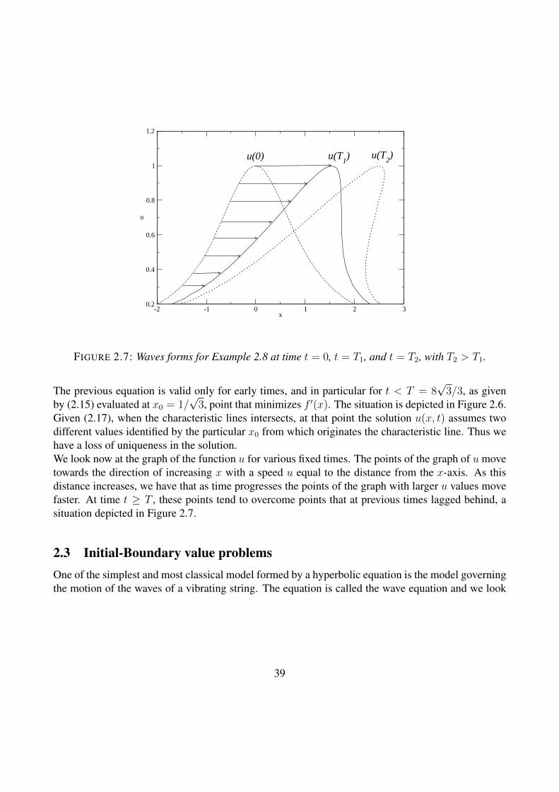
FIGURE 2.7: Waves forms for Example 2.8 at time t = 0, t = T1, and t = T2, with T2 > T1.
The previous equation is valid only for early times, and in particular for t < T = 8√
3/3, as givenby (2.15) evaluated at x0 = 1/
√3, point that minimizes f ′(x). The situation is depicted in Figure 2.6.
Given (2.17), when the characteristic lines intersects, at that point the solution u(x, t) assumes twodifferent values identified by the particular x0 from which originates the characteristic line. Thus wehave a loss of uniqueness in the solution.We look now at the graph of the function u for various fixed times. The points of the graph of u movetowards the direction of increasing x with a speed u equal to the distance from the x-axis. As thisdistance increases, we have that as time progresses the points of the graph with larger u values movefaster. At time t ≥ T , these points tend to overcome points that at previous times lagged behind, asituation depicted in Figure 2.7.
2.3 Initial-Boundary value problemsOne of the simplest and most classical model formed by a hyperbolic equation is the model governingthe motion of the waves of a vibrating string. The equation is called the wave equation and we look
39
(x,t)
t
x
x−vt=ξ ηx+vt=
x−vt x+vt
t
x
x−vt=ξ ηx+vt=
x−vt x+vt
(x,t)
ξ
A
B
C
D
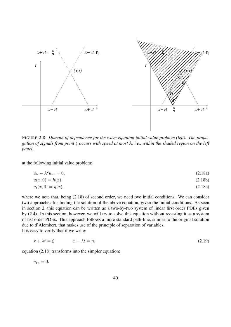
FIGURE 2.8: Domain of dependence for the wave equation initial value problem (left). The propa-gation of signals from point ξ occurs with speed at most λ, i.e., within the shaded region on the leftpanel.
at the following initial value problem:
utt − λ2uxx = 0, (2.18a)u(x, 0) = h(x), (2.18b)ut(x, 0) = g(x), (2.18c)
where we note that, being (2.18) of second order, we need two initial conditions. We can considertwo approaches for finding the solution of the above equation, given the initial conditions. As seenin section 2, this equation can be written as a two-by-two system of linear first order PDEs givenby (2.4). In this section, however, we will try to solve this equation without recasting it as a systemof fist order PDEs. This approach follows a more standard path-line, similar to the original solutiondue to d’Alembert, that makes use of the principle of separation of variables.It is easy to verify that if we write:
x+ λt = ξ x− λt = η, (2.19)
equation (2.18) transforms into the simpler equation:
uξη = 0.
40
This equation states that uξ is independent of η, i.e., it is a function of ξ: uξ = f(ξ). After integration,we have that
u(ξ, η) =
∫f(ζ)dζ +G(η) = F (ξ) +G(η),
i.e., u(ξ, η) is the sum of two functions of ξ and η, respectively. Using (2.19), we have the solution inthe original variables:
u(x, t) = F (x+ λt) +G(x− λt). (2.20)
The form of this solution shows a superposition of two waves, solutions of vt − λvx = 0 and wt +λwx = 0, respectively. This corresponds to the fact that the differential operator can be factored intothe product of two operators:
L =
(∂2
∂t2− λ ∂
2
∂x2
)=
(∂
∂t− λ ∂
∂x
)(∂
∂t+ λ
∂
∂x
).
If we impose the initial conditions (2.18b) and (2.18c) we obtain:
u(x, 0) = F (x) +G(x) = h(x) (2.21)ut(x, 0) = λF ′(x)− λG′(x) = g(x). (2.22)
Differentiating the first equation and solving the ensuing linear system for F (x) and G(x) we obtain:
F ′(x) =λh′(x) + g(x)
2λG′(x) =
λh′(x)− g(x)
2λ
yielding after integration:
F (x) =h(x)
2+
1
2λ
∫ x
0
g(ζ)dζ + C1
G(x) =h(x)
2− 1
2λ
∫ x
0
g(ζ)dζ + C2
From (2.21), we have immediately C1 + C2 = 0, from which we obtain:
u(x, t) = F (x+ cλt) +G(x− λt) =1
2(h(x+ λt) + h(x− λt)) +
1
2λ
∫ x+λt
x−λtg(τ)dτ. (2.23)
The above general solution to the wave equation is determined uniquely by the values of h and g fort = 0, that is from the initial data (2.18b) and (2.18c). The fact that we have x ± λt as argument ofthe initial functions tells us that the domain of dependence of u(x, t) is the triangular region shownin Figure 2.8. In other words, given a point (x, t), the solution u at that point depends only upon thevalues of u in the domain of dependence.
41
t
x
λ < 0t
x
λ > 0
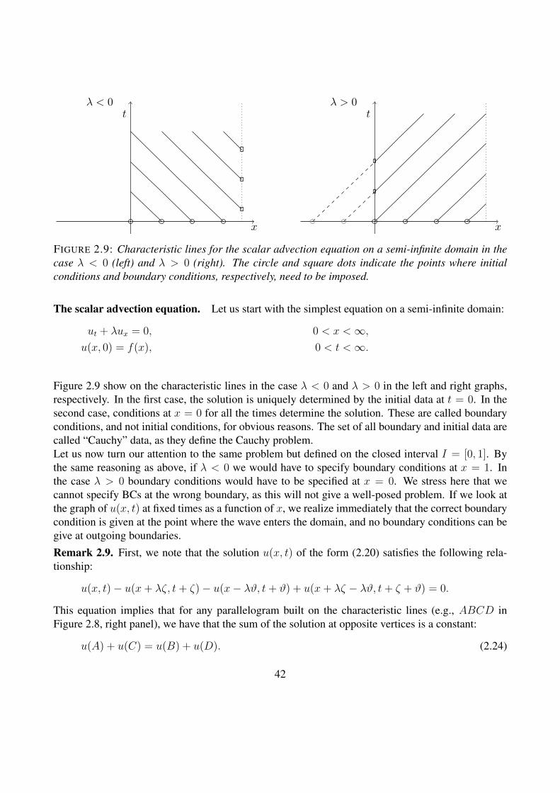
FIGURE 2.9: Characteristic lines for the scalar advection equation on a semi-infinite domain in thecase λ < 0 (left) and λ > 0 (right). The circle and square dots indicate the points where initialconditions and boundary conditions, respectively, need to be imposed.
The scalar advection equation. Let us start with the simplest equation on a semi-infinite domain:
ut + λux = 0, 0 < x <∞,u(x, 0) = f(x), 0 < t <∞.
Figure 2.9 show on the characteristic lines in the case λ < 0 and λ > 0 in the left and right graphs,respectively. In the first case, the solution is uniquely determined by the initial data at t = 0. In thesecond case, conditions at x = 0 for all the times determine the solution. These are called boundaryconditions, and not initial conditions, for obvious reasons. The set of all boundary and initial data arecalled “Cauchy” data, as they define the Cauchy problem.Let us now turn our attention to the same problem but defined on the closed interval I = [0, 1]. Bythe same reasoning as above, if λ < 0 we would have to specify boundary conditions at x = 1. Inthe case λ > 0 boundary conditions would have to be specified at x = 0. We stress here that wecannot specify BCs at the wrong boundary, as this will not give a well-posed problem. If we look atthe graph of u(x, t) at fixed times as a function of x, we realize immediately that the correct boundarycondition is given at the point where the wave enters the domain, and no boundary conditions can begive at outgoing boundaries.
Remark 2.9. First, we note that the solution u(x, t) of the form (2.20) satisfies the following rela-tionship:
u(x, t)− u(x+ λζ, t+ ζ)− u(x− λϑ, t+ ϑ) + u(x+ λζ − λϑ, t+ ζ + ϑ) = 0.
This equation implies that for any parallelogram built on the characteristic lines (e.g., ABCD inFigure 2.8, right panel), we have that the sum of the solution at opposite vertices is a constant:
u(A) + u(C) = u(B) + u(D). (2.24)
42

We will be using consistently this observation in the following paragraphs to obtain trajectories (setof characteristic lines) of the wave equations in a compact domain.
The wave equation. We want to look now at an Initial-Boundary Value problem for the wave equa-tion. In this case, our equation is specified in a compact domain Ω ∈ Rd, identified in our case byan interval. We can think of Ω = I = [0, 1]. In this case, the solution of our wave equation must berestricted within this interval, and we have to specify additional conditions besides the initial ones,called boundary conditions. However, as we will see, we cannot specify boundary conditions at will.We can state our initial-boundary value problem as:
Problem 2.10. Find u(x, t) such that:
utt − λ2uxx = 0,
u(x, 0) = h(x); ut(x, 0) = g(x),
u(0, t) = α(t); u(1, t) = β(t).
This problem corresponds to restricting all the characteristic lines seen above to the interval [0, 1].However, it is intuitive that if we do this we need to specify certain conditions at x = 0 and x = 1 forall the times. These boundary conditions cannot be arbitrary. For example, at x = 0 we cannot specifyconditions along the characteristic line x+ λt, and vice-versa, at x = 1 we cannot specify conditionsalong the characteristic line x−λt. Moreover, continuity of the solution and continuous dependence ofthe solution to the initial data (i.e., well-posedness) require that we specify these BCs imposing somecompatibility conditions. To see this we work out the solution to our IBV problem 2.10 constructingthe characteristic lines and using Remark 2.9 in the ensuing regions.In the plane x − t the characteristic lines and the domain of dependence can be described as inFigure 2.10. Looking separately at the solution in the different regions, we see that in region I thesolution is determined by the initial data at t = 0, and its expression is given by (2.23). In a point ofregion II, say point A = (x, t), the solution can be evaluated by (2.24) by noting that in B the solutionis given by the left boundary condition, and in C and D by the initial condition. We note that we needto construct the parallelogram using the characteristic lines. Following this method we can determinethe solution at every point of the domain.If the initial data h(x) and g(x) together with the boundary conditions α(t) and β(t) are arbitrarily, thesolution may not be smooth and can have jumps across the characteristic lines. If we want a smooth(C2) solution we need to require that:
α(0) = h(0); α′(0) = g(0); α′′(0) = λ2h′′(0);
β(0) = h(1); β′(0) = g′(1); β′′(0) = λ2h′′(1).(2.25)
Looking at Figure 2.10 it is intuitive that the solution along the characteristic lines x − λt = C isdetermined either by the initial data or by the boundary condition on the left. The boundary condition
43
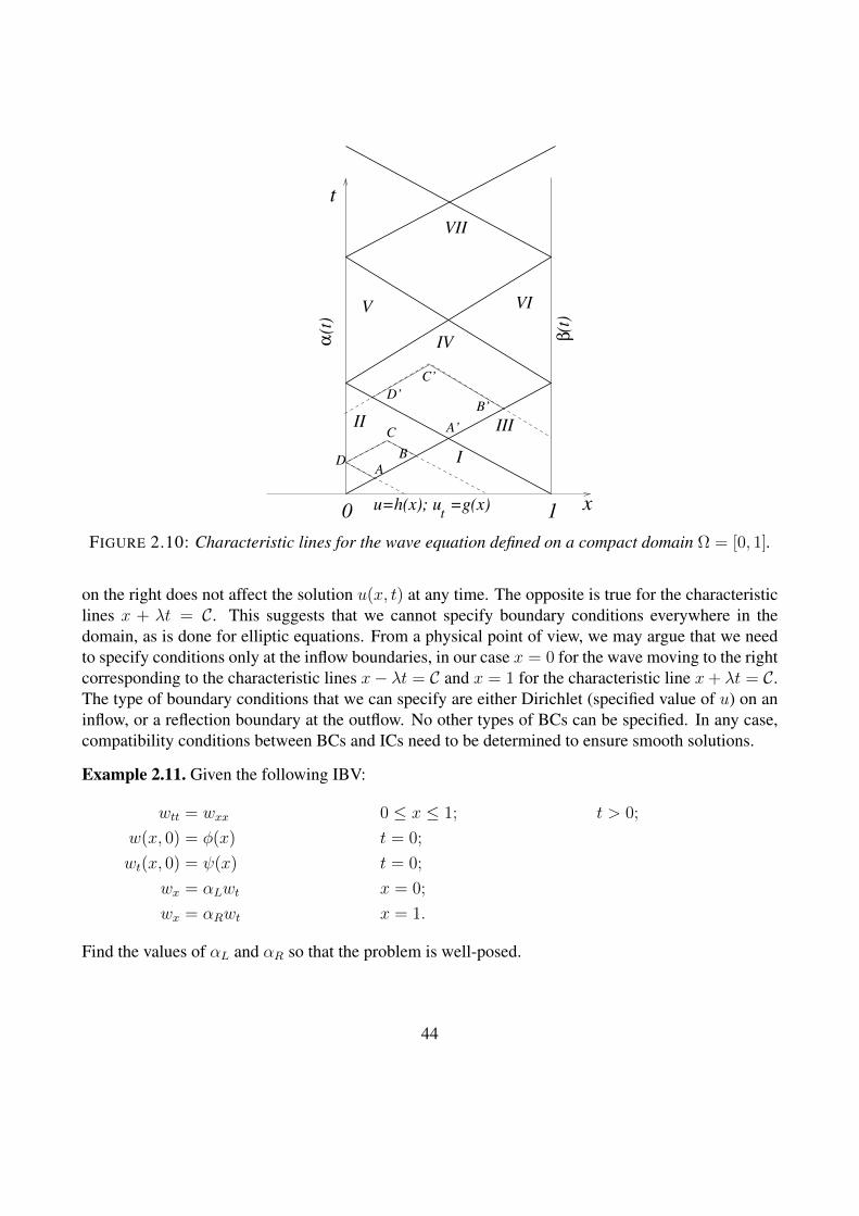
t
(t)
α(t
)
β
x
t
0 1
A
B
C
D
A’
B’
C’
D’
I
II III
IV
V VI
VII
u=h(x); u =g(x)
FIGURE 2.10: Characteristic lines for the wave equation defined on a compact domain Ω = [0, 1].
on the right does not affect the solution u(x, t) at any time. The opposite is true for the characteristiclines x + λt = C. This suggests that we cannot specify boundary conditions everywhere in thedomain, as is done for elliptic equations. From a physical point of view, we may argue that we needto specify conditions only at the inflow boundaries, in our case x = 0 for the wave moving to the rightcorresponding to the characteristic lines x− λt = C and x = 1 for the characteristic line x+ λt = C.The type of boundary conditions that we can specify are either Dirichlet (specified value of u) on aninflow, or a reflection boundary at the outflow. No other types of BCs can be specified. In any case,compatibility conditions between BCs and ICs need to be determined to ensure smooth solutions.
Example 2.11. Given the following IBV:
wtt = wxx 0 ≤ x ≤ 1; t > 0;
w(x, 0) = φ(x) t = 0;
wt(x, 0) = ψ(x) t = 0;
wx = αLwt x = 0;
wx = αRwt x = 1.
Find the values of αL and αR so that the problem is well-posed.
44
Rewrite the wave equation as a system of first-order equations:
ut = Aux; u =
[wtwx
]; A =
[0 11 0
]Matrix A can be diagonalized as:
Λ = UAUT ; Λ =
[−1 00 1
]; U =
1√2
[1 1−1 1
]; UUT = I.
Let v = [vI , vII ]T = Uu. Then the system above transforms into:
vt = Λvx, or[vI
vII
]t
=
[−1 00 1
] [vI
vII
]x
Thus, the original wave equation has been transformed into a system of two separate advection equa-tions. Looking at Example 2.3, we see that vI is a wave propagating with celerity λ = −λ1 = 1while vII has λ = −λ2 = −1 and the characteristic directions are the eigenvectors r1 = (−1, 1)T andr2 = (1, 1)T . Thus we recover the solution developed in Section 2.10.Since we have a wave traveling from left to right and a wave traveling from right to left we needa boundary condition on the left and on the right boundaries, respectively. Intuitively, these BCswill relate vI with vII through the proper well-posed boundary conditions, at x = 0 and x = 1,respectively. To see this, we note that:
v = Ur; r = UTv.
From this we easily obtain:[vI
vII
]=
1√2
[1 1−1 1
] [wtwx
]vI = 1√
2(wt + wx)
vII = 1√2(−wt + wx)
and [wtwx
]=
1√2
[1 −11 1
] [vI
vII
]wt = 1√
2(vI − vII)
wx = 1√2(vI + vII)
At x = 0 the BC prescribes that wx = αLwt, yielding:
vI + vII = αL(vI − vII), or vI =αL + 1
αL − 1vII .
At x = 1 the BC prescribes:
vI + vII = αR(vI − vII), or vII =αR − 1
αR + 1vI .
45
Using the initial conditions, we have:
wx(x, 0) = φ′(x) and wt(x, 0) = ψ(x),
yielding for x = 0 and x = 1:
αL =φ′(0)
ψ(0)and αR =
φ′(1)
ψ(1).
2.4 Classification of PDEs and propagation of discontinuitiesIf the compatibility conditions (2.25) are not satisfied then in general the solution may not be con-tinuous. Hence, for second order equations, we need to be careful in prescribing initial (or Cauchy)data.We go back now to equation (1.4) of section 1 and we would like to revisit the classification of thePDEs. For gaining a better physical intuition, the independent variable y of section 1 is identified astime and thus we call it t. Following this convention, we rewrite (1.4) as:
a(x, t, u, ux, ut)uxx + b(x, t, u, ux, ut)uxt + c(x, t, u, ux, ut)utt = d(x, t, u, ux, ut)
where the functions a, b, c, and d are continuous as needed. We then ask the following question. Can(initial) Cauchy data be prescribed for u, ux, ut on any curve γ in the x − t plane, instead of just thecurve t = 0? To answer this question we write γ in parametric form as:
γ :
x = f(σ)t = g(σ),
(2.26)
and prescribe the following initial data on γ:
u = h(σ), ux = φ(σ), ut = ψ(σ).
A function u(x, t) along γ is written as:
u(x, t) := u(f(σ), g(σ)),
and its total derivative (directional derivative along σ) is given by:
du
dσ= h′(σ) = uxf
′(σ) + utg′(σ) = φ(σ)f ′(σ) + ψ(σ)g′(σ).
Alternatively, along the curve γ we may prescribe the function u = h(σ) and its normal derivative:
−uxg′ + utf′√
f ′2 + g′2= r(σ).
46
It is clear that the prescribed Cauchy data are not independent of each other but must satisfy certaincompatibility conditions.We can also write compatibility conditions for higher order derivatives:
duxdσ
= uxxf′(σ) + uxtg
′(σ),dutdσ
= utxf′(σ) + uttg
′(σ),
from which the following system for the second derivatives of u can be written:
auxx + buxt + cutt = d
f ′(σ)uxx + g′(σ)uxt = φ′ (2.27)f ′(σ)uxt + g′(σ)utt = ψ′.
This system cannot be solved if:
∆ = det
f ′(σ) g′(σ) 00 f ′(σ) g′(σ)a b c
= a(g′(σ))2 − bf ′(σ)g′(σ) + c(f ′(σ))2 = 0 (2.28)
The curve γ is called “characteristic curve” if ∆ = 0, “non-characteristic” if ∆ 6= 0. Along a non-characteristic curve, Cauchy data determine the second derivatives uniquely. Along a characteristiccurve, the system (2.27) cannot be solved unless additional compatibility conditions are specified.Taking the derivative of (2.26), we can rewrite (2.28) as:
a dt2 − b dxdt+ c dx2 = 0,dt
dx=b±√b2 − 4ac
2a,
which gives back equation (1.11). For a linear equation, i.e., in the case in which functions a, b and cdo not depend upon u and its derivatives and d depends linearly on the first derivatives of u, we defineour second order equation as “elliptic” if b2− 4ac < 0, “hyperbolic” if b2− 4ac > 0, and “parabolic”if b2−4ac = 0. In the nonlinear case, this classification depends on the behavior of the functions a, b,and c.
Example 2.12. The Tricomi equation:
utt − t uxx = 0,
has different behaviors in different regions of the x − t plane. In fact, in this case we have that∆ = ac − b2 = −t, so that for t < 0 ∆ > 0 and the equation is elliptic, for t > 0 ∆ < 0 and theequation is hyperbolic, for t = 0 the equation is parabolic.
2.4.1 Propagation of singularities
We have seen that if we specify Cauchy data along a “non-characteristic” curve then the solution andits first and second derivatives are determined uniquely. We still have to answer the question of how to
47

determine solutions that have derivatives with jump discontinuities along a curve γ. We may assumethat there exist curves γ that subdivide the x − t plane into two (closed) regions (I and II) wherethe solutions are sufficiently continuous (class C2). The union of the solutions in the two regionsgives a solution u that is discontinuous on γ. To be more precise, a solution u can be considereda “generalized” solution if we define it also in γ in some sense. The conditions that lead to thisdefinition are called “transition conditions”.For example, from Figures 2.6 and 2.7 related to Burgers equation one can see that from time Tonwards the solution u(x, t) is not a function in the usual sense and there is an entire interval wherethree values of u can be determined for the same value of x. Within this interval we need to definesome conditions that identify uniquely the solution u(x, t). Moreover, we note that the center of theinterval (that is growing in time) where u is not unique moves with a well-defined speed.The final goal is to define global solutions to our problems that can be approximated numericallywithout being forced to adaptively subdivide the spatial and temporal domains. The plan is to definean “average” solution within the discontinuity interval that moves with the correct speed. We will notlook at the width of the interval, and we will be content with the determination of an average stateon the characteristic curve connecting the left and right states (w.r.t. the characteristic curve). Wewill assume that the interval where the discontinuity is localized has zero width. In some sense, wewill be looking at a jump in u localized on the center of the interval moving with the correct speed.A typical example of a physical phenomenon is the hydraulic jump that occurs when a supercriticalcurrent transforms because of downward bottom geometry into a sub-critical current. The modelingassumption we need to make is that this hydraulic jump has zero width. While we know this is nottrue, we will be content with describing the correct time of formation and the correct movement ofthe center of the hydraulic jump.We need to make all these concepts a little bit more precise before continuing. Let us assume thatu ∈ C1, so that it has continuous first derivatives (also along γ) but different second derivatives in thetwo regions I and II. The jump in the second derivative occurs only on characteristic curves.
2.5 Linear second order equationsWe analyze the simplest linear second-order equation written as:
a(x, t)uxx + 2b(x, t)uxt + c(x, t)utt + 2d(x, t)ux + 2e(x, t)ut + f(x, t)u = 0, (2.29)
with the coefficients be regular functions of x and t. We denote by Ω ∈ R2 (an open subset of R2)the domain of definition of the above equation, and let γ be a curve such that Ω is divided into tworegions I and II, and given by the function x = φ(t). We say that the solution u ∈ Ω has a jumpdiscontinuity in γ if u = uI in region I and u = uII in region II (with uI continuous in I+γ and uII
continuous in II+γ). The jump of the function u at each point (x, t) = (φ(t), t) of γ is defined as (seeFigure 2.11):
[[u]] = uII(φ(t), t
)− uI
(φ(t), t
).
48

FIGURE 2.11: Domain Ω and curve γ along which the solution u displays a jump discontinuity (leftpanel). Graph of u along the section A-A’ (right panel). The jump discontinuity is clearly visible.
Using the chain rule, the derivative of u Along γ is given by:
d
dt[[u]] = uIIx
(φ(t), t
)φ′(t)− uIx
(φ(t), t
)φ′(t) + uIIt
(φ(t), t
)− uIt
(φ(t), t
)= [[ux]]φ
′ + [[ut]].
Obviously, if u is continuous along γ, then [[u]] = 0, i.e., u has no jump discontinuity. However, acontinuous solution u ∈ C1(Ω) may have discontinuous second derivatives. The jumps in the secondderivatives (uxx, uxt, utt) of uI and uII are interrelated. To see this, consider functions uI and uII ofclass C1 in I + γ and II + γ, so that u, the union of uI and uII has continuous first derivative. Then:
[[ux]] = [[ut]] = [[u]] = 0. (2.30)
Equation (2.29) is satisfied on γ for u = uI and for u = uII . By subtraction, from (2.30) and sincethe coefficients are continuous by assumption, we obtain
a[[uxx]] + 2b[[uxt]] + c[[utt]] = 0. (2.31)
Differentiating (2.30) with respect to x and to y, we find:
[[uxx]]φ′ + [[uxt]] = 0, [[utt]]φ
′ + [[uxt]] = 0.
In other words, if [[uxx]] = λ is known, then:
[[uxt]] = −φ′λ; [[utt]] = (φ′)2λ.
49

Substituting into (2.31), we have:
a− 2bφ′ + c(φ′)2 = 0,
valid for λ 6= 0 (if λ = 0, u ∈ C2). Since φ′ = dx/dt, the previous equations states in another formthat γ is a characteristic curve. The scalar λ is a “measure” of the strength of the jump discontinuitiesof the second derivatives. At every time t the solution u(x, t) is discontinuous at the point (x =φ(t), t). This point moves along γ with speed dx/dt = φ′(t), called the speed of propagation ofthe discontinuity. The strength of this discontinuity (the measure of the jump) propagates with awell-defined law that can be calculated (see for example [7]).
2.6 Systems of first-order equations2.6.1 The linear case
We have seen several times now that the wave equation is in general re-written as a system of twofirst-order equations. For this reason it is fundamental to study systems of linear first-order ODEs. Tothis aim, we let u = (u1, u2, . . . , ud)
T = u(x, t) ∈ Rd be a column vector satisfying:
A(x, t)∂u
∂t+B(x, t)
∂u
∂x= C(x, t)u+ d(x, t), (2.32)
where A, B, and C, are real n × n matrices and d ∈ Rd. We prescribe Cauchy data along the curvet = φ(x). In this first order case we prescribe values of u:
u(x, φ(x)) = f(x).
Differentiating the previous equation, we have:
ux + φ′ut = f ′,
and substituting into (2.32):
(A− φ′B)ut = Cf + d−Bf ′.
The curve φ is a characteristic curve if the derivatives of u cannot be found from the Cauchy dataalone. In this case this amounts to saying that the matrix multiplying ut is singular:
det (A− φ′B) = 0.
Noting that φ′ = dt/dx, we can write the following differential equation of order n:
det (Adx−Bdt) = 0,
called the characteristic differential equation.
50
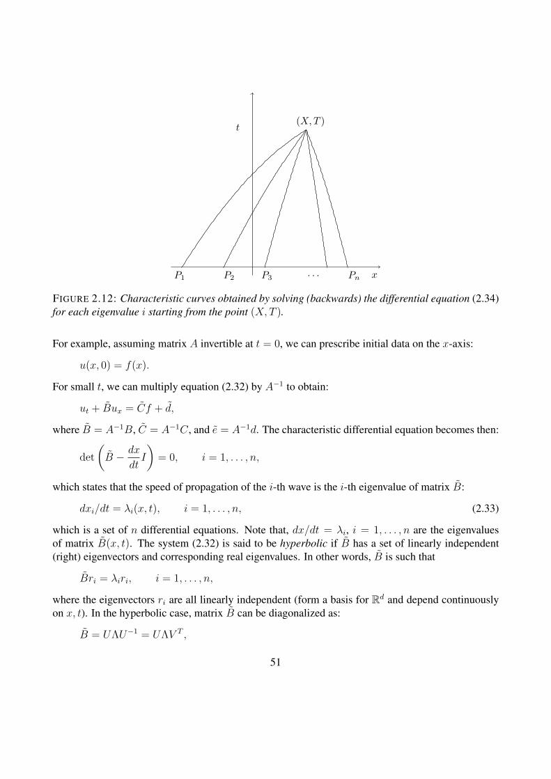
(X,T )t
xPn. . .P3P2P1
FIGURE 2.12: Characteristic curves obtained by solving (backwards) the differential equation (2.34)for each eigenvalue i starting from the point (X,T ).
For example, assuming matrix A invertible at t = 0, we can prescribe initial data on the x-axis:
u(x, 0) = f(x).
For small t, we can multiply equation (2.32) by A−1 to obtain:
ut + Bux = Cf + d,
where B = A−1B, C = A−1C, and e = A−1d. The characteristic differential equation becomes then:
det
(B − dx
dtI
)= 0, i = 1, . . . , n,
which states that the speed of propagation of the i-th wave is the i-th eigenvalue of matrix B:
dxi/dt = λi(x, t), i = 1, . . . , n, (2.33)
which is a set of n differential equations. Note that, dx/dt = λi, i = 1, . . . , n are the eigenvaluesof matrix B(x, t). The system (2.32) is said to be hyperbolic if B has a set of linearly independent(right) eigenvectors and corresponding real eigenvalues. In other words, B is such that
Bri = λiri, i = 1, . . . , n,
where the eigenvectors ri are all linearly independent (form a basis for Rd and depend continuouslyon x, t). In the hyperbolic case, matrix B can be diagonalized as:
B = UΛU−1 = UΛV T ,
51

where matrices U and V contain the ordered (with respect to the eigenvalues λi) right and left eigen-vectors ri and li as columns and the diagonal matrix Λ contains the corresponding eigenvalues λi(see Appendix D.3). Since U−1 = V T we can transform system (2.32) in canonical form by settingu = Uv, and thus v = V Tu, called the “characteristic variables”:
vt + Λvx = Cv + d,
with C = V TCU − V TUt − V TBUx and d = V Td. A few basic facts about linear algebra andleft and right eigenvectors are reviewed in Appendix D. Also the initial conditions are transformed:V Tf(x) = g(x) for t = 0. This way we have achieved a complete decomposition of the systemobtaining a set of first order differential equations for each component vi of the vector function v thatare coupled only on the right hand side. The i-th equation takes the form:
dvidt
=∂vi∂t
+dx
dt
∂vi∂x
=∂vi∂t
+ λi∂vi∂x
=n∑j=1
cijvj + di. (2.34)
Thus, we can use the method of characteristic to solve each equation obtaining a family of charac-teristics for each i = 1, . . . , n. The specific characteristic curve of the i-th family is obtained by“back-tracking”, i.e., solving the differential equation starting from a generic point (X,T ) to obtainpoints Pi on the x-axis (Figure 2.12). We would like to remark that the (qualitative) curves on the leftof point (X,T ) are relative to positive eigenvalues λi > 0, while the ones on the right correspond tonegative λi. Indicating with x(t) = γi(t,X, T ) the backtracked characteristic curve of the i-th family,the general solution of (2.34) is obtained by integration along the curve γi:
vi(X,T ) = gi(γi(0, X, T )) +
∫ T
0
(n∑j=1
cij(γi(τ,X, T ), τ)vj + di(γi(τ,X, T ), τ)
)dτ.
We remark here that the main difference that we note with respect to the scalar case is that now thei-th wave (in the new variables vi) is obtained as a superposition of all other waves vj , j = 1, . . . , ntraveling along different curves and with different characteristic speeds. In the integral above thedomain of integration changes with the wave number i, and for this reason in the coefficients cijand di the substitution x(τ) = γi(τ,X, T ) has been made where the curve γi is indexed with thewave number. We remark that, as seen in Section 2.2 for Burgers equation, the time interval wherethis solution is actually well defined cannot be too large, and we say that this solution is valid forsufficiently small T , usually without being more specific as done with Burgers equation.In the previous paragraphs we have looked at a pure initial value problem, where initial data wereprescribe at t = 0 on the entire x-axis. Now we want to consider the presence of a boundary. For thiswe assume that the equation is defined for x > 0, so that we need to impose a boundary conditionat x = 0 for all times t > 0. However, we have to specify these boundary conditions only forthose wave families corresponding to positive eigenvalues. For the other characteristic curves thedomain of dependence does not include the t-axis (Figure 2.12). If we rank the eigenvalues from the
52

(X,T )t
xPn. . .Pr
Pj
P1
FIGURE 2.13: Characteristic curves obtained by solving (backwards) the differential equation (2.34)for each eigenvalue i starting from the points (X,T ) and from the boundary point Pj .
smallest (λd) to the largest (λ1), i.e., λd < λd−1 < . . . < 0 < λr < λr−1 < . . . < λ1, we have thesituation shown in Figure 2.13, where from point Pj a new set of characteristics has been identifiedby backtracking. We recall again that all these qualitative considerations work only in the case ofsmooth solutions, when u is continuous together with its first derivative. In more complex situations,as we have seen for the Burgers equation where shocks develop, we can still proceed with a similaranalysis, but to do so we need to properly define how discontinuous solutions have to be interpreted.
Example 2.13. To exemplify the above development we address here the case of a system of firstorder PDEs with constant coefficients. Let u(x, t), f(x) ∈ Rd. Then our constant coefficient systemtakes the form:
ut + Aux = 0, u(x, 0) = f(x), (2.35)
where matrix A is a hyperbolic matrix, i.e., it has real eigenvalues and eigenvectors and is diagonal-izable. We denote by ri, li, λi the (constant) right and left eigenvectors and the eigenvalues of A,respectively, and as before we collect the right eigenvectors as columns of the matrix U and the lefteigenvectors as columns of the matrix V . Recalling (D.11), we can express the component of u usingthe basis U as ui = 〈li, u〉. Then scalar multiplication of (2.35) by l1, . . . , ld yields equations for thei-th wave:
〈li, ut〉+ 〈li, Aux〉 = ui,t + λiui,x = 0 ui(x, 0) = 〈li, f(x)〉 = fi(x).
We obtain a decoupled system of Cauchy problems that can be solved independently using the for-mula (2.3):
ui(x, t) = fi(x− λit).
53
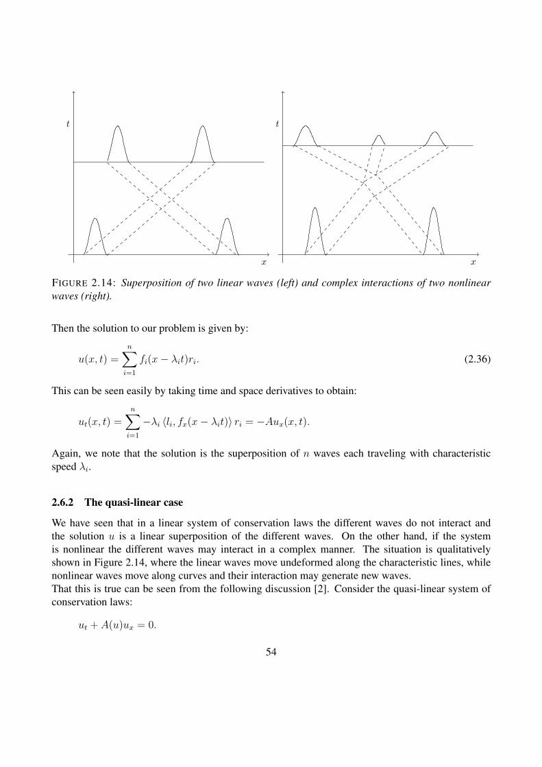
t
x
t
x
FIGURE 2.14: Superposition of two linear waves (left) and complex interactions of two nonlinearwaves (right).
Then the solution to our problem is given by:
u(x, t) =n∑i=1
fi(x− λit)ri. (2.36)
This can be seen easily by taking time and space derivatives to obtain:
ut(x, t) =n∑i=1
−λi 〈li, fx(x− λit)〉 ri = −Aux(x, t).
Again, we note that the solution is the superposition of n waves each traveling with characteristicspeed λi.
2.6.2 The quasi-linear case
We have seen that in a linear system of conservation laws the different waves do not interact andthe solution u is a linear superposition of the different waves. On the other hand, if the systemis nonlinear the different waves may interact in a complex manner. The situation is qualitativelyshown in Figure 2.14, where the linear waves move undeformed along the characteristic lines, whilenonlinear waves move along curves and their interaction may generate new waves.That this is true can be seen from the following discussion [2]. Consider the quasi-linear system ofconservation laws:
ut + A(u)ux = 0.
54

The matrix A(u) is a function of u and so are its eigenvalues λi(u) and its left and right eigenvectorsli(u) and ri(u). As usual we denote with U(u) = r1(u), . . . , rd(u) the matrix of the basis vectorsformed with the right eigenvectors, with V (u) = l1(u), . . . , ld(u) the matrix of the dual basis, i.e.the left eigenvectors, and with Λ(u) the diagonal matrix of the eigenvalues of A. Using (D.11), wecan express the spatial gradient∇u = ux as a linear combination of the right eigenvectors ri of A as:
ut = (V Tut)TU =
n∑i=1
〈li(u), ut〉 ri = −Aux = A(V Tux)TU = −
n∑i=1
λi(u) 〈li(u), ut〉 ri(u).
Differentiating ux with respect to t and ut with respect to x, equating the mixed derivatives, aftersome calculations (for details see [2]), we obtain:
(ux,i)t + (λiux,i)x =n∑
j=1,k=1j>k
Gijk, (2.37)
with Gijk given by:
Gijk = (λj − λk) 〈li, [rj, rk]〉ux,jux,k,
where [rj, rk] = Jrkrj − Jrjrk = [directional derivative of rk along rj]- [directional derivative or rjalong rk] is called the Lie bracket. The quantity Jrk denotes the Jacobian matrix of vector rj . There-fore, Jrkrj indicates the directional derivative of rk in the direction of rj . We note that equation (2.37)is in conservation form and decoupled on the left-hand-side. The source term, however, couples allthe waves. In fact, Gijk can be interpreted as the amount of i-waves originating from the interactionof j-waves with k-waves [2]. The quantity λj − λk describes the wave speed difference, the termux,jux,k the product of the densities of the j-waves and the k-waves, and 〈li, [rj, rk]〉 gives the i-thcomponent of the Lie bracket in the U basis .
2.7 Weak solutions for conservation lawsWe have seen that Burgers equation can be written in two ways:
ut + uux = 0 or ut +1
2(u2)x = 0.
The second form is actually called the conservation (or divergence) form. A general scalar conserva-tion equation in Rd is given by:
ut + divF (u,∇u) = 0, (2.38)
where the flux function F is an d-dimensional vector function F = (f1, f2, . . . , fd)T . In all generality,
we could assume our equation to be defined in a d-dimensional Euclidean subspace of Rd (usually
55

d = 1, 2 or 3), to which we could add the time as an extra coordinate t = xd+1, so that u ∈ Rd+1.Given a flux function F ∈ Rd, for simplicity assumed function only of u, we can add the timecomponent at the end of the vector elements, F (u) = (f1(u), f2(u), . . . , fd(u), u)T ∈ Rd+1. In thisway the conservation equation can be written as:
div F (u) = 0,
giving reason to the qualification of being “in divergence form” or a “conservation law”. In fact, givenany subset A of Rd+1 with regular boundary ∂A, the Gauss (or divergence) theorem states:∫
Adiv F (u)dx =
∫∂AF (u) · νds,
where ν is the unit outward normal to ∂A. Isolating t in the divergence, Gauss theorem can be writtenas: ∫
A
∂u
∂tdx+
∫∂AF (u) · ν ds = 0.
This is a conservation statement by which for any subset of the domain of definition of our PDE thesum of the fluxes exiting from or entering into A must equate the time variation of the total quantity(the integral) of u.For simplicity, from now on in this and the following sections we will restrict to one-dimensionalsystems of conservation laws of the type:
ut + f(u)x = 0, (2.39)
where u(x, t) : Ω 7→ R, Ω ∈ R×R is a bounded domain in the one-dimensional space (x) and time tspace, f(u) : R 7→ R is a smooth vector field, and the derivatives are taken component-wise. Higherdimensional problems can be treated numerically by extensions of the one-dimensional counterpart.We should stress that a complete theory of nonlinear hyperbolic conservation systems is still missing,while for the one-dimensional case many more results are available. Many of the numerical tools thatwe will develop later on rely heavily on the theory for the one-dimensional case, by extending therelative concepts to multi-dimensions, even if no theory support their use. The success obtained bythese numerical schemes is an indication that the fundamentals are correct, even though difficultiesstill remain in particular for nonlinear systems of conservation laws.Returning to the one-dimensional case, we note that the use of the divergence theorem in (2.39) isnothing else than a simple application of the fundamental theorem of calculus. Indeed, integratingover a generic interval [a, b] contained in the domain of the equation we get:
d
dt
∫ b
a
udx =
∫ b
a
utdx
= −∫ b
a
f(u(x, t))xdx = f(u(a, t))− f(u(b, t))
= INFLOW (in a) - OUTFLOW (in b).
56

Again this is a conservation statement: the rate of change of the total quantity of u in [a, b] is equal toinflow - outflow. The use of the fundamental theorem of calculus in this setting is nothing else thanthe application of the divergence theorem, as the boundary of the interval [a, b] if formed by the pointsx = a and x = b and there the normals are the scalars −1 and 1, respectively.If the solution u is regular (sufficiently continuous), then the scalar equation (2.39) is equivalent to:
ut + a(u)ux = 0,
where a(u) = f ′(u) is the derivative of f . We can see that if u is discontinuous, say at a point ξ, itsderivative is not defined. Actually it can be defined in a distributional sense and then it will contain aDirac mass in ξ. In any case, its product with the discontinuous function a(u) is not well defined. Onthe other hand, the use of equation (2.39) is always meaningful. This is a strong reason for using theconservation form of the equation.A sensible approach for the definition of a solution that can be discontinuous is to use integrals andtry to avoid differentiation. To this aim, similarly to what is done for elliptic problems, we multiplyour equation by a test function φ(x, t) ∈ C1
c , i.e., a function that is continuous and differentiable ina compact support 5. In our case, we can take a continuous function that is nonzero in a boundedinterval [α, β] ∪ [t, t + ∆t] and is zero outside. Then we integrate in the support of φ (outside thesupport the integral will be zero), and integrate in time:∫ t+∆t
t
[∫ β
α
(ut + f(u)x)φ(x, τ)dx
]dτ = 0.
Then we apply integration by parts in the outer and inner integrals and use the fact that the boundaryterms of vanish because φ is zero outside its support to obtain:
−∫ t+∆t
t
(∫ β
α
u(x, τ)∂
∂tφ(x, τ) + f(u(x, τ))
∂
∂xφ(x, τ)dx
)dt = 0.
Now everything is well defined, as φt and φx are the only derivatives that appear in the expression.Then we say that a locally integrable function u(x, t) is a “weak solution” of equation (2.39) if:∫ t+∆t
t
∫ β
α
(uφt + f(u)φx)dxdτ = 0, (2.40)
holds for every function φ(x, t) ∈ C1c . From the fundamental lemma of calculus of variations, if the
previous equation is satisfied for every nonzero differentiable function with compact support, thenthere is a statement of equivalence between this formulation and the integral formulation involvingthe derivatives of u. Obviously, if u is continuous, then the two formulations (2.39) and (2.40) areequivalent. In fact we can write:∫ ∫
(uφt + f(u)φx) =
∫ ∫(utφ+ f(u)xφ) =
∫ ∫(ut + a(u)ux)φ = 0 for all φ ∈ C1
c ,
5The support of a function is the set where the function is nonzero
57

t
x
ΩRΩL
νL
νR
x− λt = 0
u = uR
u = uL
Supp φ
u
x
λ
f ′(u)
FIGURE 2.15: Exemplification of piecewise constant function with jump discontinuity on a charac-teristic line (left). Interpretation of the Rankine-Hugoniot condition for the scalar case (right).
which yields:
ut + a(u)ux = 0.
2.7.1 Jump conditions
In this section we consider a system of the form (2.39) and look at conditions that need to be satisfiedby the weak solution u(x, t) so that it is well defined. We first consider a simple example of apiecewise constant U that jumps from uL ∈ Rd to uR ∈ Rd across the characteristic line x = λt.Then we can write:
U(x, t) =
uL if x > λt,
uR if x < λt,(2.41)
The situation is depicted in Figure 2.15 (left). The characteristic curve divides Ω in a left and a rightportion:
ΩL = Ω ∩ x > λt ΩR = Ω ∩ x < λt.
We look for weak solutions as defined in the previous Section. Hence let φ(x, t) be a test function withlocal support (the region bounded by the dashed line in Figure 2.15, left) that is sufficiently regularfor the purposes and such that φ = 0 in ∂(Supp (φ)). For brevity, we do not indicate the limits ofthe time integration, with the understanding that we are integrating in a bounded interval included in
58

[0, T ]. We form the augmented vector field w = (f(U)φ, Uφ), adding the time as the last componentof our space, and use it in equation (2.40) to obtain:∫
Ω
(Uφt + f(U)φx) dx dt =
∫ΩL
divw dx dt+
∫ΩR
divw dx dt = 0
Note that the outward unit normals to Ωl and Ωr are given by:
νR = (−1,−λ) νL = (−1, λ), (2.42)
so that application of the divergence theorem yields:∫Ω
divw dx dt =
∫∂ΩR
⟨w, νR
⟩ds+
∫∂ΩL
⟨w, νL
⟩ds = 0,
since φ = 0 in ∂Ω. Using (2.42) and the expression for w we obtain:∫ (λuR − f(uR)
)φ(t, λt) dt+
∫ (λuL − f(uL)
)φ(t, λt) dt = 0,
or rearranging terms:∫ [λ(uR − uL)
]−[f(uR)− f(uL)
]φ(t, λt) dt = 0.
Since this must hold true for every φ, we conclude:
λ(uR − uL) = f(uR)− f(uL),
which is called the “Rankine-Hugoniot” jump condition. In practice, this condition states that a weaksolution of the system of conservation laws (2.39) must satisfy the Rankine-Hugoniot condition. Thecondition can be restated by saying that the “average” speed of the shock (or discontinuity) times thejump in the state must equate the jump in the flux. Note that the flux difference is nothing else thanthe conservation statement for the conserved quantity u across the characteristics. Then, the Rankine-Hugoniot condition states that the flux difference at a point (τ, ξ) on the characteristics must be equalto the average velocity times the state difference.In fact, for a scalar equation it is easy to interpret λ as an average speed. Indeed:
λ =f(uR)− f(uL)
uR − uL =1
uR − uL∫ uR
uLf ′(s) ds =
1
uR − uL∫ uR
uLa(s) ds =
Figure 2.15, (right) gives an intuitive graphic interpretation.There is another way to determine the Rankine-Hugoniot conditions related to a topic we will see inthe numerical approach in the next sections. Denote by A(u) = J f(u) the Jacobian matrix of f(u).Define an “average” matrix with a parameter θ ∈ [0, 1] and such that A(u, u) = A(u):
A(uL, uR) =
∫ 1
0
A(θuL + (1− θ)uR
)dθ, (2.43)
59
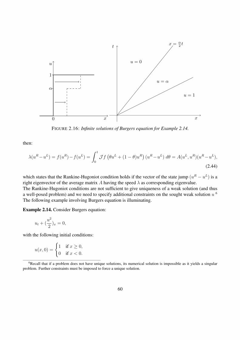
x
u
1
α
0 x
tx = α
2 t
u = α
u = 0
u = 1
FIGURE 2.16: Infinite solutions of Burgers equation for Example 2.14.
then:
λ(uR−uL) = f(uR)−f(uL) =
∫ 1
0
J f(θuL + (1− θ)uR
)(uR−uL) dθ = A(uL, uR)(uR−uL),
(2.44)
which states that the Rankine-Hugoniot condition holds if the vector of the state jump (uR − uL) is aright eigenvector of the average matrix A having the speed λ as corresponding eigenvalue.The Rankine-Hugoniot conditions are not sufficient to give uniqueness of a weak solution (and thusa well-posed problem) and we need to specify additional constraints on the sought weak solution u 6
The following example involving Burgers equation is illuminating.
Example 2.14. Consider Burgers equation:
ut + (u2
2)x = 0,
with the following initial conditions:
u(x, 0) =
1 if x ≥ 0,
0 if x < 0.
6Recall that if a problem does not have unique solutions, its numerical solution is impossible as it yields a singularproblem. Further constraints must be imposed to force a unique solution.
60

The function:
uα(x, t) =
0 if x < α
2t
α if α2t < x < 1+α
2t
1 if x ≥ 1+α2t
is a weak solution of our problem, as it is a piecewise constant function and satisfies the Rankine-Hugoniot condition
λ(urα − ulα) =
(urα2
)2
−(urα2
)2
,
along the characteristic lines:
x(t) =α
2t and x(t) =
1 + α
2t.
Since this is valid for every 0 ≤ α ≤ 1, we have infinite solutions to this problem.
In the following paragraphs we want to find additional constraints so that we can identify a uniquesolution among the possible infinite ones. We will see that there are a number of these conditions,many are equivalent, and we need to make a choice. We will describe the most relevant for ourpurposes.
2.7.2 Admissibility conditions
There are three main approaches to impose enough constraints to force the weak solution to be unique:“Viscosity solutions”, “Entropy conditions”, and “Stability conditions”. We follow again [2] and callthese conditions “admissibility conditions”.
Viscosity solutions or Vanishing viscosity. In this approach we add a “viscosity” term to our con-servation law, and we look for solutions at the limit of “zero” viscosity. Hence, given a positive ε, wereformulate the problem as:
uεt + f(uε)x = εuεxx, (2.45)
and look for the limit as ε 7→ 0+. Thus we say that a weak solution u(x, t) is “admissible in thevanishing viscosity sense” if uε(x, t) 7→ u(x, t) as ε 7→ 0.This approach is usually consistent, as most conservation laws are physically obtained by assumingdissipation (a term typically proportional to the second derivative) to be negligible. However, thiscondition is difficult to assess in practice, and has mostly a theoretical use.
61

Entropy conditions. This admissibility condition takes origin from the observation that in thermo-dynamically dissipative systems the entropy is never decreasing and if the system is non-dissipativethen entropy is conserved. Hence we look for a scalar function S of the system state vector u and saythe entropy S(u) and the entropy flux q(u) should obey a conservation law.We say that a scalar function S(u) : Rd 7→ R is called the “entropy” associated with the system ofconservation laws (2.39) with corresponding entropy flux q(u) : Rd 7→ R if they satisfy:
J f(u)∇S(u) = A(u)∇S(u) = ∇ q(u). (2.46)
For such a function, we have:
S(u)t + q(u)x = 〈∇S(u), ut〉+ 〈∇ q(u), ux〉 = 〈∇S(u), (ut + Juf(u)ux)〉 = 0, (2.47)
showing that entropy is conserved. This is true for continuous solutions, but not so if discontinuitiesare present, as the following example shows.
Example 2.15. For Burgers equation with flux f(u) = u2/2, we can define an entropy functionS(u) = u3 and the corresponding entropy flux q(u) = 3/4u4. An easy calculation shows that theysatisfy the defining condition (2.46). We consider the piecewise constant weak solution for Burgersequation given by:
u(x, t) =
uL = 1 if x < t/2,
uR = 0 if x ≥ t/2.
Given this solution, the Rankine-Hugoniot condition for equation (2.47) is not satisfied. Indeed, sincethe shock speed is λ = 1/2, we have:
3
4
(q(uR)− q(uL)
)6= λ
(S(uR)− S(uL)
)=
1
2.
If we multiply equation (2.45) by∇S and using the definition of entropy function, we have 7:
S(uε)t + q(uε)x = ε∇S(uε)uεxx = ε [S(uε)xx − Jx(∇S(uε)) · uxx] .
The last term in the square brackets is always positive if S is a convex function. Multiplying by apositive and smooth test function φ with compact support and integrating by parts we have:∫ ∫
[S(uε)φt + q(uε)φx] dxdt ≥ −ε∫ ∫
S(uε)φxx dxdt.
7We note that
(S(u))xx = (∇S · ux)x = Jx(∇S) · ux +∇S · uxx.
62

x
u
ur
u∗
ul
x
u
ul
u∗
ur
FIGURE 2.17: The solution to this problem is stable if the wave that stays behind has a speed that islarger or equal than the speed of the wave ahead.
If uε 7→ u as ε 7→ 0 we have:∫ ∫S(u)φt + q(u)φx dxdt ≥ 0
for φ > 0. Again using integration by parts we can show that the previous statement implies S(u)t +q(u)x ≤ 0.Hence we say that a weak solution u(x, t) of (2.39) is “entropy admissible” if:
S(u)t + q(u)x ≤ 0.
Using the divergence theorem, it can be shown that the previous inequality holds if and only if:
λ[S(uR)− S(uL)
]≥ q(uR)− q(uL).
Stability (Liu) conditions. We start from a scalar nonlinear conservation law. Consider a piecewiseconstant weak solution jumping from uL to uR across the characteristics (as in (2.41)). We perturb ourproblem by adding an intermediate state uL ≤ u∗ ≤ uR (or vice-versa). Then the shock is subdividedinto two parts moving with speed given by the Rankine-Hugoniot conditions (see Figure 2.17). Thedistance between the waves of the original and the perturbed problems does not increase in time onlyif the speed of the shock behind is larger or equal to the speed of the shock ahead. This is obtained ifand only if:
f(u∗)− f(uL)
u∗ − uL ≥ f(uR)− f(u∗)
uR − u∗ for all u∗ ∈ [uL, uR].
The previous equation identifies secant lines in the graph of f(u). In practice, if uL < uR the graphof f should remain above the secant line (Figure 2.18, left), while if uL > uR the graph of f shouldstay below. This must hold also for any internal state u∗ ∈ [uL, uR].
63
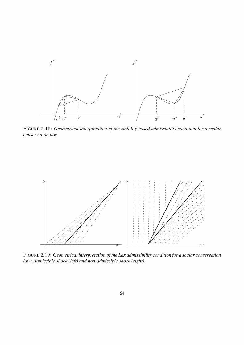
u
f
ul u∗ ur u
f
ul u∗ ur
FIGURE 2.18: Geometrical interpretation of the stability based admissibility condition for a scalarconservation law.
x
t
x
t
FIGURE 2.19: Geometrical interpretation of the Lax admissibility condition for a scalar conservationlaw: Admissible shock (left) and non-admissible shock (right).
64

In the case of systems, the situation is obviously more complicated. In practice stability implies thatthe same statement holds for any intermediate condition u∗. In other words, a shock with left and rightstates given by uL and uR satisfies the admissibility condition if its speed is less than or equal to thespeed of every smaller shock connecting uL with u∗. This condition due to Liu [10] has been shownto identify solutions equivalent to viscosity solutions and is called the Liu admissibility condition.
Lax admissibility conditions. A final admissibility criterion due to Lax [8] must be mentionedbecause of its wide spread use in the numerical solution of systems of conservation laws. A shock ofthe i-th family is said to satisfy the “Lax admissibility criterion” if it moves with a speed λi(uL, uR)such that:
λi(uL) ≥ λi(u
L, uR) ≥ λi(uR).
Consider again a piecewise smooth (constant) weak solution u(x, t) of our system with a discontinuityalong the curve x = γ(t), across which u assumes the left and right states uL and uR. The i-th wavemust travel with a speed dx/dt = γ(t) = λi(u
L, uR) given by the i-th eigenvalue of the averagematrix A(uL, uR) defined in (2.43). This requires that the characteristic lines run into the shock linefrom both sides. The geometrical interpretation is reported in Figure 2.19 showing on the left panelan admissible shock and on the right panel a non-admissible one.
2.8 The Riemann Problem.This section is again taken from [2]. For more details and applications see [9, 12]. Let’s start byposing the problem in all generality.
Problem 2.16 (Riemann Problem). Find the function u(x, t) weak solution in the sense of (2.40) ofsystem of conservation laws::
ut + f(u)x = 0, x ∈ Ω = [−δ,+δ],
with piecewise constant initial conditions:
u(x, 0) =
uL if x < 0,
uR if x > 0.
Solutions to Riemann problems arise both in the theoretical analysis of hyperbolic conservation lawsand in their numerical solution. From what we have seen so far, it is clear we can construct the globalsolution of a system of conservation laws by gluing together solutions to local (point-wise) Riemannproblems starting from the initial data. Intuitively, these initial data define the appropriate left andright states uL and uR on the x axis to initialize a sort of explicit time-stepping scheme that can beused to define the solution u(x, t) on the entire spatial domain after a sufficiently small time step ∆t.
65

x0
λ
uL
uR u(t)
λt
FIGURE 2.20: Example 2.17. Riemann problem solution for the advection of a contact discontinuity.
The Riemann problem can be used effectively as a replacement of the global conservation law in alocal approximation whereby the characteristics can be assumed constant and hence generated by theright eigenpairs of the Jacobian matrix. It is intuitive but can be proved formally that this can be doneas long as the left and right states uL and uR are close to each other. In other words, we may thinkthat to obtain the global solution we just put together solutions to Riemann problems defined at a setof points xi, i = 1, . . . as long as ∆x = xi+1 − xi is not too large (so that linearization of the originalproblem is accurate) and we advance in time for a sufficiently small step ∆t. It can be proved thatglobal solutions can be obtained in this manner by letting ∆x and ∆t tend to zero.We note that we have to define a number of Riemann problems at different values of x, so that wewould like that the Riemann problem be independent of the location of the reference frame. Indeed,we directly observe that the solution of the Riemann problem is invariant under linear transformationof the variables, i.e., given θ > 0:
u(x, t) = u(θx, θt),
Once the solution of the Riemann problem 2.16 is found, then the previous transformation can beused to define the solution at every x and t given the appropriate initial data. We work out in detailssome simple examples that clarifies the situation, referring to [2, 12] for more general developments.
Example 2.17. Consider the following scalar problem with a linear flux function:
ut + λux = 0.
The propagation speed is f ′(u) = λ and the solution of the Riemann problem is:
u(x, t) =
uL if x < λt,
uR if x > λt.
This solution is a single jump called a “contact discontinuity” traveling with speed λ (Figure 2.20).
Example 2.18. Consider the following scalar problem with a convex flux function (e.g. f(u) = u/2)and initial data such that uR > uL:
ut + (u2
2)x = 0.
66
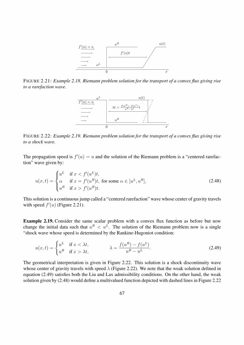
x0
f ′(u) = u
uL
uR u(t)
f ′(u)t
FIGURE 2.21: Example 2.18. Riemann problem solution for the transport of a convex flux giving riseto a rarefaction wave.
x0
f ′(u) = uuL
uR
u(t)
λt = f(uR)−f(uL)uR−uL t
FIGURE 2.22: Example 2.19. Riemann problem solution for the transport of a convex flux giving riseto a shock wave.
The propagation speed is f ′(u) = u and the solution of the Riemann problem is a “centered rarefac-tion” wave given by:
u(x, t) =
uL if x < f ′(uL)t,
α if x = f ′(uR)t, for some α ∈ [uL, uR],
uR if x > f ′(uR)t.
(2.48)
This solution is a continuous jump called a “centered rarefaction” wave whose center of gravity travelswith speed f ′(u) (Figure 2.21).
Example 2.19. Consider the same scalar problem with a convex flux function as before but nowchange the initial data such that uR < uL. The solution of the Riemann problem now is a single“shock wave whose speed is determined by the Rankine-Hugoniot condition:
u(x, t) =
uL if x < λt,
uR if x > λt,λ =
f(uR)− f(uL)
uR − uL . (2.49)
The geometrical interpretation is given in Figure 2.22. This solution is a shock discontinuity wavewhose center of gravity travels with speed λ (Figure 2.22). We note that the weak solution defined inequation (2.49) satisfies both the Liu and Lax admissibility conditions. On the other hand, the weaksolution given by (2.48) would define a multivalued function depicted with dashed lines in Figure 2.22
67
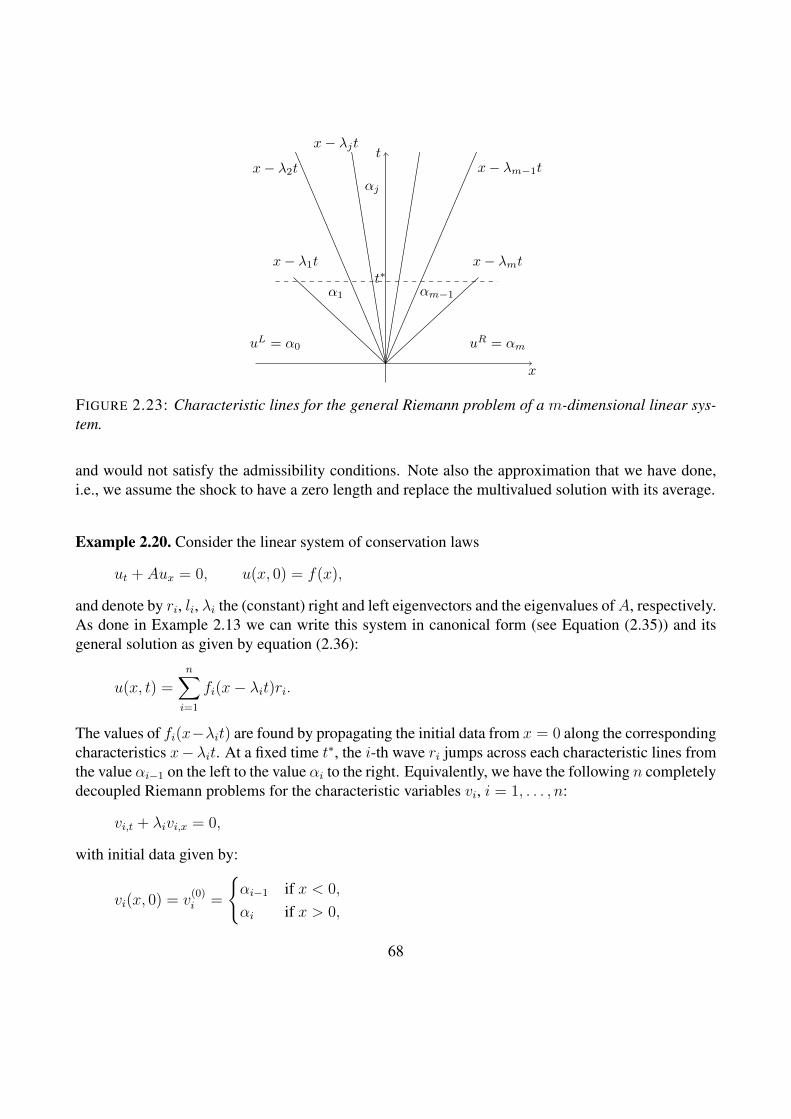
x
t
uL = α0
α1
αj
αm−1
uR = αm
x− λ1t
x− λ2tx− λjt
x− λm−1t
x− λmtt∗
FIGURE 2.23: Characteristic lines for the general Riemann problem of a m-dimensional linear sys-tem.
and would not satisfy the admissibility conditions. Note also the approximation that we have done,i.e., we assume the shock to have a zero length and replace the multivalued solution with its average.
Example 2.20. Consider the linear system of conservation laws
ut + Aux = 0, u(x, 0) = f(x),
and denote by ri, li, λi the (constant) right and left eigenvectors and the eigenvalues ofA, respectively.As done in Example 2.13 we can write this system in canonical form (see Equation (2.35)) and itsgeneral solution as given by equation (2.36):
u(x, t) =n∑i=1
fi(x− λit)ri.
The values of fi(x−λit) are found by propagating the initial data from x = 0 along the correspondingcharacteristics x−λit. At a fixed time t∗, the i-th wave ri jumps across each characteristic lines fromthe value αi−1 on the left to the value αi to the right. Equivalently, we have the following n completelydecoupled Riemann problems for the characteristic variables vi, i = 1, . . . , n:
vi,t + λivi,x = 0,
with initial data given by:
vi(x, 0) = v(0)i =
αi−1 if x < 0,
αi if x > 0,
68

x
u = Si(σ)(u0)
u = Ri(σ′)(u0)
ri(u0)u0
FIGURE 2.24: Definition of the i-th integral (shock) curve through a point u0 using the left eigenval-ues (equation (2.51), solid line) and using the differential equation (2.52) (dotted line).
the solution of which is given by:
vi(x, t) = v(0)i (x− λit) =
αi−1 if x− λit < 0,
αi if x− λit > 0.
Since the right eigenvectors are linearly independent, we can write the left and right initial conditionsas linear combinations of these vectors:
uL =n∑i=1
αi−1ri, uR =n∑i=1
αiri.
At a point (x, t) there exist a value I of the index i such that x − λIt > 0 for i ≤ I . Thus the finalsolution is given by:
u(x, t) =n∑
i=I+1
αi−1ri +I∑i=1
αiri.
The general structure of the set of characteristic lines of this system is described geometrically inFigure 2.23.
2.8.1 Shock and rarefaction curves
In the previous section we have seen waves named “contact discontinuities”, “rarefactions”, and“shocks”. We would like to describe in somewhat more details what these waves are and in whichproblems they arise. In practice, we need to be able to construct the discontinuity curves. To this aim,we start from a point uo ∈ Rd and try to find the state vector u that satisfies the Rankine-Hugoniotequations (2.44):
λ(u− u0) = f(u)− f(u0) = A(u0, u)(u− u0).
69

Obviously, the trivial identity is obtained for u = u0. We want to find a different solution in aneighborhood of u0. We note that this is a n-dimensional nonlinear system with n + 1 unknowns(u, λ) and cannot be solved as is.The bi-orthogonality condition of the left and right eigenvalue systems of A(u0, u) yields:
〈lj(u0, u), (u− u0)〉 = 0 for all j 6= i, i = 1, . . . , n (2.50)
This is a n − 1-dimensional nonlinear system in the n unknowns given by the components of u. Wecan linearize this system by noting that by definition of average matrix (2.43) A(u0, u0) = A(u0), andhence we can write the following n− 1-dimensional linear system:
〈lj(u0), (u− u0)〉 = 0 for all j 6= i.
Because of the bi-orthogonality condition, the previous equation tells us that the vector u − u0 mustbe perpendicular to all the left eigenvectors lj j 6= i, and thus parallel to ri:
u = u0 + αri(u) for all i.
Thus, the state vector u along a shock curve must be tangent to the curve, or stated in a different way,the solution to (2.50) is a smooth curve tangent to i-th eigenvector ri of the Jacobian matrix A(u0) atu0, a condition that gives us a (inconvenient but) practical way to calculate the curve given u0. Thus,at least in principle, the equation of the characteristic curve can be written in parametric form withparameter σ as:
u = Si(σ)(u0). (2.51)
We note that the curve at each point σ must be orthogonal to li and tangent to ri (see Figure 2.24).On the other hand, we can define the “i-th rarefaction curve” as the integral curve of the vector fieldri(u) passing through u0. In other words, to determine the i-th rarefaction curve we can define adifferential equation in parametric space imposing the tangent condition on the right eigenvalue:
du
dσ= ri(u), u(0) = u0.
The solution to this equation gives a curve (again in parametric space):
u = Ri(σ)(u0), (2.52)
which results close to the shock curve u = Si(σ)(u0) up to second order around u0 (Figure 2.24).Hence, at least locally around u0 we can confound Si(σ)(u0) with Ri(σ)(u0). In fact, the followingresult can be proved:
Ri(σ)(u0) = u0 + σri(u0) +O(σ2)
Si(σ)(u0) = u0 + σri(u0) +O(σ2),
70
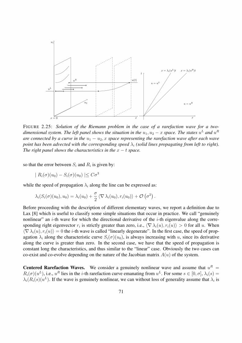
x
u1
u2
x = 0
uL
uR u(t)
x
tx = λi(u
L)t x = λi(uR)t
u = uL
u = uR
FIGURE 2.25: Solution of the Riemann problem in the case of a rarefaction wave for a two-dimensional system. The left panel shows the situation in the u1, u2 − x space. The states uL and uR
are connected by a curve in the u1 − u2, x space representing the rarefaction wave after each wavepoint has been advected with the corresponding speed λi (solid lines propagating from left to right).The right panel shows the characteristics in the x− t space.
so that the error between Si and Ri is given by:
| Ri(σ)(u0)− Si(σ)(u0) |≤ Cσ3
while the speed of propagation λi along the line can be expressed as:
λi(Si(σ)(u0), u0) = λi(u0) +σ
2〈∇λi(u0), ri(u0)〉+O
(σ2).
Before proceeding with the description of different elementary waves, we report a definition due toLax [8] which is useful to classify some simple situations that occur in practice. We call “genuinelynonlinear” an i-th wave for which the directional derivative of the i-th eigenvalue along the corre-sponding right eigenvector ri is strictly greater than zero, i.e., 〈∇λi(u), ri(u)〉 > 0 for all u. When〈∇λi(u), ri(u)〉 = 0 the i-th wave is called “linearly degenerate”. In the first case, the speed of prop-agation λi along the characteristic curve Si(σ)(u0), is always increasing with u, since its derivativealong the curve is greater than zero. In the second case, we have that the speed of propagation isconstant long the characteristics, and thus similar to the “linear” case. Obviously the two cases canco-exist and co-evolve depending on the nature of the Jacobian matrix A(u) of the system.
Centered Rarefaction Waves. We consider a genuinely nonlinear wave and assume that uR =Ri(σ)(uL), i.e., uR lies in the i-th rarefaction curve emanating from uL. For some s ∈ [0, σ], λi(s) =λi(Ri(s)(u
L). If the wave is genuinely nonlinear, we can without loss of generality assume that λi is
71

increasing with s and is injective (for each value of λ ∈ [λi(uL), λi(u
R)] there is a unique value of ssuch that λ = λi(s)). The solution of the Riemann problem is then given by:
u(x, t) =
uL if x < λi(u
L)t,
Ri(s)(uL) if x = λi(s)t, λi(s) ∈ [λi(u
L), λi(uR)],
uR if x > λi(uR)t.
Figure 2.25 summarizes the behavior. The construction of the solution u(x, t) for a fixed time tproceeds as follows. The rarefaction wave at x = 0 connecting the left and right states uL and uR isdrawn on the spanning u and passing through x = 0 (shown in the figure with a dotted curve). Eachpoint of this curve is moved horizontally by the amount λi(u)t.
Shock Waves. We look now at the case in which the uR state is connected t the uL state by a shockcurve uR§i(σ)(uL). This occurs if the system is genuinely nonlinear. We can define the Rankine-Hugoniot speed λ = λi(u
R, uL). The (piecewise constant) solution to the Riemann problem is then:
u(x, t) =
uL if x < λt
uR if x > λt.
Note that for σ > 0, we have that λi(uR) > λi(uL) and thus the Lax admissibility condition is
violated. Obviously, the Lax condition is satisfied, i.e., u(x, t) is “entropy-stable” for σ < 0 sincethen λi(uR) < λi(u
L, uR) < λi(uL).
Contact Discontinuity Waves. A contact discontinuity occurs for a linearly degenerate wave field.Let uR = Ri(σ)(uL), i.e., the states uL and uR lie on a rarefaction curve, along which the speedis a constant (by assumption intrinsic in the Riemann problem formulation). The Rankine-Hugoniotcondition writes:
f(uR)− f(uL) =
∫ σ
0
Jff(Ri(s)(u
L))ri(Ri(s)(u
L))ds
=
∫ σ
0
λi(uL) ri
(Ri(s)(u
L))ds
= λi(uL)[Ri(σ)(uL)− uL
].
The Lax entropy condition is satisfied as λi(uL) = λi(uL, uR) = λi(u
R) and, moreover, the shockand rarefaction curves coincide Si(σ)(uL) = Ri(σ)(uL) for all σ.The three elementary wave types are exemplified by the graphs in Figure 2.26 drawn in the x − tplane. The structure of the different waves can be identified by the direction of the left and rightcharacteristics (drawn as dashed arrows) that are converging towards the discontinuity line in the caseof a shock, parallel to the discontinuity line in the case of a contact discontinuity, and parallel to theleft and right characteristics lines external to the rarefaction fan.
72

x
tx = λit
u = uL
u = uR
x
tx = λit
u = uL
u = uR
x
tx = λi(u
L)t x = λi(uR)t
u = uL
u = uR
FIGURE 2.26: Qualitative behavior of the characteristic fields for the three types of elementary wavesused in the solution of the Riemann problem: shock (left), contact discontinuity (center), rarefaction(right). The dash arrows indicate the directions of the characteristic curves outside the discontinuityregion.
General solution of the Riemann problem The general solution of the Riemann problem can nowbe obtained as a superposition of elementary waves. To this aim, we want to find intermediate statesuL = α0, α1, . . . , αd = uR such that each pair of adjacent states can be connected by one of thepreviously described elementary waves. In mathematical terms we can say that the intermediate stateαi is connected to the previous state αi−1 via a curve αi = Ψi(σi)(αi−1), so that the uL and uR statescan be written as a composition of the d functions:
uR = Ψd(σd) . . .Ψ1(σ1)(uL).
If uR and uL are not too far apart, it can be shown that the above equation is well-posed and that thereexist unique values of the wave strengths σi such that the above equation holds. Hence we proceedby starting from the uL = α0 state and solve a sequence of Riemann problems for i = 1, . . . , n:
ut + f(u)x = 0 u(x, 0) =
αi−1 if x < 0,
αi if x > 0,
as seen for example in the case of a linear system in Figure 2.23. Each of the Riemann problems hasan entropy solution in the i-th characteristic family.
3 Numerical Solution of Hyperbolic Conservation LawsIn this section we used the previous developments to work the details of numerical schemes for thesolution of Hyperbolic Conservation Laws. We will address essentially the method of Finite Volumesand digress only shortly on the Discontinuous Galerkin method, without touching at all the importantfield of purely Lagrangian methods.
73
We will be using most of the theoretical developments described in the previous sections as funda-mental building blocks for our numerical approach. We will focus on standard finite volume schemesmaintaining and discussing as much as possible multidimensional problems. However, as truly mul-tidimensional methods are still open questions, we will spend much time looking at one-dimensionalapproximations, but we will try to use multidimensional approximations. For the more recent devel-opments we refer the reader to more specialized books.
3.1 The Differential EquationProblem 3.1. Given a domain Ω ∈ Rd, which we assume possesses sufficient regularity, we want tofind a vector function u ∈ Rm, u = (u1, . . . , um), ui = uu(x, t) : Ω × R+ 7→ R, that satisfies thefollowing equation:
ut + div f(u) = 0 for all x ∈ Ω and t ∈ [0, T ], (3.1)u(x, 0) = u0 for all x ∈ Ω and t = 0, (3.2)u(0, t) = ub for all x ∈ ∂Ωin and t ∈ [0, T ], (3.3)
where f(u) = (f1(u), . . . , fd(u)), fi(u) : Rm 7→ Rm.
We notice here that the ”inflow” boundary where boundary conditions are imposed must satisfy thecompatibility conditions discussed in section 2.3. We start by giving some basic definitions of thedomain discretizations and its property and define the geometric quantities that will be needed in thedevelopment.
3.2 The Finite Volume Method3.2.1 Preliminaries
There are different equivalent ways to develop the Finite Volume Method. Our approach is to relymainly on Gauss (or Divergence) theorem and the derived integration by parts (Green’s Lemma) inorder to always focus on the conservation principle that is the foundation of the models of interest. Werecall here the most important mathematical results that will be of use in our developments, remindingto standard analysis books for the details of the proofs.
Theorem 3.1 (Gauss or Divergence). Given a subset Ω ∈ Rd having piecewise smooth boundaryΓ = ∂Ω, and a continuously differentiable (C1(Ω)) vector field F (x) ∈ Ω, we have:∫
Ω
divF dx =
∫Γ
F · ν ds, (3.4)
where ν is the outward unit normal to Γ, dx denotes the volume (surface) measure on Ω and ds thesurface measure on Γ and v · w = 〈v, w〉 denotes the scalar product between vectors v, w of Rd.
74
Theorem 3.2 (First Green Identity – Green’s Lemma). Let v, w ∈ Rd be piecewise continuous vectorfields and let Ω and Γ as in the previous theorem, then:∫
Ω
∇ v · ∇w dx =
∫Γ
v ∇w · ν ds−∫
Ω
v div∇w dx, (3.5)
where div∇ = ∆ is Laplace differential operator of second derivatives.
Remark 3.2. In (3.4) the left-hand-side contains the sum of the partial derivatives of the vector fieldF , and for this reason the hypothesis of the theorem contains the requirement that F be continuouslydifferentiable. The right-hand-side, on the other hand, does not contain any derivative, and thus inprinciple the integral of the fluxes over the subset Ω could be defined without the requirement thatF be C1. However, the normal to the surface Γ must be well-defined and this is the reason for therequirement that Γ be piecewise smooth. In fact, if the boundary Γ is formed by the union of msmooth surfaces that intersect at boundaries that form C1 curves, i.e.:
Γ =m⋃i=1
Γi γij(t) = Γi ∩ Γj ∈ C1 for all i and j, then∫
Γ
=m∑i=1
∫Γi
.
The same argumentation can be made, with the appropriate changes, for Green’s Lemma 3.5.The Finite Volume (FV) scheme can be derived by the following operations:
1. partition the domain Ω into M polygonal “finite volumes” or cells Ti, i = 1, . . . ,M (see nextparagraph for a complete definition of cells);
2. integrate equation (3.1) in time and space over the domain Ω and the time interval [tk, tk+1]:∫ tk+1
tk
(∫Ω
ut + div f(u) dx)
dt = 0;
3. use the linearity property of the integration to write:∫ tk+1
tk
(∫Ω
ut + div f(u) dx)
dt =M∑i=1
∫ tk+1
tk
(∫Ti
ut + div f(u) dx)
dt = 0;
impose that each term of the sum is zero:∫ tk+1
tk
∫Ti
(ut + div f(u) dx) dt = 0 i = 1, . . . ,M ;
4. apply the divergence theorem and use the fact that the cells are of polygonal shape:∫ tk+1
tk
(∫Ti
ut dx+
∫∂Ti
f(u) · ν dx)
dt =∫ tk+1
tk
(∫Ti
ut dx+Nσ∑j=1
∫σij
f(u) · νj ds
)dt = 0 i = 1, . . . ,M ;
75

5. exchange the first space integral with the time integral (the functions are assumed to be contin-uous and the domain of integration is assumed to be constant):∫
Ti
∫ tk+1
tkut dt dx+
∫ tk+1
tk
(Nσ∑j=1
∫σij
f(u) · νj ds
)dt = 0 i = 1, . . . ,M ;
6. integrate the first addendum in time:
∫Ti
u(x, tk+1) dx−∫Ti
u(x, tk) dx+
∫ tk+1
tk
(Nσ∑j=1
∫σij
f(u) · νj ds
)dt = 0 i = 1, . . . ,M ;
(3.6)
7. define cell average and the edge flux operators as:
AT(u(t)) =1
| T |
∫T
u(x, t) dx, (3.7)
Gσ(u(t)) =1
| σ |
∫σ
f(u(x, t)) · ν ds; (3.8)
8. to obtain:
ATi(u(tk+1)) = ATi(u(tk))− 1
| Ti |
∫ tk+1
tk
Nσ∑j=1
| σij | Gσj(u(t)) dt = 0 i = 1, . . . ,M ;
we remark that until now we have made no numerical approximations;
9. start the numerical approximation very naturally by approximating the cell average uh,i ≈ATi(u) = Ah(u) and use uh as unknown of our numerical scheme together with a simplequadrature rule (e.g. left rectangles) to evaluate the remaining time integral to obtain:
uj+1h,i = ujh,i −
∆t
| Ti |Nσ∑j=1
| σij | Gjh,j = 0 i = 1, . . . ,M, (3.9)
where Gjh,j is the numerical approximation of the flux Gσ(u(tk)) at the cell face σij .
Remark 3.3. The first few points of the derivation could have been replaced by a derivation moreaware of the definition of a weak formulation given in the previous sections. To this aim we proceedas follows:
76

1. partition the domain Ω into M polygonal “finite volumes” or cells Ti, i = 1, . . . ,M (see nextparagraph for a complete definition of cells); define a piecewise smooth test function φ(x) givenby the characteristic function of the i-th cell:
φi(x, t) = χx(x)χt(t), where χx(x) =
1 if x ∈ Ti
0 otherwise;χt(t) =
1 if t ∈ [tk, tk+1]
0 otherwise;
2. multiply equation (3.1) and integrate over the domain Ω and the interval [tk, tk+1]:∫ tk+1
tk
(∫Ω
(ut + div f(u))φi(x, t) dx)
dt = 0;
this equation must be satisfied for all functions φi(x, t):∫ tk+1
tk
(∫Ti
ut + div f(u) dx)
dt = 0, i = 1, . . . ,M,
which is exactly equation (3.6).
At this point we are left with the task of defining the numerical flux Gjh,j for each mesh edge. Beforegoing into the development of how to evaluate the numerical flux we need to setup some notation. Wewould like to stress here that this general Finite Volume setting is what is known as “cell-based”. Wecould derive a “node-based” version more similar to the approach used in the Finite Element Methodwithout adding any complication. Within the same framework we could tackle more complicatedPDEs, as for example parabolic or elliptic equations, obtained for example by adding to (3.1) a dif-fusion term proportional to the second derivatives of u(x, t). For a general discussion on these topicswe refer the reader to the specialized Finite Volume literature [5, e.g.] for a complete mathematicaltheory and to [6] for application to Computational Fluid Dynamics.
3.2.2 Notations
Geometrically we define the mesh Th(Ω) as a finite collection of non-overlapping and non-empty two-dimensional “control volumes” or “cells” generally formed by simplices (e.g, subintervals, triangles,tetrahedra in one-, two-, and three-dimensions, respectively) and denoted with the letter “T” indexedby a Latin subscript, e.g. i, j, k. For example, Ti is the i-th control volume (cell) of the meshTh = Ti, i = 1, . . . ,M , with M being the total number of cells. We assume that, for every possiblechoice of h, Th covers the domain Ω ⊂ Rd in the sense that for all i and j:
Ω =⋃T∈Th
T, and Ti ∩ Tj =
σij ⊂ Rd−1 if Ti and Tj, are neighbors,∅, otherwise .
77
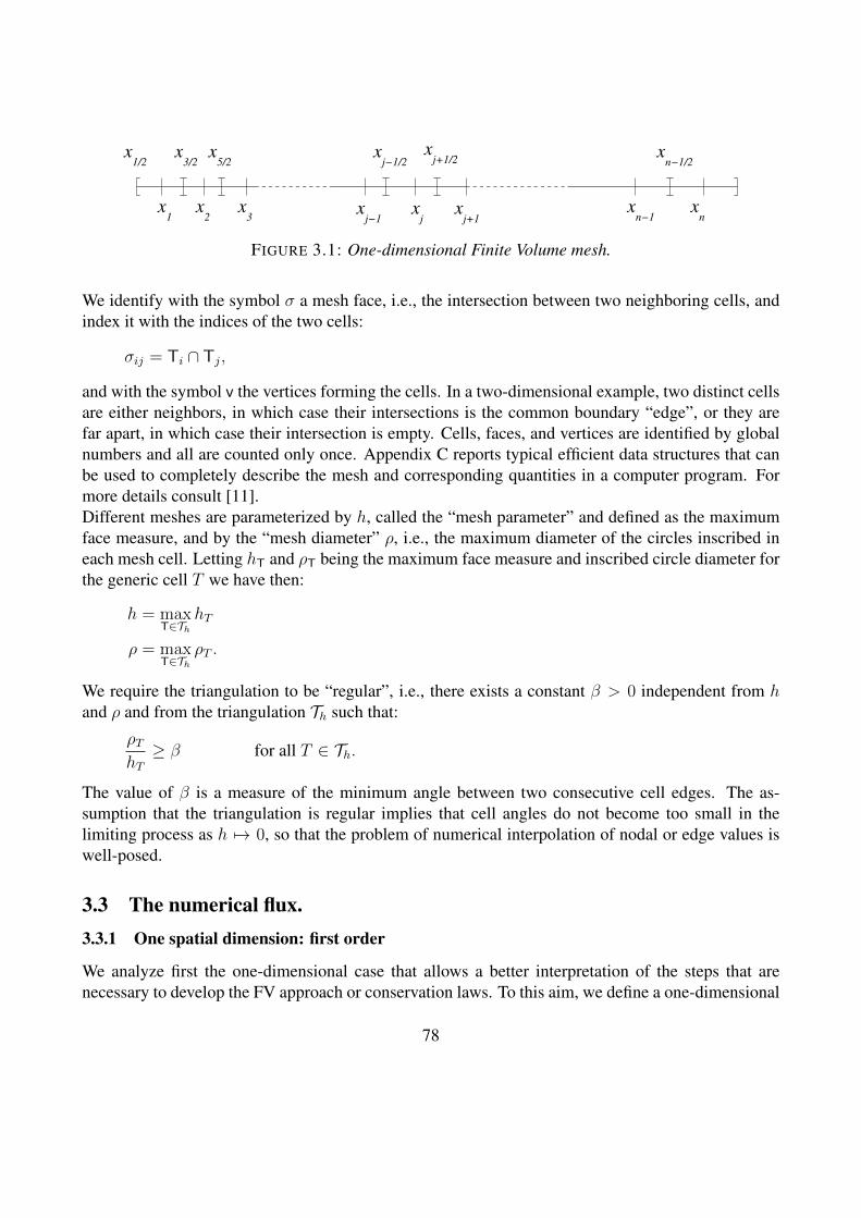
jx
1x
nx
n−1x
j−1x
j+1
xn−1/2
xj−1/2
x3/2
x5/2
x2
x3
xj+1/2
x1/2
x
FIGURE 3.1: One-dimensional Finite Volume mesh.
We identify with the symbol σ a mesh face, i.e., the intersection between two neighboring cells, andindex it with the indices of the two cells:
σij = Ti ∩ Tj,
and with the symbol v the vertices forming the cells. In a two-dimensional example, two distinct cellsare either neighbors, in which case their intersections is the common boundary “edge”, or they arefar apart, in which case their intersection is empty. Cells, faces, and vertices are identified by globalnumbers and all are counted only once. Appendix C reports typical efficient data structures that canbe used to completely describe the mesh and corresponding quantities in a computer program. Formore details consult [11].Different meshes are parameterized by h, called the “mesh parameter” and defined as the maximumface measure, and by the “mesh diameter” ρ, i.e., the maximum diameter of the circles inscribed ineach mesh cell. Letting hT and ρT being the maximum face measure and inscribed circle diameter forthe generic cell T we have then:
h = maxT∈Th
hT
ρ = maxT∈Th
ρT .
We require the triangulation to be “regular”, i.e., there exists a constant β > 0 independent from hand ρ and from the triangulation Th such that:
ρThT≥ β for all T ∈ Th.
The value of β is a measure of the minimum angle between two consecutive cell edges. The as-sumption that the triangulation is regular implies that cell angles do not become too small in thelimiting process as h 7→ 0, so that the problem of numerical interpolation of nodal or edge values iswell-posed.
3.3 The numerical flux.3.3.1 One spatial dimension: first order
We analyze first the one-dimensional case that allows a better interpretation of the steps that arenecessary to develop the FV approach or conservation laws. To this aim, we define a one-dimensional
78

grid as a non uniform subdivision of the domain into subintervals of dimension hi = dxi, where Tiis the i-th subdivision or Finite Volume cell. We denote by xi the center of the i-th cell and with x1+ 1
2
and x1− 12
its right and left boundary points (see Figure 3.1). We have the following relationships:
Ω = [a, b] =N⋃i=1
Ti =N⋃i=1
[x1− 1
2, x1+ 1
2
]; (3.10)
meas(Ω) =N∑i=1
(x1+ 1
2− x1− 1
2
)=
N∑i=1
dxi; (3.11)
Ti⋃
Ti+1 = x1+ 12. (3.12)
We want to discretize the one-dimensional conservation law:
ut + f(u)x = 0 x ∈ [a, b] and t ∈ [0, T ], (3.13)u(x, 0) = φ(x) t = 0. (3.14)
We redo the steps done in multidimension using now standard calculus. Integrate the equation inspace over the domain and in time over the subinterval [tk, tk+1] = ∆tk:∫ tk+1
tk
∫Ω (ut + f(u)x) dx dt = 0;
Using properties (3.10) and (3.12) together with the linearity of the integral operator we obtain:∫ tk+1
tk
∫ xj+1/2
xj−1/2
(ut + f(u)x) dx dt = 0, i = 1, . . . , N.
Define the cell average at time tk as:
ukh = Ah(u(tk)) =1
xj+1/2 − xj−1/2
∫ xj+1/2
xj−1/2
u(x, tk) dx =1
∆xk
∫ xj+1/2
xj−1/2
u(x, tk) dx,
and exchange the time derivative and the space integral in the first term to obtain after integration anduse of simple left evaluation of the temporal integral in the second term (Forward Euler):
uk+1h,i = ukh,i −
∆tk∆xi
[Gkh,i+1/2 − Gkh,i−1/2
]. (3.15)
We note that this equation is consistent with (3.9) as the outward unit normals in xj+1/2 and and xj−1/2
are 1 and -1, respectively.Now we need to evaluate the fluxes Gkh,i+1/2 and Gkh,i−1/2. These are obtained by solving a Riemannproblem at each cell interface ` = i − 1/2 and ` = i + 1/2, i.e., find the solution of equation (3.13)where the initial conditions are given by constant states uL and uR just on the left and on the rightof x`. Since we are using an explicit time-stepping scheme, the left and right conditions are thenumerical approximations of the cell averages at the previous time step ukh, and thus the Riemannproblem can be written as:
79
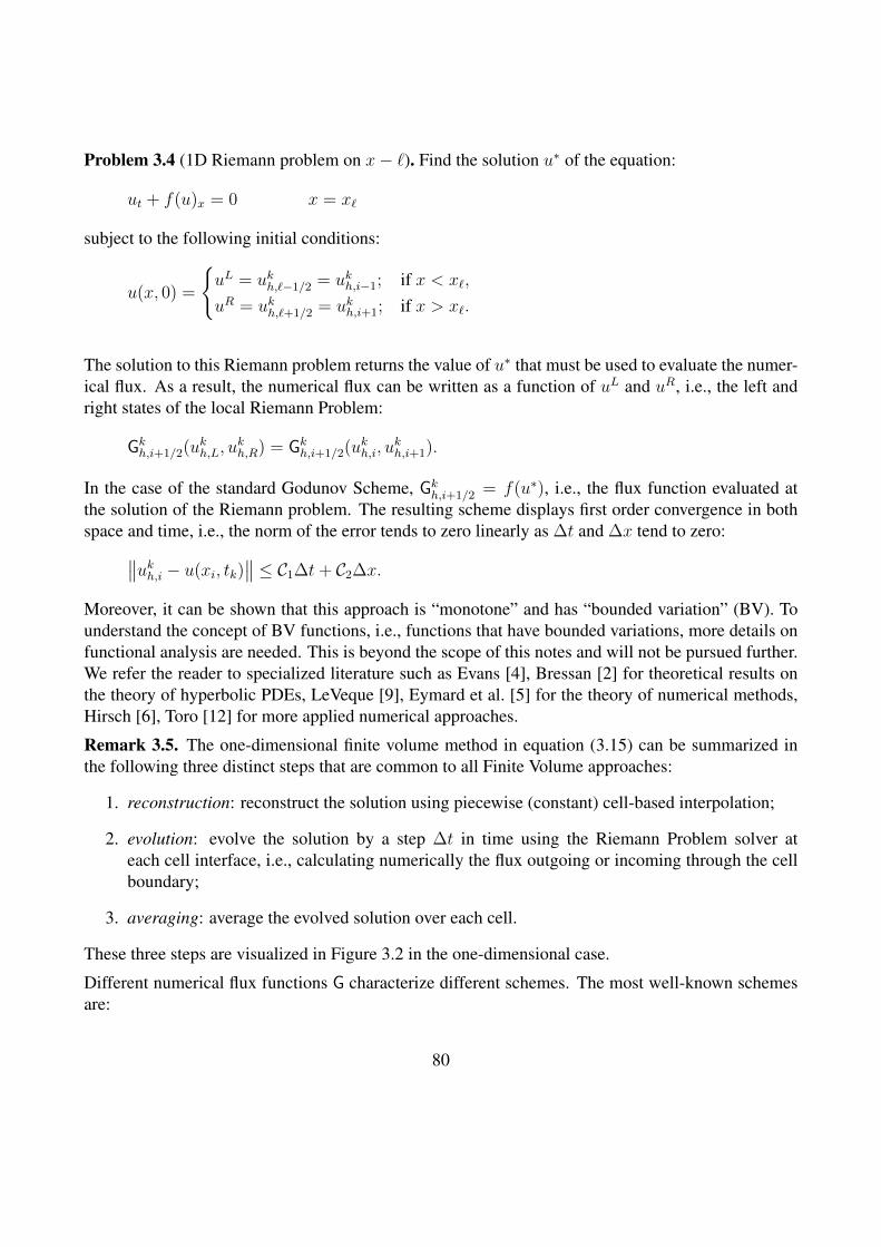
Problem 3.4 (1D Riemann problem on x− `). Find the solution u∗ of the equation:
ut + f(u)x = 0 x = x`
subject to the following initial conditions:
u(x, 0) =
uL = ukh,`−1/2 = ukh,i−1; if x < x`,
uR = ukh,`+1/2 = ukh,i+1; if x > x`.
The solution to this Riemann problem returns the value of u∗ that must be used to evaluate the numer-ical flux. As a result, the numerical flux can be written as a function of uL and uR, i.e., the left andright states of the local Riemann Problem:
Gkh,i+1/2(ukh,L, ukh,R) = Gkh,i+1/2(ukh,i, u
kh,i+1).
In the case of the standard Godunov Scheme, Gkh,i+1/2 = f(u∗), i.e., the flux function evaluated atthe solution of the Riemann problem. The resulting scheme displays first order convergence in bothspace and time, i.e., the norm of the error tends to zero linearly as ∆t and ∆x tend to zero:∥∥ukh,i − u(xi, tk)
∥∥ ≤ C1∆t+ C2∆x.
Moreover, it can be shown that this approach is “monotone” and has “bounded variation” (BV). Tounderstand the concept of BV functions, i.e., functions that have bounded variations, more details onfunctional analysis are needed. This is beyond the scope of this notes and will not be pursued further.We refer the reader to specialized literature such as Evans [4], Bressan [2] for theoretical results onthe theory of hyperbolic PDEs, LeVeque [9], Eymard et al. [5] for the theory of numerical methods,Hirsch [6], Toro [12] for more applied numerical approaches.
Remark 3.5. The one-dimensional finite volume method in equation (3.15) can be summarized inthe following three distinct steps that are common to all Finite Volume approaches:
1. reconstruction: reconstruct the solution using piecewise (constant) cell-based interpolation;
2. evolution: evolve the solution by a step ∆t in time using the Riemann Problem solver ateach cell interface, i.e., calculating numerically the flux outgoing or incoming through the cellboundary;
3. averaging: average the evolved solution over each cell.
These three steps are visualized in Figure 3.2 in the one-dimensional case.
Different numerical flux functions G characterize different schemes. The most well-known schemesare:
80

i− 52 i− 3
2 i− 12 i i+ 1
2 i+ 3/2i− 2 i− 1 i i+ 1 i+ 2
reconstruction
i− 52 i− 3
2 i− 12 i i + 1
2 i + 3/2i− 2 i− 1 i i + 1 i + 2
f ′(x)∆tevolution
i− 52 i− 3
2 i− 12 i i+ 1
2 i+ 3/2i− 2 i− 1 i i+ 1 i+ 2
averaging
FIGURE 3.2: The one-dimensional finite volume method subdivided in three steps: 1. reconstruction(top), 2. evolution (middle), 3. averaging (bottom).
Godunov
Gh,i+1/2(uh,i, uh,i+1) = f(u∗)
where u∗ is the solution of the local Riemann problem.
Lax-Friedrichs
Gh,i+1/2(uh,i, uh,i+1) =∆t
2∆x(uh,i − uh,i+1) +
1
2(f(uh,i) + f(uh,i+1))
Lax-Wendroff
Gkh,i+1/2 =f(uh,i) + f(uh,i+1)
2− ∆t
2∆xAi+1/2 (f(uh,i+1)− f(uh,i))
where A1+1/2 the Jacobian of f evaluated at xi+1/2. This Jacobian can be calculated eitheranalytically as f ′((uh,i + uh,i+1)/2) or numerically as
Ai+1/2 =
f(uh,i+1)−f(uh,iuh,i+1)−uh,i
if uh,i+1)− uh,i 6= 0
f(uh,i+1) otherwise.
The latter scheme is second order accurate in space and time while the first two schemes are only firstorder accurate.
Remark 3.6. We would like to stress here that Godunov method is the only scheme in the above listthat requires the solution of Riemann problems. The Lax-Friedrichs and Lax-Wendroff, in fact, do notrequire this step. These latter schemes are part of what is called the “central”, as opposed to “upwind”schemes, as described in ? ].
81

Example 3.7 (Riemann solver for Burger equation). For Burger equation we can define the followingexact Riemann solver:
1: procedure BURGER RS(uL, uR) .2: λ← f(uR)−f(uL)
uR−uL3: if uL > 0 AND uR > 0 then4: u∗ ← uL5: else if UL > 0 AND uR < 0 then6: if λ > 0 then7: u∗ ← uL8: else9: u∗ ← uR
10: end if11: else . Should be uL < 0 AND uL < uR12: u∗ ← 013: end if14: G← f(u∗) = 1
2(u∗)2
return G15: end procedure
Second order accuracy in time can be achieved by employing a higher order explicit time integrationsuch as the Runge method, a two-step Euler-based procedure. For Godunov scheme the following wehave the following:
uk+1/2h,i = ukh,i −
∆tk2∆xi
[Gkh,i+1/2 − Gkh,i−1/2
]uk+1h,i = ukh,i −
∆tk∆xi
[Gk+1/2h,i+1/2 − G
k+1/2h,i−1/2
].
Obtaining second order in space needs higher order (linear) interpolation of the cell based values, andthus the reconstruction of the solution gradient, to obtain second order accurate left and right statesfor the Riemann solution. This yields a spatially second order accurate evaluation of the numericalflux, leading to globally second order accurate schemes. We would like to remark here that secondorder accuracy can be achieved only away from the discontinuity, where only constant reconstruc-tion guarantees monotonicity. Thus, to avoid the introduction of oscillation, we need to develop anappropriate gradient reconstruction.
3.3.2 One spatial dimension: second order gradient reconstruction
Higher order of convergence of the spatial discretization is obtained in general by employing higherorder interpolation schemes. Second order interpolation is obtained by using linear polynomials toevaluate left and right states at cell interfaces. In this one-dimensional case, this can be obtained by
82
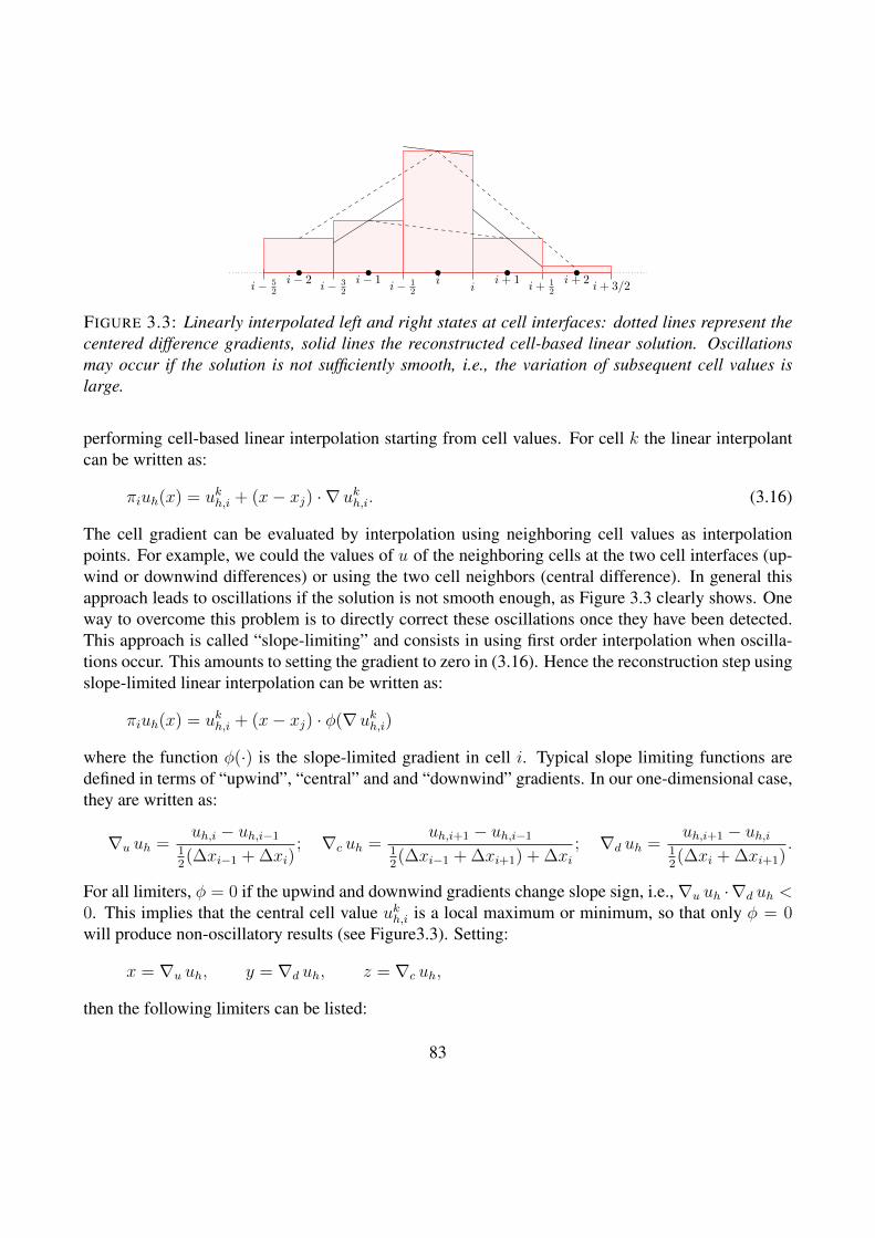
i− 52 i− 3
2 i− 12 i i+ 1
2 i+ 3/2i− 2 i− 1 i i+ 1 i+ 2
FIGURE 3.3: Linearly interpolated left and right states at cell interfaces: dotted lines represent thecentered difference gradients, solid lines the reconstructed cell-based linear solution. Oscillationsmay occur if the solution is not sufficiently smooth, i.e., the variation of subsequent cell values islarge.
performing cell-based linear interpolation starting from cell values. For cell k the linear interpolantcan be written as:
πiuh(x) = ukh,i + (x− xj) · ∇ukh,i. (3.16)
The cell gradient can be evaluated by interpolation using neighboring cell values as interpolationpoints. For example, we could the values of u of the neighboring cells at the two cell interfaces (up-wind or downwind differences) or using the two cell neighbors (central difference). In general thisapproach leads to oscillations if the solution is not smooth enough, as Figure 3.3 clearly shows. Oneway to overcome this problem is to directly correct these oscillations once they have been detected.This approach is called “slope-limiting” and consists in using first order interpolation when oscilla-tions occur. This amounts to setting the gradient to zero in (3.16). Hence the reconstruction step usingslope-limited linear interpolation can be written as:
πiuh(x) = ukh,i + (x− xj) · φ(∇ukh,i)
where the function φ(·) is the slope-limited gradient in cell i. Typical slope limiting functions aredefined in terms of “upwind”, “central” and and “downwind” gradients. In our one-dimensional case,they are written as:
∇u uh =uh,i − uh,i−1
12(∆xi−1 + ∆xi)
; ∇c uh =uh,i+1 − uh,i−1
12(∆xi−1 + ∆xi+1) + ∆xi
; ∇d uh =uh,i+1 − uh,i
12(∆xi + ∆xi+1)
.
For all limiters, φ = 0 if the upwind and downwind gradients change slope sign, i.e.,∇u uh ·∇d uh <0. This implies that the central cell value ukh,i is a local maximum or minimum, so that only φ = 0will produce non-oscillatory results (see Figure3.3). Setting:
x = ∇u uh, y = ∇d uh, z = ∇c uh,
then the following limiters can be listed:
83

MINMOD: (van Leer)
φ(x, y, z) = minmod(x, y) =
x if | x |<| y | and xy > 0;
y if | x |>| y | and xy > 0;
0 if xy ≤ 0.
MC - Monotonized Central Difference (van Leer):
φ(x, y, z) = minmod(2 minmod(x, y), z)
SUPERBEE (Roe):
φ(x, y, z) = maxmod(minmod(2x, y),minmod(x, 2y)),
where
maxmod(x, y) =
x if | x |>| y | and xy > 0;
y if | x |<| y | and xy > 0;
0 if xy ≤ 0.
Liu: 1. let:
uLi−1/2 = πi−1uh(xi−1/2); uRi+1/2 = πi+1uh(xi+1/2);
2. φ(x, y, z) = largest gradient among the three candidates x, y, z such that the reconstructededge values πiuh(xi−1/2) and πiuh(xi+1/2) satisfy:
uLi−1/2 ≤ πiuh(xi−1/2) ≤ uh,i and uh,i ≤ πiuh(xi+1/2) ≤ uRi+1/2,
84
A Finite Difference Approximations of first and second deriva-tives in R1.
The finite difference method (FD) is used to approximate derivatives of functions. We consider herethe derivation of the one dimensional standard approximations of the first and second derivativesof a function u(x) : I → R. To do so with simplicity we subdivide the interval I with a regularpartition with n subintervals of size ∆x, and indicate with the index j the nodes of the subdivision,j = 0, 1, . . . , n. The coordinates of the boundary of each subinterval are given by the coordinates oftwo successive nodes, xj and xj+1 = xj + ∆x. We denote by uh,j the numerical approximation ofthe solution at node xj: uh,j ≈ u(xk). Assuming u(x) sufficiently regular, we can write the followingTaylor expansions:
u(xj+1) = u(xj + ∆x) = u(xj) + ∆xux(xj) +∆x2
2uxx(xj) +O
(∆x3
)u(xj−1) = u(xj −∆x) = u(xj)−∆xux(xj) +
∆x2
2uxx(xj) +O
(∆x3
)The first derivative can be factored after subtracting the second equation from the first, to yield:
ux(xj) =u(xj+1)− u(xj−1)
2∆x+O
(∆x2
).
Then a second order “central” approximation to the first derivative is given by:
ux(xj) ≈uh,j+1 − uh,j−1
2∆x.
On the other hand, the first derivative can be obtained from the first or the second of the two Taylorseries expansions:
ux(xj) =u(xj+1)− u(xj)
∆x+O (∆x) ,
ux(xj) =u(xj)− u(xj−1)
∆x+O (∆x) ,
yielding forward or backward first order approximations:
ux(xj) ≈uh,j+1 − uh,j
∆x,
ux(xj) ≈uh,j − uh,j−1
∆x.
85
Summing the two Taylor series expressions, we obtain a second order approximation of the secondderivative:
uxx(xj) =u(xj+1)− 2u(xj) + u(xj−1)
∆x2+O
(∆x2
),
uxx(xj) ≈uh,j+1 − 2uh,j + uh,j−1
∆x2.
86
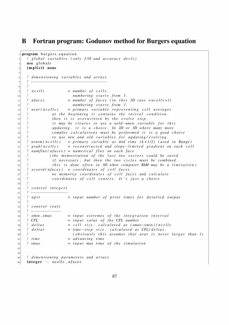
B Fortran program: Godunov method for Burgers equation
1 program b u r g e r s e q u a t i o n2 ! g l o b a l v a r i a b l e s ( o n l y I /O and a c c u r a c y d e c l s )3 use g l o b a l s4 i m p l i c i t none5
6 ! d i m e n s i o n i n g v a r i a b l e s and a r r a y s7 ! −−−−−−−−−−−−−−−−−−−−−−−−−−−−−−−−−8 !9 ! n c e l l s = number o f c e l l s .
10 ! numbering s t a r t s from 1 .11 ! n f a c e s = number o f f a c e s ( i n t h i s 1D case = n c e l l s +1)12 ! numbering s t a r t s from 1 .13 ! uvar ( n c e l l s ) = pr imary v a r i a b l e r e p r e s e n t i n g c e l l a v e r a g e s14 ! a t t h e b e g i n n i n g i t c o n t a i n s t h e i n i t i a l c o n d i t i o n .15 ! t h e n i t i s o v e r w r i t t e n by t h e e v o l v e s t e p .16 ! i t may be c l e a r e r t o use a uold−unew v a r i a b l e f o r t h i s17 ! u p d a t i n g . i t i s a c h o i c e . In 2D or 3D where many more18 ! complex c a l c u l a t i o n s must be per fo rmed i t i s a good c h o i c e19 ! t o use new and o l d v a r i a b l e s f o r u p d a t i n g / e v o l v i n g .20 ! uvarm ( n c e l l s ) = pr imary v a r i a b l e a t mid t i m e ( k +1/2 ) ( used i n Runge )21 ! grad ( n c e l l s ) = r e c o n s t r u c t e d and s l o p e− l i m i t e d g r a d i e n t on each c e l l22 ! numf lux ( n f a c e s ) = n u m e r i c a l f l u x on each f a c e23 ! ( t h e m e m o r i z a t i o n o f t h e l a s t two v e c t o r s c o u l d be saved24 ! i f n e c e s s a r y , b u t t h e n t h e two c y c l e s must be combined .25 ! t h i s i s done o f t e n i n 3D when computer RAM may be a l i m i t a t i o n )26 ! xcoord ( n f a c e s ) = c o o r d i n a t e s o f c e l l f a c e s27 ! we memorize c o o r d i n a t e s o f c e l l f a c e s and c a l c u l a t e28 ! c o o r d i n a t e s o f c e l l c e n t e r s . I t ’ s j u s t a c h o i c e29 !30 ! c o n t r o l i n t e g e r s31 ! −−−−−−−−−−−−−−−−32 ! n p r t = i n p u t number o f p r i n t t i m e s f o r d e t a i l e d o u t p u t33 !34 ! c o n t r o l r e a l s35 ! −−−−−−−−−−−−−36 ! xmin , xmax = i n p u t e x t r e m e s o f t h e i n t e g r a t i o n i n t e r v a l37 ! CFL = i n p u t v a l u e o f t h e CFL number38 ! d e l t a x = c e l l s i z e . c a l c u l a t e d as ( xmax−xmin ) / n c e l l s39 ! d e l t a t = t ime−s t e p s i z e . c a l c u l a t e d as CFL / d e l t a x .40 ! ( o b v i o u s l y t h i s assumes t h a t uvar i s n e v e r l a r g a r than 1)41 ! t i m e = advanc ing t i m e42 ! tmax = i n p u t max t i m e o f t h e s i m u l a t i o n43
44
45 ! d i m e n s i o n i n g p a r a m e t e r s and a r r a y s46 i n t e g e r : : n c e l l s , n f a c e s
87

47 r e a l ( kind=double ) , a l l o c a t a b l e : : uva r ( : ) , g r ad ( : ) , uvarm ( : )48 r e a l ( kind=double ) , a l l o c a t a b l e : : numflux ( : ) , xcoord ( : )49
50 ! c o n t r o l i n t e g e r s51 i n t e g e r : : n p r t , t s t y p e , l i m i t e r52
53 ! c o n t r o l r e a l s54 r e a l ( kind=double ) : : xmin , xmax55 r e a l ( kind=double ) : : CFL , d e l t a t , d e l t a x56 r e a l ( kind=double ) : : t ime , tmax57
58 ! l o c a l i n t e g e r s59 i n t e g e r : : i t i m e , p r t t i m e60
61 c a l l r e a d d a t a ( n c e l l s , n f a c e s , n p r t , t s t y p e , l i m i t e r , xmin , xmax , CFL , tmax )62
63 a l l o c a t e ( xcoord ( 1 : n f a c e s ) )64 a l l o c a t e ( uva r ( 1 : n c e l l s ) )65 a l l o c a t e ( uvarm ( 1 : n c e l l s ) )66 a l l o c a t e ( g r ad ( 1 : n c e l l s ) )67 a l l o c a t e ( numflux ( 1 : n f a c e s ) )68
69 c a l l i n i t ( n c e l l s , n f a c e s , xmin , xmax , CFL , d e l t a x , d e l t a t , xcoord , uvarm )70
71 c a l l d e t o u t p u t ( n c e l l s , n f a c e s , t ime , xcoord , uvarm )72 c a l l dcopy ( n c e l l s , uvarm , 1 , uvar , 1 )73
74 p r t t i m e =max ( ( i n t ( tmax / d e l t a t ) + 1 ) / n p r t , 1 )75 i t i m e =076
77 t ime = 0 . 078 do whi l e ( t ime . l t . tmax )79
80 i f ( t s t y p e . eq . 1 ) then ! i f Runge81 c a l l Godunov 2nd orde r ( n c e l l s , n f a c e s , l i m i t e r , CFL / 2 , xcoord , grad , numflux ,
uvar , uvarm )82 end i f83 c a l l Godunov 2nd orde r ( n c e l l s , n f a c e s , l i m i t e r , CFL , xcoord , grad , numflux , uvar ,
uvarm )84
85 ! u p d a t e s new s o l u t i o n f o r n e x t t i m e s t e p86 !87 c a l l dcopy ( n c e l l s , uvarm , 1 , uvar , 1 )88
89 i f ( t ime + d e l t a t . gt . tmax ) d e l t a t = tmax−t ime90 t ime = t ime + d e l t a t91 i t i m e = i t i m e +192
93 i f (mod ( i t i m e , p r t t i m e ) . eq . 0 ) &
88
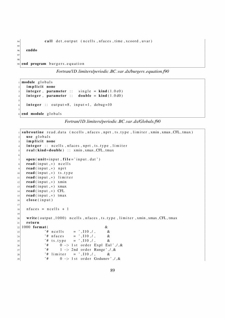
94 c a l l d e t o u t p u t ( n c e l l s , n f a c e s , t ime , xcoord , uva r )95
96 enddo97
98
99 end program b u r g e r s e q u a t i o n
Fortran/1D limiters/periodic BC var dx/burgers equation.f90
1 module g l o b a l s2 i m p l i c i t none3 i n t e g e r , parameter : : s i n g l e = kind ( 1 . 0 e0 )4 i n t e g e r , parameter : : double = kind ( 1 . 0 d0 )5
6 i n t e g e r : : o u t p u t =8 , i n p u t =1 , debug =107
8 end module g l o b a l s
Fortran/1D limiters/periodic BC var dx/Globals.f90
1 s u b r o u t i n e r e a d d a t a ( n c e l l s , n f a c e s , n p r t , t s t y p e , l i m i t e r , xmin , xmax , CFL , tmax )2 use g l o b a l s3 i m p l i c i t none4 i n t e g e r : : n c e l l s , n f a c e s , n p r t , t s t y p e , l i m i t e r5 r e a l ( kind=double ) : : xmin , xmax , CFL , tmax6
7 open ( u n i t = i n p u t , f i l e = ’ i n p u t . d a t ’ )8 read ( i n p u t , ∗ ) n c e l l s9 read ( i n p u t , ∗ ) n p r t
10 read ( i n p u t , ∗ ) t s t y p e11 read ( i n p u t , ∗ ) l i m i t e r12 read ( i n p u t , ∗ ) xmin13 read ( i n p u t , ∗ ) xmax14 read ( i n p u t , ∗ ) CFL15 read ( i n p u t , ∗ ) tmax16 c l o s e ( i n p u t )17
18 n f a c e s = n c e l l s + 119
20 w r i t e ( o u t p u t , 1 0 0 0 ) n c e l l s , n f a c e s , t s t y p e , l i m i t e r , xmin , xmax , CFL , tmax21 re turn22 1000 format ( &23 ’ # n c e l l s = ’ , I10 , / , &24 ’ # n f a c e s = ’ , I10 , / , &25 ’ # t s t y p e = ’ , I10 , / , &26 ’ # 0 −> 1 s t o r d e r Expl Eul ’ , / ,&27 ’ # 1 −> 2nd o r d e r Runge ’ , / ,&28 ’ # l i m i t e r = ’ , I10 , / , &29 ’ # 0 −> 1 s t o r d e r Godunov ’ , / ,&
89

30 ’ # 1 −> 2nd o r d e r minmod ’ , / ,&31 ’ # 2 −> 2nd o r d e r MC’ , / ,&32 ’ # 3 −> 2nd o r d e r s u p e r b e e ’ , / ,&33 ’ # 4 −> 2nd o r d e r Liu ’ , / ,&34 ’ # xmin = ’ ,1 pe12 . 4 , / , &35 ’ # xmax = ’ ,1 pe12 . 4 , / , &36 ’ # CFL = ’ ,1 pe12 . 4 , / , &37 ’ # Tmax = ’ ,1 pe12 . 4 )38 end s u b r o u t i n e r e a d d a t a
Fortran/1D limiters/periodic BC var dx/read data.f90
1 s u b r o u t i n e i n i t ( n c e l l s , n f a c e s , xmin , xmax , CFL , d e l t a x , d e l t a t , &2 xcoord , uo ld )3 use g l o b a l s4 i m p l i c i t none5 i n t e g e r : : n c e l l s , n f a c e s6 r e a l ( kind=double ) : : xcoord ( n f a c e s ) , uo ld ( n c e l l s )7 r e a l ( kind=double ) : : xmin , xmax , CFL , d e l t a x , d e l t a t8
9 r e a l ( kind=double ) , parameter : : z e r o =0 .0 d0 , one =1 .0 d0 , t h r e e =3 .0 d0 , a h a l f =0 .5 d010 r e a l ( kind=double ) , parameter : : p i =4 .0 d0∗ atan ( 1 . 0 d0 )11
12 i n t e g e r : : i13
14 ! he re I am u s i n g u n i f o r m s p a c i n g b u t i t ’ s coded so t h a t15 ! i t can be non u n i f o r m by chang ing t h e n e x t l i n e s16 ! xcoord are t h e f a c e ( node ) c o o r d i n a t e s , t h e c e l l c e n t e r s17 ! are s h i f t e d by d e l t a x / 2 t o t h e r i g h t w i t h r e s p e c t t o xcoord18 ! I amalso assuming t h e i n i t i a l c o n d i t i o n i s n o t l a r g e r than 119 !20 d e l t a x =( xmax−xmin ) / n c e l l s21 d e l t a t = d e l t a x ∗CFL22
23 do i =1 , n f a c e s24 xcoord ( i ) =xmin + ( i −1) ∗ d e l t a x25 enddo26 !27 ! i n i t i a l c o n d i t i o n s28 ! i n i t i a l u must be c o n s i s t e n t w i t h BCs ( i f p r e s e n t )29 !30 do i =1 , n c e l l s31 ! uo ld ( i ) = one / ( one + ( xcoord ( i ) + d e l t a x ∗ a h a l f − t h r e e ) ∗∗2)32 uo ld ( i ) = s i n (2∗ p i ∗ ( xcoord ( i ) ) )33 end do34 ! do i =1 , n c e l l s35 ! uo ld ( i ) = z e r o36 ! end do37 ! uo ld ( 1 ) = one
90

38
39 end s u b r o u t i n e i n i t
Fortran/1D limiters/periodic BC var dx/init.f90
1 s u b r o u t i n e d e t o u t p u t ( n c e l l s , n f a c e s , t ime , xcoord , u )2 use g l o b a l s3 i m p l i c i t none4
5 i n t e g e r : : n c e l l s , n f a c e s6 r e a l ( kind=double ) , dimension ( n c e l l s ) : : u7 r e a l ( kind=double ) , dimension ( n f a c e s ) : : xcoord8 r e a l ( kind=double ) : : t ime , d e l t a x9
10 r e a l ( kind=double ) : : a h a l f =0 .5 d011
12 i n t e g e r : : i13
14 w r i t e ( o u t p u t , ’ ( a , e15 . 5 ) ’ ) ’ # t ime = ’ , t ime15 do i =1 , n c e l l s16 d e l t a x = ( xcoord ( i +1)−xcoord ( i ) )17 w r i t e ( o u t p u t , ’ (2 e15 . 5 ) ’ ) ( xcoord ( i ) + xcoord ( i +1) ) ∗ a h a l f , u ( i )18 end do19
20 end s u b r o u t i n e d e t o u t p u t
Fortran/1D limiters/periodic BC var dx/det output.f90
1 s u b r o u t i n e Godunov 2nd orde r ( n c e l l s , n f a c e s , l i m i t e r , CFL , xcoord , grad , numflux , uvar, uvarm )
2 use g l o b a l s3 i m p l i c i t none4
5 ! exchange v a r i a b l e s6 i n t e g e r : : n c e l l s , n f a c e s , l i m i t e r7 r e a l ( kind=double ) : : CFL8 r e a l ( kind=double ) : : xcoord ( n f a c e s ) , g r ad ( n c e l l s ) , uva r ( n c e l l s ) , uvarm ( n c e l l s )9 r e a l ( kind=double ) : : numflux ( n f a c e s )
10
11 ! he re we work on c e l l s12 c a l l g r a d r e c o n s t r u c t i o n ( n f a c e s , n c e l l s , l i m i t e r , xcoord , uvarm , g rad )13
14 ! he re we work on f a c e s15 c a l l r i e m a n s o l v e ( n f a c e s , n c e l l s , xcoord , grad , uvarm , numflux )16
17 ! he re we work on c e l l s18 c a l l e v o l v e ( n c e l l s , n f a c e s , CFL , uvar , uvarm , numflux )19
20 end s u b r o u t i n e Godunov 2nd orde r
91

Fortran/1D limiters/periodic BC var dx/godunov 2nd order.f90
1 s u b r o u t i n e g r a d r e c o n s t r u c t i o n ( n f a c e s , n c e l l s , l i m i t e r , xcoord , uvar , g r ad )2 use g l o b a l s3 i m p l i c i t none4
5 ! exchange v a r i a b l e s6 i n t e g e r : : n f a c e s , n c e l l s , l i m i t e r7 r e a l ( kind=double ) : : d e l t a x c e l l , d e l t a x u p w i n d , de l tax dwnwnd8 r e a l ( kind=double ) : : xcoord ( n f a c e s ) , uva r ( n c e l l s ) , g r ad ( n c e l l s )9
10 ! e x t e r n a l f u n c t i o n s11 r e a l ( kind=double ) : : s l o p e l i m i t12
13 ! l o c a l v a r i a b l e s14 i n t e g e r : : i c e l l , index upwind , i n d e x c e l l , index dwnwnd15 r e a l ( kind=double ) : : u upwind , u c e l l , u dwnwnd16 r e a l ( kind=double ) : : g r a d c a n d i d a t e ( 3 )17
18 ! l o c a l p a r a m e t e r s19 r e a l ( kind=double ) : : a h a l f =0 .5 d020
21 ! r e c o n s t r u c t i o n i s done on c e l l s22 ! need t o check f o r boundary on f a c e s ( he re u s i n g p e r i o d i c BCs )23 do i c e l l =1 , n c e l l s24
25 i ndex upwind = i c e l l − 126 i n d e x c e l l = i c e l l27 index dwnwnd = i c e l l + 128 i f ( i ndex upwind . l e . 0 ) then29 ! on t h e l e f t boundary : t h e v a l u e o f t h e upwind c e l l i s t a k e n30 ! from t h e l a s t c e l l31 i ndex upwind = n c e l l s32 end i f33 i f ( index dwnwnd . ge . n c e l l s ) then34 ! on t h e r i g h t boundary : t h e v a l u e o f t h e downwind c e l l i s t a k e n35 ! from t h e f i r s t c e l l36 index dwnwnd = 137 end i f38 d e l t a x u p w i n d = xcoord ( index upwind +1)−xcoord ( index upwind )39 del tax dwnwnd = xcoord ( index dwnwnd +1)−xcoord ( index dwnwnd )40 d e l t a x c e l l = xcoord ( i n d e x c e l l +1)−xcoord ( i n d e x c e l l )41
42 u upwind = uva r ( i ndex upwind )43 u c e l l = uva r ( i n d e x c e l l )44 u dwnwnd = uva r ( index dwnwnd )45
46 g r a d c a n d i d a t e ( 1 ) = ( u c e l l − u upwind ) / ( a h a l f ∗ ( d e l t a x c e l l + d e l t a x u p w i n d ) )
92
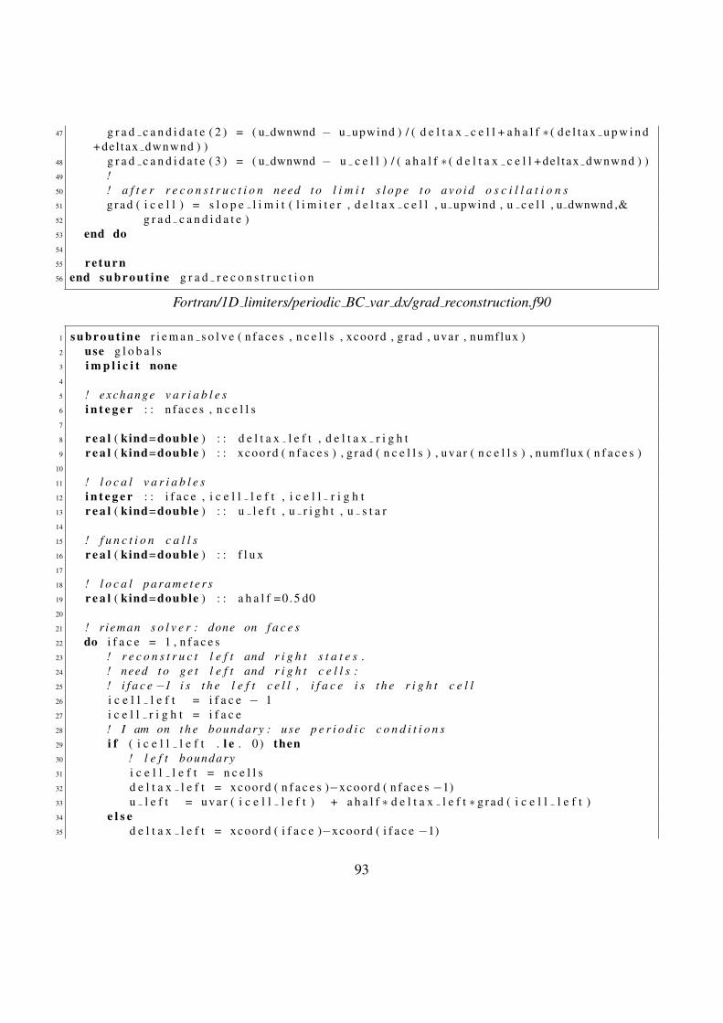
47 g r a d c a n d i d a t e ( 2 ) = ( u dwnwnd − u upwind ) / ( d e l t a x c e l l + a h a l f ∗ ( d e l t a x u p w i n d+ del tax dwnwnd ) )
48 g r a d c a n d i d a t e ( 3 ) = ( u dwnwnd − u c e l l ) / ( a h a l f ∗ ( d e l t a x c e l l + de l tax dwnwnd ) )49 !50 ! a f t e r r e c o n s t r u c t i o n need t o l i m i t s l o p e t o a v o i d o s c i l l a t i o n s51 g rad ( i c e l l ) = s l o p e l i m i t ( l i m i t e r , d e l t a x c e l l , u upwind , u c e l l , u dwnwnd ,&52 g r a d c a n d i d a t e )53 end do54
55 re turn56 end s u b r o u t i n e g r a d r e c o n s t r u c t i o n
Fortran/1D limiters/periodic BC var dx/grad reconstruction.f90
1 s u b r o u t i n e r i e m a n s o l v e ( n f a c e s , n c e l l s , xcoord , grad , uvar , numflux )2 use g l o b a l s3 i m p l i c i t none4
5 ! exchange v a r i a b l e s6 i n t e g e r : : n f a c e s , n c e l l s7
8 r e a l ( kind=double ) : : d e l t a x l e f t , d e l t a x r i g h t9 r e a l ( kind=double ) : : xcoord ( n f a c e s ) , g r ad ( n c e l l s ) , uva r ( n c e l l s ) , numflux ( n f a c e s )
10
11 ! l o c a l v a r i a b l e s12 i n t e g e r : : i f a c e , i c e l l l e f t , i c e l l r i g h t13 r e a l ( kind=double ) : : u l e f t , u r i g h t , u s t a r14
15 ! f u n c t i o n c a l l s16 r e a l ( kind=double ) : : f l u x17
18 ! l o c a l p a r a m e t e r s19 r e a l ( kind=double ) : : a h a l f =0 .5 d020
21 ! r ieman s o l v e r : done on f a c e s22 do i f a c e = 1 , n f a c e s23 ! r e c o n s t r u c t l e f t and r i g h t s t a t e s .24 ! need t o g e t l e f t and r i g h t c e l l s :25 ! i f a c e −1 i s t h e l e f t c e l l , i f a c e i s t h e r i g h t c e l l26 i c e l l l e f t = i f a c e − 127 i c e l l r i g h t = i f a c e28 ! I am on t h e boundary : use p e r i o d i c c o n d i t i o n s29 i f ( i c e l l l e f t . l e . 0 ) then30 ! l e f t boundary31 i c e l l l e f t = n c e l l s32 d e l t a x l e f t = xcoord ( n f a c e s )−xcoord ( n f a c e s −1)33 u l e f t = uva r ( i c e l l l e f t ) + a h a l f ∗ d e l t a x l e f t ∗ g rad ( i c e l l l e f t )34 e l s e35 d e l t a x l e f t = xcoord ( i f a c e )−xcoord ( i f a c e −1)
93
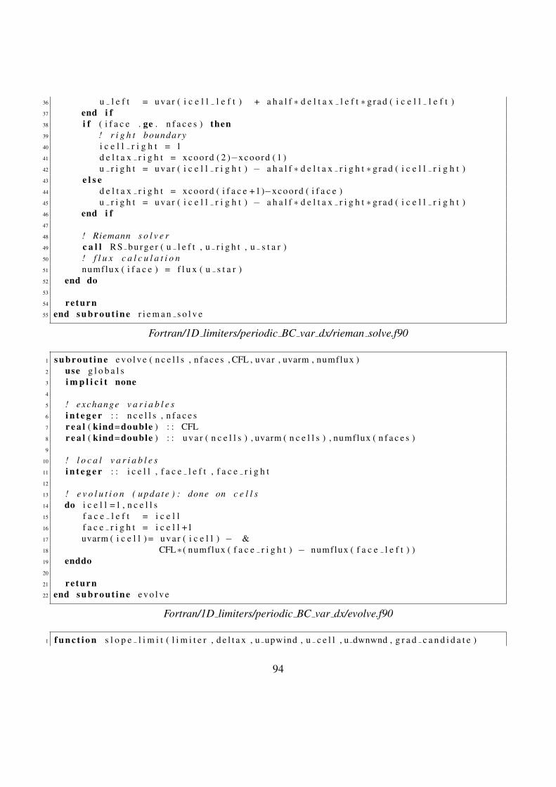
36 u l e f t = uva r ( i c e l l l e f t ) + a h a l f ∗ d e l t a x l e f t ∗ g rad ( i c e l l l e f t )37 end i f38 i f ( i f a c e . ge . n f a c e s ) then39 ! r i g h t boundary40 i c e l l r i g h t = 141 d e l t a x r i g h t = xcoord ( 2 )−xcoord ( 1 )42 u r i g h t = uva r ( i c e l l r i g h t ) − a h a l f ∗ d e l t a x r i g h t ∗ g rad ( i c e l l r i g h t )43 e l s e44 d e l t a x r i g h t = xcoord ( i f a c e +1)−xcoord ( i f a c e )45 u r i g h t = uva r ( i c e l l r i g h t ) − a h a l f ∗ d e l t a x r i g h t ∗ g rad ( i c e l l r i g h t )46 end i f47
48 ! Riemann s o l v e r49 c a l l RS burge r ( u l e f t , u r i g h t , u s t a r )50 ! f l u x c a l c u l a t i o n51 numflux ( i f a c e ) = f l u x ( u s t a r )52 end do53
54 re turn55 end s u b r o u t i n e r i e m a n s o l v e
Fortran/1D limiters/periodic BC var dx/rieman solve.f90
1 s u b r o u t i n e e v o l v e ( n c e l l s , n f a c e s , CFL , uvar , uvarm , numflux )2 use g l o b a l s3 i m p l i c i t none4
5 ! exchange v a r i a b l e s6 i n t e g e r : : n c e l l s , n f a c e s7 r e a l ( kind=double ) : : CFL8 r e a l ( kind=double ) : : uva r ( n c e l l s ) , uvarm ( n c e l l s ) , numflux ( n f a c e s )9
10 ! l o c a l v a r i a b l e s11 i n t e g e r : : i c e l l , f a c e l e f t , f a c e r i g h t12
13 ! e v o l u t i o n ( u pda t e ) : done on c e l l s14 do i c e l l =1 , n c e l l s15 f a c e l e f t = i c e l l16 f a c e r i g h t = i c e l l +117 uvarm ( i c e l l ) = uva r ( i c e l l ) − &18 CFL∗ ( numflux ( f a c e r i g h t ) − numflux ( f a c e l e f t ) )19 enddo20
21 re turn22 end s u b r o u t i n e e v o l v e
Fortran/1D limiters/periodic BC var dx/evolve.f90
1 f u n c t i o n s l o p e l i m i t ( l i m i t e r , d e l t a x , u upwind , u c e l l , u dwnwnd , g r a d c a n d i d a t e )
94

2 use g l o b a l s3 i m p l i c i t none4
5 ! exchange v a r i a b l e s6 i n t e g e r : : l i m i t e r7
8 r e a l ( kind=double ) : : d e l t a x9 r e a l ( kind=double ) : : u upwind , u c e l l , u dwnwnd
10 r e a l ( kind=double ) : : g r a d c a n d i d a t e ( 3 )11
12 r e a l ( kind=double ) : : s l o p e l i m i t13
14 ! e x t e r n a l f u n c t i o n s15 r e a l ( kind=double ) : : minmod , maxmod , Liu16
17 ! l o c a l v a r i a b l e s18 r e a l ( kind=double ) : : g rad upwind , grad dwnwnd , g r a d c e n t e r , s l ope1 , s l o p e 219 ! l o c a l p a r a m e t e r s20 r e a l ( kind=double ) : : z e r o =0 .0 d0 , two =2 .0 d021
22 grad upwind = g r a d c a n d i d a t e ( 1 )23 g r a d c e n t e r = g r a d c a n d i d a t e ( 2 )24 grad dwnwnd = g r a d c a n d i d a t e ( 3 )25 s e l e c t case ( l i m i t e r )26 case ( 1 ) ! minmod27 s l o p e l i m i t = minmod ( grad upwind , grad dwnwnd )28
29 case ( 2 ) ! MC30 s l o p e l i m i t = minmod ( two∗minmod ( grad upwind , grad dwnwnd ) , &31 g r a d c e n t e r )32
33 case ( 3 ) ! s u p e r b e e34 s l o p e 1 = minmod ( grad dwnwnd , two∗ grad upwind )35 s l o p e 2 = minmod ( two∗grad dwnwnd , g rad upwind )36 s l o p e l i m i t = maxmod ( s lope1 , s l o p e 2 )37
38 case ( 4 ) ! L iu39 s l o p e l i m i t = Liu ( d e l t a x , u c e l l , u upwind , u dwnwnd , g r a d c a n d i d a t e )40
41 case d e f a u l t ! godunov 1 s t o r d e r42 s l o p e l i m i t = z e r o43 end s e l e c t44
45 end f u n c t i o n s l o p e l i m i t
Fortran/1D limiters/periodic BC var dx/slope limit.f90
1 f u n c t i o n Liu ( d e l t a x , u c e l l , u upwind , u dwnwnd , g r a d c a n d i d a t e )2 use g l o b a l s
95

3 i m p l i c i t none4
5 ! exchange v a r i a b l e s6
7 r e a l ( kind=double ) : : d e l t a x , u c e l l , u upwind , u dwnwnd8 r e a l ( kind=double ) : : Liu9 r e a l ( kind=double ) : : g r a d c a n d i d a t e ( 3 )
10
11 ! l o c a l v a r i a b l e s12
13 r e a l ( kind=double ) : : g rad upwind , grad dwnwnd14 r e a l ( kind=double ) : : l e f t p r o d , r i g h t p r o d , u l e f t , u r i g h t15 r e a l ( kind=double ) : : z e r o =0 .0 d0 , a h a l f =0 .5 d016
17 i n t e g e r : : i n d ( 3 )18 i n t e g e r : : i g r a d19
20 c a l l s o r t 3 ( g r a d c a n d i d a t e , i n d )21 grad upwind = g r a d c a n d i d a t e ( 1 )22 grad dwnwnd= g r a d c a n d i d a t e ( 3 )23
24 i f ( g rad upwind ∗grad dwnwnd . l t . z e r o ) then25 !26 ! i n t h i s case t h e c e n t r a l c e l l i s a t a max27 Liu = z e r o28 e l s e29 Liu = z e r o30 !31 ! i n t h i s case one o f t h e g r a d i e n t i s c e r t a i n l y ok32 ! r e c o n s t r u c t f a c e v a l u e on t h e l e f t and on t h e r i g h t33 do i g r a d =1 ,334 u l e f t = u c e l l − a h a l f ∗ d e l t a x ∗ g r a d c a n d i d a t e ( i n d ( i g r a d ) )35 u r i g h t = u c e l l + a h a l f ∗ d e l t a x ∗ g r a d c a n d i d a t e ( i n d ( i g r a d ) )36 !37 ! l e f t ( r i g h t ) p ro d i s >=0 i f u upwind<=u l e f t <=u c e l l or v i c e v e r s a38 l e f t p r o d = ( u upwind−u l e f t ) ∗ ( u l e f t −u c e l l )39 r i g h t p r o d = ( u c e l l −u r i g h t ) ∗ ( u r i g h t −u dwnwnd )40
41 i f ( l e f t p r o d ∗ r i g h t p r o d . ge . z e r o ) then42 Liu = g r a d c a n d i d a t e ( i n d ( i g r a d ) )43 re turn44 end i f45 end do46 end i f47
48 end f u n c t i o n Liu49
50 f u n c t i o n minmod ( a , b )51 use g l o b a l s
96

52 i m p l i c i t none53
54 r e a l ( kind=double ) : : a , b55 r e a l ( kind=double ) : : minmod56
57 r e a l ( kind=double ) : : z e r o =0 .0 d058
59 i f ( a∗b . l t . z e r o ) then60 minmod = z e r o61 e l s e i f ( abs ( a ) . l t . abs ( b ) ) then62 minmod = a63 e l s e64 minmod = b65 e n d i f66
67 end f u n c t i o n minmod68
69 f u n c t i o n maxmod ( a , b )70 use g l o b a l s71 i m p l i c i t none72
73 r e a l ( kind=double ) : : a , b74 r e a l ( kind=double ) : : maxmod75
76 r e a l ( kind=double ) : : z e r o =0 .0 d077
78 i f ( a∗b . l t . z e r o ) then79 maxmod = z e r o80 e l s e i f ( abs ( a ) . gt . abs ( b ) ) then81 maxmod = a82 e l s e83 maxmod = b84 e n d i f85
86 end f u n c t i o n maxmod
Fortran/1D limiters/periodic BC var dx/limiters.f90
1 s u b r o u t i n e RS burge r ( u l e f t , u r i g h t , u s t a r )2 use g l o b a l s3 i m p l i c i t none4
5 ! exchange v a r i a b l e s6 r e a l ( kind=double ) : : u l e f t , u r i g h t , u s t a r7
8 ! l o c a l f u n c t i o n s c a l l e d9 r e a l ( kind=double ) : : f l u x , j a c
10
11 ! l o c a l v a r i a b l e s
97

12 r e a l ( kind=double ) : : j a c l e f t , j a c r i g h t , f l e f t , f r i g h t , lambda13
14 ! l o c a l p a r a m e t e r s15 r e a l ( kind=double ) : : z e r o =0 .0 d016
17 j a c l e f t = j a c ( u l e f t )18 j a c r i g h t = j a c ( u r i g h t )19 f l e f t = f l u x ( u l e f t )20 f r i g h t = f l u x ( u r i g h t )21
22 lambda = ( f l e f t − f r i g h t ) / ( u l e f t −u r i g h t )23
24 ! c a s e s25 i f ( j a c l e f t . ge . z e r o . and . j a c r i g h t . ge . z e r o ) then26 ! case 1 .27 u s t a r = u l e f t28 e l s e i f ( j a c l e f t . l e . z e r o . and . j a c r i g h t . l e . z e r o ) then29 u s t a r = u r i g h t30 e l s e i f ( j a c l e f t . ge . z e r o . and . j a c l e f t . ge . j a c r i g h t ) then31 i f ( lambda . gt . z e r o ) then32 u s t a r = u l e f t33 e l s e34 u s t a r = u r i g h t35 end i f36 e l s e i f ( j a c l e f t . l t . z e r o . and . j a c l e f t . l t . j a c r i g h t ) then37 u s t a r = z e r o38 end i f39
40 re turn41 end s u b r o u t i n e RS burge r
Fortran/1D limiters/periodic BC var dx/RS burger.f90
1 f u n c t i o n f l u x ( u )2 use g l o b a l s3 i m p l i c i t none4
5 r e a l ( kind=double ) : : f l u x , u6
7 r e a l ( kind=double ) : : a h a l f =0 .5 d08
9 f l u x = a h a l f ∗ u∗∗210
11 re turn12 end f u n c t i o n f l u x13
14
15 f u n c t i o n j a c ( u )16 use g l o b a l s
98

17 i m p l i c i t none18
19 r e a l ( kind=double ) : : j a c , u20
21 j a c = u22
23 re turn24 end f u n c t i o n j a c
Fortran/1D limiters/periodic BC var dx/flux burger.f90
99
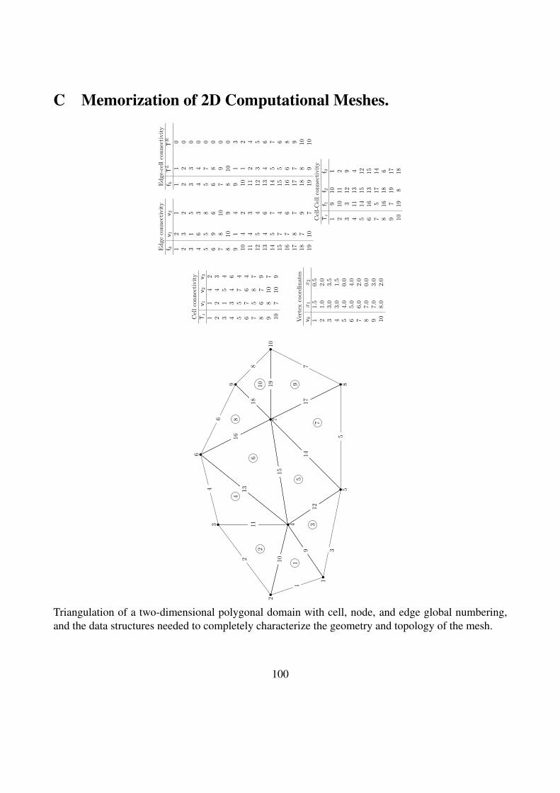
C Memorization of 2D Computational Meshes.
1
2
3 4
5
6
7
89
10
1
2
3
4
5
6
7
8
910
1
39
102
12
11
5
14
15
134
17
16
7
19
18
6
8
Cellconnectivity
Ti
v 1v 2
v 31
14
22
24
33
15
44
34
65
57
46
76
47
58
78
67
99
810
710
710
9
Vertexcoordinates
v kx1
x2
11.5
0.5
21.0
2.0
33.0
3.5
43.0
1.5
54.0
0.0
65.0
4.0
76.0
2.0
87.0
0.0
97.0
3.0
108.0
2.0
Edge
connectivity
f kv 1
v 21
21
23
23
15
46
35
58
69
67
810
810
99
14
10
42
11
43
12
54
13
46
14
57
15
74
16
76
17
87
18
79
19
10
7
Edge-cellconnectivity
f kTL
TR
11
02
20
33
04
40
57
06
80
79
08
100
91
310
12
11
24
12
35
13
46
14
57
15
56
16
68
17
79
18
810
19
910
Cell-Cellconnectivity
Ti
f 1f 2
f 31
910
12
10
11
23
312
94
11
13
45
14
15
12
616
13
15
75
17
14
816
18
69
719
17
1019
818
Triangulation of a two-dimensional polygonal domain with cell, node, and edge global numbering,and the data structures needed to completely characterize the geometry and topology of the mesh.
100

D Review of linear algebraIn the following a scalar number (integer, real or complex) will generally indicated using lowercaseGreek letters, e.g.:
α ∈ I β ∈ R α ∈ C.
A vector, identified as an ordered n-ple of numbers (e.g., reals) will be named using lowercase Englishletter, and we will use the following equivalent notations:
x ∈ Rn x =
x1
.
.
.xn
x = xi.
The number xi ∈ R is the i-th element (component) of vector x.A matrix is identified by a table of numbers (e.g., reals) with n rows and m columns. It will bedenoted with a uppercase letter of the English alphabet using the following equivalent notations:
A[n×m] A =
a11 . . . a1m
. . . .
. . . .
. . . .an1 . . . anm
A = aij.
The number aij ∈ R is the ij-th element (component) of matrix A. In most cases we will use squarematrices (m = n). A vector can be considered as a matrix with 1 column (m = 1). The use of acolumn vector is a convention, and we can define vectors more properly as element of vector spaces.However, we will always use the previous notation in the discussion of the properties of vectors andmatrices that are important for our developments.
Matrix sum. The sum of two matrices of the same dimension (row and column) is defined as thematrix have elements that are sums of the corresponding elements of the terms of the sum. In formula,given A,B,C ∈ Rn×m, we can write:
C = A±B := aij ± bij.
Product of a matrix by a scalar. The product of a matrix (or vector) by a scalar is defined againelement-wise as:
αA = αaij.
101

Transpose matrix. Given a matrix A ∈ Rn×m, the matrix obtained by exchanging rows withcolumns is called the transpose of matrix and is indicated as AT ∈ Rm×n:
A = aij AT = aji.
In the complex field A ∈ Cn×n the operation of transposition must be accompanied by the operationof complex conjugation:
A = aij A∗ = AT = aji.
Zero (null) matrix. The zero matrix (vector) is a matrix with all elements equal to zero, and is the“identity” element of the sum:
A = 0⇐⇒ aij = 0 i, j = 1, . . . , n.
Identity matrix. The identity matrix I is a matrix with unitary diagonal elements and zero non-diagonal elements:
I[n×n] I :=
1 0 . . . 0 00 1 . . . 0 0. . . . . .0 0 . . . 1 00 0 . . . 0 1
.
Positive (non-negative) matrix. A matrix is called “positive” (“non-negative”) 8 if all the elementsare non-negative with at least one positive element:
A > 0⇒ aij ≥ 0.
Scalar product between two vectors. Given two vectors x, y ∈ Rn, the sum of the product ofcorresponding elements is called the “scalar product” between x and y:
xTy = 〈x, y〉 = x · y :=n∑i=1
xiyi.
We will use also different notation such as:
〈x, y〉 or x · y.8The property of a matrix of being positive should not be confused with the property of being positive definite that will
be seen in a few paragraphs.
102

A more formal definition of a scalar product (or inner product) is as follows. Given a vector spaceV ⊂ Cn ( o Rn), the scalar (or inner) product between two elements x, y ∈ V , denoted by 〈x, y〉, is amap:
〈·, ·〉 : V × V → C ( o R)
that satisfies the following defining properties:
• (Hermitian Symmetry) 〈x, y〉 = 〈y, x〉 where (·) denotes complex conjugate;
• (Linearity) 〈αx+ βy, z〉 = α 〈x, z〉+ β 〈y, z〉;
• (positivity) 〈x, x〉 > 0 for each x ∈ Cn (or Rn) and 〈x, x〉 = 0 only if x = 0.
Matrix product. The product between two matrices, the row-by-column product, is given by thematrix whose components are the scalar products between the rows of the first matrix and the columnsof the second matrix (though of as vectors):
A[n×p] = aij B[p×m] = bij C[n×m] = cij
C = AB cij :=∑k=1,p
aikbkj, i = 1, . . . , n j = 1, . . . ,m.
The matrix-vector product is a special case of the matrix product with the vector though of as a n× 1matrix. It is easy to check that, in the real field Rn, the scalar product has the following property9:
〈x,Ay〉 =⟨ATx, y
⟩〈Ax, y〉 =
⟨x,ATy
⟩.
Determinant of a matrix. Given a square matrixA[n×n], the determinant det (A) is the scalar givenby the sum of all the products obtained taking as factors one element of each row and one element ofeach column:
det (A) :=∑±a1,i1a2,i2 · · · an,in ,
where i1, i2, . . . , in are different permutations of the first n natural numbers and the sign is given bythe order of the permutation.
Trace of a matrix. Given a square matrix A[n×n], the trace Tr (A) is the scalar given by the sum ofall the diagonal elements
Tr (A) :=∑i=1
naii.
9Obviously, in Rn the scalar product is commutative, i.e.: 〈x,Ay〉 = 〈Ay, x〉 or xTAy = (Ay)Tx
103

Inverse of a square matrix. Given a square matrix A[n×n], with det (A) 6= 0, the “inverse” matrixA−1 is the matrix such that:
A−1A = AA−1 = I.
Singular matrix. A matrix is “singular” if it does not have an inverse. A singular matrix has a nulldeterminant and vice-versa.
Orthogonal or unitary matrix. A matrix is orthogonal or unitary if:
UT = U−1.
Properties of operations between square matrices.
1. AB 6= BA (Matrices for which the commutativity properties of the product is valid are called“commutative”).
2. A+B = B + A
3. (A+B) + C = A+ (B + C)
4. (AB)C = A(BC)
5. A(B + C) = AB +BC; (A+B)C = AC +BC
6. (AB)T = BTAT
7. (AB)−1 = B−1A−1
8. (AT )−1 = (A−1)T .
Symmetric Matrix. A matrix is called “symmetric” if it is equal to its transpose:
A = AT ;
it is called “skew-symmetric” if it is the negative of its transpose:
A = −AT .
Every matrix can be decomposed as the sum of its symmetric and skew-symmetric parts:
A =1
2(A+ AT ) +
1
2(A− AT ).
104
Positive Definite Matrix. A matrix A[n×n] is called “positive definite” (“semi-positive definite”) if:
xTAx = 〈x,Ax〉 > 0 (〈x,Ax〉 ≥ 0) ∀x 6= 0.
M-Matrix. A matrix is of type M or an M -matrix if:
1. it is non-singular;
2. all the diagonal elements are positive;
3. all the extra-diagonal elements are negative or zero.
An M -matrix has the important property that its inverse is a positive matrix.
D.1 Vector spaces, linear independence, basisVector Space. A vector space V over the scalar field R is a set of vectors where the operation ofsum between two vectors and multiplication by a (real) scalar are defined. These operations mustsatisfy the following axioms10 for every x, y ∈ V and α, α1, α2 ∈ R:
1. x+ y = y + x;
2. x+ (y + z) = (x+ y) + z;
3. the “zero” vector is the identity element of the sum between vectors: x+ 0 = 0 + x = x;
4. for each x there exists a unique vector −x such that x+ (−x) = 0;
5. 1x = x;
6. (α1α2)x = α1(α2x);
7. α(x+ y) = αx+ αy;
8. (α1 + α2)x = α1x+ α2x.
Example of vector spaces:
• Rk, the set of all vectors with k components with the classic operations of sum and product bya scalar (the k-dimensional Eucledian space);
• R∞ the set of vectors with infinite elements (with the same operations as before);
10We note that these properties act in such a way that most of the elementary operations that we usually carry out in thescalar field will be valid also in a vector space.
105

• the space of matrices m× n; in this case the elements of the vector space are matrices and theoperations are the usual ones;
• the space of continuous functions f(x) defined in the interval 0 ≤ x ≤ 1 (examples of elementsof this space are f(x) = x2 and g(x) = sin(x), for which we have (f + g)(x) = x2 + sin(x)and every multiple such as 3x2 or − sin(x) belong to the same space). The vectors of the spaceare in this case functions and thus have “infinite dimensions”.
Vector Subspace. A subspace S ⊂ V of the vector space V is a subset of V with the followingproperties:
1. the sum of every two vectors x, y ∈ S, z = x+ y, is an element of S;
2. the product of every x ∈ S by a scalar α ∈ R is an element of S: z = αx, z ∈ S.
We say that the subspace S is “closed” under the operations of addition and multiplication by a scalar.An example of a vector subspace is a plane (affine to the vector space R2 is thought isolated but it iscontained in R3).
Linear independence. We say that k vectors vi are “linear independent” if all the linear combina-tions of these vectors (except the trivial combination all zero coefficients) result in a non-zero vector:
α1v1 + α2v2 + · · ·+ αkvk 6= 0 excluding the case α1 = α2 = · · · = αk = 0.
Otherwise the vectors are said “linearly dependent”.The following property is true: a set of k vectors belonging to Rm must necessarily be linearly depen-dent if k > m.
Span. If a vector space V is formed by all linear combinations of the vectors v1, v2, . . . , vn, we saythat these vectors “generate” the space V and we write:
V = spanv1, v2, . . . , vn.
In other words, every vector of V other than v1, v2, . . . , vn can be written as a linear combination ofthe generating vectors:
w ∈ V ⇒ w = α1v1 + . . . αnvn =n∑i=1
α1v1.
Basis. A minimal set of vectors is a basis of the vector space V if:
1. the vectors are linearly independent;
2. the vectors generate V .
106
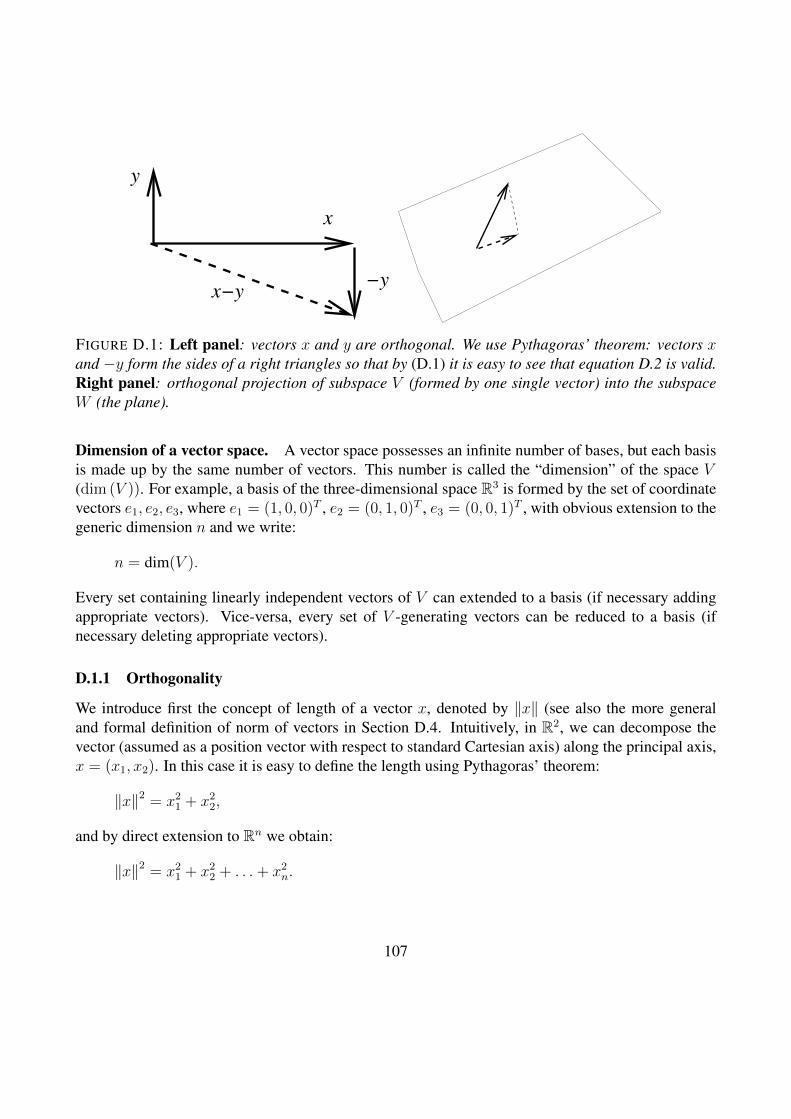
−y
x
y
x−y
FIGURE D.1: Left panel: vectors x and y are orthogonal. We use Pythagoras’ theorem: vectors xand −y form the sides of a right triangles so that by (D.1) it is easy to see that equation D.2 is valid.Right panel: orthogonal projection of subspace V (formed by one single vector) into the subspaceW (the plane).
Dimension of a vector space. A vector space possesses an infinite number of bases, but each basisis made up by the same number of vectors. This number is called the “dimension” of the space V(dim (V )). For example, a basis of the three-dimensional space R3 is formed by the set of coordinatevectors e1, e2, e3, where e1 = (1, 0, 0)T , e2 = (0, 1, 0)T , e3 = (0, 0, 1)T , with obvious extension to thegeneric dimension n and we write:
n = dim(V ).
Every set containing linearly independent vectors of V can extended to a basis (if necessary addingappropriate vectors). Vice-versa, every set of V -generating vectors can be reduced to a basis (ifnecessary deleting appropriate vectors).
D.1.1 Orthogonality
We introduce first the concept of length of a vector x, denoted by ‖x‖ (see also the more generaland formal definition of norm of vectors in Section D.4. Intuitively, in R2, we can decompose thevector (assumed as a position vector with respect to standard Cartesian axis) along the principal axis,x = (x1, x2). In this case it is easy to define the length using Pythagoras’ theorem:
‖x‖2 = x21 + x2
2,
and by direct extension to Rn we obtain:
‖x‖2 = x21 + x2
2 + . . .+ x2n.
107

Orthogonal vectors. Two vectors x and y in R2 are orthogonal if the angle formed by their inter-section is equal to π/2 (Figure D.1):
‖x‖2 + ‖y‖2 = ‖x− y‖2 . (D.1)
If we write the previous equation component-wise we have immediately that the products betweencomponents in different positions must be zero (sum of double-products), from which we have thegeneral condition of orthogonality in Rh:
xTy = 〈x, y〉 = 0. (D.2)
This quantity is the scalar product. We can show directly that if n vectors are all orthogonal then theyare linearly independent.
Orthogonal Spaces Two subspaces V and W of Rn are “orthogonal” if every vector v ∈ V isorthogonal to every vector w ∈ W .
Orthogonal Complement. Let V ⊂ Rn, the space of all vectors that are orthogonal to all vectorsof V is called the “orthogonal complement” of V and is denoted by V ⊥.
Null Space and Range of a Matrix. The set of all vectors x ∈ Rn such that Ax = 0 is called the“null space” or “kernel” of matrix A and is denoted by Ker (A).The set of all vectors x ∈ Rn such that Ax 6= 0 is called “image” or “range” of matrix A and isdenoted by Ran (A).A fundamental theorem states that:
dim (Ker (A)) + dim (Ran (A)) = n,
and the rank of A is equal to the dimension of Ran (A).
D.2 Projection Operators.A “projection operator”, or “projector”, P is a linear transformation P : Rn → Rn that is idempotent,i.e., such that:
P 2 = P. (D.3)
An easy example of a projection operation is the projection of a three-dimensional vector into acoordinate plane: given vector x = (x1, x2, x3)T , the projector that transforms this vector into x =(x1, x2, 0)T is represented by the matrix:
P =
1 0 00 1 00 0 0
.108
P is obviously idempotent:
P
x1
x2
x3
=
x1
x2
0
i.e., P 2x = P (Px) = Px = x.Here we list some properties of a projector P :
1. if P is a projector, then also (I − P ) is a projector;
2. Ker (P ) = Ran (I − P );
3. Ker (P ) ∩ Ran (P ) = 0 (the zero vector).
4. Rn = Ker (P )⊕ Ran (P );
In fact, if P satisfies (D.3), we immediately obtain: (I−P )(I−P )x = (I+P 2− 2P )x = (I−P )x,which shows the first property. The second property is an immediate consequence of the first. Thethird property derives directly from the property of idempotence: if x ∈ Ran (P ) then Px = x; ifx ∈ Ker (P ) then Px = 0, so that x = Px = 0. Obviously, every element of Rn can be written asx = Px+ (I − P )x, that demonstrates the fourth property.Let M ⊂ Rn and S ⊂ Rn, and let L = S⊥. Then the projector P on M orthogonal to the subspace Lis the linear transformation u = Px (∀x ∈ Rn) such that:
u ∈M (D.4)x− u ⊥ L (D.5)
These relationships determine the m = Rank (P ) = dim (M) conditions and corresponding degreesof freedom that define Px. It can be shown that these relationships determine uniquely the projectorP . In other words, given two subspaces M and L of dimension m it is always possible to define aprojector P on M orthogonal to L via conditions (D.4) and (D.5). We have the following:
Lemma D.1. Given two subspaces of Rn, M e L, both having dimension m, the following conditionsare equivalent:
1. no vectors of M are orthogonal to L
2. for each x ∈ Rn there exists a unique vector u that satisfies (D.4) and (D.5).
Proof. The first condition is equivalent to:
M ∩ L⊥ = 0.
109
Since L and L⊥ have dimensions n e n−m, then:
Rn = M ⊕ L⊥.
Hence, for every x there is a unique vector u ∈M such that:
x = u+ w w = x− u ∈ L⊥.
Matrix Representation. Practical work with the tools described above needs the definition ofthe basis to represent the projectors. Hence, we need to find two set of basis vectors, one for MV = [v1, . . . , vm], and one for L W = [w1, . . . , wm]. These bases are said to be “bi-orthogonal” if〈vi, wj〉 = δij , or in matrix form: W TV = I . We call V y the representation of vector Px under thebasis V . The orthogonality condition x− Px ⊥ L can be written as:
〈(x− V y), wj〉 = 0 per j = 1, . . . ,m,
or:
W T (x− V y) = 0.
If the bases V and W are bi-orthogonal then y = W Tx, and thus Px = VW Tx. From these last twoequation we immediately derive the matrix representation of the projector operator:
P = VW T .
When the two basis are not bi-orthogonal, the expression becomes:
P = V (W TV )−1W T .
From lemma D.1, we immediately conclude that matrix W TV has dimension m × m and is non-singular.
Orthogonal Projection. Given V ∈ Rn and W ∈ Rn, one of the following equivalent statementsimplies that V and W are orthogonal:
1. W = V ⊥ (W is formed by all vectors orthogonal to V );
2. V = W⊥ (V is formed by all vectors orthogonal to W );
3. V e W are orthogonal and dim V + dim W = n.
110

The orthogonal projection of a vector x ∈ V1 along the direction of vector y ∈ V2 is given by thevector:
y = 〈x, y〉 y = yyTv = Pv
A projector P is “orthogonal” if the two subspaces M and L are equal, and hence Ker (P ) =Ran (P )⊥. A projector that is not orthogonal is called “oblique”. We remark that a projector canbe characterized in the following manner. For each x ∈ Rn:
Px ∈M,
x− Px = (I − P )x ⊥M,
or in other words:
Px ∈M〈(I − P )x, y〉 = 0 ∀y ∈M.
We immediately derive the following:
Proposition D.2. A projector is orthogonal if and only if it is symmetric (Hermitian).
Proof. The transformation P T , defined by the adjoint transformation P by⟨P Tx, y
⟩= 〈x, Py〉 ∀x, y
is also a projector. In fact:⟨(P T )2x, y
⟩=⟨P Tx, Py
⟩=⟨x, P 2y
⟩= 〈x, Py〉 =
⟨P Tx, y
⟩.
Hence
Ker(P T)
= Ran (P )⊥ ,
Ker (P ) = Ran(P T)⊥.
By definition, a projector is orthogonal if Ker (P ) = Ran (P )⊥: if P = P T then P is orthogonal. Onthe other hand, and orthogonal P is such that Ker (P ) = Ker
(P T)
and Ran (P ) = Ran(P T). Since
P is a projector and thus it is uniquely defined by its null space and range, we deduce at once thatP = P T .
111
Optimality Properties of an Orthogonal Projector.
Lemma D.3. Let M ⊂ Rn and P a projector on M . Then for each x ∈ Rn:
‖x− Px‖ ≤ ‖x− y‖ ∀y ∈M.
Proof. The orthogonality conditions yield:
‖x− y‖22 = ‖x− Px+ (Px− y)‖2
2 = ‖x− Px‖22 + ‖Px− y‖2
2 .
from which immediately we get ‖x− Px‖2 ≤ ‖x− y‖2 with equality holding for y = Px.
Corollary D.4. Let M be a subspace and x a vector in Rn. Then:
miny∈M‖x− y‖2 = ‖x− y‖2
if and only if the following conditions are both satisfied:
y ∈M, x− y ⊥M.
D.3 Eigenvalues and EigenvectorsA scalar λ and a vector r 6= 0 are called a “eigenvalue” and a “eigenvector” of the (square) matrix Aif:
Ar = λr. (D.6)
From this definition it follows that:
(A− λI)r = 0 ⇒ P (λ) = det (A− λI) = 0. (D.7)
From (D.6), eigenvectors are defined up to a multiplicative constant, i.e., if r is a eigenvector then αris also a eigenvector. From (D.7) we see that the eigenvalues are the roots of a polynomial of degree nwith real coefficients (if A has real elements). Hence, there are n eigenvalues λ1, λ2, . . . , λn (a poly-nomial of degree n has n roots) not necessarily distinct. Correspondingly, we have n eigenvectors.We also have the following properties of the eigenvalues of A:
λ ∈ Cn∑i=1
λi =n∑i=1
aii = Tr An∏i=1
λi = det (A) Amr = λmr.
If a eigenvalue of A is zero (λ = 0) then matrix A is singular (det (A) = 0). Following standardnotation, the set of all eigenvalues of A is denoted by λ(A) and is called the “spectrum” of A. It iscommon to order the eigenvalues in decreasing order of their modulus:
| λ1 |≥| λ2 |≥ . . . ≥| λn |,so that λ1(A) and λn(A) denote the eigenvalues ofA having maximum and minimum moduli, respec-tively. The “spectral radius” of A is ρ(A) =| λ1(A) |.
112
Similarity Transformation. A matrix B is obtained from matrix A via a “similarity transforma-tion” if there exists a non-singular matrix S such that:
B = S−1AS.
Matrices B and A have the same eigenvalues and eigenvectors transformed by the same matrix S. Infact, we can write:
det (B − λI) = det(S−1AS − λS−1S
)= det
(S−1
)det (A− λI) det (S) = det (A− λI) ,
and so:
Br = λrAs = λs
⇒ S−1ASr = λrASr = λSr
⇒ s = Sr.
It is easy to check that:
λ(A) = λ(AT ) λ(AB) = λ(A−1ABA) = λ(BA). (D.8)
Given the diagonal matrix D having as diagonal elements the elements of A, then:
D = dij dij =
aii if i = j
0 if i 6= j.
It follows immediately that:
λ(D−1A) = (where S = D−12 ) = λ(D
12D−1AD−
12 ) = λ(D−
12AD−
12 ).
Matrix B = D−12AD−
12 is positive definite if and only if A is:
〈x,Bx〉 =⟨x,D−
12AD−
12x⟩
=⟨D−
12x,AD−
12x⟩> 0 ∀x 6= 0.
Property of a Symmetric Matrix and Diagonalization.
• The eigenvalues and eigenvectors of a symmetric matrix A are real.
• The eigenvalues and eigenvectors of a skew-symmetric matrix A are imaginary.
• If A is positive definite then λi > 0 for i = 1, . . . , n.
• A general square11 matrix A is said to be “diagonalizable” if there exists a nonsingular matrixU such that:
Λ = U−1AU (D.9)
is a diagonal matrix. It is easy to see that Λ = λii where λii = λi the eigenvalues of A, andthe columns of U are the corresponding eigenvectors ri.
11Not necessarily symmetric or Hermitian
113
• If A is SPD (Symmetric and Positive Definite), then it is diagonalizable and matrix U is unitary(U−1 = UT ). Since the columns of U are orthogonal, the eigenvectors of and SPD matrixsatisfy:
〈ri, rj〉6= 0 if i = j
= 0 if i 6= j;
but since the eigenvectors are defined up to a multiplicative constant, we can normalize each ofthem with respect to their Eucledian norm (length) to get:
〈ri, rj〉 =
1 if i = j
0 if i 6= j;
Hence, the eigenvectors of diagonalizable matrices form a basis for the vector space Rn. If Ais SPD this basis is orthonormal. In other words, all vectors in Rn can be expressed as linearcombination of the eigenvectors of A. We would like to stress that an orthonormal basis isalways numerically “well conditioned”.
Left and Right Eigenvectors. The eigenvectors defined by (D.6) are called the “right” eigenvectorsof A. We can also define “left” eigenvectors l (and corresponding eigenvalues) as:
lTA = µlT . (D.10)
By transposition, we obtain:
AT l = µl = λl,
which states that the left eigenvectors are the right eigenvectors of the transpose matrix AT and theleft and right eigenvalues coincide (µ = λ). Obviously, if the matrix is symmetric then left and righteigenvectors coincide 12.We have seen in the previous paragraph that every diagonalizable matrix has a complete set of eigen-vectors (complete in the sense that these eigenvectors span Rn). We can use left eigenvectors for thesame purpose: also the left eigenvectors span Rn, i.e., they form a basis for Rn, which is differentfrom the basis formed by the right eigenvectors. Given a diagonalizable real matrix A we denoteby ri and li the right and left eigenvectors, respectively. Since both eigenvectors are defined up to amultiplicative constant, we assume that they have been normalized so that ‖r‖2 = 1 and 〈li, rj〉 = δij ,where δij = 1 if i = j, δij = 0 if i 6= j. Then we collect the right eigenvectors as columns of thematrix U and the left eigenvectors as columns of the matrix V . These matrices (and thus the left andright eigenvectors) are “bi-orthogonal”:
V TU = I, 〈li, rj〉 = δij.
12Depending on notation, they may be the same up to transpose operation.
114

Hence, we can write:
V TAU = V TUΛ = ΛV TU = Λ.
We notice that V T = U−1, which shows that the previous equation is equivalent to (D.9). The set ofvectors collected in V T and U are called “dual” basis.Any vector x ∈ Rn = xi can be written as a linear combination of the right eigenvectors as follows:
x = c1r1 + c2r2 + . . .+ cnrn = Uc,
where c = ci is a vector of Rn. Since V T = U−1, we can invert the previous equation to obtain:
c = V Tx = (〈l1, x〉 , 〈l2, x〉 , . . . , 〈ln, x〉)T .In other words, the coefficients of the linear combination of right eigenvectors that forms vector x aregiven by the scalar products between the left eigenvectors and x itself:
ci = 〈li, x〉 . (D.11)
D.4 Norms of Vectors and MatricesVector Norms. The “norm” of a vector x is a real scalar such that:
1. ‖x‖ > 0, ‖x‖ = 0 if and only if x = 0;
2. given α ∈ R, ‖αx‖ =| α | ‖x‖;3. ‖x+ y‖ ≤ ‖x‖+ ‖y‖;
Examples of vector norms is the p-norm:
‖x‖p =
(n∑i=1
| xi |p)1/p
.
For p = 2 we have the classic Eucledian length of a vector, which is then a norm: ‖x‖2 =√〈x, x〉.
for p = ∞ we have the maximum norm ‖x‖∞ = maxi | xi |, while for p = 1 we have the absolutenorm ‖x‖1 =
∑ni=1 | xi |. For p = 2 the following Schwartz inequality holds:
〈x, y〉 ≤ ‖x‖2 ‖y‖2 .
Note that
‖x‖2 =√〈x, x〉.
Another norm that is often used is the “energy” norm. This is defined by the scalar product betweenthe vector x and the vector Ax, where matrix A is SPD13:
‖x‖A =√〈x,Ax〉.
13If A is not SPD, then the property 1 is not satisfied
115
Matrix Norm. A norm of matrix A is a real scalar such that:
1. ‖A‖ > 0, ‖A‖ = 0 if and only if A = 0;
2. given α ∈ R, ‖αA‖ =| α | ‖A‖;
3. ‖A+B‖ ≤ ‖A‖+ ‖B‖;
4. ‖AB‖ ≤ ‖A‖ ‖B‖;Example of matrix norms are:
• Frobenius norm: ‖A‖2 =√
Tr (ATA) =√∑
ij | aij |2;
• Spectral or Hilbert norm: ‖A‖ =√ρ(ATA) =
√| λ1(ATA) |.
Norm Induced by the Norm of a Vector (Compatible Norms). A matrix norm ‖A‖ is said to beinduced by (or be compatible with) the vector norm ‖x‖ if:
‖A‖ = supx 6=0
‖Ax‖‖x‖ .
The spectral norm is induced by the Eucledian norm of a vector. In fact, given a non-singular matrixA ∈ Rn×n, we can build the symmetric and positive definite matrix H = ATA. Since H is diagonal-izable, we can think of a generic nonzero vector x ∈ Rn as a linear combination of the eigenvectorsri of H:
x = c1r1 + c2r2 + . . .+ cnrn = Uc,
where the columns of matrix U are the eigenvectors of H (U = [r1, . . . , rn]), and c = ci. Since riare orthogonal, we have:
〈x,Hx〉 =⟨x, UΛUTx
⟩=⟨Uc, UΛUTUc
⟩≤ λ1(H) ‖x‖2
2 ,
from which we have immediately:
λ1(ATA) ≥ 〈Ax,Ax〉‖x‖2
2
=‖Ax‖2
2
‖x‖22
.
The proof is completed by taking square roots.14
14We could have done a lengthier proof by using vector components as follows:
〈x,Hx〉 = xTHx = (c1r1 + c2r2 + . . .+ cnrn)TH(c1r1 + c2r2 + . . .+ cnrn)
= λ1 | c1 |2 + . . .+ λn | cn |2
≤ λ1(| c1 |2 + . . .+ | cn |2) = λ1 ‖x‖22 .
116

Linear systems of equations. Given a non singular matrix A of dimension n × n and a vectorb ∈ Rn, we look for the vector x ∈ Rn that satisfies:
Ax = b.
The formal solution of this system is indicated with:
x∗ = A−1b.
However, the direct use of the inverse is in general never pursued in practice as the evaluation of A−1
is computationally very expansive15
Using an iterative method for solving the linear system one defines a sequence of iterate vectorsxk, k > 0, such that:
limk→∞
xk = x∗. (D.12)
The iteration terminates in practice for relatively small values of k. However, since we do not knowx∗ it will be impossible to theoretically satisfy the termination criterion exactly. For this reason, aniterative method terminates based on the “size” of the residual vector, defined as:
rk = b− Axk.
It is easy to see that the convergence condition (D.12) implies that the residual must converge to zeroas k →∞. Hence, in practical algorithms, the iteration stops when the norm of the residual is smallerthan a predetermined threshold, called “tolerance” generally denoted by τ . It is often more convenientand precise to use a relative termination criterion, requiring the termination of the iteration when theinitial residual has decreased by a factor τ :
‖rk‖‖r0‖
< τ.
Defining the error vector as the difference between the approximate and the real solutions, ek =xk − x∗, we can evaluate the relationship between error and residual as:
‖ek‖‖e0‖
≤ κ(A)‖rk‖‖r0‖
.
where k(A) = ‖A‖ ‖A−1‖ is called the “condition number” of matrix A. Indeed:
rk = b− Axk = −Aek,15The simplest way to evaluate the inverse of A is to solve n linear system using A as system matrix and the vectors
ej = 0, 0, . . . , 1, . . . , 0 as right hand side. There are actually other methods to evaluate an approximation to A−1 butthese are generally more expensive than solving a single linear system.
117
from which, using induced norms, we obtain:
‖ek‖ =∥∥A−1Aek
∥∥ ≤ ∥∥A−1∥∥ ‖Aek‖ =
∥∥A−1∥∥ ‖rk‖ ,
and:
‖r0‖ = ‖Ae0‖ ≤ ‖A‖ ‖e0‖ ,
and thus:
‖ek‖‖e0‖
≤∥∥A−1
∥∥ ‖A‖ ‖rk‖‖r0‖= κ(A)
‖rk‖‖r0‖
. (D.13)
This termination condition is not convenient as it depends on the initial solution x0. It is often easierto relate the norm of the current residual to the norm of the right hand side vector b, i.e.:
‖rk‖‖b‖ < τ.
The two conditions are equivalent whenever the initial solution is the zero vector x0 = 0 and thusr0 = b, a common choice in practical applications.In what follows we will often make reference at the following sample case:
Ax = b where A =
[3 22 6
]x =
[x1
x2
]b =
[2−8
](D.14)
having theoretical solution:
x∗ =
[2−2
].
We can make a geometrical interpretation of the above system in R2. The solution is the point ofintersection between the two lines having equations given by the two equations of the linear system(see Figure D.2).
D.5 Quadratic FormsGiven matrix A of dimensions n × n, a vector b ∈ Rn, and a scalar γ ∈ R, a quadratic form is afunction taking as variables vectors with components x1, x2, . . . , xn and returning real scalar values.In more precise terms, a quadratic form is a function f such that:
f : Rn → R
is defined by:
f(x) =1
2xTAx− bTx+ c =
1
2〈x,Ax〉 − 〈b, x〉+ c. (D.15)
118

-4 -2 2 4 6
-6
-4
-2
2
4
x1
x2
3x1 + 2x2 = 2
2x1 + 6x2 = 8
FIGURE D.2: Geometric interpretation of a linear system in R2. The solution is the point of intersec-tion of the two lines, i.e., the point identified by the vector x∗ = [2,−2]T .
We are interested in finding the point x ∈ Rn where f(x) is minimum. We say that f(x) as a minimumin x∗ if f(x∗) < f(x) for all x in the domain of f . We know that if all the partial derivatives of fare zero in x∗ then x∗ can be an extremizer, that is x∗ can be a point of minimum, maximum, or ofstationarity. For example, in R2, the function z = f(x, y) = x2 + y2 has a point of absolute minimumin (0, 0). On the other hand, the partial derivatives of the function z = f(x, y) = xy are both zero in(0, 0) but this point is not of minimum. In fact, all points (x, y) of the first and third quadrant (wherex and y have the same sign) are such that f(x, y) > 0 = f(0, 0), while all the points in the secondand fourth quadrants (where x and y have opposite signs) we have f(x, y) < 0 = f(0, 0).Given a vector v ∈ Rn and a scalar ε ∈ R we form a new vector x∗ + εv ∈ Rn. The vector x∗ is apoint of absolute minimum if:
f(x∗ + εv) > f(x∗) for each ε and each v.
In particular, this inequality should be satisfied for values of ε as small as possible. Hence we canwrite the condition of stationarity for f(x) as:
d
dε[f(x+ εv)] |ε=0 = 0,
that should be valid for all v ∈ Rn. Using the chain rule for the differentiation of function compositionapplied component-wise to the previous equation we have:
d
dεf(x1, x2, . . . , xn) =
∂f
∂x1
dx1
dε+∂f
∂x2
dx2
dε+ · · ·+ ∂f
∂xn
dxndε
=∂f
∂x1
v1 +∂f
∂x2
v2 + · · ·+ ∂f
∂xnvn.
119
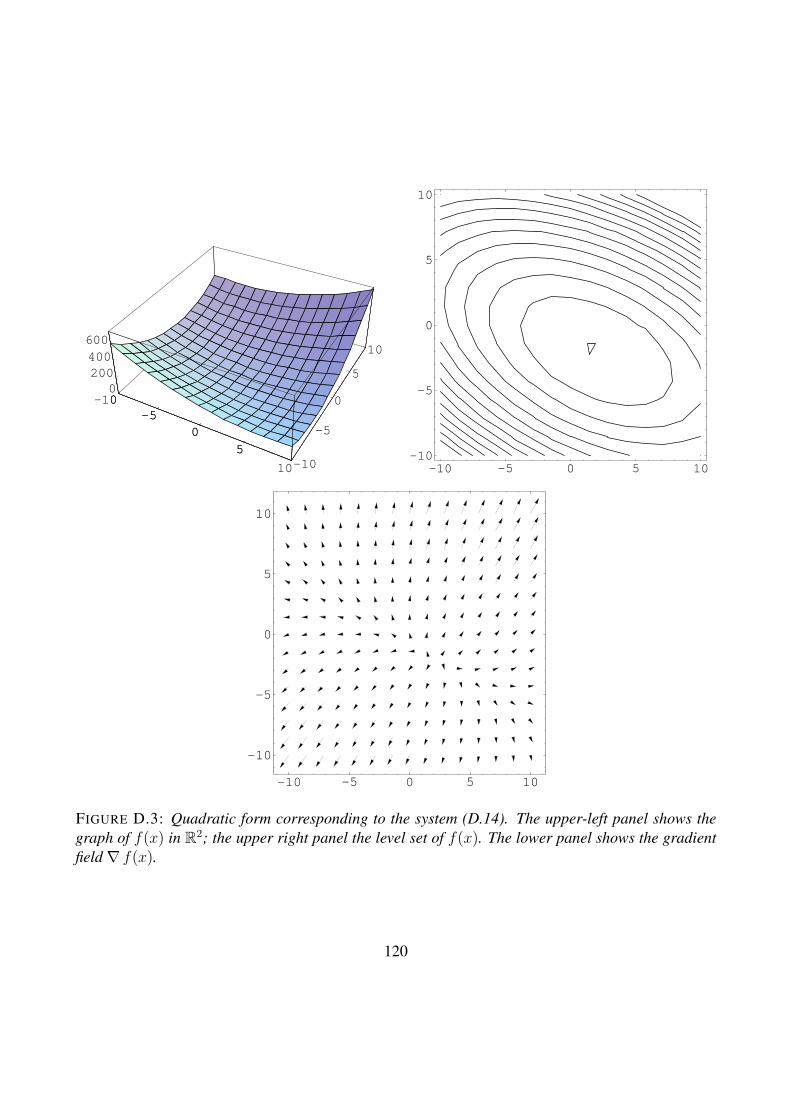
-10-5
0
5
10-10
-5
0
5
10
0200400600
-10-5
0
5
-10 -5 0 5 10-10
-5
0
5
10
-10 -5 0 5 10
-10
-5
0
5
10
FIGURE D.3: Quadratic form corresponding to the system (D.14). The upper-left panel shows thegraph of f(x) in R2; the upper right panel the level set of f(x). The lower panel shows the gradientfield∇ f(x).
120
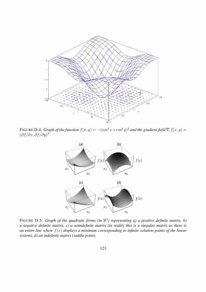
FIGURE D.4: Graph of the function f(x, y) = −(cos2 x+cos2 y)2 and the gradient field∇ f(x, y) =(∂f/∂x, ∂f/∂y)T
(c)
x1
x2
f(x)x1
(d)
x1
x2
f(x)x1
(a)
x1
x2
f(x)x1
(b)
x1
x2
f(x)x1
FIGURE D.5: Graph of the quadratic forms (in R2) representing a) a positive definite matrix, b)a negative definite matrix, c) a semidefinite matrix (in reality this is a singular matrix as there isan entire line where f(x) displays a minimum corresponding to infinite solution points of the linearsystem), d) an indefinite matrix (saddle point).
121

We define the gradient of the function f(x) as the vector of all partial derivatives (see Figures D.3and D.4):
∇ f(x) =
∂f∂x1∂f∂x2
.
.
.∂f∂xn
.
We can write the stationarity condition now directly as:d
dε[f(x+ εv)] |ε=0 = ∇ f(x) · v = 〈∇ f(x), v〉 = ∇ f(x)Tv = 0. (D.16)
We note that if ‖v‖ = 1 then 〈∇ f(x), v〉 = Dvf(x) can be interpreted as the directional derivative off in x along the direction identified by vector v. On the other hand, in the case of our quadratic formgiven by (D.15), we can write:
f(x+ εv) =1
2〈(x+ εv), A(x+ εv)〉 − 〈b, (x+ εv)〉+ c
=1
2
[〈x,Ax〉+ ε 〈v, Ax〉+ ε 〈x,Av〉+ ε2 〈v, Av〉
]− 〈b, x〉 − ε 〈b, v〉+ c,
from which we obtain:d
dε[f(x+ εv)] |ε=0 =
1
2[〈v, Ax〉+ 〈x,Av〉]− 〈b, v〉
=
⟨A+ AT
2x, v
⟩− 〈b, v〉 = 0.
As a consequence, we have:
∇ f(x) =A+ AT
2x− b (D.17)(A+ AT
2x − b
)⊥ v,
and we note that the last equation is valid for all v ∈ Rn, from which we find immediately:
A+ AT
2x = b,
and if A = AT the condition for a stationarity of (D.16) can be written as:
∇ f(x) = Ax− b (D.18)Ax = b.
We see then that if A = AT the quadratic form f(x) has a point of stationarity on the point of Rn
that solves the system Ax = b, while if A is indefinite but non singular then the point of stationaritycorresponds to the solution of the linear system 1
2(A+ AT )x = b.
122
D.6 Symmetric case A = AT
We can see that the stationarity point of f(x) defined above is a global minimum if and only if A issymmetric and positive definite. In fact, x∗ is a point of global minimum if f(x∗ + e) > f(x∗) for allvectors e ∈ Rn. Hence:
f(x∗ + e) =1
2〈A(x∗ + e), (x∗ + e)〉 − 〈b, (x∗ + e)〉+ c
=1
2[〈Ax∗, x∗〉+ 〈Ax∗, e〉+ 〈Ae, x∗〉+ 〈Ae, e〉]− 〈b, x∗〉 − 〈b, e〉+ c
=1
2〈Ax∗, x∗〉 − 〈b, x∗〉+ c+ 〈Ax∗, e〉+
1
2〈Ae, e〉 − 〈b, e〉
= f(x∗) +1
2〈Ae, e〉 ,
where we have used the fact that if A = AT then 〈Az,w〉 = 〈z, Aw〉. If A is also positive definite,then 〈Ae, e〉 > 0 from which we have immediately that f(x∗) is an absolute minimum.Figure D.3 shows the graph of f(x) and its gradient field ∇ f(x) in the case of the linear systemdefined by equation (D.14) that has a symmetric system matrix A. We note that the level lines thatrepresent f(x) in the plane (x1, x2) (Figure D.3 upper left) are ellipses with principal axes that aregiven by the (normalized) eigenvectors of A. In Rn these ellipses are actually hyper-ellipsoids andthe level lines are actually n-dimensional hyper-surfaces. In this case, the geometrical interpretation,although not being representable in a graphical object, remains exactly the same. In other words,the equation f(x) = C represents an hyper-ellipsoid in Rn and the center of this ellipsoid coincidewith the solution of the linear system 16. This fact can be easily understood if we work in a differentreference frame. To this aim, we start by noting that an approximate solution of our linear systemxk 6= x∗ is affected by an error defined as:
ek = xk − x∗.
We make now the following change of variables:
ek = Uz, (D.19)
where z is the new variable and U is the matrix whose columns collect the eigenvectors ri of Aordered according to the decreasing order of the eigenvalues (that are always positive). Matrix U isunitary (or orthogonal)17 and thus U−1 = UT . The new reference system has the origin located in thecenter of the hyper-ellipsoid and the coordinate axis coincide with the eigenvectors of A, so that wecan re-write our quadratic form as:
Φ(ek) = 〈ek, Aek〉 = 〈Uz,AUz〉 = zTΛz = 〈z,Λz〉 ,16Note that the graph of z = f(x) is represented in Rn+1.17Recall that A is symmetric and positive definite and thus is diagonalizable, i.e., the eigenvectors of A span the vector
space Rn.
123

whose level surfaces are represented by the equation:
λ1z21 + λ2z
22 + . . .+ λnz
2n = cost,
or:
z21
costλ1
+z2
2
costλ2
+ · · · z2n
costλn
= 1. (D.20)
This is the equation (in canonical form) of the hyper-ellipsoid with semi-axes have the length:
a1 =
√costλ1
, a2 =
√costλ2
, . . . , an =
√costλn
We note that the quadratic form Φ(·) has a point of minimum in the null vector, i.e., ek = xk−x∗ = 0,that corresponds to the minimum of f(·) written in the new reference frame, i.e., the solution of thelinear system. In fact:
f(xk) = f(x∗ + ek) = f(x∗) +1
2〈ek, Aek〉 =
1
2Φ(ek)
We have shown that the problem of finding the solution of the linear system Ax = b is equivalent tothe problem of finding the minimum of the quadratic form f(x). The problem is also equivalent toimpose the orthogonality between the residual and all vectors of Rn. In other words, for symmetricmatrices, the following problems are equivalent:
Problem D.5 (Linear system).Find x ∈ Rn such that:
Ax = b. (S)
Problem D.6 (Minimization (Ritz)).Find x ∈ Rn such that:
F (x) ≤ F (v) ∀v ∈ Rn. (M)
Problem D.7 (Variational (Galerkin)).Find x ∈ Rn such that:
〈b− Ax, v〉 = 0 ∀v ∈ Rn. (V)
124
References[1] A. Bressan. Sistemi iperbolici di leggi di conservazione. Bollettino della Unione Matematica
Italiana-B, 3-B(3):635–656, 2000.
[2] A. Bressan. Hyperbolic conservation laws: An illustrated tutorial. Lecture Notes, Departmentof Mathematics, Penn State University, USA, December 2009.
[3] H. S. Carslaw and J. C. Jaeger. Conduction of Heat in Solids. Oxford University Press, USA,1986.
[4] L. C. Evans. Partial differential equations, volume 19 of Graduate studies in mathematics.American Mathematical Society, Providence (R.I.), 2010.
[5] R. Eymard, T. Gallouet, and R. Herbin. Finite volume methods. In C. Ph. and L. J. L., editors,Handbook of numerical analysis, volume VII, pages 713–1020. North-Holland, Amsterdam,2000.
[6] C. Hirsch. Numerical computation of internal and external flows. volume 1. , fundamentals ofcomputational fluid dynamics. Butterworth-Heinemann, Amsterdam, Boston, London, 2007.ISBN 978-0-7506-6594-0.
[7] F. John. Partial differential equations; 3rd ed. Appl. Math. Sci. Springer, New York, NY, 1978.
[8] P. D. Lax. Hyperbolic systems of conservation laws ii. Comm. Pure Appl. Math., 10:537–566,1957. doi: 10.1002/cpa.3160100406.
[9] R. J. LeVeque. Numerical methods for conservation laws. Lectures in mathematics : ETHZrich. Birkhuser, Basel, Boston, Berlin, 1992. ISBN 978-3-7643-2723-1. URL http://opac.inria.fr/record=b1089678. Autres tirages : 1994, 1999, 2006, 2008.
[10] T.-P. Liu. The entropy condition and the admissibility of shocks. Journal of MathematicalAnalysis and Applications, 53(1):78 – 88, 1976. ISSN 0022-247X. doi: 10.1016/0022-247X(76)90146-3.
[11] A. Logg. Efficient representation of computational meshes. International Journal of Computa-tional Science and Engineering, 4(4):283, 2009.
[12] E. F. Toro. Riemann Solvers and Numerical Methods for Fluid Dynamics. Springer-Verlag,Berlin, Heidelberg, 2009.
125