nova school of business and economics - run.unl.pt · nova school of business and economics...
TRANSCRIPT
Nova School Of Business and Economics
Econometric approach for forecasting stock indices price
Author:Angelo Migliorino
Supervisor:Joao Amaro De Matos
May 25, 2017

Angelo Migliorino
List of Tables1 Stock Indices . . . . . . . . . . . . . . . . . . . . . . . . . . . . . . . . . . 92 GBM NKY out of sample . . . . . . . . . . . . . . . . . . . . . . . . . . . 133 GBM UK out of sample . . . . . . . . . . . . . . . . . . . . . . . . . . . . 144 GBM ATX out of sample . . . . . . . . . . . . . . . . . . . . . . . . . . . . 145 GBM DAX out of sample . . . . . . . . . . . . . . . . . . . . . . . . . . . 156 Resume indices . . . . . . . . . . . . . . . . . . . . . . . . . . . . . . . . . 187 S1 NKY out of sample . . . . . . . . . . . . . . . . . . . . . . . . . . . . . 198 S1 UK out of sample . . . . . . . . . . . . . . . . . . . . . . . . . . . . . . 199 S1 ATX out of sample . . . . . . . . . . . . . . . . . . . . . . . . . . . . . 2010 S1 DAX out of sample . . . . . . . . . . . . . . . . . . . . . . . . . . . . . 2011 S2 UK out of sample . . . . . . . . . . . . . . . . . . . . . . . . . . . . . . 2112 S2 NKY out of sample . . . . . . . . . . . . . . . . . . . . . . . . . . . . . 2213 S2 DAX out of sample . . . . . . . . . . . . . . . . . . . . . . . . . . . . . 2214 S2 ATX out of sample . . . . . . . . . . . . . . . . . . . . . . . . . . . . . 22
Contents1 Introduction 3
2 Multi-factor models 62.1 Three-Factor Model by Fama and French . . . . . . . . . . . . . . . . . . . 62.2 Four-Factor Model by Carharth . . . . . . . . . . . . . . . . . . . . . . . . 82.3 Five-Factors model by Fama and French . . . . . . . . . . . . . . . . . . . 8
3 Data 9
4 Buy And Hold 11
5 Geometric Brownian motion 115.1 Geometric Brownian motion strategy results . . . . . . . . . . . . . . . . . 13
6 Alternative Econometric Models 166.1 Methodology . . . . . . . . . . . . . . . . . . . . . . . . . . . . . . . . . . 166.2 Alternative model Results . . . . . . . . . . . . . . . . . . . . . . . . . . . 18
6.2.1 Simple Strategy . . . . . . . . . . . . . . . . . . . . . . . . . . . . . 186.2.2 Aggressive Strategy . . . . . . . . . . . . . . . . . . . . . . . . . . . 21
7 Conclusion 23
1

Angelo Migliorino
Abstract
This work proposes to build a profitable dynamic trading strategy. In order to
do that it is necessary to forecast the future stock indices prices. First we exploit
the forecast power of stock indices assuming that they follow a Geometric Brownian
motion. Next, we present an alternative forecasting model that involves cross sec-
tional regression between indices. The latter proves to be more profitable on average
than the former.
Keywords: cross sectional regressions, stock indices, stochastic processes, trad-
ing strategies
2
Angelo Migliorino
1 Introduction
Einstein used to say that God does not play dices with the Universe. In the early 1900s
the idea of quantum physics was born, revolutionizing the deterministic concept of nature.
As a byproduct of the quantum physics success, there was the initial impression that all
the natural phenomena were governed by probabilistic laws. Einstein argued that nature
should evolve according to deterministic mathematical laws. The complexity of nature
and of all these deterministic rules lead us to use probabilistic explanations of whatever
is observed - not because the underlying phenomena are intrinsically probabilistic, but
simply to hide the ignorance of the true mechanisms.
This paper is based on the idea that any financial market follows a logical structure where
the underlying laws of demand and supply determine its outcome. On the top of that
basic mechanism, there are random fluctuations. In other words, God rolls dices on the
top of a deterministic system, and those who know how to assess this specific randomness
will have more foreshadowing power. The objective of this work is to show that, by con-
sidering this additional randomness, it is possible to improve drastically the forecasting
power of future stock indices and build a subsequent more efficient strategy.
As referred in Kim and Han (2016), there are three alternative approaches to best fore-
cast stock prices: technical analysis, fundamental analysis and time series. As defined by
Murphy (1999), technical analysis forecasts future price trends mainly studying charts.
One of the most famous strategies is based on the Relative Strength Index1 (an index that
can take value 0 ≤ RSI ≤ 100). Menkhoff and Taylor (2007) studied the literature and
the reasons of using technical analysis in foreign exchange market. Using moving averages1Go long on the asset that are oversold (i.e. RSI<30) and short on the asset that are overbought (i.e.
RSI>70)
3

Angelo Migliorino
should be profitable as well. However, strong empirical evidence says that technical anal-
ysis can not be used to predict excess return. Daniotti (2012) studied a method referred
to the cross of two moving averages. Applying this method to three equity indices2 it
has resulted to be not profitable after transaction costs. The overall result is quite disap-
pointing since it did not outperform a simple buy and hold strategy.
The fundamental analysis, instead, tries to forecast returns looking at the intrinsic value
of a company as depending on macroeconomic (e.g. overall economy and industry condi-
tions) and microeconomic factors (e.g. financial conditions and company management).
Predicting excess returns using past information contradicts the Efficient Market Hypothe-
sis as defined by Fama (1969). There are however many models based on this fundamental
analysis assuming that markets are inefficient to some extent. One of the first models used
to do that (see Ang (2014)) is the Capital Asset Pricing Model (CAPM) 3. Many authors
tested the relationship
Ri,t+1 = α + βRm,t+1 + εt+1. (1)
Under the CAPM null hypothesis the expected result should be α = 0 and β = 1. Un-
fortunately, regressing a portfolio of US stocks and the S&P 500, the α resulted too large
and the R2 of the regression too small. In order to better explain the excess stock returns
Fama and French (1993) added two risky factors related to size and value of the portfolios
(namely the so-called SMB and HML factors). This is the model that seems to better
explain portfolio excess returns in terms of fundamental analysis.
Models that try to predict excess returns use time series data. A time series is a par-2Dow Jones Euro Stoxx for Europe, the S&P 500 for the USA and the Topix for Japan3it has been developed by Treynor (1961), Sharpe (1964), Lintner (1965), and Mossin (1966), based
on Harry Markowitz (1952)
4

Angelo Migliorino
ticular realization of a stochastic process, which is a set of random variables indexed by
time (Stirzaker (2005)). A stochastic process is said to be discrete if it is a measurable
set of random variables, and continuous if it is a non countable set of random variables.
A time series {xt} is thus a sample path of the underlying stochastic process, and can be
either discrete or continuous, depending on whether the series is recorded on discrete or
continuous time as defined in (Brockwell and Davis (2016)).
The literature on using continuous time models to predict prices and backtesting invest-
ment strategies is summarized by Sonono and Mashele (2015). This paper contributes by
proposing an alternative continuous-time model that uses multivariate rolling regressions
and fitted values to predict future prices. For each implemented strategy the results are
back-tested.
This paper is structured as follows. Next section presents the most important factor
models, connected with the fundamental analysis. The third section explains the data
set and presents the computation for every implemented strategy. The fourth section
brings the result of a simple buy and hold strategy, used as a benchmark. In the fifth
paragraph, the attention is switched to the underlying stochastic process, the Geometric
Brownian motion. Additionally, the backtesting of a potential strategy involving GBM
is computed. The sixth section provides an alternative model to forecast future indices
price. The associated backtesting strategy results provide evidence that this new model
beats the Geometric Brownian motion hypothesis and the buy and hold one. Last section
concludes.
5
Angelo Migliorino
2 Multi-factor models
One of the first models that exploited the trade-off between risk and return, thus explain-
ing portfolio returns, was the CAPM. Since in this model all the efficient portfolios are well
diversified, the systematic risk is the only one to be priced. The model itself states that
the market portfolio, with respect to which the systematic risk is measured, is efficient.
It thus follows that the expected excess return on a particular asset is a linear function of
its systematic risk, as measured by cov(σmσi)σ2m
(see Ericsson and Karlsson (2004)).
The CAPM is consistent with a single factor market model where the portfolio returns
are explained by the market portfolio. As such, the market return variable captures all
the systematic risk (see also Campbell et al. (1997)). This model has been used as a
workhorse of finance, particularly in capital budgeting decisions. As it is said in the first
section this model does not allow to best forecast future portfolio returns. If an investor
is willing to use a multi-factor model he is implying that factors, individually, explain the
systematic risk (Berk and DeMarzo (2007)). The general equation of a multi-factor model
is the following:
Rp = α +N∑n=1
βFni RFn + ε
where the βs are the coefficients for each factor. By taking expectations it follows that
summing the excess return of every factor, multiplied by the Beta 4, it is possible to obtain
the asset risk premium (Berk and DeMarzo (2007)).
2.1 Three-Factor Model by Fama and French
Multi-factor models pick variables that may best predict average returns and capture risk
premiums. Fama and French (1993) elaborated one of the most used models in empirical4Sensitivity of the asset with that explanatory factor
6
Angelo Migliorino
research and industry application (see (Bodie et al., 2014)):
Rp = α + βmRM + β2SMB + β3HML+ ε, (2)
where SMB (Small minus Big) identifies the market capitalization and HML (High minus
Low) describes the book-to-market ratio. SMB measures the historic returns of small com-
panies in excess of those of large companies. HML measures the return of value companies
in excess of those of growth companies. Small and value firms empirically outperform big
and growth firms, respectively. As a result, building a SMB portfolio means to take a long
position in the small and a short position in the stocks of big firms. On the other hand,
building a HML portfolio is equivalent to buy value stocks and sell growth stocks. It
has been observed that small companies can change quicker business condition in case of
economy crisis. In spite of this, value companies seem to be the first ones to face financial
crisis when the economy slowdown.
This model is also used as a benchmark in asset management companies. Accordingly
the manager beats the benchmark if its α > 0 in equation (2). However, this coefficient
incorporates selection and timing ability. The former is referred to the skill of picking
stocks that outperform the market, the latter is referred to the ability of leveraging and
overweighting the portfolio when the market return is high and reverting this position
when it is low. There are methods to show how to calculate separately these two compo-
nents of the alpha, but this is not the purpose of this work.
One of greatest problems with multi-factor models is that some variables may predict well
average returns only in some period of time, as referred in Bodie et al. (2014). The ones,
willing to search for explanatory factors on security returns, might find that returns are
explained by risky factors purely based on the particular period of time analyzed (Black
(1993)).
7

Angelo Migliorino
2.2 Four-Factor Model by Carharth
The Cahart (1997) four-factor model is an extension of the Fama–French three-factor.
It can be constructed adding a momentum factor to equation (2). Momentum is an
"anomaly" empirically identified in the market and refers to the fact that a stock that
showed positive average returns in the prior twelve months will continue to do well. A
simple strategy based on momentum is one that goes long on stocks that are winners and
short on losers (stocks that performed poorly in the previous months). The four factor
model is reflected in the following equation:
Rp = α + βmRm + β2SMB + β3HML+ β4MOM + ε (3)
In his work Cahart (1997) run the regressions (1), (2) and (3) on several US index5. As
expected, adding factors will reduce the observed average error. The average error for the
CAPM is E(ε) = 0.35%, for the Fama and French three-factor model is E(ε) = 0.31%,
and for the Carharth four-factor model is E(ε) = 0.14%. The four-factor model eliminates
almost all the pricing errors and is an improvement as compared to the others.
2.3 Five-Factors model by Fama and French
Fama and French (2014) improved their model trying to better explain expected asset
returns:
Rp = Rf + βmRm + β2SMB + β3HML+ β4RMW + β5CMA+ ε,
5New York stock exchange (NYSE), American stock Exchange (Amex) and Nasdaq stocks
8

Angelo Migliorino
where Robust Minus Weak identifies the profitability factor and Conservative Minus Ag-
gressive explains the Conservative/ Aggressive investment policy of firms. The former
can be computed as the difference between returns of companies with robust and weak
profitability. The latter, instead, is related to the returns of conservative minus aggressive
investment companies. Fama and French (2014) discovered that the five-factor model
explains in a proper way the asset return with respect to the three-factor model Fama
and French (1993). However, the former breaks down in capturing the HML factor in the
sample (July 1963– December 2013). Run an hypothetical four-factor model without the
HML, would performs the same as the five-factor 6.
3 Data
All the data are taken from the Bloomberg platform. For the purpose of this work, several
stock indices are analyzed:
Name Aex Atx Cac Ccmp Dax Ftse100 Ftse Mib S&P/TSX Ibex Nikkei S&P500
Country The Netherlands Austria France Usa Germany UK Italy Canada Spain Japan Usa
Table 1: Stock Indices
Open and close prices were taken for all the indices in the sample from 01/01/2000 to
31/12/2016.
In order to test different strategies it is necessary to include transaction costs for each
of them, computed as the 2% of every return, either positive or negative (in the case of
zero return, unlikely possible, a constant negative return of -0.05% is considered). The
percentage is high because it includes brokers’ commissions, spreads (bid− ask) and the6The high minus low factor is necessary when investors interested in portfolio tilts toward size, value,
profitability, and investment excess return.
9
Angelo Migliorino
cost of the short selling positions. Regarding the taxation framework it has been assumed
the prospective of an Italian Investor (nation with one of the higher taxation), meaning
26% of the profit, for the case of the future derivatives, due to the state. On the other
hand, having a negative position allow the investor to reduce future tax payments. The
percentage of losses that can be discounted from future profit positions varies across
investors. For simplicity it is settled at the 26% level. As a result the figure rtaxcost
includes all the costs and it is the real profit that an investor earns. For every strategy
the out-of-sample returns are computed7. In order to do that the strategies require to
estimate some parameters, explained below. These coefficients are estimated as those
that maximize the total returns obtained following the strategy in the previous year. The
in-sample results are not presented since that kind of strategy is not achievable in reality,
because it uses forward looking information. Furthermore, for every strategy the standard
deviation (σ) of the after tax return and the Info Sharpe8 are computed. The info Sharpe is
referred to the annual return after taxes. Additionally, skewness and kurtosis of after-tax
returns are analyzed9. Skewness is used to describe asymmetry deviations from the normal
distribution in a set of statistical data. A positive skewness means that the shape of the
distribution has a long tail on the right (positive side) so there is an higher probability
of having positive days. On the contrary, a negative skewness means that there is more
probability of having losses days. The kurtosis identifies the tailedness of the probability
distribution. Usually, this number is compared to the kurtosis of the normal distribution
that is 3. A distribution that has kurtosis greater than 3 is said to be leptokurtic, on the
other hand if it is smaller than 3 is said platykurtic. In finance, investors want to have
positive skewness, because it allows to have less negative days. Regarding the kurtosis,7Investors are allowed to use only past informations.8Basically it is IS = annualreturn
annualσ and it identifies how was the return of the strategy comparing tothe volatility.
9Analyzing the statistics for an in sample strategy is almost useless.
10
Angelo Migliorino
more risk adverse investors search for leptokurtic distribution of return. On the contrary,
risk lover investors want platykurtic distribution that can guarantee more "abnormal"
returns.
4 Buy And Hold
The Buy and hold strategy is used as a benchmark to beat. This clearly means to buy at
the beginning of the first year (01/01/2005) of the sample and selling at the last day of the
sample (31/12/2016). The results presented below included the taxes. It is not necessary
to include the transaction costs because investor does only two operations, buying at
the beginning and selling at the end of the sample. The Dax index was the best one
with a total return of 123.97%, annual average return of 6.89% and standard deviation
of 22.16%. The resulting info Sharpe would be 0.31. The FTSE 100 index had a total
return of 35.79%, annual average return of 2.98% and standard deviation of 18.93%. The
resulting info Sharpe would be 0.16. The Japanese index had a total return of 49.12%,
annual average return of 4.09% and standard deviation of 24.48%. The resulting info
Sharpe would be 0.17. The ATX index had a total return of 5.03%, annual average return
of 0.42% and standard deviation of 18.06%. The resulting info Sharpe would be 0.02. As
expected, this strategy is not exceptional but, at least, perform on average better than
the one based on the GBM (showed below).
5 Geometric Brownian motion
There are many stochastic process that can describe the path of an asset. However, the
most used one is the Geometric Brownian motion (GBM), a continuous-time stochastic
11
Angelo Migliorino
process. To identify a specific GBM it is necessary that the logarithm random part of the
equation10 (4) follows a Wiener process (Brownian motion) with drift (Ross (2014)):
dSt = µStdt+ σStdWt (4)
Where 0 ≤ t ≤ T , µ is a drift and dWt is the factor that describes the Wiener process.
It is possible to demonstrate that equation 4 can be written as:
St+∆t = St · exp{(µ− 1
2σ2)∆t+ σ
√∆t · εt+1}
where ∆t = ti+1 − ti and εt+1 is a standard normal random variable that it is needed
to generate different scenarios. In fact, to run this kind of processes there are needed
Monte Carlo simulations. The most difficult part in this process is the estimations of
the parameters. In order to implement the strategy it has been assumed that the drift µ
and σ are respectively the average return and the volatility (standard deviation) of the θ
previous periods of a given stock index. To generate the different scenarios for a given ε it
has been used the Matlab command randn, providing a random number from the standard
normal distribution. To estimate θ it is maximized the total return that an investor would
have get following this strategy for the previous year. In this way it is not used forward
looking information. Regarding ∆t it has been used the value 1260
because the interval is
daily. Matlab is used for all the computation. For every iteration the software produce
10000 St starting from St−1. This is done either for the open either for the close price of
the index taken in consideration. Having the open and the close price of t+1 day it is
possible to compute the hypothetical future return φ = Sclose
Sopen−1. Basically, if the investor
is at time t and he sees that φ > 0, he decides to go long, otherwise he goes short. As it
has been said, all the information used are the ones available at time t.10The random varying quantity.
12

Angelo Migliorino
5.1 Geometric Brownian motion strategy results
In order to implement an out of sample11 strategy it has been imposed a maximization
problem (max y = f(θ)) with the constraint of θ ∈ N, θ 6= 0. The function to maximize
is the total return of the previous year that an investor would have get following the
strategy12. Regarding ε, it is chosen to have 10000 figures (everyone of them simulate a
different scenario and it is set with the Matlab command randn).
The four table below (2, 3, 4, 5) show the results for the Japanese, UK, Austrian and
German stock indices respectively.
NKY No costs Transaction Tax θ σ IS Skew Kurt
2005 6.29% 3.42% 2.64% 32 8.31% 0.318 0.1285 4.0338
2006 33.98% 28.81% 20.90% 3 11.87% 1.761 -0.1130 3.2995
2007 -9.87% -12.78% -9.46% 3 10.08% -0.938 -0.7322 6.4947
2008 16.67% 7.51% 7.03% 7 28.27% 0.249 -0.5358 9.1913
2009 -22.43% -26.18% -19.81% 2 14.82% -1.337 0.0950 4.0230
2010 -12.79% -15.61% -11.65% 17 9.96% -1.170 0.0418 3.8288
2011 -20.63% -23.07% -17.44% 1 11.45% -1.523 -3.2650 32.5977
2012 9.43% 6.55% 4.93% 27 8.10% 0.608 0.1817 3.8017
2013 -27.48% -30.88% -23.59% 8 15.36% -1.536 -1.0906 8.9179
2014 4.03% 0.74% 0.73% 2 10.25% 0.071 -0.1342 5.7202
2015 -19.93% -22.59% -17.07% 3 11.06% -1.543 -1.2006 9.0843
2016 14.51% 9.40% 7.38% 41 16.18% 0.4558 -0.9150 11.6897
Table 2: GBM NKY out of sample
11To implement the out-of-the sample strategy it is not possible to use forward looking information butonly past informations.
12For example if the current year is 2016, in order to obtain the θ to use in the strategy it has beenmaximize the cumulative annual return of the previous year (2015).
13

Angelo Migliorino
UK No costs Transaction Tax θ σ IS Skew kurt
2005 12.65% 10.16% 7.50% 20 6.48% 1.1581 0.2222 3.5848
2006 -20.51% -22.93% -17.40% 2 9.43% -1.8453 -0.2617 4.3857
2007 7.75% 3.27% 2.71% 1 12.94% 0.2944 -0.0127 4.5276
2008 -29.50% -35.26% -26.49% 6 27.93% -0.9485 -0.0034 6.5029
2009 -20.81% -25.23% -18.92% 1 17.46% -1.0834 -0.1115 4.3321
2010 8.71% 4.23% 3.42% 241 13.02% 0.2630 -0.5646 5.3129
2011 35.20% 28.50% 20.90% 54 15.64% 1.3363 0.5582 3.9447
2012 -4.46% -7.69% -5.56% 7 10.51% -0.5292 -0.1131 3.4724
2013 -5.52% -8.34% -6.10% 1 9.08% -0.6720 0.4661 4.4842
2014 13.43% 10.42% 7.74% 31 8.41% 0.9209 -0.0875 4.9720
2015 25.37% 20.33% 15.00% 15 12.77% 1.1754 -0.2368 4.9762
2016 18.64% 13.91% 10.43% 4 12.59% 0.8285 -0.0250 4.1792
Table 3: GBM UK out of sample
ATX No costs Transaction Tax θ σ IS Skew Kurt
2005 -17.06% -19.86% -14.95% 3 10.31% -1.4502 -0.1764 4.7030
2006 -11.23% -15.43% -11.28% 35 15.49% -0.7282 -1.3239 8.6898
2007 14.58% 8.97% 6.98% 5 15.04% 0.4645 -0.0598 4.7587
2008 37.99% 23.52% 19.51% 6 35.53% 0.5493 0.4348 5.3655
2009 41.10% 28.61% 21.98% 11 26.70% 0.8234 0.1625 3.1922
2010 66.46% 57.03% 40.42% 5 17.79% 2.2717 0.7358 7.0576
2011 26.01% 17.47% 13.61% 6 21.93% 0.6205 -0.1076 4.4705
2012 54.45% 46.40% 33.19% 33 16.02% 2.0723 0.0619 3.6484
2013 30.95% 25.81% 18.81% 124 11.91% 1.5795 0.2189 4.4592
2014 55.08% 48.74% 34.51% 5 12.28% 2.8106 0.0709 3.7528
2015 10.67% 5.31% 4.31% 16 14.94% 0.2886 0.2094 3.6367
2016 30.60% 23.93% 17.73% 3 15.99% 1.1087 0.1235 4.9458
Table 4: GBM ATX out of sample
14
Angelo Migliorino
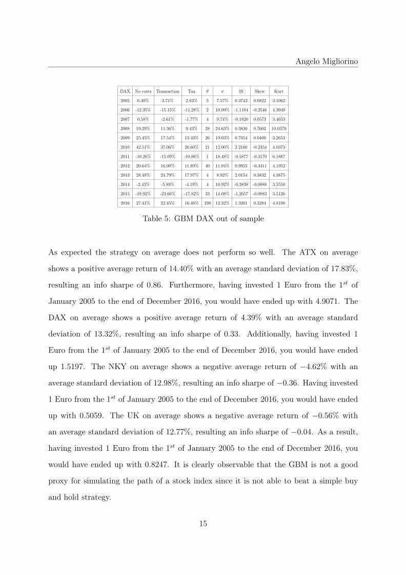
DAX No costs Transaction Tax θ σ IS Skew Kurt
2005 6.40% 3.71% 2.83% 5 7.57% 0.3743 0.0822 3.1062
2006 -12.35% -15.15% -11.28% 2 10.09% -1.1184 -0.2546 4.3949
2007 0.58% -2.61% -1.77% 4 9.74% -0.1820 0.0573 3.4653
2008 19.29% 11.36% 9.43% 28 24.63% 0.3830 0.7602 10.0379
2009 25.45% 17.54% 13.43% 26 19.03% 0.7054 0.0400 3.2653
2010 42.51% 37.06% 26.60% 21 12.00% 2.2160 -0.2354 4.0373
2011 -10.26% -15.09% -10.86% 1 18.48% -0.5877 -0.3170 6.1887
2012 20.64% 16.00% 11.89% 40 11.94% 0.9955 -0.3411 4.1952
2013 28.48% 24.79% 17.97% 4 8.92% 2.0154 0.3832 4.3875
2014 -2.43% -5.89% -4.19% 4 10.92% -0.3838 -0.0888 3.5550
2015 -19.92% -23.66% -17.82% 33 14.08% -1.2657 -0.0083 3.5126
2016 27.41% 22.45% 16.48% 198 12.32% 1.3381 0.3284 4.8198
Table 5: GBM DAX out of sample
As expected the strategy on average does not perform so well. The ATX on average
shows a positive average return of 14.40% with an average standard deviation of 17.83%,
resulting an info sharpe of 0.86. Furthermore, having invested 1 Euro from the 1st of
January 2005 to the end of December 2016, you would have ended up with 4.9071. The
DAX on average shows a positive average return of 4.39% with an average standard
deviation of 13.32%, resulting an info sharpe of 0.33. Additionally, having invested 1
Euro from the 1st of January 2005 to the end of December 2016, you would have ended
up 1.5197. The NKY on average shows a negative average return of −4.62% with an
average standard deviation of 12.98%, resulting an info sharpe of −0.36. Having invested
1 Euro from the 1st of January 2005 to the end of December 2016, you would have ended
up with 0.5059. The UK on average shows a negative average return of −0.56% with
an average standard deviation of 12.77%, resulting an info sharpe of −0.04. As a result,
having invested 1 Euro from the 1st of January 2005 to the end of December 2016, you
would have ended up with 0.8247. It is clearly observable that the GBM is not a good
proxy for simulating the path of a stock index since it is not able to beat a simple buy
and hold strategy.
15
Angelo Migliorino
6 Alternative Econometric Models
6.1 Methodology
Below it is explained a new model that tries to forecast indices prices. In order to forecast
future prices several steps are required.
Firstly, multiple rolling linear regressions have been run for open and close prices:
yt = α + β1x1 + β2x2 + ε
Where yt is a vector of prices of the index to be predicted that goes from t to t−δ. x1 and
x2 are the independent variables, meaning the two indices used to forecast the dependent
variable. In order to choose which indices should forecast the future price of the others
it has been computed a correlation table between all indices. The independent variable
chosen are the ones with the highest correlation with the dependent one.
Once it has been estimated the coefficients of the regressions, it is possible to forecast the
future prices (open and close):
yt+1 = α̂ + β̂1x1 + β̂2x2
Until now there is not something innovative. What is really innovative is the following.
After having estimated the futures open and closing prince, it has been computed the
hypothetical arithmetic return 13:
φ =ycloset+1
yopent+1
− 1
13In the long run it is better to use the arithmetic return instead of the logarithmic. This because thelog returns are an approximation given by the fact that ln(1 + r) ≈ r ⇐⇒ r is small.
16

Angelo Migliorino
From this point it is possible to implement two different strategies:
1. A simple strategy that do not involve using boundaries:
• if φ < 0 the strategy involves investing in a short position in the future;
• if φ > 0 the strategy involves investing in a long position in the future.
2. An aggressive strategy that uses some boundaries explained below:
• If φ < γ1 the strategy involves investing in two short positions in the future;
• if γ1 ≤ φ ≤ γ2 the strategy involves investing in one short position in the
future;
• if γ2 ≤ φ ≤ γ3 the strategy involves to not invest;
• if γ3 ≤ φ ≤ γ4 the strategy involves investing in one long position in the future;
• If φ > γ4 the strategy involves investing in two long positions in the future;
The most difficult part, now, is to set the time of the rolling regression and the boundaries
(γi with i = 1, 2, 3, 4). In order to estimate these coefficients, it has been imposed an
optimization problem given some constraint. The objective function to maximize is the
cumulative return that an investor would have get for the previous year following the
strategies. It is possible to define the two maximization problems as the following:
1.
max y = f(t)
2.
max y = f(t, γ1, γ2, γ3, γ4)
The constraints are the following:
17

Angelo Migliorino
• the variable t (time) is an integer constraint.
• γ1 ≤ γ2 ≤ γ3 ≤ γ4
• −2 ≤ γi ≤ 2, i = {1, 2, 3, 4}
6.2 Alternative model Results
We present below the results the simple and the aggressive strategies.
As for the GBM, the strategies have been implemented for four different stock indices.
6.2.1 Simple Strategy
Table 6 summarize the dependent and independent variable of the model.
Y X1 X2
Atx FtseMib Ibex
Dax S&P 500 Ccmp
Ftse100 S&P 500 Smi
Nikkei Aex Smi
Table 6: Resume indices
The Y is the index in which the investor should make operations. The independent vari-
able, instead, are the indices that one needs to forecast prices. In the tables 7, 8, 9 and
10, there are the statistical of the out of sample strategies of the first model.
18

Angelo Migliorino
NKY No costs Transaction Tax σ IS Skew Kurt Rolling period
2005 1.39% -1.32% -0.86% 13.26% -0.0650 0.2865 4.4380 25
2006 -15.98% -19.27% -14.43% 8.14% -1.7736 -0.0709 3.9627 9
2007 21.01% 17.14% 12.62% 12.38% 1.0188 -0.0370 2.9951 102
2008 148.14% 128.88% 87.13% 9.25% 9.4241 0.8634 7.4969 77
2009 138.67% 127.25% 84.27% 14.17% 5.9474 0.3627 3.6429 394
2010 37.95% 33.47% 24.03% 9.98% 2.4075 -0.1103 3.8101 397
2011 31.81% 27.81% 20.17% 10.20% 1.9779 -0.1457 3.7066 58
2012 -13.46% -15.75% -11.18% 11.73% -1.0064 2.6238 26.3132 53
2013 -35.36% -38.40% -29.82% 8.07% -3.6973 -0.1800 4.1947 24
2014 20.87% 17.09% 12.59% 15.32% 0.8216 -1.0202 9.2569 171
2015 -2.20% -5.46% -3.86% 9.74% -0.3964 -0.0132 3.9428 75
2016 26.13% 20.52% 15.35% 16.15% 0.9564 0.2886 5.9384 230
Table 7: S1 NKY out of sample
UK No costs Transaction Tax σ IS Skew Kurt Rolling period
2005 22.14% 19.45% 14.14% 8.10% 1.7466 0.0974 3.4731 69
2006 -5.59% -8.46% -6.19% 9.71% -0.6368 -0.1094 4.2839 322
2007 30.10% 24.70% 18.09% 8.23% 2.1990 0.1337 3.8816 267
2008 114.70% 97.38% 67.62% 11.47% 5.8937 0.0699 5.4828 59
2009 36.11% 28.58% 21.09% 27.96% 0.7543 0.7717 5.2505 98
2010 57.08% 50.61% 35.80% 13.45% 2.6618 -0.6163 4.9958 257
2011 64.40% 56.22% 39.71% 14.94% 2.6578 0.0747 4.1329 354
2012 12.91% 9.12% 6.88% 15.26% 0.4504 0.2437 3.5444 282
2013 -2.00% -4.93% -3.53% 10.33% -0.3414 -0.0560 3.4705 148
2014 -1.16% -3.78% -2.69% 6.85% -0.3929 -0.0512 3.4705 331
2015 44.06% 38.28% 27.47% 7.55% 3.6388 0.2831 4.3516 106
2016 23.62% 18.69% 13.84% 12.75% -0.0552 4.1190 1.0988 234
Table 8: S1 UK out of sample
19
Angelo Migliorino
ATX No costs Transaction Tax σ IS Skew Kurt Rolling period
2005 23.74% 19.57% 14.35% 10.26% 1.3988 0.3808 4.4468 21
2006 11.80% 6.52% 5.23% 15.45% 0.3384 -0.9555 8.9649 1
2007 45.59% 38.47% 27.74% 14.92% 1.8588 0.0722 8.969 71
2008 37.44% 22.93% 19.19% 35.63% 0.5386 -0.4292 4.7151 104
2009 35.77% 23.79% 18.59% 26.74% 0.6950 0.0910 3.2258 18
2010 55.82% 46.94% 33.72% 17.88% 1.8853 -0.9035 8.4845 148
2011 13.65% 5.96% 5.26% 21.91% 0.2402 -0.0450 4.4508 28
2012 27.85% 21.12% 15.77% 16.26% 0.9699 -0.2958 3.7610 7
2013 44.30% 38.62% 27.65% 11.86% 2.3319 0.2150 4.4456 1
2014 46.85% 40.85% 29.20% 12.32% 2.3690 -0.0066 3.7926 5
2015 12.02% 6.59% 5.25% 14.97% 0.3505 -0.0154 3.6791 49
2016 21.83% 15.62% 11.85% 16.03% 0.7390 -0.4842 5.2833 19
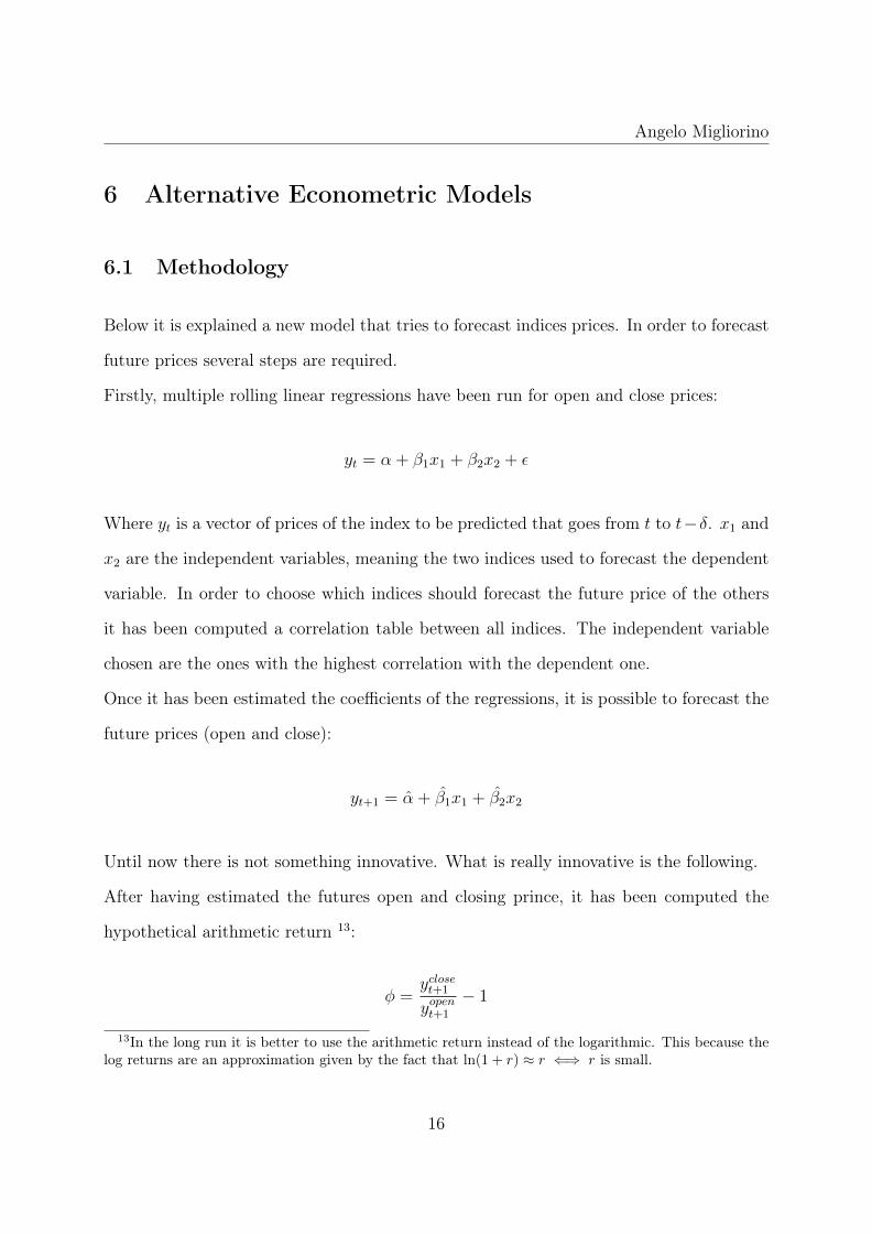
Table 9: S1 ATX out of sample
DAX No costs Transaction Tax σ IS Skew Kurt Rolling period
2005 -10.15% -12.42% -9.26% 7.58% –1.2212 -0.0308 3.1312 106
2006 -14.89% -17.61% -13.20% 10.12% -1.3044 -0.6069 4.2872 26
2007 9.19% 5.74% 4.39% 9.71% 0.4516 0.0545 3.4548 227
2008 0.38% -7.06% -4.22% 24.79% -0.1701 -0.7464 10.5419 81
2009 109.67% 96.51% 65.91% 18.77% 3.5119 -0.3894 3.6187 342
2010 -36.36% -38.83% -30.30% 12.06% -2.5119 -0.5609 3.5547 51
2011 1.66% -3.75% -2.21% 18.32% -0.1207 -0.0190 6.2697 1
2012 -0.23% -4.12% -2.81% 12.18% -0.2310 -0.1569 4.0901 5
2013 3.35% 0.37% 0.42% 9.04% 0.0463 -0.0877 4.5620 22
2014 10.82% 6.91% 5.29% 10.88% 0.4859 -0.0993 3.5954 4
2015 46.31% 39.52% 28.39% 13.93% 2.0378 0.1722 3.3805 58
2016 21.66% 16.94% 12.58% 12.52% 1.0050 0.3773 4.6659 55
Table 10: S1 DAX out of sample
The ATX on average shows a positive average return of 17.82% with an average standard
deviation of 18.10%, resulting an info sharpe of 0.98. Furthermore, having invested 1
Euro from the 1st of January 2005 to the end of December 2016, you would have ended
up with 6.8737. The DAX on average shows a positive average return of 4.58% with
an average standard deviation of 13.33%, resulting an info sharpe of 0.34. Furthermore,
having invested 1 Euro from the 1st of January 2005 to the end of December 2016, you
would have ended up with 1.3227. The NKY on average shows a positive average return
20

Angelo Migliorino
of 16.33% with an average standard deviation of 11.53%, resulting an info sharpe of 1.42.
Furthermore, having invested 1 Euro from the 1st of January 2005 to the end of December
2016, you would have ended up with 3.8217. The UK on average shows a positive average
return of 19.35% with an average standard deviation of 12.22%, resulting an info sharpe
of 1.58. Furthermore, having invested 1 Euro from the 1st of January 2005 to the end of
December 2016, you would have ended up with 7.0894. This strategy clearly outperform
the GBM results. It is interesting to notice that the info Sharpe are really high. The are
all above 1, only the DAX has a IS of 0.34 (not so efficient).
6.2.2 Aggressive Strategy
In the following tables 11, 12, 13 and 14 are shown the results of the second strategy for
the different indices.
UK No costs T.cos TT.cos σ IS Skew Kurt R. period γ1 γ2 γ3 γ4
2005 118.25% 108.96% 73.01% 12.32% 5.9283 0.3306 3.5176 342 -0.320% -0.297% -0.271% -0.240%
2006 30.92% 23.09% 17.35% 18.87% 0.9196 -0.4372 4.6337 371 -0.373% -0.371% -0.864% -0.606%
2007 39.63% 29.45% 22.32% 24.27% 0.9197 -0.3568 5.1272 302 -24.751% -5.612% -6.143% -0.622%
2008 305.22% 242.75% 162.36% 55.13% 2.9451 0.4168 6.3302 98 -8.036E-03% -8.093E-03% -7.666E-03% 8.549E-03%
2009 73.31% 54.90% 41.16% 34.42% 1.1958 0.0594 4.4341 261 -2.747E-03% -2.748E-03% -2.746E-03% 1.928E-03%
2010 161.20% 140.37% 93.62% 25.48% 3.6736 -0.4503 5.7595 284 -1.294 E-03% 1.496 E-06% 5.432E-05% 1.401E-02%
2011 158.42% 133.42% 90.48% 31.15% 2.9047 0.0688 4.1932 354 -1.183E-15% 3.656E-11% -2.647E-09% 7.708E-10%
2012 35.06% 26.14% 19.67% 20.92% 0.9402 -0.0737 3.5029 147 -3.470 E-10% -2.151E-11% 1.575E-11% -1.528E-11%
2013 -5.41% -11.00% -7.71% 18.27% -0.4221 -0.7589 4.5973 148 9.457E-10% -6.026E-10% -3.265E-07% -4.208-8%
2014 -3.57% -8.63% -5.99% 16.90% -0.3542 -0.5357 5.0141 331 9.144E-06% -3.277E-06% -8.143E-06% -5.033E-06%
2015 101.48% 85.68% 59.88% 25.31% 2.3655 0.1307 4.8281 106 0 0 0 0
2016 46.46% 35.05% 26.30% 25.14% 1.0461 -0.3166 4.3332 234 -1.809E-02% 5.393E-05% -3.053E-06% 7.209E-04%
Table 11: S2 UK out of sample
21
Angelo Migliorino
UK No costs T.cos TT.cos σ IS Skew Kurt R. period γ1 γ2 γ3 γ4
2005 1.67% -3.60% -2.23% 16.16% -0.1380 0.0788 4.1673 25 -0.01761% -0.00181% 0.00009% 0.01987%
2006 -28.20% -33.30% -25.22% 16.16% -1.1199 -0.0069 3.4763 9 -0.25770% -5.6246E-03% 9.0070E-03% 3.4171E-02%
2007 12.41% 5.34% 4.65% 20.03% 0.2322 0.55927 6.1420 55 0 0 0 0
2008 1433.04% 1211.04% 606.13% 54.26% 11.1701 1.3335 8.2106 203 -3.2499E-02 -3.2414E-02 -2.8354E-02 -1.9340E-02
2009 454.46% 402.72% 235.31% 28.45% 8.2697 0.3736 3.6334 396 0 0 0 0
2010 81.42% 69.95% 49.08% 19.67% 2.4950 -0.1044 3.9184 397 -3.0286E-07 -9.7535E-08 -7.7336E-08 2.8588E-08
2011 69.90% 59.80% 42.66% 22.50% 1.8962 2.9588 30.1696 58 0 0 0 0
2012 -25.42% -29.27% -22.25% 16.09% -1.3825 -0.3624 3.9189 53 -2.3270E-04 -1.0597E-04 -7.2119E-03 -4.3934E-03
2013 -60.05% -63.75% -51.96% 30.63% -1.6961 -1.2281 8.7871 24 0 0 0 0
2014 -8.16% -13.61% -9.63% 19.97% -0.4822 -1.2281 6.0790 128 -41.47% -23.37% -17.35% -1.38%
2015 -6.52% -12.66% -8.72% 22.23% -0.3923 -0.8701 9.3128 75 0 0 0 0
2016 46.41% 33.78% 26.41% 32.20% 0.8202 -1.2022 12.1614 251 -0.2651% -0.2587% -0.2408% -0.1929%
Table 12: S2 NKY out of sample
2005 55.78% 48.18% 34.29% 14.71% 2.3309 -0.2239 3.3459 199 -16.3459% -3.6993% -3.5054% -1.8618%
2006 11.98% 5.45% 4.69% 19.24% 0.2439 -0.5829 5.0758 333 -1.4586% -1.3891% -1.1336% -0.0875%
2007 63.33% 53.34% 38.10% 19.11% 1.9930 0.1949 3.4378 76 -0.1751% -0.1707% -0.1547% -0.1485%
2008 19.90% 4.44% 7.87% 49.34% 0.1595 0.0492 10.4652 103 -3.1183E-05 -3.1182E-05 -3.1189E-05 3.1194E-05
2009 48.41% 30.92% 25.14% 37.37% 0.6728 0.0492 3.5832 18 -3.3330E-02% -2.5139E-02% 0.1025% 0.1414%
2010 6.99% -1.10% 0.23% 24.36% 0.0093 -0.2326 3.8332 187 -1.5720% -1.5717% -1.5715% -1.5657%
2011 6.77% -4.31% -0.87% 36.68% -0.0237 -0.2147 6.2862 28 0 0 0 0
2012 32.53% 22.41% 17.36% 24.29% 0.7147 -0.1787 4.1204 148 –4.0127E-07% 4.0150E-07% 4.3526E-07% 6.1159E-07%
2013 7.65% 3.07% 2.62% 14.12% 0.1857 -0.1489 5.4261 42 -0.8301% -2.1104E-02% -3.3776E-03% 0.1661%
2014 -35.20% -39.71% -30.65% 21.74% -1.4097 0.0775 3.5936 9 0 0 0 0
2015 22.79% 11.63% 10.00% 28.14% 0.3555 -0.0418 3.4896 49 0 0 0 0
2016 14.67% 8.79% 7.05% 18.25% 0.3865 0.1664 6.65239 294 -0.5524% -0.2268% -1.1511E-02% -1.1208%
Table 13: S2 DAX out of sample
UK No costs T.cos TT.cos σ IS Skew Kurt R. period γ1 γ2 γ3 γ4
UK No costs T.cos TT.cos σ IS Skew Kurt R. period γ1 γ2 γ3 γ4
2005 158.07% 142.04% 93.60% 18.93% 4.9437 -0.1937 5.3461 98 -113.7989% -61.6739% -12.4074% -1.0590%
2006 96.12% 78.25% 55.98% 30.94% 1.8360 -0.8376 9.4889 38 -0.5975% -0.5615% -0.5255% -0.5194%
2007 130.03% 108.14% 74.74% 29.77% 2.5104 0.0220 4.7546 69 -0.1487% -0.1487% -0.1487% -0.1487%
2008 57.30% 25.64% 30.06% 71.25% 0.4219 -0.4387 5.7653 103 -2.6770E-03 -1.7822E-03 -1.2258E-03 2.7044E-03
2009 30.68% 8.94% 11.93% 52.93% 0.2254 0.0896 3.3384 18 0.1560% 0.1609% 0.2265% 0.2557%
2010 372.53% 324.27% 197.72% 33.91% 5.8312 -1.1100 10.6233 334 -1.1460% -0.8518% -0.6913% -0.6210%
2011 26.53% 2.85% 5.61% 43.81% 0.1282 -0.0450 4.4508 28 0 0 0 0
2012 26.53% 13.51% 16.39% 32.62% 0.3659 -0.4640 3.7768 148 5.1472E-08% -8.5844E-10% -6.1736E-08% 2.4762E-08%
2013 101.40% 85.86% 11.94% 23.75% 2.5173 -0.0095 4.5951 392 0 0 0 0
2014 49.34% 37.36% 27.87% 24.87% 1.1207 -0.1084 3.8164 9 0 0 0 0
2015 20.46% 9.05% 8.31% 29.94% 0.2777 -0.0154 3.6791 49 0 0 0 0
2016 39.82% 27.05% 21.32% 30.10% 0.7083 -0.5325 6.0876 264 -1.1570% -1.1417% -1.0637% -0.3988%
Table 14: S2 ATX out of sample
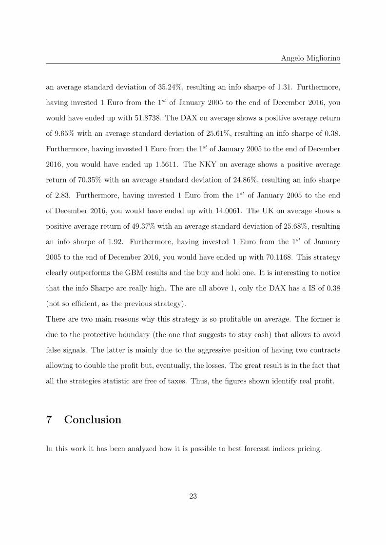
The overall average return are much higher comparing to the buy and hold, the GBM and
the simple strategy. The ATX on average shows a positive average return of 46.29% with
22
Angelo Migliorino
an average standard deviation of 35.24%, resulting an info sharpe of 1.31. Furthermore,
having invested 1 Euro from the 1st of January 2005 to the end of December 2016, you
would have ended up with 51.8738. The DAX on average shows a positive average return
of 9.65% with an average standard deviation of 25.61%, resulting an info sharpe of 0.38.
Furthermore, having invested 1 Euro from the 1st of January 2005 to the end of December
2016, you would have ended up 1.5611. The NKY on average shows a positive average
return of 70.35% with an average standard deviation of 24.86%, resulting an info sharpe
of 2.83. Furthermore, having invested 1 Euro from the 1st of January 2005 to the end
of December 2016, you would have ended up with 14.0061. The UK on average shows a
positive average return of 49.37% with an average standard deviation of 25.68%, resulting
an info sharpe of 1.92. Furthermore, having invested 1 Euro from the 1st of January
2005 to the end of December 2016, you would have ended up with 70.1168. This strategy
clearly outperforms the GBM results and the buy and hold one. It is interesting to notice
that the info Sharpe are really high. The are all above 1, only the DAX has a IS of 0.38
(not so efficient, as the previous strategy).
There are two main reasons why this strategy is so profitable on average. The former is
due to the protective boundary (the one that suggests to stay cash) that allows to avoid
false signals. The latter is mainly due to the aggressive position of having two contracts
allowing to double the profit but, eventually, the losses. The great result is in the fact that
all the strategies statistic are free of taxes. Thus, the figures shown identify real profit.
7 Conclusion
In this work it has been analyzed how it is possible to best forecast indices pricing.
23

Angelo Migliorino
The Geometric Brownian motion is supposed to be a good proxy for simulating the path
of stock indices but of course has a lot of bias inside, mostly given by the parameters
estimated in the model. This results to have a poor average performance for the four
indices taken in analysis. The Austrian index shows on average an IS of 0.86, the England
index figures on average a IS -0.04, the Japanese index a negative average IS of -0.36 and
the German index a positive average IS of 0.33.
The simple alternative strategy performs really well on average, much better than the
GBM and the buy and hold. The Austrian index shows on average an IS of 0.98, the
England index figures on average a IS 1.58, the Japanese index an average IS of 1.42 and
the German index a positive average IS of 0.34.
The aggressive alternative strategy performs really well on average, much better than the
GBM, the simple model and the buy and hold. The Austrian index shows on average an
IS of 1.31, the England index figures on average a IS 1.92, the Japanese index an average
IS of 2.83 and the German index a positive average IS of 0.38. This can be achieved
thanks to the protective boundary that allows to stay cash and avoid false signal and the
aggressive boundaries.
Further improvements can be done studying different indices and constructing equally
weighted or risk parity portfolios. Diversifying on different indices can allow to avoid
single shock on specific countries. Furthermore, including more independent variables
may improve the forecast power, allowing to increase more the profit.
24
Angelo Migliorino
ReferencesAng, A. (2014). Asset Management: A Systematic Approach to Factor Investing. Oxford Uni-
versity Press.
Berk, J. and DeMarzo, P. (2007). Corporate finance. Pearson Education.
Black, F. (1993). Beta and return. journal of portfolio management, 20:8–18.
Bodie, Z., Kane, A., and Marcus, J. A. (2014). Investments, 10e. McGraw-Hill Education.
Brockwell, J. P. and Davis, R. A. (2016). Introduction to time series and forecasting. springer.
Cahart, M. M. (1997). On persistence in mutual fund performance. The Journal of finance 52,1:57–82.
Campbell, Y. J., Lo, A. W. C., and MacKinlay, A. C. (1997). The Econometrics Of FinancialMarkets. Princeton University press.
Daniotti, E. (2012). Is technical analysis able to beat market inefficiency? In Mathematical andStatistical Methods for Actuarial Sciences and Finance, 1:165–173.
Ericsson, J. and Karlsson, S. (2004). Choosing factors in a multifactor asset pricing model: Abayesian approach. SSE/EFI Working Paper Series in Economics and Finance, 524.
Fama, E. F. (1969). Efficient capital markets: A review of theory and empirical work. TheJournal of Finance, 25(2).
Fama, E. F. and French, K. R. (1993). Common risk factors in the returns on stocks and bonds.Journal of financial economics, 33(1):3–56.
Fama, E. F. and French, K. R. (2014). A five-factor asset pricing model. Journal of FinancialEconomics.
Kim, H. and Han, S. T. (2016). The enhanced classification for the stock index prediction.Procedia Computer Science, 91:284–286.
Menkhoff, L. and Taylor, M. P. (2007). The obstinate passion of foreign exchange professionals:Technical analysis? Journal of Economic Literature, 45(4):936–972.
Murphy, J. J. (1999). Technical analysis of the financial markets: A comprehensive guide totrading methods and applications. New York Institute of Finance.
Ross, S. M. (2014). Introduction to Probability Models. Academic press.
Sonono, M. E. and Mashele, H. P. (2015). Prediction of stock price movement using continuoustime models. Journal of Mathematical Finance, 5:178–191.
Stirzaker, D. (2005). Stochastic Processes and Models. Oxford University Press.
25