novel cheminformatics methods for modeling biomolecular

Novel Cheminformatics Methods for Modeling Biomolecular Data in High

Dimension Low Sample Size (HDLSS) Chemistry Space

Tong-Ying Wu

A dissertation submitted to the faculty of the University of North Carolina at Chapel Hill

in partial fulfillment of the requirements for the degree of Doctor of Philosophy in the

Department of Biomedical Engineering.

Chapel Hill

2011

Approved By:

Alexander Tropsha, Ph.D.

David Lalush, Ph.D.

J. S. Marron, Ph.D.

Jack Snoeyink, Ph.D.

Shawn Gomez, Ph.D.

ii

© 2011

Tong-Ying Wu

ALL RIGHTS RESERVED

iii

ABSTRACT

TONG-YING WU: Novel Cheminformatics Methods for Modeling Biomolecular Data in

High Dimension Low Sample Size (HDLSS) Chemistry Space

(Under the direction of Dr. Alexander Tropsha)

The increasing availability of biological and chemical data has led to a critical need for

cheminformatics and bioinformatics tools to analyze the data. However, not all datasets contain

sufficient information for significant analysis. One problem is High Dimension Low Sample Size

(HDLSS), where the number of structural characteristics, e.g., molecular descriptors, that can be

calculated from a single compound (high dimensionality) far exceeds the number of compounds

(low sample size). A major challenge associated with modeling HDLSS data is overfitting, and

specialized tools are required to overcome the statistical difficulties inherent to HDLSS. We

improved the Distance Weighted Discrimination (DWD) statistical learning method through a

new variable selection technique for estimating the intrinsic dimension of a dataset, i.e., the

minimum number of descriptors to classify data. Compared to SVM and DWD without variable

selection, DWD with variable selection achieved higher prediction accuracy on several

benchmarking datasets and allowed the identification of key molecular features that contribute to

investigated biological properties, e.g., inhibition of AmpC β-lactamase and binding affinity for

the various serotonin receptors.

For analyzing and modeling stereochemistry-dependent datasets, we developed chiral

atom-pair descriptors (3D chiral atom-pair), which were calculated from three-dimensional

molecular structures. QSAR models built with these descriptors, versus either 3D non-chiral

atom-pair or 2D Dragon descriptors, more accurately predicted antimalarial activity and binding

iv

affinities of small molecules toward various receptors. Our method not only led to the

identification of a subset of chiral atoms that are expected to affect the selected biological

property, e.g., antimalarial activity, but also enabled the development of models that would not be

possible otherwise.

To aid automatic protein function annotation, especially in the case of functional

homologs, we developed new protein descriptors based solely on protein's structure. Our method

showed sensitivity comparable to that of ScanPROSITE. When predicted annotations from both

ScanPROSITE and our method were combined into a consensus model, we observed a significant

gain in prediction reliability and the successful functional annotation of proteins with low

sequence similarity.

v

Dedication

To my family for their continuous support in overcoming the difficulties in life. To my

grandmother, who passed away prior to my pursuit of a Ph.D. degree, for always believing in me.

My love for her and sadness at her passing have fueled my determination to be an active member

in the medical and pharmaceutical research rather than just bring the life saving technologies to

people.

vi

Acknowledgments

Numerous people contributed to the research projects described in this dissertation, and I

am grateful to all of them for their discussion and support. I would like to acknowledge my

research chair, Dr. Alexander Tropsha, for his supervision, guidance, and funding that made this

research possible. This research could not have been completed without Dr. J.S. Marron’s

expertise in Object Oriented Data Analysis, especially for HDLSS data. Dr. Jack Snoeyink’s

expertise in computational geometry and Dr. Shawn Gomez’s suggestions on protein function

annotation facilitated the study of the protein structure-function relationship. In order to study the

contribution of stereochemistry in biological activities, Dr. Weifan Zheng’s guidance in chirality

descriptors was critical. I also like to express my gratitude to m committee chair, Dr. David

Lalush, and the Director in Graduate Studies in BME, Dr. Paul Dayton, for their effort to resolve

the challenges that I faced during my study. I also would like to thank Dr. Denis Fourches, Dr.

Eugene Muratov, Dr. Alexander Sedykh, Dr. Alexander Golbraikh and Mr. Stephen J. Bush for

their feedback and criticisms for improving this manuscript. Discussions with Dr. Wei Wang, Dr.

Leonard McMillan, Dr. Jan Prins, Dr. Brian Kuhlman, Dr. Tim Elston, and Dr. Yufeng Liu also

made impacts on this research.

Additionally, I owe my deepest gratitude to the following people for their guidance in

computer-aided drug design: Dr. Markus Boehm and Dr. Gregory A. Bakken from Pfizer for their

knowledge in lead identification; Dr. Christian Lemmen, Dr. Holger Claussen, and Dr. Markus

Lilienthal from Bio SolveIT for their help to implement an efficient similarity search method in

large databases; Dr. Chris Bizon from Renaissance Computing Institute and Dr. Dana E.

Vanderwall from Bristol-Myers Squibb for their knowledge in multi-property lead optimization;

vii

Dr. Martha S. Head, Dr. Kaushik Raha, Dr. Deepak Bandyopadhyay from GlaxoSmithKline

(GSK) for their knowledge in the structure-based drug design and the identification of the protein

binding sites; Dr. Daniel J. Price and Dr. Eugene L. Stewart from GSK and Dr. Zheng P. Yang

from Boehringer Ingelheim for their knowledge in the overall computer-aided drug design.

viii

Table of Contents

List of Tables ............................................................................................................................. xi

List of Figures ........................................................................................................................... xii

List of Abbreviations ................................................................................................................ xiv

Chapter 1 .................................................................................................................................... 1

Introduction ................................................................................................................................ 1

1.1 Background Information .............................................................................................. 1

1.1.1 Growth of Publically Available Data ........................................................................... 1

1.1.2 Overview of Computational Methods Employed in Drug Discovery ............................ 2

1.1.3 Applications of Classification Methods in Cheminformatics and Bioinformatics ......... 3

1.2 Research Motivation .......................................................................................................... 5

Chapter 2 .................................................................................................................................... 7

Variable Selection Based Classification Method for Imbalanced and HDLSS Data ...................... 7

2.1 Motivation ......................................................................................................................... 7

2.2 Overview of Variable Selection ......................................................................................... 9

2.3 Overview of the Proposed Method ................................................................................... 10

2.3.1 Variable Evaluation Component ................................................................................ 11

2.3.2 Variable Selection (Ranking) Component.................................................................. 12

2.5 Simulation ....................................................................................................................... 13

2.5.1 Experimental Design ................................................................................................. 13

2.5.2 Simulation Result...................................................................................................... 14

2.6 QSAR Studies ................................................................................................................. 18

2.7 QSAR Datasets Description ............................................................................................. 19

2.7.1 AmpC β–lactamases Dataset Description (110 Compounds) ...................................... 19

2.7.2 5-HT Datasets Description ........................................................................................ 20

2.8 QSAR Modeling Results.................................................................................................. 21

2.8.1 AmpC Β-lactamase Modeling Result (110 Compounds) ............................................ 21

ix

2.8.2 5-HT1B Modeling Result ........................................................................................... 24

2.8.3 5-HT1D Modeling Result ........................................................................................... 28

2.8.4 5-HT2B Modeling Result ........................................................................................... 32

2.8.5 5-HT6 Modeling Result ............................................................................................. 34

2.9 Conclusion ...................................................................................................................... 36

Chapter 3 .................................................................................................................................. 37

Novel Three-Dimensional Chirality Atom-Pair Descriptors ....................................................... 37

3.1 Motivation / Background ................................................................................................. 37

3.2 Overview of Current Chirality Descriptors ....................................................................... 40

3.2.1 Prior Implementation of the Chirality Descriptors ..................................................... 41

3.2.2 Three Dimensional Chiral Atom-Pair Descriptors...................................................... 42

3.3 Dataset Description.......................................................................................................... 45

3.3.1 Peptide Transporter 1 (PEPT1) Dataset ..................................................................... 45

3.3.2 AmpC β–lactamases Dataset (149 Compounds) ........................................................ 47

3.3.3 Artemisinin Dataset .................................................................................................. 49

3.4 Evaluation of Descriptor Significance and Generalizability .............................................. 50

3.5 Modeling Results ............................................................................................................. 51

3.5.1 PEPT1 Dataset .......................................................................................................... 51

3.5.2 AmpC β–lactamase Dataset (149 Compounds) .......................................................... 54

3.5.3 Artemisinin Dataset .................................................................................................. 56

3.6 Conclusion ...................................................................................................................... 59

Chapter 4 .................................................................................................................................. 61

Novel Protein Descriptors ......................................................................................................... 61

4.1 Growth of Protein Structure Data ..................................................................................... 61

4.2 Overview of Current Methods for Protein Function Annotation........................................ 64

4.2.1 Sequence-Based Methods ......................................................................................... 64

4.2.2 Structure-Based Methods .......................................................................................... 65

4.3 Motivation ....................................................................................................................... 68

4.4 Novel Protein Descriptors ................................................................................................ 68

4.4.1 Classification Scheme of Amino Acids (Ten Classes) and Geometric Properties ........ 69

4.4.2 Geometric Property of α–helix vs. β sheet ................................................................. 72

4.5 Selection of Enzyme Diversity Set ................................................................................... 75

x

4.6 Selection of Enzyme Homologs ....................................................................................... 76

4.6.1 Superoxide Dismutase (EC 1.15.1.1) ......................................................................... 77

4.6.2 Cellulase (EC 3.2.1.4) ............................................................................................... 78

4.6.3 β-lactamase (EC 3.5.2.6) ........................................................................................... 79

4.6.4 Methyltransferases (EC 2.1.1) ................................................................................... 80

4.6.5 Protein-Tyrosine Kinases (EC 2.7.10) ....................................................................... 81

4.6.6 Protein-Serine/Threonine Kinases (EC 2.7.11) .......................................................... 82

4.7 Modeling Results ............................................................................................................. 84

4.7.1 Superoxide Dismutase (EC 1.15.1.1) ......................................................................... 84

4.7.2 Cellulase (EC 3.2.1.4) ............................................................................................... 89

4.7.3 β-lactamase (EC 3.5.2.6) ........................................................................................... 92

4.7.4 Methyltransferases (EC 2.1.1) ................................................................................... 96

4.7.5 Protein-Tyrosine Kinases (EC 2.7.10) ....................................................................... 97

4.7.6 Protein-Serine/Threonine Kinase (EC 2.7.11) ............................................................ 98

4.8 Evaluating the Stability of the Delaunay Simplices .......................................................... 99

4.9 Comparison with PROSITE ........................................................................................... 102

4.9.1 Test Set Selection Criteria for Both E.C. 1.15.1.1 and E.C. 3.5.2.6 .......................... 102

4.9.2 Comparison Results ................................................................................................ 103

4.10 Conclusion .................................................................................................................. 105

Chapter 5 ................................................................................................................................ 108

Summary ................................................................................................................................ 108

xi

List of Tables

Table 2. 1. 5-HT receptor families and subtypes. ....................................................................... 20

Table 2. 2. The 49 unique descriptors selected by all 5 models. .................................................. 22

Table 2. 3. The unique descriptors selected by all 5 models from each of the three clusters. ....... 27

Table 2. 4. The unique descriptors selected by all 5 models from each of the three clusters. ....... 31

Table 2. 5. The 79 unique descriptors selected by all 5 models for the 5-HT2B dataset. ............... 33

Table 2. 6. The 87 unique descriptors selected by all 5 models for the 5-HT6 dataset. ................. 35

Table 3. 1. List of top ten single enantiomer blocker drugs in ranking order. .............................. 39

Table 3. 2. The 17 atom types defined in the atom pair descriptors............................................. 41

Table 4. 1. Possible categories of tetrahedra............................................................................... 70

Table 4. 2. Classification of amino acids. .................................................................................. 71

Table 4. 3. Fourteen PDB entries retrieved based on the selection criteria from EC 1.15.1.1....... 77

Table 4. 4. Eighteen PDB entries retrieved based on the selection criteria for EC 3.2.1.4. .......... 78

Table 4. 5. Twelve PDB entries retrieved based on the selection criteria for EC 3.5.2.6.............. 79

Table 4. 6. Thirty-two PDB entries retrieved based on the selection criteria for EC 2.1.1. .......... 80

Table 4. 7. Eleven PDB entries retrieved base on the selection criteria for EC 2.7.10. ................ 81

Table 4. 8. List of subfamilies associated with EC 2.7.11. .......................................................... 82

Table 4. 9. Twenty-two PDB entries retrieved based on the selection criteria for EC 2.7.11. ...... 83

Table 4. 10. The list of PDB entries selected for the two positive classes. ................................ 103

xii

List of Figures

Figure 2. 1. Informative descriptor vs. noise. ............................................................................. 13

Figure 2. 2. Prediction results of the 30 simulation runs. ............................................................ 15

Figure 2. 3. Identification of the optimal model through the z-score. .......................................... 16

Figure 2. 4. Model analysis of the simulated data. ...................................................................... 17

Figure 2. 5. Performance comparison between the methods (AmpC dataset). ............................. 21

Figure 2. 6. Common structure features of the AmpC inhibitors. ................................................ 23

Figure 2. 7. Dendrogram of the 5-HT1B dataset. ......................................................................... 24

Figure 2. 8. Data distribution of the 5-HT1B dataset in Dragon chemical descriptor space. .......... 25

Figure 2. 9. Performance comparison through five-fold external cross validation for the

5-HT1B dataset......................................................................................................... 26

Figure 2. 10. Dendrogram of the 5-HT1D dataset. ....................................................................... 28

Figure 2. 11. Data distribution of the 5-HT1D dataset in Dragon chemical descriptor space. ........ 29


5-HT1D dataset. ..................................................................................................... 30


5-HT2B dataset. ...................................................................................................... 32


5-HT6 dataset. ....................................................................................................... 34

Figure 3. 1. Two enantiomers of a generic amino acid. .............................................................. 37

Figure 3. 2. Growing trend of chiral technology. ........................................................................ 38

Figure 3. 3. Activity distribution of the PEPT1 binding substrates.............................................. 46

Figure 3. 4. Isoindole-like scaffold (top) vs. isoindole (bottom). ................................................ 47

Figure 3. 5. The two enantiomeric pairs observed in the additional AmpC dataset. ..................... 48

Figure 3. 6. Structure of artemisinin........................................................................................... 49

Figure 3. 7. Degrees of chirality and the corresponding significance for the PEPT1 dataset. ....... 51

Figure 3. 8. Five-fold external cross-validation results of the PEPT1 dataset. ............................. 53

Figure 3. 9. Degrees of chirality and the corresponding significance for AmpC

β-lactamase dataset (149 compounds)...................................................................... 54

Figure 3. 10. Five-fold external cross-validation result of AmpC β-lactamase dataset

(149 compounds). ................................................................................................. 55

Figure 3. 11. Degrees of chirality and corresponding significance for the artemisinin dataset. .... 57

Figure 3. 12. Five-fold external cross-validation result of the artemisinin dataset. ...................... 58

Figure 4. 1. Annual growth of structures in Protein Data Bank (PDB). ....................................... 62

Figure 4. 2. Annual growth of protein structures with unknown function. .................................. 63

Figure 4. 3. Illustration of the potential benefit by encoding the geometric property of

tetrahedra for proteins. ............................................................................................ 72

Figure 4. 4. α–helix vs. β–sheet. ................................................................................................ 73

Figure 4. 5. Difference in geometric properties of tetrahedra between α-helix and β sheet. ......... 74

xiii

Figure 4. 6. Distribution of the six major enzyme groups in the enzyme diversity set. ................ 75

Figure 4. 7. Identifying the most significant model through z-scores for the EC1.15.1.1

dataset. .................................................................................................................... 84

Figure 4. 8. The five most significant features associated with SOD. ......................................... 85

Figure 4. 9. Mapping the four identified tetrahedral categories onto structures associated

with SOD binding to Fe3+

and Mn2+

. ........................................................................ 86


with SOD binding to Cu2+

/Zn2+

and Ni2+

. ............................................................... 87

Figure 4. 11. Mapping the four identified tetrahedral categories onto PDB entry, 1TO4. ............ 88

Figure 4. 12. Identifying the most significant model through z-score for the EC 3.2.1.4

dataset. .................................................................................................................. 89

Figure 4. 13. The twenty most significant features associated with cellulase. ............................. 90

Figure 4. 14. Mapping the 18 identified tetrahedral categories on to the structures

associated with cellulases. ..................................................................................... 91

Figure 4. 15. Identifying the most significant model through z-score for the EC 3.5.2.6

dataset. .................................................................................................................. 92

Figure 4. 16. The ten most significant features associated with β-lactamase. .............................. 93

Figure 4. 17. Mapping the six identified tetrahedral categories on to the 1M2X and

1NYM structure entries (EC 3.5.2.6 family). ......................................................... 94

Figure 4. 18. Mapping the six identified tetrahedral categories on to the 3G35 structure

entry (EC 3.5.2.6 family). ...................................................................................... 95

Figure 4. 19. Identifying the most significant model through z-score for the EC 2.1.1

dataset. .................................................................................................................. 96

Figure 4. 20. Identifying the most significant model through z-score for the EC 2.7.10

dataset. .................................................................................................................. 97

Figure 4. 21. Identifying the most significant model through z-scores for the EC 2.7.11

dataset. .................................................................................................................. 98

Figure 4. 22. Mapping the four categories of tetrahedron found in the modified structures

onto the original 1TO4 PDB structure. ................................................................ 100

Figure 4. 23. Benchmarking results. ........................................................................................ 104

xiv

List of Abbreviations

2D Two-Dimensional

3D Three-Dimensional

5-HT 5-hydroxytryptamine

Ala Alanine

APair Regular Atom-pair (without chiral atom types)

Arg Arginine

Asn Asparagine

Asp Aspartic Acid

BCC Bond-charge Corrections

BLAST Basic Local Alignment Search Tool

Ca2+

Calcium (II) Cation

CADD Computer-aided Drug Design

CAMD Computer-aided Molecular Design

cAMP Cyclic Adenosine Monophosphate

cAP Chiral Atom-pair

CCR Correct Classification Rate

CDD Collaborative Drug Discovery

cGMP Cyclic Guanosine Monophosphate

Cu Cupper

Cu2+

Copper (II) Cation; Cupric Cation

Cys Cysteine

DNA Deoxyribonucleic Acid

DWD Distance Weighted Discrimination; weighted Distance

Weighted Discrimination DWD (No V.S.) wDWD without Variable Selection

DWD (V.S.)

DWD_VS

wDWD with Variable Selection

wDWD with Variable Selection

E.C. Enzyme Classification or Enzyme Commission

ET Evolutionary Trace

FDA US Food and Drug Administration

Fe Iron

Fe3+

Iron (III) Cation; Ferric Cation

Gln Glutamine

Glu Glutamate

Gly Glycine

GPSS Global Protein Surface Survey

HDLSS High Dimension Low Sample Size

His Histidine

HMM Hidden Markov Model

Ile Isoleucine

Leu Leucine

xv

Lys Lysine

Met Methionine

Mn Manganese

Mn2+

Manganese Cation

MSA Multiple Sequence Alignment

Ni

Ni2+

Nickel

Nickel(II) Cation; Nickelous Cation NMR Nuclear Magnetic Resonance

PCA Principal Component Analysis

PDB Protein Data Bank

PDSP Psychoactive Drug Screening Program

PEPT1 Peptide Transporter 1

Phe Phenylalanine

PINTS Patterns in Non-homologous Tertiary Structures

Pro Proline

PSI-BLAST Position-Specific Iterative BLAST

pvSOAR Pocket and Void Surfaces of Amino Acid Residues

QSAR Quantitative Structure-Activity Relationship

RA Relative Activity

RMS Root Mean Square

RMSD Root-mean-square Deviation

RNA Ribonucleic Acid

SCOP Structural Classification of Proteins

Ser Serine

SOD Superoxide Dismutase

SVM Support Vector Machine

Thr Threonine

Trp Tryptophan

Tyr Tyrosine

V.S. Variable Selection

Val Valine

wDWD weighted Distance Weighted Discrimination

Zn Zinc

Zn2+

Zinc Cation

Chapter 1

Introduction

1.1 Background Information

1.1.1 Growth of Publically Available Data

Due to technological advancements within the past two decades, rapid synthesis and

high-throughput screening of large chemical libraries have become routine procedures in the

pharmaceutical industry, which has resulted in a massive increase of data for chemical

compounds, and their targets, pathways, and associated data. These data were largely proprietary

and therefore rarely available to the academic research community. However, within the past

decade, high-throughput screening has become increasingly common in academia, and the

resulting data are typically published and often made publically available in relevant databases.

Additionally, some pharmaceutical companies are also beginning to put some of their datasets in

the public domain.

Several publically available databases have been created. PubChem 97

is a public database

that launched as a result of the cheminformatics initiatives from the National Institutes of Health

(NIH) in October, 2004. It contains data regarding chemical molecules whose activities have been

experimentally measured using biological assays. As of mid January, 2011, PubChem provides

open access to data from over 31 million pure and characterized chemical compounds and close

to 75 million substance mixtures, extracts, complexes, and other uncharacterized substances. Two

other public databases, PDSP 112

and ChEMBL 142

, are popular within the cheminformatics

community. PDSP currently contains 55,440 competitive inhibition assay data for psychoactive

2

compounds, and ChEMBL includes 8,372 targets, 1,000,470 distinct compounds, and 4,668,202

activities.

In 2010, after seeing the potential of open innovation, GlaxoSmithKline publically

released 13,471 molecules that had been screened for activity against malaria. This move marks

the first large-scale public release of experimentally tested chemical compounds by a

pharmaceutical company. These compounds and their associated screening data are available via

CDD (Collaborative Drug Discovery) Public 40

. As of January, 2011, CCD Public contains 69

datasets for a total of about 1.5 million small molecules 40

.

In addition to small-molecule databases, many public databases provide access to larger

biological molecules. For instance, Protein Data Bank (PDB) is a repository for the three-

dimensional x-ray crystallography or NMR spectroscopy data of large biological molecules such

as proteins and nucleic acids. As of January 13, 2011, the PDB contains 70,494 protein structure

entries.

1.1.2 Overview of Computational Methods Employed in Drug Discovery

Cheminformatics and bioinformatics tools, such as statistical classification methods, have

proven to be reliable in handling and analyzing large datasets 16

. However, the explosion of

publicly available biological and chemical data has lead to a critical need for modifications of

existing and developments of new cheminformatics and bioinformatics tools for integration of the

data 101

. These publicly available data could serve as a platform for computer-aided drug design

(CADD) that refers to discovery of new molecules with desirable properties through

computational methodologies. There are two major types of methods utilized in CADD:

structure-based and ligand-based. Structure-based methods utilize knowledge of the three

dimensional structure of a biological target (e.g., protein). However, many targets lack

experimental structures, in which case, a homology model based on the experimental structure

3

from a related protein may be used. Even worse, in many cases the biological target associated

with a disorder is unknown, and structure-based drug design cannot be used.

On the other hand, ligand-based methods do not require three-dimensional structural

information of biological targets. Instead, ligand-based methods, which are also referred to as

ligand-based drug designs (LBDD), only require one or more chemical compounds that display a

particular experimentally measured activity, thus allowing a broader range of applicability than

its structure-based counterpart. More specifically, LBDD identifies the structural characteristics

for a molecular compound, usually referred to as descriptors. These descriptors describe the

multi-dimensional features of a compound, e.g., molecular weight, topolology, volume, and are in

turn applied to estimate biological activity.

The assumption in LBDD is that structurally similar compounds will possess similar

biological activity. This structural similarity can be assessed either globally or locally using

descriptors. A global similarity search can work with only a single active compound, making it

especially useful in earlier phases of CADD where one does not have enough information about

the biological targets and few binding ligands are available. However, if only one active

compound is used, a global similarity search will utilize all descriptors, including those irrelevant

to the biological activity of interest. In contrast, local similarity search methods can identify

molecular descriptors relevant to the biological activity, but they also require more compounds

known to have the requested biological activity. Because more and more experimental screening

data are being made available, LBDD using local similarity is becoming increasingly applicable.

1.1.3 Applications of Classification Methods in Cheminformatics and Bioinformatics

Biological activities can be generalized into two types: continuous and categorical. For

modeling categorical data, there are two learning methods to group data: unsupervised and

supervised. In unsupervised learning (referred to as cluster analysis), the problem is to analyze a

single dataset and decide how and whether the observations in the dataset can be divided into

4

groups. Supervised learning (referred to as classification) is a method of assigning unknown

entities into known groups. The goal is to learn from training sets and then apply the knowledge

to test sets. Thus, entities from test sets are placed into established groups, i.e., active or inactive,

based on their measurable quantitative characteristics. Although both classification and cluster

analysis determine which group a compound belongs to based on the quantitative measurements,

the sorting of groups associated with classification attempts to identify the contributions of the

quantitative measures to the established groups. In fact, classification, as a method for

information extraction, has been applied to many fields, including cheminformatics and

bioinformatics, which are important in the drug discovery process.

In bioinformatics, classification is applied from microarray gene expression data to

proteins. In gene expression analysis, the goal is to separate signal from noise in high-throughput

gene expression studies. Another important application of classification in bioinformatics is

classifying proteins into groups. The grouping, which is well established, can be based on the

similarities in structures or functions of proteins. The functional grouping of proteins can be

found by the Enzyme Classification (EC) number while Structural Classification of Proteins

(SCOP) provides the structural grouping of proteins. Given a group of proteins, the goal of

classification is to identify common patterns (or motifs) that are conserved.

In cheminformatics, quantitative structure-activity relationship (QSAR) modeling relies

on machine learning methods to correlate molecular descriptors to well-defined biological

activities, which can be categorized into groups, such as inhibitors, weak inhibitors, and non-

inhibitors. In the scenario of categorized biological activity, classification is used to build models

from the molecules in the training set and then to predict the biological activities of unknown

molecules through these models. These models select molecular descriptors that are relevant to

the biological activity from a population of descriptors determined either empirically or by

computational methods. Selected descriptors, which encode structural or property parameters,

provide clues to understanding the structural requirements for compounds to exhibit biological

5

activity. With the amount of biomolecular data available to the public, classification is ideal to

analyze these data and to identify important molecular features attributing to the given biological

activity.

1.2 Research Motivation

Modern QSAR studies are characterized by the use of multiple descriptors of chemical

structure combined with linear or non-linear machine learning methods in an attempt to build

predictive QSAR models through rigorous model validation. As summarized by Tropsha et al 136

,

the major differences between various QSAR paradigms are due to the different molecular

descriptors and the algorithms used to establish a correlation between descriptor values and

biological activity; however, there appears to be no universal QSAR paradigm that produces the

best QSAR models for any datasets. The combination of the significant increase in publicly

available datasets of biologically active compounds and the critical need to improve the hit rate of

experimental compound screening has created a strong need to develop reliable computational

QSAR modeling techniques and specific end-point predictors, i.e. a specific set of variables

expected to predict a biological activity (end-point).

The challenges associated with modeling these biomolecular data include (1) high

dimension low sample size (HDLSS), i.e., when the embedded dimension (e.g., number of

descriptors) far exceeds the sample size (e.g., number of molecules in the dataset), and (2)

imbalanced categorical data, i.e., when the number of samples in one class far exceeds that of the

other. HDLSS data is challenging largely due to the high likelihood of overfitting. Overfitting

occurs when a statistical model captures noise bias toward the training set instead of identifying

specific end-point predictors that describe the underlying biological activity relationship. Thus,

overfitting generally lowers the prediction accuracy for samples that are not part of the training

set.

6

Another challenge associated with modeling the biomolecular data is the imbalanced

class distribution of categorized biological activity, which means that there is at least one class of

instances which significantly outnumbers other classes. This challenge is also referred in this

dissertation as the imbalanced categorical characteristic. Some modern classification methods,

which optimize the overall misclassification rate of the whole training set, do not perform well on

data with imbalanced categorical characteristic, because such methods generally assume a

relatively balanced class distribution and put too much strength on the majority class.

There is a middle ground between using simplistic models that are traditional in

biochemistry and letting powerful computers free to do data mining on a huge number of

potential features. In this dissertation, we demonstrate the benefit of choosing models that

attempt to capture a (relatively) small number of chosen features that are then subjected to

statistical analysis. Specifically, we show that

(i) estimating the intrinsic dimension of a dataset can improve DWD statistical learning,

and overcome the statistical difficulties inherent to biological data with high dimension, low

sample size (HDLSS) and imbalanced categorical characteristics;

(ii) novel, three-dimensional chiral atom-pair descriptors for stereochemistry-dependent

datasets produce more accurate QSAR models; and

(iii) new protein descriptors based solely on structure aid automatic function annotation,

especially in cases of function homologs with low sequence similarity.

Chapter 2

Variable Selection Based Classification Method for Imbalanced and HDLSS Data

2.1 Motivation

Classification 50

as a method for information extraction is a statistical tool that has been

applied to many fields, including QSAR and micro-array analysis. The typical biomolecular data

associated with QSAR and micro-array analysis have the characteristics of High Dimension Low

Sample Size (HDLSS) and imbalanced categorical data. The defining characteristic of HDLSS is

when the dimension of the data vectors is larger (often much larger) than the sample size (the

number of data vectors available). A major challenge associated with modeling HDLSS data is

the problem of overfitting, which occurs in the event that a statistical model is driven by noise

artifacts in the training set instead of the underlying relationship. Thus, overfit models generally

have poor predictive performance for unseen data. It has been demonstrated that the Support

Vector Machine 140

(SVM), which is a clever and powerful discrimination method, suffers from

the data piling effect at the margin (overfitting) for HDLSS data, and as a result, generalizability

is diminished 92

.

The defining characteristic of imbalanced categorical data is when at least one class of

instances (major class) significantly outnumbers other classes (minor classes). Ding suggests a

five percent threshold to distinguish a significantly imbalanced categorical dataset from a

moderately imbalanced one 47

. Based on Ding’s threshold, a binary classification dataset is

considered significantly imbalanced if the size of a minor class is no more than five percent of the

entire data size. One major problem associated with modeling imbalanced categorical data is that

some modern statistical learning methods, e.g., the decision tree and support vector machine,

8

optimize the overall misclassification rate and treat all classes equally. Optimization of this type

of classification criterion can be problematic because the minority classes tend to be ignored or

discounted during the classification due to their small proportions 107

. This can be a serious

problem if those minority classes are important, which is often the case in QSAR and micro-array

analysis. Current solutions to classify the imbalanced categorical data include upsampling the

minor classes, downsampling the major classes, and/or changing the optimization criteria (such as

the correct classification rate, or CCR). CCR, which is the average of sensitivity and specificity in

the case of binary classification, is an optimization criterion that can be applied to both balanced

and imbalanced categorical data. However, the ultimate goal should be finding an algorithm that

classifies the data without removing, re-sampling or modifying the set.

To address problems associated with HDLSS and imbalanced categorical characteristics,

a modification of the existing Distance Weighted Discrimination (DWD) has been proposed 108

.

DWD, which is a linear classifier and operates by splitting a high-dimensional input space with a

hyperplane, performs binary classification by projecting the data onto a DWD direction. This

DWD direction, which is a real vector of weights corresponding to the input space, is relatively

insensitive to the imbalanced categorical dataset; however, the previous optimization to determine

the location of the hyper-plane (threshold), which separates the positive class from the negative

class, was not optimized for the case of imbalanced categorical data. In more recent work 108

, the

location of the hyper-plane has now been optimized using weighted Distance Weighted

Discrimination (wDWD) for both balanced and imbalanced categorical data.

However there is still a problem that even wDWD does not fully address: the actual

separation may exist in a lower dimension space instead of in the full feature space. In other

words, not all the features are important to a given biological property, i.e., only some of the

chemical descriptors may be relevant. Although both versions of DWD assign weights (loadings)

to features (or descriptors in QSAR), those weights are typically non-zero values. Therefore

features that are not relevant to the biological property are still considered, which can result in

9

overfitting, especially in the HDLSS setting. Our proposed method intends to strengthen this

aspect. Due to the classification performance improvement of wDWD over the original DWD

and because the loading values assigned in both methods are identical, wDWD is utilized

exclusively throughout this research. From this point forward, DWD will refer to wDWD.

2.2 Overview of Variable Selection

In working with HDLSS data, potential overfitting is a serious problem. To minimize the

effect of overfitting, we implemented a method of variable selection to identify specific end-point

predictors (predictive features or descriptors) that describe the underlying biological activity

relationship. Although variable selection can be applied to both unsupervised and supervised

learning, the focus of this research is the selection of a subset of relevant features for building

predictive learning models.

As pointed out by Guyon et al, the primary objectives of variable selection are 63

:

To improve the prediction performance of the models

To provide faster and more cost-effective models by identifying the predictor variables

To obtain a better understanding of the underlying process that generated the data

These objectives are especially critical for datasets with tens or hundreds of thousands of

available variables, which are frequently encountered in the field of bioinformatics and

cheminformatics.

Techniques for variable selection can be summarized into three different types 115

: filter,

wrapper, and embedded. Filter techniques select subsets of variables as a preprocessing step using

selection criteria that are independent of the chosen classifier, possibly based on information gain

(univariate) and/or correlation (multivariate). However, by discounting the interaction with the

classifier, filter techniques can also limit classification performance. In addition, univariate

10

versions of the filter technique are even more likely to achieve lower classification performance

because they discount the dependencies between features.

Wrapper techniques utilize the machine learning of interest to measure the quality of

feature subsets according to their predictive power and can therefore be combined with any

learning machine. Wrapper techniques such as sequential forward selection (deterministic) and

simulated annealing (stochastic) can improve classification performance by interacting with

classifiers. However, the performance gain comes at the price of higher computational cost as the

method is typically computationally intensive. Another critical drawback associated with wrapper

techniques is the higher risk of overfitting and getting stuck in a local optimum.

Embedded techniques perform variable selection in the training process and are usually

specific to given learning machines. In contrast to filter and wrapper techniques, the learning and

the feature selection procedures in embedded techniques cannot be separated. The advantage of

embedded techniques over wrapper techniques is in computational complexity. The benefit of

being less computationally intensive makes embedded techniques more attractive than wrapper

techniques. Feature selection using the weight vector of SVM is an example of an embedded

technique. Other embedded techniques include decision trees and weighted naïve Bayes.

2.3 Overview of the Proposed Method

To address the problems associated with imbalanced HDLSS categorical data, we

implemented a variable evaluation and selection method to couple with DWD. This variable

evaluation and selection method contains two components: variable evaluation and variable

selection. The variable evaluation component utilizes a permutation test to evaluate how well a

set of descriptors can separate two classes without setting aside additional data. In this

permutation test, a value indicating the significance of a descriptor set to a categorized biological

activity is calculated by comparing the separation obtained from the original label to the

separations obtained from a population of permuted labels. This value of significance is then

11

used to compare a different set of top ranked descriptors and to estimate the intrinsic dimension

by identifying the most significant set of top ranked descriptors.

The variable selection component utilizes an embedded variable selection technique that

takes advantage of the weight vector from DWD, which is a linear classifier that makes a

classification decision based on the value obtained from the dot product of the weight vector and

the feature vector (descriptors of a molecule). Each descriptor has a corresponding weight by

design; therefore, based on the absolute value of the weights, it is possible to generate a ranked

list of the descriptors. This ranked list serves as a reference for selecting different sets of top

ranked descriptors, e.g., top 10 and top 20, to incorporate into the new DWD models. Each of

these DWD models is then evaluated for significance through the variable evaluation component

of the method, and only the most significant model with the corresponding descriptors is selected.

2.3.1 Variable Evaluation Component

To evaluate how well a set of descriptors can separate two classes, a procedure known as

y-randomization, i.e., positive and negative class labels are randomly assigned to each compound,

is performed N times (N = 1,000 for QSAR studies). For each y-randomization, the original ratio

of positive to negative labels is maintained, and a new model is generated (random model) with

the same set of descriptors. Then the classes are projected onto the DWD direction where the

decision for binary classification occurs. To quantitatively estimate the separation between the

two classes, a mean-difference is computed by calculating the distance between the center of the

positive class and the center of the negative class in the projected DWD direction, which is

generated based on a given set of descriptors 144

. By comparing the model built with original

labels (original model) against the population of random models, the significance of the original

model can be quantified by two different p-values: an empirical and a Gaussian fit.

Both empirical and Gaussian fit p-values estimate the likelihood that a random model

will have better separation than the original model, but the Gaussian fit p-value improves the

12

significance estimation over the empirical p-value by approximating a Gaussian distribution

curve based on the mean-difference values of the random models and calculating the area under

the curve with mean-difference values better than that of the original model. However, when

comparing the different sets of top-ranked descriptors, there is a potential problem that the

likelihood cannot be used to accurately estimate significance because both the empirical and

Gaussian p-values could be too small to be detected. To solve this problem, we implemented an

alternate criterion, a z-score, to indicate the significance of a set of top ranked descriptors. This z-

score, i.e., the number of standard deviations of the original model mean-difference from the

population mean for the mean-difference values of the y-randomization models, will yield a value

in scenarios when both empirical and Gaussian p-values are too small to detect; thus the z-score is

more suitable when comparing different sets of descriptors.

2.3.2 Variable Selection (Ranking) Component

The proposed variable selection technique relies on the initial weight vector of DWD

obtained from the full descriptor set to generate a ranked list. This ranked list is sorted in a

descending order based on the absolute value of the weights. Since each weight corresponds to a

descriptor, new classification models are built with a different number of top ranked descriptors.

The variable selection technique utilizes a greedy algorithm to search for the optimal set

of top ranked descriptors to incorporate in the final model. The initial search step is to identify the

interval where the combination of top ranked descriptors is likely to achieve the most significance.

The search begins by considering a coarse logarithmic series of sets of partial descriptors, e.g.,

the top 500 descriptors, top 200 descriptors, and top 100 descriptors, which are incorporated in

the new models and evaluated for model significance. In the region where the z-score values are

much higher, further searches with smaller step size are performed to identify the optimal set of

top ranked descriptors for the final model.

13

2.5 Simulation

2.5.1 Experimental Design

A simulation was designed to benchmark DWD with and without variable selection for

imbalanced HDLSS categorical data to evaluate the performance gained by coupling DWD with

variable selection. In addition, a version of SVM without variable selection was added into the

benchmark to compare the

difference in performance

between DWD and SVM.

The data for this

simulation was designed to be

imbalanced, with the training set

containing 21 actives and 80

inactives while the external set

contained 200 actives and 800

inactives. To ensure the HDLSS

characteristic of the data, there

were 731 features associated

with each entry (active or

inactive). The simulation was

designed to contain only 50

informative descriptors. The

values of the informative

descriptors for the actives were

randomly sampled from the

normal distribution with a mean

Descriptor Value

Den

sity

Est

ima

tion

Descriptor (Informative)

Descriptor Value

Den

sity

Est

ima

tio

n

Descriptor (Noise)

Figure 2. 1. Informative descriptor vs. noise.

The y-axes in both plots, which are the density estimations, are associated with the curves and not the

markers (blue and red circles). The locations of the

markers are based on the order of the molecules in the dataset. The feature (descriptor) in the top plot encodes

some information to separate the positive class (blue

circles) from the negative class (red circles) while the feature in the right plot is pure noise (bottom plot).

14

of -0.50 and a standard deviation of 1.0, denoted as N(-0.50, 1.0). For the inactives, these values

were sampled from N(0.50, 1.0). As for the remaining descriptors, which were designed to be

noise, the values were randomly sampled from N(0.0, 1.0). The distributions of both the active

class and the inactive class in informative descriptor vs. noise are shown in the figure below

(Figure 2.1). The purpose of this simulation is to test how well the DWD with variable selection

could retrieve the 50 features that do contain information to separate the two classes. In addition,

this simulation is designed to avoid a single magic descriptor that could separate the two classes;

the most significant separation should incorporate a significant portion of the 50 features while

minimizing the noise. This simulation was replicated 30 times.

In addition, five-fold cross-validation was performed in the training set during the

modeling procedure for both SVM and DWD to tune the penalty parameter, which adjusted the

associated projected direction (e.g., DWD direction) for each corresponding linear classifier. The

values considered for the penalty parameter range from 2 to 1,024 with the value doubled in each

step. After identifying the optimal value for the penalty parameter, a single model was built using

all the available data within a given training set. Each resulting model was then used to predict

the actives and inactives in the corresponding test set.

2.5.2 Simulation Result

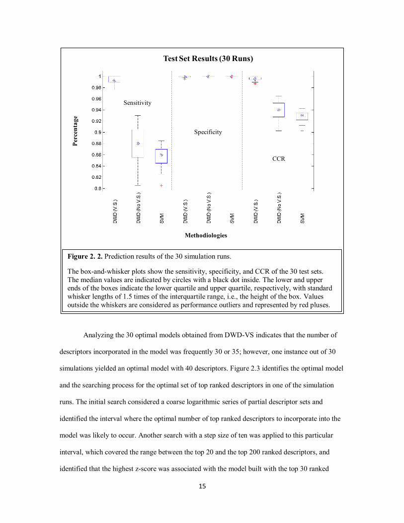
The prediction results of the test sets from the 30 simulation runs are summarized by the

box-and-whisker plots shown in Figure 2.2, which shows the sensitivity, specificity, and correct

classification rate (CCR) over the 30 test runs. The results of the simulation showed that all three

methods performed similarly in specificity. With the implemented variable selection (V.S.),

DWD consistently achieved a higher sensitivity and CCR than the other two methods.

15

Analyzing the 30 optimal models obtained from DWD-VS indicates that the number of

descriptors incorporated in the model was frequently 30 or 35; however, one instance out of 30

simulations yielded an optimal model with 40 descriptors. Figure 2.3 identifies the optimal model

and the searching process for the optimal set of top ranked descriptors in one of the simulation

runs. The initial search considered a coarse logarithmic series of partial descriptor sets and

identified the interval where the optimal number of top ranked descriptors to incorporate into the

model was likely to occur. Another search with a step size of ten was applied to this particular

interval, which covered the range between the top 20 and the top 200 ranked descriptors, and

identified that the highest z-score was associated with the model built with the top 30 ranked

Methodiologies

Per

cen

tag

e

Test Set Results (30 Runs)

Sensitivity

Specificity

CCR

Figure 2. 2. Prediction results of the 30 simulation runs.

The box-and-whisker plots show the sensitivity, specificity, and CCR of the 30 test sets.

The median values are indicated by circles with a black dot inside. The lower and upper ends of the boxes indicate the lower quartile and upper quartile, respectively, with standard

whisker lengths of 1.5 times of the interquartile range, i.e., the height of the box. Values

outside the whiskers are considered as performance outliers and represented by red pluses.

16

descriptors. One last search with a step size of 5 was performed in the region between the top 20

to the top 110 ranked descriptors in order to approximate the location of the optimal z-score.

To further analyze the performance of the implemented variable selection, recall and true

negative rate were calculated based on the descriptors selected by each of the optimal models

obtained from DWD-VS. The recall is the percentage of the 50 informative descriptors selected

Figure 2. 3. Identification of the optimal model through the z-score.

The initial search considered a coarse logarithmic series of partial descriptor sets and

identified the interval where the optimal number of top ranked descriptors to incorporate

into the model was likely to occur (left plot). Once the region of high z-scores was

identified, additional searches were performed with smaller increments of the number of

top ranked descriptors. In this particular run, the optimal model was the one that

incorporated the 30 top ranked descriptors (right plot).

17

by the model, and the true negative rate or the noise removal rate is the percentage of the noise

excluded by the model. The true negative rate for each of the 30 simulation runs was close to

100%; however, the recall for the informative descriptors ranged only from 0.58 to 0.78, with a

median of 0.60 (Figure 2.4). The recall and the true negative rate calculated from the 30

simulation run indicated that the implemented variable selection was capable of improving the

classification result by removing most of the noise while retaining the majority of the informative

descriptors.

The outcome of this simulation shows that the z-score proved to be a strong indicator

for model performance and a helpful parameter for model optimization. Since the calculation of

the z-score does not require setting aside additional data, the resulting models also have the

Model Analysis

Per

cen

tag

e

Recall True Negative Rate

Figure 2. 4. Model analysis of the simulated data.

In this simulation, the optimal model usually selected 30 out of the 50 informative

descriptors while removing most of the noise.

18

advantage of using all the data available. This advantage is critical for modeling the imbalanced

categorical dataset in the HDLSS setting.

2.6 QSAR Studies

For the QSAR studies, all three methods, i.e., SVM without VS and DWD both with and

without VS, were applied to build binary classification models for five different datasets. The first

dataset contains 110 compounds that include inhibitors and non-inhibitors for AmpC β-lactamase.

The other four datasets are the binders and non-binders for the different families of serotonin

receptors (5-HT receptors). For each of these datasets, Dragon 3 descriptors, which include both

physicochemical and structural properties of molecules, were generated. Descriptors with zero

variance were removed from the generated descriptor matrices. For highly correlated descriptors

within the descriptor matrix that achieve pairwise correlation close to 1.00 from one another, an

additional step was taken by selecting only one descriptor as representative. The resulting

descriptor matrix and the corresponding categorized biological activity for each dataset were

partitioned into modeling and test sets, and all three methods were built with the same modeling

sets and applied to the same test sets for the benchmark.

In QSAR studies, model validation is an important part of the workflow. To make the

model validation process more generalizable, a five-fold cross-validation procedure was applied

to the data partitioning of modeling sets and test sets (external validation set). Within each

modeling set, another five-fold cross-validation procedure was applied for model tuning by

further partitioning the modeling set into both training and validation sets (internal test set). To

distinguish the two procedures, the five-fold cross-validation procedures associated with model

validation and model tuning were denoted as five-fold external cross-validation and five-fold

internal cross-validation, respectively.

For all the QSAR studies in this research, five-fold internal cross-validation was applied

to estimate the optimal penalty parameters for both SVM and DWD. DWD was tuned without

19

variable selection and those tuning parameters were used throughout the variable selection

process. After the optimal penalty was identified through the five-fold internal cross-validation

process, a single model was then built based on the complete modeling set data (using the union

of the training set and the validation set). Each complete model was then applied to classify the

corresponding test set. To summarize the classification result of the test sets, the prediction

outcomes from the 5 test sets were combined. Sensitivity, specificity, and CCR were calculated

from this combined set of outcomes.

2.7 QSAR Datasets Description

2.7.1 AmpC β–lactamases Dataset Description (110 Compounds)

The β-lactam ring is an essential structure of several antibiotic families, such as the

penicillins, cephalosporins, carbapenems, and monobactams. Due to the commonality of this

particular active structural feature among these chemical compounds, they are collectively called

as the β-lactam antibiotics 66

. These chemical compounds gain their antibiotics status by

inhibiting bacterial cell wall synthesis. The inhibition of cell wall synthesis has a lethal effect on

bacteria, especially on the Gram-positive bacteria that are characterized by the high amount of

peptidoglycan in the cell wall. However bacteria can become resistant against β-lactam antibiotics

by expressing β-lactamase, an enzyme that is produced by Gram-negative organisms and has the

ability to break open the β-lactam ring thus deactivating the antibacterial properties. In 1940,

AmpC β-lactamse of Escherichia coli was the first bacterial enzyme reported to destroy penicillin

70. Since the discovery of the β-lactamases and their attributions toward antibiotic resistance, there

has been a significant amount of efforts in the scientific community to identify compounds that

inhibit β-lactamases to work in conjunction with antibiotics.

A dataset containing AmpC β-lactamases inhibitors and non-inhibitors was published by

Shoichet’s group 120

. In this data, competitive binding (Ki in µM) was measured for all the

molecules. Molecules with Ki less than 1,000 µM were considered inhibitors and molecules with

20

Ki greater or equal to 1,000 µM were considered non-inhibitors. The range of inhibition (Ki

values) is from 1.0 to 646.0 µM. Molecules with smaller Ki are considered strong inhibitors but

for the classification, there is no distinction between strong inhibitors and weak inhibitors. The

published data contains 21 inhibitors and 84 non-inhibitors. Additional data were later provided

by Shoichet’s group that includes five additional inhibitors of the same chemical series.

2.7.2 5-HT Datasets Description

The serotonin receptors, also known as 5-Hydroxytryptamine (5-HT) receptors,

influence various biological and neurological processes such as aggression, anxiety, appetite,

cognition, learning, memory, mood, nausea, sleep, and

thermoregulation. The serotonin receptors are the target of

a variety of pharmaceutical and illicit drugs, including

many antidepressants, antipsychotics, anorectics,

antiemetics, gastroprokinetic agents, antimigraine agents,

hallucinogens, and entactogens [3].

There are 7 different 5-HT receptor families: 5-

HT1, 5-HT2, 5-HT3, 5-HT4, 5-HT5, 5-HT6, and 5-HT7.

These 5-HT receptor families can be further characterized

in subtypes (shown in Table 2.1). With the exception of the

5-HT3 receptors, which are ligand-gated ion channel, all

other serotonin receptors are G protein-coupled receptors

that activate an intracellular second messenger cascade to

produce an excitatory or inhibitory response.

A collection of binders and non-binders associated with 5-HT1B, 5-HT1D, 5-HT2B, and 5-

HT6 receptors are obtained from PDSP 112

. In the collected data, there are 91 binders and 79 non-

binders associated with 5-HT1B receptors. As for 5-HT1D receptors, the numbers are 87 and 81 for

Family Subtype

5-HT1A

5-HT1B

5-HT1D

5-HT1E

5-HT1F

5-HT2A

5-HT2B

5-HT2C

5-HT3 5-HT3

5-HT4 5-HT4

5-HT5 5-HT5A

5-HT6 5-HT6

5-HT7 5-HT7

5-HT1

5-HT2

Table 2. 1. 5-HT receptor

families and subtypes.

21

binders and non-binders respectively. Comparison between the binders of 5-HT1B and 5-HT1D

receptors indicates 70 overlapping binders that bind to both receptors. However, there is no

evidence in the data to suggest that the non-overlapping binders are specific to their

corresponding receptors.

2.8 QSAR Modeling Results

2.8.1 AmpC Β-lactamase Modeling Result (110 Compounds)

In total 894 two-dimensional (2D) molecular descriptors were generated for these 110

compounds with commercially available software, Dragon 3. As mentioned earlier (Section 2.6),

five-fold external cross validation was implemented to perform the QSAR study for this dataset.

The classification results of the five test sets were combined into a single set to calculate the

DWD with Variable Selection

DWD withoutVariable Selection

SVM

Sensitivity Specificity CCR

Per

cen

tag

e

Combined Result of Test Sets

(AmpC Dataset)

Figure 2. 5. Performance comparison between the methods (AmpC dataset).

The bar graph shows the test set result of the five-fold external cross validation. The

predictions for each of the five test sets were combined into a single set to calculate the

sensitivity, specificity, and CCR. In the AmpC dataset, both DWD methods achieve

better classification outcomes than SVM; however, the classification results between the

two DWD methods are quite similar.

22

sensitivity, specificity, and CCR (shown in Figure 2.5). The three methods performed similarly in

classifying the inhibitors vs. non-inhibitors in the test sets. Compared to SVM, DWD with

variable selection was able to give correct predictions for one additional inhibitor and two non-

inhibitors. The difference in specificity between the two DWD methods was caused by the correct

prediction of one non-inhibitor. The small difference in classification performance could be

explained by the structure similarities of the

inhibitors. The chemical structures of the majority

of inhibitors in this dataset belonged to a

chemotype that can be characterized by a

sulfonamide bridging two aromatic rings, with

one aromatic ring containing a carboxylic

functional group. Molecular descriptors reflecting

the characteristic of this chemotype were highly

ranked in both DWD and DWD-VS, thus causing

the similarity in classification performance

between the two methods. However, DWD-VS

did have an advantage over the DWD in model

interpretation by identifying a much smaller set of

descriptors that are significant to a biological

property.

Analyzing the models obtained from

DWD-VS indicated that the numbers of

descriptors incorporated in each of the five folds

were 100, 150, 150, 250, and 100. Cross-checking

these descriptors yielded 315 unique descriptor

Mp nSO2N

nS nThiophenes

T(O..S) C-027

MATS4v C-029

MATS3e C-033

MATS4e C-034

MATS6e H-047

MATS4p H-048

GATS2m H-049

GATS1v O-057

GATS2v O-060

GATS4v N-067

GATS5v N-075

GATS6v Inflammat-80

GATS5e Infective-50

GATS6e F01[C-N]

GATS4p F01[N-S]

EEig01x F02[C-S]

BELm3 F03[C-O]

BEHe8 F03[N-S]

BEHp1 F04[N-O]

BELp3 F04[N-S]

JGI9 F04[O-S]

nArCOOH F05[O-O]

nArCONHR

Descriptor Name

Table 2. 2. The 49 unique descriptors selected by all 5 models.

The highlighted descriptors reflect the

common structure features that

distinguished the inhibitors from the

non-inhibitors.

23

names. Among these unique descriptors, 49 were selected by all the five models. These 49

descriptors are shown in Table 2.2.

Although not all the descriptors from Dragon are easily interpretable, some can be easily

mapped back to the molecules. For example, nSO2N, nThiophenes, and nArCOOH are the

descriptors that reflect the common structure features of the inhibitors. Visual inspection of the

inhibitors indicates that the molecular structures usually contain a sulfonamide linking two

aromatic substituents (Figure 2.6). One of the aromatic substituents should include a carboxylic

acid. These observations match with the descriptors selected by the models. The nArCOOH is a

descriptor that indicates the occurrence of an aromatic substituent with carboxylic acid in a

molecule. As for nSO2N and nThiophenes, these are the occurrences of sulfomamide and

thiophene respectively.

Figure 2. 6. Common structure features of the AmpC inhibitors.

Most of the inhibitors have a sulfonamide (orange) linking two aromatic substituents. One

aromatic substituent must contain a carboxylic acid (blue). Thiophene (purple) is

considered as an aromatic substituent.

24

2.8.2 5-HT1B Modeling Result

In total 875 2D Dragon descriptors were generated for the 170 structurally diverse

compounds. Building global models yielded poor and inconsistent classification performance

across the folds. To improve the classification performance, the modeling approach was to

partition the data into clusters and to build specific models for each cluster.

Unsupervised

clustering analysis of the

170 compounds was

performed based on the

875 chemical descriptors.

A dendrogram was

constructed based on

hierarchical clustering

with Ward linkage

(Figure 2.7). The

dendrogram indicates

how the data can be

subdivided into clusters.

Local models were built

by clustering the data into either 2 or 3 groups. Building local models for the three clusters

yielded better and more consistent results than building local models for the two higher level

clusters. In order to obtain some insight regarding the clusters, a principal component analysis

(PCA) plot was generated to visualize the distributions of both clusters and different classes of

compounds (Figure 2.8).

Figure 2. 7. Dendrogram of the 5-HT1B dataset.

Hierarchical clustering (with Ward linkage) was performed for

the dataset based on the chemical descriptors. The dendrogram

indicates how the data can be subdivided into clusters. For

building local models, the data were subdivided into either two or three clusters.

25

There are 41 binders and 35 non-binders in the red cluster. The green cluster contains 18

binders and 24 non-binders. As for the blue cluster, the numbers of binders and non-binders are

32 and 20 respectively. Five-fold external cross-validation procedure was applied for each cluster.

However, the cluster labels were only applied for the training sets and not the test set.

To predict the compounds in the test sets, a neighborhood search was performed in the

full descriptor space. For each compound in the test set, its nearest neighbor in the training set

was identified. The decision of model selection for predicting a given test set compound was

based on the nearest training set compound in each cluster. For any given data in the test set, its

nearest neighbor in the training set will determine the cluster membership. Based on the cluster

Figure 2. 8. Data distribution of the 5-HT1B dataset in Dragon chemical descriptor space.

The different colors (red, blue and green) in the plots indicate the three clusters identified in

hierarchical clustering. Binders and non-binders are represented as circles and crosses

respectively. In the two clusters scheme, the data in green and red are merged into a single cluster.

26

membership, the corresponding local model will be applied for prediction. The classification

results from the five-fold external cross-validation of the three clusters were combined into a

single set to calculate the sensitivity, specificity, and CCR. As indicated by the results in Figure

2.9, all three methods performed well after clustering the 5-HT1B data. DWD-VS was able to

correctly predict five more binders than SVM and DWD without variable selection. SVM also

misclassified five more non-binders than either DWD method.

Analyzing the descriptors incorporated in the optimal models from DWD-VS yielded 169

unique descriptors for the red cluster, 173 for the green cluster, and 119 for the blue cluster.

Among the 169 unique descriptors identified for the red cluster, there are 26 descriptors which



SVM


Per

cen

tag

e


(5-HT1B Dataset)

Figure 2. 9. Performance comparison through five-fold external cross validation for the 5-

HT1B dataset.

For both the 5-HT1B and the 5-HT1D datasets, local models were built based on the clusters

suggested by hierarchical clustering. Selection of a model to predict a compound in the test

set was based on identifying its most similar compound in the training compounds. All

three methods performed well in this 5-HT1B dataset.

27

showed up in all models. For the green and blue clusters, the numbers of unique descriptors

selected by all models were 33 and 12, respectively. These selected descriptors are listed in Table

2.3 according to the membership of the clusters. The overlap of selected descriptors between

clusters was minimal. Between the green and the blue clusters, the two descriptor lists did not

overlap. Five descriptors, which are nR12, nRNR2, C-006, N-068, and O-56, were incorporated

in all the models for both red and blue clusters. As for the red and green clusters, both

incorporated the descriptors, nRCOOH and nPyrroles, in all of their respective models.

nR10 N-068

nR12 N-069

D/Dr10 N-073

JGI9 Inflammat-50

JGI10 Neoplastic-50

nRCOOH Infective-50

nRNR2 F03[N-O]

nArOH F04[C-S]

nOHs F05[C-S]

nROR F05[N-N]

nPyrroles F07[O-S]

C-006 F08[N-S]

O-056 F09[N-O]

Descriptor Name (Red Cluster)

ARR nCrt

nDB nRCOOH

nO nROH

nF nPyrroles

nX C-003

PJI2 C-013

piPC10 C-033

PCR C-040

EEig01x O-058

ESpm14x F-083

ESpm15x F02[C-F]

ESpm01d F02[O-O]

BEHv1 F03[C-F]

BEHe1 F04[C-F]

BEHp1 F05[C-F]

JGI8 F07[N-F]

nCt

Descriptor Name (Green Cluster)

nR12 C-008

T(N..N) C-040

nCs H-046

nCrs O-056

nRNR2 N-068

C-006 F10[C-N]

Descriptor Name (Blue Cluster)

Table 2. 3. The unique descriptors

selected by all 5 models from each of the three clusters.

28

2.8.3 5-HT1D Modeling Result

In total 870 2D Dragon descriptors were generated for the 168 structurally diverse

compounds. Similar to the outcome for the 5-HT1B dataset, local models yielded better

classification performance than global models. Hierarchical clustering of the 5-HT1D dataset with

Ward linkage produced

the following

dendrogram (Figure

2.10). Due to a

significant amount of

overlapping compounds

between the 5-HT1B and

the 5-HT1D datasets,

local models were built

based on clustering the 5-

HT1D dataset into 3

groups in an attempt to

compare the results. The

PCA plot below shows the data distribution of the 3 clusters in the chemical space (Figure 2.11).

The data distribution of 5-HT1D in the PCA plot is similar to that of the 5-HT1B. The largest

cluster (red cluster) contains 61 binders and 41 non-binders while the smallest cluster (green

cluster) includes 11 binders and 16 non-binders. As for the blue cluster, the numbers of binders

and nonbinders are 15 and 24, respectively.

Figure 2. 10. Dendrogram of the 5-HT1D dataset.

Due to a significant amount of overlapping compounds between

the 5-HT1B and the 5-HT1D datasets, local models were built by

clustering the 5-HT1D dataset into 3 groups in an attempt to compare the results.

29

Five-fold external cross-validation procedure was applied to each of the cluster to obtain

the corresponding optimized models. Once again, the cluster labels were only applied for the

training sets and not the external test set. To predict the compounds in the test sets, a

neighborhood search was performed in the full descriptor space. For any given data in the test set,

its nearest neighbor in the training set will determine the cluster membership. Based on cluster

membership, the corresponding local model will be applied for prediction. The classification

results from the five-fold external cross-validation of the three clusters were combined into a

single set to calculate the sensitivity, specificity, and CCR. As indicated by the results in Figure

Figure 2. 11. Data distribution of the 5-HT1D dataset in Dragon chemical descriptor space.

The different colors (red, green, and blue) in the plots are to indicate the three clusters

identified in hierarchical clustering. Binders and non-binders are represented as circles and crosses respectively. In the two clusters scheme, the data in green and red are in a single

cluster. The relative position of the three clusters identified for the 5-HT1D dataset is similar

to the three clusters associated with 5-HT1B.

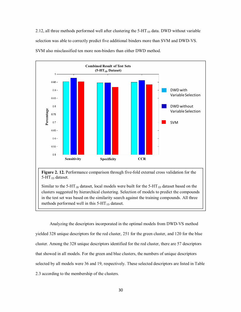
30

2.12, all three methods performed well after clustering the 5-HT1D data. DWD without variable

selection was able to correctly predict five additional binders more than SVM and DWD-VS.

SVM also misclassified ten more non-binders than either DWD method.

Analyzing the descriptors incorporated in the optimal models from DWD-VS method

yielded 328 unique descriptors for the red cluster, 251 for the green cluster, and 120 for the blue

cluster. Among the 328 unique descriptors identified for the red cluster, there are 57 descriptors

that showed in all models. For the green and blue clusters, the numbers of unique descriptors

selected by all models were 36 and 19, respectively. These selected descriptors are listed in Table

2.3 according to the membership of the clusters.



SVM


Per

cen

tag

e


(5-HT1D Dataset)


5-HT1D dataset.

Similar to the 5-HT1B dataset, local models were built for the 5-HT1D dataset based on the

clusters suggested by hierarchical clustering. Selection of models to predict the compounds

in the test set was based on the similarity search against the training compounds. All three

methods performed well in this 5-HT1D dataset.

31

nO nPyrrolidines

nX nPyrroles

nR09 C-006

TI2 C-007

D/Dr07 C-027

D/Dr09 C-033

D/Dr10 C-034

T(O..S) C-040

MATS1p H-049

GATS5m H-052

GATS4v N-068

GATS5v N-069

GATS4e N-075

GATS5e Depressant-80

GATS1p Hypertens-50

EEig01x Hypnotic-50

ESpm12x Neoplastic-80

ESpm13x Neoplastic-50

ESpm14x F01[C-N]

ESpm15x F01[C-O]

BEHv1 F03[C-S]

BEHe1 F03[N-O]

BEHp1 F04[C-S]

VEA1 F05[S-Cl]

nCrs F06[N-Cl]

nRCOOH F07[N-N]

nCONN F07[N-O]

nRNR2 F08[N-S]

nArX

Descriptor Name (Red Cluster)

ARR GATS7p

nN EEig13d

nF EEig14d

nX nCRX3

PW5 nPyrroles

piPC10 C-013

X3A C-033

MATS6m O-058

MATS5v N-073

MATS5e F-083

MATS6p GVWAI-80

GATS6m F01[C-F]

GATS7m F02[F-F]

GATS6v F03[C-F]

GATS7v F04[C-F]

GATS6e F05[C-F]

GATS7e F05[N-N]

GATS6p F07[N-F]

Descriptor Name (Green Cluster)

nN C-008

nR09 C-012

TI2 C-013

D/Dr09 N-067

T(N..N) F01[C-N]

nCs F07[N-N]

nCrs F08[C-N]

nRNHR F09[C-N]

nRNR2 F10[N-O]

C-006

Descriptor Name (Blue Cluster)

Table 2. 4. The unique descriptors selected by all 5 models from each of the three

clusters.

The highlighted descriptors are selected by the similarly located clusters in both 5-HT1B

and 5-HT1D.

32

Comparing these descriptors with those of the similarly located clusters in 5-HT1B

indicated some overlapping descriptors. There were nine descriptors that appeared in both red

clusters. The numbers of overlapping descriptors between the two datasets were 12 and 6 for the

green and blue clusters, respectively. Understanding the contribution of these overlapping

descriptors to the binding of 5-HT1B and 5-HT1D receptors could contribute to designing a safer

drug.

2.8.4 5-HT2B Modeling Result

In total 1,030 Dragon 2D descriptors were generated for these 753 compounds. The

classification results of the five-fold external cross validation were combined into a single set to

calculate the sensitivity, specificity, and CCR (shown in Figure 2.13). The difference in

classification results between the three methods is minimal. Both DWD methods had higher



SVM


Per

cen

tag

e


(5-HT2B Dataset)

Figure 2. 13. Performance comparison through five-fold external cross validation for the 5-HT2B dataset.

For the 5-HT2B dataset, both DWD methods yielded similar performance in classifying

binders vs. non-binders from the test sets. In comparison, the sensitivity associated with

SVM did show a drop in performance.

33

sensitivity and specificity than SVM. Comparison with SVM, DWD-VS was able to provide

correct predictions for four additional binders and six non-binders. The differences in sensitivity

and specificity between the two DWD methods were caused by the correct predictions of two

binders and four non-binders.

Analyzing the models

obtained from DWD-VS

indicated that the numbers of

descriptors incorporated in

each of the five folds were

250, 250, 200, 400, and 200.

Cross-checking these

descriptors yielded 482

unique descriptor names.

Among these unique

descriptors, 79 were selected

by all the 5 models. These 79

descriptors are shown in

Table 2.5.

Ms BELm6 H-049

nO BEHv1 N-070

nR07 BELv6 N-071

nR10 BELe6 N-074

nR11 BEHp1 Cl-086

Lop JGI2 Ui

D/Dr11 JGI3 Psychotic-50

T(N..F) JGI7 F02[C-O]

PCR JGI8 F03[N-F]

X0Av nCrq F04[N-Cl]

IC2 nCb- F05[N-N]

SIC2 nR=Cs F05[N-O]

CIC2 nR#CH/X F05[N-Cl]

BIC2 nRCOOR F05[S-Cl]

MATS1m nArCOOR F07[C-F]

MATS4m nArOCON F08[C-N]

MATS5m nC(=N)N2 F08[N-S]

GATS2m nArNHR F09[C-N]

GATS3m nArNR2 F09[O-O]

GATS7v nRCN

GATS8v nOHs

GATS3e nArOR

GATS2p nSO2N

GATS3p nPyrroles

EEig05x nPyridines

EEig06x C-006

EEig07x C-013

EEig09d C-021

EEig11d C-028

EEig09r C-033

Descriptor Name

Table 2. 5. The 79 unique descriptors selected by all 5 models for the 5-HT2B dataset.

34

2.8.5 5-HT6 Modeling Result

In total 1,233 2D Dragon descriptors were generated for these 176 compounds. The

classification results of the five-fold external cross validation were combined into a single set to

calculate the sensitivity, specificity, and CCR (shown in Figure 2.14). The classification results of

the three methods revealed similar performance in classifying the binders vs. non-binders. DWD-

VS was able to predict one additional binder and 4 non-binders more than the other two methods.



SVM


Per

cen

tag

e


(5-HT6 Dataset)


5-HT6 dataset.

For the 5-HT6 dataset, DWD with variable selection showed better classification

performance than the other two methods.

35

Analyzing the models obtained from DWD-VS indicated that the numbers of descriptors

incorporated in each of the five folds were 400, 300, 250, 200, and 250. Cross-checking these

descriptors yielded 505 unique descriptor names. Among these unique descriptors, 87 were

selected by all the 5 models. These 87 descriptors are shown in Table 2.2.

ARR nNq Inflammat-50 B09[O-O]

nDB nArOH Depressant-50 B10[C-C]

nAB nPyrroles Neoplastic-80 B10[C-O]

nBnz C-001 Neoplastic-50 F01[C-N]

D/Dr09 C-004 Infective-80 F02[C-S]

MATS5m C-005 BLTF96 F03[N-S]

MATS1v C-006 BLTD48 F04[C-S]

GATS7v C-008 BLTA96 F06[C-N]

GATS5e C-013 B02[N-O] F06[N-Cl]

GATS7e C-025 B03[N-N] F07[C-N]

GATS8p C-027 B03[N-O] F07[N-S]

EEig03d C-031 B03[N-S] F08[C-Cl]

JGI9 C-034 B04[N-S]

JGI10 C-040 B04[O-O]

nCp H-046 B05[N-O]

nCs H-047 B06[C-N]

nCq H-049 B06[N-Cl]

nCrs O-057 B07[C-S]

nCar O-058 B07[N-S]

nCb- N-073 B07[O-O]

nRCONHR N-079 B08[C-N]

nRCONR2 Ui B08[C-O]

nN=C-N< MLOGP B08[N-N]

nArNR2 ALOGP2 B08[O-O]

nN+ GVWAI-80 B09[C-F]

Descriptor Name

Table 2. 6. The 87 unique descriptors selected by all 5 models for the 5-HT6

dataset.

36

2.9 Conclusion

The results obtained on simulated data clearly indicated that DWD with variable selection

(DWD-VS) could significantly improve the model prediction performance for datasets that are

imbalanced and HDLSS. DWD-VS consistently achieved the highest prediction performance, and

both DWD methods showed better classification performance than SVM in predicting the test set

data. Analysis of DWD-VS models indicated that the high prediction accuracy was consistently

achieved by nearly 100% noise removal while retaining the majority of the informative

descriptors. In the modeling of real QSAR datasets, DWD-VS was consistently better than SVM

and had superior or similar performance to DWD without variable selection.

Analysis of descriptors incorporated in DWD-VS models suggested that the selected

descriptors could explain the contribution of a molecular structure feature to the desired target

biological property. This is especially evident in the modeling result of the AmpC β-lactamase

dataset, where the three descriptors, nArCOOH, nSO2N, and nThiophenes, reflect common

structure features of the inhibitors. Thus, DWD-VS can be used to obtain a better understanding

of the underlying process that generated the data. Compared to DWD without variable selection,

DWD-VS provided more cost-effective models by identifying predictor variables while achieving

high prediction accuracy, i.e. identifying a smaller number of descriptors that are significant to a

biological property.

Chapter 3

Novel Three-Dimensional Chirality Atom-Pair Descriptors

3.1 Motivation / Background

Many biologically-active compounds

are in fact chiral, and their stereochemistries

are believed to directly influence their

bioactivities because these compounds

(ligands) are recognized differently by their

corresponding receptors which are also chiral.

A molecule is said to be chiral when it cannot

be superimposed on its mirror image.

Chirality can be defined either by the

molecular optical activity or by the

configuration of the molecule. When optical

activity is considered, (+) or (-) notations are

used to distinguish the chiral compounds

from their mirror images. D/L or R/S

notations can alternatively be used to distinguish the enantiomers if chirality of the molecule is

defined by its molecular configuration instead (illustrated in Figure 3.1). The assignment of the

D/L system is based on the association between chiral molecules and glyceraldehydes. As for the

R/S system, it is determined by the Cahn-Ingold-Prelog priority rules. It is interesting to point out

Figure 3. 1. Two enantiomers of a generic

amino acid.

Pairs of enantiomers are often designated as

“right-“ or “left-handed.” Multiple notations can be used to differentiate one enantiomer

from the other.

Source:

http://en.wikipedia.org/wiki/File:Chirality_with_hands.jpg

38

that there is no fixed relation to the three labeling system. For example, an R isomer can be either

dextrorotatory or levorotatory, depending on its exact substituents.

Before the 1980s, the pharmacopoeia was dominated by compounds in the form of

racemic mixtures, but a breakthrough in technology enabling pure enantiomers to be generated in

significant quantities has not only revolutionized the pharmaceutical industry but also has raised

the awareness of and interest in the stereochemistry of drug action 6;29;30;53

. It is frequently the

case that one enantiomer is responsible for the activity of interest while its paired enantiomer is

found to be inactive but does share some other desirable or undesirable activities of interest.

Benefits such as reduction of the total administered dose, enhancement of the therapeutic window,

and a more precise estimation of dose–response relationships have been identified as the

advantages of using stereochemically pure drugs 6;29;30

. As a result, single enantiomers are

preferred by both industry and regulatory authorities, such as the US Food and Drug

Administration (FDA). In 1992, the FDA published a formal guideline regarding the development

of chiral drugs in a document entitled Development of New Stereoisomeric Drugs. As stated in the

document, “The stereoisomeric composition of a drug with a chiral center should be known and

Figure 3. 2. Growing trend of chiral technology.

According to a study by Frost & Sullivan, worldwide revenues related to chiral technology,

which amounted to $4.8 billion in 1999, were expected to be $14.9 billion in 2009 2.

39

the quantitative isomeric composition of the material used in pharmacologic, toxicologic, and

clinical studies known. Specifications for the final product should assure identity, strength,

quality, and purity from a stereochemical viewpoint.” 55

The growing trend for worldwide sales of chiral drugs in single-enantiomer forms is

expected to continue. In 1996, the worldwide annual sales of chiral drugs amounted to $74.4

billion, which constituted more than one-fourth of all drug sales; the number exceeded $159

billion in 2002 30;113;114;125-128

and the sales figure was projected to reach $200 billion in 2008 128

.

Brand

Name

Generic

Name

Therapeutic

Area

Pharmaceutical

Company

Lipitor Atorvastatin calcium Cardiovascular Pfizer

Zocor Simvastatin Cardiovascular Merck

Pravachol Pravastatin sodium Cardiovascular Bristol-Myers Squibb

Paxil Paroxetine hydrochloride Central Nervous

System GlaxoSmithKline

Plavix Clopidogrel bisulfate Hematology Sanofi-Synthelabo /

Bristol-Myers Squibb

Zoloft Sertraline hydrochloride Central Nervous

System Pfizer

Advair HFA Fluticasone propionate and

salmeterol xinafoate Respiratory GlaxoSmithKline

Nexium Esomeprazole magnesium Gastrointestinal AstraZeneca

Augmentin Amoxicillin and potassium

clavulanate Antibiotic GlaxoSmithKline

Diovan Valsartan Cardiovascular Novartis

Table 3. 1. List of top ten single enantiomer blocker drugs in ranking order.

Drugs must exceed the amount of $ 1 billion dollars in annual sales to be qualified as

blockbuster drugs. The global combined sales of Lipitor and Zocor almost reached 14

billion in 2002 2;30;114.

40

According to a study by Frost & Sullivan in 2001, worldwide revenues related to chiral

technology (equipment), which amounted to $4.8 billion in 1999, is expected to reach $14.9

billion in 2009 (Figure 3.2). Table 3.1 lists the top ten single enantiomer blockbuster drugs that

achieve more than $ 1 billion in sales per year.

3.2 Overview of Current Chirality Descriptors

As summarized by Crippen 42

, current chirality descriptors applied in the field of QSAR

can be classified as either qualitative or quantitative descriptors. To characterize chirality

quantitatively, three different computational implementations have been applied. The first

implementation is to calculate the overlap of the Van Der Waals volume or electrostatic potential

by superimposing a pair of enantiomers 28;93;117

. Another quantitative implementation is achieved

by measuring the degree of distortion, which can be characterized by calculating the distance

required to convert the molecule or subsets of its atoms into a structure with a desired symmetry,

such as mirror symmetry 7;11;45;148;149

. The third implementation to quantitatively characterize

chirality is achieved by translating and rotating the molecule to a standard position associated

with symmetry axes that are based on various atomic properties 49;91;94;145

.

Qualitative chirality descriptors, on the other hand, are typically based on the

mathematical concept of oriented volume and with the notational viewpoint of the Cahn-Ingold-

Prelog rules 60;61;72;146

. Instead of focus on atomic number, qualitative chirality descriptors could

place emphasis on other properties, such as electronegativity, polarizability, resonance

stabilization, etc 34;75;80;104;150

.

The idea of characterizing chirality has sparked a lot of imaginative work by many

scientists over the years. Both quantitative and qualitative chirality descriptors have been shown

to build successful models in QSAR studies. However, as suggested by Crippen, it has not yet

been determined how to best apply these descriptors in QSAR applications 42

.

41

3.2.1 Prior Implementation of the Chirality Descriptors

Several series of chirality descriptors of chemical organic molecules have been developed

earlier in this laboratory 60;61;76

. These descriptors have been used to build predictive quantitative

structure-activity relationship (QSAR) models for several datasets 60-62;74-76

and were developed

on the basis of conventional topological descriptors of molecular graphs. Chirality descriptors

emphasized on electronegativity instead of atomic number were particularly intriguing due to the

fact that receptor-ligand interaction is affected by factors such as Van Der Waals interactions,

hydrophobic interactions, and electrostatic interactions.

The concept of chirality based on partial charges, which capture the electrostatic

interactions at the atomic level, was introduced by Kovatcheva, et al. to study a set of chiral

ambergris fragrance compounds 75

. Similar to

the traditional R/S notation, which follows the

Cahn-Ingold-Prelog priority rules, the

configuration of the molecule was rearranged

in such a way that the neighboring atom with

the lowest partial-charge was projected

toward the back of the plane formed by the

remaining 3 neighboring atoms. The three

neighboring atoms within the plane can either

be in a clockwise or counter-clockwise

rotation if moving from the atom with the

highest partial charge among the three to the

lowest one. The chiral atom would be labeled

as R* for clockwise rotation and S

* for

counter-clockwise. In a previous study, the

Atom Types Description

01 Negative Point Center

02 Positive Point Center

03 Hydrogen Bond Acceptor

04 Hydrogen Bond Donor

05 Aromatic Ring Center

06 Nitrogen (All)

07 Oxygen (All)

08 Sulfur (All)

09 Phosphor (All)

10 Fluorine

11 Chlorine, Bromine, Iodine

12 Carbon

13 Other Elements

14 Triple Bond Center

15 Double Bond Center

16 Chiral Atom R*

17 Chiral Atom S*

Table 3. 2. The 17 atom types defined in the atom pair descriptors.

Regular atom pair descriptors contain atom

types 01 to 15 while chirality atom pair

descriptors contained all the atom types in

regular atom pair descriptors (with two

additional atom types - 16 and 17).

42

method of choice to calculate partial change in order to define atomic chirality was Gasteiger-

Hükkel 75

. Additionally, minimum graph distance, which is derived from a 2D molecular

structure, was used to define molecular features.

Chiral atom types defined above were incorporated as new atom types for calculation of

atom-pair descriptors, based on an approach proposed by Carhart et al. 32

. Atom-pair descriptors

encoded the molecular graph patterns defined by atom types and topological distance bins. These

contained the number of occurrences for each particular pattern. A molecular pattern in atom-pair

descriptors was a substructure path separation (or graph distance) between the atoms:

<Atom type I><Atom type II>_<distance between atom types>

The distance between any two atom types was defined as the minimum graph distance. The

minimum graph distance is the smallest amount of bond distance along the path between any two

specified atom types within a molecular structure (2D distance). The value encoded within the

atom-pair descriptors contained the number of occurrences associated with a particular pattern as

defined by a pair of atom types within a certain distance (binned distance) away. Listing of all 17

atom types implemented in the atom-pair descriptors was shown in Table 3.2.

3.2.2 Three Dimensional Chiral Atom-Pair Descriptors

A shortcoming associated with the prior implementation of the atom-pair descriptors was

related to the minimum graph distance (2D distance). The molecular patterns defined by the

minimum graph distance could not capture the difference between the trans- and cis-

configurations of molecules that could have dissimilar biological property. By not capturing the

subtle structural differences in the molecular configurations, the descriptors became limited in the

QSAR studies.

To address this shortcoming, the distance bin that defined the molecular patterns was

changed from 2D distance to three-dimensional (3D) distance, which was calculated by taking the

Euclidean distance of the atom coordinates in the physical space (3D space). However, a

43

limitation associated with 3D molecular descriptors (a set of features describing molecules in 3D)

is the fact that the method is conformation dependent. Depending on the structural rigidity of a

given molecule, multiple different 3D representations (conformations) can be generated. In order

to get a single structural representation for each compound, one common approach is to use the

minimum energy conformer, which may not accurately capture the binding conformation of the

ligand, especially when the given compounds are very flexible. In fact, there is no a priori reason

to exclude higher energy conformers as a source of activity.

Another alternative to the 3D descriptors generated from a single conformation would be

deriving the 3D descriptors from multiple conformers of a molecule, which requires a

conformation search of all the molecules. A conformation search was achieved through the

OMEGA 100

software by OpenEye. The search criteria implemented in this study included the

generation of a maximum of 50,000 possible conformations for each molecule. For molecules

containing less than or equal to 4 rotors, the associated conformers were considered duplicated if

the minimum Root Mean Square (RMS) Cartesian distance was less than 0.8. The RMS cutoff

value was increased to 1.15 for molecules containing more than 4 rotors. A maximum of 1,000

conformations satisfying the selection criteria were retained. However, the number of resulting

conformers could be less than 1,000 if a compound was structurally rigid.

After the completion of a conformation search, 3D chiral atom-pair descriptors were

generated for each conformer. Since multiple conformers were associated with a single molecule,

each molecule would be characterized by a molecular pattern matrix, where the rows represented

the conformers and the molecular patterns associated with each conformer were represented by

the columns. To summarize the molecular pattern matrix associated with each molecular entry,

taking the Boltzmann average of the molecular pattern matrix could derive a single 3D

descriptors vector for a given molecule 80

. However, using the Boltzmann average placed higher

emphasis on the conformers with much lower energy.

44

Rather than using the Boltzmann average to derive the final 3D descriptor vector for a

given molecule, three different values, which were the maximum, the arithmetic mean, and the

percentage of zero values (the percentage of conformers that lack the particular feature), were

used to characterize the distribution of each descriptor value with the given number of conformers.

The choice of an arithmetic mean over the Boltzman average meant that the possibilities for all

the resulting conformers to be in the bioactive form were all equally likely.

In addition to the change of the distance type that defined the molecular patterns, the 3D

chiral atom-pair descriptor matrix incorporated the concept of the degree of chirality, which is a

threshold used to define the chiral atom types. In order for a carbon atom to be considered as a

chiral atom, the minimum difference in the atomic partial charge between any two of the four

connecting atoms must be greater than this threshold. By varying this threshold, multiple 3D

atom-pair descriptor matrices with different degree of chirality could be generated but only

molecular patterns involving atom type 12, 16, and 17 were affected by the threshold. By

incorporating the degree of chirality concept, it is possible to identify a subset of chiral carbon

atoms and their association with the target properties.

In the earlier study, a carbon atom would be considered as a chiral atom type if all four of

its connecting atoms were different and the method of choice to calculate partial charge was

Gasteiger-Hükkel 75

. The partial charge calculation in this study was accomplished by the

QUACPAC 99

software from OpenEye, which suggested AM1-BCC to be the model of choice for

calculating partial charge due to the better performance on predicting protein-ligand binding

calculations and virtual screening through docking methods. The calculation scheme for AM1-

BCC was to calculate the initial partial charges derived from the AM1 semi-empirical method,

followed by bond-charge corrections (BCC) to generate the final atomic partial charges.

To avoid incorporating the non-chiral atoms as defined by the International Union of

Pure and Applied Chemistry into the chiral atom types in the 3D chiral atom-pair descriptors, the

minimum threshold to define chiral atoms was set to 0.0010. Additional thresholds were

45

evaluated by setting the maximum value to 0.0290 with a step size of 0.0020. Thus a total of 15

different thresholds were evaluated. With higher threshold value, the number of chiral atoms in

the new definition will be smaller.

3.3 Dataset Description

3.3.1 Peptide Transporter 1 (PEPT1) Dataset

Peptide transporter 1 (PEPT1), localized to the brush border membrane of the intestinal

epithelium, is a solute carrier for oligopeptides and transports nutritional di- and tripeptides across

the luminal membrane into small intestinal cells 4;5;133

. In addition to the oligopeptides, other

peptidomimetics, which are molecules designed to mimic peptides, are also transported by PEPT1.

The ability of PEPT1to transport peptidomimetic drugs, such as β-lactam antibiotics, valacyclovir,

δ-amino-levulinic acid, angiotensin-converting enzyme inhibitors, and bestatin, allows the oral

application of these drugs for the therapy of several diseases 13;24-26;48;56;57;64;96;129;130;132;134;151

.

Targeting the membrane transport protein PEPT1 to enhance the oral bioavailability of

drugs is a promising strategy; however, very little is known about the substrate binding pocket of

PEPT1. To gain some insights regarding the structural requirements for the PEPT1 binding

substrates, cheminformatic analysis, such as QSAR, can be applied to identify key molecular

structure features that are contributing to the binding of PEPT1.

A dataset published by Biegel et al 20

, which contained 122 compounds (substrates) and

their corresponding binding affinity values (Ki values) to PEPT1, was retrieved from the

ChEMBL database. Among the 122 PEPT1 binding substrates, there were 31 β–lactam antibiotics,

32 tripeptides, and 59 dipeptides. For tripeptides and dipeptides, different amino acid sequences

were measured experimentally for their binding affinity. The experimentally measured Ki values

also included polypeptides (tripeptides and dipeptides) with amino acids that were strategically

substituted with D-enantiomers. Tripeptides in LLL configuration display a higher affinity to

PEPT1 (with Ki values ranging from 0.1 to 0.5 mM) compared to tripeptides in DLL, LDL, and

46

LLD configurations. This stereochemical preference is also observed in dipeptides, which

preferred LL more than DL, LD, or DD. However the binding affinity value for the tripeptide, D-

Met-Met-Met, also indicated high affinity to PEPT1 (with Ki value of 0.52 mM). In contrast, the

LLL configuration of the tripeptides achieved the Ki value of 0.10 mM.

The Ki values for the 122 compounds ranged from 0.01 mM to values greater than 30

mM. The locations of the Ki values were used to determine the labels of the corresponding

compounds, which can be labeled as either high affinity or low affinity groups. Based on the 122

logarithmic transformed Ki values, Gaussian kernel density estimation was constructed to

estimate the distribution of the experimental binding affinity values (Figure 3.3). According to the

constructed density estimation, the tripeptides, D-Met-Met-Met, are closer to the high affinity

group than to the low

affinity group. By

incorporating D-Met-Met-

Met into the high affinity

group, the upper bound of

Ki values for the high

affinity group would

increase to 0.52 mM. As for

the low affinity group, the

new lower bound was

shifted to 0.86 mM. By

taking the average of these

two boundary values, a

hypothetical threshold of

0.69 was proposed to

Figure 3. 3. Activity distribution of the PEPT1 binding substrates.

The plot showes the distribution of the log10(Ki) values for the

122 compounds (black circles). The vertical positions of the

black circles were based on the entry order, which was sorted

in an ascending order according to the Ki values. The Ki

values for the 122 compounds ranged from 0.01 mM to values

greater than 30 mM. Compounds with Ki value less than 0.69

(green vertical line) are considered as high affinity. Low

affinity compounds have Ki value greater than 0.69.

47

determine the labels of compounds. Compounds with Ki value less than 0.69 mM were

considered as high affinity. Low affinity compounds had Ki value greater than 0.69 mM. As a

result, the dataset contained 52 and 70 compounds in the high affinity and low affinity group

respectively.

To ensure the proper stereochemistry of the retrieved molecules is represented as in the

original literature, visual inspection was performed by comparing the retrieved structures with the

data available in both the original literature and SciFinder. The resulting comparison indicated

that there were 28 structure entries obtained from the ChEMBL database with either incorrect

structures or misannotated stereochemistries.

3.3.2 AmpC β–lactamases Dataset (149 Compounds)

As previously described in Section 2.7.1, a dataset

containing AmpC β-lactamases inhibitors and non-

inhibitors was obtained from Shoichet’s group [17]. In

addition to the 110 compounds previously modeled, 39

more compounds with a different scaffold were added.

The new scaffold resembles the isoindole (Figure 3.4) and

is structurally different from the sulfonamide scaffold.

As with the compounds with the sulfonamide

scaffold, the 39 additional compounds were

experimentally tested with the same assay to obtain the Ki

values. The same Ki threshold criteria applied to the

previous data for determining inhibitors and non-

inhibitors was also applied to the 39 additional molecules.

Molecules with Ki less than 1,000 µM were considered as

inhibitors whereas molecules with Ki greater or equal to

Figure 3. 4. Isoindole-like scaffold (top) vs. isoindole

(bottom).

The 39 additional compounds

have a scaffold resembling

isoindole, which is structurally

different from the sulfonamide

scaffold.

48

1,000 µM were considered as non-inhibitors. With these 39 additional molecules, the dataset now

contained 64 inhibitors and 85 non-inhibitors.

Given the criteria to determine inhibitors and non-inhibitors, it was observed that

stereochemistry did have some effect on the 39 additional molecules. There were two pairs of

enantiomers observed. The first pair of enantiomers, with both considered as inhibitors, involved

entries 111 and 112. Entries 134 and 135 were the other pair of enantiomers, with entry 135 as an

inhibitor and entry 134 as a non-inhibitor. The chemical structures of these four molecules were

shown in Figure 3.5.

Figure 3. 5. The two enantiomeric pairs observed in the additional AmpC dataset.

There were two enantiomeric pairs observed in the 39 additional compounds. The first

pair of enantiomers, which were both inhibitors, involved entries 111 and 112. Entries

134 and 135 were the other enantiomeric pair with different labels. Entry 134 was

considered as a non-inhibitor while entry135 was an inhibitor.

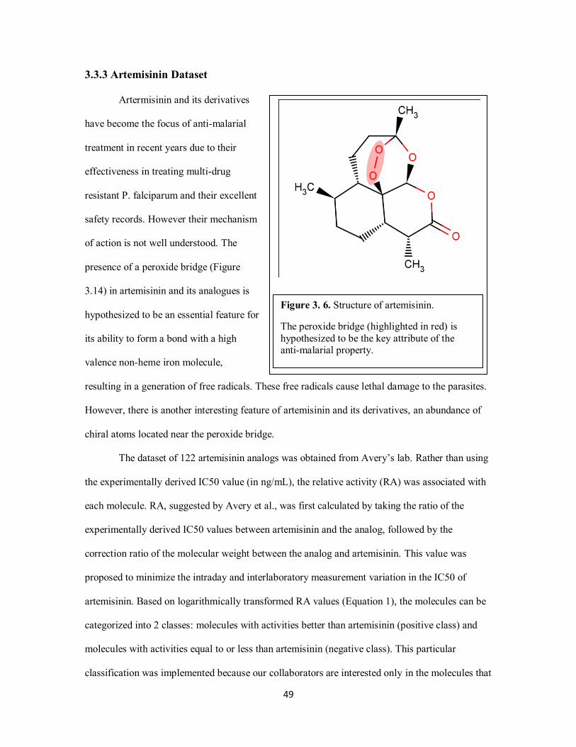
49

3.3.3 Artemisinin Dataset

Artermisinin and its derivatives

have become the focus of anti-malarial

treatment in recent years due to their

effectiveness in treating multi-drug

resistant P. falciparum and their excellent

safety records. However their mechanism

of action is not well understood. The

presence of a peroxide bridge (Figure

3.14) in artemisinin and its analogues is

hypothesized to be an essential feature for

its ability to form a bond with a high

valence non-heme iron molecule,

resulting in a generation of free radicals. These free radicals cause lethal damage to the parasites.

However, there is another interesting feature of artemisinin and its derivatives, an abundance of

chiral atoms located near the peroxide bridge.

The dataset of 122 artemisinin analogs was obtained from Avery’s lab. Rather than using

the experimentally derived IC50 value (in ng/mL), the relative activity (RA) was associated with

each molecule. RA, suggested by Avery et al., was first calculated by taking the ratio of the

experimentally derived IC50 values between artemisinin and the analog, followed by the

correction ratio of the molecular weight between the analog and artemisinin. This value was

proposed to minimize the intraday and interlaboratory measurement variation in the IC50 of

artemisinin. Based on logarithmically transformed RA values (Equation 1), the molecules can be

categorized into 2 classes: molecules with activities better than artemisinin (positive class) and

molecules with activities equal to or less than artemisinin (negative class). This particular

classification was implemented because our collaborators are interested only in the molecules that

Figure 3. 6. Structure of artemisinin.

The peroxide bridge (highlighted in red) is

hypothesized to be the key attribute of the anti-malarial property.

50

have activities better than artemisinin. As a result, the data contained 71 and 51entries associated

with positive and negative classes, respectively.

3.4 Evaluation of Descriptor Significance and Generalizability

Two different procedures were performed to evaluate the performance of the 3D chiral

atom-pair (cAP) descriptors. The first procedure was to evaluate the significances of different

cAP descriptor matrices, which were generated by varying the threshold for chirality. By varying

the chirality threshold, a different degree of chirality can be assigned to the corresponding cAP

descriptor matrix. This procedure allowed for the identification of a subset of chiral carbon atoms

that are more likely to attribute to a given biological target property by optimizing the chirality

threshold to achieve the highest model significance. The calculation of model significance

described in Section 2.3.1 was applied to the full dataset without data partitioning to identify the

optimal chirality threshold. By varying the chirality threshold from 0.001 to 0.029 with an

increment of 0.002, a total of fifteen cAP descriptor matrices were generated for each of the three

datasets. A regular atom-pair descriptor matrix (APair) without chiral atom types was generated

as a control group in order to compare the significance of the chiral atom types.

To evaluate the generalizability of the cAP descriptors, the five-fold external cross-

validation procedure described in Section 2.6 was applied to generate five different sets of

descriptor matrices for the performance benchmark. The benchmark was designed not only to

compare the performance between Dragon, APair, and cAP descriptors but also to evaluate the

potential for prediction accuracy by combining Dragon descriptors with chiral atom-pair

descriptors. Regular atom-pair descriptors were combined with Dragon descriptors to serve as a

control group in order to compare the generalizability of the chiral atom types in predicting

51

unseen data (data in the external test sets). All data entries in training and test sets remained the

same for the five different descriptor matrices.

3.5 Modeling Results

3.5.1 PEPT1 Dataset

Compared to all the fifteen cAP descriptor matrices, the model built with APair achieved

a much lower significance. As illustrated in Figure 3.7, all fifteen optimal models (models with

the highest z-scores) associated with the corresponding cAP descriptor matrices achieved much

Figure 3. 7. Degrees of chirality and the corresponding significance for the PEPT1 dataset.

The model significance, which is determined by the z-scores, indicated that models built

with the chiral atom types (atom types 16 and 17) were more significant than the model built

without (APair; black line). The most significant model was achieved with the threshold of 0.007 (cyan).

52

higher z-score values than the model with APair descriptors. This outcome indicated that the

chiral atom types do capture the effect of stereochemistry in this highly chirality sensitive dataset.

Additional comparison among the optimal models built with different cAP descriptors indicated

that different levels of significance were achieved by varying the chirality threshold (degree of

chirality). The observation of lower z-score values associated with thresholds ranging from 0.001

to 0.005 suggested the corresponding descriptor matrices contained some chiral atoms that might

be trivial to the target property. By considering those trivial chiral atoms as non-chiral atoms,

higher z-score values were obtained from the modified descriptor matrices, which were generated

by increasing the chiralty threshold. Given the ranges of chirality threshold evaluated in this study,

the highest z-score value was achieved by the optimal model obtained from the cAP descriptor

matrix with a chirality threshold of 0.007.

After establishing the association between the target property and the degree of chirality,

the next goal was to evaluate the generalizability of the 3D chiral atom-pair descriptors through a

five-fold external cross-validation procedure. To summarize the classification results for the five-

fold external cross-validation procedure, sensitivity, specificity, and CCR were calculated from

the single combined set of the five test sets associated with each descriptor matrix. The cAP

descriptor matrix being evaluated was generated with a threshold of 0.007. As illustrated in

Figure 3.8, the models obtained using cAP descriptors achieved higher prediction accuracy than

models obtained from either APair or Dragon descriptors alone. By combining Dragon and cAP

descriptors, the resulting optimal models achieved higher sensitivity, specificity, and CCR than

the models obtained from the combination of Dragon and APair descriptors. Furthermore, the

addition of either APair or cAP descriptors to Dragon descriptors improved the models prediction

accuracy more than the Dragon descriptors alone.

53

The benchmarking results of the five-fold external cross-validation indicated cAP

descriptors can be used to build predictive models, especially for a chirality sensitivity dataset. In

this PEPT1 dataset, models with cAP descriptors achieved more significance and higher

prediction accuracy than models with APair descriptors. Both cAP and APair descriptors encoded

valuable information associated with PEPT1 binding that is not captured by 2D descriptors such

as the Dragon descriptors.

Figure 3. 8. Five-fold external cross-validation results of the PEPT1 dataset.

Models built with descriptors containing only 2D molecular structure information (Dragon

descriptors) performed worse than models built with descriptors containing 3D molecular

structure information. Among the descriptors containing 3D molecular structure

information, descriptor matrices containing chiral atom pair descriptors yielded much

better performances in classifying the test sets.

54

3.5.2 AmpC β–lactamase Dataset (149 Compounds)

When compared to the APair descriptors, only the two cAP descriptor matrices generated

with the thresholds 0.011 and 0.013 achieved higher values in z-scores during the evaluation of

significance. As illustrated in Figure 3.9, most of the optimal models (models with the highest z-

score) associated with the corresponding cAP descriptor matrices achieved similar if not lower z-

score values than the model with APair descriptors. This outcome matched the fact that this

AmpC β-lactamase dataset is fairly insensitive to stereochemistry since there only existed a pair

of enantiomers with different property labels. However, the outcome of higher z-scores achieved

Figure 3. 9. Degrees of chirality and the corresponding significance for AmpC β-lactamase dataset (149 compounds).

The semi-log plot indicated that only the chiral atom pair descriptor matrices generated with a threshold of 0.011 and 0.013 were more significant than the regular atom pair descriptor

matrix (APair).

55

by setting the chirality threshold to 0.011 and 0.013 suggested that the targeted biological

property could be influenced by a subset of chiral atoms within the molecular entries. These

potentially influential chiral atoms and their associated 3D molecular patterns became less

distinctive as the chirality threshold further increased, thus resulting in a drop in z-score values.

A five-fold external cross-validation procedure was applied to evaluate the

generalizability of the cAP descriptors. To summarize the classification results for the five-fold

external cross-validation procedure, sensitivity, specificity, and CCR were calculated from the

single combined set of the five test sets associated with each descriptor matrix. The cAP

Figure 3. 10. Five-fold external cross-validation result of AmpC β-lactamase dataset (149

compounds).

For this AmpC β-lactamase dataset, the models built with chiral atom pair descriptors

achieved better specificity than models built with other descriptors. The outcome was

interesting, especially when comparing the model performance between descriptor

matrices containing chiral atom pair descriptors only and the combined descriptor matrix

containing both Dragon and chiral atom pair descriptors.

56

descriptor matrix being evaluated was generated with a threshold of 0.011. As illustrated in

Figure 3.10, the models obtained using cAP descriptors achieved higher prediction accuracy

(higher specificity) than models obtained from either APair or Dragon descriptors alone.

However, the difference in performance only existed when predicting the non-inhibitors. The

combination of Dragon descriptors with either APair or cAP descriptors showed minor

performance gain in specificity more than the Dragon descriptors alone. However, combining

Dragon and cAP descriptors achieved similar if not equivalent results to the combination of

Dragon with APair descriptors.

The benchmarking results of the five-fold external cross-validation indicated cAP

descriptors can be used to build predictive models that are comparable to the models built with

Dragon descriptors. For this AmpC β-lactamase dataset, which is relative insensitive to

stereochemistry, models built with cAP descriptors achieved higher prediction accuracy than

models with other descriptors. Given the higher prediction accuracy associated with models built

with cAP and APair descriptors, there could be molecular patterns encoded in these descriptor

matrices that might not be captured by 2D descriptors such as the Dragon descriptors.

3.5.3 Artemisinin Dataset

Similar to the PEPT1 dataset, the model built with APair achieved a much lower

significance when comparing all fifteen cAP descriptor matrices. As illustrated in Figure 3.11, all

fifteen optimal models (models with the highest z-scores) associated with the corresponding cAP

descriptor matrices achieved much higher z-score values than the model with APair descriptors.

This outcome indicated that the chiral atom types do capture the effect of stereochemistry in this

chirality sensitive dataset. Additional comparison among the optimal models built with different

cAP descriptors indicated that different levels of significance were achieved by varying the

chirality threshold (degree of chirality). Given the ranges of chirality threshold evaluated in this

57

study, the highest z-score value was achieved by the optimal model obtained from the cAP

descriptor matrix with a chirality threshold of 0.015.

Five-fold external cross-validation was applied to evaluating the generalizability of the

3D chiral atom-pair descriptors. To summarize the classification results from the five-fold

external cross-validation procedure, average values for sensitivity, specificity, and CCR were

reported for each descriptor matrix. The cAP descriptor matrix being evaluated was generated

with a threshold of 0.015. As illustrated in Figure 3.12, the models obtained using cAP

Figure 3. 11. Degrees of chirality and corresponding significance for the artemisinin dataset.

The model significance, which is determined by the z-scores, indicated that models built

with the chiral atom types (atom types 16 and 17) were more significant than the model built

without (APair; black line). The most significant model was achieved with the threshold of

0.015(red).

58

descriptors achieved higher CCR than models obtained from either APair or Dragon descriptors

alone. By combining Dragon and cAP descriptors, the resulting optimal models achieved higher

specificity than the models obtained from the combination of Dragon and APair descriptors. With

the addition of either APair or cAP descriptors combined with Dragon descriptors, the prediction

accuracy of the models improved compared to models obtained from Dragon descriptors alone.

The benchmarking results of the five-fold external cross-validation indicated that cAP

descriptors can be used to build predictive models for datasets containing chiral centers but not

necessarily including enantiomeric pairs. In this artemisinin dataset, models with cAP descriptors

Figure 3. 12. Five-fold external cross-validation result of the artemisinin dataset.

For this, the models built with chiral atom pair descriptors achieved better specificity than

models built with other descriptors. Similar to the outcome obtained from the AmpC β-

lactamase dataset, models built with chiral atom pair descriptors only achieved better

specificity than the combined descriptor matrix containing both Dragon and chiral atom

pair descriptors.

59

achieved more significance and higher prediction accuracy than models with APair descriptors.

Both cAP and APair descriptors encoded valuable information associated with antimalarial

property that is not captured by the 2D descriptors, such as the Dragon descriptors

3.6 Conclusion

Chirality is an important concept in medicinal chemistry, and many biochemical reactions

and processes are stereospecific, such as the recognition of ligands by their corresponding

receptors. In order to identify key stereochemistry associated with a given biological property,

novel 3D chiral atom-pair descriptors were developed. By varying the chirality threshold,

different subsets of chiral atoms and their associated molecular patterns were encoded in a

descriptor matrix. Three datasets containing stereochemistry information were selected for

benchmarking the developed descriptors. Results indicated that the models based on developed

3D chiral atom-pair descriptors were more predictive than models obtained from non-chiral 3D

atom-pair or 2D Dragon descriptors alone. The difference in descriptor performance directly

correlated to the amount of stereochemistry information available in the dataset.

Due to the varying amount of chirality data available in the datasets, both 3D chiral and

3D non-chiral atom-pair descriptors were independently compared in combination with 2D

Dragon descriptors. The resulting models indicated better prediction accuracy than models

obtained from Dragon descriptors alone, suggesting that the 3D atom-pair descriptors used in this

study could be complementary to Dragon descriptors. However, lower prediction accuracy

associated with the models obtained from both sets of combined descriptors (Dragon + 3D atom-

pairs) when compared to models obtained from 3D atom-pair descriptors alone raised two

concerns: 1) a problem of simple merge for descriptor matrices and 2) a limitation of DWD with

variable selection. Thus, simple merging of descriptor matrices can result in the united descriptor

matrix containing highly correlated descriptors, which could affect the descriptor loadings

assigned in DWD and decrease the predictivity of the resulting model. To address this problem

60

and to improve the performance of the variable selection DWD, correlation between descriptors

will have to be considered as part of the variable selection procedure. One possible method would

be to cluster the descriptors first and evaluate the significance of the descriptors as a group. This

solution will likely retain all instances when important descriptors are highly correlated with one

another.

Chapter 4

Novel Protein Descriptors

4.1 Growth of Protein Structure Data

Proteins, whether from bacteria or the most complex forms of life, are constructed from

the same ubiquitous set of twenty amino acids (building blocks). Cells can produce proteins with

strikingly different properties and activities by joining these building blocks in many different

combinations and varying the length of sequences, creating a great variety of enzymes with

specific biological activities. Enzymes are usually very specific to the reactions they catalyze and

the substrates involved. Impressive levels of stereo-, region- and chemo-specificity have been

demonstrated in enzymes 71

. This specificity is achieved by the complementarity in characteristics

such as shape, charge and pattern of hydrophilic/hydrophobic interactions between enzymes and

substrates.

Enzymes are generally globular proteins made of long, linear chains of amino acids that

fold to three-dimensional structures with their sizes ranging from 62 amino acid residues, e.g., the

monomer of 4-oxalocrotonate tautomerase 35

, to over 2,500 residues, e.g., the fatty acid synthase

found in animals 123

. Each unique amino acid sequence produces a specific structure, which has

unique properties. Individual protein chains may sometimes group together to form a protein

complex. Most enzymes are much larger than the substrates they act on, but only a small portion

of the enzyme (up to 7 amino acids) is believed to be directly involved in catalysis 15

. This region,

which is responsible for binding the substrate and carries out the reaction, is known as the active

site. Enzymes can also contain sites (allosteric sites) that bind cofactors (for catalysis) and/or

small molecules that directly or indirectly interact with products or substrates of the reaction

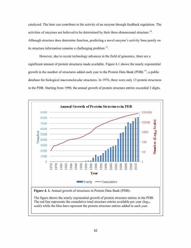
62

catalyzed. The later can contribute to the activity of an enzyme through feedback regulation. The

activities of enzymes are believed to be determined by their three-dimensional structure 10

.

Although structure does determine function, predicting a novel enzyme’s activity base purely on

its structure information remains a challenging problem 51

.

However, due to recent technology advances in the field of genomics, there are a

significant amount of protein structures made available. Figure 4.1 shows the nearly exponential

growth in the number of structures added each year to the Protein Data Bank (PDB) 19

, a public

database for biological macromolecular structures. In 1976, there were only 13 protein structures

in the PDB. Starting from 1990, the annual growth of protein structure entries exceeded 3 digits.

Figure 4. 1. Annual growth of structures in Protein Data Bank (PDB).

The figure shows the nearly exponential growth of protein structure entries in the PDB. The red line represents the cumulative total structure entries available per year (log10

scale) while the blue bars represent the protein structure entries added in each year.

63

Beginning with 1993, the pace at which protein structures are being discovered has grown at a

much faster rate, with the PDB exceeding 23,000 structures in 2003, and 78,000 in 2011.

With the increase in protein structure entries, the number of protein structures with

unknown function also increases. There were only 5 protein structures with unknown function in

2000, but within a decade, that number had quickly grown to 2,422. Figure 4.2 illustrates the

number of protein structures obtained by querying 110

with the keyword, “Unknown_Function,”

grouped by the year that the structure was released. Identifying the function of these protein

structures remains a challenging task.

A recent revision 110

of the PDB allows users easier retrieval of protein structure entries

based on a wide variety of information associated with the entries. Possible query types include,

but are not limited to, structure features, sequence features, chemical components, biology, and

method. Under the biology query types, users can retrieve protein structure entries with similar

Figure 4. 2. Annual growth of protein structures with unknown function.

64

functions by querying Enzyme Commission or Classification (E.C.) number, which is a numerical

classification scheme for enzymes that is based on the chemical reactions they catalyze. The E.C.

number is based on a hierarchical order as denoted by the four numbers separated by periods,

with the first number ranging from one to six to represent the six major classes of enzyme:

oxidoreductases (E.C. 1), transferases (E.C. 2), hydrolases (E.C. 3), lyases (E.C. 4), isomerases

(E.C. 5), and ligases (E.C. 6). As the notations increase in length, a progressively finer

classification of the enzyme can be obtained. The first version of the enzyme classification

number, which contains 712 enzymes, was published in 1961. The latest version, published in

1992, contains 3,196 different enzymes 1.

4.2 Overview of Current Methods for Protein Function Annotation

Function-prediction methods existing today are based on the sequence-function and

structure-function relationships of proteins. The challenge for protein function annotation is to

decipher the connection between the structural or sequence similarities and the actual level of

functional relatedness. In this section, we describe the progress in the automated prediction of

protein function based on protein sequence and structure. We will first focus on methods that

attempt to extract functional information from protein sequences, which generally utilize

sequence alignment and clustering, and then discuss methods that use protein structure

information.

4.2.1 Sequence-Based Methods

Sequence-based methods annotate protein structures with possible function by either

grouping proteins into families or comparing a target sequence with pre-compiled databases of

families, which often rely on a sequence similarity search through BLAST 8, or Basic Local

Alignment Search Tool. BLAST calculates similarity of a query sequence against a database of

sequences and retrieves sequences that resemble the query sequence above a certain threshold.

Sequences retrieved from BLAST are typically close homologues to the query sequence.

65

To identify distant homologues, Position-Specific Iterative BLAST, or PSI-BLAST 9, is

utilized. PSI-BLAST first retrieves a list of all closely related proteins and generates a sequence

profile based on multiple sequence alignment (MSA). This sequence profile, which summarizes

significant features presented in these closely related sequences, is served as query for searching

the database. Examples of these sequence profiles can be found at Conserved Domains Database

90 (CDD), ProDom

27, and PROSITE

68. Sequence profiles can also be obtained through hidden

Markov models (HMM), which assume the system being modeled is a memoryless stochastic

process with unobserved states. Examples of sequence profiles generated from HMM are

provided by Pfam 54

, EVEREST 106

, and SMART 85

. All profile-based methods vary significantly

in their level of automation, manual curation, and reliance on complementary resources in the

annotation of protein functions 88

. By integrating all the different methods, a more comprehensive

coverage can be achieved, such as shown in InterPro 95

, an integrated database of protein families

that combines at least twelve member databases.

4.2.2 Structure-Based Methods

Observations have been made that evolution retains the protein folding pattern long after

sequence similarity becomes undetectable 37;143

. For example, the catalytic triad located in the

active site of the enzyme is structurally preserved in all serine protease enzymes. The triad is a

coordinated structure consisting of three essential amino acids: histidine (His), aspartic acid (Asp),

and serine (Ser). Mapping the triad back to the sequence indicates that the His, Asp, and Ser are

located at sequence positions of 57, 102, and 195 for bacterial serine protease. For mammalian

serine protease, the positions are 64, 32 and 221 respectively (Figure 4.3). Neither the order nor

the length between these three amino acids is conserved at the sequence level 103

. Consequently, a

benchmark study showed that structural similarities can be more reliable than sequence

similarities for grouping proteins with a common biological function 88;131

.

66

Structure similarity can be calculated by using global structure comparison, which

compares the structure of a queried protein to domains in the structure databases. Global

structure-comparison methods, such as DALI 65

, MSDFold 79

, VAST 89

, CE 119

, STRUCTAL 73

,

and FATCAT 147

, identify structural neighbors in the Protein Data Bank through pairwise

structural alignment and differ in alignment methods; however, they do not discriminate between

conservation of the overall fold and functionally relevant regions of the protein 88

. By focusing

structure similarity comparison on more localized regions, such as clefts, pockets and surfaces,

the identification and comparison of such regions can suggest similarity in protein function,

because the ligand-binding pocket or active site is commonly situated in the largest cleft in the

protein 83

.

Multiple methods have been developed to define these local regions within a protein

structure. SURFNET 58;82

attempts to identify clefts by fitting spheres of a range of sizes between

atoms of a given protein. Further enhancement can be made by coupling SURFNET with

ConSurf 81

to isolate the clefts that are close in proximity to the evolutionarily conserved residues

which are defined by the ConSurfHSSP database 59

.

A surface-comparison method that identifies similar surface patterns based on

geometrically defined pocket and void surfaces of amino acid residues on proteins is called

pvSOAR 21;22

(pocket and void Surfaces Of Amino acid Residues). This method first establishes a

residue correspondence between surfaces by aligning sub-sequences of surface residues. These

residues are then superimposed and the resulting root-mean-square deviation (RMSD) is

evaluated for statistical significance. The pvSOAR and CASTp 52

databases are the two essential

components for the Global Protein Surface Survey (GPSS) 23

, which contains three-dimensional

libraries of functionally annotated surfaces from ligand, deoxyribonucleic acid (DNA), metal and

peptide binding surfaces.

Other methods such as Catalytic Site Atlas 105

, PDBSiteScan 69

, PINTS 124

(Patterns In

Non-homogous Tertiary Structures), and ET 87

(Evolutionary Trace) are template-based methods

67

to identify active-site residues. These methods utilize a variety of template-based scans to identify

active sites and putative ligand-binding pockets. The representation of a template varies by

method and can be derived either manually or automatically. For Catalytic Site Atlas, the

templates can either reflect the backbone orientation (a set of Cα and Cβ atoms) or the orientation

of the ends of the residue sidechains (three functional atoms for each sidechain). These templates

from Catalytic Site Atlas are derived manually by mining the literature. The templates from

PDBScan that contain a set of residues and their corresponding atoms are automatically generated

based on the information within the SITE records of PDB files and protein-protein interaction

data. PINTS defines its templates by detecting the largest common 3D arrangement of residues

between any two structures. The representation of the templates in PINTS can be atoms or points

defined by other criteria (e.g., sidechain centroids). As for ET, it uses phylogenetic trees to rank

residues in a protein sequence by their evolutionary importance and maps these residues onto the

structure.

There are also other pocket-centric methods, such as FEATURE 12

, SiteEngine 121

, and

SURF’S UP 116

, that describe protein-ligand interactions and active-site chemistry by the

physicochemical properties of the local environments in the pockets and surfaces. For example,

FEATURE represents the local microenvironment using various physical and chemical properties

ranging from simple atom-based characteristics such as charge to polypeptide-based

characteristics such as type of secondary structure. These methods are based on the assumption

that protein surface regions with similar physicochemical properties and shapes may perform

similar functions and bind similar binding partners.

Integrating multiple resources from both sequence-based and structure-based methods

provides a consensus view, which increases the likelihood of accurate predictions of function.

Examples of such integrated metaservers include ProFunc 84

and ProKnow 102

. However, most

methods described above either rely on global structural alignment or local region comparison

(template based). Methods based on global structural alignment find proteins with a similar fold,

68

but will not be successful when either proteins adopt a new fold (i.e., does not resemble any

known structure) or proteins adopt very common folds that perform many different functions.

Template-based methods usually perform better in scenarios where methods based on global

structural alignment fail; however, the performance of the template-based methods depends on

the identification of the active sites.

4.3 Motivation

With the large amount of protein structure information available, identifying the common

structure features, or structure motifs associated with a group of enzymes sharing similar

functions, has become feasible. Once identified, the presence of these structure motifs, which

could be portions of an active site, allosteric site, or structure conserved region, is used to

associate (or infer) the protein structures with unknown functions to a enzyme class with known

function. Function inference from structure is facilitated by the use of patterns of residues (3D

motifs), normally identified by expert knowledge, that correlate with function. As an alternative

to often limited expert knowledge, we use statistical learning techniques and novel protein

descriptors to automatically identify residues that contribute to protein functions.

4.4 Novel Protein Descriptors

The goal for designing novel protein descriptors is to study the structure-function

relationship of proteins through QSAR-like strategies. By combining variable selection DWD

with the novel protein descriptors, it is possible to identify important amino acids that are

common in proteins with similar functions.

The novel protein descriptors implemented in this research are designed to characterize

the three-dimensional protein structures, with emphasis on the local geometric properties of

proteins. The rationale is that the 3D arrangement of enzyme active-site residues is often more

conserved than the overall fold. For enzymes, or proteins with similar functions, it is not the

similarity of their global structures that define their functions but rather the catalytic sites (local

69

region). Enzymes can have dissimilar structures globally but perform the same catalytic reaction.

The goal of this set of descriptors is to capture the information within the local regions of protein

structures.

For protein function annotation, multiple studies have successfully identified family

motifs by applying Delaunay Tessellation to the protein crystal structures 33;67;78;118;122;135;137-139

. By

representing amino acid residues in protein chains by Cα atoms or side-chain centroids, a protein

is represented as a set of points in three-dimensional space. Cα atoms, which are located on a

protein backbone, were chosen to represent the amino acid residues in the protein descriptors for

their relative stability over the side-chain centroid. Delaunay Tessellation naturally partitions the

space occupied by the protein into tetrahedra with Cα atoms or side-chain centroids at their

vertices. Implementing Delaunay tessellation on this set of points generated an aggregate of

space-filling irregular tetrahedra, or Delaunay simplices. The vertices of each simplex

(tetrahedron) define objectively four nearest neighbor Cα atoms, which correspond to four

nearest-neighbor residues; thus, these tetrahedra can be categorized by the amino acid residues

occupied at their vertices. By combining the different categories of tetrahedra and the

corresponding geometric properties, a protein structure can be encoded as a feature vector.

4.4.1 Classification Scheme of Amino Acids (Ten Classes) and Geometric Properties

Each tetrahedron is categorized by the various amino acids occupied at its four vertices,

and the number of possible tetrahedral categories, if determined by all the twenty amino acids, is

8,855. This number is tripled when geometric features, such as volume, exposed surface area, and

hidden surface area, are incorporated into each tetrahedral category as features to describe protein

structures. This rapid increase in dimensions puts constraints on the number of possible geometric

properties that can be incorporated into each tetrahedral category. By reducing the twenty amino

acids labels into ten classes, the total number of tetrahedral categories can be drastically reduced

(a reduction that exceeds tenfold reduction), and Table 4.1 showed the categorization of possible

70

tetrahedral associated with twenty amino

acids and ten amino acid classes, which

are 8,855 and 715 respectively. A recent

study by Li et al. compared the ability to

detect distantly related protein folds with

various reduced alphabets of amino acids

and suggested that ten classes of amino

acids may be the degree of freedom for

characterizing the complexity in proteins 86

.

We assigned the vertices of the tetrahedra

using a modified Delvin’s amino acid

classification (Table 4.2) that classifies

twenty amino acids into ten classes.

After establishing the tetrahedral categories with ten amino acid classes, we calculated

various geometric properties, such as volume and two different surface area measures (i.e.,

hidden and exposed surfaces between tetrahedra), for a set of tetrahedra to describe a protein

structure. The volume of a tetrahedron encodes the proximity of the four amino acids at its

vertices situated in space. The hidden surface area is the surface area that a tetrahedron shared

with its nearest neighboring tetrahedron, and the exposed surface area is the unshared surface area

of a tetrahedra. By recording different surface area measures, the location of the tetrahedron with

respect to other tetrahedra was encoded in the descriptors. For instance, a tetrahedron surrounded

by 4 other tetrahedra would have zero exposed surface area; thus it is buried inside the protein

structure.

Tetrahedral Qty Qty

Categories (20 amino acids) (10 Classes)

AAAA 20 10

AAAB 380 90

AABB 190 45

AABC 3420 360

ABCD 4845 210

Total 8855 715

Table 4. 1. Possible categories of tetrahedra.

The amino acids corresponding to the

vertices of each tetrahedron can be classified

into 10 classes. By placing the twenty amino

acids into ten classes, there is a reduction of

the possible tetrahedron types from 8,855 to

715. The A, B, C, and D, which are listed in

the tetrahedral categories, represent different

labels or classes of amino acids.

71

Our implemented protein descriptors characterize a protein structure with a vector

containing 2,145 features, which include the total volume, total hidden surface area, and total

exposed surface area for each of the 715 tetrahedral categories. As illustrated in Figure 4.3, when

comparing two hypothetical proteins containing the same amount of tetrahedra of the same

category but different sizes, one can easily distinguish the two proteins by using the total volume.

Class Full Name 3 Letter 1 Letter Superstructure structure

Glycine Gly G

Alanine Ala A

Valine Val V

Leucine Leu L

Isoleucine Ile I

2 Proline Pro P Monoamino, monocarboxylic Heterocyclic

Tyrosine Tyr Y

Phenylalanine Phe F

Tryptophan Trp W

4 Methionine Met M Monoamino, monocarboxylic Thioether

Serine Ser S

Threonine Thr T

6 Cysteine Cys C Monoamino, monocarboxylic Mercapto

Asparagine Asn N

Glutamine Gln Q

Aspartate Asp D

Glutamate Glu E

Lysine Lys K

Arginine Arg R

Histidine His H

Small

Unsubstituted

Aromatic

Hydroxy

Carboxamide

8

9

Monoamino, monocarboxylic





Monoamino, dicarboxylic

Diamino, monocarboxylic

1

0

3

5

7

Table 4. 2. Classification of amino acids.

The twenty amino acids were partitioned into 10 classes based on Devlin46

. We

split Class 0 and Class 1, which Devlin puts in the same class.

72

4.4.2 Geometric Property of α–helix vs. β sheet

In proteins, α–helix and β-sheet are the two common forms of secondary structure, or

highly regular local sub-structures. To evaluate the ability of different geometric properties in

capturing the difference between α–helix and β-sheet, we applied Delaunay Tessellation to Cα

atoms of two PDB entries that represent α–helix (PDB ID: 2GOF) and β-sheet (PDB ID: 2JNI).

We then removed tetrahedra containing an edge greater or equal to 12 Å in order to focus on the

local neighborhood relationships of amino acids within a protein structure. Setting the threshold

to 12 Å was empirical, and this threshold value was determined based on tessellating a random

set of PDB entries to avoid orphan Cα atoms that were not associated with any tetrahedron.

Visual comparison between the two sets of Delaunay simplices (tetrahedra) suggested that

15 14 13

Protein B

40 28

19

Protein A

Figure 4. 3. Illustration of the potential benefit by encoding the geometric property of

tetrahedra for proteins.

Both protein A and B contain three instances of a particular tetrahedral category with

different sizes. Based on the instances of the tetrahedral category, the two proteins are

indistinguishable, but the two proteins become distinguishable when total volume is used

to characterize these tetrahedra within the two proteins.

73

geometric properties alone (without information regarding the composition of amino acids) can

distinguish α–helix from β sheet. Figure 4.4 indicates that the packing of tetrahedra between α–

helix (PDB ID: 2GOF) and β-sheet (PDB ID: 2JNI) appears different. The tetrahedra in α–helix

visually appear more uniform than those in β sheet.

By comparing three geometric properties of tetrahedra, i.e., volume, hidden surface area,

and exposed surface area, between α–helix and β-sheet, we can make two observations. First, the

tetrahedra associated with α–helix have less variation in both volume and hidden surface area

(shared surface area). The tetrahedra with volume greater than 15 units or with exposed surface

area greater than 60 units were likely to belong to β sheet. This result confirmed the uniformity of

tetrahedra associated with α–helix that were previously observed through visual inspection.

Second, the exposed surface areas for tetrahedra associated with both α–helix and β-sheet

have a similar longtail distribution with zero as the dominate value (bottom plot of Figure 4.5).

This finding suggested that using the exposed surface area of a tetrahedron as a feature by itself is

insufficient to distinguish an α-helix from a β sheet.

Figure 4. 4. α–helix vs. β–sheet.

The packing of the tetrahedra in blue and red corresponds to the α–helix (PDB ID: 2GOF) and the β-sheet (PDB ID: 2JNI) respectively. The tetrahedra in α–helix are more uniform

in size than those in β-sheet.

74

Figure 4. 5. Difference in geometric properties of tetrahedra between α-helix and β sheet.

Tetrahedra associated with α-helix are blue; those with β-sheet are red. The tetrahedra

associated with α-helix are more uniform than those from β-sheet as shown in volume (top) and hidden surface area (middle). It is less distinctive in exposed surface area (below).

75

4.5 Selection of Enzyme Diversity Set

We selected a subset representing each of the six major types of enzyme as the enzyme

diversity set. This enzyme diversity set served as the negative class to contrast with the enzyme

class of interest (positive class) in order for the classifier described in Chapter 2 to extract

tetrahera unique to the positive class. The selection criteria for PDB entries associated with each

major enzyme type were as follows:

Must be a biological unit

Must match the enzyme classification number (top level)

Must have X-ray resolution better than 1.59 Å

Must have sequence identity less than 50%

Figure 4. 6. Distribution of the six major enzyme groups in the enzyme diversity set.

There are 1,005 enzymes in the enzyme diversity set, consisting of hydrolases (EC 3) 45%, transferases (EC 2) 21%, and oxidoreductases (EC 1) 18%. Lyases (EC 4),

isomerases (EC 5), and ligases (EC 6) made up the remaining data, each less than 10%.

76

The resulting enzyme diversity set contained 1,005 PDB entries, consisting of hydrolases (EC 3)

45%, Transferases (EC 2) 21%, and oxidoreductases (EC 1) 18%. Lyases (EC 4), isomerases (EC

5), and ligases (EC 6) made up the remaining data, with each less than 10%. Figure 4.6 shows the

distribution of enzyme families in the enzyme diversity set. The number of entries in the enzyme

diversity set was further reduced by removing entries with identical function as the enzyme class

of interest. Thus the size of the enzyme diversity set depends on the enzyme class of interest.

The distribution of the enzyme families within the enzyme diversity set showed the

limitation for selecting the enzyme class of interest. With the data size of isomerases and ligases

both under 50, it was not feasible to study the enzymes in these two groups with more specific

function.

4.6 Selection of Enzyme Homologs

The level of function specificity for a given enzyme class can be determined by its EC

number. The length of the EC numbers (up to four digits) is designed to reflect the level of

specificity in enzyme function. As the enzyme functions become more specific, their

corresponding EC number becomes longer. The selection criteria for the enzyme homologs were

similar to that of the enzyme diversity set. However, the sequence identity criterion had to be

modified in order to obtain a sufficient number of structure entries that are functional homologs

with low sequence similarity. The selection criteria for the enzyme homologs were as follows:

Must be a biological unit

Must match exactly the enzyme classification number

Must have X-ray resolution better than 1.59 Å

Must have sequence identity less than 70%

The PDB partitions the sequence identity into intervals and the jump from 50% to 70% is the

smallest step possible. Six different functional classes of enzyme homologs were selected

according to these criteria: superoxide dismutase (EC1.15.1.1), cellulase (EC 3.2.1.4), β-

77

lactamase (EC 3.5.2.6), methyltransferase (EC 2.1.1), protein-tyrosine kinase (EC 2.7.10), and

protein-serine/threonine kinases (EC 2.7.11).

These six functional classes of enzyme homologs were selected because the numbers of

entries associated with them are sufficient after applying the selection criteria. More than ten

PDB entries, which are functional homologs, were retrieved for all of the six enzyme classes.

These six enzyme classes could be grouped into two types: enzymes classes with more specific

function or enzymes classes with more general functions. The goal to include enzyme classes

with two different levels of function specificity was to evaluate the capability of applying the

protein descriptors in order to study enzyme classes with more generalized function.

4.6.1 Superoxide Dismutase (EC 1.15.1.1)

EC 1.15.1.1 is the enzyme classification number for superoxide dismutases (SOD). The

enzymes that belong to this class are responsible to catalyze the dismutation of superoxide into

oxygen and hydrogen peroxide. They serve as an important antioxidant defense in nearly all cells

exposed to oxygen. Three

major families of

superoxide dismutase are

classified based on the

binding metal cofactor:

SODs that bind to nickel,

SODs that bind to either

iron or manganese, and

SODs that bind to

copper/zinc.

Abnormalities in the

copper- and zinc-

PDB Entries Types

1BSM IRON (III) SUPEROXIDE DISMUTASE

1F1G COPPER,ZINC SUPEROXIDE DISMUTASE

1IX9 MANGANESE SUPEROXIDE DISMUTASE

1MFM COPPER,ZINC SUPEROXIDE DISMUTASE

1OAL COPPER,ZINC SUPEROXIDE DISMUTASE

1T6U NICKEL SUPEROXIDE DISMUTASE

1TO4 COPPER,ZINC SUPEROXIDE DISMUTASE

1XSO COPPER,ZINC SUPEROXIDE DISMUTASE

2AQM COPPER,ZINC SUPEROXIDE DISMUTASE

2AQP COPPER,ZINC SUPEROXIDE DISMUTASE

2NYB IRON (II) SUPEROXIDE DISMUTASE

2P4K MANGANESE SUPEROXIDE DISMUTASE

3CE1 COPPER,ZINC SUPEROXIDE DISMUTASE

3F7L COPPER,ZINC SUPEROXIDE DISMUTASE

Table 4. 3. Fourteen PDB entries retrieved based on the selection criteria from EC 1.15.1.1.

78

dependent superoxide dismutase gene may contribute to the development of Amyotrophic Lateral

Sclerosis, a fatal disease that causes deterioration of motor nerve cells in the brain and spinal cord

41;98;109. Table 4.3 shows the fourteen PDB entries associated with SOD that met the selection

criteria.

4.6.2 Cellulase (EC 3.2.1.4)

EC 3.2.1.4 is the enzyme classification number for cellulase, which is a class of enzymes

produced by fungi, bacteria, and protozoans to catalyze cellulolysis. Other types of organisms,

including some plants and animals, also produce cellulases. Several different kinds of cellulases

are known, which differ structurally and mechanistically, and their applications exist in both

commercial and pharmaceutical settings. Commercial applications of cellulases include laundry

detergents; food processing, e.g., hydrolysis of cellulose during drying of coffee beans; and

renewable energy, e.g., hydrolysis of cellulose in biomass to glucose in the fermentation stage.

Since cellulase is a digestive

enzyme and an anti-cholinergic

agent, it is used to help digest

protein, starch, and fat. As a result,

there are also pharmaceutical

applications associated with

cellulases, including treatments for

bowel spasms and Phytobezoars, a

form of cellulose bezoar found in

the human stomach. Table 4.4

shows the eighteen retrieved PDB

entries associated with cellulase

based on the selection criteria.

PDB Entries Types

1H1N ENDO TYPE CELLULASE ENGI

1KS8 ENDO-BETA-1,4-GLUCANASE

1KWF ENDOGLUCANASE A

1OA2 ENDO-BETA-1,4-GLUCANASE

1OJJ ENDOGLUCANASE I

1OLR ENDO-BETA-1,4-GLUCANASE

1TVN CELLULASE

1UWW ENDOGLUCANASE

1WC2 ENDOGLUCANASE

2BOG ENDOGLUCANASE E-2

2BW8 ENDOGLUCANASE

2E4T ENDOGLUCANASE

2ENG ENDOGLUCANASE V

2JEN ENDO-BETA-1,4-GLUCANASE

2NLR ENDOGLUCANASE

2V3G ENDOGLUCANASE H

3ACH ENDO-BETA-1,4-GLUCANASE

7A3H ENDOGLUCANASE

Table 4. 4. Eighteen PDB entries retrieved based on

the selection criteria for EC 3.2.1.4.

79

4.6.3 β-lactamase (EC 3.5.2.6)

EC 3.5.2.6 is the enzyme classification number for β-lactamase, which is secreted by

Gram-negative bacteria to hydrolyze the β-lactam ring of penicillins and cephalosporins. Based

on the specificity of the β-lactamase, individual enzymes may be called penicillinase or

cephalosporinase. There are four groups of β-lactamase that are roughly determined by inhibition

of clavulanic acid. Enzymes in group 1 are cephalosporinases not inhibited by clavulanic acid

while enzymes in group 4 are penicillinases that are also not inhibited by clavulanic acid. Group 2

contains penicillinases, cephalosporinases, or both that are inhibited by clavulanic acid. Group 3

holds the zinc based or metallo β-lactamases. Due to the increased size in group 2, it can further

be divided into 8

subgroups based

on the specificity

of the enzymes.

Table 4.5 showed

the twelve

retrieved PDB

entries associated

with β-lactamase

based on the

selection criteria.

PDB Entries Types

1K38 BETA-LACTAMASE OXA-2

1K55 BETA-LACTAMASE OXA-10

1M2X CLASS B CARBAPENEMASE BLAB-1

1M6K BETA-LACTAMASE OXA-1

1MQO BETA-LACTAMASE II

1NYM BETA-LACTAMASE TEM

1O7E L2 BETA-LACTAMASE

1ONG BETA-LACTAMASE SHV-1

1ZKJ EXTENDED-SPECTRUM BETA-LACTAMASE

2GMN METALLO-BETA-LACTAMASE

2HDS BETA-LACTAMASE

3G35 BETA-LACTAMASE CTX-M9A

Table 4. 5. Twelve PDB entries retrieved based on the selection

criteria for EC 3.5.2.6.

80

4.6.4 Methyltransferases (EC 2.1.1)

A methyltransferase (EC 2.1.1) is a type of

transferase enzyme that transfers a methyl group from a

donor to an acceptor and can be further classified into

195 subfamilies. Methylation often occurs on amino

acids in protein structures or nucleic bases in DNA.

DNA methylation is often utilized to silence and regulate

genes without changing the original DNA sequence.

While DNA methylation is an important regulator of

gene transcription, its role in carcinogenesis has recently

generated considerable interest 43

. Compared with

normal cells, the malignant cells show major disruptions

in their DNA methylation patterns 17;18;43

.

Methylation of amino acids in the formation of

proteins leads to more diversity of possible amino acids

and, therefore, more diversity of function. The

methylation reactions occurring on nitrogen atoms in N-

terminal and side-chain positions are generally

irreversible 38;39

. Table 4.6 shows the thirty-two retrieved

PDB entries associated with methyltransferase based on

the selection criteria.

PDB Entries E.C. Numbers

1EJ0 2.1.1.-

1I1N 2.1.1.77

1JG1 2.1.1.77

1NTH 2.1.1.-

1V2X 2.1.1.34

2BLN 2.1.1.2

2F69 2.1.1.43

2G8O 2.1.1.45

2GB4 2.1.1.67

2NXC 2.1.1.-

2WK1 2.1.1.-

2Z6R 2.1.1.98

3AJD 2.1.1.-

3BO5 2.1.1.43

3C3Y 2.1.1.104

3CJS 2.1.1.-

3CKK 2.1.1.33

3DMG 2.1.1.-

3DOU 2.1.1.-

3DUW 2.1.1.-

3DXY 2.1.1.33

3EVF 2.1.1.56;2.7.7.48

3F9X 2.1.1.43

3FRH 2.1.1.-

3FTD 2.1.1.-

3FUT 2.1.1.-

3G5S 2.1.1.74

3G5T 2.1.1.145

3G89 2.1.1.-

3HNA 2.1.1.43

3HVI 2.1.1.6

3M6W 2.1.1.-

Table 4. 6. Thirty-two PDB

entries retrieved based on the

selection criteria for EC 2.1.1.

81

4.6.5 Protein-Tyrosine Kinases (EC 2.7.10)

Tyrosine kinase is an enzyme that regulates many cellular functions through the transfer

of a phosphate group from adenosine-5’-triphosphate (ATP) to the amino acid tyrosine on the

protein. Phosphorylation of proteins by kinases is an important mechanism in cellular signal

transduction and cellular activity regulation in response to external and internal stimuli. The

cellular activities regulated by tyrosine kinases include apoptosis, cell cycle progression,

cytoskeletal rearrangement, differentiation, development, the immune response, nervous system

function, and transcription 111

. Dysregulation of protein kinases caused by the mutation or the

fusion of tyrosine kinases with a partner protein has been implicated with cancer 77;111

.

Protein tyrosine kinases are divided into two

main classes: receptor tyrosine kinases (EC 2.7.10.1)

and nonreceptor tyrosine kinases (EC 2.7.10.2). Both

receptor and nonreceptor tyrosine kinases have emerged

as clinically useful drug target molecules for treating

certain types of cancer 77;141

. Table 4.7 shows the eleven

retrieved PDB entries associated with EC 2.7.10 based

on the selection criteria.


2QOL 2.7.10.1

2REI 2.7.10.1

3CC6 2.7.10.2

3CQT 2.7.10.2

3EAZ 2.7.10.2

3EG3 2.7.10.2

3EWH 2.7.10.1

3F66 2.7.10.1

3G0E 2.7.10.1

3GEN 2.7.10.2

3KFA 2.7.10.2

Table 4. 7. Eleven PDB entries

retrieved base on the selection criteria for EC 2.7.10.

82

4.6.6 Protein-Serine/Threonine Kinases (EC 2.7.11)

Protein serine/threonine kinases (EC 2.7.11) differ from protein tyrosine kinases by

phosphorylating the OH group of serine or threonine instead of tyrosine. EC 2.7.11 can be further

divided into 31 subfamilies (Table 4.8). The activity of serine/threonine protease can be triggered

Subfamilies Descriptions

2.7.11.1 Non-specific serine/threonine protein kinase.

2.7.11.2 [Pyruvate dehydrogenase (acetyl-transferring)] kinase.

2.7.11.3 Dephospho-[reductase kinase] kinase.

2.7.11.4 [3-methyl-2-oxobutanoate dehydrogenase (acetyl-transferring)] kinase.

2.7.11.5 [Isocitrate dehydrogenase (NADP(+))] kinase.

2.7.11.6 [Tyrosine 3-monooxygenase] kinase.

2.7.11.7 [Myosin heavy-chain] kinase.

2.7.11.8 Fas-activated serine/threonine kinase.

2.7.11.9 [Goodpasture-antigen-binding protein] kinase.

2.7.11.10 I-kappa-B kinase.

2.7.11.11 cAMP-dependent protein kinase.

2.7.11.12 cGMP-dependent protein kinase.

2.7.11.13 Protein kinase C.

2.7.11.14 Rhodopsin kinase.

2.7.11.15 [Beta-adrenergic-receptor] kinase.

2.7.11.16 [G-protein-coupled receptor] kinase.

2.7.11.17 Calcium/calmodulin-dependent protein kinase.

2.7.11.18 [Myosin light-chain] kinase.

2.7.11.19 Phosphorylase kinase.

2.7.11.20 [Elongation factor 2] kinase.

2.7.11.21 Polo kinase.

2.7.11.22 Cyclin-dependent kinase.

2.7.11.23 [RNA-polymerase]-subunit kinase.

2.7.11.24 Mitogen-activated protein kinase.

2.7.11.25 Mitogen-activated protein kinase kinase kinase.

2.7.11.26 [Tau protein] kinase.

2.7.11.27 [Acetyl-CoA carboxylase] kinase.

2.7.11.28 Tropomyosin kinase.

2.7.11.29 [Low-density-lipoprotein receptor] kinase.

2.7.11.30 Receptor protein serine/threonine kinase.

2.7.11.31 [Hydroxymethylglutaryl-CoA reductase (NADPH)] kinase.

Table 4. 8. List of subfamilies associated with EC 2.7.11.

EC 2.7.11 can be further classified into 31 subfamilies.

83

by DNA damage and chemical signals, such as

cAMP/cGMP, diacylglycerol, and Ca2+/calmodulin.

Compared to tyrosine kinases, serine/threonine

kinases received comparatively less attention in cancer

studies. However, a recent study has found frequent

alterations in the expression of serine/threonine kinases

in human cancers 31

. Table 4.9 shows the twenty-two

retrieved PDB entries associated with EC 2.7.11 based

on the selection criteria.


1UNR 2.7.11.1

2HLR 2.7.11.30

2IZR 2.7.11.1

2IZX 2.7.11.11

2J0I 2.7.11.1

2R3I 2.7.11.22

2RIK 2.7.11.1

2W5A 2.7.11.1

3A99 2.7.11.1

3BHY 2.7.11.1

3CCD 2.7.11.-

3F6Q 2.7.11.1

3FJQ 2.7.11.11

3FVH 2.7.11.21

3GP2 2.7.11.17

3K21 2.7.11.1

3KHF 2.7.11.1

3KNB 2.7.11.1

3LKM 2.7.11.7

3NSZ 2.7.11.1

3OEF 2.6.11.24

3PA3 2.6.11.1

Table 4. 9. Twenty-two PDB entries retrieved based on the

selection criteria for EC 2.7.11.

84

4.7 Modeling Results

4.7.1 Superoxide Dismutase (EC 1.15.1.1)

After

applying the

classification

method described

in Chapter 2 to

separate the EC

1.15.1.1 from the

enzyme diversity

set, nine different

models with

corresponding z-

score, sensitivity,

and specificity

values were

obtained. As

illustrated in Figure 4.7, the z-score was the highest, thus most significant, when only the top five

ranked features were considered. This particular plot was to help guiding the selection of features

when multiple z-scores are close to one another in values. Since the z-score associated with the

top five ranked features is distinct from the rest of the z-scores, sensitivity and specificity will not

be considered for selecting the important features of superoxide dismutase. With the top 5 ranked

features, it is possible to achieve sensitivity of 1.0 and specificity above 0.90.

Figure 4. 7. Identifying the most significant model through z-scores for the EC1.15.1.1 dataset.

This semi-log plot indicates that the z-score associated with the top five features is the highest. The y-axis on the left (Percentage) is for

sensitivity and specificity while the y-axis on the right is for the z-score.

85

Figure 4.8 shows the top five

ranked features associated with EC

1.15.1.1. The descriptor names of

these top five ranked features

indicated that four tetrahedral

categories were identified: 6600, 9997,

9999, and 9995. For tetrahedral

category 6600, a larger value in total

volume was preferred for EC 1.15.1.1.

For both 9997 and 9999 tetrahedral

categories, a larger value in total

hidden surface area was preferable.

For tetrahedral category 9995, both total volume and total hidden surface area were listed in the

top five features, which implied that a tetrahedron with large volume but small hidden surface

area is likely to associate with EC 1.15.1.1.

Mapping these four categories of tetrahedra on to the 14 structures showed interesting

results, as they tend to cluster around the binding ligands (Figure 4.9 and Figure 4.10). Among

the fourteen structure entries, tetrahedra with category 6600 appeared only on SODs that bind to

copper/zinc (Cu/Zn). In addition, tetrahedra with category 9999 did not appear on all the Cu/Zn

binding SOD. The remaining three categories of tetrahedra appeared to cluster around the binding

ligands, with the exception of PDB entry 1T6U, which was the only nickel binding SOD among

the 14 structure entries. Although the tetrahedra in PDB entry 1T6U did not cluster around the

ligand, nickel ion, these tetrahedra did cluster at six local regions. Incidentally, there are also six

nickel ions in this PDB entry.

Figure 4. 8. The five most significant features associated with SOD.

The bar graph shows the five most significant features selected by DWD and their corresponding

weights. With the exception of 9995-hsa, the

selected features all had received positive weights.

86

Figure 4. 9. Mapping the four identified tetrahedral categories onto structures associated with SOD binding to Fe

3+ and Mn

2+.

The four categories of tetrahedra clustered around the binding ligands. Among the 14

structure entries, the tetrahedron with category 6600 did not occur in SODs that bind to

either iron or manganese. The remaining three categories of tetrahedra appeared to cluster

around the binding ligands. Both PDB entries (1BSM and 2P4K) belong to the same SOD

family.

87


with SOD binding to Cu2+

/Zn2+

and Ni2+

.

When mapping the four categories of tetrahedra onto the fourteen structure entries,

tetrahedron with category 6600 appeared only on SODs that bind to Cu2+

/Zn2+

. The

additional molecule in the PDB entry 3CE1 is an acetate ion. For the PDB entry 1T6U, the

identified tetrahedra did not cluster around the binding ligand; however, it was the only

nickel binding SOD among the fourteen structure entries.

88

For PDB entry 1TO4, which is a copper and zinc binding SOD with two identical chains

illustrated in Figure 4.11, only two of the four tetrahedral categories appear: 6600 and 9997.

Tetrahedral category 9997 was identified to locate near the zinc ion, but it only appeared on one

of the two chains.

Figure 4. 11. Mapping the four identified tetrahedral categories onto PDB entry,

1TO4.

The PDB entry, 1TO4, contains two identical chains, but the tetrahedral category

9997, which was found to be near the zinc ion, only appears on one chain and not the

other. None of the four identified tetrahedral categories were found near the copper

(II) ions. The coordinate of Cu2+

is imprecise as shown in the figure.

89

4.7.2 Cellulase (EC 3.2.1.4)

Nine different models with corresponding z-score, sensitivity, and specificity values were

obtained after applying the classification method described in Chapter 2 to separate the EC

3.2.1.4 from the enzyme diversity set. As illustrated in Figure 4.12, there were a few models with

z-scores in

proximity of one

other. The model

built with the top

20 ranked features

achieved a z-score

of 10.95 while the

z-score associated

with the model

with the top ten

ranked features

was 10.67. Since

the z-scores of

these two models

were above 10.5,

we used both

sensitivity and specificity to guide the final selection of features. The set of the 20 top ranked

features had higher z-score (10.95), sensitivity (0.94) and specificity (0.90) than the set of the 10

top ranked features, so we selected the top 20 ranked features as the important features associated

with cellulase.

Figure 4. 12. Identifying the most significant model through z-score

for the EC 3.2.1.4 dataset.

This semi-log plot indicates that the z-scores associated with the top

ten and top twenty features are both similar in values. A model built with top twenty features is selected for the classification performance

in sensitivity and specificity. The y-axis on the left (Percentage) is for

sensitivity and specificity while the y-axis on the right is for z-score.

90

Figure 4.13 shows

the top twenty ranked

features associated with

the EC 3.2.1.4. The

descriptor names of these

top twenty ranked features

indicated that eighteen

tetrahedral categories

were identified as

significant to cellulase.

For tetrahedral categories

5330 and 8870, both total

volume and total hidden

surface area were listed in

the top twenty features, which implied that a tetrahedron with large volume and hidden surface

area is likely to associate with EC 3.2.1.4. In addition, the lower value in total exposed surface

area for type 9751 and type 9811 were also preferable for cellulase.

Mapping these 18 categories of tetrahedra onto structures indicated that not all 18

categories of tetrahedra were available in each structure entry (Figure 4.14). Each structure entry

contained different sets of the 18 categories of tetrahedra. Although not all the tetrahedra were

located in proximity of the binding ligands, some do cluster around the ligands. In the example of

PDB entry 2BOG, there are three structurally similar ligands located in the same binding pocket.

For PDB entry 1OA2, the binding pockets for the two different ligands are far apart.

Figure 4. 13. The twenty most significant features associated with cellulase.

The bar graph shows the twenty most significant features selected by DWD and their corresponding weights. Most

features have positive weights. The only two features that

have negative weights are 9751-esa and 9811-esa.

91

Figure 4. 14. Mapping the 18 identified tetrahedral categories on to the structures

associated with cellulases.

The selected structure entries of cellulases did not contain all 18 categories of tetrahedra.

Although not all the tetrahedra were located in proximity of the binding ligands, some do

cluster around the ligands. There are three structurally similar ligands located in the same

binding pocket for PDB entry 2BOG. For PDB entry 1OA2, the binding pockets for the

two different ligands are far apart.

92

4.7.3 β-lactamase (EC 3.5.2.6)


obtained after applying the aforementioned classification method to separate EC 3.5.2.6 from the

enzyme diversity set. As illustrated in Figure 4.15, the model built with the top ten ranked

features achieved a

much higher z-score

than the other models.

With the top ten ranked

features, it was possible

to achieve sensitivity of

0.92 and specificity

above 0.88.

Figure 4.16 shows the

top ten ranked features

associated with EC

3.5.2.6. The descriptor

names from these top ten

ranked features indicated

that there were six

tetrahedral categories that were significant to β-lactamase: 3322, 5442, 5543, 7332, 9555 and

9965. The loading associated with the top ten ranked features were all positive, which indicating

higher values were preferable. For tetrahedra with categories 5442, 5543, 9555, and 9965, both

total volume and total hidden surface area were indicated as important features, which implied

that a tetrahedron with large volume and hidden surface area is likely to associate with EC 3.5.2.6.

In addition, the exposed surface area associated with tetrahedral category 3322 received the

largest weight.

Figure 4. 15. Identifying the most significant model through z-score for the EC 3.5.2.6 dataset.

This semi-log plot indicates the z-score associated with the top ten features is the highest. The y-axis on the left (Percentage) is

for sensitivity and specificity while the y-axis on the right is for

z-score.

93

Mapping these six

categories of tetrahedra onto

the structures showed that

not all six categories of

tetrahedra appeared in the

selected structure entries

(Figure 4.17 and Figure

4.18). Each structure entry

contained different sets of

the six categories of

tetrahedra, with tetrahedral

category 9555 being the

most frequent. Among the

twelve structure entries, tetrahedra with category 9555 was typically found next to a binding

ligand that is not a metal ion, except PDB entry 1M2X. For that structure entry, the tetrahedron

next to the binding ligand was category 9965, which was one of the six identified tetrahedral

categories.

Mapping the tetrahedra on to the structures also showed mixed results for structure

entries that contained multiple binding pockets. In some cases, the six identified categories of

tetrahedra might not be observed in all the binding pockets. In the example of PDB entry 3G35,

there are two binding pockets for the same ligand; however, the identified tetrahedral categories

were found only in one of the two pockets. The two binding pockets are different in amino acid

composition and, the original paper 36

focused on the binding site that contains the amino acids

belonging to the tetrahedra identified.

Figure 4. 16. The ten most significant features associated

with β-lactamase.

The bar graph shows the ten most significant features

selected by DWD and their corresponding weights. All features have positive weights.

94

Figure 4. 17. Mapping the six identified tetrahedral categories on to the 1M2X and 1NYM

structure entries (EC 3.5.2.6 family).

Mapping the six categories of tetrahedra on to the structures showed the selected structure

entries contained only a subset of the six categories of tetrahedron. Tetrahedral category

9555, being the most frequent, was typically found next to a binding ligand that is not a

metal ion, except PDB entry 1M2X. For PDB entry 1M2X, the tetrahedron next to the

binding ligand was category 9965, which was one of the six identified tetrahedral

categories.

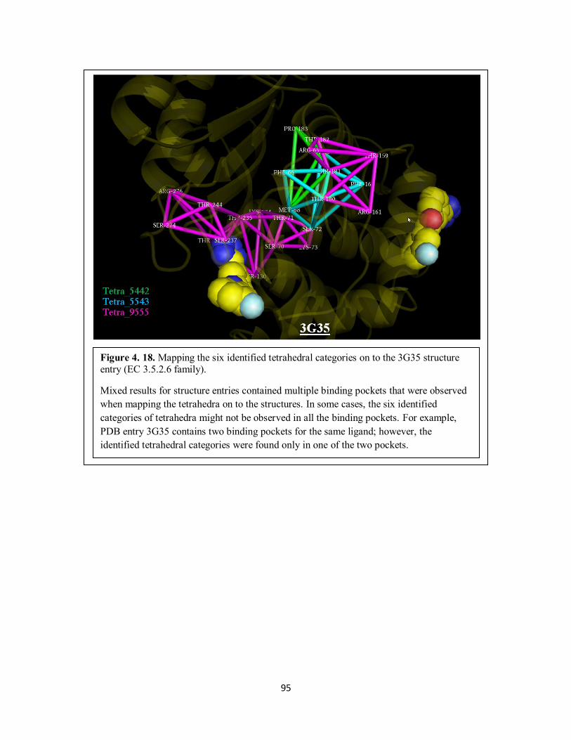
95

Figure 4. 18. Mapping the six identified tetrahedral categories on to the 3G35 structure entry (EC 3.5.2.6 family).

Mixed results for structure entries contained multiple binding pockets that were observed

when mapping the tetrahedra on to the structures. In some cases, the six identified

categories of tetrahedra might not be observed in all the binding pockets. For example,

PDB entry 3G35 contains two binding pockets for the same ligand; however, the

identified tetrahedral categories were found only in one of the two pockets.

96

4.7.4 Methyltransferases (EC 2.1.1)


obtained after applying the classification method described in Chapter 2 to separate the EC 2.1.1

from the enzyme diversity set. EC 2.1.1 contains enzymes with more generalized function as

hinted by the three-digit Enzyme Classification number and can be further classified into 195

subfamilies. As illustrated in Figure 4.19, the most significant model (with the highest z-score)

was built with the top

500 ranked features.

Although the model

was capable to

perfectly separate the

structure entries

associated with EC

2.1.1 from the enzyme

diversity set (both

sensitivity and

specificity equal to

one), it was not

feasible to analyze or

interpret the model due

to the large number of

features incorporated.

Figure 4. 19. Identifying the most significant model through z-

score for the EC 2.1.1 dataset.

This semi-log plot indicates the z-score associated with the top

500 features is the highest. The y-axis on the left (Percentage) is for sensitivity and specificity while the y-axis on the right is for z-

score.

97

4.7.5 Protein-Tyrosine Kinases (EC 2.7.10)



from the enzyme diversity set. EC 2.7.10 contains enzymes with more generalized function and

can be further classified into two additional subfamilies. As illustrated in Figure 4.20, both

models built with top 50 and top 100 ranked features achieved similar values in z-scores, which

are 7.09 and 7.06 respectively. Since the z-scores of these two models were above 7.0, we used

both sensitivity and specificity to guide the final selection of features. Based on the classification

performance (both

sensitivity and

specificity equal to

1.0), we selected the

top 100 ranked

features as the

important features

associated with

protein-tyrosine

kinases. Similarly to

the results for EC

2.1.1, it was not

feasible to analyze or

interpret the model

due to the large

number of features

incorporated.

Figure 4. 20. Identifying the most significant model through z-

score for the EC 2.7.10 dataset.

This semi-log plot indicates that the z-scores associated with the

top 50 and top 100 features are both similar in values. A model

built with top 100 features is selected for the performance in

sensitivity and specificity. The y-axis on the left (Percentage) is for sensitivity and specificity while the y-axis on the right is for z-

score.

98

4.7.6 Protein-Serine/Threonine Kinase (EC 2.7.11)



from the enzyme diversity set. EC 2.7.11 contains enzymes with more generalized function and

can be further classified into 31 subfamilies. As illustrated in Figure 4.21, the model built with

the top 1,000

ranked features

achieved the highest

z-score, sensitivity

(1.0), and

specificity (1.0). As

noted in other

results obtained

from enzymes with

more generalized

function, it was not

feasible to analyze

or interpret the

model due to the

large number of

features incorporated.

Figure 4. 21. Identifying the most significant model through z-scores for the EC 2.7.11 dataset.

This semi-log plot indicates the z-score associated with the top 1000 features is the highest. The y-axis on the left (Percentage) is for

sensitivity and specificity while the y-axis on the right is for z-

score.

99

4.8 Evaluating the Stability of the Delaunay Simplices

The definition of the Delaunay tessellation depends on the precise coordinate values

given to its points. In the scenario that point coordinates are known only imprecisely, the stability

and robustness of the resulting Delaunay simplices under changes to the input coordinates could

be questioned 14

. The results in enzyme families EC 1.15.1.1 and EC 3.5.2.6, where the Delaunay

simplices captured only one binding pocket of the two available, might be explained by the

imprecision of the input coordinates. In PDB entry, 3G35, there are two binding pockets for the

same ligand but the amino acid compositions for these two sites are completely different.

However, in the case of PDB entry, 1TO4, there are two identical binding pockets within the

structure, and the tetrahedral categories identified as significant to the protein function only

appeared in one of the two binding pockets.

To evaluate the stability and robustness of the Delaunay simplices, a Gaussian sphere

with a radius of approximately 0.5 Å was applied to each of the original Cα atom coordinates in

PDB entry, 1TO4, to permit the shifting of the points. The shifting of each Cα atom is

independent of one another, and 30 structures were generated with the new Cα coordinates.

Delaunay tessellation was then applied to these 30 modified structures, and tetrahedra with edges

longer than 12 Å were removed. Within each of the 30 tessellation outcomes, a search for the four

tetrahedral categories, i.e., 6600, 9995, 9997, and 9999, was performed. Figure 4.22 shows all the

tetrahedra associated with the four tetrahedral types that are found in the search result.

The three tetrahedra associated with category 6600 that were found in the original

structure also appeared in all the 30 modified structures. These tetrahedra were formed by the

amino acids Gly (9), Gly (55), Cys (56), Ala (144), and Cys (145). While the tetrahedron formed

by Gly (9), Gly(55), Cys (56), and Cys (145) was found in only one of the two chains, the

tetrahedron formed by Gly (9), Cys (56), Ala (144), and Cys (145) appeared in both chains.

100

For tetrahedral categories 9997, new tetrahedra were found in addition to the one

tetrahedron appearing in the original structure. The tetrahedron formed by amino acids His (62),

Asn (64), His (70), and His (79) that appeared in the original structure was also found on the

modified structures in 21out of 30 instances. The same four amino acids on the other chain also

formed a tetrahedron in 9 out of 30 instances of modified structures. Additionally, the

tetrahedron formed by Lys (38), Lys (41), His (42), and Asn (121) that did not appear in the

original structure was found in four out of the 30 instances.

The outcome from this evaluation indicated that the Delaunay simplices calculated solely

from the original X-ray crystal structures did not fully capture the comprehensive local

neighborhood relationship of the amino acids within a protein structure. By treating the atom

Figure 4. 22. Mapping the four categories of tetrahedron found in the modified structures onto the original 1TO4 PDB structure.

The tetrahedra that appeared in the original and modified structures are shown in stick and

line, respectively.

101

coordinates of a protein crystal structure as flexible points rather than fixed ones, the resulting

Delaunay simplices, which were obtained from a set of thirty structures with perturbed atom

coordinates, could capture a more comprehensive local neighborhood relationship of the amino

acids within the protein structure. Since our protocol for studying the protein structure-function

relationship was designed to utilize the atom coordinates as fixed points, this finding raised

concerns regarding the performance of our model in protein function prediction.

There are two possible methods to predict a protein function based on this developed

QSAR-like strategy: direct and indirect. The direction prediction, which is a straightforward

utilization of a model, would be most likely to suffer from a higher type II error (false negative)

caused by a set of simplices that did not fully capture the local packing order of amino acids in

protein structures. The same cause for a higher type II error would also likely affect indirect

prediction but with less impact, because an additional search for common simplices with similar

geometric properties was performed in the tetrahedral categories identified by the model. The

presence of these resulting common simplices would then be used to predict the function of other

protein structures that are not part of the training set. However, grouping simplices based on

similar geometric properties required additional analysis to critically assess the appropriate

binning of each geometric property, which was not part of the scope of this research; thus,

indirect prediction was not implemented in this research.

102

4.9 Comparison with PROSITE

PROSITE is a protein database consisting of manually curated amino acid profiles and

patterns that describe protein domains, families and functional sites. Applications of these profiles

and patterns include both identifying possible functions for newly discovered proteins and

analyzing known proteins for previously undetermined activities. These patterns were utilized in

this comparison study.

To compare the performance between our method and PROSITE, we used ScanPROSITE

44, a web-based tool for detecting protein sequences that match PROSITE patterns and/or profiles.

Additionally, a separate test set containing both positive and negative classes was selected to

benchmark both methods. Standard criteria for evaluating the performance of information

retrieval systems, such as precision, recall (sensitivity), and true negative rate (specificity), were

calculated to compare the two methods. For PROSITE evaluation, a PDB entry was considered to

be a positive hit if its sequence matched at least one of the evaluated PROSITE profiles or

patterns. In total, nine PROSITE patterns were utilized in this benchmark study – four patterns for

E.C. 1.15.1.1 and five patterns for E.C. 3.5.2.6.

4.9.1 Test Set Selection Criteria for Both E.C. 1.15.1.1 and E.C. 3.5.2.6

For the positive class, a set of PDB entries from family members belonging to either

E.C. 1.15.1.1 or E.C. 3.5.2.6 was created, while the negative class contained PDB entries from an

enzyme diversity set, excluding E.C. 1.15.1.1 and E.C. 3.5.2.6. The test set for each enzyme set,

i.e., E.C. 1.15.11 and E.C. 3.5.2.6, was created by combing the corresponding positive class with

the negative class. The selection criteria for the positive and negative classes were similar to that

of the enzyme class of interest and enzyme diversity set, respectively. This benchmark study

excluded E.C. 3.2.1.4 because none of the PROSITE patterns was specific for this particular

enzyme family.

103

Several criteria were used during the PDB entry selection to ensure the quality and size of

the test set. First, the X-ray resolution for the positive class of the test set was relaxed to 2.00 Å to

include a greater number of crystal structures. Structure entries previously included in our

modeling procedure were removed

from the test sets to allow for fair

comparison. Similarly, all entries

selected were released within the past

three years, i.e., between 01/01/2008

and 12/31/2011, to ensure that the

resulting structure entries were not

used in generating the PROSITE

signatures applied to this study, which

were last updated in 2006. The

resulting test sets, based on these

selection criteria, contained 421

structure entries for the negative class,

15 structure entries for E.C. 1.15.1.1

and 22 for E.C. 3.5.2.6. The PDB

entries for the two positive classes are

listed in Table 4.10.

4.9.2 Comparison Results

Both methods were able to retrieve the positive class for both E.C. 1.15.1.1 and E.C.

3.5.2.6 comparably well. For E.C. 1.15.1.1, our method achieved a recall (sensitivity) value of

0.87 by retrieving thirteen out of the fifteen PDB entries associated with the positive class while

ScanPROSITE was able to retrieve one addition entry and achieved a recall value of 0.93.

PDB

Entries

E.C.

Numbers

PDB

Entries

E.C.

Numbers

2JLP 1.15.1.1 2V1Z 3.5.2.6

2RCV 1.15.1.1 2WHG 3.5.2.6

2WYT 1.15.1.1 2WK0 3.5.2.6

3AK2 1.15.1.1 2X02 3.5.2.6

3DC5 1.15.1.1 2ZD8 3.5.2.6

3G4Z 1.15.1.1 2ZQ7 3.5.2.6

3H1S 1.15.1.1 3E2L 3.5.2.6

3JS4 1.15.1.1 3FKW 3.5.2.6

3K9S 1.15.1.1 3G4P 3.5.2.6

3KBE 1.15.1.1 3HBR 3.5.2.6

3KKY 1.15.1.1 3I11 3.5.2.6

3L9Y 1.15.1.1 3IOF 3.5.2.6

3LIO 1.15.1.1 3ISG 3.5.2.6

3LSU 1.15.1.1 3L6N 3.5.2.6

3PU7 1.15.1.1 3LEZ 3.5.2.6

3M8T 3.5.2.6

3MZF 3.5.2.6

3NY4 3.5.2.6

3P09 3.5.2.6

3Q6V 3.5.2.6

3Q6X 3.5.2.6

3S1Y 3.5.2.6

Table 4. 10. The list of PDB entries selected for

the two positive classes.

104

However, when comparing the two lists of retrieval entries, only twelve entries were correctly

identified by both methods. ScanPROSITE failed to identify 3G4Z, while our model missed 3JS4

and 3KBE. The failure to identify 3G4Z by PROSITE was likely due to the lack of manually

curated patterns for the nickel-binding SOD, which belonged to E.C. 1.15.1.1. A similar outcome

was also observed in the test set for E.C. 3.5.2.6. Both methods were able to retrieve twelve out of

the twenty-two PDB entries from the positive class, yielding a recall value of 0.55. Comparison

of each of the twelve entries identified indicated only four common entries between the two

methods. Used together, 100% of the positive class was correctly identified for E.C. 1.15.1.1, and

91% of the positive class was identified for E.C. 3.5.2.6, suggesting that the two protocols are

potentially complementary. Figure 4.23 shows the benchmarking results.

Figure 4. 23. Benchmarking results.

Both methods performed similarly in sensitivity and specificity. When used together,

we observe an increase in sensitivity for both E.C. 1.15.1.1 and E.C. 3.5.2.6, suggesting

that the two protocols are potentially complementary.

105

However, ScanPROSITE identified no false positives for either test set, while our method

incorrectly labeled 33 negatives (0.93 in true negative rate or specificity) and 50 (0.87 in true

negative rate or specificity) in the E.C. 1.15.1.1 and E.C. 3.5.2.6 datasets, respectively. Due to the

number of false positives (or type I error) in our model, the precision of our models for predicting

the test sets for E.C. 1.15.1.1 and E.C. 3.5.2.6 was 0.28 and 0.19, respectively.

To improve the number of true positives and false positives predicted by our model, two

possible enhancements could be made to our protein descriptors that would enable DWD-VS to

identify a more specific set of Delaunay simplices that contributed to a given enzyme function.

Our protein descriptors, which utilized Delaunay simplices to characterize protein structures,

could be enhanced by considering protein structures obtained from experimental X-ray

crystallography as flexible entities rather than rigid ones. By calculating the protein descriptors

from a set of movable points instead of fixed ones, the Delaunay simplices could then be able to

capture a more comprehensive local neighborhood relationship between Cα atoms, as was

observed in our Delaunay simplices stability evaluation (Section 4.7).

Additionally, we could further distinguish Delaunay simplices with additional geometric

characteristics, such as chirality and volume. Especially the chirality of a Delaunay simplex,

which could be defined by the four amino acid vertices and the Cahn-Ingold-Prelog priority rules,

would provide the relative spatial orientation of the four amino acids to distinguish between

Delaunay simplices with the same composition.

4.10 Conclusion

The goal for implementing the protein descriptors was to study the structure-function

relationship of proteins. By combining variable selection DWD with the novel protein descriptors,

our intention was to identify important amino acids that are common in proteins with similar

functions. The results of our study indicated that our QSAR-like strategy helped to identify

groups of amino acid residues located near the corresponding binding ligand, which indicated that

106

the identified amino acids could be part of the binding pocket. Additionally, categorized

Delaunay simplices and their geometric properties were found to encode valuable structural

information and enabled DWD-VS to identify a specific set of Delaunay simplices that attributed

to a given enzyme function, especially when enzyme function was more specific, such as

observed in the studies of EC 1.15.1.1, EC 3.2.1.4, and EC 3.5.2.6. Mapping identified Delaunay

simplices onto their corresponding protein structures provided insights and led to generation of

hypotheses regarding the important binding residues.

The results of the comparison study for E.C. 1.15.1.1 and E.C. 3.5.2.6 against

ScanPROSITE indicated that when combining the protein descriptors with variable selection

DWD could provide a potentially complementary method to PROSITE, which utilizes expert

knowledge to annotate protein functions. Currently, this automated strategy is based on objective

structural data and proof of the concept for use of a QSAR-like analysis for protein function

annotation. Additional enhancements to the protein descriptors, such as flexible structure

sampling and geometric categorization of Delaunay simplices, would likely improve the precision

and recall for this QSAR-like strategy.

For applicability in future studies of protein families and for predicting structures with

unknown functions, the prediction procedure will also have to improve. One possible

improvement could result from the coupling of direct and indirect prediction using our method.

Specifically, direct prediction involves using a model built for a specific protein family, while

indirect prediction (discussed in Section 4.7) refers to a similarity search for tetrahedra within the

training set that display similar geometric characteristics, i.e., the use similar tetrahedra to imply

similar function.

Overall, our automated method showed comparable sensitivity to that of ScanPROSITE,

which showed considerable improvement and complementarity when the two methods were

combined. However, our method suffers from poor specificity, a problem that could likely be

resolved with the addition of the geometric descriptors mentioned above and by the use of both

107

direct and indirect prediction. Despite this drawback, the complementary results suggest that our

automated method is able to correctly identify functionally similar proteins that PROSITE

patterns, which were curated using expert knowledge, completely miss. The nature of these

missed proteins suggests that our method is better at identifying protein functional homologs with

a more distant similarity. Thus, our method could prove useful for more difficult protein

annotation, especially with further improvement and refinement of the protein descriptors.

Chapter 5

Summary

The increasing availability of biological and chemical data has led to a critical need for

cheminformatics and bioinformatics tools to analyze the data. One of the major challenges

involved in this data analysis is HDLSS. To overcome the statistical difficulties inherent in

HDLSS data, DWD was improved by adding variable selection. In a simulation using imbalanced,

HDLSS data, DWD with variable selection (DWD-VS) significantly improved model prediction

performance compared to SVM and DWD without variable selection. Analysis of models

indicated that DWD-VS consistently achieved high-prediction accuracy by removing greater than

99.9% of the noise while retaining up to 70% of the signal through informative descriptors. These

simulation results suggested that DWD-VS could be used to obtain a better understanding of the

underlying biological activities; thus, DWD-VS could provide faster and more cost-effective

models by identifying predictor variables to achieve high prediction accuracy. Similar results

were also observed in QSAR studies; however, the differences between SVM, DWD, and DWD-

VS were all too small to claim one method is much better than the others based solely on the

prediction accuracy.

While the strategies used to build predictive models are important for identifying the

structure-activity relationship of biomolecules, it is also essential to employ descriptors that

encode molecular characteristics associated with a target property. The 3D chiral atom-pair

descriptors were developed to evaluate the effect that the degree of chirality contributes to various

target properties. For the selected stereochemistry-dependent datasets, the 3D chiral atom-pair

descriptors showed better classification performance than 3D non-chiral atom-pair descriptors

(without chiral atom types), and as expected, both sets of 3D atom-pair descriptors performed

109

better than 2D Dragon descriptors. Not unexpectedly, for datasets with minimal chirality

information, classification performance of developed chirality-sensitive descriptors is similar to

the performance with either 2D Dragon or 3D chirality-insensitive atom-pair descriptors.

The QSAR studies of the stereochemistry dependent datasets also suggested that the

variable selection procedure implemented in the DWD-VS was likely to miss groups of

descriptors that contributed to biological activity but were highly correlated to one another. For

two datasets where the effect of stereochemistry on biological activities was not apparent, lower

prediction accuracy was observed in the DWD-VS models obtained from the combined

descriptors (2D Dragon + either 3D chiral atom-pair or 3D non-chiral atom-pair descriptors) than

DWD-VS models obtained from each of the 3D atom-pair descriptors alone. By using a simple

merge to combine different descriptor matrices, more instances of highly correlated descriptors

are likely to occur, especially if 3D atom-pair descriptors encode redundant information as the 2D

Dragon descriptors. These highly correlated descriptors affect the weighting assigned by DWD

internal algorithms, causing the descriptors that should be selected to be dropped instead. To

improve the performance of the variable selection DWD, correlation between descriptors will

have to be considered as part of the variable selection procedure.

To study the structure-function relationship of proteins, combining novel protein

descriptors with DWD-VS provided a potential complement to ScanPROSITE, which utilized

expert knowledge to annotate protein function. This QSAR-like strategy helped to identify groups

of amino acid residues that were a part of the binding pocket, as observed in the studies of EC

1.15.1.1, EC 3.2.1.4, and EC 3.5.2.6. Mapping identified tetrahedra onto the corresponding

protein structures provided insights and hypotheses on the important binding residues; however, it

also indicated two drawbacks of the protein descriptors. First, Delaunay simplices in protein

structures are sensitive to the imprecision of the input coordinates -- some examples capture one

binding pocket when there are multiple binding pockets available. Second, if multiple tetrahedra

from the same category are identified as significant, the current implementation of tetrahedral

110

categories does not allow users to further narrow down these tetrahedra to a smaller set that is

critical to binding. To address the first shortcoming, one solution is to apply a Gaussian sphere

around each coordinate to sample other likely locations of the atoms and then generate a

descriptor matrix that summarizes all the resulting Delaunay simplices and their associated

geometric properties. This solution is likely to address only the scenario where multiple binding

pockets within a protein structure have the same amino acid composition, e.g. PDB entry 1TO4.

In the case of multiple binding pockets that are different in amino acid composition, e.g. PDB

entry 3G35, the binding pocket that was not identified in our result may not be the primary site

since the original literature only focused on the binding pocket identified in this research. As for

the second shortcoming, a possible solution would be to further categorize the tetrahedron based

on values of geometric properties.

In summary, the outcomes of this research provide cheminformatics and bioinformatics

tools for modeling and analyzing the structure-activity relationship within biomolecular data

through novel molecular descriptors and a variable selection based statistical machine learning

method. Specifically, the technologies set forth in this dissertation address the HDLSS

imbalanced categorical characteristics present in many biomolecular datasets. The data evaluated

in this research were embedded in dimension that ranged from 2 to 42 times the sample size, and

multiple imbalanced categorical datasets were evaluated, including datasets with the positive

class contributing less than 5% of the total data. Our results indicated that DWD-VS gave models

with high external prediction power and the estimated intrinsic dimension that is usually lower

than the sample size and contained predictive descriptors that characterize the target biological

property. We also showed that the developed chirality-sensitive descriptors increased the

predictive power of QSAR models obtained for stereochemistry dependent datasets. In addition

we demonstrated that our method is better at identifying protein functional homologs with a more

distant similarity and could prove useful for more difficult protein annotation, especially with

further improvement and refinement of the protein descriptors. Overall, these developed

111

descriptors and DWD-VS provide not only tools for modeling and analyzing the structure-activity

relationship of biomolecular data but also direction for future advancements in chemical

compound and protein classification.

112

Reference List

1. Enzyme Nomenclature 1992: Recommendations of the NCIUBMB on the Nomenclature

and Classification of Enzymes; Academic Press Inc: San Diego, 1992; pp 1-862.

2. Global Chiral Technology Markets. 3-1-2001. Frost & Sullivan.

Ref Type: Report

3. Dragon for Windows (Software for Molecular Descriptor Calculations). [5.5]. 2009. Milan (Italy), TALETE S.R.L.

Ref Type: Computer Program

4. Adibi, S. A. The oligopeptide transporter (Pept-1) in human intestine: Biology and

function. Gastroenterology 1997, 113, 332-340.

5. Adibi, S. A. Regulation of expression of the intestinal oligopeptide transporter (Pept-1) in

health and disease. American Journal of Physiology-Gastrointestinal and Liver

Physiology 2003, 285, G779-G788.

6. Agranat, I.; Caner, H.; and Caldwell, A. Putting chirality to work: The strategy of chiral

switches. Nature Reviews Drug Discovery 2002, 1, 753-768.

7. Aires-de-Sousa, J.; Gasteiger, J.; Gutman, I.; and Vidovic, D. I. Chirality codes and molecular structure. Journal of Chemical Information and Computer Sciences

2004, 44, 831-836.

8. Altschul, S. F.; Gish, W.; Miller, W.; Myers, E. W.; and Lipman, D. J. Basic Local

Alignment Search Tool. Journal of Molecular Biology 1990, 215, 403-410.

9. Altschul, S. F.; Madden, T. L.; Schaffer, A. A.; Zhang, J. H.; Zhang, Z.; Miller, W.; and

Lipman, D. J. Gapped BLAST and PSI-BLAST: a new generation of protein

database search programs. Nucleic Acids Research 1997, 25, 3389-3402.

10. Anfinsen, C. B. Principles That Govern Folding of Protein Chains. Science 1973, 181,

223-230.

11. Avnir,D.; Hel-Or,H.Z.; and Mezey,P.G. Symmetry and Chirality: Continuous Measures. In The Encyclopedia of Computational Chemistry. Schleyer, P. v. R., Allinger, N.

L., Clark, T., Gasteiger, J., Kollman, P. A. H. F., and Schreiner, P. R. Eds.; John

Wiley & Sons Ltd: Chichester, 1998; pp 2890-2901.

12. Bagley, S. C. and Altman, R. B. Characterizing the Microenvironment Surrounding Protein Sites. Protein Science 1995, 4, 622-635.

13. Bailey, P. D.; Boyd, C. A. R.; Bronk, J. R.; Collier, I. D.; Meredith, D.; Morgan, K. M.;

and Temple, C. S. How to make drugs orally active: A substrate template for peptide transporter PepT1. Angewandte Chemie-International Edition 2000, 39,

506-+.

113

14. Bandyopadhyay, D. and Snoeyink, J. Almost-Delaunay simplices: Robust neighbor

relations for imprecise 3D points using CGAL. Computational Geometry-Theory and Applications 2007, 38, 4-15.

15. Bartlett, G. J.; Porter, C. T.; Borkakoti, N.; and Thornton, J. M. Analysis of catalytic

residues in enzyme active sites. Journal of Molecular Biology 2002, 324, 105-

121.

16. Baskin, I.; Radchenko, E. V.; Palyulin, V. A.; Zefirov, N. S.; Proschak, E.; Tanrikulu, Y.;

Schneider, G.; Tropsha, A.; Horvath, D.; Zheng, W.; Johnson, S. R.; Filimonov,

D.; Poroikov, V.; Laggner, C.; Wolber, G.; Kirchmair, J.; Schuster, D.; Langer, T.; Peltason, L.; Bajorath, J.; Tetko, I. V.; and Opr, T. I. Chemoinformatics

Approaches to Virtual Screening; Royal Society of Chemistry: 2008; pp 1-355.

17. Baylin, S. and Bestor, T. H. Altered methylation patterns in cancer cell genomes: Cause or consequence? Cancer Cell 2002, 1, 299-305.

18. Baylin, S. B. and Herman, J. G. DNA hypermethylation in tumorigenesis - epigenetics

joins genetics. Trends in Genetics 2000, 16, 168-174.

19. Berman, H. M.; Westbrook, J.; Feng, Z.; Gilliland, G.; Bhat, T. N.; Weissig, H.; Shindyalov, I. N.; and Bourne, P. E. The Protein Data Bank. Nucleic Acids

Research 2000, 28, 235-242.

20. Biegel, A.; Gebauer, S.; Hartrodt, B.; Brandsch, M.; Neubert, K.; and Thondorf, I. Three-dimensional quantitative structure-activity relationship analyses of beta-lactam

antibiotics and tripeptides as substrates of the mammalian H+/peptide

cotransporter PEPT1. Journal of Medicinal Chemistry 2005, 48, 4410-4419.

21. Binkowski, T. A.; Adamian, L.; and Liang, J. pvSoar: Pocket and void surfaces of amino

acid residues. Biophysical Journal 2004, 86, 490A.

22. Binkowski, T. A.; Freeman, P.; and Liang, J. pvSOAR: detecting similar surface patterns

of pocket and void surfaces of amino acid residues on proteins. Nucleic Acids Research 2004, 32, W555-W558.

23. Binkowski, T. A. and Joachimiak, A. Protein Functional Surfaces: Global Shape

Matching and Local Spatial Alignments of Ligand Binding Sites. Bmc Structural Biology 2008, 8.

24. Brandsch, M. Transport of drugs by proton-coupled peptide transporters: pearls and

pitfalls. Expert Opinion on Drug Metabolism & Toxicology 2009, 5, 887-905.

25. Brandsch, M.; Knutter, I.; and Leibach, F. H. The intestinal H+/peptide symporter PEPT1: structure-affinity relationships. European Journal of Pharmaceutical Sciences

2004, 21, 53-60.

26. Bretschneider, B.; Brandsch, M.; and Neubert, R. Intestinal transport of beta-lactam antibiotics: Analysis of the affinity at the H+/peptide symporter (PEPT1), the

uptake into Caco-2 cell monolayers and the transepithelial flux. Pharmaceutical

Research 1999, 16, 55-61.

114

27. Bru, C.; Courcelle, E.; Carrre, S.; Beausse, Y.; Dalmar, S.; and Kahn, D. The ProDom

database of protein domain families: more emphasis on 3D. Nucleic Acids Research 2005, 33, D212-D215.

28. Buda, A. B. and Mislow, K. On Geometric Measures of Chirality. Theochem-Journal of

Molecular Structure 1991, 78, 1-12.

29. Caldwell, J. Through the looking glass in chiral drug cevelopment. Modern Drug Discovery 1999, 2.

30. Caner, H.; Groner, E.; Levy, L.; and Agranat, I. Trends in the development of chiral

drugs. Drug Discovery Today 2004, 9, 105-110.

31. Capra, M.; Nuciforo, P. G.; Confalonieri, S.; Quarto, M.; Bianchi, M.; Nebuloni, M.;

Boldorini, R.; Pallotti, F.; Viale, G.; Gishizky, M. L.; Draetta, G. F.; and Di Fiore,

P. P. Frequent alterations in the expression of serine/threonine kinases in human cancers. Cancer Research 2006, 66, 8147-8154.

32. Carhart, R. E.; Smith, D. H.; and Venkataraghavan, R. Atom Pairs As Molecular-Features

in Structure Activity Studies - Definition and Applications. Journal of Chemical

Information and Computer Sciences 1985, 25, 64-73.

33. Carter, C. W.; LeFebvre, B. C.; Cammer, S. A.; Tropsha, A.; and Edgell, M. H. Four-

body potentials reveal protein-specific correlations to stability changes caused by

hydrophobic core mutations. Journal of Molecular Biology 2001, 311, 625-638.

34. Castillo-Garit, J. A.; Marrero-Ponce, Y.; Torrens, F.; and Rotondo, R. Atom-based

stochastic and non-stochastic 3D-chiral bilinear indices and their applications to

central chirality codification. Journal of Molecular Graphics & Modelling 2007, 26, 32-47.

35. Chen, L. H.; Kenyon, G. L.; Curtin, F.; Harayama, S.; Bembenek, M. E.; Hajipour, G.;

and Whitman, C. P. 4-Oxalocrotonate Tautomerase, An Enzyme Composed of 62

Amino-Acid-Residues Per Monomer. Journal of Biological Chemistry 1992, 267, 17716-17721.

36. Chen, Y. and Shoichet, B. K. Molecular docking and ligand specificity in fragment-based

inhibitor discovery. Nat Chem Biol. 2009, 5, 358-364.

37. Chothia, C. and Lesk, A. M. The Relation Between the Divergence of Sequence and

Structure in Proteins. Embo Journal 1986, 5, 823-826.

38. Clarke, S. The Role of Protein Methylation Reactions in Signal Transduction and the

Repair of Damaged Proteins. Abstracts of Papers of the American Chemical Society 1991, 201, 83-MEDI.

39. Clarke, S. Aging as war between chemical and biochemical processes: Protein

methylation and the recognition of age-damaged proteins for repair. Ageing Research Reviews 2003, 2, 263-285.

40. Collaborative Drug Discovery. CCD Public. 2004.

115


41. Conwit, R. A. Preventing familial ALS: A clinical trial may be feasible but is an efficacy trial warranted? Journal of the Neurological Sciences 2006, 251, 1-2.

42. Crippen, G. M. Chirality Descriptors in QSAR. Current Computer-Aided Drug Design

2008, 4, 259-264.

43. Das, P. M. and Singal, R. DNA methylation and cancer. Journal of Clinical Oncology 2004, 22, 4632-4642.

44. de Castro, E.; Sigrist, C. J. A.; Gattiker, A.; Bulliard, V.; Langendijk-Genevaux, P. S.;

Gasteiger, E.; Bairoch, A.; and Hulo, N. ScanProsite: detection of PROSITE signature matches and ProRule-associated functional and structural residues in

proteins. Nucleic Acids Research 2006, 34, W362-W365.

45. Dervarics, M.; Otvos, F.; and Martinek, T. A. Development of a chirality-sensitive flexibility descriptor for 3+3D-QSAR. Journal of Chemical Information and

Modeling 2006, 46, 1431-1438.

46. Devlin, T. M. Textbook of Biochemistry with Clinical Correlations; Wiley-Liss: 2006; pp

1-1896.

47. Ding Z. Diversified Ensemble Classifiers for Highly Imbalanced Data Learning and their

Application in Bioinformatics. 1-116. 5-7-2011. Georgia State University.

Ref Type: Thesis/Dissertation

48. Doring, F.; Walter, J.; Will, J.; Focking, M.; Boll, M.; Amasheh, S.; Clauss, W.; and

Daniel, H. Delta-aminolevulinic acid transport by intestinal and renal peptide

transporters and its physiological and clinical implications. Journal of Clinical Investigation 1998, 101, 2761-2767.

49. Duca, J. S. and Hopfinger, A. J. Estimation of molecular similarity based on 4D-QSAR

analysis: Formalism and validation. Journal of Chemical Information and

Computer Sciences 2001, 41, 1367-1387.

50. Duda, R. O.; Hart, P. E.; and Stork, D. G. Pattern Classification; Wiley-Interscience:

2000; pp 1-654.

51. Dunaway-Mariano, D. Enzyme Function Discovery. Structure 2008, 16, 1599-1600.

52. Dundas, J.; Ouyang, Z.; Tseng, J.; Binkowski, A.; Turpaz, Y.; and Liang, J. CASTp:

computed atlas of surface topography of proteins with structural and

topographical mapping of functionally annotated residues. Nucleic Acids

Research 2006, 34, W116-W118.

53. Eichelbaum,M. and Gross A.S. Stereochemical aspects of drug action and disposition.

Testa, B. and Meyer, U. A. Eds.; Elsevier: 1996; pp 1-64.

116

54. Finn, R. D.; Tate, J.; Mistry, J.; Coggill, P. C.; Sammut, S. J.; Hotz, H. R.; Ceric, G.;

Forslund, K.; Eddy, S. R.; Sonnhammer, E. L. L.; and Bateman, A. The Pfam protein families database. Nucleic Acids Research 2008, 36, D281-D288.

55. Food and Drug Administration. FDA's policy statement for the development of new

stereoisomeric drugs. 5-1-1992.

Ref Type: Bill/Resolution

56. Ganapathy, M. E.; Brandsch, M.; Prasad, P. D.; Ganapathy, V.; and Leibach, F. H.

Differential Recognition of Beta-Lactam Antibiotics by Intestinal and Renal

Peptide Transporters, Pept-1 and Pept-2. Journal of Biological Chemistry 1995, 270, 25672-25677.

57. Ganapathy, M. E.; Huang, W.; Wang, H.; Ganapathy, V.; and Leibach, F. H.

Valacycloviv: A substrate for the intestinal and renal peptide transporters PEPT1 and PEPT2. Biochemical and Biophysical Research Communications 1998, 246,

470-475.

58. Glaser, F.; Morris, R. J.; Najmanovich, R. J.; Laskowski, R. A.; and Thornton, J. M. A

method for localizing ligand binding pockets in protein structures. Proteins-Structure Function and Bioinformatics 2006, 62, 479-488.

59. Glaser, F.; Rosenberg, Y.; Kessel, A.; Pupko, T.; and Ben Tal, N. The ConSurf-HSSP

database: The mapping of evolutionary conservation among homologs onto PDB structures. Proteins-Structure Function and Bioinformatics 2005, 58, 610-617.

60. Golbraikh, A.; Bonchev, D.; and Tropsha, A. Novel chirality descriptors derived from

molecular topology. Journal of Chemical Information and Computer Sciences 2001, 41, 147-158.

61. Golbraikh, A.; Bonchev, D.; and Tropsha, A. Novel ZE-isomerism descriptors derived

from molecular topology and their application to QSAR analysis. Journal of

Chemical Information and Computer Sciences 2002, 42, 769-787.

62. Golbraikh, A. and Tropsha, A. QSAR Modeling using chirality descriptors derived from

molecular topology. Journal of Chemical Information and Computer Sciences

2003, 43, 144-154.

63. Guyon, I. and Elisseeff A. An Introduction to Variable and Feature Selection. Journal of

Machine Learning Research 2003, 3, 1157-1182.

64. Han, H. K. and Amidon, G. L. Targeted prodrug design to optimize drug delivery. Aaps

Pharmsci 2000, 2.

65. Holm, L. and Sander, C. Protein structure comparison by alignment of distance matrices.

Journal of Molecular Biology 1993, 233, 123-138.

66. Holten, K. B. and Onusko, E. M. Appropriate prescribing of oral beta-lactam antibiotics. American Family Physician 2000, 62, 611-620.

117

67. Huan, J.; Bandyopadhyay, D.; Wang, W.; Snoeyink, J.; Prins, J.; and Tropsha, A.

Comparing graph representations of protein structure for mining family-specific residue-based packing motifs. Journal of Computational Biology 2005, 12, 657-

671.

68. Hulo, N.; Bairoch, A.; Bulliard, V.; Cerutti, L.; Cuche, B. A.; de Castro, E.; Lachaize, C.;

Langendijk-Genevaux, P. S.; and Sigrist, C. J. A. The 20 years of PROSITE. Nucleic Acids Research 2008, 36, D245-D249.

69. Ivanisenko, V. A.; Pintus, S. S.; Grigorovich, D. A.; and Kolchanov, N. A. PDBSiteScan:

a program for searching for active, binding and posttranslational modification sites in the 3D structures of proteins. Nucleic Acids Research 2004, 32, W549-

W554.

70. Jacoby, G. A. AmpC beta-Lactamases. Clinical Microbiology Reviews 2009, 22, 161-+.

71. Jaeger, K. E. and Eggert, T. Enantioselective biocatalysis optimized by directed evolution.

Current Opinion in Biotechnology 2004, 15, 305-313.

72. Julian-Ortiz, J. V.; Alapont, C. D.; Rios-Santamarina, I.; Garcia-Domenech, R.; and

Galvez, J. Prediction of properties of chiral compounds by molecular topology. Journal of Molecular Graphics & Modelling 1998, 16, 14-18.

73. Kolodny, R.; Koehl, P.; and Levitt, M. Comprehensive evaluation of protein structure

alignment methods: Scoring by geometric measures. Journal of Molecular Biology 2005, 346, 1173-1188.

74. Kovatcheva, A.; Buchbauer, G.; Golbraikh, A.; and Wolschann, P. QSAR modeling of

alpha-campholenic derivatives with sandalwood odor. Journal of Chemical Information and Computer Sciences 2003, 43, 259-266.

75. Kovatcheva, A.; Golbraikh, A.; Oloff, S.; Feng, J.; Zheng, W.; and Tropsha, A. QSAR

modeling of datasets with enantioselective compounds using chirality sensitive

molecular descriptors. Sar and Qsar in Environmental Research 2005, 16, 93-102.

76. Kovatcheva, A.; Golbraikh, A.; Oloff, S.; Xiao, Y. D.; Zheng, W. F.; Wolschann, P.;

Buchbauer, G.; and Tropsha, A. Combinatorial QSAR of ambergris fragrance compounds. Journal of Chemical Information and Computer Sciences 2004, 44,

582-595.

77. Krause, D. S. and Van Etten, R. A. Tyrosine kinases as targets for cancer therapy. New

England Journal of Medicine 2005, 353, 172-187.

78. Krishnamoorthy, B. and Tropsha, A. Development of a four-body statistical pseudo-

potential to discriminate native from non-native protein conformations.

Bioinformatics 2003, 19, 1540-1548.

79. Krissinel, E. and Henrick, K. Secondary-structure matching (SSM), a new tool for fast

protein structure alignment in three dimensions. Acta Crystallographica Section

D-Biological Crystallography 2004, 60, 2256-2268.

118

80. Kuz'min, V. E.; Artemenko, A. G.; Polischuk, P. G.; Muratov, E. N.; Hromov, A. I.;

Liahovskiy, A. V.; Andronati, S. A.; and Makan, S. Y. Hierarchic system of QSAR models (1D-4D) on the base of simplex representation of molecular

structure. Journal of Molecular Modeling 2005, 11, 457-467.

81. Landau, M.; Mayrose, I.; Rosenberg, Y.; Glaser, F.; Martz, E.; Pupko, T.; and Ben Tal, N.

ConSurf 2005: the projection of evolutionary conservation scores of residues on protein structures. Nucleic Acids Research 2005, 33, W299-W302.

82. Laskowski, R. A. Surfnet - A Program for Visualizing Molecular-Surfaces, Cavities, and

Intermolecular Interactions. Journal of Molecular Graphics 1995, 13, 323-&.

83. Laskowski, R. A.; Luscombe, N. M.; Swindells, M. B.; and Thornton, J. M. Protein clefts

in molecular recognition and function. Protein Science 1996, 5, 2438-2452.

84. Laskowski, R. A.; Watson, J. D.; and Thornton, J. M. ProFunc: a server for predicting protein function from 3D structure. Nucleic Acids Research 2005, 33, W89-W93.

85. Letunic, I.; Copley, R. R.; Pils, B.; Pinkert, S.; Schultz, J.; and Bork, P. SMART 5:

domains in the context of genomes and networks. Nucleic Acids Research 2006,

34, D257-D260.

86. Li, T. P.; Fan, K.; Wang, J.; and Wang, W. Reduction of protein sequence complexity by

residue grouping. Protein Engineering 2003, 16, 323-330.

87. Lichtarge, O.; Bourne, H. R.; and Cohen, F. E. An evolutionary trace method defines binding surfaces common to protein families. Journal of Molecular Biology 1996,

257, 342-358.

88. Loewenstein, Y.; Raimondo, D.; Redfern, O. C.; Watson, J.; Frishman, D.; Linial, M.; Orengo, C.; Thornton, J.; and Tramontano, A. Protein function annotation by

homology-based inference. Genome Biology 2009, 10.

89. Madej, T.; Gibrat, J. F.; and Bryant, S. H. Threading A Database of Protein Cores.

Proteins-Structure Function and Genetics 1995, 23, 356-369.

90. Marchler-Bauer, A.; Anderson, J. B.; Cherukuri, P. F.; DeWweese-Scott, C.; Geer, L. Y.;

Gwadz, M.; He, S. Q.; Hurwitz, D. I.; Jackson, J. D.; Ke, Z. X.; Lanczycki, C. J.;

Liebert, C. A.; Liu, C. L.; Lu, F.; Marchler, G. H.; Mullokandov, M.; Shoemaker, B. A.; Simonyan, V.; Song, J. S.; Thiessen, P. A.; Yamashita, R. A.; Yin, J. J.;

Zhang, D. C.; and Bryant, S. H. CDD: a conserved domain database for protein

classification. Nucleic Acids Research 2005, 33, D192-D196.

91. Markov, V. M.; Potyomkin, V. A.; and Belik, A. V. Evaluating a degree of molecular symmetry and chirality. Journal of Structural Chemistry 2001, 42, 76-83.

92. Marron, J. S.; Todd, M. J.; and Ahn, J. Distance-weighted discrimination. Journal of the

American Statistical Association 2007, 102, 1267-1271.

119

93. Mezey, P. G. The proof of the metric properties of a fuzzy chirality measure of molecular

electron density clouds. Journal of Molecular Structure-Theochem 1998, 455, 183-190.

94. Moreau, G. Atomic chirality, a quantitative measure of the chirality of the environment of

an atom. Journal of Chemical Information and Computer Sciences 1997, 37, 929-

938.

95. Mulder, N. J.; Apweiler, R.; Attwood, T. K.; Bairoch, A.; Bateman, A.; Binns, D.; Bork,

P.; Buillard, V.; Cerutti, L.; Copley, R.; Courcelle, E.; Das, U.; Daugherty, L.;

Dibley, M.; Finn, R.; Fleischmann, W.; Gough, J.; Haft, D.; Hulo, N.; Hunter, S.; Kahn, D.; Kanapin, A.; Kejariwal, A.; Labarga, A.; Langendijk-Genevaux, P. S.;

Lonsdale, D.; Lopez, R.; Letunic, I.; Madera, M.; Maslen, J.; McAnulla, C.;

McDowall, J.; Mistry, J.; Mitchell, A.; Nikolskaya, A. N.; Orchard, S.; Orengo, C.; Petryszak, R.; Selengut, J. D.; Sigrist, C. J. A.; Thomas, P. D.; Valentin, F.;

Wilson, D.; Wu, C. H.; and Yeats, C. New developments in the InterPro database.

Nucleic Acids Research 2007, 35, D224-D228.

96. Nakanishi, T.; Tamai, I.; Takaki, A.; and Tsuji, A. Cancer cell-targeted drug delivery utilizing oligopeptide transport activity. International Journal of Cancer 2000,

88, 274-280.

97. National Center for Biotechnology Information. PubChem. 2004. Ref Type: Computer Program

98. Nirmalananthan, N. and Greensmith, L. Amyotrophic lateral sclerosis: recent advances

and future therapies. Current Opinion in Neurology 2005, 18, 712-719.

99. OpenEye. QUACPAC. [1.3.1]. 7-3-2008.


100. OpenEye. OMEGA. [2.4.2]. 2010.


101. Oprea, T. I.; Tropsha, A.; Faulon, J. L.; and Rintoul, M. D. Systems chemical biology.

Nature Chemical Biology 2007, 3, 447-450.

102. Pal, D. and Eisenberg, D. Inference of protein function from protein structure. Structure 2005, 13, 121-130.

103. Petsko, G. A. and Ringe D. Protein Structure and Function; New Science Press, Ltd:

London, UK, 2003; pp 1-195.

104. Ponce, Y. M.; Diz, H. G.; Zaldivar, V. R.; Torrens, F.; and Castro, E. A. 3D-chiral quadratic indices of the 6 molecular pseudograph's atom adjacency matrix' and

their application to central chirality codification: classification of ACE inhibitors

and prediction of sigma-receptor antagonist activities. Bioorganic & Medicinal Chemistry 2004, 12, 5331-5342.

120

105. Porter, C. T.; Bartlett, G. J.; and Thornton, J. M. The Catalytic Site Atlas: a resource of

catalytic sites and residues identified in enzymes using structural data. Nucleic Acids Research 2004, 32, D129-D133.

106. Portugaly, E.; Linial, N.; and Linial, M. EVEREST: a collection of evolutionary

conserved protein domains. Nucleic Acids Research 2007, 35, D241-D246.

107. Qiao, X. Y. and Liu, Y. F. Adaptive Weighted Learning for Unbalanced Multicategory Classification. Biometrics 2009, 65, 159-168.

108. Qiao, X. Y.; Zhang, H. H.; Liu, Y. F.; Todd, M. J.; and Marron, J. S. Weighted Distance

Weighted Discrimination and Its Asymptotic Properties. Journal of the American Statistical Association 2010, 105, 401-414.

109. Radunovic, A. and Leigh, P. N. ALSODatabase: Database of SOD1 (and other) gene

mutations in ALS on the Internet. Amyotrophic Lateral Sclerosis and Other Motor Neuron Disorders 1999, 1, 45-49.

110. Rose, P. W.; Beran, B.; Bi, C. X.; Bluhm, W. F.; Dimitropoulos, D.; Goodsell, D. S.;

Prlic, A.; Quesada, M.; Quinn, G. B.; Westbrook, J. D.; Young, J.; Yukich, B.;

Zardecki, C.; Berman, H. M.; and Bourne, P. E. The RCSB Protein Data Bank: redesigned web site and web services. Nucleic Acids Research 2011, 39, D392-

D401.

111. Roskoski, R. The ErbB/HER receptor protein-tyrosine kinases and cancer. Biochemical and Biophysical Research Communications 2004, 319, 1-11.

112. Roth, B. L. and Driscoll, B. S. PDSP. 2011.


113. Rouhi, A. M. Chiral roundup - As pharmaceutical companies face bleak prospects, their

suppliers diligently tend the fertile fields of chiral chemistry in varied ways.

Chemical & Engineering News 2002, 80, 43-+.

114. Rouhi, A. M. Chiral business. Chemical & Engineering News 2003, 81, 45-+.

115. Saeys, Y.; Inza, I.; and Larranaga, P. A review of feature selection techniques in

bioinformatics. Bioinformatics 2007, 23, 2507-2517.

116. Sasin, J. M.; Godzik, A.; and Bujnicki, J. M. SURFS UP! Protein classification by surface comparisons. Journal of Biosciences 2007, 32, 97-100.

117. Serilevy, A.; West, S.; and Richards, W. G. Molecular Similarity, Quantitative Chirality,

and Qsar for Chiral Drugs. Journal of Medicinal Chemistry 1994, 37, 1727-1732.

118. Sherman, D. B.; Zhang, S. X.; Pitner, J. B.; and Tropsha, A. Application of Simplicial Neighborhood Analysis of Protein Packing (SNAPP) to binding proteins that

undergo conformational change. Abstracts of Papers of the American Chemical

Society 2002, 224, U492.

121

119. Shindyalov, I. N. and Bourne, P. E. Protein structure alignment by incremental

combinatorial extension (CE) of the optimal path. Protein Engineering 1998, 11, 739-747.

120. Shoichet Laboratory. AmpC Dataset. 2010.

Ref Type: Data File

121. Shulman-Peleg, A.; Nussinov, R.; and Wolfson, H. J. SiteEngines: recognition and comparison of binding sites and protein-protein interfaces. Nucleic Acids

Research 2005, 33, W337-W341.

122. Singh, R. K.; Tropsha, A.; and Vaisman, I. I. Delaunay tessellation of proteins: Four body nearest-neighbor propensities of amino acid residues. Journal of Computational

Biology 1996, 3, 213-221.

123. Smith, S. The Animal Fatty-Acid Synthase - One Gene, One Polypeptide, 7 Enzymes. Faseb Journal 1994, 8, 1248-1259.

124. Stark, A. and Russell, R. B. Annotation in three dimensions. PINTS: Patterns in non-

homologous tertiary structures. Nucleic Acids Research 2003, 31, 3341-3344.

125. Stinson, S. C. Counting on chiral drugs. Chemical & Engineering News 1998, 76, 83-+.

126. Stinson, S. C. Chiral drug interactions. Chemical & Engineering News 1999, 77, 101-+.

127. Stinson, S. C. Chiral drugs. Chemical & Engineering News 2000, 78, 55-+.

128. Stinson, S. C. Chiral pharmaceuticals. Chemical & Engineering News 2001, 79, 79-+.

129. Swaan, P. W.; Stehouwer, M. C.; and Tukker, J. J. Molecular Mechanism for the Relative

Binding-Affinity to the Intestinal Peptide Carrier - Comparison of 3 Ace-

Inhibitors - Enalapril, Enalaprilat, and Lisinopril. Biochimica et Biophysica Acta-Biomembranes 1995, 1236, 31-38.

130. Swaan, P. W. and Tukker, J. J. Molecular determinants of recognition for the intestinal

peptide carrier. Journal of Pharmaceutical Sciences 1997, 86, 596-602.

131. Taylor, W. R. and Orengo, C. A. Protein-Structure Alignment. Journal of Molecular Biology 1989, 208, 1-22.

132. Terada, T.; Saito, H.; Mukai, M.; and Inui, K. Characterization of stably transfected

kidney epithelial cell line expressing rat H+/peptide cotransporter PEPT1: Localization of PEPT1 and transport of beta-lactam antibiotics. Journal of

Pharmacology and Experimental Therapeutics 1997, 281, 1415-1421.

133. Thamotharan, M.; Bawani, S. Z.; Zhou, X. D.; and Adibi, S. A. Hormonal regulation of

oligopeptide transporter Pept-1 in a human intestinal cell line. American Journal of Physiology-Cell Physiology 1999, 276, C821-C826.

134. Thomsen, A. E.; Friedrichsen, G. M.; Sorensen, A. H.; Andersen, R.; Nielsen, C. U.;

Brodin, B.; Begtrup, M.; Frokjaer, S.; and Steffansen, B. Prodrugs of purine and

122

pyrimidine analogues for the intestinal di/tri-peptide transporter PepT1: affinity

for hPepT1 in Caco-2 cells, drug release in aqueous media and in vitro metabolism (vol 86, pg 279, 2003). Journal of Controlled Release 2003, 88, 343.

135. Tropsha, A.; Carter, C. W.; Cammer, S.; and Vaisman, I. I. Simplicial Neighborhood

Analysis of Protein Packing (SNAPP): A computational geometry approach to

studying proteins. Macromolecular Crystallography, Pt D 2003, 374, 509-544.

136. Tropsha, A. and Golbraikh, A. Predictive QSAR Modeling workflow, model applicability

domains, and virtual screening. Current Pharmaceutical Design 2007, 13, 3494-

3504.

137. Tropsha, A.; Vaisman, I.; Zheng, W. F.; Cho, S. J.; Cammer, S.; and Carter, C. W. Novel

methods for protein structure analysis and prediction based on Delaunay

tessellation. Abstracts of Papers of the American Chemical Society 1997, 214, 62-COMP.

138. Tropsha, A.; Vaisman, I. I.; Cho, S. J.; and Zheng, W. A new approach to protein fold

recognition based on delaunay tessellation of protein structure. Abstracts of

Papers of the American Chemical Society 1996, 212, 71-COMP.

139. Vaisman, I. I.; Tropsha, A.; and Zheng, W. F. Computational geometry of nonlinear

structure. Abstracts of Papers of the American Chemical Society 1996, 212, 226-

COMP.

140. Vapnik, V. The Nature of Statistical Learning Theory; Springer: New York, 1999; pp 1-

333.

141. Vlahovic, G. and Crawford, J. Activation of tyrosine kinases in cancer. Oncologist 2003, 8, 531-538.

142. Warr, W. A. ChEMBL. An interview with John Overington, team leader,

chemogenomics at the European Bioinformatics Institute Outstation of the

European Molecular Biology Laboratory (EMBL-EBI). J Comput Aided Mol Des. 2009, 23, 195-198.

143. Whisstock, J. C. and Lesk, A. M. Prediction of protein function from protein sequence

and structure. Quarterly Reviews of Biophysics 2003, 36, 307-340.

144. Wichers, L. B., Lee, C., Costa, D. L., Watkinson, W. P., and Marron, J. S. A Functional

Data Analysis Approach for Evaluating Temporal Physiologic Responses to

Particulate Matter. 2010.

Ref Type: Unpublished Work

145. Wildman, S. A. and Crippen, G. M. Validation of DAPPER for 3D QSAR:

Conformational search and chirality metric. Journal of Chemical Information and

Computer Sciences 2003, 43, 629-636.

146. Yang, C. S. and Zhong, C. L. Chirality factors and their application to QSAR studies of

chiral molecules. Qsar & Combinatorial Science 2005, 24, 1047-1055.

123

147. Ye, Y. Z. and Godzik, A. Flexible structure alignment by chaining aligned fragment pairs

allowing twists. Bioinformatics 2003, 19, II246-II255.

148. Zabrodsky, H. and Avnir, D. Continuous Symmetry Measures .4. Chirality. Journal of

the American Chemical Society 1995, 117, 462-473.

149. Zabrodsky, H.; Peleg, S.; and Avnir, D. Continuous Symmetry Measures. Journal of the

American Chemical Society 1992, 114, 7843-7851.

150. Zhang, Q. Y. and Aires-de-Sousa, J. Physicochemical stereodescriptors of atomic chiral

centers. Journal of Chemical Information and Modeling 2006, 46, 2278-2287.

151. Zhu, T.; Chen, X. Z.; Steel, A.; Hediger, M. A.; and Smith, D. E. Differential recognition of ACE inhibitors in Xenopus laevis oocytes expressing rat PEPT1 and PEPT2.

Pharmaceutical Research 2000, 17, 526-532.

novel cheminformatics methods for modeling biomolecular

Documents