novel design and analysis of parallel robotic …

NOVEL DESIGN AND ANALYSIS OF PARALLEL

ROBOTIC MECHANISMS

ZHONGXING YANG

A DISSERTATION SUBMITTED TO

THE FACULTY OF GRADUATE STUDIES

IN PARTIAL FULFILLMENT OF THE REQUIREMENTS

FOR THE DEGREE OF

DOCTOR OF PHILOSOPHY

GRADUATE PROGRAM IN MECHANICAL ENGINEERING

YORK UNIVERSITY

TORONTO, ONTARIO

AUGUST 2019

© ZHONGXING YANG, 2019

ii

ABSTRACT

A parallel manipulator has several limbs that connect and actuate an end effector from the base.

The design of parallel manipulators usually follows the process of prescribed task, design

evaluation, and optimization. This dissertation focuses on interference-free designs of dynamically

balanced manipulators and deployable manipulators of various degrees of freedom (DOFs).

1) Dynamic balancing is an approach to reduce shaking loads in motion by including balancing

components. The shaking loads could cause noise and vibration. The balancing components may

cause link interference and take more actuation energy. The 2-DOF (2-RR)R or 3-DOF (2-RR)R

planar manipulator, and 3-DOF 3-RRS spatial manipulator are designed interference-free and with

structural adaptive features. The structural adaptions and motion planning are discussed for energy

minimization. A balanced 3-DOF (2-RR)R and a balanced 3-DOF 3-RRS could be combined for

balanced 6-DOF motion.

2) Deployable feature in design allows a structure to be folded. The research in deployable parallel

structures of non-configurable platform is rare. This feature is demanded, for example the outdoor

solar tracking stand has non-configurable platform and may need to lie-flat on floor at stormy

weathers to protect the structure. The 3-DOF 3-PRS and 3-DOF 3-RPS are re-designed to have

deployable feature. The 6-DOF 3-[(2-RR)UU] and 5-DOF PRPU/2-[(2-RR)UU] are designed for

deployable feature in higher DOFs. Several novel methods are developed for rapid workspace

evaluation, link interference detection and stiffness evaluation.

The above robotic manipulators could be grouped as a robotic system that operates in a green way

and works harmoniously with nature.

iii

ACKNOWLEDGEMENT

“I will extol the LORD at all times; His praise will always be on my lips.” -Psalm 34:1 NIV.

I would like to thank my supervisor, Dr. Dan Zhang for all the supports that guide me to discover

the beauty of robotics. His bountiful knowledge and state-of-the-art teaching shine the light on my

road to research.

I would like to thank my supervisory committee members, Dr. Alex Czekanski and Dr. George

Zhu, the external examiner, Dr. Siyuan He, and internal examiner, Dr. Jinjun Shan, for their

inspiring questions and constructive advices that bless me and help me grow precious fruits from

my PhD studies.

I would like to thank all the colleagues of the Advanced Robotics and Mechatronics Lab for peer

support in exploring the marvelous world of robotics.

A warm thanks to my family and friends for their hugs and a relationship of love.

iv

TABLE OF CONTENTS

ABSTRACT ................................................................................................................................... ii

ACKNOWLEDGEMENT ........................................................................................................... iii

TABLE OF CONTENTS ............................................................................................................ iv

LIST OF TABLES ....................................................................................................................... ix

LIST OF FIGURES ..................................................................................................................... xi

Chapter 1 Introduction................................................................................................................. 1

1.1 Robotics ................................................................................................................................. 1

1.2 Parallel Robots ...................................................................................................................... 2

1.3 Objectives of the Study ......................................................................................................... 4

1.4 Organization of the Dissertation ........................................................................................... 5

Chapter 2 Literature Review ....................................................................................................... 7

2.1 Synthesis Methodology ......................................................................................................... 7

2.2 Family of 2R1T Manipulators ............................................................................................. 10

2.3 Hybrid Structures ................................................................................................................ 12

2.4 Redundancy and Adaption .................................................................................................. 14

2.5 Kinematics and Dynamics ................................................................................................... 15

2.6 Trajectory and Interpolation ................................................................................................ 17

2.7 Optimization ........................................................................................................................ 18

v

2.8 Chapter Conclusion ............................................................................................................. 19

Chapter 3 Research Motivation and Methods ......................................................................... 20

3.1 Research Motivations .......................................................................................................... 20

3.1.1 Dynamic Balancing ...................................................................................................... 20

3.1.2 Deployable Structures................................................................................................... 24

3.1.3 Link Interference .......................................................................................................... 25

3.2 Design Methods................................................................................................................... 27

3.3 Evaluation Methods............................................................................................................. 29

3.4 Applications and Optimizations .......................................................................................... 30


Chapter 4 Dynamic Balancing for Various DOF Motions ...................................................... 32

4.1 Chapter Introduction ........................................................................................................... 32

4.2 Theories and Methodologies ............................................................................................... 33

4.3 Planar Dynamic Balancing .................................................................................................. 34

4.3.1 Planar (2-RR)R Mechanism Design ............................................................................. 35

4.3.2 Inverse Kinematics and Dynamics ............................................................................... 36

4.3.3 Operation Optimization of Energy Consumption Index ............................................... 41

4.3.4 Re-design to be (2-RR)R for Planar 3-DOF Operation ................................................ 49

4.3.5 Section Conclusion ....................................................................................................... 49

4.4 Spatial P*U* Dynamic Balancing ....................................................................................... 49

vi

4.4.1 A 3-RRS Mechanism Design ....................................................................................... 50

4.4.2 Inverse Kinematics and Dynamics ............................................................................... 52

4.4.3 Design Optimization ..................................................................................................... 59

4.4.4 Operation Optimization of Energy Consumption Index ............................................... 61

4.4.5 Theory Verification ...................................................................................................... 67


4.5 Combination for High DOF Mechanism ............................................................................. 72


Chapter 5 Deployable 3-DOF P*U* Parallel Manipulators ................................................... 76

5.1 Chapter Introduction ........................................................................................................... 76

5.2 Theories and Methodologies ............................................................................................... 78

5.3 Adaptive 3-PRS Parallel Manipulator ................................................................................. 78

5.3.1 The 3-PRS Mechanism Design..................................................................................... 79

5.3.2 Inverse Kinematics and Stiffness ................................................................................. 81

5.3.3 Adaption and Operation Optimization ......................................................................... 87


5.4 Adaptive 3-RPS Parallel Manipulator ................................................................................. 95

5.4.1 The 3-RPS Mechanism Design..................................................................................... 96

5.4.2 Inverse Kinematics and Stiffness ................................................................................. 98

5.4.3 Adaption and Operation Optimization ....................................................................... 111

vii

5.4.4 Section Conclusion ..................................................................................................... 115

5.5 Chapter Conclusion ........................................................................................................... 116

Chapter 6 Deployable Higher DOF Parallel Manipulators .................................................. 118

6.1 Chapter Introduction ......................................................................................................... 118

6.2 Theories and Methodologies ............................................................................................. 118

6.3 Novel Design of 6-DOF 3T3R Parallel Mechanism ......................................................... 119

6.3.1 The 3-[(2-RR)UU] Mechanism Design ...................................................................... 119

6.3.2 Inverse Kinematics and Stiffness ............................................................................... 123

6.3.3 Multi-objective Design Optimization ......................................................................... 133


6.4 Novel Design of 5-DOF 3T2R Parallel Mechanism ......................................................... 137

6.4.1 The PRPU Equivalent Mechanism Design ................................................................. 138

6.4.2 Inverse Kinematics and Stiffness ............................................................................... 142

6.4.3 Multi-objective Design Optimization ......................................................................... 152

6.4.4 Applications ................................................................................................................ 155


6.5 Chapter Conclusion ........................................................................................................... 156

Chapter 7 Dissertation Conclusion and Outlook ................................................................... 158

7.1 Conclusion of Research ..................................................................................................... 158

7.2 Research Contributions ..................................................................................................... 160

viii

7.2.1 Dynamic Balanced Various DOF Manipulators ......................................................... 160

7.2.2 Re-design of 3-PRS and 3-RPS Deployable Manipulators ........................................ 161

7.2.3 Novel Design of 5-DOF and 6-DOF Deployable Manipulators ................................. 161

7.3 Future Research ................................................................................................................. 162

7.4 An Outlook of the Clean Powered Robotic Systems ........................................................ 162

References .................................................................................................................................. 165

Appendices ................................................................................................................................. 189

Appendix A: List of Papers during PhD Studies..................................................................... 189

Appendix B: Copyright Permission Letters ............................................................................ 191

ix

LIST OF TABLES

Table 4.3.1 The (2-RR)R robot design parameters. ................................................................. 42

Table 4.3.2 Trajectory parameters. ........................................................................................... 42

Table 4.3.3 Optimization variables. .......................................................................................... 43

Table 4.3.4 Trajectory 1 parameters. ........................................................................................ 44

Table 4.3.5 Original and optimized results of trajectory 1. .................................................... 44

Table 4.3.6 Trajectory 2 variables. ............................................................................................ 45

Table 4.3.7 Original and optimized results of trajectory 2. .................................................... 46

Table 4.4.1 Design parameters. .................................................................................................. 59

Table 4.4.2 Optimization constraints and results. ................................................................... 60

Table 4.4.3 Trajectory features of 𝜃𝑒𝑥, 𝜃𝑒𝑦 and 𝑧𝑒. ................................................................ 61

Table 4.4.4 Inertial parameters. ................................................................................................ 62

Table 4.4.5 Simulation results. ................................................................................................... 63

Table 4.4.6 Trajectory function factors. ................................................................................... 66

Table 5.3.1 Design parameters of the adaptive stand. ............................................................. 89

Table 5.3.2 Parabola definition about seasons. ........................................................................ 90

Table 5.3.3 Winter optimization. ............................................................................................... 91

Table 5.3.4 Fall/Spring optimization. ........................................................................................ 92

Table 5.3.5 Summer optimization.............................................................................................. 92

x

Table 5.4.1 Design parameters. ................................................................................................ 111

Table 5.4.2 Optimization parameters...................................................................................... 113

Table 5.4.3 Optimization results. ............................................................................................. 113

Table 5.4.4 Stiffness parameters. ............................................................................................. 114

Table 6.3.1 Angles offsets. ........................................................................................................ 127

Table 6.3.2 Point-line criteria. ................................................................................................. 128

Table 6.3.3 Modeling parameters. ........................................................................................... 134

Table 6.3.4 Optimization variables. ........................................................................................ 134

Table 6.3.5 Motion and search ranges. ................................................................................... 134


Table 6.4.1 Motions 𝑇𝑥𝑇𝑦𝑇𝑧𝑅𝑥𝑅𝑦 in 𝑃𝑧 𝑃𝑥 𝐷𝑥. .................................................................... 140

Table 6.4.2 Modeling parameters. ........................................................................................... 152

Table 6.4.3 Optimization variables. ........................................................................................ 153

Table 6.4.4 Motion and search ranges. ................................................................................... 153


xi

LIST OF FIGURES

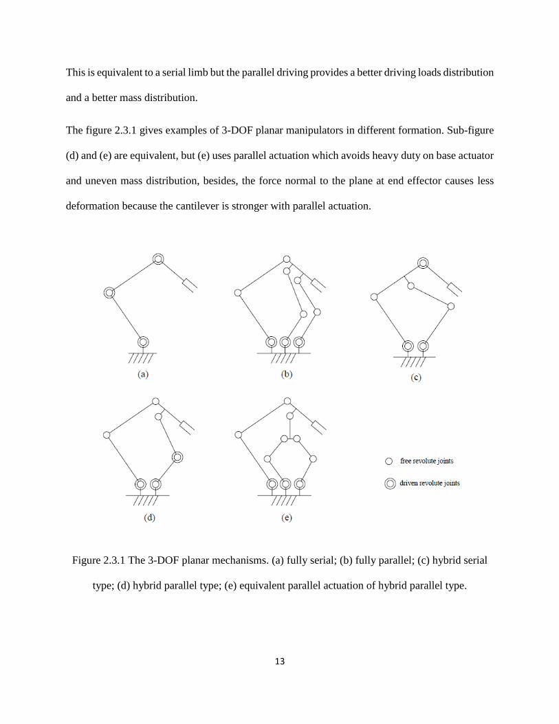
Figure 2.3.1 The 3-DOF planar mechanisms. (a) fully serial; (b) fully parallel; (c) hybrid

serial type; (d) hybrid parallel type; (e) equivalent parallel actuation of hybrid parallel type.

....................................................................................................................................................... 13

Figure 3.1.1 The shaking loads and balancing loads on a frame. ........................................... 23

Figure 3.2.1 Higher DOF manipulator with mobile vertical plane on horizontal planar

mechanism. .................................................................................................................................. 28

Figure 4.2.1 Planar (2-RR)R design. (a) convex; (b) concave. ................................................ 33

Figure 4.2.2 Spatial 3-RRS design. (a) convex; (b) concave. ................................................... 34

Figure 4.3.1 Mechanical design.................................................................................................. 35

Figure 4.3.2 Kinematic analysis. ................................................................................................ 37

Figure 4.3.3 First demonstration. (a) trajectory 1; (b) genetic algorithm optimization; (c)

driving torques original; (d) driving torques optimized; (e) power consumption index 𝑝𝑗 over

time; (f) energy consumption index 𝑓𝑗 over time. ................................................................... 47

Figure 4.3.4 Second demonstration. (a) trajectory 2; (b) genetic algorithm optimization; (c)


time; (f) energy consumption index 𝑓𝑗 over time. .................................................................... 48

Figure 4.4.1 3-RRS robot design. ............................................................................................... 51

Figure 4.4.2 3-RRS robot modelling. ......................................................................................... 52

Figure 4.4.3 Largest workspace by 𝑟𝑝, 𝑙𝑢, 𝑙𝑓 and 𝑧𝑏𝑖. ............................................................ 60

xii

Figure 4.4.4 The displacement of 𝜃𝑒𝑥, solid: original; dash: modified. ................................. 64

Figure 4.4.5 The displacement of 𝜃𝑒𝑦, solid: original; dash: modified. ................................. 64

Figure 4.4.6 The displacement of 𝑧𝑒, solid: original; dash: modified. ................................... 65

Figure 4.4.7 Energy index (𝑒)𝑗 increases over time, run 1, run 2, run 3. .............................. 65

Figure 4.4.8 The Simulink model of the manipulator in blocks. ............................................ 68

Figure 4.4.9 The Simulink model of the manipulator in 3D visualization window. ............. 69

Figure 4.4.10 The reaction torques −𝑇1, −𝑇2 and −𝑇3 sensor value and theoretical value.

....................................................................................................................................................... 70

Figure 4.4.11 The base reaction forces along 𝒙𝐨, 𝒚𝐨 and 𝒛𝐨 axes. ......................................... 71

Figure 4.5.1 The combination of balanced robots. ................................................................... 74

Figure 5.3.1 The 3-PRS parallel stand. (a) non-adaptive 3-PRS design; (b) storm protection

pose for non-adaptive design; (c) adaptive 3-PRS design; (d) storm protection pose for

adaptive design. ........................................................................................................................... 80

Figure 5.3.2 The structure for analysis. (a) the stand; (b) the rail and leg set. ..................... 81

Figure 5.3.3 Four parabola for seasonal division. .................................................................... 91

Figure 5.3.4 Optimization using pareto front. (a) winter; (b) fall/spring; (c) summer. ....... 93

Figure 5.3.5 Optimization results display. (a) workspace; (b) stiffness. ................................ 94

Figure 5.4.1 The hybrid harvester. (a) lie-flat configuration; (b) working configuration. .. 97

Figure 5.4.2 Inverse kinematic parallel structure. ................................................................... 98

Figure 5.4.3 Lie-flat vectors diagram. ..................................................................................... 100

xiii

Figure 5.4.4 Minimum platform height 𝑧𝑐. ............................................................................ 105

Figure 5.4.5 Leg stiffness. (a) loading and reaction forces; (b) elastic model; (c) Piezo chip

size; (d) loads on piezo chips. ................................................................................................... 110

Figure 5.4.6 Optimization. (a) genetic algorithm for larger workspace; (b) workspace

boundary, dash: original; solid: optimized. ............................................................................ 112

Figure 5.4.7 the 𝑧𝑐 position mapping with optimized working configuration. ................... 113

Figure 5.4.8 Stiffness mappings in prescribed motion range. (a) log(𝑘𝑥) N/m; (b) log(𝑘𝑦) N/m;

(c) log(𝑘𝑧) N/m; (d) stiffness 𝑘𝑥φ polar plot about φ𝑧 𝜃𝑥 = 0.4 and 𝜃𝑦 = −0.5 at working

configuration 𝑿 = [−0.1 − 0.1 − 0.1]. ................................................................................... 115

Figure 6.3.1 Serial actuation. ................................................................................................... 121

Figure 6.3.2 Parallel actuation. ................................................................................................ 122

Figure 6.3.3 Kinematics analysis. ............................................................................................ 124

Figure 6.3.4 Horizontal plane. ................................................................................................. 125

Figure 6.3.5 Interference detection. ......................................................................................... 129

Figure 6.3.6 Jacobian matrix analysis. .................................................................................... 131

Figure 6.3.7 Full workspace in 𝜽𝒆𝟏, 𝜽𝒆𝟐, 𝜽𝒆𝟑 of result 4. .................................................... 135

Figure 6.3.8 Stiffness mapping 𝜽𝒆 = 15 ∙ 𝜋18020 ∙ 𝜋18010 ∙ 𝜋180𝑇. .................................. 136

Figure 6.4.1 Mechanical design. (a) perpendicular planes form the pattern of a limb; (b)

3T2R parallel manipulator topology diagram; (c) the 3T2R parallel manipulator in working

posture; (d) lie-flat posture. ..................................................................................................... 141

xiv

Figure 6.4.2 Kinematics analysis. (a) the kinematic analysis; (b) the limbs in vertical planes

and horizontal planes; (c) links on horizontal planes projected on plane O; (d) links on plane

B. ................................................................................................................................................. 142

Figure 6.4.3 Interference detection. ......................................................................................... 146

Figure 6.4.4 Jacobian matrix analysis. .................................................................................... 147

Figure 6.4.5 Full workspace in 𝜽𝒆𝟏, 𝜽𝒆𝟐, 𝜽𝒆𝟑 of result 2. .................................................... 153

Figure 6.4.6 Stiffness mapping 𝜽 = 𝜃𝑦1𝜃𝑒1 = 20 ∙ 𝜋18010 ∙ 𝜋180 and 𝑧𝑒 = 0.3. ............. 154

Figure 7.4.1 A robotic system of balanced and deployable manipulators green energy

powered. ..................................................................................................................................... 163

1

Chapter 1 Introduction

1.1 Robotics

Robots are controlled machines. The English word “Robot” originates from Czech word “Robota”

which means forced labor. Czech writer Karel Čapek firstly used word “Robot” in his 1921 play

Rossum’s Universal Robots for mechanical men made and controlled to do work in factories. They

finally rebelled against their human masters [1]. Robotics is the science and technology of robots.

Since robotic science was introduced, it rapidly attracted research interests and grew broadly. Now

robots are widely used for many applications [2].

As influenced by science fictions and public media, general public more often may think of robots

as machines with human appearance that replace human labor. The robots that look like human

are humanoid robots [3]. However, the robots don’t necessarily have to look like human.

Jorge Angeles classified robots as mobiles and manipulators [4]. Mobile robots move around, such

as the four-legged walking robot, Big Dog [5], swimming robotic fish [6], winged flying robots

[7] and so on. The manipulators need to be installed on stage and are designed to reach to places

with a moving end effector like the arm and hand.

Usually a manipulator has three parts: a moving end effector, a base, and some links that connect

and actuate the end effector from the base. A moving or static object where the manipulator is

installed on could be considered as a base. Jonathan Hodgins designed a manipulator to be installed

on the bottom of drones [8]. Moritz Arns designed a dual functioning landing gear for the drones

[9]. The CANADARM was designed to be sent to work in space [10]. The manipulators could also

2

be installed on fixed base. Industrial robots [11] are set along the production line to work on the

work parts conveyed on the line.

Structures of the manipulators could be generally classified as serial and parallel. A serial robot

has its links connected from base to the moving end effector in series like an arm. The design is

straightforward and commonly seen. A planar serial robot is designed with three revolute joints

perpendicular to the plane which could move horizontally and longitudinally on the plane and

rotate as well [12]. A SCARA robot [13] adds one more joint to the three-mobility planar serial

robot and makes it move vertically.

Another kind of manipulator structure is parallel.

1.2 Parallel Robots

Dan Zhang gives a review of advanced parallel robots, and he develops comprehensive design and

analysis methodologies for parallel manipulators of multiple limbs and mobilities [14]. A limb is

a group of jointed links. The parallel manipulators have several limbs that connected in parallel

between two platforms. The fixed platform is the base, and the moving platform is the end effector.

An example of planar fully parallel manipulator [15] 3-RRR has three legs each with one actuator.

This robot has three mobilities that could move horizontally and longitudinally on a plane and

rotate.

Compared to serial manipulators, the parallel manipulators have higher stiffness, loading capacity,

operational precision, but smaller workspace. These structures are widely applied in many

industries, such as training, surgical, manufacturing and so on [16].

3

As parallel structure has high stiffness while serial structure has large workspace. The parallel

features and serial features could be integrated to design a hybrid manipulator [17] to take

advantages of both.

Historically there were quite some mechanisms or machines designed with parallel nature,

however D. Stewart firstly raised the awareness of parallel mechanism in academic research. Since

D. Stewart published a significant fully parallel structure in 1965 named Stewart platform that has

six mobilities [18], the researches on parallel robotic structures started to bloom.

In the kingdom of parallel manipulators, there are unique categories of designs. The parallel limbs

could be flexible, such as the cable driven parallel manipulators [19] where the flexible cables pull

and lift a moving platform. For some designs and applications, the moving platform doesn’t need

to be one rigid body. A configurable platform could be composed by more than one jointed body,

so that the platform could change its shape [20] [21] [22]. The limbs of the parallel manipulators

may not be individually connected between base and platform, for some structures have chains

that connect between two limbs [23] [24].

The parallel structures discussed in this dissertation are the ones that have one rigid platform (non-

configurable platform), have the limbs that are individual with no chains between them. The limbs

are considered as a group of rigid bodies jointed together (non-cable driven) in kinematics and

dynamics analysis. However, in stiffness analysis, the elasticity in actuated joints or deformable

bodies are considered.

4

1.3 Objectives of the Study

Here are some important problems in the studies of parallel manipulators for further

improvements.

The parallel manipulators contain a group of rigid bodies with mass and rotational inertia. When

the manipulator is moving, the acceleration of the mass and rotational inertia could cause inertia

loads. That could lead to vibration and noise. These loads are known as shaking forces and shaking

moments. The elimination of these loads is known as dynamic balancing [25]. The balancing

requires additional components which could have link interference and take more driving energy.

Methods need to be discussed to design balanced manipulators with easier control, improved

balancing performance, interference-free, optimized energy consumption, and larger workspace.

This problem is important as it is about the precision and energy-saving of manufacturing.

The outdoor stormy weathers or compact indoor manufacturing tasks require parallel manipulators

to be folded close to the base to protect the structure or to give space to other components. There

are some researches on foldable parallel manipulators designs, but these parallel structures are of

configurable platform. Parallel structures of non-configurable platform are demanded in

applications. The researches of foldable designs for non-configurable platform manipulators are

rare. The modification and re-design of some common parallel manipulators to be foldable need

be discussed and novel designs with this feature will be developed. This feature is worth research

awareness as it provides a protection for outdoor working machines in severe weathers.

The parallel manipulators have multiple limbs and these limbs are very close to each other. When

the manipulator is actuated, these limbs may collide or interfere. The distance between the limbs

need to be calculated to determine whether any two bodies may interfere with each other. The

5

interference detection of limbs could be complex and take time for analysis. Parallel structures

need to be designed with less opportunity of interference and quick detection for potential

interference. This is significant for parallel manipulators of higher mobilities since they contain

more links between the platform and the base than the ones of lower mobilities. This problem will

be discussed in the dynamically balanced manipulators and deployable manipulators.

1.4 Organization of the Dissertation

Chapter 1 gives a general knowledge of robotics and introduces the important problems the

research of this dissertation is going to solve.

Chapter 2 reviews the knowledge and researches that are relevant to the problems. This provides

the knowledge background to readers and it paves the way for the methods to be discussed in the

next chapter.

Chapter 3 discusses the research challenges, describes the problems in more details and suggests

the methods and theories that could be developed or used to address the problems.

Chapter 4 deals with designs of dynamically balanced parallel manipulators. It demonstrates the

dynamic balancing and energy optimization methods for a planar parallel mechanism and then

expands the methods to design and optimize a spatial dynamically balanced mechanism. Structural

adaption and motion planning are involved in the energy optimization. The dynamic modeling in

theory are verified by Simulink. It also discusses the further combination of two balanced

mechanisms to make a balanced manufacturing machine of higher mobilities. Chapter 4 is written

6

according to author’s papers on 2-DOF (2-RR)R [26] and 3-DOF 3-RRS [27], including materials

from the sources with adaptions.

Chapter 5 deals with re-designs of some common low-mobility parallel manipulators. It analyzes

the function that is designed to fold parallel mechanisms. It looks at the stormy weather protection

for solar panel in solar tracking and presents the designs that enable the mechanisms to lie down

flat to the floor when storm attacks the tracking field. The foldable designs are analysed for parallel

mechanisms with three mobilities (two rotations and one translation). Methods such as minimum

platform height and modified Jacobian matrix are developed to assist the analysis and evaluation

of the designs. Chapter 5 is written according to author’s papers on 3-DOF 3-PRS [28] and 3-DOF

3-RPS [29], including materials from the sources with adaptions.

Chapter 6 deals with novel designs of high-mobility parallel manipulators. It expands the foldable

mechanism designs to higher mobilities. The synthesis design methods and interference

avoidance/detection methods are researched. Modified Jacobian matrix is developed for these

structures. Chapter 6 is written according to author’s papers on 6-DOF 3-[(2-RR)UU] [30] and 5-

DOF PRPU/2-[(2-RR)UU] [31], including materials from the sources with adaptions.

Chapter 7 concludes the contribution of the dissertation and looks forward to future work.

7

Chapter 2 Literature Review

2.1 Synthesis Methodology

Tingli Yang et al [32] summarized the general process of manipulator design. As a manipulator is

designed to work within designed space, first the task space is given, then a design comes up with

a solution space, and finally the solution space is going to be optimized. The key factors of

topology are joints, the connection of links by joints, and the constraint a joint implies on the links.

The motion of links connected in series is the composition of the motions of these joints, while the

motion of platform connect to the base by a group of limbs in parallel is the intersection of the

motions of the limbs. A group of links connected in series is a single open chain unit. The single

open chain units are easy and simple to analyze and use for design. It is common to use single

open chain units as one of multiple limbs for a parallel manipulator.

Dan Zhang [14] developed tables of topologies for parallel manipulators with open chain units

based on the Chebychev-Grübler-Kutzbach criterion. He summarized in the table the number of

mobilities a topology could achieve with various possibilities of legs and joints combination. From

this table, he continues to develop the parallel structures with one more leg than mobilities, so the

extra leg could serve as an unactuated passive leg which enhances the stiffness and kinematic

analysis of the structures. A passive leg determines and provides decoupled motion when the other

legs have full mobilities of six because the motion of parallel limbs is the intersection of their

motions. A family of parallel manipulators are designed with the passive leg [33] [34] [35], where

the passive leg determines the total mobility of the parallel mechanisms considering the

8

intersection nature of the parallel mechanism motions. He also suggests the combination of

manipulators to work beyond the mobilities of individual robots that involve in the combination.

After a mechanism is designed, its mobility also known as degree of freedom (DOF) needs to be

determined. The formula developed based on Chebychev-Grübler-Kutzbach criterion are

simplified called G-K formula. The G-K formula could easily be used to determine the degree of

freedom based on number of links, number of joints, total mobilities of all joints [17].

A classical G-K formula is given below, where 𝑀 represents the degrees of freedom, C is 3 for

planar mechanism or 6 for non-planar mechanism, B is the number of bodies, J is the number of

joints, and ∑ 𝑑𝑖𝐽𝑖=1 represents the total degrees of freedom from all the joints in the mechanism.

𝑀 = C(B − J − 1) + ∑ 𝑑𝑖𝐽𝑖=1 (2.1.1)

Classical G-K formula is commonly known, and widely adopted by engineers and educators [36]

[37]. The G-K formula is easy to use and gives quick and correct solution for most of the cases.

However, in some special mechanisms, many researches discovered that the classical G-K formula

didn’t give correct solution for mobilities. For some circumstance, the G-K formula needs to be

modified for certain usages [38].

Zheng Huang et al [39] reviewed the 150 years of history seeking a unified formula for mobilities

(DOF). He concludes that G-K formula is not correct in all cases while a unified formula for

mobilities is not found yet. He suggested his research based on screw theory and he also classified

other categories of methods.

There is a category of methods based on Jacobian matrix [40]. Although Jacobian matrix is

complex, it does not increase the calculation work because Jacobian matrix is also needed for

9

stiffness mapping [41] which is commonly conducted to evaluate the deformation under loading.

The rank of the Jacobian matrix represents the mobility of the mechanism [42]. Some research

uses lie group theory to design a mechanism and then use Jacobian matrix to determine the

actuation joints [43]. This is an alternative of verifying mobility with Jacobian matrix.

After a designed mechanism has its mobility verified, a topology diagram and a notation in letters

with signs are needed to represent this structure. Network diagram [44] [45] of circles connected

by lines is common in representing structure, where the circles represent rigid bodies and the lines

represent the joints that connect the bodies. Another diagraming method [46] also takes the

network pattern but more specifically indicates the orientation of joints, which is not commonly

used. There are generally two notation methods to indicate the structure. One method [47] is

defining the structure by the output of end motion of platform in a given sequence (for example:

2R1T or 2T1R as the first or second types of Gf motion set). This method clearly shows the degree

of freedom and motions of the structure however doesn’t give details of how the links are

connected. Another method [14] is defining the joints in sequence from base to platform where the

numbers with hyphen followed by joints indicate the duplicate or identical chains in parallel (for

example 3-RRR or 6-UPS as the name and order of the joints connection where the underlined

joint is driven). For the cases when the limbs are not identical or when it is a hybrid limb, one

could consider using the notation in [48], where the bracket holds a part in serial connection and

slash indicate a non-identical chain is connected from base to platform in parallel (for example

RRR/(2-RRR)R is the notation for the structure in figure 2.3.1 (e)). This method indicates how the

links are connected but doesn’t give information on the motions at the end effector. One may need

to use both notations (end effector motion and links connection) to comprehensively describe a

structure. One needs to notice some joints could be combined to equal to another joint. For

10

example, RRR or RU when their rotation axis intersect at one point could be equal to spherical

joint. Sometimes, such replacement brings a better performance.

2.2 Family of 2R1T Manipulators

Newly developed structures may be uncertain in performance, which may need long term trial and

modification before commercial usage.

Family of 2R1T robots could make two rotations and one translation in any order. Some of the

examples have been developed long ago and already widely applied. It is safer to adopt or modify

the commonly known structures, as the relevant technical documents are abundant.

QinChuan Li et al [49] reviewed a group of parallel manipulators of 2R1T motion and classified

them into four categories according to the order of equivalent joint outputs from base to the moving

platform. These are the motions equivalent to UP, P*U*, PU and RPR. Most of the existent 2R1T

robots belong to one of the four types.

The UP type equals a universal joint and a prismatic joint connected in the given sequence. An

example is the Tricept robot with a passive leg to constraint the motion as UP [50].

The P*U* type is close to a prismatic joint and a universal joint connected in the given sequence

but with coupled translational motions. Examples are A3 and Z3 sprint heads for manufacturing

[51]. This type includes many well known and adopted structures such as 3-PRS, 3-RPS, 3-RRS

and so on.

11

The PU type equals to a prismatic joint and a universal joint connected in the given sequence.

There are some examples designed with a passive leg that constraints the moving platform as to

yield a PU output [52] [34] [53].

The PRP type equals to a prismatic joint, a revolute joint and another prismatic joint connected in

the given sequence. One example is the Exechon machine [54].

The research [49] further analyzed the designs with or without the constraining passive leg.

Theoretically the machines with constraining passive leg could output the motion equivalent to the

joints connected in series, while the ones without constraining passive leg yield coupled motions,

also known as parasitic motions. However, in reality, the platform has a thickness. For example,

the end effector of a PU type has a distance away from the center of the last joint on the

constraining leg, U joint. In other words, the platform centre is not exactly the joint center.

Optimization could minimize the deviation but could not eliminate it.

Researches [49] and [14] reviewed many examples of designs and suggested the trend in 2R1T

robot design. That leads to the combination of a 2R1T robot with a planar manipulator which has

at least two motions (the x and y axis motions on the plane). The merits of the combination are

first, to provides an offset to cancel the deviation motions in the 2R1T manipulator, and second,

to add at least two translational motions to make the pair of robots eligible for at least five degrees

of freedom.

There are plenty of common 2R1T structures. They could be modified to improve the performance.

12

2.3 Hybrid Structures

Dan Zhang [14] described the beauty of hybrid structures which integrate the parallel and serial

structures for the beneficial natures of both. The parallel robots have higher stiffness while the

serial robots have larger working space. Serdar Küçük [17] described the features of fully serial,

fully parallel and hybrid manipulators. Examples of planar 3-DOF mechanisms are given [55] in

fully serial, fully parallel and hybrid structures respectively.

As is summarized from review of many hybrid designs, there are mainly two types of hybridizing.

These are the serial type hybridizing and parallel type hybridizing based on the pattern of how sub-

mechanisms are connected into the manipulator.

The serial type hybridizing means connecting mechanisms or manipulators in series, just like the

serial manipulator that connects the links in series. For example, the parallel robots and serial

robots could be connected in series as in [55] [56]; and multiple parallel robots could be connected

in series [57]; a parallel robot and a single joint could be connected in series [58] [59].

The parallel type hybridizing means connecting limbs in parallel between the moving platform and

the base, where at least one limb contains at least two actuators. The limb that contains at least two

actuators is similar with serial mechanisms. For example, some 6-DOF manipulators are composed

of three limbs where each limb has links and joints connected in series and two joints of each limb

are driven [60] [61] [62] [63] [64] [65].

For when a limb has two actuated joints in series the actuated joint, closer to base, needs to carry

the load of the actuator in the middle of the limb. This requires more driving capability and larger

size of the base actuators. So that, some researches discuss the parallel type hybridizing with limb

that contains at least two driven joints, but the driving joints are in parallel [66] [48] [67] [68].

13

This is equivalent to a serial limb but the parallel driving provides a better driving loads distribution

and a better mass distribution.

The figure 2.3.1 gives examples of 3-DOF planar manipulators in different formation. Sub-figure

(d) and (e) are equivalent, but (e) uses parallel actuation which avoids heavy duty on base actuator

and uneven mass distribution, besides, the force normal to the plane at end effector causes less

deformation because the cantilever is stronger with parallel actuation.

Figure 2.3.1 The 3-DOF planar mechanisms. (a) fully serial; (b) fully parallel; (c) hybrid serial

type; (d) hybrid parallel type; (e) equivalent parallel actuation of hybrid parallel type.

14

The hybrid structures designed for higher degrees of freedom have a design merit which reduces

the chances of link interference [60] [62] [64] [69] [65] [67] compared to the equivalent fully

parallel counterparts, because the hybrid structures are simpler than equivalent fully parallel

structures. This reduces the chances of interferences and offers a larger workspace.

2.4 Redundancy and Adaption

Joints bring degrees of freedom to a mechanism, but the added DOF may not contribute to add

dimensions in end effector motions. For example, a serial open chain on a plane could at most

translate in x and y and rotate about z axes, while adding more prismatic joints on that plane

increases the DOF but doesn’t make it a spatial mechanism. When joints provide redundant

motions, they need to be locked or driven to eliminate idle motions. The redundancy describes this

feature of structure where the number of actuators exceeds the degrees of freedom [14].

Some works have reviewed the redundancy in parallel robot design [70] [71] [72] [73]. Among

the works, [72] has summarized that there are three types of redundancy. It gave the design process

for redundancy as 1) original non-redundant structure, 2) modification, 3) geometric parameters

to be chosen (set redundancy) to optimize some performances.

The three types of redundancy are described as following.

(a) Kinematic redundancy by definition [74] adds more degree of freedom through joints to the

limbs and it needs actuators to control the additional degree of freedom. Benefits and applications

are in eliminated singularity [75], improves dynamic performances [76] [77], optimized force

distribution [78], and reduced operational gap [79].

15

(b) Actuation redundancy by definition [80] [81] doesn’t add more degree of freedom but uses

actuators on originally passive joints or adds additional actuated limb(s). Benefits and applications

are in eliminated singularity, improved force and dynamic performances [82] [80] and tuned

natural frequency [83].

(c) Internal redundancy by definition [72] is the additional degree of freedom which allows some

mass to move for better dynamic performances, while the relative motion between the base and

the moving platform is not affected by this redundancy. The counter mass position is adjusted for

balancing [84]. Mass moving for balancing [85]. (See more examples in the active dynamic

balancers). Parallel robot dynamic performance can be improved by reconfiguration, known as re-

dyn [86] [87].

These types of redundancy are compared for their different properties. The actuation redundancy

adds constraint to the motion thus is more difficult to control. The internal redundancy may involve

additional motors and mass on a limb. The kinematic redundancy could be considered to allow

adaption in design.

The adaption [88] and reconfiguration [89] though the redundancy improves the performances.

The design could be modified from originally non-redundant structures for optimization.

2.5 Kinematics and Dynamics

Jorge Angeles [4] introduced transformation matrix for rigid body linear translation and angular

rotation as for the positions, instant velocity and acceleration.

16

The inverse kinematics is suitable for parallel manipulators to calculate positions, velocities and

accelerations. Such examples are the inverse kinematics analysis of planar 3-DOF 3-RRR parallel

mechanism [15] and 2R1T 3-RRS manipulator inverse kinematics and dynamics [90].

There are algebraic method and geometric method to calculate the Jacobian matrix.

The algebraic method usually takes the constant length of a link and develop symbolic equations

about the end effector motions for derivatives [14].

The geometric method uses vectors to represent the velocities of the links and develops a

relationship between the end effector and the actuators. For a translational and rotational rigid link,

the velocity could be simplified where only the velocity along the link needs to be equivalent at

the two joints of the links. Such simplification uses dot multiplication with the vector that goes

along the two points at the joints on the link [91] [92].

The relationship between the end effector velocity and the actuation velocity is needed to form a

Jacobian matrix [4] which could be used for stiffness calculation or other purpose such as degree

of freedom verification.

Once the inverse dynamics is conducted with acceleration from the end effector to the actuation,

the d’Alembert’s principle [93] could be applied which considers acceleration as the force with

mass and then by equilibrium formula the reacting forces, moments along with driving

requirements will be calculated. An example of such application in 3-PRPR planar robot is found

in [94].

The MATLAB Simulink software [95] provides the dynamic simulation for multi-body

mechanical systems, where the translational dynamics is simulated based on Newton’s equation

17

and the rotational dynamics is simulated based on Euler’s equation. The theoretical values could

be verified.

2.6 Trajectory and Interpolation

The motion of the manipulator end effector could be adjusted for optimized performances. There

are some examples of such applications, such as the motor reduces driving forces and driving

torques with an optimized motion planning [96], the operation time is saved with motion planning

[97] and [98].

The motion is adjusted by key points and needs interpolation methods to supply points between

two key points. An interpolation by splines is adopted to supply points at time interval for energy

optimization [99], another example uses Lagrange interpolation method for energy optimization

[100]. The polynomial interpolation is easy to use [101] as it conveniently offers high degree of

derivative equation to represent the displacement, velocity and acceleration.

A polynomial interpolation equation is given below, where 𝑠(𝑡𝑖) is a function of displacement

about time at 𝑡𝑖. The order of the interpolation equation depends on the number of conditions that

need to be met by the planned motion.

𝑠(𝑡𝑖) = 𝑚𝑛𝑡𝑖𝑛 + 𝑚𝑛−1𝑡𝑖

𝑛−1 + ⋯+ 𝑚0 (2.6.1)

𝑠(𝑡𝑖) = 𝑠𝑖, ��(𝑡𝑖) = 𝑣𝑖, ��(𝑡𝑖) = 𝑎𝑖 (2.6.2)

18

2.7 Optimization

The performances could be changed when some features or parameters are adjusted. They could

be adjusted to tune to the better performance. Such is known as the optimization.

The general aim of optimization is to find a global minimum [102] of an objective (cost function)

within the search area. E. K. P. Chong et al [103] introduced classical methods and other more

recent methods for optimization. For classical methods are not suitable for highly complex non-

linear cost functions, genetic algorithm (GA) is often used for complex cost functions.

Here is the cost function 𝑓𝑗 about the input variables 𝑥1, 𝑥2, ⋯ , 𝑥𝑛.

𝑓𝑗 = 𝑔𝑗(𝑥1, 𝑥2, ⋯ , 𝑥𝑛) (2.7.1)

The theory of genetic algorithm works as keeping only a group of best samples and mutating them

for next generation of competition [103]. The input variables are the adjustable features in a design

or a motion planning while the output is the cost function. Redundancy offers the room for

adjustment without affecting the overall degree of freedom of the manipulators.

In some situations, it is not only one cost function that needs to be optimized. Some multiple

objectives are sought together. The best result is not one single solution in these situations but are

a group of solutions that seek the best of an objective without sacrificing the other objectives. The

multi-objective optimization keeps a pareto front and updates the front in each generation [104].

In an example of two objective optimization, there are two cost functions, probably conflicting.

The two-objective optimal results are a group of results where either objective couldn’t be further

optimized without compromising the other objective. In this way, the two objectives are both at

their best fitness without sacrificing the other. Similarly, when more objectives are involved, the

19

optimization would yield a group of optimal results where each result represents the best of all

objectives before sacrificing any of the objective.

The aims in a design are usually multiple and conflicting. Multi-objective optimization yields a

group of optimal results. The results are considered as equally good if there is no preference on

selection of privileged objective. One needs to select from the optimal results for a solution with

most suitable combination of all objectives.

2.8 Chapter Conclusion

This chapter reviews the theories and general process in manipulator design from a design task to

a design solution/analysis and finally the opportunity for optimization. According to this process,

it navigates and introduces the knowledge in robotic structural design, modification, kinematic and

dynamic analysis, motion planning and finally optimization.

20

Chapter 3 Research Motivation and Methods

3.1 Research Motivations

Some common planar parallel manipulators such as (2-RR)R, and some common 2R1T spatial

parallel structures, such as 3-RRS, 3-PRS, 3-RPS, are widely employed in many industries.

However, there is room for improvement in their performances. These common structures need to

be modified, re-designed or combined to achieve better performance.

Novel structures are needed for special operation requirements. The designs need to be verified

for actual degrees of freedom and modified to come up with various DOF manipulators of similar

structure.

The improvement in dynamically balanced mechanisms and design of deployable manipulator are

sought, where link-interference need to be avoided and checked.

3.1.1 Dynamic Balancing

The moving centres of mass generate shaking forces and moment which could cause vibration and

noise. The dynamic balancing of robots is to improve the unbalanced conditions of robots and to

eliminate the shaking forces and moments during motion [25].

Dan Zhang and Bin Wei [105] [106] [107] [108] classified the balancing methods in two types.

They are 1) balancing before synthesis and 2) balancing after synthesis. Many designs and methods

21

are reviewed under the two types of balancing strategies. The main difference is the priority

between balancing and functional requirements.

1) Balancing before synthesis is reviewed in paper [109]. This method, by definition, deals with

balancing first and then composes a structure with balanced sub-mechanisms. The design examples

are: a planar four bar mechanism [110] and a design of 6-DOF mechanism with three legs each is

a balanced 3-DOF balanced mechanism [111]. The adjustment of design may be difficult.

2) Balancing after synthesis is more straightforward. This method, by definition, deals with design

to satisfy the needs of functions and then adds balancing parts. An example is the planar 2-DOF

manipulator which is designed for its function first and then it is added with counterweights for

balancing [86] [112]. The adjustment of design is easier.

The balancing could be achieved by passive and active means.

Passive means include adding counter inertia [86] [112], reconfiguration that converts part of the

functioning body to balancing mass [105], or sometimes optimal adjustment that is not seeking a

complete balancing but reduced shaking forces and moments [113] [114] [84].

Active means include motion planning and driven balancers. Some designs are aimed at producing

counter forces and counter moments under control to cancel out the shaking forces and shaking

moments, such as a 3-DOF planar balancer [115] and a 6-DOF full balancer [116] designed to be

attached to unbalanced sources.

Some designs integrate the passive and active balancing means together. A planar 3-RRR

manipulator has counterweights attached to the legs so that the centre of mass is stationary while

the shaking moment is balanced by an actively driving flywheel [117]. A group of 1-DOF, 2-DOF

22

and 3-DOF planar mechanisms are designed with passive counterweight force balancing and active

rotation for moment balancing [118].

One needs to consider the nature and property of different balancing means.

The passive balancing needs to attach counter mass on each leg. However, high-DOF parallel

manipulator has multiple legs so that the counter mass may require more installation space which

could leads to interference and smaller workspace. Furthermore, the passive balancing assumes

that the load is constant during operation. Tasks such as pick-and-place could not be completely

balanced by passive balancing. The passively balanced multiple legs for higher degrees of freedom

may have higher collision or interference chances, thus may need to be avoided. Instead, the

combination of two balanced low degrees of freedom mechanisms could be a replacement. And

unnecessary weight on legs or on platform should be avoided in passive balancing design, because

this will multiply the counter mass weight on legs and takes more energy. For this reason, serial

type hybridizing should be avoided since the weight on platform is largely increased although the

workspace is large. The passive means is mainly applied in force balancing.

Active balancing increases the control difficulties because the real-time calculation of shaking

loads is difficult. Besides, there will be local deformation or local unbalance between the shaking

loads source and balancing loads. For this reason, active balancers need to be located where they

could isolate the shaking source from the working table. (see figure 3.1.1)

23

Figure 3.1.1 The shaking loads and balancing loads on a frame.

According to the above analysis, passive and active balancing means are recommended to be

integrated for better balancing effects, such as passive force balancing and active moment

balancing for manipulators with revolute joints. The shaking forces are passively balanced at the

revolute joints while the sensing and real-time calculation of shaking moments at the driven joints

are relatively easy as for the active moment balancer. Link interference and energy consumption

need more research as additional balancing components are required for dynamic balancing.

Motion planning should be considered when allowed. For balanced operation in higher mobilities,

the combination of two lower degrees of freedom mechanism could be considered.

24

3.1.2 Deployable Structures

The challenging outdoor weathers such as storms could damage the structure especially when the

structure has a large face that takes the wind loads. The storms are frequent in tropical regions

[119]. In North America, solar panels destroyed by storms are heard in news or website [120]

[121]. Besides the weather, the indoor compact manufacturing space may also require the structure

to be folded to give way to other machines or workpieces that pass by.

The design that could be folded are known as deployable structures. The recent research shows the

design of 1-DOF deployable platform which is used for lifting [122]. And another research shows

the design of multi-DOF configurable platform with deployable feature [22]. In both cases, the

limbs are in fixed vertical planes, perpendicular to the base.

There are some structures that have the potential to be modified as deployable parallel robots, but

the development for deployable feature is not discussed in these designs yet. A serial arm is

connected to the platform of a parallel manipulator whose limbs are in fixed vertical planes [56],

so that the lower parallel stage could be folded. The 2T1R family of three-limb HALF [123] and

HANA parallel robots [124] have the limbs in three fixed vertical planes. The 6-DOF 3-RUPU

parallel manipulator [125] which has limb in mobile vertical planes. The sealion robots [60] are

designed with 4-DOF, 5-DOF and 6-DOF which have the limbs in mobile vertical planes. In three

leg robots with more than three degrees of freedom, the limb has at least two actuators. When the

actuators are arranged in series, one actuator will take the weight of the other actuator. However,

when legs are increased, there may be a small workspace or interference problem. The RHHR [67]

is a design with two parallel actuations in each limb for a 6-DOF 3-leg parallel robot. This kind of

25

integrated joint is newly developed of which more data on its performance might be published in

the future.

The research for multi-DOF non-configurable platform deployable parallel structure is rare. Some

common designs of parallel manipulators, such as those from the 3-DOF 2R1T family, have non-

configurable platform. They need to be re-designed for the deployable feature in applications

where this feature is needed.

While 2R1T parallel manipulators are re-designed for deployable feature, the design method could

be expanded to design higher-DOF deployable parallel manipulators. Using the modified G-K

formula to make a disseminated G-K formula and applying the motion sets intersection for parallel

structure, one could choose the end effector motions for the design through the main limb. Finally,

the degrees of freedom need to be verified with Jacobian matrix for its rank. This doesn’t increase

development process as Jacobian matrix is needed also for stiffness calculation.

3.1.3 Link Interference

The parallel manipulators have several limbs. They have chances of colliding with each other

(internal interference) or colliding with external objects (external interference). The interferences

need to be avoided. This dissertation will analyze the link interference (internal interference). It is

significant to reduce the chances of the link to link interferences as this affects the volume of

workspace [126] [127] [128]. The pose should be interference free when evaluating or optimizing

the workspace.

When links are modeled as line-segments, one needs to calculate the shortest distance between

two line-segments. The distance between two line-segments in a certain degree of space is given

26

in [129], where the relative orientations and arrangements of the two line-segments need to be

discussed and sorted in some cases for further discussion. However, the links are not line-

segments, because they have width and thickness. Some researches have modeled the links as

cylinders with a radius [130] [127] [131], and the distance calculation depends the relative

orientations and arrangements of the two cylinders. The algorithms are based on discussion in

categories.

Besides the interference detection algorithms, some design methods can avoid interference. As is

researched in [132], the 3-RRR spherical parallel manipulator design proposes three design tips to

avoid interference. And [133] also concludes that multiple layers, link shapes, joint replacements

as the methods to avoid interferences.

The methods and relevant design examples are given in the following.

(a) modify link shape on the same layer [133].

(b) put links on difference planes.

(b.1) the planes (layers) are parallel to each other [134].

(b.2) the planes are intersecting.

(b.2.1) the intersecting planes are perpendicular to the moving platform, such as in 6-DOF 3-[(2-

RR)SR] [66] or 6-DOF 3-USR [62].

(b.2.2) the intersecting planes are perpendicular to the base, such as in 3-DOF 3-RRS or 6-DOF 3-

[(2-RR)UU].

27

(c) some special joint such as RHHR [67] that contains two non-conflicting motions. This example

is also applicable in (b.2.2). The RU pair of joints [135] is designed to have a larger motion range

and is equivalent to a spherical joint which is usually limited in motion range [136].

When design and its workspace are determined, motion planning is also an option to avoid link to

link interference [137].

Large number of links in three-dimensional space take longer time in interference detection. The

design should avoid link interferences where possible and make detection easier. The design and

detection methods will be discussed on 2R1T manipulators and higher-DOF parallel manipulators.

The high-DOF manipulator could arrange the limbs in different vertical planes or parallel layers

to reduce the changes of interference while making the detection easier.

3.2 Design Methods

Considering the needs for dynamic balancing, deployable feature and interference avoidance, the

parallel robots with limbs in vertical planes satisfy these requirements.

The 2R1T 3-RRS parallel manipulator could offer 2 rotations and 1 translation and ideal for force

balancing with the revolute joints. The moments are balanced by flywheels above the 3-RRS, so

the area under the 3-RRS robot is free from shaking forces and shaking moments. With a

combination to a balanced planar parallel manipulator, they could form a pair of large workspace

balanced manufacturing machine. The planar balanced parallel structure could be 3-RRR or (2-

RR)R, because the revolute joints are ideal for force balancing and they could have an active driven

28

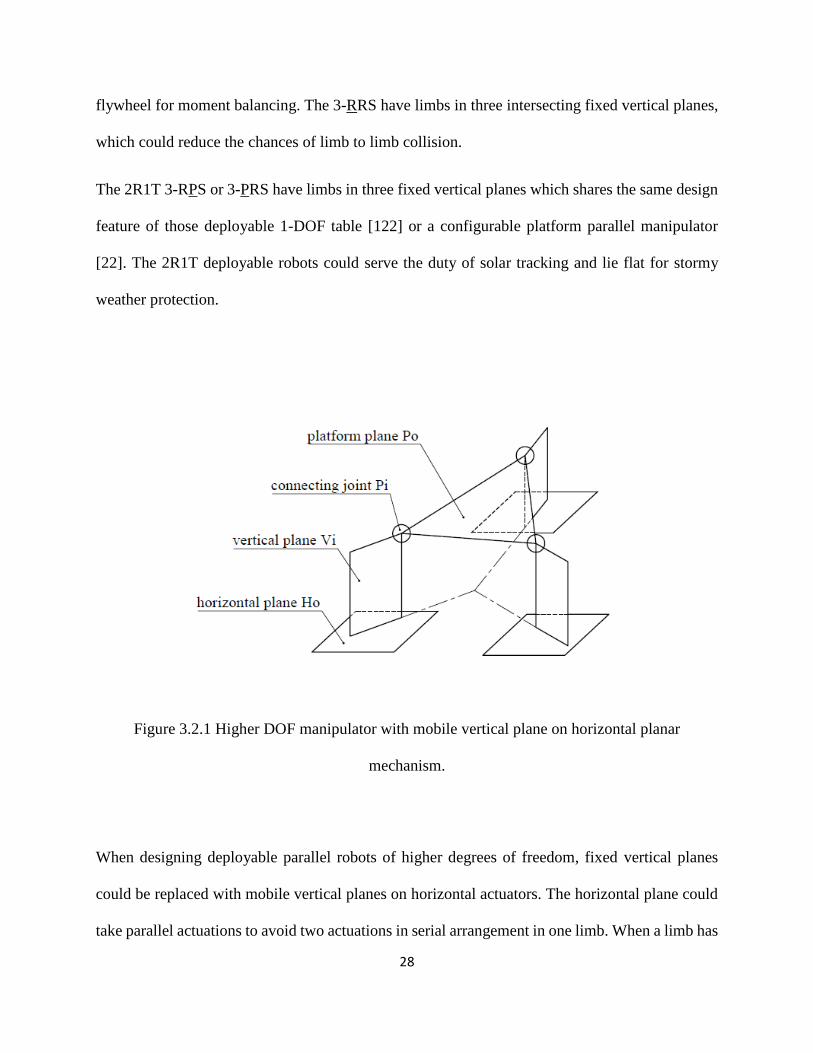
flywheel for moment balancing. The 3-RRS have limbs in three intersecting fixed vertical planes,

which could reduce the chances of limb to limb collision.

The 2R1T 3-RPS or 3-PRS have limbs in three fixed vertical planes which shares the same design

feature of those deployable 1-DOF table [122] or a configurable platform parallel manipulator

[22]. The 2R1T deployable robots could serve the duty of solar tracking and lie flat for stormy

weather protection.

Figure 3.2.1 Higher DOF manipulator with mobile vertical plane on horizontal planar

mechanism.

When designing deployable parallel robots of higher degrees of freedom, fixed vertical planes

could be replaced with mobile vertical planes on horizontal actuators. The horizontal plane could

take parallel actuations to avoid two actuations in serial arrangement in one limb. When a limb has

29

two actuators, the design could put all actuation weights on the base. The loads and actuation duty

need to be evenly distributed, and the limb needs to be tough in holding weight. Therefore, serial

type hybrid manipulator is not considered; for parallel type hybrid manipulators, the two actuators

are aligned in parallel on base for each limb.

3.3 Evaluation Methods

The design is going to be evaluated for performances such as workspace volume, stiffness and

energy consumption.

The workspace volume is to be evaluated with inverse kinematics by finding the eligible end

effector positions. For solar tracking applications with 2R1T manipulators where the translational

motion is redundant, minimum platform height algorithm (intersection of possible solutions) is

developed that could rapidly search for eligible workspace for 2R1T solar trackers. In high-DOF

manipulators, where the horizontal actuations are arranged in parallel layers, only eligible pose

without interference could be counted to evaluate workspace. The boundary offset method is

developed for same layer interference scan.

General stiffness summation is taken as an overall evaluation index for stiffness in multiple

directions [14]. Modified Jacobian matrix 𝑱𝒆 is derived from classical Jacobian matrix 𝑱𝒐 for

stiffness evaluation in directions other than the global coordinate axes.

𝑲𝒐 = 𝑱𝒐𝑇𝑲𝒒𝑱𝒐 , 𝑱𝒐𝒙�� = �� (3.3.1)

𝑲𝒆 = 𝑱𝒆𝑇𝑲𝒒𝑱𝒆, 𝑱𝒆𝒙�� = �� (3.3.2)

30

Energy index is taken to evaluate the energy consumption where many articles are taking actuation

force squared or torque squared as the index of energy consumption [138] [139] [140].

3.4 Applications and Optimizations

The following chapters will present the designs and analysis of adaptive (2-RR)R or (2-RR)R

balanced robot and 3-RRS balanced robot where the dynamic balancing and optimal energy

consumption problem will be discussed through structural adaptive features and motion planning.

Furthermore, the two balanced manipulators are combined for higher DOF balanced operations.

The adaptive 3-PRS and 3-RPS robots from the 2R1T family are re-designed for applications as

deployable solar trackers and multiple objectives are optimized. The deployable design has been

expanded to higher degree of freedom, where hybrid parallel manipulator with limbs in mobile

vertical planes on horizontal actuations are discussed and the designs are optimized for multiple

objectives.

The design objectives can be larger workspaces with given platform orientations, minimum sizes

and minimum lie-flat height, while operational objective can be minimum energy consumption,

and higher stiffness dependant on what are demanded in a certain task which may be different from

task to task. The design objectives usually take structural sizes as inputs to the optimization

problem, while the operation objectives usually take adaptive variables as inputs to the

optimization problem. Therefore, the optimizations in many cases are practiced in two stage. The

first stage is a design optimization to decide design parameters (for example, the geometric sizes

of links). Once these sizes are decided, they become fixed sizes. The second stage is an operational

optimization that takes advantages of the kinematic redundancy or structural adaptive features of

31

a design to find an adjustment that is optimal to a certain task. Both design or operational

optimizations could be single-objective or multi-objective. But they would be better to be done in

two stages. If both design parameters and the adaptive parameters are optimized together, the

computation time may be exponentially increased.


The motivation is to design various DOF dynamically balanced or deployable parallel

manipulators with less link interference. Structures with limbs in vertical planes satisfy the

requirements. This includes arranging the parallel limbs in fixed vertical planes (3-DOF 2R1T

manipulators) or mobile vertical planes with parallel actuations on horizontal plane (higher DOF

manipulators). The horizontal planes could be arranged in layers to avoid interference.

Minimum platform height algorithm, link boundary offset, modified Jacobian matrix, and torque

squared are the methods that evaluate the performances of the design. When the performances

have room for further improvement, the structure could be adapted, or best design parameters

could be found through single or multi objective optimization.

The applications are manufacturing and energy harvesting. The designs will be demonstrated in

the following chapters.

32

Chapter 4 Dynamic Balancing for Various DOF Motions

4.1 Chapter Introduction

The moving inertia of unbalanced machine brings about shaking forces and shaking moments

which could cause vibration and noise. Finally, it affects the precision of manufacturing. Dynamic

balancing is demanded to provide a solution.

This chapter discusses the dynamic balancing of common parallel manipulators by passive force

balancing and active moment balancing, because the motor torques are easier to be actively sensed

and balanced. Due to the additional balancing components, it has possibility of link interference

and takes more energy to drive the system. The configuration change is suggested in the design

for interference avoidance. Structural adaption and motion planning are discussed for energy

consumption minimization.

A first example of an adaptive planar 2-DOF (2-RR)R parallel mechanism is demonstrated, where

the effect of adaption alone is examined for minimizing the driving energy. This machine can be

modified to be a 3-DOF (2-RR)R balanced planar mechanism by serial type hybridizing.

A second example is an adaptive 2R1T 3-DOF 3-RRS parallel mechanism. The effect to minimize

driving energy is compared between structure adaption alone and structure adaption with motion

planning. The theoretic dynamic model is verified by Simulink software.

Finally, the combination of the two machines, (2-RR)R and 3-RRS, for a dynamically balanced 6-

DOF manufacturing machine is discussed.

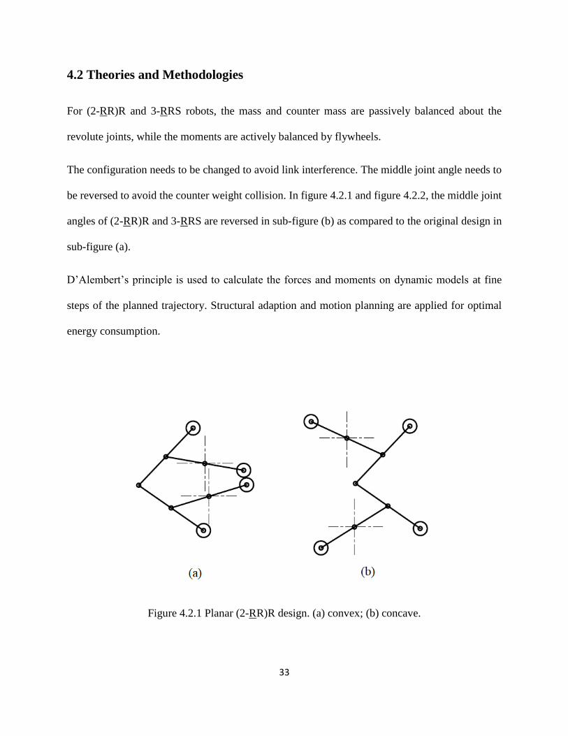
33

4.2 Theories and Methodologies

For (2-RR)R and 3-RRS robots, the mass and counter mass are passively balanced about the

revolute joints, while the moments are actively balanced by flywheels.

The configuration needs to be changed to avoid link interference. The middle joint angle needs to

be reversed to avoid the counter weight collision. In figure 4.2.1 and figure 4.2.2, the middle joint

angles of (2-RR)R and 3-RRS are reversed in sub-figure (b) as compared to the original design in

sub-figure (a).

D’Alembert’s principle is used to calculate the forces and moments on dynamic models at fine

steps of the planned trajectory. Structural adaption and motion planning are applied for optimal

energy consumption.

Figure 4.2.1 Planar (2-RR)R design. (a) convex; (b) concave.

34

Figure 4.2.2 Spatial 3-RRS design. (a) convex; (b) concave.

4.3 Planar Dynamic Balancing

This section presents a dynamically balanced planar parallel manipulator, (2-RR)R robot, with

structurally adaptive design which can be adjusted to minimize the overall energy consumption

required to complete a defined cyclic motion of the end effector. The genetic algorithm is adopted

to search for optimal adaption that results to minimum energy consumption. The (2-RR)R robot

discussed in this section has shaking forces passively balanced by counter masses, and the shaking

moments actively balanced by a flywheel. A balanced mechanism eliminates noise and vibration

however may require additional driving energy due to its additional balancing components. As for

a defined motion that ought to be repeated in cycles, adaption could be an energy saving strategy

when alternating the motion is not applicable.

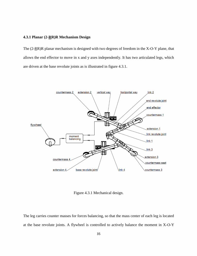
35

4.3.1 Planar (2-RR)R Mechanism Design

The (2-RR)R planar mechanism is designed with two degrees of freedom in the X-O-Y plane, that

allows the end effector to move in x and y axes independently. It has two articulated legs, which

are driven at the base revolute joints as is illustrated in figure 4.3.1.

Figure 4.3.1 Mechanical design.

The leg carries counter masses for forces balancing, so that the mass center of each leg is located

at the base revolute joints. A flywheel is controlled to actively balance the moment in X-O-Y

36

plane. Each base revolute joint is mounted on a stage that is able to adjust its position along the

horizontal (x axis) and vertical (y axis) ways, which changes dynamic properties. Industrial

engineers can reposition the input joints based on the defined motion of the end effector. These

stages will be locked from moving once the positions of the base revolute joints are determined.

During the end effector motion, the adaption is locked so that the input joints positions are fixed.

The structure can be written in full as (2-PPRR)R.

4.3.2 Inverse Kinematics and Dynamics

The (2-RR)R robot is a rigid parallel robot thus the inverse kinematics method is practiced to

calculate the mechanism pose from a given end effector position (figure 4.3.2 (a)). The rigidity

applies to the velocity and acceleration calculations (figure 4.3.2 (b)).

The input revolute joints are at 𝑩𝟏 and 𝑩𝟐, and the end effector at position 𝑷. The positions are

represented by vectors from coordinate origin 𝑶. There are two identical legs, where 𝑖 = 1 𝑜𝑟 2

represents the index of leg.

𝑶𝑩i = [𝑥𝑏i 𝑦𝑏i 0]𝑇, 𝑶𝑷 = [𝑥𝑝 𝑦𝑝 0]𝑇 (4.3.1)

With these vectors, the angular displacements of the input joints are calculated.

𝜃𝑖 = 𝑡𝑎𝑛−1 (𝑦𝑝−𝑦𝑏𝑖

𝑥𝑝−𝑥𝑏𝑖) + [−1]𝑖 cos−1 (

|𝑩i𝑷|2+𝑙22−𝑙1

2

2∙|𝑩i𝑷|𝑙2) (4,3.2.a)

Where,

|𝑨𝐢𝑷| = |𝑨𝐢𝑫𝐢| = 𝑙1 and |𝑨𝐢𝑩𝐢| = |𝑩𝐢𝑪𝐢| = 𝑙2 (4.3.2.b)

The positions of revolute joints 𝑨𝟏 and 𝑨𝟐 are given below.

37

𝑶𝑨i = 𝑶𝑩i + 𝑙2[cos𝜃𝑖 sin𝜃𝑖 0]𝑇 (4.3.3)

Figure 4.3.2 Kinematic analysis.

The values of the angular displacements need to be judged to determine if the given end effector

position 𝑷 is reachable. Only eligible pose is considered for further analysis.

The velocity relationship between the end effector and the input joints are given.

𝝎𝑩i × 𝑩i𝑨i + 𝝎𝑨i × 𝑨i𝑷 = 𝒗𝒑 (4.3.4.a)

Since the end effector has two degrees of freedom, its velocity has components along x axis and y

axis. The angular velocities of the two links on each leg are obtained.

𝝎𝑩i = [0 0 ��i]𝑇 , 𝝎𝑨i = [0 0 ��ai]

𝑇 (4.3.4.b)

38

The angular velocities of the links are needed in acceleration analysis.

The angular acceleration of the links can be calculated through the end effector acceleration.

𝒂𝑨𝒊 = 𝜶𝑩i × 𝑩i𝑨i + 𝝎𝑩i2𝑨i𝑩i (4.3.5.a)

𝒂𝑩𝒊 = 𝟎 (4.3.5.b)

𝒂𝑪𝒊 = −𝒂𝑨𝒊 (4.3.5.c)

The acceleration of point 𝑷 is 𝒂𝒑.

𝒂𝒑 = 𝒂𝑨𝒊 + 𝜶𝑨i × 𝑨i𝑷 + 𝝎𝑨i2𝑷𝑨i (4.3.5.d)

𝒂𝑫𝒊 = 2𝒂𝑨𝒊 − 𝒂𝒑 (4.3.5.e)

Since the end effector has two degrees of freedom, its acceleration 𝒂𝒑 has components along x

axis and y axis. The angular accelerations of the two links on each leg are obtained.

𝜶𝑩i = [0 0 ��i]𝑇 , 𝜶𝑨i = [0 0 ��ai]

𝑇 (4.3.5.b)

The inertias need to be given to determine loads and actuation forces.

Counter mass 1, 𝑚𝑑1, is at point 𝑫𝟏; counter mass 2, 𝑚𝑐1, is at 𝑪𝟏; counter mass 3, 𝑚𝑑2, is at point

𝑫𝟐; counter mass 4, 𝑚𝑐2, is at 𝑪𝟐; and the end effector mass, 𝑚𝑝, is at point 𝑷. These are modeled

as concentrated masses.

The four rotating bodies of the (2-RR)R robot are aligned with vectors 𝑫𝟏𝑷, 𝑫𝟐𝑷, 𝑨𝟏𝑪𝟏 and 𝑨𝟐𝑪𝟐,

have masses noted as 𝑚𝑎1, 𝑚𝑎2, 𝑚𝑏1, and 𝑚𝑏2 respectively, excluding the counter masses and the

end effector mounted on them. These masses are modeled as evenly distributed along the vectors

with the center of mass at the rotating axis of the bar.

39

For the links 𝑫𝐢𝑷, since |𝑨𝐢𝑫𝐢| = |𝑨𝐢𝑷|, if 𝑚𝑑i =1

2𝑚𝑝, the centripetal forces and the tangential

forces are cancelled. For the links 𝑪𝐢𝑨𝐢, since |𝑩𝐢𝑨𝐢| = |𝑩𝐢𝑪𝐢|, if 𝑚𝑐𝑖 =1

2𝑚𝑝 + 𝑚𝑑𝑖 + 𝑚𝑎𝑖, the

centripetal forces and the tangential forces are cancelled. The whole (2-RR)R robot is completely

force balanced.

Rotational inertia of links 𝑷𝑫i about revolute joint 𝑨𝒊 with all masses loaded on it is denoted as 𝐼𝑎𝑖.

𝐼𝑎𝑖 =1

12𝑚𝑎𝑖(2𝑙1)

2 + 𝑚𝑑𝑖𝑙12 +

1

2𝑚𝑝𝑙1

2 (4.3.6.a)

Rotational inertia of links 𝑪i𝑨i about revolute joint 𝑩𝒊 with all masses loaded on it is denoted

as 𝐼𝑏𝑖.

𝐼𝑏𝑖 =1

12𝑚𝑏𝑖(2𝑙2)

2 + 2𝑚𝑐𝑖𝑙22 (4.3.6.b)

At the revolute joint of end effector 𝑃, the two legs are connected. A force 𝑭𝒑 acts on link |𝑨𝟏𝑷|,

its reaction force −𝑭𝒑 acts on link |𝑨𝟐𝑷|. The mutual forces form the moments around joint 𝑨1

and 𝑨2 which cause the angular accelerations.

One could consider adding a rotation to the 2-DOF motion by adding a rotary motor that exerts a

moment 𝑴𝒑 around z axis on link |𝑨𝟏𝑷|. The output torque of this motor is 𝑻𝒑 = −𝑴𝒑. This

makes it a 3-DOF planar hybrid mechanism. If there is no extra motor added, then 𝑴𝒑 = 𝟎.

𝑨1𝑷 × 𝑭𝒑 + 𝑴𝒑 = 𝐼𝑎1𝜶𝑨𝟏, (4.3.7.a)

𝑨2𝑷 × (−𝑭𝒑) = 𝐼𝑎2𝜶𝑨𝟐 (4.3.7.b)

The forces 𝑭𝑨𝟏 and 𝑭𝑨𝟐 act on links |𝑨𝟏𝑷| and |𝑨𝟐𝑷| respectively.

𝑭𝒑 + 𝑭𝑨𝟏 − 𝑚𝑎1𝒂𝑨𝟏 − 𝑚𝑑1𝒂𝑫𝟏 −1

2𝑚𝑝𝒂𝒑 = 𝟎 (4.3.7.c)

40

−𝑭𝒑 + 𝑭𝑨𝟐 − 𝑚𝑎2𝒂𝑨𝟐 − 𝑚𝑑2𝒂𝑫𝟐 −1

2𝑚𝑝𝒂𝒑 = 𝟎 (4.3.7.d)

The forces 𝑭𝑩𝒊 act on links |𝑩𝐢𝑨𝐢| from the base joint 𝑩𝐢.

𝑭𝑩𝒊 − 𝑭𝑨𝒊 − 𝑚𝑐𝑖𝒂𝑪𝟏 = 𝟎 (4.3.7.e)

As the forces are balanced for both legs, only moments are remained to be balanced. The driving

torques around the input joints 𝑩1 and 𝑩2 are given as below.

𝑻𝐢 = 𝑩i𝑨i × 𝑭𝑨𝒊 + 𝐼𝑏𝑖𝜶𝑩𝒊 (4.3.8.a)

The third torque 𝑻𝟑 is controlled to balance the overall moment on the base.

𝑻𝟏 + 𝑻𝟐 + 𝑻𝟑 = 𝟎 (4.3.8.b)

The energy consumption of direct current electric motor consists the mechanical energy and the

heat loss [141]. For each of the three motors in the balanced (2-RR)R robot, the supplied power is

formed by two parts as described in the equation below.

U𝑖I𝑖 = E𝑖I𝑖 + I𝑖2𝑅 , i=1, 2 or 3 (4.3.9.a)

The back electromagnetic force is proportional to the rotating speed of the input joints, where 𝐾𝑒

is a constant parameter of the motor.

E𝑖 = 𝐾𝑒𝜔𝑖 , i=1, 2 or 3 (4.3.9.b)

The current is proportional to the torque exerted around the input joints, where 𝐾𝑡 is a constant

parameter of the motor.

Ii = Kt(𝐳 ∙ 𝐓𝐢) , i=1, 2 or 3 (4.3.9.c)

The mechanical energy consumption is from the back electromagnetic force and the current.

41

E𝑖I𝑖 = 𝐾𝑒Kt𝜔𝑖(𝐳 ∙ 𝐓𝐢) (4.3.9.d)

The rest of the energy consumption is the heat loss which is proportional to the current squared.

As the current is proportional to torque, the heat loss is proportional to the torque squared.

I𝑖2𝑅 = Kt

2R𝐓𝐢2 (4.3.9.e)

The acceleration of the input joints consumes electric energy while the braking by reversing plugs

generates electric energy [142], which is reflected in the back electromagnetic force. The (2-RR)R

robot is accelerating and braking during the cycle of motion. If the friction is not considered during

the motion, the energy consumption is the total heat loss on the resistances of the motors, which is

proportional to current squared. Current squared, or torque squared, has been considered as the

rate of energy consumption based on algorithm in [138] [139] [140]. The integration of the rate

over time is the total energy consumption of the robot.

Torques 𝑻𝟏 and 𝑻𝟐 act at joints 𝑩1 and 𝑩2; 𝑻𝟑 acts on the flywheel for moment balancing. Power

𝑃𝑖 is proportional to torque 𝐓𝐢 squared.

𝑃𝑖 = I𝑖2𝑅 ∝ 𝐓𝐢

2𝑅 (4.3.9.f)

4.3.3 Operation Optimization of Energy Consumption Index

Since the dynamic properties change as the positions 𝑩𝟏 and 𝑩𝟐 are relocated, a single-objective

optimization is run for optimal 𝑩𝟏 and 𝑩𝟐 positions that lead to least energy consumption for a

prescribed motion.

With the design parameters given in table 4.3.1, the dynamic simulation can be performed in

MATLAB.

42

Table 4.3.1 The (2-RR)R robot design parameters.

Symbols Units Values

𝑚𝑝 kg 0.2

𝑚𝑑i kg 0.1

𝑚𝑐i kg 0.3

𝑚𝑎𝑖 kg 0.1

𝑚𝑏𝑖 kg 0.1

𝑙1 m 0.2

𝑙2 m 0.2

The end effector travels in cycles along a close-loop trajectory that is 𝐿 in length. Each cycle takes

period time 𝑇 to travel. 𝑇 is evenly divided to n pieces of steps, each with an index number j. The

magnitude of velocity |𝒗𝒑| is constant. At each step marked by j, the kinematic and dynamic index

are calculated with respect to time.

Table 4.3.2 Trajectory parameters.

Parameters Values

𝐿 0.36 𝑚

𝑇 3.6 𝑠

𝑛 360

|𝒗𝒑| 0.1 𝑚/𝑠

Starting point [0.0 0.1 0.0]

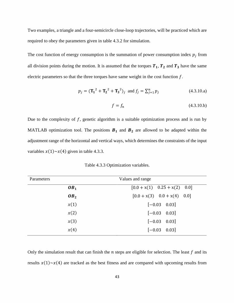
43

Two examples, a triangle and a four-semicircle close-loop trajectories, will be practiced which are

required to obey the parameters given in table 4.3.2 for simulation.

The cost function of energy consumption is the summation of power consumption index 𝑝𝑗 from

all division points during the motion. It is assumed that the torques 𝑻𝟏, 𝑻𝟐 and 𝑻𝟑 have the same

electric parameters so that the three torques have same weight in the cost function 𝑓.

𝑝𝑗 = (𝐓𝟏2 + 𝐓𝟐

2 + 𝐓𝟑2)𝑗 and 𝑓𝑗 = ∑ 𝑝𝑗

𝑛𝑗=1 (4.3.10.a)

𝑓 = 𝑓𝑛 (4.3.10.b)

Due to the complexity of 𝑓, genetic algorithm is a suitable optimization process and is run by

MATLAB optimization tool. The positions 𝑩𝟏 and 𝑩𝟐 are allowed to be adapted within the

adjustment range of the horizontal and vertical ways, which determines the constraints of the input

variables 𝑥(1)~𝑥(4) given in table 4.3.3.

Table 4.3.3 Optimization variables.

Parameters Values and range

𝑶𝑩𝟏 [0.0 + x(1) 0.25 + x(2) 0.0]

𝑶𝑩𝟐 [0.0 + x(3) 0.0 + x(4) 0.0]

𝑥(1) [−0.03 0.03]

𝑥(2) [−0.03 0.03]

𝑥(3) [−0.03 0.03]

𝑥(4) [−0.03 0.03]

Only the simulation result that can finish the 𝑛 steps are eligible for selection. The least 𝑓 and its

results 𝑥(1)~𝑥(4) are tracked as the best fitness and are compared with upcoming results from

44

trials. This will only be replaced once better fitness is found. The optimization terminates after all

generations of candidates are attempted.

Trajectory 1 parameters are given in table 4.3.4. The trajectory is a close-loop triangle. The

points 𝐾0, 𝐾1 and 𝐾2 are the three vertices of the triangle. The end effector starts the motion at 𝐾0

then moves to 𝐾1, and then 𝐾2, finally returns to 𝐾0 when a cyclic motion is complete.

Table 4.3.4 Trajectory 1 parameters.

Parameters Values

𝑶𝑲𝟎 [0.0 0.10 0.0]

𝑶𝑲𝟏 [0.9 0.22 0.0]

𝑶𝑲𝟐 [0.9 0.10 0.0]

The trajectory 1, and the results are plotted in figure 4.3.3. The values of original and optimized

results are given in table 4.3.5 for trajectory 1.

Table 4.3.5 Original and optimized results of trajectory 1.

Parameters Original values Optimized values

x(1) 0.0 -0.028

x(2) 0.0 0.029

x(3) 0.0 0.03

x(4) 0.0 -0.03

𝑓 0.375 0.12538

Optimization efficiency 1-0.12538/0.375=66.57%

45

Trajectory 2 parameters are given in table 4.3.6. The trajectory is a close-loop with four semi-

circles. The points 𝑶𝟏, 𝑶𝟐, 𝑶𝟑 and 𝑶𝟒 are the centers of the semi-circles with radius 𝑅1, 𝑅2, 𝑅3

and 𝑅4 respectively. The first semi-circle route is from 𝜋 to 0 clockwise; the second semi-circle

route is from 𝜋 to 2𝜋 counter clockwise; the third semi-circle route is from 𝜋 to 2𝜋 counter

clockwise; the fourth semi-circle route is from 2𝜋 to 𝜋 clockwise. The end effector starts from the

first semi-circle route, then second semi-circle route, then third semi-circle route, finally the fourth

semi-circle route and returns to the starting point of the first semi-circle route.

Table 4.3.6 Trajectory 2 variables.

Parameters Values

𝑅1 0.12 𝜋⁄

𝑅2 0.06 𝜋⁄

𝑅3 0.15 𝜋⁄

𝑅4 0.03 𝜋⁄

𝑶𝑶𝟏 [0.12 𝜋⁄ 0.0 0.0]

𝑶𝑶𝟐 [0.30 𝜋⁄ 0.0 0.0]

𝑶𝑶𝟑 [0.21 𝜋⁄ 0.0 0.0]

𝑶𝑶𝟒 [0.03 𝜋⁄ 0.0 0.0]

The trajectory 2, and the results are plotted in figure 4.3.4. The values of original and optimized

results are given in table 4.3.7 for trajectory 2.

46

Table 4.3.7 Original and optimized results of trajectory 2.

Parameters Original values Optimized values

x(1) 0.0 0.029

x(2) 0.0 0.03

x(3) 0.0 0.022

x(4) 0.0 -0.029

𝑓 8.8623 5.5890

Optimization efficiency 1-5.5890/8.8623=36.94%

For trajectory 1, joint relocation is able to save 66.57% of energy within constraints. For trajectory

2, joint relocation is able to save 36.94% of energy. If both trajectories are to be repeated in large

number of cycles as in production line operations, the saving in energy is remarkable.

47

Figure 4.3.3 First demonstration. (a) trajectory 1; (b) genetic algorithm optimization; (c) driving

torques original; (d) driving torques optimized; (e) power consumption index 𝑝𝑗 over time; (f)

energy consumption index 𝑓𝑗 over time.

48

Figure 4.3.4 Second demonstration. (a) trajectory 2; (b) genetic algorithm optimization; (c)


time; (f) energy consumption index 𝑓𝑗 over time.

49

4.3.4 Re-design to be (2-RR)R for Planar 3-DOF Operation

At the end effector, a driven rotation could be added to make it a 3-DOF planar hybrid manipulator.

The balancing weight and balancing moment are to be adjusted accordingly.

4.3.5 Section Conclusion

The dynamically balanced (2-RR)R robot is free from vibration and noise problems, however it

has additional mass and balancing components which cause the machine to be more energy-

consuming. Through repositioning its input joints on the base, the energy consumption can be

minimized without the need to change the motion of end effector. Two trajectory examples with

defined motion have been conducted and the optimization efficiency is obvious. The optimization

effect is dependent on trajectories. This method may effectively save energy for robots that repeat

a given cyclic motion and it is easy to adopt. Its applications may be developed in automated

manufacturing plants that largely rely on robots, as to promote an energy saving and environmental

friendly production. This mechanism could be re-designed by adding an actuator at the end effector

to make a 3-DOF (2-RR)R planar mechanism.

4.4 Spatial P*U* Dynamic Balancing

This section discusses the adaptive relocation of a manipulator joints and motion planning as

methods to reduce energy consumption in robotic manipulators. A 3-RRS dynamically balanced

parallel manipulator is designed for manufacturing operations and on which numerical simulations

50

is practiced for demonstration. The dynamically balanced manipulator contains additional

balancing components and requires additional energy in actuation which makes energy problem

significant. It promotes environment-friendly green operations of manipulators in energy saving

through optimization of adaptive joint locations in supplement to motion planning, meanwhile it

eliminates vibration and noise problems by dynamic balancing.

4.4.1 A 3-RRS Mechanism Design

In figure 4.4.1, the 3-RRS is composed of three identical sets of arms that hold the platform and

move it in 3D space. Each arm is actuated by the motor which is seated in the motor box. Each

arm has two links which are the up arm and the fore arm. The up arm is driven by the rotary motor.

The fore arm is a follower which is connected to the up arm with a revolute joint and is connected

to the platform with a spherical joint. Counter masses are attached to arms on their extension parts

to locate centers of gravity at revolute joints to achieve passive force balancing. The total moment

needs to be actively balanced by flywheels which are actuated by two motors on the roof top in

two orthogonally aligned axes. The height of each motor box is adjustable and self-locking by the

vertical lead screw. The structure can be written in full as 3-PRRS.

51

Figure 4.4.1 3-RRS robot design.

52

Figure 4.4.2 3-RRS robot modelling.

4.4.2 Inverse Kinematics and Dynamics

The inverse kinematics and dynamics [4] [90] is employed for position, velocity and dynamic

analysis.

In figure 4.4.2, each arm is set in a fixed plane. The rotation matrix 𝑸𝒊 about axis 𝒛𝒐 that transforms

from 𝒙𝒐𝑶𝒛𝒐 to 𝒙𝒊𝑶𝒊𝒛𝒊, coordinate system of each plane, is given below. Let 𝑖 (𝑖 = 1,2,3) be the

index of the three arms.

53

𝑸𝒊 = [𝑐𝑜𝑠𝛼𝑖 −𝑠𝑖𝑛𝛼𝑖 0𝑠𝑖𝑛𝛼𝑖 𝑐𝑜𝑠𝛼𝑖 0

0 0 1] (4.4.1.a)

The 𝒆𝒙, 𝒆𝒚 and 𝒆𝒛 are unit vectors parallel to the global coordinate axes 𝒙𝒐, 𝒚𝒐, and 𝒛𝒐 respectively.

𝒆𝒙 = [ 1 0 0]𝑇, 𝒆𝒚 = [ 1 0 0]𝑇, 𝒆𝒛 = [ 1 0 0]𝑇 (4.4.1.b)

The actuated rotational joints are in position 𝑩𝒊.

𝑶𝑩𝒊 = [ 𝑟𝑏cos𝛼𝑖 𝑟𝑏sin𝛼𝑖 𝑧𝑏𝑖]𝑇 (4.4.2)

The 3-RRS manipulator has 3 DOFs. The platform has its center at point 𝑬 which has two

orientation motions 𝜃𝑒𝑥, 𝜃𝑒𝑦 , (𝜃𝑒𝑧 = 0), and three linear motions 𝑥𝑒, 𝑦𝑒, 𝑧𝑒. The variables 𝜃𝑒𝑥,

𝜃𝑒𝑦, 𝑧𝑒 are independent motions, while 𝑥𝑒, 𝑦𝑒 are following motions.

The orientation of the platform is given as rotation matrix 𝑹 in global coordinate. Its rotation angle

𝜃𝑒 = √𝜃𝑒𝑥2 + 𝜃𝑒𝑦

2 is around unit axis vector 𝑼𝒆 = [𝑢𝑥 𝑢𝑦 0]𝑇, where 𝑢𝑥 =

𝜃𝑒𝑥

𝜃𝑒, 𝑢𝑦 =

𝜃𝑒𝑦

𝜃𝑒

[143].

𝑹 = [

𝑐𝜃𝑒 + 𝑢𝑥2(1 − c𝜃𝑒) 𝑢𝑥𝑢𝑦(1 − c 𝜃𝑒) 𝑢𝑦𝑠𝜃𝑒

𝑢𝑥𝑢𝑦(1 − c 𝜃𝑒) 𝑐𝜃𝑒 + 𝑢𝑦2(1 − c𝜃𝑒) −𝑢𝑥𝑠𝜃𝑒

−𝑢𝑦𝑠𝜃𝑒 𝑢𝑥𝑠𝜃𝑒 𝑐𝜃𝑒

] (4.4.3.a)

The triangle platform has three vertices 𝑷𝒊 that 𝑶𝑷𝒊 = 𝑹𝒊 + 𝑶𝑬 is perpendicular to the 𝒚𝒊 axis,

where 𝑹𝒊 = 𝑹 ∙ [𝑟𝑝cos𝛼𝑖 𝑟𝑝sin𝛼𝑖 0]𝑇. Therefore 𝑥𝑒 and 𝑦𝑒 from 𝑶𝑬 = [𝑥𝑒 𝑦𝑒 𝑧𝑒]𝑇 are

calculated.

(𝑸𝒊𝒆𝒚) ∙ 𝑶𝑷𝒊 = (𝑸𝒊𝒆𝒚) ∙ (𝑹𝒊 + 𝑶𝑬) = 0 (4.4.3.b)

54

The rotation angles 𝜃𝑎𝑖 𝜃𝑏𝑖 are calculated on each set of arms accordingly, and the solution needs

to satisfy kinematic criteria to be an eligible solution.

𝜃𝑎𝑖 = −cos−1 (𝑸𝒊𝒆𝒙)∙𝑨𝒊𝑷𝒊

𝑙𝑓 (4.4.3.c)

𝜃𝑏𝑖 = 𝜋 − 𝛽𝑏𝑖 − 𝜑𝑏𝑖 (4.4.3.d)

where,

𝛽𝑏𝑖 = cos−1 (𝑙𝑢

2+|𝑩𝒊𝑷𝒊|−𝑙𝑓2

2𝑙𝑢|𝑩𝒊𝑷𝒊|) (4.4.3.e)

𝜑𝑏𝑖 = sin−1 ((𝑩𝒊𝑷𝒊)∙𝒆𝒚

|𝑩𝒊𝑷𝒊|) (4.4.3.f)

The positions of 𝑨𝒊, 𝑪𝒊 and 𝑫𝒊 are calculated as below.

𝑶𝑨𝒊 = 𝑶𝑩𝒊 + 𝑸𝒊 [ cos𝜃𝑏𝑖

0 sin𝜃𝑏𝑖

] 𝑙𝑢 (4.4.4.a)

𝑶𝑪𝒊 = 𝑶𝑩𝒊 +𝑙𝑢𝑏

𝑙𝑢𝑨𝒊𝑩𝒊 (4.4.4.b)

𝑶𝑫𝒊 = 𝑶𝑨𝒊 +𝑙𝑓𝑏

𝑙𝑓𝑷𝒊𝑨𝒊 (4.4.4.c)

The compliant angle at joint 𝑨𝒊 from 𝒙𝒊 axis in 𝑶𝒊 coordinate is calculated.

𝜃𝑎𝑖 = −cos−1 [𝑨𝒊𝑷𝒊]𝑜𝑖∙𝒆𝒙

𝑙𝑓 (4.4.4.d)

Some criteria need to be satisfied. Only meaningful results are selected from pose solution to

avoid singularity and collision.

Criteria 1 judges whether a real solution of pose can be obtained.

55

𝑙𝑢 + 𝑙𝑓 > |𝑩𝒊𝑷𝒊| (4.4.5.a)

Criteria 2 ensures that links are never aligned so as to avoid singularity.

[𝑨𝒊𝑩𝒊 × 𝑨𝒊𝑷𝒊]𝑜𝑖 ∙ 𝒆𝒚 > 0 (4.4.5.b)

Criteria 3 ensures that the arms be above the platform surface so as to avoid singularity.

𝒏𝒆 = 𝑹𝟏 × 𝑹𝟐 (4.4.5.c)

𝑷𝒊𝑨𝒊 ∙ 𝒏𝒆 > 0 (4.4.5.d)

Criteria 4 ensures 𝑫𝒊 keep a distance from the 𝒛𝒐 axis as to avoid arms collision.

[𝑶𝑫𝒊 − 𝑶𝑫𝒊 ∙ 𝒆𝒛 ∙ 𝒆𝒛]𝑜𝑖 ∙ 𝒆𝒙 > 𝑑𝑚𝑖𝑛 (4.4.5.f)

Criteria 5 limits actuation angle within operational range.

𝜃𝑏𝑖 > 𝜃𝑚𝑖𝑛 (4.4.5.g)

Criteria 6 ensures that 𝑫𝒊 is under ceiling, or is above ceiling but not touching the ceiling.

𝑶𝑫𝒊 ∙ 𝒆𝒛 < ℎ𝑐 (4.4.5.h)

or,

𝑒𝑥𝑡𝑖 [𝑷𝒊𝑨𝒊

|𝑷𝒊𝑫𝒊|]𝑜𝑖

∙ 𝒆𝒙 > 𝑟𝑐 (4.4.5.i)

where,

𝑒𝑥𝑡𝑖 =ℎ𝑐−𝑶𝑷𝒊∙𝒆𝒛

(𝑷𝒊𝑫𝒊 |𝑷𝒊𝑫𝒊|⁄ )∙𝒆𝒛 (4.4.5.j)

Criteria 7 ensures that 𝑷𝒊 is above the production line surface.

56

𝑶𝑷𝒊 ∙ 𝒆𝒛 > 𝑧𝑚𝑖𝑛 (4.4.5.k)

Once the criteria for eligible pose are given, an optimization is run for largest workspace in defined

boundary. To reduce the overall machine weight by design, let balancing arm be in same length as

operation arm.

The linear velocity of point 𝑷𝒊 is 𝒗𝒑𝒊 which has a relationship with 𝒗𝒆 = [��𝑒 ��𝑒 ��𝑒]𝑇 and 𝝎𝒆 =

[��𝑒𝑥 ��𝑒𝑦 ��𝑒𝑧]𝑇, 𝒗𝒑𝒊 = 𝝎𝒆 × 𝑹𝒊 + 𝒗𝒆. The velocity 𝒗𝒑𝒊 is perpendicular to the 𝒚𝒊 axis.

(𝑸𝒊𝒆𝒚) ∙ 𝒗𝒑𝒊 = (𝑸𝒊𝒆𝒚) ∙ (𝝎𝒆 × 𝑹𝒊 + 𝒗𝒆) = 0 (4.4.6)

Also, the linear velocity of 𝑷𝒊 can be expressed by the angular velocities at joints 𝑨𝒊 and 𝑩𝒊, as

𝒗𝒑𝒊∗. The angular velocities 𝝎𝒂𝒊 = ��𝑎𝑖 ∙ 𝒚𝒊 and 𝝎𝒃𝒊 = ��𝑏𝑖 ∙ 𝒚𝒊 can be calculated.

𝒗𝒑𝒊∗ = 𝝎𝒃𝒊 × 𝑩𝒊𝑨𝒊 + 𝝎𝒂𝒊 × 𝑨𝒊𝑷𝒊 (4.4.7)

(𝑸𝒊𝒆𝒙) ∙ 𝒗𝒑𝒊 = (𝑸𝒊𝒆𝒙) ∙ 𝒗𝒑𝒊∗ (4.4.8.a)

(𝑸𝒊𝒆𝒛) ∙ 𝒗𝒑𝒊 = (𝑸𝒊𝒆𝒛) ∙ 𝒗𝒑𝒊∗ (4.4.8.b)

The linear acceleration of point 𝑷𝒊 is 𝒂𝒑𝒊 which has a relationship with 𝒂𝒆 = [��𝑒 ��𝑒 ��𝑒]𝑇 and

𝜶𝒆 = [��𝑒𝑥 ��𝑒𝑦 ��𝑒𝑧]𝑇, 𝒂𝒑𝒊 = 𝜶𝒆 × 𝑹𝒊 + 𝝎𝒆 × (𝝎𝒆 × 𝑹𝒊) + 𝒂𝒆. Acceleration 𝒂𝒑𝒊 is

perpendicular to the 𝒚𝒊 axis.

(𝑸𝒊𝒆𝒚) ∙ 𝒂𝒑𝒊 = (𝑸𝒊𝒆𝒚) ∙ [𝜶𝒆 × 𝑹𝒊 + 𝝎𝒆 × (𝝎𝒆 × 𝑹𝒊) + 𝒂𝒆] = 0 (4.4.9)

Also, the linear acceleration of 𝑷𝒊 can be expressed by the angular acceleration at joints 𝑨𝒊 and 𝑩𝒊,

as 𝒂𝒑𝒊∗. The angular accelerations 𝜶𝒂𝒊 = ��𝑎𝑖 ∙ 𝒚𝒊 and 𝜶𝒃𝒊 = ��𝑏𝑖 ∙ 𝒚𝒊 can be calculated.

𝒂𝒑𝒊∗ = 𝒂𝒂𝒊 + 𝜶𝒂𝒊 × 𝑨𝒊𝑷𝒊 + 𝝎𝒂𝒊 × (𝝎𝒂𝒊 × 𝑨𝒊𝑷𝒊) (4.4.10.a)

57

𝒂𝒂𝒊 = 𝜶𝒃𝒊 × 𝑩𝒊𝑨𝒊 + 𝝎𝒃𝒊 × (𝝎𝒃𝒊 × 𝑩𝒊𝑨𝒊) (4.4.10.b)

(𝑸𝒊𝒆𝒙) ∙ 𝒂𝒑𝒊 = (𝑸𝒊𝒆𝒙) ∙ 𝒂𝒑𝒊∗ (4.4.11.a)

(𝑸𝒊𝒆𝒛) ∙ 𝒂𝒑𝒊 = (𝑸𝒊𝒆𝒛) ∙ 𝒂𝒑𝒊∗ (4.4.11.b)

The angular accelerations 𝜶𝒄𝒊 and 𝜶𝒅𝒊 are in 𝒚𝒊 axis.

𝒂𝒄𝒊 = 𝜶𝒃𝒊 × 𝑩𝒊𝑪𝒊 + 𝝎𝒃𝒊 × (𝝎𝒃𝒊 × 𝑩𝒊𝑪𝒊) (4.4.11.c)

𝒂𝒅𝒊 = 𝒂𝒂𝒊 + 𝜶𝒂𝒊 × 𝑨𝒊𝑫𝒊 + 𝝎𝒂𝒊 × (𝝎𝒂𝒊 × 𝑨𝒊𝑫𝒊) (4.4.11.d)

In similar way, the accelerations of the counter masses would be obtained accordingly.

One could apply D’Alembert’s principle for force and moment analysis [93]. The mass 𝑚𝑒, 𝑚𝑝,

𝑚𝑑, and 𝑚𝑐 are concentrated at points 𝑬, 𝑷𝒊, 𝑫𝒊 and 𝑪𝒊. The mass 𝑚𝑎 and 𝑚𝑏 are evenly spread

along links 𝑷𝒊𝑫𝒊 and 𝑨𝒊𝑪𝒊. The inertia 𝐽𝑎 and 𝐽𝑏 are rotational around revolute joints at 𝑨𝒊 and 𝑩𝒊.

The force 𝑭𝒆 and the moment 𝑴𝒆 are the overall force and overall moment acting on the platform,

by the inertia.

𝑭𝒆 = ∑ [(𝒂𝒑𝒊 − 𝒂𝒈)𝑚𝑝]𝑚𝑖=1 + (𝒂𝒆 − 𝒂𝒈)𝑚𝑒 (4.4.12.a)

𝑴𝒆 = ∑ [𝑹𝒊 × (𝒂𝒑𝒊 − 𝒂𝒈)𝑚𝑝]𝑚𝑖=1 (4.4.12.b)

Force 𝑭𝒑𝒊 that acts on the platform at point 𝑷𝒊 from the arms causes the overall reaction 𝑭𝒆 and

𝑴𝒆 on platform.

𝑭𝒆 = ∑ 𝑭𝒑𝒊𝑚𝑖=1 (4.4.12.c)

𝑴𝒆 = ∑ [𝑹𝒊 × 𝑭𝒑𝒊]𝑚𝑖=1 (4.4.12.d)

58

The moment on the fore arm is balanced about joint 𝑨𝒊.

[𝑨𝒊𝑷𝒊 × (−𝑭𝒑𝒊)]𝑜𝑖∙ 𝒆𝒚 = [𝑨𝒊𝑫𝒊 × (𝒂𝒅𝒊 − 𝒂𝒈)𝑚𝑑 + 𝜶𝒂𝒊 ∙ 𝐽𝑎]

𝑜𝑖∙ 𝒆𝒚 (4.4.13.a)

The force on the fore arm is also balanced. The force 𝑭𝒂𝒊 is from up arm to fore arm.

𝑭𝒂𝒊 = 𝑭𝒑𝒊 + (𝒂𝒅𝒊 − 𝒂𝒈)𝑚𝑑 + (𝒂𝒂𝒊 − 𝒂𝒈)𝑚𝑎 (4.4.13.b)

The forces on up arm is balanced.

𝑭𝒃𝒊 = 𝑭𝒂𝒊 + (𝒂𝒄𝒊 − 𝒂𝒈)𝑚𝑐 − 𝒂𝒈𝑚𝑏 (4.4.13.c)

The force and moment acting on the fore arms and the up arms shall be balanced with the inertia

and acceleration given or obtained from above, at 𝑨𝒊 and 𝑩𝒊. The actuation torques 𝑻𝒊 are

calculated. 𝜶𝒃𝒊 is the angular acceleration about revolute joint at 𝑩𝒊. The magnitude value of the

𝑻𝒊 is 𝑇𝑖.

𝑻𝒊 = −(𝑸𝒊𝒆𝒚) ∙ (𝑩𝒊𝑨𝒊 × 𝑭𝒂𝒊) − (𝑩𝒊𝑪𝒊 × (𝒂𝒄𝒊 − 𝒂𝒈)𝑚𝑐) − 𝜶𝒃𝒊𝐽𝑏 (4.4.14.a)

𝑇𝑖 = 𝑸𝒊𝒆𝒚 ∙ 𝑻𝒊 (4.4.14.b)

The total moment on base the frame should be balanced with 𝑻𝒃, thus the total moment on base

the frame would be zero at all time.

𝑻𝒃 = −(𝑻𝟏 + 𝑻𝟐 + 𝑻𝟑) (4.4.14.c)

The balancing moment 𝑻𝒃 should be output by the two balancers (flywheels) in 𝒙𝒐 and 𝒚𝒐 axes

respectively.

𝑇𝑏𝑥 = 𝑻𝒃 ∙ 𝒆𝒙 (4.4.14.d)

59

𝑇𝑏𝑦 = 𝑻𝒃 ∙ 𝒆𝒚 (4.4.14.e)

Mechanical energy and the heat loss constitute the total energy consumption of a DC motor. The

transformation is reversible between electric energy and mechanical energy. When the friction is

neglected, the energy consumption is solely the heat loss on the electric resistances of the DC

motors which is reflected by the actuation torque squared, accumulated over operation time. The

instant power 𝑷𝒊 is proportional to actuation torque 𝐓𝐢 squared.

𝑃𝑖 = I𝑖2𝑅 ∝ 𝐓𝐢

2𝑅 (4.4.14.f)

4.4.3 Design Optimization

An optimization for largest workspace is conducted for the design based on the parameters given

in table 4.4.1 which considers the manipulator’s space requirements.

Over the expected search area for the three motions of the end effector which are 𝜃𝑒𝑥 [-1.5, 1.5],

𝜃𝑒𝑦 [-1.5, 1.5], 𝑧𝑒 [0.5, 1.0], the design parameters are optimized from their evaluated ranges.

Table 4.4.2 gives the results of the optimization for largest workspace.

Table 4.4.1 Design parameters.

Variables Units Values

𝑟𝑏 m 1.0

𝑟𝑐 m 0.3

ℎ𝑐 m 2.0

𝛼1 rad 0.75π/3

𝛼2 rad 2.75π/3

𝛼3 rad 4.75π/3

60

Table 4.4.2 Optimization constraints and results.

Parameters Units Ranges Results

𝑟𝑝 m [0.05, 0.1] 0.07

𝑙𝑢 m [0.2, 1.0] 0.79

𝑙𝑓 m [0.2, 1.0] 0.733

𝑧𝑏𝑖 m [1.0, 1.7] 1.394

The 𝑟𝑝, 𝑙𝑢, 𝑙𝑓 are the non-adjustable design parameters, while 𝑧𝑏𝑖 is an adjustable parameter that

could be adapted thus its value obtained here would be considered as a default value for largest

workspace. The result of the workspace is visualized with an enclosed convex hull in figure 4.4.3.

Figure 4.4.3 Largest workspace by 𝑟𝑝, 𝑙𝑢, 𝑙𝑓 and 𝑧𝑏𝑖.

61

4.4.4 Operation Optimization of Energy Consumption Index

In table 4.4.3, the end effector travels a trajectory where the three motions 𝜃𝑒𝑥, 𝜃𝑒𝑦 and 𝑧𝑒 are each

expressed in a unique polynomial function, with displacement 𝑠(𝑡), velocity ��(𝑡) and acceleration

��(𝑡). In table 4.4.3, the optimization variables are 𝑥1~𝑥12, where 𝑥1~𝑥3 set the adaptive

relocations of 𝑩𝒊 by 𝑧𝑏𝑖. The key points of time 𝑡0~𝑡6 are set in the column. At 𝑡0, 𝑡2 and 𝑡4, the

displacement and velocity allow no alteration at all. At 𝑡1, 𝑡3, 𝑡5, motion planning is optionally

allowed with 𝑥4~𝑥12.

𝑠(𝑡) = 𝑎12𝑡12 + 𝑎11𝑡

11 + ⋯+ 𝑎1𝑡1 + 𝑎0𝑡

0 (4.4.15)

Table 4.4.3 Trajectory features of 𝜃𝑒𝑥, 𝜃𝑒𝑦 and 𝑧𝑒.

𝑡0 𝑡1 𝑡2 𝑡3 𝑡4 𝑡5 𝑡6

𝑡 0 1 2 3 4 5 6

𝜃𝑒𝑥(𝑡) 0 𝑥4 0.7 𝑥5 -0.5 𝑥6 0

��𝑒𝑥(𝑡) 0 NA 0.2 NA 0.2 NA 0

��𝑒𝑥(𝑡) 0 NA NA NA NA NA 0

𝜃𝑒𝑦(𝑡) 0 𝑥7 -0.8 𝑥8 -0.6 𝑥9 0

��𝑒𝑦(𝑡) 0 NA -0.4 NA 0.3 NA 0

��𝑒𝑦(𝑡) 0 NA NA NA NA NA 0

𝑧𝑒(𝑡) 0.5 𝑥10 0.6 𝑥11 0.7 𝑥12 0.5

��𝑒(𝑡) 0 NA 0.1 NA -0.1 NA 0

��𝑒(𝑡) 0 NA NA NA NA NA 0

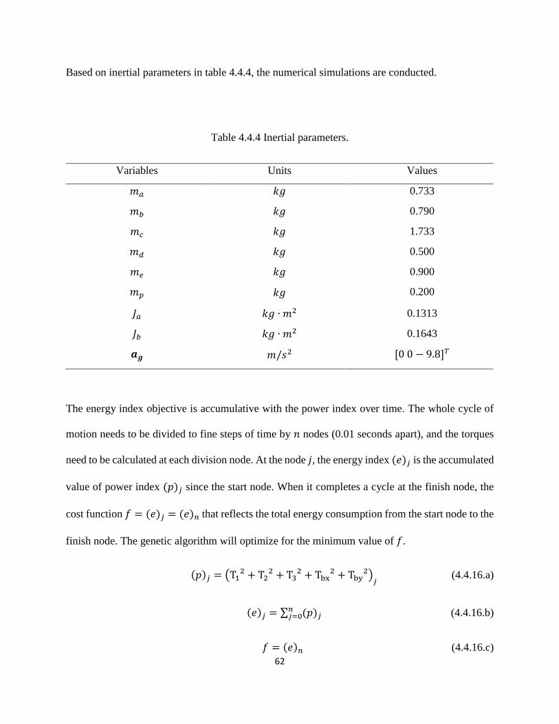
62

Based on inertial parameters in table 4.4.4, the numerical simulations are conducted.

Table 4.4.4 Inertial parameters.

Variables Units Values

𝑚𝑎 𝑘𝑔 0.733

𝑚𝑏 𝑘𝑔 0.790

𝑚𝑐 𝑘𝑔 1.733

𝑚𝑑 𝑘𝑔 0.500

𝑚𝑒 𝑘𝑔 0.900

𝑚𝑝 𝑘𝑔 0.200

𝐽𝑎 𝑘𝑔 ∙ 𝑚2 0.1313

𝐽𝑏 𝑘𝑔 ∙ 𝑚2 0.1643

𝒂𝒈 𝑚/𝑠2 [0 0 − 9.8]𝑇

The energy index objective is accumulative with the power index over time. The whole cycle of

motion needs to be divided to fine steps of time by 𝑛 nodes (0.01 seconds apart), and the torques

need to be calculated at each division node. At the node 𝑗, the energy index (𝑒)𝑗 is the accumulated

value of power index (𝑝)𝑗 since the start node. When it completes a cycle at the finish node, the

cost function 𝑓 = (𝑒)𝑗 = (𝑒)𝑛 that reflects the total energy consumption from the start node to the

finish node. The genetic algorithm will optimize for the minimum value of 𝑓.

(𝑝)𝑗 = (T12 + T2

2 + T32 + Tbx

2 + Tby2)

𝑗 (4.4.16.a)

(𝑒)𝑗 = ∑ (𝑝)𝑗𝑛𝑗=0 (4.4.16.b)

𝑓 = (𝑒)𝑛 (4.4.16.c)

63

Three runs are defined according to constraints. Among the three runs, run 1 takes all default

values, allowing neither relocation of joints nor motion planning of trajectory; run 2 allows joint

relocation alone but no motion planning; run 3 allows joint relocation plus motion planning. In

table 4.4.5, optimization results of variables 𝑥1~𝑥12, and the corresponding cost function 𝑓 are

given for run 1~3.

Table 4.4.5 Simulation results.

Run 𝑥1 𝑥2 𝑥3 𝑥4 𝑥5 𝑥6 𝑥7

1 1.394 1.394 1.394 -0.0732 0.2492 0.1221 -0.2808

2 1.511 1.196 1.21 -0.0732 0.2492 0.1221 -0.2808

3 1.515 1.173 1.216 0.025 0.237 0.056 -0.217

Run 𝑥8 𝑥9 𝑥10 𝑥11 𝑥12 𝑓

1 -0.6051 0.1221 0.6083 0.7937 0.5778 1110.1

2 -0.6051 0.1221 0.6083 0.7937 0.5778 1010.8

3 -0.525 0.166 0.62 0.788 0.574 908.22

64

Figure 4.4.4 The displacement of 𝜃𝑒𝑥, solid: original; dash: modified.

Figure 4.4.5 The displacement of 𝜃𝑒𝑦, solid: original; dash: modified.

65

Figure 4.4.6 The displacement of 𝑧𝑒, solid: original; dash: modified.

Figure 4.4.7 Energy index (𝑒)𝑗 increases over time, run 1, run 2, run 3.

66

Table 4.4.6 Trajectory function factors.

Run 𝑎12 𝑎11 𝑎10 𝑎9 𝑎8 𝑎7

1 𝜃𝑒𝑥(𝑡) 0 -0.0003 0.0047 -0.0398 0.2161 -0.8180

𝜃𝑒𝑦(𝑡) 0 0 0 -0.0001 0.0023 -0.0223

𝑧𝑒(𝑡) 0 0 0 -0.0001 0.0008 -0.0034

2 𝜃𝑒𝑥(𝑡) 0 -0.0003 0.0047 -0.0398 0.2161 -0.8180

𝜃𝑒𝑦(𝑡) 0 0 0 -0.0001 0.0023 -0.0223

𝑧𝑒(𝑡) 0 0 0 -0.0001 0.0008 -0.0034

3 𝜃𝑒𝑥(𝑡) 0 0 -0.0008 0.0160 -0.134 0.6020

𝜃𝑒𝑦(𝑡) 0 -0.0006 0.0085 -0.0733 0.3888 -1.3027

𝑧𝑒(𝑡) 0 0.0001 -0.0017 0.01563 -0.0901 0.3367

Run 𝑎6 𝑎5 𝑎4 𝑎3 𝑎2 𝑎1 𝑎0

1 𝜃𝑒𝑥(𝑡) 2.2409 -4.2723 4.8451 -2.2496 0 0 0

𝜃𝑒𝑦(𝑡) 0.1282 -0.4440 0.9003 -0.8451 0 0 0

𝑧𝑒(𝑡) 0.0033 0.0411 -0.1847 0.2513 0 0 0.5

2 𝜃𝑒𝑥(𝑡) 2.2409 -4.2723 4.8451 -2.2496 0 0 0

𝜃𝑒𝑦(𝑡) 0.1282 -0.4440 0.9003 -0.8451 0 0 0

𝑧𝑒(𝑡) 0.0033 0.0411 -0.1847 0.2513 0 0 0.5

3 𝜃𝑒𝑥(𝑡) -1.4876 1.8284 -0.7968 -0.00248 0 0 0

𝜃𝑒𝑦(𝑡) 2.7363 -3.4804 2.5779 -1.0716 0 0 0

𝑧𝑒(𝑡) -0.8202 1.2826 -1.2416 0.6385 0 0 0.5

The values of 𝑥4~𝑥12 in table 4.4.5 will be interpreted to the displacement/velocity/acceleration

polynomial functions for run1~3 in table 4.4.6. The results are plotted in figure 4.4.4 ~ figure 4.4.7.

Run 3 saves more energy than run 2, while run 1 takes highest energy consumption.

67

4.4.5 Theory Verification

The dynamic model of the 3-RRS is a group of rigid bodies that are connected by mechanical

joints. These elements have been established as editable blocks in Simulink library. The Simulink

simulation verifies the dynamic model based on classical Newton second law. The Simulink model

in linked blocks (figure 4.4.8) practices a sample task to validate the driving torques and dynamic

balancing. The modeled structure in 3D and its calculated dynamic motion could be viewed from

the visualization window (figure 4.4.9). So that one could check that the model is correctly built.

The inputs to the joint actuators are the required angular motions of joint 𝑩𝒊 of run1. The reaction

torques −𝑇𝑖 are measured from sensors which match the theoretical calculation (figure 4.4.10).

Furthermore, the reaction forces on base are measured at the 𝑩𝒊 joints which are equivalent to the

gravity of the manipulator (figure 4.4.11). The shaking forces is eliminated.

The dynamic simulation for a group of jointed rigid bodies is a common and mature function in

Simulink, of which the results can be trusted. The theoretical results and simulated results also

mutually prove each other. The experiments of real prototype may have errors due to

manufacturing/control defects thus is not recommended, while the Simulink could build an ideal

model for theory verification.

68

Figure 4.4.8 The Simulink model of the manipulator in blocks.

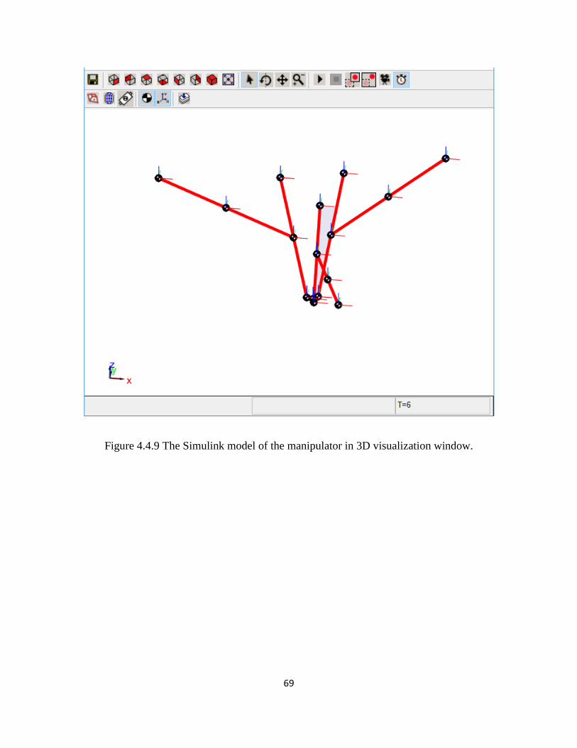
69

Figure 4.4.9 The Simulink model of the manipulator in 3D visualization window.

70

Figure 4.4.10 The reaction torques −𝑇1, −𝑇2 and −𝑇3 sensor value and theoretical value.

71

Figure 4.4.11 The base reaction forces along 𝒙𝐨, 𝒚𝐨 and 𝒛𝐨 axes.

72


A balanced 3-RRS parallel manipulator is designed with passive force balancing and active

moment balancing. Joints relocation and trajectory planning are the adaption that provides solution

to energy saving while the task requirements of the motion are satisfied. When more variables are

involved, the better optimization results would be obtained. The structural adaption plus motion

planning yields the best optimization effect. The dynamic model is verified by Simulink

simulation. In automated manufacturing industry that largely rely on parallel robotic manipulators,

the adaption promotes environment-friendly green operations as large amount of energy can be

saved in repeated cyclic motions on production lines. The energy saving impact would be

remarkable when this design and its method are implemented on large scale.

4.5 Combination for High DOF Mechanism

Fully parallel robots of high-DOF have more limbs that restrict the workspace. Balancer or limb

interference avoidance is more complex. Serial type hybrid robots have larger workspace but the

increased load on platform greatly increase the counter mass on the parallel limbs which could

take more energy. The design is a challenge. Structure adaption is even more challenging.

The (2-RR)R and 3-RRS are interference free and structural adaptive. They could be combined.

The combined manipulator is interference free. The DOF is combined and the structural adaption

is also combined.

73

When the (2-RR)R planar manipulator adds one more motor at the end effector, this manipulator

will have 3 DOFs that are two translations and one rotation on a plane. The combined (2-RR)R

and 3-RRS will have 6 DOF in total.

There are merits of the combined manipulator compared to an individual manipulator with same

DOFs. It uses a separate planar manipulator, the (2-RR)R, for planar motions instead of having to

move the 3-RRS. therefore it is simpler and lighter. It requires less actuation energy as the actuation

is distributed to two manipulators.

This application of the design could be in manufacturing where one manipulator holds a work

piece and the other manipulator is working on it.

74

Figure 4.5.1 The combination of balanced robots.


This chapter discusses the interference-free design for dynamically balanced manipulators and

their energy consumption optimization. The passive force balancing and active moment balancing

are integrated for a planar (2-RR)R robot and a spatial 3-RRS robot dynamic balancing solution.

The configurations are changed through middle revolute joint angle reversal to avoid link

75

interference. The structure adaption and motion planning are conducted for optimal energy

purposes. As is seen from the planar (2-RR)R operations, the structural adaption could reduce

energy consumption for a certain trajectory and the optimization effect depends on the trajectory.

As is seen from the spatial 3-RRS operations, the structural adaption alone could save energy while

the integration of structural adaption and motion planning could save more energy. The inclusion

of more variables could result to better optimization effect. The dynamic model of the spatially

balanced 3-RRS manipulator obtained by D’Alembert’s principle is verified by Simulink.

The planar 2-DOF (2-RR)R robot can be modified to become a planar 3-DOF (2-RR)R robot which

is to be combined with 3-RRS to make a 6-DOF balanced robot interference-free. Structural

adaptions are also combined from two manipulators which simplifies the complexity of structure.

The five joints with adaptive relocation in the combined machine conveniently offer many

opportunities for optimization. The actuation loads are distributed to two manipulators which make

the combined 6-DOF manipulator lighter, simpler and energy saving.

76

Chapter 5 Deployable 3-DOF P*U* Parallel Manipulators


This chapter discusses the re-design of 3-DOF P*U* parallel manipulators with adaptive features

for optimization. The applications of the designs are in solar tracking.

As the sun rises in the east, sets in the west and inclination angle changes with seasons, the solar

trackers are designed to follow the sun. There are some designs of solar trackers. A 1-DOF solar

tracker is designed with one rotation [144]. Serial robots of 2-DOF [145] [146] so that the tracker

could rotate from east to west and from north to south. The solar panel is heavy. As the parallel

robots have advantages in precision and loading, some solar trackers are designed with parallel

manipulator as the stand. A parallel solar tracker is designed with 2-DOF [147] for the two rotation

angles. A parallel tracker is designed with 2R1T 3-PRS [148] so it has one more vertical

translational motion in addition to the two rotations. Another 2R1T parallel structure is designed

with 3-RPS [149]. The parallel tracker which could provide two rotations and one vertical

translation has one more degree of freedom. It provides convenience for repair and maintenance,

while some performance such as stiffness or actuation could be optimized through adjustable

height of the platform.

Although one could find plenty of solar tracker designs, the deployable re-design of the solar

trackers and relevant researches are rare.

The solar panel is a large surface. Wind loads on panel needs to be considered. As suggested in

researches [150] and [151], the wind loads could be divided to a lift force and a drag force, where

77

the lift force is normal to the panel and the drag force is parallel to the panel. Storm hazards are

frequent in tropical Asia Pacific regions [119]. In North America, the news report of solar field

destroyed by storm or tips of storm protection [120] [121] are heard.

Wind is a destructive power but also a clean source of energy. Piezo materials could convert

mechanical motion or deformation to electric energy [152]. Piezo chips are used in several designs

to collect energy from wind loads [153] [154] [155]. Besides wind energy, some structure is

designed to harvest energy from mechanical motion. A 6-DOF parallel structure is designed which

is not actuated by motors but passively receive vibration for energy harvesting [156].

Parallel solar trackers could be designed to harvest energy from wind loads on the large solar panel

which makes them hybrid energy harvesters. The parallel manipulators have higher stiffness and

loads capacity suitable for working in the winds and can be re-designed with deployable function

that allows them to lie down for storm protection. Adaption is considered and added to the original

structure for optimization.

The minimum deployable height could be determined after evaluation of loading capacity and

other constraints.

An adjustable 3-PRS solar tracking stand is designed to show the concept of deployable solar

tracker with lie-flat function. The larger workspace and higher general stiffness are the outcome

of multi-objective optimization through structural adaption.

Another adjustable 3-RPS hybrid energy harvester is designed considering the operational

requirements of dust proof and real models of actuation products are selected for the design.

Minimum height algorithm and Jacobian transformation are developed to assist the evaluation of

the design. Piezo chips are included for wind energy harvesting.

78


The design needs to provide a folded pose considering the loading capacity and the retracted length

of the actuators. A lie-flat vectors diagram is given in the design of 3-RPS parallel manipulator

which determines the height of the platform at lie-flat pose.

Minimum platform height algorithm is the intersection of qualified solutions for constraints. This

algorithm could rapidly calculate the eligible orientations of the platform due to the nature of solar

tracking functions.

Jacobian matrix is modified to analyse the stiffness in directions other than the cartesian global

coordinate axes. This assists the stiffness evaluation in practical situation where the wind loads

may be horizontal in any direction.

The 3-PRS and 3-RPS are designed with adjustable base joint locations for optimization. Paper

[78] discussed a 3-PRS robot which changes between different operational modes through the rail

angle adjustments. The angles or locations of the base joints could indicate a specific operational

mode the manipulator is in. The working and lie-flat are two operational modes of solar trackers

as well.

5.3 Adaptive 3-PRS Parallel Manipulator

The solar tracking stand adjusts its pose timely to have the solar panel properly face to the moving

sun. A 3-PRS parallel manipulator is designed that provides high stiffness and easy maintenance.

The structural adaption of the 3-PRS parallel stand allows further optimization of workspace and

79

stiffness with respect to seasons. The research discusses an optimized design for green energy

collection.

5.3.1 The 3-PRS Mechanism Design

The solar tracking stand needs to be designed satisfying large workspace, high stiffness, and easy

maintenance. The parallel legs of the stand share the load of the panel, and reduce the deformation

thus taking the advantage of higher stiffness. Besides the advantage in stiffness, it should facilitate

maintenance. The design should be able to reach a pose to avoid storm damage. This design can

keep the solar panel flat and in a very low position when destructive weather occurs.

The non-adaptive 3-PRS stand (figure 5.3.1 (a)) with flat base rails on the ground can fold its legs

and stay low, close to the ground when strong storms hit so as to protect the structure from the

powerful blow on its panel face (figure 5.3.1 (b)). And the motion of the platform in vertical way

helps to adjust the height for convenience in panel maintenance and repair. The concept of adaptive

can be considered to have the prismatic rails adjustable in the inclination angle to the ground

(figure 5.3.1 (c)). The main benefit of the structure adaption is that it adds more parameters to be

tuned in favor of the operation conditions, while it can still reach the storm protection pose (figure

5.3.1 (d)).

The adaptive 3-PRS is the design to be discussed in this section. The adjustable prismatic rails can

set the inclination angles. The slider moves along the rail, and is attached to the bottom of the leg

with a revolute joint. At the top of the leg, it is attached to the platform each with a spherical joint.

There are three identical sets of adaptive rails and legs, each can be adjusted individually. The

structure can be written in full as 3-PR*PRS.

80

Figure 5.3.1 The 3-PRS parallel stand. (a) non-adaptive 3-PRS design; (b) storm protection pose

for non-adaptive design; (c) adaptive 3-PRS design; (d) storm protection pose for adaptive

design.

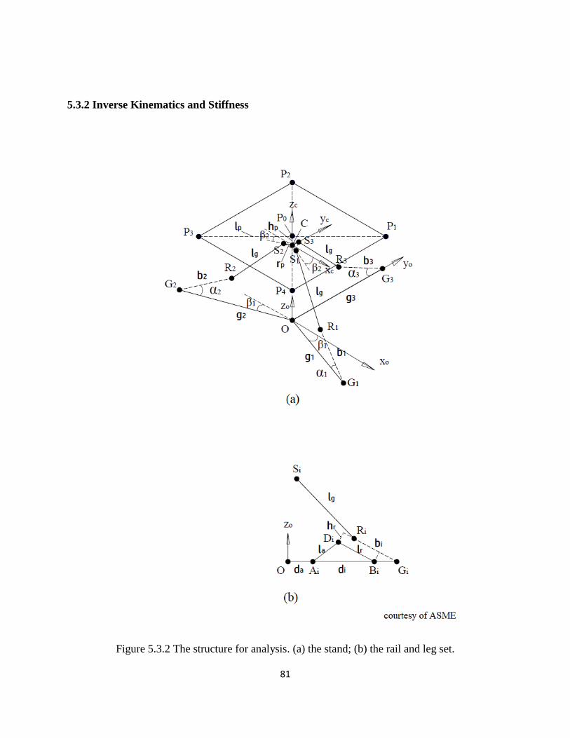
81

5.3.2 Inverse Kinematics and Stiffness

Figure 5.3.2 The structure for analysis. (a) the stand; (b) the rail and leg set.

82

As is shown in figure 5.3.2, a square solar panel is mounted on the top of the stand with four

vertices 𝑷𝒊 at a distance of 𝑙𝑝 from the panel center at 𝑷𝟎. A moving coordinate 𝑥𝑐𝑦𝑐𝑧𝑐 is set at

point 𝑪 which is the center of the platform attached to the three spherical joints, and it is under the

solar panel center 𝑷𝟎 by distance ℎp. The spherical joints are represented with points 𝑺𝒊, and the

revolute joints at the end of the leg are 𝑹𝒊. The length of the leg 𝑙𝑔 is measured from the spherical

joint to the revolute joint. The slider attached to these revolute joints slide along the rails parallel

to rail bottom line 𝑫𝒊𝑩𝒊, which connects revolute joints at 𝑫𝒊 and 𝑩𝒊. The revolute joint 𝑹𝒊

measures a distance ℎ𝑟 from 𝑫𝒊𝑩𝒊. There is a revolute joint 𝑨𝒊 on each base guideway. The

distance 𝑑𝑖 is adjusted to adjust the rail inclination angle 𝛼𝑖. A line parallel to 𝑫𝒊𝑩𝒊 passing

revolute joint 𝑹𝒊 intersect the ground at point 𝑮𝒊, which is an imaginary point. A fixed coordinate

𝑥𝑜𝑦𝑜𝑧𝑜 is at the point 𝑶 where the three ground guide ways meet.

The coordinate axes are given below.

𝒙𝒐 = [1 0 0]𝑇, 𝒚𝒐 = [0 1 0]𝑇, 𝒛𝒐 = [0 0 1]𝑇 (5.3.1)

The rail inclination angle is adjusted as the equation explains.

𝛼𝑖 = 𝑐𝑜𝑠−1(𝑙𝑟

2+𝑑𝑖2−𝑙𝑎

2

2𝑙𝑟𝑑𝑖) (5.3.2.a)

and it is adjusted through sliders on the base guideways.

𝑔𝑖 = 𝑑𝑎 + 𝑑𝑖 +ℎ𝑟

𝑠𝑖𝑛𝛼𝑖 (5.3.2.b)

83

Inverse Kinematic method is used to solve for the actuator positions based on the given end effector

positions. The orientation of the platform is 𝑹𝒙𝒚. The positions of the spherical joints are

calculated.

𝑺𝒊 = 𝑹𝒙𝒚𝑺 + 𝑪 (5.3.3.a)

where

𝑹𝒙𝒚 = [

𝑐𝑜𝑠𝜃𝑦 0 𝑠𝑖𝑛𝜃𝑦

𝑠𝑖𝑛𝜃𝑥𝑠𝑖𝑛𝜃𝑦 𝑐𝑜𝑠𝜃𝑥 −𝑠𝑖𝑛𝜃𝑥𝑐𝑜𝑠𝜃𝑦

−𝑐𝑜𝑠𝜃𝑥𝑠𝑖𝑛𝜃𝑦 𝑠𝑖𝑛𝜃𝑥 𝑐𝑜𝑠𝜃𝑥𝑐𝑜𝑠𝜃𝑦

] (5.3.3.b)

and the spherical joints positions with reference to the platform center are expressed as below,

𝑺 = [𝑟𝑝 cos 𝛽𝐺𝑖 𝑟𝑝 sin 𝛽𝐺𝑖 0]𝑇 (5.3.3.c)

Where

𝛽𝐺1 = −𝛽1, 𝛽𝐺2 = 𝜋 + 𝛽2, 𝛽𝐺3 =𝜋

2 (5.3.3.d)

and the center of the moving platform, center of the spherical joints, is positioned as below.

𝑪 = [𝑥𝑐 𝑦𝑐 𝑧𝑐]𝑇 (5.3.3.e)

The three coordinates of 𝑺𝒊 is given below.

𝑺𝒊 = [𝑠𝑖𝑥 𝑠𝑖𝑦 𝑠𝑖𝑧]𝑇 (5.3.3.f)

The 𝑺𝒊 points are in three vertical planes.

𝑠3𝑥 = 0 and 𝑠2𝑦 = 𝑠2𝑥tan 𝛽𝑠2 (5.3.3.g)

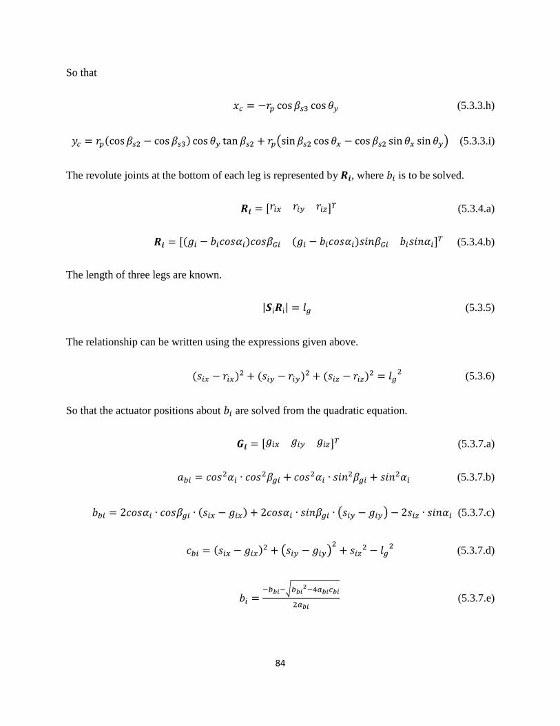
84

So that

𝑥𝑐 = −𝑟𝑝 cos 𝛽𝑠3 cos 𝜃𝑦 (5.3.3.h)

𝑦𝑐 = 𝑟𝑝(cos𝛽𝑠2 − cos 𝛽𝑠3) cos 𝜃𝑦 tan 𝛽𝑠2 + 𝑟𝑝(sin 𝛽𝑠2 cos 𝜃𝑥 − cos 𝛽𝑠2 sin 𝜃𝑥 sin 𝜃𝑦) (5.3.3.i)

The revolute joints at the bottom of each leg is represented by 𝑹𝒊, where 𝑏𝑖 is to be solved.

𝑹𝒊 = [𝑟𝑖𝑥 𝑟𝑖𝑦 𝑟𝑖𝑧]𝑇 (5.3.4.a)

𝑹𝒊 = [(𝑔𝑖 − 𝑏𝑖𝑐𝑜𝑠𝛼𝑖)𝑐𝑜𝑠𝛽𝐺𝑖 (𝑔𝑖 − 𝑏𝑖𝑐𝑜𝑠𝛼𝑖)𝑠𝑖𝑛𝛽𝐺𝑖 𝑏𝑖𝑠𝑖𝑛𝛼𝑖]𝑇 (5.3.4.b)

The length of three legs are known.

|𝑺i𝑹i| = 𝑙𝑔 (5.3.5)

The relationship can be written using the expressions given above.

(𝑠𝑖𝑥 − 𝑟𝑖𝑥)2 + (𝑠𝑖𝑦 − 𝑟𝑖𝑦)2 + (𝑠𝑖𝑧 − 𝑟𝑖𝑧)

2 = 𝑙𝑔2 (5.3.6)

So that the actuator positions about 𝑏𝑖 are solved from the quadratic equation.

𝑮𝒊 = [𝑔𝑖𝑥 𝑔𝑖𝑦 𝑔𝑖𝑧]𝑇 (5.3.7.a)

𝑎𝑏𝑖 = 𝑐𝑜𝑠2𝛼𝑖 ∙ 𝑐𝑜𝑠2𝛽𝑔𝑖 + 𝑐𝑜𝑠2𝛼𝑖 ∙ 𝑠𝑖𝑛2𝛽𝑔𝑖 + 𝑠𝑖𝑛2𝛼𝑖 (5.3.7.b)

𝑏𝑏𝑖 = 2𝑐𝑜𝑠𝛼𝑖 ∙ 𝑐𝑜𝑠𝛽𝑔𝑖 ∙ (𝑠𝑖𝑥 − 𝑔𝑖𝑥) + 2𝑐𝑜𝑠𝛼𝑖 ∙ 𝑠𝑖𝑛𝛽𝑔𝑖 ∙ (𝑠𝑖𝑦 − 𝑔𝑖𝑦) − 2𝑠𝑖𝑧 ∙ 𝑠𝑖𝑛𝛼𝑖 (5.3.7.c)

𝑐𝑏𝑖 = (𝑠𝑖𝑥 − 𝑔𝑖𝑥)2 + (𝑠𝑖𝑦 − 𝑔𝑖𝑦)

2+ 𝑠𝑖𝑧

2 − 𝑙𝑔2 (5.3.7.d)

𝑏𝑖 =−𝑏𝑏𝑖−√𝑏𝑏𝑖

2−4𝑎𝑏𝑖𝑐𝑏𝑖

2𝑎𝑏𝑖 (5.3.7.e)

85

The actuator displacements are solved, but there are poses that need to be avoided, so that criteria

need to be set for eligibility of poses. Only the solutions that make sense can be considered as

valid.

Criteria 1. The edge of the platform should be above ground. So all the vertices are above the

ground.

(𝑷𝒋)𝑧> 0, 𝑗 = 1,2,3,4 (5.3.8.a)

Criteria 2. The leg should be above the rail, and the leg with rail should be under the platform.

For the leg to be above the inclined rails, the following criteria need to be met.

𝒏𝒐 = [0 0 1]𝑇 (5.3.8.b)

𝑑𝑝𝑔𝑖 = ((𝒏𝒐 × 𝑶𝑮i) × 𝑮i𝑹i) ∙ 𝑹i𝑺i > 0 (5.3.8.c)

For the leg and rail to be under the platform surface, the following criteria should be met.

𝒏𝒄 = 𝑷𝟏𝑷𝟐 × 𝑷𝟐𝑷𝟑 (5.3.9.a)

𝑷𝒐 =(𝑷𝟏+𝑷𝟑)

2 (5.3.9.b)

𝑑𝑝𝑠𝑖 = 𝑷𝟎𝑮i ∙ 𝒏𝒄 < 0 (5.3.9.c)

Criteria 3. The actuator displacements 𝑏𝑖 need to be real positive values. And the slider needs to

stay on the rail.

(𝑏𝑖 −ℎ𝑟

𝑡𝑎𝑛𝛼𝑖) ∈ [𝑟𝑚𝑖𝑛, 𝑟𝑚𝑎𝑥] (5.3.10)

86

The Jacobian matrix represents the relationship between velocities of actuators and end effector.

An algebraic method for solution to 3-PRS manipulator can be found in [14].

The relationship of the constant leg length is utilized to obtain the matrix.

𝑒𝑖 = (𝑠𝑖𝑥 − 𝑟𝑖𝑥)2 + (𝑠𝑖𝑦 − 𝑟𝑖𝑦)2 + (𝑠𝑖𝑧 − 𝑟𝑖𝑧)

2 − 𝑙𝑔2 (5.3.11.a)

So that,

𝑒𝑖 = (cot2 𝛽𝐺𝑖 + 1) ∙ (𝑠𝑖𝑦 − 𝑟𝑖𝑦)2 + (𝑠𝑖𝑧 − 𝑟𝑖𝑧)2 − 𝑙𝑔

2 (5.3.11.b)

First, the actuator displacement about spherical joint is found. (This equation below is modified

from the one in [28] to reflect the mutual relationship between 𝛿𝑠𝑖𝑥 and 𝛿𝑠𝑖𝑦.)

(𝜕𝑒𝑖

𝜕𝑏𝑖) 𝛿𝑏𝑖 = [

𝜕𝑒𝑖

𝜕𝑠𝑖𝑦

𝜕𝑒𝑖

𝜕𝑠𝑖𝑧] ∙ [𝛿𝑠𝑖𝑦 𝛿𝑠𝑖𝑧]𝑇 (5.3.11.c)

Then the motion of actuators is related to the end effector.

[𝛿𝑠𝑖𝑦 𝛿𝑠𝑖𝑧]𝑇 = [𝐽𝑖][𝛿𝜃𝑥 𝛿𝜃𝑦 𝛿𝑧𝑐]𝑇 (5.3.12.a)

where,

[𝐽𝑖] = [

𝜕𝑠𝑖𝑦

𝜕𝜃𝑥

𝜕𝑠𝑖𝑦

𝜕𝜃𝑦

𝜕𝑠𝑖𝑦

𝜕𝑧𝑐

𝜕𝑠𝑖𝑧

𝜕𝜃𝑥

𝜕𝑠𝑖𝑧

𝜕𝜃𝑦

𝜕𝑠𝑖𝑧

𝜕𝑧𝑐

] (5.3.12.b)

So that, the actuator displacement is solved. This is expressed in an equation about the end effector.

𝛿𝑏𝑖 = [𝜕𝑒𝑖

𝜕𝑠𝑖𝑦/

𝜕𝑒𝑖

𝜕𝑏𝑖

𝜕𝑒𝑖

𝜕𝑠𝑖𝑧/

𝜕𝑒𝑖

𝜕𝑏𝑖] [𝐽𝑖][𝛿𝜃𝑥 𝛿𝜃𝑦 𝛿𝑧𝑐]𝑇 (5.3.13)

The Jacobian matrix is built from the above equations.

87

𝐽 =

[ [

𝜕𝑒1

𝜕𝑠1𝑦/

𝜕𝑒1

𝜕𝑏1

𝜕𝑒1

𝜕𝑠1𝑧/

𝜕𝑒1

𝜕𝑏1] [𝐽1]

[𝜕𝑒2

𝜕𝑠2𝑦/

𝜕𝑒2

𝜕𝑏2

𝜕𝑒2

𝜕𝑠2𝑧/

𝜕𝑒2

𝜕𝑏2] [𝐽2]

[𝜕𝑒3

𝜕𝑠3𝑦/

𝜕𝑒3

𝜕𝑏3

𝜕𝑒3

𝜕𝑠3𝑧/

𝜕𝑒3

𝜕𝑏3] [𝐽3]]

(5.3.14.a)

where

𝜕𝑒𝑖

𝜕𝑠𝑖𝑦= 2(cot2 𝛽𝐺𝑖 + 1)(𝑠𝑖𝑦 − 𝑟𝑖𝑦) (5.3.14.b)

𝜕𝑒𝑖

𝜕𝑠𝑖𝑧= 2(𝑠𝑖𝑧 − 𝑟𝑖𝑧) (5.3.14.c)

and

𝜕𝑒𝑖

𝜕𝑏𝑖= 2𝑏𝑖 − 2𝑠𝑖𝑧𝑠𝑖𝑛𝛼𝑖 + 2𝑐𝑜𝑠𝛼𝑖[𝑐𝑜𝑠𝛽𝑔𝑖(𝑠𝑖𝑥 − 𝑔𝑖𝑐𝑜𝑠𝛽𝑔𝑖) + 𝑠𝑖𝑛𝛽𝑔𝑖(𝑠𝑖𝑦 − 𝑔𝑖𝑠𝑖𝑛𝛽𝑔𝑖)] (5.3.14.d)

The end effector stiffness 𝑲 is calculated with the actuation stiffness 𝑲𝑱.

𝑲 = 𝑱𝑻𝑲𝑱𝑱 (5.3.15)

The general stiffness (global stiffness) the summation of the diagonal elements of matrix, judges

the overall stiffness performance of a mechanism and is to be optimized.

𝑔𝑠 = 𝑲(1,1) + 𝑲(2,2) + 𝑲(3,3) (5.3.16)

5.3.3 Adaption and Operation Optimization

The solar tracking stand is expected to have a large workspace to follow the motion of the sun and

it needs high stiffness to restrict deformation due to the wind blow. To maximize both workspace

and general stiffness of the parallel stand, the Pareto front can be used to find the optimized points.

88

Optimization with regards to the changing seasons can serve the objectives better than keeping the

same configuration for the whole year. This is a benefit of having adaptive solar tracking stand.

With Pareto front, it is capable to practice double objective optimization. In MATLAB, it seeks

minimum value. In order to seek maximum, the value is presented in minus. The two objectives

are given below.

𝑓1 = −𝑛 (5.3.17.a)

𝑓2 = −𝑙𝑛((∑ 𝑔𝑠𝑛𝑖=1 ) 𝑛⁄ ) (5.3.17.b)

where the first objective is to count eligible points in a given area by defined intervals so as to

measure the workspace, while the second objective is to calculate the natural logarithm of general

stiffness on average for all the points counted in the first objective. The two objectives serve as the

cost functions of the optimization.

The above two objectives are dependant on selected seasons. There is a pre-optimization before

this two-objective operation optimization. The pre-optimization guides the setting of design

parameters in table 5.3.1.

The workspace is defined as a coordinate with respect to 𝜃𝑥 and 𝜃𝑦 based on the installation

position that has x axis of the base align with the east-west and y axis align with north-south.

Suppose the required motions during each season are located in areas separated with boundaries

by the parabola (figure 5.3.3), the points within a given area represent the orientations needed for

the solar tracking in this season. This allows seasonal optimization for best workspace and general

stiffness. The parabola boundaries vary when latitude changes.

The parameters are in table 5.3.2.

89

Table 5.3.1 Design parameters of the adaptive stand.

Parameters Unit Values

𝛽𝑝𝑖 rad [𝜋

4,𝜋

2,3𝜋

4, 𝜋]

ℎ𝑝 m 0.05

𝛽1 rad 𝜋

6

𝛽2 rad 𝜋

6

𝑟𝑝 m 0.04

𝑙𝑔 m 0.4

𝑙𝑝 m 0.5

𝐾𝑎,𝑒,𝑛 N/m 100000

𝑑𝑎 m 0.08

ℎ𝑟 m 0.05

𝑙𝑎 m 0.16

𝑙𝑟 m 0.16

Parabola 0:

𝜃𝑥 = 𝑎0𝜃𝑦2 + 𝑐0 (5.3.18.a)

Parabola 1:

𝜃𝑥 = 𝑎1𝜃𝑦2 + 𝑐1 (5.3.18.b)

Parabola 2:

𝜃𝑥 = 𝑎2𝜃𝑦2 + 𝑐2 (5.3.18.c)

Parabola 3:

𝜃𝑥 = 𝑎3𝜃𝑦2 + 𝑐3 (5.3.18.d)

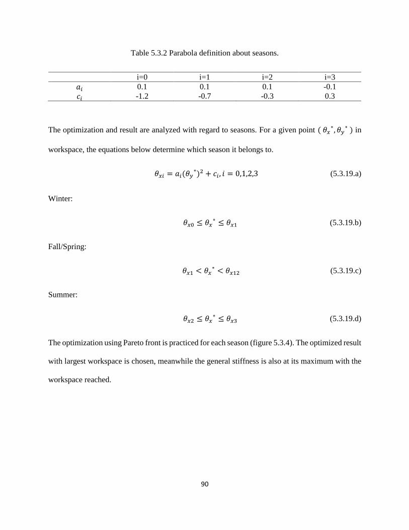
90

Table 5.3.2 Parabola definition about seasons.

i=0 i=1 i=2 i=3

𝑎𝑖 0.1 0.1 0.1 -0.1

𝑐𝑖 -1.2 -0.7 -0.3 0.3

The optimization and result are analyzed with regard to seasons. For a given point ( 𝜃𝑥∗, 𝜃𝑦

∗ ) in

workspace, the equations below determine which season it belongs to.

𝜃𝑥𝑖 = 𝑎𝑖(𝜃𝑦∗)2 + 𝑐𝑖 , 𝑖 = 0,1,2,3 (5.3.19.a)

Winter:

𝜃𝑥0 ≤ 𝜃𝑥∗ ≤ 𝜃𝑥1 (5.3.19.b)

Fall/Spring:

𝜃𝑥1 < 𝜃𝑥∗ < 𝜃𝑥12 (5.3.19.c)

Summer:

𝜃𝑥2 ≤ 𝜃𝑥∗ ≤ 𝜃𝑥3 (5.3.19.d)

The optimization using Pareto front is practiced for each season (figure 5.3.4). The optimized result

with largest workspace is chosen, meanwhile the general stiffness is also at its maximum with the

workspace reached.

91

Figure 5.3.3 Four parabola for seasonal division.

The table 5.3.3, 5.3.4 and 5.3.5 shows the adjustment of 𝑑1, 𝑑2, 𝑑3 and 𝑧𝑐, with optimized results

for each season respectively.

Table 5.3.3 Winter optimization.

Parameters Unit Range Values

𝑑1, 𝑑2 m [0.1,0.32] 0.167

𝑑3 m [0.1,0.32] 0.274

𝑧𝑐 m [0.3,0.7] 0.7

𝑓1 NA NA -119

𝑓2 NA NA -15.166

92

Table 5.3.4 Fall/Spring optimization.


𝑑1, 𝑑2 m [0.1,0.32] 0.147

𝑑3 m [0.1,0.32] 0.273

𝑧𝑐 m [0.3,0.7] 0.694

𝑓1 NA NA -97

𝑓2 NA NA -15.478

Table 5.3.5 Summer optimization.


𝑑1, 𝑑2 m [0.1,0.32] 0.173

𝑑3 m [0.1,0.32] 0.279

𝑧𝑐 m [0.3,0.7] 0.654

𝑓1 NA NA -116

𝑓2 NA NA -15.604

Seasonal adaption reaches an optimized result with largest workspace and the largest general

stiffness with this workspace. The eligible reachable workspace by the platform for each season,

and the general stiffness mapping over the workspace are given in figure 5.3.5.

93

Figure 5.3.4 Optimization using pareto front. (a) winter; (b) fall/spring; (c) summer.

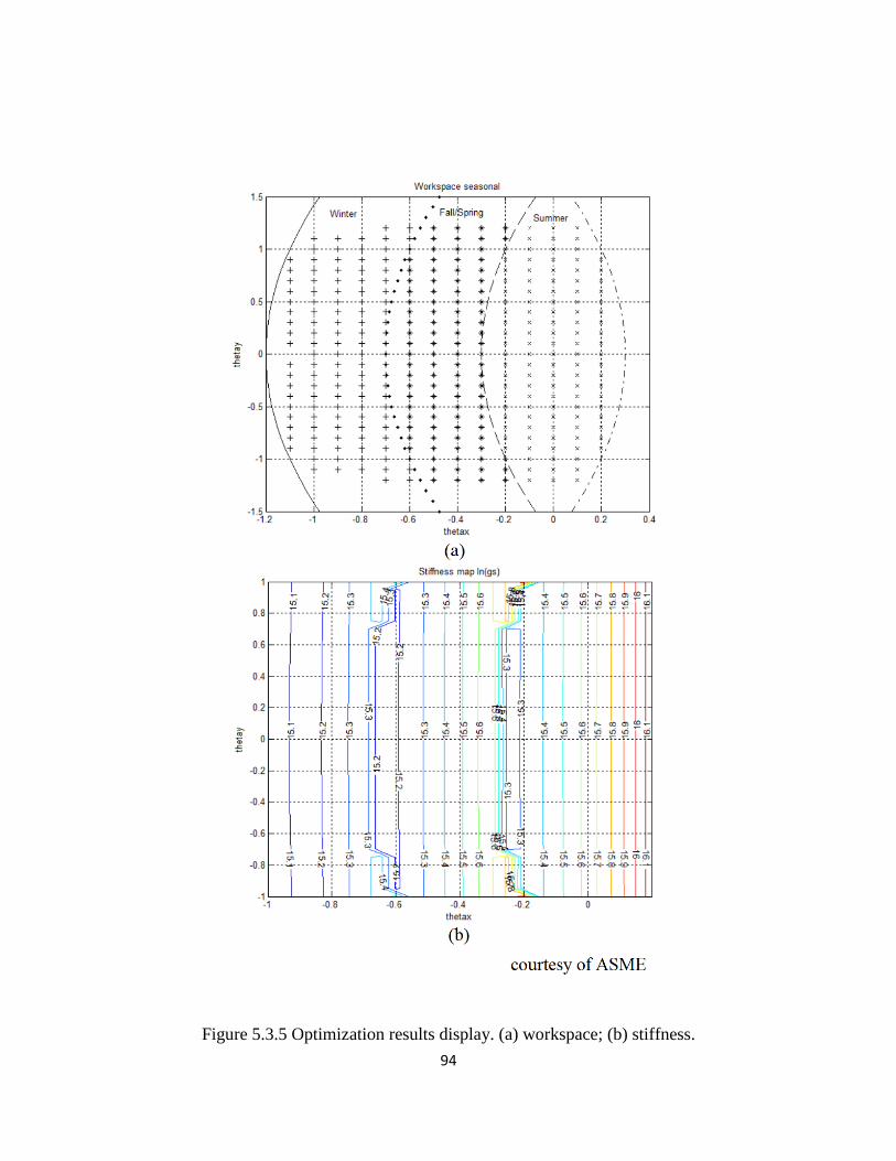
94

Figure 5.3.5 Optimization results display. (a) workspace; (b) stiffness.

95

In a same season, the centre of mass of platform is at constant height, so to keep the platform

height from being fluctuating to save the energy.


The solar tracking stand in parallel 3-PRS has a pre-optimization to the guide the setting of design

parameters, and a separate two-objective optimization that deals with operational objectives in

selected areas for workspace and general stiffness. This design has advantage of high general

stiffness and easy maintenance including a protection pose that allows it to lie flat on ground during

destructive storms. The parallel stand can be adjusted with regards to seasons. Best workspace and

stiffness are sought as season changes. Optimizing the objectives by season provides a better

performance than any fixed configuration. This is an important advantage of the adaptive solar

tracking stand, which contributes to solar energy collection, a source of clean and free energy.

This is a concept design. One needs to consider the displacement limits of real actuators, dust proof

requirements in the fields. The inclination rail has three jointed points thus it is subject to bending.

Next section will discuss adaptive 3-RPS design fulfilling these requirements.

5.4 Adaptive 3-RPS Parallel Manipulator

This section presents the robotic structure and analysis of a hybrid energy harvester designed in

the form of a structural adaptive 3-RPS parallel manipulator, which tracks and collects solar energy

as a main function and also harvests energy from wind loads on the large solar panel. The adaptive

96

design allows the harvester to lie flat on floor when destructive storms occur and then return to a

working configuration after the storms. The workspace of the manipulator is determined by a

minimum platform height algorithm that is developed to find all reachable positions that compose

the workspace and also bring bending at root to least. The stiffness mapping of the harvester is

significant in evaluating its capacity to take wind loads, which a transformation matrix is

developed to convert to polar horizontal stiffness at end effector that is crucial to the intelligent

control strategy in decision to enter lie-flat configuration.

5.4.1 The 3-RPS Mechanism Design

This tracking stand is a 3-RPS parallel manipulator with lie-flat and working configuration

features.

The orientation angle and height of the solar panel could be adjusted by three actuated legs which

are jointed to motor-driven adjustable bases. The structure can be written in full as 3-PRPS.

As to meet the dust-proof, load capacity and geometric requirements for out-door working

conditions, the linear tables (model: Alpha 15-B-155) [157] and the linear actuators (model: DLA-

12-40-311-200-IP65) [158] are selected to function as adjustable base locations and telescopic legs

respectively. The spherical joint with large motion range [135] and piezo-chips incorporated

parallel structures are considered. Figure 5.4.1 shows the design in two configurations.

97

Figure 5.4.1 The hybrid harvester. (a) lie-flat configuration; (b) working configuration.

98


The inverse kinematics solves for the actuation displacements from a given posture of the platform.

In figure 5.4.2, the plane A represents the floor and the plane B represents a parallel plane above

floor. The global coordinate system 𝐴𝑜 − 𝑋𝑜𝑌𝑜𝑍𝑜 is located at 𝑨𝒐 underneath 𝑩𝒐 by ℎ𝑏.

𝑿𝒐 = [1 0 0]𝑇; 𝒀𝒐 = [0 1 0]𝑇; 𝒁𝒐 = [0 0 1]𝑇 (5.4.1)

𝑨𝒐 = [0 0 0]𝑇; 𝑩𝒐 = 𝑨𝒐 + ℎ𝑏𝒁𝒐 (5.4.2)

Figure 5.4.2 Inverse kinematic parallel structure.

99

Three points 𝑩𝟏, 𝑩𝟐, and 𝑩𝟑 are located on plane B where revolute joints are. One can connect

lines 𝑩𝒐𝑩𝒊, and finds angle 𝛽i between 𝑿𝒐and 𝑩𝒐𝑩𝒊. The length of 𝑩𝒐𝑩𝒊 is 𝑏𝑖 which can be

adjusted by base joint relocation. Sub-coordinates 𝐵𝑖 − 𝑋𝑏𝑖𝑌𝑏𝑖𝑍𝑜 are established at 𝑩𝟏, 𝑩𝟐, and

𝑩𝟑.

𝑿𝒃𝒊 = 𝑸𝒊𝑿𝒐 ; 𝒀𝒃𝒊 = 𝑸𝒊𝒀𝒐; where 𝑸𝒊 = [cos𝛽𝑖 −sin 𝛽𝑖 0sin 𝛽𝑖 cos 𝛽𝑖 0

0 0 1

] 𝑖 = 1,2,3 (5.4.3)

The platform is a triangle with 𝑪𝒐 at the center, while points 𝑪𝟏, 𝑪𝟐, and 𝑪𝟑 are at the three vertices

of the triangle where spherical joints are. One can connect lines 𝑪𝒐𝑪𝒊, the length of 𝑪𝒐𝑪𝒊 is a fixed

value 𝑟𝑐. One can set a sub-coordinate 𝐶𝑜 − 𝑋𝑐𝑌𝑐𝑁𝑐 at 𝑪𝒐, where 𝒀𝒄 aligns with vector 𝑪𝒐𝑪𝟏, 𝑿𝒄

lies on the triangle plane, and 𝑵𝒄 be a unit vector normal to the platform. The angle 𝛽i is between

𝑿𝒄 and 𝑪𝒐𝑪𝒊.

A square solar panel is attached above the platform by ℎ𝑝 in 𝑵𝒄 direction. The four points 𝑷𝟏, 𝑷𝟐,

𝑷𝟑 and 𝑷𝟒 are at the four points of the solar panel square. One can connect lines 𝑷𝒐𝑷𝒋, which

forms an angle 𝛽𝑝𝑗 from 𝑿𝒄, and the length of the lines is a fixed value 𝑟𝑝.

The vectors 𝑪𝒐𝑪𝒊 and 𝑷𝒐𝑷𝒋 from the perspective of coordinate 𝐶𝑜 − 𝑋𝑐𝑌𝑐𝑁𝑐 are given below.

𝑹𝒄𝒊 = [𝑟𝑐 ∙ cos 𝛽𝑖 𝑟𝑐 ∙ sin 𝛽𝑖 0]𝑇 , 𝑖 = 1,2,3 (5.4.4.a)

𝑹𝒑𝒋 = [𝑟𝑝 ∙ cos 𝛽𝑝𝑗 𝑟𝑝 ∙ sin 𝛽𝑝𝑗 0]𝑇 , 𝑗 = 1,2,3,4 (5.4.4.b)

One can connect 𝑩𝒊𝑪𝒊 along which the prismatic joints are, the length of which is 𝑞𝑖 ∈

[𝑞𝑚𝑖𝑛, 𝑞𝑚𝑎𝑥], and a unit vector 𝑿𝒒𝒊 is set along 𝑩𝒊𝑪𝒊. Vector 𝑿𝒒𝒊 forms an angle 𝜃𝑏𝑖 above the

plane B. In order to make sure that linear actuators operate under the moving platform, an angular

100

constraint 𝛾𝑐𝑚 is set which is the minimum angle the vector 𝑿𝒒𝒊 can form to platform plane (𝐶𝑜 −

𝐶1𝐶2𝐶3).

Relocation of the 𝑩𝒊 along 𝑿𝒃𝒊 introduces an adjustment variable 𝑏𝑖−𝑎𝑑𝑗. When 𝑏𝑖−𝑎𝑑𝑗 = 0,

variable 𝑏𝑖 is determined to allow minimum height of platform at the lie-flat posture.

Figure 5.4.3 Lie-flat vectors diagram.

The lie-flat vector diagram is shown in figure 5.4.3. It determines the height of the lie-flat pose.

𝑩𝒊 = 𝑏𝑖𝑸𝒊𝑿𝒐 + 𝑩𝒐, where 𝑏𝑖 = 𝑞𝑚𝑖𝑛cos𝛾𝑐𝑚 + 𝑟𝑐 + 𝑏𝑖−𝑎𝑑𝑗 (5.4.5)

Rotational matrix needs platform rotation variables 𝜃𝑥 and 𝜃𝑦 around 𝑿𝒐 and 𝒀𝒐 to convert vectors

or matrix in 𝐶𝑜 − 𝑋𝑐𝑌𝑐𝑁𝑐 to that in 𝐵𝑜 − 𝑋𝑜𝑌𝑜𝑍𝑜.

𝑢𝑥 =𝜃𝑥

𝜃 and 𝑢𝑦 =

𝜃𝑦

𝜃 , where 𝜃 = √𝜃𝑥

2 + 𝜃𝑦2 (5.4.6.a)

101

𝑹 = [

c 𝜃 + 𝑢𝑥2(1 − c 𝜃) 𝑢𝑥𝑢𝑦(1 − c𝜃) 𝑢𝑦 s 𝜃

𝑢𝑥𝑢𝑦(1 − c 𝜃) c 𝜃 + 𝑢𝑦2(1 − c 𝜃) −𝑢𝑥 s 𝜃

−𝑢𝑦 s 𝜃 𝑢𝑥 s 𝜃 c 𝜃

] (5.4.6.b)

One can set 𝑪𝒐 = [𝑥𝑐 𝑦𝑐 𝑧𝑐]𝑇 as its position in global coordinate. As 𝑩𝒊 is a revolute joint, then

𝑩𝒐𝑪𝒊 is perpendicular to 𝒀𝒃𝒊, which is a relationship to find kinematic solutions for 𝑥𝑐 and 𝑦𝑐.

So that,

𝑪 = [𝒀𝒃𝟐 ∙ 𝑿𝒐 𝒀𝒃𝟐 ∙ 𝒀𝒐

𝒀𝒃𝟑 ∙ 𝑿𝒐 𝒀𝒃𝟑 ∙ 𝒀𝒐]−1

∙ [𝑹𝑹𝒄𝟐 ∙ 𝒀𝒃𝟐

𝑹𝑹𝒄𝟑 ∙ 𝒀𝒃𝟑] (5.4.7.a)

which satisfies,

(𝑹𝑹𝒄𝒊 + 𝑪𝒐) ∙ 𝒀𝒃𝒊 = 0 (5.4.7.b)

𝑥𝑐 = 𝑪 ∙ 𝑿𝒐; 𝑦𝑐 = 𝑪 ∙ 𝒀𝒐 (5.4.7.c)

The variable 𝑧𝑐 is usually given by the motion planner, however improper selection of this value

can result to invalid solution. In this section, an algorithm is explained that seeks the minimum

height of platform center 𝑪𝒐 , 𝑧𝑐, if an eligible solution exists. This algorithm avoids missing valid

solutions while keeping minimum solar panel height to mitigate the wind loads bending effects at

structure root.

The minimum height algorithm starts by setting the initial value 𝑧𝑐𝑜.

𝑪𝒐∗ = [𝑥𝑐 𝑦𝑐 𝑧𝑐𝑜]𝑇 , where 𝑧𝑐𝑜 = 0 (5.4.8.a)

𝑪𝒊∗ = 𝑹𝑹𝒄𝒊 + 𝑪𝒐

∗; 𝑷𝒐

∗ = ℎ𝑝𝑹𝒁𝒐 + 𝑪𝒐∗; 𝑷𝒋

∗ = 𝑹𝑹𝒑𝒋 + 𝑷𝒐∗ (5.4.8.b)

102

In figure 5.4.4, possible candidates of 𝑧𝑐 are calculated by determining an offset as a supplement

to 𝑧𝑐𝑜. The offsets are determined considering some criteria. Offset 1: none of 𝑷𝒋 point should

stay below plane B; Offset 2: an angular constraint 𝛾𝑐𝑚 is met which is the minimum angle the

leg can form to platform plane (𝐶𝑜 − 𝐶1𝐶2𝐶3) under this platform; Offset 3: none of 𝑞𝑖 should be

less than 𝑞𝑚𝑖𝑛.

Offset 1, 𝑑o1:

𝑑o1 = ℎ𝑏 − 𝑧𝑝𝑖−𝑚𝑖𝑛, where 𝑧𝑝𝑖−𝑚𝑖𝑛 = 𝑚𝑖𝑛 (𝑷𝒊 ∙ 𝒁𝒐) (5.4.9.a)

𝑧𝑐−𝑐𝑎𝑛1 = 𝑧𝑐𝑜 + 𝑑o1 (5.4.9.b)

Offset2, 𝑑o2:

A unit vector 𝑿𝒄𝒊 is along the intersection line of planes 𝐶𝑜 − 𝐶1𝐶2𝐶3 and 𝑋𝑏𝑖 − 𝐵𝑖 − 𝑍𝑜.

𝑿𝒄𝒊 =𝒀𝒃𝒊×𝑵𝒄

|𝒀𝒃𝒊×𝑵𝒄| , where 𝑵𝒄 = 𝑹𝒁𝒐 (5.4.10.a)

𝜃𝑐𝑖 is an acute angle between planes 𝐶𝑜 − 𝐶1𝐶2𝐶3 and 𝑋𝑏𝑖 − 𝐵𝑖 − 𝑍𝑜.

𝜃𝑐𝑖 = cos−1|𝑵𝒄 ∙ 𝒀𝒃𝒊| (5.4.10.b)

It is imagined that 𝑿𝒄𝒊 is rotated at 𝑪𝒊 with an acute angle 𝛾𝑐𝑖 about 𝒀𝒃𝒊 to be altered to a new unit

vector 𝑿𝜸𝒊 which forms an angle 𝛾𝑐𝑚 to the platform plane 𝐶𝑜 − 𝐶1𝐶2𝐶3 or to its projection on the

platform in 𝑵𝒄 direction. The arrowhead of 𝑿𝜸𝒊 falls on a plane (𝐶𝑜 − 𝐶1𝐶2𝐶3)′ that is parallel to

platform plane and 𝑿𝜸𝒊 is in plane 𝑋𝑏𝑖 − 𝐵𝑖 − 𝑍𝑜. The gap between planes (𝐶𝑜 − 𝐶1𝐶2𝐶3)′ and

103

𝐶𝑜 − 𝐶1𝐶2𝐶3 is certain, and the intersection lines they make on plane 𝑋𝑏𝑖 − 𝐵𝑖 − 𝑍𝑜 are parallel

and the gap between which can be determined with 𝜃𝑐𝑖.

𝑿𝜸𝒊 = 𝑸𝒊 [cos 𝛾𝑐𝑖 0 sin 𝛾𝑐𝑖

0 1 0− sin 𝛾𝑐𝑖 0 cos 𝛾𝑐𝑖

]𝑸𝒊−𝟏𝑿𝒄𝒊 , where 𝛾𝑐𝑖 = sin−1 sin𝛾𝑐𝑚

sin𝜃𝑐𝑖 (5.4.10.c)

If 𝑪𝒊𝑩𝒊 is along 𝑿𝜸𝒊, the length of 𝑪𝒊𝑩𝒊 for it to reach 𝑩𝒊 is 𝑞𝑖−𝛾𝑐𝑚.

With 𝑿𝜸𝒊, 𝑞𝑖−𝛾𝑐𝑚 and 𝑪𝒊

∗, one can find an imagined point 𝑩𝜸𝒊 whose global coordinate in 𝒁𝒐 is

𝑧𝑏𝑖−𝑐.

𝑧𝑏𝑖−𝑐 = (𝑞𝑖−𝛾𝑐𝑚𝑿𝒒𝒊 + 𝑪𝒊

∗) ∙ 𝒁𝒐, where 𝑞𝑖−𝛾𝑐𝑚=

(𝑩𝒊−𝑪𝒊∗)∙𝑿𝒃𝒊

𝑿𝜸𝒊∙𝑿𝒃𝒊 (5.4.10.d)

Three legs each has its 𝑩𝜸𝒊 height, 𝑧𝑏𝑖−𝑐, and the minimum among them is selected so that an offset

is calculated based on the lowest 𝑩𝜸𝒊, thus the other two legs will be satisfied with the offset lift.

𝑑o2 = ℎ𝑏 − 𝑧𝑏𝑖−𝑐−𝑚𝑖𝑛, where 𝑧𝑏𝑖−𝑐−𝑚𝑖𝑛 = min (𝑧𝑏𝑖−𝑐) (5.4.10.e)

𝑧𝑐−𝑐𝑎𝑛2 = 𝑧𝑐𝑜 + 𝑑o2 (5.4.10.f)

Offset 3, 𝑑o3:

With 𝑪𝒊∗ and 𝑞𝑚𝑖𝑛, one can find an imagined 𝑩𝒒𝒊 under 𝑩𝒊 which ensures the minimum length of

linear actuators be met in all legs. The global coordinate of 𝑩𝒒𝒊 in 𝒁𝒐 is 𝑧𝑏𝑖−𝑞.

𝑧𝑏𝑖−𝑞 = 𝑪𝒊∗ ∙ 𝒁𝒐 − √𝑞𝑚𝑖𝑛

2 − ((𝑩𝒊 − 𝑪𝒊∗) ∙ 𝑿𝒃𝒊)

2 (5.4.11.a)

104

Three legs each has its 𝑩𝒒𝒊 height, 𝑧𝑏𝑖−𝑞, and the minimum among them is selected so that an

offset is calculated based on the lowest 𝑩𝒒𝒊 and the other two legs will be satisfied with the offset

lift.

𝑑o3 = ℎ𝑏 − 𝑧𝑏𝑖−𝑞−𝑚𝑖𝑛, where 𝑧𝑏𝑖−𝑞−𝑚𝑖𝑛 = min (𝑧𝑏𝑖−𝑞) (5.4.11.b)

𝑧𝑐−𝑐𝑎𝑛3 = 𝑧𝑐𝑜 + 𝑑o3 (5.4.11.c)

There are three 𝑧𝑐 candidates, each is the minimum height requirement in its offset calculation that

means it may have room to be enlarged. The maximum of the candidates is selected so that the

other two offset requirements are included under it.

𝑧𝑐 = max(𝑧𝑐−𝑐𝑎𝑛k) , k = 1,23 (5.4.12)

Once 𝑧𝑐 is determined, the posture needs to be calculated again with updated values.

𝑪𝒐 = [𝑥𝑐 𝑦𝑐 𝑧𝑐]𝑇 (5.4.13.a)

𝑪𝒊 = 𝑹𝑹𝒄𝒊 + 𝑪𝒐; 𝑷𝒐 = ℎ𝑝𝑹𝒁𝒐 + 𝑪𝒐; 𝑷𝒋 = 𝑹𝑹𝒑𝒋 + 𝑷𝒐 (5.4.13.b)

The motion of linear actuations are calculated based on the above platform position.

𝒒𝒊 = |𝑩𝒊 − 𝑪𝒊| and 𝜃𝑏𝑖 = tan−1 (𝑪𝒊−𝑩𝒊)∙𝒁𝒐

(𝑩𝒊−𝑪𝒊)∙𝑿𝒃𝒊 (5.4.14)

The updated value of 𝑧𝑐 will need to be verified. The posture with updated 𝑧𝑐 need to meet a

criteria that none of the linear actuators 𝑞𝑖 extends 𝑞𝑚𝑎𝑥, fully extended size.

Within 𝑛𝑟 pairs of (𝜃𝑥, 𝜃𝑦), program loops calculate 𝑧𝑐 at each (𝜃𝑥, 𝜃𝑦) and then verify. The

number of eligible solutions 𝑛𝑒 is an index to evaluate the workspace.

105

Figure 5.4.4 Minimum platform height 𝑧𝑐.

The 3-RPS manipulator has 3 DOF, that means it has three independent motions, while the other

motions in space are compliant to the independent motions.

In the global coordinate, the linear and angular velocities system of the end effector, center of the

platform 𝑪𝒐, is given below.

𝑽𝒄𝒐 = [𝜕𝑥𝑐 𝜕𝑦𝑐 𝜕𝑧𝑐]𝑇 and 𝝎𝒄𝒐 = [𝜕𝜃𝑐𝑥 𝜕𝜃𝑐𝑦 𝜕𝜃𝑐𝑧]𝑇 (5.4.15)

Only three of six space motion variables are independent. The variables have a relationship as

below.

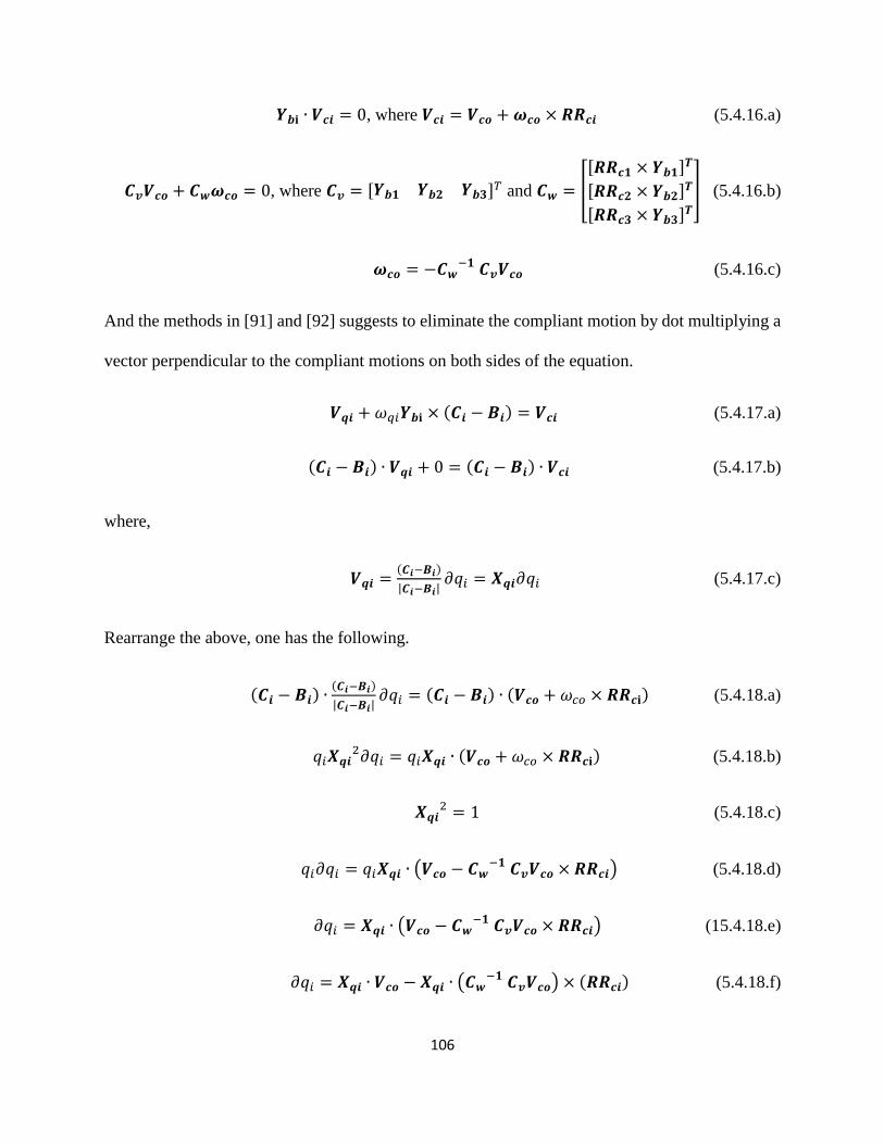
106

𝒀𝒃𝐢 ∙ 𝑽𝒄𝒊 = 0, where 𝑽𝒄𝒊 = 𝑽𝒄𝒐 + 𝝎𝒄𝒐 × 𝑹𝑹𝒄𝒊 (5.4.16.a)

𝑪𝒗𝑽𝒄𝒐 + 𝑪𝒘𝝎𝒄𝒐 = 0, where 𝑪𝒗 = [𝒀𝒃𝟏 𝒀𝒃𝟐 𝒀𝒃𝟑]𝑇 and 𝑪𝒘 = [

[𝑹𝑹𝒄𝟏 × 𝒀𝒃𝟏]𝑻

[𝑹𝑹𝒄𝟐 × 𝒀𝒃𝟐]𝑻

[𝑹𝑹𝒄𝟑 × 𝒀𝒃𝟑]𝑻

] (5.4.16.b)

𝝎𝒄𝒐 = −𝑪𝒘−𝟏 𝑪𝒗𝑽𝒄𝒐 (5.4.16.c)

And the methods in [91] and [92] suggests to eliminate the compliant motion by dot multiplying a

vector perpendicular to the compliant motions on both sides of the equation.

𝑽𝒒𝒊 + 𝜔𝑞𝑖𝒀𝒃𝐢 × (𝑪𝒊 − 𝑩𝒊) = 𝑽𝒄𝒊 (5.4.17.a)

(𝑪𝒊 − 𝑩𝒊) ∙ 𝑽𝒒𝒊 + 0 = (𝑪𝒊 − 𝑩𝒊) ∙ 𝑽𝒄𝒊 (5.4.17.b)

where,

𝑽𝒒𝒊 =(𝑪𝒊−𝑩𝒊)

|𝑪𝒊−𝑩𝒊|𝜕𝑞𝑖 = 𝑿𝒒𝒊𝜕𝑞𝑖 (5.4.17.c)

Rearrange the above, one has the following.

(𝑪𝒊 − 𝑩𝒊) ∙(𝑪𝒊−𝑩𝒊)

|𝑪𝒊−𝑩𝒊|𝜕𝑞𝑖 = (𝑪𝒊 − 𝑩𝒊) ∙ (𝑽𝒄𝒐 + 𝜔𝑐𝑜 × 𝑹𝑹𝒄𝐢) (5.4.18.a)

𝑞𝑖𝑿𝒒𝒊2𝜕𝑞𝑖 = 𝑞𝑖𝑿𝒒𝒊 ∙ (𝑽𝒄𝒐 + 𝜔𝑐𝑜 × 𝑹𝑹𝒄𝐢) (5.4.18.b)

𝑿𝒒𝒊2 = 1 (5.4.18.c)

𝑞𝑖𝜕𝑞𝑖 = 𝑞𝑖𝑿𝒒𝒊 ∙ (𝑽𝒄𝒐 − 𝑪𝒘−𝟏 𝑪𝒗𝑽𝒄𝒐 × 𝑹𝑹𝒄𝒊) (5.4.18.d)

𝜕𝑞𝑖 = 𝑿𝒒𝒊 ∙ (𝑽𝒄𝒐 − 𝑪𝒘−𝟏 𝑪𝒗𝑽𝒄𝒐 × 𝑹𝑹𝒄𝒊) (15.4.18.e)

𝜕𝑞𝑖 = 𝑿𝒒𝒊 ∙ 𝑽𝒄𝒐 − 𝑿𝒒𝒊 ∙ (𝑪𝒘−𝟏 𝑪𝒗𝑽𝒄𝒐) × (𝑹𝑹𝒄𝒊) (5.4.18.f)

107

𝜕𝑞𝑖 = 𝑿𝒒𝒊 ∙ 𝑽𝒄𝒐 + 𝑿𝒒𝒊 ∙ (𝑹𝑹𝒄𝒊) × (𝑪𝒘−𝟏 𝑪𝒗𝑽𝒄𝒐) (5.4.18.g)

𝜕𝑞𝑖 = 𝑿𝒒𝒊 ∙ 𝑽𝒄𝒐 + 𝑿𝒒𝒊 × 𝑹𝑹𝒄𝒊 ∙ 𝑪𝒘−𝟏𝑪𝒗𝑽𝒄𝒐 (5.4.18.h)

𝜕𝑞𝑖 = 𝑿𝒒𝒊𝑻 ∙ 𝑽𝒄𝒐 + (𝑿𝒒𝒊 × 𝑹𝑹𝒄𝒊)

𝑻∙ (𝑪𝒘

−𝟏 𝑪𝒗) ∙ 𝑽𝒄𝒐 (5.4.18.i)

𝜕𝑞𝑖 = (𝑿𝒒𝒊𝑻 + (𝑿𝒒𝒊 × 𝑹𝑹𝒄𝒊)

𝑻∙ (𝑪𝒘

−𝟏 𝑪𝒗)) ∙ 𝑽𝒄𝒐 (5.4.18.j)

𝑱𝒓𝒊 = (𝑿𝒒𝒊 + 𝑿𝒒𝒊 × 𝑹𝑹𝒄𝒊)𝑻∙ (𝑪𝒘

−𝟏 𝑪𝒗) (5.4.18.k)

𝜕𝑞𝑖 = 𝑱𝒓𝒊 ∙ 𝑽𝒄𝒐 (5.4.18.l)

The Jacobian matrix is obtained as below.

𝑱 = [𝑱𝒓𝟏 𝑱𝒓𝟐 𝑱𝒓𝟑]𝑇 (5.4.19.a)

This reflects the relationship between actuation velocities and the end effector velocities.

[𝜕𝑞1 𝜕𝑞2 𝜕𝑞3]𝑇 = 𝑱[𝜕𝑥𝑐 𝜕𝑦𝑐 𝜕𝑧𝑐]

𝑇 (5.4.19.b)

Stiffness of end effector 𝑲𝒄 is expressed as below, where 𝑲𝒒 is the actuation stiffness.

𝑲𝒄 = 𝑱𝑻𝑲𝒒𝑱 , where 𝑲𝒒 = [

𝑘𝑞1 0 0

0 𝑘𝑞2 0

0 0 𝑘𝑞3

] (5.4.20)

The stiffness along 𝑿𝒐, 𝒀𝒐 and 𝒁𝒐 are given.

𝑘𝑥 = (𝑲𝒄𝑿𝒐)𝑻 ∙ 𝑿𝒐; 𝑘𝑦 = (𝑲𝒄𝒀𝒐)

𝑻 ∙ 𝒀𝒐; 𝑘𝑧 = (𝑲𝒄𝒁𝒐)𝑻 ∙ 𝒁𝒐 (5.4.21)

When 𝑿𝒐 rotates around 𝒁𝒐 by φ𝒛, it forms a new vector 𝑿𝛗. The vector 𝑿𝒐 expressed in coordinate

with 𝑿𝛗 is given below.

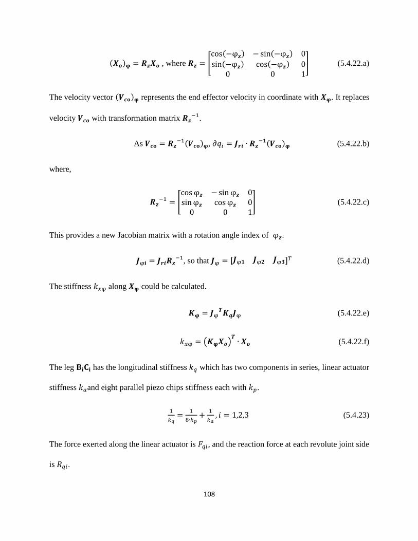
108

(𝑿𝒐)𝛗 = 𝑹𝒛𝑿𝒐 , where 𝑹𝒛 = [cos(−φ𝒛) − sin(−φ𝒛) 0

sin(−φ𝒛) cos(−φ𝒛) 00 0 1

] (5.4.22.a)

The velocity vector (𝑽𝒄𝐨)𝛗 represents the end effector velocity in coordinate with 𝑿𝛗. It replaces

velocity 𝑽𝒄𝒐 with transformation matrix 𝑹𝒛−1.

As 𝑽𝒄𝐨 = 𝑹𝒛−1(𝑽𝒄𝐨)𝛗, 𝜕𝑞𝑖 = 𝑱𝒓𝒊 ∙ 𝑹𝒛

−1(𝑽𝒄𝐨)𝛗 (5.4.22.b)

where,

𝑹𝒛−1 = [

cosφ𝒛 −sin φ𝒛 0sinφ𝒛 cosφ𝒛 0

0 0 1] (5.4.22.c)

This provides a new Jacobian matrix with a rotation angle index of φ𝒛.

𝑱φ𝐢 = 𝑱𝒓𝒊𝑹𝒛−1, so that 𝑱φ = [𝑱φ𝟏 𝑱φ𝟐 𝑱φ𝟑]𝑇 (5.4.22.d)

The stiffness 𝑘𝑥φ along 𝑿𝛗 could be calculated.

𝑲𝛗 = 𝑱φ𝑻𝑲𝒒𝑱φ (5.4.22.e)

𝑘𝑥φ = (𝑲𝛗𝑿𝒐)𝑻∙ 𝑿𝒐 (5.4.22.f)

The leg 𝐁𝐢𝐂𝐢 has the longitudinal stiffness 𝑘𝑞 which has two components in series, linear actuator

stiffness 𝑘𝑎and eight parallel piezo chips stiffness each with 𝑘𝑝.

1

𝑘𝑞=

1

8∙𝑘𝑝+

1

𝑘𝑎, 𝑖 = 1,2,3 (5.4.23)

The force exerted along the linear actuator is 𝐹𝑞𝑖, and the reaction force at each revolute joint side

is 𝑅𝑞𝑖.

109

𝐹𝑞𝑖 = 2𝑅𝑞𝑖, 𝑖 = 1,2,3 (5.4.24.a)

Each piece of the chip takes a share of the load. Eight chips of each leg are connected in parallel,

and each piece of the chip is seen as a cantilever [159]. Its stiffness is the ratio of load to deflection.

𝐹 =𝐹𝑞𝑖

8 (5.4.24.b)

𝑘𝑝 =𝐹

𝑑𝑚𝑎𝑥 (5.4.24.c)

The maximum deflection is expressed as below.

𝑑𝑚𝑎𝑥 =𝐹𝑤3

3𝐸𝑝𝑧𝑡𝐼 (5.4.24.d)

where,

𝐼 =𝑡3ℎ

12 (5.4.24.e)

110

Figure 5.4.5 Leg stiffness. (a) loading and reaction forces; (b) elastic model; (c) Piezo chip size;

(d) loads on piezo chips.

111

5.4.3 Adaption and Operation Optimization

Based on real values of linear actuators and linear tables as selected from manufacturers, so that

numerical analysis can be performed. The design parameters are shown in table 5.4.1.

Table 5.4.1 Design parameters.

Parameters Units Values

ℎ𝑏 𝑚 0.092

𝑟𝑝 𝑚 0.5

𝑟𝑐 𝑚 0.1

ℎ𝑝 𝑚 0.05

[𝑞𝑚𝑖𝑛, 𝑞𝑚𝑎𝑥 ] 𝑚 [0.35, 0.55] 𝛽i, (i=1,2,3) 𝑟𝑎𝑑

[𝜋

2−

𝜋

6

7𝜋

6]

𝛽pj, (j=1,2,3,4) 𝑟𝑎𝑑 [𝜋

4−

𝜋

4−

3𝜋

4

3𝜋

4]

𝛾𝑐𝑚 𝑟𝑎𝑑 0.1745

The original 𝑩𝒊 locations allows the lie-flat configuration but provides a limited workspace.

Genetic algorithm is implemented to find another configuration that enlarges workspace, known

as working configuration. The adjustable design enables the switch between the two

configurations.

The adjustments 𝑏i−𝑎𝑑𝑗 are the variables for the MATLAB optimization algorithm that seeks

global minimum of fitness function 𝑓, while the ultimate aim is to enlarge the workspace index

𝑛𝑒. The optimization process and results are displayed in figure 5.4.6, figure 5.4.7, table 5.4.2 and

table 5.4.3.

𝐗 = [𝑏1−𝑎𝑑𝑗 𝑏2−𝑎𝑑𝑗 𝑏3−𝑎𝑑𝑗] (5.4.25.a)

112

𝑓 = −𝑛𝑒 (5.4.25.b)

Figure 5.4.6 Optimization. (a) genetic algorithm for larger workspace; (b) workspace boundary,

dash: original; solid: optimized.

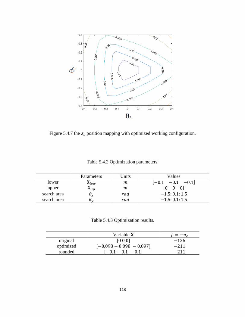
113

Figure 5.4.7 the 𝑧𝑐 position mapping with optimized working configuration.

Table 5.4.2 Optimization parameters.


lower X𝑙𝑜𝑤 𝑚 [−0.1 −0.1 −0.1] upper X𝑢𝑝 𝑚 [0 0 0]

search area 𝜃𝑥 𝑟𝑎𝑑 −1.5: 0.1: 1.5

search area 𝜃𝑦 𝑟𝑎𝑑 −1.5: 0.1: 1.5

Table 5.4.3 Optimization results.

Variable 𝐗 𝑓 = −𝑛𝑒

original [0 0 0] −126

optimized [−0.098 − 0.098 − 0.097] −211

rounded [−0.1 − 0.1 − 0.1] −211

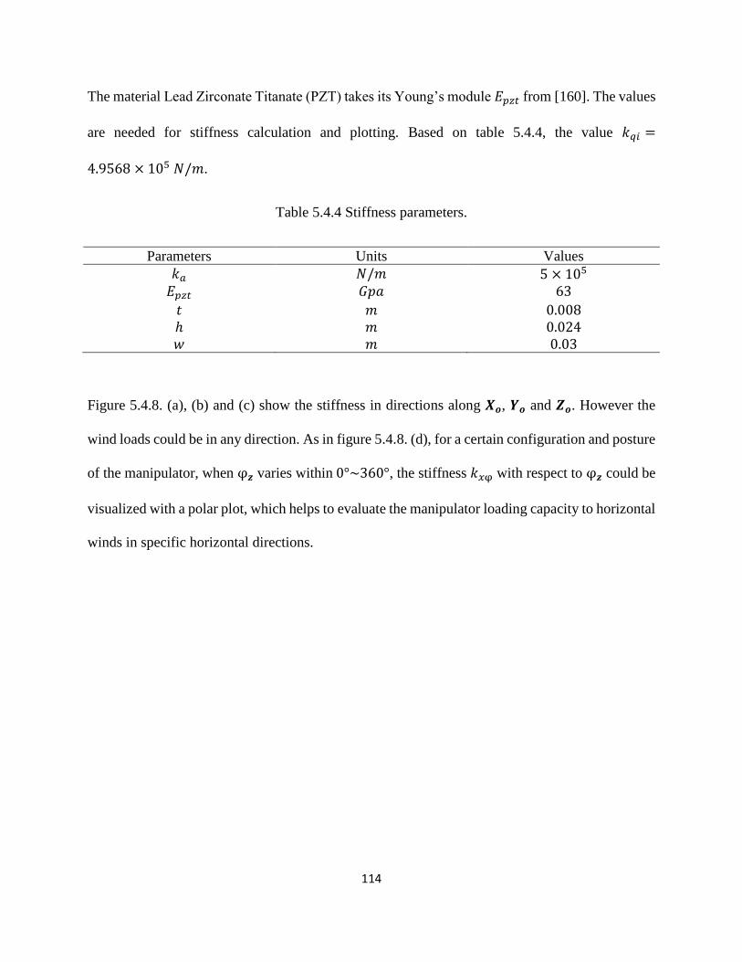
114

The material Lead Zirconate Titanate (PZT) takes its Young’s module 𝐸𝑝𝑧𝑡 from [160]. The values

are needed for stiffness calculation and plotting. Based on table 5.4.4, the value 𝑘𝑞𝑖 =

4.9568 × 105 𝑁/𝑚.

Table 5.4.4 Stiffness parameters.


𝑘𝑎 𝑁/𝑚 5 × 105

𝐸𝑝𝑧𝑡 𝐺𝑝𝑎 63

𝑡 𝑚 0.008

ℎ 𝑚 0.024

𝑤 𝑚 0.03

Figure 5.4.8. (a), (b) and (c) show the stiffness in directions along 𝑿𝒐, 𝒀𝒐 and 𝒁𝒐. However the

wind loads could be in any direction. As in figure 5.4.8. (d), for a certain configuration and posture

of the manipulator, when φ𝒛 varies within 0°~360°, the stiffness 𝑘𝑥φ with respect to φ𝒛 could be

visualized with a polar plot, which helps to evaluate the manipulator loading capacity to horizontal

winds in specific horizontal directions.

115

Figure 5.4.8 Stiffness mappings in prescribed motion range. (a) log(𝑘𝑥) N/m; (b) log(𝑘𝑦) N/m;

(c) log(𝑘𝑧) N/m; (d) stiffness 𝑘𝑥φ polar plot about φ𝑧 𝜃𝑥 = 0.4 and 𝜃𝑦 = −0.5 at working

configuration 𝑿 = [−0.1 − 0.1 − 0.1].


The design of a structural adaptive hybrid harvester enables 3-RPS parallel solar tracker to collect

solar and wind energy at the same time. This design has a lie-flat feature that protects the

116

manipulator from storms, and an enlarged workspace achieved by base joints relocation. This

enables the manipulator to switch between the lie-flat configuration and the working configuration.

Minimum platform height algorithm has been developed and demonstrated to find all eligible

orientations of the platform. Stiffness mappings of the manipulator are plotted, after being

converted to a polar plot, it assists to evaluate its capability to take wind loads in specific horizontal

directions that is significant for lie-flat protection strategy against storms. The design adds

favorable features to solar trackers that improves the energy collection efficiency and operational

safety of the green industry.


This chapter discusses the re-design of 2R1T parallel mechanisms to be deployable structures in

applications of the solar tracking. Two adaptive manipulators are designed.

The first 3-PRS parallel manipulator gives a concept of the deployable re-design, while the second

3-RPS parallel manipulator considers more practical requirements such as dust-proof

requirements, rail loading condition and actuator installation sizes. The deformation of piezo chips

in 3-RPS occurs as a kinematic redundancy which doesn’t affect the end effector degree of

freedom.

On the design and analysis, this chapter introduces the vector diagram method to determine the

folded pose of the structure. It then develops minimum platform height algorithm and Jacobian

matrix transformation to assist the design evaluation.

117

The optimization of the 3-PRS is multi-objective for purpose of specific operation, where both

workspace and general stiffness in selected area are cost functions. (There is another pre-

optimization that determines its basic design parameters for larger workspace).

The optimization of the 3-RPS is single-objective where only workspace is cost function. The

adaption is involved in the operation optimization for large workspace at working configuration.

With the Jacobian transformation matrix developed in 3-RPS model, the 3-PRS model could also

adopt this matrix as cost function to optimize the overall stiffness horizontally or in a specific

direction seasonally.

The designs could also be considered for applications in radar signal receiver/tracker.

118

Chapter 6 Deployable Higher DOF Parallel Manipulators


This chapter expands the deployable design to higher DOF mechanisms. A 6-DOF and a 5-DOF

parallel manipulator with deployable function are designed and analyzed. The link interference

problems are discussed in this chapter.


The manipulators are designed with the required DOF. According to the motion sets intersection,

the motion of the end effector is the intersection of the limb motions. The limbs are in mobile

vertical planes to be deployable, interference free and convenient for kinematic calculation. To

avoid the motion limitation of spherical joints and to actuate the vertical planes with parallel

actuation, an (2-RR)UU 6-DOF limb is designed which is different from the (2-RR)UU limb in

[66] as the (2-RR)UU limb hereby is in vertical planes perpendicular to the base, while the other

(2-RR)UU limb is equivalent to an (2-RR)SR which is perpendicular to the moving platform.

The 6-DOF (2-RR)UU hybrid limbs are in mobile vertical planes actuated on horizontal planes

with parallel actuation instead of serial actuation. Parallel actuation evenly distributes loads and

also reduces bending deformation by vertical loads. A 6-DOF limb doesn’t constraint the end

effector degrees of freedom. The 6-DOF manipulator has three identical 6-DOF (2-RR)UU limbs,

while the 5-DOF manipulator has two 6-DOF (2-RR)UU limbs and a third limb of 5-DOF which

reflect the DOF of the manipulator.

119

The limbs are arranged in vertical planes to avoid interference while the actuation links on

horizontal plane need to be checked to be interference free. The links on horizontal plane are

distributed to parallel layers to avoid interference, but in the same layer the links need to be

checked for interference. Pentagon identification, point-line criteria and link boundary method

have been developed to detect link to link interference.

Jacobian matrix is modified to reflect the stiffness in directions other than the global coordinate

axes. It is also taken to verify the DOF of the novel structures developed in this chapter.

Multi objective optimization of workspace in different orientation of the platform are conducted

where the folded height is among the objectives of the optimization.

6.3 Novel Design of 6-DOF 3T3R Parallel Mechanism

A novel 3-[(2-RR)UU] 6-DOF parallel manipulator is designed with limbs in mobile vertical

planes, that provides larger workspace, less chance of link interference and simplified kinematic

analysis. The link interference detection by pentagon identification and point-line criteria is

demonstrated. Workspace is optimized by different orientations. The Jacobian matrix by global

cartesian coordinate system is developed. A transformation matrix could convert that to Jacobian

matrix of a new coordinate system.

6.3.1 The 3-[(2-RR)UU] Mechanism Design

The 3-RRUU parallel manipulator has 6 DOFs. Figure 6.3.1 shows (a) structure and (b) the

kinematic chains represented by topology diagram [44] [45] with serial actuation. Figure 6.3.2

120

shows an equivalent structure but adopts parallel actuation which provides an even load

distribution of the two actuators on one limb. Besides, the parallel actuation on horizontal plane

forms a stronger cantilever than serial actuation. The latter is selected for the design.

A structure could also be expressed by a notation [48]. Therefore the structure is denoted as 3-[(2-

RR)UU], where underlined joints are actuated. Each limb has two motors 𝐴[𝐴𝑝𝑖] and 𝐴[𝐴𝑞𝑖] in

hybrid chain. This increases the precision and reduces the bending of links 𝐵[B𝑝𝑖], 𝐵[B𝑞𝑖], 𝐵[C𝑝𝑖]

and 𝐵[C𝑞𝑖]. The revolute joints 𝑅[𝐴𝑝𝑖] and 𝑅[𝐴𝑞𝑖] are driven. The revolute joint 𝑅[𝐶𝑖] connects to the

universal joint 𝑈[𝐷𝑖] which consists two revolute joints and one of these is colinear to 𝑅[𝐶𝑖].

The five bar planar mechanisms [161] are serving as the parallel actuation on horizontal plane for

the mobile vertical planes.

121

Figure 6.3.1 Serial actuation.

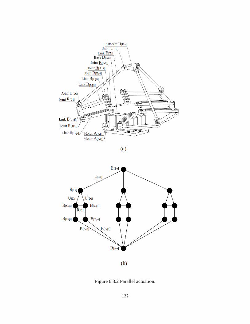
122

Figure 6.3.2 Parallel actuation.

123


Here gives the calculation of link positions, and detection of link interference.

The global cartesian coordinate is at base center 𝑨𝒐: [0 0 0]𝑇 (figure 6.3.3. (a)).

𝑿𝒐 = [1 0 0]𝑇, 𝒀𝒐 = [0 1 0]𝑇, 𝒁𝒐 = [0 0 1]𝑇 (6.3.1)

𝑨𝒑𝒊 = 𝑟𝑏[cos(𝛼𝑖 − 𝛽) sin(𝛼𝑖 − 𝛽) 0]𝑇 (6.3.2.a)

𝑨𝒒𝒊 = 𝑟𝑏[cos(𝛼𝑖 + 𝛽) sin(𝛼𝑖 + 𝛽) 0]𝑇 (6.3.2.b)

The pose of the moving platform (an equilateral triangle) is defined by its orientation 𝜽𝒆 and

position 𝑬𝒐 from global coordinate.

𝜽𝒆 = [𝜃𝑥 𝜃𝑦 𝜃𝑧]𝑇 and 𝑬𝒐 = [𝑥𝑒 𝑦𝑒 𝑧𝑒]𝑇 (6.3.3)

Let 𝜃𝑒 = √𝜃𝑥2 + 𝜃𝑦

2 + 𝜃𝑧2, so that 𝑢𝑥 = 𝜃𝑥/𝜃𝑒, 𝑢𝑦 = 𝜃𝑦/𝜃𝑒, 𝑢𝑧 = 𝜃𝑧/𝜃𝑒.

With orientation matrix 𝑅, the positions 𝑬𝒊 are calculated, where the universal joints are located

with one rotational axis along symmetry lines 𝑬𝒊𝑬𝒐 and the other rotational axis along 𝒀𝒅𝒊. The

platform has a normal vector 𝑵𝒆 that points upward.

𝑹 = [

c𝜃𝑒 + 𝑢𝑥2(1 − c 𝜃𝑒) 𝑢𝑥𝑢𝑦(1 − c 𝜃𝑒) − 𝑢𝑧 s 𝜃𝑒 𝑢𝑥𝑢𝑧(1 − c 𝜃𝑒) + 𝑢𝑦 s 𝜃𝑒

𝑢𝑥𝑢𝑦(1 − c 𝜃𝑒) + 𝑢𝑧 s 𝜃𝑒 c 𝜃𝑒 + 𝑢𝑦2(1 − c 𝜃𝑒) 𝑢𝑦𝑢𝑧(1 − c𝜃𝑒) − 𝑢𝑥 s 𝜃𝑒

𝑢𝑥𝑢𝑧(1 − c 𝜃𝑒) − 𝑢𝑦 s 𝜃𝑒 𝑢𝑦𝑢𝑧(1 − c𝜃𝑒) + 𝑢𝑥 s 𝜃𝑒 c 𝜃𝑒 + 𝑢𝑧2(1 − c𝜃𝑒)

] (6.3.4)

𝑬𝒊 = 𝑹𝑟𝑒[cos(𝛼𝑖) sin(𝛼𝑖) 0]𝑇 + 𝑬𝒐 (6.3.5)

𝑵𝒆 =𝑬𝒐𝑬𝟏×𝑬𝒐𝑬𝟐

|𝑬𝒐𝑬𝟏×𝑬𝒐𝑬𝟐| (6.3.6)

124

𝒀𝒅𝒊 =𝒁𝒐×𝑬𝒐𝑬𝒊

|𝒁𝒐×𝑬𝒐𝑬𝒊| and 𝑿𝒅𝒊 = 𝒀𝒅𝒊 × 𝒁𝒐 (6.3.7)

Figure 6.3.3 Kinematics analysis.

125

Figure 6.3.4 Horizontal plane.

As in figure 6.3.3. (b), the universal joints located at 𝑬𝒊 and 𝑫𝒊 each has a rotational axis along

𝒀𝒅𝒊. Links 𝑬𝒊𝑫𝒊 and lines 𝑬𝒊𝑬𝒐 lie in plane 𝐵𝑖 which is perpendicular to horizontal plane C and

126

horizontal plane D. Let 𝑬𝒊 be projected along −𝒁𝒐 on plane D at 𝑫𝒆𝒊, where 𝑬𝒐𝑫𝒆𝒐 is the

intersecting line of plane 𝐵1 , plane 𝐵2 and plane 𝐵3. One obtains ℎ𝑖 and 𝑏𝑖 in plane 𝐵𝑖.

ℎ𝑖 = 𝑬𝒊 ∙ 𝒁𝒐 − 𝑑 (6.3.8.a)

𝑏𝑖 = √𝑒2 − ℎ𝑖2 (6.3.8.b)

Position 𝑫𝒊 indicates where the universal joint is located. The universal joint has one rotational

axis along 𝒁𝒐 and the other rotational axis along 𝒀𝒅𝒊. As in figure 6.3.4. (a), let the five-bar

mechanisms be in the plane C where the limbs are actuated. The position 𝑪𝒊 indicates the location

of revolute joint. The revolute joints rotate around 𝒁𝒐, and colinear with the universal joints at 𝑫𝒊.

𝑫𝒊 = 𝑬𝒊 + 𝑏𝑖𝑿𝒅𝒊 − ℎ𝑖𝒁𝒐 (6.3.9)

𝑪𝒊 = 𝑫𝒊 − 𝑑𝒁𝒐 (6.3.10)

The 𝑩𝒑𝒊 and 𝑩𝒒𝒊 represent the locations of two revolute joints, rotational axis along 𝒁𝒐.

𝑝𝑖 = |𝑨𝒑𝒊𝑪𝒊| and 𝑞𝑖 = |𝑨𝒒𝒊𝑪𝒊| (6.3.11.a)

𝛾𝑝𝑖 = cos−1 (𝑏2+𝑝𝑖

2−𝑐2

2𝑏𝑝𝑖) and 𝛾𝑞𝑖 = cos−1 (

𝑏2+𝑞𝑖2−𝑐2

2𝑏𝑞𝑖) (6.3.11.b)

𝑹𝒑𝒊 = [

cos 𝛾𝑝𝑖 sin 𝛾𝑝𝑖 0

− sin 𝛾𝑝𝑖 cos 𝛾𝑝𝑖 0

0 0 1

] and 𝑹𝒒𝒊 = [

cos 𝛾𝑞𝑖 −sin 𝛾𝑞𝑖 0

sin 𝛾𝑞𝑖 cos 𝛾𝑞𝑖 0

0 0 1

] (6.3.11.c)

𝑩𝒑𝒊 = 𝑹𝒑𝒊(𝑨𝒑𝒊𝑪𝒊)𝑏

𝑝𝑖+ 𝑨𝒑𝒊 and 𝑩𝒒𝒊 = 𝑹𝒒𝒊(𝑨𝒒𝒊𝑪𝒊)

𝑏

𝑞𝑖+ 𝑨𝒒𝒊 (6.3.11.d)

One could calculate actuation angles 𝛼𝑝𝑖 and 𝛼𝑞𝑖 by 𝑨𝒑𝒊𝑩𝒑𝒊 or 𝑨𝒒𝒊𝑩𝒒𝒊.

127

There are some literatures [68] [48] [126] [130] [162] discussing the link interference detection,

where the main algorithm is to keep safe distance between links. One needs to check that three

five-bar mechanisms have no link interference. The interference detection in this analysis has three

sections.

Section 1 is to limit 𝛼𝑝𝑖 and 𝛼𝑞𝑖 ranges so that the moving sides of the link will not collide with

the base arc of a neighboring link. Such as in figure 6.3.5. (a), the side of 𝑨𝒒𝟏𝑩𝒒𝟏 interferes with

the arc of 𝑨𝒑𝟏. Let 𝑎𝑖𝑛 = 2𝑟𝑎 sin 𝛽 and 𝑎𝑒𝑥 = 2𝑟𝑎 sin (𝜋

3− 𝛽) that are the lengths of hexagon sides.

One needs to verify that 𝑎𝑖𝑛 > 2𝑟𝑚 and 𝑎𝑒𝑥 > 2𝑟𝑚 so that it has enough distance for two motors

with radius 𝑟𝑚.

𝑎𝑚𝑖𝑛 = √𝑏2 + 4𝑟𝑏2 and 𝑎𝑚𝑎𝑥 = 𝑏 + 2𝑟𝑏 (6.3.12.a)

𝛾𝑖𝑛 = 𝑔(𝑎𝑖𝑛) and 𝛾𝑒𝑥 = 𝑔(𝑎𝑒𝑥) (6.3.12.b)

Table 6.3.1 gives 𝛾𝑖𝑛 and 𝛾𝑒𝑥 as offsets on 𝛼𝑝𝑖 and 𝛼𝑞𝑖, to be interference free for section 1.

𝛼𝑝𝑖 𝑎𝑛𝑑 𝛼𝑞𝑖 ∈ [ 𝛾𝑖𝑛,240

180𝜋 − 𝛾𝑒𝑥] (6.3.12.c)

Table 6.3.1 Angles offsets.

Conditions 𝑔(𝑎𝑥)

𝑎𝑥 ∈ (0, 𝑎𝑚𝑖𝑛] sin−1 (

2𝑟𝑏𝑎𝑥

)

𝑎𝑥 ∈ [𝑎𝑚𝑖𝑛 , 𝑎𝑚𝑎𝑥] cos−1 (

𝑏2 + 𝑎𝑥2 − 4𝑟𝑏

2

2 ∙ 𝑎𝑥 ∙ 𝑏)

𝑎𝑥 ∈ [𝑎𝑚𝑎𝑥 , ∞) 0

128

Section 2 is to wipe out the conditions where 𝛼𝑝𝑖 and 𝛼𝑞𝑖 are within ranges but there exists

intersection of links in a loop (see loop 1 and loop 2 in figure 6.3.4. (b)). An algorithm of pentagon

identification could easily find intersection. For concave or convex pentagons, the sum 𝜃𝑖 should

be 3𝜋 to be interference free for section 2.

𝜃𝑖 = 𝛼𝑝𝑖 + 𝛽𝑞𝑖 + 𝛼𝑝𝑖 + 𝛽𝑞𝑖 + 𝛾𝑖 (6.3.13)

Section 3 is to avoid the moving arc of a link interfering with the moving side of a link in another

loop. Such as in figure 6.3.5. (b), the arc of 𝑩𝒑𝟏 interferes with the side of 𝑨𝒒𝟑𝑩𝒒𝟑. For when

𝛼𝑝𝑖 + 𝛼𝑞𝑘 > 5𝜋 3⁄ (𝑖 and 𝑘 index two loops in clockwise order), the point-line criteria could

conveniently check the distance between the two. The link 𝑩𝒑𝒊𝑪𝒊 or 𝑩𝒒𝒊𝑪𝒊 are in different

horizontal layers, thus are exempted form examination. The point-line criteria in table 6.3.2 need

to be met to be interference free for section 3. For example, a point 𝑩𝒑𝒊 should be a distance 𝑟𝑏

away from line 𝑨𝒒𝒌𝑩𝒒𝒌, when 𝛼𝑝𝑖 > 𝛼𝑞𝑘.

Table 6.3.2 Point-line criteria.

Conditions Criteria

𝛼𝑝𝑖 > 𝛼𝑞𝑘 𝒁𝒐 ∙ (𝑩𝒑𝒊𝑨𝒒𝒌 × 𝑩𝒑𝒊𝑩𝒒𝒌) − 2𝑟𝑏𝑏 > 0

𝛼𝑝𝑖 < 𝛼𝑞𝑘 𝒁𝒐 ∙ (𝑩𝒒𝒌𝑩𝒑𝒊 × 𝑩𝒒𝒌𝑨𝒑𝒊) − 2𝑟𝑏𝑏 > 0

129

Figure 6.3.5 Interference detection.

130

In figure 6.3.6. (a), from the global cartesian coordinate at 𝑨𝒐, the moving platform center 𝑬𝒐 has

a linear velocity 𝒗𝒆𝒐 and an angular velocity 𝝎𝒆𝒐, that contribute to the linear velocity at 𝑬𝒊. The

linear velocity at 𝑫𝒊 could be divided to 𝒗𝒙𝒅𝒊 and 𝒗𝒚𝒅𝒊, which are along 𝑿𝒅𝒊 and 𝒀𝒅𝒊 respectively.

A method of dot multiplication [91] [92] can be used since 𝒗𝒙𝒅𝒊 is not perpendicular to 𝑬𝒊𝑫𝒊.

𝑬𝒊𝑫𝒊 ∙ (𝒗𝒆𝒐 + 𝝎𝒆𝒐 × 𝑬𝒐𝑬𝒊) = 𝑬𝒊𝑫𝒊 ∙ 𝒗𝒙𝒅𝒊 (6.3.14.a)

So that

𝒗𝒙𝒅𝒊 =𝑬𝒊𝑫𝒊∙(𝒗𝒆𝒐+𝝎𝒆𝒐×𝑬𝒐𝑬𝒊)

𝑬𝒊𝑫𝒊∙𝑿𝒅𝒊∙ 𝑿𝒅𝒊 (6.3.14.b)

The angular velocity 𝝎𝒆𝒐 could be divided to 𝝎𝒆𝒊, 𝝎𝒚𝒊 and 𝝎𝒛𝒊, that are along 𝑬𝒐𝑬𝒊, 𝒀𝒅𝒊 and 𝒁𝒐

respectively. Components 𝝎𝒆𝒊 and 𝝎𝒚𝒊 have no contribution to 𝒗𝒚𝒅𝒊, except 𝝎𝒛𝒊.

𝒗𝒆𝒐 ∙ 𝒀𝒅𝒊 ∙ 𝒀𝒅𝒊 + 𝝎𝒛𝒊 × 𝑬𝒐𝑫𝒊 = 𝒗𝒚𝒅𝒊 (6.3.15.a)

where

𝝎𝒛𝒊 = (𝝎𝒆𝒐 ∙ 𝒁𝒐 −𝑬𝒐𝑬𝒊∙𝒁𝒐

𝑬𝒐𝑬𝒊∙𝑿𝒅𝒊∙ 𝝎𝒆𝒐 ∙ 𝑿𝒅𝒊) ∙ 𝒁𝒐 (6.3.15.b)

So that

𝒗𝒚𝒅𝒊 = 𝒗𝒆𝒐 ∙ 𝒀𝒅𝒊 ∙ 𝒀𝒅𝒊 + (𝝎𝒆𝒐 ∙ 𝒁𝒐 −𝑬𝒐𝑬𝒊∙𝒁𝒐

𝑬𝒐𝑬𝒊∙𝑿𝒅𝒊∙ 𝝎𝒆𝒐 ∙ 𝑿𝒅𝒊) ∙ 𝒁𝒐 × 𝑬𝒐𝑫𝒊 (6.3.15.c)

The angular velocity 𝜔𝑝𝑖 ∙ 𝒁𝒐 and 𝜔𝑞𝑖 ∙ 𝒁𝒐 are the actuation angular velocities at 𝑨𝒑𝒊 and 𝑨𝒒𝒊.

𝑩𝒑𝒊𝑪𝒊 ∙ (𝒗𝒙𝒅𝒊 + 𝒗𝒚𝒅𝒊) = 𝑩𝒑𝒊𝑪𝒊 ∙ (𝒁𝒐 × 𝑨𝒑𝒊𝑩𝒑𝒊) ∙ 𝜔𝑝𝑖 (6.3.16)

131

So that,

𝜔𝑝𝑖 = 𝑱𝒑𝒗𝒊𝑇 ∙ 𝒗𝒆𝒐 + 𝑱𝒑𝒘𝒊

𝑇 ∙ 𝝎𝒆𝒐 (6.3.17.a)

where,

𝑱𝒑𝒗𝒊 =𝑩𝒑𝒊𝑪𝒊∙𝑿𝒅𝒊

𝑩𝒑𝒊𝑪𝒊∙(𝒁𝒐×𝑨𝒑𝒊𝑩𝒑𝒊)∙

𝑬𝒊𝑫𝒊

𝑬𝒊𝑫𝒊∙𝑿𝒅𝒊+

𝑩𝒑𝒊𝑪𝒊∙𝒀𝒅𝒊∙𝒀𝒅𝒊

𝑩𝒑𝒊𝑪𝒊∙(𝒁𝒐×𝑨𝒑𝒊𝑩𝒑𝒊) (6.3.17.b)

𝑱𝒑𝒘𝒊 =𝑩𝒑𝒊𝑪𝒊∙𝑿𝒅𝒊

𝑩𝒑𝒊𝑪𝒊∙(𝒁𝒐×𝑨𝒑𝒊𝑩𝒑𝒊)∙𝑬𝒊𝑫𝒊×𝑬𝒊𝑬𝒐

𝑬𝒊𝑫𝒊∙𝑿𝒅𝒊+

𝑩𝒑𝒊𝑪𝒊∙(𝒁𝒐×𝑬𝒐𝑫𝒊)∙𝒁𝒐

𝑩𝒑𝒊𝑪𝒊∙(𝒁𝒐×𝑨𝒑𝒊𝑩𝒑𝒊)−

𝑬𝒐𝑬𝒊∙𝒁𝒐

𝑬𝒐𝑬𝒊∙𝑿𝒅𝒊∙𝑩𝒑𝒊𝑪𝒊∙(𝒁𝒐×𝑬𝒐𝑫𝒊)∙𝑿𝒅𝒊

𝑩𝒑𝒊𝑪𝒊∙(𝒁𝒐×𝑨𝒑𝒊𝑩𝒑𝒊) (6.3.17.c)

Figure 6.3.6 Jacobian matrix analysis.

One could have the similar for 𝜔𝑞𝑖, 𝑱𝒒𝒗𝒊 and 𝑱𝒒𝒘𝒊. The Jacobian matrix is obtained as below.

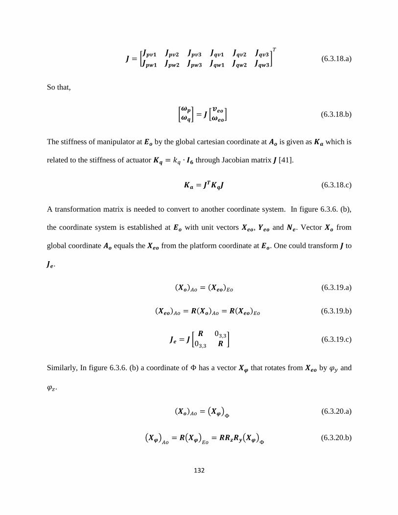
132

𝑱 = [𝑱𝒑𝒗𝟏 𝑱𝒑𝒗𝟐 𝑱𝒑𝒗𝟑

𝑱𝒑𝒘𝟏 𝑱𝒑𝒘𝟐 𝑱𝒑𝒘𝟑

𝑱𝒒𝒗𝟏 𝑱𝒒𝒗𝟐 𝑱𝒒𝒗𝟑

𝑱𝒒𝒘𝟏 𝑱𝒒𝒘𝟐 𝑱𝒒𝒘𝟑]

𝑇

(6.3.18.a)

So that,

[𝝎𝒑

𝝎𝒒] = 𝑱 [

𝒗𝒆𝒐

𝝎𝒆𝒐] (6.3.18.b)

The stiffness of manipulator at 𝑬𝒐 by the global cartesian coordinate at 𝑨𝒐 is given as 𝑲𝒂 which is

related to the stiffness of actuator 𝑲𝒒 = 𝑘𝑞 ∙ 𝑰𝟔 through Jacobian matrix 𝑱 [41].

𝑲𝒂 = 𝑱𝑻𝑲𝒒𝑱 (6.3.18.c)

A transformation matrix is needed to convert to another coordinate system. In figure 6.3.6. (b),

the coordinate system is established at 𝑬𝒐 with unit vectors 𝑿𝒆𝒐, 𝒀𝒆𝒐 and 𝑵𝒆. Vector 𝑿𝒐 from

global coordinate 𝑨𝒐 equals the 𝑿𝒆𝒐 from the platform coordinate at 𝑬𝒐. One could transform 𝑱 to

𝑱𝒆.

(𝑿𝒐)𝐴𝑜 = (𝑿𝒆𝒐)𝐸𝑜 (6.3.19.a)

(𝑿𝒆𝒐)𝐴𝑜 = 𝑹(𝑿𝒐)𝐴𝑜 = 𝑹(𝑿𝒆𝒐)𝐸𝑜 (6.3.19.b)

𝑱𝒆 = 𝑱 [𝑹 03,3

03,3 𝑹] (6.3.19.c)

Similarly, In figure 6.3.6. (b) a coordinate of Φ has a vector 𝑿𝝋 that rotates from 𝑿𝒆𝒐 by 𝜑𝑦 and

𝜑𝑧.

(𝑿𝒐)𝐴𝑜 = (𝑿𝝋)Φ

(6.3.20.a)

(𝑿𝝋)𝐴𝑜

= 𝑹(𝑿𝝋)𝐸𝑜

= 𝑹𝑹𝒛𝑹𝒚(𝑿𝝋)Φ

(6.3.20.b)

133

𝑹𝒛 = [cos𝜑𝑧 −sin𝜑𝑧 0sin 𝜑𝑧 cos𝜑𝑧 0

0 0 1] and 𝑹𝒚 = [

cos𝜑𝑦 0 sin𝜑𝑦

0 1 0− sin𝜑𝑦 0 cos𝜑𝑦

] (6.3.20.c)

A vector in coordinate 𝑨𝒐 could be converted to that in coordinate Φ. One could transform 𝑱 to 𝑱𝜑.

𝑱𝜑 = 𝑱 [𝑹𝑹𝒛𝑹𝒚 03,3

03,3 𝑹𝑹𝒛𝑹𝒚] (6.3.20.d)

𝑲𝝋 = 𝑱𝜑𝑻𝑲𝒒𝑱𝜑 (6.3.20.e)

6.3.3 Multi-objective Design Optimization

The workspace is evaluated by setting three orientations 𝜽𝒆𝒋 (𝑗 = 1,2,3) of the platform, and then

searching for all eligible positions of the 𝑬𝒐 within the searching ranges. The number 𝑛𝑒𝑗 of the

eligible positions indicate the volume of the workspace by orientation 𝜽𝒆𝒋.

Considering the efficiency of workspace (largest workspace made by minimum limb sizes), cost

function 𝑓𝑗 is taken. Pareto method [104] is used to search for the best result of each cost function

with non-sacrifice to another cost function.

𝑓𝑗 = −𝑛𝑒𝑗

(∑ 𝑥𝑖5𝑖=1 )

3 (6.3.21)

The basic modeling parameters are given in table 6.3.3. Table 6.3.4 gives the ranges of the

optimization variables 𝑥1~𝑥6, considering that each revolute or universal joint is at least 0.05 m

from the center of a body it connects to. Table 6.3.5 gives the three orientations, and the 𝑬𝒐 search

ranges by each orientation.

134

Table 6.3.6 shows the results of the optimization and the cost function value, where 𝐹 = 𝑓1 + 𝑓2 +

𝑓3. The four results are selected from the final optimization solutions, with result 1 for the best of

𝑓1; result 2 for the best of 𝑓2; result 3 for the best of 𝑓3; and result 4 for the best of 𝐹 overall. The

result 4 is chosen for the full workspace plotting in 𝜽𝒆𝟏, 𝜽𝒆𝟐 and 𝜽𝒆𝟑 in figure 6.3.7.

Table 6.3.3 Modeling parameters.

Parameters Values Units

𝑑 0 𝑚

𝑟𝑏 0.015 𝑚

𝑟𝑐 0.010 𝑚

𝑟𝑚 0.025 𝑚

𝛼𝑖 (4𝑖 − 1) 𝜋 6⁄ 𝑟𝑎𝑑


𝑥1 𝑥2 𝑥3 𝑥4 𝑥5 𝑥6

Variables 𝑒 𝑟𝑒 𝑟𝑎 𝑏 𝑐 𝛽

Ranges [0.1, 0.7] [0.05,0.7] [0.05,0.7] [0.1, 0.7] [0.1,0.7] [𝜋/18, 5𝜋/18] Units 𝑚 𝑚 𝑚 𝑚 𝑚 𝑟𝑎𝑑

Table 6.3.5 Motion and search ranges.

Orientations and positions Values Units

𝜽𝒆𝟏 [0 0 0] 𝑟𝑎𝑑

𝜽𝒆𝟐 [𝜋 6⁄ 0 0] 𝑟𝑎𝑑

𝜽𝒆𝟑 [0 0 𝜋 6⁄ ] 𝑟𝑎𝑑

𝑥𝑒 -0.1: 0.05: 0.1 𝑚

𝑦𝑒 -0.1: 0.05: 0.1 𝑚

𝑧𝑒 0.1: 0.05: 0.3 𝑚

135


𝑥1 𝑥2 𝑥3 𝑥4 𝑥5 𝑥6 𝑓1 𝑓2 𝑓3 𝐹 Result 1 0.361 0.051 0.102 0.207 0.218 0.296 -126.574 -89.204 -94.026 -309.804

Result 2 0.345 0.051 0.102 0.208 0.219 0.303 -119.825 -119.825 -99.644 -339.294

Result 3 0.386 0.051 0.079 0.245 0.232 0.344 -120.724 -85.939 -111.52 -318.179

Result 4 0.348 0.051 0.102 0.205 0.219 0.300 -121.277 -117.488 -101.07 -339.829

Figure 6.3.7 Full workspace in 𝜽𝒆𝟏, 𝜽𝒆𝟐, 𝜽𝒆𝟑 of result 4.

136

Figure 6.3.8 Stiffness mapping 𝜽𝒆 = [15 ∙𝜋

18020 ∙

𝜋

18010 ∙

𝜋

180]𝑇.

As one could calculate the stiffness in or around 𝑿𝝋. The polar stiffness of the end effector center

𝑬𝒐 at any pose could be plotted about rotation angle 𝜑𝑦 and 𝜑𝑧. The unit stiffness in and around

vectors 𝑿𝒐, 𝒀𝒐, 𝒁𝒐 from global coordinate at 𝑨𝒐 are mapped over an area of 𝑬𝒐 = [𝑥𝑒 𝑦𝑒 0.2]𝑇

137

in figure 6.3.8. (a)~(f). The unit stiffness in and around 𝑿𝝋 from given coordinate of Φ is mapped

about angle [𝜑𝑦 𝜑𝑧] when 𝑬𝒐 = [0.1 0.1 0.2]𝑇 in figure 6.3.8. (g) and (h).


A 3-[(2-RR)UU] 6-DOF parallel manipulator is designed with limbs in mobile vertical planes. The

pentagon identification and point-line criteria are developed for link interference detection. The

workspace boundaries of different orientation angles are plotted. The unit stiffness in and around

the global coordinate vectors are mapped. With a transformation matrix this stiffness could be

converted to indicate stiffness in or around any vector that is a rotation angle from the global

coordinate system.

6.4 Novel Design of 5-DOF 3T2R Parallel Mechanism

There are 5-DOF serial manipulators such as [163] [164], but none has been designed with 3T2R

motion. There is a 3T2R manipulator [165] [166] fully parallel with 5 limbs. Hybrid limbs could

offer larger workspace than fully parallel manipulators.

A novel 5-DOF 3T2R parallel manipulator is designed with chains set in perpendicular planes.

The synthesis design is based on motion sets intersection and disseminated Chebychev-Grübler-

Kutzbach formula. A boundary offset method is developed to detect link interference between

links in a same plane. A multi-objective optimization is practiced on the design for multiple

performance improvements. The Jacobian stiffness based on oriented platform coordinate is

developed. This section also discusses the potential applications of the design.

138

6.4.1 The PRPU Equivalent Mechanism Design

Classical Chebychev-Grübler-Kutzbach formula could determine the degree of freedom (DOF) of

a mechanism.

𝑀 = 6(B − J − 1) + ∑ 𝑑𝑖𝑛𝑖=1 (6.4.1.a)

The classical formula can be disseminated to represent the DOF of platform and limbs separately,

where the platform and base has the initial DOF denoted as 𝑀𝑒𝑜, and the limb chain 𝑖 has its

individual DOF denoted as 𝑀𝑒𝑖 with 𝑑𝑖 for joints. The total DOF of a parallel manipulator is 𝑀.

𝑀 = 𝑀𝑒𝑜 + ∑ 𝑀𝑒𝑖𝑛𝑖=1 (6.4.1.b)

𝑀𝑒𝑜 = 6(2 − 1) = 6 (6.4.1.c)

𝑀𝑒𝑖 = 6(−1) + 𝑑𝑖 (6.4.1.d)

Based on the motion sets intersection of a parallel manipulator, 𝑀 is restricted by min(𝑀𝑒𝑜 + 𝑀𝑒𝑖).

𝑀 = min(𝑀𝑒𝑜 + 𝑀𝑒𝑖) = 𝑑𝑖 (6.4.1.e)

In figure 6.4.1. (a), the motion of a serial limb is the addition from three parts. These are the

motions of the links on horizontal plane Z, the motions of the links on vertical plane X and the

motions of the connection joint which connects plane X and platform. A coordinate system with

𝒙, 𝒚 and 𝒛 axes is set at a point on the intersecting line of plane Z and plane X where they are

jointed. The axis 𝒛 is normal to plane Z, while the axis 𝒚 is along the intersecting line of Plane Z

and plane X.

139

The 𝑅𝑥, 𝑅𝑦 and 𝑅𝑧 represent the rotational motions around 𝒙, 𝒚 and 𝒛 axes. The 𝑇𝑥, 𝑇𝑦 and 𝑇𝑧

represent translational motions along 𝒙, 𝒚 and 𝒛 axes. A series of these symbols in sequence define

the motions of a chain from the base to the end effector (from left to right). There are some

properties of the symbols as to whether they are commutative.

𝑅𝑦𝑅𝑥 ≠ 𝑅𝑥𝑅𝑦 and 𝑇𝑥𝑇𝑦 = 𝑇𝑦𝑇𝑥 (6.4.2.a)

𝑇𝑦𝑅𝑥 ≠ 𝑅𝑥𝑇𝑦 and 𝑇𝑥𝑅𝑥 = 𝑅𝑥𝑇𝑥 (6.4.2.b)

In plane X, normal to 𝒙 axis, 𝑅𝑥3 can be any member of the four members of a set, where each

member includes three motions. The three motions shall be enough to reach any position or rotaion

in plane X. The motions under one bar can change their orders. 𝑅𝑦3 and 𝑅𝑧

3 are similar as 𝑅𝑥3.

𝑅𝑥3 ∈ {𝑇𝑦𝑇𝑧𝑅𝑥

, 𝑇𝑦𝑅𝑥𝑅𝑥 , 𝑇𝑧𝑅𝑥𝑅𝑥

, 𝑅𝑥𝑅𝑥𝑅𝑥} (6.4.2.c)

𝑇𝑥𝑅𝑥3 = 𝑅𝑥

3𝑇𝑥 (6.4.2.d)

𝑅𝑥2 can be any member of the five members of a set, where each member includes two motions.

One could find the properties of the motion groups as below.

𝑅𝑥2 ∈ {𝑇𝑦𝑅𝑥, 𝑅𝑥𝑇𝑦, 𝑇𝑧𝑅𝑥, 𝑅𝑥𝑇𝑧 , 𝑅𝑥𝑅𝑥 } (6.4.2.e)

𝑅𝑥2𝑅𝑦

3 = 𝑅𝑥3𝑅𝑦

2 (6.4.2.f)

The rotational motion group 𝑅𝑥𝑅𝑦𝑅𝑧 exists when the three rotational axes join at one single point

like a spherical joint. The following condition is equivalent to a spherical joint.

𝑅𝑥3 𝑅𝑦𝑅𝑧 = 𝑅𝑥

2𝑅𝑥𝑅𝑦𝑅𝑧 = 𝑇𝑦𝑇𝑧

𝑅𝑥𝑅𝑦𝑅𝑧 (6.4.2.g)

140

To organize a given motion group such as 𝑇𝑥𝑇𝑦𝑇𝑧𝑅𝑥𝑅𝑦 to two perpendicular planes and the

connection point, one needs to define the first plane, the second plane, and the point where second

plane connects to end effector.

Here, motions in first plane (plane Z) could be defined as 𝑃𝑧 ; motions in second plane (plane X)

as 𝑃𝑥 ; and the motions at the connection point as 𝐷�� which can be any of the six members below.

𝐷�� ∈ {𝑅𝑦, 𝑅𝑧 , 𝑅𝑦𝑅𝑥, 𝑅𝑦𝑅𝑧 , 𝑅𝑧𝑅𝑥, 𝑅𝑧𝑅𝑦 } (6.4.2.h)

In table 6.4.1. the 5-DOF chain is the main limb of the manipulator. Its structure is selected as

𝑇𝑥𝑇𝑦𝑅𝑥𝑅𝑥 𝑅𝑦, or known as PRPU as to name the joints.

Table 6.4.1 Motions 𝑇𝑥𝑇𝑦𝑇𝑧𝑅𝑥𝑅𝑦 in 𝑃𝑧 𝑃�� 𝐷��.

𝑃𝑧 𝑃�� 𝐷�� Options

𝑇𝑥 𝑇𝑦𝑇𝑧𝑅𝑥 𝑅𝑦 5

𝑇𝑥 𝑇𝑦𝑅𝑥𝑅𝑥 𝑅𝑦 3

𝑇𝑥 𝑅𝑥𝑅𝑥𝑅𝑥 𝑅𝑦 1

For options of the other two limbs, the (2-RR)UU (𝑅𝑧𝑅𝑧𝑅𝑧 𝑅𝑥𝑅𝑥 𝑅𝑦) chain of 6-DOF is selected.

Figure 6.4.1. (b) shows the topology diagram that represents the whole structure with nodes for

bodies and lines for joints. Figure 6.4.1. (c) and (d) show the manipulator in working and lie-flat

postures. The structure is denoted as PRPU/2-[(2-RR)UU] according to [48]. The linear actuator

(model: DLA-12-40-311-200-IP65) [158] actuates prismatic joint P. The five-bar mechanism

[161] is actuated by worm gear motors (model: 9DCW-120-30) [167] on revolute joint R.

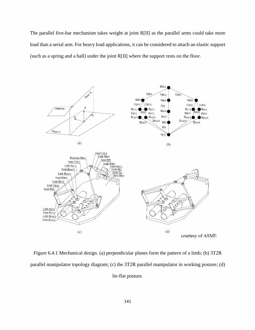
141

The parallel five-bar mechanism takes weight at joint R[II] as the parallel arms could take more

load than a serial arm. For heavy load applications, it can be considered to attach an elastic support

(such as a spring and a ball) under the joint R[II] where the support rests on the floor.

Figure 6.4.1 Mechanical design. (a) perpendicular planes form the pattern of a limb; (b) 3T2R

parallel manipulator topology diagram; (c) the 3T2R parallel manipulator in working posture; (d)

lie-flat posture.

142


Link positions calculation and link interference detection are performed to evaluate the workspace.

Figure 6.4.2 Kinematics analysis. (a) the kinematic analysis; (b) the limbs in vertical planes and

horizontal planes; (c) links on horizontal planes projected on plane O; (d) links on plane B.

143

In figure 6.4.2. (a), the base center is at 𝑶: [0 0 0]𝑇. The 𝑿𝒐, 𝒀𝒐 and 𝒁𝒐 are three orthogonal unit

vectors of the global coordinate.

𝑿𝒐 = [1 0 0]𝑇, 𝒀𝒐 = [0 1 0]𝑇, 𝒁𝒐 = [0 0 1]𝑇 (6.4.3)

The three limbs are in three mobile vertical planes 𝐸1, 𝐸𝑗 (𝑗 = 2,3) in figure 6.4.2. (b).

The platform has 5 DOFs. These are three translational motions 𝑥𝑒𝑿𝒐, 𝑦𝑒𝒀𝒐, 𝑧𝑒𝒁𝒐 and two

orientation motions 𝜃𝑒𝑥𝑿𝒐, 𝜃𝑒𝑦𝒀𝒆, so that 𝑬𝒊 (𝑖 = 1,2,3) are obtained.

𝑬𝒐 = [𝑥𝑒 𝑦𝑒 𝑧𝑒]𝑇 (6.4.4)

𝑬𝒊 = 𝑬𝒐 + 𝑹𝒆𝒙𝑹𝒆𝒚𝑟𝑒𝑖[cos 𝛼𝑒𝑖 sos 𝛼𝑒𝑖 0]𝑇 (6.4.5.a)

Where

𝑹𝒆𝒙 = [1 0 00 cos 𝜃𝑒𝑥 −sin 𝜃𝑒𝑥

0 sin 𝜃𝑒𝑥 cos 𝜃𝑒𝑥

] (6.4.5.b)

𝑹𝒆𝒚 = [

cos 𝜃𝑒𝑦 0 sin 𝜃𝑒𝑦

0 1 0− sin 𝜃𝑒𝑦 0 cos 𝜃𝑒𝑦

] (6.4.5.c)

The oriented coordinate is at 𝑬𝒐 with orthogonal unit vectors 𝑿𝒆, 𝒀𝒆 and 𝑵𝒆.

𝒀𝒆 =1

𝑟𝑒1(𝑬𝒐𝑬𝟏), 𝑿𝒆 = 𝒀𝒆 × 𝑵𝒆, 𝑵𝒆 =

𝑬𝒐𝑬𝟏×𝑬𝒐𝑬𝟐

|𝑬𝒐𝑬𝟏×𝑬𝒐𝑬𝟐| (6.4.6)

Another coordinate is at 𝑬𝒊 with unit vectors 𝑿𝒅𝒊 and 𝒀𝒅𝒊 about vertical planes.

𝒀𝒅𝒊 =𝒁𝒐×𝑬𝒐𝑬𝒊

|𝒁𝒐×𝑬𝒐𝑬𝒊| and 𝑿𝒅𝒊 = 𝒀𝒅𝒊 × 𝒁𝒐 (6.4.7)

Since limb 2 and limb 3 are in mobile vertical planes, the 𝑫𝒋 positions could be obtained.

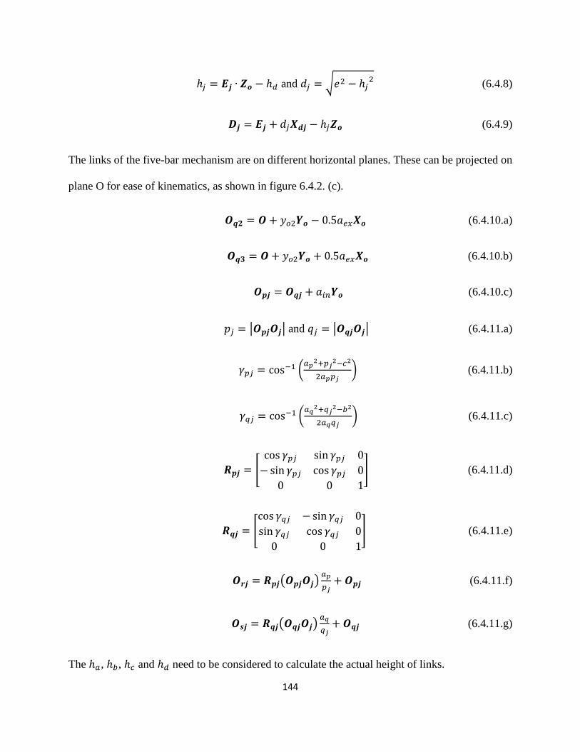
144

ℎ𝑗 = 𝑬𝒋 ∙ 𝒁𝒐 − ℎ𝑑 and 𝑑𝑗 = √𝑒2 − ℎ𝑗2 (6.4.8)

𝑫𝒋 = 𝑬𝒋 + 𝑑𝑗𝑿𝒅𝒋 − ℎ𝑗𝒁𝒐 (6.4.9)

The links of the five-bar mechanism are on different horizontal planes. These can be projected on

plane O for ease of kinematics, as shown in figure 6.4.2. (c).

𝑶𝒒𝟐 = 𝑶 + 𝑦𝑜2𝒀𝒐 − 0.5𝑎𝑒𝑥𝑿𝒐 (6.4.10.a)

𝑶𝒒𝟑 = 𝑶 + 𝑦𝑜2𝒀𝒐 + 0.5𝑎𝑒𝑥𝑿𝒐 (6.4.10.b)

𝑶𝒑𝒋 = 𝑶𝒒𝒋 + 𝑎𝑖𝑛𝒀𝒐 (6.4.10.c)

𝑝𝑗 = |𝑶𝒑𝒋𝑶𝒋| and 𝑞𝑗 = |𝑶𝒒𝒋𝑶𝒋| (6.4.11.a)

𝛾𝑝𝑗 = cos−1 (𝑎𝑝

2+𝑝𝑗2−𝑐2

2𝑎𝑝𝑝𝑗) (6.4.11.b)

𝛾𝑞𝑗 = cos−1 (𝑎𝑞

2+𝑞𝑗2−𝑏2

2𝑎𝑞𝑞𝑗) (6.4.11.c)

𝑹𝒑𝒋 = [

cos 𝛾𝑝𝑗 sin 𝛾𝑝𝑗 0

− sin 𝛾𝑝𝑗 cos 𝛾𝑝𝑗 0

0 0 1

] (6.4.11.d)

𝑹𝒒𝒋 = [

cos 𝛾𝑞𝑗 −sin 𝛾𝑞𝑗 0

sin 𝛾𝑞𝑗 cos 𝛾𝑞𝑗 0

0 0 1

] (6.4.11.e)

𝑶𝒓𝒋 = 𝑹𝒑𝒋(𝑶𝒑𝒋𝑶𝒋)𝑎𝑝

𝑝𝑗+ 𝑶𝒑𝒋 (6.4.11.f)

𝑶𝒔𝒋 = 𝑹𝒒𝒋(𝑶𝒒𝒋𝑶𝒋)𝑎𝑞

𝑞𝑗+ 𝑶𝒒𝒋 (6.4.11.g)

The ℎ𝑎, ℎ𝑏, ℎ𝑐 and ℎ𝑑 need to be considered to calculate the actual height of links.

145

In figure 6.4.2. (d), links 𝑩𝐬𝟐𝑩𝟐 and 𝑩𝐬𝟑𝑩𝟑 are in plane B. The links of the five-bar mechanism

are in different planes. Link interference needs to be checked for links in each plane.

In figure 6.4.3. (a), let’s suppose two links 𝑷𝟏𝑷𝟐 and 𝑸𝟏𝑸𝟐 with boundary of 𝑟𝑝 and 𝑟𝑞 respectively

are in one plane. When boundaries offset is taken, this problem is changed to link 𝑷𝟏𝑷𝟐 with

boundary 𝑟𝑝 + 𝑟𝑞 and a line segment 𝑸𝟏𝑸𝟐. The two shall not interfere with each other. The link

𝑷𝟏𝑷𝟐 with offset boundary will be divided to three areas I, II and III as shown in figure 6.4.3. (c).

Criteria 1, line segment 𝑸𝟏𝑸𝟐 could not touch line segments 𝑺𝟏𝑺𝟐 or 𝑼𝟏𝑼𝟐. Let’s take 𝑸𝟏𝑸𝟐 and

𝑺𝟏𝑺𝟐 for example as shown in figure 6.4.3. (d). The same should be checked for 𝑼𝟏𝑼𝟐.

(𝑺𝟏𝑸𝟏 × 𝑺𝟏𝑸𝟐) ∙ (𝑺𝟐𝑸𝟏 × 𝑺𝟐𝑸𝟐) > 0 (6.4.12.a)

And

(𝑺𝟏𝑸𝟏 × 𝑺𝟐𝑸𝟏) ∙ (𝑺𝟏𝑸𝟐 × 𝑺𝟐𝑸𝟐) > 0 (6.4.12.b)

Criteria 2, line segment 𝑸𝟏𝑸𝟐 could not touch area I or area III. Let’s take 𝑸𝟏𝑸𝟐 and area I for

example as shown in figure 6.4.3. (e). The same should be checked for area III.

When (𝑸𝟏𝑸𝟐 ∙ 𝑸𝟏𝑷𝟏) ∙ (𝑸𝟏𝑸𝟐 ∙ 𝑸𝟐𝑷𝟏) > 0

|𝑸𝟏𝑷𝟏| > 𝑟𝑝 + 𝑟𝑞 ; |𝑸𝟐𝑷𝟏| > 𝑟𝑝 + 𝑟𝑞 (6.4.13.a)

When (𝑸𝟏𝑸𝟐 ∙ 𝑸𝟏𝑷𝟏) ∙ (𝑸𝟏𝑸𝟐 ∙ 𝑸𝟐𝑷𝟏) ≤ 0

|𝑷𝟏𝑸𝟏 × 𝑷𝟏𝑸𝟐| > |𝑸𝟏𝑸𝟐| ∙ (𝑟𝑝 + 𝑟𝑞) (6.4.13.b)

146

Criteria 3, line segment 𝑸𝟏𝑸𝟐 could not touch area II. (figure 6.4.3. (f)). As criteria 1 and 2 have

already been checked, criteria 3 only needs to check that 𝑸𝟏 is not inside the 𝑼𝟏𝑺𝟏𝑺𝟐𝑼𝟐 rectangle.

(𝑸𝟏𝑼𝟏 × 𝑸𝟏𝑼𝟐) ∙ (𝑸𝟏𝑺𝟏 × 𝑸𝟏𝑺𝟐) ≥ 0 (6.4.14.a)

Or

(𝑸𝟏𝑼𝟏 × 𝑸𝟏𝑺𝟏) ∙ (𝑸𝟏𝑼𝟐 × 𝑸𝟏𝑺𝟐) ≥ 0 (6.4.14.b)

All of criteria 1,2 and 3 need to be satisfied to be interference free for link 𝑷𝟏𝑷𝟐 and 𝑸𝟏𝑸𝟐. All

links on a same plane are checked by this method and unqualified postures will not be considered

for workspace/stiffness evaluation.

Figure 6.4.3 Interference detection.

147

Figure 6.4.4 Jacobian matrix analysis.

In figure 6.4.4. (a), from the global cartesian coordinate at 𝑶, the moving platform center 𝑬𝒐 has

a linear velocity 𝒗𝒆𝒐 and an angular velocity 𝝎𝒆𝒐, that contribute to the linear velocity at 𝑬𝒊.

𝒗𝒆𝒐 = 𝑣𝑥𝑜𝑿𝒐 + 𝑣𝑦𝑜𝒀𝒐 + 𝑣𝑧𝑜𝒁𝒐 (6.4.15.a)

𝒗𝒆𝒐 = 𝑣𝑥𝑒𝑿𝒆 + 𝑣𝑦𝑒𝒀𝒆 + 𝑣𝑧𝑒𝑵𝒆 (6.4.15.b)

𝝎𝒆𝒐 = 𝜔𝑒1𝒀𝒆 + 𝜔𝑦1𝒀𝒅𝟏 (6.4.16)

Limb 1 has linear actuation velocity 𝒗𝒑𝒆; limb 2 or limb 3 have rotation actuation velocities 𝝎𝒑𝒋

and 𝝎𝒒𝒋.

𝒗𝒑𝒆 = 𝑣𝑝𝑒𝑬𝟏𝑹𝟏

|𝑬𝟏𝑹𝟏| (6.4.17.a)

𝝎𝒑𝒋 = 𝜔𝑝𝑗𝒁𝒐; 𝝎𝒒𝒋 = 𝜔𝑞𝑗𝒁𝒐 (6.4.17.b)

148

For limb 1, one could get 𝒗𝒑𝒆 from 𝒗𝒆𝒐 and 𝝎𝒆𝒐.

𝒗𝒑𝒆 =𝑬𝟏𝑹𝟏

|𝑬𝟏𝑹𝟏|(𝒗𝒆𝒐 + 𝝎𝒆𝒐 × 𝑬𝐨𝑬𝟏) (6.4.18)

For limb 2 or limb 3, the linear velocity at 𝑫𝒊 could be divided to 𝒗𝒙𝒅𝒋 and 𝒗𝒚𝒅𝒋, which are along

𝑿𝒅𝒋 and 𝒀𝒅𝒋. A method of dot multiplication [91] [92] can be used since 𝒗𝒙𝒅𝒋 is not perpendicular

to 𝑬𝒋𝑫𝒋.

𝑬𝒋𝑫𝒋 ∙ (𝒗𝒆𝒐 + 𝝎𝒆𝒐 × 𝑬𝒐𝑬𝒋) = 𝑬𝒋𝑫𝒋 ∙ 𝒗𝒙𝒅𝒋 (6.4.19.a)

𝒗𝒙𝒅𝒋 =𝑬𝒋𝑫𝒋∙(𝒗𝒆𝒐+𝝎𝒆𝒐×𝑬𝒐𝑬𝒋)

𝑬𝒋𝑫𝒋∙𝑿𝒅𝒋𝑿𝒅𝒋 (6.4.19.b)

In figure 6.4.4. (b) and (c), angular velocity 𝝎𝒆𝒐 could be divided to 𝝎𝒆𝒋, 𝝎𝒚𝒋 and 𝝎𝒛𝒋, that are

along 𝑬𝒐𝑬𝒋, 𝒀𝒅𝒋 and 𝒁𝒐 respectively. Components 𝝎𝒆𝒋 and 𝝎𝒚𝒋 have no contribution to 𝒗𝒚𝒅𝒋,

except 𝝎𝒛𝒋.

𝒗𝒚𝒅𝒋 = 𝒗𝒆𝒐 ∙ 𝒀𝒅𝒋 ∙ 𝒀𝒅𝒋 + 𝝎𝒛𝒋 × 𝑬𝒐𝑫𝒋 (6.4.20.a)

where

𝝎𝒛𝒋 = (𝝎𝒆𝒐 ∙ 𝒁𝒐 −𝑬𝒐𝑬𝒋∙𝒁𝒐

𝑬𝒐𝑬𝒋∙𝑿𝒅𝒋∙ 𝝎𝒆𝒐 ∙ 𝑿𝒅𝒋) ∙ 𝒁𝒐 (6.4.20.b)

The angular velocity 𝜔𝑝𝑗 ∙ 𝒁𝒐 and 𝜔𝑞𝑗 ∙ 𝒁𝒐 are the actuation angular velocities at 𝑶𝒑𝒋 and 𝑶𝒒𝒋.

𝑶𝒓𝒋𝑶𝒋 ∙ (𝒗𝒙𝒅𝒋 + 𝒗𝒚𝒅𝒋) = 𝑶𝒓𝒋𝑶𝒋 ∙ (𝒁𝒐 × 𝑶𝒑𝒋𝑶𝒓𝒋)𝜔𝑝𝑗 (6.4.21.a)

𝑶𝒔𝒋𝑶𝒋 ∙ (𝒗𝒙𝒅𝒋 + 𝒗𝒚𝒅𝒋) = 𝑶𝒔𝒋𝑶𝒋 ∙ (𝒁𝒐 × 𝑶𝒒𝒋𝑶𝒔𝒋)𝜔𝑞𝑗 (6.4.21.b)

In a summary, for limb 1, one could get the following relationship.

149

𝑣𝑝𝑒 =𝑬𝟏𝑹𝟏

|𝑬𝟏𝑹𝟏|∙ 𝒗𝒆𝒐 +

𝑬𝟏𝑹𝟏

|𝑬𝟏𝑹𝟏|× (−𝑬𝒐𝑬𝟏) ∙ 𝝎𝒆𝒐 (6.4.22)

For limb 2 or limb 3, one could get the following relationship.

𝜔𝑝𝑗 =𝑶𝒓𝒋𝑶𝒋∙(𝒗𝒙𝒅𝒋+𝒗𝒚𝒅𝒋)

𝑶𝒓𝒋𝑶𝒋∙(𝒁𝒐×𝑶𝒑𝒋𝑶𝒓𝒋) (6.4.23.a)

𝜔𝑞𝑗 =𝑶𝒔𝒋𝑶𝒋∙(𝒗𝒙𝒅𝒋+𝒗𝒚𝒅𝒋)

𝑶𝒔𝒋𝑶𝒋∙(𝒁𝒐×𝑶𝒒𝒋𝑶𝒔𝒋) (6.4.23.b)

So that,

[𝑣𝑝𝑒 𝜔𝑝2 𝜔𝑞2 𝜔𝑝3 𝜔𝑞3]𝑇 = 𝑱𝒐[𝑣𝑥𝑜 𝑣𝑦𝑜 𝑣𝑧𝑜 𝜔𝑦1 𝜔𝑒1]𝑇 (6.4.24.a)

[𝑣𝑝𝑒 𝜔𝑝2 𝜔𝑞2 𝜔𝑝3 𝜔𝑞3]𝑇 = 𝑱𝒆[𝑣𝑥𝑒 𝑣𝑦𝑒 𝑣𝑧𝑒 𝜔𝑦1 𝜔𝑒1]𝑇 (6.4.24.b)

Jacobian matrix 𝑱𝒐 considers the translational motion in 𝑿𝒐, 𝒀𝒐 and 𝒁𝒐; while 𝑱𝒆 considers the

translational motion in 𝑿𝒆, 𝒀𝒆 and 𝑵𝒆.

𝑱𝒐 =

[ 𝑱𝒑𝒗𝟏

𝑇 𝑱𝒑𝒗𝟏𝑇 𝑱𝒑𝒗𝟏

𝑇

𝑱𝒑𝒗𝟐𝑇 𝑱𝒑𝒗𝟐

𝑇 𝑱𝒑𝒗𝟐𝑇

𝑱𝒒𝒗𝟐𝑇 𝑱𝒒𝒗𝟐

𝑇 𝑱𝒒𝒗𝟐𝑇

𝑱𝒑𝒘𝟏𝑇 𝑱𝒑𝒘𝟏

𝑇

𝑱𝒑𝒘𝟐𝑇 𝑱𝒑𝒘𝟐

𝑇

𝑱𝒒𝒘𝟐𝑇 𝑱𝒒𝒘𝟐

𝑇

𝑱𝒑𝒗𝟑𝑇 𝑱𝒑𝒗𝟑

𝑇 𝑱𝒑𝒗𝟑𝑇

𝑱𝒒𝒗𝟑𝑇 𝑱𝒒𝒗𝟑

𝑇 𝑱𝒒𝒗𝟑𝑇

𝑱𝒑𝒘𝟑𝑇 𝑱𝒑𝒘𝟑

𝑇

𝑱𝒒𝒘𝟑𝑇 𝑱𝒒𝒘𝟑

𝑇]

[ 𝑿𝒐

𝒀𝒐

𝒁𝒐

𝒀𝒅𝟏

𝒀𝒆 ]

(6.4.24.c)

𝑱𝒆 =

[ 𝑱𝒑𝒗𝟏

𝑇 𝑱𝒑𝒗𝟏𝑇 𝑱𝒑𝒗𝟏

𝑇

𝑱𝒑𝒗𝟐𝑇 𝑱𝒑𝒗𝟐

𝑇 𝑱𝒑𝒗𝟐𝑇

𝑱𝒒𝒗𝟐𝑇 𝑱𝒒𝒗𝟐

𝑇 𝑱𝒒𝒗𝟐𝑇

𝑱𝒑𝒘𝟏𝑇 𝑱𝒑𝒘𝟏

𝑇

𝑱𝒑𝒘𝟐𝑇 𝑱𝒑𝒘𝟐

𝑇

𝑱𝒒𝒘𝟐𝑇 𝑱𝒒𝒘𝟐

𝑇

𝑱𝒑𝒗𝟑𝑇 𝑱𝒑𝒗𝟑

𝑇 𝑱𝒑𝒗𝟑𝑇

𝑱𝒒𝒗𝟑𝑇 𝑱𝒒𝒗𝟑

𝑇 𝑱𝒒𝒗𝟑𝑇

𝑱𝒑𝒘𝟑𝑇 𝑱𝒑𝒘𝟑

𝑇

𝑱𝒒𝒘𝟑𝑇 𝑱𝒒𝒘𝟑

𝑇]

[ 𝑿𝒆

𝒀𝒆

𝑵𝒆

𝒀𝒅𝟏

𝒀𝒆 ]

(6.4.24.d)

where,

𝑱𝒑𝒗𝟏 =𝑬𝟏𝑹𝟏

|𝑬𝟏𝑹𝟏| (6.4.24.e)

150

𝑱𝒑𝒘𝟏 =𝑬𝟏𝑹𝟏

|𝑬𝟏𝑹𝟏|× 𝑬𝟏𝑬𝐨 (6.4.24.f)

𝑱𝒑𝒗𝒋 =𝑶𝒓𝒋𝑶𝒋∙𝑿𝒅𝒋

𝑶𝒓𝒋𝑶𝒋∙(𝒁𝒐×𝑶𝒑𝒋𝑶𝒓𝒋)

𝑬𝒋𝑫𝒋

𝑬𝒋𝑫𝒋∙𝑿𝒅𝒋+

𝑶𝒓𝒋𝑶𝒋∙𝒀𝒅𝒋∙𝒀𝒅𝒋

𝑶𝒓𝒋𝑶𝒋∙(𝒁𝒐×𝑶𝒑𝒋𝑶𝒓𝒋) (6.4.24.g)

𝑱𝒑𝒘𝒋 =𝑶𝒓𝒋𝑶𝒋∙𝑿𝒅𝒋

𝑶𝒓𝒋𝑶𝒋∙(𝒁𝒐×𝑶𝒑𝒋𝑶𝒓𝒋)

𝑬𝒋𝑫𝒋×𝑬𝒋𝑬𝒐


𝑶𝒓𝒋𝑶𝒋∙(𝒁𝒐×𝑬𝒐𝑫𝒋)∙𝒁𝒐

𝑶𝒓𝒋𝑶𝒋∙(𝒁𝒐×𝑶𝒑𝒋𝑶𝒓𝒋)−

𝑬𝒐𝑬𝒋∙𝒁𝒐

𝑬𝒐𝑬𝒋∙𝑿𝒅𝒋

𝑶𝒓𝒋𝑶𝒋∙(𝒁𝒐×𝑬𝒐𝑫𝒋)∙𝑿𝒅𝒋

𝑶𝒓𝒋𝑶𝒋∙(𝒁𝒐×𝑶𝒑𝒋𝑶𝒓𝒋) (6.4.24.h)

𝑱𝒒𝒗𝒋 =𝑶𝒔𝒋𝑶𝒋∙𝑿𝒅𝒋

𝑶𝒔𝒋𝑶𝒋∙(𝒁𝒐×𝑶𝒒𝒋𝑶𝒔𝒋)

𝑬𝒋𝑫𝒋


𝑶𝒔𝒋𝑶𝒋∙𝒀𝒅𝒋∙𝒀𝒅𝒋

𝑶𝒔𝒋𝑶𝒋∙(𝒁𝒐×𝑶𝒒𝒋𝑶𝒔𝒋) (6.4.24.i)

𝑱𝒒𝒘𝒋 =𝑶𝒔𝒋𝑶𝒋∙𝑿𝒅𝒋

𝑶𝒔𝒋𝑶𝒋∙(𝒁𝒐×𝑶𝒒𝒋𝑶𝒔𝒋)

𝑬𝒋𝑫𝒋×𝑬𝒋𝑬𝒐


𝑶𝒔𝒋𝑶𝒋∙(𝒁𝒐×𝑬𝒐𝑫𝒋)∙𝒁𝒐

𝑶𝒔𝒋𝑶𝒋∙(𝒁𝒐×𝑶𝒒𝒋𝑶𝒔𝒋)−

𝑬𝒐𝑬𝒋∙𝒁𝒐

𝑬𝒐𝑬𝒋∙𝑿𝒅𝒋

𝑶𝒔𝒋𝑶𝒋∙(𝒁𝒐×𝑬𝒐𝑫𝒋)∙𝑿𝒅𝒋

𝑶𝒔𝒋𝑶𝒋∙(𝒁𝒐×𝑶𝒒𝒋𝑶𝒔𝒋) (6.4.24.j)

The singularity needs to be avoided, thus the elements in Jacobian matrix 𝑱𝒐 or 𝑱𝒆 should be of

finite magnitude (denominator is non-zero) and at least one of its elements in any row should be

non-zero.

Based on estimation of actuation stiffness 𝑲𝒒 (𝑘𝑎 = 5 × 105 𝑁𝑚⁄ , 𝑘𝑏 = 104 𝑁 ∙ 𝑚

𝑟𝑎𝑑⁄ ). One

could get the stiffness 𝑲𝒐 and 𝑲𝒆 at end effector [41].

𝑲𝒐 = 𝑱𝒐𝑇𝑲𝒒𝑱𝒐 (6.4.25.a)

𝑲𝒆 = 𝑱𝒆𝑇𝑲𝒒𝑱𝒆 (6.4.25.b)

Where

𝑲𝒒 =

[ 𝑘𝑎 0 00 𝑘𝑏 00 0 𝑘𝑏

0 00 00 0

0 0 0 0 0 0

𝑘𝑏 00 𝑘𝑏]

(6.4.25.c)

151

𝑲𝒐 =

[ 𝑘𝑥𝑜 . .. 𝑘𝑦𝑜 .

. . 𝑘𝑧𝑜

. .

. .

. .

. . .

. . .𝑘𝑤𝑦1 .

. 𝑘𝑤𝑒1]

(6.4.25.d)

𝑲𝒆 =

[ 𝑘𝑥𝑒 . .. 𝑘𝑦𝑒 .

. . 𝑘𝑛𝑒

. .

. .

. .

. . .

. . .𝑘𝑤𝑦1 .

. 𝑘𝑤𝑒1]

(6.4.25.e)

Stiffness mapping of the end effector are plotted for orientation 𝜽 = [𝜃𝑦1 𝜃𝑒1] =

[20 ∙𝜋

18010 ∙

𝜋

180] and platform center height 𝒛𝒆 = 0.3.

Similar to the transformation from 𝑱𝒐 to 𝑱𝒆, one could replace 𝑿𝒐 with 𝑿𝒆 or any other vector to

evaluate linear stiffness in the direction of that vector. In this way, linear stiffness in any direction

at 𝑬𝒐 could be evaluated.

One could further optimize the stiffness of the structure by changing the design parameters. Once

the design parameters are changed, some points will receive higher stiffness while other points

may receive lower stiffness. One may have to optimize stiffness based on a certain work task.

When work task changes, another stiffness optimization may need to be practiced accordingly.

With the optimized workspace, the manipulator can generally reach as much place as it could.

Reconfiguration or adaption of structures may be effective for task-based stiffness optimization.

Or for applications that require less than 5-DOF, the redundant motions could be used to adjust for

higher stiffness.

Furthermore, Jacobian matrix could be used to check for mobilities [42]. Here the rank of 𝑱𝒐 or 𝑱𝒆

equals M, index of DOF.

152

𝑟𝑎𝑛𝑘(𝑱𝒐) = 𝑟𝑎𝑛𝑘(𝑱𝒆) = 𝑀 (6.4.26)

6.4.3 Multi-objective Design Optimization

Workspace is the prioritized objective to be optimized with others. The modeling parameters in

table 6.4.2 are constant. Table 6.4.3 gives the variables for the optimization in a 50%~150% range

around the estimated values. There is no original design in the beginning. The optimization seeks

design of best fitness.

In table 6.4.4, the workspace is evaluated for three orientations 𝜽𝒆𝒌 (𝑘 = 1,2,3) of the platform.

All eligible positions of the 𝑬𝒐 within the searching ranges are counted as number 𝑛𝑒𝑘 which

represent the volume of the workspace by orientation 𝜽𝒆𝒌.

𝑓𝑘 = −𝑛𝑒𝑘 (6.4.27)

Besides 𝑓1, 𝑓2 and 𝑓3, other optimization objectives are 𝑓4 for lowest height within search ranges

for lie-flat posture and 𝑓5 = ∑ 𝑥𝑖5𝑖=1 for minimum manipulator size. Pareto front line is used to

search for the best result of all cost functions with no sacrifice to another.

Table 6.4.2 Modeling parameters.

Parameters Values Units

𝑎𝑖𝑛 0.08 𝑚

𝑎𝑒𝑥 0.1 𝑚

[𝑟𝑒1 𝑟𝑒2 𝑟𝑒3] [0.1 0.07 0.07] 𝑚 [𝑟𝑎𝑝 𝑟𝑎𝑞 𝑟𝑏 𝑟𝑐] [0.015 0.015 0.015 0.015] 𝑚

[ℎ𝑎 ℎ𝑏 ℎ𝑐 ℎ𝑑 ℎ𝑟] [0.015 0.045 0.03 0.055 0.035] 𝑚 [𝛼𝑒1 𝛼𝑒2 𝛼𝑒3] [𝜋 2⁄ 5𝜋 4⁄ 7𝜋 4⁄ ] 𝑟𝑎𝑑

153


𝑥1 𝑥2 𝑥3 𝑥4 𝑥5

Variables 𝑦𝑜1 𝑦𝑜2 𝑎𝑝 𝑏 𝑒

Ranges [0.2, 0.6] [0.15, 0.45] [0.1, 0.3] [0.1, 0.3] [0.2, 0.6]

Units 𝑚 𝑚 𝑚 𝑚 𝑚

Table 6.4.4 Motion and search ranges.

Orientations and positions Values Units

𝑥𝑒 -0.1: 0.05: 0.1 𝑚

𝑦𝑒 -0.1: 0.05: 0.1 𝑚

𝑧𝑒 0.2: 0.05: 0.4 𝑚

𝜽𝐞𝟏 = [𝜃𝑦1 𝜃𝑒1] [0 0] 𝑟𝑎𝑑

𝜽𝐞𝟐 = [𝜃𝑦1 𝜃𝑒1] [𝜋 6⁄ 0] 𝑟𝑎𝑑

𝜽𝐞𝟑 = [𝜃𝑦1 𝜃𝑒1] [0 𝜋 6⁄ ] 𝑟𝑎𝑑


𝑥1 𝑥2 𝑥3 𝑥4 𝑥5 𝑓1 𝑓2 𝑓3 𝑓4 𝑓5

Result 1 0.384 0.301 0.169 0.199 0.325 -77 -105 -81 0.2 1.378

Result 2 0.380 0.368 0.187 0.231 0.398 -105 -85 -90 0.2 1.564

Figure 6.4.5 Full workspace in 𝜽𝒆𝟏, 𝜽𝒆𝟐, 𝜽𝒆𝟑 of result 2.

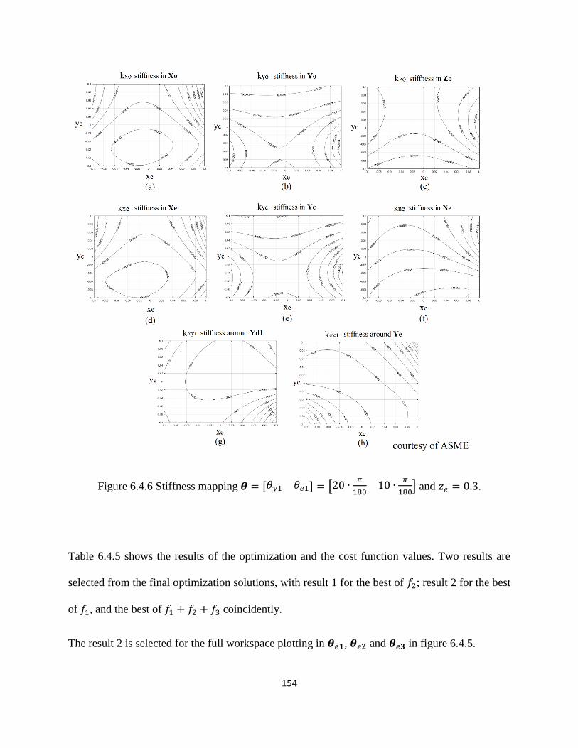
154

Figure 6.4.6 Stiffness mapping 𝜽 = [𝜃𝑦1 𝜃𝑒1] = [20 ∙𝜋

18010 ∙

𝜋

180] and 𝑧𝑒 = 0.3.

Table 6.4.5 shows the results of the optimization and the cost function values. Two results are

selected from the final optimization solutions, with result 1 for the best of 𝑓2; result 2 for the best

of 𝑓1, and the best of 𝑓1 + 𝑓2 + 𝑓3 coincidently.

The result 2 is selected for the full workspace plotting in 𝜽𝒆𝟏, 𝜽𝒆𝟐 and 𝜽𝒆𝟑 in figure 6.4.5.

155

With the diagonal of 𝑲𝒐 and 𝑲𝒆, one gets eight indexes for stiffness, such as 𝑘𝑥𝑜, 𝑘𝑦𝑜, 𝑘𝑧𝑜 which

indicate the translational stiffness in 𝑿𝒐, 𝒀𝒐, 𝒁𝒐 (figure 6.4.6. (a) (b) (c)); 𝑘𝑥𝑒, 𝑘𝑦𝑒 , 𝑘𝑛𝑒 which

indicate translational stiffness in 𝑿𝒆, 𝒀𝒆, 𝑵𝒆 (figure 6.4.6. (d) (e) (f)); and 𝑘𝑤𝑦1, 𝑘𝑤𝑒1 which

indicate the rotational stiffness around 𝒀𝒅𝟏, 𝒀𝒆 (figure 6.4.6. (g) (h)).

6.4.4 Applications

Since the 3T2R parallel manipulator has 5-DOF and lie-flat (deployable) feature, it may find

applications where the structure needs to be folded. When compared to other deployable

mechanisms, this manipulator has higher DOF than designs in [28] [29] [122] while it is different

from a deployable stage [22].

In automobile manufacturing applications, the manipulator could work under the vehicle bodies

for drilling, laser cutting or material spraying tasks, when finished it lies flat to let the vehicle

passes over it until next vehicle moves over it. It could rise again and work under the vehicle body.

Similarly, it could work on the vehicle bodies from top or sides.

It may also find applications for maintenance or power charging of various types of vehicles in the

field. For instance, it could work under the drones, rovers or walking robots that stop over it, then

it extends its 5-DOF moving platform to reach the area on the bottoms of these vehicles. Just like

the solar trackers with lie-flat features which could supply power to this 5-DOF manipulator, they

both can lie flat when destructive storms strike. This feature allows the structure to lie close to

floor as to protect the structure from being destroyed in strong storms. Besides, it could also serve

as a signal receiver stand.

156

When less than 5 DOFs are needed, the redundant mobilities could be adjusted for higher stiffness

in demanded mobilities.

Whatever the applications, the manipulator could lie-flat close to the surface it is mounted on, to

give space or to protect itself.


A 5-DOF 3T2R parallel manipulator with each limb in two perpendicular planes is design from

synthesis method based on motion sets intersection theory and disseminated Chebychev-Grübler-

Kutzbach formula. The link interference detection is checked by boundary offset method

considering the width of the links. Multi-objective design optimization has been practiced.

Stiffness based on both global coordinate and platform coordinate are calculated and plotted for

the loading analysis of the moving platform. Potential applications of the manipulator both indoor

and outdoor have been discussed.


A 5-DOF parallel manipulator and a 6-DOF parallel manipulator are designed that have deployable

function. The 6-DOF manipulator has full mobilities and is designed with three identical 6-DOF

limbs, while the 5-DOF manipulator with non-identical limbs in three mobile vertical planes is

designed based on intersection of motion sets and disseminated G-K formula. The method could

be adopted to develop more high-DOF deployable manipulators with limbs in mobile vertical

planes. The actual DOF is verified by Jacobian matrix.

157

The 6-DOF manipulator interference is checked with pentagon identification, and the Point-line

criteria, while the 5-DOF manipulator interference is checked with link boundary offset method.

The link boundary offset method would be more generally applicable for interference

identification in parallel layers.

Jacobian matrix is modified for translational or rotational stiffness evaluation in any direction.

(example in 3-[(2-RR)UU])

158

Chapter 7 Dissertation Conclusion and Outlook

7.1 Conclusion of Research

Parallel manipulators generally have the advantages of high stiffness and precision compared to

serial manipulators, however their workspaces are limited. The workspace may be further

compromised when additional design requirements set constraints to the design.

Dynamic balancing and deployable feature are significant for manipulators in applications of

precise manufacturing and outdoor solar tracking. The dynamically balanced manipulators contain

additional balancing components, thus the link interference needs to be avoided and its energy

consumption needs to be minimized. The deployable feature in non-configurable platform parallel

manipulator is still rare and needs more research.

When designing dynamically balanced manipulators and deployable manipulators of high DOF

(spatial mobilities greater than three), the link to link interference needs to be checked and avoided.

The parallel manipulators with limbs in fixed or mobile vertical planes have the properties that

provide solutions for dynamic balancing, deployable feature and interference avoidance. Novel

design principles and evaluation methods are discussed. The design of parallel manipulators

follows the process of task, design/evaluation and optimization.

In chapter 4, dynamically balanced planar 2-DOF, 3-DOF and spatial 2R1T 3-DOF machines are

developed. The limbs are balanced in horizontal plane (planar manipulator) or fixed vertical planes

(2R1T manipulator) at revolute joints. The middle joint angles are reversed to avoid link to link

interference. The structural adaption and motion planning are employed for optimal energy

159

consumption results in the 2R1T 3-DOF spatial manipulator. By comparison of the optimization

results, the combination of two approaches works better than structural adaption alone. The (2-

RR)R or (2-RR)R planar manipulator has two base joints capable of relocation (four optimization

variables on structure). The 3-RRS spatial manipulator has three base joints capable of relocation

(three optimization variables on structure). The adjustable variables are offered by kinematic

redundancy. The 3-DOF balanced planar manipulator and 3-DOF spatial balanced manipulator

can be combined to make a 6-DOF balanced manipulator. The combination yields a 6-DOF

dynamically balanced machine with five adaptive base joints (seven optimization variables on

structure) for optimization opportunities.

In chapter 5, two members of the 2R1T 3-DOF P*U* parallel manipulator family, 3-PRS and 3-

RPS, are re-designed with deployable function which is useful for storm protection of outdoor

working robots. For a useful but redundant motion (translation in z axis), a minimum height

algorithm is developed to rapidly calculate eligible workspace. Jacobian transformation matrix is

developed to calculate stiffness in any directions. The 2R1T manipulators have limbs in three fixed

vertical planes and are free from interference. The kinematic redundancy in the fixed vertical

planes offers optimization opportunities and wind energy harvesting opportunities.

In chapter 6, the deployable design is expanded to higher-DOF structures. A 6-DOF manipulator

and a 5-DOF manipulator are designed. Their limbs are in mobile vertical planes. This design has

the property of avoiding link interference and large workspace. The parallel actuation in horizontal

plane that moves the vertical planes need interference check. Parallel horizontal layers partially

avoid the interference and several methods are developed for convenient detection.

160

Genetic algorithm is suitable for complex non-linear problem optimization. The design

optimization could be practiced before operation optimization. The design optimization deals with

design parameters. The operation optimization deals with structural adaptive features and (or)

motion planning for optimal performance of a specific task. Both design optimization and

operation optimization can be single-objective or multi-objective. Among the designs from above

chapters where applicable, maximum total workspace, minimum sizes and (or) minimum lie-flat

height are considered as design optimization objective(s), while the minimum energy consumption

for certain trajectories, maximum workspace at certain operation mode, maximum workspace at

certain area, maximum and (or) maximum general stiffness at certain area are considered as

operation optimization objective(s).

7.2 Research Contributions

Novel design principles and evaluation algorithms are developed. The detailed research

contributions are given below.

7.2.1 Dynamic Balanced Various DOF Manipulators

1) The configuration change on original (2-RR)R or (2-RR)R and 3-RRS through middle joint

angles reversal avoids link interference.

2) Spatial 3-RRS manipulator is designed with three force balanced limbs and two moment

balancing flywheels.

161

3) Structural adaption and motion planning are integrated to seek optimization for minimum

energy consumption in a spatial manipulator. (example in 3-RRS)

4) The combination of two balanced interference-free manipulators provides a higher DOF

balanced manipulator of large workspace. The DOF and structural adaption from the two

individual manipulators are combined.

7.2.2 Re-design of 3-PRS and 3-RPS Deployable Manipulators

1) The 3-PRS and 3-RPS are re-designed with deployable function (lie-flat feature).

2) The 3-RPS hybrid energy harvester harvests wind loads on solar panel through leg deformations.

3) Minimum platform height algorithm rapidly checks eligibility of possible pose of workspace

and shortens the optimization time. (example in 3-RPS)

4) Jacobian matrix transformation for stiffness evaluation in any direction. (example in 3-RPS)

7.2.3 Novel Design of 5-DOF and 6-DOF Deployable Manipulators

1) The 6-DOF (2-RR)UU limb is designed. It has large workspace and is deployable which serves

as limbs for deployable 6-DOF 3-[(2-RR)UU] and 5-DOF PRPU/2-[(2-RR)UU].

2) Link interference is avoided as each limb is distributed in a mobile vertical plane and multiple

horizontal layers. Link boundary offset method rapidly detects link interference for links on a same

horizontal layer. (example in PRPU/2-[(2-RR)UU])

3) Jacobian matrix is modified for stiffness evaluation in any direction. (example in 3-[(2-RR)UU])

162

7.3 Future Research

1.a) The 6-DOF dynamically balanced machine combined by (2-RR)R and 3-RRS manipulators

could be optimized for minimal energy consumption with the five relocatable base joins and

motion planning

1.b) The active force compensation may need to be considered for operations when there includes

large amount material addition or removal which may affect the dynamic balancing.

2.a) The piezo chips on the legs of the 3-RPS hybrid harvester can harvest mechanical energy and

sense the deformation as well. Machine learning algorithm needs to be developed to recognize the

loading condition on the solar panel through piezo chips. This could save the sensor cost of the

model and help to promote the hybrid harvesters to the commercial market.

2.b) A family of high DOF deployable can be designed with the design principles given in above

chapters. Thanks to the composition of vertical and horizontal multiple planar linkages, the

possibilities of linkage of a given DOF might be generated with computer program in each plane.

The computing algorithm will need to be developed.

2.c) The family could be further classified to groups of sub-class manipulators where their unique

properties will be analyzed to match certain categories of applications.

7.4 An Outlook of the Clean Powered Robotic Systems

The figure 7.4.1 shows a system of robots.

163

Figure 7.4.1 A robotic system of balanced and deployable manipulators green energy powered.

With the manipulators developed in the previous chapters, one could have an outlook to the future

indoor and outdoor robotic system that run on solar and wind energy.

164

The balanced manipulator is working in the factory that has low noise and vibration, and is energy

saving.

The deployable manipulator is serving the drones and unmanned vehicles which are transporting

parts between factories. The deployable harvesters supply clean energy to the above manipulators.

The deployable manipulators and deployable harvesters can lie flat to protect themselves from

natural disasters.

This robotic system is operating in a green way and working harmoniously with nature.

165

References

[1] Zamalloa, I., Kojcev, R., Hernandez, A., Muguruza, I., Usategui, L., Bilbao, A.,

Mayoral, V., 2017, “Dissecting Robotics - Historical Overview and Future

Perspectives,” ArXiv 2017.

[2] Royakkers, L., and Van Est, R., 2015, “A Literature Review on New Robotics:

Automation from Love to War,” International Journal of Social Robotics, 7(5), pp.

549-570.

[3] Ting, C., Yeo, W., King, Y., Yea Dat, C., Lee, J., and Khaw, W., 2014, “Humanoid

Robot: A Review of the Architecture, Applications and Future Trend,” Research

Journal of Applied Sciences, Engineering and Technology, 7(7), pp. 1364-1369.

[4] Angeles, J., 2007, Fundamentals of Robotic Mechanical Systems: Theory, Methods,

and Algorithms, Springer, New York.

[5] Raibert, M., Blankespoor, K., Nelson, G., Playter, R., 2008, “BigDog, the Rough-

Terrain Quadruped Robot,” IFAC Proceedings Volumes, 41(2), pp. 10822-10825.

[6] Hung, S., Liu, C., Tsai, A., and Lin, T., 2008, “Design and Implementation of an

Intelligent Robotic Fish,” 2008 IEEE Workshop on Advanced Robotics and Its

Social Impacts, Taipei, August 23-25, 2008, pp. 1-5.

[7] Xu, Y., and Wang, H., 2013, “Flying Robot with Undulating Wings,” IFAC

Proceedings Volumes, 46(30), pp. 181-186.

166

[8] Hodgins, J., 2018, “H-Delta: Design and Applications of a Novel 5 Degree of

Freedom Parallel Robot,” Ph.D. dissertation, University of Ontario Institute of

Technology, Oshawa, ON.

[9] Arns, M., 2019, “Novel Reconfigurable Delta Robot Dual-functioning as Adaptive

Landing Gear and Manipulator,” Master thesis, York University, Toronto, ON.

[10] “The Shuttle Remote Manipulator System -- The Canadarm,” accessed 2019,

https://www.ieee.ca/millennium/canadarm/canadarm_technical.html

[11] Gasparetto, A., and Scalera, L., 2019, “A Brief History of Industrial Robotics in the

20th Century,” Advances in Historical Studies, 8(1), pp. 24-35.

[12] Nam, H., Riviere, E., and Verlinden, O., 2016, “Milling Simulations with a 3-DOF

Flexible Planar Robot,” International Journal of Mechanical, Aerospace, Industrial,

Mechatronic and Manufacturing Engineering, 10(9).

[13] Subhashini, P., Raju, N., and Venkata Rao, G., 2014, “Modeling, Simulation and

Analysis of a SCARA Robot for Deburring of Circular Components,” ARPN

Journal of Engineering and Applied Sciences, 9(4), pp. 398-404.

[14] Zhang, D., 2010, Parallel Robotic Machine Tools, Springer, New York.

[15] Hamdoun, O., Baghli, F., and Bakkali, L., 2015, “Inverse Kinematic Modeling of

3RRR Parallel Robot,” 22ème Congrès Français de Mécanique, Lyon, France,

August 24-28.

167

[16] Patel, Y., and George, P., 2012, “Parallel Manipulators Applications-A Survey,”

Modern Mechanical Engineering, 2(3), pp. 57-64.

[17] Küçük, S., 2012, Serial and parallel robot manipulators: Kinematic dynamics,

control and Optimization, IntechOpen.

[18] Stewart, D., 1965, “A Platform with Six Degrees of Freedom,” Proceedings of the

Institution of Mechanical Engineers, 180(1), pp. 371-386.

[19] Qian, S., Zi, B., Shang, W., and Xu, Q., 2018, “A Review on Cable-driven Parallel

Robots,” Chinese Journal of Mechanical Engineering, 31(66).

[20] Mohamed, M., and Gosselin, C., 2005, “Design and Analysis of Kinematically

Redundant Parallel Manipulators with Configurable Platforms,” IEEE Transactions

on Robotics, 21(3), pp. 277-287.

[21] Jin, X., Fang, Y., Qu, H., and Guo, S., 2018, “A Class of Novel 4-DOF and 5-DOF

Generalized Parallel Mechanisms with High Performance,” Mechanism and

Machine Theory, Volume 120, February 2018, pp. 57-72.

[22] Zeng, Q., and Ehmann, K., 2014, “Design of Parallel Hybrid-loop Manipulators

with Kinematotropic Property and Deployability,” Mechanism and Machine

Theory, Volume 71, January 2014, pp. 1-26.

[23] Tian, C., Fang, Y., and Guo, S., 2016, “Structural Synthesis of a Class of 2R2T

Hybrid Mechanisms,” Chinese Journal of Mechanical Engineering, 29(4), pp. 703-

709.

168

[24] Tian, C., Fang, Y., and Ge, Qi., 2017, “Structural Synthesis of Parallel Manipulators

with Coupling Sub-chains,” Mechanism and Machine Theory, 118, December 2017,

pp. 84-99.

[25] Gosselin, C., 2008, “Gravity Compensation, Static Balancing and Dynamic

Balancing of Parallel Mechanisms,” Smart Devices and Machines for Advanced

Manufacturing. Wang, L., and Xi, J., eds., Springer, London.

[26] Yang, Z., and Zhang, D., (under peer-review/revision 2019), “Novel Planar

Balanced Adaptive (2-RR)R Parallel Manipulator,” International Journal of

Robotics and Automation.

[27] Yang, Z., and Zhang, D., (accepted in February 2019), “Energy Optimal Adaption

and Motion Planning of a 3-RRS Balanced Manipulator,” International Journal of


[28] Yang, Z., and Zhang, D., 2017, “Reconfigurable 3-PRS Parallel Solar Tracking

Stand,” Proceedings of the ASME 2017 International Design Engineering Technical

Conferences and Computers and Information in Engineering Conference,

Cleveland, Ohio, USA, August 6-9, 2017, ASME Paper No. DETC2017-67275.

[29] Yang, Z., and Zhang, D., 2018, “Hybrid Harvester 3-RPS Robotic Parallel

Manipulator,” 2018 2nd International Conference on Artificial Intelligence

Applications and Technologies (AIAAT 2018), Shanghai, China, August 8-10,

2018.

169

[30] Yang, Z., and Zhang, D., 2018, “Novel Design of a 3-RRUU 6-DOF Parallel

Manipulator”, 2018 4th International Conference on Mechanical and Aeronautical

Engineering (ICMAE 2018), Bangkok, Thailand, December 13-16, 2018.

[31] Yang, Z., and Zhang, D., 2019, “Novel Design of a 3T2R 5-DOF Parallel

Manipulator”, Proceedings of the ASME 2019 International Design Engineering

Technical Conferences and Computers and Information in Engineering Conference,

Anaheim, CA, USA, August 18-21, 2019, ASME Paper No. IDETC2019-97088.

[32] Yang, T., Liu, A., Shen, H., Hang, L., Luo, Y., and Jin, Q., 2018, Topology Design

of Robot Mechanisms, Springer, Singapore.

[33] Huang, T., Zhao, D., Yin, F., Tian, W., and Chetwynd, D., 2019, “Kinematic

Calibration of a 6-DOF Hybrid Robot by Considering Multicollinearity in the

Identification Jacobian,” Mechanism and Machine Theory, Volume 131, January

2019, pp. 371-384.

[34] Zhang, D., and Wang, L., 2005, “Conceptual Development of an Enhanced Tripod

Mechanism for Machine Tool,” Robotics and Computer-Integrated Manufacturing,

Volume 21, Issues 4-5, pp. 318-327.

[35] Li, J., 2009, “Design of 3-DOF Parallel Manipulators for Micro-motion

Applications,” Master Thesis, University of Ontario Institute of Technology,

Oshawa, ON.

[36] Gogu, G., 2005, “Mobility of Mechanisms: A Critical Review,” Mechanism and

Machine Theory, 40(9), pp. 1068-1097.

170

[37] Gogu, G., 2005, “Chebychev–Grübler–Kutzbach's Criterion for Mobility

Calculation of Multi-loop Mechanisms Revisited via Theory of Linear

Transformations,” European Journal of Mechanics - A/Solids, 24(3), pp. 427-441.

[38] Zhao, J., Zhou, K., and Feng, Z., 2004, “A Theory of Degrees of Freedom for

Mechanisms,” Mechanism and Machine Theory, 39(6), pp. 621-643.

[39] Huang, Z., Liu, J., and Li, Y., 2011, “150-year Unified Mobility Formula Issue,”

Journal of Yanshan University, 35(1), pp. 1-14.

[40] Angeles, J., and Gosselin, C., 1988, “Determination Du Degre De Liberte Des

Chaines Cinematique,” Transactions of the Canadian Society for Mechanical

Engineering, Volume 12, No. 4, pp. 219-226.

[41] Gosselin, C., 1990, “Stiffness Mapping for Parallel Manipulators,” IEEE

Transactions on Robotics and Automation, Volume 6, Issue 3, pp. 377-382.

[42] Yang, D., Xiong, J., and Yang, X., 2008, “A Simple Method to Calculate Mobility

with Jacobian,” Mechanism and Machine Theory, 43(9), pp. 1175-1185.

[43] Qu, S., Li, R., and Bai, S., 2017, “Type Synthesis of 2T1R Decoupled Parallel

Mechanisms Based on Lie Groups and Screw Theory,” Mathematical Problems in

Engineering, Volume 2017, pp. 1-11.

[44] Gosselin, C., 1988, “Kinematic Analysis, Optimization and Programming of Parallel

Robotic Manipulators,” Ph.D. dissertation, McGill University, Montreal, QC.

171

[45] Tsai, L., 2000, Mechanism Design: Enumeration of Kinematic Structures According

to Function, CRC Press.

[46] Wang, X., Baron, L., and Cloutier, G., 2008, “Topology of Serial and Parallel

Manipulators and Topological Diagrams,” Mechanism and Machine Theory, 43(6),

pp. 754-770.

[47] Gao, F., Yang, J., and Ge, Q., 2011, “Type Synthesis of Parallel Mechanisms Having

the Second Class GF Sets and Two Dimensional Rotations,” Journal of Mechanisms

and Robotics Transactions of the ASME, 3(1).

[48] Landure, L., and Gosselin, C., 2018, “Kinematic Analysis of a Novel Kinematically

Redundant Spherical Parallel Manipulator,” Journal of Mechanisms and Robotics

Transactions of the ASME, 10(2).

[49] Li, Q., Chai, X., and Chen, Q., 2017, “Review on 2R1T 3-DOF Parallel

Mechanisms,” Chinese Science Bulletin, Volume 62, pp. 1507-1519.

[50] Siciliano, B., 1999, “The Tricept Robot: Inverse Kinematics, Manipulability

Analysis and Closed-loop Direct Kinematics Algorithm,” Robotica, Volume 17, pp.

437-445.

[51] Chen, X., Liu, X., Xie, F., and Su, Tao., 2014, “A Comparison Study on

Motion/Force Transmissibility of Two Typical 3-DOF Parallel Manipulators: The

Sprint Z3 and A3 Tool Heads,” International Journal of Advanced Robotic Systems,

pp. 1-10.

172

[52] Zhang, D., and Gosselin, C., 2002, “Kinetostatic Analysis and Design Optimization

of the Tricept Machine Tool Family,” Journal of Manufacturing Science and

Engineering, Transactions of the ASME, 124(3).

[53] Gao, Z., and Zhang, D., 2014, “Performance Analysis, Mapping, and Multiobjective

Optimization of a Hybrid Robotic Machine Tool,” IEEE Transactions on Industrial

Electronics, Volume 62, Issue 1, pp. 423-433.

[54] Bi, Z., and Jin, Y., 2011, “Kinematic Modeling of Exechon Parallel Kinematic

Machine,” Robotics and Computer-Integrated Manufacturing, 27(1), pp. 186-193.

[55] Mejia, L., Simas, H., and Martins. D., 2015, “Force Capability in General 3 DoF

Planar Mechanisms,” Mechanism and Machine Theory, Volume 91, pp. 120-134.

[56] Qin, Y., Hai, Y., Zhou, C., and Cao, Y., 2015, “Structural Synthesis of 3T2R Five-

Degree-of-Freedom (DoF) Hybrid Mechanism,” The 5th Annual IEEE International

Conference on Cyber Technology in Automation, Control and Intelligent Systems,

Shenyang, China, June 8-12, 2015, pp. 65-70.

[57] Lu, Y., and Dai, Z., 2016, “Dynamics Model of Redundant Hybrid Manipulators

Connected in Series by Three or More Different Parallel Manipulators with Linear

Active Legs,” Mechanism and Machine Theory, Volume 103, pp. 222-235.

[58] Chablat, D., Wenger, P., and Angeles, J., 1998, “The Kinematic Design of a 3-dof

Hybrid Manipulator,” Integrated Design and Manufacturing in Mechanical

Engineering, Compiègne, France, pp.1-8.

173

[59] Yeshmukhametov, A., Kalimoldayev, M., Mamyrbayev, O., and Amirgaliev, Y.,

2017, “Design and Kinematics of Serial/Parallel Hybrid Robot,” 2017 3rd

International Conference on Control, Automation and Robotics (ICCAR), Nagoya,

Japan, April 24-26, 2017, pp. 162-165.

[60] Lin, R., Guo, W., and Gao, F., 2016, “Type Synthesis of a Family of Novel Four,

Five, and Six Degrees-of-Freedom Sea Lion Ball Mechanisms with Three Limbs,”

Journal of Mechanisms and Robotics Transactions of the ASME, 8(2).

[61] Behi, F., 1988, “Kinematic Analysis for a Six-Degree-of-Freedom 3-PRPS Parallel

Mechanism,” IEEE Journal on Robotics and Automation, 4(5), pp. 561-565.

[62] Simaan, N., Glozman, D., and Shoham, M., 1998, “Design Considerations of New

Six Degrees-of-Freedom Parallel Robots,” Proceedings of 1998 IEEE International

Conference on Robotics and Automation, Leuven, Belgium, May 1998, pp. 1327-

1333.

[63] Alizade, R., Tagiyev, N., and Duffy, J., 1994, “A Forward and Reverse

Displacement Analysis of a 6-DOF In-Parallel Manipulator,” Mechanism and

Machine Theory, Volume 29, Issue 1, pp. 115-124.

[64] Kim, J., Park, F. C., Ryu, S. J., Kim, J., Hwang, J. C., Park, C., and Iurascu, C. C.,

2001, “Design and Analysis of a Redundantly Actuated Parallel Mechanism for

Rapid Machining,” IEEE Transactions on Robotics and Automation, 17(4), pp. 423-

434.

174

[65] Chen, C., Gayral, T., Caro, S., Chablat, D., Moroz, G., and Abeywardena, S., 2012,

“A Six Degree of Freedom Epicyclic-Parallel Manipulator,” Journal of Mechanisms

and Robotics, Transactions of the ASME, 4(4).

[66] Tahmasebi, F., and Tsai, L., 1992, “Jacobian and Stiffness Analysis of a Novel Class

of Six-DOF Parallel Mini Manipulators”, 22nd ASME Biennial Mechanisms

Conference, Scottsdale, AZ, September 1992.

[67] Li, W., and Angeles, J., 2017, “A Novel Three-loop Parallel Robot with Full

Mobility: Kinematics, Singularity, Workspace, and Dexterity Analysis,” Journal of

Mechanisms and Robotics, Transactions of the ASME, 9(5).

[68] Monsarrat, B., and Gosselin, C., 2003, “Workspace Analysis and Optimal Design of

a 3-Leg 6-DOF Parallel Platform Mechanism,” IEEE Transactions on Robotics and

Automation, 19(6), pp. 954-966.

[69] Yang, G., Chen, I., Chen, W., and Lin, W., 2004, “Kinematic Design of a Six-DOF

Parallel-Kinematics Machine with Decoupled-Motion Architecture,” IEEE

Transactions on Robotics and Automation, 20(5), pp. 876-884.

[70] Lee, S., and Kim, S., “Kinematic feature analysis of parallel manipulator systems,”

Proceedings of IEEE/RSJ International Conference on Intelligent Robots and

Systems (IROS'94), Munich, Germany, 1994, Volume 2, pp. 1421-1428.

[71] Guo, S., and Qu, H., 2016, Structural Synthesis of Redundant Parallel Robots and

Its Applications, Science Press China, Beijing, China.

175

[72] Luces, M., and Mills, J., and Benhabib, B., 2017, “A Review of Redundant Parallel

Kinematic Mechanisms,” Journal of Intelligent & Robotic Systems, 86(2), pp. 175-

198.

[73] Gosselin, C., & Schreiber, L., 2018, “Redundancy in Parallel Mechanisms: A

Review,” Applied Mechanics Reviews, Transactions of the ASME, 70(1).

[74] Fahimi, F., 2009, Autonomous Robots: Modeling, Path Planning, and Control.

Springer, New York.

[75] Gosselin, C., Laliberte, T., and Veillette, Audrey., 2015, “Singularity-Free

Kinematically Redundant Planar Parallel Mechanisms with Unlimited Rotational

Capability,” IEEE Transactions on Robotics, 31(2), pp. 457-467.

[76] Santos, J., Rocha, D., and Silva, M., 2014, “Performance Evaluation of

Kinematically Redundant Planar Parallel Manipulators,” ABCM Symposium Series

in Mechatronics, Volume 6, pp. 391-401.

[77] Varalakshmi, K., and Srinivas, J., 2014, “Optimized Configurations of

Kinematically Redundant Planar Parallel Manipulator following a Desired

Trajectory,” Procedia Technology, Volume 14, pp. 133-140.

[78] Maraje, S., Nurahmi, L., and Caro, S., 2016, “Operation Modes Comparison of a

Reconfigurable 3-PRS Parallel Manipulator Based on Kinematic Performance,”

ASME 2016 International Design Engineering Technical Conferences and

Computers and Information in Engineering Conference, Charlotte, North Carolina,

USA, August 21-24, 2016, ASME Paper No. DETC2016-59804.

176

[79] Kotlarski, J., Abdellatif, H., and Heimann, B., 2008, “Improving the Pose Accuracy

of a Planar 3RRR Parallel Manipulator Using Kinematic Redundancy and

Optimized Switching Patterns,” 2008 IEEE International Conference on Robotics

and Automation, Pasadena, CA, USA, May 19-23, 2008, pp. 3863-3868.

[80] Liu, H., Huang, T., Kecskeméthy, A., and Chetwynd, D., 2015, “Force / Motion /

Stiffness Transmissibility Analyses of Redundantly Actuated and Overconstrained

Parallel Manipulators,” The 14th IFToMM World Congress, Taipei, Taiwan,

October 25-30, 2015.

[81] Mueller, A., 2008, “Redundant Actuation of Parallel Manipulators,” Parallel

Manipulators, Towards New Applications. Wu, P., eds., I-Tech Education and

Publishing, Vienna, Austria, pp. 87-108.

[82] Cheng, H., Liu, G., Yiu, Y., Xiong, Z., and Li, Z., 2001, “Advantages and Dynamics

of Parallel Manipulators with Redundant Actuation,” Proceedings of the 2001

IEEE/RSJ International Conference on Intelligent Robots and Systems, Maui,

Hawaii, USA, Oct 29-Nov 03, 2001, pp. 171-176.

[83] Wu, J., Chen, X., Li, T., and Wang, L., 2013, “Optimal Design of a 2-DOF Parallel

Manipulator with Actuation Redundancy Considering Kinematics and Natural

Frequency,” Robotics and Computer-Integrated Manufacturing, 29(1), pp. 80-85.

[84] Arakelian, V., 2015, “Optimum Shaking Force Balancing of Planar 3-RRR Parallel

Manipulators by Means of an Adaptive Counterweight System,” Journal of Robotics

and Mechanical Engineering Research, 1(2), pp. 36-41.

177

[85] Dresig, H., and Dien, N., 2011, “Complete Shaking Force and Shaking Moment

Balancing of Mechanisms Using a Moving Rigid Body,” TECHNISCHE

MECHANIK, 31(2), pp. 121-131.

[86] Coppola, G., 2014, “Advances in Parallel Robotics for Flexible and Reconfigurable

Manufacturing,” Ph.D. dissertation, University of Ontario Institute of Technology,

Oshawa, ON.

[87] Coppola, G., Zhang, D., and Liu, K., 2014, “A New Class of Adaptive Parallel

Robots,” Journal of Mechanisms and Robotics, Transactions of the ASME, 6(4).

[88] Bi, Z., Lin, Y., and Zhang, W., 2010, “The General Architecture of Adaptive

Robotic Systems for Manufacturing Applications,” Robotics and Computer-

Integrated Manufacturing, 26(5), pp. 461-470.

[89] Zhang, T., Zhang, W., and Gupta, M., 2018, “An Underactuated Self-

Reconfigurable Robot and The Reconfiguration Evolution,” Mechanism and

Machine Theory, Volume 124, pp. 248-258.

[90] Li, J., Wang, J., Chou, W., Zhang, Y., Wang, T., and Zhang, Q., 2001, “Inverse

Kinematics and Dynamics of the 3-RRS Parallel Platform,” Proceeding of the 2001

IEEE International Conference on Robotics & Automation, Seoul, Korea, May 21-

26, 2001, pp. 2506-2511.

[91] Li, Y., and Xu, Q., 2004, “Kinematics and Stiffness Analysis for a General 3-PRS

Spatial Parallel Mechanism”, ROMANSY Conference 2004, Montreal, Canada,

June 14-18, 2004.

178

[92] Babu, S., Raju, V., and Ramji, K., 2013, “Design for Optimal Performance of 3-RPS

Parallel Manipulator Using Evolutionary Algorithms”, Transactions of the Canadian

Society for Mechanical Engineering, Vol. 37, No. 2, pp. 135-160.

[93] “D’Alembert’s Principle,” accessed 2016, https://en.wikipedia.org.

[94] Rahmat Abadi, B., Taghvaei, S., and Vatankhah, R., 2016, “Optimal Motion

Planning of a Planar Parallel Manipulator with Kinematically Redundant Degrees

of Freedom,” Transactions of Canadian Society for Mechanical Engineering, 40(3),

pp. 383-397.

[95] “MathWorks Documentations: Mechanical Dynamics,” accessed 2017,

https://www.mathworks.com/help/physmod/sm/mech/ug/mechanical-

dynamics.html.

[96] Sun, Z., Zhang, B., Cheng, L., and Zhang, W., 2011 “Application of the Redundant

Servomotor Approach to Design of Path Generator with Dynamic Performance

Improvement,” Mechanism and Machine Theory, 46 (11), pp. 1784–1795.

[97] Hu, J., Zhang, X., and Zhan, J., 2008, “Trajectory Planning of a Novel 2-DoF High-

Speed Planar Parallel Manipulator,” Intelligent Robotics and Applications. ICIRA

2008. Lecture Notes in Computer Science. Xiong, C., Huang, Y., Xiong, Y., and

Liu, H., eds, Springer, Berlin.

[98] Abdellatif, H., and Heimann, B., 2005, “Adapted Time-Optimal Trajectory Planning

for Parallel Manipulators with Full Dynamic Modelling,” Proceedings of the 2005

179

IEEE International Conference on Robotics and Automation, Barcelona, Spain,

April 2005, pp. 411-416.

[99] Lorenz, M., Paris, J., Haschke, T., Schöler, F., Hüsing, M., and Corves, B., 2017,

“A Study on Efficient Motion Design for Redundantly Actuated Parallel Kinematic

Manipulators,” 2017 IEEE/RSJ International Conference on Intelligent Robots and

Systems (IROS), Vancouver, BC, Canada, September 24-28, 2017, pp. 5638-5645.

[100] Mei, Y., Lu, Y., Hu, Y., and Lee, C., 2004, “Energy-efficient Motion Planning for

Mobile Robots,” Proceedings of the 2004 IEEE International Conference on

Robotics and Automation, New Orleans, LA, USA, April 2004, pp. 4344-4349.

[101] “Polynomial Interpolation,” accessed 2017, http://wikipedia.org.

[102] “Genetic Algorithm: Find Global Minima for Highly Nonlinear Problems,” accessed

2016, https://www.mathworks.com/discovery/genetic-algorithm.html.

[103] Chong, E., and Zak, S., 2013, An Introduction to Optimization (Fourth Edition),

John Wiley & Sons, Canada.

[104] “Multi-objective Optimization,” accessed 2016, https://en.wikipedia.org.

[105] Zhang, D., and Wei, B., 2016, Dynamic Balancing of Mechanisms and Synthesizing

of Parallel Robots, Springer International Publishing.

[106] Wei, B., 2016, “Performance Improvement for Robotic Mechanisms by: Synthesis

Design, Dynamic Balancing and Adaptive Control Techniques,” Ph.D. dissertation,

University of Ontario Institute of Technology, Oshawa, ON.

180

[107] Zhang, D., and Wei, B., 2015, “Dynamic Balancing of Parallel Manipulators

Through Reconfiguration,” Proceedings of the ASME 2015 Dynamic Systems and

Control Conference, Columbus, Ohio, USA, October 28-30, 2015, ASME Paper No.

DSCC2015-9669.

[108] Zhang, D., and Wei, B., 2017, “Dynamic Balancing of Robotic Mechanisms via

Reconfiguration and Integration Design,” International Journal of Robotics and

Automation, 32(6), pp. 551-559.

[109] Arakelian, V., and Smith, M., 2005, “Shaking Force and Shaking Moment

Balancing of Mechanisms: A Historical Review with New Examples,” Journal of

Mechanical Design, Transactions of the ASME, 127(2), pp. 334-339.

[110] Ricard, R., and Gosselin, C., 2000, “On the Development of Reactionless Parallel

Manipulators,” Proceedings of DETC’00 ASME 2000 Design Engineering


Baltimore, Maryland, September 10-13, 2000, ASME Paper No.

DETC2000/MECH-14098.

[111] Wu, Y., and Gosselin, C., 2005, “Design of Reactionless 3-DOF and 6-DOF Parallel

Manipulators Using Parallelepiped Mechanisms,” IEEE Transactions on Robotics,

21(5), pp. 821-833.

[112] Coppola, G., Zhang, D., Liu, K., and Gao, Z., 2013, “Design of Parallel Mechanisms

for Flexible Manufacturing with Reconfigurable Dynamics,” Journal of Mechanical

Design, Transactions of the ASME, 135(7).

181

[113] Ouyang, P., and Zhang, W., 2005, “Force Balancing of Robotic Mechanisms Based

on Adjustment of Kinematic Parameters,” Journal of Mechanical Design,

Transactions of the ASME, 127(3), pp. 433-440.

[114] Buganza, A., and Acevedo, M., 2011, “Dynamic Balancing of a 2-DOF 2 RR Planar

Parallel Manipulator by Optimization,” 13th World Congress in Mechanism and

Machine Science, Guanajuato, Mexico, June 19-25, 2011.

[115] Wang, K., Luo, M., Mei, T., Zhao, J., and Cao, Y., 2013, “Dynamics Analysis of a

Three-DOF Planar Serial-Parallel Mechanism for Active Dynamic Balancing with

Respect to a Given Trajectory,” International Journal of Advanced Robotic Systems,

Volume 10.

[116] Wijk, V., and Herder, J., 2010, “Active Dynamic Balancing Unit for Controlled

Shaking Force and Shaking Moment Balancing,” Proceedings of the ASME Design

Engineering Technical Conference, Montreal, Quebec, Canada, Aug. 15-18, 2010,

ASME Paper No. DETC2010-28423.

[117] Arakelian, V., and Smith, M., 2008, “Design of Planar 3-DOF 3-RRR Reactionless

Parallel Manipulators,” Mechatronics, 18(10), pp. 601-606.

[118] Wijk, V., and Herder, J., 2008, “Dynamic Balancing of Mechanisms by using an

Actively Driven Counter-Rotary Counter-Mass for Low Mass and Low Inertia,”

Proceedings of the Second International Workshop on Fundamental Issues and

Future Research Directions for Parallel Mechanisms and Manipulators, Montpellier,

France, September 21-22, 2008, pp. 241-251.

182

[119] “Tropical Storm Risk (TSR),” accessed 2017, http://www.tropicalstormrisk.com.

[120] “Solar Field in Ontario Sees Damage Following Winter Storm,” last modified

November 26, 2016, accessed 2017, http://13wham.com/news/top-stories/solar-

field-in-ontario-sees-damage-following-winter-storm.

[121] Thurston, C., 2015, “Ensuring Your Solar Array Doesn't Get Caught in the Wind,”

Renewable Energy World, 18(4).

[122] Zhao, D., Zhao, J., and Yan, Z., 2016, “Planar Deployable Linkage and Its

Application in Overconstrained Lift Mechanism,” Journal of Mechanisms and

Robotics, Transactions of the ASME, 8(2).

[123] Liu, X., Wang, J., and Pritschow, G., 2005, “A New Family of Spatial 3-DoF Fully-

Parallel Manipulators with High Rotational Capability,” Mechanism and Machine

Theory, Volume 40, Issue 4, 2005, Pages 475-494.

[124] Liu, X., Wang, J., and Kim, J., 2009, “A New Family of Spatial 3-DOF Parallel

Manipulators with Two Translational and One Rotational DOFs,” Robotica, 27(2),

pp. 241-247.

[125] Li, B., Yu, H., Deng, Z., Yang, X., and Hu, H., 2010, “Stiffness Modeling of a

Family of 6DoF Parallel Mechanisms with Three Limbs Based on Screw Theory,”

Journal of Mechanical Science and Technology, 24(1), pp. 373-382.

[126] Merlet, J., 1992, “Geometrical Determination of the Workspace of a Constrained

Parallel Manipulator”, Advances in Robot Kinematics, Ferrare, September 7-9,

1992, pp. 326-329.

183

[127] Zaidie Abdul Majid, M., Huang, Z., and Yao, Y., 1999, “Workspace Analysis of a

New Parallel Manipulator,” Transactions of NAMRI/SME, Volume XXVII, 1999,

pp. 305-310.

[128] Merlet, J., Gosselin, C., and Mouly, N., 1998, “Workspaces of Planar Parallel

Manipulators,” Mechanism and Machine Theory, Volume 33, Issues 1-2, pp. 7-20.

[129] Lumelsky, V., 1985, “On Fast Computation of Distance Between Line Segments,”

Information Processing Letters, Volume 21, Issue 2, pp. 55-61.

[130] Merlet, J., 1995, “Determination of the Orientation Workspace of Parallel

Manipulators,” Journal of Intelligent and Robotic Systems, Volume 13, Issue 2, pp.

143-160.

[131] Zhang, F., Zhu, Y., Furukawa, T., and Song, W., 2015, “Kinematic Analysis of a

Partially Decoupled 3-DOF Parallel Wrist,” Journal of Robotics, 2015(9), pp. 1-9.

[132] Tao, Z., and An, Q., 2013, “Interference Analysis and Workspace Optimization of

3-RRR Spherical Parallel Mechanism,” Mechanism and Machine Theory, Volume

69, pp. 62-72.

[133] Sen, D., and Joshi, V., 2004, “Issues in Geometric Synthesis of Mechanisms,”

Mechanism and Machine Theory, Volume 39, Issue 12, pp. 1321-1330.

[134] Ling, Z., and Chase, T., 1996, “A Priori Geometric Design of an Interference Free

Complex Planar Mechanism,” Mechanism and Machine Theory, Volume 31, Issue

4, pp. 513-524.

184

[135] Schreiber, L., and Gosselin, C., 2017, “Passively Driven Redundant Spherical Joint

with Very Large Range of Motion,” Journal of Mechanisms and Robotics,

Transactions of the ASME, 9(3).

[136] Talaba, D., 2012, “The Angular Capacity of Spherical Joints Used in Mechanisms

with Closed Loops and Multiple Degrees of Freedom,” Robotics and Computer-

Integrated Manufacturing, Volume 28, Issue 5.

[137] Hudgens, J., and Arai, T., 1993, “Planning Link-interference-free Trajectories for a

Parallel Link Manipulator,” Proceedings of IECON '93 - 19th Annual Conference

of IEEE Industrial Electronics, Maui, Hawaii, USA, Nov. 15-19, 1993, pp. 1506-

1511.

[138] Alici, G., and Shirinzadeh, B., 2004, “Optimum Dynamic Balancing of Planar

Parallel Manipulators,” Proceedings of the 2004 IEEE International Conference on

Robotics and Automation, New Orleans, LA, USA, April 26-May 1, 2004, pp. 4527-

4532.

[139] Luo, L., Yuan, C., Yan, R., Yuan, Q., Wu, J., Shin, K., and Han, C., 2015,

“Trajectory Planning for Energy Minimization of Industry Robotic Manipulators

Using the Lagrange Interpolation Method,” International Journal of Precision

Engineering and Manufacturing, 16(5), pp. 911-917.

[140] Gregory, J., Olivares, A., and Staffetti, E., 2013, “Energy-Optimal Trajectory

Planning for Planar Underactuated RR Robot Manipulators in the Absence of

Gravity,” Abstract and Applied Analysis, Volume 2013.

185

[141] “Back EMF in a Motor,” accessed 2016, https://www.researchgate.net.

[142] Gu, S., 2007, Fundamentals of Electrical Machines and Drives, 4th Edition, China

Machine Press, Beijing.

[143] “Rotation Matrix,” accessed 2017, http://en.wikipedia.org.

[144] Tudorache, T., and Kreindler, L., 2010, “Design of a Solar Tracker System for PV

Power Plants,” Acta Polytechnica Hungarica, Vol. 7, No. 1, pp. 23-39.

[145] “How to Create a Solar Panel that Tracks the Sun,” accessed 2016, https://www.pc-

control.co.uk/howto_tracksun.htm.

[146] Gnanarathinam, D., Sundaramurthy, S., and Wahi, A., 2015, “Design and

Implementation of a Dual Axis Solar Tracking System,” International Journal for

Research in Applied Science and Engineering Technology, Vol. 3, Issue X.

[147] Cammarata, A., 2014, “Optimized Design of a Large-workspace 2-DOF Parallel

Robot for Solar Tracking Systems,” Mechanism and Machine Theory, Volume 83,

pp. 175-186.

[148] “Design of Multiaxial Parallel Kinematic Machines with High Dynamic

Capabilities,” accessed 2016, http://www.ehu.eus/compmech/research-

2/projects/design-of-multiaxial-parallel-kinematic-machines-with-high-dynamic-

capabilities-dynamech/.

186

[149] Shyam, R., and Ghosal, A., 2015, “Three-Degree-of-Freedom Parallel Manipulator

to Track the Sun for Concentrated Solar Power Systems,” Chinese Journal of

Mechanical Engineering, 28(4), pp. 793-800.

[150] Murphy, L., 1980, “Wind Loading on Tracking and Field Mounted Solar

Collectors,” Solar Energy Research Institute, United States. Doi: 10.2172/6889663.

[151] Bhadurl, S., and Murphy, L., 1985, “Wind Loading on Solar Collectors,” Solar

Energy Research Institute, United States.

[152] Liu, C., 2012, Foundations of MEMS, Second Edition, Prentice Hall, NJ.

[153] Sirohi, J., and Mahadik, R., 2011, “Piezoelectric Wind Energy Harvester for Low-

Power Sensors,” Journal of Intelligent Material Systems and Structures, 22(18) pp.

2215-2228.

[154] Tao, J., Viet, N., Carpinteri, A., and Wang, Q., 2017, “Energy harvesting from Wind

by A Piezoelectric Harvester,” Engineering Structures, 133(15), pp. 74-80.

[155] Sirohi, J., and Mahadik, R., 2012, “Harvesting Wind Energy Using a Galloping

Piezoelectric Beam,” Journal of Vibration and Acoustics, Transactions of ASME,

134(1).

[156] Yuan, G., and Wang, D., 2017, “A Piezoelectric Six-DOF Vibration Energy

Harvester Based on Parallel Mechanism: Dynamic Modeling, Simulation, and

Experiment,” Smart Materials and Structures, 26(3).

[157] Linear Table Alpha 15-B-155, HSB alpha Release: 12.12.2016.

187

[158] Linear Actuators: DLA Series and Accessories, 50 mm to 300 mm stroke 1000 N,

Transmotec 2018.

[159] Budynas, R., and Nisbett, J., 2008, Shigley’s Mechanical Engineering Design, Ninth

Edition, McGraw-Hill, New York, pp.1013.

[160] “Material: Lead Zirconate Titanate (PZT),” accessed 2018,

https://www.memsnet.org/material/leadzirconatetitanatepzt/.

[161] Campos, L., Bourbonnais, F., Boney, I., and Bigras, P., 2010, “Development of a

Five-Bar Parallel Robot with Large Workspace,” Proceedings of the ASME 2010

International Design Engineering Technical Conferences and Computers and

Information in Engineering Conference, Montreal, Quebec, Canada, August 15-18,

2010, ASME Paper No. DETC2010-28962, pp. 917-922.

[162] Ferrari, D., and Giberti, H., 2014, “A Genetic Algorithm Approach to the Kinematic

Synthesis of a 6-DOF Parallel Manipulator,” 2014 IEEE Conference on Control

Applications (CCA) Part of 2014 IEEE Multi-conference on Systems and Control,

Antibes, France, October 8-10, 2014.

[163] Ayob, M., Zakaria, W., Jalani, J., and Tomari, M., 2015, “Inverse Kinematics

Analysis of a 5-axis RV-2AJ Robot Manipulator,” ARPN Journal of Engineering

and Applied Sciences, Vol. 10, No. 18.

[164] Manjunath, T., 2007, “Kinematic Modelling and Maneuvering of A 5-Axes

Articulated Robot Arm,” International Journal of Mechanical, Aerospace, Industrial,

Mechatronic and Manufacturing Engineering, Vol. 1, No. 4.

188

[165] Masouleh, M., Gosselin, C., and Husty, M., 2011, “Forward Kinematic Problem of

5-RPUR Parallel Mechanisms (3T2R) with Identical Limb Structures,” Mechanisms

and Machine Theory, 46 (7), pp. 945-959.

[166] Amine, S., Tale-Masouleh, M., Caro, S., Wenger, P., and Gosselin, C., 2011,

“Singularity Analysis of 5-DOF Parallel Mechanisms 3T2R Using Grassmann-

Cayley Algebra and Grassmann Line Geometry,” 13th World Congress in

Mechanism and Machine Science, Guanajuato, Mexico, June 19-25, 2011.

[167] DC motors (15W~120W) DKM AC/DC Geared Motor and Gearhead, RAVEO.

189

Appendices

Appendix A: List of Papers during PhD Studies

Journal articles

[26] Yang, Z., and Zhang, D., (under peer-review/revision 2019), “Novel Planar

Balanced (2-RR)R Parallel Manipulator Adaptive for Energy Efficiency,”

International Journal of Robotics and Automation.

[27] Yang, Z., and Zhang, D., (accepted in February 2019), “Energy Optimal Adaption

and Motion Planning of a 3-RRS Balanced Manipulator,” International Journal of


Conference articles

[28] Yang, Z., and Zhang, D., 2017, “Reconfigurable 3-PRS Parallel Solar Tracking

Stand,” Proceedings of the ASME 2017 International Design Engineering Technical

Conferences and Computers and Information in Engineering Conference,

Cleveland, Ohio, USA, August 6-9, 2017, ASME Paper No. DETC2017-67275.

[29] Yang, Z., and Zhang, D., 2018, “Hybrid Harvester 3-RPS Robotic Parallel

Manipulator,” 2018 2nd International Conference on Artificial Intelligence

Applications and Technologies (AIAAT 2018), Shanghai, China, August 8-10,

2018.

190

[30] Yang, Z., and Zhang, D., 2018, “Novel Design of a 3-RRUU 6-DOF Parallel

Manipulator”, 2018 4th International Conference on Mechanical and Aeronautical

Engineering (ICMAE 2018), Bangkok, Thailand, December 13-16, 2018.

[31] Yang, Z., and Zhang, D., 2019, “Novel Design of a 3T2R 5-DOF Parallel

Manipulator”, Proceedings of the ASME 2019 International Design Engineering


Anaheim, CA, USA, August 18-21, 2019, ASME Paper No. IDETC2019-97088.

Note:

Paper [26] has been revised according to peer-review comments and has been resubmitted for peer-

review. Currently it is waiting for decision from the journal.

Paper [27] is a journal paper. It has been accepted for publication and the final paper has been

submitted. Currently it is waiting for publication.

191

Appendix B: Copyright Permission Letters

Permission for article [27].

192


193

Permission for articles [29] and [30].

194


novel design and analysis of parallel robotic …

Documents