nowcasting and data mining storms on weather...
TRANSCRIPT

VA L L I A P PA L A K S H M A N A N
N AT I O N A L S E V E R E S T O R M S L A B O R AT O R Y / U N I V E R S I T Y O F O K L A H O M A
L A K S H M A N @ O U . E D U
AT
T H E C L I M AT E C O R P O R AT I O N
M AY 2 0 1 4
Nowcasting and Data Mining Storms on Weather Radar

Nowcasting and Data Mining
2
Data Mining can answer questions like this: How many days of 2” hail does a location experience? What is the average US population affected by 2” hail every year? Given a climate forecast, what is the expected economic cost of damage?
Can it be used to answer this question? What is the likelihood of rainfall at X given that it rained at Y?
X, Y could be times X, Y could be spatial points
How about these questions? What is the likelihood that a supercell will produce a tornado? What is the likelihood of 2” hail from a squall line? What is the likelihood of a NYC tunnel flooding from a tropical storm?
How are these questions different?

Data Mining in Space and Time
3
Climatology questions Can often treat spatial points as independent or Markov processes Take out the impact of time by accumulating over long time periods
Prediction question What is the likelihood of rainfall at X given that it rained at Y?
X,Y could be times Dynamics, numerical weather prediction models, nowcasting Iterative solutions to handle space-time interaction
X, Y could be spatial points Kriging, “objective analysis” Factor out time by accumulating over long time periods
These are spatio-temporal questions that rely on first detecting storms What is the likelihood that a supercell will produce a tornado? What is the likelihood of 2” hail from a squall line? What is the likelihood of a NYC tunnel flooding from a tropical storm?
Let’s take the harder question first, and then come back to nowcasting

Data Mining Storm Attributes
4
Introduction
Storm Identification
Storm Association
Extracting Storm characteristics
Estimating Motion
Nowcasting
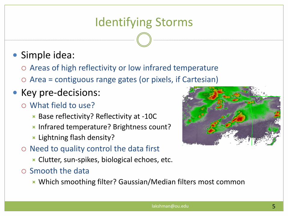
Identifying Storms
5
Simple idea: Areas of high reflectivity or low infrared temperature
Area = contiguous range gates (or pixels, if Cartesian)
Key pre-decisions: What field to use?
Base reflectivity? Reflectivity at -10C
Infrared temperature? Brightness count?
Lightning flash density?
Need to quality control the data first Clutter, sun-spikes, biological echoes, etc.
Smooth the data Which smoothing filter? Gaussian/Median filters most common
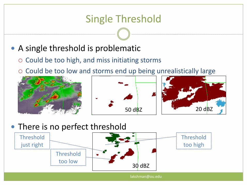
Single Threshold
A single threshold is problematic Could be too high, and miss initiating storms
Could be too low and storms end up being unrealistically large
There is no perfect threshold
20 dBZ 50 dBZ
30 dBZ
Threshold too low
Threshold just right
Threshold too high

Enhanced Watershed
7
Storm = contiguous pixels above t2 that have at least one pixel above t1 t2 = highest value that will allow objects be at least N pixels
Change N to get
multi-scale
30 dBZ 5 px
30 dBZ 10 px
40 dBZ 5 px
40 dBZ 10 px
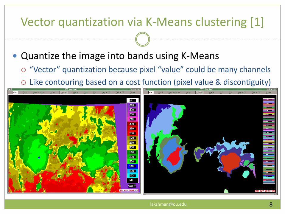
Vector quantization via K-Means clustering [1]
8
Quantize the image into bands using K-Means “Vector” quantization because pixel “value” could be many channels
Like contouring based on a cost function (pixel value & discontiguity)

Each pixel is moved among every available cluster and the cost function E(k) for cluster k for pixel (x,y) is computed as
Mathematical Description: Clustering
9
)()1()()( ,, kdkdkE xycxymxy
xykxym Ikd )(,))(1()(, kSkd
xyNij
n
ijxyc
Distance in measurement space (how similar are they?)
Discontiguity measure (how physically close are they?)
Weight of distance vs. discontiguity (0≤λ≤1)
Mean intensity value for cluster k
Pixel intensity value
Number of pixels neighboring (x,y) that do NOT belong to cluster k
Courtesy: Bob Kuligowski, NESDIS

Tuning vector quantization (-d)
10
The “K” in K-means is set by the data increment Large increments result in fatter bands
Size of identified clusters will jump around more (addition/removal of bands to meet size threshold)
Subsequent processing is faster
Limiting case: single, global threshold
Smaller increments result in thinner bands Size of identified clusters more consistent
Subsequent processing is slower
Extremely local maxima
The minimum value determines probability of detection Local maxima less intense than the minimum will not be identified

Storm Cell Identification: Characteristics
11
Cells grow until they reach a specific size threshold
Cells are local maxima (not based on a global threshold)
Optional: cells combined to reach size threshold

Enhanced Watershed Algorithm [2]
12
Starting at a maximum, “flood” image Until specific size threshold is met: resulting “basin” is a storm cell
Multiple (typically 3) size thresholds to create a multiscale algorithm

Tuning watershed transform (-d,-p)
13
The watershed transform is driven from maximum until size threshold is reached up to a maximum depth

Data Mining Storm Attributes
14
Introduction
Storm Identification
Storm Association
Extracting Storm characteristics
Estimating Motion
Nowcasting
Associating Storms
15
Suppose you identify a set of storms in one image And have the set of storms identified in previous image
Need to associate the two sets of storms
Methods: Find centroids and associate the closest centroid
Project the centroid at previous time to its new expected location
Associate the closest centroid (within some sanity limits)
Use cost function that weights distance and storm characteristics
Minimize cost function: this is a linear optimization problem called the Munkres or Hungarian algorithm
Greedy optimization
Rank storms based on importance (so that stronger, longer-lived storms get associated first, for example)


Unique matches; size-based radius; longevity; cost [4]
17
Project cells identified at tn-1 to expected location at tn
Sort cells at tn-1 by track length so that longer-lived tracks are considered first
For each projected centroid, find all centroids that are within sqrt(A/pi) kms of centroid where A is area of storm
If unique, then associate the two storms
Repeat until no changes
Resolve ties using cost
fn. based on size, intensity or

Resolve “ties” using cost function
18
Define a cost function to associate candidate cell i at tn
and cell j projected forward from tn-1 as:
For each unassociated centroid at tn , associate the cell for which the cost function is minimum or call it a new cell
Location (x,y) of centroid Area of cluster
Peak value of cluster
Max
Mag-nitude

Data Mining Storm Attributes
19
Introduction
Storm Identification
Storm Association
Extracting Storm characteristics
Estimating Motion
Nowcasting
Storm characteristics
20
Identified storm cells have an area Can extract statistics of other spatial grids within those areas
Track properties over time
Alternately, extract stats in neighborhood of centroid
Things to think about: Is outline of object exact?
Impact of using watershed approach on spatial properties
Impact of using thresholds on initiation/intensification properties
Problem of core vs. periphery
Use properties + data mining to make predictions

Geometric, spatial and temporal attributes [3]
21
Geometric: Number of pixels -> area of cell
Fit each cluster to an ellipse: estimate orientation and aspect ratio
Spatial: remap other spatial grids (model, radar, etc.) Find pixel values on remapped grids
Compute scalar statistics (min, max, count, etc.) within each cell
Temporal can be done in one of two ways: Using association of cells: find change in spatial/geometric property
Assumes no split/merge
Project pixels backward using motion estimate: compute scalar statistics on older image
Assumes no growth/decay

Specifying attributes to extract
22
Attributes should fall inside the cluster boundary C-G lightning in anvil won’t be picked up if only cores are identified May need to smooth/dilate spatial fields before attribute extraction
Should consider what statistic to extract Average VIL? Maximum VIL? Area with VIL > 20? Fraction of area with VIL > 20?
Should choose method of computing temporal properties Maximum hail? Project clusters backward
Hail tends to be in core of storm, so storm growth/decay not problem
Maximum shear? Use cell association Tends to be at extremity of core

23
Initiation Forecast

Data Mining Storm Attributes
24
Introduction
Storm Identification
Storm Association
Extracting Storm characteristics
Estimating Motion
Nowcasting

Estimating Motion
25
Three ways to estimate motion: Object based: use object association to find velocity of each object
Interpolate motion field between objects
Works best for small objects; size changes problematic
Optical flow Consider a rectangular window centered around each pixel
Move window around in previous frame and maximize cross-correlation or some other measure of matching skill
Can also be done using phase correlation
Works well for large objects; subject to aperture problem
Hybrid Identify objects and move object around in previous frame to minimize
mean absolute error (does not depend on associating objects)

Cluster-to-image cross correlation [1]
26
Pixels in each cluster overlaid on previous image and shifted The mean absolute error (MAE) is computed for each pixel shift
Lowest MAE -> motion vector at cluster centroid
Motion vectors objectively analyzed Forms a field of motion vectors u(x,y)
Field smoothed over time using Kalman filters

Motion Estimation: Characteristics
27
Because of interpolation, motion field covers most places Optionally, can default to model wind field far away from storms
The field is smooth in space and time Not tied too closely to storm centroids
Storm cells do cause local perturbation in field

Cluster-to-image cross correlation [1]
28
The pixels in each cluster are overlaid on the previous image and shifted, and the mean absolute error (MAE) is computed for each pixel shift:
To reduce noise, the centroid of the offsets with MAE values within 20% of the minimum is used as the basis for the motion vector.
kxy
ttt
k
k yyxxIyxIn
yyxxMAE ),(),(1
),(
Intensity of pixel (x,y) at previous time
Intensity of pixel (x,y) at current time
Summation over all pixels in cluster k
Number of pixels in cluster k
Courtesy: Bob Kuligowski, NESDIS

Interpolate spatially and temporally
29
After computing the motion vectors for each cluster (which are assigned to its centroid, a field of motion vectors u(x,y) is created via interpolation:
The motion vectors are smoothed over time using a Kalman filter (constant-acceleration model)
k
k
k
kk
yxw
yxwu
yxu),(
),(
),(
Motion vector for cluster k
Sum over all motion vectors
k
kk
cxy
Nyxw
),(
Number of pixels in cluster k
Euclidean distance between point (x,y) and centroid of cluster k

Data Mining Storm Attributes
30
Introduction
Storm Identification
Storm Association
Extracting Storm characteristics
Estimating Motion
Nowcasting

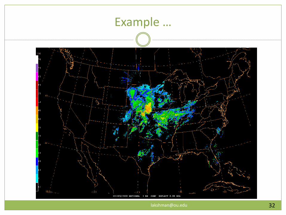
Extrapolating images
31
Extrapolation of radar echoes
Intuitive approach: “put” Take current echoes
Move them forward in time (advect) by their motion field
“put” is subject to holes in the created images “get” results in the wrong motion field being used
Simple “put” followed by “get” Move echoes forward, fill in gaps via interpolation
Results in ghost echoes
Smarter approach: Advect the motion field, interpolating within gaps
Now, do “get” using advected motion field

2-hour forecasts 33
Radar observations
advection
HRRR


Morphing (0-4 hour) 35

Data Mining Storm Attributes
36
Introduction
Storm Identification
Storm Association
Extracting Storm characteristics
Estimating Motion
Nowcasting
Backmatter
segmotion is a general-purpose algorithm
Segmentation + Motion Estimation Segmentation --> identifying parts (“segments”) of an image Here, the parts to be identified are storm cells
segmotion consists of image processing steps for: Identifying cells Estimating motion Associating cells across time Extracting cell properties Advecting grids based on motion field
segmotion is part of WDSS-II Can be downloaded from http://www.wdssii.org/ Can be applied to any uniform spatial grid
Has been applied to radar, satellite, model grids, 2D/3D lightning Some applications interested only in advection; others only on attribute extraction
37

Try things out …
38
Download WDSS-II from http://www.wdssii.org/ Follow “Quick Start” to learn how to run algorithms
Download radar data from NCDC Convert to netcdf using ldm2netcdf
Use –c option to create composite
Run w2segmotioncg on ReflectivityComposite
Experiment with various options as described on the following slides
Try applying QC/smoothing to data first
w2qcnn or w2qcnndp
w2smooth (or –k option to w2segmotioncg)
WDSS-II w2segmotionll References
39
Algorithm for identifying and tracking cells from spatial grids Identify cells using vector quantization and watershed transform [2] Estimate motion using cross-correlation and interpolation [1] Track cells: longevity, size-based search radius and cost function [4] Extract attributes: geometric, spatial and temporal [3]
How to evaluate algorithm: Evaluate cell tracks using mismatches, jumps & duration [4] Evaluate motion field using advected products [1]
1) V. Lakshmanan, R. Rabin, and V. DeBrunner, ``Multiscale storm identification and forecast,'' J. Atm.
Res., vol. 67, pp. 367-380, July 2003. 2) V. Lakshmanan, K. Hondl, and R. Rabin, ``An efficient, general-purpose technique for identifying
storm cells in geospatial images,'' J. Ocean. Atmos. Tech., vol. 26, no. 3, pp. 523-37, 2009. 3) V. Lakshmanan and T. Smith, ``Data mining storm attributes from spatial grids,'' J. Ocea. and Atmos.
Tech., vol. 26, no. 11, pp. 2353-2365, 2009 4) V. Lakshmanan and T. Smith, ``An objective method of evaluating and devising storm tracking
algorithms,'' Wea. and Forecasting, vol. 25, no. 2, pp. 721-729, 2010.

WDSS-II Programs
40
w2segmotionll Multiscale cell identification and tracking: this is the program that much of this talk refers to.
w2advectorll Uses the motion estimates produced by w2segmotionll (or any other motion estimate, such as that from a model) to project a spatial field forward
w2scoreforecast The program used to evaluate a motion field. This is how the MAE and CSI charts were created
w2scoretrack The program used to evaluate a cell track. This is how the mismatch, jump and duration bar plots were created.
w2morphtrack Combines HRRR forecasts with advection to provide skillful nowcasts over longer time periods