nowpdf writer, job 49

Copyright

by

Akinleye Olaolu Alawode

2005

Oxidative Degradation of Piperazine in the

Absorption of Carbon Dioxide

by

Akinleye Olaolu Alawode, B.S.

Thesis

Presented to the Faculty of the Graduate School

of The University of Texas at Austin

in Partial Fulfilment

of the Requirements

for the Degree of

Master of Science in Engineering

The University of Texas at Austin

May, 2005

Oxidative Degradation of Piperazine in the

Absorption of Carbon Dioxide

APPROVED BY

SUPERVISING COMMITTEE:

_____________________________ (SUPERVISOR) GARY ROCHELLE

_____________________________ BRUCE ELDRIDGE

Dedication

To Jesus Christ my Lord and Savior

v

Acknowledgments

To God Almighty for giving me this opportunity, and for being with me

since the beginning of my program all the way to the end.

I would like to thank Dr. Gary Rochelle whose support and contributions to this

work are immeasurable and without whom I would not even be here in the first

place. He gave me the much needed encouragement at times when I hit road

blocks in my research, finding a way to make me push forward and overcome the

problems.

I am also grateful for the financial support from the Separations Research

Program and the Texas Advanced Technology Program. I thank Dr. Mullins who

gave me a chance to prove myself and provided me with the much needed

guidance throughout the course of my stay in Austin. Thanks for being a friend.

I would also like to acknowledge my family for supporting me when I

came over to the United States. Finally, to the most important person in my life,

my wife who believed in me and was my major source of motivation throughout

this program. Thanks for being there with me every step of the way. I love you

very much.

May 2005

Austin, Texas

vi

Oxidative Degradation of Piperazine in the Absorption of

Carbon Dioxide

by

Akinleye Olaolu Alawode, M.S.E.

The University of Texas at Austin, 2005

SUPERVISOR: Gary T. Rochelle

Oxidative degradation of piperazine was quantified by using Gas and Ion

Chromatography. The GC analysis involved the direct analysis of the piperazine

using calibration standards, while the IC analysis was based on quantifying

acetate, a degradation product which is an indication of piperazine loss. This

study used an agitated reactor maintained at 55oC, with conditions similar to those

in absorber/stripper configurations for CO2 removal from flue gas.

The problems encountered with the apparatus by the previous

investigator were eliminated and the effect of varying some process parameters

such as catalyst concentration, duration and agitation on degradation was studied.

The rate of acetate production ranged from 0.08 to 0.4mM/hr while actual

piperazine loss ranged from 1mM/hr to 5mM/hr. The degradation rate was found

to be dependent on agitation rate and catalyst concentration.

vii

Table of Contents

CHAPTER 1 Introduction…………….………………………………………….1

1.1. Background……………………………………………………………….1

1.2. Importance of degradation…………………………………………………5

CHAPTER 2 Analytical Methods…….…………………………………………11

2.1. Gas Chromatography……………………………………………………...11

2.1.1. GC Method Development…………………………………………… 13

2.2. Ion Chromatography…………..……..…………..………………………17

2.2.1. IC Method Development.....…………………………………………..18

2.3. Nuclear Magnetic Resonance…………………………………………… 22

2.3.1. The NMR Method……...………………….…………………………..23

CHAPTER 3 Oxidative Degradation…….………….…………………………..26

3.1. Experimental Apparatus…………………………………………………..26

3.2. Experimental Procedure…………………………………………………..30

CHAPTER 4 Results…………………….……………………………..………..33

4.1. Summary of Experimental Results……….…..………………..………….33

CHAPTER 5 Conclusions and Recommendations…………..………………….40

5.1. Results………………………….……………………………..…………..40

5.2. Apparatus and Sample Analysis…………………………………………. 42

viii

APPENDIX A Raw Results………………………………................................44

APPENDIX B Procedure for Using the GC........................................................46

APPENDIX C Ion Chromatograms.....................................................................65

C.1. Analytical Information.............................................................................65

C.2. Sample Preparation...................................................................................65

C.3. Procedure for IC.......................................................................................66

APPENDIX D NMR Peaks and Positions...........................................................73

References.............................................................................................................79

Vita........................................................................................................................82

ix

List of Tables

Table 4.1. Summary of Experimental Results.………………………………..…35

Table A.1. Peak Areas from GC……………..…………………………………..44

Table A.2. Concentration of PZ after Calibration.………………...……………. 45

Table A.3. Concentration Values from IC…...……………………………..……45

Table D.5. Position for Peaks in NMR Spectra…...…………………..…………73

x

List of Figures

Figure 1.1. Schematics of a Typical Acid Gas Removal Process………………...4

Figure 2.1. A Typical Calibration Curve Showing Linear Response of the GC..13

Figure 2.2. Chromatogram Showing Piperazine and Ethanol...............................16

Figure 2.3. Sample Chromatogram of Formate....................................................20

Figure 2.4. Sample Chromatogram of Acetate.....................................................21

Figure 2.5. Sample Chromatogram of Glycolate..................................................21

Figure 2.6. Calibration Curve of Ion Chromatograph............................................22

Figure 2.7. NMR Spectrum Showing Piperazine, Formate and Acetate..............25

Figure 3.1a. Experimental Set-up.........................................................................28

Figure 3.1b. Reactor Cover (Top View)...............................................................29

Figure 4.1. Chromatogram for Experiment 1-4-2005...........................................37

Figure 4.2. Chromatogram for 1-2-2005...............................................................37

Figure 4.3. Chromatogram for 12-20-2004...........................................................38

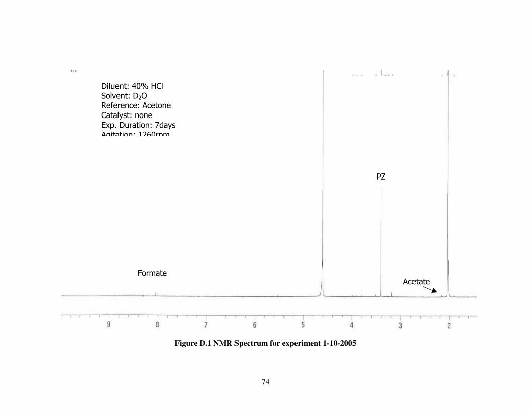
Figure 4.4. Chromatogram for 1-10-2005.............................................................38

Figure 4.5. Chromatogram for 12-22-2004...........................................................39

Figure B.1. Chromatogram for 6-13-2004, Initial................................................50

Figure B.2. Chromatogram for 6-13-2004, Final..................................................51



xi





Figure B.9. Chromatogram for Calibration Sample1............................................58

Figure B.10. Chromatogram for Calibration Sample 2.........................................59



Figure B.13. Calibration Curve for 6-21-2004.....................................................62



Figure C.1. Calibration Curve for 1-10-2005.......................................................68

Figure C.2. Calibration Curve for 12-20-2004.....................................................69

Figure C.3. Calibration Curve for 1-2-2005.........................................................70

Figure C.4. Calibration Curve for 1-4-2005.........................................................71

Figure C.5. Calibration Curve for 12-22-2004.....................................................72

Figure D.1. NMR Spectrum for experiment 1-10-2005......................................74

Figure D.2. NMR Spectrum for experiment 12-20-2004....................................75

Figure D.3. NMR Spectrum for experiment 1-4-2005........................................76

Figure D.4. NMR Spectrum for experiment 12-22-2004.....................................77

Figure D.5. NMR Spectrum for experiment 1-2-2005.........................................78

1

CHAPTER 1

Introduction

Greenhouse gas emissions have become important with a growing

awareness of their impact on global climate change. In the United States alone,

approximately fifteen thousand pounds of carbon equivalent greenhouse gases are

emitted per person every year, eighty-two percent of which come from coal-fired

power plants and automobiles. This is why significant research effort has been

channeled towards technology for CO2 capture and sequestration. This research is

focused on investigating the oxidative degradation of a potential replacement

solvent.

1.1. Background

Many processes have been developed for acid gas removal. The

Absorption/stripping with amine solutions has extensive industrial applications

(Figure 1.1). In this configuration, flue gas enters the absorber from the bottom

while the amine solution flows down from the top. The amine contacts the gas

2

counter currently with the CO2 transferring into the solution. After the loaded

solution leaves the bottom of the absorber, it is heated in the heat exchanger and

fed into the top of the stripper where it contacts steam produced in the reboiler at

reduced pressure and high temperature. The energy supplied by the steam

reverses the reaction of the gas with the amine, increasing the partial pressure of

the gas and thereby stripping it from the solution. The lean solution is sent to the

heat exchanger where the temperature is reduced before it is returned to the

absorber. The flue gas can contain as much as 12 mole percent CO2 and 5 mole

percent O2. The absorber usually operates at 40-60oC and 1 atm while the stripper

is usually at 100-120oC and 1 to 2 atm.

One of the most common solvents used in this process is 15-30 wt-%

monoethanolamine (MEA) solution, which has been considered the state-of-the-

art solvent in spite of its shortcomings. This is probably because of the difficulty

in finding a solvent that combines cheapness of raw materials with high rate and

capacity for CO2 absorption, as is the case with MEA. As the issue of greenhouse

gases became more important, there has been the pressure to find more efficient

and economical ways of removing greenhouse gases. Thus, the main focus of

recent research has been finding other solvents that are as good as, or even better

than MEA, without sharing its disadvantages.

One of the major problems of MEA is its high heat of CO2 absorption;

18.9 kcal/gmol at 25oC and 23.6 kcal/gmol at 120oC (Austgen, 1989). This makes

3

the absorption process with MEA highly energy-intensive, driving up cost. MEA

has a very high degradation rate and this also drives up the cost for raw materials

because of the need for frequent replacement and disposal of the spent solvent.

Finally, MEA has the highest corrosion rate of carbon steel when compared to all

the other known amines and this has a direct effect on the equipment.

One of the solvents that is currently being tested as a possible replacement

for MEA is potassium carbonate promoted with piperazine (Cullinane, 2005). On

its own, potassium carbonate does not have the rate and capacity for CO2 that

MEA has, but this is greatly improved by the addition of piperazine (PZ),

Cullinane (2002). In choosing piperazine as a promoter, it was also important to

ensure that it would not drive up the heat of absorption of the mixture as most

amines do. Apart from having rates and capacity comparable to or even better

than that of MEA at certain concentrations, the heat of absorption for the

potassium carbonate solvent is 6.3 kcal/gmol at 25oC and 3.0 kcal/gmol at 120oC.

Piperazine is a secondary amine and because it is key to the properties of

potassium, its kinetics and chemistry, of which little is currently known, has to be

fully understood.

PZ is five times more expensive than MEA. Therefore it must have a

lower rate of degradation than MEA if it is to be economically viable.. It is also

important to have an understanding of the degradation by-products and their

impact on the internals of the absorber-stripper system in terms of corrosion as

4

well as for reasons of disposal. In conclusion, if PZ-promoted potassium

carbonate is to be economically viable industrially, the degradation process must

be studied. Therefore this research is focused on understanding and quantifying

the oxidative degradation of piperazine in aqueous potassium carbonate.

UntreatedGas Stream

TreatedGas Stream

RichSolvent

LeanSolvent Heat Source

Captured GasCO2, H2S, H2O

UntreatedGas Stream

TreatedGas Stream

RichSolvent

LeanSolvent Heat Source

Captured GasCO2, H2S, H2O

Figure 1.1 CO2 Capture by Aqueous Absorption/Stripping

1 – 2 atm 120oC

1 atm 55oC

5

1.2. Importance of Degradation

A major factor in determining the economic viability of a solvent is the

rate at which it degrades. Thus, apart from having absorption rates and capacity

comparable to that of MEA, a solvent either has to be cheaper or have a lower rate

of degradation before it can be considered as a possible replacement. Degradation

is an irreversible process and the spent solvent must be replaced. Moreover, the

waste must also be disposed of and the toxicity of the waste products is

determined mainly by the kind of degradation products that are in it. Degradation

products can also be responsible for a high degree of corrosion that occurs in the

process equipment. Degradation products expected from MEA include ammonia,

formate, acetate, formaldehyde, methyl amine and other carboxylic acids.

According to data from IEA, the cost of CO2 capture is about $35/metric ton.

MEA make-up comes to about $4.86/metric ton of CO2 (Kerr-McGee, 1992). This

shows that although degradation is not critical, it is still an important factor to

consider, contributing to about 5% of the total cost of CO2 capture. This is lower

than would be the case for a more expensive solvent because at $0.67/lb, MEA is

one of the cheapest solvents in use today.

There are two types of degradation associated with the use of amines in

stripper/absorber configurations for CO2 capture – oxidative degradation and

carbamate polymerization. Oxidative degradation requires dissolved oxygen or

metals that can be reduced. Due to the high concentration of oxygen, oxidative

6

degradation is probably limited to the absorber. Carbamate polymerization

involves amine carbamates bonding with the amino groups of free amines/amine

compounds. This requires high temperatures and CO2-loaded alkanolamines and

is most likely to occur in the stripper. Piperazine is not an alkanolamine and

should not be subject to carbamate polymerization. Therefore oxidative

degradation will be most important for the piperazine-potassium carbonate..

The chemistry of the degradation process is very complex, as is evident in

the complexity of the absorption reactions.

RNH

R'C

O

O

+R

NH2+

R'+

RN

R'C

O

O-

(1)2

The absorption of CO2 is believed to take place in two steps: the formation of a

net-neutral charged intermediate (a zwitterion) and the extraction of a proton to

yield a protonated amine and a carbamate (Equations 2 & 3).

7

C

O

O

+R

NHR'

RNH+

R'C

O-

O(2)

RNH+

R'C

O-

O+

RNH

R'

RNH2

+R'

+R

NR'

CO-

O(3)

Over the years different researchers for degradation have proposed many

mechanisms. Hull (1969) proposed a mechanism for tertiary amines from

experimental work with oxidants such as chlorine dioxide and hexacyanoferrate.

The free radical extracts an electron from the unprotonated nitrogen in the amine

and a proton leaves the adjacent carbon to form an imine radical. The reaction

can then have two different pathways. In the first half, the imine can hydrolyze to

form an aldehyde or ketone and an amine. In the second half, the imine that has

lost a constituent can be hydrolyzed to form either an aldehyde and a further

fragmented amine or organic acids and more fragmented amines. In the case of

piperazine, this mechanism would form ethylenediamine monoacetaldehyde in the

pathway that uses two oxidizers atoms and ammonia or an amine that has an

acetaldehyde group in the pathway that only needs one oxidizer. The aldehyde

8

constituents can be readily oxidized to their carboxylate counterparts (Denisov,

1977; Sajus and Seree De Roch, 1980).

In industrial applications, there is an abundance of metals in solution.

Amines are known to be highly corrosive and thus there is a supply of iron from

the process equipment. Metals such as vanadium and copper are also added to

amine solutions to act as corrosion inhibitors (Pearce et al, 1984, Faucher, 1989,

Wolcott et al, 1986). It has been shown that these metals may also help to

catalyze the degradation reaction by the pathway of free radicals (Ferris et al,

1968). Lee and Rochelle (1998) suggested that the ferrous ion reacts with

peroxides in solution, producing free radicals that can initiate oxidation:

Fe+2 + ROOH→ Fe+3 + RO• + OH-•

Fe+3 + ROOH→ Fe+2 + ROO• + H+

The ferrous ion can be regenerated by reacting with peroxide, making more free

radicals available in solution and conserving the iron that can then react with

dissolved oxygen to create ferric ion, hydrogen peroxide and hydroxyl and peroxy

radicals.

Fe+2 +O2 → Fe+3 + O2-•

Fe+2 + O2-• → Fe+3 + H2O2

9

Fe+2 + H2O2→ Fe+3 + OH-+ OH•

Fe+2 + OH• → Fe+3 + OH-

These compounds can react with the amines themselves through autoxidation. In

autoxidation, the oxygen, usually as peroxide, reacts with carbon adjacent to the

nitrogen, with either the extraction of a hydrogen, or the loss of a proton. The

radical carbon reacts with oxygen to produce more radicals and degradation

products. It is expected that this reaction mechanism will be important in the

study of degradation in piperazine.

Most of the work that has been done in the field of degradation has

involved the more popular amines like Monoethanolamine, Diethanolamine

(DEA), Diglycolamine (DGA) and Methyldiethanolamine (MDEA). Organic

acids like formic, acetic and glycolic acid have been discovered as the

degradation products of such amines. Rooney (1998) showed some of the

degradation products of MEA to be formate, acetate and glycolate, and also went

on to show that larger amine compounds such as DEA and MDEA and other

secondary and tertiary amines have similar degradation products. The rates of

oxidation for amines have been from 0.2mM/hr for MDEA to 7mM/hr for MEA

and 10mM/hr for DEA (Kindrick, 1950).

Chi (2000) and Goff (2003) have both confirmed that metal ions,

especially iron and copper, catalyze the degradation of MEA based on rate of

ammonia evolution. Chi and Rochelle established the fact that only ferrous iron

10

catalyzes ammonia production in unloaded MEA and that the rates of degradation

were two times faster in the loaded solutions in comparison to unloaded solutions.

Goff also found out that the degradation rate is a strong function of mass transfer

based on experiments conducted with 15 wt-% magnesium sulfate.

In the analysis of amines and their degradation products, different

analytical tools have been employed. Rooney (1998) used ion chromatography to

analyze for formate, acetate and glycolate. Dawodu and Meisen (1996) used gas

chromatography to analyze degradation products of MDEA and blends of MDEA,

DEA and MEA. Strazisar (2002) used gas chromatography with detection

methods such as MS and FTIR.

For this study, attempts were made to investigate the degradation of PZ by

quantifying and identifying possible degradation products in a laboratory

environment. This also involved studying the effect of corrosion inhibitors and

iron on the rate of degradation. A 2m PZ and 4m potassium bicarbonate solution

was used in the experiments. The apparatus and conditions were chosen to

simulate the conditions in an absorber. Reactor temperature was kept constant at

55oC and pure oxygen with 2% CO2 flows into the reactor to cause degradation of

the solution. Gas Chromatography, Ion Chromatography and Nuclear Magnetic

Resonance Spectroscopy (NMR) were used to measure degradation of PZ and

identify and quantify possible degradation products.

11

CHAPTER 2

Analytical Methods

2.1 Gas Chromatography (GC)

The Gas Chromatograph is a versatile analytical tool that is well suited to

the analysis of piperazine. Due to the low level of degradation expected in the

piperazine, there is a need for accuracy and reproducibility. The fact that the

solutions to be analyzed contain a high concentration of potassium salt also

impacts heavily on the method and the tool. The GC has a higher tolerance for

the potassium bicarbonate than other methods for analyzing amines while

maintaining a fairly high degree of sensitivity.

In GC, an important requirement is that the components be stable, have

different molecular weights and/or boiling points. The closer the components are

in terms of molecular weight, the more difficult the separation will be. The

components also have to be able to interact with the column material (the

stationary phase) and the mobile phase (the carrier gas), leading to differing

12

distribution of the sample components between the two phases. The choice of

carrier gas depends solely on the type of detector being used, the most important

characteristic being that it must be inert.

The components travel through the columns at rates determined by their

affinity for the solid packing of the column. The GC separates components on the

basis of boiling point, polarity or molecular weight. The boiling point is the

method of choice here because a temperature program can be incorporated into

the method development, thereby improving the separation efficiency. The

components are measured by a detector, which converts the quantity into

proportional peak areas. There are several kinds of detectors some of which are

the Flame Ionization Detector (FID), Thermal Conductivity Detector (TCD) and

Electron Capture Detector. The FID is preferred in this case because it is

particularly suited to analysis of organic compounds, has a high degree of

sensitivity and a wide linear response range (Fig. 2.1). It is also robust and very

easy to use.

In the FID, the effluent from the column is mixed with hydrogen and air

and ignited, producing ions and electrons, which conduct electricity through the

flame. A large electric potential is applied at the burner tip and a collector

electrode is located immediately above the flame. The resulting current is then

measured and converted into peak areas by the associated software. Column

13

length, gas flow rates and temperature all play a vital role in ensuring a good

separation.

Figure 2.1 A typical calibration curve showing linear response of the GC

2.1.1. GC Method Development

The GC used for this study was an HP 5890 with an HP 7673 autosampler.

The method was built round the more sensitive Flame Ionization Detector (FID),

with a 30m HP-5 capillary column and a stationary/adsorbent part made of

polyoxysiloxane. Due to the high concentration of potassium salts, samples were

diluted a factor of 100 with 1-wt% ethanol, which also served as the internal

Calibration: 1 – 2.2m PZ Injector: 200oC Detector: 200oC Oven: 80 – 200oC

14

standard and helped in normalizing the injections. The GC operated with a split

ratio of 20:1 to further reduce the load on the column, injector and detector.

Injection volume of 1µL was made fairly reproducible by using the autosampler.

Helium (99.999% purity) at a flow rate of 10mL/min was the carrier gas and

transports the volatilized components through the column. Air (350mL/min) and

hydrogen (45mL/min) were used in lighting the FID. All the gases were supplied

by Matheson Trigas. The ratio of gas flows is important because excess helium or

compressed air extinguishes the flame and makes detection impossible. All flow

rates were controlled by the mass flow controller on the GC and were measured

using a bubble flow meter.

The injector and detector temperatures were both at 200oC. The

temperature of the injector was chosen to be at least 50oC more than the boiling

point of the least volatile component expected in the matrix in order to ensure

complete volatilization of the sample. The oven operated on a temperature

program in order to improve the separation efficiency. The temperature started at

80oC and was held for 2 minutes. It is then raised to 120oC at 10oC/min, held for

another 3 minutes and finally raised to 200oC at a ramp rate of 50oC/min. The

middle ramp did an excellent job of eliminating the extreme tailing associated

with the piperazine and the final ramp prepared the column for the subsequent

injections by baking out the column. To improve the sensitivity of the analysis,

certain maintenance procedures were necessary due to the high concentration of

15

salts. After every 50 injections the septum was changed, the column was

trimmed, the injector liner and FID removed and cleaned. The GC was calibrated

using piperazine/potassium solution in water. The ratio of PZ:K+ was 1:2 and

the PZ concentrations ranged from 1.4m to 2.2m while the potassium

concentration was from 2.8m to 4.4m. This was consistent with the concentration

ratio used in all the experiments.

16

Figure 2.2 Chromatogram showing piperazine and ethanol

��

��

��

17

2.2 Ion Chromatography

With the dilution of the samples and the high split ratio it is almost

impossible to use the Gas Chromatograph in identifying degradation products,

which play an important part in quantifying piperazine losses. The IC is able to

detect concentrations as low as parts per billion. The major advantage of this is

that the samples can be diluted as much as a thousand without the system losing

its sensitivity for the degradation products.

In principle the Ion Chromatograph has some similarities to the Gas

Chromatograph although there are marked differences. For the GC, the analyte is

transported by a carrier gas and separation is by difference in boiling point or

molecular weight. In the IC, the analyte is transported by an eluent and gets

attached to the stationary fixed material of the walls (the adsorbent) of the

column. The success of the separation is based on the principle that different ions

will adhere more strongly to the column than others and hence the least strongly

attached ions elute first, followed by the next less strongly attached and so on.

For anion chromatography, the eluent is usually Na2CO3/NaHCO3 solution or

NaOH/KOH solution over a range of concentrations, depending on the particular

separation stage. The Ion Exchange Column is packed with positively charged

adsorbent material and these sites act to attract the anions from both the analyte

and the eluent. Depending on the size of the ion and the charge, some anions get

18

more tightly bound than others in solution, hence they elute much later and the

separation is effected on this basis.

The solution coming out of the column passes through a suppressor

column, which contains acidic protons to get rid of the carbonate, bicarbonate or

hydroxide ions of the eluent, making it possible for the detector to measure the

low concentrations of the anions of interest. The detector measures the electrical

conductance of the solution and this is compared to a baseline of pure distilled

deionized water. The conductance is proportional to the concentration of the ions

dissolved in the solution and the results are presented in terms of peak areas.

2.2.1. IC Method Development

The Ion Chromatograph is a Dionex DX 600 with an AS 11-HC anion

column, AG 11-HC guard column and an ULTRA II suppressor. The eluent is a

relatively high concentration of potassium hydroxide that is a strong electrolyte.

The actual concentration of the analyte anions of interest are present in the parts

per million level or less and would not be noticeable if the eluent were allowed to

pass through the column directly. This means it would be difficult if not

impossible to measure the difference in the conductivity of the pure eluent itself

and that of the anions of interest.

19

The eluent thus has to pass through the suppressor column before entering

the conductivity detector to remove the hydroxide ions from the solution. This is

what makes it possible to detect parts per billion concentrations of analytes in

samples. The suppressor column is essentially an ion exchange column that is

impregnated with acidic protons. As the eluent flows into the column, the

hydroxide ions react with the acidic protons and are removed from the solution.

The potassium ions that are left then get to fill up the vacant positions left in the

column by the acidic protons. This way, the tiny anions are able to pass through

to the conductivity detector and can then be measured.

6M Sulfuric acid was used in regenerating the suppressor. The IC uses an

AS 40 automated sampler that holds 11 cassettes of six 5mL vials. Each sample

is filtered through a 20-µm filter in the vial cap, eliminating the pre-filtering step.

In order to have an idea of the elution times of the target compounds, the IC was

first calibrated with different concentrations of the ions that had the probability of

being present in the experimental samples. 0.5 to 5 ppm solutions of formate,

acetate and glycolate were prepared and loaded into the auto sampler. The elution

times for each of the ions were noted and used as a basis for comparison when the

actual samples were analyzed. Before going into the IC, the samples were diluted

a factor of 1000 to avoid overloading the column and still be within the detection

limit of the instrument.

20

All sample and eluent preparation was carried out using distilled de-

ionized water to avoid contribution of ions in ordinary distilled water to the

baseline found in the solutions. The samples tested in the IC were formate,

acetate and glycolate. The chromatograms are shown in Figures 2.3 – 2.5. The

calibration plot (Figure 2.6) shows the accuracy of the IC and the linearity of the

concentration over the entire range.

Figure 2.3 Sample Chromatogram of Formate

��!��"��#��$%�� %�� &&��'�%(�)��%�� *+,��

21

Figure 2.4 Sample Chromatogram of Acetate

Figure 2.5 Sample Chromatogram of Glycolate

Eluent: KOH, 1.5ml/min Dilut ion Factor: 1000 Concentration: 10ppm Peak Area: 1.12µs*min

��!��"��#��$%�� %�� &&��'�%(�)��%��-�*+,��

22

Figure 2.6 Calibration Curve for Ion Chromatograph, acetate

2.3. Nuclear Magnetic Resonance

NMR spectroscopy is a powerful tool that is very useful in identifying

compounds and predicting /elucidating chemical structures. NMR is a

phenomenon that occurs when the nuclei of certain atoms are immersed in a

static, uniform magnetic field. A second rotating magnetic field is applied

��!��"��#��$%�� %��%�� #�.�# &&��

23

perpendicular to the static field by beaming radio waves on the nucleus. The

frequency of the radio wave is equal to the rate of rotation of the magnetic field.

The frequency of the radio waves is changed in steps and its absorption by the

nucleus is measured. When the frequency becomes equal to the rate of precession

of the nucleus, the spin of the nucleus flips over and absorbs the energy of the

radio waves. This gives the NMR spectrum when plotted.

The only drawback of the NMR technique is that this is only manifest in

nuclei that have a property called “spin” and not all nuclei possess this property.

This means the nuclei that do not have spin will not produce an NMR signal.

There are different NMR methods/experiments that can be performed in trying to

identify the structures of different compounds such as proton, carbon 13, 2-D and

3-D. Sometimes it takes a combination of different experiments before a structure

can be confidently arrived at. The proton or 1H experiment is the focus of

analysis.

2.3.1. The NMR Method

The proton experiment was designed around the principle that in an NMR

spectrum, different hydrogen atoms attached to carbon atoms behave differently.

This is determined by the environment of each proton, the kind of bonds by which

they are attached and the functional groups that are near them. This information

24

in turn affects the shape and position or chemical shift of the peaks in the spectra.

The number of resonance signals or peaks corresponds to the number of

equivalent groups of protons and the intensity of the signal corresponds to the

number of protons contributing to it.

At the beginning, undegraded samples were first analyzed to create a

baseline for comparison purposes. 1ml of the solution was acidified with 5ml

40% HCl to eliminate the carbamate peaks that might overlap the other peaks and

prevent them from showing up. The acidified solution was then diluted with

deuterium oxide in a 1:1 ratio to enhance and lock the signal. A drop of acetone

was added directly to the final solution in each NMR tube to serve as a reference.

After identifying extra peaks that showed up, different probable degradation

products were added to the samples in turn to see if any of the extra peaks would

be enhanced.

25

Figure 2.7 NMR spectrum showing Piperazine, Formate and Acetate

)��

'/�

$��%�� )��%��

26

CHAPTER 3

Oxidative Degradation 3.1. Experimental Apparatus and Procedure

Initial experiments involving the oxidative degradation of PZ were

conducted by Jones (2003), although he had some entrainment and evaporation

problems with his set-up. This affected the accuracy of his results. In his

experiments, air and CO2 flowed into the reactor at a combined flow rate of 1.5

L/min. To achieve mass transfer, the gas flow was sparged into the solution at

this high flow rate and this lead to the problems encountered with evaporation and

entrainment. The subsequent analytical methods thus had to be modified to

account for these anomalies, introducing some degree of error into it.

The modified set-up consisted of a 500 ml jacketed reactor, five inches

deep and three inches in diameter (Fig. 3.1a). Although the reactor is not

pressurized, it was sealed tightly with a rubber cork into which three holes were

27

drilled (Fig. 3.1b). The agitator shaft passes through the central hole into the

reactor. One of the holes was used for the gas inlet while the other was used to

insert the thermometer. All the openings were made tight with rubber septa.

The temperature in the reactor was kept constant at 55oC by circulating

water from a Lauda heating bath through the jacket. A 99.9 % purity pre-mix of

O2 with 2% CO2 at 100 ml/min was used in the reactor, thereby creating more

control over the gas flow. This significantly reduced the evaporation and

completely eliminated the issue of entrainment. The gas was presaturated in an

ace vacuum trap glass tube two inches in diameter and six inches tall, filled with

water and immersed in the Lauda heating bath to keep the temperature near 55oC.

Mass transfer was achieved by using a variable speed agitator with 1-inch

marine propellers. This made it easier to conduct experiments to investigate the

effect of mass transfer on oxidative degradation by approximating the mass

transfer as a function of the agitator speed. The gas flow rate was measured with

a Fischer Model 520 precision rotameter and the temperature in the reactor

monitored with a mercury thermometer.

28

Figure 3.1a Experimental Set Up

Presaturated Gas

Thermometer

Agitator

55oC

O2 / 2% CO2 100ml/min

H2O

29

Figure 3.1b Reactor Cover (Top View)

4.5”

Relief Hole

Agitator Opening

Thermometer

Gas Inlet

30

3.2. Experimental Procedure

The test solution of 2m piperazine and 4m potassium was prepared from

99% purity anhydrous piperazine pellets from Acros Chemicals and potassium

bicarbonate granules from Fisher Chemicals. A ratio of 1:2 for piperazine /

potassium solution is known to be most effective for CO2 absorption based on

work that has been done by Cullinane (2002). Keeping in mind that the solution

was being tested with the ultimate goal of being able to adapt it on an industrial

scale for absorber-stripper systems, certain experiments were designed with this

goal in mind. Amines are known to cause a lot of corrosion in absorbers and

strippers and this ensures that iron, which is an important metal in oxidative

degradation, is always readily available. Amine carbamates are notorious

complexing agents and are expected to increase the corrosion rate. To reduce the

corrosion rate, transition metals are sometimes added to solutions to act as

inhibitors. Vanadium and copper salts have often been used for this purpose.

Unfortunately, these inhibitors have also been known to act as catalysts in

oxidative degradation. In order to investigate the effect of these metals, varying

concentrations of iron and vanadium were added to the solutions for some of the

experiments.

The first in the series of experiments had 2 molal piperazine and 4 molal

potassium in the reactor with no metal added to serve as the control. The

31

subsequent experiments had the same composition of piperazine and potassium

with different combinations of iron and vanadium. The iron used was in the form

of Iron II sulfate granules, while the vanadium was a 96% purity Sodium

Metavanadate salt, both from Acros Chemicals. Most of the experiments were

conducted for 7 days. The samples were collected by inserting a needle into the

reactor through the relief hole and drawing 4ml with a syringe. The samples were

weighed and placed in glass bottles with rubber-sealed caps, which were then

placed in the refrigerator.

The next experiment involved the same ratio of piperazine to potassium,

50 ppm iron and 5000 ppm vanadium for a period of 4 weeks. The intention was

to provide a higher degree of confidence in the earlier experiments. The

combination of iron and vanadium was chosen because it appeared to have given

the highest piperazine loss in earlier experiments. Two samples were taken, one

at the beginning of the experiment and one after four weeks. Samples were

analyzed using the Gas Chromatograph and the Ion Chromatograph.

The last set of experiments was conducted to investigate the effect of

varying different parameters on the rate of degradation. Based on results obtained

by Goff with MEA, degradation in piperazine is also thought to be mass transfer

controlled. One of the experiments varied the speed of the agitator while keeping

other factors constant in order to check the effect mass transfer had on piperazine

32

degradation. Another set of experiments explored the effects of varying metal

concentrations on the rate of degradation.

For each of these solutions the water loss was carefully monitored by

weighing the solution at the beginning and end of each experiment. Samples were

taken at 24-hr intervals, the weight was recorded for each and all were added

together at the end of the experiment to get an idea of how much water was lost

over the duration of the experiment. For this set of 7-day experiments, the ion

chromatograph was the favored method of analysis. The method was designed

around identifying and quantifying degradation products, which would be

important indicators of piperazine losses. The change in method was necessary

because the gas chromatograph was not able to give a conclusive analysis of the

piperazine samples after seven days and the IC is more sensitive and able to detect

parts per billion concentrations.

33

CHAPTER 4

Results 4.1. Summary of Experimental Results

The results for all the experiments are summarized in Table 4.1. As

previously discussed, two methods were used to analyze the samples from the

experiments. A correction was made for the water lost in the first three

experiments and the 4-wk experiment. The water loss for the later set of

experiments was negligible, less than 0.8 percent. The GC focused on identifying

the direct loss of piperazine while the IC estimated the piperazine loss based on

acetate production. The NMR was not used extensively for quantifying the

degradation products due to the difficulty involved in identifying the numerous

peaks present in the spectrum.

34

The initial analysis was done using the GC. From Table 4.1, it is not

distinct which of the four solutions exhibited more degradation although the

solution with the combination of the iron and vanadium had a slightly lower

concentration of piperazine. This is probably due to the fact that the degradation

did not occur long enough for the GC to show a clear difference in concentration

and the difference was below the detection limit.

35

Table 4.1 Summary of Experimental Results

2.0m PZ,4.0 m K+,,55oC, 100 ml/min of 2 % CO2/98% O2

Start Date Agitation (rpm)

V (ppm)

Fe (ppm)

Time (hrs)

*PZ loss (mM/hr)

#Acetate (mM/hr) PZ Loss (%)

6-13-2004 1260 5000 50 168 1.3 - 14.1

6-21-2004 “ 0 “ “ 1.2 - 13

6-30-2004 “ 5000 0 “ 0.7 - 7

7-10-2004 “ “ 50 720 5 0.3 18

12-20-2004 “ “ “ 168 - 0.4 6.3

12-22-2004 “ - “ “ - 0.31 4.7

1-2-2005 630 “ “ “ - 0.13 1.35

1-4-2005 1260 500 5 “ - 0.37 5.4

1-10-2005 “ 0 0 “ - 0.08 0.94

* Analysis with GC and final concentration corrected for water loss # Analysis with Ion Chromatograph

36

As previously stated, experiment 7-10-2004 was conducted to have a

higher degree of confidence in the results for the first three experiments. After

correction for water loss, the PZ concentration was found to be 1.64 m,

corresponding to about 18% loss of the PZ. The analysis with the ion

chromatograph was able to detect 12 ppm acetate in the sample.

Finally, for the last set of experiments, there was acetate in the samples

tested after 7 days assuming that the rate of acetate production is representative of

the rate of degradation of the piperazine. This is in agreement with what had been

observed previously with the 4-week samples. The acetate concentration in the

experiment with lower agitation is only a quarter of the one with the higher

agitation rate. The solution with zero catalyst had the lowest concentration of

acetate.

The chromatograms for the results of IC analysis are shown in Figures 4.1

– 4.5

37

Figure 4.1 Chromatogram at the end of experiment 1-4-2005

Figure 4.2 Chromatogram for 1-2-2005

��!��"��#��$%�� %��&&��

��!��"��#��$%�� %��-&&��

38



��!��"��#��$%�� %��-��&&��

��!��"��#��$%�� %�� &&��

39


The 4-week sample was analyzed with NMR and acetate was also identified.

There were some other peaks showing up that may suggest more degradation products

which have not been identified and were not picked up by anion chromatography. The

presence of these other unknowns makes it difficult to use the NMR quantitatively but the

positions of all the peaks are documented in Appendix I.

��!��"��#��$%�� %��&&��

40

CHAPTER 5

Conclusions and Recommendations

5.1 Results

The rate of degradation of PZ observed here was about 1.3mm/hr, much lower than

the 5mm/hr obtained by Goff for MEA. This could probably be explained by a number

of factors. Piperazine degradation is limited by oxygen mass transfer when there is a

significant amount of catalyst in solution. In this case, there was a high concentration of

iron and vanadium in most of the experiments. Oxygen solubility in MEA is twice as

much as that for a mixture of piperazine and potassium bicarbonate. This is because the

presence of potassium and carbonate ions lowers the solubility significantly and thus

mass transfer of oxygen to the solution is limited by the physical solubility of the oxygen.

The estimate was based on solubility correlations by Tanaka (2000) and Tokunaga

(1994).

41

Based on visual observation, agitation rate in the MEA experiments was clearly

greater than that in the PZ experiments , which could also account for the lower rate of

degradation due to the limitation in mass transfer. This is supported by the PZ

experiments that showed that the degradation rate decreased significantly when the

agitation rate was reduced by a factor of two.

There was a noticeable effect of varying metal concentration on the rate of

degradation. The experiments showed a higher rate when both metals were present in

solution, although a single catalyst at reduced concentration was still enough to

contribute significantly to the rate. This would suggest that there was a minimum

catalyst concentration that would still be effective. At low metal concentrations the

kinetics become important, while at high metal concentration the degradation becomes

oxygen mass transfer controlled. The results were in agreement with previous work done

by Goff (2003) and Chi (2002).

Acetate was found to be an important product of PZ degradation, although it

accounts for only 12% of the total piperazine loss based on experiment 7-10-2004. The

ion chromatograph was not able to identify other degradation products, but the NMR

analysis showed more degradation products in the spectra, especially after the samples

were acidified. Acetate and formate were identified, but not the other peaks.

The gas chromatograph puts the piperazine loss at 18% of the original piperazine.

The 6% difference between IC and GC values is expected to be from the yet unidentified

peaks from the NMR analysis.

42

Experiments should be done to check effect of copper on the rate of degradation.

The concentration of piperazine and potassium should be changed to see how it affects

the rate. The flow rate of O2 and CO2 can also be varied to see how it affects degradation

rate.

5.2. Apparatus and Sample Analysis

The changes made to the apparatus were quite efficient in solving the initial

problems encountered with evaporation and entrainment, resulting in no loss of material

and approximately 5g loss of water in the worst case. The methods used in investigating

the effect of different variables on the rate of degradation were also more effective as a

result of this.

The GC methods were improved with a more efficient temperature program and

maintenance methods. In spite of the improved methods, the GC was still not well suited

to quantifying piperazine loss over short periods, though quite effective over long

durations. The temperature program did a good job of effecting excellent separation with

thin peaks while eliminating the tailing effect that might bring errors into the analysis. It

should however be noted that the separation is very poor when the initial temperature

goes beyond 80oC. For even greater accuracy, the dilution of the piperazine/potassium

solution can be increased. This will further reduce the salt effects and the likelihood of

overloading the column thereby improving accuracy. Also, the more dilute the solution

is, the easier it will be to identify piperazine loss between two different samples. This

43

will be particularly useful in the 7-day experiment, the downside being that it will be

impossible to identify degradation products using the gas chromatograph.

The ion chromatography method is well developed and would only need minor

fine tuning to make it perfect. It is however important to develop a method for cation

chromatography because it is suspected that some of the degradation products appearing

in the NMR might be identifiable using cation chromatography.

The NMR method has to be expanded and geared towards quantitative analysis.

C-H correlation holds a lot of advantages which could be explored and modified to

analyze the solutions being tested. Other NMR experiments such as 2D, C13 and Dept

experiments will also be of great value in identifying the degradation products. A better

reference other than acetone is also needed to ensure a more conclusive analysis.

44

Appendix A Raw Results

The peak areas for the samples in the first three experiments are shown in Table

A.1. These are based on GC analysis and they represent the raw values. The dates

represent start dates for each of the experiments. The actual concentrations obtained

from the peak areas after calibration are in Table A.2.

Table A.3 has the IC data showing the concentration of acetate in the last five

experiments involving different catalyst concentrations and agitation rates.

Table A.1 Peak Areas from GC

Peak Area (µV)

Time (hrs) PZ/K/Fe 6-21-2004

PZ/K/V 6-30-2004

PZ/K/Fe/V 6-13-2004

0 2021.3 2020.9 2001.0

24 2015.6 2018.1 1995.6

48 2016.3 2018.5 1992.5

72 1987.3 2009.6 1990.8

96 1952.6 2003.9 1943.5

120 1938.4 2000.5 1911.5

144 1932.13 1999.8 1904.6

168 1920.01 1998.79 1900.4

45

Table A.2 Concentration Values of PZ after Calibration

Time (hrs) PZ/K/Fe (m) 6-21-2004

PZ/K/V (m) 6-30-2004

PZ/K/Fe/V (m) 6-13-2004

0 2.0 2.0 2.0

24 1.998 1.999 1.994

48 1.998 1.999 1.991

72 1.968 1.990 1.991

96 1.933 1.986 1.942

120 1.919 1.986 1.910

144 1.913 1.983 1.903

168 1.901 1.979 1.899

Table A.3 Concentration Values from IC

1-10-2005

12-20-2004

1-2-2005

1-4-2005

12-22-2004

Initial 0 0 0 0 0 Acetate Conc. (ppm) Final 0.8 4.3 1.4 3.8 3.2

46

Appendix B

Procedure for using the GC

1. All the gases were opened and the gauges were checked to make sure they were at

least 500psi.

2. The analytical column was connected and tightened at both ends, at the inlet and

at the detector to prevent leaks.

3. The mass flow controller at the GC was opened to allow Helium to flow through

the column.

4. The first step involved measuring the flow rate of the Helium by inserting the

bubble flow meter into the detector opening.

5. The flow was calculated by using the graduation on the bubble flow meter and the

stop clock on the GC itself. The timer is graduated in units of min-1 and the

bubble flow meter is graduated in ml. The flow rate is calculated by measuring

the time it takes the soap bubble to travel a graduated distance of 1, 10 or 100ml

and simply multiplying with the time reading on the GC LED.

6. The gas flow was allowed to equilibrate before flow rates were measured.

7. After measuring the He, the air valve was opened on the GC to take

measurements. (the reading for the Air included that of the Helium)

8. To set the flow rate of the Hydrogen, the Air valve was closed and that of the

hydrogen was opened. The same procedure as measuring for air was then

47

repeated. (the GC calculates the split flow by itself as long as the desired split

ratio is known).

9. Finally, after measuring both gas flow rates, both gases were opened at the GC in

order to light the FID.

10. The injector and detector temperatures were both set at 200oC and the Detector B

was chosen, representing the FID.

11. Once the gas flows were verified, the lighter button was depressed at the GC. The

best way to make sure the FID was lit was to listen for a “pop” sound of the gases

igniting. A continuous popping sound meant the gas flow rates were off and

needed to be rechecked ( only the hydrogen and air). After hearing the pop sound,

a piece of glass was held over the detector opening and condensation was also a

confirmation of the lit FID.

12. The samples to be analyzed were transferred into small vials and loaded

into the auto sampler tray, starting at position #1.

13. The method set-up determine how the samples are going to run. The parameters

that were pre-programmed include:

• Oven temperature and ramp program

• Injector and Detector temperatures

• Injection volume

• Number of injections per sample

• The pre and post rinse for the injector needle

48

14. In developing the method, a generic method was first chosen from the list of

methods already residing on the GC and saved as a new method with the name

that could be easily recognized.

15. Getting a good analytical procedure then depended on making multiple runs of the

compounds of interest and watching the resulting chromatograms while changing

the injector, detector temperature and the oven temperature program until sharp,

repeatable peaks were obtained for the compounds. This was achieved by

experimenting with different temperatures and making adjustments as they were

needed.

16. In order to obtain a certain level of reproducibility, some maintenance was

necessary. After about 20 injections, due to the high concentration of salts in the

samples, the injector port liner was removed and cleaned by replacing the wool

trap in the glass inlet. The column was also removed at the injector and trimmed

every 100 injections.

17. Three injections were made per sample and the average was used as the final

value.

18. After finishing the analysis, the injector, detector an oven temperatures are all set

to off. The gas valves are closed at the GC and then at the cylinders.

The chromatograms for the initial and final run for each of the experiments are shown in

Figures 1a to 4b. The initial chromatograms show the samples taken at time zero, while

the final chromatograms show the end of the experiment.

49

The samples were labeled based on the start dates of each of the experiments.

The GC was re-calibrated each time the samples were to be analyzed for each experiment

set. The calibration curves are also shown.

50

Figure B.1 GC Chromatogram for 6-13-2004, Initial

Sample time: 0 days Injector: 200oC Detector: 200oC Oven: 80 – 200oC Catalysts: Fe, V Exp. Duration: 7days

��

��

51

Figure B.2 GC Chromatogram for 6-13-2004, Final

Sample time: 7 days Injector: 200oC Detector: 200oC Oven: 80 – 200oC Catalysts: Fe, V Exp. Duration: 7days

��

��-�

52


Sample time: 0 days Injector: 200oC Detector: 200oC Oven: 80 – 200oC Catalysts: Fe Exp. Duration: 7days

��

��

53


Sample time: 7 days Injector: 200oC Detector: 200oC Oven: 80 – 200oC Catalysts: Fe Exp. Duration: 7days

��

��

54


Sample time: 0 days Injector: 200oC Detector: 200oC Oven: 80 – 200oC Catalysts: V Exp. Duration: 7days

��

��

55


Sample time: 7 days Injector: 200oC Detector: 200oC Oven: 80 – 200oC Catalysts: V Exp. Duration: 7days

�� -�

56


Sample time: 0 days Injector: 200oC Detector: 200oC Oven: 80 – 200oC Catalysts: Fe, V Exp. Duration: 4wks

��-�

��

57


Sample time: 4wks Injector: 200oC Detector: 200oC Oven: 80 – 200oC Catalysts: Fe, V Exp. Duration: 4wks

��

��

58

Figure B.9 GC Chromatogram for Calibration Sample 1

Injector: 200oC Detector: 200oC Oven: 80 – 200oC

��

��0�

59



��

��

60



��

�� 0�

61



��#�

��

62

0

500

1000

1500

2000

2500

3000

0 0.5 1 1.5 2 2.5 3concentration (m)

pea

k ar

ea (

mv)

Figure B.13 GC Calibration Curve for 6-21-2004

'�%(�%��%�1*23�

Injector: 200oC Detector: 200oC Oven: 80 – 200oC Catalysts: Fe Exp. Duration: 7days

63

0

500

1000

1500

2000

2500

3000

0 0.5 1 1.5 2 2.5 3

Concentration (m)

Figure B.14 GC Calibration Curve for 6-13-2004

'�%(�%��%�1*23�

Injector: 200oC Detector: 200oC Oven: 80 – 200oC Catalysts: Fe, V Exp. Duration: 7days

64

0

500

1000

1500

2000

2500

3000

0 0.5 1 1.5 2 2.5 3

Concentration (m)

Figure B.15 GC Calibration curve for 6-30-2004

'�%(�%��%�1*23�

Injector: 200oC Detector: 200oC Oven: 80 – 200oC Catalysts: V Exp. Duration: 7days

65

Appendix C

Ion Chromatography

C.1 Analytical information

The AS11 column uses a dilute KOH eluent that is made by the eluent generator,

usually using a concentration gradient program that gradually increases the eluent

concentration as the run progresses from 2mM to 30mM. It also uses a AG 11 guard

column.

C.2 Sample Preparation

All samples were kept refrigerated and in the dark until they were ready to be

analyzed. The samples contained highly concentrated potassium salts and piperazine and

had to be diluted in order to avoid over-saturating the column. For each, 1microliter of

sample is diluted in 1ml of distilled, deionized water. The volumes were measured by

using a micropipette to ensure accuracy. There were no precipitates in the samples and

therefore there was no need to profiler them, filter caps on the sample vials being sufficient

traps for particles big enough to harm the column.

66

C.3 Procedure for IC

1. The Helium tank and deionized water valve are first opened.

2. The column oven and the conductivity detector switches are turned on and this

should automatically turn on the pump, eluent generator and auto sampler.

3. On the front panel of the pump, MENU, 8, 7 sequence gives the chance to monitor

the left and right “P-Point” values when the pump is running

4. At this time the computer and software program can be turned on

5. On the main menu bar of the software, the method is selected. This should get the

pump started and the left and right p values should settle down within a few

minutes. If they don’t, the pump will have to be primed to get the bubbles out of the

pump.

6. The run schedule can then be loaded (which is a list of all calibration and unknown

samples)

7. There should be three test samples which have to be run through the system prior to

running the calibration and unknown samples. These serve the purpose of flushing

out the column and establishing a steady baseline.

8. The next set should be calibration standards, which are listed as such in the

schedule under “Sample Type”. Two or more vials of distilled deionized water are

inserted after the calibration samples to make sure the standards are flushed out

before running the unknowns.

67

9. Last in line are two samples, one standard to make sure everything ran perfectly

and DDI water which should run under the method “shut down” that will turn off

the pump and other electronics at the end of the run.

10. After saving the run schedule, the samples are then loaded into the auto sampler

rack.

11. The Hold/Run button on the auto sampler is then depressed so that the green is lit

on the RUN side. This puts the auto sampler under the computer control.

12. From the menu bar of the software, the created schedule is then loaded and the run

started by pressing the START button.

13. The run sequence starts automatically and the first chromatogram is monitored to

make sure things are running as they should.

The calibration curves for all the experiments are shown in Figures 12 to 16. The

samples were labeled based on the start dates of each of the experiments. The IC was re-

calibrated each time the samples were to be analyzed for each experiment set.

68

0

2

4

6

8

10

12

0 20 40 60 80 100 120

concentration (ppm)

peak a

rea

Figure C.1 IC Calibration curve for 1-10-2005

&�%(�%��%�1*+,��3�

��!��"��#��$%�� %��%�� #�.�# &&��%�%�4+��5��)6��%�� &��

69

0

2

4

6

8

10

12

0 20 40 60 80 100 120

concentration (ppm)

Figure C.2 IC Calibration Curve for 12-20-2004

&�%(�%��%�1*+,��3�

��!��"��#��$%�� %��%�� #�.�# &&��%�%�4+��# &&��2"�# &&��$��)6��%�� &��

70

0

2

4

6

8

10

12

0 20 40 60 80 100 120

Concentration (ppm)

Figure C.3 IC Calibration curve for 1-2-2005

&�%(�%��%�1*+,��3�

��!��"��#��$%�� %��%�� #�.�# &&��%�%�4+��# &&��2"�# &&��$��)6��%�� &��

71

0

2

4

6

8

10

12

0 20 40 60 80 100 120

Concentration (ppm)


&�%(�%��%�1*+,��3�

��!��"��#��$%�� %��%�� #�.�# &&��%�%�4+��# &&��2"�#&&��$��)6��%�� &��

72

0

2

4

6

8

10

12

0 20 40 60 80 100 120

Concentration (ppm)


&�%(�%��%�1*+,��3�

��!��"��#��$%�� %��%�� #�.�# &&��%�%�4+��# &&��$��)6��%�� &��

73

Appendix D NMR Peaks and Positions

The table shows the different peaks with their positions as observed in the spectra

for the last five experiments.

Table D.5 Positions for Peaks in NMR Spectra

Position (ppm) Peak

2.1 Acetone

2.2 Acetate

3.2 Unknown

3.25 Unknown

3.3 Unknown

3.35 Unknown

3.40 Piperazine

3.65 Unknown

3.85 Unknown

3.90 Unknown

4.00 Unknown

4.10 Unknown

4.70 Water/Deuterium

8.10 Formate

74

Figure D.1 NMR Spectrum for experiment 1-10-2005

��- 7��8��9��)��%�%�4+�� :&��%��;%4+�)6��%�� &��

)��%��$��%��

'/�

75

Figure D.2 NMR Spectrum for 12-20-2004

��- 7��8��9��)��%�%�4+��# &&��2"�# &&��$�� :&��%��;%4+�)6��%�� &��

)��%��$��%��

)��

'/�

76


��- 7��8��9��)��%�%�4+��# &&��2"�#&&��$�� :&��%��;%4+�)6��%�� &��

)��%��

)��

'/�

$��%��

77


��- 7��8��9��)��%�%�4+��# &&��$�� :&��%��;%4+�)6��%�� &��

)��%��

)��

'/�

$��%��

78


��- 7��8��9��)��%�%�4+��# &&��2"�# &&��$�� :&��%��;%4+�)6��%�� &��

)��%��$��%��

'/� )��

79

References

Austgen, D.M. A Model of Vapor-Liquid Equilibria for Acid Gas-Alkanolamine-Water Systems. Ph.D. Dissertation, The University of Texas at Austin, 1989.

Bishnoi, S. and G. T. Rochelle. “Absorption of Carbon Dioxide into Aqueous Piperazine:

Reaction Kinetics, Mass Transfer and Solubility”. Chem. Eng. Sci 55(22), 5531-5543, 2000.

Goff, G. and G.T. Rochelle. “Monoethanolamine Degradation: O2 Mass Transfer

Effects under CO2 Capture Conditions”. Ind. Eng. Chem.Res. 43, 6400-6408, 2004.

Chi, Susan and G.T. Rochelle. Oxidative Degradation of Monoethanolamine. M.S.

Thesis, The University of Texas at Austin, 2001. Cullinane, J.T. Carbon Dioxide Absorption in Aqueous Mixtures of Potassium Carbonate

and Piperazine. M.S. Thesis, The University of Texas at Austin, 2002 Chakma, A.; Meisen A. Identification of Methyldiethanolamine Degradation Products by

Gas Chromatography-Mass Spectrometry. J Chromatography 457, 287-297, 1988.

Critchfield, J.E., L. Jenkins. Evidence of MDEA Degradation in Tail Gas Treating Plants,

Pet. Tech Quart., Spring 1999. Dang, H. CO2 Absorption Rate and Solubility in Monoethanolamine/Piperazine/Water.

M.S. Thesis, The University of Texas at Austin, 2001. Dawodu, O.F., A. Meisen. Degradation of Alkanolamine Blends by Carbon Dioxide. The

Canadian Journal of Chemical Engineering. 74, 960-966, 1996. Denisov, E.T., N.L. Mitskevich, V.E. Agabekov. Liquid-Phase Oxidation of Oxygen-

Containing Compounds. Consultants Bureau, New York, 1977. Ding, Y., M.L. Lee, D.J. Eatough. International Journal of Environmental Analytical

Chemistry, 69, 243-255, 1998. Ferris, J.P., R.D. Gerwe, G.R. Gapski. Detoxication Mechanisms III: The Scope and

Mechanism of the Iron-Catalyzed Dealkylation of Tertiary Amine Oxides. J. Org. Chem., 33, 3493-3498, 1968.

80

Hull, L.A., G.T. Davis, D.H. Rosenblatt. Oxidation of Amines VII. Chemical and Electrochemical Correlations, J. Phys. Chem. 73, 2142-2146, 1969.

Hull, L.A., G.T. Davis, D.H. Rosenblatt. Oxidation of Amines IX. Correlation of Rate

Constants for Reversible One-Electron Transfer in Amine Oxidation with Reactant potentials, JACS, 91, 6247-6250, 1969c.

Jones, Terraun and G.T. Rochelle. Oxidative Degradation of Piperazine. M.S. Thesis,

The University of Texas at Austin, 2003. Kaganoi, S. “Carbon Dioxide Absorption in Methyldiethanolamine with Piperazine or

Diethanolamine: Thermodynamic Modeling and Rate Measurements,” M.S. Thesis, The University of Texas at Austin, 1997

Kennard, M.L., A. Meisen. Mechanism and Kinetics of DEA Degradation. Ind. Eng.

Chem. Fund. 24, 129-140, 1985. Kim, C.J., G. Sartori. Kinetics and Mechanism of DEA Degradation in Aqueous

Solutions Containing Carbon Dioxide. Int. J. Chem. Kin. 16, 1257-1266, 1984. Kim, C.J. Degradation of Alkanolamines in Gas Treating Solutions: Kinetics of Di-2-

propanolamine Degradation in Aqueous Solutions Containing Carbon Dioxide. Ind. Eng. Chem. Res. 27, 1-3, 1988.

Kindrick, R.C., R.E. Reitweier, M.R. Arnold. “A Prolonged Oxidation Test on Amine

Solutions Resistant to Oxidation,” Girdler Report No. T2. 15-1-31, in “Report: Carbon Dioxide Absorbents”, Contract no. NObs-50023, by Girdler Corp., Gas Process Division, Louisville, Kentucky, for the Navy Department, Bureau of Ships, Washington 25, DC (Code 649P), June 1, 1950a.

Majahani V.V., and P.V. Danckwertz. “The Stripping of CO2 from Amine-Promoted

Potash Solutions at 100oC,” Chem. Eng. Sci., 47(8), 2037-2045, 1992. Mahajani, V.V. and J.B. Joshi. “Kinetics of Reactions Between Carbon Dioxide and

Alkanolamines”. Gas. Sep. and Purification, 2(2), 50-64, 1988. Lee, Y.J., and G.T. Rochelle. Oxidative Degradation of Organic Additives for Flue Gas

Desulfurization: Products, Kinetics, and Mechanisms,” Env. Sci. Tech. 21, 266-272, 1987.

Neta, P., R.E. Huie, A.B. Ross. Rate Constants for Reactions of Inorganic Radicals in

Aqueous Solution. J. Phys. Chem. Ref. Data., 17, No. 3, 1027, 1988.

81

Rochelle, G.T. S. Bishnoi, S. Chi, H. Dang, J. Santos. “Research Needs for CO2 Capture from Flue Gas by Aqueous Absorption Stripping”. Final Report, United States Department of Energy, Federal Energy Technology Center, P.O. No DE-AF26-99FT01029, 2000.

Rooney, P.C., M.S. DuPart, T.R. Bacon. “Oxygen’s Role in Alkanolamine Degradation,”

Hydrogen Processing, 77(7), 109, 1998. Rosenblatt, D.H., L.A. Hull, D.C. De Luca, G.T. Davis, H.K.R. Williams. Oxidations of

Amines II: Substituent Effects in Chlorine Dioxide Oxidations. JACS, 89, 1158-1163, 1967.

Rosenblatt, D.H., A.J. Hayes, B.L. Harrison, R.A. Streaty, K.A. Moore. (I) The Reaction

of Chlorine Dioxide with Triethylamine in Aqueous Solution. J. Org. Chem., 28, 2790-2794, 1963.

Sajus, L., I. Seree De Roch. The Liquid Phase Oxidation of Aldehydes. Comprehensive

Chemical Kinetics, 16, 89-124, Liquid-Phase Oxidation, Elsevier Scientific Publishing Co., Amsterdam, 1980.

Schmidt, C.E., R.F. Sprecher, B.D. Batts. Analytical Chemistry, 59, 2027-2033. Seo. D.J., and W.H. Hong. “Effect of Piperazine on the Kinetics of Carbon Dioxide with

Aqueous Solutions of 2-Amino-2-Methyl-1-Propanol,” Ind. Eng. Chem. Res. 39, 2062, 2000.

Strazisar, B.R., R.R. Anderson, C.M. White. Degradation Pathways for

Monoethanolamine in a CO2 Capture Facility. United States Department of Energy 2002.

Tosh, J.S., J.H. Field, H.E. Benson, W.P. Haynes. “Equilibrium Study of the System

Potassium Carbonate, Potassium Bicarbonate, Carbon Dioxide, and Water”. United States Department of the Interior, Bureau of Mines Report of Investigation 5484, 1959.

82

Vita

Akinleye Olaolu Alawode was born on 2nd March, 1976 in Ile-Ife, Nigeria to

Festus Akinyele Alawode and Olufunmilade Alawode. He graduated with a Bachelor of

Science degree from the Department of Chemical Engineering, Obafemi Awolowo

University, Ile-Ife, Nigeria in 2001. After a year of National Youth Service, he entered

the graduate school of Chemical Engineering at the University of Texas at Austin.

Permanent Address: 2065 SE 44th Avenue, Apt. C212 Hillsboro, Oregon 97123

This thesis was typed by the author.

nowpdf writer, job 49

Documents