ns-3 model library release ns-3.17 ns-3 project
TRANSCRIPT
ns-3 Model LibraryRelease ns-3.17
ns-3 project
May 14, 2013

CONTENTS
1 Organization 3
2 Animation 52.1 NetAnim . . . . . . . . . . . . . . . . . . . . . . . . . . . . . . . . . . . . . . . . . . . . . . . . . 5
3 Antenna Module 153.1 Design documentation . . . . . . . . . . . . . . . . . . . . . . . . . . . . . . . . . . . . . . . . . . 153.2 User Documentation . . . . . . . . . . . . . . . . . . . . . . . . . . . . . . . . . . . . . . . . . . . 163.3 Testing Documentation . . . . . . . . . . . . . . . . . . . . . . . . . . . . . . . . . . . . . . . . . . 17
4 Ad Hoc On-Demand Distance Vector (AODV) 194.1 Model Description . . . . . . . . . . . . . . . . . . . . . . . . . . . . . . . . . . . . . . . . . . . . 194.2 Usage . . . . . . . . . . . . . . . . . . . . . . . . . . . . . . . . . . . . . . . . . . . . . . . . . . . 214.3 Validation . . . . . . . . . . . . . . . . . . . . . . . . . . . . . . . . . . . . . . . . . . . . . . . . . 21
5 Applications 23
6 Bridge NetDevice 25
7 BRITE Integration 277.1 Model Description . . . . . . . . . . . . . . . . . . . . . . . . . . . . . . . . . . . . . . . . . . . . 277.2 Usage . . . . . . . . . . . . . . . . . . . . . . . . . . . . . . . . . . . . . . . . . . . . . . . . . . . 28
8 Buildings Module 318.1 Design documentation . . . . . . . . . . . . . . . . . . . . . . . . . . . . . . . . . . . . . . . . . . 318.2 User Documentation . . . . . . . . . . . . . . . . . . . . . . . . . . . . . . . . . . . . . . . . . . . 368.3 Testing Documentation . . . . . . . . . . . . . . . . . . . . . . . . . . . . . . . . . . . . . . . . . . 378.4 References . . . . . . . . . . . . . . . . . . . . . . . . . . . . . . . . . . . . . . . . . . . . . . . . 40
9 Click Modular Router Integration 419.1 Model Description . . . . . . . . . . . . . . . . . . . . . . . . . . . . . . . . . . . . . . . . . . . . 419.2 Usage . . . . . . . . . . . . . . . . . . . . . . . . . . . . . . . . . . . . . . . . . . . . . . . . . . . 429.3 Validation . . . . . . . . . . . . . . . . . . . . . . . . . . . . . . . . . . . . . . . . . . . . . . . . . 44
10 CSMA NetDevice 4510.1 Overview of the CSMA model . . . . . . . . . . . . . . . . . . . . . . . . . . . . . . . . . . . . . . 4510.2 CSMA Channel Model . . . . . . . . . . . . . . . . . . . . . . . . . . . . . . . . . . . . . . . . . . 4610.3 CSMA Net Device Model . . . . . . . . . . . . . . . . . . . . . . . . . . . . . . . . . . . . . . . . 4710.4 Using the CsmaNetDevice . . . . . . . . . . . . . . . . . . . . . . . . . . . . . . . . . . . . . . . . 4810.5 CSMA Tracing . . . . . . . . . . . . . . . . . . . . . . . . . . . . . . . . . . . . . . . . . . . . . . 49
i
10.6 Summary . . . . . . . . . . . . . . . . . . . . . . . . . . . . . . . . . . . . . . . . . . . . . . . . . 50
11 DSDV Routing 5111.1 DSDV Routing Overview . . . . . . . . . . . . . . . . . . . . . . . . . . . . . . . . . . . . . . . . 5111.2 References . . . . . . . . . . . . . . . . . . . . . . . . . . . . . . . . . . . . . . . . . . . . . . . . 52
12 DSR Routing 5312.1 DSR Routing Overview . . . . . . . . . . . . . . . . . . . . . . . . . . . . . . . . . . . . . . . . . 5312.2 DSR Instructions . . . . . . . . . . . . . . . . . . . . . . . . . . . . . . . . . . . . . . . . . . . . . 5512.3 Helper . . . . . . . . . . . . . . . . . . . . . . . . . . . . . . . . . . . . . . . . . . . . . . . . . . 5512.4 Examples . . . . . . . . . . . . . . . . . . . . . . . . . . . . . . . . . . . . . . . . . . . . . . . . . 5612.5 Validation . . . . . . . . . . . . . . . . . . . . . . . . . . . . . . . . . . . . . . . . . . . . . . . . . 5612.6 References . . . . . . . . . . . . . . . . . . . . . . . . . . . . . . . . . . . . . . . . . . . . . . . . 56
13 Emulation Overview 5713.1 File Descriptor NetDevice . . . . . . . . . . . . . . . . . . . . . . . . . . . . . . . . . . . . . . . . 5913.2 Tap NetDevice . . . . . . . . . . . . . . . . . . . . . . . . . . . . . . . . . . . . . . . . . . . . . . 66
14 Energy Framework 7314.1 Model Description . . . . . . . . . . . . . . . . . . . . . . . . . . . . . . . . . . . . . . . . . . . . 7314.2 Usage . . . . . . . . . . . . . . . . . . . . . . . . . . . . . . . . . . . . . . . . . . . . . . . . . . . 74
15 Flow Monitor 77
16 Internet Models 7916.1 Internet Stack . . . . . . . . . . . . . . . . . . . . . . . . . . . . . . . . . . . . . . . . . . . . . . . 7916.2 IPv4 . . . . . . . . . . . . . . . . . . . . . . . . . . . . . . . . . . . . . . . . . . . . . . . . . . . . 8216.3 IPv6 . . . . . . . . . . . . . . . . . . . . . . . . . . . . . . . . . . . . . . . . . . . . . . . . . . . . 8216.4 Routing overview . . . . . . . . . . . . . . . . . . . . . . . . . . . . . . . . . . . . . . . . . . . . . 8416.5 TCP models in ns-3 . . . . . . . . . . . . . . . . . . . . . . . . . . . . . . . . . . . . . . . . . . . 90
17 LTE Module 9717.1 Design Documentation . . . . . . . . . . . . . . . . . . . . . . . . . . . . . . . . . . . . . . . . . . 9717.2 User Documentation . . . . . . . . . . . . . . . . . . . . . . . . . . . . . . . . . . . . . . . . . . . 16817.3 Testing Documentation . . . . . . . . . . . . . . . . . . . . . . . . . . . . . . . . . . . . . . . . . . 18917.4 Profiling Documentation . . . . . . . . . . . . . . . . . . . . . . . . . . . . . . . . . . . . . . . . . 20717.5 References . . . . . . . . . . . . . . . . . . . . . . . . . . . . . . . . . . . . . . . . . . . . . . . . 213
18 Mesh NetDevice 215
19 MPI for Distributed Simulation 21719.1 Current Implementation Details . . . . . . . . . . . . . . . . . . . . . . . . . . . . . . . . . . . . . 21719.2 Running Distributed Simulations . . . . . . . . . . . . . . . . . . . . . . . . . . . . . . . . . . . . 21819.3 Tracing During Distributed Simulations . . . . . . . . . . . . . . . . . . . . . . . . . . . . . . . . . 220
20 Mobility 22120.1 Model Description . . . . . . . . . . . . . . . . . . . . . . . . . . . . . . . . . . . . . . . . . . . . 22120.2 Usage . . . . . . . . . . . . . . . . . . . . . . . . . . . . . . . . . . . . . . . . . . . . . . . . . . . 22420.3 Validation . . . . . . . . . . . . . . . . . . . . . . . . . . . . . . . . . . . . . . . . . . . . . . . . . 227
21 Network Module 22921.1 Packets . . . . . . . . . . . . . . . . . . . . . . . . . . . . . . . . . . . . . . . . . . . . . . . . . . 22921.2 Error Model . . . . . . . . . . . . . . . . . . . . . . . . . . . . . . . . . . . . . . . . . . . . . . . 24021.3 Node and NetDevices Overview . . . . . . . . . . . . . . . . . . . . . . . . . . . . . . . . . . . . . 24221.4 Sockets APIs . . . . . . . . . . . . . . . . . . . . . . . . . . . . . . . . . . . . . . . . . . . . . . . 24421.5 Simple NetDevice . . . . . . . . . . . . . . . . . . . . . . . . . . . . . . . . . . . . . . . . . . . . 247
ii
21.6 Queues . . . . . . . . . . . . . . . . . . . . . . . . . . . . . . . . . . . . . . . . . . . . . . . . . . 247
22 Optimized Link State Routing (OLSR) 25122.1 Model Description . . . . . . . . . . . . . . . . . . . . . . . . . . . . . . . . . . . . . . . . . . . . 25122.2 Usage . . . . . . . . . . . . . . . . . . . . . . . . . . . . . . . . . . . . . . . . . . . . . . . . . . . 25222.3 Validation . . . . . . . . . . . . . . . . . . . . . . . . . . . . . . . . . . . . . . . . . . . . . . . . . 252
23 OpenFlow switch support 25323.1 Model Description . . . . . . . . . . . . . . . . . . . . . . . . . . . . . . . . . . . . . . . . . . . . 25323.2 Usage . . . . . . . . . . . . . . . . . . . . . . . . . . . . . . . . . . . . . . . . . . . . . . . . . . . 25423.3 Validation . . . . . . . . . . . . . . . . . . . . . . . . . . . . . . . . . . . . . . . . . . . . . . . . . 256
24 PointToPoint NetDevice 25724.1 Overview of the PointToPoint model . . . . . . . . . . . . . . . . . . . . . . . . . . . . . . . . . . 25724.2 Point-to-Point Channel Model . . . . . . . . . . . . . . . . . . . . . . . . . . . . . . . . . . . . . . 25824.3 Using the PointToPointNetDevice . . . . . . . . . . . . . . . . . . . . . . . . . . . . . . . . . . . . 25824.4 PointToPoint Tracing . . . . . . . . . . . . . . . . . . . . . . . . . . . . . . . . . . . . . . . . . . . 258
25 Propagation 26125.1 PropagationLossModel . . . . . . . . . . . . . . . . . . . . . . . . . . . . . . . . . . . . . . . . . . 26125.2 PropagationDelayModel . . . . . . . . . . . . . . . . . . . . . . . . . . . . . . . . . . . . . . . . . 265
26 Statistical Framework 26726.1 Goals . . . . . . . . . . . . . . . . . . . . . . . . . . . . . . . . . . . . . . . . . . . . . . . . . . . 26726.2 Overview . . . . . . . . . . . . . . . . . . . . . . . . . . . . . . . . . . . . . . . . . . . . . . . . . 26726.3 To-Do . . . . . . . . . . . . . . . . . . . . . . . . . . . . . . . . . . . . . . . . . . . . . . . . . . . 26826.4 Approach . . . . . . . . . . . . . . . . . . . . . . . . . . . . . . . . . . . . . . . . . . . . . . . . . 26826.5 Example . . . . . . . . . . . . . . . . . . . . . . . . . . . . . . . . . . . . . . . . . . . . . . . . . 269
27 Topology Input Readers 277
28 UAN Framework 27928.1 Model Description . . . . . . . . . . . . . . . . . . . . . . . . . . . . . . . . . . . . . . . . . . . . 27928.2 Usage . . . . . . . . . . . . . . . . . . . . . . . . . . . . . . . . . . . . . . . . . . . . . . . . . . . 28528.3 Validation . . . . . . . . . . . . . . . . . . . . . . . . . . . . . . . . . . . . . . . . . . . . . . . . . 288
29 Wifi 29129.1 Overview of the model . . . . . . . . . . . . . . . . . . . . . . . . . . . . . . . . . . . . . . . . . . 29129.2 Using the WifiNetDevice . . . . . . . . . . . . . . . . . . . . . . . . . . . . . . . . . . . . . . . . . 29229.3 The WifiChannel and WifiPhy models . . . . . . . . . . . . . . . . . . . . . . . . . . . . . . . . . . 29629.4 The MAC model . . . . . . . . . . . . . . . . . . . . . . . . . . . . . . . . . . . . . . . . . . . . . 29729.5 Wifi Attributes . . . . . . . . . . . . . . . . . . . . . . . . . . . . . . . . . . . . . . . . . . . . . . 29729.6 Wifi Tracing . . . . . . . . . . . . . . . . . . . . . . . . . . . . . . . . . . . . . . . . . . . . . . . 29829.7 References . . . . . . . . . . . . . . . . . . . . . . . . . . . . . . . . . . . . . . . . . . . . . . . . 298
30 Wimax NetDevice 29930.1 Scope of the model . . . . . . . . . . . . . . . . . . . . . . . . . . . . . . . . . . . . . . . . . . . . 29930.2 Using the Wimax models . . . . . . . . . . . . . . . . . . . . . . . . . . . . . . . . . . . . . . . . 30030.3 Wimax Attributes . . . . . . . . . . . . . . . . . . . . . . . . . . . . . . . . . . . . . . . . . . . . . 30130.4 Wimax Tracing . . . . . . . . . . . . . . . . . . . . . . . . . . . . . . . . . . . . . . . . . . . . . . 30230.5 Wimax MAC model . . . . . . . . . . . . . . . . . . . . . . . . . . . . . . . . . . . . . . . . . . . 30230.6 WimaxChannel and WimaxPhy models . . . . . . . . . . . . . . . . . . . . . . . . . . . . . . . . . 30630.7 Channel model . . . . . . . . . . . . . . . . . . . . . . . . . . . . . . . . . . . . . . . . . . . . . . 30630.8 Physical model . . . . . . . . . . . . . . . . . . . . . . . . . . . . . . . . . . . . . . . . . . . . . . 306
Bibliography 309
iii

iv

ns-3 Model Library, Release ns-3.17
This is the ns-3 Model Library documentation. Primary documentation for the ns-3 project is available in five forms:
• ns-3 Doxygen: Documentation of the public APIs of the simulator
• Tutorial, Manual, and Model Library (this document) for the latest release and development tree
• ns-3 wiki
This document is written in reStructuredText for Sphinx and is maintained in the doc/models directory of ns-3’ssource code.
CONTENTS 1

ns-3 Model Library, Release ns-3.17
2 CONTENTS
CHAPTER
ONE
ORGANIZATION
This manual compiles documentation for ns-3 models and supporting software that enable users to construct networksimulations. It is important to distinguish between modules and models:
• ns-3 software is organized into separate modules that are each built as a separate software library. Individualns-3 programs can link the modules (libraries) they need to conduct their simulation.
• ns-3 models are abstract representations of real-world objects, protocols, devices, etc.
An ns-3 module may consist of more than one model (for instance, the internet module contains models for bothTCP and UDP). In general, ns-3 models do not span multiple software modules, however.
This manual provides documentation about the models of ns-3. It complements two other sources of documentationconcerning models:
• the model APIs are documented, from a programming perspective, using Doxygen. Doxygen for ns-3 models isavailable on the project web server.
• the ns-3 core is documented in the developer’s manual. ns-3 models make use of the facilities of the core, suchas attributes, default values, random numbers, test frameworks, etc. Consult the main web site to find copies ofthe manual.
Finally, additional documentation about various aspects of ns-3 may exist on the project wiki.
A sample outline of how to write model library documentation can be found in src/template/doc.
The remainder of this document is organized alphabetically by module name.
If you are new to ns-3, you might first want to read below about the network module, which contains some fundamentalmodels for the simulator. The packet model, models for different address formats, and abstract base classes for objectssuch as nodes, net devices, channels, sockets, and applications are discussed there.
3

ns-3 Model Library, Release ns-3.17
4 Chapter 1. Organization
CHAPTER
TWO
ANIMATION
Animation is an important tool for network simulation. While ns-3 does not contain a default graphical animationtool, we currently have two ways to provide animation, namely using the PyViz method or the NetAnim method. ThePyViz method is described in http://www.nsnam.org/wiki/index.php/PyViz.
We will describe the NetAnim method briefly here.
2.1 NetAnim
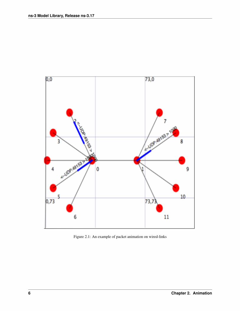
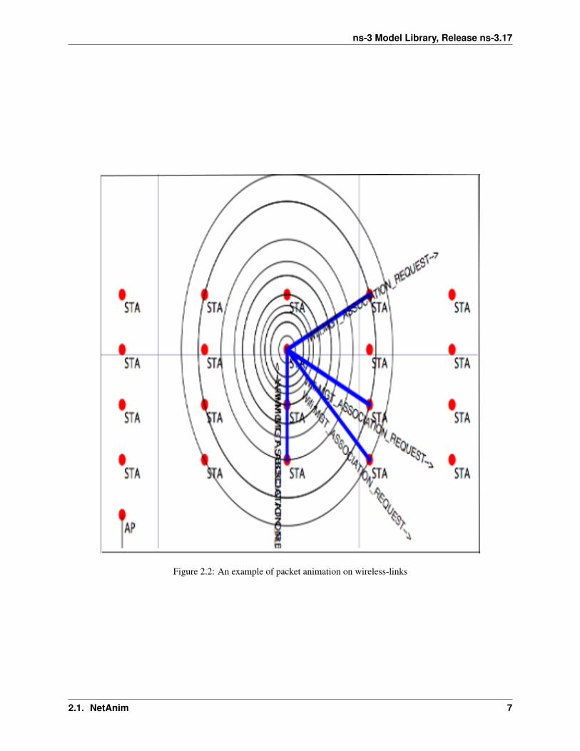
NetAnim is a standalone, Qt4-based software executable that uses a trace file generated during an ns-3 simulation todisplay the topology and animate the packet flow between nodes.
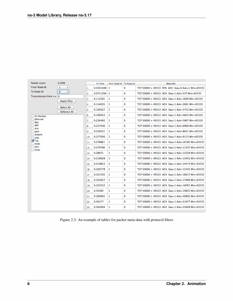
In addition, NetAnim also provides useful features such as tables to display meta-data of packets like the image below
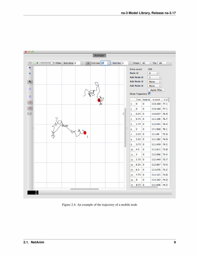
and a way to visualize the trajectory of a mobile node
2.1.1 Methodology
The class ns3::AnimationInterface is responsible for the creation the trace XML file. AnimationInterface uses thetracing infrastructure to track packet flows between nodes. AnimationInterface registers itself as a trace hook for tx andrx events before the simulation begins. When a packet is scheduled for transmission or reception, the correspondingtx and rx trace hooks in AnimationInterface are called. When the rx hooks are called, AnimationInterface will beaware of the two endpoints between which a packet has flowed, and adds this information to the trace file, in XMLformat along with the corresponding tx and rx timestamps. The XML format will be discussed in a later section. It isimportant to note that AnimationInterface records a packet only if the rx trace hooks are called. Every tx event mustbe matched by an rx event.
2.1.2 Downloading NetAnim
If NetAnim is not already available in the ns-3 package you downloaded, you can do the following:
Please ensure that you have installed mercurial. The latest version of NetAnim can be downloaded using mercurialwith the following command:
hg clone http://code.nsnam.org/netanim
5
ns-3 Model Library, Release ns-3.17
Figure 2.1: An example of packet animation on wired-links
6 Chapter 2. Animation
ns-3 Model Library, Release ns-3.17
Figure 2.2: An example of packet animation on wireless-links
2.1. NetAnim 7
ns-3 Model Library, Release ns-3.17
Figure 2.3: An example of tables for packet meta-data with protocol filters
8 Chapter 2. Animation
ns-3 Model Library, Release ns-3.17
Figure 2.4: An example of the trajectory of a mobile node
2.1. NetAnim 9
ns-3 Model Library, Release ns-3.17
2.1.3 Building NetAnim
Prerequisites
Qt4 (4.7 and over) is required to build NetAnim. This can be obtained using the following ways:
For Debian/Ubuntu Linux distributions:
apt-get install qt4-dev-tools
For Red Hat/Fedora based distribution:
yum install qt4yum install qt4-devel
For Mac/OSX:
http://qt.nokia.com/downloads/
Build steps
To build NetAnim use the following commands:
cd netanimmake cleanqmake NetAnim.pro (For MAC Users: qmake -spec macx-g++ NetAnim.pro)make
Note: qmake could be “qmake-qt4” in some systems
This should create an executable named “NetAnim” in the same directory:
john@john-VirtualBox:~/netanim$ ls -l NetAnim-rwxr-xr-x 1 john john 390395 2012-05-22 08:32 NetAnim
2.1.4 Usage
Using NetAnim is a two-step process
Step 1:Generate the animation XML trace file during simulation using “ns3::AnimationInterface” in the ns-3 codebase.
Step 2:Load the XML trace file generated in Step 1 with the offline Qt4-based animator named NetAnim.
Step 1: Generate XML animation trace file
The class “AnimationInterface” under “src/netanim” uses underlying ns-3 trace sources to construct a timestampedASCII file in XML format.
Examples are found under src/netanim/examples Example:
./waf -d debug configure --enable-examples
./waf --run "dumbbell-animation"
The above will create an XML file dumbbell-animation.xml
10 Chapter 2. Animation
ns-3 Model Library, Release ns-3.17
Mandatory
1. Ensure that your program’s wscript includes the “netanim” module. An example of such a wscript is atsrc/netanim/examples/wscript.
2. Include the header [#include “ns3/netanim-module.h”] in your test program
3. Add the statement
AnimationInterface anim ("animation.xml");where "animation.xml" is any arbitrary filename
[for versions before ns-3.13 you also have to use the line “anim.SetXMLOutput() to set the XML mode and also useanim.StartAnimation();]
Optional
The following are optional but useful steps:
1.anim.SetMobilityPollInterval (Seconds (1));
AnimationInterface records the position of all nodes every 250 ms by default. The statement above sets the periodicinterval at which AnimationInterface records the position of all nodes. If the nodes are expected to move very little, itis useful to set a high mobility poll interval to avoid large XML files.
2. anim.SetConstantPosition (Ptr< Node > n, double x, double y);
AnimationInterface requires that the position of all nodes be set. In ns-3 this is done by setting an associated Mobili-tyModel. “SetConstantPosition” is a quick way to set the x-y coordinates of a node which is stationary.
3. anim.SetStartTime (Seconds(150)); and anim.SetStopTime (Seconds(150));
AnimationInterface can generate large XML files. The above statements restricts the window between which Ani-mationInterface does tracing. Restricting the window serves to focus only on relevant portions of the simulation andcreating manageably small XML files
4. AnimationInterface anim ("animation.xml", 50000);
Using the above constructor ensures that each animation XML trace file has only 50000 packets. For example, ifAnimationInterface captures 150000 packets, using the above constructor splits the capture into 3 files
animation.xml - containing the packet range 1-50000
animation.xml-1 - containing the packet range 50001-100000
animation.xml-2 - containing the packet range 100001-150000
5. anim.EnablePacketMetadata (true);
With the above statement, AnimationInterface records the meta-data of each packet in the xml trace file. Metadatacan be used by NetAnim to provide better statistics and filter, along with providing some brief information about thepacket such as TCP sequence number or source & destination IP address during packet animation.
CAUTION: Enabling this feature will result in larger XML trace files. Please do NOT enable this feature when usingWimax links.
2.1. NetAnim 11
ns-3 Model Library, Release ns-3.17
Step 2: Loading the XML in NetAnim
1. Assuming NetAnim was built, use the command ”./NetAnim” to launch NetAnim. Please review the section“Building NetAnim” if NetAnim is not available.
2. When NetAnim is opened, click on the File open button at the top-left corner, select the XML file generatedduring Step 1.
3. Hit the green play button to begin animation.
Here is a video illustrating this http://www.youtube.com/watch?v=tz_hUuNwFDs
2.1.5 Essential settings of NetAnim
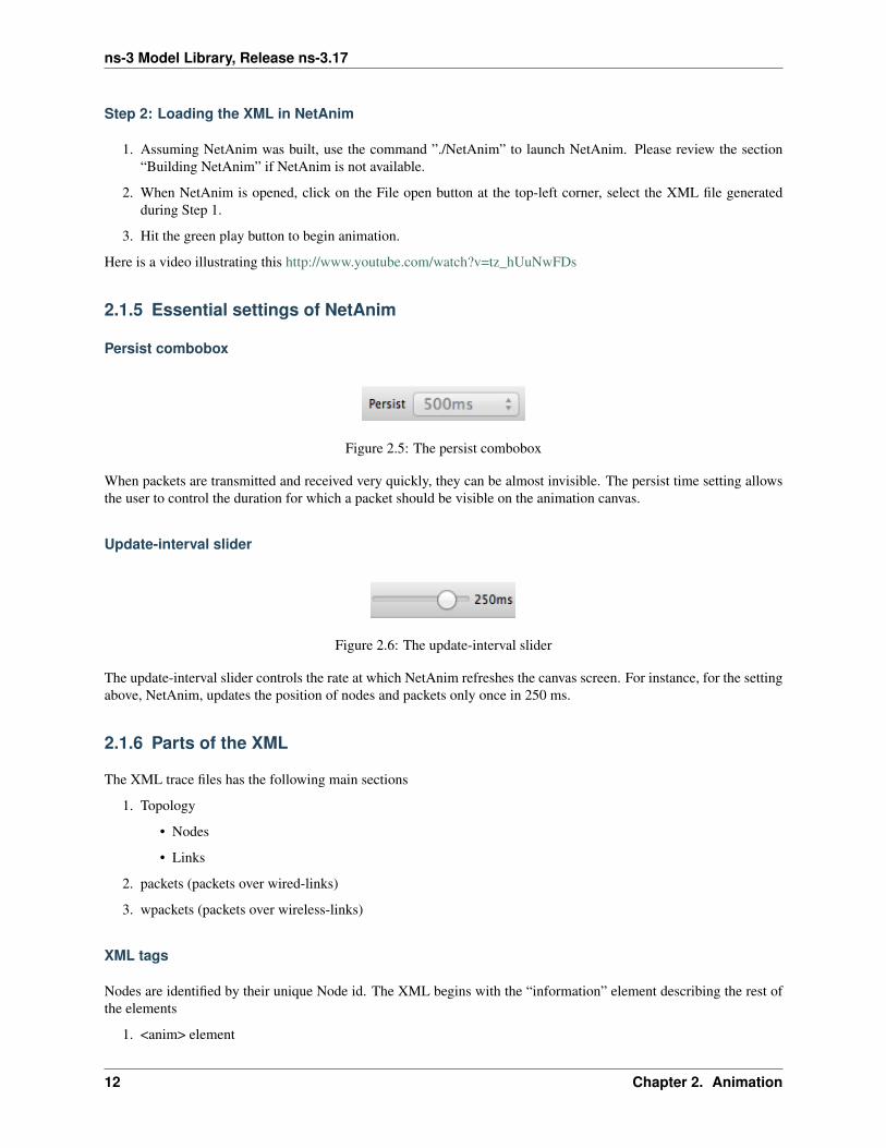
Persist combobox
Figure 2.5: The persist combobox
When packets are transmitted and received very quickly, they can be almost invisible. The persist time setting allowsthe user to control the duration for which a packet should be visible on the animation canvas.
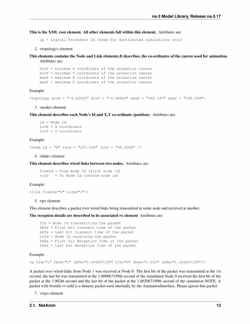
Update-interval slider
Figure 2.6: The update-interval slider
The update-interval slider controls the rate at which NetAnim refreshes the canvas screen. For instance, for the settingabove, NetAnim, updates the position of nodes and packets only once in 250 ms.
2.1.6 Parts of the XML
The XML trace files has the following main sections
1. Topology
• Nodes
• Links
2. packets (packets over wired-links)
3. wpackets (packets over wireless-links)
XML tags
Nodes are identified by their unique Node id. The XML begins with the “information” element describing the rest ofthe elements
1. <anim> element
12 Chapter 2. Animation
ns-3 Model Library, Release ns-3.17
This is the XML root element. All other elements fall within this element. Attributes are:
lp = Logical Processor Id (Used for distributed simulations only)
2. <topology> element
This elements contains the Node and Link elements.It describes, the co-ordinates of the canvas used for animation.Attributes are:
minX = minimum X coordinate of the animation canvasminY = minimum Y coordinate of the animation canvasmaxX = maximum X coordinate of the animation canvasmaxY = maximum Y coordinate of the animation canvas
Example:
<topology minX = "-6.42025" minY = "-6.48444" maxX = "186.187" maxY = "188.049">
3. <node> element
This element describes each Node’s Id and X,Y co-ordinate (position). Attributes are:
id = Node IdlocX = X coordinatelocY = Y coordinate
Example:
<node id = "8" locX = "107.599" locY = "96.9366" />
4. <link> element
This element describes wired links between two nodes. Attributes are:
fromId = From Node Id (first node id)toId = To Node Id (second node id)
Example:
<link fromId="0" toId="1"/>
5. <p> element
This element describes a packet over wired links being transmitted at some node and received at another.
The reception details are described in its associated rx element Attributes are:
fId = Node Id transmitting the packetfbTx = First bit transmit time of the packetlbTx = Last bit transmit time of the packettoId = Node Id receiving the packetfbRx = First bit Reception Time of the packetlbRx = Last bit Reception Time of the packet
Example:
<p fId="1" fbTx="1" lbTx="1.000067199" tId="0" fbRx="1.002" lbRx="1.002067199"/>
A packet over wired-links from Node 1 was received at Node 0. The first bit of the packet was transmitted at the 1stsecond, the last bit was transmitted at the 1.000067199th second of the simulation Node 0 received the first bit of thepacket at the 1.002th second and the last bit of the packet at the 1.002067199th second of the simulation NOTE: Apacket with fromId == toId is a dummy packet used internally by the AnimationInterface. Please ignore this packet
7. <wp> element
2.1. NetAnim 13
ns-3 Model Library, Release ns-3.17
This element describes a packet over wireless links being transmitted at some node and received at another.
The reception details are described in its associated rx element. Attributes are:
fromId = Node Id transmitting the packetfbTx = First bit transmit time of the packetlbTx = Last bit transmit time of the packetrange = Range of the transmission
Example:
<wp fId = "20" fbTx = "0.003" lbTx = "0.003254" range = "59.68176982" tId="32" fbRx="0.003000198" lbRx="0.003254198"/>
A packet over wireless-links from Node 20 was received at Node 32. The first bit of the packet was transmitted at the0.003th second, the last bit was transmitted at the 0.003254 second of the simulation Node 0 received the first bit ofthe packet at the 0.003000198 second and the last bit of the packet at the 0.003254198 second of the simulation
2.1.7 Wiki
For detailed instructions on installing “NetAnim”, F.A.Qs and loading the XML trace file (mentioned earlier) usingNetAnim please refer: http://www.nsnam.org/wiki/index.php/NetAnim
14 Chapter 2. Animation
CHAPTER
THREE
ANTENNA MODULE
3.1 Design documentation
3.1.1 Overview
The Antenna module provides:
1. a new base class (AntennaModel) that provides an interface for the modeling of the radiation pattern of anantenna;
2. a set of classes derived from this base class that each models the radiation pattern of different types of antennas.
3.1.2 AntennaModel
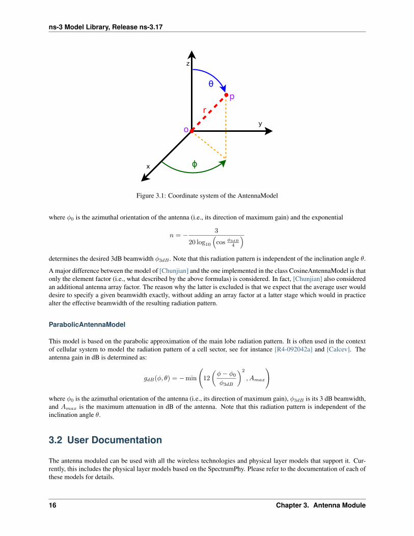
The AntennaModel uses the coordinate system adopted in [Balanis] and depicted in Figure Coordinate system of theAntennaModel. This system is obtained by traslating the cartesian coordinate system used by the ns-3 MobilityModelinto the new origin o which is the location of the antenna, and then transforming the coordinates of every genericpoint p of the space from cartesian coordinates (x, y, z) into spherical coordinates (r, θ, φ). The antenna model ne-glects the radial component r, and only considers the angle components (θ, φ). An antenna radiation pattern is thenexpressed as a mathematical function g(θ, φ) −→ R that returns the gain (in dB) for each possible direction of trans-mission/reception. All angles are expressed in radians.
3.1.3 Provided models
In this section we describe the antenna radiation pattern models that are included within the antenna module.
IsotropicAntennaModel
This antenna radiation pattern model provides a unitary gain (0 dB) for all direction.
CosineAntennaModel
This is the cosine model described in [Chunjian]: the antenna gain is determined as:
g(φ, θ) = cosn(φ− φ0
2
)
15
ns-3 Model Library, Release ns-3.17
Figure 3.1: Coordinate system of the AntennaModel
where φ0 is the azimuthal orientation of the antenna (i.e., its direction of maximum gain) and the exponential
n = − 3
20 log10
(cos φ3dB
4
)determines the desired 3dB beamwidth φ3dB . Note that this radiation pattern is independent of the inclination angle θ.
A major difference between the model of [Chunjian] and the one implemented in the class CosineAntennaModel is thatonly the element factor (i.e., what described by the above formulas) is considered. In fact, [Chunjian] also consideredan additional antenna array factor. The reason why the latter is excluded is that we expect that the average user woulddesire to specify a given beamwidth exactly, without adding an array factor at a latter stage which would in practicealter the effective beamwidth of the resulting radiation pattern.
ParabolicAntennaModel
This model is based on the parabolic approximation of the main lobe radiation pattern. It is often used in the contextof cellular system to model the radiation pattern of a cell sector, see for instance [R4-092042a] and [Calcev]. Theantenna gain in dB is determined as:
gdB(φ, θ) = −min
(12(φ− φ0
φ3dB
)2
, Amax
)
where φ0 is the azimuthal orientation of the antenna (i.e., its direction of maximum gain), φ3dB is its 3 dB beamwidth,and Amax is the maximum attenuation in dB of the antenna. Note that this radiation pattern is independent of theinclination angle θ.
3.2 User Documentation
The antenna moduled can be used with all the wireless technologies and physical layer models that support it. Cur-rently, this includes the physical layer models based on the SpectrumPhy. Please refer to the documentation of each ofthese models for details.
16 Chapter 3. Antenna Module
ns-3 Model Library, Release ns-3.17
3.3 Testing Documentation
In this section we describe the test suites included with the antenna module that verify its correct functionality.
3.3.1 Angles
The unit test suite angles verifies that the Angles class is constructed properly by correct conversion from 3Dcartesian coordinates according to the available methods (construction from a single vector and from a pair of vectors).For each method, several test cases are provided that compare the values (φ, θ) determied by the constructor to knownreference values. The test passes if for each case the values are equal to the reference up to a tolerance of 10−10 whichaccounts for numerical errors.
3.3.2 DegreesToRadians
The unit test suite degrees-radians verifies that the methods DegreesToRadians andRadiansToDegrees work properly by comparing with known reference values in a number of test cases.Each test case passes if the comparison is equal up to a tolerance of 10−10 which accounts for numerical errors.
3.3.3 IsotropicAntennaModel
The unit test suite isotropic-antenna-model checks that the IsotropicAntennaModel class works prop-erly, i.e., returns always a 0dB gain regardless of the direction.
3.3.4 CosineAntennaModel
The unit test suite cosine-antenna-model checks that the CosineAntennaModel class works properly.Several test cases are provided that check for the antenna gain value calculated at different directions and for differentvalues of the orientation, the reference gain and the beamwidth. The reference gain is calculated by hand. Each testcase passes if the reference gain in dB is equal to the value returned by CosineAntennaModel within a toleranceof 0.001, which accounts for the approximation done for the calculation of the reference values.
3.3.5 ParabolicAntennaModel
The unit test suite parabolic-antenna-model checks that the ParabolicAntennaModel class works prop-erly. Several test cases are provided that check for the antenna gain value calculated at different directions and fordifferent values of the orientation, the maximum attenuation and the beamwidth. The reference gain is calculated byhand. Each test case passes if the reference gain in dB is equal to the value returned by ParabolicAntennaModelwithin a tolerance of 0.001, which accounts for the approximation done for the calculation of the reference values.
3.3. Testing Documentation 17

ns-3 Model Library, Release ns-3.17
18 Chapter 3. Antenna Module
CHAPTER
FOUR
AD HOC ON-DEMAND DISTANCEVECTOR (AODV)
This model implements the base specification of the Ad Hoc On-Demand Distance Vector (AODV) protocol. Theimplementation is based on [rfc3561].
The model was written by Elena Buchatskaia and Pavel Boyko of ITTP RAS, and is based on the ns-2 AODV modeldeveloped by the CMU/MONARCH group and optimized and tuned by Samir Das and Mahesh Marina, University ofCincinnati, and also on the AODV-UU implementation by Erik Nordström of Uppsala University.
4.1 Model Description
The source code for the AODV model lives in the directory src/aodv.
4.1.1 Design
Class ns3::aodv::RoutingProtocol implements all functionality of service packet exchange and inheritsfrom ns3::Ipv4RoutingProtocol. The base class defines two virtual functions for packet routing and for-warding. The first one, ns3::aodv::RouteOutput, is used for locally originated packets, and the second one,ns3::aodv::RouteInput, is used for forwarding and/or delivering received packets.
Protocol operation depends on many adjustable parameters. Parameters for this functionality are attributes ofns3::aodv::RoutingProtocol. Parameter default values are drawn from the RFC and allow the en-abling/disabling protocol features, such as broadcasting HELLO messages, broadcasting data packets and so on.
AODV discovers routes on demand. Therefore, the AODV model buffers all packets whilea route request packet (RREQ) is disseminated. A packet queue is implemented in aodv-rqueue.cc. A smart pointer to the packet, ns3::Ipv4RoutingProtocol::ErrorCallback,ns3::Ipv4RoutingProtocol::UnicastForwardCallback, and the IP header are stored in thisqueue. The packet queue implements garbage collection of old packets and a queue size limit.
The routing table implementation supports garbage collection of old entries and state machine, defined in the standard.It is implemented as a STL map container. The key is a destination IP address.
Some elements of protocol operation aren’t described in the RFC. These elements generally concern cooperation ofdifferent OSI model layers. The model uses the following heuristics:
• This AODV implementation can detect the presence of unidirectional links and avoid them if necessary. If thenode the model receives an RREQ for is a neighbor, the cause may be a unidirectional link. This heuristic istaken from AODV-UU implementation and can be disabled.
19
ns-3 Model Library, Release ns-3.17
• Protocol operation strongly depends on broken link detection mechanism. The model implements two suchheuristics. First, this implementation support HELLO messages. However HELLO messages are not a goodway to perform neighbor sensing in a wireless environment (at least not over 802.11). Therefore, one may ex-perience bad performance when running over wireless. There are several reasons for this: 1) HELLO messagesare broadcasted. In 802.11, broadcasting is often done at a lower bit rate than unicasting, thus HELLO messagescan travel further than unicast data. 2) HELLO messages are small, thus less prone to bit errors than data trans-missions, and 3) Broadcast transmissions are not guaranteed to be bidirectional, unlike unicast transmissions.Second, we use layer 2 feedback when possible. Link are considered to be broken if frame transmission resultsin a transmission failure for all retries. This mechanism is meant for active links and works faster than the firstmethod.
The layer 2 feedback implementation relies on the TxErrHeader trace source, currently supported in AdhocWifiMaconly.
4.1.2 Scope and Limitations
The model is for IPv4 only. The following optional protocol optimizations are not implemented:
1. Expanding ring search.
2. Local link repair.
3. RREP, RREQ and HELLO message extensions.
These techniques require direct access to IP header, which contradicts the assertion from the AODV RFC that AODVworks over UDP. This model uses UDP for simplicity, hindering the ability to implement certain protocol optimiza-tions. The model doesn’t use low layer raw sockets because they are not portable.
4.1.3 Future Work
No announced plans.
20 Chapter 4. Ad Hoc On-Demand Distance Vector (AODV)
ns-3 Model Library, Release ns-3.17
4.1.4 References
4.2 Usage
4.2.1 Examples
4.2.2 Helpers
4.2.3 Attributes
4.2.4 Tracing
4.2.5 Logging
4.2.6 Caveats
4.3 Validation
4.3.1 Unit tests
4.3.2 Larger-scale performance tests
4.2. Usage 21

ns-3 Model Library, Release ns-3.17
22 Chapter 4. Ad Hoc On-Demand Distance Vector (AODV)
CHAPTER
FIVE
APPLICATIONS
Placeholder chapter
23

ns-3 Model Library, Release ns-3.17
24 Chapter 5. Applications
CHAPTER
SIX
BRIDGE NETDEVICE
Placeholder chapter
Some examples of the use of Bridge NetDevice can be found in examples/csma/ directory.
25

ns-3 Model Library, Release ns-3.17
26 Chapter 6. Bridge NetDevice
CHAPTER
SEVEN
BRITE INTEGRATION
This model implements an interface to BRITE, the Boston university Representative Internet Topology gEnerator 1.BRITE is a standard tool for generating realistic internet topologies. The ns-3 model, described herein, providesa helper class to facilitate generating ns-3 specific topologies using BRITE configuration files. BRITE builds theoriginal graph which is stored as nodes and edges in the ns-3 BriteTopolgyHelper class. In the ns-3 integration ofBRITE, the generator generates a topology and then provides access to leaf nodes for each AS generated. ns-3 userscan than attach custom topologies to these leaf nodes either by creating them manually or using topology generatorsprovided in ns-3.
There are three major types of topologies available in BRITE: Router, AS, and Hierarchical which is a combination ofAS and Router. For the purposes of ns-3 simulation, the most useful are likely to be Router and Hierarchical. Routerlevel topologies be generated using either the Waxman model or the Barabasi-Albert model. Each model has differentparameters that effect topology creation. For flat router topologies, all nodes are considered to be in the same AS.
BRITE Hierarchical topologies contain two levels. The first is the AS level. This level can be also be created byusing either the Waxman model or the Barabasi-Albert model. Then for each node in the AS topology, a routerlevel topology is constructed. These router level topologies can again either use the Waxman model or the Barbasi-Albert model. BRITE interconnects these separate router topologies as specified by the AS level topology. Once thehierarchical topology is constructed, it is flattened into a large router level topology.
Further information can be found in the BRITE user manual::
http://www.cs.bu.edu/brite/publications/usermanual.pdf
7.1 Model Description
The model relies on building an external BRITE library, and then building some ns-3 helpers that call out to the library.The source code for the ns-3 helpers lives in the directory src/brite/helper.
7.1.1 Design
To generate the BRITE topology, ns-3 helpers call out to the external BRITE library, and using a standard BRITEconfiguration file, the BRITE code builds a graph with nodes and edges according to this configuration file. Please seethe BRITE documenation or the example configuration files in src/brite/examples/conf_files to get a better grasp ofBRITE configuration options. The graph built by BRITE is returned to ns-3, and a ns-3 implementation of the graphis built. Leaf nodes for each AS are available for the user to either attach custom topologies or install ns-3 applicationsdirectly.
1 Alberto Medina, Anukool Lakhina, Ibrahim Matta, and John Byers. BRITE: An Approach to Universal Topology Generation. In Proceedingsof the International Workshop on Modeling, Analysis and Simulation of Computer and Telecommunications Systems- MASCOTS ‘01, Cincinnati,Ohio, August 2001.
27
ns-3 Model Library, Release ns-3.17
7.1.2 References
7.2 Usage
The brite-generic-example can be referenced to see basic usage of the BRITE interface. In summary, the BriteTopol-ogyHelper is used as the interface point by passing in a BRITE configuration file. Along with the configuration file aBRITE formatted random seed file can also be passed in. If a seed file is not passed in, the helper will create a seedfile using ns-3’s UniformRandomVariable. Once the topology has been generated by BRITE, BuildBriteTopology()is called to create the ns-3 representation. Next IP Address can be assigned to the topology using either Assig-nIpv4Addresses() or AssignIpv6Addresses(). It should be noted that each point-to-point link in the topology willbe treated as a new network therefore for IPV4 a /30 subnet should be used to avoid wasting a large amount of theavailable address space.
Example BRITE configuration files can be found in /src/brite/examples/conf_files/. ASBarbasi and ASWaxman areexamples of AS only topologies. The RTBarabasi and RTWaxman files are examples of router only topologies. Finallythe TD_ASBarabasi_RTWaxman configuration file is an example of a Hierarchical topology that uses the Barabasi-Albert model for the AS level and the Waxman model for each of the router level topologies. Information on theBRITE parameters used in these files can be found in the BRITE user manual.
7.2.1 Building BRITE Integration
The first step is to download and build the ns-3 specific BRITE repository::
$ hg clone http://code.nsnam.org/BRITE$ cd BRITE$ make
This will build BRITE and create a library, libbrite.so, within the BRITE directory.
Once BRITE has been built successfully, we proceed to configure ns-3 with BRITE support. Change to your ns-3directory::
$ ./waf configure --with-brite=/your/path/to/brite/source --enable-examples
Make sure it says ‘enabled’ beside ‘BRITE Integration’. If it does not, then something has gone wrong. Either youhave forgotten to build BRITE first following the steps above, or ns-3 could not find your BRITE directory.
Next, build ns-3::
$ ./waf
7.2.2 Examples
For an example demonstrating BRITE integration run::
$ ./waf --run ’brite-generic-example’
By enabling the verbose parameter, the example will print out the node and edge information in a similar formatto standard BRITE output. There are many other command-line parameters including confFile, tracing, and nix,described below:
confFile: A BRITE configuration file. Many different BRITE configuration file examples exist inthe src/brite/examples/conf_files directory, for example, RTBarabasi20.conf and RTWaxman.conf.Please refer to the conf_files directory for more examples.
tracing: Enables ascii tracing.
28 Chapter 7. BRITE Integration
ns-3 Model Library, Release ns-3.17
nix: Enables nix-vector routing. Global routing is used by default.
The generic BRITE example also support visualization using pyviz, assuming python bindings in ns-3 are enabled::
$ ./waf --run brite-generic-example --vis
Simulations involving BRITE can also be used with MPI. The total number of MPI instances is passed to the BRITEtopology helper where a modulo divide is used to assign the nodes for each AS to a MPI instance. An example can befound in src/brite/examples::
$ mpirun -np 2 ./waf --run brite-MPI-example
Please see the ns-3 MPI documentation for information on setting up MPI with ns-3.
7.2. Usage 29

ns-3 Model Library, Release ns-3.17
30 Chapter 7. BRITE Integration

CHAPTER
EIGHT
BUILDINGS MODULE
cd .. include:: replace.txt
8.1 Design documentation
8.1.1 Overview
The Buildings module provides:
1. a new class (Building) that models the presence of a building in a simulation scenario;
2. a new mobility model (BuildingsMobilityModel) that allows to specify the location, size and character-istics of buildings present in the simulated area, and allows the placement of nodes inside those buildings;
3. a container class with the definition of the most useful pathloss models and the correspondent variables calledBuildingsPropagationLossModel.
4. a new propagation model (HybridBuildingsPropagationLossModel) working with the mobilitymodel just introduced, that allows to model the phenomenon of indoor/outdoor propagation in the presenceof buildings.
5. a simplified model working only with Okumura Hata (OhBuildingsPropagationLossModel) consid-ering the phenomenon of indoor/outdoor propagation in the presence of buildings.
The models have been designed with LTE in mind, though their implementation is in fact independent from anyLTE-specific code, and can be used with other ns-3 wireless technologies as well (e.g., wifi, wimax).
The HybridBuildingsPropagationLossModel pathloss model included is obtained through a combinationof several well known pathloss models in order to mimic different environmental scenarios such as urban, suburbanand open areas. Moreover, the model considers both outdoor and indoor indoor and outdoor communication has to beincluded since HeNB might be installed either within building and either outside. In case of indoor communication,the model has to consider also the type of building in outdoor <-> indoor communication according to some generalcriteria such as the wall penetration losses of the common materials; moreover it includes some general configurationfor the internal walls in indoor communications.
The OhBuildingsPropagationLossModel pathloss model has been created for simplifying the previous oneremoving the thresholds for switching from one model to other. For doing this it has been used only one propagationmodel from the one available (i.e., the Okumura Hata). The presence of building is still considered in the model;therefore all the considerations of above regarding the building type are still valid. The same consideration can bedone for what concern the environmental scenario and frequency since both of them are parameters of the modelconsidered.
31
ns-3 Model Library, Release ns-3.17
8.1.2 The Building class
The model includes a specific class called Building which contains a ns3 Box class for defining the dimension ofthe building. In order to implements the characteristics of the pathloss models included, the Building class supportsthe following attributes:
• building type:
– Residential (default value)
– Office
– Commercial
• external walls type
– Wood
– ConcreteWithWindows (default value)
– ConcreteWithoutWindows
– StoneBlocks
• number of floors (default value 1, which means only ground-floor)
• number of rooms in x-axis (default value 1)
• number of rooms in y-axis (default value 1)
The Building class is based on the following assumptions:
• a buildings is represented as a rectangular parallelepiped (i.e., a box)
• the walls are parallel to the x, y, and z axis
• a building is divided into a grid of rooms, identified by the following parameters:
– number of floors
– number of rooms along the x-axis
– number of rooms along the y-axis
• the z axis is the vertical axis, i.e., floor numbers increase for increasing z axis values
• the x and y room indices start from 1 and increase along the x and y axis respectively
• all rooms in a building have equal size
8.1.3 The BuildingsMobilityModel class
The BuildingsMobilityModel class, which inherits from the ns3 class MobilityModel, is in charge ofmanaging the standard mobility functionalities plus providing information about the position of a node with respect tobuilding. The information managed by BuildingsMobilityModel is:
• whether the node is indoor or outdoor
• if indoor:
– in which building the node is
– in which room the node is positioned (x, y and floor room indices)
32 Chapter 8. Buildings Module
ns-3 Model Library, Release ns-3.17
The class BuildingsMobilityModel is used by BuildingsPropagationLossModel class, which inheritsfrom the ns3 class PropagationLossModel and manages the pathloss computation of the single components andtheir composition according to the nodes’ positions. Moreover, it implements also the shadowing, that is the loss dueto obstacles in the main path (i.e., vegetation, buildings, etc.).
8.1.4 ItuR1238PropagationLossModel
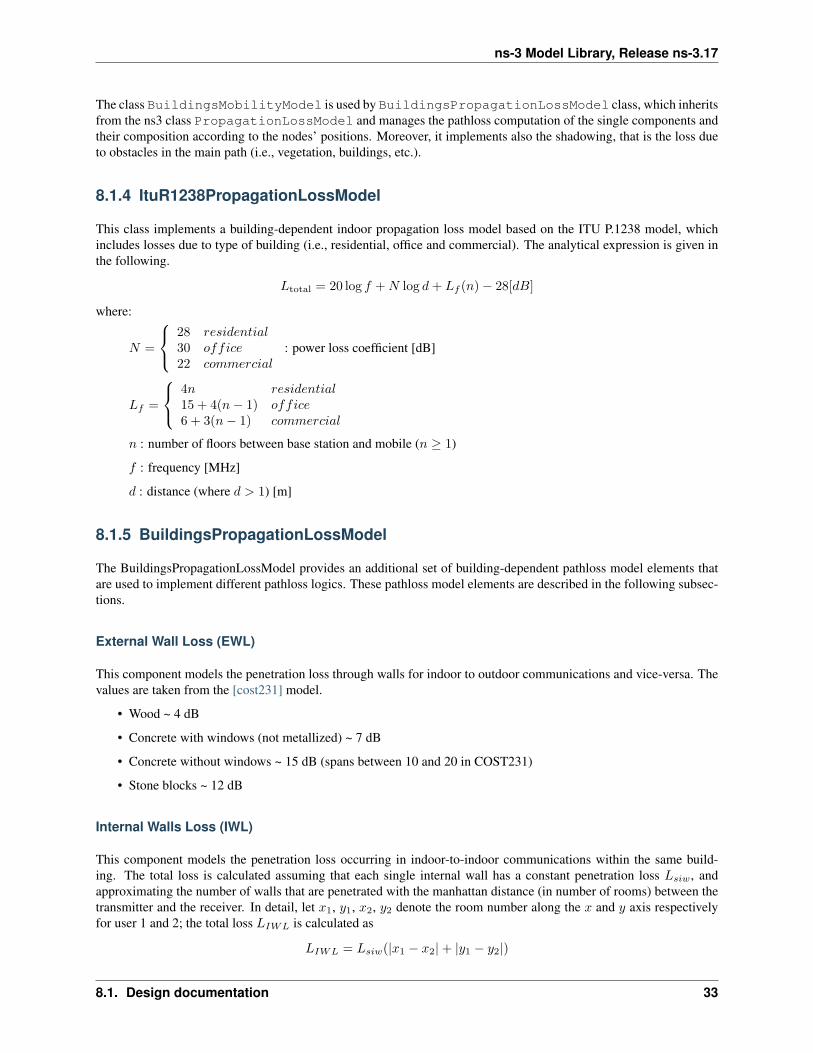
This class implements a building-dependent indoor propagation loss model based on the ITU P.1238 model, whichincludes losses due to type of building (i.e., residential, office and commercial). The analytical expression is given inthe following.
Ltotal = 20 log f +N log d+ Lf (n)− 28[dB]
where:
N =
28 residential30 office22 commercial
: power loss coefficient [dB]
Lf =
4n residential15 + 4(n− 1) office6 + 3(n− 1) commercial
n : number of floors between base station and mobile (n ≥ 1)
f : frequency [MHz]
d : distance (where d > 1) [m]
8.1.5 BuildingsPropagationLossModel
The BuildingsPropagationLossModel provides an additional set of building-dependent pathloss model elements thatare used to implement different pathloss logics. These pathloss model elements are described in the following subsec-tions.
External Wall Loss (EWL)
This component models the penetration loss through walls for indoor to outdoor communications and vice-versa. Thevalues are taken from the [cost231] model.
• Wood ~ 4 dB
• Concrete with windows (not metallized) ~ 7 dB
• Concrete without windows ~ 15 dB (spans between 10 and 20 in COST231)
• Stone blocks ~ 12 dB
Internal Walls Loss (IWL)
This component models the penetration loss occurring in indoor-to-indoor communications within the same build-ing. The total loss is calculated assuming that each single internal wall has a constant penetration loss Lsiw, andapproximating the number of walls that are penetrated with the manhattan distance (in number of rooms) between thetransmitter and the receiver. In detail, let x1, y1, x2, y2 denote the room number along the x and y axis respectivelyfor user 1 and 2; the total loss LIWL is calculated as
LIWL = Lsiw(|x1 − x2|+ |y1 − y2|)
8.1. Design documentation 33
ns-3 Model Library, Release ns-3.17
Height Gain Model (HG)
This component model the gain due to the fact that the transmitting device is on a floor above the ground. In theliterature [turkmani] this gain has been evaluated as about 2 dB per floor. This gain can be applied to all the indoor tooutdoor communications and vice-versa.
Shadowing Model
The shadowing is modeled according to a log-normal distribution with variable standard deviation as function of theconnection characteristics. In the implementation we considered three main possible scenarios which correspond tothree standard deviations (i.e., the mean is always 0), in detail:
• outdoor (m_shadowingSigmaOutdoor, defaul value of 7 dB)→ XO ∼ N(µO, σ2O).
• indoor (m_shadowingSigmaIndoor, defaul value of 10 dB)→ XI ∼ N(µI, σ2I ).
• external walls penetration (m_shadowingSigmaExtWalls, default value 5 dB)→ XW ∼ N(µW, σ2W)
The simulator generates a shadowing value per each active link according to nodes’ position the first time the linkis used for transmitting. In case of transmissions from outdoor nodes to indoor ones, and vice-versa, the standarddeviation (σIO) has to be calculated as the square root of the sum of the quadratic values of the standard deviatio incase of outdoor nodes and the one for the external walls penetration. This is due to the fact that that the componentsproducing the shadowing are independent of each other; therefore, the variance of a distribution resulting from thesum of two independent normal ones is the sum of the variances.
X ∼ N(µ, σ2) and Y ∼ N(ν, τ2)
Z = X + Y ∼ Z(µ+ ν, σ2 + τ2)
⇒ σIO =√σ2
O + σ2W
8.1.6 Pathloss logics
In the following we describe the different pathloss logic that are implemented by inheriting from BuildingsPropaga-tionLossModel.
HybridBuildingsPropagationLossModel
The HybridBuildingsPropagationLossModel pathloss model included is obtained through a combinationof several well known pathloss models in order to mimic different outdoor and indoor scenarios, as well as indoor-to-outdoor and outdoor-to-indoor scenarios. In detail, the class HybridBuildingsPropagationLossModelintegrates the following pathloss models:
• OkumuraHataPropagationLossModel (OH) (at frequencies > 2.3 GHz substituted byKun2600MhzPropagationLossModel)
• ItuR1411LosPropagationLossModel and ItuR1411NlosOverRooftopPropagationLossModel (I1411)
• ItuR1238PropagationLossModel (I1238)
• the pathloss elements of the BuildingsPropagationLossModel (EWL, HG, IWL)
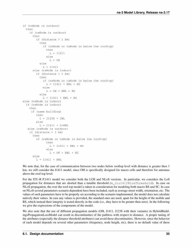
The following pseudo-code illustrates how the different pathloss model elements described above are integrated inHybridBuildingsPropagationLossModel:
34 Chapter 8. Buildings Module
ns-3 Model Library, Release ns-3.17
if (txNode is outdoor)thenif (rxNode is outdoor)
thenif (distance > 1 km)then
if (rxNode or txNode is below the rooftop)thenL = I1411
elseL = OH
elseL = I1411
else (rxNode is indoor)if (distance > 1 km)thenif (rxNode or txNode is below the rooftop)L = I1411 + EWL + HG
elseL = OH + EWL + HG
elseL = I1411 + EWL + HG
else (txNode is indoor)if (rxNode is indoor)thenif (same building)
thenL = I1238 + IWL
elseL = I1411 + 2*EWL
else (rxNode is outdoor)if (distance > 1 km)
thenif (rxNode or txNode is below the rooftop)
thenL = I1411 + EWL + HG
elseL = OH + EWL + HG
elseL = I1411 + EWL
We note that, for the case of communication between two nodes below rooftop level with distance is greater then 1km, we still consider the I1411 model, since OH is specifically designed for macro cells and therefore for antennasabove the roof-top level.
For the ITU-R P.1411 model we consider both the LOS and NLoS versions. In particular, we considers the LoSpropagation for distances that are shorted than a tunable threshold (m_itu1411NlosThreshold). In case onNLoS propagation, the over the roof-top model is taken in consideration for modeling both macro BS and SC. In caseon NLoS several parameters scenario dependent have been included, such as average street width, orientation, etc. Thevalues of such parameters have to be properly set according to the scenario implemented, the model does not calculatenatively their values. In case any values is provided, the standard ones are used, apart for the height of the mobile andBS, which instead their integrity is tested directly in the code (i.e., they have to be greater then zero). In the followingwe give the expressions of the components of the model.
We also note that the use of different propagation models (OH, I1411, I1238 with their variants) in HybridBuild-ingsPropagationLossModel can result in discontinuities of the pathloss with respect to distance. A proper tuning ofthe attributes (especially the distance threshold attributes) can avoid these discontinuities. However, since the behaviorof each model depends on several other parameters (frequency, node heigth, etc), there is no default value of these
8.1. Design documentation 35
ns-3 Model Library, Release ns-3.17
thresholds that can avoid the discontinuities in all possible configurations. Hence, an appropriate tuning of theseparameters is left to the user.
OhBuildingsPropagationLossModel
The OhBuildingsPropagationLossModel class has been created as a simple means to solve the discontinuityproblems of HybridBuildingsPropagationLossModel without doing scenario-specific parameter tuning.The solution is to use only one propagation loss model (i.e., Okumura Hata), while retaining the structure of thepathloss logic for the calculation of other path loss components (such as wall penetration losses). The result is a modelthat is free of discontinuities (except those due to walls), but that is less realistic overall for a generic scenario withbuildings and outdoor/indoor users, e.g., because Okumura Hata is not suitable neither for indoor communications norfor outdoor communications below rooftop level.
In detail, the class OhBuildingsPropagationLossModel integrates the following pathloss models:
• OkumuraHataPropagationLossModel (OH)
• the pathloss elements of the BuildingsPropagationLossModel (EWL, HG, IWL)
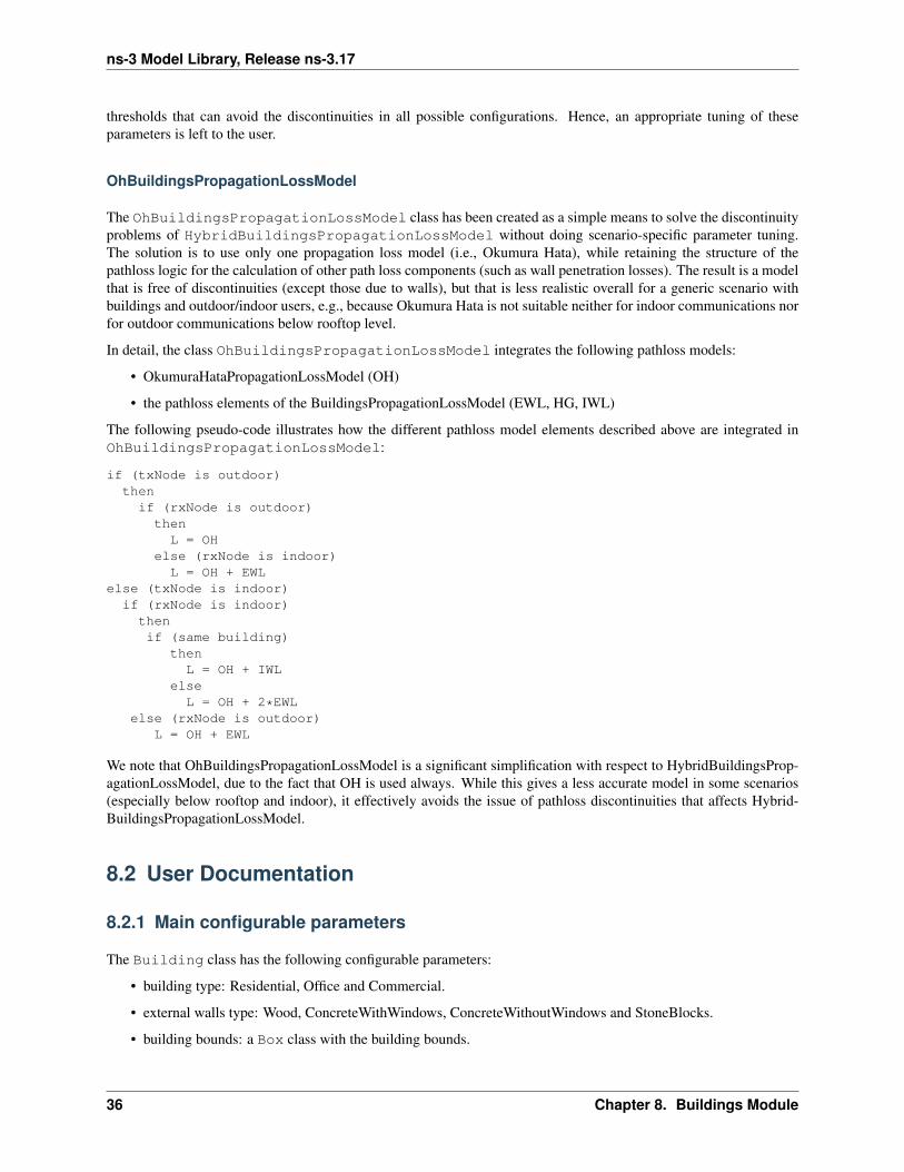
The following pseudo-code illustrates how the different pathloss model elements described above are integrated inOhBuildingsPropagationLossModel:
if (txNode is outdoor)thenif (rxNode is outdoor)
thenL = OH
else (rxNode is indoor)L = OH + EWL
else (txNode is indoor)if (rxNode is indoor)thenif (same building)
thenL = OH + IWL
elseL = OH + 2*EWL
else (rxNode is outdoor)L = OH + EWL
We note that OhBuildingsPropagationLossModel is a significant simplification with respect to HybridBuildingsProp-agationLossModel, due to the fact that OH is used always. While this gives a less accurate model in some scenarios(especially below rooftop and indoor), it effectively avoids the issue of pathloss discontinuities that affects Hybrid-BuildingsPropagationLossModel.
8.2 User Documentation
8.2.1 Main configurable parameters
The Building class has the following configurable parameters:
• building type: Residential, Office and Commercial.
• external walls type: Wood, ConcreteWithWindows, ConcreteWithoutWindows and StoneBlocks.
• building bounds: a Box class with the building bounds.
36 Chapter 8. Buildings Module
ns-3 Model Library, Release ns-3.17
• number of floors.
• number of rooms in x-axis and y-axis (rooms can be placed only in a grid way).
The BuildingMobilityLossModel parameter configurable with the ns3 attribute system is represented by thebound (string Bounds) of the simulation area by providing a Box class with the area bounds. Moreover, by means ofits methos the following parameters can be configured:
• the number of floor the node is placed (default 0).
• the position in the rooms grid.
The BuildingPropagationLossModel class has the following configurable parameters configurable with theattribute system:
• Frequency: reference frequency (default 2160 MHz), note that by setting the frequency the wavelength is setaccordingly automatically and viceversa).
• Lambda: the wavelength (0.139 meters, considering the above frequency).
• ShadowSigmaOutdoor: the standard deviation of the shadowing for outdoor nodes (defaul 7.0).
• ShadowSigmaIndoor: the standard deviation of the shadowing for indoor nodes (default 8.0).
• ShadowSigmaExtWalls: the standard deviation of the shadowing due to external walls penetration foroutdoor to indoor communications (default 5.0).
• RooftopLevel: the level of the rooftop of the building in meters (default 20 meters).
• Los2NlosThr: the value of distance of the switching point between line-of-sigth and non-line-of-sight prop-agation model in meters (default 200 meters).
• ITU1411DistanceThr: the value of distance of the switching point between short range (ITU 1211) com-munications and long range (Okumura Hata) in meters (default 200 meters).
• MinDistance: the minimum distance in meters between two nodes for evaluating the pathloss (consideredneglictible before this threshold) (default 0.5 meters).
• Environment: the environment scenario among Urban, SubUrban and OpenAreas (default Urban).
• CitySize: the dimension of the city among Small, Medium, Large (default Large).
In order to use the hybrid mode, the class to be used is the HybridBuildingMobilityLossModel, which allowsthe selection of the proper pathloss model according to the pathloss logic presented in the design chapter. However,this solution has the problem that the pathloss model switching points might present discontinuities due to the differentcharacteristics of the model. This implies that according to the specific scenario, the threshold used for switching haveto be properly tuned. The simple OhBuildingMobilityLossModel overcome this problem by using only theOkumura Hata model and the wall penetration losses.
8.3 Testing Documentation
8.3.1 Overview
To test and validate the ns-3 Building Pathloss module, some test suites is provided which are integrated with the ns-3test framework. To run them, you need to have configured the build of the simulator in this way:
./waf configure --enable-tests --enable-modules=buildings
./test.py
8.3. Testing Documentation 37

ns-3 Model Library, Release ns-3.17
The above will run not only the test suites belonging to the buildings module, but also those belonging to all the otherns-3 modules on which the buildings module depends. See the ns-3 manual for generic information on the testingframework.
You can get a more detailed report in HTML format in this way:
./test.py -w results.html
After the above command has run, you can view the detailed result for each test by opening the file results.htmlwith a web browser.
You can run each test suite separately using this command:
./test.py -s test-suite-name
For more details about test.py and the ns-3 testing framework, please refer to the ns-3 manual.
8.3.2 Description of the test suites
BuildingsHelper test
The test suite buildings-helper checks that the method BuildingsHelper::MakeAllInstancesConsistent() works properly, i.e., that the BuildingsHelper is successful in locating if nodes are outdoor or indoor, and if indoorthat they are located in the correct building, room and floor. Several test cases are provided with different buildings(having different size, position, rooms and floors) and different node positions. The test passes if each every node islocated correctly.
BuildingPositionAllocator test
The test suite building-position-allocator feature two test cases that check that respectively Random-RoomPositionAllocator and SameRoomPositionAllocator work properly. Each test cases involves a single 2x3x2room building (total 12 rooms) at known coordinates and respectively 24 and 48 nodes. Both tests check that thenumber of nodes allocated in each room is the expected one and that the position of the nodes is also correct.
Buildings Pathloss tests
The test suite buildings-pathloss-model provides different unit tests that compare the expected results ofthe buildings pathloss module in specific scenarios with pre calculated values obtained offline with an Octave script(test/reference/buildings-pathloss.m). The tests are considered passed if the two values are equal up to a tolerance of0.1, which is deemed appropriate for the typical usage of pathloss values (which are in dB).
In the following we detailed the scenarios considered, their selection has been done for covering the wide set ofpossible pathloss logic combinations. The pathloss logic results therefore implicitly tested.
Test #1 Okumura Hata
In this test we test the standard Okumura Hata model; therefore both eNB and UE are placed outside at a distanceof 2000 m. The frequency used is the E-UTRA band #5, which correspond to 869 MHz (see table 5.5-1 of 36.101).The test includes also the validation of the areas extensions (i.e., urban, suburban and open-areas) and of the city size(small, medium and large).
38 Chapter 8. Buildings Module
ns-3 Model Library, Release ns-3.17
Test #2 COST231 Model
This test is aimed at validating the COST231 model. The test is similar to the Okumura Hata one, except that thefrequency used is the EUTRA band #1 (2140 MHz) and that the test can be performed only for large and small citiesin urban scenarios due to model limitations.
Test #3 2.6 GHz model
This test validates the 2.6 GHz Kun model. The test is similar to Okumura Hata one except that the frequency is theEUTRA band #7 (2620 MHz) and the test can be performed only in urban scenario.
Test #4 ITU1411 LoS model
This test is aimed at validating the ITU1411 model in case of line of sight within street canyons transmissions. In thiscase the UE is placed at 100 meters far from the eNB, since the threshold for switching between LoS and NLoS is leftto default one (i.e., 200 m.).
Test #5 ITU1411 NLoS model
This test is aimed at validating the ITU1411 model in case of non line of sight over the rooftop transmissions. In thiscase the UE is placed at 900 meters far from the eNB, in order to be above the threshold for switching between LoSand NLoS is left to default one (i.e., 200 m.).
Test #6 ITUP1238 model
This test is aimed at validating the ITUP1238 model in case of indoor transmissions. In this case both the UE and theeNB are placed in a residential building with walls made of concrete with windows. Ue is placed at the second floorand distances 30 meters far from the eNB, which is placed at the first floor.
Test #7 Outdoor -> Indoor with Okumura Hata model
This test validates the outdoor to indoor transmissions for large distances. In this case the UE is placed in a residentialbuilding with wall made of concrete with windows and distances 2000 meters from the outdoor eNB.
Test #8 Outdoor -> Indoor with ITU1411 model
This test validates the outdoor to indoor transmissions for short distances. In this case the UE is placed in a residentialbuilding with walls made of concrete with windows and distances 100 meters from the outdoor eNB.
Test #9 Indoor -> Outdoor with ITU1411 model
This test validates the outdoor to indoor transmissions for very short distances. In this case the eNB is placed in thesecond floor of a residential building with walls made of concrete with windows and distances 100 meters from theoutdoor UE (i.e., LoS communication). Therefore the height gain has to be included in the pathloss evaluation.
8.3. Testing Documentation 39
ns-3 Model Library, Release ns-3.17
Test #10 Indoor -> Outdoor with ITU1411 model
This test validates the outdoor to indoor transmissions for short distances. In this case the eNB is placed in the secondfloor of a residential building with walls made of concrete with windows and distances 500 meters from the outdoorUE (i.e., NLoS communication). Therefore the height gain has to be included in the pathloss evaluation.
Buildings Shadowing Test
The test suite buildings-shadowing-test is a unit test intended to verify the statistics distribution charac-teristics of the shadowing are the one expected. The shadowing is modeled according to a normal distribution withmean µ = 0 and variable standard deviation σ, according to models commonly used in literature. The test gen-erates 10,000 samples of shadowing by subtracting the deterministic component from the total loss returned by theBuildingPathlossModel. The mean and variance of the shadowing samples are then used to verify whether the99% confidence interval is respected by the sequence generated by the simulator.
8.4 References
40 Chapter 8. Buildings Module
CHAPTER
NINE
CLICK MODULAR ROUTERINTEGRATION
Click is a software architecture for building configurable routers. By using different combinations of packet processingunits called elements, a Click router can be made to perform a specific kind of functionality. This flexibility providesa good platform for testing and experimenting with different protocols.
9.1 Model Description
The source code for the Click model lives in the directory src/click.
9.1.1 Design
ns-3’s design is well suited for an integration with Click due to the following reasons:
• Packets in ns-3 are serialised/deserialised as they move up/down the stack. This allows ns-3 packets to be passedto and from Click as they are.
• This also means that any kind of ns-3 traffic generator and transport should work easily on top of Click.
• By striving to implement click as an Ipv4RoutingProtocol instance, we can avoid significant changes to the LLand MAC layer of the ns-3 code.
The design goal was to make the ns-3-click public API simple enough such that the user needs to merely add anIpv4ClickRouting instance to the node, and inform each Click node of the Click configuration file (.click file) that it isto use.
This model implements the interface to the Click Modular Router and provides the Ipv4ClickRouting class to allow anode to use Click for external routing. Unlike normal Ipv4RoutingProtocol sub types, Ipv4ClickRouting doesn’t use aRouteInput() method, but instead, receives a packet on the appropriate interface and processes it accordingly. Note thatyou need to have a routing table type element in your Click graph to use Click for external routing. This is needed bythe RouteOutput() function inherited from Ipv4RoutingProtocol. Furthermore, a Click based node uses a different kindof L3 in the form of Ipv4L3ClickProtocol, which is a trimmed down version of Ipv4L3Protocol. Ipv4L3ClickProtocolpasses on packets passing through the stack to Ipv4ClickRouting for processing.
Developing a Simulator API to allow ns-3 to interact with Click
Much of the API is already well defined, which allows Click to probe for information from the simulator (like a Node’sID, an Interface ID and so forth). By retaining most of the methods, it should be possible to write new implementationsspecific to ns-3 for the same functionality.
41
ns-3 Model Library, Release ns-3.17
Hence, for the Click integration with ns-3, a class named Ipv4ClickRouting will handle the interaction with Click. Thecode for the same can be found in src/click/model/ipv4-click-routing.{cc,h}.
Packet hand off between ns-3 and Click
There are four kinds of packet hand-offs that can occur between ns-3 and Click.
• L4 to L3
• L3 to L4
• L3 to L2
• L2 to L3
To overcome this, we implement Ipv4L3ClickProtocol, a stripped down version of Ipv4L3Protocol.Ipv4L3ClickProtocol passes packets to and from Ipv4ClickRouting appropriately to perform routing.
9.1.2 Scope and Limitations
• In its current state, the NS-3 Click Integration is limited to use only with L3, leaving NS-3 to handle L2. We arecurrently working on adding Click MAC support as well. See the usage section to make sure that you designyour Click graphs accordingly.
• Furthermore, ns-3-click will work only with userlevel elements. The complete list of elements are available athttp://read.cs.ucla.edu/click/elements. Elements that have ‘all’, ‘userlevel’ or ‘ns’ mentioned beside them maybe used.
• As of now, the ns-3 interface to Click is Ipv4 only. We will be adding Ipv6 support in the future.
9.1.3 References
• Eddie Kohler, Robert Morris, Benjie Chen, John Jannotti, and M. Frans Kaashoek. The click modular router.ACM Transactions on Computer Systems 18(3), August 2000, pages 263-297.
• Lalith Suresh P., and Ruben Merz. Ns-3-click: click modular router integration for ns-3. In Proc. of 3rdInternational ICST Workshop on NS-3 (WNS3), Barcelona, Spain. March, 2011.
• Michael Neufeld, Ashish Jain, and Dirk Grunwald. Nsclick: bridging network simulation and deployment.MSWiM ‘02: Proceedings of the 5th ACM international workshop on Modeling analysis and simulation ofwireless and mobile systems, 2002, Atlanta, Georgia, USA. http://doi.acm.org/10.1145/570758.570772
9.2 Usage
9.2.1 Building Click
The first step is to clone Click from the github repository and build it:
$: git clone https://github.com/kohler/click$: cd click/$: ./configure --disable-linuxmodule --enable-nsclick --enable-wifi$: make
42 Chapter 9. Click Modular Router Integration
ns-3 Model Library, Release ns-3.17
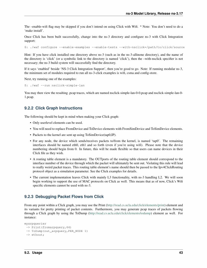
The –enable-wifi flag may be skipped if you don’t intend on using Click with Wifi. * Note: You don’t need to do a‘make install’.
Once Click has been built successfully, change into the ns-3 directory and configure ns-3 with Click Integrationsupport:
$: ./waf configure --enable-examples --enable-tests --with-nsclick=/path/to/click/source
Hint: If you have click installed one directory above ns-3 (such as in the ns-3-allinone directory), and the name ofthe directory is ‘click’ (or a symbolic link to the directory is named ‘click’), then the –with-nsclick specifier is notnecessary; the ns-3 build system will successfully find the directory.
If it says ‘enabled’ beside ‘NS-3 Click Integration Support’, then you’re good to go. Note: If running modular ns-3,the minimum set of modules required to run all ns-3-click examples is wifi, csma and config-store.
Next, try running one of the examples:
$: ./waf --run nsclick-simple-lan
You may then view the resulting .pcap traces, which are named nsclick-simple-lan-0-0.pcap and nsclick-simple-lan-0-1.pcap.
9.2.2 Click Graph Instructions
The following should be kept in mind when making your Click graph:
• Only userlevel elements can be used.
• You will need to replace FromDevice and ToDevice elements with FromSimDevice and ToSimDevice elements.
• Packets to the kernel are sent up using ToSimDevice(tap0,IP).
• For any node, the device which sends/receives packets to/from the kernel, is named ‘tap0’. The remaininginterfaces should be named eth0, eth1 and so forth (even if you’re using wifi). Please note that the devicenumbering should begin from 0. In future, this will be made flexible so that users can name devices in theirClick file as they wish.
• A routing table element is a mandatory. The OUTports of the routing table element should correspond to theinterface number of the device through which the packet will ultimately be sent out. Violating this rule will leadto really weird packet traces. This routing table element’s name should then be passed to the Ipv4ClickRoutingprotocol object as a simulation parameter. See the Click examples for details.
• The current implementation leaves Click with mainly L3 functionality, with ns-3 handling L2. We will soonbegin working to support the use of MAC protocols on Click as well. This means that as of now, Click’s Wifispecific elements cannot be used with ns-3.
9.2.3 Debugging Packet Flows from Click
From any point within a Click graph, you may use the Print (http://read.cs.ucla.edu/click/elements/print) element andits variants for pretty printing of packet contents. Furthermore, you may generate pcap traces of packets flowingthrough a Click graph by using the ToDump (http://read.cs.ucla.edu/click/elements/todump) element as well. Forinstance:
myarpquerier-> Print(fromarpquery,64)-> ToDump(out_arpquery,PER_NODE 1)-> ethout;
9.2. Usage 43
ns-3 Model Library, Release ns-3.17
and ...will print the contents of packets that flow out of the ArpQuerier, then generate a pcap trace file which will havea suffix ‘out_arpquery’, for each node using the Click file, before pushing packets onto ‘ethout’.
9.2.4 Helper
To have a node run Click, the easiest way would be to use the ClickInternetStackHelper class in your simulation script.For instance:
ClickInternetStackHelper click;click.SetClickFile (myNodeContainer, "nsclick-simple-lan.click");click.SetRoutingTableElement (myNodeContainer, "u/rt");click.Install (myNodeContainer);
The example scripts inside src/click/examples/ demonstrate the use of Clickbased nodes in different scenarios. The helper source can be found insidesrc/click/helper/click-internet-stack-helper.{h,cc}
9.2.5 Examples
The following examples have been written, which can be found in src/click/examples/:
• nsclick-simple-lan.cc and nsclick-raw-wlan.cc: A Click based node communicating with a normal ns-3 nodewithout Click, using Csma and Wifi respectively. It also demonstrates the use of TCP on top of Click, somethingwhich the original nsclick implementation for NS-2 couldn’t achieve.
• nsclick-udp-client-server-csma.cc and nsclick-udp-client-server-wifi.cc: A 3 node LAN (Csma and Wifi respec-tively) wherein 2 Click based nodes run a UDP client, that sends packets to a third Click based node running aUDP server.
• nsclick-routing.cc: One Click based node communicates to another via a third node that acts as an IP router(using the IP router Click configuration). This demonstrates routing using Click.
Scripts are available within <click-dir>/conf/ that allow you to generate Click files for some common sce-narios. The IP Router used in nsclick-routing.cc was generated from the make-ip-conf.pl file and slightlyadapted to work with ns-3-click.
9.3 Validation
This model has been tested as follows:
• Unit tests have been written to verify the internals of Ipv4ClickRouting. This can be found insrc/click/ipv4-click-routing-test.cc. These tests verify whether the methods insideIpv4ClickRouting which deal with Device name to ID, IP Address from device name and Mac Address fromdevice name bindings work as expected.
• The examples have been used to test Click with actual simulation scenarios. These can be found insrc/click/examples/. These tests cover the following: the use of different kinds of transports on topof Click, TCP/UDP, whether Click nodes can communicate with non-Click based nodes, whether Click nodescan communicate with each other, using Click to route packets using static routing.
• Click has been tested with Csma, Wifi and Point-to-Point devices. Usage instructions are available in the pre-ceding section.
44 Chapter 9. Click Modular Router Integration
CHAPTER
TEN
CSMA NETDEVICE
This is the introduction to CSMA NetDevice chapter, to complement the Csma model doxygen.
10.1 Overview of the CSMA model
The ns-3 CSMA device models a simple bus network in the spirit of Ethernet. Although it does not model any realphysical network you could ever build or buy, it does provide some very useful functionality.
Typically when one thinks of a bus network Ethernet or IEEE 802.3 comes to mind. Ethernet uses CSMA/CD (Car-rier Sense Multiple Access with Collision Detection with exponentially increasing backoff to contend for the sharedtransmission medium. The ns-3 CSMA device models only a portion of this process, using the nature of the globallyavailable channel to provide instantaneous (faster than light) carrier sense and priority-based collision “avoidance.”Collisions in the sense of Ethernet never happen and so the ns-3 CSMA device does not model collision detection, norwill any transmission in progress be “jammed.”
10.1.1 CSMA Layer Model
There are a number of conventions in use for describing layered communications architectures in the literature and intextbooks. The most common layering model is the ISO seven layer reference model. In this view the CsmaNetDeviceand CsmaChannel pair occupies the lowest two layers – at the physical (layer one), and data link (layer two) positions.Another important reference model is that specified by RFC 1122, “Requirements for Internet Hosts – CommunicationLayers.” In this view the CsmaNetDevice and CsmaChannel pair occupies the lowest layer – the link layer. There isalso a seemingly endless litany of alternative descriptions found in textbooks and in the literature. We adopt the namingconventions used in the IEEE 802 standards which speak of LLC, MAC, MII and PHY layering. These acronyms aredefined as:
• LLC: Logical Link Control;
• MAC: Media Access Control;
• MII: Media Independent Interface;
• PHY: Physical Layer.
In this case the LLC and MAC are sublayers of the OSI data link layer and the MII and PHY are sublayers of the OSIphysical layer.
The “top” of the CSMA device defines the transition from the network layer to the data link layer. This transition isperformed by higher layers by calling either CsmaNetDevice::Send or CsmaNetDevice::SendFrom.
In contrast to the IEEE 802.3 standards, there is no precisely specified PHY in the CSMA model in the sense of wiretypes, signals or pinouts. The “bottom” interface of the CsmaNetDevice can be thought of as as a kind of Media
45
ns-3 Model Library, Release ns-3.17
Independent Interface (MII) as seen in the “Fast Ethernet” (IEEE 802.3u) specifications. This MII interface fits into acorresponding media independent interface on the CsmaChannel. You will not find the equivalent of a 10BASE-T ora 1000BASE-LX PHY.
The CsmaNetDevice calls the CsmaChannel through a media independent interface. There is a method defined to tellthe channel when to start “wiggling the wires” using the method CsmaChannel::TransmitStart, and a method to tellthe channel when the transmission process is done and the channel should begin propagating the last bit across the“wire”: CsmaChannel::TransmitEnd.
When the TransmitEnd method is executed, the channel will model a single uniform signal propagation delay in themedium and deliver copes of the packet to each of the devices attached to the packet via the CsmaNetDevice::Receivemethod.
There is a “pin” in the device media independent interface corresponding to “COL” (collision). The state of the channelmay be sensed by calling CsmaChannel::GetState. Each device will look at this “pin” before starting a send and willperform appropriate backoff operations if required.
Properly received packets are forwarded up to higher levels from the CsmaNetDevice via a callback mechanism.The callback function is initialized by the higher layer (when the net device is attached) using CsmaNetDe-vice::SetReceiveCallback and is invoked upon “proper” reception of a packet by the net device in order to forwardthe packet up the protocol stack.
10.2 CSMA Channel Model
The class CsmaChannel models the actual transmission medium. There is no fixed limit for the number of devicesconnected to the channel. The CsmaChannel models a data rate and a speed-of-light delay which can be accessed viathe attributes “DataRate” and “Delay” respectively. The data rate provided to the channel is used to set the data ratesused by the transmitter sections of the CSMA devices connected to the channel. There is no way to independently setdata rates in the devices. Since the data rate is only used to calculate a delay time, there is no limitation (other thanby the data type holding the value) on the speed at which CSMA channels and devices can operate; and no restrictionbased on any kind of PHY characteristics.
The CsmaChannel has three states, IDLE, TRANSMITTING and PROPAGATING. These three states are “seen” in-stantaneously by all devices on the channel. By this we mean that if one device begins or ends a simulated transmission,all devices on the channel are immediately aware of the change in state. There is no time during which one device maysee an IDLE channel while another device physically further away in the collision domain may have begun transmit-ting with the associated signals not propagated down the channel to other devices. Thus there is no need for collisiondetection in the CsmaChannel model and it is not implemented in any way.
We do, as the name indicates, have a Carrier Sense aspect to the model. Since the simulator is single threaded, accessto the common channel will be serialized by the simulator. This provides a deterministic mechanism for contendingfor the channel. The channel is allocated (transitioned from state IDLE to state TRANSMITTING) on a first-comefirst-served basis. The channel always goes through a three state process::
IDLE -> TRANSMITTING -> PROPAGATING -> IDLE
The TRANSMITTING state models the time during which the source net device is actually wiggling the signals on thewire. The PROPAGATING state models the time after the last bit was sent, when the signal is propagating down thewire to the “far end.”
The transition to the TRANSMITTING state is driven by a call to CsmaChannel::TransmitStart which is called bythe net device that transmits the packet. It is the responsibility of that device to end the transmission with a call toCsmaChannel::TransmitEnd at the appropriate simulation time that reflects the time elapsed to put all of the packetbits on the wire. When TransmitEnd is called, the channel schedules an event corresponding to a single speed-of-light delay. This delay applies to all net devices on the channel identically. You can think of a symmetrical hub inwhich the packet bits propagate to a central location and then back out equal length cables to the other devices on the
46 Chapter 10. CSMA NetDevice
ns-3 Model Library, Release ns-3.17
channel. The single “speed of light” delay then corresponds to the time it takes for: 1) a signal to propagate from oneCsmaNetDevice through its cable to the hub; plus 2) the time it takes for the hub to forward the packet out a port; plus3) the time it takes for the signal in question to propagate to the destination net device.
The CsmaChannel models a broadcast medium so the packet is delivered to all of the devices on the channel (includingthe source) at the end of the propagation time. It is the responsibility of the sending device to determine whether ornot it receives a packet broadcast over the channel.
The CsmaChannel provides following Attributes:
• DataRate: The bitrate for packet transmission on connected devices;
• Delay: The speed of light transmission delay for the channel.
10.3 CSMA Net Device Model
The CSMA network device appears somewhat like an Ethernet device. The CsmaNetDevice provides following At-tributes:
• Address: The Mac48Address of the device;
• SendEnable: Enable packet transmission if true;
• ReceiveEnable: Enable packet reception if true;
• EncapsulationMode: Type of link layer encapsulation to use;
• RxErrorModel: The receive error model;
• TxQueue: The transmit queue used by the device;
• InterframeGap: The optional time to wait between “frames”;
• Rx: A trace source for received packets;
• Drop: A trace source for dropped packets.
The CsmaNetDevice supports the assignment of a “receive error model.” This is an ErrorModel object that is used tosimulate data corruption on the link.
Packets sent over the CsmaNetDevice are always routed through the transmit queue to provide a trace hook for packetssent out over the network. This transmit queue can be set (via attribute) to model different queuing strategies.
Also configurable by attribute is the encapsulation method used by the device. Every packet gets an EthernetHeaderthat includes the destination and source MAC addresses, and a length/type field. Every packet also gets an Ethernet-Trailer which includes the FCS. Data in the packet may be encapsulated in different ways.
By default, or by setting the “EncapsulationMode” attribute to “Dix”, the encapsulation is according to the DEC,Intel, Xerox standard. This is sometimes called EthernetII framing and is the familiar destination MAC, source MAC,EtherType, Data, CRC format.
If the “EncapsulationMode” attribute is set to “Llc”, the encapsulation is by LLC SNAP. In this case, a SNAP headeris added that contains the EtherType (IP or ARP).
The other implemented encapsulation modes are IP_ARP (set “EncapsulationMode” to “IpArp”) in which the lengthtype of the Ethernet header receives the protocol number of the packet; or ETHERNET_V1 (set “EncapsulationMode”to “EthernetV1”) in which the length type of the Ethernet header receives the length of the packet. A “Raw” encapsu-lation mode is defined but not implemented – use of the RAW mode results in an assertion.
Note that all net devices on a channel must be set to the same encapsulation mode for correct results. The encapsulationmode is not sensed at the receiver.
10.3. CSMA Net Device Model 47
ns-3 Model Library, Release ns-3.17
The CsmaNetDevice implements a random exponential backoff algorithm that is executed if the channel is determinedto be busy (TRANSMITTING or PPROPAGATING) when the device wants to start propagating. This results in arandom delay of up to pow (2, retries) - 1 microseconds before a retry is attempted. The default maximum number ofretries is 1000.
10.4 Using the CsmaNetDevice
The CSMA net devices and channels are typically created and configured using the associated CsmaHelper object.The various ns-3 device helpers generally work in a similar way, and their use is seen in many of our example programs.
The conceptual model of interest is that of a bare computer “husk” into which you plug net devices. The bare computersare created using a NodeContainer helper. You just ask this helper to create as many computers (we call themNodes) as you need on your network::
NodeContainer csmaNodes;csmaNodes.Create (nCsmaNodes);
Once you have your nodes, you need to instantiate a CsmaHelper and set any attributes you may want to change.:
CsmaHelper csma;csma.SetChannelAttribute ("DataRate", StringValue ("100Mbps"));csma.SetChannelAttribute ("Delay", TimeValue (NanoSeconds (6560)));
csma.SetDeviceAttribute ("EncapsulationMode", StringValue ("Dix"));csma.SetDeviceAttribute ("FrameSize", UintegerValue (2000));
Once the attributes are set, all that remains is to create the devices and install them on the required nodes, and toconnect the devices together using a CSMA channel. When we create the net devices, we add them to a container toallow you to use them in the future. This all takes just one line of code.:
NetDeviceContainer csmaDevices = csma.Install (csmaNodes);
We recommend thinking carefully about changing these Attributes, since it can result in behavior that surprises users.We allow this because we believe flexibility is important. As an example of a possibly surprising effect of changingAttributes, consider the following:
The Mtu Attribute indicates the Maximum Transmission Unit to the device. This is the size of the largest ProtocolData Unit (PDU) that the device can send. This Attribute defaults to 1500 bytes and corresponds to a number foundin RFC 894, “A Standard for the Transmission of IP Datagrams over Ethernet Networks.” The number is actuallyderived from the maximum packet size for 10Base5 (full-spec Ethernet) networks – 1518 bytes. If you subtract DIXencapsulation overhead for Ethernet packets (18 bytes) you will end up with a maximum possible data size (MTU)of 1500 bytes. One can also find that the MTU for IEEE 802.3 networks is 1492 bytes. This is because LLC/SNAPencapsulation adds an extra eight bytes of overhead to the packet. In both cases, the underlying network hardware islimited to 1518 bytes, but the MTU is different because the encapsulation is different.
If one leaves the Mtu Attribute at 1500 bytes and changes the encapsulation mode Attribute to Llc, the result will be anetwork that encapsulates 1500 byte PDUs with LLC/SNAP framing resulting in packets of 1526 bytes. This wouldbe illegal in many networks, but we allow you do do this. This results in a simulation that quite subtly does not reflectwhat you might be expecting since a real device would balk at sending a 1526 byte packet.
There also exist jumbo frames (1500 < MTU <= 9000 bytes) and super-jumbo (MTU > 9000 bytes) frames thatare not officially sanctioned by IEEE but are available in some high-speed (Gigabit) networks and NICs. In theCSMA model, one could leave the encapsulation mode set to Dix, and set the Mtu to 64000 bytes – even though anassociated CsmaChannel DataRate was left at 10 megabits per second (certainly not Gigabit Ethernet). This wouldessentially model an Ethernet switch made out of vampire-tapped 1980s-style 10Base5 networks that support super-jumbo datagrams, which is certainly not something that was ever made, nor is likely to ever be made; however it isquite easy for you to configure.
48 Chapter 10. CSMA NetDevice

ns-3 Model Library, Release ns-3.17
Be careful about assumptions regarding what CSMA is actually modelling and how configuration (Attributes) mayallow you to swerve considerably away from reality.
10.5 CSMA Tracing
Like all ns-3 devices, the CSMA Model provides a number of trace sources. These trace sources can be hooked usingyour own custom trace code, or you can use our helper functions to arrange for tracing to be enabled on devices youspecify.
10.5.1 Upper-Level (MAC) Hooks
From the point of view of tracing in the net device, there are several interesting points to insert trace hooks. A con-vention inherited from other simulators is that packets destined for transmission onto attached networks pass througha single “transmit queue” in the net device. We provide trace hooks at this point in packet flow, which corresponds(abstractly) only to a transition from the network to data link layer, and call them collectively the device MAC hooks.
When a packet is sent to the CSMA net device for transmission it always passes through the transmit queue. Thetransmit queue in the CsmaNetDevice inherits from Queue, and therefore inherits three trace sources:
• An Enqueue operation source (see Queue::m_traceEnqueue);
• A Dequeue operation source (see Queue::m_traceDequeue);
• A Drop operation source (see Queue::m_traceDrop).
The upper-level (MAC) trace hooks for the CsmaNetDevice are, in fact, exactly these three trace sources on the singletransmit queue of the device.
The m_traceEnqueue event is triggered when a packet is placed on the transmit queue. This happens at the time thatCsmaNetDevice::Send or CsmaNetDevice::SendFrom is called by a higher layer to queue a packet for transmission.
The m_traceDequeue event is triggered when a packet is removed from the transmit queue. Dequeues from the trans-mit queue can happen in three situations: 1) If the underlying channel is idle when the CsmaNetDevice::Send orCsmaNetDevice::SendFrom is called, a packet is dequeued from the transmit queue and immediately transmitted; 2)If the underlying channel is idle, a packet may be dequeued and immediately transmitted in an internal TransmitCom-pleteEvent that functions much like a transmit complete interrupt service routine; or 3) from the random exponentialbackoff handler if a timeout is detected.
Case (3) implies that a packet is dequeued from the transmit queue if it is unable to be transmitted according to thebackoff rules. It is important to understand that this will appear as a Dequeued packet and it is easy to incorrectlyassume that the packet was transmitted since it passed through the transmit queue. In fact, a packet is actually droppedby the net device in this case. The reason for this behavior is due to the definition of the Queue Drop event. Them_traceDrop event is, by definition, fired when a packet cannot be enqueued on the transmit queue because it is full.This event only fires if the queue is full and we do not overload this event to indicate that the CsmaChannel is “full.”
10.5.2 Lower-Level (PHY) Hooks
Similar to the upper level trace hooks, there are trace hooks available at the lower levels of the net device. We callthese the PHY hooks. These events fire from the device methods that talk directly to the CsmaChannel.
The trace source m_dropTrace is called to indicate a packet that is dropped by the device. This happens in two cases:First, if the receive side of the net device is not enabled (see CsmaNetDevice::m_receiveEnable and the associatedattribute “ReceiveEnable”).
The m_dropTrace is also used to indicate that a packet was discarded as corrupt if a receive error model is used (seeCsmaNetDevice::m_receiveErrorModel and the associated attribute “ReceiveErrorModel”).
10.5. CSMA Tracing 49
ns-3 Model Library, Release ns-3.17
The other low-level trace source fires on reception of an accepted packet (see CsmaNetDevice::m_rxTrace). A packetis accepted if it is destined for the broadcast address, a multicast address, or to the MAC address assigned to the netdevice.
10.6 Summary
The ns3 CSMA model is a simplistic model of an Ethernet-like network. It supports a Carrier-Sense function andallows for Multiple Access to a shared medium. It is not physical in the sense that the state of the medium is instan-taneously shared among all devices. This means that there is no collision detection required in this model and noneis implemented. There will never be a “jam” of a packet already on the medium. Access to the shared channel is ona first-come first-served basis as determined by the simulator scheduler. If the channel is determined to be busy bylooking at the global state, a random exponential backoff is performed and a retry is attempted.
Ns-3 Attributes provide a mechanism for setting various parameters in the device and channel such as addresses,encapsulation modes and error model selection. Trace hooks are provided in the usual manner with a set of upper levelhooks corresponding to a transmit queue and used in ASCII tracing; and also a set of lower level hooks used in pcaptracing.
Although the ns-3 CsmaChannel and CsmaNetDevice does not model any kind of network you could build or buy, itdoes provide us with some useful functionality. You should, however, understand that it is explicitly not Ethernet orany flavor of IEEE 802.3 but an interesting subset.
50 Chapter 10. CSMA NetDevice
CHAPTER
ELEVEN
DSDV ROUTING
Destination-Sequenced Distance Vector (DSDV) routing protocol is a pro-active, table-driven routing protocol forMANETs developed by Charles E. Perkins and Pravin Bhagwat in 1994. It uses the hop count as metric in routeselection.
This model was developed by the ResiliNets research group at the University of Kansas. A paper on this model existsat this URL.
11.1 DSDV Routing Overview
DSDV Routing Table: Every node will maintain a table listing all the other nodes it has known either directly orthrough some neighbors. Every node has a single entry in the routing table. The entry will have information aboutthe node’s IP address, last known sequence number and the hop count to reach that node. Along with these details thetable also keeps track of the nexthop neighbor to reach the destination node, the timestamp of the last update receivedfor that node.
The DSDV update message consists of three fields, Destination Address, Sequence Number and Hop Count.
Each node uses 2 mechanisms to send out the DSDV updates. They are,
1. Periodic Updates Periodic updates are sent out after every m_periodicUpdateInterval(default:15s). In this up-date the node broadcasts out its entire routing table.
2. Trigger Updates Trigger Updates are small updates in-between the periodic updates. These updates are sentout whenever a node receives a DSDV packet that caused a change in its routing table. The original paperdid not clearly mention when for what change in the table should a DSDV update be sent out. The currentimplemntation sends out an update irrespective of the change in the routing table.
The updates are accepted based on the metric for a particular node. The first factor determinig the acceptance of anupdate is the sequence number. It has to accept the update if the sequence number of the update message is higherirrespective of the metric. If the update with same sequence number is received, then the update with least metric(hopCount) is given precedence.
In highly mobile scenarios, there is a high chance of route fluctuations, thus we have the concept of weighted settlingtime where an update with change in metric will not be advertised to neighbors. The node waits for the settling timeto make sure that it did not receive the update from its old neighbor before sending out that update.
The current implementation covers all the above features of DSDV. The current implementation also has a requestqueue to buffer packets that have no routes to destination. The default is set to buffer up to 5 packets per destination.
51

ns-3 Model Library, Release ns-3.17
11.2 References
Link to the Paper: http://portal.acm.org/citation.cfm?doid=190314.190336
52 Chapter 11. DSDV Routing
CHAPTER
TWELVE
DSR ROUTING
Dynamic Source Routing (DSR) protocol is a reactive routing protocol designed specifically for use in multi-hopwireless ad hoc networks of mobile nodes.
This model was developed by the ResiliNets research group at the University of Kansas.
12.1 DSR Routing Overview
This model implements the base specification of the Dynamic Source Routing (DSR) protocol. Implementation isbased on RFC4728.
DSR operates on a on-demand behavior. Therefore, our DSR model buffers all packets while a route request packet(RREQ) is disseminated. We implement a packet buffer in dsr-rsendbuff.cc. The packet queue implements garbagecollection of old packets and a queue size limit. When the packet is sent out from the send buffer, it will be queued inmaintenance buffer for next hop acknowledgment.
The maintenance buffer then buffers the already sent out packets and waits for the notification of packet delivery.Protocol operation strongly depends on broken link detection mechanism. We implement the three heuristics recom-mended based the RFC as follows:
First, we use link layer feedback when possible, which is also the fastest mechanism of these three to detect link errors.A link is considered to be broken if frame transmission results in a transmission failure for all retries. This mechanismis meant for active links and works much faster than in its absence. DSR is able to detect the link layer transmissionfailure and notify that as broken. Recalculation of routes will be triggered when needed. If user does not want to uselink layer acknowledgment, it can be tuned by setting “LinkAcknowledgment” attribute to false in “dsr-routing.cc”.
Second, passive acknowledgment should be used whenever possible. The node turns on “promiscuous” receive mode,in which it can receive packets not destined for itself, and when the node assures the delivery of that data packet to itsdestination, it cancels the passive acknowledgment timer.
Last, we use a network layer acknowledge scheme to notify the receipt of a packet. Route request packet will not beacknowledged or retransmitted.
The Route Cache implementation support garbage collection of old entries and state machine, as defined in the stan-dard. It implements as a STL map container. The key is the destination IP address.
DSR operates with direct access to IP header, and operates between network and transport layer. When packet is sentout from transport layer, it passes itself to DSR and DSR header is appended.
We have two caching mechanisms: path cache and link cache. The path cache saves the whole path in the cache. Thepaths are sorted based on the hop count, and whenever one path is not able to be used, we change to the next path.The link cache is a slightly better design in the sense that it uses different subpaths and uses Implemented Link Cacheusing Dijsktra algorithm, and this part is implemented by Song Luan <[email protected]>.
53
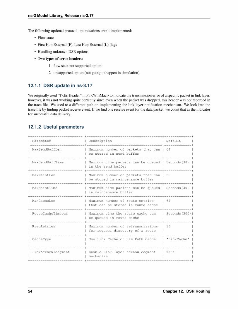
ns-3 Model Library, Release ns-3.17
The following optional protocol optimizations aren’t implemented:
• Flow state
• First Hop External (F), Last Hop External (L) flags
• Handling unknown DSR options
• Two types of error headers:
1. flow state not supported option
2. unsupported option (not going to happen in simulation)
12.1.1 DSR update in ns-3.17
We originally used “TxErrHeader” in Ptr<WifiMac> to indicate the transmission error of a specific packet in link layer,however, it was not working quite correctly since even when the packet was dropped, this header was not recorded inthe trace file. We used to a different path on implementing the link layer notification mechanism. We look into thetrace file by finding packet receive event. If we find one receive event for the data packet, we count that as the indicatorfor successful data delivery.
12.1.2 Useful parameters
+------------------------- +------------------------------------+-------------+| Parameter | Description | Default |+==========================+====================================+=============+| MaxSendBuffLen | Maximum number of packets that can | 64 || | be stored in send buffer | |+------------------------- +------------------------------------+-------------+| MaxSendBuffTime | Maximum time packets can be queued | Seconds(30) || | in the send buffer | |+------------------------- +------------------------------------+-------------+| MaxMaintLen | Maximum number of packets that can | 50 || | be stored in maintenance buffer | |+------------------------- +------------------------------------+-------------+| MaxMaintTime | Maximum time packets can be queued | Seconds(30) || | in maintenance buffer | |+------------------------- +------------------------------------+-------------+| MaxCacheLen | Maximum number of route entries | 64 || | that can be stored in route cache | |+------------------------- +------------------------------------+-------------+| RouteCacheTimeout | Maximum time the route cache can | Seconds(300)|| | be queued in route cache | |+------------------------- +------------------------------------+-------------+| RreqRetries | Maximum number of retransmissions | 16 || | for request discovery of a route | |+------------------------- +------------------------------------+-------------+| CacheType | Use Link Cache or use Path Cache | "LinkCache" || | | |+------------------------- +------------------------------------+-------------+| LinkAcknowledgment | Enable Link layer acknowledgment | True || | mechanism | |+------------------------- +------------------------------------+-------------+
54 Chapter 12. DSR Routing
ns-3 Model Library, Release ns-3.17
12.1.3 Implementation modification
• The DsrFsHeader has added 3 fields: message type, source id, destination id, and these changes only for post-processing
1. Message type is used to identify the data packet from control packet
2. source id is used to identify the real source of the data packet since we have to deliver the packethop-by-hop and the ipv4header is not carrying the real source and destination ip address as needed
3. destination id is for same reason of above
• Route Reply header is not word-aligned in DSR rfc, change it to word-aligned in implementation
• DSR works as a shim header between transport and network protocol, it needs its own forwarding mechanism,we are changing the packet transmission to hop-by-hop delivery, so we added two fields in dsr fixed header tonotify packet delivery
12.1.4 Current Route Cache implementation
This implementation used “path cache”, which is simple to implement and ensures loop-free paths:
• the path cache has automatic expire policy
• the cache saves multiple route entries for a certain destination and sort the entries based on hop counts
• the MaxEntriesEachDst can be tuned to change the maximum entries saved for a single destination
• when adding mulitiple routes for one destination, the route is compared based on hop-count and expire time, theone with less hop count or relatively new route is favored
• Future implementation may include “link cache” as another possibility
12.2 DSR Instructions
The following should be kept in mind when running DSR as routing protocol:
• NodeTraversalTime is the time it takes to traverse two neighboring nodes and should be chosen to fit the trans-mission range
• PassiveAckTimeout is the time a packet in maintenance buffer wait for passive acknowledgment, normally setas two times of NodeTraversalTime
• RouteCacheTimeout should be set smaller value when the nodes’ velocity become higher. The default value is300s.
12.3 Helper
To have a node run DSR, the easiest way would be to use the DsrHelper and DsrMainHelpers in your simulation script.For instance:
DsrHelper dsr;DsrMainHelper dsrMain;dsrMain.Install (dsr, adhocNodes);
12.2. DSR Instructions 55
ns-3 Model Library, Release ns-3.17
The example scripts inside src/dsr/examples/ demonstrate the use of DSR based nodesin differentscenarios. The helper source can be found inside src/dsr/helper/dsr-main-helper.{h,cc} andsrc/dsr/helper/dsr-helper.{h,cc}
12.4 Examples
The example can be found in src/dsr/examples/:
• dsr.cc use DSR as routing protocol within a traditional MANETs environment[3].
DSR is also built in the routing comparison case in examples/routing/:
• manet-routing-compare.cc is a comparison case with built in MANET routing protocols and can gen-erate its own results.
12.5 Validation
This model has been tested as follows:
• Unit tests have been written to verify the internals of DSR. This can be found insrc/dsr/test/dsr-test-suite.cc. These tests verify whether the methods inside DSR mod-ule which deal with packet buffer, headers work correctly.
• Simulation cases similar to [3] have been tested and have comparable results.
• manet-routing-compare.cc has been used to compare DSR with three of other routing protocols.
A paper was presented on these results at the Workshop on ns-3 in 2011.
12.6 References
[1] Link for the original paper:
[2] Link for RFC 4728:
[3] Link for the Broch’s comparison paper:
56 Chapter 12. DSR Routing
CHAPTER
THIRTEEN
EMULATION OVERVIEW
ns-3 has been designed for integration into testbed and virtual machine environments. We have addressed this need byproviding two kinds of net devices. The first kind of device is a file descriptor net device (FdNetDevice), which isa generic device type that can read and write from a file descriptor. By associating this file descriptor with differentthings on the host system, different capabilities can be provided. For instance, the FdNetDevice can be associatedwith an underlying packet socket to provide emulation capabilities. This allows ns-3 simulations to send data on a“real” network. The second kind, called a Tap NetDevice allows a “real” host to participate in an ns-3 simulationas if it were one of the simulated nodes. An ns-3 simulation may be constructed with any combination of simulated oremulated devices.
Note: Prior to ns-3.17, the emulation capability was provided by a special device called an Emu NetDevice; the EmuNetDevice has been superseded by the FdNetDevice, and will be deprecated and removed in future revisions ofns-3.
One of the use-cases we want to support is that of a testbed. A concrete example of an environment of this kind is theORBIT testbed. ORBIT is a laboratory emulator/field trial network arranged as a two dimensional grid of 400 802.11radio nodes. We integrate with ORBIT by using their “imaging” process to load and run ns-3 simulations on the ORBITarray. We can use our EmuFdNetDevice to drive the hardware in the testbed and we can accumulate results eitherusing the ns-3 tracing and logging functions, or the native ORBIT data gathering techniques. See http://www.orbit-lab.org/ for details on the ORBIT testbed.
A simulation of this kind is shown in the following figure:
You can see that there are separate hosts, each running a subset of a “global” simulation. Instead of an ns-3 channelconnecting the hosts, we use real hardware provided by the testbed. This allows ns-3 applications and protocol stacksattached to a simulation node to communicate over real hardware.
We expect the primary use for this configuration will be to generate repeatable experimental results in a real-worldnetwork environment that includes all of the ns-3 tracing, logging, visualization and statistics gathering tools.
In what can be viewed as essentially an inverse configuration, we allow “real” machines running native applicationsand protocol stacks to integrate with an ns-3 simulation. This allows for the simulation of large networks connected toa real machine, and also enables virtualization. A simulation of this kind is shown in the following figure:
Here, you will see that there is a single host with a number of virtual machines running on it. An ns-3 simulation isshown running in the virtual machine shown in the center of the figure. This simulation has a number of nodes withassociated ns-3 applications and protocol stacks that are talking to an ns-3 channel through native simulated ns-3 netdevices.
There are also two virtual machines shown at the far left and far right of the figure. These VMs are running native(Linux) applications and protocol stacks. The VM is connected into the simulation by a Linux Tap net device. Theuser-mode handler for the Tap device is instantiated in the simulation and attached to a proxy node that represents thenative VM in the simulation. These handlers allow the Tap devices on the native VMs to behave as if they were ns-3net devices in the simulation VM. This, in turn, allows the native software and protocol suites in the native VMs tobelieve that they are connected to the simulated ns-3 channel.
57
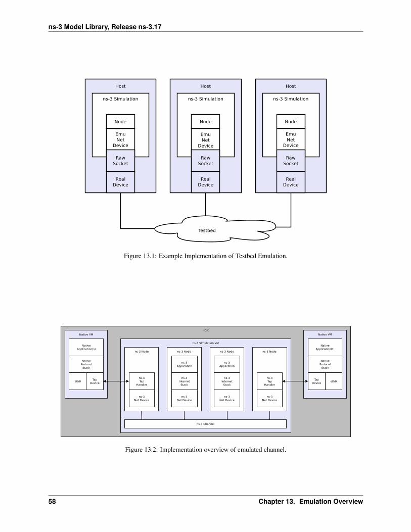
ns-3 Model Library, Release ns-3.17
Figure 13.1: Example Implementation of Testbed Emulation.
Figure 13.2: Implementation overview of emulated channel.
58 Chapter 13. Emulation Overview
ns-3 Model Library, Release ns-3.17
We expect the typical use case for this environment will be to analyze the behavior of native applications and protocolsuites in the presence of large simulated ns-3 networks.
13.1 File Descriptor NetDevice
The src/fd-net-device module provides the FdNetDevice class, which is able to read and write traffic usinga file descriptor provided by the user. This file descriptor can be associated to a TAP device, to a raw socket, to a userspace process generating/consuming traffic, etc. The user has full freedom to define how external traffic is generatedand ns-3 traffic is consumed.
Different mechanisms to associate a simulation to external traffic can be provided through helper classes. Threespecific helpers are provided:
• EmuFdNetDeviceHelper (to associate the ns-3 device with a physical device in the host machine)
• TapFdNetDeviceHelper (to associate the ns-3 device with the file descriptor from a tap device in the host ma-chine)
• PlanteLabFdNetDeviceHelper (to automate the creation of tap devices in PlanetLab nodes, enabling ns-3 simu-lations that can send and receive traffic though the Internet using PlanetLab resource.
13.1.1 Model Description
The source code for this module lives in the directory src/fd-net-device.
The FdNetDevice is a special type of ns-3 NetDevice that reads traffic to and from a file descriptor. That is, unlike puresimulation NetDevice objects that write frames to and from a simulated channel, this FdNetDevice directs frames outof the simulation to a file descriptor. The file descriptor may be associated to a Linux TUN/TAP device, to a socket,or to a user-space process.
It is up to the user of this device to provide a file descriptor. The type of file descriptor being provided determineswhat is being modelled. For instance, if the file descriptor provides a raw socket to a WiFi card on the host machine,the device being modelled is a WiFi device.
From the conceptual “top” of the device looking down, it looks to the simulated node like a device supporting a 48-bitIEEE MAC address that can be bridged, supports broadcast, and uses IPv4 ARP or IPv6 Neighbor Discovery, althoughthese attributes can be tuned on a per-use-case basis.
Design
The FdNetDevice implementation makes use of a reader object, extended from the FdReader class in the ns-3src/core module, which manages a separate thread from the main ns-3 execution thread, in order to read trafficfrom the file descriptor.
Upon invocation of the StartDevice method, the reader object is initialized and starts the reading thread. Beforedevice start, a file descriptor must be previously associated to the FdNetDevice with the SetFileDescriptorinvocation.
The creation and configuration of the file descriptor can be left to a number of helpers, described in more detail below.When this is done, the invocation of SetFileDescriptor is responsibility of the helper and must not be directlyinvoked by the user.
Upon reading an incoming frame from the file descriptor, the reader will pass the frame to the ReceiveCallbackmethod, whose task it is to schedule the reception of the frame by the device as a ns-3 simulation event. Since the newframe is passed from the reader thread to the main ns-3 simulation thread, thread-safety issues are avoided by usingthe ScheduleWithContext call instead of the regular Schedule call.
13.1. File Descriptor NetDevice 59
ns-3 Model Library, Release ns-3.17
In order to avoid overwhelming the scheduler when the incoming data rate is too high, a counter is kept with thenumber of frames that are currently scheduled to be received by the device. If this counter reaches the value given bythe RxQueueSize attribute in the device, then the new frame will be dropped silently.
The actual reception of the new frame by the device occurs when the scheduled FordwarUp method is invoked bythe simulator. This method acts as if a new frame had arrived from a channel attached to the device. The devicethen decapsulates the frame, removing any layer 2 headers, and forwards it to upper network stack layers of the node.The ForwardUp method will remove the frame headers, according to the frame encapsulation type defined by theEncapsulationMode attribute, and invoke the receive callback passing an IP packet.
An extra header, the PI header, can be present when the file descriptor is associated to a TAP device that was createdwithout setting the IFF_NO_PI flag. This extra header is removed if EncapsulationMode is set to DIXPI value.
In the opposite direction, packets generated inside the simulation that are sent out through the device, will be passed tothe Send method, which will in turn invoke the SendFrom method. The latter method will add the necessary layer2 headers, and simply write the newly created frame to the file descriptor.
Scope and Limitations
Users of this device are cautioned that there is no flow control across the file descriptor boundary, when using inemulation mode. That is, in a Linux system, if the speed of writing network packets exceeds the ability of theunderlying physical device to buffer the packets, backpressure up to the writing application will be applied to avoidlocal packet loss. No such flow control is provided across the file descriptor interface, so users must be aware of thislimitation.
As explained before, the RxQueueSize attribute limits the number of packets that can be pending to be received by thedevice. Frames read from the file descriptor while the number of pending packets is in its maximum will be silentlydropped.
The mtu of the device defaults to the Ethernet II MTU value. However, helpers are supposed to set the mtu to the rightvalue to reflect the characteristics of the network interface associated to the file descriptor. If no helper is used, thenthe responsibility of setting the correct mtu value for the device falls back to the user. The size of the read buffer onthe file descriptor reader is set to the mtu value in the StartDevice method.
The FdNetDevice class currently supports three encapsulation modes, DIX for Ethernet II frames, LLC for 802.2LLC/SNAP frames, and DIXPI for Ethernet II frames with an additional TAP PI header. This means that traffictraversing the file descriptor is expected to be Ethernet II compatible. Attaching an FdNetDevice to a wireless interfaceis possible as long as the driver provides Ethernet II frames to the socket API. Note that to associate a FdNetDeviceto a wireless card in ad-hoc mode, the MAC address of the device must be set to the real card MAC address, else anyincoming traffic a fake MAC address will be discarded by the driver.
As mentioned before, three helpers are provided with the fd-net-device module. Each individual helper (file descriptortype) may have platform limitations. For instance, threading, real-time simulation mode, and the ability to createTUN/TAP devices are prerequisites to using the provided helpers. Support for these modes can be found in the outputof the waf configure step, e.g.:
Threading Primitives : enabledReal Time Simulator : enabledEmulated Net Device : enabledTap Bridge : enabled
It is important to mention that while testing the FdNetDevice we have found an upper bound limit for TCP through-put when using 1Gb Ethernet links of 60Mbps. This limit is most likely due to the processing power of the computersinvolved in the tests.
60 Chapter 13. Emulation Overview
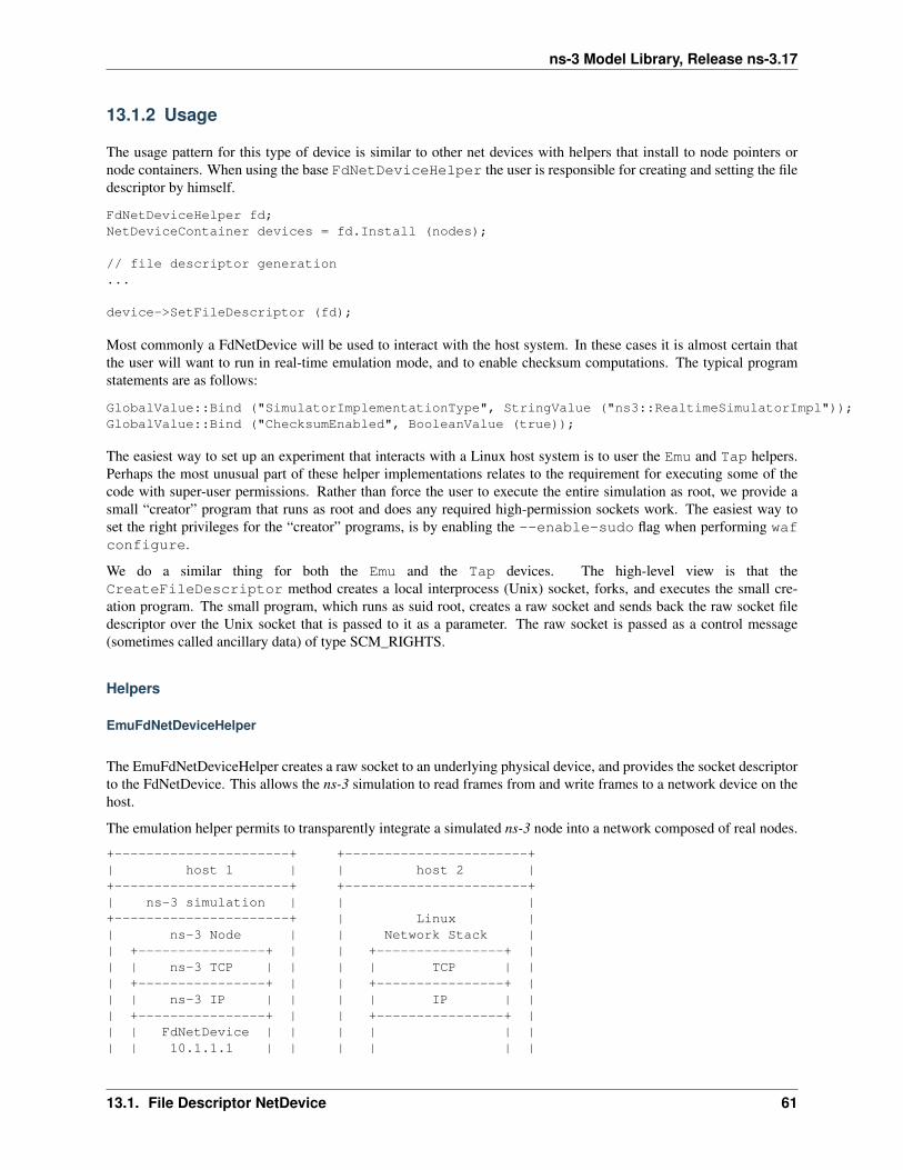
ns-3 Model Library, Release ns-3.17
13.1.2 Usage
The usage pattern for this type of device is similar to other net devices with helpers that install to node pointers ornode containers. When using the base FdNetDeviceHelper the user is responsible for creating and setting the filedescriptor by himself.
FdNetDeviceHelper fd;NetDeviceContainer devices = fd.Install (nodes);
// file descriptor generation...
device->SetFileDescriptor (fd);
Most commonly a FdNetDevice will be used to interact with the host system. In these cases it is almost certain thatthe user will want to run in real-time emulation mode, and to enable checksum computations. The typical programstatements are as follows:
GlobalValue::Bind ("SimulatorImplementationType", StringValue ("ns3::RealtimeSimulatorImpl"));GlobalValue::Bind ("ChecksumEnabled", BooleanValue (true));
The easiest way to set up an experiment that interacts with a Linux host system is to user the Emu and Tap helpers.Perhaps the most unusual part of these helper implementations relates to the requirement for executing some of thecode with super-user permissions. Rather than force the user to execute the entire simulation as root, we provide asmall “creator” program that runs as root and does any required high-permission sockets work. The easiest way toset the right privileges for the “creator” programs, is by enabling the --enable-sudo flag when performing wafconfigure.
We do a similar thing for both the Emu and the Tap devices. The high-level view is that theCreateFileDescriptor method creates a local interprocess (Unix) socket, forks, and executes the small cre-ation program. The small program, which runs as suid root, creates a raw socket and sends back the raw socket filedescriptor over the Unix socket that is passed to it as a parameter. The raw socket is passed as a control message(sometimes called ancillary data) of type SCM_RIGHTS.
Helpers
EmuFdNetDeviceHelper
The EmuFdNetDeviceHelper creates a raw socket to an underlying physical device, and provides the socket descriptorto the FdNetDevice. This allows the ns-3 simulation to read frames from and write frames to a network device on thehost.
The emulation helper permits to transparently integrate a simulated ns-3 node into a network composed of real nodes.
+----------------------+ +-----------------------+| host 1 | | host 2 |+----------------------+ +-----------------------+| ns-3 simulation | | |+----------------------+ | Linux || ns-3 Node | | Network Stack || +----------------+ | | +----------------+ || | ns-3 TCP | | | | TCP | || +----------------+ | | +----------------+ || | ns-3 IP | | | | IP | || +----------------+ | | +----------------+ || | FdNetDevice | | | | | || | 10.1.1.1 | | | | | |
13.1. File Descriptor NetDevice 61
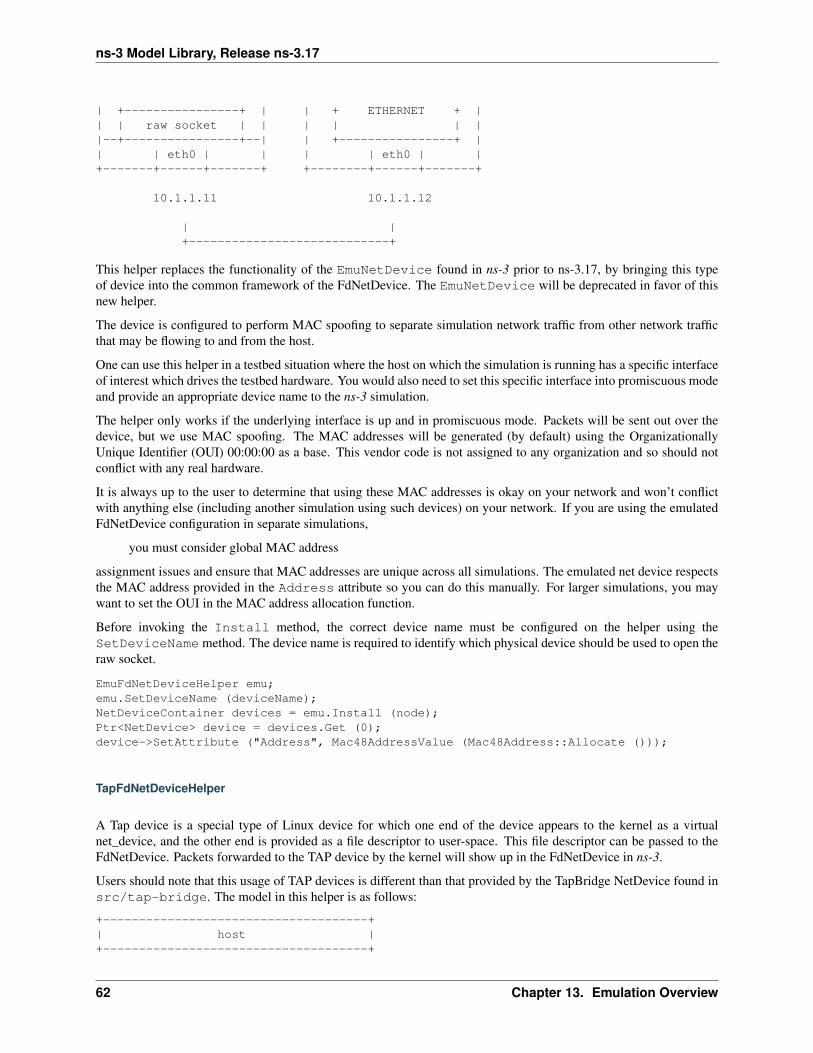
ns-3 Model Library, Release ns-3.17
| +----------------+ | | + ETHERNET + || | raw socket | | | | | ||--+----------------+--| | +----------------+ || | eth0 | | | | eth0 | |+-------+------+-------+ +--------+------+-------+
10.1.1.11 10.1.1.12
| |+----------------------------+
This helper replaces the functionality of the EmuNetDevice found in ns-3 prior to ns-3.17, by bringing this typeof device into the common framework of the FdNetDevice. The EmuNetDevice will be deprecated in favor of thisnew helper.
The device is configured to perform MAC spoofing to separate simulation network traffic from other network trafficthat may be flowing to and from the host.
One can use this helper in a testbed situation where the host on which the simulation is running has a specific interfaceof interest which drives the testbed hardware. You would also need to set this specific interface into promiscuous modeand provide an appropriate device name to the ns-3 simulation.
The helper only works if the underlying interface is up and in promiscuous mode. Packets will be sent out over thedevice, but we use MAC spoofing. The MAC addresses will be generated (by default) using the OrganizationallyUnique Identifier (OUI) 00:00:00 as a base. This vendor code is not assigned to any organization and so should notconflict with any real hardware.
It is always up to the user to determine that using these MAC addresses is okay on your network and won’t conflictwith anything else (including another simulation using such devices) on your network. If you are using the emulatedFdNetDevice configuration in separate simulations,
you must consider global MAC address
assignment issues and ensure that MAC addresses are unique across all simulations. The emulated net device respectsthe MAC address provided in the Address attribute so you can do this manually. For larger simulations, you maywant to set the OUI in the MAC address allocation function.
Before invoking the Install method, the correct device name must be configured on the helper using theSetDeviceName method. The device name is required to identify which physical device should be used to open theraw socket.
EmuFdNetDeviceHelper emu;emu.SetDeviceName (deviceName);NetDeviceContainer devices = emu.Install (node);Ptr<NetDevice> device = devices.Get (0);device->SetAttribute ("Address", Mac48AddressValue (Mac48Address::Allocate ()));
TapFdNetDeviceHelper
A Tap device is a special type of Linux device for which one end of the device appears to the kernel as a virtualnet_device, and the other end is provided as a file descriptor to user-space. This file descriptor can be passed to theFdNetDevice. Packets forwarded to the TAP device by the kernel will show up in the FdNetDevice in ns-3.
Users should note that this usage of TAP devices is different than that provided by the TapBridge NetDevice found insrc/tap-bridge. The model in this helper is as follows:
+-------------------------------------+| host |+-------------------------------------+
62 Chapter 13. Emulation Overview
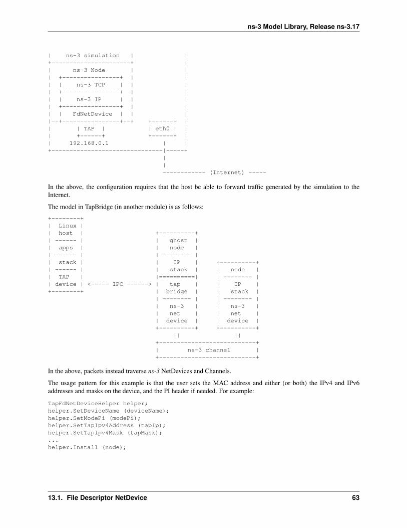
ns-3 Model Library, Release ns-3.17
| ns-3 simulation | |+----------------------+ || ns-3 Node | || +----------------+ | || | ns-3 TCP | | || +----------------+ | || | ns-3 IP | | || +----------------+ | || | FdNetDevice | | ||--+----------------+--+ +------+ || | TAP | | eth0 | || +------+ +------+ || 192.168.0.1 | |+-------------------------------|-----+
||------------ (Internet) -----
In the above, the configuration requires that the host be able to forward traffic generated by the simulation to theInternet.
The model in TapBridge (in another module) is as follows:
+--------+| Linux || host | +----------+| ------ | | ghost || apps | | node || ------ | | -------- || stack | | IP | +----------+| ------ | | stack | | node || TAP | |==========| | -------- || device | <----- IPC ------> | tap | | IP |+--------+ | bridge | | stack |
| -------- | | -------- || ns-3 | | ns-3 || net | | net || device | | device |+----------+ +----------+
|| ||+---------------------------+| ns-3 channel |+---------------------------+
In the above, packets instead traverse ns-3 NetDevices and Channels.
The usage pattern for this example is that the user sets the MAC address and either (or both) the IPv4 and IPv6addresses and masks on the device, and the PI header if needed. For example:
TapFdNetDeviceHelper helper;helper.SetDeviceName (deviceName);helper.SetModePi (modePi);helper.SetTapIpv4Address (tapIp);helper.SetTapIpv4Mask (tapMask);...helper.Install (node);
13.1. File Descriptor NetDevice 63
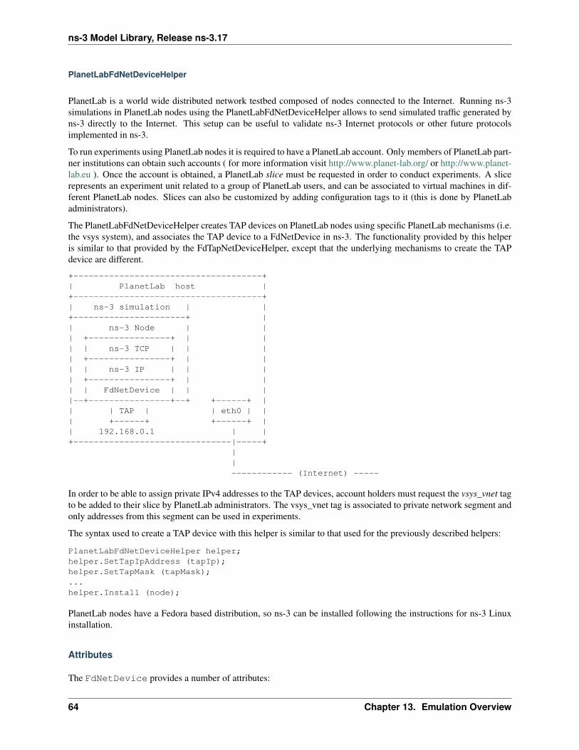
ns-3 Model Library, Release ns-3.17
PlanetLabFdNetDeviceHelper
PlanetLab is a world wide distributed network testbed composed of nodes connected to the Internet. Running ns-3simulations in PlanetLab nodes using the PlanetLabFdNetDeviceHelper allows to send simulated traffic generated byns-3 directly to the Internet. This setup can be useful to validate ns-3 Internet protocols or other future protocolsimplemented in ns-3.
To run experiments using PlanetLab nodes it is required to have a PlanetLab account. Only members of PlanetLab part-ner institutions can obtain such accounts ( for more information visit http://www.planet-lab.org/ or http://www.planet-lab.eu ). Once the account is obtained, a PlanetLab slice must be requested in order to conduct experiments. A slicerepresents an experiment unit related to a group of PlanetLab users, and can be associated to virtual machines in dif-ferent PlanetLab nodes. Slices can also be customized by adding configuration tags to it (this is done by PlanetLabadministrators).
The PlanetLabFdNetDeviceHelper creates TAP devices on PlanetLab nodes using specific PlanetLab mechanisms (i.e.the vsys system), and associates the TAP device to a FdNetDevice in ns-3. The functionality provided by this helperis similar to that provided by the FdTapNetDeviceHelper, except that the underlying mechanisms to create the TAPdevice are different.
+-------------------------------------+| PlanetLab host |+-------------------------------------+| ns-3 simulation | |+----------------------+ || ns-3 Node | || +----------------+ | || | ns-3 TCP | | || +----------------+ | || | ns-3 IP | | || +----------------+ | || | FdNetDevice | | ||--+----------------+--+ +------+ || | TAP | | eth0 | || +------+ +------+ || 192.168.0.1 | |+-------------------------------|-----+
||------------ (Internet) -----
In order to be able to assign private IPv4 addresses to the TAP devices, account holders must request the vsys_vnet tagto be added to their slice by PlanetLab administrators. The vsys_vnet tag is associated to private network segment andonly addresses from this segment can be used in experiments.
The syntax used to create a TAP device with this helper is similar to that used for the previously described helpers:
PlanetLabFdNetDeviceHelper helper;helper.SetTapIpAddress (tapIp);helper.SetTapMask (tapMask);...helper.Install (node);
PlanetLab nodes have a Fedora based distribution, so ns-3 can be installed following the instructions for ns-3 Linuxinstallation.
Attributes
The FdNetDevice provides a number of attributes:
64 Chapter 13. Emulation Overview
ns-3 Model Library, Release ns-3.17
• Address: The MAC address of the device
• Start: The simulation start time to spin up the device thread
• Stop: The simulation start time to stop the device thread
• EncapsulationMode: Link-layer encapsulation format
• RxQueueSize: The buffer size of the read queue on the file descriptor thread (default of 1000 packets)
Start and Stop do not normally need to be specified unless the user wants to limit the time during which this deviceis active. Address needs to be set to some kind of unique MAC address if the simulation will be interacting withother real devices somehow using real MAC addresses. Typical code:
device->SetAttribute ("Address", Mac48AddressValue (Mac48Address::Allocate ()));
Output
Ascii and PCAP tracing is provided similar to the other ns-3 NetDevice types, through the helpers, such as (e.g.):
:: EmuFdNetDeviceHelper emu; NetDeviceContainer devices = emu.Install (node); ... emu.EnablePcap (“emu-ping”,device, true);
The standard set of Mac-level NetDevice trace sources is provided.
• MaxTx: Trace source triggered when ns-3 provides the device with a new frame to send
• MaxTxDrop: Trace source if write to file descriptor fails
• MaxPromiscRx: Whenever any valid Mac frame is received
• MaxRx: Whenever a valid Mac frame is received for this device
• Sniffer: Non-promiscuous packet sniffer
• PromiscSniffer: Promiscuous packet sniffer (for tcpdump-like traces)
Examples
Several examples are provided:
• dummy-network.cc: This simple example creates two nodes and interconnects them with a Unix pipe bypassing the file descriptors from the socketpair into the FdNetDevice objects of the respective nodes.
• realtime-dummy-network.cc: Same as dummy-network.cc but uses the real time simulator implement-nation instead of the default one.
• fd2fd-onoff.cc: This example is aimed at measuring the throughput of the FdNetDevice in a pure simu-lation. For this purpose two FdNetDevices, attached to different nodes but in a same simulation, are connectedusing a socket pair. TCP traffic is sent at a saturating data rate.
• fd-emu-onoff.cc: This example is aimed at measuring the throughput of the FdNetDevice when using theEmuFdNetDeviceHelper to attach the simulated device to a real device in the host machine. This is achieved bysaturating the channel with TCP traffic.
• fd-emu-ping.cc: This example uses the EmuFdNetDeviceHelper to send ICMP traffic over a real channel.
• fd-emu-udp-echo.cc: This example uses the EmuFdNetDeviceHelper to send UDP traffic over a realchannel.
• fd-planetlab-ping.cc: This example shows how to set up an experiment to send ICMP traffic from aPlanetLab node to the Internet.
13.1. File Descriptor NetDevice 65
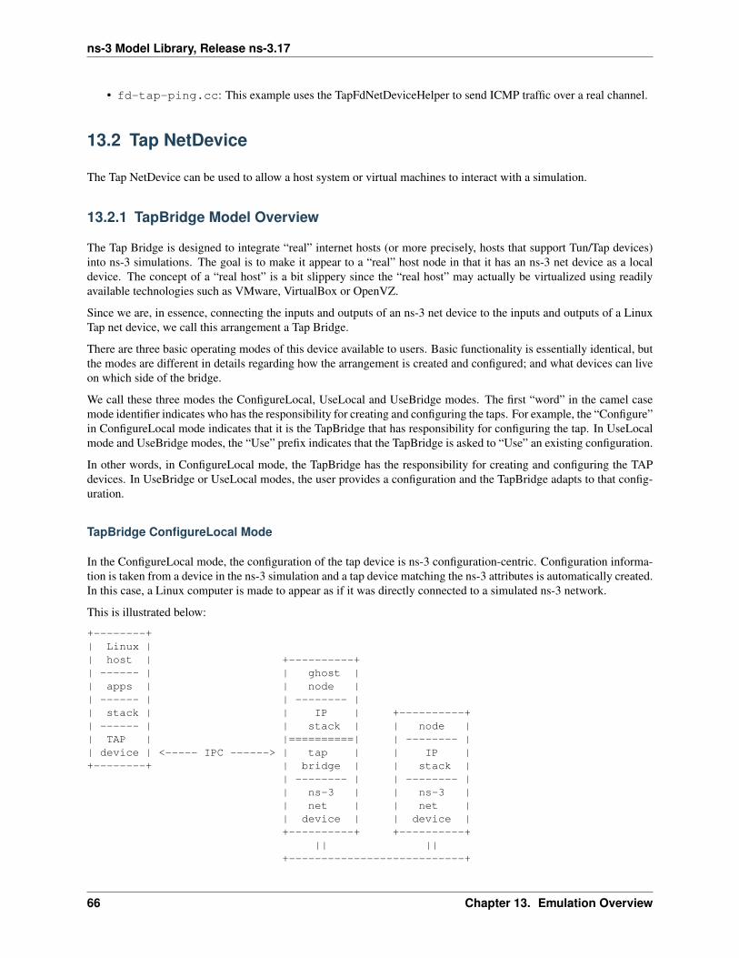
ns-3 Model Library, Release ns-3.17
• fd-tap-ping.cc: This example uses the TapFdNetDeviceHelper to send ICMP traffic over a real channel.
13.2 Tap NetDevice
The Tap NetDevice can be used to allow a host system or virtual machines to interact with a simulation.
13.2.1 TapBridge Model Overview
The Tap Bridge is designed to integrate “real” internet hosts (or more precisely, hosts that support Tun/Tap devices)into ns-3 simulations. The goal is to make it appear to a “real” host node in that it has an ns-3 net device as a localdevice. The concept of a “real host” is a bit slippery since the “real host” may actually be virtualized using readilyavailable technologies such as VMware, VirtualBox or OpenVZ.
Since we are, in essence, connecting the inputs and outputs of an ns-3 net device to the inputs and outputs of a LinuxTap net device, we call this arrangement a Tap Bridge.
There are three basic operating modes of this device available to users. Basic functionality is essentially identical, butthe modes are different in details regarding how the arrangement is created and configured; and what devices can liveon which side of the bridge.
We call these three modes the ConfigureLocal, UseLocal and UseBridge modes. The first “word” in the camel casemode identifier indicates who has the responsibility for creating and configuring the taps. For example, the “Configure”in ConfigureLocal mode indicates that it is the TapBridge that has responsibility for configuring the tap. In UseLocalmode and UseBridge modes, the “Use” prefix indicates that the TapBridge is asked to “Use” an existing configuration.
In other words, in ConfigureLocal mode, the TapBridge has the responsibility for creating and configuring the TAPdevices. In UseBridge or UseLocal modes, the user provides a configuration and the TapBridge adapts to that config-uration.
TapBridge ConfigureLocal Mode
In the ConfigureLocal mode, the configuration of the tap device is ns-3 configuration-centric. Configuration informa-tion is taken from a device in the ns-3 simulation and a tap device matching the ns-3 attributes is automatically created.In this case, a Linux computer is made to appear as if it was directly connected to a simulated ns-3 network.
This is illustrated below:
+--------+| Linux || host | +----------+| ------ | | ghost || apps | | node || ------ | | -------- || stack | | IP | +----------+| ------ | | stack | | node || TAP | |==========| | -------- || device | <----- IPC ------> | tap | | IP |+--------+ | bridge | | stack |
| -------- | | -------- || ns-3 | | ns-3 || net | | net || device | | device |+----------+ +----------+
|| ||+---------------------------+
66 Chapter 13. Emulation Overview
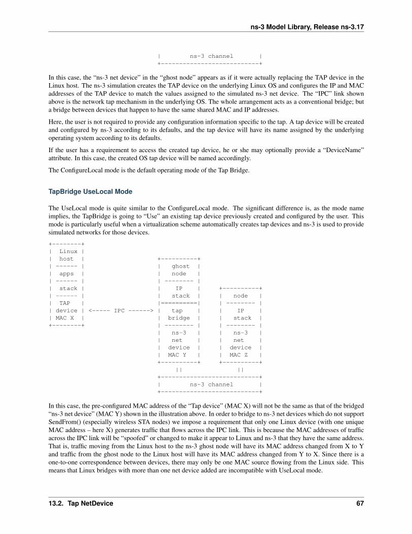
ns-3 Model Library, Release ns-3.17
| ns-3 channel |+---------------------------+
In this case, the “ns-3 net device” in the “ghost node” appears as if it were actually replacing the TAP device in theLinux host. The ns-3 simulation creates the TAP device on the underlying Linux OS and configures the IP and MACaddresses of the TAP device to match the values assigned to the simulated ns-3 net device. The “IPC” link shownabove is the network tap mechanism in the underlying OS. The whole arrangement acts as a conventional bridge; buta bridge between devices that happen to have the same shared MAC and IP addresses.
Here, the user is not required to provide any configuration information specific to the tap. A tap device will be createdand configured by ns-3 according to its defaults, and the tap device will have its name assigned by the underlyingoperating system according to its defaults.
If the user has a requirement to access the created tap device, he or she may optionally provide a “DeviceName”attribute. In this case, the created OS tap device will be named accordingly.
The ConfigureLocal mode is the default operating mode of the Tap Bridge.
TapBridge UseLocal Mode
The UseLocal mode is quite similar to the ConfigureLocal mode. The significant difference is, as the mode nameimplies, the TapBridge is going to “Use” an existing tap device previously created and configured by the user. Thismode is particularly useful when a virtualization scheme automatically creates tap devices and ns-3 is used to providesimulated networks for those devices.
+--------+| Linux || host | +----------+| ------ | | ghost || apps | | node || ------ | | -------- || stack | | IP | +----------+| ------ | | stack | | node || TAP | |==========| | -------- || device | <----- IPC ------> | tap | | IP || MAC X | | bridge | | stack |+--------+ | -------- | | -------- |
| ns-3 | | ns-3 || net | | net || device | | device || MAC Y | | MAC Z |+----------+ +----------+
|| ||+---------------------------+| ns-3 channel |+---------------------------+
In this case, the pre-configured MAC address of the “Tap device” (MAC X) will not be the same as that of the bridged“ns-3 net device” (MAC Y) shown in the illustration above. In order to bridge to ns-3 net devices which do not supportSendFrom() (especially wireless STA nodes) we impose a requirement that only one Linux device (with one uniqueMAC address – here X) generates traffic that flows across the IPC link. This is because the MAC addresses of trafficacross the IPC link will be “spoofed” or changed to make it appear to Linux and ns-3 that they have the same address.That is, traffic moving from the Linux host to the ns-3 ghost node will have its MAC address changed from X to Yand traffic from the ghost node to the Linux host will have its MAC address changed from Y to X. Since there is aone-to-one correspondence between devices, there may only be one MAC source flowing from the Linux side. Thismeans that Linux bridges with more than one net device added are incompatible with UseLocal mode.
13.2. Tap NetDevice 67
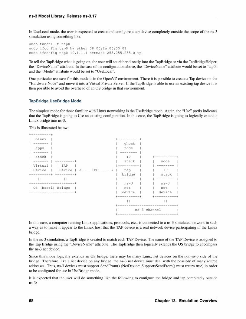
ns-3 Model Library, Release ns-3.17
In UseLocal mode, the user is expected to create and configure a tap device completely outside the scope of the ns-3simulation using something like:
sudo tunctl -t tap0sudo ifconfig tap0 hw ether 08:00:2e:00:00:01sudo ifconfig tap0 10.1.1.1 netmask 255.255.255.0 up
To tell the TapBridge what is going on, the user will set either directly into the TapBridge or via the TapBridgeHelper,the “DeviceName” attribute. In the case of the configuration above, the “DeviceName” attribute would be set to “tap0”and the “Mode” attribute would be set to “UseLocal”.
One particular use case for this mode is in the OpenVZ environment. There it is possible to create a Tap device on the“Hardware Node” and move it into a Virtual Private Server. If the TapBridge is able to use an existing tap device it isthen possible to avoid the overhead of an OS bridge in that environment.
TapBridge UseBridge Mode
The simplest mode for those familiar with Linux networking is the UseBridge mode. Again, the “Use” prefix indicatesthat the TapBridge is going to Use an existing configuration. In this case, the TapBridge is going to logically extend aLinux bridge into ns-3.
This is illustrated below:
+---------+| Linux | +----------+| ------- | | ghost || apps | | node || ------- | | -------- || stack | | IP | +----------+| ------- | +--------+ | stack | | node || Virtual | | TAP | |==========| | -------- || Device | | Device | <---- IPC -----> | tap | | IP |+---------+ +--------+ | bridge | | stack |
|| || | -------- | | -------- |+--------------------+ | ns-3 | | ns-3 || OS (brctl) Bridge | | net | | net |+--------------------+ | device | | device |
+----------+ +----------+|| ||
+---------------------------+| ns-3 channel |+---------------------------+
In this case, a computer running Linux applications, protocols, etc., is connected to a ns-3 simulated network in sucha way as to make it appear to the Linux host that the TAP device is a real network device participating in the Linuxbridge.
In the ns-3 simulation, a TapBridge is created to match each TAP Device. The name of the TAP Device is assigned tothe Tap Bridge using the “DeviceName” attribute. The TapBridge then logically extends the OS bridge to encompassthe ns-3 net device.
Since this mode logically extends an OS bridge, there may be many Linux net devices on the non-ns-3 side of thebridge. Therefore, like a net device on any bridge, the ns-3 net device must deal with the possibly of many sourceaddresses. Thus, ns-3 devices must support SendFrom() (NetDevice::SupportsSendFrom() must return true) in orderto be configured for use in UseBridge mode.
It is expected that the user will do something like the following to configure the bridge and tap completely outsidens-3:
68 Chapter 13. Emulation Overview
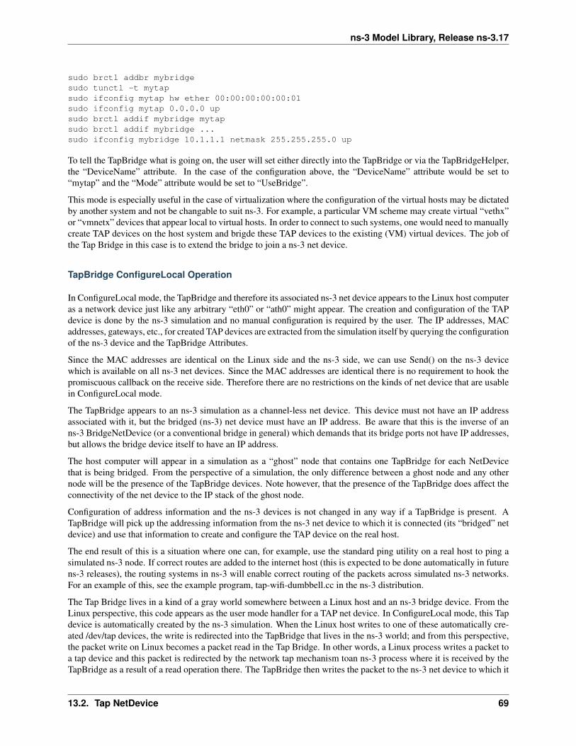
ns-3 Model Library, Release ns-3.17
sudo brctl addbr mybridgesudo tunctl -t mytapsudo ifconfig mytap hw ether 00:00:00:00:00:01sudo ifconfig mytap 0.0.0.0 upsudo brctl addif mybridge mytapsudo brctl addif mybridge ...sudo ifconfig mybridge 10.1.1.1 netmask 255.255.255.0 up
To tell the TapBridge what is going on, the user will set either directly into the TapBridge or via the TapBridgeHelper,the “DeviceName” attribute. In the case of the configuration above, the “DeviceName” attribute would be set to“mytap” and the “Mode” attribute would be set to “UseBridge”.
This mode is especially useful in the case of virtualization where the configuration of the virtual hosts may be dictatedby another system and not be changable to suit ns-3. For example, a particular VM scheme may create virtual “vethx”or “vmnetx” devices that appear local to virtual hosts. In order to connect to such systems, one would need to manuallycreate TAP devices on the host system and brigde these TAP devices to the existing (VM) virtual devices. The job ofthe Tap Bridge in this case is to extend the bridge to join a ns-3 net device.
TapBridge ConfigureLocal Operation
In ConfigureLocal mode, the TapBridge and therefore its associated ns-3 net device appears to the Linux host computeras a network device just like any arbitrary “eth0” or “ath0” might appear. The creation and configuration of the TAPdevice is done by the ns-3 simulation and no manual configuration is required by the user. The IP addresses, MACaddresses, gateways, etc., for created TAP devices are extracted from the simulation itself by querying the configurationof the ns-3 device and the TapBridge Attributes.
Since the MAC addresses are identical on the Linux side and the ns-3 side, we can use Send() on the ns-3 devicewhich is available on all ns-3 net devices. Since the MAC addresses are identical there is no requirement to hook thepromiscuous callback on the receive side. Therefore there are no restrictions on the kinds of net device that are usablein ConfigureLocal mode.
The TapBridge appears to an ns-3 simulation as a channel-less net device. This device must not have an IP addressassociated with it, but the bridged (ns-3) net device must have an IP address. Be aware that this is the inverse of anns-3 BridgeNetDevice (or a conventional bridge in general) which demands that its bridge ports not have IP addresses,but allows the bridge device itself to have an IP address.
The host computer will appear in a simulation as a “ghost” node that contains one TapBridge for each NetDevicethat is being bridged. From the perspective of a simulation, the only difference between a ghost node and any othernode will be the presence of the TapBridge devices. Note however, that the presence of the TapBridge does affect theconnectivity of the net device to the IP stack of the ghost node.
Configuration of address information and the ns-3 devices is not changed in any way if a TapBridge is present. ATapBridge will pick up the addressing information from the ns-3 net device to which it is connected (its “bridged” netdevice) and use that information to create and configure the TAP device on the real host.
The end result of this is a situation where one can, for example, use the standard ping utility on a real host to ping asimulated ns-3 node. If correct routes are added to the internet host (this is expected to be done automatically in futurens-3 releases), the routing systems in ns-3 will enable correct routing of the packets across simulated ns-3 networks.For an example of this, see the example program, tap-wifi-dumbbell.cc in the ns-3 distribution.
The Tap Bridge lives in a kind of a gray world somewhere between a Linux host and an ns-3 bridge device. From theLinux perspective, this code appears as the user mode handler for a TAP net device. In ConfigureLocal mode, this Tapdevice is automatically created by the ns-3 simulation. When the Linux host writes to one of these automatically cre-ated /dev/tap devices, the write is redirected into the TapBridge that lives in the ns-3 world; and from this perspective,the packet write on Linux becomes a packet read in the Tap Bridge. In other words, a Linux process writes a packet toa tap device and this packet is redirected by the network tap mechanism toan ns-3 process where it is received by theTapBridge as a result of a read operation there. The TapBridge then writes the packet to the ns-3 net device to which it
13.2. Tap NetDevice 69
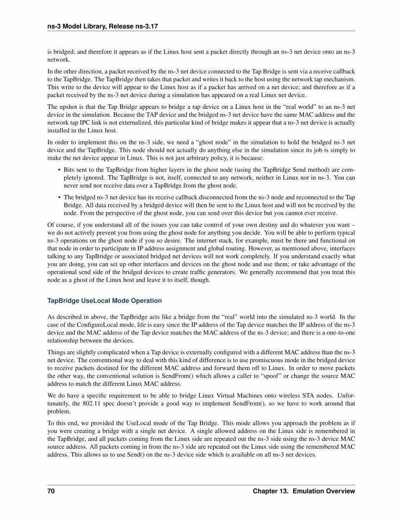
ns-3 Model Library, Release ns-3.17
is bridged; and therefore it appears as if the Linux host sent a packet directly through an ns-3 net device onto an ns-3network.
In the other direction, a packet received by the ns-3 net device connected to the Tap Bridge is sent via a receive callbackto the TapBridge. The TapBridge then takes that packet and writes it back to the host using the network tap mechanism.This write to the device will appear to the Linux host as if a packet has arrived on a net device; and therefore as if apacket received by the ns-3 net device during a simulation has appeared on a real Linux net device.
The upshot is that the Tap Bridge appears to bridge a tap device on a Linux host in the “real world” to an ns-3 netdevice in the simulation. Because the TAP device and the bridged ns-3 net device have the same MAC address and thenetwork tap IPC link is not externalized, this particular kind of bridge makes it appear that a ns-3 net device is actuallyinstalled in the Linux host.
In order to implement this on the ns-3 side, we need a “ghost node” in the simulation to hold the bridged ns-3 netdevice and the TapBridge. This node should not actually do anything else in the simulation since its job is simply tomake the net device appear in Linux. This is not just arbitrary policy, it is because:
• Bits sent to the TapBridge from higher layers in the ghost node (using the TapBridge Send method) are com-pletely ignored. The TapBridge is not, itself, connected to any network, neither in Linux nor in ns-3. You cannever send nor receive data over a TapBridge from the ghost node.
• The bridged ns-3 net device has its receive callback disconnected from the ns-3 node and reconnected to the TapBridge. All data received by a bridged device will then be sent to the Linux host and will not be received by thenode. From the perspective of the ghost node, you can send over this device but you cannot ever receive.
Of course, if you understand all of the issues you can take control of your own destiny and do whatever you want –we do not actively prevent you from using the ghost node for anything you decide. You will be able to perform typicalns-3 operations on the ghost node if you so desire. The internet stack, for example, must be there and functional onthat node in order to participate in IP address assignment and global routing. However, as mentioned above, interfacestalking to any TapBridge or associated bridged net devices will not work completely. If you understand exactly whatyou are doing, you can set up other interfaces and devices on the ghost node and use them; or take advantage of theoperational send side of the bridged devices to create traffic generators. We generally recommend that you treat thisnode as a ghost of the Linux host and leave it to itself, though.
TapBridge UseLocal Mode Operation
As described in above, the TapBridge acts like a bridge from the “real” world into the simulated ns-3 world. In thecase of the ConfigureLocal mode, life is easy since the IP address of the Tap device matches the IP address of the ns-3device and the MAC address of the Tap device matches the MAC address of the ns-3 device; and there is a one-to-onerelationship between the devices.
Things are slightly complicated when a Tap device is externally configured with a different MAC address than the ns-3net device. The conventional way to deal with this kind of difference is to use promiscuous mode in the bridged deviceto receive packets destined for the different MAC address and forward them off to Linux. In order to move packetsthe other way, the conventional solution is SendFrom() which allows a caller to “spoof” or change the source MACaddress to match the different Linux MAC address.
We do have a specific requirement to be able to bridge Linux Virtual Machines onto wireless STA nodes. Unfor-tunately, the 802.11 spec doesn’t provide a good way to implement SendFrom(), so we have to work around thatproblem.
To this end, we provided the UseLocal mode of the Tap Bridge. This mode allows you approach the problem as ifyou were creating a bridge with a single net device. A single allowed address on the Linux side is remembered inthe TapBridge, and all packets coming from the Linux side are repeated out the ns-3 side using the ns-3 device MACsource address. All packets coming in from the ns-3 side are repeated out the Linux side using the remembered MACaddress. This allows us to use Send() on the ns-3 device side which is available on all ns-3 net devices.
70 Chapter 13. Emulation Overview

ns-3 Model Library, Release ns-3.17
UseLocal mode is identical to the ConfigureLocal mode except for the creation and configuration of the tap device andthe MAC address spoofing.
TapBridge UseBridge Operation
As described in the ConfigureLocal mode section, when the Linux host writes to one of the /dev/tap devices, the writeis redirected into the TapBridge that lives in the ns-3 world. In the case of the UseBridge mode, these packets willneed to be sent out on the ns-3 network as if they were sent on a device participating in the Linux bridge. This meanscalling the SendFrom() method on the bridged device and providing the source MAC address found in the packet.
In the other direction, a packet received by an ns-3 net device is hooked via callback to the TapBridge. This must bedone in promiscuous mode since the goal is to bridge the ns-3 net device onto the OS (brctl) bridge of which the TAPdevice is a part.
For these reasons, only ns-3 net devices that support SendFrom() and have a hookable promiscuous receive callbackare allowed to participate in UseBridge mode TapBridge configurations.
13.2.2 Tap Bridge Channel Model
There is no channel model associated with the Tap Bridge. In fact, the intention is make it appear that the real internethost is connected to the channel of the bridged net device.
13.2.3 Tap Bridge Tracing Model
Unlike most ns-3 devices, the TapBridge does not provide any standard trace sources. This is because the bridge is anintermediary that is essentially one function call away from the bridged device. We expect that the trace hooks in thebridged device will be sufficient for most users,
13.2.4 Using the TapBridge
We expect that most users will interact with the TapBridge device through the TapBridgeHelper. Users of other helperclasses, such as CSMA or Wifi, should be comfortable with the idioms used there.
13.2. Tap NetDevice 71

ns-3 Model Library, Release ns-3.17
72 Chapter 13. Emulation Overview
CHAPTER
FOURTEEN
ENERGY FRAMEWORK
Energy consumption is a key issue for wireless devices, and wireless network researchers often need to investigate theenergy consumption at a node or in the overall network while running network simulations in ns-3. This requires ns-3to support energy consumption modeling. Further, as concepts such as fuel cells and energy scavenging are becomingviable for low power wireless devices, incorporating the effect of these emerging technologies into simulations requiressupport for modeling diverse energy sources in ns-3. The ns-3 Energy Framework provides the basis for energyconsumption and energy source modeling.
14.1 Model Description
The source code for the Energy Framework is currently at: src/energy.
14.1.1 Design
The ns-3 Energy Framework is composed of 2 parts: Energy Source and Device Energy Model. The framework willbe implemented into the src/energy/models folder.
Energy Source
The Energy Source represents the power supply on each node. A node can have one or more energy sources, andeach energy source can be connected to multiple device energy models. Connecting an energy source to a deviceenergy model implies that the corresponding device draws power from the source. The basic functionality of theEnergy Source is to provide energy for devices on the node. When energy is completely drained from the EnergySource, it notifies the devices on node such that each device can react to this event. Further, each node can access theEnergy Source Objects for information such as remaining energy or energy fraction (battery level). This enables theimplementation of energy aware protocols in ns-3.
In order to model a wide range of power supplies such as batteries, the Energy Source must be able to capture charac-teristics of these supplies. There are 2 important characteristics or effects related to practical batteries:
• Rate Capacity Effect: Decrease of battery lifetime when the current draw is higher than the rated value of thebattery.
• Recovery Effect: Increase of battery lifetime when the battery is alternating between discharge and idle states.
In order to incorporate the Rate Capacity Effect, the Energy Source uses current draw from all devices on the samenode to calculate energy consumption. The Energy Source polls all devices on the same node periodically to calculatethe total current draw and hence the energy consumption. When a device changes state, its corresponding DeviceEnergy Model will notify the Energy Source of this change and new total current draw will be calculated.
73

ns-3 Model Library, Release ns-3.17
The Energy Source base class keeps a list of devices (Device Energy Model objects) using the particular EnergySource as power supply. When energy is completely drained, the Energy Source will notify all devices on this list.Each device can then handle this event independently, based on the desired behavior when power supply is drained.
Device Energy Model
The Device Energy Model is the energy consumption model of a device on node. It is designed to be a state basedmodel where each device is assumed to have a number of states, and each state is associated with a power consumptionvalue. Whenever the state of the device changes, the corresponding Device Energy Model will notify the EnergySource of the new current draw of the device. The Energy Source will then calculate the new total current draw andupdate the remaining energy.
The Device Energy Model can also be used for devices that do not have finite number of states. For example, in anelectric vehicle, the current draw of the motor is determined by its speed. Since the vehicle’s speed can take continuousvalues within a certain range, it is infeasible to define a set of discrete states of operation. However, by converting thespeed value into current directly, the same set of Device Energy Model APIs can still be used.
14.1.2 Future Work
For Device Energy Models, we are planning to include support for other PHY layer models provided in ns-3 such asWiMAX. For Energy Sources, we are planning to included new types of Energy Sources such as energy scavenging.
14.1.3 References
14.2 Usage
The main way that ns-3 users will typically interact with the Energy Framework is through the helper API and throughthe publicly visible attributes of the framework. The helper API is defined in src/energy/helper/*.h.
In order to use the energy framework, the user must install an Energy Source for the node of interest and the cor-responding Device Energy Model for the network devices. Energy Source (objects) are aggregated onto each nodeby the Energy Source Helper. In order to allow multiple energy sources per node, we aggregate an Energy SourceContainer rather than directly aggregating a source object.
The Energy Source object also keeps a list of Device Energy Model objects using the source as power supply. DeviceEnergy Model objects are installed onto the Energy Source by the Device Energy Model Helper. User can accessthe Device Energy Model objects through the Energy Source object to obtain energy consumption information ofindividual devices.
14.2.1 Examples
The example directories, src/examples/energy and examples/energy, contain some basic code that showshow to set up the framework.
14.2.2 Helpers
Energy Source Helper
Base helper class for Energy Source objects, this helper Aggregates Energy Source object onto a node. Child imple-mentation of this class creates the actual Energy Source object.
74 Chapter 14. Energy Framework

ns-3 Model Library, Release ns-3.17
Device Energy Model Helper
Base helper class for Device Energy Model objects, this helper attaches Device Energy Model objects onto EnergySource objects. Child implementation of this class creates the actual Device Energy Model object.
14.2.3 Attributes
Attributes differ between Energy Sources and Devices Energy Models implementations, please look at the specificchild class for details.
Basic Energy Source
• BasicEnergySourceInitialEnergyJ: Initial energy stored in basic energy source.
• BasicEnergySupplyVoltageV: Initial supply voltage for basic energy source.
• PeriodicEnergyUpdateInterval: Time between two consecutive periodic energy updates.
RV Battery Model
• RvBatteryModelPeriodicEnergyUpdateInterval: RV battery model sampling interval.
• RvBatteryModelOpenCircuitVoltage: RV battery model open circuit voltage.
• RvBatteryModelCutoffVoltage: RV battery model cutoff voltage.
• RvBatteryModelAlphaValue: RV battery model alpha value.
• RvBatteryModelBetaValue: RV battery model beta value.
• RvBatteryModelNumOfTerms: The number of terms of the infinite sum for estimating battery level.
WiFi Radio Energy Model
• IdleCurrentA: The default radio Idle current in Ampere.
• CcaBusyCurrentA: The default radio CCA Busy State current in Ampere.
• TxCurrentA: The radio Tx current in Ampere.
• RxCurrentA: The radio Rx current in Ampere.
• SwitchingCurrentA: The default radio Channel Switch current in Ampere.
14.2.4 Tracing
Traced values differ between Energy Sources and Devices Energy Models implementations, please look at the specificchild class for details.
Basic Energy Source
• RemainingEnergy: Remaining energy at BasicEnergySource.
14.2. Usage 75

ns-3 Model Library, Release ns-3.17
RV Battery Model
• RvBatteryModelBatteryLevel: RV battery model battery level.
• RvBatteryModelBatteryLifetime: RV battery model battery lifetime.
WiFi Radio Energy Model
• TotalEnergyConsumption: Total energy consumption of the radio device.
14.2.5 Validation
Comparison of the Energy Framework against actual devices have not been performed. Current implementation of theEnergy Framework is checked numerically for computation errors. The RV battery model is validated by comparingresults with what was presented in the original RV battery model paper.
76 Chapter 14. Energy Framework

CHAPTER
FIFTEEN
FLOW MONITOR
Placeholder chapter
This feature was added as contributed code (src/contrib) in ns-3.6 and to the main distribution(src/flow-monitor) for ns-3.7. A paper on this feature is published in the proceedings of NSTools:http://www.nstools.org/techprog.shtml.
77

ns-3 Model Library, Release ns-3.17
78 Chapter 15. Flow Monitor
CHAPTER
SIXTEEN
INTERNET MODELS
16.1 Internet Stack
16.1.1 Internet stack aggregation
A bare class Node is not very useful as-is; other objects must be aggregated to it to provide useful node functionality.
The ns-3 source code directory src/internet provides implementation of TCP/IPv4- and IPv6-related compo-nents. These include IPv4, ARP, UDP, TCP, IPv6, Neighbor Discovery, and other related protocols.
Internet Nodes are not subclasses of class Node; they are simply Nodes that have had a bunch ofIPv4-related objects aggregated to them. They can be put together by hand, or via a helper functionInternetStackHelper::Install () which does the following to all nodes passed in as arguments::
voidInternetStackHelper::Install (Ptr<Node> node) const{
if (node->GetObject<Ipv4> () != 0){
NS_FATAL_ERROR ("InternetStackHelper::Install(): Aggregating ""an InternetStack to a node with an existing Ipv4 object");
return;}
CreateAndAggregateObjectFromTypeId (node, "ns3::ArpL3Protocol");CreateAndAggregateObjectFromTypeId (node, "ns3::Ipv4L3Protocol");CreateAndAggregateObjectFromTypeId (node, "ns3::Icmpv4L4Protocol");CreateAndAggregateObjectFromTypeId (node, "ns3::UdpL4Protocol");node->AggregateObject (m_tcpFactory.Create<Object> ());Ptr<PacketSocketFactory> factory = CreateObject<PacketSocketFactory> ();node->AggregateObject (factory);// Set routingPtr<Ipv4> ipv4 = node->GetObject<Ipv4> ();Ptr<Ipv4RoutingProtocol> ipv4Routing = m_routing->Create (node);ipv4->SetRoutingProtocol (ipv4Routing);
}
Where multiple implementations exist in ns-3 (TCP, IP routing), these objects are added by a factory object (TCP) orby a routing helper (m_routing).
Note that the routing protocol is configured and set outside this function. By default, the following protocols are addedto Ipv4::
79
ns-3 Model Library, Release ns-3.17
InternetStackHelper::InternetStackHelper (){
SetTcp ("ns3::TcpL4Protocol");static Ipv4StaticRoutingHelper staticRouting;static Ipv4GlobalRoutingHelper globalRouting;static Ipv4ListRoutingHelper listRouting;listRouting.Add (staticRouting, 0);listRouting.Add (globalRouting, -10);SetRoutingHelper (listRouting);
}
By default, IPv4 and IPv6 are enabled.
Internet Node structure
An IPv4-capable Node (an ns-3 Node augmented by aggregation to have one or more IP stacks) has the followinginternal structure.
Layer-3 protocols
At the lowest layer, sitting above the NetDevices, are the “layer 3” protocols, including IPv4, IPv6, and ARP.The class Ipv4L3Protocol is an implementation class whose public interface is typically class Ipv4, but theIpv4L3Protocol public API is also used internally at present.
In class Ipv4L3Protocol, one method described below is Receive ()::
/*** Lower layer calls this method after calling L3Demux::Lookup
* The ARP subclass needs to know from which NetDevice this
* packet is coming to:
* - implement a per-NetDevice ARP cache
* - send back arp replies on the right device
*/void Receive( Ptr<NetDevice> device, Ptr<const Packet> p, uint16_t protocol,
const Address &from, const Address &to, NetDevice::PacketType packetType);
First, note that the Receive () function has a matching signature to the ReceiveCallback in the class Node. Thisfunction pointer is inserted into the Node’s protocol handler when AddInterface () is called. The actual regis-tration is done with a statement such as follows::
RegisterProtocolHandler ( MakeCallback (&Ipv4Protocol::Receive, ipv4),Ipv4L3Protocol::PROT_NUMBER, 0);
The Ipv4L3Protocol object is aggregated to the Node; there is only one such Ipv4L3Protocol object. Higher-layerprotocols that have a packet to send down to the Ipv4L3Protocol object can call GetObject<Ipv4L3Protocol>() to obtain a pointer, as follows::
Ptr<Ipv4L3Protocol> ipv4 = m_node->GetObject<Ipv4L3Protocol> ();if (ipv4 != 0)
{ipv4->Send (packet, saddr, daddr, PROT_NUMBER);
}
This class nicely demonstrates two techniques we exploit in ns-3 to bind objects together: callbacks, and objectaggregation.
80 Chapter 16. Internet Models
ns-3 Model Library, Release ns-3.17
Once IPv4 routing has determined that a packet is for the local node, it forwards it up the stack. This is done with thefollowing function::
voidIpv4L3Protocol::LocalDeliver (Ptr<const Packet> packet, Ipv4Header const&ip, uint32_t iif)
The first step is to find the right Ipv4L4Protocol object, based on IP protocol number. For instance, TCP is reg-istered in the demux as protocol number 6. Finally, the Receive() function on the Ipv4L4Protocol (such asTcpL4Protocol::Receive is called.
We have not yet introduced the class Ipv4Interface. Basically, each NetDevice is paired with an IPv4 representationof such device. In Linux, this class Ipv4Interface roughly corresponds to the struct in_device; the mainpurpose is to provide address-family specific information (addresses) about an interface.
All the classes have appropriate traces in order to track sent, received and lost packets. The users is encouraged touse them so to find out if (and where) a packet is dropped. A common mistake is to forget the effects of local queueswhen sending packets, e.g., the ARP queue. This can be particularly puzzling when sending jumbo packets or packetbursts using UDP. The ARP cache pending queue is limited (3 datagrams) and IP packets might be fragmented, easilyoverfilling the ARP cache queue size. In those cases it is useful to increase the ARP cache pending size to a propervalue, e.g.::
Config::SetDefault ("ns3::ArpCache::PendingQueueSize", UintegerValue (MAX_BURST_SIZE/L2MTU*3));
The IPv6 implementation follows a similar architecture. Dual-stacked nodes (one with support for both IPv4 and IPv6)will allow an IPv6 socket to receive IPv4 connections as a standard dual-stacked system does. A socket bound andlistening to an IPv6 endpoint can receive an IPv4 connection and will return the remote address as an IPv4-mappedaddress. Support for the IPV6_V6ONLY socket option does not currently exist.
Layer-4 protocols and sockets
We next describe how the transport protocols, sockets, and applications tie together. In summary, each transportprotocol implementation is a socket factory. An application that needs a new socket
For instance, to create a UDP socket, an application would use a code snippet such as the following::
Ptr<Udp> udpSocketFactory = GetNode ()->GetObject<Udp> ();Ptr<Socket> m_socket = socketFactory->CreateSocket ();m_socket->Bind (m_local_address);...
The above will query the node to get a pointer to its UDP socket factory, will create one such socket, and will use thesocket with an API similar to the C-based sockets API, such as Connect () and Send (). The address passed tothe Bind (), Connect (), or Send () functions may be a Ipv4Address, Ipv6Address, or Address. Ifa Address is passed in and contains anything other than a Ipv4Address or Ipv6Address, these functions willreturn an error. The Bind (void) and Bind6 (void) functions bind to “0.0.0.0” and ”::” respectively. See thechapter on ns-3 sockets for more information.
We have described so far a socket factory (e.g. class Udp) and a socket, which may be specialized (e.g., classUdpSocket). There are a few more key objects that relate to the specialized task of demultiplexing a packet to oneor more receiving sockets. The key object in this task is class Ipv4EndPointDemux. This demultiplexer storesobjects of class Ipv4EndPoint. This class holds the addressing/port tuple (local port, local address, destination port,destination address) associated with the socket, and a receive callback. This receive callback has a receive functionregistered by the socket. The Lookup () function to Ipv4EndPointDemux returns a list of Ipv4EndPoint objects(there may be a list since more than one socket may match the packet). The layer-4 protocol copies the packet to eachIpv4EndPoint and calls its ForwardUp () method, which then calls the Receive () function registered by thesocket.
16.1. Internet Stack 81
ns-3 Model Library, Release ns-3.17
An issue that arises when working with the sockets API on real systems is the need to manage the reading from asocket, using some type of I/O (e.g., blocking, non-blocking, asynchronous, ...). ns-3 implements an asynchronousmodel for socket I/O; the application sets a callback to be notified of received data ready to be read, and the callbackis invoked by the transport protocol when data is available. This callback is specified as follows::
void Socket::SetRecvCallback (Callback<void, Ptr<Socket>,Ptr<Packet>, const Address&> receivedData);
The data being received is conveyed in the Packet data buffer. An example usage is in class PacketSink::
m_socket->SetRecvCallback (MakeCallback(&PacketSink::HandleRead, this));
To summarize, internally, the UDP implementation is organized as follows:
• a UdpImpl class that implements the UDP socket factory functionality
• a UdpL4Protocol class that implements the protocol logic that is socket-independent
• a UdpSocketImpl class that implements socket-specific aspects of UDP
• a class called Ipv4EndPoint that stores the addressing tuple (local port, local address, destination port,destination address) associated with the socket, and a receive callback for the socket.
Ipv4-capable node interfaces
Many of the implementation details, or internal objects themselves, of Ipv4-capable Node objects are not exposed atthe simulator public API. This allows for different implementations; for instance, replacing the native ns-3 modelswith ported TCP/IP stack code.
The C++ public APIs of all of these objects is found in the src/network directory, including principally:
• address.h
• socket.h
• node.h
• packet.h
These are typically base class objects that implement the default values used in the implementation, implement accessmethods to get/set state variables, host attributes, and implement publicly-available methods exposed to clients suchas CreateSocket.
Example path of a packet
These two figures show an example stack trace of how packets flow through the Internet Node objects.
16.2 IPv4
Placeholder chapter
16.3 IPv6
Placeholder chapter
82 Chapter 16. Internet Models
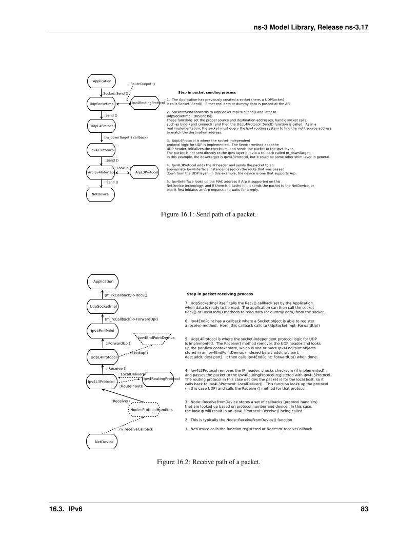
ns-3 Model Library, Release ns-3.17
Figure 16.1: Send path of a packet.
Figure 16.2: Receive path of a packet.
16.3. IPv6 83
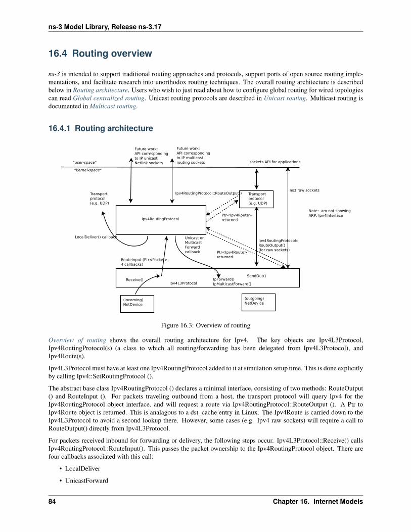
ns-3 Model Library, Release ns-3.17
16.4 Routing overview
ns-3 is intended to support traditional routing approaches and protocols, support ports of open source routing imple-mentations, and facilitate research into unorthodox routing techniques. The overall routing architecture is describedbelow in Routing architecture. Users who wish to just read about how to configure global routing for wired topologiescan read Global centralized routing. Unicast routing protocols are described in Unicast routing. Multicast routing isdocumented in Multicast routing.
16.4.1 Routing architecture
Figure 16.3: Overview of routing
Overview of routing shows the overall routing architecture for Ipv4. The key objects are Ipv4L3Protocol,Ipv4RoutingProtocol(s) (a class to which all routing/forwarding has been delegated from Ipv4L3Protocol), andIpv4Route(s).
Ipv4L3Protocol must have at least one Ipv4RoutingProtocol added to it at simulation setup time. This is done explicitlyby calling Ipv4::SetRoutingProtocol ().
The abstract base class Ipv4RoutingProtocol () declares a minimal interface, consisting of two methods: RouteOutput() and RouteInput (). For packets traveling outbound from a host, the transport protocol will query Ipv4 for theIpv4RoutingProtocol object interface, and will request a route via Ipv4RoutingProtocol::RouteOutput (). A Ptr toIpv4Route object is returned. This is analagous to a dst_cache entry in Linux. The Ipv4Route is carried down to theIpv4L3Protocol to avoid a second lookup there. However, some cases (e.g. Ipv4 raw sockets) will require a call toRouteOutput() directly from Ipv4L3Protocol.
For packets received inbound for forwarding or delivery, the following steps occur. Ipv4L3Protocol::Receive() callsIpv4RoutingProtocol::RouteInput(). This passes the packet ownership to the Ipv4RoutingProtocol object. There arefour callbacks associated with this call:
• LocalDeliver
• UnicastForward
84 Chapter 16. Internet Models
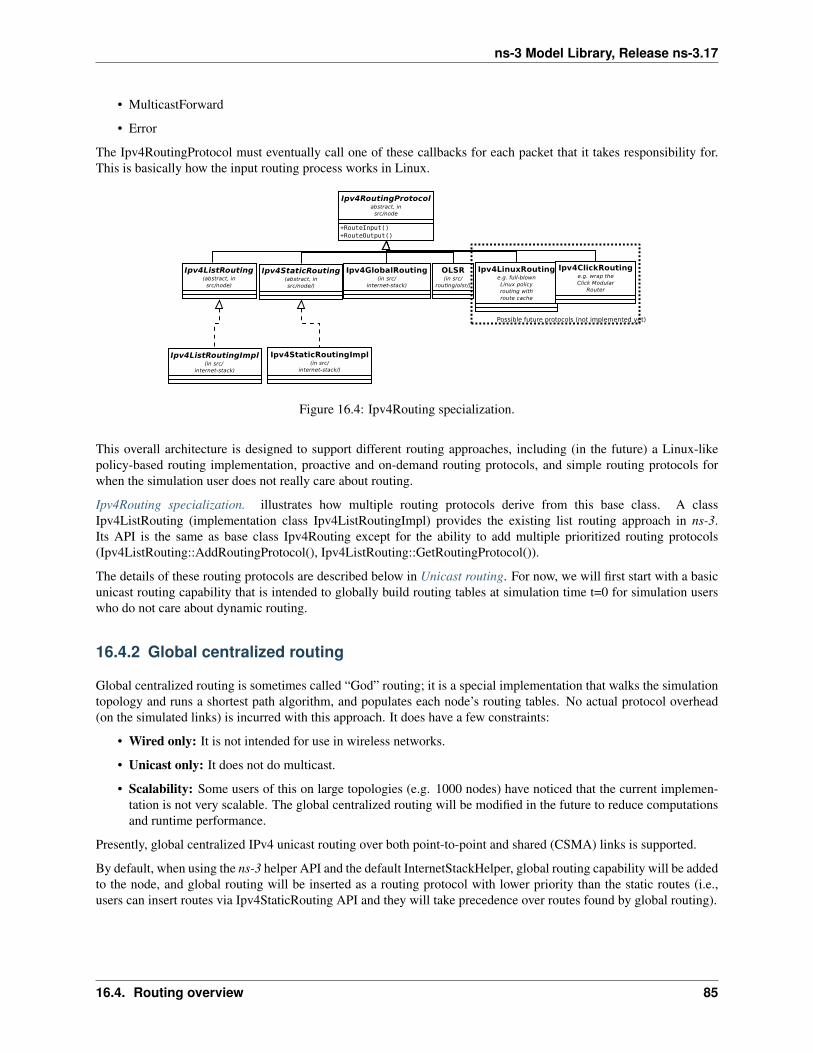
ns-3 Model Library, Release ns-3.17
• MulticastForward
• Error
The Ipv4RoutingProtocol must eventually call one of these callbacks for each packet that it takes responsibility for.This is basically how the input routing process works in Linux.
Figure 16.4: Ipv4Routing specialization.
This overall architecture is designed to support different routing approaches, including (in the future) a Linux-likepolicy-based routing implementation, proactive and on-demand routing protocols, and simple routing protocols forwhen the simulation user does not really care about routing.
Ipv4Routing specialization. illustrates how multiple routing protocols derive from this base class. A classIpv4ListRouting (implementation class Ipv4ListRoutingImpl) provides the existing list routing approach in ns-3.Its API is the same as base class Ipv4Routing except for the ability to add multiple prioritized routing protocols(Ipv4ListRouting::AddRoutingProtocol(), Ipv4ListRouting::GetRoutingProtocol()).
The details of these routing protocols are described below in Unicast routing. For now, we will first start with a basicunicast routing capability that is intended to globally build routing tables at simulation time t=0 for simulation userswho do not care about dynamic routing.
16.4.2 Global centralized routing
Global centralized routing is sometimes called “God” routing; it is a special implementation that walks the simulationtopology and runs a shortest path algorithm, and populates each node’s routing tables. No actual protocol overhead(on the simulated links) is incurred with this approach. It does have a few constraints:
• Wired only: It is not intended for use in wireless networks.
• Unicast only: It does not do multicast.
• Scalability: Some users of this on large topologies (e.g. 1000 nodes) have noticed that the current implemen-tation is not very scalable. The global centralized routing will be modified in the future to reduce computationsand runtime performance.
Presently, global centralized IPv4 unicast routing over both point-to-point and shared (CSMA) links is supported.
By default, when using the ns-3 helper API and the default InternetStackHelper, global routing capability will be addedto the node, and global routing will be inserted as a routing protocol with lower priority than the static routes (i.e.,users can insert routes via Ipv4StaticRouting API and they will take precedence over routes found by global routing).
16.4. Routing overview 85
ns-3 Model Library, Release ns-3.17
Global Unicast Routing API
The public API is very minimal. User scripts include the following::
#include "ns3/internet-module.h"
If the default InternetStackHelper is used, then an instance of global routing will be aggregated to each node. After IPaddresses are configured, the following function call will cause all of the nodes that have an Ipv4 interface to receiveforwarding tables entered automatically by the GlobalRouteManager::
Ipv4GlobalRoutingHelper::PopulateRoutingTables ();
Note: A reminder that the wifi NetDevice will work but does not take any wireless effects into account. For wireless,we recommend OLSR dynamic routing described below.
It is possible to call this function again in the midst of a simulation using the following additional public function::
Ipv4GlobalRoutingHelper::RecomputeRoutingTables ();
which flushes the old tables, queries the nodes for new interface information, and rebuilds the routes.
For instance, this scheduling call will cause the tables to be rebuilt at time 5 seconds::
Simulator::Schedule (Seconds (5),&Ipv4GlobalRoutingHelper::RecomputeRoutingTables);
There are two attributes that govern the behavior. The first is Ipv4GlobalRouting::RandomEcmpRouting. If set to true,packets are randomly routed across equal-cost multipath routes. If set to false (default), only one route is consistentlyused. The second is Ipv4GlobalRouting::RespondToInterfaceEvents. If set to true, dynamically recompute the globalroutes upon Interface notification events (up/down, or add/remove address). If set to false (default), routing may breakunless the user manually calls RecomputeRoutingTables() after such events. The default is set to false to preservelegacy ns-3 program behavior.
Global Routing Implementation
This section is for those readers who care about how this is implemented. A singleton object (GlobalRouteManager)is responsible for populating the static routes on each node, using the public Ipv4 API of that node. It queries eachnode in the topology for a “globalRouter” interface. If found, it uses the API of that interface to obtain a “linkstate advertisement (LSA)” for the router. Link State Advertisements are used in OSPF routing, and we follow theirformatting.
It is important to note that all of these computations are done before packets are flowing in the network. In particular,there are no overhead or control packets being exchanged when using this implementation. Instead, this global routemanager just walks the list of nodes to build the necessary information and configure each node’s routing table.
The GlobalRouteManager populates a link state database with LSAs gathered from the entire topology. Then, foreach router in the topology, the GlobalRouteManager executes the OSPF shortest path first (SPF) computation on thedatabase, and populates the routing tables on each node.
The quagga (http://www.quagga.net) OSPF implementation was used as the basis for the routing computation logic.One benefit of following an existing OSPF SPF implementation is that OSPF already has defined link state advertise-ments for all common types of network links:
• point-to-point (serial links)
• point-to-multipoint (Frame Relay, ad hoc wireless)
• non-broadcast multiple access (ATM)
• broadcast (Ethernet)
86 Chapter 16. Internet Models
ns-3 Model Library, Release ns-3.17
Therefore, we think that enabling these other link types will be more straightforward now that the underlying OSPFSPF framework is in place.
Presently, we can handle IPv4 point-to-point, numbered links, as well as shared broadcast (CSMA) links. Equal-costmultipath is also supported. Although wireless link types are supported by the implementation, note that due to thenature of this implementation, any channel effects will not be considered and the routing tables will assume that everynode on the same shared channel is reachable from every other node (i.e. it will be treated like a broadcast CSMAlink).
The GlobalRouteManager first walks the list of nodes and aggregates a GlobalRouter interface to each one as follows::
typedef std::vector < Ptr<Node> >::iterator Iterator;for (Iterator i = NodeList::Begin (); i != NodeList::End (); i++)
{Ptr<Node> node = *i;Ptr<GlobalRouter> globalRouter = CreateObject<GlobalRouter> (node);node->AggregateObject (globalRouter);
}
This interface is later queried and used to generate a Link State Advertisement for each router, and this link statedatabase is fed into the OSPF shortest path computation logic. The Ipv4 API is finally used to populate the routesthemselves.
16.4.3 Unicast routing
There are presently seven unicast routing protocols defined for IPv4 and two for IPv6:
• class Ipv4StaticRouting (covering both unicast and multicast)
• IPv4 Optimized Link State Routing (OLSR) (a MANET protocol defined in RFC 3626)
• IPv4 Ad Hoc On Demand Distance Vector (AODV) (a MANET protocol defined in RFC 3561)
• IPv4 Destination Sequenced Distance Vector (DSDV) (a MANET protocol)
• class Ipv4ListRouting (used to store a prioritized list of routing protocols)
• class Ipv4GlobalRouting (used to store routes computed by the global route manager, if that is used)
• class Ipv4NixVectorRouting (a more efficient version of global routing that stores source routes in a packetheader field)
• class Ipv6ListRouting (used to store a prioritized list of routing protocols)
• class Ipv6StaticRouting
In the future, this architecture should also allow someone to implement a Linux-like implementation with routingcache, or a Click modular router, but those are out of scope for now.
Ipv4ListRouting
This section describes the current default ns-3 Ipv4RoutingProtocol. Typically, multiple routing protocols are sup-ported in user space and coordinate to write a single forwarding table in the kernel. Presently in ns-3, the implemen-tation instead allows for multiple routing protocols to build/keep their own routing state, and the IPv4 implementationwill query each one of these routing protocols (in some order determined by the simulation author) until a route isfound.
We chose this approach because it may better facilitate the integration of disparate routing approaches that may bedifficult to coordinate the writing to a single table, approaches where more information than destination IP address
16.4. Routing overview 87
ns-3 Model Library, Release ns-3.17
(e.g., source routing) is used to determine the next hop, and on-demand routing approaches where packets must becached.
Ipv4ListRouting::AddRoutingProtocol
Class Ipv4ListRouting provides a pure virtual function declaration for the method that allows one to add a routingprotocol::
void AddRoutingProtocol (Ptr<Ipv4RoutingProtocol> routingProtocol,int16_t priority);
This method is implemented by class Ipv4ListRoutingImpl in the internet-stack module.
The priority variable above governs the priority in which the routing protocols are inserted. Notice that it is asigned int. By default in ns-3, the helper classes will instantiate a Ipv4ListRoutingImpl object, and add to it anIpv4StaticRoutingImpl object at priority zero. Internally, a list of Ipv4RoutingProtocols is stored, and and the routingprotocols are each consulted in decreasing order of priority to see whether a match is found. Therefore, if you wantyour Ipv4RoutingProtocol to have priority lower than the static routing, insert it with priority less than 0; e.g.::
Ptr<MyRoutingProtocol> myRoutingProto = CreateObject<MyRoutingProtocol> ();listRoutingPtr->AddRoutingProtocol (myRoutingProto, -10);
Upon calls to RouteOutput() or RouteInput(), the list routing object will search the list of routing protocols, in priorityorder, until a route is found. Such routing protocol will invoke the appropriate callback and no further routing protocolswill be searched.
Optimized Link State Routing (OLSR)
This IPv4 routing protocol was originally ported from the OLSR-UM implementation for ns-2. The implementationis found in the src/olsr directory, and an example script is in examples/simple-point-to-point-olsr.cc.
Typically, OLSR is enabled in a main program by use of an OlsrHelper class that installs OLSR into anIpv4ListRoutingProtocol object. The following sample commands will enable OLSR in a simulation using this helperclass along with some other routing helper objects. The setting of priority value 10, ahead of the staticRouting priorityof 0, means that OLSR will be consulted for a route before the node’s static routing table.:
NodeContainer c:...// Enable OLSRNS_LOG_INFO ("Enabling OLSR Routing.");OlsrHelper olsr;
Ipv4StaticRoutingHelper staticRouting;
Ipv4ListRoutingHelper list;list.Add (staticRouting, 0);list.Add (olsr, 10);
InternetStackHelper internet;internet.SetRoutingHelper (list);internet.Install (c);
Once installed,the OLSR “main interface” can be set with the SetMainInterface() command. If the user does notspecify a main address, the protocol will select the first primary IP address that it finds, starting first the loopbackinterface and then the next non-loopback interface found, in order of Ipv4 interface index. The loopback address of127.0.0.1 is not selected. In addition, a number of protocol constants are defined in olsr-routing-protocol.cc.
88 Chapter 16. Internet Models
ns-3 Model Library, Release ns-3.17
Olsr is started at time zero of the simulation, based on a call to Object::Start() that eventually calls OlsrRoutingProto-col::DoStart(). Note: a patch to allow the user to start and stop the protocol at other times would be welcome.
Presently, OLSR is limited to use with an Ipv4ListRouting object, and does not respond to dynamic changes to adevice’s IP address or link up/down notifications; i.e. the topology changes are due to loss/gain of connectivity over awireless channel.
16.4.4 Multicast routing
The following function is used to add a static multicast route to a node::
voidIpv4StaticRouting::AddMulticastRoute (Ipv4Address origin,
Ipv4Address group,uint32_t inputInterface,std::vector<uint32_t> outputInterfaces);
A multicast route must specify an origin IP address, a multicast group and an input network interface index as condi-tions and provide a vector of output network interface indices over which packets matching the conditions are sent.
Typically there are two main types of multicast routes: routes of the first kind are used during forwarding. All of theconditions must be explicitly provided. The second kind of routes are used to get packets off of a local node. The differ-ence is in the input interface. Routes for forwarding will always have an explicit input interface specified. Routes off ofa node will always set the input interface to a wildcard specified by the index Ipv4RoutingProtocol::IF_INDEX_ANY.
For routes off of a local node wildcards may be used in the origin and multicast group addresses. The wildcard usedfor Ipv4Adresses is that address returned by Ipv4Address::GetAny () – typically “0.0.0.0”. Usage of a wildcard allowsone to specify default behavior to varying degrees.
For example, making the origin address a wildcard, but leaving the multicast group specific allows one (in the case ofa node with multiple interfaces) to create different routes using different output interfaces for each multicast group.
If the origin and multicast addresses are made wildcards, you have created essentially a default multicast address thatcan forward to multiple interfaces. Compare this to the actual default multicast address that is limited to specifying asingle output interface for compatibility with existing functionality in other systems.
Another command sets the default multicast route::
voidIpv4StaticRouting::SetDefaultMulticastRoute (uint32_t outputInterface);
This is the multicast equivalent of the unicast version SetDefaultRoute. We tell the routing system what to do in thecase where a specific route to a destination multicast group is not found. The system forwards packets out the specifiedinterface in the hope that “something out there” knows better how to route the packet. This method is only used ininitially sending packets off of a host. The default multicast route is not consulted during forwarding – exact routesmust be specified using AddMulticastRoute for that case.
Since we’re basically sending packets to some entity we think may know better what to do, we don’t pay attentionto “subtleties” like origin address, nor do we worry about forwarding out multiple interfaces. If the default multicastroute is set, it is returned as the selected route from LookupStatic irrespective of origin or multicast group if anotherspecific route is not found.
Finally, a number of additional functions are provided to fetch and remove multicast routes::
uint32_t GetNMulticastRoutes (void) const;
Ipv4MulticastRoute *GetMulticastRoute (uint32_t i) const;
Ipv4MulticastRoute *GetDefaultMulticastRoute (void) const;
16.4. Routing overview 89
ns-3 Model Library, Release ns-3.17
bool RemoveMulticastRoute (Ipv4Address origin,Ipv4Address group,uint32_t inputInterface);
void RemoveMulticastRoute (uint32_t index);
16.5 TCP models in ns-3
This chapter describes the TCP models available in ns-3.
16.5.1 Generic support for TCP
ns-3 was written to support multiple TCP implementations. The implementations inherit from a few common headerclasses in the src/network directory, so that user code can swap out implementations with minimal changes to thescripts.
There are two important abstract base classes:
• class TcpSocket: This is defined in src/internet/model/tcp-socket.{cc,h}. This class existsfor hosting TcpSocket attributes that can be reused across different implementations. For instance, the attributeInitialCwnd can be used for any of the implementations that derive from class TcpSocket.
• class TcpSocketFactory: This is used by the layer-4 protocol instance to create TCP sockets of the righttype.
There are presently three implementations of TCP available for ns-3.
• a natively implemented TCP for ns-3
• support for the Network Simulation Cradle (NSC)
• support for Direct Code Exectution (DCE)
It should also be mentioned that various ways of combining virtual machines with ns-3 makes available also someadditional TCP implementations, but those are out of scope for this chapter.
16.5.2 ns-3 TCP
Until ns-3.10 release, ns-3 contained a port of the TCP model from GTNetS. This implementation was substantiallyrewritten by Adriam Tam for ns-3.10. The model is a full TCP, in that it is bidirectional and attempts to model theconnection setup and close logic.
The implementation of TCP is contained in the following files::
src/internet/model/tcp-header.{cc,h}src/internet/model/tcp-l4-protocol.{cc,h}src/internet/model/tcp-socket-factory-impl.{cc,h}src/internet/model/tcp-socket-base.{cc,h}src/internet/model/tcp-tx-buffer.{cc,h}src/internet/model/tcp-rx-buffer.{cc,h}src/internet/model/tcp-rfc793.{cc,h}src/internet/model/tcp-tahoe.{cc,h}src/internet/model/tcp-reno.{cc,h}src/internet/model/tcp-westwood.{cc,h}src/internet/model/tcp-newreno.{cc,h}
90 Chapter 16. Internet Models
ns-3 Model Library, Release ns-3.17
src/internet/model/rtt-estimator.{cc,h}src/network/model/sequence-number.{cc,h}
Different variants of TCP congestion control are supported by subclassing the common base class TcpSocketBase.Several variants are supported, including RFC 793 (no congestion control), Tahoe, Reno, Westwood, Westwood+, andNewReno. NewReno is used by default. See the Usage section of this document for on how to change the default TCPvariant used in simulation.
Usage
In many cases, usage of TCP is set at the application layer by telling the ns-3 application which kind of socket factoryto use.
Using the helper functions defined in src/applications/helper and src/network/helper, here is howone would create a TCP receiver::
// Create a packet sink on the star "hub" to receive these packetsuint16_t port = 50000;Address sinkLocalAddress(InetSocketAddress (Ipv4Address::GetAny (), port));PacketSinkHelper sinkHelper ("ns3::TcpSocketFactory", sinkLocalAddress);ApplicationContainer sinkApp = sinkHelper.Install (serverNode);sinkApp.Start (Seconds (1.0));sinkApp.Stop (Seconds (10.0));
Similarly, the below snippet configures OnOffApplication traffic source to use TCP::
// Create the OnOff applications to send TCP to the serverOnOffHelper clientHelper ("ns3::TcpSocketFactory", Address ());
The careful reader will note above that we have specified the TypeId of an abstract base class TcpSocketFactory.How does the script tell ns-3 that it wants the native ns-3 TCP vs. some other one? Well, when internet stacks are addedto the node, the default TCP implementation that is aggregated to the node is the ns-3 TCP. This can be overridden aswe show below when using Network Simulation Cradle. So, by default, when using the ns-3 helper API, the TCP thatis aggregated to nodes with an Internet stack is the native ns-3 TCP.
To configure behavior of TCP, a number of parameters are exported through the ns-3 attribute system. These aredocumented in the Doxygen <http://www.nsnam.org/doxygen/classns3_1_1_tcp_socket.html> for class TcpSocket.For example, the maximum segment size is a settable attribute.
To set the default socket type before any internet stack-related objects are created, one may put the following statementat the top of the simulation program::
Config::SetDefault ("ns3::TcpL4Protocol::SocketType", StringValue ("ns3::TcpTahoe"));
For users who wish to have a pointer to the actual socket (so that socket operations like Bind(), setting socket options,etc. can be done on a per-socket basis), Tcp sockets can be created by using the Socket::CreateSocket()method. The TypeId passed to CreateSocket() must be of type ns3::SocketFactory, so configuring the un-derlying socket type must be done by twiddling the attribute associated with the underlying TcpL4Protocol object.The easiest way to get at this would be through the attribute configuration system. In the below example, the Nodecontainer “n0n1” is accessed to get the zeroth element, and a socket is created on this node::
// Create and bind the socket...TypeId tid = TypeId::LookupByName ("ns3::TcpTahoe");Config::Set ("/NodeList/*/$ns3::TcpL4Protocol/SocketType", TypeIdValue (tid));Ptr<Socket> localSocket =
Socket::CreateSocket (n0n1.Get (0), TcpSocketFactory::GetTypeId ());
16.5. TCP models in ns-3 91
ns-3 Model Library, Release ns-3.17
Above, the “*” wild card for node number is passed to the attribute configuration system, so that all future sockets onall nodes are set to Tahoe, not just on node ‘n0n1.Get (0)’. If one wants to limit it to just the specified node, one wouldhave to do something like::
// Create and bind the socket...TypeId tid = TypeId::LookupByName ("ns3::TcpTahoe");std::stringstream nodeId;nodeId << n0n1.Get (0)->GetId ();std::string specificNode = "/NodeList/" + nodeId.str () + "/$ns3::TcpL4Protocol/SocketType";Config::Set (specificNode, TypeIdValue (tid));Ptr<Socket> localSocket =
Socket::CreateSocket (n0n1.Get (0), TcpSocketFactory::GetTypeId ());
Once a TCP socket is created, one will want to follow conventional socket logic and either connect() and send() (for aTCP client) or bind(), listen(), and accept() (for a TCP server). See Sockets APIs for a review of how sockets are usedin ns-3.
Validation
Several TCP validation test results can be found in the wiki page describing this implementation.
Current limitations
• SACK is not supported
16.5.3 Network Simulation Cradle
The Network Simulation Cradle (NSC) is a framework for wrapping real-world network code into simulators, allowingsimulation of real-world behavior at little extra cost. This work has been validated by comparing situations using atest network with the same situations in the simulator. To date, it has been shown that the NSC is able to produceextremely accurate results. NSC supports four real world stacks: FreeBSD, OpenBSD, lwIP and Linux. Emphasishas been placed on not changing any of the network stacks by hand. Not a single line of code has been changedin the network protocol implementations of any of the above four stacks. However, a custom C parser was built toprogrammatically change source code.
NSC has previously been ported to ns-2 and OMNeT++, and recently was added to ns-3. This section describes thens-3 port of NSC and how to use it.
Prerequisites
Presently, NSC has been tested and shown to work on these platforms: Linux i386 and Linux x86-64. NSC does notsupport powerpc.
Building NSC requires the packages flex and bison.
Configuring and Downloading
Using the build.py script in ns-3-allinone directory, NSC will be enabled by default unless the platform does notsupport it. To disable it when building ns-3, type::
./waf configure --enable-examples --enable-tests --disable-nsc
92 Chapter 16. Internet Models
ns-3 Model Library, Release ns-3.17
Building and validating
Building ns-3 with nsc support is the same as building it without; no additional arguments are needed for waf. Buildingnsc may take some time compared to ns-3; it is interleaved in the ns-3 building process.
Try running the following ns-3 test suite::
./test.py -s ns3-tcp-interoperability
If NSC has been successfully built, the following test should show up in the results::
PASS TestSuite ns3-tcp-interoperability
This confirms that NSC is ready to use.
Usage
There are a few example files. Try:
./waf --run tcp-nsc-zoo
./waf --run tcp-nsc-lfn
These examples will deposit some .pcap files in your directory, which can be examined by tcpdump or wireshark.
Let’s look at the examples/tcp/tcp-nsc-zoo.cc file for some typical usage. How does it differ from usingnative ns-3 TCP? There is one main configuration line, when using NSC and the ns-3 helper API, that needs to be set::
InternetStackHelper internetStack;
internetStack.SetNscStack ("liblinux2.6.26.so");// this switches nodes 0 and 1 to NSCs Linux 2.6.26 stack.internetStack.Install (n.Get(0));internetStack.Install (n.Get(1));
The key line is the SetNscStack. This tells the InternetStack helper to aggregate instances of NSC TCP instead ofnative ns-3 TCP to the remaining nodes. It is important that this function be called before calling the Install()function, as shown above.
Which stacks are available to use? Presently, the focus has been on Linux 2.6.18 and Linux 2.6.26 stacks for ns-3. Tosee which stacks were built, one can execute the following find command at the ns-3 top level directory::
~/ns-3.10> find nsc -name "*.so" -type fnsc/linux-2.6.18/liblinux2.6.18.sonsc/linux-2.6.26/liblinux2.6.26.so
This tells us that we may either pass the library name liblinux2.6.18.so or liblinux2.6.26.so to the above configurationstep.
Stack configuration
NSC TCP shares the same configuration attributes that are common across TCP sockets, as described above anddocumented in Doxygen
Additionally, NSC TCP exports a lot of configuration variables into the ns-3 attributes system, via a sysctl-like inter-face. In the examples/tcp/tcp-nsc-zoo example, you can see the following configuration::
16.5. TCP models in ns-3 93
ns-3 Model Library, Release ns-3.17
// this disables TCP SACK, wscale and timestamps on node 1 (the attributesrepresent sysctl-values).
Config::Set ("/NodeList/1/$ns3::Ns3NscStack<linux2.6.26>/net.ipv4.tcp_sack",StringValue ("0"));
Config::Set ("/NodeList/1/$ns3::Ns3NscStack<linux2.6.26>/net.ipv4.tcp_timestamps",StringValue ("0"));Config::Set ("/NodeList/1/$ns3::Ns3NscStack<linux2.6.26>/net.ipv4.tcp_window_scaling",StringValue ("0"));
These additional configuration variables are not available to native ns-3 TCP.
Also note that default values for TCP attributes in ns-3 TCP may differ from the nsc TCP implementation. Specificallyin ns-3::
1) TCP default MSS is 5362) TCP Delayed Ack count is 2
Therefore when making comparisons between results obtained using nsc and ns-3 TCP, care must be taken to ensurethese values are set appropriately. See /examples/tcp/tcp-nsc-comparision.cc for an example.
NSC API
This subsection describes the API that NSC presents to ns-3 or any other simulator. NSC provides its API in the formof a number of classes that are defined in sim/sim_interface.h in the nsc directory.
• INetStack INetStack contains the ‘low level’ operations for the operating system network stack, e.g. in andoutput functions from and to the network stack (think of this as the ‘network driver interface’. There are alsofunctions to create new TCP or UDP sockets.
• ISendCallback This is called by NSC when a packet should be sent out to the network. This simulator shoulduse this callback to re-inject the packet into the simulator so the actual data can be delivered/routed to itsdestination, where it will eventually be handed into Receive() (and eventually back to the receivers NSC instancevia INetStack->if_receive() ).
• INetStreamSocket This is the structure defining a particular connection endpoint (file descriptor). It containsmethods to operate on this endpoint, e.g. connect, disconnect, accept, listen, send_data/read_data, ...
• IInterruptCallback This contains the wakeup callback, which is called by NSC whenever something of in-terest happens. Think of wakeup() as a replacement of the operating systems wakeup function: Whenever theoperating system would wake up a process that has been waiting for an operation to complete (for example theTCP handshake during connect()), NSC invokes the wakeup() callback to allow the simulator to check for statechanges in its connection endpoints.
ns-3 implementation
The ns-3 implementation makes use of the above NSC API, and is implemented as follows.
The three main parts are:
• ns3::NscTcpL4Protocol: a subclass of Ipv4L4Protocol (and two nsc classes: ISendCallback and IInter-ruptCallback)
• ns3::NscTcpSocketImpl: a subclass of TcpSocket
• ns3::NscTcpSocketFactoryImpl: a factory to create new NSC sockets
src/internet/model/nsc-tcp-l4-protocol is the main class. Upon Initialization, it loads an nsc networkstack to use (via dlopen()). Each instance of this class may use a different stack. The stack (=shared library) to useis set using the SetNscLibrary() method (at this time its called indirectly via the internet stack helper). The nsc stack
94 Chapter 16. Internet Models

ns-3 Model Library, Release ns-3.17
is then set up accordingly (timers etc). The NscTcpL4Protocol::Receive() function hands the packet it receives (mustbe a complete tcp/ip packet) to the nsc stack for further processing. To be able to send packets, this class implementsthe nsc send_callback method. This method is called by nsc whenever the nsc stack wishes to send a packet out tothe network. Its arguments are a raw buffer, containing a complete TCP/IP packet, and a length value. This methodtherefore has to convert the raw data to a Ptr<Packet> usable by ns-3. In order to avoid various ipv4 header issues, thensc ip header is not included. Instead, the tcp header and the actual payload are put into the Ptr<Packet>, after this thePacket is passed down to layer 3 for sending the packet out (no further special treatment is needed in the send codepath).
This class calls ns3::NscTcpSocketImpl both from the nsc wakeup() callback and from the Receive path (toensure that possibly queued data is scheduled for sending).
src/internet/model/nsc-tcp-socket-impl implements the nsc socket interface. Each instance has itsown nscTcpSocket. Data that is Send() will be handed to the nsc stack via m_nscTcpSocket->send_data(). (andnot to nsc-tcp-l4, this is the major difference compared to ns-3 TCP). The class also queues up data that is Send()before the underlying descriptor has entered an ESTABLISHED state. This class is called from the nsc-tcp-l4 class,when the nsc-tcp-l4 wakeup() callback is invoked by nsc. nsc-tcp-socket-impl then checks the current connection state(SYN_SENT, ESTABLISHED, LISTEN...) and schedules appropriate callbacks as needed, e.g. a LISTEN socket willschedule Accept to see if a new connection must be accepted, an ESTABLISHED socket schedules any pending datafor writing, schedule a read callback, etc.
Note that ns3::NscTcpSocketImpl does not interact with nsc-tcp directly: instead, data is redirected to nsc.nsc-tcp calls the nsc-tcp-sockets of a node when its wakeup callback is invoked by nsc.
Limitations
• NSC only works on single-interface nodes; attempting to run it on a multi-interface node will cause a programerror.
• Cygwin and OS X PPC are not supported
• The non-Linux stacks of NSC are not supported in ns-3
• Not all socket API callbacks are supported
For more information, see this wiki page.
16.5. TCP models in ns-3 95

ns-3 Model Library, Release ns-3.17
96 Chapter 16. Internet Models
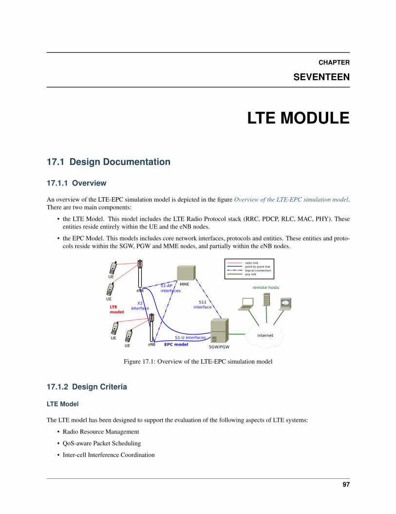
CHAPTER
SEVENTEEN
LTE MODULE
17.1 Design Documentation
17.1.1 Overview
An overview of the LTE-EPC simulation model is depicted in the figure Overview of the LTE-EPC simulation model.There are two main components:
• the LTE Model. This model includes the LTE Radio Protocol stack (RRC, PDCP, RLC, MAC, PHY). Theseentities reside entirely within the UE and the eNB nodes.
• the EPC Model. This models includes core network interfaces, protocols and entities. These entities and proto-cols reside within the SGW, PGW and MME nodes, and partially within the eNB nodes.
Figure 17.1: Overview of the LTE-EPC simulation model
17.1.2 Design Criteria
LTE Model
The LTE model has been designed to support the evaluation of the following aspects of LTE systems:
• Radio Resource Management
• QoS-aware Packet Scheduling
• Inter-cell Interference Coordination
97
ns-3 Model Library, Release ns-3.17
• Dynamic Spectrum Access
In order to model LTE systems to a level of detail that is sufficient to allow a correct evaluation of the above mentionedaspects, the following requirements have been considered:
1. At the radio level, the granularity of the model should be at least that of the Resource Block (RB). In fact,this is the fundamental unit being used for resource allocation. Without this minimum level of granularity, it isnot possible to model accurately packet scheduling and inter-cell-interference. The reason is that, since packetscheduling is done on a per-RB basis, an eNB might transmit on a subset only of all the available RBs, henceinterfering with other eNBs only on those RBs where it is trasmitting. Note that this requirement rules out theadoption of a system level simulation approach, which evaluates resource allocation only at the granularity ofcall/bearer establishment.
2. The simulator should scale up to tens of eNBs and hundreds of User Equipments (UEs). This rules out the use ofa link level simulator, i.e., a simulator whose radio interface is modeled with a granularity up to the symbol level.This is because to have a symbol level model it is necessary to implement all the PHY layer signal processing,whose huge computational complexity severely limits simulation. In fact, link-level simulators are normallylimited to a single eNB and one or a few UEs.
3. It should be possible within the simulation to configure different cells so that they use different carrier frequen-cies and system bandwidths. The bandwidth used by different cells should be allowed to overlap, in order tosupport dynamic spectrum licensing solutions such as those described in [Ofcom2600MHz] and [RealWireless].The calculation of interference should handle appropriately this case.
4. To be more representative of the LTE standard, as well as to be as close as possible to real-world implemen-tations, the simulator should support the MAC Scheduler API published by the FemtoForum [FFAPI]. Thisinterface is expected to be used by femtocell manufacturers for the implementation of scheduling and RadioResource Management (RRM) algorithms. By introducing support for this interface in the simulator, we makeit possible for LTE equipment vendors and operators to test in a simulative environment exactly the same algo-rithms that would be deployed in a real system.
5. The LTE simulation model should contain its own implementation of the API defined in [FFAPI]. Neitherbinary nor data structure compatibility with vendor-specific implementations of the same interface are expected;hence, a compatibility layer should be interposed whenever a vendor-specific MAC scheduler is to be used withthe simulator. This requirement is necessary to allow the simulator to be independent from vendor-specificimplementations of this interface specification. We note that [FFAPI] is a logical specification only, and itsimplementation (e.g., translation to some specific programming language) is left to the vendors.
6. The model is to be used to simulate the transmission of IP packets by the upper layers. With this respect, itshall be considered that in LTE the Scheduling and Radio Resource Management do not work with IP packetsdirectly, but rather with RLC PDUs, which are obtained by segmentation and concatenation of IP packets doneby the RLC entities. Hence, these functionalities of the RLC layer should be modeled accurately.
EPC Model
The main objective of the EPC model is to provides means for the simulation of end-to-end IP connectivity over theLTE model. To this aim, it supports for the interconnection of multiple UEs to the internet, via a radio access networkof multiple eNBs connected to a single SGW/PGW node, as shown in Figure Overview of the LTE-EPC simulationmodel.
The following design choices have been made for the EPC model:
1. The only Packet Data Network (PDN) type supported is IPv4.
2. The SGW and PGW functional entities are implemented within a single node, which is hence referred to as theSGW/PGW node.
3. The scenarios with inter-SGW mobility are not of interests. Hence, a single SGW/PGW node will be present inall simulations scenarios
98 Chapter 17. LTE Module
ns-3 Model Library, Release ns-3.17
4. A requirement for the EPC model is that it can be used to simulate the end-to-end performance of realisticapplications. Hence, it should be possible to use with the EPC model any regular ns-3 application working ontop of TCP or UDP.
5. Another requirement is the possibility of simulating network topologies with the presence of multiple eNBs,some of which might be equipped with a backhaul connection with limited capabilities. In order to simulatesuch scenarios, the user data plane protocols being used between the eNBs and the SGW/PGW should bemodeled accurately.
6. It should be possible for a single UE to use different applications with different QoS profiles. Hence, multipleEPS bearers should be supported for each UE. This includes the necessary classification of TCP/UDP trafficover IP done at the UE in the uplink and at the PGW in the downlink.
7. The focus of the EPC model is mainly on the EPC data plane. The accurate modeling of the EPC control planeis, for the time being, not a requirement; hence, the necessary control plane interactions can be modeled in asimplified way by leveraging on direct interaction among the different simulation objects via the provided helperobjects.
8. The focus of the EPC model is on simulations of active users in ECM connected mode. Hence, all the function-ality that is only relevant for ECM idle mode (in particular, tracking area update and paging) are not modeled atall.
9. The model should allow the possibility to perform an X2-based handover between two eNBs.
17.1.3 Architecture
LTE Model
UE architecture
The architecture of the LTE radio protocol stack model of the UE is represented in the figures LTE radio protocol stackarchitecture for the UE on the data plane and LTE radio protocol stack architecture for the UE on the control planewhich highlight respectively the data plane and the control plane.
The architecture of the PHY/channel model of the UE is represented in figure PHY and channel model architecturefor the UE.
eNB architecture
The architecture of the LTE radio protocol stack model of the eNB is represented in the figures LTE radio protocolstack architecture for the eNB on the data plane and LTE radio protocol stack architecture for the eNB on the controlplane which highlight respectively the data plane and the control plane.
The architecture of the PHY/channel model of the eNB is represented in figure PHY and channel model architecturefor the eNB.
EPC Model
EPC data plane
In Figure LTE-EPC data plane protocol stack, we represent the end-to-end LTE-EPC data plane protocol stack as itis modeled in the simulator. From the figure, it is evident that the biggest simplification introduced in the data planemodel is the inclusion of the SGW and PGW functionality within a single SGW/PGW node, which removes the need
17.1. Design Documentation 99
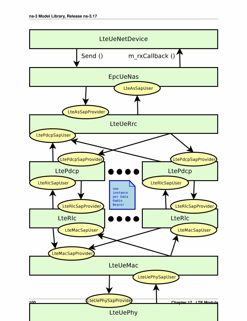
ns-3 Model Library, Release ns-3.17
Figure 17.2: LTE radio protocol stack architecture for the UE on the data plane
100 Chapter 17. LTE Module
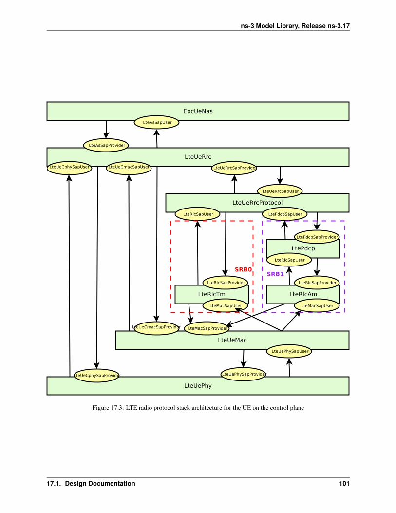
ns-3 Model Library, Release ns-3.17
Figure 17.3: LTE radio protocol stack architecture for the UE on the control plane
17.1. Design Documentation 101
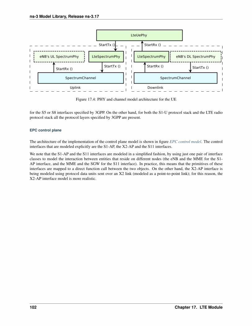
ns-3 Model Library, Release ns-3.17
Figure 17.4: PHY and channel model architecture for the UE
for the S5 or S8 interfaces specified by 3GPP. On the other hand, for both the S1-U protocol stack and the LTE radioprotocol stack all the protocol layers specified by 3GPP are present.
EPC control plane
The architecture of the implementation of the control plane model is shown in figure EPC control model. The controlinterfaces that are modeled explicitly are the S1-AP, the X2-AP and the S11 interfaces.
We note that the S1-AP and the S11 interfaces are modeled in a simplified fashion, by using just one pair of interfaceclasses to model the interaction between entities that reside on different nodes (the eNB and the MME for the S1-AP interface, and the MME and the SGW for the S11 interface). In practice, this means that the primitives of theseinterfaces are mapped to a direct function call between the two objects. On the other hand, the X2-AP interface isbeing modeled using protocol data units sent over an X2 link (modeled as a point-to-point link); for this reason, theX2-AP interface model is more realistic.
102 Chapter 17. LTE Module
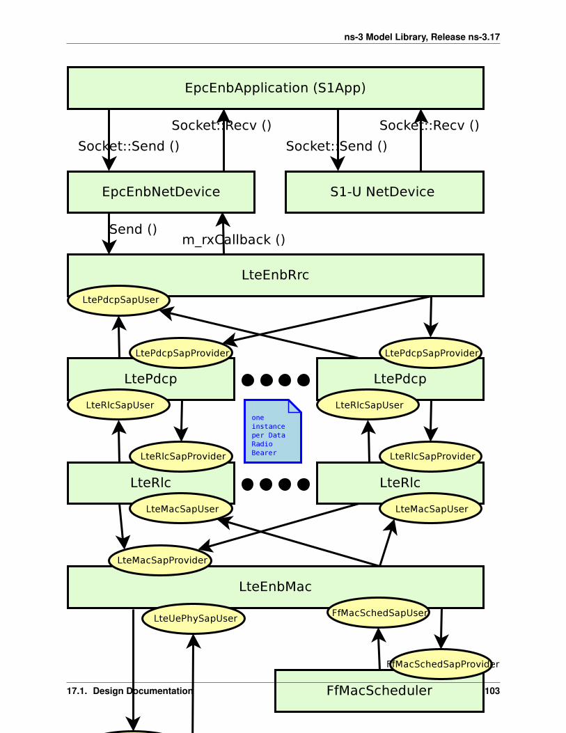
ns-3 Model Library, Release ns-3.17
Figure 17.5: LTE radio protocol stack architecture for the eNB on the data plane
17.1. Design Documentation 103
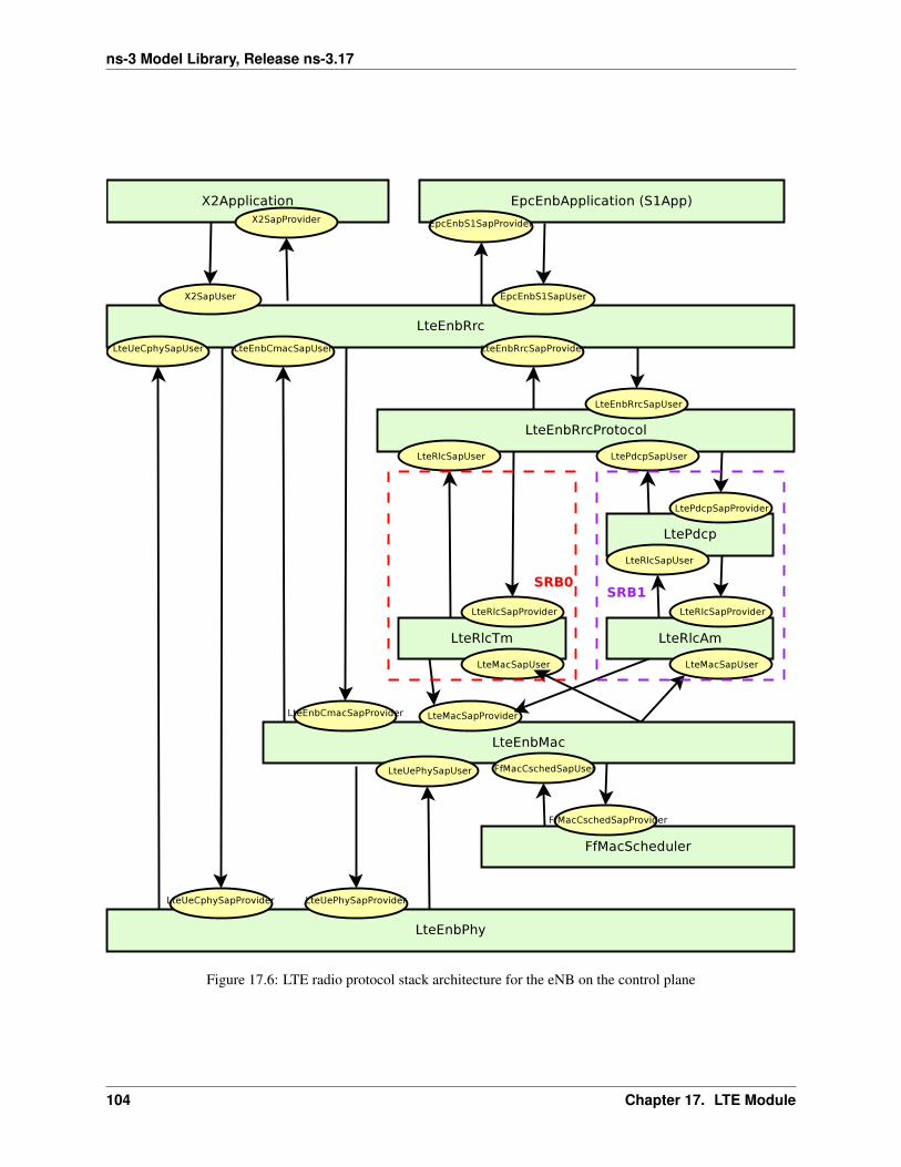
ns-3 Model Library, Release ns-3.17
Figure 17.6: LTE radio protocol stack architecture for the eNB on the control plane
104 Chapter 17. LTE Module
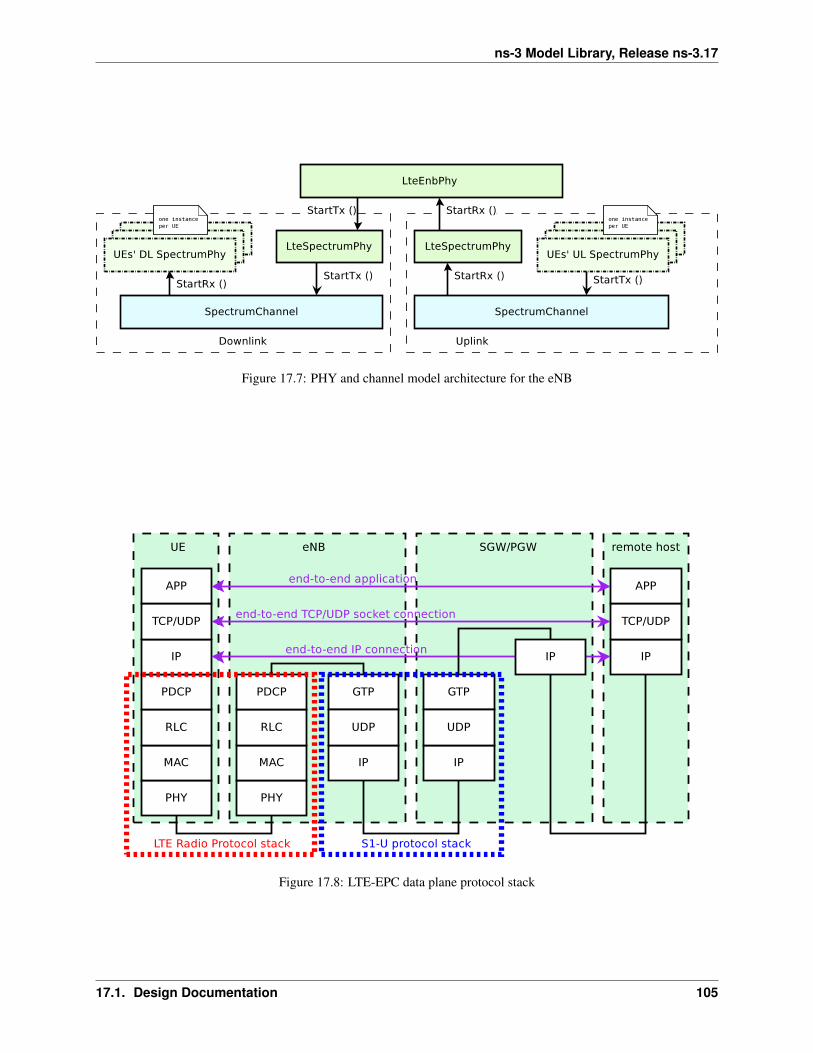
ns-3 Model Library, Release ns-3.17
Figure 17.7: PHY and channel model architecture for the eNB
Figure 17.8: LTE-EPC data plane protocol stack
17.1. Design Documentation 105
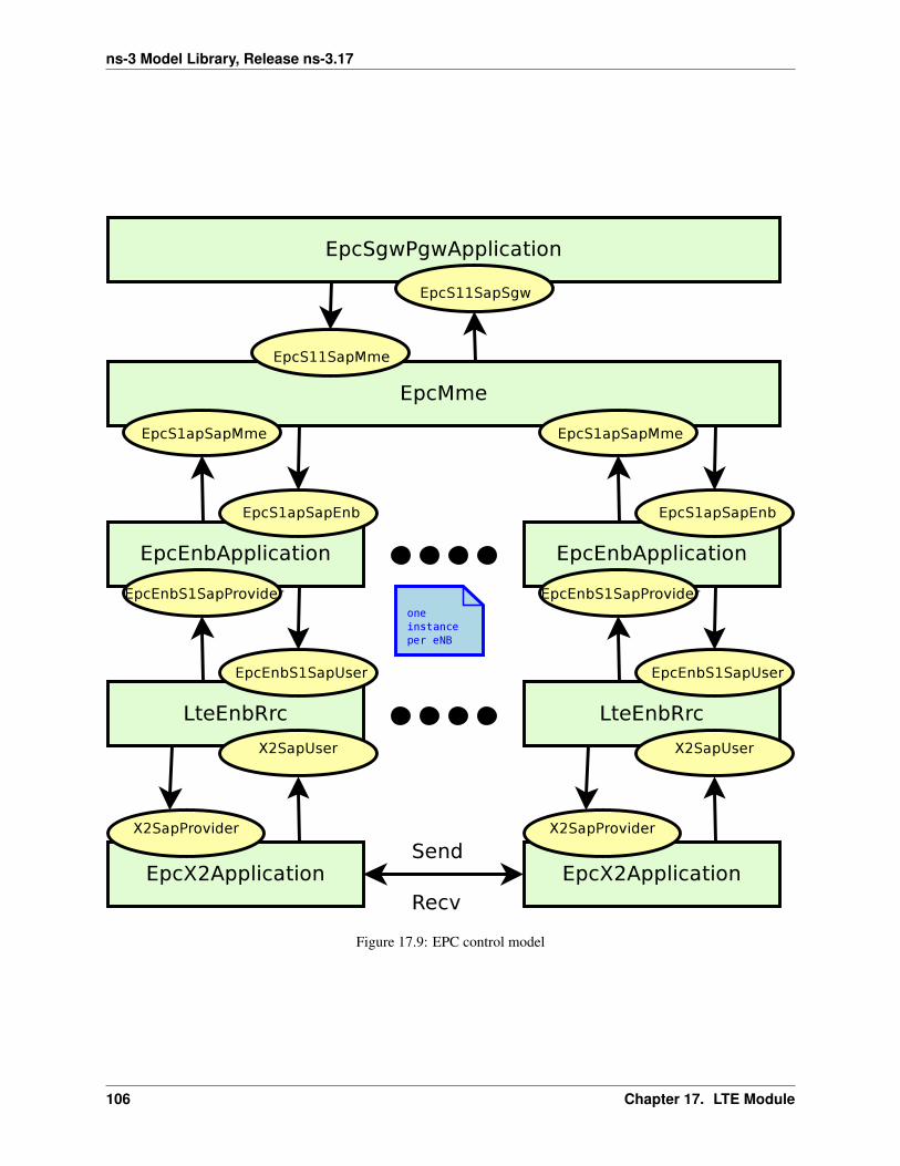
ns-3 Model Library, Release ns-3.17
Figure 17.9: EPC control model
106 Chapter 17. LTE Module

ns-3 Model Library, Release ns-3.17
17.1.4 Channel and Propagation
For channel modeling purposes, the LTE module uses the SpectrumChannel interface provided by thespectrum module. At the time of this writing, two implementations of such interface are available:SingleModelSpectrumChannel and MultiModelSpectrumChannel, and the LTE module requiresthe use of the MultiModelSpectrumChannel in order to work properly. This is because of the needto support different frequency and bandwidth configurations. All the the propagation models supported byMultiModelSpectrumChannel can be used within the LTE module.
Use of the Buildings model with LTE
The recommended propagation model to be used with the LTE module is the one provided by the Buildings mod-ule, which was in fact designed specifically with LTE (though it can be used with other wireless technologies aswell). Please refer to the documentation of the Buildings module for generic information on the propagation model itprovides.
In this section we will highlight some considerations that specifically apply when the Buildings module is used togetherwith the LTE module.
The naming convention used in the following will be:
• User equipment: UE
• Macro Base Station: MBS
• Small cell Base Station (e.g., pico/femtocell): SC
The LTE module considers FDD only, and implements downlink and uplink propagation separately. As a consequence,the following pathloss computations are performed
• MBS <-> UE (indoor and outdoor)
• SC (indoor and outdoor) <-> UE (indoor and outdoor)
The LTE model does not provide the following pathloss computations:
• UE <-> UE
• MBS <-> MBS
• MBS <-> SC
• SC <-> SC
The Buildings model does not know the actual type of the node; i.e., it is not aware of whether a transmitter node is aUE, a MBS, or a SC. Rather, the Buildings model only cares about the position of the node: whether it is indoor andoutdoor, and what is its z-axis respect to the rooftop level. As a consequence, for an eNB node that is placed outdoorand at a z-coordinate above the rooftop level, the propagation models typical of MBS will be used by the Buildingsmodule. Conversely, for an eNB that is placed outdoor but below the rooftop, or indoor, the propagation models typicalof pico and femtocells will be used.
For communications involving at least one indoor node, the corresponding wall penetration losses will be calculatedby the Buildings model. This covers the following use cases:
• MBS <-> indoor UE
• outdoor SC <-> indoor UE
• indoor SC <-> indoor UE
• indoor SC <-> outdoor UE
Please refer to the documentation of the Buildings module for details on the actual models used in each case.
17.1. Design Documentation 107

ns-3 Model Library, Release ns-3.17
Fading Model
The LTE module includes a trace-based fading model derived from the one developed during the GSoC 2010[Piro2011]. The main characteristic of this model is the fact that the fading evaluation during simulation run-timeis based on per-calculated traces. This is done to limit the computational complexity of the simulator. On the otherhand, it needs huge structures for storing the traces; therefore, a trade-off between the number of possible parametersand the memory occupancy has to be found. The most important ones are:
• users’ speed: relative speed between users (affects the Doppler frequency, which in turns affects the time-variance property of the fading)
• number of taps (and relative power): number of multiple paths considered, which affects the frequency propertyof the fading.
• time granularity of the trace: sampling time of the trace.
• frequency granularity of the trace: number of values in frequency to be evaluated.
• length of trace: ideally large as the simulation time, might be reduced by windowing mechanism.
• number of users: number of independent traces to be used (ideally one trace per user).
With respect to the mathematical channel propagation model, we suggest the one provided by the rayleighchanfunction of Matlab, since it provides a well accepted channel modelization both in time and frequency domain. Formore information, the reader is referred to [mathworks].
The simulator provides a matlab script (/lte/model/JakesTraces/fading-trace-generator.m) forgenerating traces based on the format used by the simulator. In detail, the channel object created with the rayleighchanfunction is used for filtering a discrete-time impulse signal in order to obtain the channel impulse response. Thefiltering is repeated for different TTI, thus yielding subsequent time-correlated channel responses (one per TTI). Thechannel response is then processed with the pwelch function for obtaining its power spectral density values, whichare then saved in a file with the proper format compatible with the simulator model.
Since the number of variable it is pretty high, generate traces considering all of them might produce a high numberof traces of huge size. On this matter, we considered the following assumptions of the parameters based on the 3GPPfading propagation conditions (see Annex B.2 of [TS36104]):
• users’ speed: typically only a few discrete values are considered, i.e.:
– 0 and 3 kmph for pedestrian scenarios
– 30 and 60 kmph for vehicular scenarios
– 0, 3, 30 and 60 for urban scenarios
• channel taps: only a limited number of sets of channel taps are normally considered, for example three modelsare mentioned in Annex B.2 of [TS36104].
• time granularity: we need one fading value per TTI, i.e., every 1 ms (as this is the granularity in time of the ns-3LTE PHY model).
• frequency granularity: we need one fading value per RB (which is the frequency granularity of the spectrummodel used by the ns-3 LTE model).
• length of the trace: the simulator includes the windowing mechanism implemented during the GSoC 2011,which consists of picking up a window of the trace each window length in a random fashion.
• per-user fading process: users share the same fading trace, but for each user a different starting point in the traceis randomly picked up. This choice was made to avoid the need to provide one fading trace per user.
108 Chapter 17. LTE Module

ns-3 Model Library, Release ns-3.17
According to the parameters we considered, the following formula express in detail the total size Straces of the fadingtraces:
Straces = Ssample ×NRB ×TtraceTsample
×Nscenarios [bytes]
where Ssample is the size in bytes of the sample (e.g., 8 in case of double precision, 4 in case of float precision), NRBis the number of RB or set of RBs to be considered, Ttrace is the total length of the trace, Tsample is the time resolutionof the trace (1 ms), and Nscenarios is the number of fading scenarios that are desired (i.e., combinations of differentsets of channel taps and user speed values). We provide traces for 3 different scenarios one for each taps configurationdefined in Annex B.2 of [TS36104]:
• Pedestrian: with nodes’ speed of 3 kmph.
• Vehicular: with nodes’ speed of 60 kmph.
• Urban: with nodes’ speed of 3 kmph.
hence Nscenarios = 3. All traces have Ttrace = 10 s and RBNUM = 100. This results in a total 24 MB bytes oftraces.
Antennas
Being based on the SpectrumPhy, the LTE PHY model supports antenna modeling via the ns-3 AntennaModel class.Hence, any model based on this class can be associated with any eNB or UE instance. For instance, the use of theCosineAntennaModel associated with an eNB device allows to model one sector of a macro base station. By default,the IsotropicAntennaModel is used for both eNBs and UEs.
17.1. Design Documentation 109
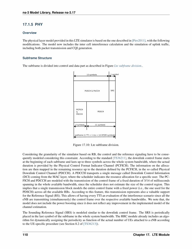
ns-3 Model Library, Release ns-3.17
17.1.5 PHY
Overview
The physical layer model provided in this LTE simulator is based on the one described in [Piro2011], with the followingmodifications. The model now includes the inter cell intereference calculation and the simulation of uplink traffic,including both packet transmission and CQI generation.
Subframe Structure
The subframe is divided into control and data part as described in Figure Lte subframe division..
Figure 17.10: Lte subframe division.
Considering the granularity of the simulator based on RB, the control and the reference signaling have to be conse-quently modeled considering this constraint. According to the standard [TS36211], the downlink control frame startsat the beginning of each subframe and lasts up to three symbols across the whole system bandwidth, where the actualduration is provided by the Physical Control Format Indicator Channel (PCFICH). The information on the alloca-tion are then mapped in the remaining resource up to the duration defined by the PCFICH, in the so called PhysicalDownlink Control Channel (PDCCH). A PDCCH transports a single message called Downlink Control Information(DCI) coming from the MAC layer, where the scheduler indicates the resource allocation for a specific user. The PC-FICH and PDCCH are modeled with the transmission of the control frame of a fixed duration of 3/14 of millisecondsspanning in the whole available bandwidth, since the scheduler does not estimate the size of the control region. Thisimplies that a single transmission block models the entire control frame with a fixed power (i.e., the one used for thePDSCH) across all the available RBs. According to this feature, this transmission represents also a valuable supportfor the Reference Signal (RS). This allows of having every TTI an evaluation of the interference scenario since all theeNB are transmitting (simultaneously) the control frame over the respective available bandwidths. We note that, themodel does not include the power boosting since it does not reflect any improvement in the implemented model of thechannel estimation.
The Sounding Reference Signal (SRS) is modeled similar to the downlink control frame. The SRS is periodicallyplaced in the last symbol of the subframe in the whole system bandwidth. The RRC module already includes an algo-rithm for dynamically assigning the periodicity as function of the actual number of UEs attached to a eNB accordingto the UE-specific procedure (see Section 8.2 of [TS36213]).
110 Chapter 17. LTE Module
ns-3 Model Library, Release ns-3.17
MAC to Channel delay
To model the latency of real MAC and PHY implementations, the PHY model simulates a MAC-to-channel delay inmultiples of TTIs (1ms). The transmission of both data and control packets are delayed by this amount.
CQI feedback
The generation of CQI feedback is done accordingly to what specified in [FFAPI]. In detail, we considered the gener-ation of periodic wideband CQI (i.e., a single value of channel state that is deemed representative of all RBs in use)and inband CQIs (i.e., a set of value representing the channel state for each RB).
In downlink, the CQI feedbacks are currently evaluated according to the SINR perceived by control channel (i.e.,PDCCH + PCFIC) in order to have an estimation of the interference when all the eNB are transmitting simultaneously.In uplink, two types of CQIs are implemented:
• SRS based, periodically sent by the UEs.
• PUSCH based, calculated from the actual transmitted data.
The scheduler interface include an attribute system calld UlCqiFilter for managing the filtering of the CQIsaccording to their nature, in detail:
• SRS_UL_CQI for storing only SRS based CQIs.
• PUSCH_UL_CQI for storing only PUSCH based CQIs.
• ALL_UL_CQI for storing all the CQIs received.
It has to be noted that, the FfMacScheduler provides only the interface and it is matter of the actual schedulerimplementation to include the code for managing these attibutes (see scheduler related section for more informationon this matter).
Interference Model
The PHY model is based on the well-known Gaussian interference models, according to which the powers of interfer-ing signals (in linear units) are summed up together to determine the overall interference power.
The sequence diagram of Figure Sequence diagram of the PHY interference calculation procedure shows how inter-fering signals are processed to calculate the SINR, and how SINR is then used for the generation of CQI feedback.
LTE Spectrum Model
The usage of the radio spectrum by eNBs and UEs in LTE is described in [TS36101]. In the simulator, radio spectrumusage is modeled as follows. Let fc denote the LTE Absolute Radio Frequency Channel Number, which identifies thecarrier frequency on a 100 kHz raster; furthermore, let B be the Transmission Bandwidth Configuration in numberof Resource Blocks. For every pair (fc, B) used in the simulation we define a corresponding spectrum model usingthe Spectrum framework described in [Baldo2009]. fc and B can be configured for every eNB instantiated in thesimulation; hence, each eNB can use a different spectrum model. Every UE will automatically use the spectrummodel of the eNB it is attached to. Using the MultiModelSpectrumChannel described in [Baldo2009], the interferenceamong eNBs that use different spectrum models is properly accounted for. This allows to simulate dynamic spectrumaccess policies, such as for example the spectrum licensing policies that are discussed in [Ofcom2600MHz].
17.1. Design Documentation 111
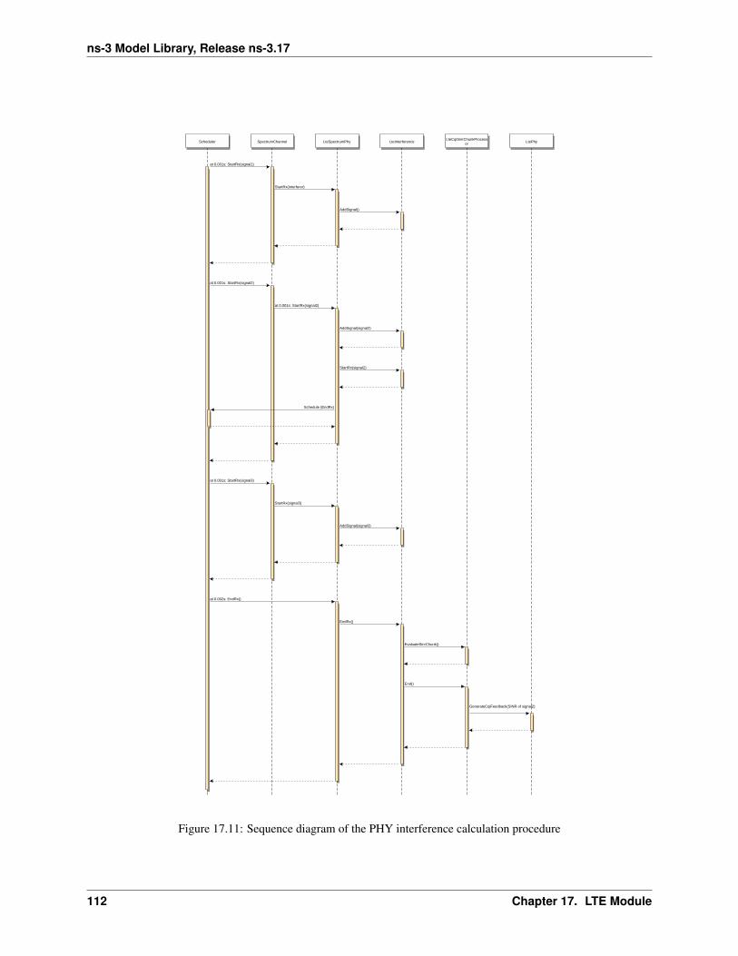
ns-3 Model Library, Release ns-3.17
Scheduler SpectrumChannel LteSpectrumPhy LteInterferenceLteCqiSinrChunkProcess
or LtePhy
at 0.001s: StartRx(signal1)
StartRx(interferer)
AddSignal()
at 0.001s: StartRx(signal2)
at 0.001s: StartRx(signal2)
AddSignal(signal2)
StartRx(signal2)
Schedule (EndRx)
at 0.001s: StartRx(signal3)
StartRx(signal3)
AddSignal(signal3)
at 0.002s: EndRx()
EndRx()
EvaluateSinrChunk()
End()
GenerateCqiFeedback(SINR of signal2)
Figure 17.11: Sequence diagram of the PHY interference calculation procedure
112 Chapter 17. LTE Module
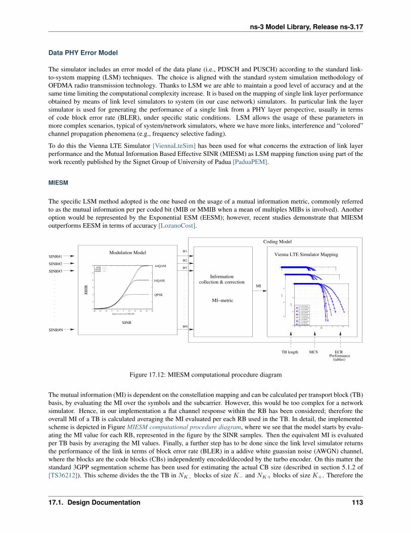
ns-3 Model Library, Release ns-3.17
Data PHY Error Model
The simulator includes an error model of the data plane (i.e., PDSCH and PUSCH) according to the standard link-to-system mapping (LSM) techniques. The choice is aligned with the standard system simulation methodology ofOFDMA radio transmission technology. Thanks to LSM we are able to maintain a good level of accuracy and at thesame time limiting the computational complexity increase. It is based on the mapping of single link layer performanceobtained by means of link level simulators to system (in our case network) simulators. In particular link the layersimulator is used for generating the performance of a single link from a PHY layer perspective, usually in termsof code block error rate (BLER), under specific static conditions. LSM allows the usage of these parameters inmore complex scenarios, typical of system/network simulators, where we have more links, interference and “colored”channel propagation phenomena (e.g., frequency selective fading).
To do this the Vienna LTE Simulator [ViennaLteSim] has been used for what concerns the extraction of link layerperformance and the Mutual Information Based Effective SINR (MIESM) as LSM mapping function using part of thework recently published by the Signet Group of University of Padua [PaduaPEM].
MIESM
The specific LSM method adopted is the one based on the usage of a mutual information metric, commonly referredto as the mutual information per per coded bit (MIB or MMIB when a mean of multiples MIBs is involved). Anotheroption would be represented by the Exponential ESM (EESM); however, recent studies demonstrate that MIESMoutperforms EESM in terms of accuracy [LozanoCost].
0 1 2 3 4 5 6 7 810
−3
10−2
10−1
100
SNR
BLE
R
TB = 6000 (AWGN)
TB = 6000 (estimated)
TB = 4000 (AWGN)
TB = 4000 (estimated)
TB = 2560 (AWGN)
TB = 2560 (estimated)
TB = 1024 (AWGN)
TB = 1024 (estimated)
TB = 512 (AWGN)
TB = 512 (estimated)
TB = 256 (AWGN)
TB = 256 (estimated)
TB = 160 (AWGN)
TB = 160 (estimated)
0
1
2
3
4
5
6
-20 -15 -10 -5 0 5 10 15 20 25 30
RB
IR
Signal-to-noise ratio SNR [dB]
QPSK16QAM64QAM
4 4.5 5 5.5 6 6.5 7 7.5 8 8.5 910
−3
10−2
10−1
100
SNR
BLE
R
TB = 6000 (AWGN)
TB = 6000 (estimated)
TB = 4000 (AWGN)
TB = 4000 (estimated)
TB = 2560 (AWGN)
TB = 2560 (estimated)
TB = 1024 (AWGN)
TB = 1024 (estimated)
TB = 512 (AWGN)
TB = 512 (estimated)
TB = 256 (AWGN)
TB = 256 (estimated)
4 4.5 5 5.5 6 6.5 7 7.5 8 8.5 910
−3
10−2
10−1
100
SNR
BLE
R
TB = 6000 (AWGN)
TB = 6000 (estimated)
TB = 4000 (AWGN)
TB = 4000 (estimated)
TB = 2560 (AWGN)
TB = 2560 (estimated)
TB = 1024 (AWGN)
TB = 1024 (estimated)
TB = 512 (AWGN)
TB = 512 (estimated)
TB = 256 (AWGN)
TB = 256 (estimated)
SINR#1
SINR#2
SINR#3
SINR#N
I#1
I#2
I#3
Modulation Model
Informationcollection & correction
MI−metric
MI
TB length MCS ECRPerformance
(tables)
Coding Model
I#N
64QAM
Vienna LTE Simulator Mapping
16QAM
QPSK
SINR
RB
IR
Figure 17.12: MIESM computational procedure diagram
The mutual information (MI) is dependent on the constellation mapping and can be calculated per transport block (TB)basis, by evaluating the MI over the symbols and the subcarrier. However, this would be too complex for a networksimulator. Hence, in our implementation a flat channel response within the RB has been considered; therefore theoverall MI of a TB is calculated averaging the MI evaluated per each RB used in the TB. In detail, the implementedscheme is depicted in Figure MIESM computational procedure diagram, where we see that the model starts by evalu-ating the MI value for each RB, represented in the figure by the SINR samples. Then the equivalent MI is evaluatedper TB basis by averaging the MI values. Finally, a further step has to be done since the link level simulator returnsthe performance of the link in terms of block error rate (BLER) in a addive white guassian noise (AWGN) channel,where the blocks are the code blocks (CBs) independently encoded/decoded by the turbo encoder. On this matter thestandard 3GPP segmentation scheme has been used for estimating the actual CB size (described in section 5.1.2 of[TS36212]). This scheme divides the the TB in NK− blocks of size K− and NK+ blocks of size K+. Therefore the
17.1. Design Documentation 113
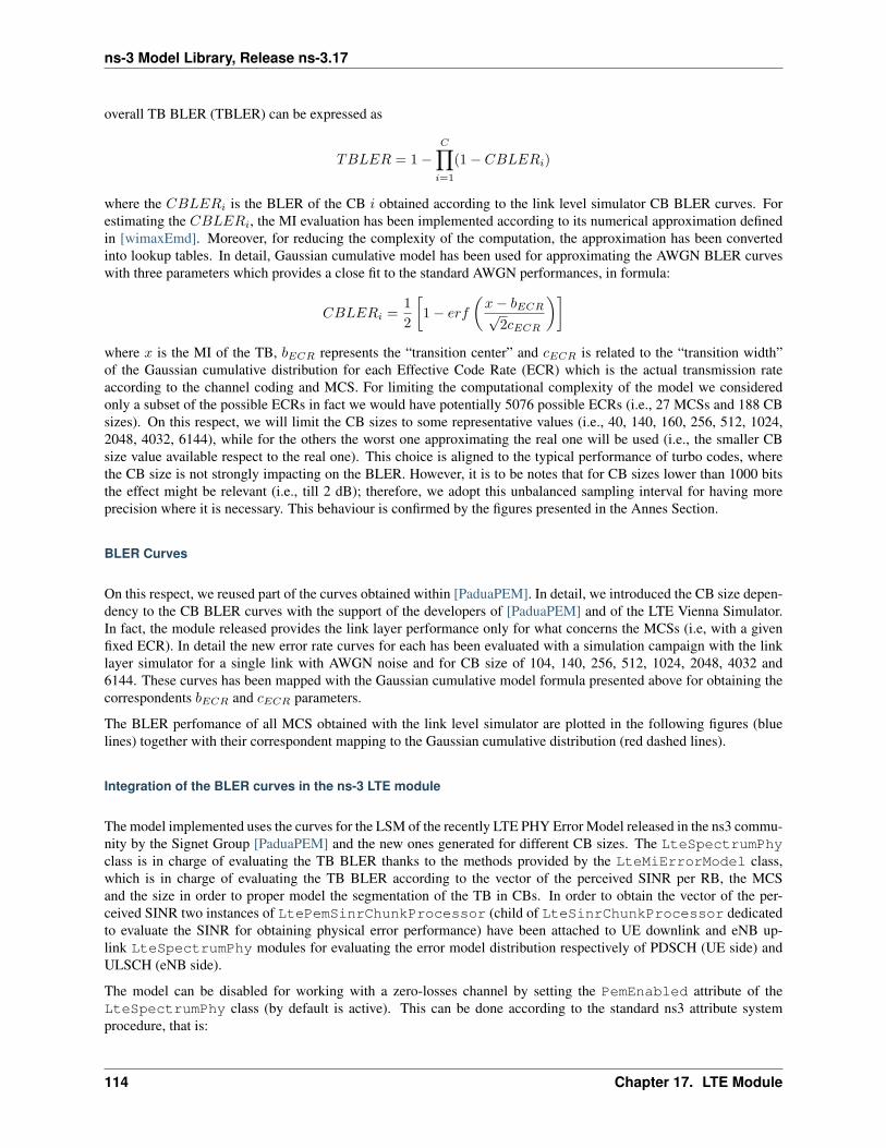
ns-3 Model Library, Release ns-3.17
overall TB BLER (TBLER) can be expressed as
TBLER = 1−C∏i=1
(1− CBLERi)
where the CBLERi is the BLER of the CB i obtained according to the link level simulator CB BLER curves. Forestimating the CBLERi, the MI evaluation has been implemented according to its numerical approximation definedin [wimaxEmd]. Moreover, for reducing the complexity of the computation, the approximation has been convertedinto lookup tables. In detail, Gaussian cumulative model has been used for approximating the AWGN BLER curveswith three parameters which provides a close fit to the standard AWGN performances, in formula:
CBLERi =12
[1− erf
(x− bECR√
2cECR
)]where x is the MI of the TB, bECR represents the “transition center” and cECR is related to the “transition width”of the Gaussian cumulative distribution for each Effective Code Rate (ECR) which is the actual transmission rateaccording to the channel coding and MCS. For limiting the computational complexity of the model we consideredonly a subset of the possible ECRs in fact we would have potentially 5076 possible ECRs (i.e., 27 MCSs and 188 CBsizes). On this respect, we will limit the CB sizes to some representative values (i.e., 40, 140, 160, 256, 512, 1024,2048, 4032, 6144), while for the others the worst one approximating the real one will be used (i.e., the smaller CBsize value available respect to the real one). This choice is aligned to the typical performance of turbo codes, wherethe CB size is not strongly impacting on the BLER. However, it is to be notes that for CB sizes lower than 1000 bitsthe effect might be relevant (i.e., till 2 dB); therefore, we adopt this unbalanced sampling interval for having moreprecision where it is necessary. This behaviour is confirmed by the figures presented in the Annes Section.
BLER Curves
On this respect, we reused part of the curves obtained within [PaduaPEM]. In detail, we introduced the CB size depen-dency to the CB BLER curves with the support of the developers of [PaduaPEM] and of the LTE Vienna Simulator.In fact, the module released provides the link layer performance only for what concerns the MCSs (i.e, with a givenfixed ECR). In detail the new error rate curves for each has been evaluated with a simulation campaign with the linklayer simulator for a single link with AWGN noise and for CB size of 104, 140, 256, 512, 1024, 2048, 4032 and6144. These curves has been mapped with the Gaussian cumulative model formula presented above for obtaining thecorrespondents bECR and cECR parameters.
The BLER perfomance of all MCS obtained with the link level simulator are plotted in the following figures (bluelines) together with their correspondent mapping to the Gaussian cumulative distribution (red dashed lines).
Integration of the BLER curves in the ns-3 LTE module
The model implemented uses the curves for the LSM of the recently LTE PHY Error Model released in the ns3 commu-nity by the Signet Group [PaduaPEM] and the new ones generated for different CB sizes. The LteSpectrumPhyclass is in charge of evaluating the TB BLER thanks to the methods provided by the LteMiErrorModel class,which is in charge of evaluating the TB BLER according to the vector of the perceived SINR per RB, the MCSand the size in order to proper model the segmentation of the TB in CBs. In order to obtain the vector of the per-ceived SINR two instances of LtePemSinrChunkProcessor (child of LteSinrChunkProcessor dedicatedto evaluate the SINR for obtaining physical error performance) have been attached to UE downlink and eNB up-link LteSpectrumPhy modules for evaluating the error model distribution respectively of PDSCH (UE side) andULSCH (eNB side).
The model can be disabled for working with a zero-losses channel by setting the PemEnabled attribute of theLteSpectrumPhy class (by default is active). This can be done according to the standard ns3 attribute systemprocedure, that is:
114 Chapter 17. LTE Module
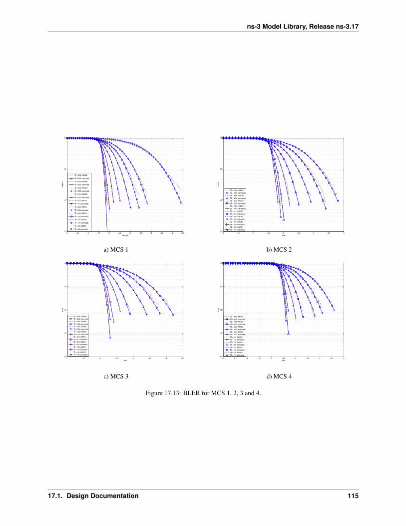
ns-3 Model Library, Release ns-3.17
−9 −8.5 −8 −7.5 −7 −6.5 −6 −5.5 −5 −4.5 −4 −3.510
−3
10−2
10−1
100
SNR [dB]
BL
ER
TB = 6000 (AWGN)
TB = 6000 (estimated)
TB = 4000 (AWGN)
TB = 4000 (estimated)
TB = 2560 (AWGN)
TB = 2560 (estimated)
TB = 1024 (AWGN)
TB = 1024 (estimated)
TB = 512 (AWGN)
TB = 512 (estimated)
TB = 256 (AWGN)
TB = 256 (estimated)
TB = 160 (AWGN)
TB = 160 (estimated)
TB = 104 (AWGN)
TB = 104 (estimated)
TB = 40 (AWGN)
TB = 40 (estimated)
−7 −6.5 −6 −5.5 −5 −4.5 −4 −3.510
−4
10−3
10−2
10−1
100
SNR
BLE
R
TB = 6000 (AWGN)
TB = 6000 (estimated)
TB = 4000 (AWGN)
TB = 4000 (estimated)
TB = 2560 (AWGN)
TB = 2560 (estimated)
TB = 1024 (AWGN)
TB = 1024 (estimated)
TB = 512 (AWGN)
TB = 512 (estimated)
TB = 256 (AWGN)
TB = 256 (estimated)
TB = 160 (AWGN)
TB = 160 (estimated)
TB = 104 (AWGN)
TB = 104 (estimated)
−8 −7.5 −7 −6.5 −6 −5.5 −5 −4.5 −410
−3
10−2
10−1
100
SNR
BLE
R
TB = 6000 (AWGN)
TB = 6000 (estimated)
TB = 4000 (AWGN)
TB = 4000 (estimated)
TB = 2560 (AWGN)
TB = 2560 (estimated)
TB = 1024 (AWGN)
TB = 1024 (estimated)
TB = 512 (AWGN)
TB = 512 (estimated)
TB = 256 (AWGN)
TB = 256 (estimated)
TB = 160 (AWGN)
TB = 160 (estimated)
TB = 104 (AWGN)
TB = 104 (estimated)
−7 −6.5 −6 −5.5 −5 −4.5 −4 −3.5 −3 −2.5 −210
−4
10−3
10−2
10−1
100
SNR
BLE
R
TB = 6000 (AWGN)
TB = 6000 (estimated)
TB = 4000 (AWGN)
TB = 4000 (estimated)
TB = 2560 (AWGN)
TB = 2560 (estimated)
TB = 1024 (AWGN)
TB = 1024 (estimated)
TB = 512 (AWGN)
TB = 512 (estimated)
TB = 256 (AWGN)
TB = 256 (estimated)
TB = 160 (AWGN)
TB = 160 (estimated)
TB = 104 (AWGN)
TB = 104 (estimated)
a) MCS 1 b) MCS 2
d) MCS 4c) MCS 3
Figure 17.13: BLER for MCS 1, 2, 3 and 4.
17.1. Design Documentation 115
ns-3 Model Library, Release ns-3.17
−5 −4.5 −4 −3.5 −3 −2.5 −2 −1.5 −1 −0.510
−3
10−2
10−1
100
SNR
BL
ER
TB = 6000 (AWGN)
TB = 6000 (estimated)
TB = 4000 (AWGN)
TB = 4000 (estimated)
TB = 2560 (AWGN)
TB = 2560 (estimated)
TB = 1024 (AWGN)
TB = 1024 (estimated)
TB = 512 (AWGN)
TB = 512 (estimated)
TB = 256 (AWGN)
TB = 256 (estimated)
TB = 160 (AWGN)
TB = 160 (estimated)
−2 −1.5 −1 −0.5 0 0.5 110
−3
10−2
10−1
100
SNR
BLE
R
TB = 6000 (AWGN)
TB = 6000 (estimated)
TB = 4000 (AWGN)
TB = 4000 (estimated)
TB = 2560 (AWGN)
TB = 2560 (estimated)
TB = 1024 (AWGN)
TB = 1024 (estimated)
TB = 512 (AWGN)
TB = 512 (estimated)
TB = 256 (AWGN)
TB = 256 (estimated)
−5 −4.5 −4 −3.5 −3 −2.5 −210
−3
10−2
10−1
100
SNR
BL
ER
TB = 6000 (AWGN)
TB = 6000 (estimated)
TB = 4000 (AWGN)
TB = 4000 (estimated)
TB = 2560 (AWGN)
TB = 2560 (estimated)
TB = 1024 (AWGN)
TB = 1024 (estimated)
TB = 512 (AWGN)
TB = 512 (estimated)
TB = 256 (AWGN)
TB = 256 (estimated)
−5 −4.5 −4 −3.5 −3 −2.5 −2 −1.5 −1 −0.5 010
−4
10−3
10−2
10−1
100
SNR
BLE
R
TB = 6000 (AWGN)
TB = 6000 (estimated)
TB = 4000 (AWGN)
TB = 4000 (estimated)
TB = 2560 (AWGN)
TB = 2560 (estimated)
TB = 1024 (AWGN)
TB = 1024 (estimated)
TB = 512 (AWGN)
TB = 512 (estimated)
TB = 256 (AWGN)
TB = 256 (estimated)
a) MCS 5 b) MCS 6
d) MCS 8c) MCS 7
Figure 17.14: BLER for MCS 5, 6, 7 and 8.
116 Chapter 17. LTE Module
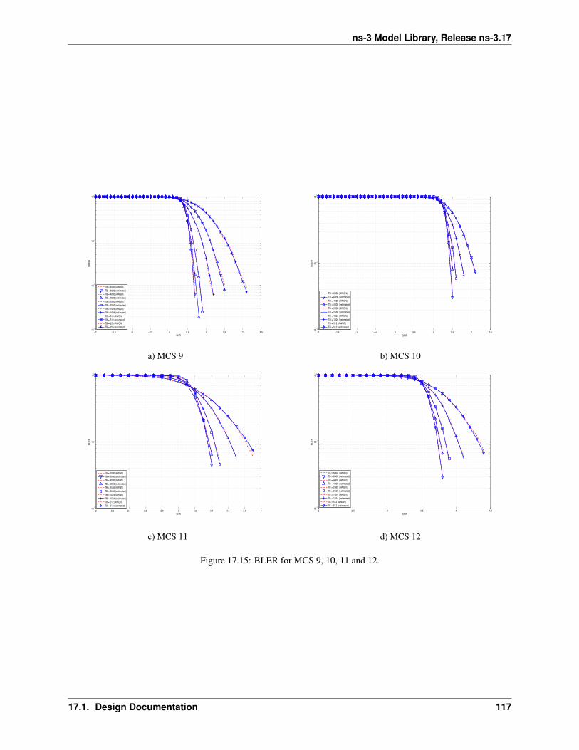
ns-3 Model Library, Release ns-3.17
2 2.2 2.4 2.6 2.8 3 3.2 3.4 3.6 3.8 410
−2
10−1
100
SNR
BLE
R
TB = 6000 (AWGN)
TB = 6000 (estimated)
TB = 4000 (AWGN)
TB = 4000 (estimated)
TB = 2560 (AWGN)
TB = 2560 (estimated)
TB = 1024 (AWGN)
TB = 1024 (estimated)
TB = 512 (AWGN)
TB = 512 (estimated)
−2 −1.5 −1 −0.5 0 0.5 1 1.5 2 2.510
−3
10−2
10−1
100
SNR
BL
ER
TB = 6000 (AWGN)
TB = 6000 (estimated)
TB = 4000 (AWGN)
TB = 4000 (estimated)
TB = 2560 (AWGN)
TB = 2560 (estimated)
TB = 1024 (AWGN)
TB = 1024 (estimated)
TB = 512 (AWGN)
TB = 512 (estimated)
TB = 256 (AWGN)
TB = 256 (estimated)
−2 −1.5 −1 −0.5 0 0.5 1 1.5 2 2.510
−2
10−1
100
SNR
BLE
R
TB = 6000 (AWGN)
TB = 6000 (estimated)
TB = 4000 (AWGN)
TB = 4000 (estimated)
TB = 2560 (AWGN)
TB = 2560 (estimated)
TB = 1024 (AWGN)
TB = 1024 (estimated)
TB = 512 (AWGN)
TB = 512 (estimated)
2 2.5 3 3.5 4 4.510
−2
10−1
100
SNR
BLE
R
TB = 6000 (AWGN)
TB = 6000 (estimated)
TB = 4000 (AWGN)
TB = 4000 (estimated)
TB = 2560 (AWGN)
TB = 2560 (estimated)
TB = 1024 (AWGN)
TB = 1024 (estimated)
TB = 512 (AWGN)
TB = 512 (estimated)
a) MCS 9
d) MCS 12c) MCS 11
b) MCS 10
Figure 17.15: BLER for MCS 9, 10, 11 and 12.
17.1. Design Documentation 117
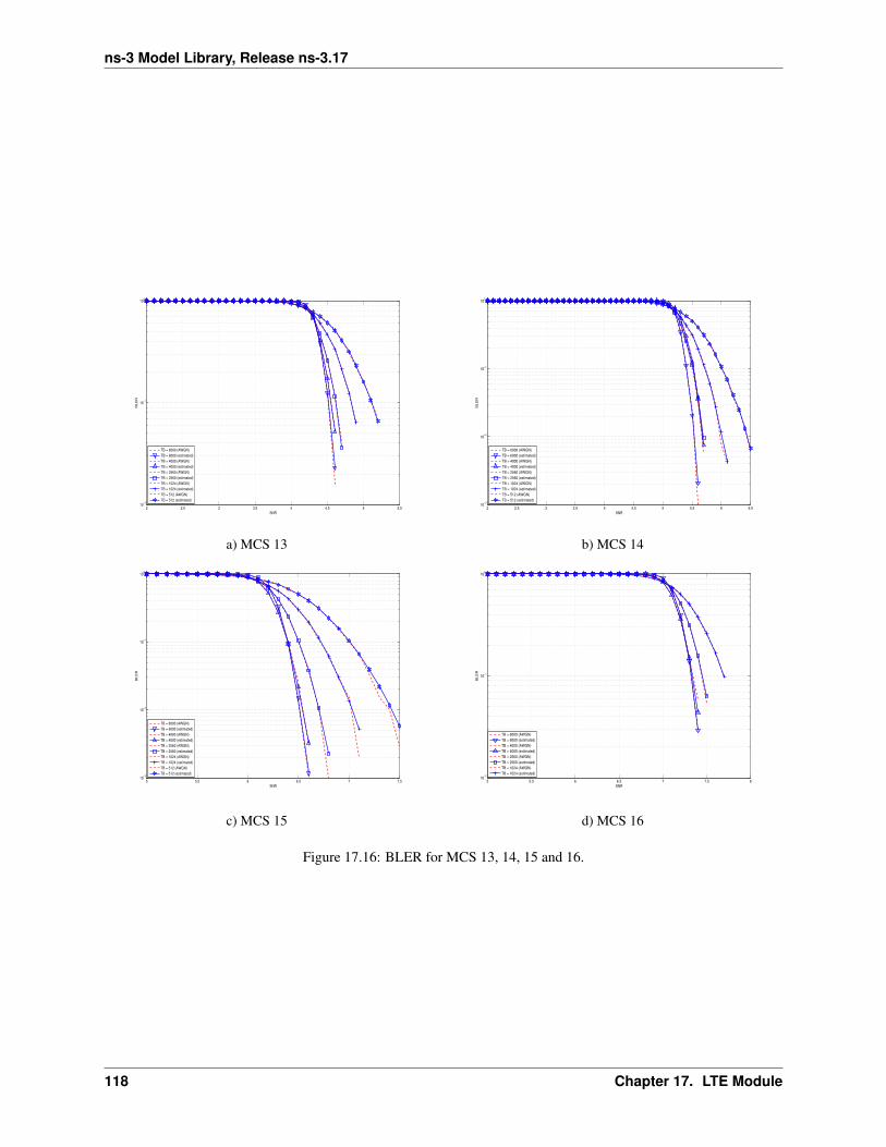
ns-3 Model Library, Release ns-3.17
2 2.5 3 3.5 4 4.5 5 5.510
−2
10−1
100
SNR
BL
ER
TB = 6000 (AWGN)
TB = 6000 (estimated)
TB = 4000 (AWGN)
TB = 4000 (estimated)
TB = 2560 (AWGN)
TB = 2560 (estimated)
TB = 1024 (AWGN)
TB = 1024 (estimated)
TB = 512 (AWGN)
TB = 512 (estimated)
5 5.5 6 6.5 7 7.510
−3
10−2
10−1
100
SNR
BLE
R
TB = 6000 (AWGN)
TB = 6000 (estimated)
TB = 4000 (AWGN)
TB = 4000 (estimated)
TB = 2560 (AWGN)
TB = 2560 (estimated)
TB = 1024 (AWGN)
TB = 1024 (estimated)
TB = 512 (AWGN)
TB = 512 (estimated)
5 5.5 6 6.5 7 7.5 810
−2
10−1
100
SNR
BLE
R
TB = 6000 (AWGN)
TB = 6000 (estimated)
TB = 4000 (AWGN)
TB = 4000 (estimated)
TB = 2560 (AWGN)
TB = 2560 (estimated)
TB = 1024 (AWGN)
TB = 1024 (estimated)
2 2.5 3 3.5 4 4.5 5 5.5 6 6.510
−3
10−2
10−1
100
SNR
BL
ER
TB = 6000 (AWGN)
TB = 6000 (estimated)
TB = 4000 (AWGN)
TB = 4000 (estimated)
TB = 2560 (AWGN)
TB = 2560 (estimated)
TB = 1024 (AWGN)
TB = 1024 (estimated)
TB = 512 (AWGN)
TB = 512 (estimated)
d) MCS 16c) MCS 15
b) MCS 14a) MCS 13
Figure 17.16: BLER for MCS 13, 14, 15 and 16.
118 Chapter 17. LTE Module
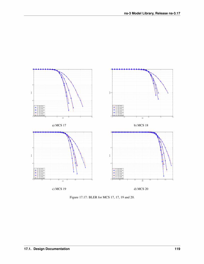
ns-3 Model Library, Release ns-3.17
8 8.5 9 9.5 10 10.510
−2
10−1
100
SNR
BLE
R
TB = 6000 (AWGN)
TB = 6000 (estimated)
TB = 4000 (AWGN)
TB = 4000 (estimated)
TB = 2560 (AWGN)
TB = 2560 (estimated)
TB = 1024 (AWGN)
TB = 1024 (estimated)
8 8.5 9 9.5 10 10.5 11 11.510
−3
10−2
10−1
100
SNR
BLE
R
TB = 6000 (AWGN)
TB = 6000 (estimated)
TB = 4000 (AWGN)
TB = 4000 (estimated)
TB = 2560 (AWGN)
TB = 2560 (estimated)
TB = 1024 (AWGN)
TB = 1024 (estimated)
7 7.5 8 8.5 9 9.510
−3
10−2
10−1
100
SNR
BL
ER
TB = 6000 (AWGN)
TB = 6000 (estimated)
TB = 4000 (AWGN)
TB = 4000 (estimated)
TB = 2560 (AWGN)
TB = 2560 (estimated)
TB = 1024 (AWGN)
TB = 1024 (estimated)
8 8.5 9 9.5 10 10.5 11 11.5 1210
−3
10−2
10−1
100
SNR
BLE
R
TB = 6000 (AWGN)
TB = 6000 (estimated)
TB = 4000 (AWGN)
TB = 4000 (estimated)
TB = 2560 (AWGN)
TB = 2560 (estimated)
TB = 1024 (AWGN)
TB = 1024 (estimated)
d) MCS 20c) MCS 19
a) MCS 17 b) MCS 18
Figure 17.17: BLER for MCS 17, 17, 19 and 20.
17.1. Design Documentation 119
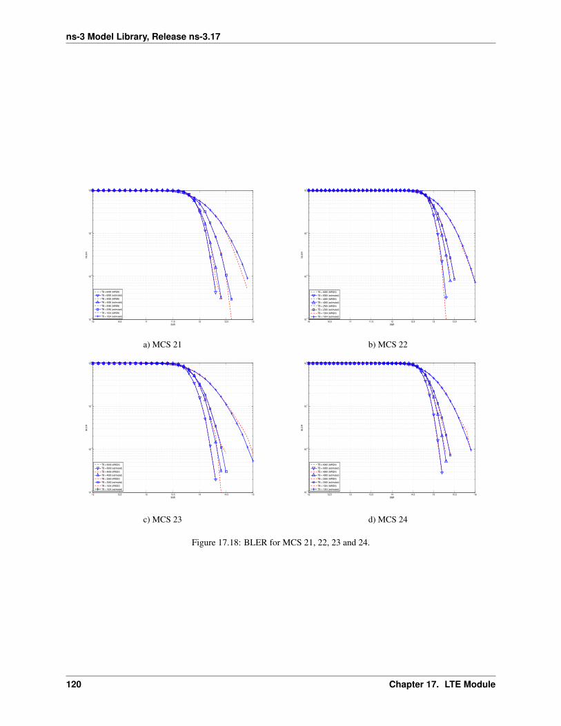
ns-3 Model Library, Release ns-3.17
10 10.5 11 11.5 12 12.5 1310
−3
10−2
10−1
100
SNR
BL
ER
TB = 6000 (AWGN)
TB = 6000 (estimated)
TB = 4000 (AWGN)
TB = 4000 (estimated)
TB = 2560 (AWGN)
TB = 2560 (estimated)
TB = 1024 (AWGN)
TB = 1024 (estimated)
12 12.5 13 13.5 14 14.5 1510
−3
10−2
10−1
100
SNR
BLE
R
TB = 6000 (AWGN)
TB = 6000 (estimated)
TB = 4000 (AWGN)
TB = 4000 (estimated)
TB = 2560 (AWGN)
TB = 2560 (estimated)
TB = 1024 (AWGN)
TB = 1024 (estimated)
12 12.5 13 13.5 14 14.5 15 15.5 1610
−3
10−2
10−1
100
SNR
BLE
R
TB = 6000 (AWGN)
TB = 6000 (estimated)
TB = 4000 (AWGN)
TB = 4000 (estimated)
TB = 2560 (AWGN)
TB = 2560 (estimated)
TB = 1024 (AWGN)
TB = 1024 (estimated)
10 10.5 11 11.5 12 12.5 13 13.5 1410
−3
10−2
10−1
100
SNR
BL
ER
TB = 6000 (AWGN)
TB = 6000 (estimated)
TB = 4000 (AWGN)
TB = 4000 (estimated)
TB = 2560 (AWGN)
TB = 2560 (estimated)
TB = 1024 (AWGN)
TB = 1024 (estimated)
d) MCS 24c) MCS 23
b) MCS 22a) MCS 21
Figure 17.18: BLER for MCS 21, 22, 23 and 24.
120 Chapter 17. LTE Module
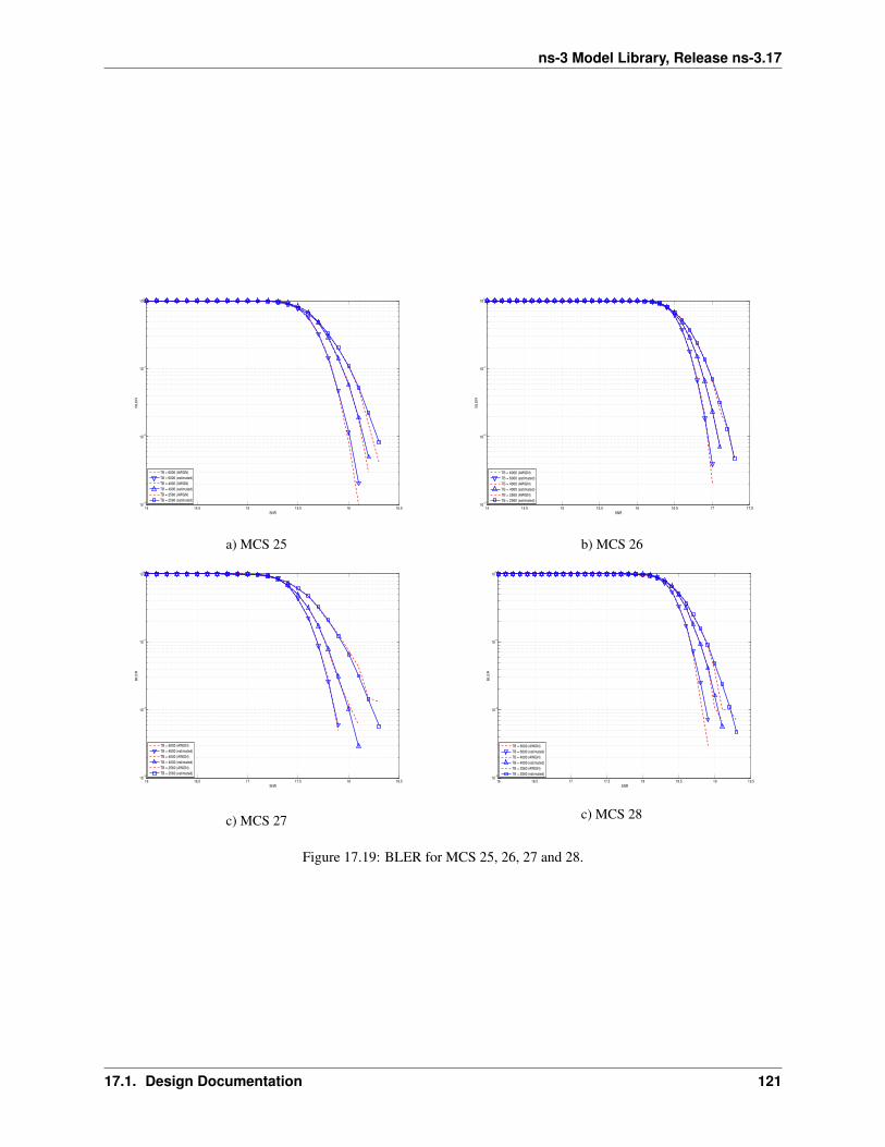
ns-3 Model Library, Release ns-3.17
14 14.5 15 15.5 16 16.5 17 17.510
−3
10−2
10−1
100
SNR
BL
ER
TB = 6000 (AWGN)
TB = 6000 (estimated)
TB = 4000 (AWGN)
TB = 4000 (estimated)
TB = 2560 (AWGN)
TB = 2560 (estimated)
14 14.5 15 15.5 16 16.510
−3
10−2
10−1
100
SNR
BL
ER
TB = 6000 (AWGN)
TB = 6000 (estimated)
TB = 4000 (AWGN)
TB = 4000 (estimated)
TB = 2560 (AWGN)
TB = 2560 (estimated)
16 16.5 17 17.5 18 18.510
−3
10−2
10−1
100
SNR
BLE
R
TB = 6000 (AWGN)
TB = 6000 (estimated)
TB = 4000 (AWGN)
TB = 4000 (estimated)
TB = 2560 (AWGN)
TB = 2560 (estimated)
16 16.5 17 17.5 18 18.5 19 19.510
−3
10−2
10−1
100
SNR
BLE
R
TB = 6000 (AWGN)
TB = 6000 (estimated)
TB = 4000 (AWGN)
TB = 4000 (estimated)
TB = 2560 (AWGN)
TB = 2560 (estimated)
c) MCS 27
b) MCS 26a) MCS 25
c) MCS 28
Figure 17.19: BLER for MCS 25, 26, 27 and 28.
17.1. Design Documentation 121
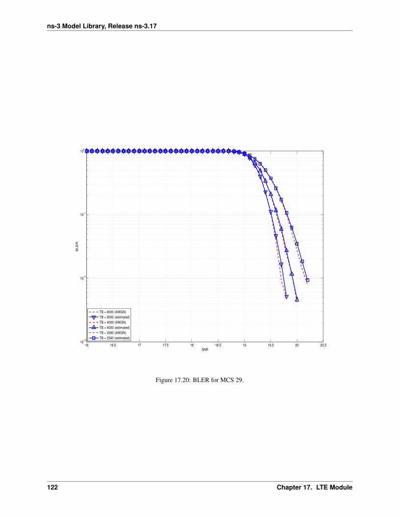
ns-3 Model Library, Release ns-3.17
16 16.5 17 17.5 18 18.5 19 19.5 20 20.510
−3
10−2
10−1
100
SNR
BLE
R
TB = 6000 (AWGN)
TB = 6000 (estimated)
TB = 4000 (AWGN)
TB = 4000 (estimated)
TB = 2560 (AWGN)
TB = 2560 (estimated)
Figure 17.20: BLER for MCS 29.
122 Chapter 17. LTE Module
ns-3 Model Library, Release ns-3.17
Config::SetDefault ("ns3::LteSpectrumPhy::DataErrorModelEnabled", BooleanValue (false));
Control Channels PHY Error Model
The simulator includes the error model for downlink control channels (PCFICH and PDCCH), while in uplink it isassumed and ideal error-free channel. The model is based on the MIESM approach presented before for consideringthe effects of the frequency selective channel since most of the control channels span the whole available bandwidth.
PCFICH + PDCCH Error Model
The model adopted for the error distribution of these channels is based on an evaluation study carried out in the RAN4of 3GPP, where different vendors investigated the demodulation performance of the PCFICH jointly with PDCCH.This is due to the fact that the PCFICH is the channel in charge of communicating to the UEs the actual dimension ofthe PDCCH (which spans between 1 and 3 symbols); therefore the correct decodification of the DCIs depends on thecorrect interpretation of both ones. In 3GPP this problem have been evaluated for improving the cell-edge performance[FujitsuWhitePaper], where the interference among neighboring cells can be relatively high due to signal degradation.A similar problem has been notices in femto-cell scenario and, more in general, in HetNet scenarios the bottleneck hasbeen detected mainly as the PCFICH channel [Bharucha2011], where in case of many eNBs are deployed in the sameservice area, this channel may collide in frequency, making impossible the correct detection of the PDCCH channel,too.
In the simulator, the SINR perceived during the reception has been estimated according to the MIESM model presentedabove in order to evaluate the error distribution of PCFICH and PDCCH. In detail, the SINR samples of all the RBs areincluded in the evaluation of the MI associated to the control frame and, according to this values, the effective SINR(eSINR) is obtained by inverting the MI evaluation process. It has to be noted that, in case of MIMO transmission, bothPCFICH and the PDCCH use always the transmit diversity mode as defined by the standard. According to the eSINRperceived the decodification error probability can be estimated as function of the results presented in [R4-081920].In case an error occur, the DCIs discarded and therefore the UE will be not able to receive the correspondent Tbs,therefore resulting lost.
MIMO Model
The use of multiple antennas both at transmitter and receiver side, known as multiple-input and multiple-output(MIMO), is a problem well studied in literature during the past years. Most of the work concentrate on evaluatinganalytically the gain that the different MIMO schemes might have in term of capacity; however someones provide alsoinformation of the gain in terms of received power [CatreuxMIMO].
According to the considerations above, a model more flexible can be obtained considering the gain that MIMO schemesbring in the system from a statistical point of view. As highlighted before, [CatreuxMIMO] presents the statistical gainof several MIMO solutions respect to the SISO one in case of no correlation between the antennas. In the work thegain is presented as the cumulative distribution function (CDF) of the output SINR for what concern SISO, MIMO-Alamouti, MIMO-MMSE, MIMO-OSIC-MMSE and MIMO-ZF schemes. Elaborating the results, the output SINRdistribution can be approximated with a log-normal one with different mean and variance as function of the schemeconsidered. However, the variances are not so different and they are approximatively equal to the one of the SISOmode already included in the shadowing component of the BuildingsPropagationLossModel, in detail:
• SISO: µ = 13.5 and σ = 20 [dB].
• MIMO-Alamouti: µ = 17.7 and σ = 11.1 [dB].
• MIMO-MMSE: µ = 10.7 and σ = 16.6 [dB].
• MIMO-OSIC-MMSE: µ = 12.6 and σ = 15.5 [dB].
17.1. Design Documentation 123

ns-3 Model Library, Release ns-3.17
• MIMO-ZF: µ = 10.3 and σ = 12.6 [dB].
Therefore the PHY layer implements the MIMO model as the gain perceived by the receiver when using a MIMOscheme respect to the one obtained using SISO one. We note that, these gains referred to a case where there is nocorrelation between the antennas in MIMO scheme; therefore do not model degradation due to paths correlation.
124 Chapter 17. LTE Module
ns-3 Model Library, Release ns-3.17
17.1.6 HARQ
The HARQ scheme implemented is based on a incremental redundancy (IR) solutions combined with multiple stop-and-wait processes for enabling a continuous data flow. In detail, the solution adopted is the soft combining hybridIR Full incremental redundancy (also called IR Type II), which implies that the retransmissions contain only newinformation respect to the previous ones. The resource allocation algorithm of the HARQ has been implemented withinthe respective scheduler classes (i.e., RrFfMacScheduler and PfFfMacScheduler, refer to their correspondentsections for more info), while the decodification part of the HARQ has been implemented in the LteSpectrumPhyand LteHarqPhy classes which will be detailed in this section.
According to the standard, the UL retransmissions are synchronous and therefore are allocated 7 ms after the originaltransmission. On the other hand, for the DL, they are asynchronous and therefore can be allocated in a more flexibleway starting from 7 ms and it is a matter of the specific scheduler implementation. The HARQ processes behavior isdepicted in Figure:ref:fig-harq-processes-scheme.
At the MAC layer, the HARQ entity residing in the scheduler is in charge of controlling the 8 HARQ processesfor generating new packets and managing the retransmissions both for the DL and the UL. The scheduler collectsthe HARQ feedback from eNB and UE PHY layers (respectively for UL and DL connection) by means of the FFAPI primitives SchedUlTriggerReq and SchedUlTriggerReq. According to the HARQ feedback and theRLC buffers status, the scheduler generates a set of DCIs including both retransmissions of HARQ blocks receivederroneous and new transmissions, in general, giving priority to the former. On this matter, the scheduler has to take intoconsideration one constraint when allocating the resource for HARQ retransmissions, it must use the same modulationorder of the first transmission attempt (i.e., QPSK for MCS ∈ [0..9], 16QAM for MCS ∈ [10..16] and 64QAM forMCS ∈ [17..28]). This restriction comes from the specification of the rate matcher in the 3GPP standard [TS36212],where the algorithm fixes the modulation order for generating the different blocks of the redundancy versions.
The PHY Error Model model (i.e., the LteMiErrorModel class already presented before) has been extended forconsidering IR HARQ according to [wimaxEmd], where the parameters for the AWGN curves mapping for MIESMmapping in case of retransmissions are given by:
Reff =Xq∑i=1
Ci
MIeff =
q∑i=1
CiMi
q∑i=1
Ci
where X is the number of original information bits, Ci are number of coded bits, Mi are the mutual informationsper HARQ block received on the total number of q retransmissions. Therefore, in order to be able to return the errorprobability with the error model implemented in the simulator evaluates the Reff and the MIIeff and return thevalue of error probability of the ECR of the same modulation with closest lower rate respect to the Reff . In orderto consider the effect of HARQ retransmissions a new sets of curves have been integrated respect to the standard oneused for the original MCS. The new curves are intended for covering the cases when the most conservative MCS of amodulation is used which implies the generation of Reff lower respect to the one of standard MCSs. On this matterthe curves for 1, 2 and 3 retransmissions have been evaluated for 10 and 17. For MCS 0 we considered only the firstretransmission since the produced code rate is already very conservative (i.e., 0.04) and returns an error rate enoughrobust for the reception (i.e., the downturn of the BLER is centered around -18 dB). It is to be noted that, the size offirst TB transmission has been assumed as containing all the information bits to be coded; therefore X is equal to thesize of the first TB sent of a an HARQ process. The model assumes that the eventual presence of parity bits in thecodewords is already considered in the link level curves. This implies that as soon as the minimum Reff is reachedthe model is not including the gain due to the transmission of further parity bits.
The part of HARQ devoted to manage the decodification of the HARQ blocks has been implemented in theLteHarqPhy and LteSpectrumPhy classes. The former is in charge of maintaining the HARQ informationfor each active process . The latter interacts with LteMiErrorModel class for evaluating the correctness of the
17.1. Design Documentation 125
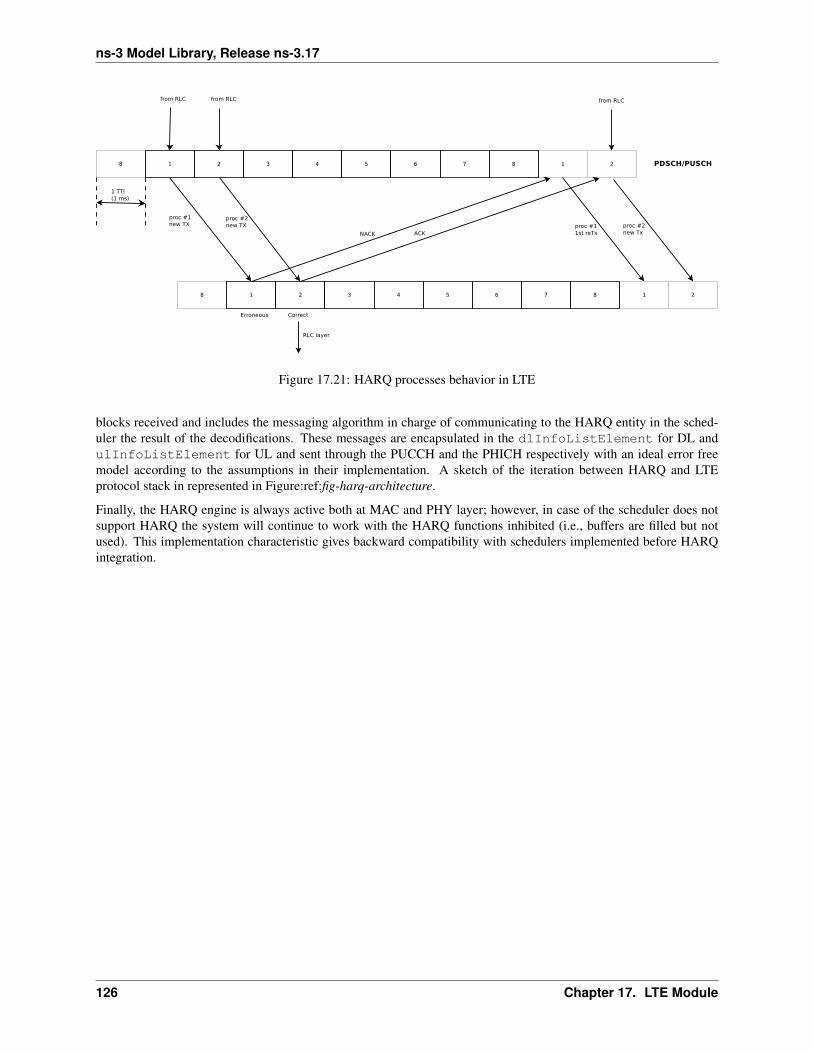
ns-3 Model Library, Release ns-3.17
Figure 17.21: HARQ processes behavior in LTE
blocks received and includes the messaging algorithm in charge of communicating to the HARQ entity in the sched-uler the result of the decodifications. These messages are encapsulated in the dlInfoListElement for DL andulInfoListElement for UL and sent through the PUCCH and the PHICH respectively with an ideal error freemodel according to the assumptions in their implementation. A sketch of the iteration between HARQ and LTEprotocol stack in represented in Figure:ref:fig-harq-architecture.
Finally, the HARQ engine is always active both at MAC and PHY layer; however, in case of the scheduler does notsupport HARQ the system will continue to work with the HARQ functions inhibited (i.e., buffers are filled but notused). This implementation characteristic gives backward compatibility with schedulers implemented before HARQintegration.
126 Chapter 17. LTE Module
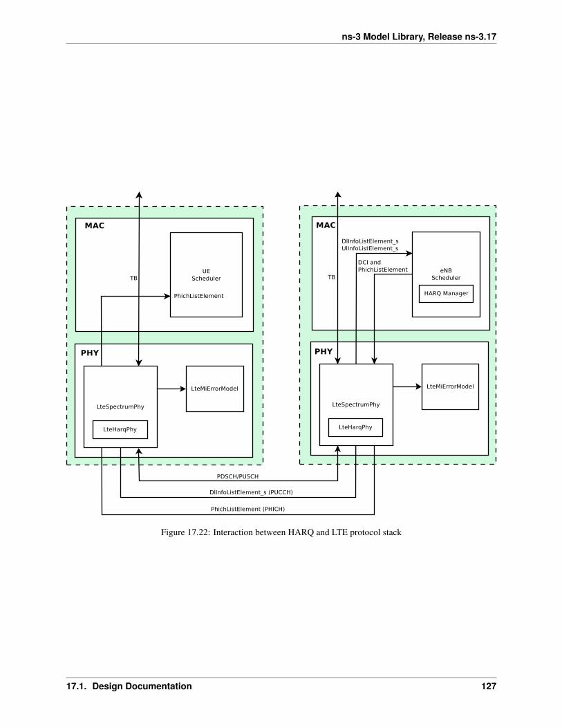
ns-3 Model Library, Release ns-3.17
Figure 17.22: Interaction between HARQ and LTE protocol stack
17.1. Design Documentation 127
ns-3 Model Library, Release ns-3.17
17.1.7 MAC
Resource Allocation Model
We now briefly describe how resource allocation is handled in LTE, clarifying how it is modeled in the simulator. Thescheduler is in charge of generating specific structures calles Data Control Indication (DCI) which are then transmittedby the PHY of the eNB to the connected UEs, in order to inform them of the resource allocation on a per subframebasis. In doing this in the downlink direction, the scheduler has to fill some specific fields of the DCI structure withall the information, such as: the Modulation and Coding Scheme (MCS) to be used, the MAC Transport Block (TB)size, and the allocation bitmap which identifies which RBs will contain the data transmitted by the eNB to each user.
For the mapping of resources to physical RBs, we adopt a localized mapping approach (see [Sesia2009], Section9.2.2.1); hence in a given subframe each RB is always allocated to the same user in both slots. The allocation bitmapcan be coded in different formats; in this implementation, we considered the Allocation Type 0 defined in [TS36213],according to which the RBs are grouped in Resource Block Groups (RBG) of different size determined as a functionof the Transmission Bandwidth Configuration in use.
For certain bandwidth values not all the RBs are usable, since the group size is not a common divisor of the group.This is for instance the case when the bandwidth is equal to 25 RBs, which results in a RBG size of 2 RBs, andtherefore 1 RB will result not addressable. In uplink the format of the DCIs is different, since only adjacent RBs canbe used because of the SC-FDMA modulation. As a consequence, all RBs can be allocated by the eNB regardless ofthe bandwidth configuration.
Adaptive Modulation and Coding
The simulator provides two Adaptive Modulation and Coding (AMC) models: one based on the GSoC model[Piro2011] and one based on the physical error model (described in the following sections).
The former model is a modified version of the model described in [Piro2011], which in turn is inspired from [Seo2004].Our version is described in the following. Let i denote the generic user, and let γi be its SINR. We get the spectralefficiency ηi of user i using the following equations:
BER = 0.00005
Γ =− ln (5 ∗ BER)
1.5
ηi = log2
(1 +
γiΓ
)The procedure described in [R1-081483] is used to get the corresponding MCS scheme. The spectral efficiency isquantized based on the channel quality indicator (CQI), rounding to the lowest value, and is mapped to the corre-sponding MCS scheme.
Finally, we note that there are some discrepancies between the MCS index in [R1-081483] and that indicated by thestandard: [TS36213] Table 7.1.7.1-1 says that the MCS index goes from 0 to 31, and 0 appears to be a valid MCSscheme (TB size is not 0) but in [R1-081483] the first useful MCS index is 1. Hence to get the value as intended bythe standard we need to subtract 1 from the index reported in [R1-081483].
The alternative model is based on the physical error model developed for this simulator and explained in the followingsubsections. This scheme is able to adapt the MCS selection to the actual PHY layer performance according tothe specific CQI report. According to their definition, a CQI index is assigned when a single PDSCH TB with themodulation coding scheme and code rate correspondent to that CQI index in table 7.2.3-1 of [TS36213] can be receivedwith an error probability less than 0.1. In case of wideband CQIs, the reference TB includes all the RBGs available inorder to have a reference based on the whole available resources; while, for subband CQIs, the reference TB is sizedas the RBGs.
128 Chapter 17. LTE Module
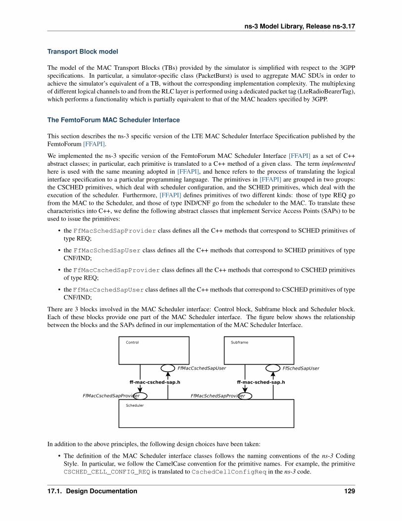
ns-3 Model Library, Release ns-3.17
Transport Block model
The model of the MAC Transport Blocks (TBs) provided by the simulator is simplified with respect to the 3GPPspecifications. In particular, a simulator-specific class (PacketBurst) is used to aggregate MAC SDUs in order toachieve the simulator’s equivalent of a TB, without the corresponding implementation complexity. The multiplexingof different logical channels to and from the RLC layer is performed using a dedicated packet tag (LteRadioBearerTag),which performs a functionality which is partially equivalent to that of the MAC headers specified by 3GPP.
The FemtoForum MAC Scheduler Interface
This section describes the ns-3 specific version of the LTE MAC Scheduler Interface Specification published by theFemtoForum [FFAPI].
We implemented the ns-3 specific version of the FemtoForum MAC Scheduler Interface [FFAPI] as a set of C++abstract classes; in particular, each primitive is translated to a C++ method of a given class. The term implementedhere is used with the same meaning adopted in [FFAPI], and hence refers to the process of translating the logicalinterface specification to a particular programming language. The primitives in [FFAPI] are grouped in two groups:the CSCHED primitives, which deal with scheduler configuration, and the SCHED primitives, which deal with theexecution of the scheduler. Furthermore, [FFAPI] defines primitives of two different kinds: those of type REQ gofrom the MAC to the Scheduler, and those of type IND/CNF go from the scheduler to the MAC. To translate thesecharacteristics into C++, we define the following abstract classes that implement Service Access Points (SAPs) to beused to issue the primitives:
• the FfMacSchedSapProvider class defines all the C++ methods that correspond to SCHED primitives oftype REQ;
• the FfMacSchedSapUser class defines all the C++ methods that correspond to SCHED primitives of typeCNF/IND;
• the FfMacCschedSapProvider class defines all the C++ methods that correspond to CSCHED primitivesof type REQ;
• the FfMacCschedSapUser class defines all the C++ methods that correspond to CSCHED primitives of typeCNF/IND;
There are 3 blocks involved in the MAC Scheduler interface: Control block, Subframe block and Scheduler block.Each of these blocks provide one part of the MAC Scheduler interface. The figure below shows the relationshipbetween the blocks and the SAPs defined in our implementation of the MAC Scheduler Interface.
In addition to the above principles, the following design choices have been taken:
• The definition of the MAC Scheduler interface classes follows the naming conventions of the ns-3 CodingStyle. In particular, we follow the CamelCase convention for the primitive names. For example, the primitiveCSCHED_CELL_CONFIG_REQ is translated to CschedCellConfigReq in the ns-3 code.
17.1. Design Documentation 129
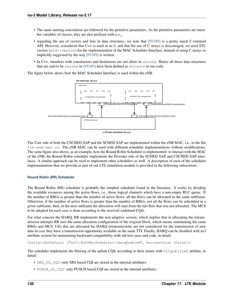
ns-3 Model Library, Release ns-3.17
• The same naming conventions are followed for the primitive parameters. As the primitive parameters are mem-ber variables of classes, they are also prefixed with a m_.
• regarding the use of vectors and lists in data structures, we note that [FFAPI] is a pretty much C-orientedAPI. However, considered that C++ is used in ns-3, and that the use of C arrays is discouraged, we used STLvectors (std::vector) for the implementation of the MAC Scheduler Interface, instead of using C arrays asimplicitly suggested by the way [FFAPI] is written.
• In C++, members with constructors and destructors are not allow in unions. Hence all those data structuresthat are said to be unions in [FFAPI] have been defined as structs in our code.
The figure below shows how the MAC Scheduler Interface is used within the eNB.
The User side of both the CSCHED SAP and the SCHED SAP are implemented within the eNB MAC, i.e., in the filelte-enb-mac.cc. The eNB MAC can be used with different scheduler implementations without modifications.The same figure also shows, as an example, how the Round Robin Scheduler is implemented: to interact with the MACof the eNB, the Round Robin scheduler implements the Provider side of the SCHED SAP and CSCHED SAP inter-faces. A similar approach can be used to implement other schedulers as well. A description of each of the schedulerimplementations that we provide as part of our LTE simulation module is provided in the following subsections.
Round Robin (RR) Scheduler
The Round Robin (RR) scheduler is probably the simplest scheduler found in the literature. It works by dividingthe available resources among the active flows, i.e., those logical channels which have a non-empty RLC queue. Ifthe number of RBGs is greater than the number of active flows, all the flows can be allocated in the same subframe.Otherwise, if the number of active flows is greater than the number of RBGs, not all the flows can be scheduled in agiven subframe; then, in the next subframe the allocation will start from the last flow that was not allocated. The MCSto be adopted for each user is done according to the received wideband CQIs.
For what concern the HARQ, RR implements the non adaptive version, which implies that in allocating the retrans-mission attempts RR uses the same allocation configuration of the original block, which means maintaining the sameRBGs and MCS. UEs that are allocated for HARQ retransmissions are not considered for the transmission of newdata in case they have a transmission opportunity available in the same TTI. Finally, HARQ can be disabled with ns3attribute system for maintaining backward compatibility with old test cases and code, in detail:
Config::SetDefault ("ns3::RrFfMacScheduler::HarqEnabled", BooleanValue (false));
The scheduler implements the filtering of the uplink CQIs according to their nature with UlCqiFilter attibute, indetail:
• SRS_UL_CQI: only SRS based CQI are stored in the internal attributes.
• PUSCH_UL_CQI: only PUSCH based CQI are stored in the internal attributes.
130 Chapter 17. LTE Module
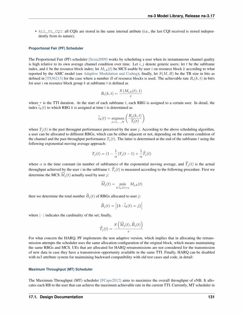
ns-3 Model Library, Release ns-3.17
• ALL_UL_CQI: all CQIs are stored in the same internal attibute (i.e., the last CQI received is stored indepen-dently from its nature).
Proportional Fair (PF) Scheduler
The Proportional Fair (PF) scheduler [Sesia2009] works by scheduling a user when its instantaneous channel qualityis high relative to its own average channel condition over time. Let i, j denote generic users; let t be the subframeindex, and k be the resource block index; let Mi,k(t) be MCS usable by user i on resource block k according to whatreported by the AMC model (see Adaptive Modulation and Coding); finally, let S(M,B) be the TB size in bits asdefined in [TS36213] for the case where a number B of resource blocks is used. The achievable rate Ri(k, t) in bit/sfor user i on resource block group k at subframe t is defined as
Ri(k, t) =S (Mi,k(t), 1)
τ
where τ is the TTI duration. At the start of each subframe t, each RBG is assigned to a certain user. In detail, theindex ik(t) to which RBG k is assigned at time t is determined as
ik(t) = argmaxj=1,...,N
(Rj(k, t)Tj(t)
)where Tj(t) is the past througput performance perceived by the user j. According to the above scheduling algorithm,a user can be allocated to different RBGs, which can be either adjacent or not, depending on the current condition ofthe channel and the past throughput performance Tj(t). The latter is determined at the end of the subframe t using thefollowing exponential moving average approach:
Tj(t) = (1− 1α
)Tj(t− 1) +1αTj(t)
where α is the time constant (in number of subframes) of the exponential moving average, and Tj(t) is the actualthroughput achieved by the user i in the subframe t. Tj(t) is measured according to the following procedure. First wedetermine the MCS Mj(t) actually used by user j:
Mj(t) = mink:bik(t)=j
Mj,k(t)
then we determine the total number Bj(t) of RBGs allocated to user j:
Bj(t) =∣∣∣{k : ik(t) = j}
∣∣∣where | · | indicates the cardinality of the set; finally,
Tj(t) =S(Mj(t), Bj(t)
)τ
For what concern the HARQ, PF implements the non adaptive version, which implies that in allocating the retrans-mission attempts the scheduler uses the same allocation configuration of the original block, which means maintainingthe same RBGs and MCS. UEs that are allocated for HARQ retransmissions are not considered for the transmissionof new data in case they have a transmission opportunity available in the same TTI. Finally, HARQ can be disabledwith ns3 attribute system for maintaining backward compatibility with old test cases and code, in detail:
Maximum Throughput (MT) Scheduler
The Maximum Throughput (MT) scheduler [FCapo2012] aims to maximize the overall throughput of eNB. It allo-cates each RB to the user that can achieve the maximum achievable rate in the current TTI. Currently, MT scheduler in
17.1. Design Documentation 131
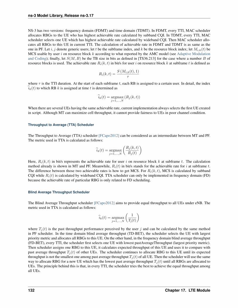
ns-3 Model Library, Release ns-3.17
NS-3 has two versions: frequency domain (FDMT) and time domain (TDMT). In FDMT, every TTI, MAC schedulerallocates RBGs to the UE who has highest achievable rate calculated by subband CQI. In TDMT, every TTI, MACscheduler selects one UE which has highest achievable rate calculated by wideband CQI. Then MAC scheduler allo-cates all RBGs to this UE in current TTI. The calculation of achievable rate in FDMT and TDMT is as same as theone in PF. Let i, j denote generic users; let t be the subframe index, and k be the resource block index; let Mi,k(t) beMCS usable by user i on resource block k according to what reported by the AMC model (see Adaptive Modulationand Coding); finally, let S(M,B) be the TB size in bits as defined in [TS36.213] for the case where a number B ofresource blocks is used. The achievable rate Ri(k, t) in bit/s for user i on resource block k at subframe t is defined as
Ri(k, t) =S (Mi,k(t), 1)
τ
where τ is the TTI duration. At the start of each subframe t, each RB is assigned to a certain user. In detail, the indexik(t) to which RB k is assigned at time t is determined as
ik(t) = argmaxj=1,...,N
(Rj(k, t))
When there are several UEs having the same achievable rate, current implementation always selects the first UE createdin script. Although MT can maximize cell throughput, it cannot provide fairness to UEs in poor channel condition.
Throughput to Average (TTA) Scheduler
The Throughput to Average (TTA) scheduler [FCapo2012] can be considered as an intermediate between MT and PF.The metric used in TTA is calculated as follows:
ik(t) = argmaxj=1,...,N
(Rj(k, t)Rj(t)
)Here, Ri(k, t) in bit/s represents the achievable rate for user i on resource block k at subframe t. The calculationmethod already is shown in MT and PF. Meanwhile, Ri(t) in bit/s stands for the achievable rate for i at subframe t.The difference between those two achievable rates is how to get MCS. For Ri(k, t), MCS is calculated by subbandCQI while Ri(t) is calculated by wideband CQI. TTA scheduler can only be implemented in frequency domain (FD)because the achievable rate of particular RBG is only related to FD scheduling.
Blind Average Throughput Scheduler
The Blind Average Throughput scheduler [FCapo2012] aims to provide equal throughput to all UEs under eNB. Themetric used in TTA is calculated as follows:
ik(t) = argmaxj=1,...,N
(1
Tj(t)
)where Tj(t) is the past throughput performance perceived by the user j and can be calculated by the same methodin PF scheduler. In the time domain blind average throughput (TD-BET), the scheduler selects the UE with largestpriority metric and allocates all RBGs to this UE. On the other hand, in the frequency domain blind average throughput(FD-BET), every TTI, the scheduler first selects one UE with lowest pastAverageThroughput (largest priority metric).Then scheduler assigns one RBG to this UE, it calculates expected throughput of this UE and uses it to compare withpast average throughput Tj(t) of other UEs. The scheduler continues to allocate RBG to this UE until its expectedthroughput is not the smallest one among past average throughput Tj(t) of all UE. Then the scheduler will use the sameway to allocate RBG for a new UE which has the lowest past average throughput Tj(t) until all RBGs are allocated toUEs. The principle behind this is that, in every TTI, the scheduler tries the best to achieve the equal throughput amongall UEs.
132 Chapter 17. LTE Module
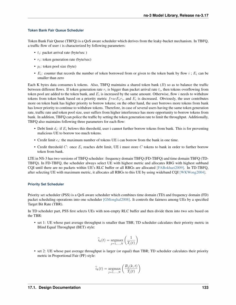
ns-3 Model Library, Release ns-3.17
Token Bank Fair Queue Scheduler
Token Bank Fair Queue (TBFQ) is a QoS aware scheduler which derives from the leaky-bucket mechanism. In TBFQ,a traffic flow of user i is characterized by following parameters:
• ti: packet arrival rate (byte/sec )
• ri: token generation rate (byte/sec)
• pi: token pool size (byte)
• Ei: counter that records the number of token borrowed from or given to the token bank by flow i ; Ei can besmaller than zero
Each K bytes data consumes k tokens. Also, TBFQ maintains a shared token bank (B) so as to balance the trafficbetween different flows. If token generation rate ri is bigger than packet arrival rate ti, then tokens overflowing fromtoken pool are added to the token bank, and Ei is increased by the same amount. Otherwise, flow i needs to withdrawtokens from token bank based on a priority metric fracEiri, and Ei is decreased. Obviously, the user contributesmore on token bank has higher priority to borrow tokens; on the other hand, the user borrows more tokens from bankhas lower priority to continue to withdraw tokens. Therefore, in case of several users having the same token generationrate, traffic rate and token pool size, user suffers from higher interference has more opportunity to borrow tokens frombank. In addition, TBFQ can police the traffic by setting the token generation rate to limit the throughput. Additionally,TBFQ also maintains following three parameters for each flow:
• Debt limit di: if Ei belows this threshold, user i cannot further borrow tokens from bank. This is for preventingmalicious UE to borrow too much tokens.
• Credit limit ci: the maximum number of tokens UE i can borrow from the bank in one time.
• Credit threshold C: once Ei reaches debt limit, UE i must store C tokens to bank in order to further borrowtoken from bank.
LTE in NS-3 has two versions of TBFQ scheduler: frequency domain TBFQ (FD-TBFQ) and time domain TBFQ (TD-TBFQ). In FD-TBFQ, the scheduler always select UE with highest metric and allocates RBG with highest subbandCQI until there are no packets within UE’s RLC buffer or all RBGs are allocated [FABokhari2009]. In TD-TBFQ,after selecting UE with maximum metric, it allocates all RBGs to this UE by using wideband CQI [WKWong2004].
Priority Set Scheduler
Priority set scheduler (PSS) is a QoS aware scheduler which combines time domain (TD) and frequency domain (FD)packet scheduling operations into one scheduler [GMonghal2008]. It controls the fairness among UEs by a specifiedTarget Bit Rate (TBR).
In TD scheduler part, PSS first selects UEs with non-empty RLC buffer and then divide them into two sets based onthe TBR:
• set 1: UE whose past average throughput is smaller than TBR; TD scheduler calculates their priority metric inBlind Equal Throughput (BET) style:
ik(t) = argmaxj=1,...,N
(1
Tj(t)
)• set 2: UE whose past average throughput is larger (or equal) than TBR; TD scheduler calculates their priority
metric in Proportional Fair (PF) style:
ik(t) = argmaxj=1,...,N
(Rj(k, t)Tj(t)
)
17.1. Design Documentation 133
ns-3 Model Library, Release ns-3.17
UEs belonged to set 1 have higher priority than ones in set 2. Then PSS will select Nmux UEs with highest metric intwo sets and forward those UE to FD scheduler. In PSS, FD scheduler allocates RBG k to UE n that maximums thechosen metric. Two PF schedulers are used in PF scheduler:
• Proportional Fair scheduled (PFsch)
Mschk(t) = argmaxj=1,...,N
(Rj(k, t)Tschj(t)
)• Carrier over Interference to Average (CoIta)
Mcoik(t) = argmaxj=1,...,N
(CoI[j, k]∑NRBG
k=0 CoI[j, k]
)
where Tschj(t) is similar past throughput performance perceived by the user j, with the difference that it is updatedonly when the i-th user is actually served. CoI[j, k] is an estimation of the SINR on the RBG k of UE j. Both PFschand CoIta is for decoupling FD metric from TD scheduler. In addition, PSS FD scheduler also provide a weight metricW[n] for helping controlling fairness in case of low number of UEs.
W [n] = max(1,TBR
Tj(t))
where Tj(t) is the past throughput performance perceived by the user j . Therefore, on RBG k, the FD schedulerselects the UE j that maximizes the product of the frequency domain metric (Msch, MCoI) by weight W [n]. Thisstrategy will guarantee the throughput of lower quality UE tend towards the TBR.
Config::SetDefault (“ns3::PfFfMacScheduler::HarqEnabled”, BooleanValue (false));
The scheduler implements the filtering of the uplink CQIs according to their nature with UlCqiFilter attibute, indetail:
• SRS_UL_CQI: only SRS based CQI are stored in the internal attributes.
• PUSCH_UL_CQI: only PUSCH based CQI are stored in the internal attributes.
• ALL_UL_CQI: all CQIs are stored in the same internal attibute (i.e., the last CQI received is stored indepen-dently from its nature).
Random Access
The LTE model includes a model of the Random Access procedure based on some simplifying assumptions, whichare detailed in the following for each of the messages and signals described in the specs [TS36321].
• Random Access (RA) preamble: in real LTE systems this corresponds to a Zadoff-Chu (ZC) sequence usingone of several formats available and sent in the PRACH slots which could in principle overlap with PUSCH. TheRA preamble is modeled using the LteControlMessage class, i.e., as an ideal message that does not consumeany radio resources. The collision of preamble transmission by multiple UEs in the same cell are modeled usinga protocol interference model, i.e., whenever two or more identical preambles are transmitted in same cell at thesame TTI, no one of these identical preambles will be received by the eNB. Other than this collision model, noerror model is associated with the reception of a RA preamble.
• Random Access Response (RAR): in real LTE systems, this is a special MAC PDU sent on the DL-SCH.Since MAC control elements are not accurately modeled in the simulator (only RLC and above PDUs are), theRAR is modeled as an LteControlMessage that does not consume any radio resources. Still, during the RAprocedure, the LteEnbMac will request to the scheduler the allocation of resources for the RAR using the FFMAC Scheduler primitive SCHED_DL_RACH_INFO_REQ. Hence, an enhanced scheduler implementation(not available at the moment) could allocate radio resources for the RAR, thus modeling the consumption ofRadio Resources for the transmission of the RAR.
134 Chapter 17. LTE Module
ns-3 Model Library, Release ns-3.17
• Message 3: in real LTE systems, this is an RLC TM SDU sent over resources specified in the UL Grant in theRAR. In the simulator, this is modeled as a real RLC TM RLC PDU whose UL resources are allocated by thescheduler upon call to SCHED_DL_RACH_INFO_REQ.
• Contention Resolution (CR): in real LTE system, the CR phase is needed to address the case where two ormore UE sent the same RA preamble in the same TTI, and the eNB was able to detect this preamble in spite ofthe collision. Since this event does not occur due to the protocol interference model used for the reception ofRA preambles, the CR phase is not modeled in the simulator, i.e., the CR MAC CE is never sent by the eNB andthe UEs consider the RA to be successful upon reception of the RAR. As a consequence, the radio resourcesconsumed for the transmission of the CR MAC CE are not modeled.
Figure Sequence diagram of the Contention-based MAC Random Access procedure and Sequence diagram of the Non-contention-based MAC Random Access procedure shows the sequence diagrams of respectively the contention-basedand non-contention-based MAC random access procedure, highlighting the interactions between the MAC and theother entities.
17.1. Design Documentation 135
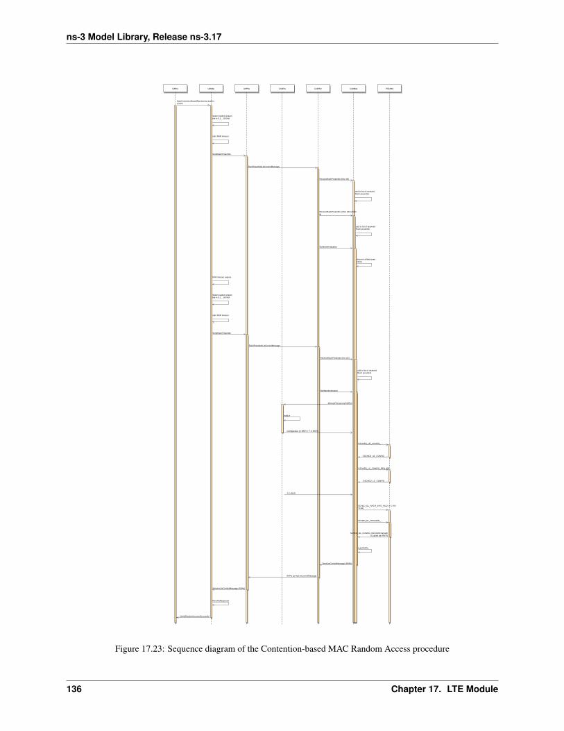
ns-3 Model Library, Release ns-3.17
UeRrc UeMac UePhy EnbRrc EnbPhy EnbMac FfSched
StartContentionBasedRandomAccessProcedure
Select random preamble in 0,1,...,63-Ncf
start RAR timeout
SendRachPreamble
RachPreambleLteControlMessage
ReceiveRachPreamble (this UE)
add to list of receivedRach preamble
ReceiveRachPreamble (other UE colliding)
add to list of receivedRach preamble
SubframeIndication
discard collided preambles
RAR timeout expires
Select random preamble in 0,1,...,63-Ncf
start RAR timeout
SendRachPreamble
RachPreambleLteControlMessage
ReceiveRachPreamble (this UE)
add to list of receivedRach preamble
SubframeIndication
AllocateTemporaryCellRnti
AddUe
ConfigureUe (C-RNTI = T-C-RNTI)
CSCHED_UE_CONFIG_ ...
CSCHED_UE_CONFIG_ ...
CSCHED_LC_CONFIG_REQ (SR ...
CSCHED_LC_CONFIG_ ...
T-C-RNTI
SCHED_DL_RACH_INFO_REQ (T-C-RNTI list)
SCHED_DL_TRIGGER_ ...
SCHED_DL_CONFIG_IND (RAR list withUL grant per RNTI)
build RARs
SendLteControlMessage (RARs)
RARs as RarLteControlMessage
ReceiveLteControlMessage (RARs)
RecvRaResponse
NotifyRandomAccessSuccessful
Figure 17.23: Sequence diagram of the Contention-based MAC Random Access procedure
136 Chapter 17. LTE Module
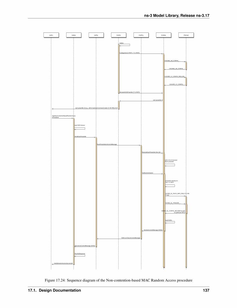
ns-3 Model Library, Release ns-3.17
UeRrc UeMac UePhy EnbRrc EnbPhy EnbMac FfSched
AddUe
ConfigureUe (C-RNTI = T-C-RNTI)
CSCHED_UE_CONFIG_ ...
CSCHED_UE_CONFIG_ ...
CSCHED_LC_CONFIG_REQ (SR ...
CSCHED_LC_CONFIG_ ...
AllocateNcRaPreamble (T-C-RNTI)
rach preamble id
rach preamble id (e.g., within handoverCommand inside X2 HO REQ ACK
StartNonContentionBasedRandomAccessProcedure
start RAR timeout
SendRachPreamble
RachPreambleLteControlMessage
ReceiveRachPreamble (this UE)
add to list of receivedRach preamble
SubframeIndication
preamble matches known T-C-RNTI
SCHED_DL_RACH_INFO_REQ (T-C-RNTI list)
SCHED_DL_TRIGGER_ ...
SCHED_DL_CONFIG_IND (RAR list withUL grant per RNTI)
build RARs
SendLteControlMessage (RARs)
RARs as RarLteControlMessage
ReceiveLteControlMessage (RARs)
RecvRaResponse
NotifyRandomAccessSuccessful
Figure 17.24: Sequence diagram of the Non-contention-based MAC Random Access procedure
17.1. Design Documentation 137
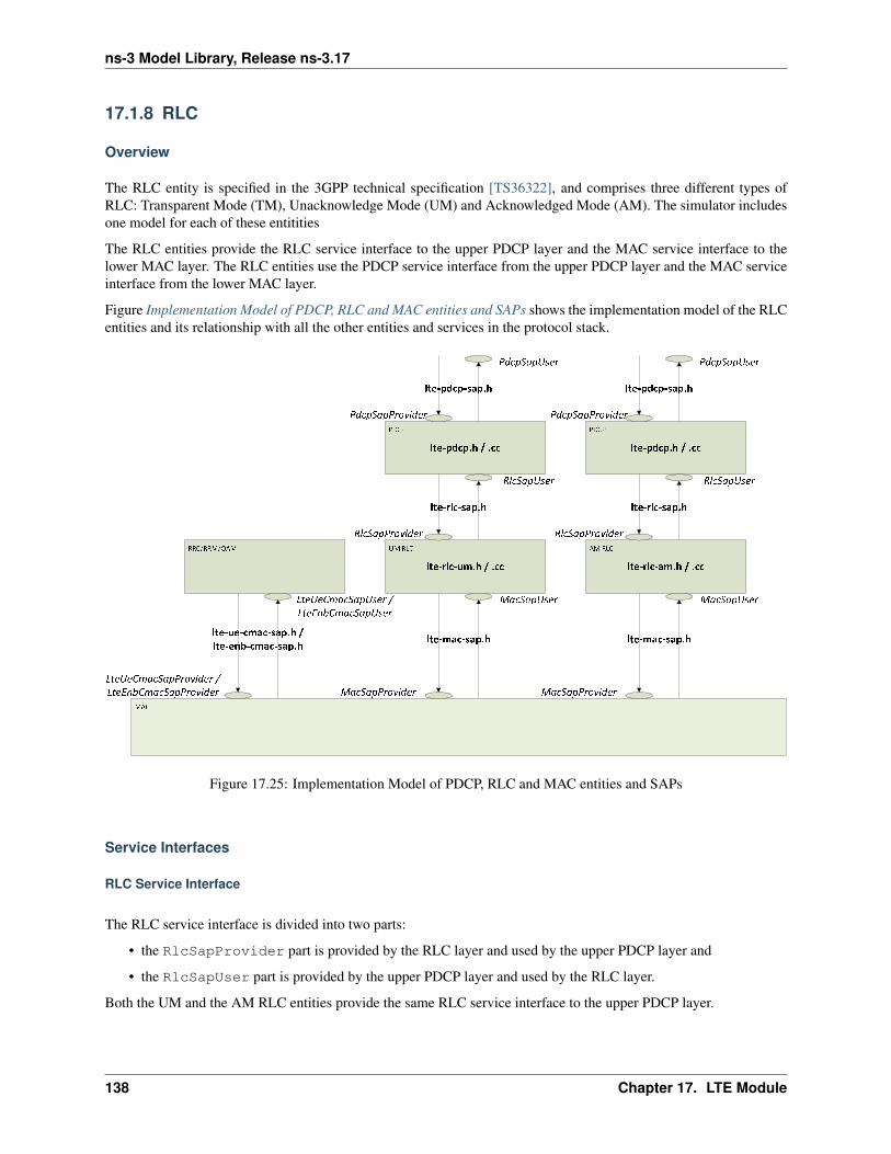
ns-3 Model Library, Release ns-3.17
17.1.8 RLC
Overview
The RLC entity is specified in the 3GPP technical specification [TS36322], and comprises three different types ofRLC: Transparent Mode (TM), Unacknowledge Mode (UM) and Acknowledged Mode (AM). The simulator includesone model for each of these entitities
The RLC entities provide the RLC service interface to the upper PDCP layer and the MAC service interface to thelower MAC layer. The RLC entities use the PDCP service interface from the upper PDCP layer and the MAC serviceinterface from the lower MAC layer.
Figure Implementation Model of PDCP, RLC and MAC entities and SAPs shows the implementation model of the RLCentities and its relationship with all the other entities and services in the protocol stack.
���
������������
������
������ ���
��� ����������������
�������������������
����������
��� �������� �����
������������� ���
��������������� �
����������������
�����������
��
������������
������ ���
�����������
������� ���
�������������
����������
������������ � ���
�������� � ���
������������
������
������ ���
�����������
��
������������
������ ���
�����������
������� ���
�������������
����������
������������ � ���
�������� � ���
Figure 17.25: Implementation Model of PDCP, RLC and MAC entities and SAPs
Service Interfaces
RLC Service Interface
The RLC service interface is divided into two parts:
• the RlcSapProvider part is provided by the RLC layer and used by the upper PDCP layer and
• the RlcSapUser part is provided by the upper PDCP layer and used by the RLC layer.
Both the UM and the AM RLC entities provide the same RLC service interface to the upper PDCP layer.
138 Chapter 17. LTE Module
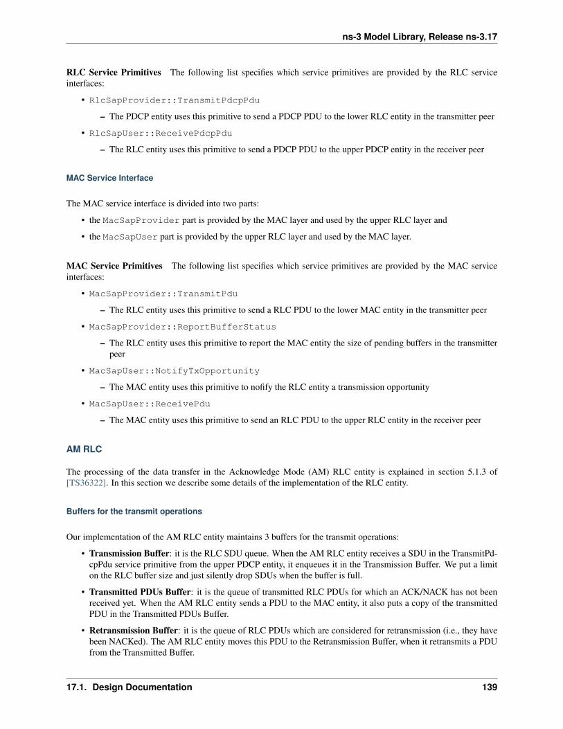
ns-3 Model Library, Release ns-3.17
RLC Service Primitives The following list specifies which service primitives are provided by the RLC serviceinterfaces:
• RlcSapProvider::TransmitPdcpPdu
– The PDCP entity uses this primitive to send a PDCP PDU to the lower RLC entity in the transmitter peer
• RlcSapUser::ReceivePdcpPdu
– The RLC entity uses this primitive to send a PDCP PDU to the upper PDCP entity in the receiver peer
MAC Service Interface
The MAC service interface is divided into two parts:
• the MacSapProvider part is provided by the MAC layer and used by the upper RLC layer and
• the MacSapUser part is provided by the upper RLC layer and used by the MAC layer.
MAC Service Primitives The following list specifies which service primitives are provided by the MAC serviceinterfaces:
• MacSapProvider::TransmitPdu
– The RLC entity uses this primitive to send a RLC PDU to the lower MAC entity in the transmitter peer
• MacSapProvider::ReportBufferStatus
– The RLC entity uses this primitive to report the MAC entity the size of pending buffers in the transmitterpeer
• MacSapUser::NotifyTxOpportunity
– The MAC entity uses this primitive to nofify the RLC entity a transmission opportunity
• MacSapUser::ReceivePdu
– The MAC entity uses this primitive to send an RLC PDU to the upper RLC entity in the receiver peer
AM RLC
The processing of the data transfer in the Acknowledge Mode (AM) RLC entity is explained in section 5.1.3 of[TS36322]. In this section we describe some details of the implementation of the RLC entity.
Buffers for the transmit operations
Our implementation of the AM RLC entity maintains 3 buffers for the transmit operations:
• Transmission Buffer: it is the RLC SDU queue. When the AM RLC entity receives a SDU in the TransmitPd-cpPdu service primitive from the upper PDCP entity, it enqueues it in the Transmission Buffer. We put a limiton the RLC buffer size and just silently drop SDUs when the buffer is full.
• Transmitted PDUs Buffer: it is the queue of transmitted RLC PDUs for which an ACK/NACK has not beenreceived yet. When the AM RLC entity sends a PDU to the MAC entity, it also puts a copy of the transmittedPDU in the Transmitted PDUs Buffer.
• Retransmission Buffer: it is the queue of RLC PDUs which are considered for retransmission (i.e., they havebeen NACKed). The AM RLC entity moves this PDU to the Retransmission Buffer, when it retransmits a PDUfrom the Transmitted Buffer.
17.1. Design Documentation 139
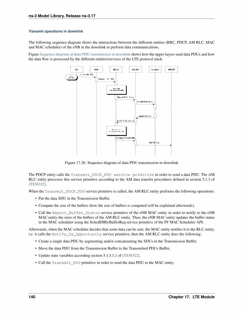
ns-3 Model Library, Release ns-3.17
Transmit operations in downlink
The following sequence diagram shows the interactions between the different entities (RRC, PDCP, AM RLC, MACand MAC scheduler) of the eNB in the downlink to perform data communications.
Figure Sequence diagram of data PDU transmission in downlink shows how the upper layers send data PDUs and howthe data flow is processed by the different entities/services of the LTE protocol stack.
��� ���� ������ �����
� ��������������
� ���������������
��� ������ �������
������������� ������
� ���������������������
� !"�#
� !"�#�# ���� �$
���������
���� ����������������� �
����������
���� ����������� �������� �
����
��� �
� !"�#�����%&�"
���'(
��"�� �"�
Figure 17.26: Sequence diagram of data PDU transmission in downlink
The PDCP entity calls the Transmit_PDCP_PDU service primitive in order to send a data PDU. The AMRLC entity processes this service primitive according to the AM data transfer procedures defined in section 5.1.3 of[TS36322].
When the Transmit_PDCP_PDU service primitive is called, the AM RLC entity performs the following operations:
• Put the data SDU in the Transmission Buffer.
• Compute the size of the buffers (how the size of buffers is computed will be explained afterwards).
• Call the Report_Buffer_Status service primitive of the eNB MAC entity in order to notify to the eNBMAC entity the sizes of the buffers of the AM RLC entity. Then, the eNB MAC entity updates the buffer statusin the MAC scheduler using the SchedDlRlcBufferReq service primitive of the FF MAC Scheduler API.
Afterwards, when the MAC scheduler decides that some data can be sent, the MAC entity notifies it to the RLC entity,i.e. it calls the Notify_Tx_Opportunity service primitive, then the AM RLC entity does the following:
• Create a single data PDU by segmenting and/or concatenating the SDUs in the Transmission Buffer.
• Move the data PDU from the Transmission Buffer to the Transmitted PDUs Buffer.
• Update state variables according section 5.1.3.1.1 of [TS36322].
• Call the Transmit_PDU primitive in order to send the data PDU to the MAC entity.
140 Chapter 17. LTE Module
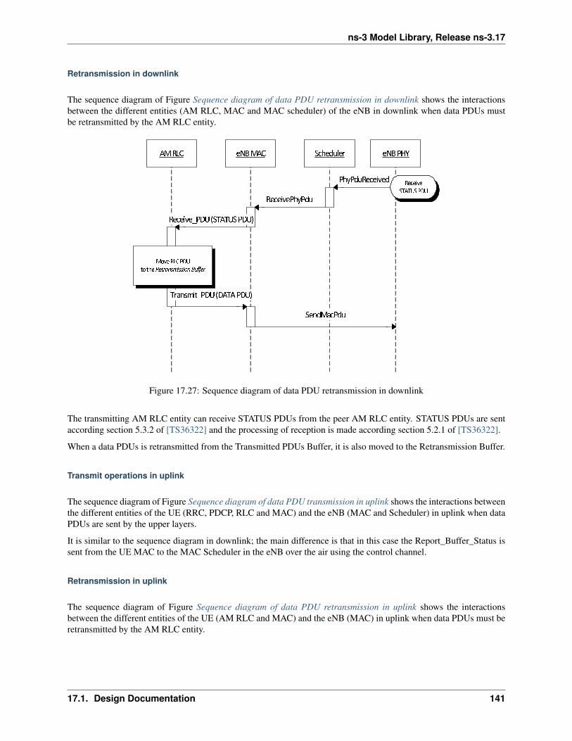
ns-3 Model Library, Release ns-3.17
Retransmission in downlink
The sequence diagram of Figure Sequence diagram of data PDU retransmission in downlink shows the interactionsbetween the different entities (AM RLC, MAC and MAC scheduler) of the eNB in downlink when data PDUs mustbe retransmitted by the AM RLC entity.
������ ������ ��� ����
����������� �
����������
���� ��������������� ����
�����������������������
����������������������
���� ��������
���� !
�������
��������
�� ���� �
Figure 17.27: Sequence diagram of data PDU retransmission in downlink
The transmitting AM RLC entity can receive STATUS PDUs from the peer AM RLC entity. STATUS PDUs are sentaccording section 5.3.2 of [TS36322] and the processing of reception is made according section 5.2.1 of [TS36322].
When a data PDUs is retransmitted from the Transmitted PDUs Buffer, it is also moved to the Retransmission Buffer.
Transmit operations in uplink
The sequence diagram of Figure Sequence diagram of data PDU transmission in uplink shows the interactions betweenthe different entities of the UE (RRC, PDCP, RLC and MAC) and the eNB (MAC and Scheduler) in uplink when dataPDUs are sent by the upper layers.
It is similar to the sequence diagram in downlink; the main difference is that in this case the Report_Buffer_Status issent from the UE MAC to the MAC Scheduler in the eNB over the air using the control channel.
Retransmission in uplink
The sequence diagram of Figure Sequence diagram of data PDU retransmission in uplink shows the interactionsbetween the different entities of the UE (AM RLC and MAC) and the eNB (MAC) in uplink when data PDUs must beretransmitted by the AM RLC entity.
17.1. Design Documentation 141
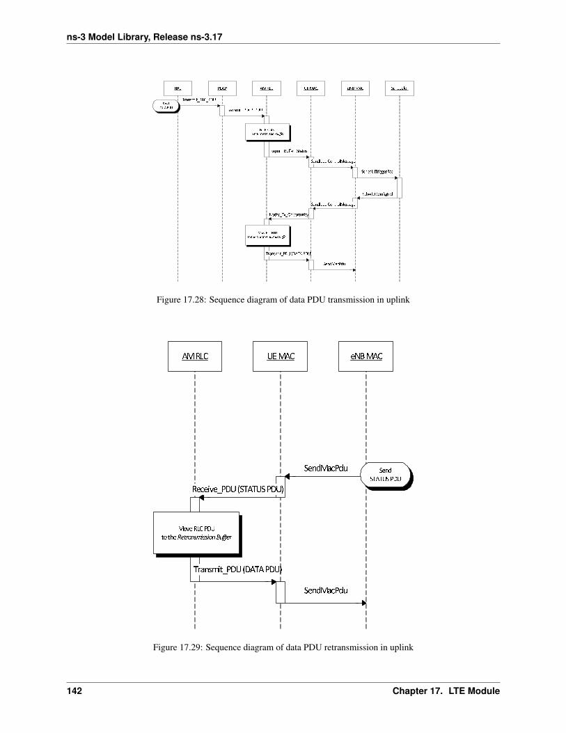
ns-3 Model Library, Release ns-3.17
��� ���� ������ �����
� ��������������
� ���������������
��� ������ �������
� ���������������������
�����
����� � �!! �"
���������
���� ����������������� �
����
����
�#����
���$�� ���� � ����!
����%��&�'��� �����%
����� �����!$��
���$�� ���� � ����!
����������
���� ����������� �������� �
���������
Figure 17.28: Sequence diagram of data PDU transmission in uplink
������ ������
����������
���� ��������������� ����
�� ������������������
�� �������
����
��������
������
����������������������
�� �������
Figure 17.29: Sequence diagram of data PDU retransmission in uplink
142 Chapter 17. LTE Module
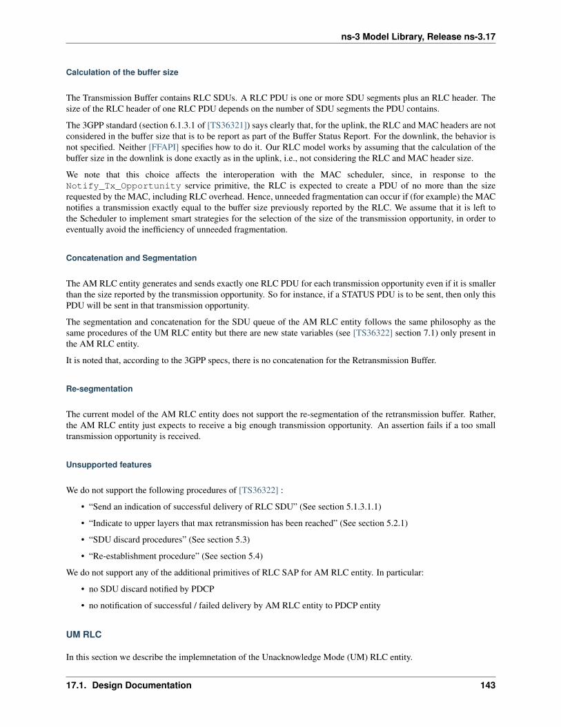
ns-3 Model Library, Release ns-3.17
Calculation of the buffer size
The Transmission Buffer contains RLC SDUs. A RLC PDU is one or more SDU segments plus an RLC header. Thesize of the RLC header of one RLC PDU depends on the number of SDU segments the PDU contains.
The 3GPP standard (section 6.1.3.1 of [TS36321]) says clearly that, for the uplink, the RLC and MAC headers are notconsidered in the buffer size that is to be report as part of the Buffer Status Report. For the downlink, the behavior isnot specified. Neither [FFAPI] specifies how to do it. Our RLC model works by assuming that the calculation of thebuffer size in the downlink is done exactly as in the uplink, i.e., not considering the RLC and MAC header size.
We note that this choice affects the interoperation with the MAC scheduler, since, in response to theNotify_Tx_Opportunity service primitive, the RLC is expected to create a PDU of no more than the sizerequested by the MAC, including RLC overhead. Hence, unneeded fragmentation can occur if (for example) the MACnotifies a transmission exactly equal to the buffer size previously reported by the RLC. We assume that it is left tothe Scheduler to implement smart strategies for the selection of the size of the transmission opportunity, in order toeventually avoid the inefficiency of unneeded fragmentation.
Concatenation and Segmentation
The AM RLC entity generates and sends exactly one RLC PDU for each transmission opportunity even if it is smallerthan the size reported by the transmission opportunity. So for instance, if a STATUS PDU is to be sent, then only thisPDU will be sent in that transmission opportunity.
The segmentation and concatenation for the SDU queue of the AM RLC entity follows the same philosophy as thesame procedures of the UM RLC entity but there are new state variables (see [TS36322] section 7.1) only present inthe AM RLC entity.
It is noted that, according to the 3GPP specs, there is no concatenation for the Retransmission Buffer.
Re-segmentation
The current model of the AM RLC entity does not support the re-segmentation of the retransmission buffer. Rather,the AM RLC entity just expects to receive a big enough transmission opportunity. An assertion fails if a too smalltransmission opportunity is received.
Unsupported features
We do not support the following procedures of [TS36322] :
• “Send an indication of successful delivery of RLC SDU” (See section 5.1.3.1.1)
• “Indicate to upper layers that max retransmission has been reached” (See section 5.2.1)
• “SDU discard procedures” (See section 5.3)
• “Re-establishment procedure” (See section 5.4)
We do not support any of the additional primitives of RLC SAP for AM RLC entity. In particular:
• no SDU discard notified by PDCP
• no notification of successful / failed delivery by AM RLC entity to PDCP entity
UM RLC
In this section we describe the implemnetation of the Unacknowledge Mode (UM) RLC entity.
17.1. Design Documentation 143
ns-3 Model Library, Release ns-3.17
Transmit operations in downlink
The transmit operations of the UM RLC are similar to those of the AM RLC previously described in Section Transmitoperations in downlink, with the difference that, following the specifications of [TS36322], retransmission are notperformed, and there are no STATUS PDUs.
Transmit operations in uplink
The transmit operations in the uplink are similar to those of the downlink, with the main difference that the Re-port_Buffer_Status is sent from the UE MAC to the MAC Scheduler in the eNB over the air using the control channel.
Calculation of the buffer size
The calculation of the buffer size for the UM RLC is done using the same approach of the AM RLC, please refer tosection Calculation of the buffer size for the corresponding description.
TM RLC
In this section we describe the implementation of the Transparent Mode (TM) RLC entity.
Transmit operations in downlink
In the simulator, the TM RLC still provides to the upper layers the same service interface provided by the AM andUM RLC entities to the PDCP layer; in practice, this interface is used by an RRC entity (not a PDCP entity) for thetransmission of RLC SDUs. This choice is motivated by the fact that the services provided by the TM RLC to theupper layers, according to [TS36322], is a subset of those provided by the UM and AM RLC entities to the PDCPlayer; hence, we reused the same interface for simplicity.
The transmit operations in the downlink are performed as follows. When the Transmit_PDCP_PDU serviceprimitive is called by the upper layers, the TM RLC does the following:
• put the SDU in the Transmission Buffer
• compute the size of the Transmission Buffer
• call the Report_Buffer_Status service primitive of the eNB MAC entity
Afterwards, when the MAC scheduler decides that some data can be sent by the logical channel to which the TM RLCentity belongs, the MAC entity notifies it to the TM RLC entity by calling the Notify_Tx_Opportunity serviceprimitive. Upon reception of this primitive, the TM RLC entity does the following:
• if the TX opportunity has a size that is greater than or equal to the size of the head-of-line SDU in the Transmis-sion Buffer
– dequeue the head-of-line SDU from the Transmission Buffer
– create one RLC PDU that contains entirely that SDU, without any RLC header
– Call the Transmit_PDU primitive in order to send the RLC PDU to the MAC entity.
144 Chapter 17. LTE Module
ns-3 Model Library, Release ns-3.17
Transmit operations in uplink
The transmit operations in the uplink are similar to those of the downlink, with the main difference that a transmissionopportunity can also arise from the assignment of the UL GRANT as part of the Random Access procedure, withoutan explicit Buffer Status Report issued by the TM RLC entity.
Calculation of the buffer size
As per the specifications [TS36322], the TM RLC does not add any RLC header to the PDUs being transmitted.Because of this, the buffer size reported to the MAC layer is calculated simply by summing the size of all packets inthe transmission buffer, thus notifying to the MAC the exact buffer size.
SM RLC
In addition to the AM, UM and TM implementations that are modeled after the 3GPP specifications, a simplified RLCmodel is provided, which is called Saturation Mode (SM) RLC. This RLC model does not accept PDUs from any abovelayer (such as PDCP); rather, the SM RLC takes care of the generation of RLC PDUs in response to the notificationof transmission opportunities notified by the MAC. In other words, the SM RLC simulates saturation conditions, i.e.,it assumes that the RLC buffer is always full and can generate a new PDU whenever notified by the scheduler.
The SM RLC is used for simplified simulation scenarios in which only the LTE Radio model is used, without the EPCand hence without any IP networking support. We note that, although the SM RLC is an unrealistic traffic model,it still allows for the correct simulation of scenarios with multiple flows belonging to different (non real-time) QoSclasses, in order to test the QoS performance obtained by different schedulers. This can be done since it is the task ofthe Scheduler to assign transmission resources based on the characteristics (e.g., Guaranteed Bit Rate) of each RadioBearer, which are specified upon the definition of each Bearer within the simulation program.
As for schedulers designed to work with real-time QoS traffic that has delay constraints, the SM RLC is probablynot an appropriate choice. This is because the absence of actual RLC SDUs (replaced by the artificial generation ofBuffer Status Reports) makes it not possible to provide the Scheduler with meaningful head-of-line-delay information,which is often the metric of choice for the implementation of scheduling policies for real-time traffic flows. For thesimulation and testing of such schedulers, it is advisable to use either the UM or the AM RLC models instead.
17.1.9 PDCP
PDCP Model Overview
The reference document for the specification of the PDCP entity is [TS36323]. With respect to this specification, thePDCP model implemented in the simulator supports only the following features:
• transfer of data (user plane or control plane);
• maintenance of PDCP SNs;
• transfer of SN status (for use upon handover);
The following features are currently not supported:
• header compression and decompression of IP data flows using the ROHC protocol;
• in-sequence delivery of upper layer PDUs at re-establishment of lower layers;
• duplicate elimination of lower layer SDUs at re-establishment of lower layers for radio bearers mapped on RLCAM;
• ciphering and deciphering of user plane data and control plane data;
17.1. Design Documentation 145
ns-3 Model Library, Release ns-3.17
• integrity protection and integrity verification of control plane data;
• timer based discard;
• duplicate discarding.
PDCP Service Interface
The PDCP service interface is divided into two parts:
• the PdcpSapProvider part is provided by the PDCP layer and used by the upper layer and
• the PdcpSapUser part is provided by the upper layer and used by the PDCP layer.
PDCP Service Primitives
The following list specifies which service primitives are provided by the PDCP service interfaces:
• PdcpSapProvider::TransmitPdcpSdu
– The RRC entity uses this primitive to send an RRC PDU to the lower PDCP entity in the transmitter peer
• PdcpSapUser::ReceivePdcpSdu
– The PDCP entity uses this primitive to send an RRC PDU to the upper RRC entity in the receiver peer
146 Chapter 17. LTE Module
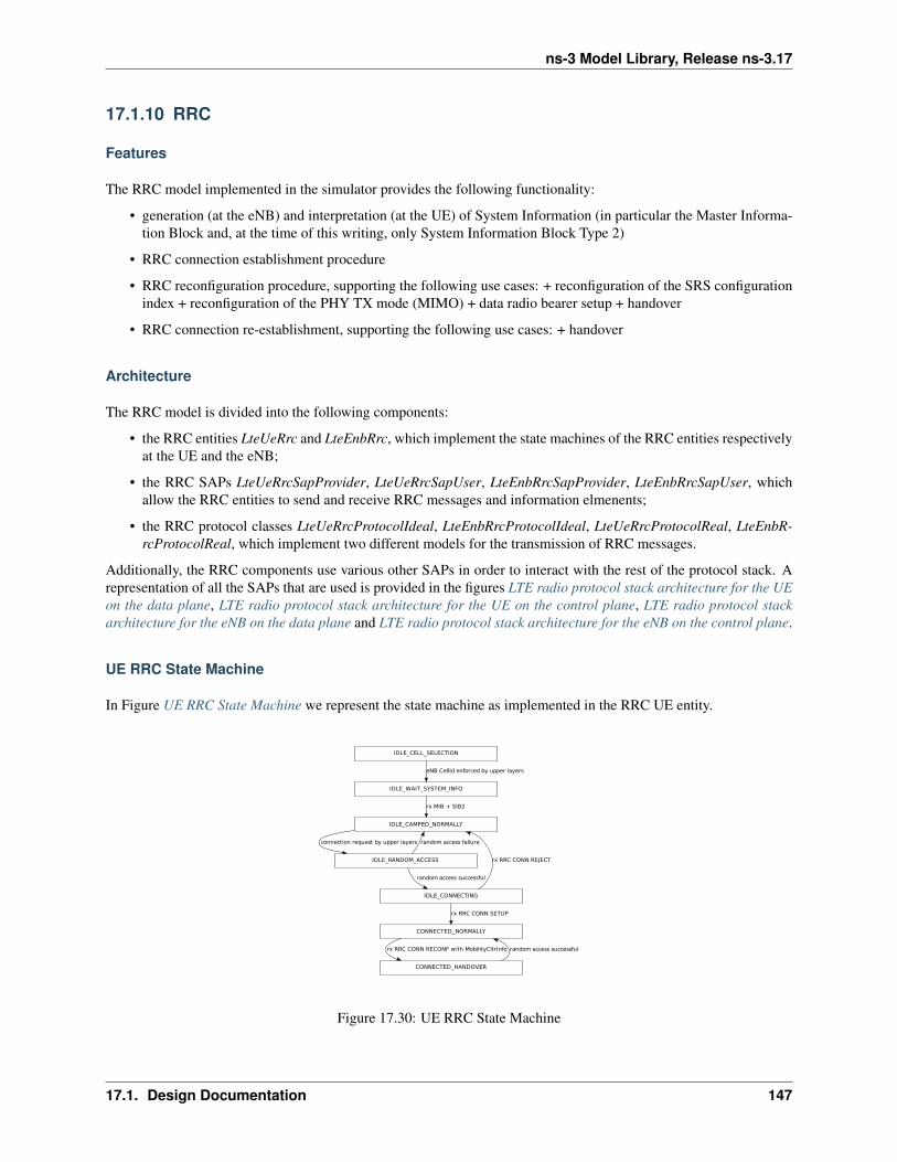
ns-3 Model Library, Release ns-3.17
17.1.10 RRC
Features
The RRC model implemented in the simulator provides the following functionality:
• generation (at the eNB) and interpretation (at the UE) of System Information (in particular the Master Informa-tion Block and, at the time of this writing, only System Information Block Type 2)
• RRC connection establishment procedure
• RRC reconfiguration procedure, supporting the following use cases: + reconfiguration of the SRS configurationindex + reconfiguration of the PHY TX mode (MIMO) + data radio bearer setup + handover
• RRC connection re-establishment, supporting the following use cases: + handover
Architecture
The RRC model is divided into the following components:
• the RRC entities LteUeRrc and LteEnbRrc, which implement the state machines of the RRC entities respectivelyat the UE and the eNB;
• the RRC SAPs LteUeRrcSapProvider, LteUeRrcSapUser, LteEnbRrcSapProvider, LteEnbRrcSapUser, whichallow the RRC entities to send and receive RRC messages and information elmenents;
• the RRC protocol classes LteUeRrcProtocolIdeal, LteEnbRrcProtocolIdeal, LteUeRrcProtocolReal, LteEnbR-rcProtocolReal, which implement two different models for the transmission of RRC messages.
Additionally, the RRC components use various other SAPs in order to interact with the rest of the protocol stack. Arepresentation of all the SAPs that are used is provided in the figures LTE radio protocol stack architecture for the UEon the data plane, LTE radio protocol stack architecture for the UE on the control plane, LTE radio protocol stackarchitecture for the eNB on the data plane and LTE radio protocol stack architecture for the eNB on the control plane.
UE RRC State Machine
In Figure UE RRC State Machine we represent the state machine as implemented in the RRC UE entity.
IDLE_CELL_SELECTION
IDLE_WAIT_SYSTEM_INFO
eNB CellId enforced by upper layers
IDLE_CAMPED_NORMALLY
rx MIB + SIB2
IDLE_RANDOM_ACCESS
connection request by upper layers random access failure
IDLE_CONNECTING
random access successful
rx RRC CONN REJECT
CONNECTED_NORMALLY
rx RRC CONN SETUP
CONNECTED_HANDOVER
rx RRC CONN RECONF with MobilityCltrInfo random access successful
Figure 17.30: UE RRC State Machine
17.1. Design Documentation 147
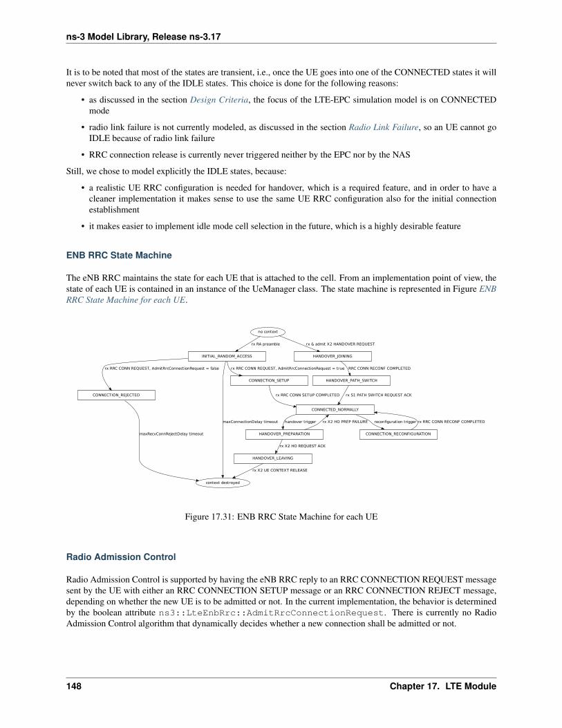
ns-3 Model Library, Release ns-3.17
It is to be noted that most of the states are transient, i.e., once the UE goes into one of the CONNECTED states it willnever switch back to any of the IDLE states. This choice is done for the following reasons:
• as discussed in the section Design Criteria, the focus of the LTE-EPC simulation model is on CONNECTEDmode
• radio link failure is not currently modeled, as discussed in the section Radio Link Failure, so an UE cannot goIDLE because of radio link failure
• RRC connection release is currently never triggered neither by the EPC nor by the NAS
Still, we chose to model explicitly the IDLE states, because:
• a realistic UE RRC configuration is needed for handover, which is a required feature, and in order to have acleaner implementation it makes sense to use the same UE RRC configuration also for the initial connectionestablishment
• it makes easier to implement idle mode cell selection in the future, which is a highly desirable feature
ENB RRC State Machine
The eNB RRC maintains the state for each UE that is attached to the cell. From an implementation point of view, thestate of each UE is contained in an instance of the UeManager class. The state machine is represented in Figure ENBRRC State Machine for each UE.
no context
INITIAL_RANDOM_ACCESS
rx RA preamble
HANDOVER_JOINING
rx & admit X2 HANDOVER REQUEST
CONNECTION_SETUP
rx RRC CONN REQUEST, AdmitRrcConnectionRequest = true
CONNECTION_REJECTED
rx RRC CONN REQUEST, AdmitRrcConnectionRequest = false
context destroyed
maxConnectionDelay timeout
CONNECTED_NORMALLY
rx RRC CONN SETUP COMPLETED
maxRecvConnRejectDelay timeout CONNECTION_RECONFIGURATION
reconfiguration trigger
HANDOVER_PREPARATION
handover trigger rx RRC CONN RECONF COMPLETEDrx X2 HO PREP FAILURE
HANDOVER_LEAVING
rx X2 HO REQUEST ACK
HANDOVER_PATH_SWITCH
RRC CONN RECONF COMPLETED
rx S1 PATH SWITCH REQUEST ACK
rx X2 UE CONTEXT RELEASE
Figure 17.31: ENB RRC State Machine for each UE
Radio Admission Control
Radio Admission Control is supported by having the eNB RRC reply to an RRC CONNECTION REQUEST messagesent by the UE with either an RRC CONNECTION SETUP message or an RRC CONNECTION REJECT message,depending on whether the new UE is to be admitted or not. In the current implementation, the behavior is determinedby the boolean attribute ns3::LteEnbRrc::AdmitRrcConnectionRequest. There is currently no RadioAdmission Control algorithm that dynamically decides whether a new connection shall be admitted or not.
148 Chapter 17. LTE Module
ns-3 Model Library, Release ns-3.17
Radio Bearer Configuration
Some implementation choices have been made in the RRC regarding the setup of radio bearers:
• three Logical Channel Groups (out of four available) are configured for uplink buffer status report purposes,according to the following policy:
– LCG 0 is for signaling radio bearers
– LCG 1 is for GBR data radio bearers
– LCG 2 is for Non-GBR data radio bearers
Radio Link Failure
Since at this stage the RRC supports the CONNECTED mode only, Radio Link Failure (RLF) is not handled. Thereason is that one of the possible outcomes of RLF (when RRC re-establishment is unsuccessful) is to leave RRCCONNECTED notifying the NAS of the RRC connection failure. In order to model RLF properly, RRC IDLE modeshould be supported, including in particular idle mode cell (re-)selection.
With the current model, an UE that experiences bad link quality will just stay associated with the same eNB, and thescheduler will stop allocating resources to it for communications. This is also consistent with the fact that, at this stage,only handovers explicitly triggered within the simulation program are supported (network-driven handovers based onUE measurements are planned only at a later stage).
Handover
The RRC model support the execution of an X2-based handover procedure. The handover needs to be triggered explic-itly by the simulation program by scheduling an execution of the method LteEnbRrc::SendHandoverRequest(). The automatic triggering of the handover based on UE measurements is not supported at this stage.
RRC sequence diagrams
In this section we provide some sequence diagrams that explain the most important RRC procedures being modeled.
RRC connection establishment
Figure Sequence diagram of the RRC Connection Establishment procedure shows how the RRC Connection Estab-lishment procedure is modeled, highlighting the role of the RRC layer at both the UE and the eNB, as well as theinteraction with the other layers.
RRC connection reconfiguration
Figure Sequence diagram of the RRC Connection Reconfiguration procedure shows how the RRC Connection Re-configuration procedure is modeled for the case where MobilityControlInfo is not provided, i.e., handover is notperformed.
Figure Sequence diagram of the RRC Connection Reconfiguration procedure for the handover case shows how theRRC Connection Reconfiguration procedure is modeled for the case where MobilityControlInfo is provided, i.e.,handover is to be performed. As specified in [TS36331], After receiving the handover message, the UE attempts toaccess the target cell at the first available RACH occasion according to Random Access resource selection defined in[TS36321]_, i.e. the handover is asynchronous. Consequently, when allocating a dedicated preamble for the randomaccess in the target cell, E-UTRA shall ensure it is available from the first RACH occasion the UE may use. Upon
17.1. Design Documentation 149
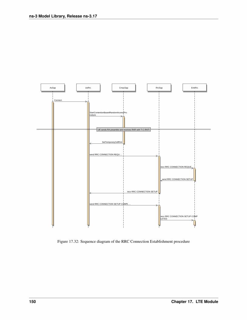
ns-3 Model Library, Release ns-3.17
AsSap UeRrc CmacSap RrcSap EnbRrc
Connect
StartContentionBasedRandomAccessProcedure
SetTemporaryCellRnti
send RRC CONNECTION REQU ...
recv RRC CONNECTION REQUE ...
send RRC CONNECTION SETUP
recv RRC CONNECTION SETUP
send RRC CONNECTION SETUP COMPL ...
recv RRC CONNECTION SETUP COMPLETED
UE sends RA preamble and receives RAR with T-C-RNTI
Figure 17.32: Sequence diagram of the RRC Connection Establishment procedure
150 Chapter 17. LTE Module
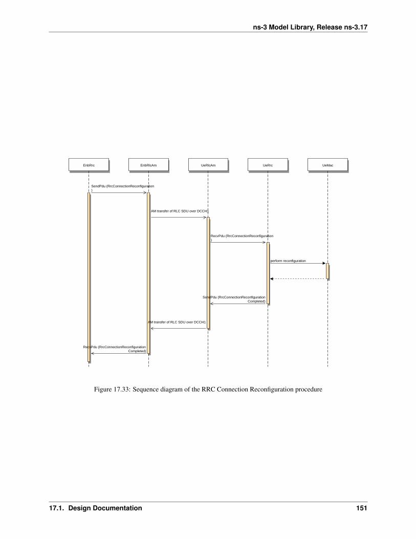
ns-3 Model Library, Release ns-3.17
EnbRrc EnbRlcAm UeRlcAm UeRrc UeMac
SendPdu (RrcConnectionReconfiguration)
AM transfer of RLC SDU over DCCH1
RecvPdu (RrcConnectionReconfiguration)
perform reconfiguration
SendPdu (RrcConnectionReconfigurationCompleted)
AM transfer of RLC SDU over DCCH1
RecvPdu (RrcConnectionReconfigurationCompleted)
Figure 17.33: Sequence diagram of the RRC Connection Reconfiguration procedure
17.1. Design Documentation 151
ns-3 Model Library, Release ns-3.17
successful completion of the handover, the UE sends a message used to confirm the handover. Note that the randomaccess procedure in this case is non-contention based, hence in a real LTE system it differs slightly from the one usedin RRC connection established. Also note that the RA Preamble ID is signalled via the Handover Command includedin the X2 Handover Request ACK message sent from the target eNB to the source eNB; in particular, the preamble isincluded in the RACH-ConfigDedicated IE which is part of MobilityControlInfo.
RRC protocol models
As previously anticipated, we provide two different models for the transmission and reception of RRC messages: Idealand Real. Each of them is described in one of the following subsections.
Ideal RRC protocol model
According to this model, implemented in the classes and LteUeRrcProtocolIdeal and LteEnbRrcProtocolIdeal, allRRC messages and information elements are transmitted between the eNB and the UE in an ideal fashion, withoutconsuming radio resources and without errors. From an implementation point of view, this is achieved by passing theRRC data structure directly between the UE and eNB RRC entities, without involving the lower layers (PDCP, RLC,MAC, scheduler).
Real RRC protocol model
This model is implemented in the classes LteUeRrcProtocolReal and LteEnbRrcProtocolReal and aims at modelingthe transmission of RRC PDUs as commonly performed in real LTE systems. In particular:
• for every RRC message being sent, a real RRC PDUs is created following the ASN.1 encoding of RRC PDUsand information elements (IEs) specified in [TS36331]. Some simplification are made with respect to the IEsincluded in the PDU, i.e., only those IEs that are useful for simulation purposes are included. For a detailed list,please see the IEs defined in lte-rrc-sap.h and compare with [TS36331].
• the encoded RRC PDUs are sent on Signaling Radio Bearers and are subject to the same transmission modelingused for data communications, thus including scheduling, radio resource consumption, channel errors, delays,retransmissions, etc.
Signaling Radio Bearer model We now describe the Signaling Radio Bearer model that is used for the Real RRCprotocol model.
• SRB0 messages (over CCCH):
– RrcConnectionRequest: in real LTE systems, this is an RLC TM SDU sent over resources specified inthe UL Grant in the RAR (not in UL DCIs); the reason is that C-RNTI is not known yet at this stage. Inthe simulator, this is modeled as a real RLC TM RLC PDU whose UL resources are allocated by the schedupon call to SCHED_DL_RACH_INFO_REQ.
– RrcConnectionSetup: in the simulator this is implemented as in real LTE systems, i.e.,with an RLC TM SDU sent over resources indicated by a regular UL DCI, allocated withSCHED_DL_RLC_BUFFER_REQ triggered by the RLC TM instance that is mapped to LCID 0 (theCCCH).
• SRB1 messages (over DCCH):
– All the SRB1 messages modeled in the simulator (e.g., RrcConnectionCompleted) are implemented as inreal LTE systems, i.e., with a real RLC SDU sent over RLC AM using DL resources allocated via BufferStatus Reports. See the RLC model documentation for details.
• SRB2 messages (over DCCH):
152 Chapter 17. LTE Module
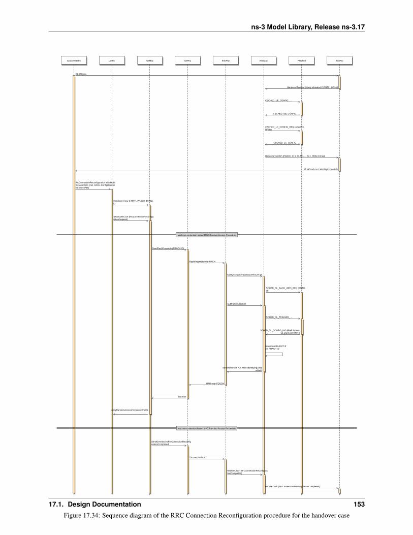
ns-3 Model Library, Release ns-3.17
sourceEnbRrc UeRrc UeMac UePhy EnbPhy EnbMac FfSched EnbRrc
X2: HO req
HandoverRequest (newly allocated C-RNTI + LC list)
CSCHED_UE_CONFIG_ ...
CSCHED_UE_CONFIG_ ...
CSCHED_LC_CONFIG_REQ (all active DRBs)
CSCHED_LC_CONFIG_ ...
HandoverConfirm (PRACH ID in 63-Ncf,..., 63 + PRACH mask
X2: HO ack incl. MobilityControlInfo
RrcConnectionReconfiguration with MobilityControlInfo (incl. RACH-ConfigDedicated over SRB1
Handover (new C-RNTI, PRACH ID+Mask)
SendOverCcch (RrcConnectionReconfigurationRequest)
SendRachPreamble (PRACH ID)
RachPreamble over RACH
NotifyRxRachPreamble (PRACH ID)
SCHED_DL_RACH_INFO_REQ (RNTI list)
SubframeIndication
SCHED_DL_TRIGGER_ ...
SCHED_DL_CONFIG_IND (RAR list withUL grant per RNTI))
determine RA-RNTI from PRACH ID
Send RAR with RA-RNTI identifying preambleId
RAR over PDSCH
Rx RAR
NotifyRandomAccessProcedureEndOk
SendOverUlsch (RrcConnectionReconfigurationCompleted)
TX over PUSCH
RxOverUlsch (RrcConnectionReconfigurationCompleted)
RxOverCcch (RrcConnectionReconfigurationCompleted)
start non-contention based MAC Random Access Procedure
end non-contention based MAC Random Access Procedure
Figure 17.34: Sequence diagram of the RRC Connection Reconfiguration procedure for the handover case
17.1. Design Documentation 153
ns-3 Model Library, Release ns-3.17
– According to [TS36331], “SRB1 is for RRC messages (which may include a piggybacked NAS message) aswell as for NAS messages prior to the establishment of SRB2, all using DCCH logical channel”, whereas“SRB2 is for NAS messages, using DCCH logical channel” and “SRB2 has a lower-priority than SRB1 andis always configured by E-UTRAN after security activation”. Modeling security-related aspects is not arequirement of the LTE simulation model, hence we always use SRB1 and never activate SRB2.
ASN.1 encoding of RRC IE’s The messages defined in RRC SAP, common to all Ue/Enb SAP Users/Providers, aretransported in a transparent container to/from a Ue/Enb. The encoding format for the different Information Elementsare specified in [TS36331], using ASN.1 rules in the unaligned variant. The implementation in Ns3/Lte has beendivided in the following classes:
• Asn1Header : Contains the encoding / decoding of basic ASN types
• RrcAsn1Header : Inherits Asn1Header and contains the encoding / decoding of common IE’s defined in[TS36331]
• Rrc specific messages/IEs classes : A class for each of the messages defined in RRC SAP header
Asn1Header class - Implementation of base ASN.1 types This class implements the methods to Serialize / Dese-rialize the ASN.1 types being used in [TS36331], according to the packed encoding rules in ITU-T X.691. The typesconsidered are:
• Boolean : a boolean value uses a single bit (1=true, 0=false).
• Integer : a constrained integer (with min and max values defined) uses the minimum amount of bits to encodeits range (max-min+1).
• Bitstring : a bistring will be copied bit by bit to the serialization buffer.
• Octetstring : not being currently used.
• Sequence : the sequence generates a preamble indicating the presence of optional and default fields. It also addsa bit indicating the presence of extension marker.
• Sequence...Of : the sequence...of type encodes the number of elements of the sequence as an integer (the subse-quent elements will need to be encoded afterwards).
• Choice : indicates which element among the ones in the choice set is being encoded.
• Enumeration : is serialized as an integer indicating which value is used, among the ones in the enumeration,with the number of elements in the enumeration as upper bound.
• Null : the null value is not encoded, although its serialization function is defined to provide a clearer mapbetween specification and implementation.
The class inherits from ns-3 Header, but Deserialize() function is declared pure virtual, thus inherited classes having toimplement it. The reason is that deserialization will retrieve the elements in RRC messages, each of them containingdifferent information elements.
Additionally, it has to be noted that the resulting byte length of a specific type/message can vary, according to thepresence of optional fields, and due to the optimized encoding. Hence, the serialized bits will be processed usingPreSerialize() function, saving the result in m_serializationResult Buffer. As the methods to read/write in a ns3 bufferare defined in a byte basis, the serialization bits are stored into m_serializationPendingBits attribute, until the 8 bits areset and can be written to buffer iterator. Finally, when invoking Serialize(), the contents of the m_serializationResultattribute will be copied to Buffer::Iterator parameter
RrcAsn1Header : Common IEs As some Information Elements are being used for several RRC messages, thisclass implements the following common IE’s:
154 Chapter 17. LTE Module

ns-3 Model Library, Release ns-3.17
• SrbToAddModList
• DrbToAddModList
• LogicalChannelConfig
• RadioResourceConfigDedicated
• PhysicalConfigDedicated
• SystemInformationBlockType1
• SystemInformationBlockType2
• RadioResourceConfigCommonSIB
Rrc specific messages/IEs classes The following RRC SAP have been implemented:
• RrcConnectionRequest
• RrcConnectionSetup
• RrcConnectionSetupCompleted
• RrcConnectionReconfiguration
• RrcConnectionReconfigurationCompleted
• HandoverPreparationInfo
• RrcConnectionReestablishmentRequest
• RrcConnectionReestablishment
• RrcConnectionReestablishmentComplete
• RrcConnectionReestablishmentReject
• RrcConnectionRelease
17.1. Design Documentation 155

ns-3 Model Library, Release ns-3.17
17.1.11 NAS
The focus of the LTE-EPC model is on the NAS Active state, which corresponds to EMM Registered, ECM connected,and RRC connected. Because of this, the following simplifications are made:
• EMM and ECM are not modeled explicitly; instead, the NAS entity at the UE will interact directy with the MMEto perfom actions that are equivalent (with gross simplifications) to taking the UE to the states EMM Connectedand ECM Connected;
• the NAS also takes care of multiplexing uplink data packets coming from the upper layers into the appropriateEPS bearer by using the Traffic Flow Template classifier (TftClassifier).
• the NAS does not support PLMN and CSG selection
• the NAS does not support any location update/paging procedure in idle mode
Figure Sequence diagram of the attach procedure shows how the simplified NAS model implements the attach proce-dure. Note that both the default and eventual dedicated EPS bearers are activated as part of this procedure.
156 Chapter 17. LTE Module
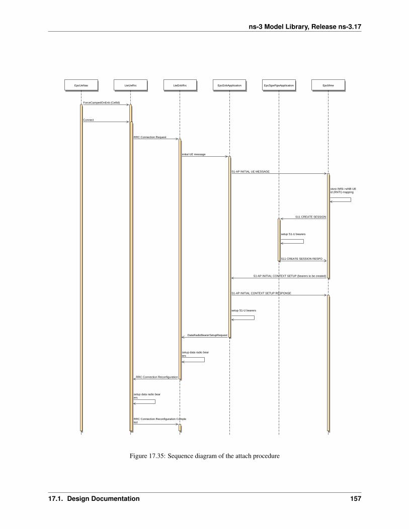
ns-3 Model Library, Release ns-3.17
EpcUeNas LteUeRrc LteEnbRrc EpcEnbApplication EpcSgwPgwApplication EpcMme
ForceCampedOnEnb (CellId)
Connect
RRC Connection Request
initial UE message
S1-AP INITIAL UE MESSAGE
store IMSI->eNB UEid (RNTI) mapping
S11 CREATE SESSION
setup S1-U bearers
S11 CREATE SESSION RESPO ...
S1-AP INITIAL CONTEXT SETUP (bearers to be created)
S1-AP INITIAL CONTEXT SETUP RESPONSE
setup S1-U bearers
DataRadioBearerSetupRequest
setup data radio bearers
RRC Connection Reconfiguration
setup data radio bearers
RRC Connection Reconfiguration Completed
Figure 17.35: Sequence diagram of the attach procedure
17.1. Design Documentation 157
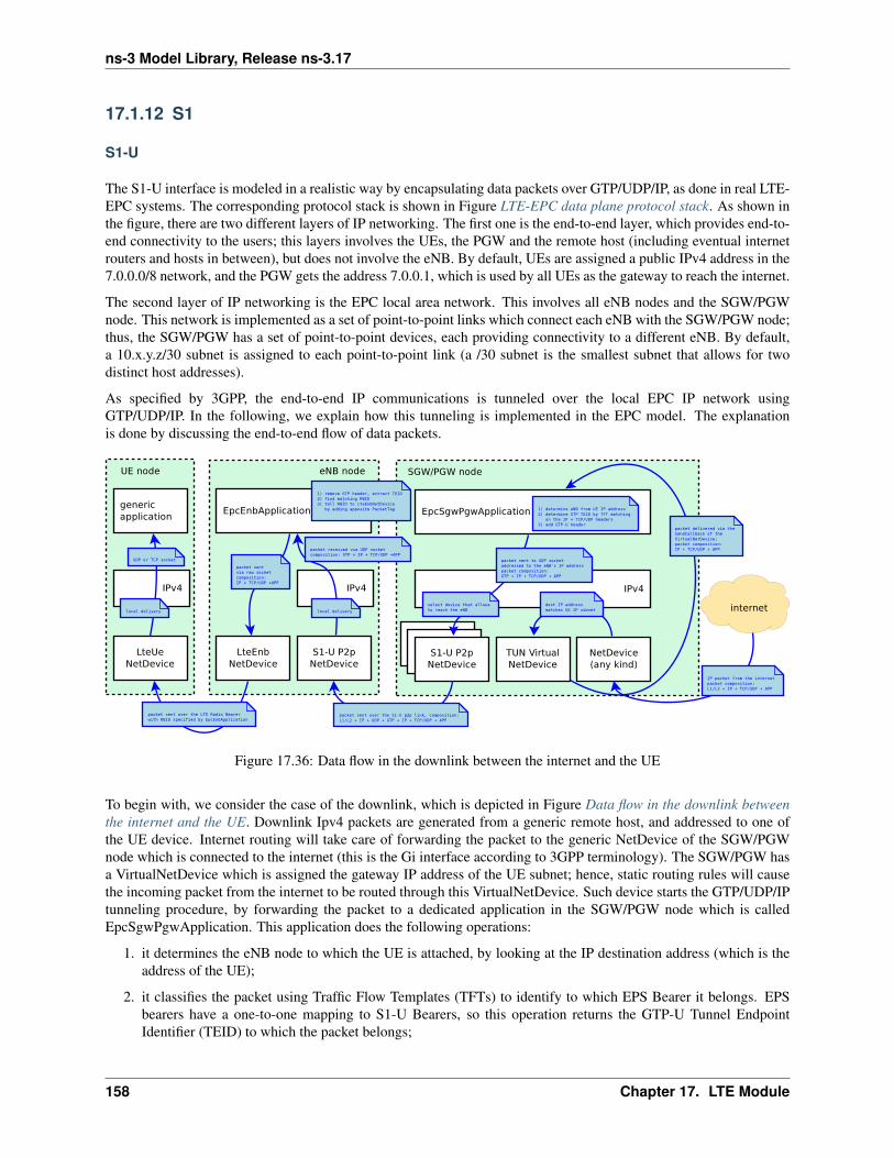
ns-3 Model Library, Release ns-3.17
17.1.12 S1
S1-U
The S1-U interface is modeled in a realistic way by encapsulating data packets over GTP/UDP/IP, as done in real LTE-EPC systems. The corresponding protocol stack is shown in Figure LTE-EPC data plane protocol stack. As shown inthe figure, there are two different layers of IP networking. The first one is the end-to-end layer, which provides end-to-end connectivity to the users; this layers involves the UEs, the PGW and the remote host (including eventual internetrouters and hosts in between), but does not involve the eNB. By default, UEs are assigned a public IPv4 address in the7.0.0.0/8 network, and the PGW gets the address 7.0.0.1, which is used by all UEs as the gateway to reach the internet.
The second layer of IP networking is the EPC local area network. This involves all eNB nodes and the SGW/PGWnode. This network is implemented as a set of point-to-point links which connect each eNB with the SGW/PGW node;thus, the SGW/PGW has a set of point-to-point devices, each providing connectivity to a different eNB. By default,a 10.x.y.z/30 subnet is assigned to each point-to-point link (a /30 subnet is the smallest subnet that allows for twodistinct host addresses).
As specified by 3GPP, the end-to-end IP communications is tunneled over the local EPC IP network usingGTP/UDP/IP. In the following, we explain how this tunneling is implemented in the EPC model. The explanationis done by discussing the end-to-end flow of data packets.
Figure 17.36: Data flow in the downlink between the internet and the UE
To begin with, we consider the case of the downlink, which is depicted in Figure Data flow in the downlink betweenthe internet and the UE. Downlink Ipv4 packets are generated from a generic remote host, and addressed to one ofthe UE device. Internet routing will take care of forwarding the packet to the generic NetDevice of the SGW/PGWnode which is connected to the internet (this is the Gi interface according to 3GPP terminology). The SGW/PGW hasa VirtualNetDevice which is assigned the gateway IP address of the UE subnet; hence, static routing rules will causethe incoming packet from the internet to be routed through this VirtualNetDevice. Such device starts the GTP/UDP/IPtunneling procedure, by forwarding the packet to a dedicated application in the SGW/PGW node which is calledEpcSgwPgwApplication. This application does the following operations:
1. it determines the eNB node to which the UE is attached, by looking at the IP destination address (which is theaddress of the UE);
2. it classifies the packet using Traffic Flow Templates (TFTs) to identify to which EPS Bearer it belongs. EPSbearers have a one-to-one mapping to S1-U Bearers, so this operation returns the GTP-U Tunnel EndpointIdentifier (TEID) to which the packet belongs;
158 Chapter 17. LTE Module
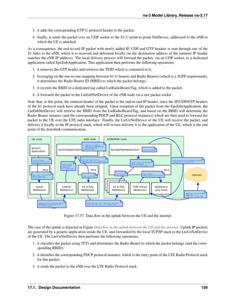
ns-3 Model Library, Release ns-3.17
3. it adds the corresponding GTP-U protocol header to the packet;
4. finally, it sends the packet over an UDP socket to the S1-U point-to-point NetDevice, addressed to the eNB towhich the UE is attached.
As a consequence, the end-to-end IP packet with newly added IP, UDP and GTP headers is sent through one of theS1 links to the eNB, where it is received and delivered locally (as the destination address of the outmost IP headermatches the eNB IP address). The local delivery process will forward the packet, via an UDP socket, to a dedicatedapplication called EpcEnbApplication. This application then performs the following operations:
1. it removes the GTP header and retrieves the TEID which is contained in it;
2. leveraging on the one-to-one mapping between S1-U bearers and Radio Bearers (which is a 3GPP requirement),it determines the Radio Bearer ID (RBID) to which the packet belongs;
3. it records the RBID in a dedicated tag called LteRadioBearerTag, which is added to the packet;
4. it forwards the packet to the LteEnbNetDevice of the eNB node via a raw packet socket
Note that, at this point, the outmost header of the packet is the end-to-end IP header, since the IP/UDP/GTP headersof the S1 protocol stack have already been stripped. Upon reception of the packet from the EpcEnbApplication, theLteEnbNetDevice will retrieve the RBID from the LteRadioBearerTag, and based on the RBID will determine theRadio Bearer instance (and the corresponding PDCP and RLC protocol instances) which are then used to forward thepacket to the UE over the LTE radio interface. Finally, the LteUeNetDevice of the UE will receive the packet, anddelivery it locally to the IP protocol stack, which will in turn delivery it to the application of the UE, which is the endpoint of the downlink communication.
Figure 17.37: Data flow in the uplink between the UE and the internet
The case of the uplink is depicted in Figure Data flow in the uplink between the UE and the internet. Uplink IP packetsare generated by a generic application inside the UE, and forwarded by the local TCP/IP stack to the LteUeNetDeviceof the UE. The LteUeNetDevice then performs the following operations:
1. it classifies the packet using TFTs and determines the Radio Bearer to which the packet belongs (and the corre-sponding RBID);
2. it identifies the corresponding PDCP protocol instance, which is the entry point of the LTE Radio Protocol stackfor this packet;
3. it sends the packet to the eNB over the LTE Radio Protocol stack.
17.1. Design Documentation 159
ns-3 Model Library, Release ns-3.17
The eNB receives the packet via its LteEnbNetDevice. Since there is a single PDCP and RLC protocol instance foreach Radio Bearer, the LteEnbNetDevice is able to determine the RBID of the packet. This RBID is then recordedonto an LteRadioBearerTag, which is added to the packet. The LteEnbNetDevice then forwards the packet to theEpcEnbApplication via a raw packet socket.
Upon receiving the packet, the EpcEnbApplication performs the following operations:
1. it retrieves the RBID from the LteRadioBearerTag in the packet;
2. it determines the corresponding EPS Bearer instance and GTP-U TEID by leveraging on the one-to-one mappingbetween S1-U bearers and Radio Bearers;
3. it adds a GTP-U header on the packet, including the TEID determined previously;
4. it sends the packet to the SGW/PGW node via the UDP socket connected to the S1-U point-to-point net device.
At this point, the packet contains the S1-U IP, UDP and GTP headers in addition to the original end-to-end IP header.When the packet is received by the corresponding S1-U point-to-point NetDevice of the SGW/PGW node, it is deliv-ered locally (as the destination address of the outmost IP header matches the address of the point-to-point net device).The local delivery process will forward the packet to the EpcSgwPgwApplication via the correponding UDP socket.The EpcSgwPgwApplication then removes the GTP header and forwards the packet to the VirtualNetDevice. At thispoint, the outmost header of the packet is the end-to-end IP header. Hence, if the destination address within this headeris a remote host on the internet, the packet is sent to the internet via the corresponding NetDevice of the SGW/PGW.In the event that the packet is addressed to another UE, the IP stack of the SGW/PGW will redirect the packet againto the VirtualNetDevice, and the packet will go through the dowlink delivery process in order to reach its destinationUE.
Note that the EPS Bearer QoS is not enforced on the S1-U links, it is assumed that the overprovisioning of the linkbandwidth is sufficient to meet the QoS requirements of all bearers.
S1AP
The S1-AP interface provides control plane interaction between the eNB and the MME. In the simulator, this inter-face is modeled in an ideal fashion, with direct interaction between the eNB and the MME objects, without actuallyimplementing the encoding of S1AP messages and information elements specified in [TS36413] and without actuallytransmitting any PDU on any link.
The S1-AP primitives that are modeled are:
• INITIAL UE MESSAGE
• INITIAL CONTEXT SETUP REQUEST
• INITIAL CONTEXT SETUP RESPONSE
• PATH SWITCH REQUEST
• PATH SWITCH REQUEST ACKNOWLEDGE
160 Chapter 17. LTE Module

ns-3 Model Library, Release ns-3.17
17.1.13 X2
The X2 interface interconnects two eNBs [TS36420]. From a logical point of view, the X2 interface is a point-to-pointinterface between the two eNBs. In a real E-UTRAN, the logical point-to-point interface should be feasible even inthe absence of a physical direct connection between the two eNBs. In the X2 model implemented in the simulator, theX2 interface is a point-to-point link between the two eNBs. A point-to-point device is created in both eNBs and thetwo point-to-point devices are attached to the point-to-point link.
For a representation of how the X2 interface fits in the overall architecture of the LENA simulation model, the readeris referred to the figure Architecture.
The X2 interface implemented in the simulator provides detailed implementation of the following elementary proce-dures of the Mobility Management functionality [TS36423]:
• Handover Request procedure
• Handover Request Acknowledgement procedure
• SN Status Transfer procedure
• UE Context Release procedure
These procedures are involved in the X2-based handover. You can find the detailed description of the handover insection 10.1.2.1 of [TS36300]. We note that the simulator model currently supports only the seamless handover asdefined in Section 2.6.3.1 of [Sesia2009]; in particular, lossless handover as described in Section 2.6.3.2 of [Sesia2009]is not supported at the time of this writing.
Figure Sequence diagram of the X2-based handover shows the interaction of the entities of the X2 model in thesimulator.
The X2 model is an entity that uses services from:
• the X2 interfaces,
– They are implemented as Sockets on top of the point-to-point devices.
– They are used to send/receive X2 messages through the X2-C and X2-U interfaces (i.e. the point-to-pointdevice attached to the point-to-point link) towards the peer eNB.
• the S1 application.
– Currently, it is the EpcEnbApplication.
– It is used to get some information needed for the Elementary Procedures of the X2 messages.
and it provides services to:
• the RRC entity (X2 SAP)
– to send/receive RRC messages. The X2 entity sends the RRC message as a transparent container in the X2message. This RRC message is sent to the UE.
Figure Implementation Model of X2 entity and SAPs shows the implentation model of the X2 entity and its relationshipwith all the other entities and services in the protocol stack.
The RRC entity manages the initiation of the handover procedure. This is done in the Handover Management sub-module of the eNB RRC entity. The target eNB may perform some Admission Control procedures. This is done in theAdmission Control submodule. Initially, this submodule will accept any handover request.
X2 interfaces
The X2 model contains two interfaces:
17.1. Design Documentation 161
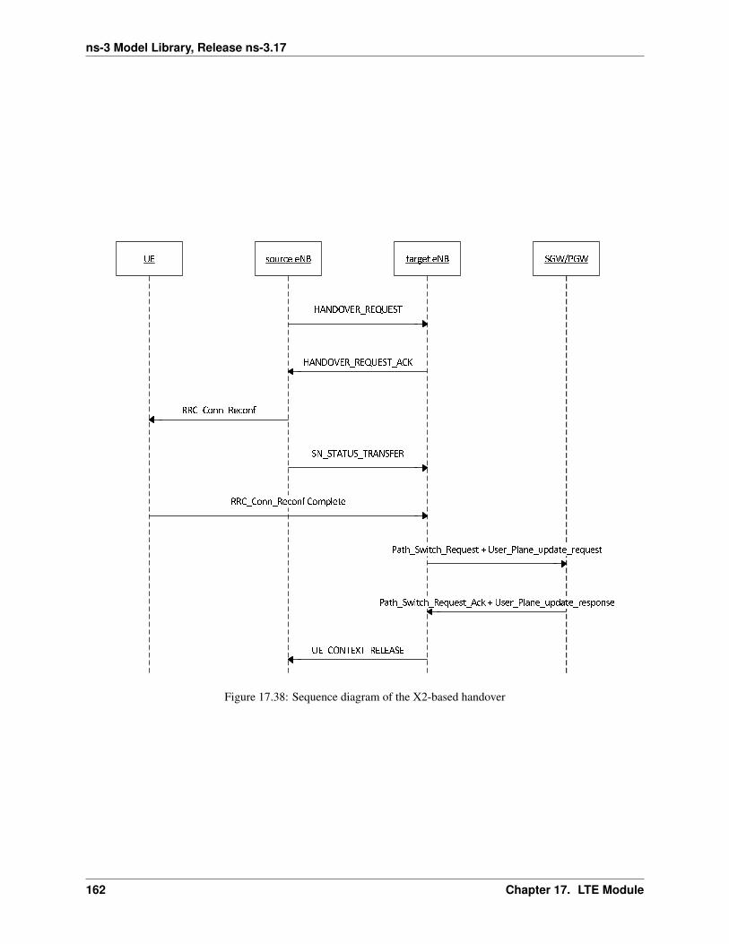
ns-3 Model Library, Release ns-3.17
��������� �������
���������������
�������������������
������������������
������������������
�� ��� !��
������""�����"#
!�$��%&�$���'����(������!)�"���*+�����'���
!�$��%&�$���'������,�(������!)�"���*+������*�"��
������""�����"#���-*)��
Figure 17.38: Sequence diagram of the X2-based handover
162 Chapter 17. LTE Module
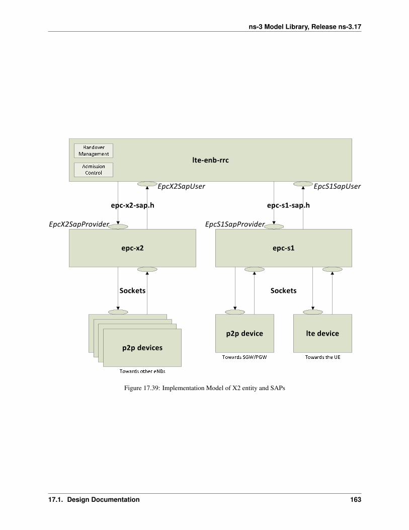
ns-3 Model Library, Release ns-3.17
�����������
����
����������
���������� ����
������ ��
��������
�����
�������
����������
���������� ����
������� ��
��������� ��
����
��������
�������
��������� ��
����
��������
��������� ��
����
�����������������
�������������� �
���������������
����������
������������
���������
������
��������
���������
Figure 17.39: Implementation Model of X2 entity and SAPs
17.1. Design Documentation 163
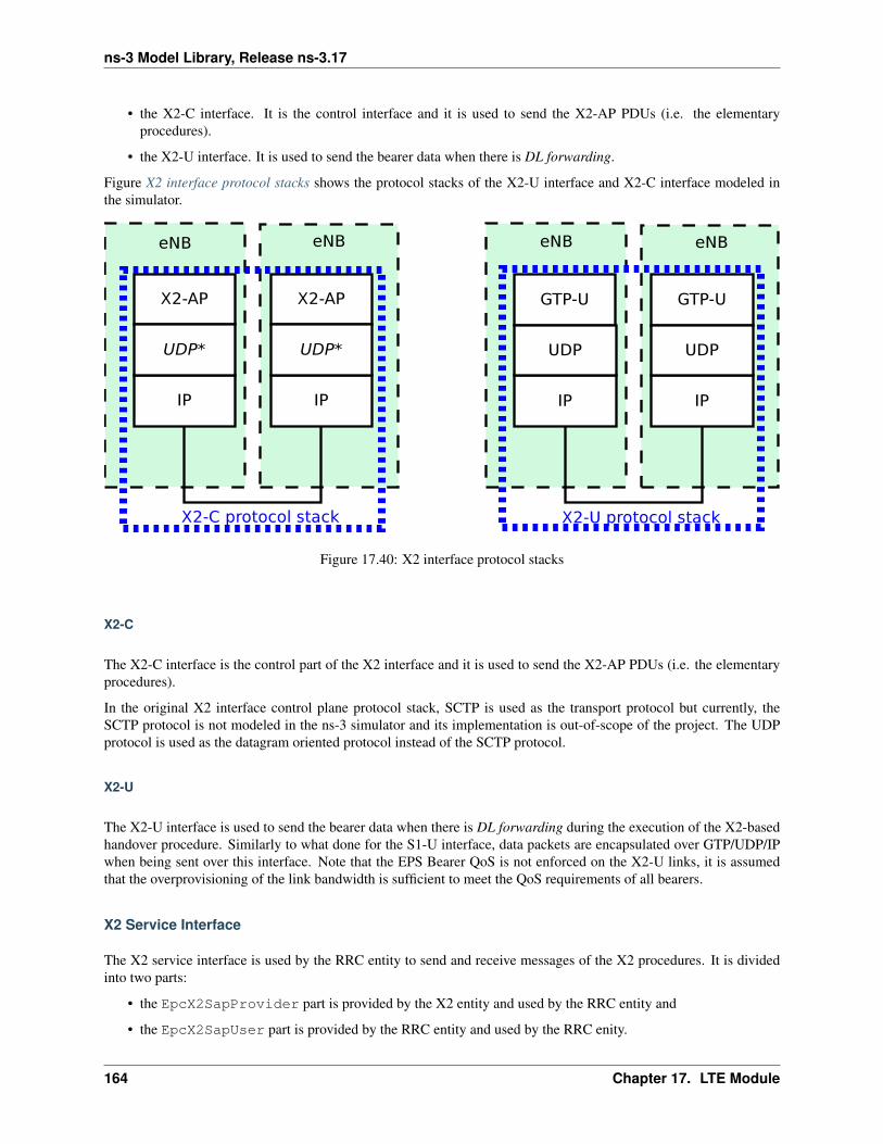
ns-3 Model Library, Release ns-3.17
• the X2-C interface. It is the control interface and it is used to send the X2-AP PDUs (i.e. the elementaryprocedures).
• the X2-U interface. It is used to send the bearer data when there is DL forwarding.
Figure X2 interface protocol stacks shows the protocol stacks of the X2-U interface and X2-C interface modeled inthe simulator.
Figure 17.40: X2 interface protocol stacks
X2-C
The X2-C interface is the control part of the X2 interface and it is used to send the X2-AP PDUs (i.e. the elementaryprocedures).
In the original X2 interface control plane protocol stack, SCTP is used as the transport protocol but currently, theSCTP protocol is not modeled in the ns-3 simulator and its implementation is out-of-scope of the project. The UDPprotocol is used as the datagram oriented protocol instead of the SCTP protocol.
X2-U
The X2-U interface is used to send the bearer data when there is DL forwarding during the execution of the X2-basedhandover procedure. Similarly to what done for the S1-U interface, data packets are encapsulated over GTP/UDP/IPwhen being sent over this interface. Note that the EPS Bearer QoS is not enforced on the X2-U links, it is assumedthat the overprovisioning of the link bandwidth is sufficient to meet the QoS requirements of all bearers.
X2 Service Interface
The X2 service interface is used by the RRC entity to send and receive messages of the X2 procedures. It is dividedinto two parts:
• the EpcX2SapProvider part is provided by the X2 entity and used by the RRC entity and
• the EpcX2SapUser part is provided by the RRC entity and used by the RRC enity.
164 Chapter 17. LTE Module
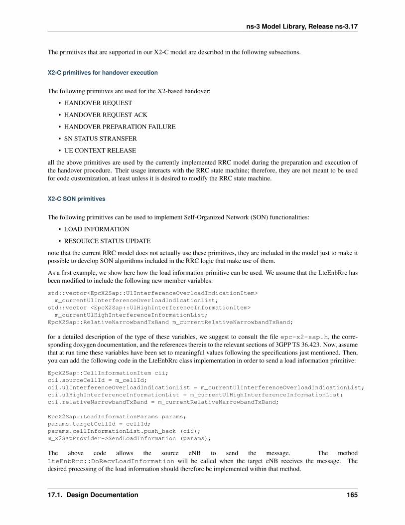
ns-3 Model Library, Release ns-3.17
The primitives that are supported in our X2-C model are described in the following subsections.
X2-C primitives for handover execution
The following primitives are used for the X2-based handover:
• HANDOVER REQUEST
• HANDOVER REQUEST ACK
• HANDOVER PREPARATION FAILURE
• SN STATUS STRANSFER
• UE CONTEXT RELEASE
all the above primitives are used by the currently implemented RRC model during the preparation and execution ofthe handover procedure. Their usage interacts with the RRC state machine; therefore, they are not meant to be usedfor code customization, at least unless it is desired to modify the RRC state machine.
X2-C SON primitives
The following primitives can be used to implement Self-Organized Network (SON) functionalities:
• LOAD INFORMATION
• RESOURCE STATUS UPDATE
note that the current RRC model does not actually use these primitives, they are included in the model just to make itpossible to develop SON algorithms included in the RRC logic that make use of them.
As a first example, we show here how the load information primitive can be used. We assume that the LteEnbRrc hasbeen modified to include the following new member variables:
std::vector<EpcX2Sap::UlInterferenceOverloadIndicationItem>m_currentUlInterferenceOverloadIndicationList;
std::vector <EpcX2Sap::UlHighInterferenceInformationItem>m_currentUlHighInterferenceInformationList;
EpcX2Sap::RelativeNarrowbandTxBand m_currentRelativeNarrowbandTxBand;
for a detailed description of the type of these variables, we suggest to consult the file epc-x2-sap.h, the corre-sponding doxygen documentation, and the references therein to the relevant sections of 3GPP TS 36.423. Now, assumethat at run time these variables have been set to meaningful values following the specifications just mentioned. Then,you can add the following code in the LteEnbRrc class implementation in order to send a load information primitive:
EpcX2Sap::CellInformationItem cii;cii.sourceCellId = m_cellId;cii.ulInterferenceOverloadIndicationList = m_currentUlInterferenceOverloadIndicationList;cii.ulHighInterferenceInformationList = m_currentUlHighInterferenceInformationList;cii.relativeNarrowbandTxBand = m_currentRelativeNarrowbandTxBand;
EpcX2Sap::LoadInformationParams params;params.targetCellId = cellId;params.cellInformationList.push_back (cii);m_x2SapProvider->SendLoadInformation (params);
The above code allows the source eNB to send the message. The methodLteEnbRrc::DoRecvLoadInformation will be called when the target eNB receives the message. Thedesired processing of the load information should therefore be implemented within that method.
17.1. Design Documentation 165
ns-3 Model Library, Release ns-3.17
In the following second example we show how the resource status update primitive is used. We assume that theLteEnbRrc has been modified to include the following new member variable:
EpcX2Sap::CellMeasurementResultItem m_cmri;
similarly to before, we refer to epc-x2-sap.h and the references therein for detailed information about this variabletype. Again, we assume that the variable has been already set to a meaningful value. Then, you can add the followingcode in order to send a resource status update:
EpcX2Sap::ResourceStatusUpdateParams params;params.targetCellId = cellId;params.cellMeasurementResultList.push_back (m_cmri);m_x2SapProvider->SendResourceStatusUpdate (params);
The method eEnbRrc::DoRecvResourceStatusUpdate will be called when the target eNB receives the re-source status update message. The desired processing of this message should therefore be implemented within thatmethod.
Finally, we note that the setting and processing of the appropriate values for the variable passed to the above de-scribed primitives is deemed to be specific of the SON algorithm being implemented, and hence is not covered by thisdocumentation.
Unsupported primitives
Mobility Robustness Optimization primitives such as Radio Link Failure indication and Handover Report are notsupported at this stage.
166 Chapter 17. LTE Module

ns-3 Model Library, Release ns-3.17
17.1.14 S11
The S11 interface provides control plane interaction between the SGW and the MME using the GTPv2-C protocolspecified in [TS29274]. In the simulator, this interface is modeled in an ideal fashion, with direct interaction betweenthe SGW and the MME objects, without actually implementing the encoding of the messages and without actuallytransmitting any PDU on any link.
The S11 primitives that are modeled are:
• CREATE SESSION REQUEST
• CREATE SESSION RESPONSE
• MODIFY BEARER REQUEST
• MODIFY BEARER RESPONSE
Of these primitives, the first two are used upon initial UE attachment for the establishment of the S1-U bearers; theother two are used during handover to switch the S1-U bearers from the source eNB to the target eNB as a consequenceof the reception by the MME of a PATH SWITCH REQUEST S1-AP message.
17.1. Design Documentation 167
ns-3 Model Library, Release ns-3.17
17.1.15 Helpers
Two helper objects are use to setup simulations and configure the various components. These objects are:
• LteHelper, which takes care of the configuration of the LTE radio access network, as well as of coordinating thesetup and release of EPS bearers
• EpcHelper, which takes care of the configuratio of the Evolved Packet Core
It is possible to create a simple LTE-only simulations by using LteHelper alone, or to create complete LTE-EPCsimulations by using both LteHelper and EpcHelper. When both helpers are used, they interact in a master-slavefashion, with LteHelper being the Master that interacts directly with the user program, and EpcHelper working “underthe hood” to configure the EPC upon explicit methods called by LteHelper. The exact interactions are displayed in theFigure Sequence diagram of the interaction between LteHelper and EpcHelper.
17.2 User Documentation
17.2.1 Background
We assume the reader is already familiar with how to use the ns-3 simulator to run generic simulation programs. Ifthis is not the case, we strongly recommend the reader to consult [ns3tutorial].
17.2.2 Usage Overview
The ns-3 LTE model is a software library that allows the simulation of LTE networks, optionally including the EvolvedPacket Core (EPC). The process of performing such simulations typically involves the following steps:
1. Define the scenario to be simulated
2. Write a simulation program that recreates the desired scenario topology/architecture. This is done accessing thens-3 LTE model library using the ns3::LteHelper API defined in src/lte/helper/lte-helper.h.
3. Specify configuration parameters of the objects that are being used for the simulation. This can be done usinginput files (via the ns3::ConfigStore) or directly within the simulation program.
4. Configure the desired output to be produced by the simulator
5. Run the simulation.
All these aspects will be explained in the following sections by means of practical examples.
17.2.3 Basic simulation program
Here is the minimal simulation program that is needed to do an LTE-only simulation (without EPC).
1. Initial boilerplate:
#include <ns3/core-module.h>#include <ns3/network-module.h>#include <ns3/mobility-module.h>#include <ns3/lte-module.h>
using namespace ns3;
int main (int argc, char *argv[])
168 Chapter 17. LTE Module
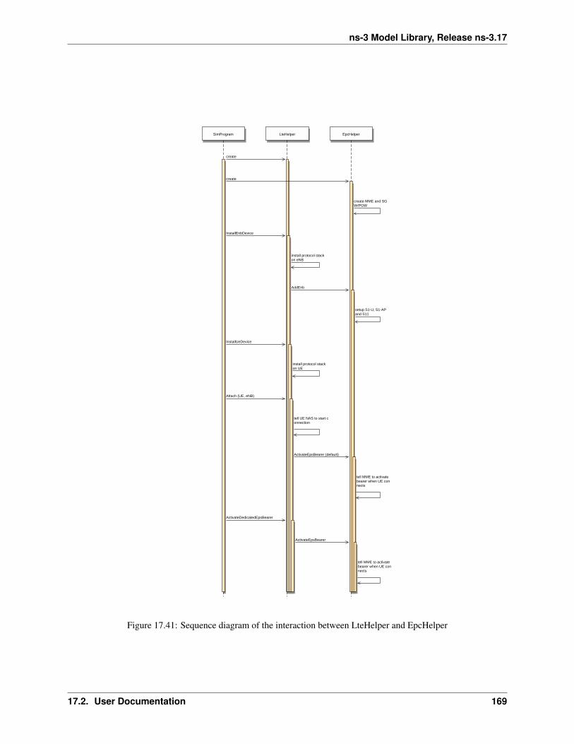
ns-3 Model Library, Release ns-3.17
SimProgram LteHelper EpcHelper
create
create
create MME and SGW/PGW
InstallEnbDevice
install protocol stack on eNB
AddEnb
setup S1-U, S1-AP and S11
InstallUeDevice
install protocol stack on UE
Attach (UE, eNB)
tell UE NAS to start connection
ActivateEpsBearer (default)
tell MME to activate bearer when UE connects
ActivateDedicatedEpsBearer
ActivateEpsBearer
tell MME to activate bearer when UE connects
Figure 17.41: Sequence diagram of the interaction between LteHelper and EpcHelper
17.2. User Documentation 169

ns-3 Model Library, Release ns-3.17
{// the rest of the simulation program follows
2. Create a LteHelper object:
Ptr<LteHelper> lteHelper = CreateObject<LteHelper> ();
This will instantiate some common objects (e.g., the Channel object) and provide the methods to add eNBs andUEs and configure them.
3. Create Node objects for the eNB(s) and the UEs:
NodeContainer enbNodes;enbNodes.Create (1);NodeContainer ueNodes;ueNodes.Create (2);
Note that the above Node instances at this point still don’t have an LTE protocol stack installed; they’re justempty nodes.
4. Configure the Mobility model for all the nodes:
MobilityHelper mobility;mobility.SetMobilityModel ("ns3::ConstantPositionMobilityModel");mobility.Install (enbNodes);mobility.SetMobilityModel ("ns3::ConstantPositionMobilityModel");mobility.Install (ueNodes);
The above will place all nodes at the coordinates (0,0,0). Please refer to the documentation of the ns-3 mobilitymodel for how to set your own position or configure node movement.
5. Install an LTE protocol stack on the eNB(s):
NetDeviceContainer enbDevs;enbDevs = lteHelper->InstallEnbDevice (enbNodes);
6. Install an LTE protocol stack on the UEs:
NetDeviceContainer ueDevs;ueDevs = lteHelper->InstallUeDevice (ueNodes);
7. Attach the UEs to an eNB. This will configure each UE according to the eNB configuration, and create an RRCconnection between them:
lteHelper->Attach (ueDevs, enbDevs.Get (0));
8. Activate a data radio bearer between each UE and the eNB it is attached to:
enum EpsBearer::Qci q = EpsBearer::GBR_CONV_VOICE;EpsBearer bearer (q);lteHelper->ActivateDataRadioBearer (ueDevs, bearer);
this method will also activate two saturation traffic generators for that bearer, one in uplink and one in downlink.
9. Set the stop time:
Simulator::Stop (Seconds (0.005));
This is needed otherwise the simulation will last forever, because (among others) the start-of-subframe event isscheduled repeatedly, and the ns-3 simulator scheduler will hence never run out of events.
10. Run the simulation:
170 Chapter 17. LTE Module
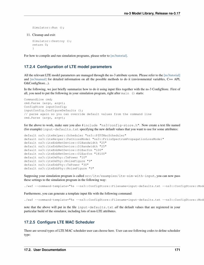
ns-3 Model Library, Release ns-3.17
Simulator::Run ();
11. Cleanup and exit:
Simulator::Destroy ();return 0;}
For how to compile and run simulation programs, please refer to [ns3tutorial].
17.2.4 Configuration of LTE model parameters
All the relevant LTE model parameters are managed through the ns-3 attribute system. Please refer to the [ns3tutorial]and [ns3manual] for detailed information on all the possible methods to do it (environmental variables, C++ API,GtkConfigStore...).
In the following, we just briefly summarize how to do it using input files together with the ns-3 ConfigStore. First ofall, you need to put the following in your simulation program, right after main () starts:
CommandLine cmd;cmd.Parse (argc, argv);ConfigStore inputConfig;inputConfig.ConfigureDefaults ();// parse again so you can override default values from the command linecmd.Parse (argc, argv);
for the above to work, make sure you also #include "ns3/config-store.h". Now create a text file named(for example) input-defaults.txt specifying the new default values that you want to use for some attributes:
default ns3::LteHelper::Scheduler "ns3::PfFfMacScheduler"default ns3::LteHelper::PathlossModel "ns3::FriisSpectrumPropagationLossModel"default ns3::LteEnbNetDevice::UlBandwidth "25"default ns3::LteEnbNetDevice::DlBandwidth "25"default ns3::LteEnbNetDevice::DlEarfcn "100"default ns3::LteEnbNetDevice::UlEarfcn "18100"default ns3::LteUePhy::TxPower "10"default ns3::LteUePhy::NoiseFigure "9"default ns3::LteEnbPhy::TxPower "30"default ns3::LteEnbPhy::NoiseFigure "5"
Supposing your simulation program is called src/lte/examples/lte-sim-with-input, you can now passthese settings to the simulation program in the following way:
./waf --command-template="%s --ns3::ConfigStore::Filename=input-defaults.txt --ns3::ConfigStore::Mode=Load --ns3::ConfigStore::FileFormat=RawText" --run src/lte/examples/lte-sim-with-input
Furthermore, you can generate a template input file with the following command:
./waf --command-template="%s --ns3::ConfigStore::Filename=input-defaults.txt --ns3::ConfigStore::Mode=Save --ns3::ConfigStore::FileFormat=RawText" --run src/lte/examples/lte-sim-with-input
note that the above will put in the file input-defaults.txt all the default values that are registered in yourparticular build of the simulator, including lots of non-LTE attributes.
17.2.5 Configure LTE MAC Scheduler
There are several types of LTE MAC scheduler user can choose here. User can use following codes to define schedulertype:
17.2. User Documentation 171
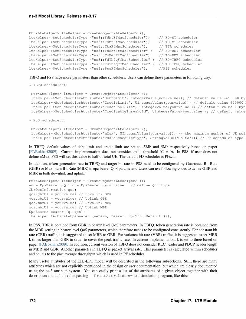
ns-3 Model Library, Release ns-3.17
Ptr<LteHelper> lteHelper = CreateObject<LteHelper> ();lteHelper->SetSchedulerType ("ns3::FdMtFfMacScheduler"); // FD-MT schedulerlteHelper->SetSchedulerType ("ns3::TdMtFfMacScheduler"); // TD-MT schedulerlteHelper->SetSchedulerType ("ns3::TtaFfMacScheduler"); // TTA schedulerlteHelper->SetSchedulerType ("ns3::FdBetFfMacScheduler"); // FD-BET schedulerlteHelper->SetSchedulerType ("ns3::TdBetFfMacScheduler"); // TD-BET schedulerlteHelper->SetSchedulerType ("ns3::FdTbfqFfMacScheduler"); // FD-TBFQ schedulerlteHelper->SetSchedulerType ("ns3::TdTbfqFfMacScheduler"); // TD-TBFQ schedulerlteHelper->SetSchedulerType ("ns3::PssFfMacScheduler"); //PSS scheduler
TBFQ and PSS have more parameters than other schedulers. Users can define those parameters in following way:
* TBFQ scheduler::
Ptr<LteHelper> lteHelper = CreateObject<LteHelper> ();lteHelper->SetSchedulerAttribute("DebtLimit", IntegerValue(yourvalue)); // default value -625000 bytes (-5Mb)lteHelper->SetSchedulerAttribute("CreditLimit", UintegerValue(yourvalue)); // default value 625000 bytes (5Mb)lteHelper->SetSchedulerAttribute("TokenPoolSize", UintegerValue(yourvalue)); // default value 1 bytelteHelper->SetSchedulerAttribute("CreditableThreshold", UintegerValue(yourvalue)); // default value 0
* PSS scheduler::
Ptr<LteHelper> lteHelper = CreateObject<LteHelper> ();lteHelper->SetSchedulerAttribute("nMux", UIntegerValue(yourvalue)); // the maximum number of UE selected by TD schedulerlteHelper->SetSchedulerAttribute("PssFdSchedulerType", StringValue("CoItA")); // PF scheduler type in PSS
In TBFQ, default values of debt limit and credit limit are set to -5Mb and 5Mb respectively based on paper[FABokhari2009]. Current implementation does not consider credit threshold (C = 0). In PSS, if user does notdefine nMux, PSS will set this value to half of total UE. The default FD scheduler is PFsch.
In addition, token generation rate in TBFQ and target bit rate in PSS need to be configured by Guarantee Bit Rate(GBR) or Maximum Bit Rate (MBR) in epc bearer QoS parameters. Users can use following codes to define GBR andMBR in both downlink and uplink:
Ptr<LteHelper> lteHelper = CreateObject<LteHelper> ();enum EpsBearer::Qci q = EpsBearer::yourvalue; // define Qci typeGbrQosInformation qos;qos.gbrDl = yourvalue; // Downlink GBRqos.gbrUl = yourvalue; // Uplink GBRqos.mbrDl = yourvalue; // Downlink MBRqos.mbrUl = yourvalue; // Uplink MBREpsBearer bearer (q, qos);lteHelper->ActivateEpsBearer (ueDevs, bearer, EpcTft::Default ());
In PSS, TBR is obtained from GBR in bearer level QoS parameters. In TBFQ, token generation rate is obtained fromthe MBR setting in bearer level QoS parameters, which therefore needs to be configured consistently. For constant bitrate (CBR) traffic, it is suggested to set MBR to GBR. For variance bit rate (VBR) traffic, it is suggested to set MBRk times larger than GBR in order to cover the peak traffic rate. In current implementation, k is set to three based onpaper [FABokhari2009]. In addition, current version of TBFQ does not consider RLC header and PDCP header lengthin MBR and GBR. Another parameter in TBFQ is packet arrival rate. This parameter is calculated within schedulerand equals to the past average throughput which is used in PF scheduler.
Many useful attributes of the LTE-EPC model will be described in the following subsections. Still, there are manyattributes which are not explicitly mentioned in the design or user documentation, but which are clearly documentedusing the ns-3 attribute system. You can easily print a list of the attributes of a given object together with theirdescription and default value passing --PrintAttributes= to a simulation program, like this:
172 Chapter 17. LTE Module
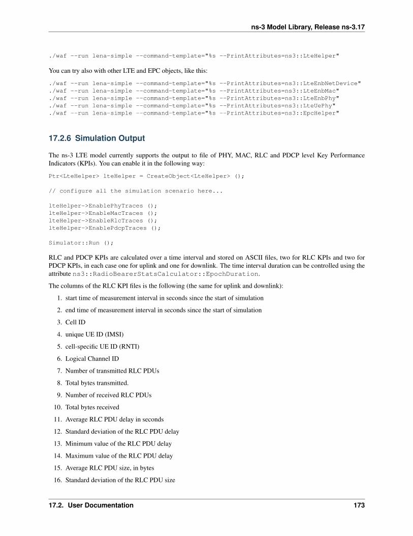
ns-3 Model Library, Release ns-3.17
./waf --run lena-simple --command-template="%s --PrintAttributes=ns3::LteHelper"
You can try also with other LTE and EPC objects, like this:
./waf --run lena-simple --command-template="%s --PrintAttributes=ns3::LteEnbNetDevice"
./waf --run lena-simple --command-template="%s --PrintAttributes=ns3::LteEnbMac"
./waf --run lena-simple --command-template="%s --PrintAttributes=ns3::LteEnbPhy"
./waf --run lena-simple --command-template="%s --PrintAttributes=ns3::LteUePhy"
./waf --run lena-simple --command-template="%s --PrintAttributes=ns3::EpcHelper"
17.2.6 Simulation Output
The ns-3 LTE model currently supports the output to file of PHY, MAC, RLC and PDCP level Key PerformanceIndicators (KPIs). You can enable it in the following way:
Ptr<LteHelper> lteHelper = CreateObject<LteHelper> ();
// configure all the simulation scenario here...
lteHelper->EnablePhyTraces ();lteHelper->EnableMacTraces ();lteHelper->EnableRlcTraces ();lteHelper->EnablePdcpTraces ();
Simulator::Run ();
RLC and PDCP KPIs are calculated over a time interval and stored on ASCII files, two for RLC KPIs and two forPDCP KPIs, in each case one for uplink and one for downlink. The time interval duration can be controlled using theattribute ns3::RadioBearerStatsCalculator::EpochDuration.
The columns of the RLC KPI files is the following (the same for uplink and downlink):
1. start time of measurement interval in seconds since the start of simulation
2. end time of measurement interval in seconds since the start of simulation
3. Cell ID
4. unique UE ID (IMSI)
5. cell-specific UE ID (RNTI)
6. Logical Channel ID
7. Number of transmitted RLC PDUs
8. Total bytes transmitted.
9. Number of received RLC PDUs
10. Total bytes received
11. Average RLC PDU delay in seconds
12. Standard deviation of the RLC PDU delay
13. Minimum value of the RLC PDU delay
14. Maximum value of the RLC PDU delay
15. Average RLC PDU size, in bytes
16. Standard deviation of the RLC PDU size
17.2. User Documentation 173

ns-3 Model Library, Release ns-3.17
17. Minimum RLC PDU size
18. Maximum RLC PDU size
Similarly, the columns of the PDCP KPI files is the following (again, the same for uplink and downlink):
1. start time of measurement interval in seconds since the start of simulation
2. end time of measurement interval in seconds since the start of simulation
3. Cell ID
4. unique UE ID (IMSI)
5. cell-specific UE ID (RNTI)
6. Logical Channel ID
7. Number of transmitted PDCP PDUs
8. Total bytes transmitted.
9. Number of received PDCP PDUs
10. Total bytes received
11. Average PDCP PDU delay in seconds
12. Standard deviation of the PDCP PDU delay
13. Minimum value of the PDCP PDU delay
14. Maximum value of the PDCP PDU delay
15. Average PDCP PDU size, in bytes
16. Standard deviation of the PDCP PDU size
17. Minimum PDCP PDU size
18. Maximum PDCP PDU size
MAC KPIs are basically a trace of the resource allocation reported by the scheduler upon the start of every subframe.They are stored in ASCII files. For downlink MAC KPIs the format is the following:
1. Simulation time in seconds at which the allocation is indicated by the scheduler
2. Cell ID
3. unique UE ID (IMSI)
4. Frame number
5. Subframe number
6. cell-specific UE ID (RNTI)
7. MCS of TB 1
8. size of TB 1
9. MCS of TB 2 (0 if not present)
10. size of TB 2 (0 if not present)
while for uplink MAC KPIs the format is:
1. Simulation time in seconds at which the allocation is indicated by the scheduler
2. Cell ID
174 Chapter 17. LTE Module
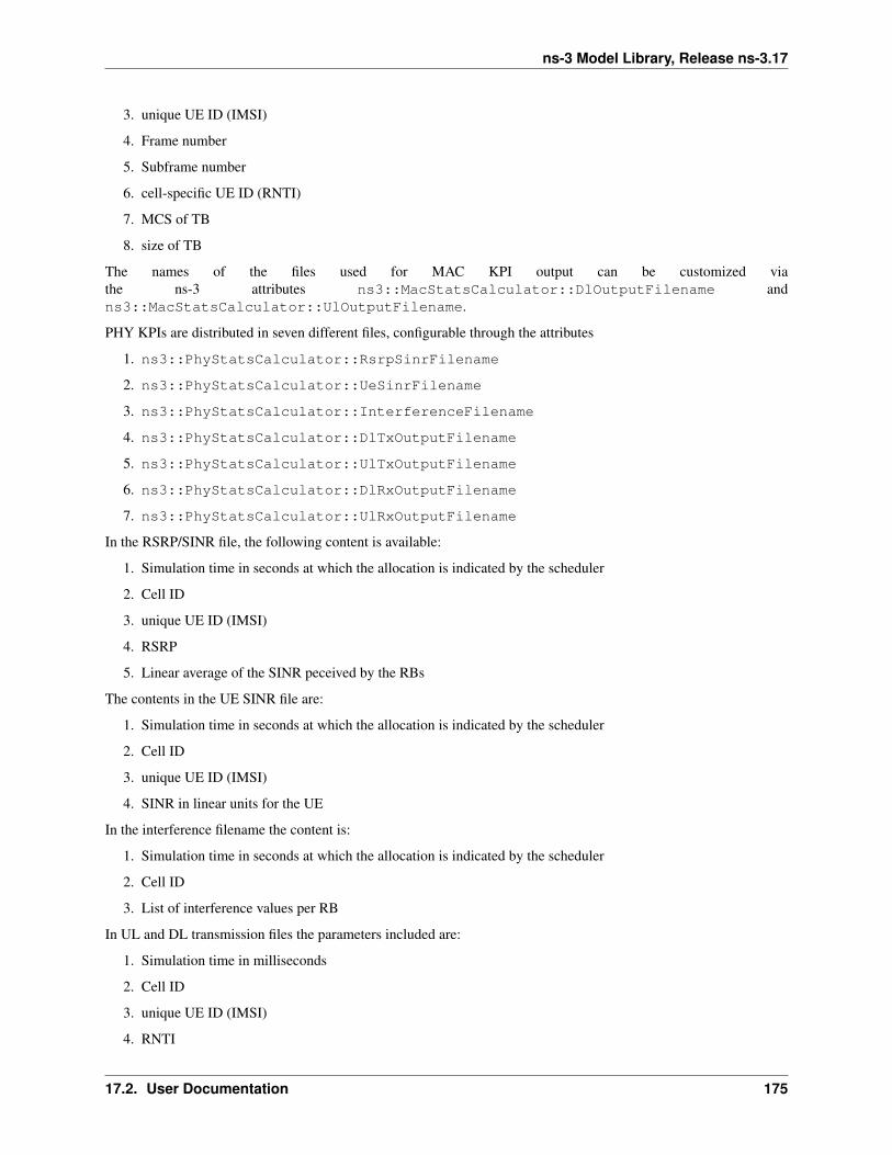
ns-3 Model Library, Release ns-3.17
3. unique UE ID (IMSI)
4. Frame number
5. Subframe number
6. cell-specific UE ID (RNTI)
7. MCS of TB
8. size of TB
The names of the files used for MAC KPI output can be customized viathe ns-3 attributes ns3::MacStatsCalculator::DlOutputFilename andns3::MacStatsCalculator::UlOutputFilename.
PHY KPIs are distributed in seven different files, configurable through the attributes
1. ns3::PhyStatsCalculator::RsrpSinrFilename
2. ns3::PhyStatsCalculator::UeSinrFilename
3. ns3::PhyStatsCalculator::InterferenceFilename
4. ns3::PhyStatsCalculator::DlTxOutputFilename
5. ns3::PhyStatsCalculator::UlTxOutputFilename
6. ns3::PhyStatsCalculator::DlRxOutputFilename
7. ns3::PhyStatsCalculator::UlRxOutputFilename
In the RSRP/SINR file, the following content is available:
1. Simulation time in seconds at which the allocation is indicated by the scheduler
2. Cell ID
3. unique UE ID (IMSI)
4. RSRP
5. Linear average of the SINR peceived by the RBs
The contents in the UE SINR file are:
1. Simulation time in seconds at which the allocation is indicated by the scheduler
2. Cell ID
3. unique UE ID (IMSI)
4. SINR in linear units for the UE
In the interference filename the content is:
1. Simulation time in seconds at which the allocation is indicated by the scheduler
2. Cell ID
3. List of interference values per RB
In UL and DL transmission files the parameters included are:
1. Simulation time in milliseconds
2. Cell ID
3. unique UE ID (IMSI)
4. RNTI
17.2. User Documentation 175
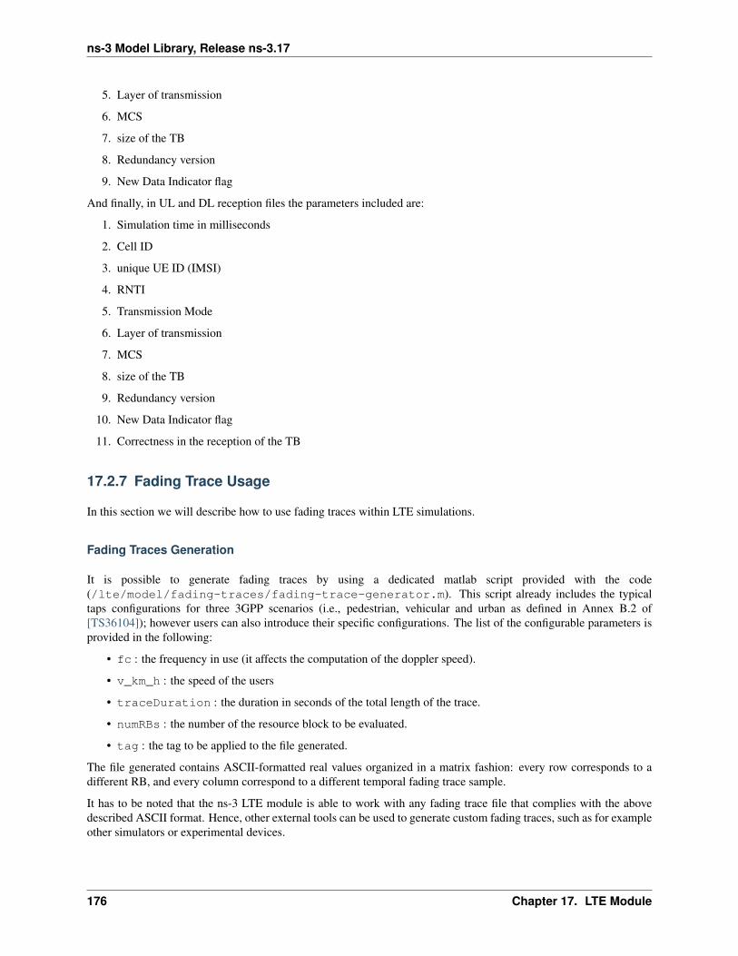
ns-3 Model Library, Release ns-3.17
5. Layer of transmission
6. MCS
7. size of the TB
8. Redundancy version
9. New Data Indicator flag
And finally, in UL and DL reception files the parameters included are:
1. Simulation time in milliseconds
2. Cell ID
3. unique UE ID (IMSI)
4. RNTI
5. Transmission Mode
6. Layer of transmission
7. MCS
8. size of the TB
9. Redundancy version
10. New Data Indicator flag
11. Correctness in the reception of the TB
17.2.7 Fading Trace Usage
In this section we will describe how to use fading traces within LTE simulations.
Fading Traces Generation
It is possible to generate fading traces by using a dedicated matlab script provided with the code(/lte/model/fading-traces/fading-trace-generator.m). This script already includes the typicaltaps configurations for three 3GPP scenarios (i.e., pedestrian, vehicular and urban as defined in Annex B.2 of[TS36104]); however users can also introduce their specific configurations. The list of the configurable parameters isprovided in the following:
• fc : the frequency in use (it affects the computation of the doppler speed).
• v_km_h : the speed of the users
• traceDuration : the duration in seconds of the total length of the trace.
• numRBs : the number of the resource block to be evaluated.
• tag : the tag to be applied to the file generated.
The file generated contains ASCII-formatted real values organized in a matrix fashion: every row corresponds to adifferent RB, and every column correspond to a different temporal fading trace sample.
It has to be noted that the ns-3 LTE module is able to work with any fading trace file that complies with the abovedescribed ASCII format. Hence, other external tools can be used to generate custom fading traces, such as for exampleother simulators or experimental devices.
176 Chapter 17. LTE Module
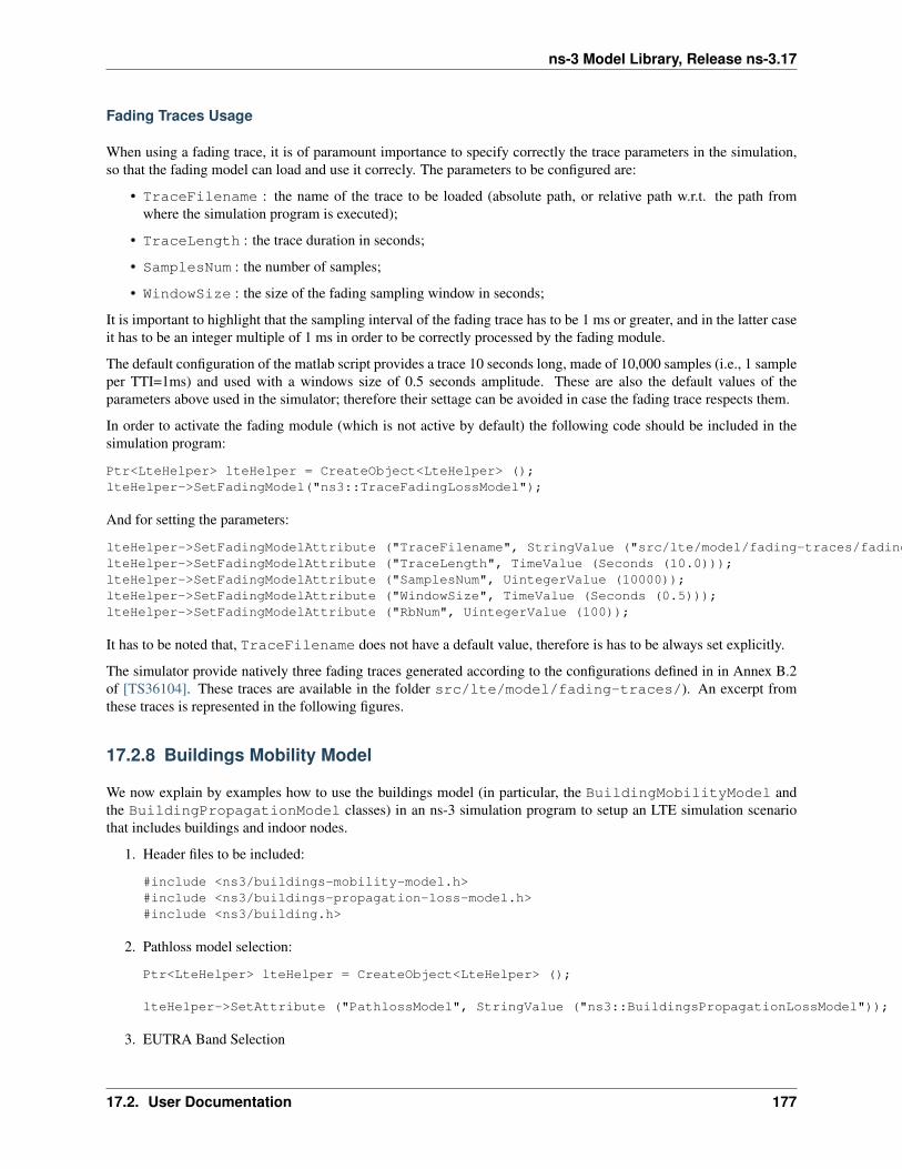
ns-3 Model Library, Release ns-3.17
Fading Traces Usage
When using a fading trace, it is of paramount importance to specify correctly the trace parameters in the simulation,so that the fading model can load and use it correcly. The parameters to be configured are:
• TraceFilename : the name of the trace to be loaded (absolute path, or relative path w.r.t. the path fromwhere the simulation program is executed);
• TraceLength : the trace duration in seconds;
• SamplesNum : the number of samples;
• WindowSize : the size of the fading sampling window in seconds;
It is important to highlight that the sampling interval of the fading trace has to be 1 ms or greater, and in the latter caseit has to be an integer multiple of 1 ms in order to be correctly processed by the fading module.
The default configuration of the matlab script provides a trace 10 seconds long, made of 10,000 samples (i.e., 1 sampleper TTI=1ms) and used with a windows size of 0.5 seconds amplitude. These are also the default values of theparameters above used in the simulator; therefore their settage can be avoided in case the fading trace respects them.
In order to activate the fading module (which is not active by default) the following code should be included in thesimulation program:
Ptr<LteHelper> lteHelper = CreateObject<LteHelper> ();lteHelper->SetFadingModel("ns3::TraceFadingLossModel");
And for setting the parameters:
lteHelper->SetFadingModelAttribute ("TraceFilename", StringValue ("src/lte/model/fading-traces/fading_trace_EPA_3kmph.fad"));lteHelper->SetFadingModelAttribute ("TraceLength", TimeValue (Seconds (10.0)));lteHelper->SetFadingModelAttribute ("SamplesNum", UintegerValue (10000));lteHelper->SetFadingModelAttribute ("WindowSize", TimeValue (Seconds (0.5)));lteHelper->SetFadingModelAttribute ("RbNum", UintegerValue (100));
It has to be noted that, TraceFilename does not have a default value, therefore is has to be always set explicitly.
The simulator provide natively three fading traces generated according to the configurations defined in in Annex B.2of [TS36104]. These traces are available in the folder src/lte/model/fading-traces/). An excerpt fromthese traces is represented in the following figures.
17.2.8 Buildings Mobility Model
We now explain by examples how to use the buildings model (in particular, the BuildingMobilityModel andthe BuildingPropagationModel classes) in an ns-3 simulation program to setup an LTE simulation scenariothat includes buildings and indoor nodes.
1. Header files to be included:
#include <ns3/buildings-mobility-model.h>#include <ns3/buildings-propagation-loss-model.h>#include <ns3/building.h>
2. Pathloss model selection:
Ptr<LteHelper> lteHelper = CreateObject<LteHelper> ();
lteHelper->SetAttribute ("PathlossModel", StringValue ("ns3::BuildingsPropagationLossModel"));
3. EUTRA Band Selection
17.2. User Documentation 177
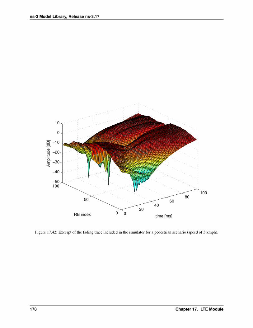
ns-3 Model Library, Release ns-3.17
020
4060
80100
0
50
100−50
−40
−30
−20
−10
0
10
time [ms]RB index
Am
plit
ude [dB
]
Figure 17.42: Excerpt of the fading trace included in the simulator for a pedestrian scenario (speed of 3 kmph).
178 Chapter 17. LTE Module
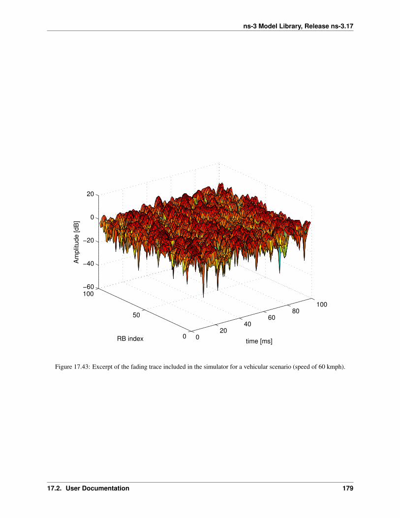
ns-3 Model Library, Release ns-3.17
020
4060
80100
0
50
100−60
−40
−20
0
20
time [ms]RB index
Am
plit
ude [dB
]
Figure 17.43: Excerpt of the fading trace included in the simulator for a vehicular scenario (speed of 60 kmph).
17.2. User Documentation 179
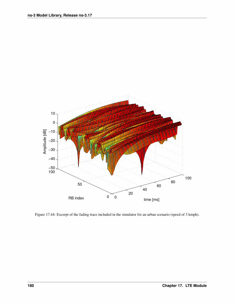
ns-3 Model Library, Release ns-3.17
020
4060
80100
0
50
100−50
−40
−30
−20
−10
0
10
time [ms]RB index
Am
plit
ude [dB
]
Figure 17.44: Excerpt of the fading trace included in the simulator for an urban scenario (speed of 3 kmph).
180 Chapter 17. LTE Module
ns-3 Model Library, Release ns-3.17
The selection of the working frequency of the propagation model has to be done with the standard ns-3 attributesystem as described in the correspond section (“Configuration of LTE model parameters”) by means of the DlEarfcnand UlEarfcn parameters, for instance:
lteHelper->SetEnbDeviceAttribute ("DlEarfcn", UintegerValue (100));lteHelper->SetEnbDeviceAttribute ("UlEarfcn", UintegerValue (18100));
It is to be noted that using other means to configure the frequency used by the propagation model (i.e., configuringthe corresponding BuildingsPropagationLossModel attributes directly) might generates conflicts in the frequenciesdefinition in the modules during the simulation, and is therefore not advised.
1. Mobility model selection:
MobilityHelper mobility;mobility.SetMobilityModel ("ns3::BuildingsMobilityModel");
2. Building creation:
double x_min = 0.0;double x_max = 10.0;double y_min = 0.0;double y_max = 20.0;double z_min = 0.0;double z_max = 10.0;Ptr<Building> b = CreateObject <Building> ();b->SetBoundaries (Box (x_min, x_max, y_min, y_max, z_min, z_max));b->SetBuildingType (Building::Residential);b->SetExtWallsType (Building::ConcreteWithWindows);b->SetNFloors (3);b->SetNRoomsX (3);b->SetNRoomsY (2);
This will instantiate a residential building with base of 10 x 20 meters and height of 10 meters whose externalwalls are of concrete with windows; the building has three floors and has an internal 3 x 2 grid of rooms of equalsize.
3. Node creation and positioning:
ueNodes.Create (2);mobility.Install (ueNodes);NetDeviceContainer ueDevs;ueDevs = lteHelper->InstallUeDevice (ueNodes);Ptr<BuildingsMobilityModel> mm0 = enbNodes.Get (0)->GetObject<BuildingsMobilityModel> ();Ptr<BuildingsMobilityModel> mm1 = enbNodes.Get (1)->GetObject<BuildingsMobilityModel> ();mm0->SetPosition (Vector (5.0, 5.0, 1.5));mm1->SetPosition (Vector (30.0, 40.0, 1.5));
This positions the node on the scenario. Note that, in this example, node 0 will be in the building, and node 1 will beout of the building. Note that this alone is not sufficient to setup the topology correctly. What is left to be done is toissue the following command after we have placed all nodes in the simulation:
BuildingsHelper::MakeMobilityModelConsistent ();
This command will go through the lists of all nodes and of all buildings, determine for each user if it is indoor oroutdoor, and if indoor it will also determine the building in which the user is located and the corresponding floor andnumber inside the building.
17.2. User Documentation 181
ns-3 Model Library, Release ns-3.17
17.2.9 PHY Error Model
The Physical error model consists of the data error model and the downlink control error model, both of them activeby default. It is possible to deactivate them with the ns3 attribute system, in detail:
Config::SetDefault ("ns3::LteSpectrumPhy::CtrlErrorModelEnabled", BooleanValue (false));Config::SetDefault ("ns3::LteSpectrumPhy::DataErrorModelEnabled", BooleanValue (false));
17.2.10 MIMO Model
Is this subsection we illustrate how to configure the MIMO parameters. LTE defines 7 types of transmission modes:
• Transmission Mode 1: SISO.
• Transmission Mode 2: MIMO Tx Diversity.
• Transmission Mode 3: MIMO Spatial Multiplexity Open Loop.
• Transmission Mode 4: MIMO Spatial Multiplexity Closed Loop.
• Transmission Mode 5: MIMO Multi-User.
• Transmission Mode 6: Closer loop single layer precoding.
• Transmission Mode 7: Single antenna port 5.
According to model implemented, the simulator includes the first three transmission modes types. The default oneis the Transmission Mode 1 (SISO). In order to change the default Transmission Mode to be used, the attributeDefaultTransmissionMode of the LteEnbRrc can be used, as shown in the following:
Config::SetDefault ("ns3::LteEnbRrc::DefaultTransmissionMode", UintegerValue (0)); // SISOConfig::SetDefault ("ns3::LteEnbRrc::DefaultTransmissionMode", UintegerValue (1)); // MIMO Tx diversity (1 layer)Config::SetDefault ("ns3::LteEnbRrc::DefaultTransmissionMode", UintegerValue (2)); // MIMO Spatial Multiplexity (2 layers)
For changing the transmission mode of a certain user during the simulation a specific interface has been implementedin both standard schedulers:
void TransmissionModeConfigurationUpdate (uint16_t rnti, uint8_t txMode);
This method can be used both for developing transmission mode decision engine (i.e., for optimizing the transmissionmode according to channel condition and/or user’s requirements) and for manual switching from simulation script. Inthe latter case, the switching can be done as shown in the following:
Ptr<LteEnbNetDevice> lteEnbDev = enbDevs.Get (0)->GetObject<LteEnbNetDevice> ();PointerValue ptrval;enbNetDev->GetAttribute ("FfMacScheduler", ptrval);Ptr<RrFfMacScheduler> rrsched = ptrval.Get<RrFfMacScheduler> ();Simulator::Schedule (Seconds (0.2), &RrFfMacScheduler::TransmissionModeConfigurationUpdate, rrsched, rnti, 1);
Finally, the model implemented can be reconfigured according to different MIMO models by updating the gain values(the only constraints is that the gain has to be constant during simulation run-time and common for the layers). Thegain of each Transmission Mode can be changed according to the standard ns3 attribute system, where the attributesare: TxMode1Gain, TxMode2Gain, TxMode3Gain, TxMode4Gain, TxMode5Gain, TxMode6Gain andTxMode7Gain. By default only TxMode1Gain, TxMode2Gain and TxMode3Gain have a meaningful value,that are the ones derived by _[CatreuxMIMO] (i.e., respectively 0.0, 4.2 and -2.8 dB).
182 Chapter 17. LTE Module
ns-3 Model Library, Release ns-3.17
17.2.11 Use of AntennaModel
We now show how associate a particular AntennaModel with an eNB device in order to model a sector of a macroeNB. For this purpose, it is convenient to use the CosineAntennaModel provided by the ns-3 antenna module. Theconfiguration of the eNB is to be done via the LteHelper instance right before the creation of the EnbNetDevice,as shown in the following:
lteHelper->SetEnbAntennaModelType ("ns3::CosineAntennaModel");lteHelper->SetEnbAntennaModelAttribute ("Orientation", DoubleValue (0));lteHelper->SetEnbAntennaModelAttribute ("Beamwidth", DoubleValue (60);lteHelper->SetEnbAntennaModelAttribute ("MaxGain", DoubleValue (0.0));
the above code will generate an antenna model with a 60 degrees beamwidth pointing along the X axis. The orientationis measured in degrees from the X axis, e.g., an orientation of 90 would point along the Y axis, and an orientationof -90 would point in the negative direction along the Y axis. The beamwidth is the -3 dB beamwidth, e.g, for a 60degree beamwidth the antenna gain at an angle of ±30 degrees from the direction of orientation is -3 dB.
To create a multi-sector site, you need to create different ns-3 nodes placed at the same position, and to configureseparate EnbNetDevice with different antenna orientations to be installed on each node.
17.2.12 Radio Environment Maps
By using the class RadioEnvironmentMapHelper it is possible to output to a file a Radio Environment Map (REM),i.e., a uniform 2D grid of values that represent the Signal-to-noise ratio in the downlink with respect to the eNB thathas the strongest signal at each point.
To do this, you just need to add the following code to your simulation program towards the end, right before the callto Simulator::Run ():
Ptr<RadioEnvironmentMapHelper> remHelper = CreateObject<RadioEnvironmentMapHelper> ();remHelper->SetAttribute ("ChannelPath", StringValue ("/ChannelList/0"));remHelper->SetAttribute ("OutputFile", StringValue ("rem.out"));remHelper->SetAttribute ("XMin", DoubleValue (-400.0));remHelper->SetAttribute ("XMax", DoubleValue (400.0));remHelper->SetAttribute ("XRes", UintegerValue (100));remHelper->SetAttribute ("YMin", DoubleValue (-300.0));remHelper->SetAttribute ("YMax", DoubleValue (300.0));remHelper->SetAttribute ("YRes", UintegerValue (75));remHelper->SetAttribute ("Z", DoubleValue (0.0));remHelper->Install ();
By configuring the attributes of the RadioEnvironmentMapHelper object as shown above, you can tune the parametersof the REM to be generated. Note that each RadioEnvironmentMapHelper instance can generate only one REM; ifyou want to generate more REMs, you need to create one separate instance for each REM.
Note that the REM generation is very demanding, in particular:
• the run-time memory consumption is approximately 5KB per pixel. For example, a REM with a resolutionof 500x500 would need about 1.25 GB of memory, and a resolution of 1000x1000 would need needs about5 GB (too much for a regular PC at the time of this writing). To overcome this issue, the REM is generatedat successive steps, with each step evaluating at most a number of pixels determined by the value of the theattribute RadioEnvironmentMapHelper::MaxPointsPerIteration.
• if you generate a REM at the beginning of a simulation, it will slow down the execution of the rest of the simu-lation. If you want to generate a REM for a program and also use the same program to get simulation result, it isrecommended to add a command-line switch that allows to either generate the REM or run the complete simula-tion. For this purpose, note that there is an attribute RadioEnvironmentMapHelper::StopWhenDone(default: true) that will force the simulation to stop right after the REM has been generated.
17.2. User Documentation 183
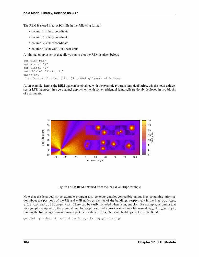
ns-3 Model Library, Release ns-3.17
The REM is stored in an ASCII file in the following format:
• column 1 is the x coordinate
• column 2 is the y coordinate
• column 3 is the z coordinate
• column 4 is the SINR in linear units
A minimal gnuplot script that allows you to plot the REM is given below:
set view map;set xlabel "X"set ylabel "Y"set cblabel "SINR (dB)"unset keyplot "rem.out" using ($1):($2):(10*log10($4)) with image
As an example, here is the REM that can be obtained with the example program lena-dual-stripe, which shows a three-sector LTE macrocell in a co-channel deployment with some residential femtocells randomly deployed in two blocksof apartments.
-10
0
10
20
30
40
50
60
-60 -40 -20 0 20 40 60 80 100
y-co
ordi
nate
(m
)
x-coordinate (m)
-5
0
5
10
15
20
25
30
SIN
R (
dB)
Figure 17.45: REM obtained from the lena-dual-stripe example
Note that the lena-dual-stripe example program also generate gnuplot-compatible output files containing informa-tion about the positions of the UE and eNB nodes as well as of the buildings, respectively in the files ues.txt,enbs.txt and buildings.txt. These can be easily included when using gnuplot. For example, assuming thatyour gnuplot script (e.g., the minimal gnuplot script described above) is saved in a file named my_plot_script,running the following command would plot the location of UEs, eNBs and buildings on top of the REM:
gnuplot -p enbs.txt ues.txt buildings.txt my_plot_script
184 Chapter 17. LTE Module
ns-3 Model Library, Release ns-3.17
17.2.13 AMC Model and CQI Calculation
The simulator provides two possible schemes for what concerns the selection of the MCSs and correspondly thegeneration of the CQIs. The first one is based on the GSoC module [Piro2011] and works per RB basis. This modelcan be activated with the ns3 attribute system, as presented in the following:
Config::SetDefault ("ns3::LteAmc::AmcModel", EnumValue (LteAmc::PiroEW2010));
While, the solution based on the physical error model can be controlled with:
Config::SetDefault ("ns3::LteAmc::AmcModel", EnumValue (LteAmc::MiErrorModel));
Finally, the required efficiency of the PiroEW2010 AMC module can be tuned thanks to the Ber attribute (), forinstance:
Config::SetDefault ("ns3::LteAmc::Ber", DoubleValue (0.00005));
17.2.14 Evolved Packet Core (EPC)
We now explain how to write a simulation program that allows to simulate the EPC in addition to the LTE radio accessnetwork. The use of EPC allows to use IPv4 networking with LTE devices. In other words, you will be able to usethe regular ns-3 applications and sockets over IPv4 over LTE, and also to connect an LTE network to any other IPv4network you might have in your simulation.
First of all, in your simulation program you need to create two helpers:
Ptr<LteHelper> lteHelper = CreateObject<LteHelper> ();Ptr<EpcHelper> epcHelper = CreateObject<EpcHelper> ();
Then, you need to tell the LTE helper that the EPC will be used:
lteHelper->SetEpcHelper (epcHelper);
the above step is necessary so that the LTE helper will trigger the appropriate EPC configuration in correspondancewith some important configuration, such as when a new eNB or UE is added to the simulation, or an EPS bearer iscreated. The EPC helper will automatically take care of the necessary setup, such as S1 link creation and S1 bearersetup. All this will be done without the intervention of the user.
Calling lteHelper->SetEpcHelper (epcHelper) enables the use of EPC, and has the side effect that anynew LteEnbRrc that is created will have the EpsBearerToRlcMapping attribute set to RLC_UM_ALWAYSinstead of RLC_SM_ALWAYS if the latter was the default; otherwise, the attribute won’t be changed (e.g., if youchanged the default to RLC_AM_ALWAYS, it won’t be touched).
It is to be noted that, upon construction, the EpcHelper will also create and configure the PGW node. Its configurationin particular is very complex, and hence is done automatically by the Helper. Still, it is allowed to access the PGWnode in order to connect it to other IPv4 network (e.g., the internet). Here is a very simple example about how toconnect a single remote host to the PGW via a point-to-point link:
Ptr<Node> pgw = epcHelper->GetPgwNode ();
// Create a single RemoteHostNodeContainer remoteHostContainer;remoteHostContainer.Create (1);Ptr<Node> remoteHost = remoteHostContainer.Get (0);InternetStackHelper internet;internet.Install (remoteHostContainer);
// Create the internet
17.2. User Documentation 185
ns-3 Model Library, Release ns-3.17
PointToPointHelper p2ph;p2ph.SetDeviceAttribute ("DataRate", DataRateValue (DataRate ("100Gb/s")));p2ph.SetDeviceAttribute ("Mtu", UintegerValue (1500));p2ph.SetChannelAttribute ("Delay", TimeValue (Seconds (0.010)));NetDeviceContainer internetDevices = p2ph.Install (pgw, remoteHost);Ipv4AddressHelper ipv4h;ipv4h.SetBase ("1.0.0.0", "255.0.0.0");Ipv4InterfaceContainer internetIpIfaces = ipv4h.Assign (internetDevices);// interface 0 is localhost, 1 is the p2p deviceIpv4Address remoteHostAddr = internetIpIfaces.GetAddress (1);
It’s important to specify routes so that the remote host can reach LTE UEs. One way of doing this is by exploiting thefact that the EpcHelper will by default assign to LTE UEs an IP address in the 7.0.0.0 network. With this in mind, itsuffices to do:
Ipv4StaticRoutingHelper ipv4RoutingHelper;Ptr<Ipv4StaticRouting> remoteHostStaticRouting = ipv4RoutingHelper.GetStaticRouting (remoteHost->GetObject<Ipv4> ());remoteHostStaticRouting->AddNetworkRouteTo (Ipv4Address ("7.0.0.0"), Ipv4Mask ("255.0.0.0"), 1);
Now, you should go on and create LTE eNBs and UEs as explained in the previous sections. You can of courseconfigure other LTE aspects such as pathloss and fading models. Right after you created the UEs, you should alsoconfigure them for IP networking. This is done as follows. We assume you have a container for UE and eNodeB nodeslike this:
NodeContainer ueNodes;NodeContainer enbNodes;
to configure an LTE-only simulation, you would then normally do something like this:
NetDeviceContainer ueLteDevs = lteHelper->InstallUeDevice (ueNodes);lteHelper->Attach (ueLteDevs, enbLteDevs.Get (0));
in order to configure the UEs for IP networking, you just need to additionally do like this:
// we install the IP stack on the UEsInternetStackHelper internet;internet.Install (ueNodes);
// assign IP address to UEsfor (uint32_t u = 0; u < ueNodes.GetN (); ++u)
{Ptr<Node> ue = ueNodes.Get (u);Ptr<NetDevice> ueLteDevice = ueLteDevs.Get (u);Ipv4InterfaceContainer ueIpIface = epcHelper->AssignUeIpv4Address (NetDeviceContainer (ueLteDevice));// set the default gateway for the UEPtr<Ipv4StaticRouting> ueStaticRouting = ipv4RoutingHelper.GetStaticRouting (ue->GetObject<Ipv4> ());ueStaticRouting->SetDefaultRoute (epcHelper->GetUeDefaultGatewayAddress (), 1);
}
The activation of bearers is done in a slightly different way with respect to what done for an LTE-only simulation.First, the method ActivateDataRadioBearer is not to be used when the EPC is used. Second, when EPC is used, thedefault EPS bearer will be activated automatically when you call LteHelper::Attach (). Third, if you want to setupdedicated EPS bearer, you can do so using the method LteHelper::ActivateDedicatedEpsBearer (). This method takesas a parameter the Traffic Flow Template (TFT), which is a struct that identifies the type of traffic that will be mappedto the dedicated EPS bearer. Here is an example for how to setup a dedicated bearer for an application at the UEcommunicating on port 1234:
Ptr<EpcTft> tft = Create<EpcTft> ();EpcTft::PacketFilter pf;
186 Chapter 17. LTE Module
ns-3 Model Library, Release ns-3.17
pf.localPortStart = 1234;pf.localPortEnd = 1234;tft->Add (pf);lteHelper->ActivateEpsBearer (ueLteDevs, EpsBearer (EpsBearer::NGBR_VIDEO_TCP_DEFAULT), pf);
you can of course use custom EpsBearer and EpcTft configurations, please refer to the doxygen documentation forhow to do it.
Finally, you can install applications on the LTE UE nodes that communicate with remote applications over the internet.This is done following the usual ns-3 procedures. Following our simple example with a single remoteHost, here ishow to setup downlink communication, with an UdpClient application on the remote host, and a PacketSink on theLTE UE (using the same variable names of the previous code snippets)
uint16_t dlPort = 1234;PacketSinkHelper packetSinkHelper ("ns3::UdpSocketFactory",
InetSocketAddress (Ipv4Address::GetAny (), dlPort));ApplicationContainer serverApps = packetSinkHelper.Install (ue);serverApps.Start (Seconds (0.01));UdpClientHelper client (ueIpIface.GetAddress (0), dlPort);ApplicationContainer clientApps = client.Install (remoteHost);clientApps.Start (Seconds (0.01));
That’s all! You can now start your simulation as usual:
Simulator::Stop (Seconds (10.0));Simulator::Run ();
17.2.15 X2-based handover
The execution of an X2-based handover between two eNBs requires the configuration of an X2 interface between thetwo eNBs. This needs to be done explicitly within the simulation program like this:
lteHelper->AddX2Interface (enbNodes);
where enbNodes is a NodeContainer that contains the two eNBs between which the X2 interface is to be con-figured.
Handover event needs to be scheduled explicitly within the simulation program, as the current RRC model doesnot support the automatic trigger of handover based on UE measurement. The LteHelper provides a con-venient method for the scheduling of a handover event. As an example, let us assume that ueLteDevs‘ isa NetDeviceContainer that contains the UE that is to be handed over, and that enbLteDevs is anotherNetDeviceContainer that contains the source and the target eNB. Then, an handover at 0.1s can be scheduledlike this:
lteHelper->HandoverRequest (Seconds (0.100),ueLteDevs.Get (0),enbLteDevs.Get (0),enbLteDevs.Get (1));
Note that the UE needs to be already connected to the source eNB, otherwise the simulation will terminate with anerror message.
The RRC model, in particular the LteEnbRrc and LteUeRrc objects, provide some useful traces which can behooked up to some custom functions so that they are called upon start and end of the handover execution phase at boththe UE and eNB side. As an example, in your simulation program you can declare the following methods:
voidNotifyHandoverStartUe (std::string context,
17.2. User Documentation 187
ns-3 Model Library, Release ns-3.17
uint64_t imsi,uint16_t cellid,uint16_t rnti,uint16_t targetCellId)
{std::cout << context
<< " UE IMSI " << imsi<< ": previously connected to CellId " << cellid<< " with RNTI " << rnti<< ", doing handover to CellId " << targetCellId<< std::endl;
}
voidNotifyHandoverEndOkUe (std::string context,
uint64_t imsi,uint16_t cellid,uint16_t rnti)
{std::cout << context
<< " UE IMSI " << imsi<< ": successful handover to CellId " << cellid<< " with RNTI " << rnti<< std::endl;
}
voidNotifyHandoverStartEnb (std::string context,
uint64_t imsi,uint16_t cellid,uint16_t rnti,uint16_t targetCellId)
{std::cout << context
<< " eNB CellId " << cellid<< ": start handover of UE with IMSI " << imsi<< " RNTI " << rnti<< " to CellId " << targetCellId<< std::endl;
}
voidNotifyHandoverEndOkEnb (std::string context,
uint64_t imsi,uint16_t cellid,uint16_t rnti)
{std::cout << context
<< " eNB CellId " << cellid<< ": completed handover of UE with IMSI " << imsi<< " RNTI " << rnti<< std::endl;
}
Then, you can hook up these methods to the corresponding trace sources like this:
Config::Connect ("/NodeList/*/DeviceList/*/LteEnbRrc/HandoverStart",MakeCallback (&NotifyHandoverStartEnb));
Config::Connect ("/NodeList/*/DeviceList/*/LteUeRrc/HandoverStart",
188 Chapter 17. LTE Module

ns-3 Model Library, Release ns-3.17
MakeCallback (&NotifyHandoverStartUe));Config::Connect ("/NodeList/*/DeviceList/*/LteEnbRrc/HandoverEndOk",
MakeCallback (&NotifyHandoverEndOkEnb));Config::Connect ("/NodeList/*/DeviceList/*/LteUeRrc/HandoverEndOk",
MakeCallback (&NotifyHandoverEndOkUe));
The example program src/lte/examples/lena-x2-handover.cc illustrates how the all above instructionscan be integrated in a simulation program. You can run the program like this:
./waf --run lena-x2-handover
and it will output the messages printed by the custom handover trace hooks. In order additionally visualize somemeaningful logging information, you can run the program like this:
NS_LOG=LteEnbRrc:LteUeRrc:EpcX2 ./waf --run lena-x2-handover
Whether a target eNB will accept or not an incoming X2 HANDOVER REQUEST is controlled by theboolean attribute LteEnbRrc::AdmitHandoverRequest (default: true). As an example, you can run thelena-x2-handover program setting the attribute to false in this way:
NS_LOG=EpcX2:LteEnbRrc ./waf --run lena-x2-handover--command="%s --ns3::LteEnbRrc::AdmitHandoverRequest=false"
17.2.16 Examples Programs
The directory src/lte/examples/ contains some example simulation programs that show how to simulate dif-ferent LTE scenarios.
17.2.17 Reference scenarios
There is a vast amount of reference LTE simulation scenarios which can be found in the literature. Here we list someof them:
• The dual stripe model [R4-092042], which is partially implemented in the example programsrc/lte/examples/lena-dual-stripe.cc. This example program features a lot of configurableparameters which can be customize by changing the corresponding global variable. To get a list of all theseparameters, you can run this command:
./waf --run lena-dual-stripe --command-template="%s --PrintGlobals"
• The system simulation scenarios mentioned in section A.2 of [TR36814]
17.3 Testing Documentation
17.3.1 Overview
To test and validate the ns-3 LTE module, several test suites are provided which are integrated with the ns-3 testframework. To run them, you need to have configured the build of the simulator in this way:
./waf configure --enable-tests --enable-modules=lte --enable-examples
./test.py
17.3. Testing Documentation 189
ns-3 Model Library, Release ns-3.17
The above will run not only the test suites belonging to the LTE module, but also those belonging to all the other ns-3modules on which the LTE module depends. See the ns-3 manual for generic information on the testing framework.
You can get a more detailed report in HTML format in this way:
./test.py -w results.html
After the above command has run, you can view the detailed result for each test by opening the file results.htmlwith a web browser.
You can run each test suite separately using this command:
./test.py -s test-suite-name
For more details about test.py and the ns-3 testing framework, please refer to the ns-3 manual.
17.3.2 Description of the test suites
Unit Tests
SINR calculation in the Downlink
The test suite lte-downlink-sinr checks that the SINR calculation in downlink is performed correctly. TheSINR in the downlink is calculated for each RB assigned to data transmissions by dividing the power of the intendedsignal from the considered eNB by the sum of the noise power plus all the transmissions on the same RB coming fromother eNBs (the interference signals):
γ =Psignal
Pnoise +∑Pinterference
In general, different signals can be active during different periods of time. We define a chunk as the time intervalbetween any two events of type either start or end of a waveform. In other words, a chunk identifies a time intervalduring which the set of active waveforms does not change. Let i be the generic chunk, Ti its duration and SINRi
its SINR, calculated with the above equation. The calculation of the average SINR γ to be used for CQI feedbackreporting uses the following formula:
γ =∑i γiTi∑i Ti
The test suite checks that the above calculation is performed correctly in the simulator. The test vectors are obtainedoffline by an Octave script that implements the above equation, and that recreates a number of random transmittedsignals and interference signals that mimic a scenario where an UE is trying to decode a signal from an eNB whilefacing interference from other eNBs. The test passes if the calculated values are equal to the test vector within atolerance of 10−7. The tolerance is meant to account for the approximation errors typical of floating point arithmetic.
SINR calculation in the Uplink
The test suite lte-uplink-sinr checks that the SINR calculation in uplink is performed correctly. This test suiteis identical to lte-downlink-sinr described in the previous section, with the difference than both the signal andthe interference now refer to transmissions by the UEs, and reception is performed by the eNB. This test suite recreatesa number of random transmitted signals and interference signals to mimic a scenario where an eNB is trying to decodethe signal from several UEs simultaneously (the ones in the cell of the eNB) while facing interference from other UEs(the ones belonging to other cells).
The test vectors are obtained by a dedicated Octave script. The test passes if the calculated values are equal to thetest vector within a tolerance of 10−7 which, as for the downlink SINR test, deals with floating point arithmeticapproximation issues.
190 Chapter 17. LTE Module
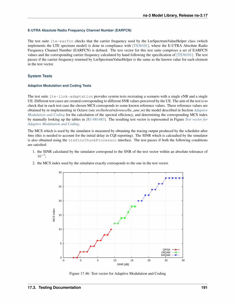
ns-3 Model Library, Release ns-3.17
E-UTRA Absolute Radio Frequency Channel Number (EARFCN)
The test suite lte-earfcn checks that the carrier frequency used by the LteSpectrumValueHelper class (whichimplements the LTE spectrum model) is done in compliance with [TS36101], where the E-UTRA Absolute RadioFrequency Channel Number (EARFCN) is defined. The test vector for this test suite comprises a set of EARFCNvalues and the corresponding carrier frequency calculated by hand following the specification of [TS36101]. The testpasses if the carrier frequency returned by LteSpectrumValueHelper is the same as the known value for each elementin the test vector.
System Tests
Adaptive Modulation and Coding Tests
The test suite lte-link-adaptation provides system tests recreating a scenario with a single eNB and a singleUE. Different test cases are created corresponding to different SNR values perceived by the UE. The aim of the test is tocheck that in each test case the chosen MCS corresponds to some known reference values. These reference values areobtained by re-implementing in Octave (see src/lte/test/reference/lte_amc.m) the model described in Section AdaptiveModulation and Coding for the calculation of the spectral efficiency, and determining the corresponding MCS indexby manually looking up the tables in [R1-081483]. The resulting test vector is represented in Figure Test vector forAdaptive Modulation and Coding.
The MCS which is used by the simulator is measured by obtaining the tracing output produced by the scheduler after4ms (this is needed to account for the initial delay in CQI reporting). The SINR which is calcualted by the simulatoris also obtained using the LteSinrChunkProcessor interface. The test passes if both the following conditionsare satisfied:
1. the SINR calculated by the simulator correspond to the SNR of the test vector within an absolute tolerance of10−7;
2. the MCS index used by the simulator exactly corresponds to the one in the test vector.
0
5
10
15
20
25
30
-5 0 5 10 15 20 25 30
MC
S in
dex
SINR [dB]
QPSK16QAM64QAM
Figure 17.46: Test vector for Adaptive Modulation and Coding
17.3. Testing Documentation 191
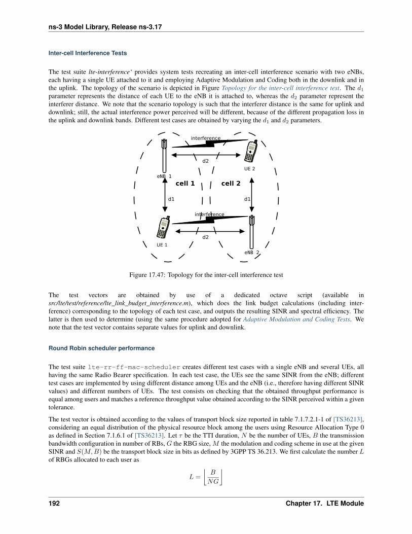
ns-3 Model Library, Release ns-3.17
Inter-cell Interference Tests
The test suite lte-interference‘ provides system tests recreating an inter-cell interference scenario with two eNBs,each having a single UE attached to it and employing Adaptive Modulation and Coding both in the downlink and inthe uplink. The topology of the scenario is depicted in Figure Topology for the inter-cell interference test. The d1
parameter represents the distance of each UE to the eNB it is attached to, whereas the d2 parameter represent theinterferer distance. We note that the scenario topology is such that the interferer distance is the same for uplink anddownlink; still, the actual interference power perceived will be different, because of the different propagation loss inthe uplink and downlink bands. Different test cases are obtained by varying the d1 and d2 parameters.
Figure 17.47: Topology for the inter-cell interference test
The test vectors are obtained by use of a dedicated octave script (available insrc/lte/test/reference/lte_link_budget_interference.m), which does the link budget calculations (including inter-ference) corresponding to the topology of each test case, and outputs the resulting SINR and spectral efficiency. Thelatter is then used to determine (using the same procedure adopted for Adaptive Modulation and Coding Tests. Wenote that the test vector contains separate values for uplink and downlink.
Round Robin scheduler performance
The test suite lte-rr-ff-mac-scheduler creates different test cases with a single eNB and several UEs, allhaving the same Radio Bearer specification. In each test case, the UEs see the same SINR from the eNB; differenttest cases are implemented by using different distance among UEs and the eNB (i.e., therefore having different SINRvalues) and different numbers of UEs. The test consists on checking that the obtained throughput performance isequal among users and matches a reference throughput value obtained according to the SINR perceived within a giventolerance.
The test vector is obtained according to the values of transport block size reported in table 7.1.7.2.1-1 of [TS36213],considering an equal distribution of the physical resource block among the users using Resource Allocation Type 0as defined in Section 7.1.6.1 of [TS36213]. Let τ be the TTI duration, N be the number of UEs, B the transmissionbandwidth configuration in number of RBs, G the RBG size, M the modulation and coding scheme in use at the givenSINR and S(M,B) be the transport block size in bits as defined by 3GPP TS 36.213. We first calculate the number Lof RBGs allocated to each user as
L =⌊B
NG
⌋
192 Chapter 17. LTE Module
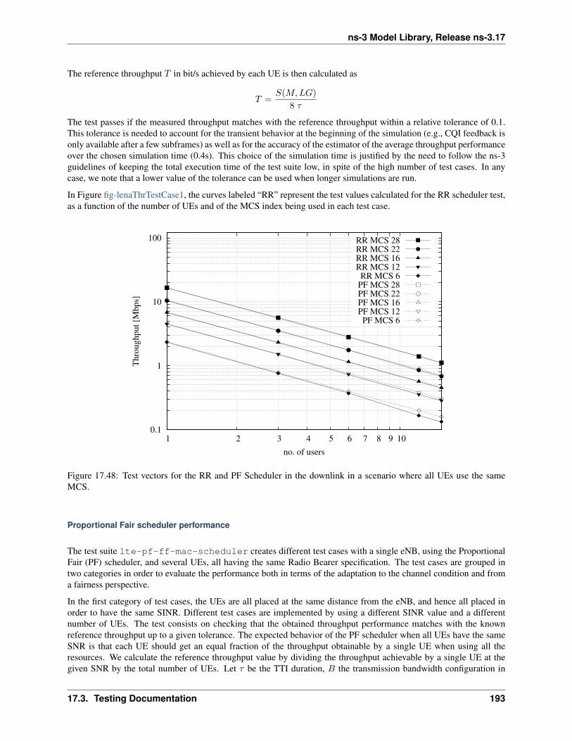
ns-3 Model Library, Release ns-3.17
The reference throughput T in bit/s achieved by each UE is then calculated as
T =S(M,LG)
8 τ
The test passes if the measured throughput matches with the reference throughput within a relative tolerance of 0.1.This tolerance is needed to account for the transient behavior at the beginning of the simulation (e.g., CQI feedback isonly available after a few subframes) as well as for the accuracy of the estimator of the average throughput performanceover the chosen simulation time (0.4s). This choice of the simulation time is justified by the need to follow the ns-3guidelines of keeping the total execution time of the test suite low, in spite of the high number of test cases. In anycase, we note that a lower value of the tolerance can be used when longer simulations are run.
In Figure fig-lenaThrTestCase1, the curves labeled “RR” represent the test values calculated for the RR scheduler test,as a function of the number of UEs and of the MCS index being used in each test case.
0.1
1
10
100
1 2 3 4 5 6 7 8 9 10
Thro
ughput
[Mbps]
no. of users
RR MCS 28RR MCS 22RR MCS 16RR MCS 12RR MCS 6
PF MCS 28PF MCS 22PF MCS 16PF MCS 12PF MCS 6
Figure 17.48: Test vectors for the RR and PF Scheduler in the downlink in a scenario where all UEs use the sameMCS.
Proportional Fair scheduler performance
The test suite lte-pf-ff-mac-scheduler creates different test cases with a single eNB, using the ProportionalFair (PF) scheduler, and several UEs, all having the same Radio Bearer specification. The test cases are grouped intwo categories in order to evaluate the performance both in terms of the adaptation to the channel condition and froma fairness perspective.
In the first category of test cases, the UEs are all placed at the same distance from the eNB, and hence all placed inorder to have the same SINR. Different test cases are implemented by using a different SINR value and a differentnumber of UEs. The test consists on checking that the obtained throughput performance matches with the knownreference throughput up to a given tolerance. The expected behavior of the PF scheduler when all UEs have the sameSNR is that each UE should get an equal fraction of the throughput obtainable by a single UE when using all theresources. We calculate the reference throughput value by dividing the throughput achievable by a single UE at thegiven SNR by the total number of UEs. Let τ be the TTI duration, B the transmission bandwidth configuration in
17.3. Testing Documentation 193
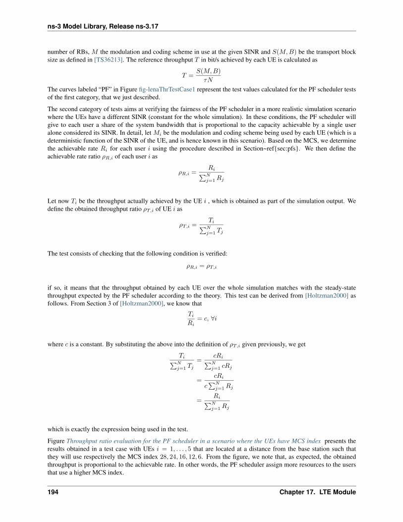
ns-3 Model Library, Release ns-3.17
number of RBs, M the modulation and coding scheme in use at the given SINR and S(M,B) be the transport blocksize as defined in [TS36213]. The reference throughput T in bit/s achieved by each UE is calculated as
T =S(M,B)τN
The curves labeled “PF” in Figure fig-lenaThrTestCase1 represent the test values calculated for the PF scheduler testsof the first category, that we just described.
The second category of tests aims at verifying the fairness of the PF scheduler in a more realistic simulation scenariowhere the UEs have a different SINR (constant for the whole simulation). In these conditions, the PF scheduler willgive to each user a share of the system bandwidth that is proportional to the capacity achievable by a single useralone considered its SINR. In detail, let Mi be the modulation and coding scheme being used by each UE (which is adeterministic function of the SINR of the UE, and is hence known in this scenario). Based on the MCS, we determinethe achievable rate Ri for each user i using the procedure described in Section~ref{sec:pfs}. We then define theachievable rate ratio ρR,i of each user i as
ρR,i =Ri∑Nj=1Rj
Let now Ti be the throughput actually achieved by the UE i , which is obtained as part of the simulation output. Wedefine the obtained throughput ratio ρT,i of UE i as
ρT,i =Ti∑Nj=1 Tj
The test consists of checking that the following condition is verified:
ρR,i = ρT,i
if so, it means that the throughput obtained by each UE over the whole simulation matches with the steady-statethroughput expected by the PF scheduler according to the theory. This test can be derived from [Holtzman2000] asfollows. From Section 3 of [Holtzman2000], we know that
TiRi
= c, ∀i
where c is a constant. By substituting the above into the definition of ρT,i given previously, we get
Ti∑Nj=1 Tj
=cRi∑Nj=1 cRj
=cRi
c∑Nj=1Rj
=Ri∑Nj=1Rj
which is exactly the expression being used in the test.
Figure Throughput ratio evaluation for the PF scheduler in a scenario where the UEs have MCS index presents theresults obtained in a test case with UEs i = 1, . . . , 5 that are located at a distance from the base station such thatthey will use respectively the MCS index 28, 24, 16, 12, 6. From the figure, we note that, as expected, the obtainedthroughput is proportional to the achievable rate. In other words, the PF scheduler assign more resources to the usersthat use a higher MCS index.
194 Chapter 17. LTE Module
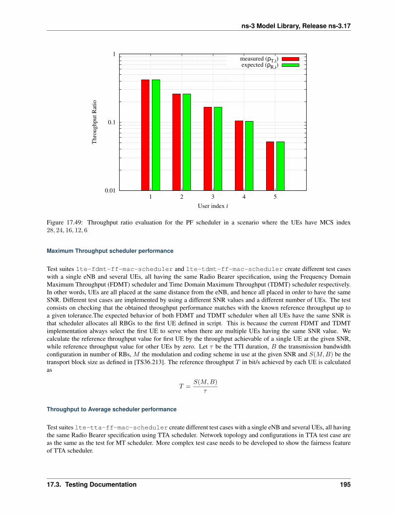
ns-3 Model Library, Release ns-3.17
0.01
0.1
1
1 2 3 4 5
Thro
ughput
Rat
io
User index i
measured (ρT,i)expected (ρR,i)
Figure 17.49: Throughput ratio evaluation for the PF scheduler in a scenario where the UEs have MCS index28, 24, 16, 12, 6
Maximum Throughput scheduler performance
Test suites lte-fdmt-ff-mac-scheduler and lte-tdmt-ff-mac-scheduler create different test caseswith a single eNB and several UEs, all having the same Radio Bearer specification, using the Frequency DomainMaximum Throughput (FDMT) scheduler and Time Domain Maximum Throughput (TDMT) scheduler respectively.In other words, UEs are all placed at the same distance from the eNB, and hence all placed in order to have the sameSNR. Different test cases are implemented by using a different SNR values and a different number of UEs. The testconsists on checking that the obtained throughput performance matches with the known reference throughput up toa given tolerance.The expected behavior of both FDMT and TDMT scheduler when all UEs have the same SNR isthat scheduler allocates all RBGs to the first UE defined in script. This is because the current FDMT and TDMTimplementation always select the first UE to serve when there are multiple UEs having the same SNR value. Wecalculate the reference throughput value for first UE by the throughput achievable of a single UE at the given SNR,while reference throughput value for other UEs by zero. Let τ be the TTI duration, B the transmission bandwidthconfiguration in number of RBs, M the modulation and coding scheme in use at the given SNR and S(M,B) be thetransport block size as defined in [TS36.213]. The reference throughput T in bit/s achieved by each UE is calculatedas
T =S(M,B)
τ
Throughput to Average scheduler performance
Test suites lte-tta-ff-mac-scheduler create different test cases with a single eNB and several UEs, all havingthe same Radio Bearer specification using TTA scheduler. Network topology and configurations in TTA test case areas the same as the test for MT scheduler. More complex test case needs to be developed to show the fairness featureof TTA scheduler.
17.3. Testing Documentation 195
ns-3 Model Library, Release ns-3.17
Blind Average Throughput scheduler performance
Test suites lte-tdbet-ff-mac-scheduler and lte-fdbet-ff-mac-scheduler create different testcases with a single eNB and several UEs, all having the same Radio Bearer specification.
In the first test case of lte-tdbet-ff-mac-scheduler and lte-fdbet-ff-mac-scheduler, the UEs areall placed at the same distance from the eNB, and hence all placed in order to have the same SNR. Different test casesare implemented by using a different SNR value and a different number of UEs. The test consists on checking that theobtained throughput performance matches with the known reference throughput up to a given tolerance. In long term,the expected behavior of both TD-BET and FD-BET when all UEs have the same SNR is that each UE should get anequal throughput. However, the exact throughput value of TD-BET and FD-BET in this test case is not the same.
When all UEs have the same SNR, TD-BET can be seen as a specific case of PF where achievable rate equals to1. Therefore, the throughput obtained by TD-BET is equal to that of PF. On the other hand, FD-BET performs verysimilar to the round robin (RR) scheduler in case of that all UEs have the same SNR and the number of UE( or RBG)is an integer multiple of the number of RBG( or UE). In this case, FD-BET always allocate the same number of RBGsto each UE. For example, if eNB has 12 RBGs and there are 6 UEs, then each UE will get 2 RBGs in each TTI. Orif eNB has 12 RBGs and there are 24 UEs, then each UE will get 2 RBGs per two TTIs. When the number of UE(RBG) is not an integer multiple of the number of RBG (UE), FD-BET will not follow the RR behavior because it willassigned different number of RBGs to some UEs, while the throughput of each UE is still the same.
The second category of tests aims at verifying the fairness of the both TD-BET and FD-BET schedulers in a morerealistic simulation scenario where the UEs have a different SNR (constant for the whole simulation). In this case,both scheduler should give the same amount of averaged throughput to each user.
Specifically, for TD-BET, let Fi be the fraction of time allocated to user i in total simulation time, Rfbi be the the fullbandwidth achievable rate for user i and Ti be the achieved throughput of user i. Then we have:
Ti = FiRfbi
In TD-BET, the sum of Fi for all user equals one. In long term, all UE has the same Ti so that we replace Ti by T .Then we have:
T =1∑N
i=11
Rfbi
Token Band Fair Queue scheduler performance
Test suites lte-fdtbfq-ff-mac-scheduler and lte-tdtbfq-ff-mac-scheduler create different testcases for testing three key features of TBFQ scheduler: traffic policing, fairness and traffic balance. Constant Bit RateUDP traffic is used in both downlink and uplink in all test cases. The packet interval is set to 1ms to keep the RLCbuffer non-empty. Different traffic rate is achieved by setting different packet size. Specifically, two classes of flowsare created in the testsuites:
• Homogeneous flow: flows with the same token generation rate and packet arrival rate
• Heterogeneous flow: flows with different packet arrival rate, but with the same token generation rate
In test case 1 verifies traffic policing and fairness features for the scenario that all UEs are placed at the same distancefrom the eNB. In this case, all Ues have the same SNR value. Different test cases are implemented by using a differentSNR value and a different number of UEs. Because each flow have the same traffic rate and token generation rate,TBFQ scheduler will guarantee the same throughput among UEs without the constraint of token generation rate. Inaddition, the exact value of UE throughput is depended on the total traffic rate:
• If total traffic rate <= maximum throughput, UE throughput = traffic rate
• If total traffic rate > maximum throughput, UE throughput = maximum throughput / N
196 Chapter 17. LTE Module
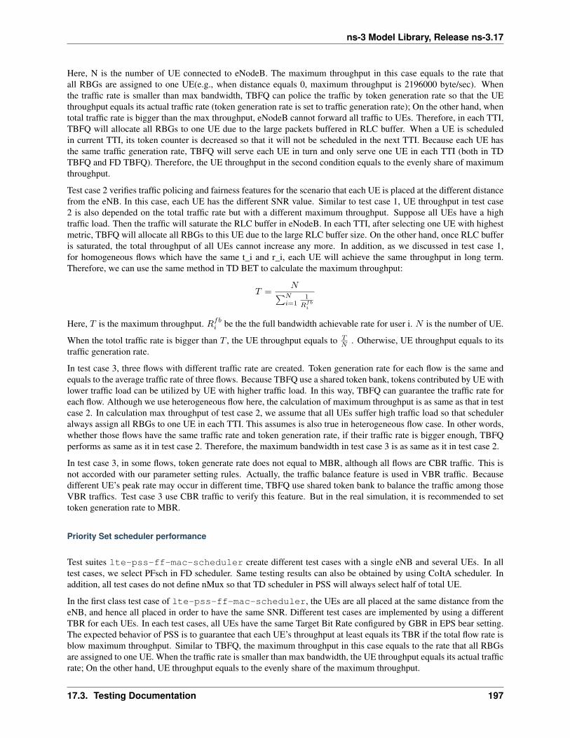
ns-3 Model Library, Release ns-3.17
Here, N is the number of UE connected to eNodeB. The maximum throughput in this case equals to the rate thatall RBGs are assigned to one UE(e.g., when distance equals 0, maximum throughput is 2196000 byte/sec). Whenthe traffic rate is smaller than max bandwidth, TBFQ can police the traffic by token generation rate so that the UEthroughput equals its actual traffic rate (token generation rate is set to traffic generation rate); On the other hand, whentotal traffic rate is bigger than the max throughput, eNodeB cannot forward all traffic to UEs. Therefore, in each TTI,TBFQ will allocate all RBGs to one UE due to the large packets buffered in RLC buffer. When a UE is scheduledin current TTI, its token counter is decreased so that it will not be scheduled in the next TTI. Because each UE hasthe same traffic generation rate, TBFQ will serve each UE in turn and only serve one UE in each TTI (both in TDTBFQ and FD TBFQ). Therefore, the UE throughput in the second condition equals to the evenly share of maximumthroughput.
Test case 2 verifies traffic policing and fairness features for the scenario that each UE is placed at the different distancefrom the eNB. In this case, each UE has the different SNR value. Similar to test case 1, UE throughput in test case2 is also depended on the total traffic rate but with a different maximum throughput. Suppose all UEs have a hightraffic load. Then the traffic will saturate the RLC buffer in eNodeB. In each TTI, after selecting one UE with highestmetric, TBFQ will allocate all RBGs to this UE due to the large RLC buffer size. On the other hand, once RLC bufferis saturated, the total throughput of all UEs cannot increase any more. In addition, as we discussed in test case 1,for homogeneous flows which have the same t_i and r_i, each UE will achieve the same throughput in long term.Therefore, we can use the same method in TD BET to calculate the maximum throughput:
T =N∑N
i=11
Rfbi
Here, T is the maximum throughput. Rfbi be the the full bandwidth achievable rate for user i. N is the number of UE.
When the totol traffic rate is bigger than T , the UE throughput equals to TN . Otherwise, UE throughput equals to its
traffic generation rate.
In test case 3, three flows with different traffic rate are created. Token generation rate for each flow is the same andequals to the average traffic rate of three flows. Because TBFQ use a shared token bank, tokens contributed by UE withlower traffic load can be utilized by UE with higher traffic load. In this way, TBFQ can guarantee the traffic rate foreach flow. Although we use heterogeneous flow here, the calculation of maximum throughput is as same as that in testcase 2. In calculation max throughput of test case 2, we assume that all UEs suffer high traffic load so that scheduleralways assign all RBGs to one UE in each TTI. This assumes is also true in heterogeneous flow case. In other words,whether those flows have the same traffic rate and token generation rate, if their traffic rate is bigger enough, TBFQperforms as same as it in test case 2. Therefore, the maximum bandwidth in test case 3 is as same as it in test case 2.
In test case 3, in some flows, token generate rate does not equal to MBR, although all flows are CBR traffic. This isnot accorded with our parameter setting rules. Actually, the traffic balance feature is used in VBR traffic. Becausedifferent UE’s peak rate may occur in different time, TBFQ use shared token bank to balance the traffic among thoseVBR traffics. Test case 3 use CBR traffic to verify this feature. But in the real simulation, it is recommended to settoken generation rate to MBR.
Priority Set scheduler performance
Test suites lte-pss-ff-mac-scheduler create different test cases with a single eNB and several UEs. In alltest cases, we select PFsch in FD scheduler. Same testing results can also be obtained by using CoItA scheduler. Inaddition, all test cases do not define nMux so that TD scheduler in PSS will always select half of total UE.
In the first class test case of lte-pss-ff-mac-scheduler, the UEs are all placed at the same distance from theeNB, and hence all placed in order to have the same SNR. Different test cases are implemented by using a differentTBR for each UEs. In each test cases, all UEs have the same Target Bit Rate configured by GBR in EPS bear setting.The expected behavior of PSS is to guarantee that each UE’s throughput at least equals its TBR if the total flow rate isblow maximum throughput. Similar to TBFQ, the maximum throughput in this case equals to the rate that all RBGsare assigned to one UE. When the traffic rate is smaller than max bandwidth, the UE throughput equals its actual trafficrate; On the other hand, UE throughput equals to the evenly share of the maximum throughput.
17.3. Testing Documentation 197
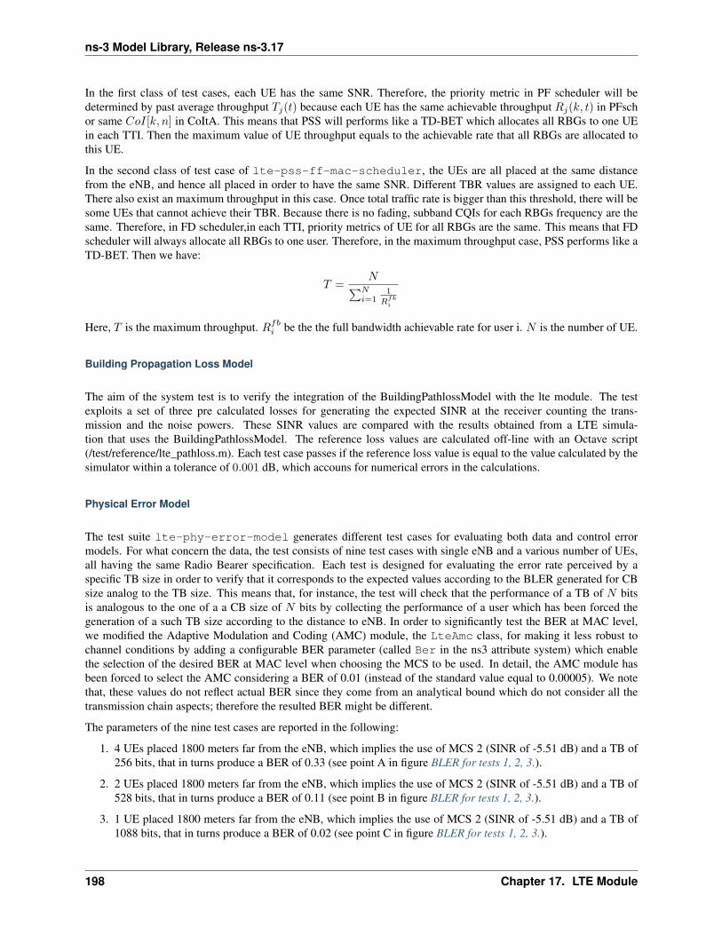
ns-3 Model Library, Release ns-3.17
In the first class of test cases, each UE has the same SNR. Therefore, the priority metric in PF scheduler will bedetermined by past average throughput Tj(t) because each UE has the same achievable throughput Rj(k, t) in PFschor same CoI[k, n] in CoItA. This means that PSS will performs like a TD-BET which allocates all RBGs to one UEin each TTI. Then the maximum value of UE throughput equals to the achievable rate that all RBGs are allocated tothis UE.
In the second class of test case of lte-pss-ff-mac-scheduler, the UEs are all placed at the same distancefrom the eNB, and hence all placed in order to have the same SNR. Different TBR values are assigned to each UE.There also exist an maximum throughput in this case. Once total traffic rate is bigger than this threshold, there will besome UEs that cannot achieve their TBR. Because there is no fading, subband CQIs for each RBGs frequency are thesame. Therefore, in FD scheduler,in each TTI, priority metrics of UE for all RBGs are the same. This means that FDscheduler will always allocate all RBGs to one user. Therefore, in the maximum throughput case, PSS performs like aTD-BET. Then we have:
T =N∑N
i=11
Rfbi
Here, T is the maximum throughput. Rfbi be the the full bandwidth achievable rate for user i. N is the number of UE.
Building Propagation Loss Model
The aim of the system test is to verify the integration of the BuildingPathlossModel with the lte module. The testexploits a set of three pre calculated losses for generating the expected SINR at the receiver counting the trans-mission and the noise powers. These SINR values are compared with the results obtained from a LTE simula-tion that uses the BuildingPathlossModel. The reference loss values are calculated off-line with an Octave script(/test/reference/lte_pathloss.m). Each test case passes if the reference loss value is equal to the value calculated by thesimulator within a tolerance of 0.001 dB, which accouns for numerical errors in the calculations.
Physical Error Model
The test suite lte-phy-error-model generates different test cases for evaluating both data and control errormodels. For what concern the data, the test consists of nine test cases with single eNB and a various number of UEs,all having the same Radio Bearer specification. Each test is designed for evaluating the error rate perceived by aspecific TB size in order to verify that it corresponds to the expected values according to the BLER generated for CBsize analog to the TB size. This means that, for instance, the test will check that the performance of a TB of N bitsis analogous to the one of a a CB size of N bits by collecting the performance of a user which has been forced thegeneration of a such TB size according to the distance to eNB. In order to significantly test the BER at MAC level,we modified the Adaptive Modulation and Coding (AMC) module, the LteAmc class, for making it less robust tochannel conditions by adding a configurable BER parameter (called Ber in the ns3 attribute system) which enablethe selection of the desired BER at MAC level when choosing the MCS to be used. In detail, the AMC module hasbeen forced to select the AMC considering a BER of 0.01 (instead of the standard value equal to 0.00005). We notethat, these values do not reflect actual BER since they come from an analytical bound which do not consider all thetransmission chain aspects; therefore the resulted BER might be different.
The parameters of the nine test cases are reported in the following:
1. 4 UEs placed 1800 meters far from the eNB, which implies the use of MCS 2 (SINR of -5.51 dB) and a TB of256 bits, that in turns produce a BER of 0.33 (see point A in figure BLER for tests 1, 2, 3.).
2. 2 UEs placed 1800 meters far from the eNB, which implies the use of MCS 2 (SINR of -5.51 dB) and a TB of528 bits, that in turns produce a BER of 0.11 (see point B in figure BLER for tests 1, 2, 3.).
3. 1 UE placed 1800 meters far from the eNB, which implies the use of MCS 2 (SINR of -5.51 dB) and a TB of1088 bits, that in turns produce a BER of 0.02 (see point C in figure BLER for tests 1, 2, 3.).
198 Chapter 17. LTE Module
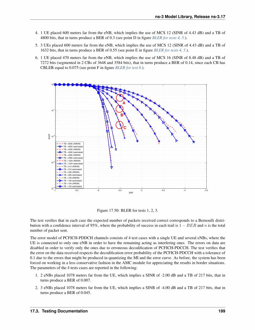
ns-3 Model Library, Release ns-3.17
4. 1 UE placed 600 meters far from the eNB, which implies the use of MCS 12 (SINR of 4.43 dB) and a TB of4800 bits, that in turns produce a BER of 0.3 (see point D in figure BLER for tests 4, 5.).
5. 3 UEs placed 600 meters far from the eNB, which implies the use of MCS 12 (SINR of 4.43 dB) and a TB of1632 bits, that in turns produce a BER of 0.55 (see point E in figure BLER for tests 4, 5.).
6. 1 UE placed 470 meters far from the eNB, which implies the use of MCS 16 (SINR of 8.48 dB) and a TB of7272 bits (segmented in 2 CBs of 3648 and 3584 bits), that in turns produce a BER of 0.14, since each CB hasCBLER equal to 0.075 (see point F in figure BLER for test 6.).
−7 −6.5 −6 −5.5 −5 −4.5 −4 −3.510
−4
10−3
10−2
10−1
100
SNR
BL
ER
TB = 6000 (AWGN)
TB = 6000 (estimated)
TB = 4000 (AWGN)
TB = 4000 (estimated)
TB = 2560 (AWGN)
TB = 2560 (estimated)
TB = 1024 (AWGN)
TB = 1024 (estimated)
TB = 512 (AWGN)
TB = 512 (estimated)
TB = 256 (AWGN)
TB = 256 (estimated)
TB = 160 (AWGN)
TB = 160 (estimated)
TB = 104 (AWGN)
TB = 104 (estimated)
A
B
C
Figure 17.50: BLER for tests 1, 2, 3.
The test verifies that in each case the expected number of packets received correct corresponds to a Bernoulli distri-bution with a confidence interval of 95%, where the probability of success in each trail is 1−BER and n is the totalnumber of packet sent.
The error model of PCFICH-PDDCH channels consists of 4 test cases with a single UE and several eNBs, where theUE is connected to only one eNB in order to have the remaining acting as interfering ones. The errors on data aredisabled in order to verify only the ones due to erroneous decodification of PCFICH-PDCCH. The test verifies thatthe error on the data received respects the decodification error probability of the PCFICH-PDCCH with a tolerance of0.1 due to the errors that might be produced in quantizing the MI and the error curve. As before, the system has beenforced on working in a less conservative fashion in the AMC module for appreciating the results in border situations.The parameters of the 4 tests cases are reported in the following:
1. 2 eNBs placed 1078 meters far from the UE, which implies a SINR of -2.00 dB and a TB of 217 bits, that inturns produce a BER of 0.007.
2. 3 eNBs placed 1078 meters far from the UE, which implies a SINR of -4.00 dB and a TB of 217 bits, that inturns produce a BER of 0.045.
17.3. Testing Documentation 199
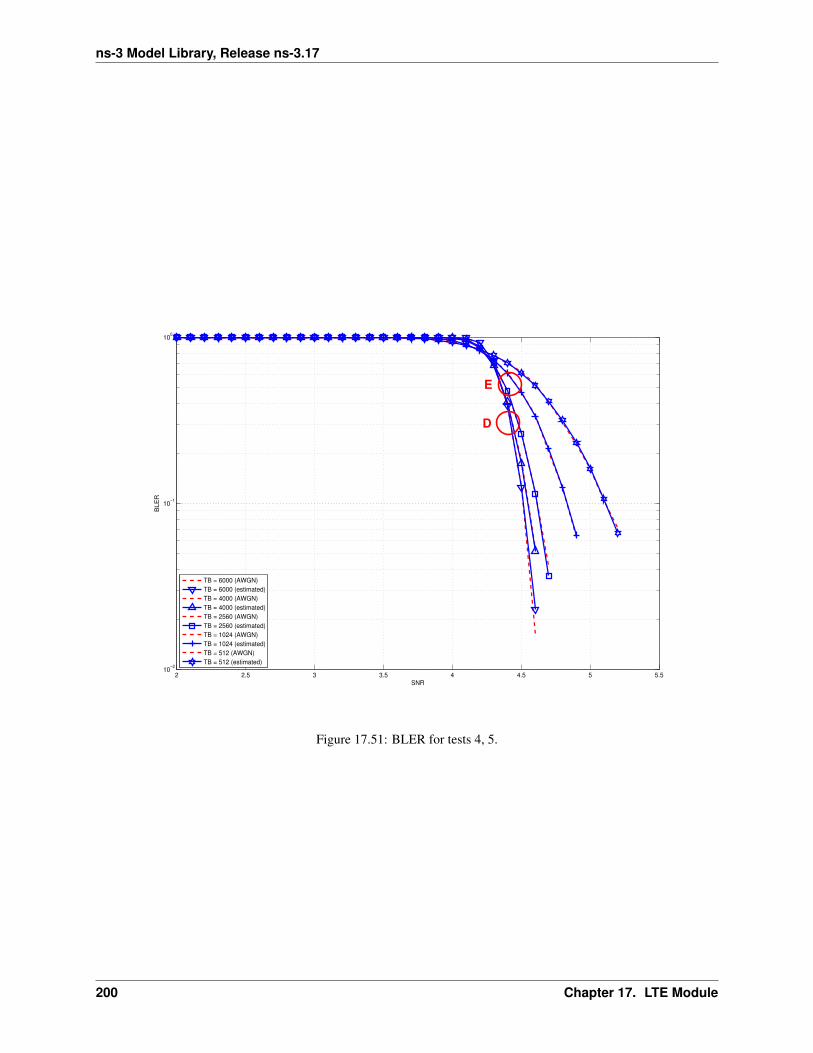
ns-3 Model Library, Release ns-3.17
2 2.5 3 3.5 4 4.5 5 5.510
−2
10−1
100
SNR
BL
ER
TB = 6000 (AWGN)
TB = 6000 (estimated)
TB = 4000 (AWGN)
TB = 4000 (estimated)
TB = 2560 (AWGN)
TB = 2560 (estimated)
TB = 1024 (AWGN)
TB = 1024 (estimated)
TB = 512 (AWGN)
TB = 512 (estimated)
E
D
Figure 17.51: BLER for tests 4, 5.
200 Chapter 17. LTE Module
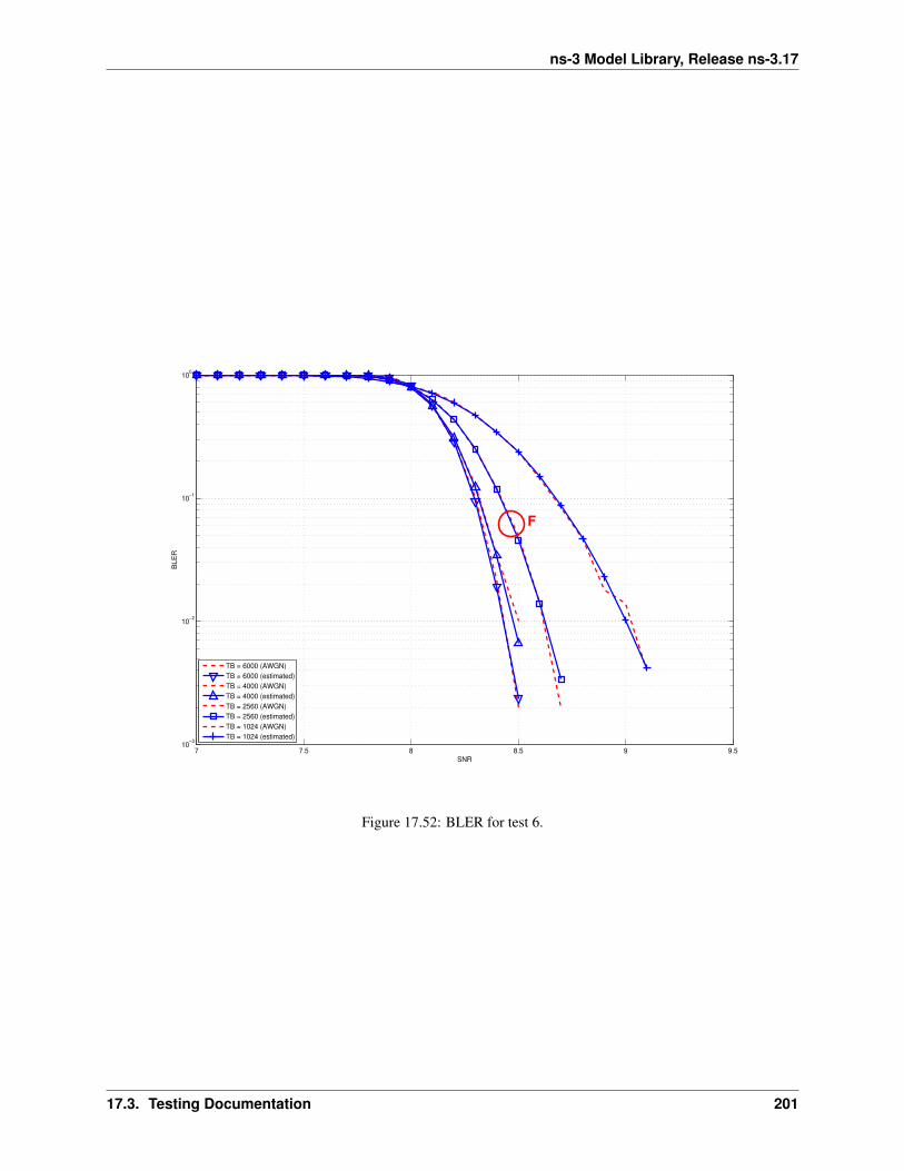
ns-3 Model Library, Release ns-3.17
7 7.5 8 8.5 9 9.510
−3
10−2
10−1
100
SNR
BL
ER
TB = 6000 (AWGN)
TB = 6000 (estimated)
TB = 4000 (AWGN)
TB = 4000 (estimated)
TB = 2560 (AWGN)
TB = 2560 (estimated)
TB = 1024 (AWGN)
TB = 1024 (estimated)
F
Figure 17.52: BLER for test 6.
17.3. Testing Documentation 201
ns-3 Model Library, Release ns-3.17
3. 4 eNBs placed 1078 meters far from the UE, which implies a SINR of -6.00 dB and a TB of 133 bits, that inturns produce a BER of 0.206.
4. 5 eNBs placed 1078 meters far from the UE, which implies a SINR of -7.00 dB and a TB of 81 bits, that in turnsproduce a BER of 0.343.
HARQ Model
The test suite lte-harq includes two tests for evaluating the HARQ model and the related extension in the errormodel. The test consists on checking whether the amount of bytes received during the simulation corresponds to theexpected ones according to the values of transport block and the HARQ dynamics. In detail, the test checks whetherthe throughput obtained after one HARQ retransmission is the expeted one. For evaluating the expected throughputthe expected TB delivering time has been evaluated according to the following formula:
T = P 1s × 1 + P 2
s × 2 + (1− P 2s )× 3
where P is is the probability of receiving with success the HARQ block at the attempt i (i.e., the RV with 3GPP naming).According to the scenarios, in the test we always have P 1
s equal to 0.0, while P 2s varies in the two tests, in detail:
Ttest−1 = 0.0× 1 + 0.77× 2 + 0.23× 3 = 2.23
Ttest−2 = 0.0× 1 + 0.9862× 2 + 0.0138× 3 = 2.0138
The expected throughput is calculted by counting the number of transmission slots available during the simulation(e.g., the number of TTIs) and the size of the TB in the simulation, in detail:
Thrtest−i =TTINUMTtest−i
TBsize =
10002.23
41 = 18375 bps for test-1
10002.0138
469 = 236096 bps for test-2
where TTINUM is the total number of TTIs in 1 second. The test is performed both for Round Robin scheduler. Thetest passes if the measured throughput matches with the reference throughput within a relative tolerance of 0.1. Thistolerance is needed to account for the transient behavior at the beginning of the simulation and the on-fly blocks at theend of the simulation.
MIMO Model
The test suite lte-mimo aims at verifying both the effect of the gain considered for each Transmission Mode onthe system performance and the Transmission Mode switching through the scheduler interface. The test consists onchecking whether the amount of bytes received during a certain window of time (0.1 seconds in our case) correspondsto the expected ones according to the values of transport block size reported in table 7.1.7.2.1-1 of [TS36213], similarlyto what done for the tests of the schedulers.
The test is performed both for Round Robin and Proportional Fair schedulers. The test passes if the measured through-put matches with the reference throughput within a relative tolerance of 0.1. This tolerance is needed to account forthe transient behavior at the beginning of the simulation and the transition phase between the Transmission Modes.
Antenna Model integration
The test suite lte-antenna checks that the AntennaModel integrated with the LTE model works correctly. This testsuite recreates a simulation scenario with one eNB node at coordinates (0,0,0) and one UE node at coordinates (x,y,0).The eNB node is configured with an CosineAntennaModel having given orientation and beamwidth. The UE insteaduses the default IsotropicAntennaModel. The test checks that the received power both in uplink and downlink account
202 Chapter 17. LTE Module
ns-3 Model Library, Release ns-3.17
for the correct value of the antenna gain, which is determined offline; this is implemented by comparing the uplink anddownlink SINR and checking that both match with the reference value up to a tolerance of 10−6 which accounts fornumerical errors. Different test cases are provided by varying the x and y coordinates of the UE, and the beamwidthand the orientation of the antenna of the eNB.
RLC
Two test suites lte-rlc-um-transmitter and lte-rlc-am-transmitter check that the UM RLC andthe AM RLC implementation work correctly. Both these suites work by testing RLC instances connected to specialtest entities that play the role of the MAC and of the PDCP, implementing respectively the LteMacSapProvider andLteRlcSapUser interfaces. Different test cases (i.e., input test vector consisting of series of primitive calls by the MACand the PDCP) are provided that check the behavior in the following cases:
1. one SDU, one PDU: the MAC notifies a TX opportunity causes the creation of a PDU which exactly contains awhole SDU
2. segmentation: the MAC notifies multiple TX opportunities that are smaller than the SDU size stored in thetransmission buffer, which is then to be fragmented and hence multiple PDUs are generated;
3. concatenation: the MAC notifies a TX opportunity that is bigger than the SDU, hence multiple SDUs areconcatenated in the same PDU
4. buffer status report: a series of new SDUs notifications by the PDCP is inteleaved with a series of TX opportunitynotification in order to verify that the buffer status report procedure is correct.
In all these cases, an output test vector is determine manually from knowledge of the input test vector and knowledgeof the expected behavior. These test vector are specialized for UM RLC and AM RLC due to their different behavior.Each test case passes if the sequence of primitives triggered by the RLC instance being tested is exacly equal to theoutput test vector. In particular, for each PDU transmitted by the RLC instance, both the size and the content of thePDU are verified to check for an exact match with the test vector.
RRC
The test suite lte-rrc tests the correct functionality of the following aspects:
1. MAC Random Access
2. RRC System Information Acquisition
3. RRC Connection Establishment
4. RRC Reconfiguration
The test suite considers a type of scenario with a single eNB and multiple UEs that are instructed to connect to theeNB. Each test case implement an instance of this scenario with specific values of the following parameters:
• number of UEs
• number of Data Radio Bearers to be activated for each UE
• time tc0 at which the first UE is instructed to start connecting to the eNB
• time interval di between the start of connection of UE n and UE n+ 1; the time at which user n connects is thusdetermined as tcn = tc0 + ndi sdf
• a boolean flag indicating whether the ideal or the real RRC protocol model is used
17.3. Testing Documentation 203

ns-3 Model Library, Release ns-3.17
Each test cases passes if a number of test conditions are positively evaluated for each UE after a delay de from thetime it started connecting to the eNB. The delay de is determined as
de = dsi + dra + dce + dcr
where:
• dsi is the max delay necessary for the acquisition of System Information. We set it to 90ms accounting for 10msfor the MIB acquisition and 80ms for the subsequent SIB2 acquisition
• dra is the delay for the MAC Random Access (RA) procedure. This depends on preamble collisions as well as onthe availability of resources for the UL grant allocation. The total amount of necessary RA attempts depends onpreamble collisions and failures to allocate the UL grant because of lack of resources. The number of collisionsdepends on the number of UEs that try to access simultaneously; we estimated that for a 0.99 RA success proba-bility, 5 attempts are sufficient for up to 20 UEs, and 10 attempts for up to 50 UEs. For the UL grant, consideredthe system bandwidth and the default MCS used for the UL grant (MCS 0), at most 4 UL grants can be assignedin a TTI; so for n UEs trying to do RA simultaneously the max number of attempts due to the UL grant issue isdn/4e. The time for a RA attempt is determined by 3ms + the value of LteEnbMac::RaResponseWindowSize,which defaults to 3ms, plus 1ms for the scheduling of the new transmission.
• dce is the delay required for the transmission of RRC CONNECTION SETUP + RRC CONNECTION SETUPCOMPLETED. We consider a round trip delay of 10ms plus d2n/4e considering that 2 RRC packets have to betransmitted and that at most 4 such packets can be transmitted per TTI.
• dcr is the delay required for eventually needed RRC CONNECTION RECONFIGURATION transactions. Thenumber of transactions needed is 1 for each bearer activation plus a variable number for SRS reconfigurationthat depends on:math:n:
– 0 for n ≤ 2
– 1 for n ≤ 5
– 2 for n ≤ 10
– 3 for n ≤ 20
– 4 for n > 20
Similarly to what done for dce, for each transaction we consider a round trip delay of 10ms plus d2n/4e. delayof 20ms.
The conditions that are evaluated for a test case to pass are, for each UE:
• the eNB has the context of the UE (identified by the RNTI value retrieved from the UE RRC)
• the RRC state of the UE at the eNB is CONNECTED_NORMALLY
• the RRC state at the UE is CONNECTED_NORMALLY
• the UE is configured with the CellId, DlBandwidth, UlBandwidth, DlEarfcn and UlEarfcn of the eNB
• the IMSI of the UE stored at the eNB is correct
• the number of active Data Radio Bearers is the expected one, both at the eNB and at the UE
• for each Data Radio Bearer, the following identifiers match between the UE and the eNB: EPS bearer id, DRBid, LCID
GTP-U protocol
The unit test suite epc-gtpu checks that the encoding and decoding of the GTP-U header is done correctly. The testfills in a header with a set of known values, adds the header to a packet, and then removes the header from the packet.
204 Chapter 17. LTE Module
ns-3 Model Library, Release ns-3.17
The test fails if, upon removing, any of the fields in the GTP-U header is not decoded correctly. This is detected bycomparing the decoded value from the known value.
S1-U interface
Two test suites (epc-s1u-uplink and epc-s1u-downlink) make sure that the S1-U interface implementationworks correctly in isolation. This is achieved by creating a set of simulation scenarios where the EPC model aloneis used, without the LTE model (i.e., without the LTE radio protocol stack, which is replaced by simple CSMAdevices). This checks that the interoperation between multiple EpcEnbApplication instances in multiple eNBs andthe EpcSgwPgwApplication instance in the SGW/PGW node works correctly in a variety of scenarios, with varyingnumbers of end users (nodes with a CSMA device installed), eNBs, and different traffic patterns (packet sizes andnumber of total packets). Each test case works by injecting the chosen traffic pattern in the network (at the consideredUE or at the remote host for in the uplink or the downlink test suite respectively) and checking that at the receiver (theremote host or each considered UE, respectively) that exactly the same traffic patterns is received. If any mismatch inthe transmitted and received traffic pattern is detected for any UE, the test fails.
TFT classifier
The test suite epc-tft-classifier checks in isolation that the behavior of the EpcTftClassifier class is correct.This is performed by creating different classifier instances where different TFT instances are activated, and testing foreach classifier that an heterogeneous set of packets (including IP and TCP/UDP headers) is classified correctly. Severaltest cases are provided that check the different matching aspects of a TFT (e.g. local/remote IP address, local/remoteport) both for uplink and downlink traffic. Each test case corresponds to a specific packet and a specific classifierinstance with a given set of TFTs. The test case passes if the bearer identifier returned by the classifier exactly matcheswith the one that is expected for the considered packet.
End-to-end LTE-EPC data plane functionality
The test suite lte-epc-e2e-data ensures the correct end-to-end functionality of the LTE-EPC data plane. Foreach test case in this suite, a complete LTE-EPC simulation scenario is created with the following characteristics:
• a given number of eNBs
• for each eNB, a given number of UEs
• for each UE, a given number of active EPS bearers
• for each active EPS bearer, a given traffic pattern (number of UDP packets to be transmitted and packet size)
Each test is executed by transmitting the given traffic pattern both in the uplink and in the downlink, at subsequenttime intervals. The test passes if all the following conditions are satisfied:
• for each active EPS bearer, the transmitted and received traffic pattern (respectively at the UE and the remotehost for uplink, and vice versa for downlink) is exactly the same
• for each active EPS bearer and each direction (uplink or downlink), exactly the expected number of packet flowsover the corresponding RadioBearer instance
X2 handover
The test suite lte-x2-handover checks the correct functionality of the X2 handover procedure. The scenariobeing tested is a topology with two eNBs connected by an X2 interface. Each test case is a particular instance of thisscenario defined by the following parameters:
17.3. Testing Documentation 205

ns-3 Model Library, Release ns-3.17
• the number of UEs that are initially attached to the first eNB
• the number of EPS bearers activated for each UE
• a list of handover events to be triggered, where each event is defined by: + the start time of the handover trigger+ the index of the UE doing the handover + the index of the source eNB + the index of the target eNB
• a boolean flag indicating whether the target eNB admits the handover or not
• a boolean flag indicating whether the ideal RRC protocol is to be used instead of the real RRC protocol
• the type of scheduler to be used (RR or PF)
Each test cases passes if the following conditions are true:
• at time 0.06s, the test CheckConnected verifies that each UE is connected to the first eNB
• for each event in the handover list:
– at the indicated event start time, the indicated UE is connected to the indicated source eNB
– 0.1s after the start time, the indicated UE is connected to the indicated target eNB
– 0.6s after the start time, for each active EPS bearer, the uplink and downlink sink applications of theindicated UE have achieved a number of bytes which is at least half the number of bytes transmitted bythe corresponding source applications
The condition “UE is connected to eNB” is evaluated positively if and only if all the following conditions are met:
• the eNB has the context of the UE (identified by the RNTI value retrieved from the UE RRC)
• the RRC state of the UE at the eNB is CONNECTED_NORMALLY
• the RRC state at the UE is CONNECTED_NORMALLY
• the UE is configured with the CellId, DlBandwidth, UlBandwidth, DlEarfcn and UlEarfcn of the eNB
• the IMSI of the UE stored at the eNB is correct
• the number of active Data Radio Bearers is the expected one, both at the eNB and at the UE
• for each Data Radio Bearer, the following identifiers match between the UE and the eNB: EPS bearer id, DRBid, LCID
Handover delays
Handover procedure consists of several message exchanges between UE, source eNodeB, and target eNodeB over bothRRC protocol and X2 interface. Test suite lte-handover-delay verifies that this procedure consistently spendsthe same amount of time.
The test suite will run several handover test cases. Eact test case is an individual simulation featuring a handover at aspecified time in simulation. For example, the handover in the first test case is invoked at time +0.100s, while in thesecond test case it is at +0.101s. There are 10 test cases, each testing a different subframe in LTE. Thus the last testcase has the handover at +0.109s.
The simulation scenario in the test cases is as follow:
• EPC is enabled
• 2 eNodeBs with circular (isotropic) antenna, separated by 1000 meters
• 1 static UE positioned exactly in the center between the eNodeBs
• no application installed
• no channel fading
206 Chapter 17. LTE Module
ns-3 Model Library, Release ns-3.17
• default path loss model (Friis)
• 0.300s simulation duration
The test case runs as follow. At the beginning of the simulation, the UE is attached to the first eNodeB. Then at thetime specified by the test case input argument, a handover request will be explicitly issued to the second eNodeB. Thetest case will then record the starting time, wait until the handover is completed, and then record the completion time.If the difference between the completion time and starting time is less than a predefined threshold, then the test passes.
A typical handover in the current ns-3 implementation takes 4.2141 ms when using Ideal RRC protocol model, and19.9283 ms when using Real RRC protocol model. Accordingly, the test cases use 5 ms and 20 ms as the maximumthreshold values. The test suite runs 10 test cases with Ideal RRC protocol model and 10 test cases with Real RRCprotocol model. More information regarding these models can be found in Section RRC protocol models.
The motivation behind using subframes as the main test parameters is the fact that subframe index is one of the factorsfor calculating RA-RNTI, which is used by Random Access during the handover procedure. The test cases verifythis computation, utilizing the fact that the handover will be delayed when this computation is broken. In the defaultsimulation configuration, the handover delay observed because of a broken RA-RNTI computation is typically 6 ms.
17.4 Profiling Documentation
17.4.1 Overview and objectives
The main objective of the profiling carried out is to assess the simulator performance on a broad set of scenarios. Thisevaluation provides reference values for simulation running times and memory consumption figures. It also helps toidentify potential performance improvements and to check for scalability problems when increasing the number ofeNodeB and UEs attached to those.
In the following sections, a detailed description of the general profiling framework employed to perform the study isintroduced. It also includes details on the main performed tests and its results evaluation.
17.4.2 Framework description
Simulation scripts
The simulation script used for all the E-UTRAN results showed in this documentation is located atsrc/lte/examples/lena-profiling.cc. It uses the complete PHY and MAC UE/eNodeB implementa-tion with a simplified RLC implementation on top. This script generates a squared grid topology, placing a eNodeBat the centre of each square. UEs attached to this node are scattered randomly across the square (using a randomuniform distribution along X and Y axis). If BuildingPropagationModel is used, the squares are replaced by rooms.To generate the UL and DL traffic, the RLC implementation always report data to be transfered.
For the EPC results, the script is src/lte/examples/lena-simple-epc.cc. It uses a complete E-UTRANimplementation (PHY+MAC+RLC/UM+PDCP) and the most relevant EPC user plane entities the PGW and SGW,including GTP-U tunneling. This script generates a given number of eNodeBs, distributed across a line and attaches asingle UE to every eNodeB. It also creates an EPC network and an external host connected to it through the Internet.Each UE sends and receives data to and from the remote host. In addition, each UE is also sending data to the UEcamped in the adjacent eNodeB.
RLC and MAC traces are enabled for all UEs and all eNodeBs and those traces are written to disk directly. The MACscheduler used is round robin.
17.4. Profiling Documentation 207
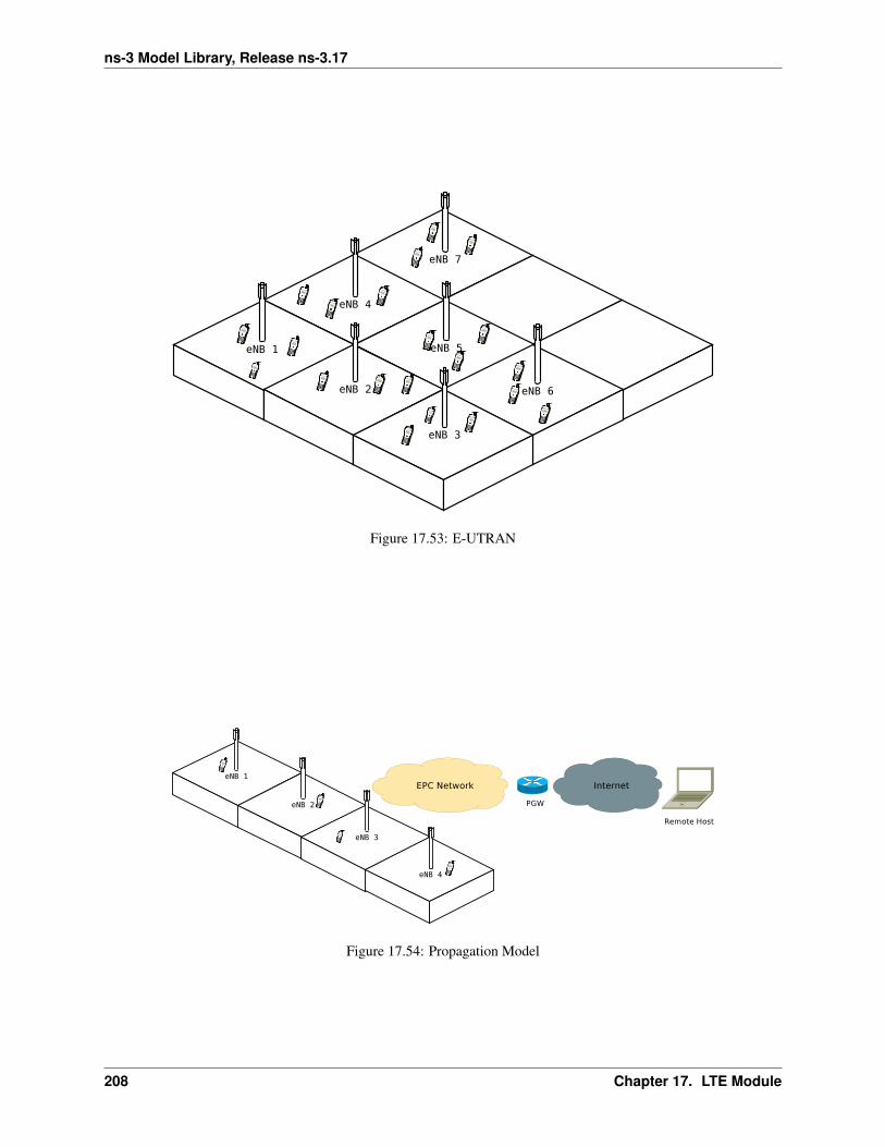
ns-3 Model Library, Release ns-3.17
Figure 17.53: E-UTRAN
Figure 17.54: Propagation Model
208 Chapter 17. LTE Module
ns-3 Model Library, Release ns-3.17
Simulation input parameters
The lena-profiling simulation script accepts the following input parameters:
• simTime: time to simulate (in seconds)
• nUe: number of UEs attached to each eNodeB
• nEnb: number of eNodeB composing the grid per floor
• nFloors: number of floors, 0 for Friis propagation model (no walls), 1 or greater for Building propagationmodel generating a nFloors-storey building.
• traceDirectory: destination directory where simulation traces will be stored
The lena-simple-epc script accepts those other parameters:
• simTime: time to simulate (in seconds)
• numberOfNodes: number of eNodeB + UE pairs created
Time measurement
Running time is measured using default Linux shell command time. This command counts how much user time theexecution of a program takes.
Perl script
To simplify the process of running the profiling script for a wide range of values and collecting itstiming data, a simple Perl script to automate the complete process is provided. It is placed insrc/lte/test/lte-test-run-time.pl for lena-profiling and in src/lte/epc-test-run-time.plfor lena-simple-epc. It simply runs a batch of simulations with a range of parameters and stores the timing resultsin a CSV file called lteTimes.csv and epcTimes.csv respectively. The range of values each parameter sweeps can bemodified editing the corresponding script.
Requirements
The following Perl modules are required to use the provided script, all of them available from CPAN:
• IO::CaptureOutput
• Statistics::Descriptive
For installing the modules, simply use the follwing command:
perl -MCPAN -e ’install moduleName’
Plotting results
To plot the results obtained from running the Perl scripts, two gnuplot scripts are provided, insrc/lte/test/lte-test-run-plot and src/lte/test/epc-test-run-plot. Most of theplots available in this documentation can be reproduced with those, typing the commands gnuplot <src/lte/test/lte-test-run-plot and gnuplot < src/lte/test/epc-test-run-plot.
17.4. Profiling Documentation 209
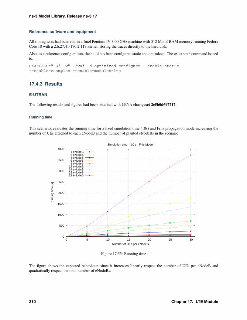
ns-3 Model Library, Release ns-3.17
Reference software and equipment
All timing tests had been run in a Intel Pentium IV 3.00 GHz machine with 512 Mb of RAM memory running FedoraCore 10 with a 2.6.27.41-170.2.117 kernel, storing the traces directly to the hard disk.
Also, as a reference configuration, the build has been configured static and optimized. The exact waf command issuedis:
CXXFLAGS="-O3 -w" ./waf -d optimized configure --enable-static--enable-examples --enable-modules=lte
17.4.3 Results
E-UTRAN
The following results and figures had been obtained with LENA changeset 2c5b0d697717.
Running time
This scenario, evaluates the running time for a fixed simulation time (10s) and Friis propagation mode increasing thenumber of UEs attached to each eNodeB and the number of planted eNodeBs in the scenario.
0
500
1000
1500
2000
2500
3000
3500
4000
0 5 10 15 20 25 30
Run
ning
tim
e [s
]
Number of UEs per eNodeB
Simulation time = 10 s - Friis Model
1 eNodeB2 eNodeB4 eNodeB6 eNodeB8 eNodeB
12 eNodeB14 eNodeB18 eNodeB22 eNodeB
Figure 17.55: Running time
The figure shows the expected behaviour, since it increases linearly respect the number of UEs per eNodeB andquadratically respect the total number of eNodeBs.
210 Chapter 17. LTE Module
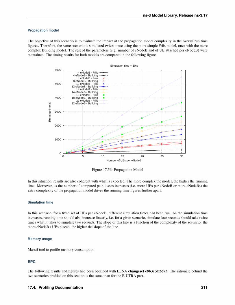
ns-3 Model Library, Release ns-3.17
Propagation model
The objective of this scenario is to evaluate the impact of the propagation model complexity in the overall run timefigures. Therefore, the same scenario is simulated twice: once using the more simple Friis model, once with the morecomplex Building model. The rest of the parameters (e.g. number of eNodeB and of UE attached per eNodeB) weremantained. The timing results for both models are compared in the following figure.
0
1000
2000
3000
4000
5000
6000
0 5 10 15 20 25 30
Run
ning
tim
e [s
]
Number of UEs per eNodeB
Simulation time = 10 s
4 eNodeB - Friis4 eNodeB - Building
8 eNodeB - Friis8 eNodeB - Building
12 eNodeB - Friis12 eNodeB - Building
14 eNodeB - Friis14 eNodeB - Building
18 eNodeB - Friis18 eNodeB - Building
22 eNodeB - Friis22 eNodeB - Building
Figure 17.56: Propagation Model
In this situation, results are also coherent with what is expected. The more complex the model, the higher the runningtime. Moreover, as the number of computed path losses increases (i.e. more UEs per eNodeB or more eNodeBs) theextra complexity of the propagation model drives the running time figures further apart.
Simulation time
In this scenario, for a fixed set of UEs per eNodeB, different simulation times had been run. As the simulation timeincreases, running time should also increase linearly, i.e. for a given scenario, simulate four seconds should take twicetimes what it takes to simulate two seconds. The slope of this line is a function of the complexity of the scenario: themore eNodeB / UEs placed, the higher the slope of the line.
Memory usage
Massif tool to profile memory consumption
EPC
The following results and figures had been obtained with LENA changeset e8b3ccdf6673. The rationale behind thetwo scenarios profiled on this section is the same than for the E-UTRA part.
17.4. Profiling Documentation 211
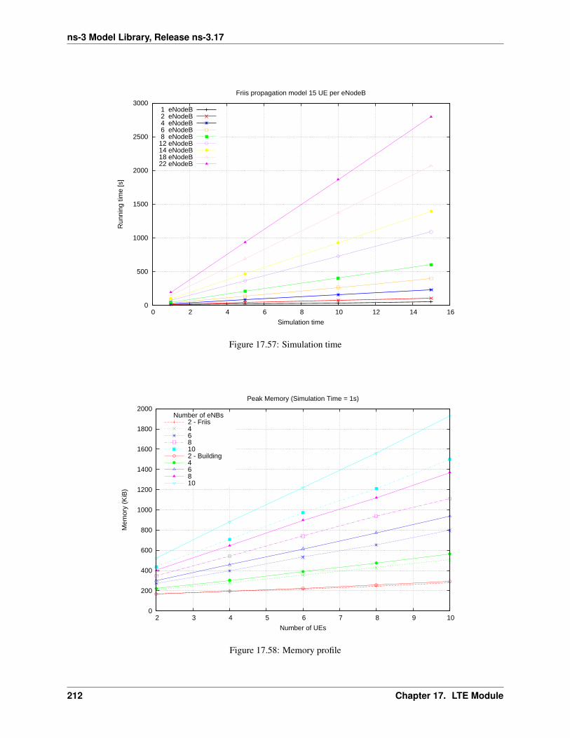
ns-3 Model Library, Release ns-3.17
0
500
1000
1500
2000
2500
3000
0 2 4 6 8 10 12 14 16
Run
ning
tim
e [s
]
Simulation time
Friis propagation model 15 UE per eNodeB
1 eNodeB2 eNodeB4 eNodeB6 eNodeB8 eNodeB
12 eNodeB14 eNodeB18 eNodeB22 eNodeB
Figure 17.57: Simulation time
0
200
400
600
800
1000
1200
1400
1600
1800
2000
2 3 4 5 6 7 8 9 10
Mem
ory
(KiB
)
Number of UEs
Peak Memory (Simulation Time = 1s)
Number of eNBs2 - Friis468102 - Building46810
Figure 17.58: Memory profile
212 Chapter 17. LTE Module
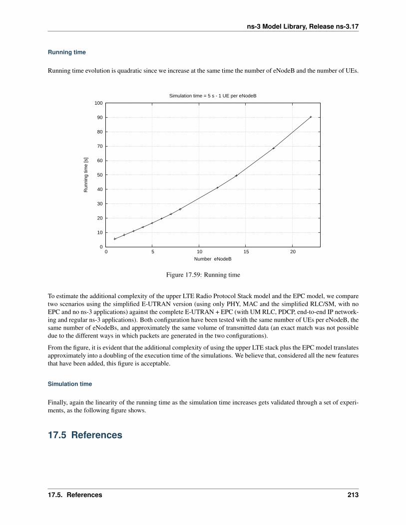
ns-3 Model Library, Release ns-3.17
Running time
Running time evolution is quadratic since we increase at the same time the number of eNodeB and the number of UEs.
0
10
20
30
40
50
60
70
80
90
100
0 5 10 15 20
Run
ning
tim
e [s
]
Number eNodeB
Simulation time = 5 s - 1 UE per eNodeB
Figure 17.59: Running time
To estimate the additional complexity of the upper LTE Radio Protocol Stack model and the EPC model, we comparetwo scenarios using the simplified E-UTRAN version (using only PHY, MAC and the simplified RLC/SM, with noEPC and no ns-3 applications) against the complete E-UTRAN + EPC (with UM RLC, PDCP, end-to-end IP network-ing and regular ns-3 applications). Both configuration have been tested with the same number of UEs per eNodeB, thesame number of eNodeBs, and approximately the same volume of transmitted data (an exact match was not possibledue to the different ways in which packets are generated in the two configurations).
From the figure, it is evident that the additional complexity of using the upper LTE stack plus the EPC model translatesapproximately into a doubling of the execution time of the simulations. We believe that, considered all the new featuresthat have been added, this figure is acceptable.
Simulation time
Finally, again the linearity of the running time as the simulation time increases gets validated through a set of experi-ments, as the following figure shows.
17.5 References
17.5. References 213
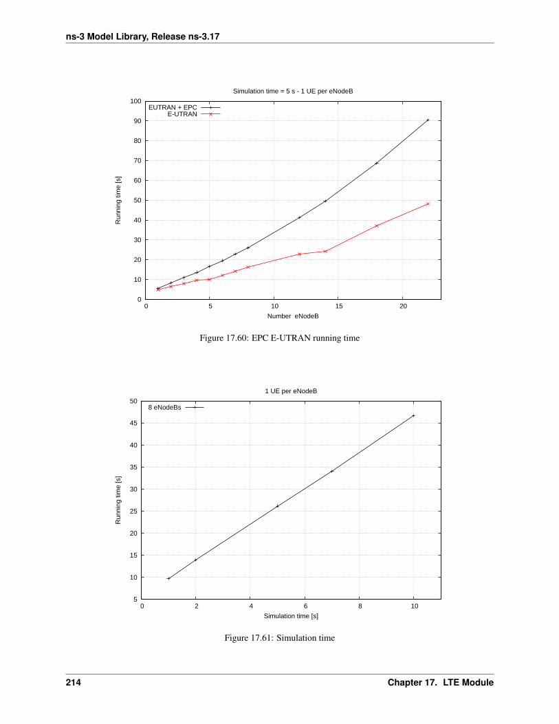
ns-3 Model Library, Release ns-3.17
0
10
20
30
40
50
60
70
80
90
100
0 5 10 15 20
Run
ning
tim
e [s
]
Number eNodeB
Simulation time = 5 s - 1 UE per eNodeB
EUTRAN + EPCE-UTRAN
Figure 17.60: EPC E-UTRAN running time
5
10
15
20
25
30
35
40
45
50
0 2 4 6 8 10
Run
ning
tim
e [s
]
Simulation time [s]
1 UE per eNodeB
8 eNodeBs
Figure 17.61: Simulation time
214 Chapter 17. LTE Module
CHAPTER
EIGHTEEN
MESH NETDEVICE
Placeholder chapter
The Mesh NetDevice based on 802.11s was added in ns-3.6. An overview presentation by Kirill Andreev was pub-lished at the wns-3 workshop in 2009: http://www.nsnam.org/wiki/index.php/Wns3-2009.
215

ns-3 Model Library, Release ns-3.17
216 Chapter 18. Mesh NetDevice
CHAPTER
NINETEEN
MPI FOR DISTRIBUTED SIMULATION
Parallel and distributed discrete event simulation allows the execution of a single simulation program on multipleprocessors. By splitting up the simulation into logical processes, LPs, each LP can be executed by a different proces-sor. This simulation methodology enables very large-scale simulations by leveraging increased processing power andmemory availability. In order to ensure proper execution of a distributed simulation, message passing between LPsis required. To support distributed simulation in ns-3, the standard Message Passing Interface (MPI) is used, alongwith a new distributed simulator class. Currently, dividing a simulation for distributed purposes in ns-3 can only occuracross point-to-point links.
19.1 Current Implementation Details
During the course of a distributed simulation, many packets must cross simulator boundaries. In other words, a packetthat originated on one LP is destined for a different LP, and in order to make this transition, a message containing thepacket contents must be sent to the remote LP. Upon receiving this message, the remote LP can rebuild the packetand proceed as normal. The process of sending an receiving messages between LPs is handled easily by the new MPIinterface in ns-3.
Along with simple message passing between LPs, a distributed simulator is used on each LP to determine whichevents to process. It is important to process events in time-stamped order to ensure proper simulation execution. If aLP receives a message containing an event from the past, clearly this is an issue, since this event could change otherevents which have already been executed. To address this problem, a conservative synchronization algorithm withlookahead is used in ns-3. For more information on different synchronization approaches and parallel and distributedsimulation in general, please refer to “Parallel and Distributed Simulation Systems” by Richard Fujimoto.
19.1.1 Remote point-to-point links
As described in the introduction, dividing a simulation for distributed purposes in ns-3 currently can only occur acrosspoint-to-point links; therefore, the idea of remote point-to-point links is very important for distributed simulation inns-3. When a point-to-point link is installed, connecting two nodes, the point-to-point helper checks the system id, orrank, of both nodes. The rank should be assigned during node creation for distributed simulation and is intended tosignify on which LP a node belongs. If the two nodes are on the same rank, a regular point-to-point link is created. If,however, the two nodes are on different ranks, then these nodes are intended for different LPs, and a remote point-to-point link is used. If a packet is to be sent across a remote point-to-point link, MPI is used to send the message to theremote LP.
217
ns-3 Model Library, Release ns-3.17
19.1.2 Distributing the topology
Currently, the full topology is created on each rank, regardless of the individual node system ids. Only the applica-tions are specific to a rank. For example, consider node 1 on LP 1 and node 2 on LP 2, with a traffic generator onnode 1. Both node 1 and node 2 will be created on both LP1 and LP2; however, the traffic generator will only beinstalled on LP1. While this is not optimal for memory efficiency, it does simplify routing, since all current routingimplementations in ns-3 will work with distributed simulation.
19.2 Running Distributed Simulations
19.2.1 Prerequisites
Ensure that MPI is installed, as well as mpic++. In Ubuntu repositories, these are openmpi-bin, openmpi-common,openmpi-doc, libopenmpi-dev. In Fedora, these are openmpi and openmpi-devel.
Note:
There is a conflict on some Fedora systems between libotf and openmpi. A possible “quick-fix” is to yum removelibotf before installing openmpi. This will remove conflict, but it will also remove emacs. Alternatively, these stepscould be followed to resolve the conflict::
1) Rename the tiny otfdump which emacs says it needs:
mv /usr/bin/otfdump /usr/bin/otfdump.emacs-version
2) Manually resolve openmpi dependencies:
sudo yum install libgfortran libtorque numactl
3) Download rpm packages:
openmpi-1.3.1-1.fc11.i586.rpmopenmpi-devel-1.3.1-1.fc11.i586.rpmopenmpi-libs-1.3.1-1.fc11.i586.rpmopenmpi-vt-1.3.1-1.fc11.i586.rpm
from
http://mirrors.kernel.org/fedora/releases/11/Everything/i386/os/Packages/
4) Force the packages in:
sudo rpm -ivh --force openmpi-1.3.1-1.fc11.i586.rpmopenmpi-libs-1.3.1-1.fc11.i586.rpm openmpi-devel-1.3.1-1.fc11.i586.rpmopenmpi-vt-1.3.1-1.fc11.i586.rpm
Also, it may be necessary to add the openmpi bin directory to PATH in order to execute mpic++ and mpirun from thecommand line. Alternatively, the full path to these executables can be used. Finally, if openmpi complains about theinability to open shared libraries, such as libmpi_cxx.so.0, it may be necessary to add the openmpi lib directory toLD_LIBRARY_PATH.
Here is an example of setting up PATH and LD_LIBRARY_PATH using a bash shell::
For a 32-bit Linux distribution:
export PATH=$PATH:/usr/lib/openmpi/bin
218 Chapter 19. MPI for Distributed Simulation
ns-3 Model Library, Release ns-3.17
export LD_LIBRARY_PATH=$LD_LIBRARY_PATH:/usr/lib/openmpi/lib
For a 64-bit Linux distribution:
export PATH=$PATH:/usr/lib64/openmpi/binexport LD_LIBRARY_PATH=$LD_LIBRARY_PATH:/usr/lib64/openmpi/lib
These lines can be added into ~/.bash_profile or ~/.bashrc to avoid having to retype them when a new shell is opened.
19.2.2 Building and Running Examples
If you already built ns-3 without MPI enabled, you must re-build::
./waf distclean
Configure ns-3 with the –enable-mpi option::
./waf -d debug configure --enable-examples --enable-tests --enable-mpi
Ensure that MPI is enabled by checking the optional features shown from the output of configure.
Next, build ns-3::
./waf
After building ns-3 with mpi enabled, the example programs are now ready to run with mpirun. Here are a fewexamples (from the root ns-3 directory)::
mpirun -np 2 ./waf --run simple-distributedmpirun -np 4 -machinefile mpihosts ./waf --run ’nms-udp-nix --LAN=2 --CN=4 --nix=1’
The np switch is the number of logical processors to use. The machinefile switch is which machines to use. In orderto use machinefile, the target file must exist (in this case mpihosts). This can simply contain something like::
localhostlocalhostlocalhost...
Or if you have a cluster of machines, you can name them.
NOTE: Some users have experienced issues using mpirun and waf together. An alternative way to run distributedexamples is shown below::
./waf shellcd build/debugmpirun -np 2 src/mpi/examples/simple-distributed
19.2.3 Creating custom topologies
The example programs in src/mpi/examples give a good idea of how to create different topologies for distributedsimulation. The main points are assigning system ids to individual nodes, creating point-to-point links where thesimulation should be divided, and installing applications only on the LP associated with the target node.
Assigning system ids to nodes is simple and can be handled two different ways. First, a NodeContainer can be used tocreate the nodes and assign system ids::
19.2. Running Distributed Simulations 219
ns-3 Model Library, Release ns-3.17
NodeContainer nodes;nodes.Create (5, 1); // Creates 5 nodes with system id 1.
Alternatively, nodes can be created individually, assigned system ids, and added to a NodeContainer. This is useful ifa NodeContainer holds nodes with different system ids::
NodeContainer nodes;Ptr<Node> node1 = CreateObject<Node> (0); // Create node1 with system id 0Ptr<Node> node2 = CreateObject<Node> (1); // Create node2 with system id 1nodes.Add (node1);nodes.Add (node2);
Next, where the simulation is divided is determined by the placement of point-to-point links. If a point-to-point link iscreated between two nodes with different system ids, a remote point-to-point link is created, as described in CurrentImplementation Details.
Finally, installing applications only on the LP associated with the target node is very important. For example, if atraffic generator is to be placed on node 0, which is on LP0, only LP0 should install this application. This is easilyaccomplished by first checking the simulator system id, and ensuring that it matches the system id of the target nodebefore installing the application.
19.3 Tracing During Distributed Simulations
Depending on the system id (rank) of the simulator, the information traced will be different, since traffic originatingon one simulator is not seen by another simulator until it reaches nodes specific to that simulator. The easiest way tokeep track of different traces is to just name the trace files or pcaps differently, based on the system id of the simulator.For example, something like this should work well, assuming all of these local variables were previously defined::
if (MpiInterface::GetSystemId () == 0){pointToPoint.EnablePcapAll ("distributed-rank0");phy.EnablePcap ("distributed-rank0", apDevices.Get (0));csma.EnablePcap ("distributed-rank0", csmaDevices.Get (0), true);
}else if (MpiInterface::GetSystemId () == 1)
{pointToPoint.EnablePcapAll ("distributed-rank1");phy.EnablePcap ("distributed-rank1", apDevices.Get (0));csma.EnablePcap ("distributed-rank1", csmaDevices.Get (0), true);
}
220 Chapter 19. MPI for Distributed Simulation
CHAPTER
TWENTY
MOBILITY
The mobility support in ns-3 includes:
• a set of mobility models which are used to track and maintain the current cartesian position and speed of anobject.
• a “course change notifier” trace source which can be used to register listeners to the course changes of a mobilitymodel
• a number of helper classes which are used to place nodes and setup mobility models (including parsers for somemobility definition formats).
20.1 Model Description
The source code for mobility lives in the directory src/mobility.
20.1.1 Design
The design includes mobility models, position allocators, and helper functions.
In ns-3, special MobilityModel objects track the evolution of position with respect to a (cartesian) co-ordinate system. The mobility model is typically aggregated to an ns3::Node object and queried usingGetObject<MobilityModel> (). The base class ns3::MobilityModel is subclassed for different mo-tion behaviors.
The initial position of objects is typically set with a PositionAllocator. These types of objects will lay out the positionon a notional canvas. Once the simulation starts, the position allocator may no longer be used, or it may be used topick future mobility “waypoints” for such mobility models.
Most users interact with the mobility system using mobility helper classes. The MobilityHelper combines a mobilitymodel and position allocator, and can be used with a node container to install mobility capability on a set of nodes.
We first describe the coordinate system and issues surrounding multiple coordinate systems.
Coordinate system
There are many possible coordinate systems and possible translations between them. ns-3 uses the Cartesian coordinatesystem only, at present.
The question has arisen as to how to use the mobility models (supporting Cartesian coordinates) with different coor-dinate systems. This is possible if the user performs conversion between the ns-3 Cartesian and the other coordinate
221

ns-3 Model Library, Release ns-3.17
system. One possible library to assist is the proj4 http://trac.osgeo.org/proj/ library for projections and reverse projec-tions.
If we support converting between coordinate systems, we must adopt a reference. It has been suggested to use thegeocentric Cartesian coordinate system as a reference. Contributions are welcome in this regard.
The question has arisen about adding a new mobility model whose motion is natively implemented in a differentcoordinate system (such as an orbital mobility model implemented using spherical coordinate system). We adviseto create a subclass with the APIs desired (such as Get/SetSphericalPosition), and new position allocators, and im-plement the motion however desired, but must also support the conversion to cartesian (by supporting the cartesianGet/SetPosition).
Coordinates
The base class for a coordinate is called ns3::Vector. While positions are normally described as coordinates andnot vectors in the literature, it is possible to reuse the same data structure to represent position (x,y,z) and velocity(magnitude and direction from the current position). ns-3 uses class Vector for both.
There are also some additional related structures used to support mobility models.
• Rectangle
• Box
• Waypoint
MobilityModel
Describe base class
• GetPosition ()
• Position and Velocity attributes
• GetDistanceFrom ()
• CourseChangeNotification
MobilityModel Subclasses
• ConstantPosition
• ConstantVelocity
• ConstantAcceleration
• GaussMarkov
• Hierarchical
• RandomDirection2D
• RandomWalk2D
• RandomWaypoint
• SteadyStateRandomWaypoint
• Waypoint
222 Chapter 20. Mobility
ns-3 Model Library, Release ns-3.17
PositionAllocator
Position allocators usually used only at beginning, to lay out the nodes initial position. However, some mobility models(e.g. RandomWaypoint) will use a position allocator to pick new waypoints.
• ListPositionAllocator
• GridPositionAllocator
• RandomRectanglePositionAllocator
• RandomBoxPositionAllocator
• RandomDiscPositionAllocator
• UniformDiscPositionAllocator
Helper
A special mobility helper is provided that is mainly aimed at supporting the installation of mobility to a Node container(when using containers at the helper API level). The MobilityHelper class encapsulates a MobilityModel factory objectand a PositionAllocator used for initial node layout.
ns-2 MobilityHelper
The ns-2 mobility format is a widely used mobility trace format. The documentation is available at:http://www.isi.edu/nsnam/ns/doc/node172.html
Valid trace files use the following ns2 statements:
$node set X_ x1$node set Y_ y1$node set Z_ z1$ns at $time $node setdest x2 y2 speed$ns at $time $node set X_ x1$ns at $time $node set Y_ Y1$ns at $time $node set Z_ Z1
In the above, the initial positions are set using the set statements. Also, this set can be specified for a future time,such as in the last three statements above.
The command setdest instructs the simulation to start moving the specified node towards the coordinate (x2, y2) atthe specified time. Note that the node may never get to the destination, but will proceed towards the destination at thespecified speed until it either reaches the destination (where it will pause), is set to a new position (via set), or senton another course change (via setdest).
Note that in ns-3, movement along the Z dimension is not supported.
Some examples of external tools that can export in this format include:
• BonnMotion http://net.cs.uni-bonn.de/wg/cs/applications/bonnmotion/
– Some installation instructions for BonnMotion can be found here:http://www.nsnam.org/wiki/index.php/HOWTO_use_ns-3_with_BonnMotion_mobility_generator_and_analysis_tool
– Documentation on using BonnMotion with ns-3 is posted here:http://www.ida.liu.se/~rikno/files/mobility_generation.pdf
• SUMO http://sourceforge.net/apps/mediawiki/sumo/index.php?title=Main_Page
• TraNS http://trans.epfl.ch/
20.1. Model Description 223
ns-3 Model Library, Release ns-3.17
• the setdest utility in ns-2, documented here: http://www.winlab.rutgers.edu/~zhibinwu/html/ns2_wireless_scene.htm
A special Ns2MobilityHelper object can be used to parse these files and convert the statements into ns-3 mobilityevents. The underlying ConstantVelocityMobilityModel is used to model these movements.
See below for additional usage instructions on this helper.
20.1.2 Scope and Limitations
• only cartesian coordinates are presently supported
20.1.3 References
TBD
20.2 Usage
Most ns-3 program authors typically interact with the mobility system only at configuration time. However, variousns-3 objects interact with mobility objects repeatedly during runtime, such as a propagation model trying to determinethe path loss between two mobile nodes.
20.2.1 Helper
A typical usage pattern can be found in the third.cc program in the tutorial.
First, the user instantiates a MobilityHelper object and sets some Attributes controlling the “position allo-cator” functionality.
MobilityHelper mobility;
mobility.SetPositionAllocator ("ns3::GridPositionAllocator","MinX", DoubleValue (0.0),"MinY", DoubleValue (0.0),"DeltaX", DoubleValue (5.0),"DeltaY", DoubleValue (10.0),"GridWidth", UintegerValue (3),"LayoutType", StringValue ("RowFirst"));
This code tells the mobility helper to use a two-dimensional grid to initially place the nodes. The first argument is anns-3 TypeId specifying the type of mobility model; the remaining attribute/value pairs configure this position allocator.
Next, the user typically sets the MobilityModel subclass; e.g.:
mobility.SetMobilityModel ("ns3::RandomWalk2dMobilityModel","Bounds", RectangleValue (Rectangle (-50, 50, -50, 50)));
Once the helper is configured, it is typically passed a container, such as:
mobility.Install (wifiStaNodes);
A MobilityHelper object may be reconfigured and reused for different NodeContainers during the configuration of anns-3 scenario.
224 Chapter 20. Mobility
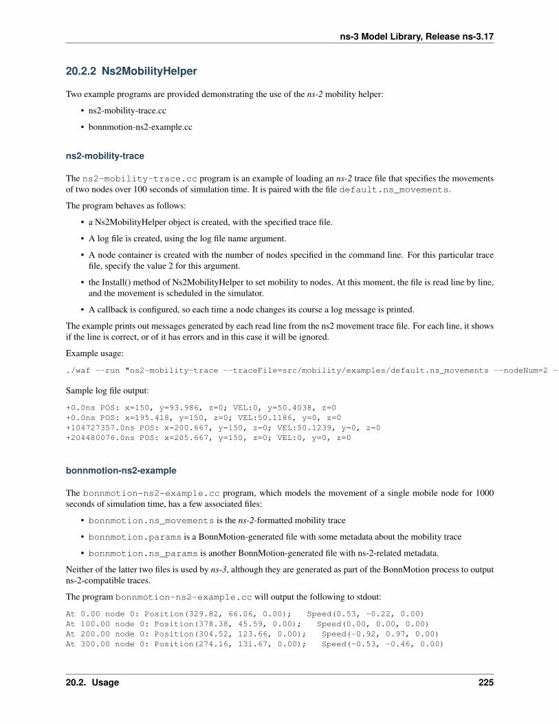
ns-3 Model Library, Release ns-3.17
20.2.2 Ns2MobilityHelper
Two example programs are provided demonstrating the use of the ns-2 mobility helper:
• ns2-mobility-trace.cc
• bonnmotion-ns2-example.cc
ns2-mobility-trace
The ns2-mobility-trace.cc program is an example of loading an ns-2 trace file that specifies the movementsof two nodes over 100 seconds of simulation time. It is paired with the file default.ns_movements.
The program behaves as follows:
• a Ns2MobilityHelper object is created, with the specified trace file.
• A log file is created, using the log file name argument.
• A node container is created with the number of nodes specified in the command line. For this particular tracefile, specify the value 2 for this argument.
• the Install() method of Ns2MobilityHelper to set mobility to nodes. At this moment, the file is read line by line,and the movement is scheduled in the simulator.
• A callback is configured, so each time a node changes its course a log message is printed.
The example prints out messages generated by each read line from the ns2 movement trace file. For each line, it showsif the line is correct, or of it has errors and in this case it will be ignored.
Example usage:
./waf --run "ns2-mobility-trace --traceFile=src/mobility/examples/default.ns_movements --nodeNum=2 --duration=100.0 --logFile=ns2-mob.log"
Sample log file output:
+0.0ns POS: x=150, y=93.986, z=0; VEL:0, y=50.4038, z=0+0.0ns POS: x=195.418, y=150, z=0; VEL:50.1186, y=0, z=0+104727357.0ns POS: x=200.667, y=150, z=0; VEL:50.1239, y=0, z=0+204480076.0ns POS: x=205.667, y=150, z=0; VEL:0, y=0, z=0
bonnmotion-ns2-example
The bonnmotion-ns2-example.cc program, which models the movement of a single mobile node for 1000seconds of simulation time, has a few associated files:
• bonnmotion.ns_movements is the ns-2-formatted mobility trace
• bonnmotion.params is a BonnMotion-generated file with some metadata about the mobility trace
• bonnmotion.ns_params is another BonnMotion-generated file with ns-2-related metadata.
Neither of the latter two files is used by ns-3, although they are generated as part of the BonnMotion process to outputns-2-compatible traces.
The program bonnmotion-ns2-example.cc will output the following to stdout:
At 0.00 node 0: Position(329.82, 66.06, 0.00); Speed(0.53, -0.22, 0.00)At 100.00 node 0: Position(378.38, 45.59, 0.00); Speed(0.00, 0.00, 0.00)At 200.00 node 0: Position(304.52, 123.66, 0.00); Speed(-0.92, 0.97, 0.00)At 300.00 node 0: Position(274.16, 131.67, 0.00); Speed(-0.53, -0.46, 0.00)
20.2. Usage 225
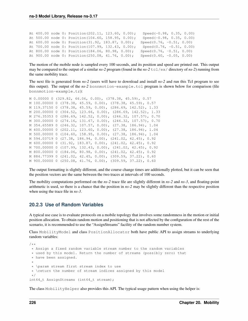
ns-3 Model Library, Release ns-3.17
At 400.00 node 0: Position(202.11, 123.60, 0.00); Speed(-0.98, 0.35, 0.00)At 500.00 node 0: Position(104.60, 158.95, 0.00); Speed(-0.98, 0.35, 0.00)At 600.00 node 0: Position(31.92, 183.87, 0.00); Speed(0.76, -0.51, 0.00)At 700.00 node 0: Position(107.99, 132.43, 0.00); Speed(0.76, -0.51, 0.00)At 800.00 node 0: Position(184.06, 80.98, 0.00); Speed(0.76, -0.51, 0.00)At 900.00 node 0: Position(250.08, 41.76, 0.00); Speed(0.60, -0.05, 0.00)
The motion of the mobile node is sampled every 100 seconds, and its position and speed are printed out. This outputmay be compared to the output of a similar ns-2 program (found in the ns-2 tcl/ex/ directory of ns-2) running fromthe same mobility trace.
The next file is generated from ns-2 (users will have to download and install ns-2 and run this Tcl program to seethis output). The output of the ns-2 bonnmotion-example.tcl program is shown below for comparison (filebonnmotion-example.tr):
M 0.00000 0 (329.82, 66.06, 0.00), (378.38, 45.59), 0.57M 100.00000 0 (378.38, 45.59, 0.00), (378.38, 45.59), 0.57M 119.37150 0 (378.38, 45.59, 0.00), (286.69, 142.52), 1.33M 200.00000 0 (304.52, 123.66, 0.00), (286.69, 142.52), 1.33M 276.35353 0 (286.69, 142.52, 0.00), (246.32, 107.57), 0.70M 300.00000 0 (274.16, 131.67, 0.00), (246.32, 107.57), 0.70M 354.65589 0 (246.32, 107.57, 0.00), (27.38, 186.94), 1.04M 400.00000 0 (202.11, 123.60, 0.00), (27.38, 186.94), 1.04M 500.00000 0 (104.60, 158.95, 0.00), (27.38, 186.94), 1.04M 594.03719 0 (27.38, 186.94, 0.00), (241.02, 42.45), 0.92M 600.00000 0 (31.92, 183.87, 0.00), (241.02, 42.45), 0.92M 700.00000 0 (107.99, 132.43, 0.00), (241.02, 42.45), 0.92M 800.00000 0 (184.06, 80.98, 0.00), (241.02, 42.45), 0.92M 884.77399 0 (241.02, 42.45, 0.00), (309.59, 37.22), 0.60M 900.00000 0 (250.08, 41.76, 0.00), (309.59, 37.22), 0.60
The output formatting is slightly different, and the course change times are additionally plotted, but it can be seen thatthe position vectors are the same between the two traces at intervals of 100 seconds.
The mobility computations performed on the ns-2 trace file are slightly different in ns-2 and ns-3, and floating-pointarithmetic is used, so there is a chance that the position in ns-2 may be slightly different than the respective positionwhen using the trace file in ns-3.
20.2.3 Use of Random Variables
A typical use case is to evaluate protocols on a mobile topology that involves some randomness in the motion or initialposition allocation. To obtain random motion and positioning that is not affected by the configuration of the rest of thescenario, it is recommended to use the “AssignStreams” facility of the random number system.
Class MobilityModel and class PositionAllocator both have public API to assign streams to underlyingrandom variables:
/*** Assign a fixed random variable stream number to the random variables
* used by this model. Return the number of streams (possibly zero) that
* have been assigned.
** \param stream first stream index to use
* \return the number of stream indices assigned by this model
*/int64_t AssignStreams (int64_t stream);
The class MobilityHelper also provides this API. The typical usage pattern when using the helper is:
226 Chapter 20. Mobility
ns-3 Model Library, Release ns-3.17
int64_t streamIndex = /*some positive integer */MobilityHelper mobility;... (configure mobility)mobility.Install (wifiStaNodes);int64_t streamsUsed = mobility.AssignStreams (wifiStaNodes, streamIndex);
If AssignStreams is called before Install, it will not have any effect.
20.2.4 Advanced Usage
A number of external tools can be used to generate traces read by the Ns2MobilityHelper.
ns-2 scengen
TBD
BonnMotion
http://net.cs.uni-bonn.de/wg/cs/applications/bonnmotion/
SUMO
http://sourceforge.net/apps/mediawiki/sumo/index.php?title=Main_Page
TraNS
http://trans.epfl.ch/
20.2.5 Examples
• main-random-topology.cc
• main-random-walk.cc
• main-grid-topology.cc
• ns2-mobility-trace.cc
• ns2-bonnmotion.cc
20.3 Validation
TBD
20.3. Validation 227

ns-3 Model Library, Release ns-3.17
228 Chapter 20. Mobility
CHAPTER
TWENTYONE
NETWORK MODULE
21.1 Packets
The design of the Packet framework of ns was heavily guided by a few important use-cases:
• avoid changing the core of the simulator to introduce new types of packet headers or trailers
• maximize the ease of integration with real-world code and systems
• make it easy to support fragmentation, defragmentation, and, concatenation which are important, especially inwireless systems.
• make memory management of this object efficient
• allow actual application data or dummy application bytes for emulated applications
Each network packet contains a byte buffer, a set of byte tags, a set of packet tags, and metadata.
The byte buffer stores the serialized content of the headers and trailers added to a packet. The serialized representationof these headers is expected to match that of real network packets bit for bit (although nothing forces you to do this)which means that the content of a packet buffer is expected to be that of a real packet.
Fragmentation and defragmentation are quite natural to implement within this context: since we have a buffer of realbytes, we can split it in multiple fragments and re-assemble these fragments. We expect that this choice will make itreally easy to wrap our Packet data structure within Linux-style skb or BSD-style mbuf to integrate real-world kernelcode in the simulator. We also expect that performing a real-time plug of the simulator to a real-world network will beeasy.
One problem that this design choice raises is that it is difficult to pretty-print the packet headers without context. Thepacket metadata describes the type of the headers and trailers which were serialized in the byte buffer. The maintenanceof metadata is optional and disabled by default. To enable it, you must call Packet::EnableMetadata() and this willallow you to get non-empty output from Packet::Print and Packet::Print.
Also, developers often want to store data in packet objects that is not found in the real packets (such as timestamps orflow-ids). The Packet class deals with this requirement by storing a set of tags (class Tag). We have found two classesof use cases for these tags, which leads to two different types of tags. So-called ‘byte’ tags are used to tag a subset ofthe bytes in the packet byte buffer while ‘packet’ tags are used to tag the packet itself. The main difference betweenthese two kinds of tags is what happens when packets are copied, fragmented, and reassembled: ‘byte’ tags followbytes while ‘packet’ tags follow packets. Another important difference between these two kinds of tags is that bytetags cannot be removed and are expected to be written once, and read many times, while packet tags are expected to bewritten once, read many times, and removed exactly once. An example of a ‘byte’ tag is a FlowIdTag which containsa flow id and is set by the application generating traffic. An example of a ‘packet’ tag is a cross-layer QoS class id setby an application and processed by a lower-level MAC layer.
Memory management of Packet objects is entirely automatic and extremely efficient: memory for the application-levelpayload can be modeled by a virtual buffer of zero-filled bytes for which memory is never allocated unless explicitly
229
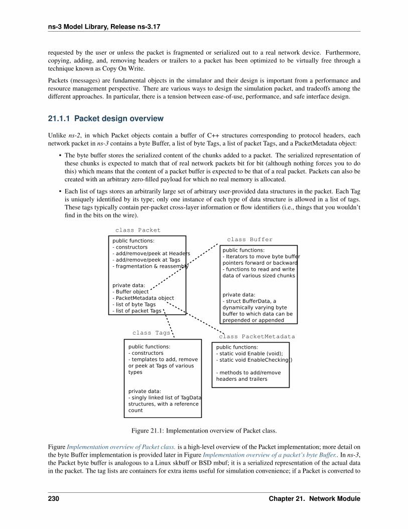
ns-3 Model Library, Release ns-3.17
requested by the user or unless the packet is fragmented or serialized out to a real network device. Furthermore,copying, adding, and, removing headers or trailers to a packet has been optimized to be virtually free through atechnique known as Copy On Write.
Packets (messages) are fundamental objects in the simulator and their design is important from a performance andresource management perspective. There are various ways to design the simulation packet, and tradeoffs among thedifferent approaches. In particular, there is a tension between ease-of-use, performance, and safe interface design.
21.1.1 Packet design overview
Unlike ns-2, in which Packet objects contain a buffer of C++ structures corresponding to protocol headers, eachnetwork packet in ns-3 contains a byte Buffer, a list of byte Tags, a list of packet Tags, and a PacketMetadata object:
• The byte buffer stores the serialized content of the chunks added to a packet. The serialized representation ofthese chunks is expected to match that of real network packets bit for bit (although nothing forces you to dothis) which means that the content of a packet buffer is expected to be that of a real packet. Packets can also becreated with an arbitrary zero-filled payload for which no real memory is allocated.
• Each list of tags stores an arbitrarily large set of arbitrary user-provided data structures in the packet. Each Tagis uniquely identified by its type; only one instance of each type of data structure is allowed in a list of tags.These tags typically contain per-packet cross-layer information or flow identifiers (i.e., things that you wouldn’tfind in the bits on the wire).
Figure 21.1: Implementation overview of Packet class.
Figure Implementation overview of Packet class. is a high-level overview of the Packet implementation; more detail onthe byte Buffer implementation is provided later in Figure Implementation overview of a packet’s byte Buffer.. In ns-3,the Packet byte buffer is analogous to a Linux skbuff or BSD mbuf; it is a serialized representation of the actual datain the packet. The tag lists are containers for extra items useful for simulation convenience; if a Packet is converted to
230 Chapter 21. Network Module
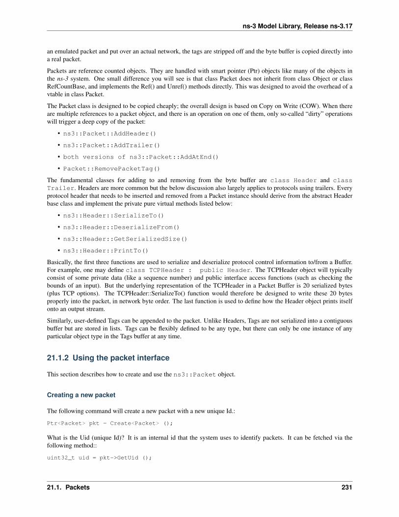
ns-3 Model Library, Release ns-3.17
an emulated packet and put over an actual network, the tags are stripped off and the byte buffer is copied directly intoa real packet.
Packets are reference counted objects. They are handled with smart pointer (Ptr) objects like many of the objects inthe ns-3 system. One small difference you will see is that class Packet does not inherit from class Object or classRefCountBase, and implements the Ref() and Unref() methods directly. This was designed to avoid the overhead of avtable in class Packet.
The Packet class is designed to be copied cheaply; the overall design is based on Copy on Write (COW). When thereare multiple references to a packet object, and there is an operation on one of them, only so-called “dirty” operationswill trigger a deep copy of the packet:
• ns3::Packet::AddHeader()
• ns3::Packet::AddTrailer()
• both versions of ns3::Packet::AddAtEnd()
• Packet::RemovePacketTag()
The fundamental classes for adding to and removing from the byte buffer are class Header and classTrailer. Headers are more common but the below discussion also largely applies to protocols using trailers. Everyprotocol header that needs to be inserted and removed from a Packet instance should derive from the abstract Headerbase class and implement the private pure virtual methods listed below:
• ns3::Header::SerializeTo()
• ns3::Header::DeserializeFrom()
• ns3::Header::GetSerializedSize()
• ns3::Header::PrintTo()
Basically, the first three functions are used to serialize and deserialize protocol control information to/from a Buffer.For example, one may define class TCPHeader : public Header. The TCPHeader object will typicallyconsist of some private data (like a sequence number) and public interface access functions (such as checking thebounds of an input). But the underlying representation of the TCPHeader in a Packet Buffer is 20 serialized bytes(plus TCP options). The TCPHeader::SerializeTo() function would therefore be designed to write these 20 bytesproperly into the packet, in network byte order. The last function is used to define how the Header object prints itselfonto an output stream.
Similarly, user-defined Tags can be appended to the packet. Unlike Headers, Tags are not serialized into a contiguousbuffer but are stored in lists. Tags can be flexibly defined to be any type, but there can only be one instance of anyparticular object type in the Tags buffer at any time.
21.1.2 Using the packet interface
This section describes how to create and use the ns3::Packet object.
Creating a new packet
The following command will create a new packet with a new unique Id.:
Ptr<Packet> pkt = Create<Packet> ();
What is the Uid (unique Id)? It is an internal id that the system uses to identify packets. It can be fetched via thefollowing method::
uint32_t uid = pkt->GetUid ();
21.1. Packets 231
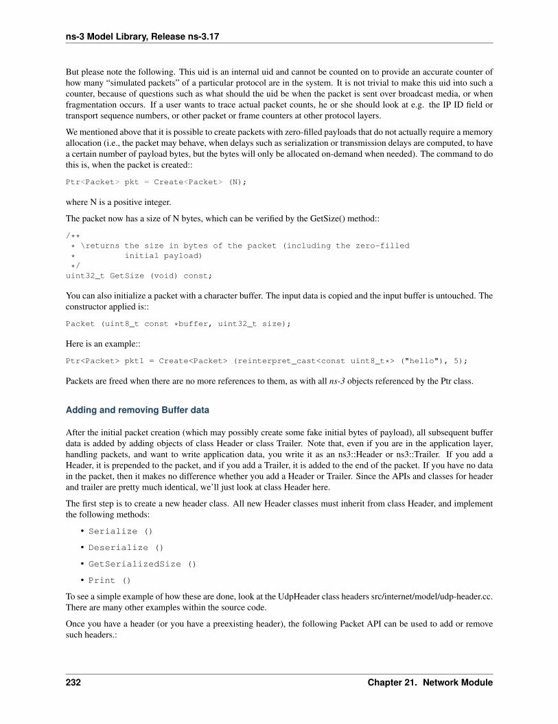
ns-3 Model Library, Release ns-3.17
But please note the following. This uid is an internal uid and cannot be counted on to provide an accurate counter ofhow many “simulated packets” of a particular protocol are in the system. It is not trivial to make this uid into such acounter, because of questions such as what should the uid be when the packet is sent over broadcast media, or whenfragmentation occurs. If a user wants to trace actual packet counts, he or she should look at e.g. the IP ID field ortransport sequence numbers, or other packet or frame counters at other protocol layers.
We mentioned above that it is possible to create packets with zero-filled payloads that do not actually require a memoryallocation (i.e., the packet may behave, when delays such as serialization or transmission delays are computed, to havea certain number of payload bytes, but the bytes will only be allocated on-demand when needed). The command to dothis is, when the packet is created::
Ptr<Packet> pkt = Create<Packet> (N);
where N is a positive integer.
The packet now has a size of N bytes, which can be verified by the GetSize() method::
/*** \returns the size in bytes of the packet (including the zero-filled
* initial payload)
*/uint32_t GetSize (void) const;
You can also initialize a packet with a character buffer. The input data is copied and the input buffer is untouched. Theconstructor applied is::
Packet (uint8_t const *buffer, uint32_t size);
Here is an example::
Ptr<Packet> pkt1 = Create<Packet> (reinterpret_cast<const uint8_t*> ("hello"), 5);
Packets are freed when there are no more references to them, as with all ns-3 objects referenced by the Ptr class.
Adding and removing Buffer data
After the initial packet creation (which may possibly create some fake initial bytes of payload), all subsequent bufferdata is added by adding objects of class Header or class Trailer. Note that, even if you are in the application layer,handling packets, and want to write application data, you write it as an ns3::Header or ns3::Trailer. If you add aHeader, it is prepended to the packet, and if you add a Trailer, it is added to the end of the packet. If you have no datain the packet, then it makes no difference whether you add a Header or Trailer. Since the APIs and classes for headerand trailer are pretty much identical, we’ll just look at class Header here.
The first step is to create a new header class. All new Header classes must inherit from class Header, and implementthe following methods:
• Serialize ()
• Deserialize ()
• GetSerializedSize ()
• Print ()
To see a simple example of how these are done, look at the UdpHeader class headers src/internet/model/udp-header.cc.There are many other examples within the source code.
Once you have a header (or you have a preexisting header), the following Packet API can be used to add or removesuch headers.:
232 Chapter 21. Network Module
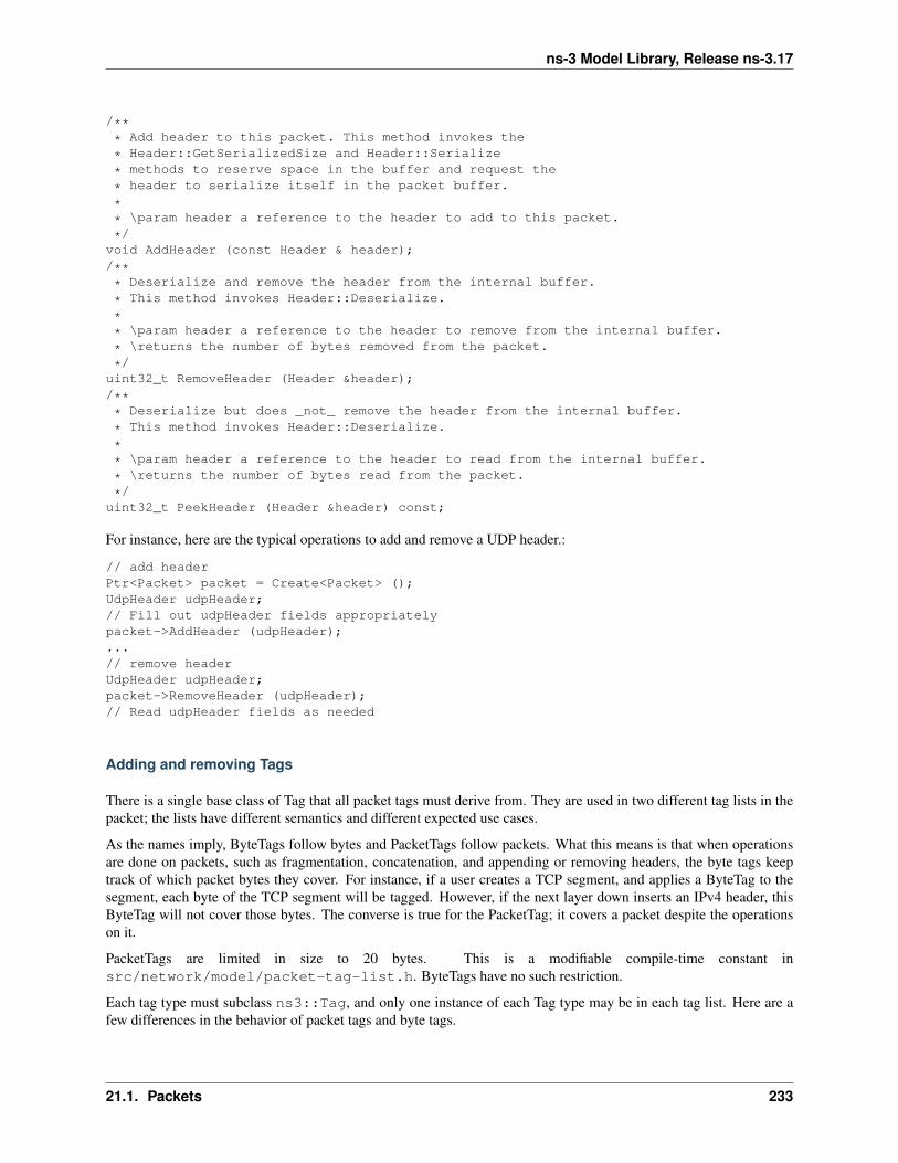
ns-3 Model Library, Release ns-3.17
/*** Add header to this packet. This method invokes the
* Header::GetSerializedSize and Header::Serialize
* methods to reserve space in the buffer and request the
* header to serialize itself in the packet buffer.
** \param header a reference to the header to add to this packet.
*/void AddHeader (const Header & header);/*** Deserialize and remove the header from the internal buffer.
* This method invokes Header::Deserialize.
** \param header a reference to the header to remove from the internal buffer.
* \returns the number of bytes removed from the packet.
*/uint32_t RemoveHeader (Header &header);/*** Deserialize but does _not_ remove the header from the internal buffer.
* This method invokes Header::Deserialize.
** \param header a reference to the header to read from the internal buffer.
* \returns the number of bytes read from the packet.
*/uint32_t PeekHeader (Header &header) const;
For instance, here are the typical operations to add and remove a UDP header.:
// add headerPtr<Packet> packet = Create<Packet> ();UdpHeader udpHeader;// Fill out udpHeader fields appropriatelypacket->AddHeader (udpHeader);...// remove headerUdpHeader udpHeader;packet->RemoveHeader (udpHeader);// Read udpHeader fields as needed
Adding and removing Tags
There is a single base class of Tag that all packet tags must derive from. They are used in two different tag lists in thepacket; the lists have different semantics and different expected use cases.
As the names imply, ByteTags follow bytes and PacketTags follow packets. What this means is that when operationsare done on packets, such as fragmentation, concatenation, and appending or removing headers, the byte tags keeptrack of which packet bytes they cover. For instance, if a user creates a TCP segment, and applies a ByteTag to thesegment, each byte of the TCP segment will be tagged. However, if the next layer down inserts an IPv4 header, thisByteTag will not cover those bytes. The converse is true for the PacketTag; it covers a packet despite the operationson it.
PacketTags are limited in size to 20 bytes. This is a modifiable compile-time constant insrc/network/model/packet-tag-list.h. ByteTags have no such restriction.
Each tag type must subclass ns3::Tag, and only one instance of each Tag type may be in each tag list. Here are afew differences in the behavior of packet tags and byte tags.
21.1. Packets 233
ns-3 Model Library, Release ns-3.17
• Fragmentation: As mentioned above, when a packet is fragmented, each packet fragment (which is a newpacket) will get a copy of all packet tags, and byte tags will follow the new packet boundaries (i.e. if thefragmented packets fragment across a buffer region covered by the byte tag, both packet fragments will stillhave the appropriate buffer regions byte tagged).
• Concatenation: When packets are combined, two different buffer regions will become one. For byte tags, thebyte tags simply follow the respective buffer regions. For packet tags, only the tags on the first packet survivethe merge.
• Finding and Printing: Both classes allow you to iterate over all of the tags and print them.
• Removal: Users can add and remove the same packet tag multiple times on a single packet (AddPacketTag ()and RemovePacketTag ()). The packet However, once a byte tag is added, it can only be removed by strippingall byte tags from the packet. Removing one of possibly multiple byte tags is not supported by the current API.
As of ns-3.5 and later, Tags are not serialized and deserialized to a buffer when Packet::Serialize () andPacket::Deserialize () are called; this is an open bug.
If a user wants to take an existing packet object and reuse it as a new packet, he or she should remove all byte tags andpacket tags before doing so. An example is the UdpEchoServer class, which takes the received packet and “turns itaround” to send back to the echo client.
The Packet API for byte tags is given below.:
/*** \param tag the new tag to add to this packet
** Tag each byte included in this packet with the
* new tag.
** Note that adding a tag is a const operation which is pretty
* un-intuitive. The rationale is that the content and behavior of
* a packet is _not_ changed when a tag is added to a packet: any
* code which was not aware of the new tag is going to work just
* the same if the new tag is added. The real reason why adding a
* tag was made a const operation is to allow a trace sink which gets
* a packet to tag the packet, even if the packet is const (and most
* trace sources should use const packets because it would be
* totally evil to allow a trace sink to modify the content of a
* packet).
*/void AddByteTag (const Tag &tag) const;/*** \returns an iterator over the set of byte tags included in this packet.
*/ByteTagIterator GetByteTagIterator (void) const;/*** \param tag the tag to search in this packet
* \returns true if the requested tag type was found, false otherwise.
** If the requested tag type is found, it is copied in the user’s
* provided tag instance.
*/bool FindFirstMatchingByteTag (Tag &tag) const;
/*** Remove all the tags stored in this packet.
*/void RemoveAllByteTags (void);
234 Chapter 21. Network Module
ns-3 Model Library, Release ns-3.17
/*** \param os output stream in which the data should be printed.
** Iterate over the tags present in this packet, and
* invoke the Print method of each tag stored in the packet.
*/void PrintByteTags (std::ostream &os) const;
The Packet API for packet tags is given below.:
/*** \param tag the tag to store in this packet
** Add a tag to this packet. This method calls the
* Tag::GetSerializedSize and, then, Tag::Serialize.
** Note that this method is const, that is, it does not
* modify the state of this packet, which is fairly
* un-intuitive.
*/void AddPacketTag (const Tag &tag) const;/*** \param tag the tag to remove from this packet
* \returns true if the requested tag is found, false
* otherwise.
** Remove a tag from this packet. This method calls
* Tag::Deserialize if the tag is found.
*/bool RemovePacketTag (Tag &tag);/*** \param tag the tag to search in this packet
* \returns true if the requested tag is found, false
* otherwise.
** Search a matching tag and call Tag::Deserialize if it is found.
*/bool PeekPacketTag (Tag &tag) const;/*** Remove all packet tags.
*/void RemoveAllPacketTags (void);
/*** \param os the stream in which we want to print data.
** Print the list of ’packet’ tags.
** \sa Packet::AddPacketTag, Packet::RemovePacketTag, Packet::PeekPacketTag,
* Packet::RemoveAllPacketTags
*/void PrintPacketTags (std::ostream &os) const;
/*** \returns an object which can be used to iterate over the list of
* packet tags.
*/PacketTagIterator GetPacketTagIterator (void) const;
21.1. Packets 235
ns-3 Model Library, Release ns-3.17
Here is a simple example illustrating the use of tags from the code insrc/internet/model/udp-socket-impl.cc::
Ptr<Packet> p; // pointer to a pre-existing packetSocketIpTtlTag tagtag.SetTtl (m_ipMulticastTtl); // Convey the TTL from UDP layer to IP layerp->AddPacketTag (tag);
This tag is read at the IP layer, then stripped (src/internet/model/ipv4-l3-protocol.cc)::
uint8_t ttl = m_defaultTtl;SocketIpTtlTag tag;bool found = packet->RemovePacketTag (tag);if (found)
{ttl = tag.GetTtl ();
}
Fragmentation and concatenation
Packets may be fragmented or merged together. For example, to fragment a packet p of 90 bytes into two packets, onecontaining the first 10 bytes and the other containing the remaining 80, one may call the following code::
Ptr<Packet> frag0 = p->CreateFragment (0, 10);Ptr<Packet> frag1 = p->CreateFragment (10, 90);
As discussed above, the packet tags from p will follow to both packet fragments, and the byte tags will follow the byteranges as needed.
Now, to put them back together::
frag0->AddAtEnd (frag1);
Now frag0 should be equivalent to the original packet p. If, however, there were operations on the fragments beforebeing reassembled (such as tag operations or header operations), the new packet will not be the same.
Enabling metadata
We mentioned above that packets, being on-the-wire representations of byte buffers, present a problem to print outin a structured way unless the printing function has access to the context of the header. For instance, consider atcpdump-like printer that wants to pretty-print the contents of a packet.
To enable this usage, packets may have metadata enabled (disabled by default for performance reasons). This class isused by the Packet class to record every operation performed on the packet’s buffer, and provides an implementationof Packet::Print () method that uses the metadata to analyze the content of the packet’s buffer.
The metadata is also used to perform extensive sanity checks at runtime when performing operations on a Packet. Forexample, this metadata is used to verify that when you remove a header from a packet, this same header was actuallypresent at the front of the packet. These errors will be detected and will abort the program.
To enable this operation, users will typically insert one or both of these statements at the beginning of their programs::
Packet::EnablePrinting ();Packet::EnableChecking ();
236 Chapter 21. Network Module
ns-3 Model Library, Release ns-3.17
21.1.3 Sample programs
See src/network/examples/main-packet-header.cc and src/network/examples/main-packet-tag.cc.
21.1.4 Implementation details
Private member variables
A Packet object’s interface provides access to some private data::
Buffer m_buffer;ByteTagList m_byteTagList;PacketTagList m_packetTagList;PacketMetadata m_metadata;mutable uint32_t m_refCount;static uint32_t m_globalUid;
Each Packet has a Buffer and two Tags lists, a PacketMetadata object, and a ref count. A static member variable keepstrack of the UIDs allocated. The actual uid of the packet is stored in the PacketMetadata.
Note: that real network packets do not have a UID; the UID is therefore an instance of data that normally would bestored as a Tag in the packet. However, it was felt that a UID is a special case that is so often used in simulations thatit would be more convenient to store it in a member variable.
Buffer implementation
Class Buffer represents a buffer of bytes. Its size is automatically adjusted to hold any data prepended or appendedby the user. Its implementation is optimized to ensure that the number of buffer resizes is minimized, by creating newBuffers of the maximum size ever used. The correct maximum size is learned at runtime during use by recording themaximum size of each packet.
Authors of new Header or Trailer classes need to know the public API of the Buffer class. (add summary here)
The byte buffer is implemented as follows:
struct BufferData {uint32_t m_count;uint32_t m_size;uint32_t m_initialStart;uint32_t m_dirtyStart;uint32_t m_dirtySize;uint8_t m_data[1];
};struct BufferData *m_data;uint32_t m_zeroAreaSize;uint32_t m_start;uint32_t m_size;
• BufferData::m_count: reference count for BufferData structure
• BufferData::m_size: size of data buffer stored in BufferData structure
• BufferData::m_initialStart: offset from start of data buffer where data was first inserted
• BufferData::m_dirtyStart: offset from start of buffer where every Buffer which holds a reference tothis BufferData instance have written data so far
• BufferData::m_dirtySize: size of area where data has been written so far
21.1. Packets 237
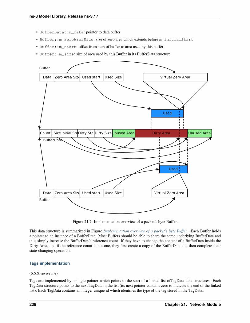
ns-3 Model Library, Release ns-3.17
• BufferData::m_data: pointer to data buffer
• Buffer::m_zeroAreaSize: size of zero area which extends before m_initialStart
• Buffer::m_start: offset from start of buffer to area used by this buffer
• Buffer::m_size: size of area used by this Buffer in its BufferData structure
Figure 21.2: Implementation overview of a packet’s byte Buffer.
This data structure is summarized in Figure Implementation overview of a packet’s byte Buffer.. Each Buffer holdsa pointer to an instance of a BufferData. Most Buffers should be able to share the same underlying BufferData andthus simply increase the BufferData’s reference count. If they have to change the content of a BufferData inside theDirty Area, and if the reference count is not one, they first create a copy of the BufferData and then complete theirstate-changing operation.
Tags implementation
(XXX revise me)
Tags are implemented by a single pointer which points to the start of a linked list ofTagData data structures. EachTagData structure points to the next TagData in the list (its next pointer contains zero to indicate the end of the linkedlist). Each TagData contains an integer unique id which identifies the type of the tag stored in the TagData.:
238 Chapter 21. Network Module
ns-3 Model Library, Release ns-3.17
struct TagData {struct TagData *m_next;uint32_t m_id;uint32_t m_count;uint8_t m_data[Tags::SIZE];
};class Tags {
struct TagData *m_next;};
Adding a tag is a matter of inserting a new TagData at the head of the linked list. Looking at a tag requires you to findthe relevant TagData in the linked list and copy its data into the user data structure. Removing a tag and updating thecontent of a tag requires a deep copy of the linked list before performing this operation. On the other hand, copying aPacket and its tags is a matter of copying the TagData head pointer and incrementing its reference count.
Tags are found by the unique mapping between the Tag type and its underlying id. This is why at most one instanceof any Tag can be stored in a packet. The mapping between Tag type and underlying id is performed by a registrationas follows::
/* A sample Tag implementation
*/struct MyTag {
uint16_t m_streamId;};
Memory management
Describe dataless vs. data-full packets.
Copy-on-write semantics
The current implementation of the byte buffers and tag list is based on COW (Copy On Write). An introduction toCOW can be found in Scott Meyer’s “More Effective C++”, items 17 and 29). This design feature and aspects ofthe public interface borrows from the packet design of the Georgia Tech Network Simulator. This implementation ofCOW uses a customized reference counting smart pointer class.
What COW means is that copying packets without modifying them is very cheap (in terms of CPU and memory usage)and modifying them can be also very cheap. What is key for proper COW implementations is being able to detectwhen a given modification of the state of a packet triggers a full copy of the data prior to the modification: COWsystems need to detect when an operation is “dirty” and must therefore invoke a true copy.
Dirty operations:
• ns3::Packet::AddHeader
• ns3::Packet::AddTrailer
• both versions of ns3::Packet::AddAtEnd
• ns3::Packet::RemovePacketTag
Non-dirty operations:
• ns3::Packet::AddPacketTag
• ns3::Packet::PeekPacketTag
• ns3::Packet::RemoveAllPacketTags
• ns3::Packet::AddByteTag
21.1. Packets 239
ns-3 Model Library, Release ns-3.17
• ns3::Packet::FindFirstMatchingByteTag
• ns3::Packet::RemoveAllByteTags
• ns3::Packet::RemoveHeader
• ns3::Packet::RemoveTrailer
• ns3::Packet::CreateFragment
• ns3::Packet::RemoveAtStart
• ns3::Packet::RemoveAtEnd
• ns3::Packet::CopyData
Dirty operations will always be slower than non-dirty operations, sometimes by several orders of magnitude. How-ever, even the dirty operations have been optimized for common use-cases which means that most of the time, theseoperations will not trigger data copies and will thus be still very fast.
21.2 Error Model
This section documents a few error model objects, typically associated with NetDevice models, that are maintained aspart of the network module:
• RateErrorModel
• ListErrorModel
• ReceiveListErrorModel
• BurstErrorModel
Error models are used to indicate that a packet should be considered to be errored, according to the underlying (possiblystochastic or empirical) error model.
21.2.1 Model Description
The source code for error models live in the directory src/packet/utils.
Two types of error models are generally provided. The first are stochastic models. In this case, packets are erroredaccording to underlying random variable distributions. An example of this is the RateErrorModel. The othertype of model is a deterministic or empirical model, in which packets are errored according to a particular prescribedpattern. An example is the ListErrorModel that allows users to specify the list of packets to be errored, by listingthe specific packet UIDs.
The ns3::RateErrorModel errors packets according to an underlying random variable distribution, which is bydefault a UniformRandomVariable distributed between 0.0 and 1.0. The error rate and error units (bit, byte, or packet)are set by the user. For instance, by setting ErrorRate to 0.1 and ErrorUnit to “Packet”, in the long run, around 10% ofthe packets will be lost.
Design
Error models are ns-3 objects and can be created using the typical pattern of CreateObject<>(). They haveconfiguration attributes.
An ErrorModel can be applied anywhere, but are commonly deployed on NetDevice models so that artificial losses(mimicing channel losses) can be induced.
240 Chapter 21. Network Module
ns-3 Model Library, Release ns-3.17
Scope and Limitations
No known limitations. There are no existing models that try to modify the packet contents (e.g. apply bit or byte errorsto the byte buffers). This type of operation will likely be performance-expensive, and existing Packet APIs may noteasily support it.
The ns-3 spectrum model and devices that derive from it (e.g. LTE) have their own error model base class, found in
References
The initial ns-3 error models were ported from ns-2 (queue/errmodel.{cc,h})
21.2.2 Usage
The base class API is as follows:
• bool ErrorModel::IsCorrupt (Ptr<Packet> pkt): Evaluate the packet and return true or falsewhether the packet should be considered errored or not. Some models could potentially alter the contents of thepacket bit buffer.
• void ErrorModel::Reset (void): Reset any state.
• void ErrorModel::Enable (void): Enable the model
• void ErrorModel::Disble (void): Disable the model; IsCorrupt() will always return false.
• bool ErrorModel::IsEnabled (void) const: Return the enabled state
Many ns-3 NetDevices contain attributes holding pointers to error models. The error model is applied in the notionalphysical layer processing chain of the device, and drops should show up on the PhyRxDrop trace source of thedevice. The following are known to include an attribute with a pointer available to hold this type of error model:
• SimpleNetDevice
• PointToPointNetDevice
• CsmaNetDevice
• VirtualNetDevice
However, the ErrorModel could be used anywhere where packets are used
Helpers
This model is typically not used with helpers.
Attributes
The RateErrorModel contains the following attributes:
Output
What kind of data does the model generate? What are the key trace sources? What kind of logging output can beenabled?
21.2. Error Model 241
ns-3 Model Library, Release ns-3.17
Examples
Error models are used in the tutorial fifth and sixth programs.
The directory examples/error-model/ contains an example simple-error-model.cc that exercises theRate and List error models.
The TCP example examples/tcp/tcp-nsc-lfn.cc uses the Rate error model.
Troubleshooting
No known issues.
21.2.3 Validation
The error-model unit test suite provides a single test case of of a particular combination of ErrorRate and ErrorUnitfor the RateErrorModel applied to a SimpleNetDevice.
21.2.4 Acknowledgements
The basic ErrorModel, RateErrorModel, and ListErrorModel classes were ported from ns-2 to ns-3 in 2007. TheReceiveListErrorModel was added at that time.
The burst error model is due to Truc Anh N. Nguyen at the University of Kansas (James P.G. Sterbenz<[email protected]>, director, ResiliNets Research Group (http://wiki.ittc.ku.edu/resilinets), Information and Telecom-munication Technology Center (ITTC) and Department of Electrical Engineering and Computer Science, The Univer-sity of Kansas Lawrence, KS USA). Work supported in part by NSF FIND (Future Internet Design) Program undergrant CNS-0626918 (Postmodern Internet Architecture), NSF grant CNS-1050226 (Multilayer Network ResilienceAnalysis and Experimentation on GENI), US Department of Defense (DoD), and ITTC at The University of Kansas.
21.3 Node and NetDevices Overview
This chapter describes how ns-3 nodes are put together, and provides a walk-through of how packets traverse aninternet-based Node.
In ns-3, nodes are instances of ns3::Node. This class may be subclassed, but instead, the conceptual model is thatwe aggregate or insert objects to it rather than define subclasses.
One might think of a bare ns-3 node as a shell of a computer, to which one may add NetDevices (cards) and otherinnards including the protocols and applications. High-level node architecture illustrates that ns3::Node objectscontain a list of ns3::Application instances (initially, the list is empty), a list of ns3::NetDevice instances(initially, the list is empty), a list of ns3::Node::ProtocolHandler instances, a unique integer ID, and a systemID (for distributed simulation).
The design tries to avoid putting too many dependencies on the class ns3::Node, ns3::Application, orns3::NetDevice for the following:
• IP version, or whether IP is at all even used in the ns3::Node.
• implementation details of the IP stack.
From a software perspective, the lower interface of applications corresponds to the C-based sockets API. The upper in-terface of ns3::NetDevice objects corresponds to the device independent sublayer of the Linux stack. Everythingin between can be aggregated and plumbed together as needed.
242 Chapter 21. Network Module
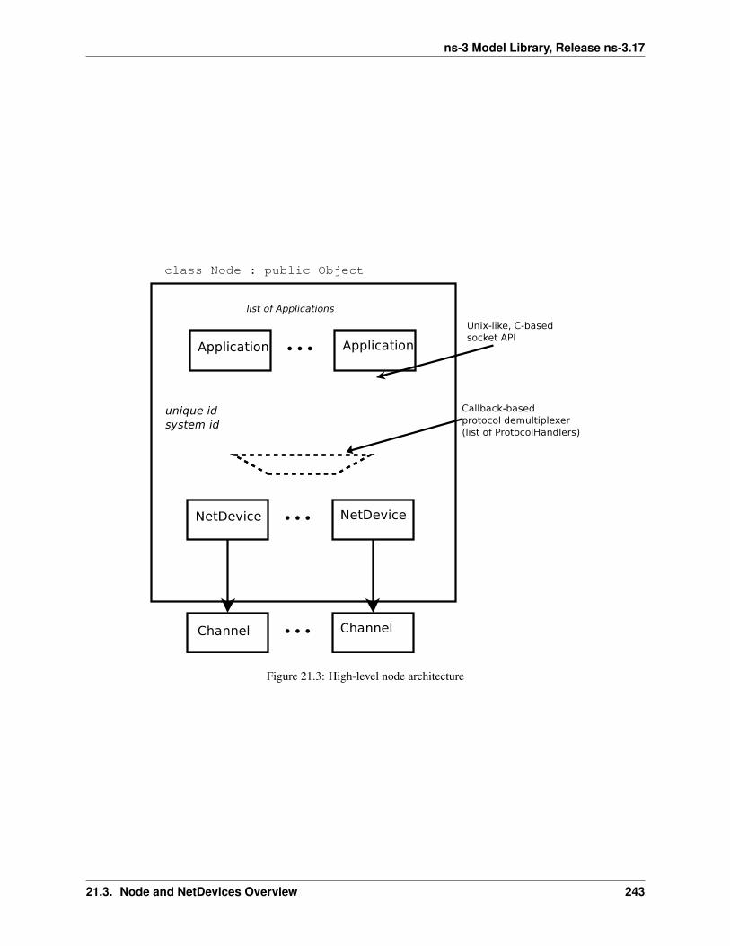
ns-3 Model Library, Release ns-3.17
Figure 21.3: High-level node architecture
21.3. Node and NetDevices Overview 243
ns-3 Model Library, Release ns-3.17
Let’s look more closely at the protocol demultiplexer. We want incoming frames at layer-2 to be delivered to the rightlayer-3 protocol such as IPv4. The function of this demultiplexer is to register callbacks for receiving packets. Thecallbacks are indexed based on the EtherType in the layer-2 frame.
Many different types of higher-layer protocols may be connected to the NetDevice, such as IPv4, IPv6, ARP, MPLS,IEEE 802.1x, and packet sockets. Therefore, the use of a callback-based demultiplexer avoids the need to use acommon base class for all of these protocols, which is problematic because of the different types of objects (includingpacket sockets) expected to be registered there.
21.4 Sockets APIs
The sockets API is a long-standing API used by user-space applications to access network services in the kernel. Asocket is an abstraction, like a Unix file handle, that allows applications to connect to other Internet hosts and exchangereliable byte streams and unreliable datagrams, among other services.
ns-3 provides two types of sockets APIs, and it is important to understand the differences between them. The first is anative ns-3 API, while the second uses the services of the native API to provide a POSIX-like API as part of an overallapplication process. Both APIs strive to be close to the typical sockets API that application writers on Unix systemsare accustomed to, but the POSIX variant is much closer to a real system’s sockets API.
21.4.1 ns-3 sockets API
The native sockets API for ns-3 provides an interface to various types of transport protocols (TCP, UDP) as well as topacket sockets and, in the future, Netlink-like sockets. However, users are cautioned to understand that the semanticsare not the exact same as one finds in a real system (for an API which is very much aligned to real systems, see thenext section).
ns3::Socket is defined in src/network/model/socket.h. Readers will note that many public memberfunctions are aligned with real sockets function calls, and all other things being equal, we have tried to align with aPosix sockets API. However, note that:
• ns-3 applications handle a smart pointer to a Socket object, not a file descriptor;
• there is no notion of synchronous API or a blocking API; in fact, the model for interaction between applicationand socket is one of asynchronous I/O, which is not typically found in real systems (more on this below);
• the C-style socket address structures are not used;
• the API is not a complete sockets API, such as supporting all socket options or all function variants;
• many calls use ns3::Packet class to transfer data between application and socket. This may seem peculiarto pass Packets across a stream socket API, but think of these packets as just fancy byte buffers at this level(more on this also below).
Basic operation and calls
Creating sockets
An application that wants to use sockets must first create one. On real systems using a C-based API, this is accom-plished by calling socket()
int socket(int domain, int type, int protocol);
244 Chapter 21. Network Module
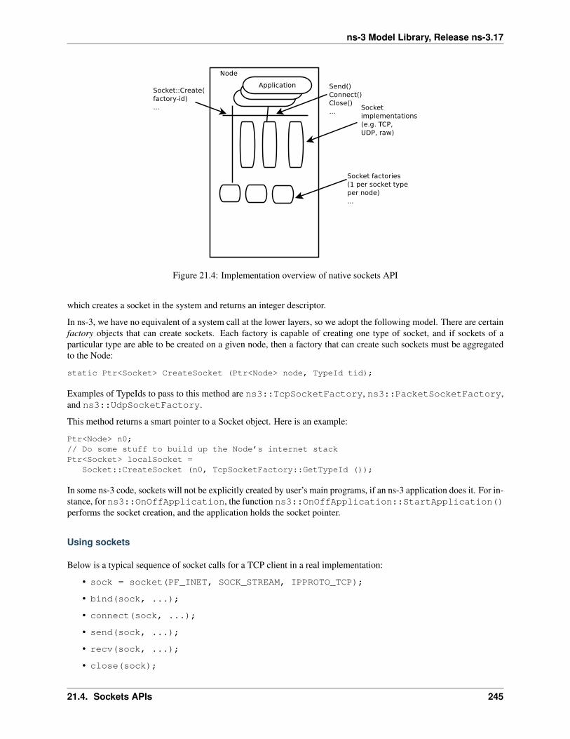
ns-3 Model Library, Release ns-3.17
Figure 21.4: Implementation overview of native sockets API
which creates a socket in the system and returns an integer descriptor.
In ns-3, we have no equivalent of a system call at the lower layers, so we adopt the following model. There are certainfactory objects that can create sockets. Each factory is capable of creating one type of socket, and if sockets of aparticular type are able to be created on a given node, then a factory that can create such sockets must be aggregatedto the Node:
static Ptr<Socket> CreateSocket (Ptr<Node> node, TypeId tid);
Examples of TypeIds to pass to this method are ns3::TcpSocketFactory, ns3::PacketSocketFactory,and ns3::UdpSocketFactory.
This method returns a smart pointer to a Socket object. Here is an example:
Ptr<Node> n0;// Do some stuff to build up the Node’s internet stackPtr<Socket> localSocket =
Socket::CreateSocket (n0, TcpSocketFactory::GetTypeId ());
In some ns-3 code, sockets will not be explicitly created by user’s main programs, if an ns-3 application does it. For in-stance, for ns3::OnOffApplication, the function ns3::OnOffApplication::StartApplication()performs the socket creation, and the application holds the socket pointer.
Using sockets
Below is a typical sequence of socket calls for a TCP client in a real implementation:
• sock = socket(PF_INET, SOCK_STREAM, IPPROTO_TCP);
• bind(sock, ...);
• connect(sock, ...);
• send(sock, ...);
• recv(sock, ...);
• close(sock);
21.4. Sockets APIs 245
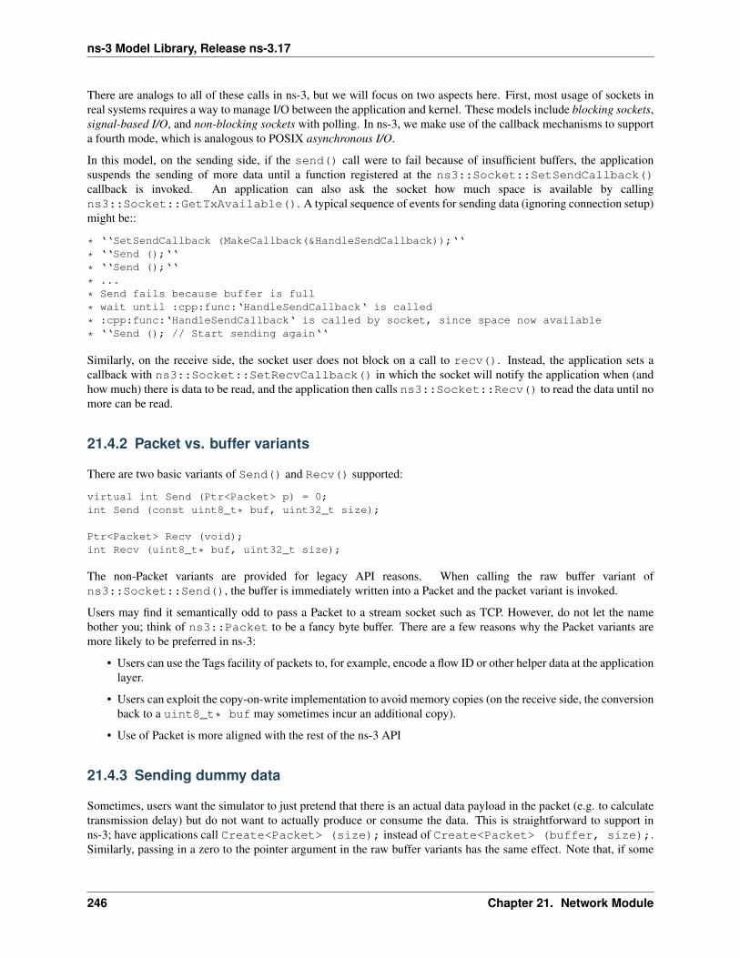
ns-3 Model Library, Release ns-3.17
There are analogs to all of these calls in ns-3, but we will focus on two aspects here. First, most usage of sockets inreal systems requires a way to manage I/O between the application and kernel. These models include blocking sockets,signal-based I/O, and non-blocking sockets with polling. In ns-3, we make use of the callback mechanisms to supporta fourth mode, which is analogous to POSIX asynchronous I/O.
In this model, on the sending side, if the send() call were to fail because of insufficient buffers, the applicationsuspends the sending of more data until a function registered at the ns3::Socket::SetSendCallback()callback is invoked. An application can also ask the socket how much space is available by callingns3::Socket::GetTxAvailable(). A typical sequence of events for sending data (ignoring connection setup)might be::
* ‘‘SetSendCallback (MakeCallback(&HandleSendCallback));‘‘
* ‘‘Send ();‘‘
* ‘‘Send ();‘‘
* ...
* Send fails because buffer is full
* wait until :cpp:func:‘HandleSendCallback‘ is called
* :cpp:func:‘HandleSendCallback‘ is called by socket, since space now available
* ‘‘Send (); // Start sending again‘‘
Similarly, on the receive side, the socket user does not block on a call to recv(). Instead, the application sets acallback with ns3::Socket::SetRecvCallback() in which the socket will notify the application when (andhow much) there is data to be read, and the application then calls ns3::Socket::Recv() to read the data until nomore can be read.
21.4.2 Packet vs. buffer variants
There are two basic variants of Send() and Recv() supported:
virtual int Send (Ptr<Packet> p) = 0;int Send (const uint8_t* buf, uint32_t size);
Ptr<Packet> Recv (void);int Recv (uint8_t* buf, uint32_t size);
The non-Packet variants are provided for legacy API reasons. When calling the raw buffer variant ofns3::Socket::Send(), the buffer is immediately written into a Packet and the packet variant is invoked.
Users may find it semantically odd to pass a Packet to a stream socket such as TCP. However, do not let the namebother you; think of ns3::Packet to be a fancy byte buffer. There are a few reasons why the Packet variants aremore likely to be preferred in ns-3:
• Users can use the Tags facility of packets to, for example, encode a flow ID or other helper data at the applicationlayer.
• Users can exploit the copy-on-write implementation to avoid memory copies (on the receive side, the conversionback to a uint8_t* buf may sometimes incur an additional copy).
• Use of Packet is more aligned with the rest of the ns-3 API
21.4.3 Sending dummy data
Sometimes, users want the simulator to just pretend that there is an actual data payload in the packet (e.g. to calculatetransmission delay) but do not want to actually produce or consume the data. This is straightforward to support inns-3; have applications call Create<Packet> (size); instead of Create<Packet> (buffer, size);.Similarly, passing in a zero to the pointer argument in the raw buffer variants has the same effect. Note that, if some
246 Chapter 21. Network Module
ns-3 Model Library, Release ns-3.17
subsequent code tries to read the Packet data buffer, the fake buffer will be converted to a real (zeroed) buffer on thespot, and the efficiency will be lost there.
21.4.4 Socket options
to be completed
21.4.5 Socket errno
to be completed
21.4.6 Example programs
to be completed
21.4.7 POSIX-like sockets API
21.5 Simple NetDevice
Placeholder chapter
21.6 Queues
This section documents a few queue objects, typically associated with NetDevice models, that are maintained as partof the network module:
• DropTail
• Random Early Detection
21.6.1 Model Description
The source code for the new module lives in the directory src/network/utils.
ns-3 provides a couple of classic queue models and the ability to trace certain queue operations such as enqueuing,dequeuing, and dropping. These may be added to certain NetDevice objects that take a Ptr<Queue> pointer.
Note that not all device models use these queue models. In particular, WiFi, WiMax, and LTE use specialized devicequeues. The queue models described here are more often used with simpler ns-3 device models such as PointToPointand Csma.
Design
An abstract base class, class Queue, is typically used and subclassed for specific scheduling and drop policies. Com-mon operations include:
• bool Enqueue (Ptr<Packet> p): Enqueue a packet
• Ptr<Packet> Dequeue (void): Dequeue a packet
21.5. Simple NetDevice 247
ns-3 Model Library, Release ns-3.17
• uint32_t GetNPackets (void): Get the queue depth, in packets
• uint32_t GetNBytes (void): Get the queue depth, in packets
as well as tracking some statistics on queue operations.
There are three trace sources that may be hooked:
• Enqueue
• Dequeue
• Drop
DropTail
This is a basic first-in-first-out (FIFO) queue that performs a tail drop when the queue is full.
Random Early Detection
Random Early Detection (RED) is a queue variant that aims to provide early signals to transport protocol congestioncontrol (e.g. TCP) that congestion is imminent, so that they back off their rate gracefully rather than with a bunch oftail-drop losses (possibly incurring TCP timeout). The model in ns-3 is a port of Sally Floyd’s ns-2 RED model.
Scope and Limitations
The RED model just supports default RED. Adaptive RED is not supported.
References
The RED queue aims to be close to the results cited in: S.Floyd, K.Fall http://icir.org/floyd/papers/redsims.ps
21.6.2 Usage
Helpers
A typical usage pattern is to create a device helper and to configure the queue type and attributes from the helper, suchas this example from src/network/examples/red-tests.cc:
PointToPointHelper p2p;
p2p.SetQueue ("ns3::DropTailQueue");p2p.SetDeviceAttribute ("DataRate", StringValue ("10Mbps"));p2p.SetChannelAttribute ("Delay", StringValue ("2ms"));NetDeviceContainer devn0n2 = p2p.Install (n0n2);
p2p.SetQueue ("ns3::DropTailQueue");p2p.SetDeviceAttribute ("DataRate", StringValue ("10Mbps"));p2p.SetChannelAttribute ("Delay", StringValue ("3ms"));NetDeviceContainer devn1n2 = p2p.Install (n1n2);
p2p.SetQueue ("ns3::RedQueue", // only backbone link has RED queue"LinkBandwidth", StringValue (redLinkDataRate),"LinkDelay", StringValue (redLinkDelay));
248 Chapter 21. Network Module

ns-3 Model Library, Release ns-3.17
p2p.SetDeviceAttribute ("DataRate", StringValue (redLinkDataRate));p2p.SetChannelAttribute ("Delay", StringValue (redLinkDelay));NetDeviceContainer devn2n3 = p2p.Install (n2n3);
Attributes
The RED queue contains a number of attributes that control the RED policies:
• Mode (bytes or packets)
• MeanPktSize
• IdlePktSize
• Wait (time)
• Gentle mode
• MinTh, MaxTh
• QueueLimit
• Queue weight
• LInterm
• LinkBandwidth
• LinkDelay
Consult the ns-3 documentation for explanation of these attributes.
Output
The ns-3 ascii trace helpers used by many of the NetDevices will hook the Enqueue, Dequeue, and Drop traces ofthese queues and print out trace statements, such as the following from examples/udp/udp-echo.cc:
+ 2 /NodeList/0/DeviceList/1/$ns3::CsmaNetDevice/TxQueue/Enqueue ns3::EthernetHeader( length/type=0x806, source=00:00:00:00:00:01, destination=ff:ff:ff:ff:ff:ff)ns3::ArpHeader (request source mac: 00-06-00:00:00:00:00:01 source ipv4: 10.1.1.1dest ipv4: 10.1.1.2) Payload (size=18) ns3::EthernetTrailer (fcs=0)- 2 /NodeList/0/DeviceList/1/$ns3::CsmaNetDevice/TxQueue/Dequeue ns3::EthernetHeader( length/type=0x806, source=00:00:00:00:00:01, destination=ff:ff:ff:ff:ff:ff)ns3::ArpHeader (request source mac: 00-06-00:00:00:00:00:01 source ipv4: 10.1.1.1dest ipv4: 10.1.1.2) Payload (size=18) ns3::EthernetTrailer (fcs=0)
which shows an enqueue “+” and dequeue “-” event at time 2 seconds.
Users are, of course, free to define and hook their own trace sinks to these trace sources.
Examples
The drop-tail queue is used in several examples, such as examples/udp/udp-echo.cc. The RED queue exampleis found at src/network/examples/red-tests.cc.
21.6. Queues 249

ns-3 Model Library, Release ns-3.17
21.6.3 Validation
The RED model has been validated and the report is currently stored at: https://github.com/downloads/talau/ns-3-tcp-red/report-red-ns3.pdf
250 Chapter 21. Network Module
CHAPTER
TWENTYTWO
OPTIMIZED LINK STATE ROUTING(OLSR)
This model implements the base specification of the Optimized Link State Routing (OLSR) protocol, which is a dy-namic mobile ad hoc unicast routing protocol. It has been developed at the University of Murcia (Spain) by FranciscoJ. Ros for NS-2, and was ported to NS-3 by Gustavo Carneiro at INESC Porto (Portugal).
22.1 Model Description
The source code for the OLSR model lives in the directory src/olsr.
22.1.1 Design
22.1.2 Scope and Limitations
The model is for IPv4 only.
• Mostly compliant with OLSR as documented in [rfc3626],
• The use of multiple interfaces was not supported by the NS-2 version, but is supported in NS-3;
• OLSR does not respond to the routing event notifications corresponding to dy-namic interface up and down (ns3::RoutingProtocol::NotifyInterfaceUpand ns3::RoutingProtocol::NotifyInterfaceDown) or address in-sertion/removal ns3::RoutingProtocol::NotifyAddAddress andns3::RoutingProtocol::NotifyRemoveAddress).
• Unlike the NS-2 version, does not yet support MAC layer feedback as described in RFC 3626;
Host Network Association (HNA) is supported in this implementation of OLSR. Refer toexamples/olsr-hna.cc to see how the API is used.
251
ns-3 Model Library, Release ns-3.17
22.1.3 References
22.2 Usage
22.2.1 Examples
22.2.2 Helpers
A helper class for OLSR has been written. After an IPv4 topology has been created and unique IPaddresses assigned to each node, the simulation script writer can call one of three overloaded functionswith different scope to enable OLSR: ns3::OlsrHelper::Install (NodeContainer container);ns3::OlsrHelper::Install (Ptr<Node> node); or ns3::OlsrHelper::InstallAll (void)
22.2.3 Attributes
In addition, the behavior of OLSR can be modified by changing certain attributes. The methodns3::OlsrHelper::Set () can be used to set OLSR attributes. These include HelloInterval, TcInterval, Mid-Interval, Willingness. Other parameters are defined as macros in olsr-routing-protocol.cc.
22.2.4 Tracing
22.2.5 Logging
22.2.6 Caveats
22.3 Validation
22.3.1 Unit tests
22.3.2 Larger-scale performance tests
252 Chapter 22. Optimized Link State Routing (OLSR)
CHAPTER
TWENTYTHREE
OPENFLOW SWITCH SUPPORT
ns-3 simulations can use OpenFlow switches (McKeown et al. 1), widely used in research. OpenFlow switchesare configurable via the OpenFlow API, and also have an MPLS extension for quality-of-service and service-level-agreement support. By extending these capabilities to ns-3 for a simulated OpenFlow switch that is both configurableand can use the MPLS extension, ns-3 simulations can accurately simulate many different switches.
The OpenFlow software implementation distribution is hereby referred to as the OFSID. This is a demonstration ofrunning OpenFlow in software that the OpenFlow research group has made available. There is also an OFSID thatEricsson researchers created to add MPLS capabilities; this is the OFSID currently used with ns-3. The design willallow the users to, with minimal effort, switch in a different OFSID that may include more efficient code than aprevious OFSID.
23.1 Model Description
The model relies on building an external OpenFlow switch library (OFSID), and then building some ns-3 wrappersthat call out to the library. The source code for the ns-3 wrappers lives in the directory src/openflow/model.
23.1.1 Design
The OpenFlow module presents a OpenFlowSwitchNetDevice and a OpenFlowSwitchHelper for installing it on nodes.Like the Bridge module, it takes a collection of NetDevices to set up as ports, and it acts as the intermediary betweenthem, receiving a packet on one port and forwarding it on another, or all but the received port when flooding. Likean OpenFlow switch, it maintains a configurable flow table that can match packets by their headers and do differentactions with the packet based on how it matches. The module’s understanding of OpenFlow configuration messagesare kept the same format as a real OpenFlow-compatible switch, so users testing Controllers via ns-3 won’t have torewrite their Controller to work on real OpenFlow-compatible switches.
The ns-3 OpenFlow switch device models an OpenFlow-enabled switch. It is designed to express basic use of theOpenFlow protocol, with the maintaining of a virtual Flow Table and TCAM to provide OpenFlow-like results.
The functionality comes down to the Controllers, which send messages to the switch that configure its flows, pro-ducing different effects. Controllers can be added by the user, under the ofi namespace extending ofi::Controller. Todemonstrate this, a DropController, which creates flows for ignoring every single packet, and LearningController,which effectively makes the switch a more complicated BridgeNetDevice. A user versed in a standard OFSID, and/orOF protocol, can write virtual controllers to create switches of all kinds of types.
1 McKeown, N.; Anderson, T.; Balakrishan, H.; Parulkar, G.; Peterson, L.; Rexford, J.; Shenker, S.; Turner, J.; OpenFlow: enabling innovationin campus networks, ACM SIGCOMM Computer Communication Review, Vol. 38, Issue 2, April 2008.
253
ns-3 Model Library, Release ns-3.17
OpenFlow switch Model
The OpenFlow switch device behaves somewhat according to the diagram setup as a classical OFSID switch, with afew modifications made for a proper simulation environment.
Normal OF-enabled Switch::
| Secure Channel | <--OF Protocol--> | Controller is external || Hardware or Software Flow Table |
ns-3 OF-enabled Switch (module)::
| m_controller->ReceiveFromSwitch() | <--OF Protocol--> | Controller is internal || Software Flow Table, virtual TCAM |
In essence, there are two differences:
1) No SSL, Embedded Controller: Instead of a secure channel and connecting to an outside location for the Controllerprogram/machine, we currently only allow a Controller extended from ofi::Controller, an extension of an ns3::Object.This means ns-3 programmers cannot model the SSL part of the interface or possibility of network failure. Theconnection to the OpenFlowSwitch is local and there aren’t any reasons for the channel/connection to break down.<<This difference may be an option in the future. Using EmuNetDevices, it should be possible to engage an externalController program/machine, and thus work with controllers designed outside of the ns-3 environment, that simply usethe proper OF protocol when communicating messages to the switch through a tap device.>>
2) Virtual Flow Table, TCAM: Typical OF-enabled switches are implemented on a hardware TCAM. The OFSIDwe turn into a library includes a modelled software TCAM, that produces the same results as a hardware TCAM.We include an attribute FlowTableLookupDelay, which allows a simple delay of using the TCAM to be modelled.We don’t endeavor to make this delay more complicated, based on the tasks we are running on the TCAM, that is apossible future improvement.
The OpenFlowSwitch network device is aimed to model an OpenFlow switch, with a TCAM and a connection to acontroller program. With some tweaking, it can model every switch type, per OpenFlow’s extensibility. It outsourcesthe complexity of the switch ports to NetDevices of the user’s choosing. It should be noted that these NetDevices mustbehave like practical switch ports, i.e. a Mac Address is assigned, and nothing more. It also must support a SendFromfunction so that the OpenFlowSwitch can forward across that port.
23.1.2 Scope and Limitations
All MPLS capabilities are implemented on the OFSID side in the OpenFlowSwitchNetDevice, but ns-3-mpls hasn’tbeen integrated, so ns-3 has no way to pass in proper MPLS packets to the OpenFlowSwitch. If it did, one would onlyneed to make BufferFromPacket pick up the MplsLabelStack or whatever the MPLS header is called on the Packet,and build the MPLS header into the ofpbuf.
23.1.3 Future Work
23.1.4 References
23.2 Usage
The OFSID requires libxml2 (for MPLS FIB xml file parsing), libdl (for address fault checking), and boost (for assert)libraries to be installed.
254 Chapter 23. OpenFlow switch support
ns-3 Model Library, Release ns-3.17
23.2.1 Building OFSID
In order to use the OpenFlowSwitch module, you must create and link the OFSID (OpenFlow Software ImplementationDistribution) to ns-3. To do this:
#1 Obtain the OFSID code. An ns-3 specific OFSID branch is provided to ensure operation with ns-3. Use mercurialto download this branch and waf to build the library::
$ hg clone http://code.nsnam.org/openflow$ cd openflow
From the “openflow” directory, run::
$ ./waf configure$ ./waf build
#2 Your OFSID is now built into a libopenflow.a library! To link to an ns-3 build with this OpenFlow switch module,run from the ns-3-dev (or whatever you have named your distribution)::
$ ./waf configure --enable-examples --enable-tests --with-openflow=path/to/openflow
#3 Under ---- Summary of optional NS-3 features: you should see::
"NS-3 OpenFlow Integration : enabled"
indicating the library has been linked to ns-3. Run::
$ ./waf build
to build ns-3 and activate the OpenFlowSwitch module in ns-3.
23.2.2 Examples
For an example demonstrating its use in a simple learning controller/switch, run::
$ ./waf --run openflow-switch
To see it in detailed logging, run::
$ ./waf --run "openflow-switch -v"
23.2.3 Helpers
23.2.4 Attributes
The SwitchNetDevice provides following Attributes:
• FlowTableLookUpDelay: This time gets run off the clock when making a lookup in our Flow Table.
• Flags: OpenFlow specific configuration flags. They are defined in the ofp_config_flags enum. Choices include:OFPC_SEND_FLOW_EXP (Switch notifies controller when a flow has expired),OFPC_FRAG_NORMAL (Match fragment against Flow table), OFPC_FRAG_DROP (Drop fragments),OFPC_FRAG_REASM (Reassemble only if OFPC_IP_REASM set, which is currently impossible,because switch implementation does not support IP reassembly) OFPC_FRAG_MASK (Mask Fragments)
• FlowTableMissSendLength: When the packet doesn’t match in our Flow Table, and we forward to the controller,this sets # of bytes forwarded (packet is not forwarded in its entirety, unless specified).
23.2. Usage 255
ns-3 Model Library, Release ns-3.17
Note: TODO
23.2.5 Tracing
Note: TODO
23.2.6 Logging
Note: TODO
23.2.7 Caveats
Note: TODO
23.3 Validation
This model has one test suite which can be run as follows::
$ ./test.py --suite=openflow
256 Chapter 23. OpenFlow switch support
CHAPTER
TWENTYFOUR
POINTTOPOINT NETDEVICE
This is the introduction to PointToPoint NetDevice chapter, to complement the PointToPoint model doxygen.
24.1 Overview of the PointToPoint model
The ns-3 point-to-point model is of a very simple point to point data link connecting exactly two PointToPointNetDe-vice devices over an PointToPointChannel. This can be viewed as equivalent to a full duplex RS-232 or RS-422 linkwith null modem and no handshaking.
Data is encapsulated in the Point-to-Point Protocol (PPP – RFC 1661), however the Link Control Protocol (LCP) andassociated state machine is not implemented. The PPP link is assumed to be established and authenticated at all times.
Data is not framed, therefore Address and Control fields will not be found. Since the data is not framed, there isno need to provide Flag Sequence and Control Escape octets, nor is a Frame Check Sequence appended. All that isrequired to implement non-framed PPP is to prepend the PPP protocol number for IP Version 4 which is the sixteen-bitnumber 0x21 (see http://www.iana.org/assignments/ppp-numbers).
The PointToPointNetDevice provides following Attributes:
• Address: The ns3::Mac48Address of the device (if desired);
• DataRate: The data rate (ns3::DataRate) of the device;
• TxQueue: The transmit queue (ns3::Queue) used by the device;
• InterframeGap: The optional ns3::Time to wait between “frames”;
• Rx: A trace source for received packets;
• Drop: A trace source for dropped packets.
The PointToPointNetDevice models a transmitter section that puts bits on a corresponding channel “wire.” TheDataRate attribute specifies the number of bits per second that the device will simulate sending over the channel.In reality no bits are sent, but an event is scheduled for an elapsed time consistent with the number of bits in eachpacket and the specified DataRate. The implication here is that the receiving device models a receiver section that canreceive any any data rate. Therefore there is no need, nor way to set a receive data rate in this model. By setting theDataRate on the transmitter of both devices connected to a given PointToPointChannel one can model a symmetricchannel; or by setting different DataRates one can model an asymmetric channel (e.g., ADSL).
The PointToPointNetDevice supports the assignment of a “receive error model.” This is an ErrorModel object that isused to simulate data corruption on the link.
257
ns-3 Model Library, Release ns-3.17
24.2 Point-to-Point Channel Model
The point to point net devices are connected via an PointToPointChannel. This channel models two wires transmittingbits at the data rate specified by the source net device. There is no overhead beyond the eight bits per byte of the packetsent. That is, we do not model Flag Sequences, Frame Check Sequences nor do we “escape” any data.
The PointToPointChannel provides following Attributes:
• Delay: An ns3::Time specifying the speed of light transmission delay for the channel.
24.3 Using the PointToPointNetDevice
The PointToPoint net devices and channels are typically created and configured using the associatedPointToPointHelper object. The various ns3 device helpers generally work in a similar way, and their useis seen in many of our example programs and is also covered in the ns-3 tutorial.
The conceptual model of interest is that of a bare computer “husk” into which you plug net devices. The bare computersare created using a NodeContainer helper. You just ask this helper to create as many computers (we call themNodes) as you need on your network::
NodeContainer nodes;nodes.Create (2);
Once you have your nodes, you need to instantiate a PointToPointHelper and set any attributes you may wantto change. Note that since this is a point-to-point (as compared to a point-to-multipoint) there may only be two nodeswith associated net devices connected by a PointToPointChannel.:
PointToPointHelper pointToPoint;pointToPoint.SetDeviceAttribute ("DataRate", StringValue ("5Mbps"));pointToPoint.SetChannelAttribute ("Delay", StringValue ("2ms"));
Once the attributes are set, all that remains is to create the devices and install them on the required nodes, and to connectthe devices together using a PointToPoint channel. When we create the net devices, we add them to a container toallow you to use them in the future. This all takes just one line of code.:
NetDeviceContainer devices = pointToPoint.Install (nodes);
24.4 PointToPoint Tracing
Like all ns-3 devices, the Point-to-Point Model provides a number of trace sources. These trace sources can be hookedusing your own custom trace code, or you can use our helper functions to arrange for tracing to be enabled on devicesyou specify.
24.4.1 Upper-Level (MAC) Hooks
From the point of view of tracing in the net device, there are several interesting points to insert trace hooks. A con-vention inherited from other simulators is that packets destined for transmission onto attached networks pass througha single “transmit queue” in the net device. We provide trace hooks at this point in packet flow, which corresponds(abstractly) only to a transition from the network to data link layer, and call them collectively the device MAC hooks.
When a packet is sent to the Point-to-Point net device for transmission it always passes through the transmit queue.The transmit queue in the PointToPointNetDevice inherits from Queue, and therefore inherits three trace sources::
258 Chapter 24. PointToPoint NetDevice
ns-3 Model Library, Release ns-3.17
* An Enqueue operation source (see ns3::Queue::m_traceEnqueue);
* A Dequeue operation source (see ns3::Queue::m_traceDequeue);
* A Drop operation source (see ns3::Queue::m_traceDrop).
The upper-level (MAC) trace hooks for the PointToPointNetDevice are, in fact, exactly these three trace sources onthe single transmit queue of the device.
The m_traceEnqueue event is triggered when a packet is placed on the transmit queue. This happens at the time thatns3::PointtoPointNetDevice::Send or ns3::PointToPointNetDevice::SendFrom is called by a higher layer to queue apacket for transmission. An Enqueue trace event firing should be interpreted as only indicating that a higher levelprotocol has sent a packet to the device.
The m_traceDequeue event is triggered when a packet is removed from the transmit queue. Dequeues from thetransmit queue can happen in two situations: 1) If the underlying channel is idle when PointToPointNetDevice::Sendis called, a packet is dequeued from the transmit queue and immediately transmitted; 2) a packet may be dequeued andimmediately transmitted in an internal TransmitCompleteEvent that functions much like a transmit complete interruptservice routine. An Dequeue trace event firing may be viewed as indicating that the PointToPointNetDevice has beguntransmitting a packet.
24.4.2 Lower-Level (PHY) Hooks
Similar to the upper level trace hooks, there are trace hooks available at the lower levels of the net device. We callthese the PHY hooks. These events fire from the device methods that talk directly to the PointToPointChannel.
The trace source m_dropTrace is called to indicate a packet that is dropped by the device. This happens when apacket is discarded as corrupt due to a receive error model indication (see ns3::ErrorModel and the associated attribute“ReceiveErrorModel”).
The other low-level trace source fires on reception of a packet (see ns3::PointToPointNetDevice::m_rxTrace) from thePointToPointChannel.
24.4. PointToPoint Tracing 259

ns-3 Model Library, Release ns-3.17
260 Chapter 24. PointToPoint NetDevice
CHAPTER
TWENTYFIVE
PROPAGATION
The ns-3 propagation module defines two generic interfaces, namely PropagationLossModel andPropagationDelayModel, for the modeling of respectively propagation loss and propagation delay.
25.1 PropagationLossModel
Each of the available propagation loss models of ns-3 is explained in one of the following subsections.
25.1.1 FriisPropagationLossModel
25.1.2 TwoRayGroundPropagationLossModel
25.1.3 LogDistancePropagationLossModel
25.1.4 ThreeLogDistancePropagationLossModel
25.1.5 JakesPropagationLossModel
25.1.6 PropagationLossModel
25.1.7 RandomPropagationLossModel
25.1.8 NakagamiPropagationLossModel
25.1.9 FixedRssLossModel
25.1.10 MatrixPropagationLossModel
25.1.11 RangePropagationLossModel
25.1.12 OkumuraHataPropagationLossModel
This model is used to model open area pathloss for long distance (i.e., > 1 Km). In order to include all the possiblefrequencies usable by LTE we need to consider several variants of the well known Okumura Hata model. In fact, theoriginal Okumura Hata model [hata] is designed for frequencies ranging from 150 MHz to 1500 MHz, the COST231[cost231] extends it for the frequency range from 1500 MHz to 2000 MHz. Another important aspect is the scenarios
261
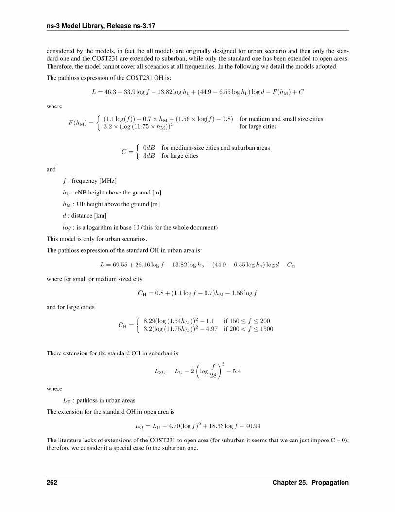
ns-3 Model Library, Release ns-3.17
considered by the models, in fact the all models are originally designed for urban scenario and then only the stan-dard one and the COST231 are extended to suburban, while only the standard one has been extended to open areas.Therefore, the model cannot cover all scenarios at all frequencies. In the following we detail the models adopted.
The pathloss expression of the COST231 OH is:
L = 46.3 + 33.9 log f − 13.82 log hb + (44.9− 6.55 log hb) log d− F (hM) + C
where
F (hM) ={
(1.1 log(f))− 0.7× hM − (1.56× log(f)− 0.8) for medium and small size cities3.2× (log (11.75× hM))2 for large cities
C ={
0dB for medium-size cities and suburban areas3dB for large cities
and
f : frequency [MHz]
hb : eNB height above the ground [m]
hM : UE height above the ground [m]
d : distance [km]
log : is a logarithm in base 10 (this for the whole document)
This model is only for urban scenarios.
The pathloss expression of the standard OH in urban area is:
L = 69.55 + 26.16 log f − 13.82 log hb + (44.9− 6.55 log hb) log d− CH
where for small or medium sized city
CH = 0.8 + (1.1 log f − 0.7)hM − 1.56 log f
and for large cities
CH ={
8.29(log (1.54hM ))2 − 1.1 if 150 ≤ f ≤ 2003.2(log (11.75hM ))2 − 4.97 if 200 < f ≤ 1500
There extension for the standard OH in suburban is
LSU = LU − 2(
logf
28
)2
− 5.4
where
LU : pathloss in urban areas
The extension for the standard OH in open area is
LO = LU − 4.70(log f)2 + 18.33 log f − 40.94
The literature lacks of extensions of the COST231 to open area (for suburban it seems that we can just impose C = 0);therefore we consider it a special case fo the suburban one.
262 Chapter 25. Propagation
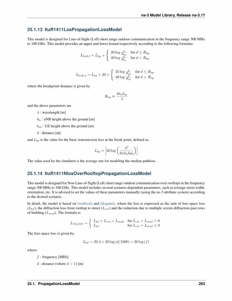
ns-3 Model Library, Release ns-3.17
25.1.13 ItuR1411LosPropagationLossModel
This model is designed for Line-of-Sight (LoS) short range outdoor communication in the frequency range 300 MHzto 100 GHz. This model provides an upper and lower bound respectively according to the following formulas
LLoS,l = Lbp +
{20 log d
Rbpfor d ≤ Rbp
40 log dRbp
for d > Rbp
LLoS,u = Lbp + 20 +
{25 log d
Rbpfor d ≤ Rbp
40 log dRbp
for d > Rbp
where the breakpoint distance is given by
Rbp ≈4hbhm
λ
and the above parameters are
λ : wavelength [m]
hb : eNB height above the ground [m]
hm : UE height above the ground [m]
d : distance [m]
and Lbp is the value for the basic transmission loss at the break point, defined as:
Lbp =∣∣∣∣20 log
(λ2
8πhbhm
)∣∣∣∣The value used by the simulator is the average one for modeling the median pathloss.
25.1.14 ItuR1411NlosOverRooftopPropagationLossModel
This model is designed for Non-Line-of-Sight (LoS) short range outdoor communication over rooftops in the frequencyrange 300 MHz to 100 GHz. This model includes several scenario-dependent parameters, such as average street width,orientation, etc. It is advised to set the values of these parameters manually (using the ns-3 attribute system) accordingto the desired scenario.
In detail, the model is based on [walfisch] and [ikegami], where the loss is expressed as the sum of free-space loss(Lbf ), the diffraction loss from rooftop to street (Lrts) and the reduction due to multiple screen diffraction past rowsof building (Lmsd). The formula is:
LNLOS1 ={Lbf + Lrts + Lmsd for Lrts + Lmsd > 0Lbf for Lrts + Lmsd ≤ 0
The free-space loss is given by:
Lbf = 32.4 + 20 log (d/1000) + 20 log (f)
where:
f : frequency [MHz]
d : distance (where d > 1) [m]
25.1. PropagationLossModel 263
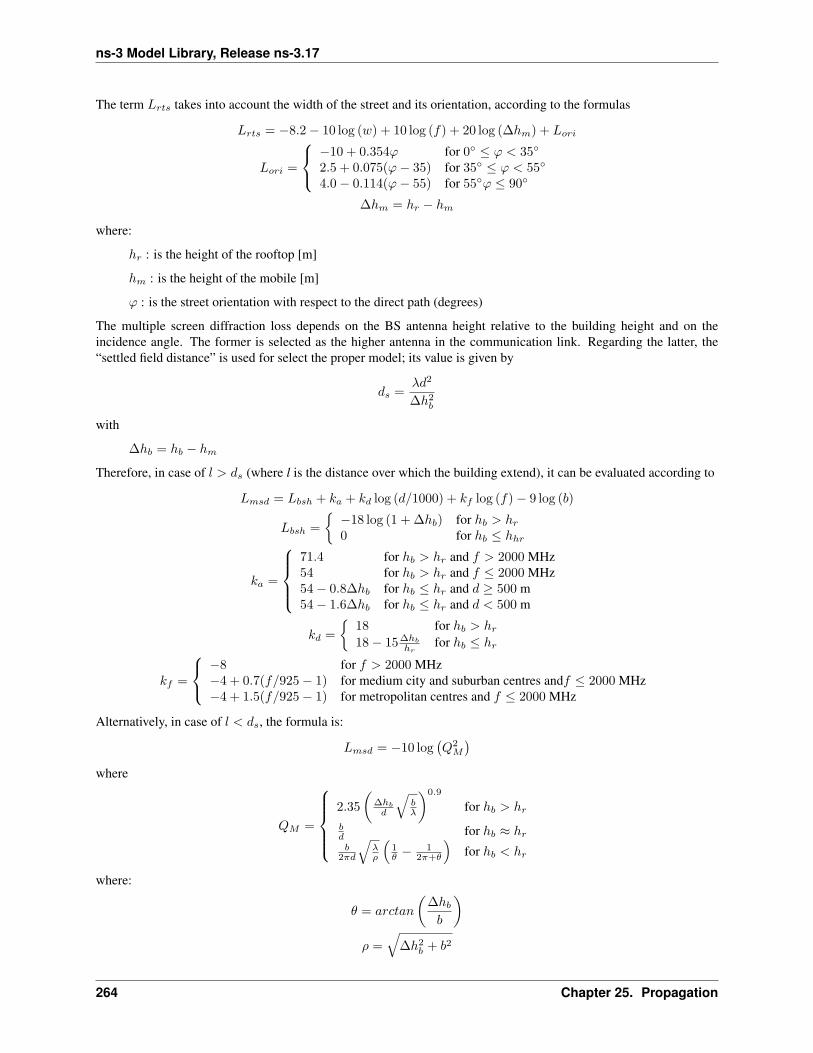
ns-3 Model Library, Release ns-3.17
The term Lrts takes into account the width of the street and its orientation, according to the formulas
Lrts = −8.2− 10 log (w) + 10 log (f) + 20 log (∆hm) + Lori
Lori =
−10 + 0.354ϕ for 0◦ ≤ ϕ < 35◦
2.5 + 0.075(ϕ− 35) for 35◦ ≤ ϕ < 55◦
4.0− 0.114(ϕ− 55) for 55◦ϕ ≤ 90◦
∆hm = hr − hm
where:
hr : is the height of the rooftop [m]
hm : is the height of the mobile [m]
ϕ : is the street orientation with respect to the direct path (degrees)
The multiple screen diffraction loss depends on the BS antenna height relative to the building height and on theincidence angle. The former is selected as the higher antenna in the communication link. Regarding the latter, the“settled field distance” is used for select the proper model; its value is given by
ds =λd2
∆h2b
with
∆hb = hb − hmTherefore, in case of l > ds (where l is the distance over which the building extend), it can be evaluated according to
Lmsd = Lbsh + ka + kd log (d/1000) + kf log (f)− 9 log (b)
Lbsh ={−18 log (1 + ∆hb) for hb > hr0 for hb ≤ hhr
ka =
71.4 for hb > hr and f > 2000 MHz54 for hb > hr and f ≤ 2000 MHz54− 0.8∆hb for hb ≤ hr and d ≥ 500 m54− 1.6∆hb for hb ≤ hr and d < 500 m
kd ={
18 for hb > hr18− 15∆hb
hrfor hb ≤ hr
kf =
−8 for f > 2000 MHz−4 + 0.7(f/925− 1) for medium city and suburban centres andf ≤ 2000 MHz−4 + 1.5(f/925− 1) for metropolitan centres and f ≤ 2000 MHz
Alternatively, in case of l < ds, the formula is:
Lmsd = −10 log(Q2M
)where
QM =
2.35
(∆hb
d
√bλ
)0.9
for hb > hr
bd for hb ≈ hrb
2πd
√λρ
(1θ −
12π+θ
)for hb < hr
where:
θ = arctan
(∆hbb
)ρ =
√∆h2
b + b2
264 Chapter 25. Propagation

ns-3 Model Library, Release ns-3.17
25.1.15 Kun2600MhzPropagationLossModel
This is the empirical model for the pathloss at 2600 MHz for urban areas which is described in [kun2600mhz]. Themodel is as follows. Let d be the distance between the transmitter and the receiver in meters; the pathloss L in dB iscalculated as:
L = 36 + 26 log d
25.2 PropagationDelayModel
The following propagation delay models are implemented:
25.2.1 PropagationDelayModel
25.2.2 RandomPropagationDelayModel
25.2.3 ConstantSpeedPropagationDelayModel
25.2. PropagationDelayModel 265

ns-3 Model Library, Release ns-3.17
266 Chapter 25. Propagation
CHAPTER
TWENTYSIX
STATISTICAL FRAMEWORK
This chapter outlines work on simulation data collection and the statistical framework for ns-3.
The source code for the statistical framework lives in the directory src/stats.
26.1 Goals
Primary objectives for this effort are the following:
• Provide functionality to record, calculate, and present data and statistics for analysis of network simulations.
• Boost simulation performance by reducing the need to generate extensive trace logs in order to collect data.
• Enable simulation control via online statistics, e.g. terminating simulations or repeating trials.
Derived sub-goals and other target features include the following:
• Integration with the existing ns-3 tracing system as the basic instrumentation framework of the internal simula-tion engine, e.g. network stacks, net devices, and channels.
• Enabling users to utilize the statistics framework without requiring use of the tracing system.
• Helping users create, aggregate, and analyze data over multiple trials.
• Support for user created instrumentation, e.g. of application specific events and measures.
• Low memory and CPU overhead when the package is not in use.
• Leveraging existing analysis and output tools as much as possible. The framework may provide some basicstatistics, but the focus is on collecting data and making it accessible for manipulation in established tools.
• Eventual support for distributing independent replications is important but not included in the first round offeatures.
26.2 Overview
The statistics framework includes the following features:
• The core framework and two basic data collectors: A counter, and a min/max/avg/total observer.
• Extensions of those to easily work with times and packets.
• Plaintext output formatted for omnetpp.
• Database output using sqlite3, a standalone, lightweight, high performance SQL engine.
267
ns-3 Model Library, Release ns-3.17
• Mandatory and open ended metadata for describing and working with runs.
• An example based on the notional experiment of examining the properties of NS-3’s default ad hoc WiFi per-formance. It incorporates the following:
– Constructs of a two node ad hoc WiFi network, with the nodes a parameterized distance apart.
– UDP traffic source and sink applications with slightly different behavior and measurement hooks than thestock classes.
– Data collection from the NS-3 core via existing trace signals, in particular data on frames transmitted andreceived by the WiFi MAC objects.
– Instrumentation of custom applications by connecting new trace signals to the stat framework, as well asvia direct updates. Information is recorded about total packets sent and received, bytes transmitted, andend-to-end delay.
– An example of using packet tags to track end-to-end delay.
– A simple control script which runs a number of trials of the experiment at varying distances and queriesthe resulting database to produce a graph using GNUPlot.
26.3 To-Do
High priority items include:
• Inclusion of online statistics code, e.g. for memory efficient confidence intervals.
• Provisions in the data collectors for terminating runs, i.e. when a threshold or confidence is met.
• Data collectors for logging samples over time, and output to the various formats.
• Demonstrate writing simple cyclic event glue to regularly poll some value.
Each of those should prove straightforward to incorporate in the current framework.
26.4 Approach
The framework is based around the following core principles:
• One experiment trial is conducted by one instance of a simulation program, whether in parallel or serially.
• A control script executes instances of the simulation, varying parameters as necessary.
• Data is collected and stored for plotting and analysis using external scripts and existing tools.
• Measures within the ns-3 core are taken by connecting the stat framework to existing trace signals.
• Trace signals or direct manipulation of the framework may be used to instrument custom simulation code.
Those basic components of the framework and their interactions are depicted in the following figure.
268 Chapter 26. Statistical Framework
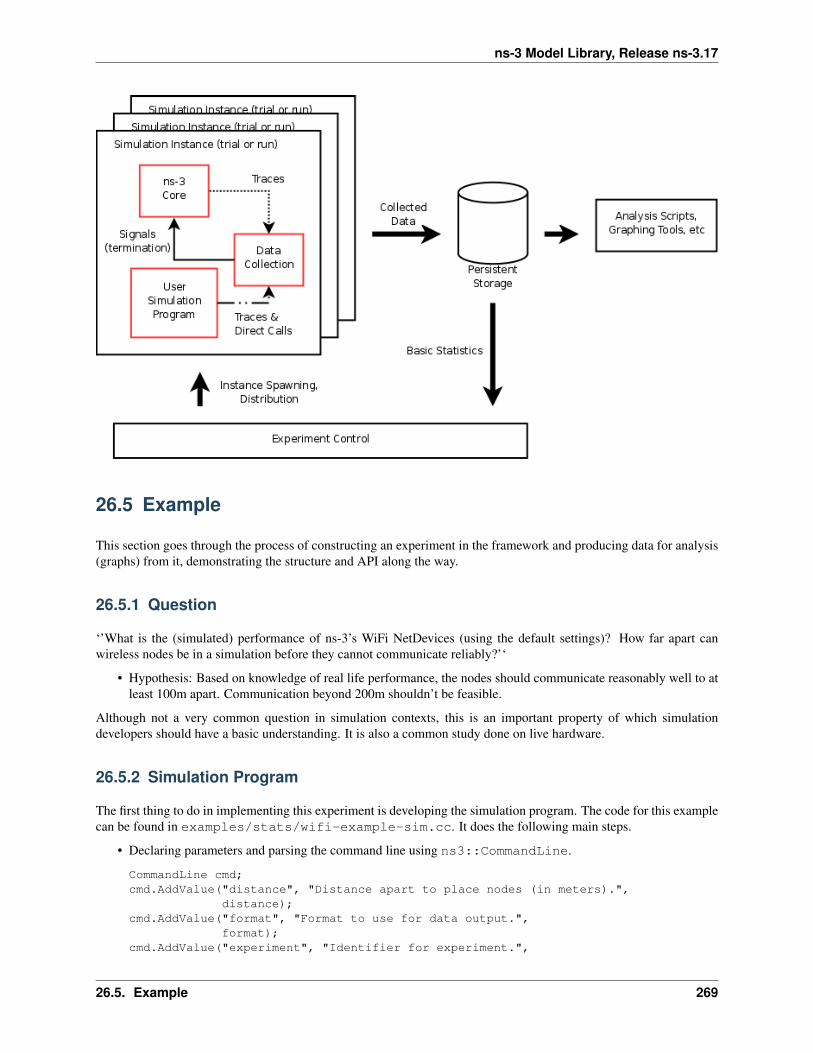
ns-3 Model Library, Release ns-3.17
26.5 Example
This section goes through the process of constructing an experiment in the framework and producing data for analysis(graphs) from it, demonstrating the structure and API along the way.
26.5.1 Question
‘’What is the (simulated) performance of ns-3’s WiFi NetDevices (using the default settings)? How far apart canwireless nodes be in a simulation before they cannot communicate reliably?’‘
• Hypothesis: Based on knowledge of real life performance, the nodes should communicate reasonably well to atleast 100m apart. Communication beyond 200m shouldn’t be feasible.
Although not a very common question in simulation contexts, this is an important property of which simulationdevelopers should have a basic understanding. It is also a common study done on live hardware.
26.5.2 Simulation Program
The first thing to do in implementing this experiment is developing the simulation program. The code for this examplecan be found in examples/stats/wifi-example-sim.cc. It does the following main steps.
• Declaring parameters and parsing the command line using ns3::CommandLine.
CommandLine cmd;cmd.AddValue("distance", "Distance apart to place nodes (in meters).",
distance);cmd.AddValue("format", "Format to use for data output.",
format);cmd.AddValue("experiment", "Identifier for experiment.",
26.5. Example 269
ns-3 Model Library, Release ns-3.17
experiment);cmd.AddValue("strategy", "Identifier for strategy.",
strategy);cmd.AddValue("run", "Identifier for run.",
runID);cmd.Parse (argc, argv);
• Creating nodes and network stacks using ns3::NodeContainer, ns3::WiFiHelper, andns3::InternetStackHelper.
NodeContainer nodes;nodes.Create(2);
WifiHelper wifi;wifi.SetMac("ns3::AdhocWifiMac");wifi.SetPhy("ns3::WifiPhy");NetDeviceContainer nodeDevices = wifi.Install(nodes);
InternetStackHelper internet;internet.Install(nodes);Ipv4AddressHelper ipAddrs;ipAddrs.SetBase("192.168.0.0", "255.255.255.0");ipAddrs.Assign(nodeDevices);
• Positioning the nodes using ns3::MobilityHelper. By default the nodes have static mobility and won’tmove, but must be positioned the given distance apart. There are several ways to do this; it is done here usingns3::ListPositionAllocator, which draws positions from a given list.
MobilityHelper mobility;Ptr<ListPositionAllocator> positionAlloc =CreateObject<ListPositionAllocator>();
positionAlloc->Add(Vector(0.0, 0.0, 0.0));positionAlloc->Add(Vector(0.0, distance, 0.0));mobility.SetPositionAllocator(positionAlloc);mobility.Install(nodes);
• Installing a traffic generator and a traffic sink. The stock Applications could be used, but the exampleincludes custom objects in src/test/test02-apps.(cc|h). These have a simple behavior, generatinga given number of packets spaced at a given interval. As there is only one of each they are installed manually;for a larger set the ns3::ApplicationHelper class could be used. The commented-out Config::Setline changes the destination of the packets, set to broadcast by default in this example. Note that in generalWiFi may have different performance for broadcast and unicast frames due to different rate control and MACretransmission policies.
Ptr<Node> appSource = NodeList::GetNode(0);Ptr<Sender> sender = CreateObject<Sender>();appSource->AddApplication(sender);sender->Start(Seconds(1));
Ptr<Node> appSink = NodeList::GetNode(1);Ptr<Receiver> receiver = CreateObject<Receiver>();appSink->AddApplication(receiver);receiver->Start(Seconds(0));
// Config::Set("/NodeList/*/ApplicationList/*/$Sender/Destination",// Ipv4AddressValue("192.168.0.2"));
• Configuring the data and statistics to be collected. The basic paradigm is that an ns3::DataCollectorobject is created to hold information about this particular run, to which observers and calculators are attached to
270 Chapter 26. Statistical Framework
ns-3 Model Library, Release ns-3.17
actually generate data. Importantly, run information includes labels for the ‘’experiment’‘, ‘’strategy’‘, ‘’input’‘,and ‘’run’‘. These are used to later identify and easily group data from multiple trials.
– The experiment is the study of which this trial is a member. Here it is on WiFi performance and distance.
– The strategy is the code or parameters being examined in this trial. In this example it is fixed, but anobvious extension would be to investigate different WiFi bit rates, each of which would be a differentstrategy.
– The input is the particular problem given to this trial. Here it is simply the distance between the two nodes.
– The runID is a unique identifier for this trial with which it’s information is tagged for identification in lateranalysis. If no run ID is given the example program makes a (weak) run ID using the current time.
Those four pieces of metadata are required, but more may be desired. They may be added to the record usingthe ns3::DataCollector::AddMetadata() method.
DataCollector data;data.DescribeRun(experiment,
strategy,input,runID);
data.AddMetadata("author", "tjkopena");
Actual observation and calculating is done by ns3::DataCalculator objects, of which several differenttypes exist. These are created by the simulation program, attached to reporting or sampling code, and thenregistered with the ns3::DataCollector so they will be queried later for their output. One easy observationmechanism is to use existing trace sources, for example to instrument objects in the ns-3 core without changingtheir code. Here a counter is attached directly to a trace signal in the WiFi MAC layer on the target node.
Ptr<PacketCounterCalculator> totalRx =CreateObject<PacketCounterCalculator>();
totalRx->SetKey("wifi-rx-frames");Config::Connect("/NodeList/1/DeviceList/*/$ns3::WifiNetDevice/Rx",
MakeCallback(&PacketCounterCalculator::FrameUpdate,totalRx));
data.AddDataCalculator(totalRx);
Calculators may also be manipulated directly. In this example, a counter is created and passed to the traffic sinkapplication to be updated when packets are received.
Ptr<CounterCalculator<> > appRx =CreateObject<CounterCalculator<> >();
appRx->SetKey("receiver-rx-packets");receiver->SetCounter(appRx);data.AddDataCalculator(appRx);
To increment the count, the sink’s packet processing code then calls one of the calculator’s update methods.
m_calc->Update();
The program includes several other examples as well, using both the primitive calculators suchas ns3::CounterCalculator and those adapted for observing packets and times. Insrc/test/test02-apps.(cc|h) it also creates a simple custom tag which it uses to track end-to-end delay for generated packets, reporting results to a ns3::TimeMinMaxAvgTotalCalculator datacalculator.
• Running the simulation, which is very straightforward once constructed.
Simulator::Run();
26.5. Example 271

ns-3 Model Library, Release ns-3.17
• Generating either omnetpp or sqlite output, depending on the command line arguments. To do this ans3::DataOutputInterface object is created and configured. The specific type of this will determine theoutput format. This object is then given the ns3::DataCollector object which it interrogates to producethe output.
Ptr<DataOutputInterface> output;if (format == "omnet") {NS_LOG_INFO("Creating omnet formatted data output.");output = CreateObject<OmnetDataOutput>();
} else {#ifdef STAT_USE_DB
NS_LOG_INFO("Creating sqlite formatted data output.");output = CreateObject<SqliteDataOutput>();
#endif}
output->Output(data);
• Freeing any memory used by the simulation. This should come at the end of the main function for the example.
Simulator::Destroy();
Logging
To see what the example program, applications, and stat framework are doing in detail, set the NS_LOG variableappropriately. The following will provide copious output from all three.
export NS_LOG=StatFramework:WiFiDistanceExperiment:WiFiDistanceApps
Note that this slows down the simulation extraordinarily.
Sample Output
Compiling and simply running the test program will append omnet++ formatted output such as the following todata.sca.
run run-1212239121
attr experiment "wifi-distance-test"attr strategy "wifi-default"attr input "50"attr description ""
attr "author" "tjkopena"
scalar wifi-tx-frames count 30scalar wifi-rx-frames count 30scalar sender-tx-packets count 30scalar receiver-rx-packets count 30scalar tx-pkt-size count 30scalar tx-pkt-size total 1920scalar tx-pkt-size average 64scalar tx-pkt-size max 64scalar tx-pkt-size min 64scalar delay count 30scalar delay total 5884980nsscalar delay average 196166ns
272 Chapter 26. Statistical Framework
ns-3 Model Library, Release ns-3.17
scalar delay max 196166nsscalar delay min 196166ns
26.5.3 Control Script
In order to automate data collection at a variety of inputs (distances), a simple Bash script is used to execute a seriesof simulations. It can be found at examples/stats/wifi-example-db.sh. The script runs through a set ofdistances, collecting the results into an sqlite3 database. At each distance five trials are conducted to give a betterpicture of expected performance. The entire experiment takes only a few dozen seconds to run on a low end machineas there is no output during the simulation and little traffic is generated.
#!/bin/sh
DISTANCES="25 50 75 100 125 145 147 150 152 155 157 160 162 165 167 170 172 175 177 180"TRIALS="1 2 3 4 5"
echo WiFi Experiment Example
if [ -e data.db ]then
echo Kill data.db?read ANSif [ "$ANS" = "yes" -o "$ANS" = "y" ]thenecho Deleting databaserm data.db
fifi
for trial in $TRIALSdo
for distance in $DISTANCESdoecho Trial $trial, distance $distance./bin/test02 --format=db --distance=$distance --run=run-$distance-$trial
donedone
26.5.4 Analysis and Conclusion
Once all trials have been conducted, the script executes a simple SQL query over the database using the sqlite3command line program. The query computes average packet loss in each set of trials associated with each distance.It does not take into account different strategies, but the information is present in the database to make some simpleextensions and do so. The collected data is then passed to GNUPlot for graphing.
CMD="select exp.input,avg(100-((rx.value*100)/tx.value)) \from Singletons rx, Singletons tx, Experiments exp \where rx.run = tx.run AND \
rx.run = exp.run AND \rx.name=’receiver-rx-packets’ AND \tx.name=’sender-tx-packets’ \
group by exp.input \order by abs(exp.input) ASC;"
sqlite3 -noheader data.db "$CMD" > wifi-default.data
26.5. Example 273
ns-3 Model Library, Release ns-3.17
sed -i "s/|/ /" wifi-default.datagnuplot wifi-example.gnuplot
The GNUPlot script found at examples/stats/wifi-example.gnuplot simply defines the output formatand some basic formatting for the graph.
set terminal postscript portrait enhanced lw 2 "Helvetica" 14
set size 1.0, 0.66
#-------------------------------------------------------set out "wifi-default.eps"#set title "Packet Loss Over Distance"set xlabel "Distance (m) --- average of 5 trials per point"set xrange [0:200]set ylabel "% Packet Loss"set yrange [0:110]
plot "wifi-default.data" with lines title "WiFi Defaults"
End Result
The resulting graph provides no evidence that the default WiFi model’s performance is necessarily unreasonable andlends some confidence to an at least token faithfulness to reality. More importantly, this simple investigation has beencarried all the way through using the statistical framework. Success!
274 Chapter 26. Statistical Framework
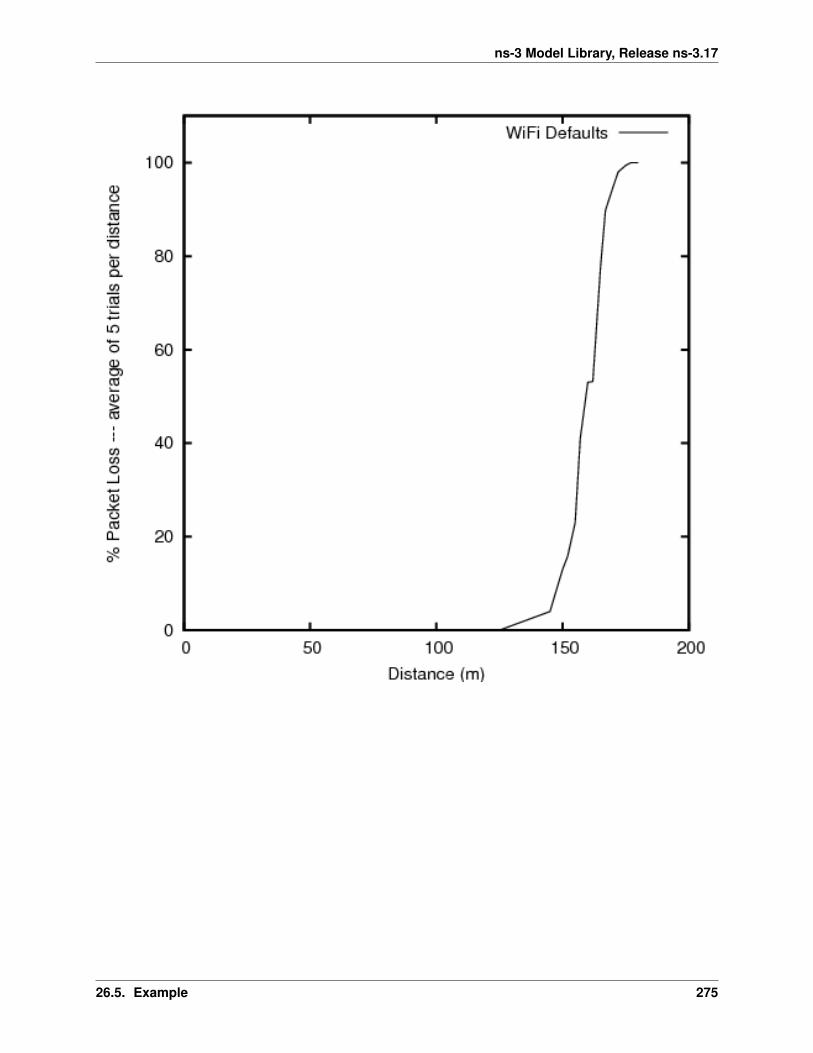
ns-3 Model Library, Release ns-3.17
26.5. Example 275

ns-3 Model Library, Release ns-3.17
276 Chapter 26. Statistical Framework
CHAPTER
TWENTYSEVEN
TOPOLOGY INPUT READERS
The topology modules aim at reading a topology file generated by an automatic topology generator.
The process is divided in two steps:
• running a topology generator to build a topology file
• reading the topology file and build a ns-3 simulation
Hence, model is focused on being able to read correctly the various topology formats.
Currently there are three models:
• ns3::OrbisTopologyReader for Orbis 0.7 traces
• ns3::InetTopologyReader for Inet 3.0 traces
• ns3::RocketfuelTopologyReader for Rocketfuel traces
An helper ns3::TopologyReaderHelper is provided to assist on trivial tasks.
A good source for topology data is also Archipelago.
The current Archipelago Measurements, monthly updated, are stored in the CAIDA website using a complete notationand triple data source, one for each working group.
A different and more compact notation reporting only the AS-relationships (a sort of more Orbis-like format) is here:as-relationships.
The compact notation can be easily stripped down to a pure Orbis format, just removing the double relationships (thecompact format use one-way links, while Orbis use two-way links) and pruning the 3rd parameter. Note that with thecompact data Orbis can then be used create a rescaled version of the topology, thus being the most effective way (tomy best knowledge) to make an internet-like topology.
Examples can be found in the directory src/topology-read/examples/
277

ns-3 Model Library, Release ns-3.17
278 Chapter 27. Topology Input Readers
CHAPTER
TWENTYEIGHT
UAN FRAMEWORK
The main goal of the UAN Framework is to enable researchers to model a variety of underwater network scenarios.The UAN model is broken into four main parts: The channel, PHY, MAC and Autonomous Underwater Vehicle (AUV)models.
The need for underwater wireless communications exists in applications such as remote control in offshore oil industry1, pollution monitoring in environmental systems, speech transmission between divers, mapping of the ocean floor,mine counter measures 2, seismic monitoring of ocean faults as well as climate changes monitoring. Unfortunately,making on-field measurements is very expensive and there are no commonly accepted standard to base on. Hence, thepriority to make research work going on, it is to realize a complete simulation framework that researchers can use toexperiment, make tests and make performance evaluation and comparison.
The NS-3 UAN module is a first step in this direction, trying to offer a reliable and realistic tool. In fact, the UANmodule offers accurate modelling of the underwater acoustic channel, a model of the WHOI acoustic modem (one ofthe widely used acoustic modems)[6]_ and its communications performance, and some MAC protocols.
28.1 Model Description
The source code for the UAN Framework lives in the directory src/uan and in src/energy for the contributionon the li-ion battery model.
The UAN Framework is composed of two main parts:
• the AUV mobility models, including Electric motor propelled AUV (REMUS class 3 4 ) and Seaglider 4 models
• the energy models, including AUV energy models, AUV energy sources (batteries) and an acoustic modemenergy model
As enabling component for the energy models, a Li-Ion batteries energy source has been implemented basing on 5 6.
1 BINGHAM, D.; DRAKE, T.; HILL, A.; LOTT, R.; The Application of Autonomous Underwater Vehicle (AUV) Technology in the Oil Industry– Vision and Experiences, URL: http://www.fig.net/pub/fig_2002/Ts4-4/TS4_4_bingham_etal.pdf
2 WHOI, Autonomous Underwater Vehicle, REMUS; URL: http://www.whoi.edu/page.do?pid=298563 Hydroinc Products; URL: http://www.hydroidinc.com/products.html4 Eriksen, C.C., T.J. Osse, R.D. Light, T. Wen, T.W. Lehman, P.L. Sabin, J.W. Ballard, and A.M. Chiodi. Seaglider: A Long-
Range Autonomous Underwater Vehicle for Oceanographic Research, IEEE Journal of Oceanic Engineering, 26, 4, October 2001. URL:http://ieeexplore.ieee.org/stamp/stamp.jsp?tp=&arnumber=972073&userType=inst
5 C. M. Shepherd, “Design of Primary and Secondary Cells - Part 3. Battery discharge equation,” U.S. Naval Research Laboratory, 19636 Tremblay, O.; Dessaint, L.-A.; Dekkiche, A.-I., “A Generic Battery Model for the Dynamic Simulation of Hybrid Electric Vehicles,” Ecole de
Technologie Superieure, Universite du Quebec, 2007 URL: http://ieeexplore.ieee.org/stamp/stamp.jsp?tp=&arnumber=4544139
279
ns-3 Model Library, Release ns-3.17
28.1.1 Design
UAN Propagation Models
Modelling of the underwater acoustic channel has been an active area of research for quite some time. Given thecomplications involved, surface and bottom interactions, varying speed of sound, etc..., the detailed models in use forocean acoustics research are much too complex (in terms of runtime) for use in network level simulations. We haveattempted to provide the often used models as well as make an attempt to bridge, in part, the gap between complicatedocean acoustic models and network level simulation. The three propagation models included are the ideal channelmodel, the Thorp propagation model and the Bellhop propagation model (Available as an addition).
All of the Propagation Models follow the same simple interface in ns3::UanPropModel. The propagation modelsprovide a power delay profile (PDP) and pathloss information. The PDP is retrieved using the GetPdp method whichreturns type UanPdp. ns3::UanPdp utilises a tapped delay line model for the acoustic channel. The UanPdp classis a container class for Taps, each tap has a delay and amplitude member corresponding to the time of arrival (relativeto the first tap arrival time) and amplitude. The propagation model also provides pathloss between the source andreceiver in dB re 1uPa. The PDP and pathloss can then be used to find the received signal power over a durationof time (i.e. received signal power in a symbol duration and ISI which interferes with neighbouring signals). BothUanPropModelIdeal and UanPropModelThorp return a single impulse for a PDP.
1. Ideal Channel Model ns3::UanPropModelIdeal
The ideal channel model assumes 0 pathloss inside a cylindrical area with bounds set by attribute. The ideal channelmodel also assumes an impulse PDP.
2. Thorp Propagation Model ns3::UanPropModelThorp
The Thorp Propagation Model calculates pathloss using the well-known Thorp approximation. This model is similarto the underwater channel model implemented in ns2 as described here:
Harris, A. F. and Zorzi, M. 2007. Modeling the underwater acoustic channel in ns2. In Proceedings of the 2ndinternational Conference on Performance Evaluation Methodologies and Tools (Nantes, France, October 22 - 27,2007). ValueTools, vol. 321. ICST (Institute for Computer Sciences Social-Informatics and TelecommunicationsEngineering), ICST, Brussels, Belgium, 1-8.
The frequency used in calculation however, is the center frequency of the modulation as found from ns3::UanTxMode.The Thorp Propagation Model also assumes an impulse channel response.
3. Bellhop Propagation Model ns3::UanPropModelBh (Available as an addition)
The Bellhop propagation model reads propagation information from a database. A configuration file describing thelocation, and resolution of the archived information must be supplied via attributes. We have included a utility, create-dat, which can create these data files using the Bellhop Acoustic Ray Tracing software (http://oalib.hlsresearch.com/).
The create-dat utility requires a Bellhop installation to run. Bellhop takes environment information about the channel,such as sound speed profile, surface height bottom type, water depth, and uses a gaussian ray tracing algorithm todetermine propagation information. Arrivals from Bellhop are grouped together into equal length taps (the arrivalsin a tap duration are coherently summed). The maximum taps are then aligned to take the same position in the PDP.The create-dat utility averages together several runs and then normalizes the average such that the sum of all taps is 1.The same configuration file used to create the data files using create-dat should be passed via attribute to the BellhopPropagation Model.
The Bellhop propagation model is available as a patch. The link address will be made available here when it is postedonline. Otherwise email [email protected] for more information.
UAN PHY Model Overview
The PHY has been designed to allow for relatively easy extension to new networking scenarios. We feel this isimportant as, to date, there has been no commonly accepted network level simulation model for underwater networks.
280 Chapter 28. UAN Framework
ns-3 Model Library, Release ns-3.17
The lack of commonly accepted network simulation tools has resulted in a wide array of simulators and models usedto report results in literature. The lack of standardization makes comparing results nearly impossible.
The main component of the PHY Model is the generic PHY class, ns3::UanPhyGen. The PHY class’s generalresponsibility is to handle packet acquisition, error determination, and forwarding of successful packets up to theMAC layer. The Generic PHY uses two models for determination of signal to noise ratio (SINR) and packet error rate(PER). The combination of the PER and SINR models determine successful reception of packets. The PHY modelconnects to the channel via a Transducer class. The Transducer class is responsible for tracking all arriving packetsand departing packets over the duration of the events. How the PHY class and the PER and SINR models respond topackets is based on the “Mode” of the transmission as described by the ns3::UanTxMode class.
When a MAC layer sends down a packet to the PHY for transmission it specifies a “mode number” to be used for thetransmission. The PHY class accepts, as an attribute, a list of supported modes. The mode number corresponds to anindex in the supported modes. The UanTxMode contains simple modulation information and a unique string id. Thegeneric PHY class will only acquire arriving packets which use a mode which is in the supported modes list of thePHY. The mode along with received signal power, and other pertinent attributes (e.g. possibly interfering packets andtheir modes) are passed to the SINR and PER models for calculation of SINR and probability of error.
Several simple example PER and SINR models have been created. a) The PER models - Default (simple) PER model(ns3::UanPhyPerGenDefault): The Default PER model tests the packet against a threshold and assumes error(with prob. 1) if the SINR is below the threshold or success if the SINR is above the threshold - Micromodem FH-FSKPER (ns3::UanPhyPerUmodem). The FH-FSK PER model calculates probability of error assuming a rate 1/2convolutional code with constraint length 9 and a CRC check capable of correcting up to 1 bit error. This is similar towhat is used in the receiver of the WHOI Micromodem.
b) SINR models - Default Model (ns3::UanPhyCalcSinrDefault), The default SINR model assumes that alltransmitted energy is captured at the receiver and that there is no ISI. Any received signal power from interferes actsas additional ambient noise. - FH-FSK SINR Model (ns3::UanPhyCalcSinrFhFsk), The WHOI Micromodemoperating in FH-FSK mode uses a predetermined hopping pattern that is shared by all nodes in the network. Wemodel this by only including signal energy receiving within one symbol time (as given by ns3::UanTxMode) incalculating the received signal power. A channel clearing time is given to the FH-FSK SINR model via attribute. Anysignal energy arriving in adjacent signals (after a symbol time and the clearing time) is considered ISI and is treatedas additional ambient noise. Interfering signal arrivals inside a symbol time (any symbol time) is also counted asadditional ambient noise - Frequency filtered SINR (ns3::UanPhyCalcSinrDual). This SINR model calculatesSINR in the same manner as the default model. This model however only considers interference if there is an overlapin frequency of the arriving packets as determined by UanTxMode.
In addition to the generic PHY a dual phy layer is also included (ns3::UanPhyDual). This wraps two generic phylayers together to model a net device which includes two receivers. This was primarily developed for UanMacRc,described in the next section.
UAN MAC Model Overview
Over the last several years there have been a myriad of underwater MAC proposals in the literature. We have includedthree MAC protocols with this distribution: a) CW-MAC, a MAC protocol which uses a slotted contention windowsimilar in nature to the IEEE 802.11 DCF. Nodes have a constant contention window measured in slot times (configuredvia attribute). If the channel is sensed busy, then nodes backoff by randomly (uniform distribution) choose a slot totransmit in. The slot time durations are also configured via attribute. This MAC was described in
Parrish N.; Tracy L.; Roy S. Arabshahi P.; and Fox, W., System Design Considerations for Undersea Networks:Link and Multiple Access Protocols , IEEE Journal on Selected Areas in Communications (JSAC), Special Issue onUnderwater Wireless Communications and Networks, Dec. 2008.
b) RC-MAC (ns3::UanMacRc ns3::UanMacRcGw) a reservation channel protocol which dynamically dividesthe available bandwidth into a data channel and a control channel. This MAC protocol assumes there is a gateway nodewhich all network traffic is destined for. The current implementation assumes a single gateway and a single networkneighborhood (a single hop network). RTS/CTS handshaking is used and time is divided into cycles. Non-gateway
28.1. Model Description 281
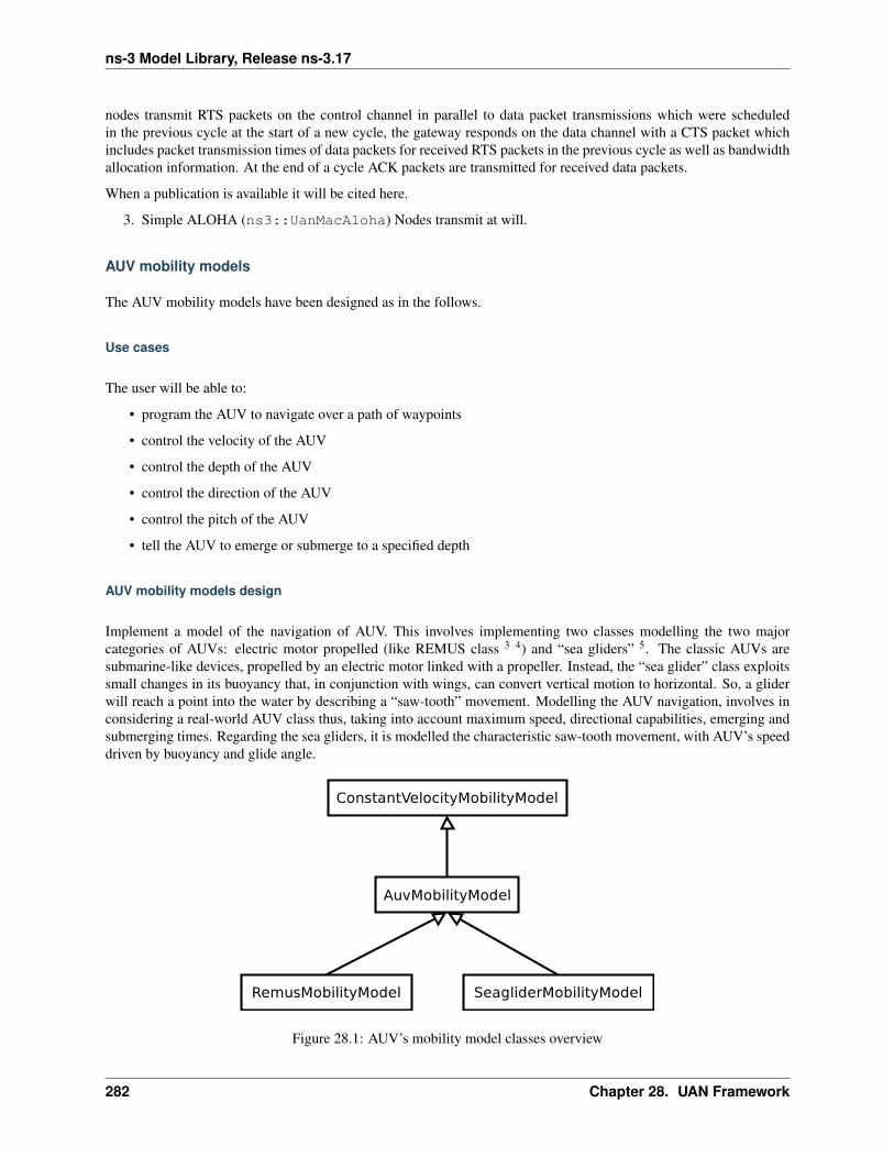
ns-3 Model Library, Release ns-3.17
nodes transmit RTS packets on the control channel in parallel to data packet transmissions which were scheduledin the previous cycle at the start of a new cycle, the gateway responds on the data channel with a CTS packet whichincludes packet transmission times of data packets for received RTS packets in the previous cycle as well as bandwidthallocation information. At the end of a cycle ACK packets are transmitted for received data packets.
When a publication is available it will be cited here.
3. Simple ALOHA (ns3::UanMacAloha) Nodes transmit at will.
AUV mobility models
The AUV mobility models have been designed as in the follows.
Use cases
The user will be able to:
• program the AUV to navigate over a path of waypoints
• control the velocity of the AUV
• control the depth of the AUV
• control the direction of the AUV
• control the pitch of the AUV
• tell the AUV to emerge or submerge to a specified depth
AUV mobility models design
Implement a model of the navigation of AUV. This involves implementing two classes modelling the two majorcategories of AUVs: electric motor propelled (like REMUS class 3 4) and “sea gliders” 5. The classic AUVs aresubmarine-like devices, propelled by an electric motor linked with a propeller. Instead, the “sea glider” class exploitssmall changes in its buoyancy that, in conjunction with wings, can convert vertical motion to horizontal. So, a gliderwill reach a point into the water by describing a “saw-tooth” movement. Modelling the AUV navigation, involves inconsidering a real-world AUV class thus, taking into account maximum speed, directional capabilities, emerging andsubmerging times. Regarding the sea gliders, it is modelled the characteristic saw-tooth movement, with AUV’s speeddriven by buoyancy and glide angle.
Figure 28.1: AUV’s mobility model classes overview
282 Chapter 28. UAN Framework
ns-3 Model Library, Release ns-3.17
An ns3::AuvMobilityModel interface has been designed to give users a generic interface to access AUV’s nav-igation functions. The AuvMobilityModel interface is implemented by the RemusMobilityModel and the GliderMo-bilityModel classes. The AUV’s mobility models organization it is shown in AUV’s mobility model classes overview.Both models use a constant velocity movement, thus the AuvMobilityModel interface derives from the ConstantVe-locityMobilityModel. The two classes hold the navigation parameters for the two different AUVs, like maximum pitchangles, maximum operating depth, maximum and minimum speed values. The Glider model holds also some extraparameters like maximum buoyancy values, and maximum and minimum glide slopes. Both classes, RemusMobility-Model and GliderMobilityModel, handle also the AUV power consumption, utilizing the relative power models. Hasbeen modified the WaypointMobilityModel to let it use a generic underlying ConstantVelocityModel to validate thewaypoints and, to keep trace of the node’s position. The default model is the classic ConstantVelocityModel but, forexample in case of REMUS mobility model, the user can install the AUV mobility model into the waypoint model andthen validating the waypoints against REMUS navigation constraints.
Energy models
The energy models have been designed as in the follows.
Use cases
The user will be able to:
• use a specific power profile for the acoustic modem
• use a specific energy model for the AUV
• trace the power consumption of AUV navigation, through AUV’s energy model
• trace the power consumprion underwater acoustic communications, through acoustic modem power profile
We have integrated the Energy Model with the UAN module, to implement energy handling. We have implemented aspecific energy model for the two AUV classes and, an energy source for Lithium batteries. This will be really usefulfor researchers to keep trace of the AUV operational life. We have implemented also an acoustic modem power profile,to keep trace of its power consumption. This can be used to compare protocols specific power performance. In orderto use such power profile, the acoustic transducer physical layer has been modified to use the modem power profile.We have decoupled the physical layer from the transducer specific energy model, to let the users change the differentenergy models without changing the physical layer.
AUV energy models
Basing on the Device Energy Model interface, it has been implemented a specific energy model for the two AUVclasses (REMUS and Seaglider). This models reproduce the AUV’s specific power consumption to give users accurateinformation. This model can be naturally used to evaluates the AUV operating life, as well as mission-related powerconsumption, etc. Have been developed two AUV energy models:
• GliderEnergyModel, computes the power consumption of the vehicle based on the current buoyancy value andvertical speed 5
• RemusEnergyModel, computes the power consumption of the vehicle based on the current speed, as it is pro-pelled by a brush-less electric motor
Note: TODO extend a little bit
28.1. Model Description 283

ns-3 Model Library, Release ns-3.17
AUV energy sources
Note: [TODO]
Acoustic modem energy model
Basing on the Device Energy Model interface, has been implemented a generic energy model for acoustic modem. Themodel allows to trace four modem’s power-states: Sleep, Idle, Receiving, Transmitting. The default parameters forthe energy model are set to fit those of the WHOI µmodem. The class follows pretty closely the RadioEnergyModelclass as the transducer behaviour is pretty close to that of a wifi radio.
The default power consumption values implemented into the model are as follows [6]:
Modem State Power ConsumptionTX 50 WRX 158 mWIdle 158 mWSleep 5.8 mW
UAN module energy modifications
The UAN module has been modified in order to utilize the implemented energy classes. Specifically, it has beenmodified the physical layer of the UAN module. It Has been implemented an UpdatePowerConsumption method thattakes the modem’s state as parameter. It checks if an energy source is installed into the node and, in case, it thenuse the AcousticModemEnergyModel to update the power consumption with the current modem’s state. The modempower consumption’s update takes place whenever the modem changes its state.
A user should take into account that, if the the power consumption handling is enabled (if the node has an energysource installed), all the communications processes will terminate whether the node depletes all the energy source.
Li-Ion batteries model
A generic Li-Ion battery model has been implemented based on [7][8]. The model can be fitted to any type of Li-Ionbattery simply changing the model’s parameters The default values are fitted for the Panasonic CGR18650DA Li-IonBattery [9]. [TODO insert figure] As shown in figure the model approximates very well the Li-Ion cells. RegardingSeagliders, the batteries used into the AUV are Electrochem 3B36 Lithium / Sulfuryl Chloride cells [10]. Also withthis cell type, the model seems to approximates the different discharge curves pretty well, as shown in the figure.
Note: should I insert the li-ion model deatils here? I think it is better to put them into an Energy-related chapter..
28.1.2 Scope and Limitations
The framework is designed to simulate AUV’s behaviour. We have modeled the navigation and power consumptionbehaviour of REMUS class and Seaglider AUVs. The communications stack, associated with the AUV, can be modi-fied depending on simulation needs. Usually, the default underwater stack is being used, composed of an half duplexacoustic modem, an Aloha MAC protocol and a generic physical layer.
Regarding the AUV energy consumption, the user should be aware that the level of accuracy differs for the two classes:
284 Chapter 28. UAN Framework
ns-3 Model Library, Release ns-3.17
• Seaglider, high level of accuracy, thanks to the availability of detailed information on AUV’s components andbehaviour [5] [10]. Have been modeled both the navigation power consumption and the Li battery packs (ac-cording to [5]).
• REMUS, medium level of accuracy, due to the lack of publicly available information on AUV’s components.We have approximated the power consumption of the AUV’s motor with a linear behaviour and, the energysource uses an ideal model (BasicEnergySource) with a power capacity equal to that specified in [4].
28.1.3 Future Work
Some ideas could be :
• insert a data logging capability
• modify the framework to use sockets (enabling the possibility to use applications)
• introduce some more MAC protocols
• modify the physical layer to let it consider the doppler spread (problematic in underwater environments)
• introduce OFDM modulations
28.1.4 References
28.2 Usage
The main way that users who write simulation scripts will typically interact with the UAN Framework is through thehelper API and through the publicly visible attributes of the model.
The helper API is defined in src/uan/helper/acoustic-modem-energy-model-helper.{cc,h} andin /src/uan/helper/...{cc,h}.
The example folder src/uan/examples/ contain some basic code that shows how to set up and use the models.further examples can be found into the Unit tests in src/uan/test/...cc
28.2.1 Examples
Examples of the Framework’s usage can be found into the examples folder. There are mobility related examples anduan related ones.
Mobility Model Examples
• auv-energy-model: In this example we show the basic usage of an AUV energy model. Specifically, weshow how to create a generic node, adding to it a basic energy source and consuming energy from theenergy source. In this example we show the basic usage of an AUV energy model.
The Seaglider AUV power consumption depends on buoyancy and vertical speed values, so we simulate a20 seconds movement at 0.3 m/s of vertical speed and 138g of buoyancy. Then a 20 seconds movement at0.2 m/s of vertical speed and 138g of buoyancy and then a stop of 5 seconds.
The required energy will be drained by the model basing on the given buoyancy/speed values, from theenergy source installed onto the node. We finally register a callback to the TotalEnergyConsumption tracedvalue.
28.2. Usage 285
ns-3 Model Library, Release ns-3.17
• auv-mobility: In this example we show how to use the AuvMobilityHelper to install an AUV mobilitymodel into a (set of) node. Then we make the AUV to submerge to a depth of 1000 meters. We then seta callback function called on reaching of the target depth. The callback then makes the AUV to emergeto water surface (0 meters). We set also a callback function called on reaching of the target depth. Theemerge callback then, stops the AUV.
During the whole navigation process, the AUV’s position is tracked by the TracePos function and plottedinto a Gnuplot graph.
• waypoint-mobility: We show how to use the WaypointMobilityModel with a non-standard ConstantVe-locityMobilityModel. We first create a waypoint model with an underlying RemusMobilityModel settingthe mobility trace with two waypoints. We then create a waypoint model with an underlying GliderMobil-ityModel setting the waypoints separately with the AddWaypoint method. The AUV’s position is printedout every seconds.
UAN Examples
• li-ion-energy-source In this simple example, we show how to create and drain energy from a LiIonEn-ergySource. We make a series of discharge calls to the energy source class, with different current drain anddurations, until all the energy is depleted from the cell (i.e. the voltage of the cell goes below the thresholdlevel). Every 20 seconds we print out the actual cell voltage to verify that it follows the discharge curve[9]. At the end of the example it is verified that after the energy depletion call, the cell voltage is below thethreshold voltage.
• uan-energy-auv This is a comprehensive example where all the project’s components are used. We setuptwo nodes, one fixed surface gateway equipped with an acoustic modem and a moving Seaglider AUV withan acoustic modem too. Using the waypoint mobility model with an underlying GliderMobilityModel, wemake the glider descend to -1000 meters and then emerge to the water surface. The AUV sends a generic17-bytes packet every 10 seconds during the navigation process. The gateway receives the packets andstores the total bytes amount. At the end of the simulation are shown the energy consumptions of the twonodes and the networking stats.
28.2.2 Helpers
In this section we give an overview of the available helpers and their behaviour.
AcousticModemEnergyModelHelper
This helper installs AcousticModemEnergyModel into UanNetDevice objects only. It requires an UanNetDevice andan EnergySource as input objects.
The helper creates an AcousticModemEnergyModel with default parameters and associate it with the given energysource. It configures an EnergyModelCallback and an EnergyDepletionCallback. The depletion callback can beconfigured as a parameter.
AuvGliderHelper
Installs into a node (or set of nodes) the Seaglider’s features:
• waypoint model with underlying glider mobility model
• glider energy model
• glider energy source
286 Chapter 28. UAN Framework

ns-3 Model Library, Release ns-3.17
• micro modem energy model
The glider mobility model is the GliderMobilityModel with default parameters. The glider energy model is the Glid-erEnergyModel with default parameters.
Regarding the energy source, the Seaglider features two battery packs, one for motor power and one for digital-analogpower. Each pack is composed of 12 (10V) and 42 (24V) lithium chloride DD-cell batteries, respectively [5]. Thetotal power capacity is around 17.5 MJ (3.9 MJ + 13.6 MJ). In the original version of the Seaglider there was 18 + 63D-cell with a total power capacity of 10MJ.
The packs design is as follows:
• 10V - 3 in-series string x 4 strings = 12 cells - typical capacity ~100 Ah
• 24V - 7 in-series-strings x 6 strings = 42 cells - typical capacity ~150 Ah
Battery cells are Electrochem 3B36, with 3.6 V nominal voltage and 30.0 Ah nominal capacity. The 10V battery packis associated with the electronic devices, while the 24V one is associated with the pump motor.
The micro modem energy model is the MicroModemEnergyModel with default parameters.
AuvRemusHelper
Install into a node (or set of nodes) the REMUS features:
• waypoint model with REMUS mobility model validation
• REMUS energy model
• REMUS energy source
• micro modem energy model
The REMUS mobility model is the RemusMobilityModel with default parameters. The REMUS energy model is theRemusEnergyModel with default parameters.
Regarding the energy source, the REMUS features a rechargeable lithium ion battery pack rated 1.1 kWh @ 27 V(40 Ah) in operating conditions (specifications from [3] and Hydroinc European salesman). Since more detailedinformation about battery pack were not publicly available, the energy source used is a BasicEnergySource.
The micro modem energy model is the MicroModemEnergyModel with default parameters.
28.2.3 Attributes
Note: TODO
28.2.4 Tracing
Note: TODO
28.2.5 Logging
Note: TODO
28.2. Usage 287

ns-3 Model Library, Release ns-3.17
28.2.6 Caveats
Note: TODO
28.3 Validation
This model has been tested with three UNIT test:
• auv-energy-model
• auv-mobility
• li-ion-energy-source
28.3.1 Auv Energy Model
Includes test cases for single packet energy consumption, energy depletion, Glider and REMUS energy consumption.The unit test can be found in src/uan/test/auv-energy-model-test.cc.
The single packet energy consumption test do the following:
• creates a two node network, one surface gateway and one fixed node at -500 m of depth
• install the acoustic communication stack with energy consuption support into the nodes
• a packet is sent from the underwater node to the gateway
• it is verified that both, the gateway and the fixed node, have consumed the expected amount of energy from theirsources
The energy depletion test do the following steps:
• create a node with an empty energy source
• try to send a packet
• verify that the energy depletion callback has been invoked
The Glider energy consumption test do the following:
• create a node with glider capabilities
• make the vehicle to move to a predetermined waypoint
• verify that the energy consumed for the navigation is correct, according to the glider specifications
The REMUS energy consumption test do the following:
• create a node with REMUS capabilities
• make the vehicle to move to a predetermined waypoint
• verify that the energy consumed for the navigation is correct, according to the REMUS specifications
28.3.2 Auv Mobility
Includes test cases for glider and REMUS mobility models. The unit test can be found insrc/uan/test/auv-mobility-test.cc.
288 Chapter 28. UAN Framework

ns-3 Model Library, Release ns-3.17
• create a node with glider capabilities
• set a specified velocity vector and verify if the resulting buoyancy is the one that is supposed to be
• make the vehicle to submerge to a specified depth and verify if, at the end of the process the position is the onethat is supposed to be
• make the vehicle to emerge to a specified depth and verify if, at the end of the process the position is the onethat is supposed to be
• make the vehicle to navigate to a specified point, using direction, pitch and speed settings and, verify if at theend of the process the position is the one that is supposed to be
• make the vehicle to navigate to a specified point, using a velocity vector and, verify if at the end of the processthe position is the one that is supposed to be
The REMUS mobility model test do the following: * create a node with glider capabilities * make the vehicle tosubmerge to a specified depth and verify if, at the end of the process the position is the one that is supposed to be *make the vehicle to emerge to a specified depth and verify if, at the end of the process the position is the one that issupposed to be * make the vehicle to navigate to a specified point, using direction, pitch and speed settings and, verifyif at the end of the process the position is the one that is supposed to be * make the vehicle to navigate to a specifiedpoint, using a velocity vector and, verify if at the end of the process the position is the one that is supposed to be
28.3.3 Li-Ion Energy Source
Includes test case for Li-Ion energy source. The unit test can be found insrc/energy/test/li-ion-energy-source-test.cc.
The test case verify that after a well-known discharge time with constant current drain, the cell voltage has followedthe datasheet discharge curve [9].
28.3. Validation 289

ns-3 Model Library, Release ns-3.17
290 Chapter 28. UAN Framework
CHAPTER
TWENTYNINE
WIFI
ns-3 nodes can contain a collection of NetDevice objects, much like an actual computer contains separate interfacecards for Ethernet, Wifi, Bluetooth, etc. This chapter describes the ns-3 WifiNetDevice and related models. By addingWifiNetDevice objects to ns-3 nodes, one can create models of 802.11-based infrastructure and ad hoc networks.
29.1 Overview of the model
The WifiNetDevice models a wireless network interface controller based on the IEEE 802.11 standard [ieee80211].We will go into more detail below but in brief, ns-3 provides models for these aspects of 802.11:
• basic 802.11 DCF with infrastructure and adhoc modes
• 802.11a, 802.11b and 802.11g physical layers
• QoS-based EDCA and queueing extensions of 802.11e
• various propagation loss models including Nakagami, Rayleigh, Friis, LogDistance, FixedRss, Random
• two propagation delay models, a distance-based and random model
• various rate control algorithms including Aarf, Arf, Cara, Onoe, Rraa, ConstantRate, and Minstrel
• 802.11s (mesh), described in another chapter
The set of 802.11 models provided in ns-3 attempts to provide an accurate MAC-level implementation of the 802.11specification and to provide a not-so-slow PHY-level model of the 802.11a specification.
The implementation is modular and provides roughly four levels of models:
• the PHY layer models
• the so-called MAC low models: they implement DCF and EDCAF
• the so-called MAC high models: they implement the MAC-level beacon generation, probing, and associationstate machines, and
• a set of Rate control algorithms used by the MAC low models
There are presently three MAC high models that provide for the three (non-mesh; the mesh equivalent, which is a sib-ling of these with common parent ns3::RegularWifiMac, is not discussed here) Wi-Fi topological elements- Access Point (AP) (implemented in class ns3::ApWifiMac, non-AP Station (STA) (ns3::StaWifiMac),and STA in an Independent Basic Service Set (IBSS - also commonly referred to as an ad hoc network(ns3::AdhocWifiMac).
The simplest of these is ns3::AdhocWifiMac, which implements a Wi-Fi MAC that does not perform any kindof beacon generation, probing, or association. The ns3::StaWifiMac class implements an active probing and
291
ns-3 Model Library, Release ns-3.17
association state machine that handles automatic re-association whenever too many beacons are missed. Finally,ns3::ApWifiMac implements an AP that generates periodic beacons, and that accepts every attempt to associate.
These three MAC high models share a common parent in ns3::RegularWifiMac, which exposes, among otherMAC configuration, an attribute QosSupported that allows configuration of 802.11e/WMM-style QoS support.With QoS-enabled MAC models it is possible to work with traffic belonging to four different Access Categories (ACs):AC_VO for voice traffic, AC_VI for video traffic, AC_BE for best-effort traffic and AC_BK for background traffic.In order for the MAC to determine the appropriate AC for an MSDU, packets forwarded down to these MAC layersshould be marked using ns3::QosTag in order to set a TID (traffic id) for that packet otherwise it will be consideredbelonging to AC_BE.
The MAC low layer is split into three components:
1. ns3::MacLow which takes care of RTS/CTS/DATA/ACK transactions.
2. ns3::DcfManager and ns3::DcfState which implements the DCF and EDCAF functions.
3. ns3::DcaTxop and ns3::EdcaTxopN which handle the packet queue, packet fragmentation, and packetretransmissions if they are needed. The ns3::DcaTxop object is used high MACs that are not QoS-enabled,and for transmission of frames (e.g., of type Management) that the standard says should access the mediumusing the DCF. ns3::EdcaTxopN is is used by QoS-enabled high MACs and also performs QoS operationslike 802.11n-style MSDU aggregation.
There are also several rate control algorithms that can be used by the Mac low layer:
• OnoeWifiManager
• IdealWifiManager
• AarfcdWifiManager
• AarfWifiManager
• ArfWifiManager
• AmrrWifiManager
• ConstantRateWifiManager
• MinstrelWifiManager
• CaraWifiManager
• RraaWifiManager
The PHY layer implements a single model in the ns3::WifiPhy class: the physical layer model implementedthere is described fully in a paper entitled Yet Another Network Simulator Validation results for 802.11b are availablein this technical report
In ns-3, nodes can have multiple WifiNetDevices on separate channels, and the WifiNetDevice can coexist with otherdevice types; this removes an architectural limitation found in ns-2. Presently, however, there is no model for cross-channel interference or coupling.
The source code for the Wifi NetDevice lives in the directory src/wifi.
29.2 Using the WifiNetDevice
The modularity provided by the implementation makes low-level configuration of the WifiNetDevice powerful butcomplex. For this reason, we provide some helper classes to perform common operations in a simple matter, andleverage the ns-3 attribute system to allow users to control the parametrization of the underlying models.
292 Chapter 29. Wifi
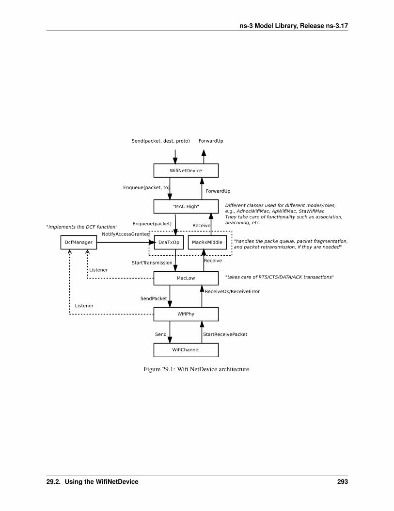
ns-3 Model Library, Release ns-3.17
Figure 29.1: Wifi NetDevice architecture.
29.2. Using the WifiNetDevice 293
ns-3 Model Library, Release ns-3.17
Users who use the low-level ns-3 API and who wish to add a WifiNetDevice to their node must create an in-stance of a WifiNetDevice, plus a number of constituent objects, and bind them together appropriately (the WifiNet-Device is very modular in this regard, for future extensibility). At the low-level API, this can be done withabout 20 lines of code (see ns3::WifiHelper::Install, and ns3::YansWifiPhyHelper::Create).They also must create, at some point, a WifiChannel, which also contains a number of constituent objects (seens3::YansWifiChannelHelper::Create).
However, a few helpers are available for users to add these devices and channels with only a few lines of code, if theyare willing to use defaults, and the helpers provide additional API to allow the passing of attribute values to changedefault values. The scripts in src/examples can be browsed to see how this is done.
29.2.1 YansWifiChannelHelper
The YansWifiChannelHelper has an unusual name. Readers may wonder why it is named this way. The reference isto the yans simulator from which this model is taken. The helper can be used to create a WifiChannel with a defaultPropagationLoss and PropagationDelay model. Specifically, the default is a channel model with a propagation delayequal to a constant, the speed of light, and a propagation loss based on a log distance model with a reference loss of46.6777 dB at reference distance of 1m.
Users will typically type code such as::
YansWifiChannelHelper wifiChannelHelper = YansWifiChannelHelper::Default ();Ptr<WifiChannel> wifiChannel = wifiChannelHelper.Create ();
to get the defaults. Note the distinction above in creating a helper object vs. an actual simulation object. In ns-3,helper objects (used at the helper API only) are created on the stack (they could also be created with operator new andlater deleted). However, the actual ns-3 objects typically inherit from class ns3::Object and are assigned to asmart pointer. See the chapter in the ns-3 manual for a discussion of the ns-3 object model, if you are not familiar withit.
Todo: Add notes about how to configure attributes with this helper API
29.2.2 YansWifiPhyHelper
Physical devices (base class ns3::Phy) connect to ns3::Channel models in ns-3. We need to create Phy objectsappropriate for the YansWifiChannel; here the YansWifiPhyHelper will do the work.
The YansWifiPhyHelper class configures an object factory to create instances of a YansWifiPhy and adds someother objects to it, including possibly a supplemental ErrorRateModel and a pointer to a MobilityModel. The usercode is typically::
YansWifiPhyHelper wifiPhyHelper = YansWifiPhyHelper::Default ();wifiPhyHelper.SetChannel (wifiChannel);
Note that we haven’t actually created any WifiPhy objects yet; we’ve just prepared the YansWifiPhyHelper by tellingit which channel it is connected to. The phy objects are created in the next step.
29.2.3 NqosWifiMacHelper and QosWifiMacHelper
The ns3::NqosWifiMacHelper and ns3::QosWifiMacHelper configure an object factory to create in-stances of a ns3::WifiMac. They are used to configure MAC parameters like type of MAC.
The former, ns3::NqosWifiMacHelper, supports creation of MAC instances that do not have 802.11e/WMM-style QoS support enabled.
294 Chapter 29. Wifi
ns-3 Model Library, Release ns-3.17
For example the following user code configures a non-QoS MAC that will be a non-AP STA in an infrastructurenetwork where the AP has SSID ns-3-ssid::
NqosWifiMacHelper wifiMacHelper = NqosWifiMacHelper::Default ();Ssid ssid = Ssid ("ns-3-ssid");wifiMacHelper.SetType ("ns3::StaWifiMac",
"Ssid", SsidValue (ssid),"ActiveProbing", BooleanValue (false));
To create MAC instances with QoS support enabled, ns3::QosWifiMacHelper is used in place ofns3::NqosWifiMacHelper. This object can be also used to set:
• a MSDU aggregator for a particular Access Category (AC) in order to use 802.11n MSDU aggregation feature;
• block ack parameters like threshold (number of packets for which block ack mechanism should be used) andinactivity timeout.
The following code shows an example use of ns3::QosWifiMacHelper to create an AP with QoS enabled,aggregation on AC_VO, and Block Ack on AC_BE::
QosWifiMacHelper wifiMacHelper = QosWifiMacHelper::Default ();wifiMacHelper.SetType ("ns3::ApWifiMac",
"Ssid", SsidValue (ssid),"BeaconGeneration", BooleanValue (true),"BeaconInterval", TimeValue (Seconds (2.5)));
wifiMacHelper.SetMsduAggregatorForAc (AC_VO, "ns3::MsduStandardAggregator","MaxAmsduSize", UintegerValue (3839));
wifiMacHelper.SetBlockAckThresholdForAc (AC_BE, 10);wifiMacHelper.SetBlockAckInactivityTimeoutForAc (AC_BE, 5);
29.2.4 WifiHelper
We’re now ready to create WifiNetDevices. First, let’s create a WifiHelper with default settings::
WifiHelper wifiHelper = WifiHelper::Default ();
What does this do? It sets the RemoteStationManager to ns3::ArfWifiManager. Now, let’s use the wifiPhy-Helper and wifiMacHelper created above to install WifiNetDevices on a set of nodes in a NodeContainer “c”::
NetDeviceContainer wifiContainer = WifiHelper::Install (wifiPhyHelper, wifiMacHelper, c);
This creates the WifiNetDevice which includes also a WifiRemoteStationManager, a WifiMac, and a WifiPhy (con-nected to the matching WifiChannel).
There are many ns-3 attributes that can be set on the above helpers to deviate from the default behavior; the examplescripts show how to do some of this reconfiguration.
29.2.5 AdHoc WifiNetDevice configuration
This is a typical example of how a user might configure an adhoc network.
To be completed
29.2.6 Infrastructure (Access Point and clients) WifiNetDevice configuration
This is a typical example of how a user might configure an access point and a set of clients.
To be completed
29.2. Using the WifiNetDevice 295
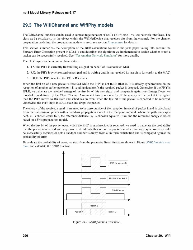
ns-3 Model Library, Release ns-3.17
29.3 The WifiChannel and WifiPhy models
The WifiChannel subclass can be used to connect together a set of ns3::WifiNetDevice network interfaces. Theclass ns3::WifiPhy is the object within the WifiNetDevice that receives bits from the channel. For the channelpropagation modeling, the propagation module is used; see section Propagation for details.
This section summarizes the description of the BER calculations found in the yans paper taking into account theForward Error Correction present in 802.11a and describes the algorithm we implemented to decide whether or not apacket can be successfully received. See “Yet Another Network Simulator” for more details.
The PHY layer can be in one of three states:
1. TX: the PHY is currently transmitting a signal on behalf of its associated MAC
2. RX: the PHY is synchronized on a signal and is waiting until it has received its last bit to forward it to the MAC.
3. IDLE: the PHY is not in the TX or RX states.
When the first bit of a new packet is received while the PHY is not IDLE (that is, it is already synchronized on thereception of another earlier packet or it is sending data itself), the received packet is dropped. Otherwise, if the PHY isIDLE, we calculate the received energy of the first bit of this new signal and compare it against our Energy Detectionthreshold (as defined by the Clear Channel Assessment function mode 1). If the energy of the packet k is higher,then the PHY moves to RX state and schedules an event when the last bit of the packet is expected to be received.Otherwise, the PHY stays in IDLE state and drops the packet.
The energy of the received signal is assumed to be zero outside of the reception interval of packet k and is calculatedfrom the transmission power with a path-loss propagation model in the reception interval. where the path loss expo-nent, n, is chosen equal to 3, the reference distance, d0 is choosen equal to 1.0m and the reference energy is basedbased on a Friis propagation model.
When the last bit of the packet upon which the PHY is synchronized is received, we need to calculate the probabilitythat the packet is received with any error to decide whether or not the packet on which we were synchronized couldbe successfully received or not: a random number is drawn from a uniform distribution and is compared against theprobability of error.
To evaluate the probability of error, we start from the piecewise linear functions shown in Figure SNIR function overtime. and calculate the SNIR function.
Figure 29.2: SNIR function over time.
296 Chapter 29. Wifi
ns-3 Model Library, Release ns-3.17
From the SNIR function we can derive the Bit Error Rate (BER) and Packet Error Rate (PER) for the modulation andcoding scheme being used for the transmission. Please refer to [pei80211ofdm], [pei80211b] and [lacage2006yans]for a detailed description of the available BER/PER models.
29.3.1 WifiChannel configuration
The WifiChannel implementation uses the propagation loss and delay models provided within the ns-3 propagationmodule.
29.4 The MAC model
The 802.11 Distributed Coordination Function is used to calculate when to grant access to the transmission medium.While implementing the DCF would have been particularly easy if we had used a recurring timer that expired everyslot, we chose to use the method described in [ji2004sslswn] where the backoff timer duration is lazily calculatedwhenever needed since it is claimed to have much better performance than the simpler recurring timer solution.
The backoff procedure of DCF is described in section 9.2.5.2 of [ieee80211].
• “The backoff procedure shall be invoked for a STA to transfer a frame when finding the medium busy as indi-cated by either the physical or virtual CS mechanism.”
• “A backoff procedure shall be performed immediately after the end of every transmission with the More Frag-ments bit set to 0 of an MPDU of type Data, Management, or Control with subtype PS-Poll, even if no additionaltransmissions are currently queued.”
Thus, if the queue is empty, a newly arrived packet should be transmitted immediately after channel is sensed idle forDIFS. If queue is not empty and after a successful MPDU that has no more fragments, a node should also start thebackoff timer.
Some users have observed that the 802.11 MAC with an empty queue on an idle channel will transmit the first framearriving to the model immediately without waiting for DIFS or backoff, and wonder whether this is compliant. Accord-ing to the standard, “The backoff procedure shall be invoked for a STA to transfer a frame when finding the mediumbusy as indicated by either the physical or virtual CS mechanism.” So in this case, the medium is not found to be busyin recent past and the station can transmit immediately.
The higher-level MAC functions are implemented in a set of other C++ classes and deal with:
• packet fragmentation and defragmentation,
• use of the rts/cts protocol,
• rate control algorithm,
• connection and disconnection to and from an Access Point,
• the MAC transmission queue,
• beacon generation,
• msdu aggregation,
• etc.
29.5 Wifi Attributes
Should link to the list of attributes exported by Doxygen
29.4. The MAC model 297

ns-3 Model Library, Release ns-3.17
29.6 Wifi Tracing
Should link to the list of traces exported by Doxygen
29.7 References
298 Chapter 29. Wifi
CHAPTER
THIRTY
WIMAX NETDEVICE
This chapter describes the ns-3 WimaxNetDevice and related models. By adding WimaxNetDevice objects to ns-3 nodes, one can create models of 802.16-based networks. Below, we list some more details about what the ns-3WiMAX models cover but, in summary, the most important features of the ns-3 model are:
• a scalable and realistic physical layer and channel model
• a packet classifier for the IP convergence sublayer
• efficient uplink and downlink schedulers
• support for Multicast and Broadcast Service (MBS), and
• packet tracing functionality
The source code for the WiMAX models lives in the directory src/wimax.
There have been two academic papers published on this model:
• M.A. Ismail, G. Piro, L.A. Grieco, and T. Turletti, “An Improved IEEE 802.16 WiMAX Module for the NS-3Simulator”, SIMUTools 2010 Conference, March 2010.
• J. Farooq and T. Turletti, “An IEEE 802.16 WiMAX module for the NS-3 Simulator,” SIMUTools 2009 Confer-ence, March 2009.
30.1 Scope of the model
From a MAC perspective, there are two basic modes of operation, that of a Subscriber Station (SS) or aBase Station (BS). These are implemented as two subclasses of the base class ns3::NetDevice, classSubscriberStationNetDevice and class BaseStationNetDevice. As is typical in ns-3, there is alsoa physical layer class WimaxPhy and a channel class WimaxChannel which serves to hold the references to all ofthe attached Phy devices. The main physical layer class is the SimpleOfdmWimaxChannel class.
Another important aspect of WiMAX is the uplink and downlink scheduler, and there are three primary schedulertypes implemented:
• SIMPLE: a simple priority based FCFS scheduler
• RTPS: a real-time polling service (rtPS) scheduler
• MBQOS: a migration-based uplink scheduler
The following additional aspects of the 802.16 specifications, as well as physical layer and channel models, are mod-elled:
• leverages existing ns-3 wireless propagation loss and delay models, as well as ns-3 mobility models
299
ns-3 Model Library, Release ns-3.17
• Point-to-Multipoint (PMP) mode and the WirelessMAN-OFDM PHY layer
• Initial Ranging
• Service Flow Initialization
• Management Connection
• Transport Initialization
• UGS, rtPS, nrtPS, and BE connections
The following aspects are not presently modelled but would be good topics for future extensions:
• OFDMA PHY layer
• Link adaptation
• Mesh topologies
• ARQ
• ertPS connection
• packet header suppression
30.2 Using the Wimax models
The main way that users who write simulation scripts will typically interact with the Wimax models is through thehelper API and through the publicly visible attributes of the model.
The helper API is defined in src/wimax/helper/wimax-helper.{cc,h}.
The example src/wimax/examples/wimax-simple.cc contains some basic code that shows how to set upthe model::
switch (schedType){case 0:scheduler = WimaxHelper::SCHED_TYPE_SIMPLE;break;
case 1:scheduler = WimaxHelper::SCHED_TYPE_MBQOS;break;
case 2:scheduler = WimaxHelper::SCHED_TYPE_RTPS;break;
default:scheduler = WimaxHelper::SCHED_TYPE_SIMPLE;
}
NodeContainer ssNodes;NodeContainer bsNodes;
ssNodes.Create (2);bsNodes.Create (1);
WimaxHelper wimax;
NetDeviceContainer ssDevs, bsDevs;
ssDevs = wimax.Install (ssNodes,
300 Chapter 30. Wimax NetDevice
ns-3 Model Library, Release ns-3.17
WimaxHelper::DEVICE_TYPE_SUBSCRIBER_STATION,WimaxHelper::SIMPLE_PHY_TYPE_OFDM,scheduler);
bsDevs = wimax.Install (bsNodes, WimaxHelper::DEVICE_TYPE_BASE_STATION, WimaxHelper::SIMPLE_PHY_TYPE_OFDM, scheduler);
This example shows that there are two subscriber stations and one base station created. The helper method Installallows the user to specify the scheduler type, the physical layer type, and the device type.
Different variants of Install are available; for instance, the examplesrc/wimax/examples/wimax-multicast.cc shows how to specify a non-default channel or propa-gation model::
channel = CreateObject<SimpleOfdmWimaxChannel> ();channel->SetPropagationModel (SimpleOfdmWimaxChannel::COST231_PROPAGATION);ssDevs = wimax.Install (ssNodes,
WimaxHelper::DEVICE_TYPE_SUBSCRIBER_STATION,WimaxHelper::SIMPLE_PHY_TYPE_OFDM,channel,scheduler);
Ptr<WimaxNetDevice> dev = wimax.Install (bsNodes.Get (0),WimaxHelper::DEVICE_TYPE_BASE_STATION,WimaxHelper::SIMPLE_PHY_TYPE_OFDM,channel,scheduler);
Mobility is also supported in the same way as in Wifi models; see thesrc/wimax/examples/wimax-multicast.cc.
Another important concept in WiMAX is that of a service flow. This is a unidirectional flow of packets witha set of QoS parameters such as traffic priority, rate, scheduling type, etc. The base station is responsi-ble for issuing service flow identifiers and mapping them to WiMAX connections. The following code fromsrc/wimax/examples/wimax-multicast.cc shows how this is configured from a helper level::
ServiceFlow MulticastServiceFlow = wimax.CreateServiceFlow (ServiceFlow::SF_DIRECTION_DOWN,ServiceFlow::SF_TYPE_UGS,MulticastClassifier);
bs->GetServiceFlowManager ()->AddMulticastServiceFlow (MulticastServiceFlow, WimaxPhy::MODULATION_TYPE_QPSK_12);
30.3 Wimax Attributes
The WimaxNetDevice makes heavy use of the ns-3 attributes subsystem for configuration and default value manage-ment. Presently, approximately 60 values are stored in this system.
For instance, class ns-3::SimpleOfdmWimaxPhy exports these attributes:
• NoiseFigure: Loss (dB) in the Signal-to-Noise-Ratio due to non-idealities in the receiver.
• TxPower: Transmission power (dB)
• G: The ratio of CP time to useful time
• txGain: Transmission gain (dB)
• RxGain: Reception gain (dB)
• Nfft: FFT size
• TraceFilePath: Path to the directory containing SNR to block error rate files
30.3. Wimax Attributes 301
ns-3 Model Library, Release ns-3.17
For a full list of attributes in these models, consult the Doxygen page that lists all attributes for ns-3.
30.4 Wimax Tracing
ns-3 has a sophisticated tracing infrastructure that allows users to hook into existing trace sources, or to define andexport new ones.
Many ns-3 users use the built-in Pcap or Ascii tracing, and the WimaxHelper has similar APIs::
AsciiTraceHelper ascii;WimaxHelper wimax;wimax.EnablePcap ("wimax-program", false);wimax.EnableAsciiAll (ascii.CreateFileStream ("wimax-program.tr");
Unlike other helpers, there is also a special EnableAsciiForConnection() method that limits the ascii tracingto a specific device and connection.
These helpers access the low level trace sources that exist in the WiMAX physical layer, net device, and queue models.Like other ns-3 trace sources, users may hook their own functions to these trace sources if they want to do customizedthings based on the packet events. See the Doxygen List of trace sources for a complete list of these sources.
30.5 Wimax MAC model
The 802.16 model provided in ns-3 attempts to provide an accurate MAC and PHY level implementation of the 802.16specification with the Point-to-Multipoint (PMP) mode and the WirelessMAN-OFDM PHY layer. The model is mainlycomposed of three layers:
• The convergence sublayer (CS)
• The MAC CP Common Part Sublayer (MAC-CPS)
• Physical (PHY) layer
The following figure WiMAX architecture shows the relationships of these models.
30.5.1 Convergence Sublayer
The Convergence sublayer (CS) provided with this module implements the Packet CS, designed to work with thepacket-based protocols at higher layers. The CS is responsible of receiving packet from the higher layer and frompeer stations, classifying packets to appropriate connections (or service flows) and processing packets. It keeps amapping of transport connections to service flows. This enables the MAC CPS identifying the Quality of Service(QoS) parameters associated to a transport connection and ensuring the QoS requirements. The CS currently employsan IP classifier.
30.5.2 IP Packet Classifier
An IP packet classifier is used to map incoming packets to appropriate connections based on a set of criteria. Theclassifier maintains a list of mapping rules which associate an IP flow (src IP address and mask, dst IP address andmask, src port range, dst port range and protocol) to one of the service flows. By analyzing the IP and the TCP/UDPheaders the classifier will append the incoming packet (from the upper layer) to the queue of the appropriate WiMAXconnection. Class IpcsClassifier and class IpcsClassifierRecord implement the classifier module forboth SS and BS
302 Chapter 30. Wimax NetDevice
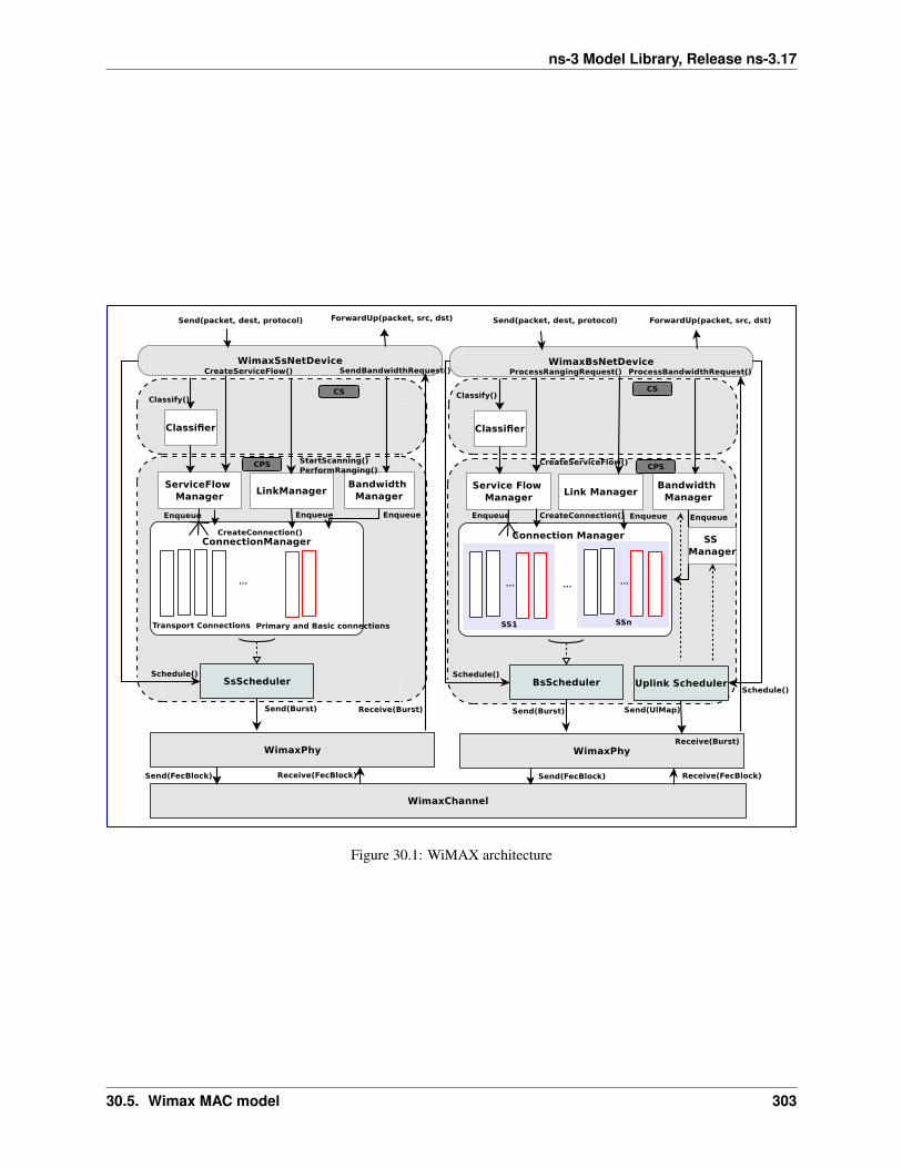
ns-3 Model Library, Release ns-3.17
Figure 30.1: WiMAX architecture
30.5. Wimax MAC model 303
ns-3 Model Library, Release ns-3.17
30.5.3 MAC Common Part Sublayer
The MAC Common Part Sublayer (CPS) is the main sublayer of the IEEE 802.16 MAC and performs the fundamentalfunctions of the MAC. The module implements the Point-Multi-Point (PMP) mode. In PMP mode BS is respon-sible of managing communication among multiple SSs. The key functionalities of the MAC CPS include framingand addressing, generation of MAC management messages, SS initialization and registration, service flow manage-ment, bandwidth management and scheduling services. Class WimaxNetDevice represents the MAC layer of aWiMAX network device. This class extends the class NetDevice of the ns-3 API that provides abstraction ofa network device. Class WimaxNetDevice is further extended by class BaseStationNetDevice and classSubscriberStationNetDevice, defining MAC layers of BS and SS, respectively. Besides these main classes,the key functions of MAC are distributed to several other classes.
30.5.4 Framing and Management Messages
The module implements a frame as a fixed duration of time, i.e., frame boundaries are defined with respect to time.Each frame is further subdivided into downlink (DL) and uplink (UL) subframes. The module implements the TimeDivision Duplex (TDD) mode where DL and UL operate on same frequency but are separated in time. A number ofDL and UL bursts are then allocated in DL and UL subframes, respectively. Since the standard allows sending andreceiving bursts of packets in a given DL or UL burst, the unit of transmission at the MAC layer is a packet burst. Themodule implements a special PacketBurst data structure for this purpose. A packet burst is essentially a list of packets.The BS downlink and uplink schedulers, implemented by class BSScheduler and class UplinkScheduler,are responsible of generating DL and UL subframes, respectively. In the case of DL, the subframe is simulated bytransmitting consecutive bursts (instances PacketBurst). In case of UL, the subframe is divided, with respect to time,into a number of slots. The bursts transmitted by the SSs in these slots are then aligned to slot boundaries. The frame isdivided into integer number of symbols and Physical Slots (PS) which helps in managing bandwidth more effectively.The number of symbols per frame depends on the underlying implementation of the PHY layer. The size of a DL orUL burst is specified in units of symbols.
30.5.5 Network Entry and Initialization
The network entry and initialization phase is basically divided into two sub-phases, (1) scanning and synchronizationand (2) initial ranging. The entire phase is performed by the LinkManager component of SS and BS. Once an SSwants to join the network, it first scans the downlink frequencies to search for a suitable channel. The search iscomplete as soon as it detects a PHY frame. The next step is to establish synchronization with the BS. Once SSreceives a Downlink-MAP (DL-MAP) message the synchronization phase is complete and it remains synchronized aslong as it keeps receiving DL-MAP and Downlink Channel Descriptor (DCD) messages. After the synchronization isestablished, SS waits for a Uplink Channel Descriptor (UCD) message to acquire uplink channel parameters. Onceacquired, the first sub-phase of the network entry and initialization is complete. Once synchronization is achieved, theSS waits for a UL-MAP message to locate a special grant, called initial ranging interval, in the UL subframe. Thisgrant is allocated by the BS Uplink Scheduler at regular intervals. Currently this interval is set to 0.5 ms, however theuser is enabled to modify its value from the simulation script.
30.5.6 Connections and Addressing
All communication at the MAC layer is carried in terms of connections. The standard defines a connection as aunidirectional mapping between the SS and BS’s MAC entities for the transmission of traffic. The standard defines twotypes of connections: management connections for transmitting control messages and transport connections for datatransmission. A connection is identified by a 16-bit Connection Identifier (CID). Class WimaxConnection and classCid implement the connection and CID, respectively. Note that each connection maintains its own transmission queuewhere packets to transmit on that connection are queued. The ConnectionManager component of BS is responsible ofcreating and managing connections for all SSs.
304 Chapter 30. Wimax NetDevice
ns-3 Model Library, Release ns-3.17
The two key management connections defined by the standard, namely the Basic and Primary management con-nections, are created and allocated to the SS during the ranging process. Basic connection plays an important rolethroughout the operation of SS also because all (unicast) DL and UL grants are directed towards SS’s Basic CID. Inaddition to management connections, an SS may have one or more transport connections to send data packets. TheConnection Manager component of SS manages the connections associated to SS. As defined by the standard, a man-agement connection is bidirectional, i.e., a pair of downlink and uplink connections is represented by the same CID.This feature is implemented in a way that one connection (in DL direction) is created by the BS and upon receivingthe CID the SS then creates an identical connection (in UL direction) with the same CID.
30.5.7 Scheduling Services
The module supports the four scheduling services defined by the 802.16-2004 standard:
• Unsolicited Grant Service (UGS)
• Real-Time Polling Services (rtPS)
• Non Real-Time Polling Services (nrtPS)
• Best Effort (BE)
These scheduling services behave differently with respect to how they request bandwidth as well as how the it isgranted. Each service flow is associated to exactly one scheduling service, and the QoS parameter set associated to aservice flow actually defines the scheduling service it belongs to. When a service flow is created the UplinkSchedulercalculates necessary parameters such as grant size and grant interval based on QoS parameters associated to it.
30.5.8 WiMAX Uplink Scheduler Model
Uplink Scheduler at the BS decides which of the SSs will be assigned uplink allocations based on the QoS parametersassociated to a service flow (or scheduling service) and bandwidth requests from the SSs. Uplink scheduler togetherwith Bandwidth Manager implements the complete scheduling service functionality. The standard defines up to fourscheduling services (BE, UGS, rtPS, nrtPS) for applications with different types of QoS requirements. The serviceflows of these scheduling services behave differently with respect to how they request for bandwidth as well as howthe bandwidth is granted. The module supports all four scheduling services. Each service flow is associated to exactlyone transport connection and one scheduling service. The QoS parameters associated to a service flow actually definethe scheduling service it belongs to. Standard QoS parameters for UGS, rtPS, nrtPS and BE services, as specified inTables 111a to 111d of the 802.16e amendment, are supported. When a service flow is created the uplink schedulercalculates necessary parameters such as grant size and allocation interval based on QoS parameters associated to it.The current WiMAX module provides three different versions of schedulers.
• The first one is a simple priority-based First Come First Serve (FCFS). For the real-time services (UGS andrtPS) the BS then allocates grants/polls on regular basis based on the calculated interval. For the non real-timeservices (nrtPS and BE) only minimum reserved bandwidth is guaranteed if available after servicing real-timeflows. Note that not all of these parameters are utilized by the uplink scheduler. Also note that currently onlyservice flow with fixed-size packet size are supported, as currently set up in simulation scenario with OnOffapplication of fixed packet size. This scheduler is implemented by class BSSchedulerSimple and classUplinkSchedulerSimple.
• The second one is similar to first scheduler except by rtPS service flow. All rtPS Connections are able totransmit all packet in the queue according to the available bandwidth. The bandwidth saturation control hasbeen implemented to redistribute the effective available bandwidth to all rtPS that have at least one packet totransmit. The remaining bandwidth is allocated to nrtPS and BE Connections. This scheduler is implementedby class BSSchedulerRtps and class UplinkSchedulerRtps.
• The third one is a Migration-based Quality of Service uplink scheduler This uplink scheduler uses three queues,the low priority queue, the intermediate queue and the high priority queue. The scheduler serves the requests
30.5. Wimax MAC model 305
ns-3 Model Library, Release ns-3.17
in strict priority order from the high priority queue to the low priority queue. The low priority queue stores thebandwidth requests of the BE service flow. The intermediate queue holds bandwidth requests sent by rtPS andby nrtPS connections. rtPS and nrtPS requests can migrate to the high priority queue to guarantee that their QoSrequirements are met. Besides the requests migrated from the intermediate queue, the high priority queue storesperiodic grants and unicast request opportunities that must be scheduled in the following frame. To guaranteethe maximum delay requirement, the BS assigns a deadline to each rtPS bandwidth request in the intermediatequeue. The minimum bandwidth requirement of both rtPS and nrtPS connections is guaranteed over a windowof duration T. This scheduler is implemented by class UplinkSchedulerMBQoS.
30.5.9 WiMAX Outbound Schedulers Model
Besides the uplink scheduler these are the outbound schedulers at BS and SS side (BSScheduler and SSScheduler). Theoutbound schedulers decide which of the packets from the outbound queues will be transmitted in a given allocation.The outbound scheduler at the BS schedules the downlink traffic, i.e., packets to be transmitted to the SSs in thedownlink subframe. Similarly the outbound scheduler at a SS schedules the packet to be transmitted in the uplinkallocation assigned to that SS in the uplink subframe. All three schedulers have been implemented to work as FCFSscheduler, as they allocate grants starting from highest priority scheduling service to the lower priority one (UGS>rtPS> nrtPS> BE). The standard does not suggest any scheduling algorithm and instead leaves this decision up to themanufacturers. Of course more sophisticated algorithms can be added later if required.
30.6 WimaxChannel and WimaxPhy models
The module implements the Wireless MAN OFDM PHY specifications as the more relevant for implementation as itis the schema chosen by the WiMAX Forum. This specification is designed for non-light-of-sight (NLOS) includingfixed and mobile broadband wireless access. The proposed model uses a 256 FFT processor, with 192 data subcarriers.It supports all the seven modulation and coding schemes specified by Wireless MAN-OFDM. It is composed of twoparts: the channel model and the physical model.
30.7 Channel model
The channel model we propose is implemented by the class SimpleOFDMWimaxChannel which extends the classwimaxchannel. The channel entity has a private structure named m_phyList which handles all the physical devicesconnected to it. When a physical device sends a packet (FEC Block) to the channel, the channel handles the packet,and then for each physical device connected to it, it calculates the propagation delay, the path loss according to agiven propagation model and eventually forwards the packet to the receiver device. The channel class uses the methodGetDistanceFrom() to calculate the distance between two physical entities according to their 3D coordinates. Thedelay is computed as delay = distance/C, where C is the speed of the light.
30.8 Physical model
The physical layer performs two main operations: (i) It receives a burst from a channel and forwards it to the MAClayer, (ii) it receives a burst from the MAC layer and transmits it on the channel. In order to reduce the simulationcomplexity of the WiMAX physical layer, we have chosen to model offline part of the physical layer. More specificallywe have developed an OFDM simulator to generate trace files used by the reception process to evaluate if a FEC blockcan be correctly decoded or not.
Transmission Process: A burst is a set of WiMAX MAC PDUs. At the sending process, a burst is converted intobit-streams and then splitted into smaller FEC blocks which are then sent to the channel with a power equal P_tx.
306 Chapter 30. Wimax NetDevice
ns-3 Model Library, Release ns-3.17
Reception Process: The reception process includes the following operations:
1. Receive a FEC block from the channel.
2. Calculate the noise level.
3. Estimate the signal to noise ratio (SNR) with the following formula.
4. Determine if a FEC block can be correctly decoded.
5. Concatenate received FEC blocks to reconstruct the original burst.
6. Forward the burst to the upper layer.
The developed process to evaluate if a FEC block can be correctly received or not uses pre-generated traces. The tracefiles are generated by an external OFDM simulator (described later). A class named SNRToBlockErrorRateManagerhandles a repository containing seven trace files (one for each modulation and coding scheme). A repository is specificfor a particular channel model.
A trace file is made of 6 columns. The first column provides the SNR value (1), whereas the other columns giverespectively the bit error rate BER (2), the block error rate BlcER(3), the standard deviation on BlcER, and theconfidence interval (4 and 5). These trace files are loaded into memory by the SNRToBlockErrorRateManager entityat the beginning of the simulation.
Currently, The first process uses the first and third columns to determine if a FEC block is correctly received. When thephysical layer receives a packet with an SNR equal to SNR_rx, it asks the SNRToBlockErrorRateManager to returnthe corresponding block error rate BlcER. A random number RAND between 0 and 1 is then generated. If RAND isgreater than BlcER, then the block is correctly received, otherwise the block is considered erroneous and is ignored.
The module provides defaults SNR to block error rate traces in default-traces.h. The traces have been generated by anExternal WiMAX OFDM simulator. The simulator is based on an external mathematics and signal processing libraryIT++ and includes : a random block generator, a Reed Solomon (RS) coder, a convolutional coder, an interleaver, a256 FFT-based OFDM modulator, a multi-path channel simulator and an equalizer. The multipath channel is simulatedusing the TDL_channel class of the IT++ library.
Users can configure the module to use their own traces generated by another OFDM simulator or ideally by performingexperiments in real environment. For this purpose, a path to a repository containing trace files should be provided. Ifno repository is provided the traces form default-traces.h will be loaded. A valid repository should contain 7 files, onefor each modulation and coding scheme.
The names of the files should respect the following format: modulation0.txt for modulation 0, modulation1.txt formodulation 1 and so on... The file format should be as follows:
SNR_value1 BER Blc_ER STANDARD_DEVIATION CONFIDENCE_INTERVAL1 CONFIDENCE_INTERVAL2SNR_value2 BER Blc_ER STANDARD_DEVIATION CONFIDENCE_INTERVAL1 CONFIDENCE_INTERVAL2... ... ... ... ... ...... ... ... ... ... ...
30.8. Physical model 307

ns-3 Model Library, Release ns-3.17
308 Chapter 30. Wimax NetDevice

BIBLIOGRAPHY
[Balanis] C.A. Balanis, “Antenna Theory - Analysis and Design”, Wiley, 2nd Ed.
[Chunjian] Li Chunjian, “Efficient Antenna Patterns for Three-Sector WCDMA Systems”, Master of Science Thesis,Chalmers University of Technology, Göteborg, Sweden, 2003
[Calcev] George Calcev and Matt Dillon, “Antenna Tilt Control in CDMA Networks”, in Proc. of the 2nd AnnualInternational Wireless Internet Conference (WICON), 2006
[R4-092042a] 3GPP TSG RAN WG4 (Radio) Meeting #51, R4-092042, Simulation assumptions and parameters forFDD HeNB RF requirements.
[rfc3561] RFC 3561 Ad hoc On-Demand Distance Vector (AODV) Routing
[turkmani] Turkmani A.M.D., J.D. Parson and D.G. Lewis, “Radio propagation into buildings at 441, 900 and 1400MHz”, in Proc. of 4th Int. Conference on Land Mobile Radio, 1987.
[TS25814] 3GPP TS 25.814 “Physical layer aspect for evolved Universal Terrestrial Radio Access”
[TS29274] 3GPP TS 29.274 “Tunnelling Protocol for Control plane (GTPv2-C)”
[TS36101] 3GPP TS 36.101 “E-UTRA User Equipment (UE) radio transmission and reception”
[TS36104] 3GPP TS 36.104 “E-UTRA Base Station (BS) radio transmission and reception”
[TS36211] 3GPP TS 36.211 “E-UTRA Physical Channels and Modulation”
[TS36212] 3GPP TS 36.212 “E-UTRA Multiplexing and channel coding”
[TS36213] 3GPP TS 36.213 “E-UTRA Physical layer procedures”
[TS36300] 3GPP TS 36.300 “E-UTRA and E-UTRAN; Overall description; Stage 2”
[TS36304] 3GPP TS 36.104 “E-UTRA User Equipment (UE) procedures in idle mode”
[TS36321] 3GPP TS 36.321 “E-UTRA Medium Access Control (MAC) protocol specification”
[TS36322] 3GPP TS 36.322 “E-UTRA Radio Link Control (RLC) protocol specification”
[TS36323] 3GPP TS 36.323 “E-UTRA Packet Data Convergence Protocol (PDCP) specification”
[TS36331] 3GPP TS 36.331 “E-UTRA Radio Resource Control (RRC) protocol specification”
[TS36413] 3GPP TS 36.413 “E-UTRAN S1 application protocol (S1AP)”
[TS36420] 3GPP TS 36.420 “E-UTRAN X2 general aspects and principles”
[TS36423] 3GPP TS 36.423 “E-UTRAN X2 application protocol (X2AP)”
[R1-081483] 3GPP R1-081483 Conveying MCS and TB size via PDCCH
309
ns-3 Model Library, Release ns-3.17
[R4-092042] 3GPP R4-092042 “Simulation assumptions and parameters for FDD HeNB RF requirements”
[TR36814] 3GPP TR 36.814 “E-UTRA Further advancements for E-UTRA physical layer aspects”
[FFAPI] FemtoForum LTE MAC Scheduler Interface Specification v1.11
[ns3tutorial] The ns-3 Tutorial
[ns3manual] The ns-3 Manual
[Sesia2009] S. Sesia, I. Toufik and M. Baker, “LTE - The UMTS Long Term Evolution - from theory to practice”,Wiley, 2009
[Baldo2009] N. Baldo and M. Miozzo, “Spectrum-aware Channel and PHY layer modeling for ns3”, Proceedings ofICST NSTools 2009, Pisa, Italy.
[Piro2010] Giuseppe Piro, Luigi Alfredo Grieco, Gennaro Boggia, and Pietro Camarda, A Two-level SchedulingAlgorithm for QoS Support in the Downlink of LTE Cellular Networks”, Proc. of European Wireless, EW2010,Lucca, Italy, Apr., 2010
[Holtzman2000] J.M. Holtzman, “CDMA forward link waterfilling power control”, in Proc. of IEEE VTC Spring,2000.
[Piro2011] G. Piro, N. Baldo. M. Miozzo, “An LTE module for the ns-3 network simulator”, in Proc. of Wns3 2011(in conjunction with SimuTOOLS 2011), March 2011, Barcelona (Spain)
[Seo2004] H. Seo, B. G. Lee. “A proportional-fair power allocation scheme for fair and efficient multiuser OFDMsystems”, in Proc. of IEEE GLOBECOM, December 2004. Dallas (USA)
[Ofcom2600MHz] Ofcom, “Consultation on assessment of future mobile competition and proposals for the award of800 MHz and 2.6 GHz spectrum and related issues”, March 2011
[RealWireless] RealWireless, Low-power shared access to spectrum for mobile broadband, Final Report, OfcomProject MC/073, 18th March 2011
[PaduaPEM] http://mailman.isi.edu/pipermail/ns-developers/2011-November/009559.html
[ViennaLteSim] The Vienna LTE Simulators http://www.nt.tuwien.ac.at/about-us/staff/josep-colom-ikuno/lte-simulators/
[LozanoCost] Joan Olmos, Silvia Ruiz, Mario García-Lozano and David Martín-Sacristán, “Link Abstraction ModelsBased on Mutual Information for LTE Downlink”, COST 2100 TD(10)11052 Report
[wimaxEmd] WiMAX Forum White Paper, WiMAX System Evaluation Methodology, July 2008.
[mathworks] Matlab R2011b Documentation Communications System Toolbox, Methodology for Simulating Multi-path Fading Channels
[CatreuxMIMO] 19. Catreux, L.J. Greenstein, V. Erceg, “Some results and insights on the performance gains ofMIMO systems,” Selected Areas in Communications, IEEE Journal on , vol.21, no.5, pp. 839- 847, June2003
[Ikuno2010] J.C. Ikuno, M. Wrulich, M. Rupp, “System Level Simulation of LTE Networks,” Vehicular TechnologyConference (VTC 2010-Spring), 2010 IEEE 71st , vol., no., pp.1-5, 16-19 May 2010
[Milos2012] 10. Milos, “Performace Analysis Of PCFICH LTE Control Channel”, Proceedings of the 19th Confer-ence STUDENT EEICT 2012, Brno, CZ, 2012.
[FujitsuWhitePaper] “Enhancing LTE Cell-Edge Performance via PDCCH ICIC”.
[Bharucha2011] 26. Bharucha, G. Auer, T. Abe, N. Miki, “Femto-to-Macro Control Channel Interference Mitigationvia Cell ID Manipulation in LTE,” Vehicular Technology Conference (VTC Fall), 2011 IEEE , vol., no., pp.1-6, 5-8 Sept. 2011
310 Bibliography
ns-3 Model Library, Release ns-3.17
[R4-081920] 3GPP R4-081920 LTE PDCCH/PCFICH Demodulation Performance Results with Implementation Mar-gin
[FCapo2012] F.Capozzi, G.Piro L.A.Grieco, G.Boggia, P.Camarda, “Downlink Packet Scheduling in LTE CellularNetworks: Key Design Issues and a Survey”, IEEE Comm. Surveys and Tutorials, vol.2012, no.99, pp.1-23, Jun.2012
[FABokhari2009] F.A. Bokhari, H. Yanikomeroglu, W.K. Wong, M. Rahman, “Cross-Layer Resource Scheduling forVideo Traffic in the Downlink of OFDMA-Based Wireless 4G Networks”,EURASIP J. Wirel. Commun. Netw.,vol.2009, no.3, pp. 1-10, Jan. 2009.
[WKWong2004] W.K. Wong, H.Y. Tang, V.C.M, Leung, “Token bank fair queuing: a new scheduling algorithm forwireless multimedia services”, Int. J. Commun. Syst., vol.17, no.6, pp.591-614, Aug.2004.
[GMonghal2008] G.Mongha, K.I. Pedersen, I.Z. Kovacs, P.E. Mogensen, ” QoS Oriented Time and Frequency Do-main Packet Schedulers for The UTRAN Long Term Evolution”, In Proc. IEEE VTC, 2008.
[rfc3626] RFC 3626 Optimized Link State Routing
[hata] M.Hata, “Empirical formula for propagation loss in land mobile radio services”, IEEE Trans. on VehicularTechnology, vol. 29, pp. 317-325, 1980
[cost231] “Digital Mobile Radio: COST 231 View on the Evolution Towards 3rd Generation Systems”, Commissionof the European Communities, L-2920, Luxembourg, 1989
[walfisch] J.Walfisch and H.L. Bertoni, “A Theoretical model of UHF propagation in urban environments,” in IEEETrans. Antennas Propagat., vol.36, 1988, pp.1788- 1796
[ikegami] F.Ikegami, T.Takeuchi, and S.Yoshida, “Theoretical prediction of mean field strength for Urban MobileRadio”, in IEEE Trans. Antennas Propagat., Vol.39, No.3, 1991
[kun2600mhz] Sun Kun, Wang Ping, Li Yingze, “Path loss models for suburban scenario at 2.3GHz, 2.6GHz and3.5GHz”, in Proc. of the 8th International Symposium on Antennas, Propagation and EM Theory (ISAPE), Kun-ming, China, Nov 2008.
[ieee80211] IEEE Std 802.11-2007 Wireless LAN Medium Access Control (MAC) and Physical Layer (PHY) Specifi-cations
[pei80211b] G. Pei and Tom Henderson, Validation of ns-3 802.11b PHY model
[pei80211ofdm] G. Pei and Tom Henderson, Validation of OFDM error rate model in ns-3
[lacage2006yans] M. Lacage and T. Henderson, Yet another Network Simulator
[ji2004sslswn] Z. Ji, J. Zhou, M. Takai and R. Bagrodia, Scalable simulation of large-scale wireless networks withbounded inaccuracies, in Proc. of the Seventh ACM Symposium on Modeling, Analysis and Simulation of Wire-less and Mobile Systems, October 2004.
Bibliography 311