ntrbtn t th pr f n rth* n. - hong kong university of ...ihome.ust.hk/~dxie/econ5250/mrw qje...
TRANSCRIPT
A CONTRIBUTION TO THE EMPIRICS OFECONOMIC GROWTH*
N. GREGORY MANKIW
DAVID ROMER
DAVID N. WEIL
This paper examines whether the Solow growth model is consistent with theinternational variation in the standard of living. It shows that an augmented Solowmodel that includes accumulation of human as well as physical capital provides anexcellent description of the cross-country data. The paper also examines theimplications of the Solow model for convergence in standards of living, that is, forwhether poor countries tend to grow faster than rich countries. The evidenceindicates that, holding population growth and capital accumulation constant,countries converge at about the rate the augmented Solow model predicts.
INTRODUCTION
This paper takes Robert Solow seriously. In his classic 1956article Solow proposed that we begin the study of economic growthby assuming a standard neoclassical production function withdecreasing returns to capital. Taking the rates of saving andpopulation growth as exogenous, he showed that these two vari-ables determine the steady-state level of income per capita. Be-cause saving and population growth rates vary across countries,different countries reach different steady states. Solow's modelgives simple testable predictions about how these variables influ-ence the steady-state level of income. The higher the rate of saving,the richer the country. The higher the rate of population growth,the poorer the country.
This paper argues that the predictions of the Solow model are,to a first approximation, consistent with the evidence. Examiningrecently available data for a large set of countries, we find thatsaving and population growth affect income in the directions thatSolow predicted. Moreover, more than half of the cross-countryvariation in income per capita can be explained by these twovariables alone.
Yet all is not right for the Solow model. Although the modelcorrectly predicts the directions of the effects of saving and
*We are grateful to Karen Dynan for research assistance, to Laurence Ball,Olivier Blanchard, Anne Case, Lawrence Katz, Robert King, Paul Romer, XavierSala-i-Martin, Amy Salsbury, Robert Solow, Lawrence Summers, Peter Temin, andthe referees for helpful comments, and to the National Science Foundation forfinancial support.
1992 by the President and Fellows of Harvard College and the Massachusetts Institute ofTechnology.The Quarterly Journal of Economics, May 1992
at Hong K
ong University of Science &
Technology on Septem
ber 22, 2013http://qje.oxfordjournals.org/
Dow
nloaded from
at Hong K
ong University of Science &
Technology on Septem
ber 22, 2013http://qje.oxfordjournals.org/
Dow
nloaded from
at Hong K
ong University of Science &
Technology on Septem
ber 22, 2013http://qje.oxfordjournals.org/
Dow
nloaded from
at Hong K
ong University of Science &
Technology on Septem
ber 22, 2013http://qje.oxfordjournals.org/
Dow
nloaded from
at Hong K
ong University of Science &
Technology on Septem
ber 22, 2013http://qje.oxfordjournals.org/
Dow
nloaded from
at Hong K
ong University of Science &
Technology on Septem
ber 22, 2013http://qje.oxfordjournals.org/
Dow
nloaded from
at Hong K
ong University of Science &
Technology on Septem
ber 22, 2013http://qje.oxfordjournals.org/
Dow
nloaded from
at Hong K
ong University of Science &
Technology on Septem
ber 22, 2013http://qje.oxfordjournals.org/
Dow
nloaded from
at Hong K
ong University of Science &
Technology on Septem
ber 22, 2013http://qje.oxfordjournals.org/
Dow
nloaded from
at Hong K
ong University of Science &
Technology on Septem
ber 22, 2013http://qje.oxfordjournals.org/
Dow
nloaded from
at Hong K
ong University of Science &
Technology on Septem
ber 22, 2013http://qje.oxfordjournals.org/
Dow
nloaded from
at Hong K
ong University of Science &
Technology on Septem
ber 22, 2013http://qje.oxfordjournals.org/
Dow
nloaded from
at Hong K
ong University of Science &
Technology on Septem
ber 22, 2013http://qje.oxfordjournals.org/
Dow
nloaded from
at Hong K
ong University of Science &
Technology on Septem
ber 22, 2013http://qje.oxfordjournals.org/
Dow
nloaded from
at Hong K
ong University of Science &
Technology on Septem
ber 22, 2013http://qje.oxfordjournals.org/
Dow
nloaded from
at Hong K
ong University of Science &
Technology on Septem
ber 22, 2013http://qje.oxfordjournals.org/
Dow
nloaded from
at Hong K
ong University of Science &
Technology on Septem
ber 22, 2013http://qje.oxfordjournals.org/
Dow
nloaded from
at Hong K
ong University of Science &
Technology on Septem
ber 22, 2013http://qje.oxfordjournals.org/
Dow
nloaded from
at Hong K
ong University of Science &
Technology on Septem
ber 22, 2013http://qje.oxfordjournals.org/
Dow
nloaded from
at Hong K
ong University of Science &
Technology on Septem
ber 22, 2013http://qje.oxfordjournals.org/
Dow
nloaded from
at Hong K
ong University of Science &
Technology on Septem
ber 22, 2013http://qje.oxfordjournals.org/
Dow
nloaded from
at Hong K
ong University of Science &
Technology on Septem
ber 22, 2013http://qje.oxfordjournals.org/
Dow
nloaded from
at Hong K
ong University of Science &
Technology on Septem
ber 22, 2013http://qje.oxfordjournals.org/
Dow
nloaded from
at Hong K
ong University of Science &
Technology on Septem
ber 22, 2013http://qje.oxfordjournals.org/
Dow
nloaded from
at Hong K
ong University of Science &
Technology on Septem
ber 22, 2013http://qje.oxfordjournals.org/
Dow
nloaded from
at Hong K
ong University of Science &
Technology on Septem
ber 22, 2013http://qje.oxfordjournals.org/
Dow
nloaded from
at Hong K
ong University of Science &
Technology on Septem
ber 22, 2013http://qje.oxfordjournals.org/
Dow
nloaded from
at Hong K
ong University of Science &
Technology on Septem
ber 22, 2013http://qje.oxfordjournals.org/
Dow
nloaded from
at Hong K
ong University of Science &
Technology on Septem
ber 22, 2013http://qje.oxfordjournals.org/
Dow
nloaded from
at Hong K
ong University of Science &
Technology on Septem
ber 22, 2013http://qje.oxfordjournals.org/
Dow
nloaded from
at Hong K
ong University of Science &
Technology on Septem
ber 22, 2013http://qje.oxfordjournals.org/
Dow
nloaded from
408 QUARTERLY JOURNAL OF ECONOMICS
population growth, it does not correctly predict the magnitudes. Inthe data the effects of saving and population growth on income aretoo large. To understand the relation between saving, populationgrowth, and income, one must go beyond the textbook Solowmodel.
We therefore augment the Solow model by including accumu-lation of human as well as physical capital. The exclusion of humancapital from the textbook Solow model can potentially explain whythe estimated influences of saving and population growth appeartoo large, for two reasons. First, for any given rate of human-capital accumulation, higher saving or lower population growthleads to a higher level of income and thus a higher level of humancapital; hence, accumulation of physical capital and populationgrowth have greater impacts on income when accumulation ofhuman capital is taken into account. Second, human-capital accu-mulation may be correlated with saving rates and populationgrowth rates; this would imply that omitting human-capital accu-mulation biases the estimated coefficients on saving and populationgrowth.
To test the augmented Solow model, we include a proxy forhuman-capital accumulation as an additional explanatory variablein our cross-country regressions. We find that accumulation ofhuman capital is in fact correlated with saving and populationgrowth. Including human-capital accumulation lowers the esti-mated effects of saving and population growth to roughly thevalues predicted by the augmented Solow model. Moreover, theaugmented model accounts for about 80 percent of the cross-country variation in income. Given the inevitable imperfections inthis sort of cross-country data, we consider the fit of this simplemodel to be remarkable. It appears that the augmented Solowmodel provides an almost complete explanation of why somecountries are rich and other countries are poor.
After developing and testing the augmented Solow model, weexamine an issue that has received much attention in recent years:the failure of countries to converge in per capita income. We arguethat one should not expect convergence. Rather, the Solow modelpredicts that countries generally reach different steady states. Weexamine empirically the set of countries for which nonconvergencehas been widely documented in past work. We find that oncedifferences in saving and population growth rates are accountedfor, there is convergence at roughly the rate that the modelpredicts.

THE EMPIRICS OF ECONOMIC GROWTH 409
Finally, we discuss the predictions of the Solow model forinternational variation in rates of return and for capital move-ments. The model predicts that poor countries should tend to havehigher rates of return to physical and human capital. We discussvarious evidence that one might use to evaluate this prediction. Incontrast to many recent authors, we interpret the availableevidence on rates of return as generally consistent with the Solowmodel.
Overall, the findings reported in this paper cast doubt on therecent trend among economists to dismiss the Solow growth modelin favor of endogenous-growth models that assume constant orincreasing returns to scale in capital. One can explain much of thecross-country variation in income while maintaining the assump-tion of decreasing returns. This conclusion does not imply, how-ever, that the Solow model is a complete theory of growth: onewould like also to understand the determinants of saving, popula-tion growth, and worldwide technological change, all of which theSolow model treats as exogenous. Nor does it imply that endogenous-growth models are not important, for they may provide the rightexplanation of worldwide technological change. Our conclusiondoes imply, however, that the Solow model gives the right answersto the questions it is designed to address.
I. THE TEXTBOOK SOLOW MODEL
We begin by briefly reviewing the Solow growth model. Wefocus on the model's implications for cross-country data.
A. The Model
Solow's model takes the rates of saving, population growth,and technological progress as exogenous. There are two inputs,capital and labor, which are paid their marginal products. Weassume a Cobb-Douglas production function, so production at timet is given by
(1) Y(t) = K(t)a(A(t)L(t)) 1-°' 0 < a < 1.
The notation is standard: Y is output, K capital, L labor, and A thelevel of technology. L and A are assumed to grow exogenously atrates n and g:
(2) L (t) = L (0)ent
(3) A (t) = A (0)egt.
The number of effective units of labor, AWL (t), grows at rate n + g.

410 QUARTERLY JOURNAL OF ECONOMICS
The model assumes that a constant fraction of output, s, isinvested. Defining k as the stock of capital per effective unit oflabor, k = K/AL, and y as the level of output per effective unit oflabor, y = Y/AL, the evolution of k is governed by
(4) k(t) = sy(t) — (n + g + 8)k (t)
= sk(t)a — (n + g + 8)k(t),
where 8 is the rate of depreciation. Equation (4) implies that kconverges to a steady-state value k* defined by sk *a = (n + g + 8)k* ,or
(5) k* = [s I (n + g + 8)]1/(1-.)
The steady-state capital-labor ratio is related positively to the rateof saving and negatively to the rate of population growth.
The central predictions of the Solow model concern the impactof saving and population growth on real income. Substituting (5)into the production function and taking logs, we find that steady-state income per capita is
(6) In [Y((t)I In A (0) +gt +
1 —a
a In(s) 1 a
a In(n + g + 8).
L t)
Because the model assumes that factors are paid their marginalproducts, it predicts not only the signs but also the magnitudes ofthe coefficients on saving and population growth. Specifically,because capital's share in income (a) is roughly one third, themodel implies an elasticity of income per capita with respect to thesaving rate of approximately 0.5 and an elasticity with respect ton + g + 8 of approximately — 0.5.
B. Specification
The natural question to consider is whether the data supportthe Solow model's predictions concerning the determinants ofstandards of living. In other words, we want to investigate whetherreal income is higher in countries with higher saving rates andlower in countries with higher values of n + g + 8.
We assume that g and 6 are constant across countries. greflects primarily the advancement of knowledge, which is notcountry-specific. And there is neither any strong reason to expectdepreciation rates to vary greatly across countries, nor are thereany data that would allow us to estimate country-specific deprecia-tion rates. In contrast, the A(0) term reflects not just technology

THE EMPIRICS OF ECONOMIC GROWTH 411
but resource endowments, climate, institutions, and so on; it maytherefore differ across countries. We assume that
In A (0) = a + E,
where a is a constant and E is a country-specific shock. Thus, logincome per capita at a given time—time 0 for simplicity—is
Y a a(7) In = a + ln (s) – L 1 a 1 – a
ln (n + g + 8) + E.
Equation (7) is our basic empirical specification in this section.We assume that the rates of saving and population growth are
independent of country-specific factors shifting the productionfunction. That is, we assume that s and n are independent of E. Thisassumption implies that we can estimate equation (7) with ordi-nary least squares (OLS).'
There are three reasons for making this assumption of indepen-dence. First, this assumption is made not only in the Solow model,but also in many standard models of economic growth. In anymodel in which saving and population growth are endogenous butpreferences are isoelastic, s and n are unaffected by E. In otherwords, under isoelastic utility, permanent differences in the level oftechnology do not affect saving rates or population growth rates.
Second, much recent theoretical work on growth has beenmotivated by informal examinations of the relationships betweensaving, population growth, and income. Many economists haveasserted that the Solow model cannot account for the internationaldifferences in income, and this alleged failure of the Solow modelhas stimulated work on endogenous-growth theory. For example,Romer [1987, 1989a] suggests that saving has too large aninfluence on growth and takes this to be evidence for positiveexternalities from capital accumulation. Similarly, Lucas [1988]asserts that variation in population growth cannot account for anysubstantial variation in real incomes along the lines predicted bythe Solow model. By maintaining the identifying assumption that sand n are independent of E, we are able to determine whethersystematic examination of the data confirms these informal judg-ments.
1. If s and n are endogenous and influenced by the level of income, thenestimates of equation (7) using ordinary least squares are potentially inconsistent.In this case, to obtain consistent estimates, one needs to find instrumental variablesthat are correlated with s and n, but uncorrelated with the country-specific shift inthe production function E. Finding such instrumental variables is a formidable task,however.

412 QUARTERLY JOURNAL OF ECONOMICS
Third, because the model predicts not just the signs but alsothe magnitudes of the coefficients on saving and populationgrowth, we can gauge whether there are important biases in theestimates obtained with OLS. As described above, data on factorshares imply that, if the model is correct, the elasticities of Y/Lwith respect to s and n + g + 8 are approximately 0.5 and —0.5. IfOLS yields coefficients that are substantially different from thesevalues, then we can reject the joint hypothesis that the Solowmodel and our identifying assumption are correct.
Another way to evaluate the Solow model would be to imposeon equation (7) a value of a derived from data on factor shares andthen to ask how much of the cross-country variation in income themodel can account for. That is, using an approach analogous to"growth accounting," we could compute the fraction of the vari-ance in living standards that is explained by the mechanismidentified by the Solow model. 2 In practice, because we do not haveexact estimates of factor shares, we do not emphasize this growth-accounting approach. Rather, we estimate equation (7) by OLS andexamine the plausibility of the implied factor shares. The fit of thisregression shows the result of a growth-accounting exercise per-formed with the estimated value of a. If the estimated a differsfrom the value obtained a priori from factor shares, we cancompare the fit of the estimated regression with the fit obtained byimposing the a priori value.
C. Data and Samples
The data are from the Real National Accounts recentlyconstructed by Summers and Heston [1988]. The data set includesreal income, government and private consumption, investment,and population for almost all of the world other than the centrallyplanned economies. The data are annual and cover the period1960-1985. We measure n as the average rate of growth of theworking-age population, where working age is defined as 15 to 64. 3
We measure s as the average share of real investment (including
2. In standard growth accounting, factor shares are used to decompose growthover time in a single country into a part explained by growth in factor inputs and anunexplained part—the Solow residual—which is usually attributed to technologicalchange In this cross-country analogue, factor shares are used to decomposevariation in income across countries into a part explained by variation in saving andpopulation growth rates and an unexplained part, which could be attributed tointernational differences in the level of technology.
3. Data on the fraction of the population of working age are from the WorldBank's World Tables and the 1988 World Development Report.

THE EMPIRICS OF ECONOMIC GROWTH 413
government investment) in real GDP, and Y/L as real GDP in 1985divided by the working-age population in that year.
We consider three samples of countries. The most comprehen-sive consists of all countries for which data are available other thanthose for which oil production is the dominant industry. 4 Thissample consists of 98 countries. We exclude the oil producersbecause the bulk of recorded GDP for these countries representsthe extraction of existing resources, not value added; one shouldnot expect standard growth models to account for measured GDPin these countries. 5
Our second sample excludes countries whose data receive agrade of "D" from Summers and Heston or whose populations in1960 were less than one million Summers and Heston use the "D"grade to identify countries whose real income figures are based onextremely little primary data; measurement error is likely to be agreater problem for these countries. We omit the small countriesbecause the determination of their real income may be dominatedby idiosyncratic factors. This sample consists of 75 countries.
The third sample consists of the 22 OECD countries withpopulations greater than one million. This sample has the advan-tages that the data appear to be uniformly of high quality and thatthe variation in omitted country-specific factors is likely to besmall. But it has the disadvantages that it is small in size and that itdiscards much of the variation in the variables of interest.
See the Appendix for the countries in each of the samples andthe data.
D. Results
We estimate equation (7) both with and without imposing theconstraint that the coefficients on ln(s) and ln(n + g + 8) are equalin magnitude and opposite in sign. We assume that g + 8 is 0.05;reasonable changes in this assumption have little effect on theestimates. 6 Table I reports the results.
4. For purposes of comparability, we restrict the sample to countries that havenot only the data used in this section, but also the data on human capital describedin Section II.
5. The countries that are excluded on this basis are Bahrain, Gabon, Iran, Iraq,Kuwait, Oman, Saudi Arabia, and the United Arab Emirates. In addition, Lesotho isexcluded because the sum of private and government consumption far exceeds GDPin every year of the sample, indicating that labor income from abroad constitutes anextremely large fraction of GNP.
6. We chose this value of g + S to match the available data. In U S data thecapital consumption allowance is about 10 percent of GNP, and the capital-outputratio is about three, which implies that S is about 0.03; Romer [1989a, p. 60]presents a calculation for a broader sample of countries and concludes that S is

414 QUARTERLY JOURNAL OF ECONOMICS
TABLE IESTIMATION OF THE TEXTBOOK SOLOW MODEL
Dependent variable: log GDP per working-age person in 1985
Sample: Non-oil Intermediate OECDObservations: 98 75 22CONSTANT 5.48 5.36 7.97
(1.59) (1.55) (2.48)In(I/GDP) 1.42 1.31 0.50
(0.14) (0.17) (0.43)ln(n + g + 5) -1.97 -2.01 -0.76
(0.56) (0.53) (0.84)/12 0.59 0.59 0.01s.e.e. 0.69 0.61 0.38Restricted regression:CONSTANT 6.87 7.10 8.62
(0.12) (0.15) (0.53)ln(I/GDP) - ln(n + g + 5) 1.48 1.43 0.56
(0.12) (0.14) (0.36)R2 0.59 0.59 0.06s.e.e. 0.69 0.61 0.37Test of restriction:
p-value 0.38 0.26 0.79Implied a 0.60 0.59 0.36
(0.02) (0.02) (0.15)
Note. Standard errors are in parentheses. The investment and population growth rates are averages for theperiod 1960-1985. (g + 8) is assumed to be 0.05.
Three aspects of the results support the Solow model. First,the coefficients on saving and population growth have the predictedsigns and, for two of the three samples, are highly significant.Second, the restriction that the coefficients on ln(s) andln(n + g + 6) are equal in magnitude and opposite in sign is notrejected in any of the samples. Third, and perhaps most important,differences in saving and population growth account for a largefraction of the cross-country variation in income per capita. In theregression for the intermediate sample, for example, the adjustedR 2 is 0.59. In contrast to the common claim that the Solow model"explains" cross-country variation in labor productivity largely byappealing to variations in technologies, the two readily observable
about 0.03 or 0.04. In addition, growth in income per capita has averaged 1.7percent per year in the United States and 2.2 percent per year in our intermediatesample; this suggests that g is about 0.02.
THE EMPIRICS OF ECONOMIC GROWTH 415
variables on which the Solow model focuses in fact account formost of the variation in income per capita.
Nonetheless, the model is not completely successful. In par-ticular, the estimated impacts of saving and labor force growth aremuch larger than the model predicts. The value of a implied by thecoefficients should equal capital's share in income, which is roughlyone third. The estimates, however, imply an a that is much higher.For example, the a implied by the coefficient in the constrainedregression for the intermediate sample is 0.59 (with a standarderror of 0.02). Thus, the data strongly contradict the predictionthat a = 1/3 .
Because the estimates imply such a high capital share, it isinappropriate to conclude that the Solow model is successful justbecause the regressions in Table I can explain a high fraction of thevariation in income. For the intermediate sample, for instance,when we employ the "growth-accounting" approach describedabove and constrain the coefficients to be consistent with an a ofone third, the adjusted R 2 falls from 0.59 to 0.28. Although theexcellent fit of the simple regressions in Table I is promising for thetheory of growth in general—it implies that theories based oneasily observable variables may be able to account for most of thecross-country variation in real income—it is not supportive of thetextbook Solow model in particular.
II. ADDING HUMAN-CAPITAL ACCUMULATION TO THE SOLOW MODEL
Economists have long stressed the importance of humancapital to the process of growth. One might expect that ignoringhuman capital would lead to incorrect conclusions: Kendrick[1976] estimates that over half of the total U. S. capital stock in1969 was human capital. In this section we explore the effect ofadding human-capital accumulation to the Solow growth model.
Including human capital can potentially alter either thetheoretical modeling or the empirical analysis of economic growth.At the theoretical level, properly accounting for human capital maychange one's view of the nature of the growth process. Lucas[1988], for example, assumes that although there are decreasingreturns to physical-capital accumulation when human capital isheld constant, the returns to all reproducible capital (human plusphysical) are constant. We discuss this possibility in Section III.
At the empirical level, the existence of human capital can alterthe analysis of cross-country differences; in the regressions in

416 QUARTERLY JOURNAL OF ECONOMICS
Table I human capital is an omitted variable. It is this empiricalproblem that we pursue in this section. We first expand the Solowmodel of Section Ito include human capital. We show how leavingout human capital affects the coefficients on physical capitalinvestment and population growth. We then run regressionsanalogous to those in Table I to see whether proxies for humancapital can resolve the anomalies found in the first section.?
A. The Model
Let the production function be
(8) Y(t) = K(t)al (t) 13 (A (t)L (t)) 1-a- P,
where H is the stock of human capital, and all other variables aredefined as before. Let sk be the fraction of income invested inphysical capital and sh the fraction invested in human capital. Theevolution of the economy is determined by
(9a) h(t) = shy(t) — (n + g + 8)k(t),
(9b) h(t) = shy(t) — (n + g + 8)h(t),
where y = YIAL, k = K/AL, and h = H/AL are quantities pereffective unit of labor. We are assuming that the same productionfunction applies to human capital, physical capital, and consump-tion. In other words, one unit of consumption can be transformedcostlessly into either one unit of physical capital or one unit ofhuman capital. In addition, we are assuming that human capitaldepreciates at the same rate as physical capital. Lucas [1988]models the production function for human capital as fundamen-tally different from that for other goods. We believe that, at leastfor an initial examination, it is natural to assume that the twotypes of production functions are similar.
We assume that a + p < 1, which implies that there aredecreasing returns to all capital. (If a + p = 1, then there areconstant returns to scale in the reproducible factors. In this case,
7. Previous authors have provided evidence of the importance of human capitalfor growth in income. Azariadis and Drazen [1990] find that no country was able togrow quickly during the postwar period without a highly literate labor force. Theyinterpret this as evidence that there is a threshold externality associated withhuman capital accumulation. Similarly, Rauch [1988] finds that among countriesthat had achieved 95 percent adult literacy in 1960, there was a strong tendency forincome per capita to converge over the period 1950-1985. Romer [1989b] finds thatliteracy in 1960 helps explain subsequent investment and that, if one corrects formeasurement error, literacy has no impact on growth beyond its effect oninvestment. There is also older work stressing the role of human capital indevelopment; for example, see Krueger [1968] and Easterlin [1981].

THE EMPIRICS OF ECONOMIC GROWTH 417
there is no steady state for this model. We discuss this possibility inSection III.) Equations (9a) and (9b) imply that the economyconverges to a steady state defined by
( 4-04 1/(1—a-13)
k* — n + g + s
(10)
Substituting (10) into the production function and taking logsgives an equation for income per capita similar to equation (6)above:
(11) ln[Y(t)
– ln A (0) + gt – 1a+
p et p in(n + g + 8)L (t)
+ a
ln(sk) + 1 – a13 –1 – a – 6 Rln(sh).
This equation shows how income per capita depends on populationgrowth and accumulation of physical and human capital.
Like the textbook Solow model, the augmented model predictscoefficients in equation (11) that are functions of the factor shares.As before, a is physical capital's share of income, so we expect avalue of a of about one third. Gauging a reasonable value of 6,human capital's share, is more difficult. In the United States theminimum wage—roughly the return to labor without humancapital—has averaged about 30 to 50 percent of the average wagein manufacturing. This fact suggests that 50 to 70 percent of totallabor income represents the return to human capital, or that 6 isbetween one third and one half.
Equation (11) makes two predictions about the regressionsrun in Section I, in which human capital was ignored. First, even ifIn (sh ) is independent of the other right-hand side variables, thecoefficient on ln(sh ) is greater than a/(1 – a). For example, if a =13 = 1/3 , then the coefficient on ln(sk ) would be 1. Because highersaving leads to higher income, it leads to a higher steady-state levelof human capital, even if the percentage of income devoted tohuman-capital accumulation is unchanged. Hence, the presence ofhuman-capital accumulation increases the impact of physical-capital accumulation on income.
Second, the coefficient on ln(n + g + 8) is larger in absolute
( ,ae l—a )1/(1—a-13)a ko h
h* — n + g + 8

418 QUARTERLY JOURNAL OF ECONOMICS
value than the coefficient on ln(s h ). If a = 13 = 1/3, for example, thecoefficient on ln(n + g + 8) would be –2. In this model highpopulation growth lowers income per capita because the amountsof both physical and human capital must be spread more thinlyover the population.
There is an alternative way to express the role of humancapital in determining income in this model. Combining (11) withthe equation for the steady-state level of human capital given in(10) yields an equation for income as a function of the rate ofinvestment in physical capital, the rate of population growth, andthe level of human capital:
(12) In {I,Y(t)
WI – ln A (0) + gt +
1
a a ln(sh )
a 13 –
1 – a ln(n + g + 8) +
1 – a ln(h*).
Equation (12) is almost identical to equation (6) in Section I. Inthat model the level of human capital is a component of the errorterm. Because the saving and population growth rates influenceh* , one should expect human capital to be positively correlatedwith the saving rate and negatively correlated with populationgrowth. Therefore, omitting the human-capital term biases thecoefficients on saving and population growth.
The model with human capital suggests two possible ways tomodify our previous regressions. One way is to estimate theaugmented model's reduced form, that is, equation (11), in whichthe rate of human-capital accumulation ln(s h ) is added to theright-hand side. The second way is to estimate equation (12), inwhich the level of human capital In (h *) is added to the right-handside. Notice that these alternative regressions predict differentcoefficients on the saving and population growth terms. Whentesting the augmented Solow model, a primary question is whetherthe available data on human capital correspond more closely to therate of accumulation (sh ) or to the level of human capital (h).
B. Data
To implement the model, we restrict our focus to human-capital investment in the form of education—thus ignoring invest-ment in health, among other things. Despite this narrowed focus,measurement of human capital presents great practical difficulties.Most important, a large part of investment in education takes the

THE EMPIRICS OF ECONOMIC GROWTH 419
form of forgone labor earnings on the part of students. 8 Thisproblem is difficult to overcome because forgone earnings vary withthe level of human-capital investment: a worker with little humancapital forgoes a low wage in order to accumulate more humancapital, whereas a worker with much human capital forgoes ahigher wage. In addition, explicit spending on education takes placeat all levels of government as well as by the family, which makesspending on education hard to measure. Finally, not all spendingon education is intended to yield productive human capital:philosophy, religion, and literature, for example, although servingin part to train the mind, might also be a form of consumption. 9
We use a proxy for the rate of human-capital accumulation (sh )that measures approximately the percentage of the working-agepopulation that is in secondary school. We begin with data on thefraction of the eligible population (aged 12 to 17) enrolled insecondary school, which we obtained from the UNESCO yearbook.We then multiply this enrollment rate by the fraction of theworking-age population that is of school age (aged 15 to 19). Thisvariable, which we call SCHOOL, is clearly imperfect: the ageranges in the two data series are not exactly the same, the variabledoes not include the input of teachers, and it completely ignoresprimary and higher education. Yet if SCHOOL is proportional to sh ,then we can use it to estimate equation (11); the factor ofproportionality will affect only the constant term. 1°
This measure indicates that investment in physical capital andpopulation growth may be proxying for human-capital accumula-tion in the regressions in Table I. The correlation between SCHOOL
8. Kendrick [1976] calculates that for the United States in 1969 total grossinvestment in education and training was $192.3 billion, of which $92.3 billion tookthe form of imputed compensation to students (tables A-1 and B-2).
9. An additional problem with implementing the augmented model is that"output" in the model is not the same as that measured in the national incomeaccounts. Much of the expenditure on human capital is forgone wages, and theseforgone wages should be included in Y. Yet measured GDP fails to include thiscomponent of investment spending.
Back-of-the-envelope calculations suggest that this problem is not quantita-tively important, however. If human capital accumulation is completely unmea-sured, then measured GDP is (1 — sh)y. One can show that this measurementproblem does not affect the elasticity of GDP with respect to physical investment orpopulation growth. The elasticity of measured GDP with respect to human capitalaccumulation is reduced by sh/ (1 — sh) compared with the elasticity of true GDPwith respect to human capital accumulation Because the fraction of a nation'sresources devoted to human capital accumulation is small, this effect is small. Forexample, if a = 13 = 1/3 and sh = 0.1, then the elasticity will be 0.9 rather than 1.0.
10. Even under the weaker assumption that ln(sh) is linear in In (SCHOOL),we can use the estimated coefficients on ln(sh) and In (n + g + S) to infer values of «and [3; in this case, the estimated coefficient on In (SCHOOL) will not have aninterpretation.

420 QUARTERLY JOURNAL OF ECONOMICS
and I/GDP is 0.59 for the intermediate sample, and the correlationbetween SCHOOL and the population growth rate is -0.38. Thus,including human-capital accumulation could alter substantiallythe estimated impact of physical-capital accumulation and popula-tion growth on income per capita.
C. Results
Table II presents regressions of the log of income per capita onthe log of the investment rate, the log of n + g + 8, and the log ofthe percentage of the population in secondary school. The human-capital measure enters significantly in all three samples. It also
TABLE IIESTIMATION OF THE AUGMENTED SOLOW MODEL
Dependent variable: log GDP per working-age person in 1985
Sample: Non-oil Intermediate OECDObservations: 98 75 22CONSTANT 6.89
(1.17) (1.19)8.63
(2.19)ln(I/GDP) 0.69 0.70 0.28
(0.13) (0.15) (0.39)ln(n + g + 8) -1.73 -1.50 -1.07
(0.41) (0.40) (0.75) ln(SCHOOL) 0.66 0.73 0.76
(0.07) (0.10) (0.29)Fr 0.78 0.77 0.24s.e.e. 0.51 0.45 0.33Restricted regression:CONSTANT 7.86 7.97 8.71
(0.14) (0.15) (0.47)ln(I/GDP) - ln(n + g + 8) 0.73 0.71 0.29
ln(SCHOOL) - ln(n + g + 8)(0.12)0.67
(0.14)0.74
(0.33)0.76
(0.07) (0.09) (0.28)Fe 0.78 0.77 0.28s.e.e. 0.51 0.45 0.32Test of restriction:
p-value 0.41 0.89 0.97Implied a 0.31 0.29 0.14
(0.04) (0.05) (0.15)Implied f3 0.28 0.30 0.37
(0.03) (0.04) (0.12)
Note. Standard errors are in parentheses. The investment and population growth rates are averages for theperiod 1960-1985. (g + 8) is assumed to be 0.05. SCHOOL is the average percentage of the working-agepopulation in secondary school for the period 1960-1985.

THE EMPIRICS OF ECONOMIC GROWTH 421
greatly reduces the size of the coefficient on physical capitalinvestment and improves the fit of the regression compared withTable I. These three variables explain almost 80 percent of thecross-country variation in income per capita in the non-oil andintermediate samples.
The results in Table II strongly support the augmented Solowmodel. Equation (11) shows that the augmented model predictsthat the coefficients on ln (//Y), ln (SCHOOL), and ln (n + g + 8)sum to zero. The bottom half of Table II shows that, for all threesamples, this restriction is not rejected. The last lines of the tablegive the values of a and 13 implied by the coefficients in therestricted regression. For non-oil and intermediate samples, a and13 are about one third and highly significant. The estimates for theOECD alone are less precise. In this sample the coefficients oninvestment and population growth are not statistically significant;but they are also not significantly different from the estimatesobtained in the larger samples.li
We conclude that adding human capital to the Solow modelimproves its performance. Allowing for human capital eliminatesthe worrisome anomalies—the high coefficients on investment andon population growth in our Table I regressions—that arise whenthe textbook Solow model is confronted with the data. Theparameter estimates seem reasonable. And even using an impreciseproxy for human capital, we are able to dispose of a fairly large partof the model's residual variance.
III. ENDOGENOUS GROWTH AND CONVERGENCE
Over the past few years economists studying growth haveturned increasingly to endogenous-growth models. These modelsare characterized by the assumption of nondecreasing returns tothe set of reproducible factors of production. For example, ourmodel with physical and human capital would become an endoge-nous-growth model if a + 13 = 1. Among the implications of thisassumption are that countries that save more grow faster indefi-nitely and that countries need not converge in income per capita,even if they have the same preferences and technology.
11. As we described in the previous footnote, under the weaker assumptionthat ln(sh) is linear in ln (SCHOOL), estimates of a and 0 can be inferred from thecoefficients on In(I/GDP) and ln(n + g + S) in the unrestricted regression. When wedo this, we obtain estimates of a and 3 little different from those reported inTable II.
422 QUARTERLY JOURNAL OF ECONOMICS
Advocates of endogenous-growth models present them asalternatives to the Solow model and motivate them by an allegedempirical failure of the Solow model to explain cross-countrydifferences. Barro [1989] presents the argument succinctly:
In neoclassical growth models with diminishing returns, such as Solow (1956), Cass(1965) and Koopmans (1965), a country's per capita growth rate tends to beinversely related to its starting level of income per person. Therefore, in the absenceof shocks, poor and rich countries would tend to converge in terms of levels of percapita income. However, this convergence hypothesis seems to be inconsistent withthe cross-country evidence, which indicates that per capita growth rates areuncorrelated with the starting level of per capita product.
Our first goal in this section is to reexamine this evidence onconvergence to assess whether it contradicts the Solow model.
Our second goal is to generalize our previous results. Toimplement the Solow model, we have been assuming that countriesin 1985 were in their steady states (or, more generally, that thedeviations from steady state were random). Yet this assumption isquestionable. We therefore examine the predictions of the aug-mented Solow model for behavior out of the steady state.
A. Theory
The Solow model predicts that countries reach different steadystates. In Section II we argued that much of the cross-countrydifferences in income per capita can be traced to differing determi-nants of the steady state in the Solow growth model: accumulationof human and physical capital and population growth. Thus, theSolow model does not predict convergence; it predicts only thatincome per capita in a given country converges to that country'ssteady-state value. In other words, the Solow model predictsconvergence only after controlling for the determinants of thesteady state, a phenomenon that might be called "conditionalconvergence."
In addition, the Solow model makes quantitative predictionsabout the speed of convergence to steady state. Let y * be thesteady-state level of income per effective worker given by equation(11), and let y(t) be the actual value at time t. Approximatingaround the steady state, the speed of convergence is given by
d ln(y (t))(13) dt
— X[ln(y*) — ln(y(t))],
where
X = (n + g + 8) (1 — a — 13).
THE EMPIRICS OF ECONOMIC GROWTH 423
For example, if a = 6 = 1/3 and n + g + 8 = 0.06, then theconvergence rate (X) would equal 0.02. This implies that theeconomy moves halfway to steady state in about 35 years. Noticethat the textbook Solow model, which excludes human capital,implies much faster convergence. If 6 = 0, then X becomes 0.04,and the economy moves halfway to steady state in about seventeenyears.
The model suggests a natural regression to study the rate ofconvergence. Equation (13) implies that
(14) ln(y(t)) = (1 — e -xt) ln(y*) + e- xt ln(y(0)),
where y(0) is income per effective worker at some initial date.Subtracting In (y(0)) from both sides,
(15) ln(y(t)) — ln(y(0)) = (1 — e- ') ln(y*) — (1 — e -at) ln(y(0)).
Finally, substituting for y*:
a (16) ln(y(t)) — ln(y(0)) = (1 — e-xt)1 — a — ln(sk)
13
+ (1 — e - t)i3
ln(s k )1 — a — [3
a + 6— (1 — e-xt)
1 — a — 6 ln(n + g + 8) — (1 — e-m) ln(y(0)).
Thus, in the Solow model the growth of income is a function of thedeterminants of the ultimate steady state and the initial level ofincome.
Endogenous-growth models make predictions very differentfrom the Solow model regarding convergence among countries. Inendogenous-growth models there is no steady-state level of income;differences among countries in income per capita can persistindefinitely, even if the countries have the same saving andpopulation growth rates. 12 Endogenous-growth models with a
12. Although we do not explore the issue here, endogenous-growth models alsomake quantitative predictions about the impact of saving on growth. The models aretypically characterized by constant returns to reproducible factors of production,namely physical and human capital. Our model of Section II with a + 13 = 1 and g =0 provides a simple way of analyzing the predictions of models of endogenousgrowth. With these modifications to the model of Section II, the production functionis Y = AK°11 1-'. In this form the model predicts that the ratio of physical to humancapital, K/H, will converge to sk/sk, and that K, H, and Y will then all grow at rateA(sk)°(sk )1-". The derivative of this "steady-state" growth rate with respect to sk isthen aA(sk/sk) 1-" = a/(K/Y). The impact of saving on growth depends on the
424 QUARTERLY JOURNAL OF ECONOMICS
single sector—those with the "Y = AK" production function—predict no convergence of any sort. That is, these simple endoge-nous-growth models predict a coefficient of zero on y(0) in theregression in (16). As Barro [1989] notes, however, endogenous-growth models with more than one sector may imply convergence ifthe initial income of a country is correlated with the degree ofimbalance among sectors.
Before presenting the results on convergence, we should notethe differences between regressions based on equation (16) andthose we presented earlier. The regressions in Tables I and II arevalid only if countries are in their steady states or if deviationsfrom steady state are random. Equation (16) has the advantage ofexplicitly taking into account out-of-steady-state dynamics. Yet,implementing equation (16) introduces a new problem. If countrieshave permanent differences in their production functions—that is,different A (0)'s—then these A (0)'s would enter as part of the errorterm and would be positively correlated with initial income. Hence,variation in A (0) would bias the coefficient on initial income towardzero (and would potentially influence the other coefficients as well).In other words, permanent cross-country differences in the produc-tion function would lead to differences in initial incomes uncorre-lated with subsequent growth rates and, therefore, would bias theresults against finding convergence.
B. Results
We now test the convergence predictions of the Solow model.We report regressions of the change in the log of income per capitaover the period 1960 to 1985 on the log of income per capita in1960, with and without controlling for investment, growth of theworking-age population, and school enrollment.
In Table III the log of income per capita appears alone on theright-hand side. This table reproduces the results of many previousauthors on the failure of incomes to converge [De Long 1988;Romer 1987]. The coefficient on the initial level of income percapita is slightly positive for the non-oil sample and zero for theintermediate sample, and for both regressions the adjusted R 2 is
exponent on capital in the production function, a, and the capital-output ratio. Inmodels in which endogenous growth arises mainly from externalities from physicalcapital, a is close to one, and the derivative of the growth rate with respect to sk isapproximately 1/(10Y), or about 0.4. In models in which endogenous growth ariseslargely from human capital accumulation and there are no externalities fromphysical capital, the derivative would be about 0.31(K/Y), or about 0.12.
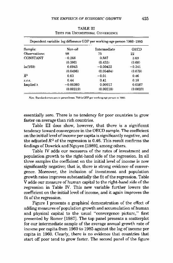
THE EMPIRICS OF ECONOMIC GROWTH 425
TABLE IIITESTS FOR UNCONDITIONAL CONVERGENCE
Dependent variable: log difference GDP per working-age person 1960-1985
Sample: Non-oil Intermediate OECDObservations: 98 75 22CONSTANT —0.266 0.587 3.69
(0.380) (0.433) (0.68)ln(Y60) 0.0943 —0.00423 —0.341
(0.0496) (0.05484) (0.079)7?2 0.03 —0.01 0.46s.e.e. 0.44 0.41 0.18Implied X —0.00360 0.00017 0.0167
(0.00219) (0.00218) (0.0023)
Note. Standard errors are in parentheses. Y60 is GDP per working-age person in 1960.
essentially zero. There is no tendency for poor countries to growfaster on average than rich countries.
Table III does show, however, that there is a significanttendency toward convergence in the OECD sample. The coefficienton the initial level of income per capita is significantly negative, andthe adjusted R 2 of the regression is 0.46. This result confirms thefindings of Dowrick and Nguyen [1989], among others.
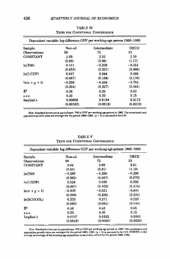
Table IV adds our measures of the rates of investment andpopulation growth to the right-hand side of the regression. In allthree samples the coefficient on the initial level of income is nowsignificantly negative; that is, there is strong evidence of conver-gence. Moreover, the inclusion of investment and populationgrowth rates improves substantially the fit of the regression. TableV adds our measure of human capital to the right-hand side of theregression in Table IV. This new variable further lowers thecoefficient on the initial level of income, and it again improves thefit of the regression.
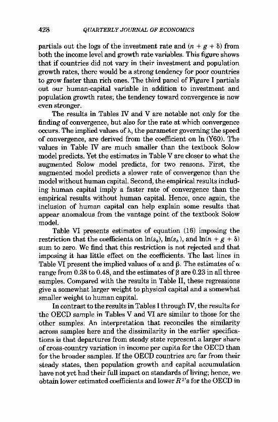
Figure I presents a graphical demonstration of the effect ofadding measures of population growth and accumulation of humanand physical capital to the usual "convergence picture," firstpresented by Romer [1987]. The top panel presents a scatterplotfor our intermediate sample of the average annual growth rate ofincome per capita from 1960 to 1985 against the log of income percapita in 1960. Clearly, there is no evidence that countries thatstart off poor tend to grow faster. The second panel of the figure
426 QUARTERLY JOURNAL OF ECONOMICS
TABLE IVTESTS FOR CONDITIONAL CONVERGENCE
Dependent variable: log difference GDP per working-age person 1960-1985
Sample: Non-oil Intermediate OECDObservations: 98 75 22
CONSTANT 1.93 2.23 2.19(0.83) (0.86) (1.17)
ln(Y60) -0.141 -0.228 -0.351(0.052) (0.057) (0.066)
ln(I/GDP) 0.647 0.644 0.392(0.087) (0.104) (0.176)
In(n + g + 3) -0.299 -0.464 -0.753(0.304) (0.307) (0.341)
172 0.38 0.35 0.62
s.e.e. 0.35 0.33 0.15
Implied A 0.00606 0.0104 0.0173(0.00182) (0.0019) (0.0019)
Note. Standard errors are in parentheses. Y60 is GDP per working-age person in 1960. The investment andpopulation growth rates are averages for the period 1960-1985. (g + 8) is assumed to be 0.05.
TABLE VTESTS FOR CONDITIONAL CONVERGENCE
Dependent variable: log difference GDP per working-age person 1960-1985
Sample: Non-oil Intermediate OECDObservations: 98 75 22
CONSTANT 3.04 3.69 2.81(0.83) (0.91) (1.19)
ln(Y60) -0.289 -0.366 -0.398(0.062) (0.067) (0.070)
ln(I/GDP) 0.524 0.538 0.335
(0.087) (0.102) (0.174)
In(n + g + 8) -0.505 -0.551 -0.844(0.288) (0.288) (0.334)
ln(SCHOOL) 0.233 0.271 0.223
(0.060) (0.081) (0.144)1:72 0.46 0.43 0.65
s.e.e. 0.33 0.30 0.15
Implied A 0.0137 0.0182 0.0203(0.0019) (0.0020) (0.0020)
Note. Standard errors are in parentheses. Y60 is GDP per working-age person in 1960. The investment andpopulation growth rates are averages for the period 1960-1985. (g + 1) is assumed to be 0.05. SCHOOL is theaverage percentage of the working-age population in secondary school for the period 1960-1985.

0
0 0 00
ooh°0 0 0 (Z0
(22O 0 00 0 0 o 80
(3% CSbO c99x)
o 6,5 7,5 8.5 9.5 10,5
Log output per working age adult:1960
U)co
O6
rn(0
4
ai 200
32 -2
55
U)co 6
0
rn• 4
a) 2
▪ 0
2
•
-2(9 55
B. Conditional on saving and population growth
6.5 7,5 8.5 9.5 10,5
THE EMPIRICS OF ECONOMIC GROWTH 427
A. Unconditional
Log output per working age adult:1960
C. Conditional on saving, population growth and human capitalLC)CO
6 6
• 4rn
• 20
_c 0
2 _25 5 6.5 7.5 8.5 9.5
10 5
Log output per working age adult:1960
FIGURE I
Unconditional versus Conditional Convergence
428 QUARTERLY JOURNAL OF ECONOMICS
partials out the logs of the investment rate and (n + g + 8) fromboth the income level and growth rate variables. This figure showsthat if countries did not vary in their investment and populationgrowth rates, there would be a strong tendency for poor countriesto grow faster than rich ones. The third panel of Figure I partialsout our human-capital variable in addition to investment andpopulation growth rates; the tendency toward convergence is noweven stronger.
The results in Tables W and V are notable not only for thefinding of convergence, but also for the rate at which convergenceoccurs. The implied values of X, the parameter governing the speedof convergence, are derived from the coefficient on In (Y60). Thevalues in Table IV are much smaller than the textbook Solowmodel predicts. Yet the estimates in Table V are closer to what theaugmented Solow model predicts, for two reasons. First, theaugmented model predicts a slower rate of convergence than themodel without human capital. Second, the empirical results includ-ing human capital imply a faster rate of convergence than theempirical results without human capital. Hence, once again, theinclusion of human capital can help explain some results thatappear anomalous from the vantage point of the textbook Solowmodel.
Table VI presents estimates of equation (16) imposing therestriction that the coefficients on ln(sk), ln(sk ), and ln(n + g + 8)sum to zero. We find that this restriction is not rejected and thatimposing it has little effect on the coefficients. The last lines inTable VI present the implied values of a and R. The estimates of arange from 0.38 to 0.48, and the estimates of p are 0.23 in all threesamples. Compared with the results in Table II, these regressionsgive a somewhat larger weight to physical capital and a somewhatsmaller weight to human capital.
In contrast to the results in Tables I through IV, the results forthe OECD sample in Tables V and VI are similar to those for theother samples. An interpretation that reconciles the similarityacross samples here and the dissimilarity in the earlier specifica-tions is that departures from steady state represent a larger shareof cross-country variation in income per capita for the OECD thanfor the broader samples. If the OECD countries are far from theirsteady states, then population growth and capital accumulationhave not yet had their full impact on standards of living; hence, weobtain lower estimated coefficients and lower R 2 's for the OECD in

THE EMPIRICS OF ECONOMIC GROWTH 429
TABLE VITESTS FOR CONDITIONAL CONVERGENCE, RESTRICTED REGRESSION
Dependent variable: log difference GDP per working-age person 1960-1985
Sample: Non-oil Intermediate OECDObservations: 98 75 22CONSTANT 2.46 3.09 3.55
(0.48) (0.53) (0.63)ln(Y60) -0.299 -0.372 -0.402
(0.061) (0.067) (0.069)ln(I/GDP) - In(n + g + 5) 0.500 0.506 0.396
(0.082) (0.095) (0.152)ln(SCHOOL) - ln(n + g + 5) 0.238 0.266 0.236
(0.060) (0.080) (0.141)R2 0.46 0.44 0.66s.e.e. 0.33 0.30 0.15Test of restriction:
p-value 0.40 0.42 0.47Implied X 0.0142 0.0186 0.0206
(0.0019) (0.0019) (0.0020)Implied a 0.48 0.44 0.38
(0.07) (0.07) (0.13)Implied 0 0.23 0.23 0.23
(0.05) (0.06) (0.11)
Note. Standard errors are in parentheses. Y60 is GDP per working-age person in 1960. The investment andpopulation growth rates are averages for the period 1960-1985. (g + 8) is assumed to be 0.05. SCHOOL is theaverage percentage of the working-age population in secondary school for the period 1960-1985.
specifications that do not consider out-of-steady-state dynamics.Similarly, the greater importance of departures from steady statefor the OECD would explain the finding of greater unconditionalconvergence. We find this interpretation plausible: World War IIsurely caused large departures from the steady state, and it surelyhad larger effects on the OECD than on the rest of the world. Witha value of X of 0.02, almost half of the departure from steady statein 1945 would have remained by the end of our sample in 1985.
Overall, our interpretation of the evidence on convergencecontrasts sharply with that of endogenous-growth advocates. Inparticular, we believe that the study of convergence does not showa failure of the Solow model. After controlling for those variablesthat the Solow model says determine the steady state, there issubstantial convergence in income per capita. Moreover, conver-gence occurs at approximately the rate that the model predicts.

430 QUARTERLY JOURNAL OF ECONOMICS
IV. INTEREST RATE DIFFERENTIALS AND CAPITAL MOVEMENTS
Recently, several economists, including Lucas [1988], Barro[1989], and King and Rebelo [1989], have emphasized an objectionto the Solow model in addition to those we have addressed so far:they argue that the model fails to explain either rate-of-returndifferences or international capital flows. In the models of SectionsI and II, the steady-state marginal product of capital, net ofdepreciation, is
(17) MPK — 8 = a(n + g + 8)Isk — 8.
Thus, the marginal product of capital varies positively with thepopulation growth rate and negatively with the saving rate.Because the cross-country differences in saving and populationgrowth rates are large, the differences in rates of return should alsobe large. For example, if a = 1/3, 8 = 0.03, and g = 0.02, then themean of the steady-state net marginal product is 0.12 in theintermediate sample, and the standard deviation is 0.08."
Two related facts seem inconsistent with these predictions.First, observed differentials in real interest rates appear smallerthan the predicted differences in the net marginal product ofcapital. Second, as Feldstein and Horioka [1980] first documented,countries with high saving rates have high rates of domesticinvestment rather than large current account surpluses: capitaldoes not flow from high-saving countries to low-saving countries.
Although these two facts indeed present puzzles to be resolved,it is premature to view them as a basis for rejecting the Solowmodel. The Solow model predicts that the marginal product ofcapital will be high in low-saving countries, but it does notnecessarily predict that real interest rates will also be high. Onecan infer the marginal product of capital from real interest rates onfinancial assets only if investors are optimizing and capital marketsare perfect. Both of these assumptions are questionable. It is
13. There is an alternative way of obtaining the marginal product of capital,which applies even outside of the steady state but requires an estimate of 8 and theassumption of no country-specific shifts to the production function. If one assumesthat the returns on human and physical capital are equalized within each country,then one can show that the MPK is proportional to y ('+ 13-1) / ( '+P ) . Therefore, for thetextbook Solow model in which a = 1/3 and 8 = 0, the MPK is inversely proportionalto the square of output. As King and Rebelo [1989] and others have noted, theimplied differences in rates of return across countries are incredibly large. Yet if a =8 = 1/3, then the MPK is inversely proportional to the square root of output. In thiscase, the implied cross-country differences in the MPK are much smaller and aresimilar to those obtained with equation (17).

THE EMPIRICS OF ECONOMIC GROWTH 431
possible that some of the most productive investments in poorcountries are in public capital, and that the behavior of thegovernments of poor countries is not socially optimal. In addition,it is possible that the marginal product of private capital is alsohigh in poor countries, yet those economic agents who could makethe productive investments do not do so because they face fi-nancing constraints or because they fear future expropriation.
Some evidence for this interpretation comes from examininginternational variation in the rate of profit. If capital earns itsmarginal product, then one can measure the marginal product ofcapital as
aMPK =
K/ Y .
That is, the return to capital equals capital's share in income (a)divided by the capital-output ratio (K/Y). The available evidenceindicates that capital's share is roughly constant across counties.Sachs [1979, Table 3] presents factor shares for the G-7 countries.His figures show that variation in these shares across countriesand over time is small." By contrast, capital-output ratios varysubstantially across countries: accumulating the investment datafrom Summers and Heston [1988] to produce estimates of thecapital stock, one finds that low-saving countries have capital-output ratios near one and high-saving countries have capital-output ratios near three. Thus, direct measurement of the profitrate suggests that there is large international variation in thereturn to capital.
The available evidence also indicates that expropriation risk isone reason that capital does not move to eliminate these differencesin the profit rate. Williams [1975] examines the experience offoreign investment in developing countries from 1956 to 1972. Hereports that, during this period, governments nationalized about19 percent of foreign capital, and that compensation averagedabout 41 percent of book value. It is hard to say precisely how muchof the observed differences in profit rates this expropriation riskcan explain. Yet, in view of this risk, it would be surprising if the
14. In particular, there is no evidence that rapid capital accumulation raisescapital's share Sachs [1979] reports that Japan's rapid accumulation in the 1960sand 1970s, for example, was associated with a rise in labor's share from 69 percentin 1962-1964 to 77 percent in 1975-1978. See also Atkinson [1975, p. 167].

432 QUARTERLY JOURNAL OF ECONOMICS
profit rates were not at least somewhat higher in developingcountries.
Further evidence on rates of return comes from the largeliterature on international differences in the return to education.Psacharopoulos [1985] summarizes the results of studies for over60 countries that analyze the determinants of labor earnings usingmicro data. Because forgone wages are the primary cost of educa-tion, the rate of return is roughly the percentage increase in thewage resulting from an additional year of schooling. He reportsthat the poorer the country, the larger the return to schooling.
Overall, the evidence on the return to capital appears consis-tent with the Solow model. Indeed, one might argue that itsupports the Solow model against the alternative of endogenous-growth models. Many endogenous-growth models assume constantreturns to scale in the reproducible factors of production; theytherefore imply that the rate of return should not vary with thelevel of development. Yet direct measurement of profit rates andreturns to schooling indicates that the rate of return is muchhigher in poor countries.
CONCLUSION
We have suggested that international differences in income percapita are best understood using an augmented Solow growthmodel. In this model output is produced from physical capital,human capital, and labor, and is used for investment in physicalcapital, investment in human capital, and consumption. Oneproduction function that is consistent with our empirical results isy = K1/31.1113 L113 .
This model of economic growth has several implications. First,the elasticity of income with respect to the stock of physical capitalis not substantially different from capital's share in income. Thisconclusion indicates, in contrast to Romer's suggestion, thatcapital receives approximately its social return. In other words,there are not substantial externalities to the accumulation ofphysical capital.
Second, despite the absence of externalities, the accumulationof physical capital has a larger impact on income per capita thanthe textbook Solow model implies. A higher saving rate leads tohigher income in steady state, which in turn leads to a higher levelof human capital, even if the rate of human-capital accumulation is

THE EMPIRICS OF ECONOMIC GROWTH 433
unchanged. Higher saving thus raises total factor productivity as itis usually measured. This difference between the textbook modeland the augmented model is quantitatively important. The text-book Solow model with a capital share of one third indicates thatthe elasticity of income with respect to the saving rate is one half.Our augmented Solow model indicates that this elasticity is one.
Third, population growth also has a larger impact on incomeper capita than the textbook model indicates. In the textbook modelhigher population growth lowers income because the availablecapital must be spread more thinly over the population of workers.In the augmented model human capital also must be spread morethinly, implying that higher population growth lowers measuredtotal factor productivity. Again, this effect is important quantita-tively. In the textbook model with a capital share of one third, theelasticity of income per capita with respect to n + g + 8 is — 1/2 . Inour augmented model this elasticity is —2.
Fourth, our model has implications for the dynamics of theeconomy when the economy is not in steady state. In contrast toendogenous-growth models, this model predicts that countrieswith similar technologies and rates of accumulation and populationgrowth should converge in income per capita. Yet this convergenceoccurs more slowly than the textbook Solow model suggests. Thetextbook Solow model implies that the economy reaches halfway tosteady state in about 17 years, whereas our augmented Solowmodel implies that the economy reaches halfway in about 35 years.
More generally, our results indicate that the Solow model isconsistent with the international evidence if one acknowledges theimportance of human as well as physical capital. The augmentedSolow model says that differences in saving, education, and popula-tion growth should explain cross-country differences in income percapita. Our examination of the data indicates that these threevariables do explain most of the international variation.
Future research should be directed at explaining why thevariables taken to be exogenous in the Solow model vary so muchfrom country to country. We expect that differences in tax policies,education policies, tastes for children, and political stability willend up among the ultimate determinants of cross-country differ-ences. We also expect that the Solow model will provide the bestframework for understanding how these determinants influence acountry's level of economic well-being.

434 QUARTERLY JOURNAL OF ECONOMICS
APPENDIX
Number Country
SampleGDP/adult
Growth1960-1985 I/Y SCHOOL
N I 0 1960 1985working
GDP age pop
1 Algeria 1 1 0 2485 4371 4.8 2.6 24.1 4.52 Angola 1 0 0 1588 1171 0.8 2.1 5.8 1.83 Benin 1 0 0 1116 1071 2.2 2.4 10.8 1.84 Botswana 1 1 0 959 3671 8.6 3.2 28.3 2.95 Burkina Faso 1 0 0 529 857 2.9 0.9 12.7 0.46 Burundi 1 0 0 755 663 1.2 1.7 5.1 0.47 Cameroon 1 1 0 889 2190 5.7 2.1 12.8 3.48 Central Mr. Rep. 1 0 0 838 789 1.5 1.7 10.5 1.49 Chad 1 0 0 908 462 -0.9 1.9 6.9 0.4
10 Congo, Peop. Rep. 1 0 0 1009 2624 6.2 2.4 28.8 3.811 Egypt 1 0 0 907 2160 6.0 2.5 16.3 7.012 Ethiopia 1 1 0 533 608 2.8 2.3 5.4 1.113 Gabon 0 0 0 1307 5350 7.0 1.4 22.1 2.614 Gambia, The 0 0 0 799 3.6 18.1 1.515 Ghana 1 0 0 1009 727 1.0 2.3 9.1 4.716 Guinea 0 0 0 746 869 2.2 1.6 10.917 Ivory Coast 1 1 0 1386 1704 5.1 4.3 12.4 2.318 Kenya 1 1 0 944 1329 4.8 3.4 17.4 2.419 Lesotho 0 0 0 431 1483 6.8 1.9 12.6 2.020 Liberia 1 0 0 863 944 3.3 3.0 21.5 2.521 Madagascar 1 1 0 1194 975 1.4 2.2 7.1 2.622 Malawi 1 1 0 455 823 4.8 2.4 13.2 0.623 Mali 1 1 0 737 710 2.1 2.2 7.3 1.024 Mauritania 1 0 0 777 1038 3.3 2.2 25.6 1.025 Mauritius 1 0 0 1973 2967 4.2 2.6 17.1 7.326 Morocco 1 1 0 1030 2348 5.8 2.5 8.3 3.627 Mozambique 1 0 0 1420 1035 1.4 2.7 6.1 0.728 Niger 1 0 0 539 841 4.4 2.6 10.3 0.529 Nigeria 1 1 0 1055 1186 2.8 2.4 12.0 2.330 Rwanda 1 0 0 460 696 4.5 2.8 7.9 0.431 Senegal 1 1 0 1392 1450 2.5 2.3 9.6 1.732 Sierra Leone 1 0 0 511 805 3.4 1.6 10.9 1.733 Somalia 1 0 0 901 657 1.8 3.1 13.8 1.134 S. Africa 1 1 0 4768 7064 3.9 2.3 21.6 3.035 Sudan 1 0 0 1254 1038 1.8 2.6 13.2 2.036 Swaziland 0 0 0 817 7.2 17.7 3.737 Tanzania 1 1 0 383 710 5.3 2.9 18.0 0.538 Togo 1 0 0 777 978 3.4 2.5 15.5 2.939 Tunisia 1 1 0 1623 3661 5.6 2.4 13.8 4.340 Uganda 1 0 0 601 667 3.5 3.1 4.1 1.141 Zaire 1 0 0 594 412 0.9 2.4 6.5 3.642 Zambia 1 1 0 1410 1217 2.1 2.7 31.7 2.443 Zimbabwe 1 1 0 1187 2107 5.1 2.8 21.1 4.4

THE EMPIRICS OF ECONOMIC GROWTH 435
APPENDIX
(CONTINUED)
Number Country
SampleGDP/adult
Growth1960-1985 I/Y SCHOOL
N I 0 1960 1985working
GDP age pop
44 Afghanistan 0 0 0 1224 1.6 6.9 0.945 Bahrain 0 0 0 30.0 12.146 Bangladesh 1 1 0 846 1221 4.0 2.6 6.8 3.247 Burma 1 1 0 517 1031 4.5 1.7 11.4 3.548 Hong Kong 1 1 0 3085 13,372 8.9 3.0 19.9 7.249 India 1 1 0 978 1339 3.6 2.4 16.8 5.150 Iran 0 0 0 3606 7400 6.3 3.4 18.4 6.551 Iraq 0 0 0 4916 5626 3.8 3.2 16.2 7.452 Israel 1 1 0 4802 10,450 5.9 2.8 28.5 9.553 Japan 1 1 1 3493 13,893 6.8 1.2 36.0 10.954 Jordan 1 1 0 2183 4312 5.4 2.7 17.6 10.855 Korea, Rep. of 1 1 0 1285 4775 7.9 2.7 22.3 10.256 Kuwait 0 0 0 77,881 25,635 2.4 6.8 9.5 9.657 Malaysia 1 1 0 2154 5788 7.1 3.2 23.2 7.358 Nepal 1 0 0 833 974 2.6 2.0 5.9 2.359 Oman 0 0 0 15,584 3.3 15.6 2.760 Pakistan 1 1 0 1077 2175 5.8 3.0 12.2 3.061 Philippines 1 1 0 1668 2430 4.5 3.0 14.9 10.662 Saudi Arabia 0 0 0 6731 11,057 6.1 4.1 12.8 3.163 Singapore 1 1 0 2793 14,678 9.2 2.6 32.2 9.064 Sri Lanka 1 1 0 1794 2482 3.7 2.4 14.8 8.365 Syrian Arab Rep. 1 1 0 2382 6042 6.7 3.0 15.9 8.866 Taiwan 0 0 0 8.0 20.767 Thailand 1 1 0 1308 3220 6.7 3.1 18.0 4.468 U. Arab Emirates 0 0 0 18,513 26.569 Yemen 0 0 0 1918 2.5 17.2 0.670 Austria 1 1 1 5939 13,327 3.6 0.4 23.4 8.071 Belgium 1 1 1 6789 14,290 3.5 0.5 23.4 9.372 Cyprus 0 0 0 2948 5.2 31.2 8.273 Denmark 1 1 1 8551 16,491 3.2 0.6 26.6 10.774 Finland 1 1 1 6527 13,779 3.7 0.7 36.9 11.575 France 1 1 1 7215 15,027 3.9 1.0 26.2 8.976 Germany, Fed. Rep. 1 1 1 7695 15,297 3.3 0.5 28.5 8.477 Greece 1 1 1 2257 6868 5.1 0.7 29.3 7.978 Iceland 0 0 0 8091 3.9 29.0 10.279 Ireland 1 1 1 4411 8675 3.8 1.1 25.9 11.480 Italy 1 1 1 4913 11,082 3.8 0.6 24.9 7.181 Luxembourg 0 0 0 9015 2.8 26.9 5.0
82 Malta 0 0 0 2293 6.0 30.9 7.1
83 Netherlands 1 1 1 7689 13,177 3.6 1.4 25.8 10.784 Norway 1 1 1 7938 19,723 4.3 0.7 29.1 10.0

436 QUARTERLY JOURNAL OF ECONOMICS
APPENDIX
(CONTINUED)
Number Country
SampleGDP/adult
Growth1960-1985 I/Y SCHOOL
N I 0 1960 1985working
GDP age pop
85 Portugal 1 1 1 2272 5827 4.4 0.6 22.5 5.886 Spain 1 1 1 3766 9903 4.9 1.0 17.7 8.087 Sweden 1 1 1 7802 15,237 3.1 0.4 24.5 7.988 Switzerland 1 1 1 10,308 15,881 2.5 0.8 29.7 4.889 Turkey 1 1 1 2274 4444 5.2 2.5 20.2 5.590 United Kingdom 1 1 1 7634 13,331 2.5 0.3 18.4 8.991 Barbados 0 0 0 3165 4.8 19.5 12.192 Canada 1 1 1 10,286 17,935 4.2 2.0 23.3 10.693 Costa Rica 1 1 0 3360 4492 4.7 3.5 14.7 7.094 Dominican Rep. 1 1 0 1939 3308 5.1 2.9 17.1 5.895 El Salvador 1 1 0 2042 1997 3.3 3.3 8.0 3.996 Guatemala 1 1 0 2481 3034 3.9 3.1 8.8 2.497 Haiti 1 1 0 1096 1237 1.8 1.3 7.1 1.998 Honduras 1 1 0 1430 1822 4.0 3.1 13.8 3.799 Jamaica 1 1 0 2726 3080 2.1 1.6 20.6 11.2
100 Mexico 1 1 0 4229 7380 5.5 3.3 19.5 6.6101 Nicaragua 1 1 0 3195 3978 4.1 3.3 14.5 5.8102 Panama 1 1 0 2423 5021 5.9 3.0 26.1 11.6103 Trinidad & Tobago 1 1 0 9253 11,285 2.7 1.9 20.4 8.8104 United States 1 1 1 12,362 18,988 3.2 1.5 21.1 11.9105 Argentina 1 1 0 4852 5533 2.1 1.5 25.3 5.0106 Bolivia 1 1 0 1618 2055 3.3 2.4 13.3 4.9107 Brazil 1 1 0 1842 5563 7.3 2.9 23.2 4.7108 Chile 1 1 0 5189 5533 2.6 2.3 29.7 7.7109 Colombia 1 1 0 2672 4405 5.0 3.0 18.0 6.1110 Ecuador 1 1 0 2198 4504 5.7 2.8 24.4 7.2111 Guyana 0 0 0 2761 1.1 32.4 11.7112 Paraguay 1 1 0 1951 3914 5.5 2.7 11.7 4.4113 Peru 1 1 0 3310 3775 3.5 2.9 12.0 8.0114 Surinam 0 0 0 3226 4.5 19.4 8.1115 Uruguay 1 1 0 5119 5495 0.9 0.6 11.8 7.0116 Venezuela 1 1 0 10,367 6336 1.9 3.8 11.4 7.0117 Australia 1 1 1 8440 13,409 3.8 2.0 31.5 9.8118 Fiji 0 0 0 3634 4.2 20.6 8.1119 Indonesia 1 1 0 879 2159 5.5 1.9 13.9 4.1120 New Zealand 1 1 1 9523 12,308 2.7 1.7 22.5 11.9121 Papua New Guinea 1 0 0 1781 2544 3.5 2.1 16.2 1.5
Note. Growth rates are in percent per year. I/Y is investment as a percentage of GDP, and SCHOOL is thepercentage of the working-age population in secondary school, both averaged for the period 1960-1985. N, I, and0 denote the non-oil, intermediate, and OECD samples.
THE EMPIRICS OF ECONOMIC GROWTH 437
HARVARD UNIVERSITY
UNIVERSITY OF CALIFORNIA AT BERKELEY
BROWN UNIVERSITY
REFERENCES
Atkinson, Anthony, The Economics of Inequality (Oxford: Clarendon Press, 1975).Azariadis, Costas, and Allan Drazen, "Threshold Externalities in Economic
Development," Quarterly Journal of Economics, CV (1990), 501-26.Barro, Robert J., "Economic Growth in a Cross Section of Countries," NBER
Working Paper 3120, September 1989.De Long, J. Bradford, "Productivity Growth, Convergence, and Welfare: Comment,"
American Economic Review, LXXVIII (1988), 1138-54.Dowrick, Steve, and Duc-Tho Nguyen, "OECD Comparative Economic Growth
1950-85: Catch-Up and Convergence," American Economic Review, LXXIX(1989), 1010-30.
Easterlin, Richard, "Why Isn't the Whole World Developed?" Journal of EconomicHistory, XLI (1981), 1-20.
Feldstein, Martin, and Charles Horioka, "Domestic Saving and InternationalCapital Flows," Economic Journal, XC (1980), 314-29.
Kendrick, John W., The Formation and Stocks of Total Capital (New York:Columbia University for NBER, 1976).
King, Robert G., and Sergio T. Rebelo, "Transitional Dynamics and EconomicGrowth in the Neoclassical Model," NBER Working Paper 3185, November1989.
Krueger, Anne 0., "Factor Endowments and per Capita Income Differences AmongCountries," Economic Journal, LXXVIII (1968), 641-59.
Lucas, Robert E. Jr., "On the Mechanics of Economic Development," Journal ofMonetary Economics, XXII (1988), 3-42.
Psacharopoulos, George, "Returns to Education: A Further International Updateand Implications," Journal of Human Resources, XX (1985), 583-604.
Rauch, James E., "The Question of International Convergence of per CapitaConsumption: An Euler Equation Approach," mimeo, August 1988, Universityof California at San Diego.
Romer, Paul, "Crazy Explanations for the Productivity Slowdown," NBER Macro-economics Annual, 1987,163-210.
"Capital Accumulation in the Theory of Long Run Growth," ModernBusiness Cycle Theory, Robert J. Barro, ed. (Cambridge, MA: Harvard Univer-sity Press, 1989a), pp. 51-127., "Human Capital and Growth: Theory and Evidence," NBER Working Paper3173, November 1989b.
Sachs, Jeffrey D., "Wages, Profit, and Macroeconomic Adjustment: A ComparativeStudy," Brookings Papers on Economic Activity (1979:2), 269-332.
Solow, Robert M., "A Contribution to the Theory of Economic Growth," QuarterlyJournal of Economics, LXX (1956), 65-94.
Summers, Robert, and Alan Heston, "A New Set of International Comparisons ofReal Product and Price Levels Estimates for 130 Countries, 1950-85," Reviewof Income and Wealth, XXXIV (1988), 1-26.
Williams, M. L., "The Extent and Significance of Nationalization of Foreign-ownedAssets in Developing Countries, 1956-1972," Oxford Economic Papers, XXVII(1975), 260-73.