null space of the stoichiometrix matrix - helsinki

Null space of the stoichiometrix matrix

I Any flux vector v that the cell can maintain in a steady-stateis a solution to the homogeneous system of equations

Sv = 0

I By definition, the set

N (S) = {u|Su = 0}

contains all valid flux vectors

I In linear algebra N (A) is referred to as the null space of thematrix A

I Studying the null space of the stoichiometric matrix can giveus important information about the cell’s capabilities

Null space of the stoichiometric matrix

The null space N (S) is a linear vector space, so all properties oflinear vector spcaes follow, e.g:

I N (S) contains the zero vector, and closed under linearcombination: v1, v2 ∈ N (S) =⇒ α1v1 + αv2 ∈ N (S)

I The null space has a basis {k1, . . . , kq}, a set of q ≤ min(n, r)linearly independent vectors, where r is the number ofreactions and n is the number of metabolites.

I The choice of basis is not unique, but the number q of vectorit contains is determined by the rank of S .

Null space and feasible steady state rate vectors

I The kernel K = (k1, . . . , kq) of the stoichiometric matrixformed by the above basis vectors has a row corresponding toeach reaction. (Note: the term ’kernel’ here has no relation tokernel methods and SVMs)

I K characterizes the feasible steady state reaction rate vectors:for each feasible flux vector v, there is a vector b ∈ Rq suchthat Kb = v

I In other words, any steady state flux vector is a linearcombination

b1k1 + · · ·+ bqkq

of the basis vectors of N (S).

Applications of null space analysis

Three properties of the metabolic network can be found directlyfrom the kernel matrix

I Dead ends in metabolism (reactions that cannot carry a flus inany steady state): correspond to identically zero rows in thekernel

I Enzyme subsets (reactions that are forced to operate in lockstep in any steedy state): correspond to kernel rows that arescalar multiples of each other

I Independent components (groups of reactions that can carryflux independently from reactions outside the group):block-diagonal structure in the kernel

Singular value decomposition of S

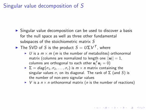
I Singular value decomposition can be used to discover a basisfor the null space as well as three other fundamentalsubspaces of the stoichiometric matrix S

I The SVD of S is the product S = UΣV T , whereI U is a m ×m (m is the number of metabolites) orthonormal

matrix (columns are normalized to length one ||u|| = 1,columns are orthogonal to each other uT

i uj = 0)I Σ = diag(σ1, σ2, . . . , σr ) is m × n matrix containing the

singular values σi on its diagonal. The rank of Σ (and S) isthe number of non-zero signular values

I V is a n× n orthonormal matrix (n is the number of reactions)

Singular value decomposition of S : matrix U

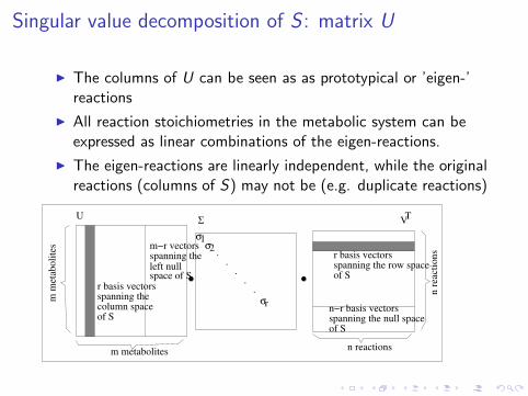
I The columns of U can be seen as as prototypical or ’eigen-’reactions

I All reaction stoichiometries in the metabolic system can beexpressed as linear combinations of the eigen-reactions.

I The eigen-reactions are linearly independent, while the originalreactions (columns of S) may not be (e.g. duplicate reactions)

TV

n reactions

spanning the row space of S

r basis vectors

spanning the null space of S

n−r basis vectors

n r

eact

ion

s

m metabolites

σ1σ2

σspanning ther basis vectors

column spaceof S

UΣ

m m

etab

oli

tes m−r vectorsspanning theleft nullspace of S

r

..

..

.


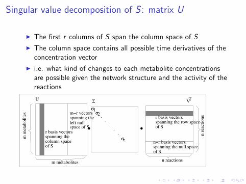
I The first r columns of S span the column space of S

I The column space contains all possible time derivatives of theconcentration vector

I i.e. what kind of changes to each metabolite concentrationsare possible given the network structure and the activity of thereactions

TV

n reactions


r basis vectors


n−r basis vectors

n r

eact

ion

s

m metabolites

σ1σ2


column spaceof S

UΣ

m m

etab

oli


r

..

..

.


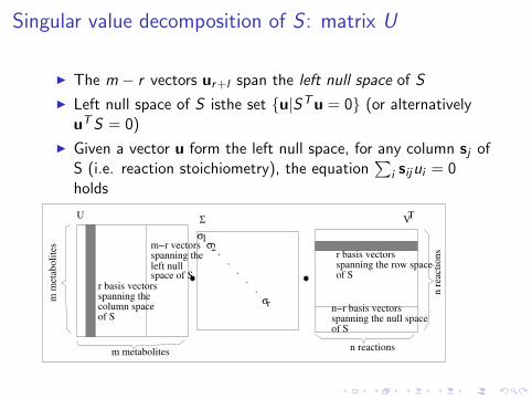
I The m − r vectors ur+l span the left null space of S

I Left null space of S isthe set {u|STu = 0} (or alternativelyuTS = 0)

I Given a vector u form the left null space, for any column sj ofS (i.e. reaction stoichiometry), the equation

∑i sijui = 0

holds

TV

n reactions


r basis vectors


n−r basis vectors

n r

eact

ion

s

m metabolites

σ1σ2


column spaceof S

UΣ

m m

etab

oli


r

..

..

.


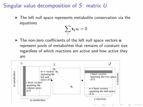
I The left null space represents metabolite conservation via theequations ∑

i

sijui = 0

I The non-zero coefficients of the left null space vectors urepresent pools of metabolites that remains of constant sizeregardless of which reactions are active and how active theyare

TV

n reactions


r basis vectors


n−r basis vectors

n r

eact

ion

s

m metabolites

σ1σ2


column spaceof S

UΣ

m m

etab

oli

tes m−r vectors

spanning theleft nullspace of S

r

..

..

.

Conservation in PPP

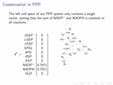
The left null space of our PPP system only contains a singlevector, stating that the sum of NADP+ and NADPH is constant inall reactions.

lT =

βG6PαG6PβF6P6PGL6PGR5PX5P

NADP+

NADPHH2O

0000000

0.70710.7071

0

R1

R2

R3

R4

R5

R6

R7

R8

R9

R10

R11

G6P

F6PG6P

6PGL

6PGR5P

X5P

H O2

α

ββ

NADPH

NADP

Singular value decomposition of S : matrix V

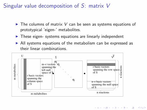
I The columns of matrix V can be seen as systems equations ofprototypical ’eigen-’ metabolites.

I These eigen- systems equations are linearly independent

I All systems equations of the metabolism can be expressed astheir linear combinations.

TV

n reactions


r basis vectors


n−r basis vectors

n r

eact

ion

s

m metabolites

σ1σ2


column spaceof S

UΣ

m m

etab

oli

tes m−r vectors


r

..

..

.


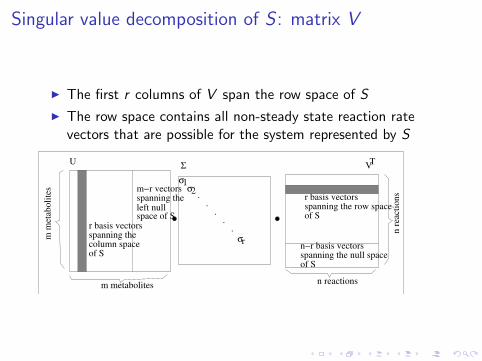
I The first r columns of V span the row space of S

I The row space contains all non-steady state reaction ratevectors that are possible for the system represented by S

TV

n reactions


r basis vectors


n−r basis vectors

n r

eact

ion

s

m metabolites

σ1σ2


column spaceof S

UΣ

m m

etab

oli

tes m−r vectors


r

..

..

.


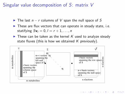
I The last n − r columns of V span the null space of S

I These are flux vectors that can operate in steady state, i.e.statifying Svl = 0, l = r + 1, . . . , n

I These can be taken as the kernel K used to analyze steadystate fluxes (this is how we obtained K previously).

TV

n reactions


r basis vectors


n−r basis vectors

n r

eact

ion

s

m metabolites

σ1σ2


column spaceof S

UΣ

m m

etab

oli

tes m−r vectors


r

..

..

.

SVD of PPP

MATLAB script pppsvd .m computes

I The stoichiometric matrix S

I The singular value decomposition S = UΣV T

I The kernel matrix of the null space K

I The kernel matrix of the left null space Kleft

Other conserved quantitites

I Above look at conservation of pool sizes of metabolitesI Conservation of other items can be analyzed as well:

I Elemental balance: for each element species (C,N,O,P,...) thenumber of elements is conserved

I Charge balance: total electrical charge, the total number ofelectrons in a reaction does not change.

Elemental balancing (1/2)

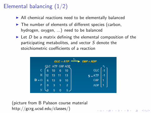
I All chemical reactions need to be elementally balanced

I The number of elements of different species (carbon,hydrogen, oxygen, ...) need to be balanced

I Let D be a matrix defining the elemental composition of theparticipating metabolites, and vector S denote thestoichiometric coefficients of a reaction

(picture from B Palsson course materialhttp://gcrg.ucsd.edu/classes/)

Elemental balancing (2/2)

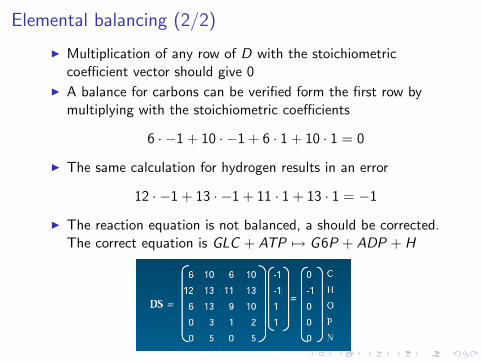
I Multiplication of any row of D with the stoichiometriccoefficient vector should give 0

I A balance for carbons can be verified form the first row bymultiplying with the stoichiometric coefficients

6 · −1 + 10 · −1 + 6 · 1 + 10 · 1 = 0

I The same calculation for hydrogen results in an error

12 · −1 + 13 · −1 + 11 · 1 + 13 · 1 = −1

I The reaction equation is not balanced, a should be corrected.The correct equation is GLC + ATP 7→ G6P + ADP + H

Basis steady state flux modes from SVD

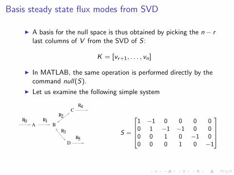
I A basis for the null space is thus obtained by picking the n− rlast columns of V from the SVD of S :

K = [vr+1, . . . , vn]

I In MATLAB, the same operation is performed directly by thecommand null(S).

I Let us examine the following simple system

R2

R3

R1R0

R4

R5

B

C

A

D

S =

1 −1 0 0 0 00 1 −1 −1 0 00 0 1 0 −1 00 0 0 1 0 −1


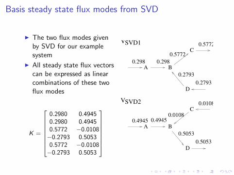
I The two flux modes givenby SVD for our examplesystem

I All steady state flux vectorscan be expressed as linearcombinations of these twoflux modes

K =

0.2980 0.49450.2980 0.49450.5772 −0.0108−0.2793 0.50530.5772 −0.0108−0.2793 0.5053

0.4945

0.0108

0.0108

0.5053

0.5053

0.298 0.298

0.5772

0.5772

0.2793

0.2793

B

C

A

D

VSVD2

0.4945

B

C

A

D

VSVD1


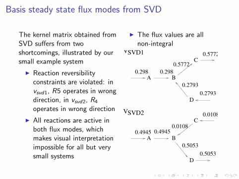
The kernel matrix obtained fromSVD suffers from twoshortcomings, illustrated by oursmall example system

I Reaction reversibilityconstraints are violated: invsvd1, R5 operates in wrongdirection, in vsvd2, R4

operates in wrong direction

I All reactions are active inboth flux modes, whichmakes visual interpretationimpossible for all but verysmall systems

I The flux values are allnon-integral

0.4945

0.0108

0.0108

0.5053

0.5053

0.298 0.298

0.5772

0.5772

0.2793

0.2793

B

C

A

D

VSVD2

0.4945

B

C

A

D

VSVD1

Choice of basis

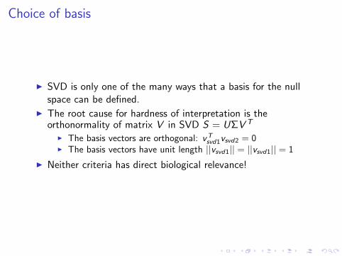
I SVD is only one of the many ways that a basis for the nullspace can be defined.

I The root cause for hardness of interpretation is theorthonormality of matrix V in SVD S = UΣV T

I The basis vectors are orthogonal: vTsvd1vsvd2 = 0

I The basis vectors have unit length ||vsvd1|| = ||vsvd1|| = 1

I Neither criteria has direct biological relevance!

Biologically meaningful pathways

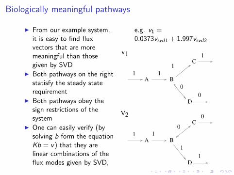
I From our example system,it is easy to find fluxvectors that are moremeaningful than thosegiven by SVD

I Both pathways on the rightstatisfy the steady staterequirement

I Both pathways obey thesign restrictions of thesystem

I One can easily verify (bysolving b form the equationKb = v) that they arelinear combinations of theflux modes given by SVD,

e.g. v1 =0.0373vsvd1 + 1.997vsvd2

1 1

1

1

0

0

1

0

0

1

1

B

C

A

D

V

B

C

A

D

V1

1

2

Elementary flux modes

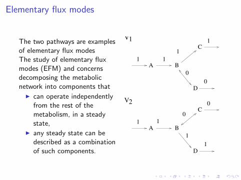
The two pathways are examplesof elementary flux modesThe study of elementary fluxmodes (EFM) and concernsdecomposing the metabolicnetwork into components that

I can operate independentlyfrom the rest of themetabolism, in a steadystate,

I any steady state can bedescribed as a combinationof such components.

1 1

1

1

0

0

1

0

0

1

1

B

C

A

D

V

B

C

A

D

V1

1

2

Representing EFMs

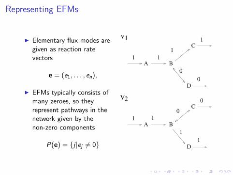
I Elementary flux modes aregiven as reaction ratevectors

e = (e1, . . . , en),

I EFMs typically consists ofmany zeroes, so theyrepresent pathways in thenetwork given by thenon-zero components

P(e) = {j |ej 6= 0}

1 1

1

1

0

0

1

0

0

1

1

B

C

A

D

V

B

C

A

D

V1

1

2

Properties of elementary flux modes

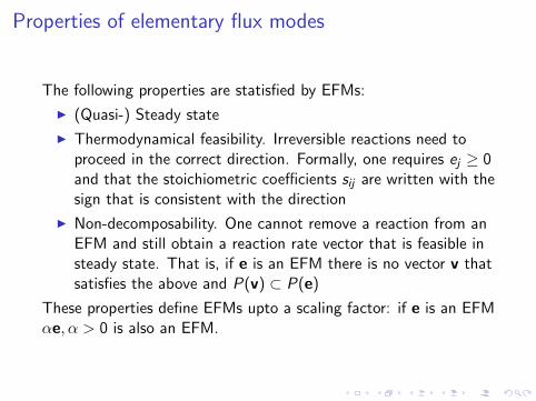
The following properties are statisfied by EFMs:

I (Quasi-) Steady state

I Thermodynamical feasibility. Irreversible reactions need toproceed in the correct direction. Formally, one requires ej ≥ 0and that the stoichiometric coefficients sij are written with thesign that is consistent with the direction

I Non-decomposability. One cannot remove a reaction from anEFM and still obtain a reaction rate vector that is feasible insteady state. That is, if e is an EFM there is no vector v thatsatisfies the above and P(v) ⊂ P(e)

These properties define EFMs upto a scaling factor: if e is an EFMαe, α > 0 is also an EFM.

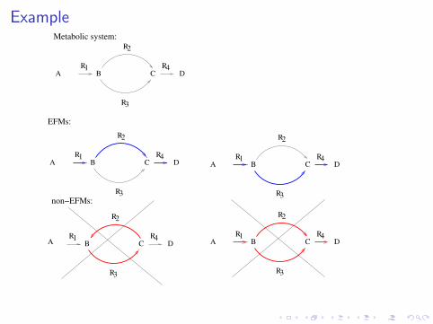
Example

R4

R2

R3

R1

R4

R2

R3

R1R4

R2

R3

R1

R4

R2

R3

R1A DB C

R4

R2

R3

R1A DB

A DB A DB C

C

C

Metabolic system:

A DB C

EFMs:

non−EFMs:

EFMs and steady state fluxes

I Any steady state flux vector v can be represented as anon-negative combination of the elementary flux modes:v =

∑j αjej , where αj ≥ 0.

I However, the representation is not unique: one can often findseveral coefficient sets α that satisfy the above.

I Thus, a direct composition of a flux vector into the underlyingEFPs is typically not possible. However, the spectrum ofpotential contributions can be analysed

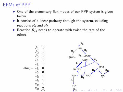
EFMs of PPPI One of the elementary flux modes of our PPP system is given

belowI It consist of a linear pathway through the system, exluding

reactions R6 and R7

I Reaction R11 needs to operate with twice the rate of theothers

efm1 =

R1

R2

R3

R4

R5

R6

R7

R8

R9

R10

R11

11111001112

R1

R2

R3

R4

R8

R9

R10

R11

R5R

6

R7

G6P

F6PG6P

6PGL

6PGR5P

X5P

H O2

α

ββ

NADPH

NADP

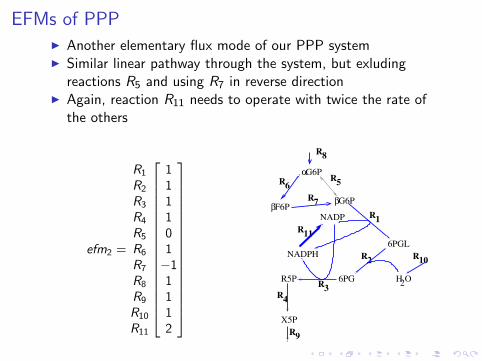
EFMs of PPPI Another elementary flux mode of our PPP systemI Similar linear pathway through the system, but exluding

reactions R5 and using R7 in reverse directionI Again, reaction R11 needs to operate with twice the rate of

the others

efm2 =

R1

R2

R3

R4

R5

R6

R7

R8

R9

R10

R11

111101−11112

R1

R2

R3

R4

R5

R8

R9

R10

R11

R6

R7

G6P

F6PG6P

6PGL

6PGR5P

X5P

H O2

α

ββ

NADPH

NADP

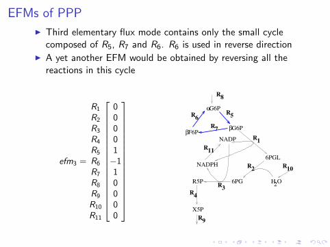
EFMs of PPP

I Third elementary flux mode contains only the small cyclecomposed of R5, R7 and R6. R6 is used in reverse direction

I A yet another EFM would be obtained by reversing all thereactions in this cycle

efm3 =

R1

R2

R3

R4

R5

R6

R7

R8

R9

R10

R11

00001−110000

R1

R2

R3

R4

R5

R8

R9

R10

R11

R6

R7

G6P

F6PG6P

6PGL

6PGR5P

X5P

H O2

α

ββ

NADPH

NADP

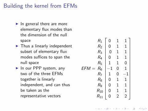
Building the kernel from EFMs

I In general there are moreelementary flux modes thanthe dimension of the nullspace

I Thus a linearly independentsubset of elementary fluxmodes suffices to span thenull space

I In our PPP system, anytwo of the three EFMstogether is linearlyindependent, and can thusbe taken as therepresentative vectors

EFM =

R1

R2

R3

R4

R5

R6

R7

R8

R9

R10

R11

0 1 10 1 10 1 10 1 11 1 0−1 0 11 0 −10 1 10 1 10 1 10 2 2

Software for finding EFMs

I From small systems it is relatively easy to find the EFMs bymanual inspection

I For larger systems this becomes impossible, as the number ofEFMs grows easily very large

I Computational methods have been devised for finding theEFMs by Heinrich & Schuster, 1994 and Urbanczik andWagner, 2005

I Implemented in MetaTool package

Extreme pathways

I Extreme pathways (EP) are an alternative formalism to EFMsfor analyzing the steady state flux space

I Extreme pathways differ from EFMs in two waysI The EPs are always non-negative v ≥ 0. Bi-directional

reactions need to be represented as separate forward andbackward reactions.

I In EPs the maximum rates of the reactions are also considered0 ≤ vi ≤ vi,max

Extreme pathways

I All steady state flux vectors can be expressed as convexcombinations of extreme pathways pi : v =

∑i αipi , 0 ≤ αi

I Geometrically, the extreme pathways form a high-dimensionalpolyhedron enclosing all legal steady state fluxes

I Flux balance analysis uses this polyhedron as the feasible setof fluxes where the flux vector optimizing the objective (e.g.biomass growth) needs to reside

null space of the stoichiometrix matrix - helsinki

Documents