number theory and combinatorics - ias.ac.in · preface over the last two decades, my expositions in...
TRANSCRIPT

Number Theory
and
Combinatorics
B SURY
Stat-Math Unit, Indian Statistical Institute, Bengaluru, India.

All rights reserved. No part of this publication may be reproduced, storedin a retrieval system or transmitted, in any form or by any means,electronic, mechanical, photocopying, recording, or otherwise, withoutprior permission of the publisher.
c© Indian Academy of Sciences 2017Reproduced from Resonance–journal of science educationReformatted by TNQ Books and Journals Pvt Ltd, www.tnq.co.inPublished by Indian Academy of Sciences

Foreword
The Masterclass series of eBooks brings together pedagogical articles onsingle broad topics taken from Resonance, the Journal of Science Educa-tion, that has been published monthly by the Indian Academy of Sciencessince January 1996. Primarily directed at students and teachers at the un-dergraduate level, the journal has brought out a wide spectrum of articlesin a range of scientific disciplines. Articles in the journal are written in astyle that makes them accessible to readers from diverse backgrounds, andin addition, they provide a useful source of instruction that is not alwaysavailable in textbooks.
The third book in the series, ‘Number Theory and Combinatorics’, is byProf. B Sury. A celebrated mathematician, Prof. Sury’s career has largelybeen at the Tata Institute of Fundamental Research, Mumbai’, and theIndian Statistical Institute, Bengaluru, where he is presently professor. Hehas contributed pedagogical articles regularly to Resonance, and his arti-cles on Number Theory and Combinatorics comprise the present book. Hehas also served for many years on the editorial board of Resonance.
Prof. Sury has contributed significantly to research in the areas of linear al-gebraic groups over global and local fields, Diophantine equations, divisionalgebras, central extensions of p-adic groups, applications of density theo-rems in number theory, K-theory of Chevalley groups, combinatorial num-ber theory, and generation of matrix groups over rings. The book, whichwill be available in digital format, and will be housed as always on theAcademy website, will be valuable to both students and experts as a usefulhandbook on Number Theory and Combinatorics.
Amitabh JoshiEditor of Publications
Indian Academy of SciencesAugust 2017
iii


About the Author
B Sury is a Professor of Mathematics at the Indian Statistical Institute inBangalore since 1999. He was earlier at the Tata Institute of FundamentalResearch, Mumbai, where he also got his PhD. Sury’s professional interestshave been very diverse: from the theory of algebraic groups and arithmeticgroups, to algebraic K-theory, and number theory. He has contributed tothese areas both through research papers and also through books.
Sury enjoys thinking about mathematical problems at all levels, and hastaken keen interest in promoting problem solving skills. As a result of hisabilities and willingness to shoulder responsibilities both in training stu-dents, and in writing exposition for students, he is universally sought afterfor any student activity in the country: he has been associated with sev-eral student magazines in the country, perhaps the important of them all,‘Resonance’ for the last two decades, as well the Ramanujan Math Soci-eties Newsletter. He has been an important member of the MathematicalOlympiad Program of the country. Sury is known to friends and colleaguesfor his wit and humor, which seems to come almost instantaneously; onecan enjoy some of his limericks on his webpage at ISI. The present volumebrings together some of the writings of B Sury on Number Theory andCombinatorics which have appeared in ‘Resonance’ during the last twodecades. Each of the articles is a masterpiece! I am sure it will be a feastfor the intellect of any reader with some mathematical inclination.
Dipendra PrasadTIFR, Mumbai
v


Contents
1 Cyclotomy and Cyclotomic Polynomials: The Story of how GaussNarrowly Missed Becoming a Philologist
1
2 Polynomials with Integer Values 25
3 How Far Apart are Primes? Bertrand’s Postulate 37
4 Sums of Powers, Bernoulli and the Riemann Zeta function 47
5 Frobenius and His Density Theorem for Primes 55
6 When is a Decimal Expansion Irrational? 63
7 Revisiting Kummer’s and Legendre’s Formulae 65
8 Bessels Contain Continued Fractions of Progressions 69
9 The Prime Ordeal 75
10 Extending Given Digits to Make Primes or Perfect Powers 87
11 An Irrational Walk and Why 1 is Not Congruent 93
12 Covering the Integers 99
13 S Chowla and S S Pillai: The Story of Two Peerless IndianMathematicians
103
14 Multi-variable Chinese Remainder Theorem 127
15 Which Positive Integers are Interesting? 135
16 Counting, Recounting and Matching 149
17 Odd if it isn’t an Even Fit! Lighting up Tiling 161
18 Polya’s One Theorem with 100 pages of Applications 169
vii


Preface
Over the last two decades, my expositions in Resonance are on roughlytwo topics – (i) number theory and combinatorics, and (ii) group theory. Inthis volume, some of the expositions related to the former topic have beenput together. The chapter on the work of Chowla and Pillai is part of anarticle written in collaboration with R Thangadurai that appeared in Reso-nance. I would like to thank Thangadurai for allowing me to include it here.I have attempted to retain the original write-ups of the articles as much aspossible other than carrying out some corrections and (minor) additions.As this is a compendium of articles that appeared in Resonance, at timessome material is repeated in different chapters. Further, this makes thecompilation somewhat uneven in terms of levels of mathematical maturityrequired of the reader despite my efforts to ensure uniformity.
Concerning my philosophy of mathematics dissemination, I havestaunchly held the opinion that many topics in mathematics which aresupposedly advanced in nature, can be exposed in a manner understand-able to a motivated undergraduate or postgraduate student. It may besomewhat of a challenge to make it comprehensible while still retaining theessential depth and technicality of the content, but it should neverthelessbe possible. Over the years, I have tried to put this in practice. One of thebest compliments I have received from Professor K R Parthasarathy, whotold a visitor that he had learnt some number theory through these articles.Despite this obvious exaggeration (or rather because of this perhaps!), I wasencouraged to keep trying to share some of the beautiful number theoreticand combinatorial ideas I myself enjoyed learning. To my surprise, I haveoccasionally found references to some of these articles in university coursesin various places, and that has been fulfilling. The years 1981-1999 at theTata Institute of Fundamental Research – where I first saw what excellencemeans – have had a positive effect on me in terms of being able to appreci-ate good mathematics (irrespective of whether I could originally contributeto it or not). During those years, it was a lot of fun to learn over conversa-tions near the sea-side, at the coffee-table, and during ping-pong sessionsfrom Madhav Nori, Venkataramana, Dipendra Prasad, C S Rajan, RaviRao, Raja Sridharan, Amit Roy, R R Simha, Bhatwadekar, Subramaniam,Parameswaran, Nitin Nitsure, Kapil Paranjape, Stephen Lobo, Kumare-san, and many others. In most instances, I would excitedly come up tothem with something I had “seen”, and they would be willing listeners andteachers. In later years, I have always benefited by talking to students andrealizing time and again what they found simultaneously enjoyable as well
ix
as not easy to understand. In almost all cases, after a meeting or discussionwith some students, I felt compelled to write on a certain topic. Inciden-tally, some of the summer projects that students worked on have appearedin Resonance as well and, many of them were rewritten by me – showingmy desire to communicate in a particular way. I personally know severalcolleagues who are much better at writing such expositions but, not manyof them seem to find the time to write at this level. I wish they would.
Finally, I am indebted to Professor Ram Ramaswamy for suggesting thepublication of this volume, for convincing me that it could be useful, andfor pushing me to finish this process.
B SuryJuly 2017
x

Cyclotomy and Cyclotomic Polynomials:The Story of how Gauss NarrowlyMissed Becoming a Philologist
A person who does arousemuch admiration and a million wows!Such a mathematicians’ princehas not been born since.I talk of Carl Friedrich Gauss!
Cyclotomy – literally ‘circle-cutting’ – was a puzzle begun more than2000 years ago by the Greek geometers. In this pastime, they used twoimplements – a ruler to draw straight lines and a pair of compasses to drawcircles. The problem of cyclotomy was to divide the circumference of a circleinto n equal parts using only these two implements.
As these n points on the circle are also the corners of a regular n-gon,the problem of cyclotomy is equivalent to the problem of constructing theregular n-gon using only a ruler and a pair of compasses. Euclid’s schoolconstructed the equilateral triangle, the square, the regular pentagon andthe regular hexagon. For more than 2000 years mathematicians had beenunanimous in their view that for no prime p bigger than 5 can the p-gonbe constructed by ruler and compasses. The teenager Carl Friedrich Gaussproved a month before he was 19 that the regular 17-gon is constructible.He did not stop there but went ahead to completely characterise all thosen for which the regular n-gon is constructible! This achievement of Gaussis one of the most surprising discoveries in mathematics. This feat wasresponsible for Gauss dedicating his life to the study of mathematics insteadof philology1 in which too he was equally proficient.
In his mathematical diary2 maintained from 1796 to 1814, he made hisfirst entry on the 30th of March and announced the construction of theregular 17-gon. It is said that he was so proud of this discovery that herequested that the regular 17-gon be engraved on his tombstone! This wishwas, however, not carried out.
An amusing story alludes to Kastner, one of his teachers at the universityof Gottingen, and an amateur poet. When Gauss told him of his discovery,Kastner was skeptical and did not take him seriously. Gauss insisted that
The chapter is a modified version of an article that first appeared in Resonance, Vol. 4, No. 12,
pp. 41–53, December 1999.1By 18, Gauss was already an expert in Greek, Latin, French and German. At the age of 62, he
took up the study of Russian and read Pushkin in the original.2The diary was found only in 1898!
1
Cyclotomy and Cyclotomic Polynomials
he could prove his result by reducing to smaller degree equations and,being fond of calculations, also showed the co-ordinates of the 17 pointscomputed to several decimal places. Kastner is said to have claimed thathe already knew such approximations long before. In retaliation, some timelater, Gauss described Kastner as the best poet among mathematicians andthe best mathematician among poets!
Gauss’s proof was not only instrumental in making up his mind to take upmathematics as a career but it is also the first instance when a mathematicalproblem from one domain was rephrased in another domain and solvedsuccessfully. In this instance, the geometrical problem of cyclotomy wasreset in algebraic terms and solved. So, let us see more in detail whatcyclotomy is all about.
The unit circle is given to us3 and we would like to divide it into n equalparts using only the ruler and compasses. It should be noted that the rulercan be used only to draw a line joining two given points and not for measuringlengths. For this reason, one sometimes uses the word straightedge instead ofa ruler.
If we view the plane as the complex plane, the unit circle has the equationz = eiθ. Since arc length is proportional to the angle subtended, the n com-plex numbers e2πik/n, 1 ≤ k ≤ n cut the circumference into n equal parts.
As we might fix a diameter to be on the x-axis, the problem may also bevariously posed as the problem of using only the ruler and the compasses to:
(i) find the roots of zn = 1, or(ii) construct the angle 2π/n.
Since, by coordinate geometry, a line and a circle have equations, respec-tively, of the form ax+ by = c and (x− s)2 + (y − t)2 = r2, their points ofintersection (if any) are the common roots. Eliminating one of x, y leads to aquadratic equation for the other. Therefore, the use of ruler and compassesamounts in algebraic terms to solving a chain of quadratic equations.
Before we go further, we need to clarify one point. On the one hand, weseem to be talking of constructing lengths and, on the other hand, we seemto want to mark off certain specific points on the plane corresponding tothe vertices of a regular n-gon. To remove any confusion due to this, let usexplain how these are equivalent.
1. Some Easy Constructions Possible with a Ruler and a Pairof Compasses
1. Drop a perpendicular on a given line l from a point P outside it(Figure 1).
3It is understood that the centre is also given.
2

Cyclotomy and Cyclotomic Polynomials
P
A
Q
B
l
Draw a circle centred at P cutting l at A and B. Draw circles centred atA and B having radii AP and BP , respectively. The latter circles intersectat P and Q and PQ is perpendicular to l.
2. Draw a perpendicular to a given line l through a point P on it(Figure 2).
C
B
D
A
P l
Draw any circle centred at P intersecting l at A and B. Then, the circlescentred at A and B with the common radius AB intersect at two points Cand D. Then, CD passes through P and is perpendicular to l.
3. Draw a line parallel to a given line through a point outside.This follows by doing the above constructions in succession.
4. Bisect a given segment AB.This is obvious from Figure 2. The circles centred at A and B having
the common radius AB intersect at two points. The line joining these twopoints is the perpendicular bisector.
Marking the point (a, b) on the plane is, by these observations, equivalentto the construction of the lengths |a| and |b|. Further, one can view the sameas the construction of the complex number a+ ib.
5. If a and b are constructed real numbers, then the roots of the polynomialx2 − ax+ b = 0 are constructible as well.
Actually, in the discussion of cyclotomy, we will need to deal only withthe case when the roots of such a quadratic equation are real. In this case(Figure 3), draw the circle with the segment joining the points (0, 1) and(a, b) as its diameter. The points of intersection of this circle with tile x-axis
are the roots a±√a2−4b2 of the given quadratic equation x2 − ax+ b = 0.
3

Cyclotomy and Cyclotomic Polynomials
Even when the roots of x2 − ax + b = 0 are not real, they can be con-
structed easily. In this case, we need to construct the points (a2 ,±√
4b−a22 ).
But, as we
x-axis
(0,1)
(0,0)
(a,b)y-axis
( ,0)a+√a2–4b2( ,0)a–√a2–4b
2
observed earlier, we can drop perpendiculars and it suffices to construct theabsolute value of these roots which is
√b. This is accomplished by drawing
the circle with the segment joining (0, 1) and (0,−b) as diameter and notingthat it meets the x-axis at the points (±
√b, 0).
With this renewed knowledge, let us return to cyclotomy.For n = 2, one needs to draw a diameter and this is evidently achieved
by the ruler.For n = 3, the equation z3 − 1 = 0 reduces to the equations z − l = 0 or
z2 + z + l = O. The roots of the latter are −1±i√
32 . So, we have to bisect
the segment [−1, 0] and the points of intersection of this bisector with theunit circle are the points we want to mark off on the circle.
For n = 4, again only bisection (of the x-axis) is involved. This alreadydemonstrates clearly that if the regular n-gon can be constructed, then socan the 2rn-gon be for any r. In particular, the 2r-gons are constructible.
To construct the regular pentagon, one has to construct the roots of z5−1= 0. These are the 5-th roots of unity ζk; i ≤ k ≤ 5 where ζ = e2iπ/5. Nowthe sum of the roots of z5 − 1 = 0 is
0 = ζ + ζ2 + ζ3 + ζ4 + ζ5.
On using this and the fact that ζ5 = 1, we get
(ζ2 + ζ3)(ζ + ζ4) = ζ + ζ2 + ζ3 + ζ4 = −1.
On the other hand, we also have their sum
(ζ2 + ζ3) + (ζ + ζ4) = −1.
4
Cyclotomy and Cyclotomic Polynomials
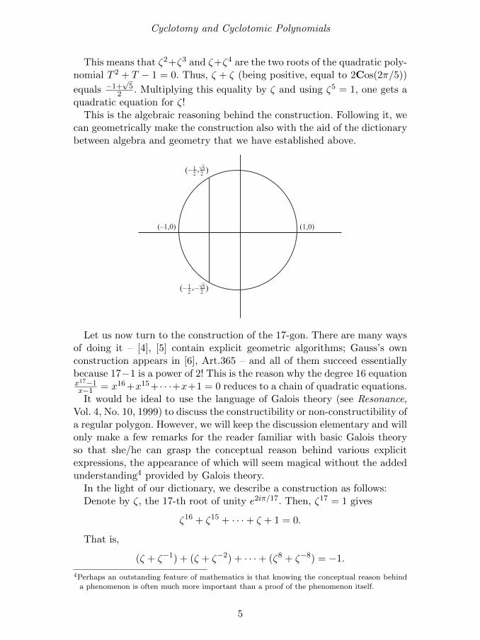
This means that ζ2+ζ3 and ζ+ζ4 are the two roots of the quadratic poly-nomial T 2 + T − 1 = 0. Thus, ζ + ζ (being positive, equal to 2Cos(2π/5))
equals −1+√
52 . Multiplying this equality by ζ and using ζ5 = 1, one gets a
quadratic equation for ζ!This is the algebraic reasoning behind the construction. Following it, we
can geometrically make the construction also with the aid of the dictionarybetween algebra and geometry that we have established above.
(–1,0) (1,0)
(– )1 √52 2,
(– – )1 √52 2,
Let us now turn to the construction of the 17-gon. There are many waysof doing it – [4], [5] contain explicit geometric algorithms; Gauss’s ownconstruction appears in [6], Art.365 – and all of them succeed essentiallybecause 17−1 is a power of 2! This is the reason why the degree 16 equationx17−1x−1 = x16 +x15 + · · ·+x+1 = 0 reduces to a chain of quadratic equations.It would be ideal to use the language of Galois theory (see Resonance,
Vol. 4, No. 10, 1999) to discuss the constructibility or non-constructibility ofa regular polygon. However, we will keep the discussion elementary and willonly make a few remarks for the reader familiar with basic Galois theoryso that she/he can grasp the conceptual reason behind various explicitexpressions, the appearance of which will seem magical without the addedunderstanding4 provided by Galois theory.
In the light of our dictionary, we describe a construction as follows:Denote by ζ, the 17-th root of unity e2iπ/17. Then, ζ17 = 1 gives
ζ16 + ζ15 + · · ·+ ζ + 1 = 0.
That is,
(ζ + ζ−1) + (ζ + ζ−2) + · · ·+ (ζ8 + ζ−8) = −1.
4Perhaps an outstanding feature of mathematics is that knowing the conceptual reason behind
a phenomenon is often much more important than a proof of the phenomenon itself.
5
Cyclotomy and Cyclotomic Polynomials
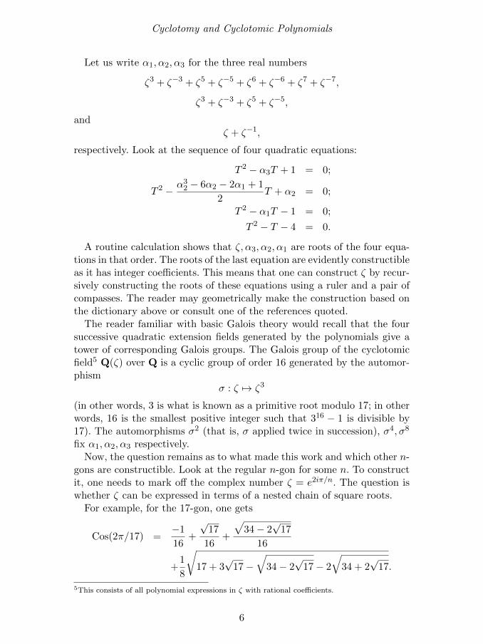
Let us write α1, α2, α3 for the three real numbers
ζ3 + ζ−3 + ζ5 + ζ−5 + ζ6 + ζ−6 + ζ7 + ζ−7,
ζ3 + ζ−3 + ζ5 + ζ−5,
andζ + ζ−1,
respectively. Look at the sequence of four quadratic equations:
T 2 − α3T + 1 = 0;
T 2 − α32 − 6α2 − 2α1 + 1
2T + α2 = 0;
T 2 − α1T − 1 = 0;
T 2 − T − 4 = 0.
A routine calculation shows that ζ, α3, α2, α1 are roots of the four equa-tions in that order. The roots of the last equation are evidently constructibleas it has integer coefficients. This means that one can construct ζ by recur-sively constructing the roots of these equations using a ruler and a pair ofcompasses. The reader may geometrically make the construction based onthe dictionary above or consult one of the references quoted.
The reader familiar with basic Galois theory would recall that the foursuccessive quadratic extension fields generated by the polynomials give atower of corresponding Galois groups. The Galois group of the cyclotomicfield5 Q(ζ) over Q is a cyclic group of order 16 generated by the automor-phism
σ : ζ 7→ ζ3
(in other words, 3 is what is known as a primitive root modulo 17; in otherwords, 16 is the smallest positive integer such that 316 − 1 is divisible by17). The automorphisms σ2 (that is, σ applied twice in succession), σ4, σ8
fix α1, α2, α3 respectively.Now, the question remains as to what made this work and which other n-
gons are constructible. Look at the regular n-gon for some n. To constructit, one needs to mark off the complex number ζ = e2iπ/n. The question iswhether ζ can be expressed in terms of a nested chain of square roots.
For example, for the 17-gon, one gets
Cos(2π/17) =−1
16+
√17
16+
√34− 2
√17
16
+1
8
√17 + 3
√17−
√34− 2
√17− 2
√34 + 2
√17.
5This consists of all polynomial expressions in ζ with rational coefficients.
6

Cyclotomy and Cyclotomic Polynomials
Thus, sin(2π/17) can also be expressed similarly.Of course, ζ is a root of the polynomial zn − 1, but it is a root of an
equation of smaller degree. What is the smallest degree equation of whichζ is a root? By the division algorithm, there is such a unique monic polyno-mial (that is, a polynomial with top coefficient 1) which divides any otherpolynomial of which ζ is a root. This polynomial is called a cyclotomic poly-nomial. The degree of this polynomial is of paramount importance becauseif it is a power of two, we know from our earlier discussion that ζ can beconstructed. The cyclotomic polynomials are useful in many ways and haveseveral interesting properties some of which will be discussed in the lastthree sections.
For a prime number p such that p − 1 is a power of 2, our discussionshows that the regular p-gon is constructible. Such a prime p is necessarilyof the form 22n + 1 since 2odd + 1 is always a multiple of 3. Fermat thoughtthat the numbers 22n + 1 are primes for all n. However, the only primes ofthis form found until now are 3, 5, 17, 257 and 65537(!). The number 225 +1was shown by Euler to have 641 as a proper factor. The primes of the form22n + 1 are called Fermat primes. For coprime numbers m and n, if them-gon and the n-gon are constructible, then so is the mn-gon. The reasonis, if we write ma+ nb = 1 for integers a, b, then
Cos
(2π
mn
)= Cos
(2πb
m+
2πa
n
)which is constructible when Cos
(2πbm
)and Cos
(2πan
)are. Thus, Gauss’s
analysis shows that if n is a product of Fermat primes and a power of2, the regular n-gon can be constructed by a ruler and compasses. Theconverse is also true; that is, if the regular n-gon is constructible, then n isof this special form. Gauss did not give a proof of this although he assertedit to be true – see [5]. The construction of the regular 257-gon was publishedin four parts in Crelle’s Journal. Details of the 65537-gon fill a whole trunkkept at the University of Gottingen!
We must see Gauss’s feat in the light of the fact that complex analysis wasin its infancy at that time. In fact, Gauss was the first one to give a rigorousproof (in his doctoral thesis) of the so-called fundamental theorem of alge-bra which asserts that every nonconstant complex polynomial has a root.
2. Abel’s Theorem for the Lemniscate
Abel earned fame by proving that the general equation of degree at leastfive is not solvable by a ‘formula’ involving only arithmetical operations andextraction of square roots, cube roots and higher roots of the coefficients– in other words, there is no such formula which can be prescribed so that
7
Cyclotomy and Cyclotomic Polynomials
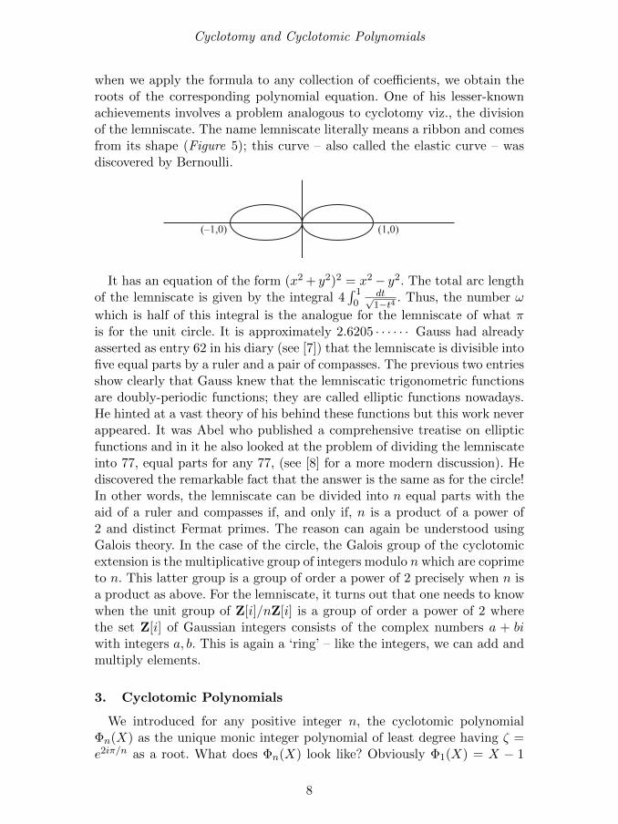
when we apply the formula to any collection of coefficients, we obtain theroots of the corresponding polynomial equation. One of his lesser-knownachievements involves a problem analogous to cyclotomy viz., the divisionof the lemniscate. The name lemniscate literally means a ribbon and comesfrom its shape (Figure 5); this curve – also called the elastic curve – wasdiscovered by Bernoulli.
(1,0)(–1,0)
It has an equation of the form (x2 + y2)2 = x2− y2. The total arc lengthof the lemniscate is given by the integral 4
∫ 10
dt√1−t4 . Thus, the number ω
which is half of this integral is the analogue for the lemniscate of what πis for the unit circle. It is approximately 2.6205 · · · · · · Gauss had alreadyasserted as entry 62 in his diary (see [7]) that the lemniscate is divisible intofive equal parts by a ruler and a pair of compasses. The previous two entriesshow clearly that Gauss knew that the lemniscatic trigonometric functionsare doubly-periodic functions; they are called elliptic functions nowadays.He hinted at a vast theory of his behind these functions but this work neverappeared. It was Abel who published a comprehensive treatise on ellipticfunctions and in it he also looked at the problem of dividing the lemniscateinto 77, equal parts for any 77, (see [8] for a more modern discussion). Hediscovered the remarkable fact that the answer is the same as for the circle!In other words, the lemniscate can be divided into n equal parts with theaid of a ruler and compasses if, and only if, n is a product of a power of2 and distinct Fermat primes. The reason can again be understood usingGalois theory. In the case of the circle, the Galois group of the cyclotomicextension is the multiplicative group of integers modulo n which are coprimeto n. This latter group is a group of order a power of 2 precisely when n isa product as above. For the lemniscate, it turns out that one needs to knowwhen the unit group of Z[i]/nZ[i] is a group of order a power of 2 wherethe set Z[i] of Gaussian integers consists of the complex numbers a + biwith integers a, b. This is again a ‘ring’ – like the integers, we can add andmultiply elements.
3. Cyclotomic Polynomials
We introduced for any positive integer n, the cyclotomic polynomialΦn(X) as the unique monic integer polynomial of least degree having ζ =e2iπ/n as a root. What does Φn(X) look like? Obviously Φ1(X) = X − 1
8
Cyclotomy and Cyclotomic Polynomials
and Φ2(X) = X + 1. Moreover, for a prime number p, Φp(X) = Xp−1 +Xp−2 + · · · + X + 1. For any n, the n-th roots of unity are the complexnumbers e2irπ/n; l ≤ r ≤ n. In other words, Xn − l =
∏nr=1(X − ζr) where
ζ = e2iπ/n. The crucial fact is that along with ζ, all the powers ζr with rcoprime 6 to n are the roots of Φn(X)! So,
Xn − 1 =∏d|n
∏(r,n)=d
(X − ζr) =∏d|n
Φd(X).
Here, we have denoted by (r, n) the greatest common divisor of r andn. Note that the degree of Φn(X) is the number of positive integers r ≤ nthat are coprime to n; this is usually denoted by φ(n), and called Euler’stotient. If we only look at the above expression, it is not clear that Φn(X)has integer coefficients. One may use elementary number theory to invertthe identity Xn− 1 =
∏d|n Φd(X). This is accomplished by what is known
as the Mobius inversion formula and, yields the identity
Φn(X) =∏d|n
(Xd − 1)µ(n/d)
where the Mobius function µ(m) is defined to take the value 0, 1 or −1according as whether m is divisible by a square, is a square-free product ofan even number of primes, or is a square-free product of an odd numberof primes. The inversion formula is a very easy and pleasant exercise inelementary number theory. Note that from the above expression, it is notclear that the fractional expression on the right side is indeed a polynomialbut that this follows from induction on n using the expression Xn − 1 =∏d|n Φd(X).By observing this among the cyclotomic polynomials Φp(X) for prime
p and for Φn(X) for small n, an interesting feature is that the coefficientsseem to be among 0, 1 and −1. One might wonder whether this is trueabout Φn(X) for any n. It turns out that Φ105 has one coefficient equalto 2. This is not an aberration. Indeed, using some nontrivial results onhow prime numbers are distributed, one can show that every integer occursamong the coefficients of the cyclotomic polynomials!
4. Infinitude of Primes Ending in 1
11, 31, 41, 61, 71, 101, · · · are primes – where does it stop? Are there in-finitely many primes ending in 1? Equivalently, does the arithmetic pro-gression 10n + 1;n ≥ 1 contain infinitely many prime numbers? Anyprime number other than 2 must obviously end in 1, 3, 7 or 9. The natural
6These are the primitive n-th roots of unity i.e., they are notm-th roots of unity for any smallerm.
9

Cyclotomy and Cyclotomic Polynomials
question is whether there are infinitely many of each type? The answer is‘yes’ by a deep theorem due to Dirichlet – infinitely many primes occur inany arithmetic progression a+ nd;n ≥ 1 with a, d coprime.
If d is a positive integer, then for the arithmetic progression nd + 1;n ≥ 1, one can use cyclotomic polynomials to prove this! This is notsurprising because we have already noted in the last section that cyclotomicpolynomials are related to the way prime numbers are distributed. Let usprove this now.
Suppose p1, p2, · · · , pr are prime numbers in this arithmetic progression.We will use cyclotomic polynomials to produce another prime p in thisprogression different from the above pi’s. This would imply that there areinfinitely many primes in such a progression. We will use the simple obser-vation that a polynomial p(X) with integer coefficients has the propertythat p(m)− p(n) is an integer multiple of m− n.
Consider the number N = dp1p2 · · · pr. Then, for any integer n, the twovalues Φd(nN) and Φd(0) differ by a multiple of N . But, Φd(0) is an integerwhich is also a root of unity and must, therefore, be ±1. Moreover, asn → ∞, the values Φd(nN) → ∞ as well since Φd is a nonconstant monicpolynomial. In other words, n > 0, the integer Φd(nN) has a prime factorp. As Φd(nN) is ±1 modulo any of the p1, p2, · · · , pr and modulo d, theprime p is different from any of the pi’s and does not divide d. One mightwonder which primes divide some value Φd(a) of a cyclotomic polynomial.The answer is that these are precisely the primes occurring in the arithmeticprogression nd+ 1;n > 0. To show this, we use the idea that the nonzerointegers modulo p form a group of order p − 1 under the operation ofmultiplication modulo p. So, it is enough to prove that if p divides Φd(a)for some integer a, then a has order d in this group (for, then Lagrange’stheorem of finite group theory tells us that d divides the order p − 1 ofthe group, which is just re-stating that p is in the arithmetic progressionnd+1;n > 0. Let us prove this now. Since Xd−1 =
∏l|d Φl(X), it follows
that p which divides Φd(a) has to divide ad−1 also. If d were not the orderof a, let k divide d with k < d and p divides ak−1. Once again, the relationak − 1 =
∏l|k Φl(a) shows that p divides Φl(a) for some positive integer l
dividing k. Therefore, p divides both Φd(a+ p) and Φl(a+ p). Now,
(a+ p)d − 1 =∏m|d
Φm(a+ p) = Φd(a+ p)Φl(a+ p) (other terms).
The expression on the right hand side is divisible by p2. On the otherhand, the left side is equal, modulo p2, to ad + dpad−1− 1. Since p2 dividesad−1, it must divide dpad−1 as well. This is clearly impossible since neithera nor d is divisible by p. This proves that any prime factor p of Φd(nN)
10

Cyclotomy and Cyclotomic Polynomials
occurs in the arithmetic progression 1+nd;n > 0 and thereby, proves theinfinitude of the primes in this progression. Interestingly, Euclid’s classicalproof of the infinitude of prime numbers is the special case of the aboveproof where we can use d = 2.
5. Sum of Primitive Roots
For a prime number p, Gauss defined a primitive root modulo p to be aninteger a whose multiplicative order modulo p is p− 1. In other words, a isa generator of the multiplicative group of non-zero integers modulo p. Moregenerally, for a positive integer n, every integer a coprime to n is such thataφ(n) is 1 modulo n. A primitive root modulo n is an integer a such thatφ(n) is the smallest r > 0 for which ar is 1 modulo n. Gauss also showedthat primitive roots modulo n exist if, and only if, n is 2, 4, pa or 2pa forsome odd prime p.
For instance, the primitive roots modulo 5 among the integers 1 to 4 are2 and 3. Their sum is 0 modulo 5. Now, look at the primitive roots modulo7 among 1 to 6. These are 3 and 5. Modulo 7, these sum to 1. What about11? The primitive roots here are 2, 6, 7 and 8 and these give the sum 1modulo 11. What is the pattern here? Without letting out the secret, letus go on to investigate the problem for a general prime p.
When is an integer modulo p a primitive root? As we already observed,an integer a is a primitive root modulo p precisely when p divides theinteger Φp−1(a). This means when the polynomial Φp−1(X) is regarded as apolynomial with coefficients integers modulo p, a is a root. Hence the sumof all the primitive roots modulo p is simply the sum modulo p of the rootsof Φp−1 modulo p. As we will prove below, the above sum is µ(p−1), whereµ(n) is the Mobius function.
6. Cyclotomic Polynomials and Ramanujan Sums [9]
In his famous paper ([10]), Ramanujan discussed the properties of certainfinite sums – the so-called Ramanujan sums. Even though Dirichlet andDedekind had already considered these sums in the 1860’s, according toG H Hardy, “Ramanujan was the first to appreciate the importance ofthe sum and to use it systematically.” Ramanujan sums play a key role inthe proof of a famous result due to Vinogradov asserting that every largeodd number is the sum of three primes. These sums have numerous otherapplications in diverse branches of mathematics as well as in some parts ofphysics. So, what are these sums?
For integers n ≥ 1, k ≥ 0, the sum
cn(k) =∑
(r,n)=1;r≤n
e2ikrπ/n
11

Cyclotomy and Cyclotomic Polynomials
is called a Ramanujan sum. In other words, it is simply the sum of the k-thpowers of the primitive n-th roots of unity – ‘primitive’ here means that thenumber is not an m-th root of unity for any m < n. Note that the primitiven-th roots of unity are the numbers e2ikrπ/n for all those r ≤ n which arerelatively prime to n.
The first remarkable property cn(k) have is that they are integers. Ra-manujan showed that several arithmetic functions (that is, functions de-fined from the set of positive integers to the set of complex numbers) have‘Fourier-like’ of expansions in terms of the sums; hence, nowadays these ex-pansions are known as Ramanujan expansions. They often yield very prettyelementary number-theoretic identities. Recently, the theory of group rep-resentations of the permutation groups (specifically, the so-called super-character theory has been used to re-prove old identities in a quick wayand also, to discover new identities.
It is convenient to write
∆n = e2irπ/n : (r, n) = 1, 1 ≤ r ≤ n.
Then, the set of all n-th roots of unity e2ikπ/n : 0 ≤ k < n is a unionof the disjoint sets ∆d as d varies over the divisors of n. This is because ann-th root of unity is a primitive d-th root of unity for a unique divisor d ofn. It is also convenient to introduce the ‘characteristic’ function δk|n whichhas the value 1 when k divides n and the value 0 otherwise. Before statingsome properties of the ck(n)’s, let us recall two arithmetic functions whichare ubiquitous in situations where elementary number-theoretic counting isinvolved. The first one is Euler’s totient function
φ(n) = |r : 1 ≤ r ≤ n, (r, n) = 1|.
The other arithmetic function is the Mobius function defined byµ(1) = 1, µ(n) = (−1)k or 0 for n > 1 according as to if n is a square-free
integer that is a product of k distinct primes or otherwise.The Mobius function keeps tab when we use the principle of inclusion-
exclusion to do counting. The basic result which can be easily proved byinduction on the number of prime factors, is the Mobius inversion formula:
If g is an arithmetic function and
f(n) =∑d|n
g(d),
then
g(n) =∑d|n
f(d)µ(n/d).
12

Cyclotomy and Cyclotomic Polynomials
With these notations, here are some elementary properties of the Ra-manujan sums.
(i) cn(k) = cn(−k) = cn(n− k).(ii) cn(0) = φ(n) and cn(1) = µ(n).
(iii) cn(ks) = cn(k) if (s, n) = 1; in particular, cn(s) = µ(n) if (s, n) = 1.(iv) cn(k) = cn(k′) if (k, n) = (k′, n); in particular, cn(k) ≡ cn(k′) mod n
if k ≡ k′ mod n.(v)
∑n−1k=0 cn(k) = 0.
(vi)∑
d|n cd(k) = δn|kn and cn(k) =∑
d|n dµ(n/d)δd|k =∑
d|(n,k) dµ(n/d);
in particular, for prime powers pr, we have cpr(k) = pr − pr−1 if pr|k;= −pr−1 if pr−1||k; and = 0 otherwise.
(vii) cmn(k) = cm(k)cn(k) if (m,n) = 1.(viii)
∑nk=1 cm(k)cn(k) = δmnnφ(n).
The property (vi) shows that these sums actually have integer values.The proof of (i) follows already from the definition and, so do the first
parts of (ii) and (iii). The second parts of (ii), (iii) as well as the assertions(iv) and (vii) will follow from (vi). We shall prove (v) and (vi).
For (v), we have
n−1∑k=0
cn(k) =n−1∑k=0
∑ζ∈∆n
ζk =∑ζ∈∆n
n−1∑k=0
ζk = 0
where the last equality is because
n−1∑k=0
ζk =1− ζn
1− ζ= 0
for each ζ ∈ ∆n.For proving (vi), we note that the second statement follows from the first
by the Mobius inversion formula. Let us prove the first one now. We have
∑d|n
cd(k) =∑d|n
∑ζ∈∆d
ζk =n−1∑m=0
e2imkπ/n
because, as we observed, the disjoint union of ∆d as d varies over thedivisors of n is the set of all n-th roots of unity. Now, if the above sum∑n−1
m=0 e2imkπ/n is multiplied by e2ikπ/n, we get the same sum which means
that it is equal to 0 unless n|k. When k|n, the sum is clearly equal to n.This proves (vi).
The other parts easily follow from (vi).
13

Cyclotomy and Cyclotomic Polynomials
The equality cn(k) =∑
d|n dµ(n/d)δd|k is very useful.7 For instance, if nis a prime power pr, as we noted above in (vi), we have
cpr(k) = prδpr|k − pr−1δpr−1|k.
Using this expression in (vii) above, we get
ck(n) =µ( k
(k,n))φ(k)
φ( k(k,n))
.
The right hand side was studied by R D Von Sterneck in 1902 and isknown by his name. The equality above itself was known before Ramanujanand is due to J C Kluyver in 1906.
7. Connection of Ramanujan Sums with CyclotomicPolynomials
The cyclotomic polynomials Φn(x) =∏ζ∈∆n
(x−ζ) have some fascinatingproperties and have surprising consequences (see [9], where applicationssuch as the infinitude of primes in arithmetic progressions of the form 1 +an are proved). We have:
xn − 1 =∏d|n
∏ζ∈∆d
(x− ζ) =∏d|n
Φd(x)
and – by Mobius inversion, we deduce
Φn(x) =∏d|n
(xd − 1)µ(n/d).
Taking the logarithmic derivative, we obtain
Φ′n(x)
Φn(x)=∑d|n
dxd−1µ(n/d)
xd − 1.
Multiplying by x(xn − 1), we get a polynomial in x, viz.,
x(xn − 1)Φ′n(x)
Φn(x)=∑d|n
dµ(n/d)(xd + x2d + · · ·+ xn).
7Note that even computationally the defining sum for cn(k) requires approximately n operations
whereas the other sum requires roughly log(n) operations.
14

Cyclotomy and Cyclotomic Polynomials
Thus, the coefficient of xk in the polynomial on the right is∑
d|(n,k) dµ(n/d),which is simply the Ramanujan sum cn(k). Hence, we have:
Proposition. For each k < n, the Ramanujan sum cn(k) is the coeffi-
cient of xk−1 in the polynomial (xn − 1)Φ′n(x)Φn(x) .
Note a special case of the above discussion.The sum of the roots of Φn(X) is cn(1) = µ(n) as seen above. In partic-
ular, if n = p− 1 for a prime p, the sum of primitive roots modulo p is thesum of the roots of the polynomial Φp−1(X) modulo p, which is thereforeµ(p− 1). More generally, the sum of the r-th powers of the primitive rootsmod p equals the Ramanujan sum cp−1(r).
8. Equal Sums of Powers via Cyclotomic Polynomials
One has the elementary identity
13 + 33 + · · ·+ n3 = (1 + 2 + · · ·+ n)2.
By raising both sides to the k-th power, we have the identity
(13 + 23 + 33 + · · ·+ n3)k = (1 + 2 + 3 + · · ·+ n)2k.
Are there other such identities? It turns out that there are no others. Weshall prove this now using cyclotomic polynomials. To be more precise, letus set up the notation
pr(n) = 1r + 2r + · · ·+ nr.
for any natural numbers n, r. Let us look for natural numbers r1 < r2 <· · · < rk and s1 < s2 < · · · < sl different from the ri’s and, also some naturalnumbers a1, a2, · · · , ak, b1, b2, · · · , bl such that, for any natural number n,one has identities
pr1(n)a1pr2(n)a2 · · · prk(n)ak = ps1(n)b1ps2(n)b2 · · · psl(n)bl .
If we have such an identity, then (for n = 2),
(1 + 2r1)a1 · · · (1 + 2rk)ak = (1 + 2s1)b1 · · · (1 + 2sl)bl · · · (A)
Now, we look at the larger number among rk or sl, say sl. If sl ≤ 3, thenthe identity can be shown to be just
p3(n)a = p1(n)2a,
that is,(13 + 23 + 33 + · · ·+ n3)a = (1 + 2 + 3 + · · ·+ n)2a
15

Cyclotomy and Cyclotomic Polynomials
which we have already seen. This is an easy check. Now, let us supposesl > 3. Below, we will prove the nice fact that any number of the form1 + 2b with b > 3 always has a prime factor which is not a factor of any1 + 2c for any c < b. This beautiful observation was first made by A SBang 120 years ago. This observation shows immediately that an equalityof the form (A) cannot hold good because the prime factor p of the largest1 + 2sl cannot divide any term on the left hand side. Seeing why Bang’sobservation is valid requires some discussion about cyclotomic polynomialswhich we proceed to do now.
Generally, if one has an infinite sequence of natural numbers u1 < u2 <u3 < · · · such that for every n, there exists a prime factor of un which doesnot divide um for every m < n usually called a primitive prime divisor ofun. From any such sequence admitting primitive prime divisors, we have aproof of infinitude of primes because we find at least one new prime divisorat each step as we move along the sequence of un’s.
We show now that the sequence 2n + 1n>3 has primitive divisors.An advantage of knowing that the cyclotomic polynomials Φn(x) have in-
teger coefficients is the following. For any integer a and any natural numbern, one has
an − 1 =∏d|n
Φd(a)
which is a product of integers. Thus, if p is any prime dividing an − 1 forsome a, then p divides Φd(a) for some d|n.
Now, we make the following interesting assertion :
Proposition. Let n > 2. If p is a prime dividing Φn(a) for some integera > 1, then p divides an−1 and in this case n is the smallest natural numbersuch that p divides an − 1 unless p|n in which case the smallest number isof the form n/pi for some i ≥ 1. In the latter case, p is the largest primedividing n. Finally, given a > 1 and n > 2, if there are no primes p forwhich a has order n mod p, then Φn(a) is actually a prime.
Let us prove this. Indeed, p divides an − 1 since Φn(a) divides an − 1.Also, if p divides am − 1 for some m < n as well, then p divides a(m,n) − 1where (m,n) is the GCD of m and n.
Therefore, if n were not the smallest for which p divides an−1, we wouldhave a factor d of n such that d < n and p|(ad − 1). As d < n and d|n,there is some prime q such that qd|n. Thus, d divides n/q and so p dividesan/q − 1. Writing b = an/q, we see that b leaves a remainder 1 on divisionby p. So, we have
an − 1
an/q − 1=bq − 1
b− 1= 1 + b+ b2 + · · ·+ bq−1
16

Cyclotomy and Cyclotomic Polynomials
leaves a remainder of q on division by p. On the other hand, the left handside is a multiple of Φn(a) which is a multiple of p. Thus, we must havethat p = q and that it divides n.
This also shows that an/q − 1 is not a multiple of p for any prime divisorq 6= p of n. Thus, the order of a mod p (which means the smallest naturalnumber d such that p divides ad − 1) is either n or of the form n/pi for somei ≥ 1.
To say that when the order of a mod p is < n, then the prime p (whichwe have shown to be a divisor of n) is the largest prime divisor, we need touse Fermat’s little theorem.
In the case when the order of a mod p is < n, we have seen that it isof the form n/pi. Thus, n/pi divides p− 1 which means every other primedivisor of n is < p. This proves the proposition except for the last assertion.
To see that the last assertion of the proposition also holds, consider n > 2,a > 1 and a prime divisor p of Φn(a). Under the hypothesis that there areno primes modulo which a has order n, we have seen that p is the largestprime dividing n and that Φn(a) = pk for some k ≥ 1. We assert that k = 1.Now, Φn(a) divides
an − 1
an/p − 1= 1 + an/p + a2n/p + · · ·+ a(p−1)n/p.
As an/p = 1 + pb for some b, the right hand side above is
1 + (1 + pb) + · · ·+ (1 + pb)(p−1)
= p+ p(b+ 2b+ · · ·+ (p− 1)b) + p2c = p+ p2d
for some c, d if p > 2.Therefore, p2 does not divide Φn(a); hence Φn(a) = p.When p = 2, the argument is again easy remembering that n > 2 is a
power of 2 as p is the largest prime divisor of n.This proves the proposition.How does one relate what we need about primitive prime divisors for
the sequence 2n + 1n>3 with the above discussion? For each n > 3, if wefind a prime p such that the order of 2 mod p is 2n, then from (22n − 1)= (2n − 1)(2n + 1), we would have p|(2n + 1) because p does not divide2n − 1. Also, if p divided 2m + 1 for some m < n, then it would divide22m − 1 which would contradict the fact that the order of 2 mod p is 2n.
In order to get a prime p such that 2 has order 2n mod p, we need to geta prime p dividing Φ2n(2) and not dividing 2n. If there is no such prime,then as we saw in the discussion above, we must have that Φ2n(2) = p isthe largest prime dividing n, and p is odd. Writing 2n = pid with d dividingp− 1. On the other hand,
Φ2n(2) =Φd(2
pi)
Φd(2pi−1)
=
∏φ(d)r=1 (bp − ζr)∏φ(d)r=1 (b− ζr)
> (bp − 1
b+ 1)φ(d),
17

Cyclotomy and Cyclotomic Polynomials
where b = 2pi−1
and ζr are the φ(d) primitive d-th roots of unity (the rootsof Φd(x)).
As bp − 1 ≥ bp−2(b2 − 1), the right side above is > b(p−2)φ(d)(b − 1)φ(d).As b ≥ 2, this last expression is at least 2p−2. Therefore, we have
p = Φ2n(2) > 2p−2,
which is possible only if p = 3. In that case we must also have 2n = 6which we rule out. In other words, when n > 3, then there does exista prime divisor p of Φ2n(2) which does not divide n; the above discussionthen shows that n is the smallest natural number for which p divides 2n+1.This finishes the whole argument.
9. Cyclotomic Polynomials and a Problem in Geometry
Let us first start with the following simple question. On the unit circle,take n points dividing the circumference into n equal parts. From one ofthese n points, draw the n−1 chords joining it to the other points. It is easyto see that the product of the lengths of these chords is n. A more difficultproblem is to start from one of the points and – going in one direction (say,the anticlockwise direction) – drawing the chords joining it to the k-th pointfrom it for each k relatively prime to n, what is the product of the lengthsof these chords in this case?
We prove:Let n > 1 and let P1, · · · , Pn be points on a circle of radius 1 dividing
the circumference into n equal parts. Then, we have :The product of lengths
∏(l,n)=1,l<n |P1Pl+1| = p or 1 accordingly as to
whether n = pk for a prime p or n is not a power of a prime.
We may assume that the origin is the centre and that points are Pd+1
= e2idπ/n for d = 0, 1, · · · , n − 1. Note that the product of lengths of allthe chords P1Pi is simply
∏n−1d=1 |1− e2idπ/n|. Since the polynomial 1 +X +
· · ·+Xn−1 has as roots all the n-th roots of 1 excepting 1 itself, we have
n−1∏d=1
(1− e2idπ/n) = n,
by evaluating at X = 1. Notice that we have the equality∏n−1d=1 (1−e2idπ/n)
= n as complex numbers; that is, even without considering absolute values.Now, let us consider our problem. Here, the product under consideration
is ∏(d,n)=1
|1− e2idπ/n|.
18

Cyclotomy and Cyclotomic Polynomials
First, let us look at the case when n = pk for some prime p. Then,
∏(d,pk)=1,d<pk
|1− e2idπ/pk | =∏pk−1d=1 |1− e
2idπ/pk |∏dp<pk |1− e2idpπ/pk |
=pk
pk−1= p.
Now, suppose that n has at least two prime factors.Let us start with the identity
∏n−1d=1 (1− e2idπ/n) = n.
If p is a prime dividing n, suppose pk is the highest power of p dividing n.Then, the product
∏n−1d=1 (1− e2idπ/n) contains the products of terms corre-
sponding to d running through multiples of n/pk; that is,∏pk−1d=1 (1−e2idπ/pk)
(which is pk). We observe that factors occurring for a different prime qdividing n are disjoint from those occurring corresponding to p. There-fore, the factors corresponding to the various primes dividing n contribute∏pk||n p
k = n.On removing these factors corresponding to each prime divisor of n, we
will get∏d∈D(1 − e2idπ/n) = 1, where D consists of those d for which
e2idπ/n does not have prime power order. Thus, if d ∈ D, then 1 − e2idπ/n
is a unit since n is not a prime power. Therefore, 1− e2iπ/n is a unit in thecyclotomic field Q(e2iπ/n). From Galois theory, we have that the product∏
(d,n)=1(1− e2idπ/n) is the norm of 1− e2iπ/n from Q(e2iπ/n) to Q. As this
element is a unit, this product is ±1. Hence we get∏
(d,n)=1 |1−e2idπ/n| = 1which proves our assertion in the case when n is not a prime power. Theproof is complete.
In the above proof, the second part can also be deduced from the firstpart of the proof in a different fashion as follows.
Writing P (n) =∏n−1l=1 (1 − ζ l) and Q(n) =
∏(d,n)=1(1 − ζd), where ζ =
e2iπ/n, we can see that
P (n) =∏r|n
Q(r).
By Mobius inversion, Q(n) =∏d|n P (d)µ(n/d) =
∏d|n d
µ(n/d) by the sim-pler first assertion observed at the beginning of the pr of the proposition.The function
logQ(n) =∑d|n
µ(n/d) log(d),
can be identified with the so-called von Mangoldt function Λ(n) whichis defined to have the value log(p) if n is a power of p and 0 otherwise.Using this identification, exponentiation gives also the value asserted in theproposition; viz., Q(n) = p or 1 according as to whether n is a power of aprime p or not.
19

Cyclotomy and Cyclotomic Polynomials
To see why Λ(n) =∑
d|n µ(n/d) log(d), we write n =∏p|n p
vp(n) and notethat
log(n) =∑p|n
vp(n) log(p)
But, the right hand side is clearly∑
d|n Λ(d). Hence, Mobius inversionyields
Λ(n) =∑d|n
log(d)µ(n/d).
We shall use the solution of the above elementary geometric problem(obtained using cyclotomic polynomials) to unearth interesting informationabout the so-called cyclotomic field Q(ζn) which consists of polynomialexpressions in ζn = e2iπ/n. This section requires a bit of background in basicfield theory. It also implies by the so-called Dedekind–Kummer criterion,the well-known fact that the primes ramifying in Q(ζn) are exactly thosewhich divide n.
Discriminant of Q(ζn). Let n > 2 be a positive integer and ζn be aprimitive n-th root of unity. Then, the discriminant of the cyclotomic field
is (−1)φ(n)/2 nφ(n)∏p|n p
φ(n)/(p−1) .
Recall that the ring OK of algebraic integers of K = Q(ζn) is Z[ζn].The minimal polynomial of ζn is the cyclotomic polynomial
Φn(X) =∏
(r,n)=1
(X − ζrn).
Thus, the discriminant of OK is that of the polynomial Φn up to sign.The polynomial Φn has another expression Φn(X) =
∏d|n(Xd − 1)µ(n/d)
which is obtained by Mobius inversion formula to the decomposition
Xn − 1 =∏d|n
Φd(X).
Let us prove the first result.Since
Φn(X) =∏d|n
(Xd − 1)µ(n/d) = (Xn − 1)∏
d|n,d<n
(Xd − 1)µ(n/d),
we may write
Ψ(X) :=Xn − 1
Φn(X)=
∏d|n,d<n
(Xd − 1)−µ(n/d).
20

Cyclotomy and Cyclotomic Polynomials
Now, differentiating Xn − 1 = Φn(X)Ψ(X) and putting X = ζn, we getnζ−1
n = Φ′n(ζn)Ψ(ζn).We have the discriminant d(K) = ±NK/QΦ′n(ζn) = ±nφ(n)NK/Q(Ψ(ζn))−1.
Now Ψ(ζn)−1 =∏d|n,d<n(ζdn−1)µ(n/d) which is convenient to write (using
n/d instead of d) as:
Ψ(ζn)−1 =∏
d|n,d>1
(ζn/dn − 1)µ(d),
Separating the terms corresponding to µ(d) = 1 and to µ(d) = −1, wehave
Ψ(ζn)−1 =
∏d|n,d>1,µ(d)=1(ζ
n/dn − 1)∏
d|n,d>1,µ(d)=−1(ζn/dn − 1)
.
Now, for each divisor d of n, ζn/dn is a primitive d-th root of unity. By
proposition 1 above, 1−ζn/dn is a unit unless d is a prime power. In the aboveexpression for Ψ(ζn)−1, a nontrivial term in the denominator correspondsto µ(d) = −1 which can happen for a prime power d only if d is prime. Inthe numerator, the condition µ(d) = 1 cannot happen for any prime powerd. In other words,
Ψ(ζn)−1 = (unit).∏p|n
(ζn/pn − 1)−1.
So, its norm is ±∏p|nNK/Q(ζ
n/pn − 1)−1 as units have norm ±1.
As ζn/pn is a primitive p-th root of unity, it is in the subfield Q(ζp) gen-
erated by a primitive p-th root of unity, and we have
NK/Q(ζn/pn − 1) = (NQ(ζp)/Q(ζp − 1))[K:Q(ζp)] = (±p)φ(n)/(p−1).
Thus, we get
d(K) = ± nφ(n)∏p|n p
φ(n)/(p−1).
Finally, it is well-known (and easy to deduce from the definition) thatfor any number field L, the discriminant d(L) has sign (−1)s where s isthe number of complex places of L. Our field K = Q(ζn) has s = φ(n)/2because primitive n-th roots of unity are all complex.
10. Reducibility of Cyclotomic Polynomials Modulo Primes
The cyclotomic polynomial Φn is the monic, irreducible polynomial ofa primitive n-th root of unity but it may happen to be reducible modulocertain primes. In this section, we investigate when this happens.
21

Cyclotomy and Cyclotomic Polynomials
We recall:
For a positive integer n > 2, if disc(Φn) is a perfect square, then Φn isreducible modulo every prime.
This proof is a standard application of Galois theory. Indeed, it is well-known that if the discriminant of a Galois extension is a square, its Galoisgroup would be contained in the subgroup of even permutations ([1], Lemma12.3). So, if Φn were irreducible modulo some prime p, then the reductionof Φn mod p generates over Fp a Galois extension of degree φ(n); the Galoisgroup would contain a φ(n)-cycle which is an odd permutation since φ(n)is even for n
We prove:
For n > 2, the polynomial Φn is reducible modulo every prime if, andonly if, disc(Φn) is a perfect square. If disc(Φn) is not a perfect square –which happens if, and only if, n = 4, pk or 2pk – then there are infinitelymany primes p such that Φn is irreducible modulo p.
Let us prove this now.We have already seen that if disc(Φn) is a perfect square in Z, then
Φn is reducible modulo every prime. Conversely, suppose disc(Φn) is not a
perfect square. Then, looking at the expression (−1)φ(n)/2 nφ(n)∏p|n p
φ(n)/(p−1) for
the discriminant, we shall deduce that n = 4, pk or 2pk for some odd prime.Indeed, write
n = pα11 pα2
2 · · · pαrr .
Firstly, if n is odd and r > 1, clearly,
φ(n)
2=
∏ri=1 p
αi−1i (pi − 1)
2,
is even and the power of pi dividing the discriminant is(αi(pi − 1)− 1
)( r∏k=1
pαk−1k
)(∏j 6=i
(pj − 1)
),
which is even.Thus, if n > 2 is odd, then the discriminant is a perfect square unless
n = pk.If n = 2pα1
1 · · · pαrr for some odd primes, Φn = Φn/2 and the discriminant
is a perfect square excepting the case r = 1; i.e., n = 2pk.Now, if n = 2αpα1
1 · · · pαrr with either α > 2 or α = 2 and r ≥ 1, thenagain the powers of 2 and each pi dividing the discriminant are all even.
Thus, the exceptional case is n = 4.Therefore, we have deduced that the expression for discriminant is a
perfect square excepting the cases n = 4, pk and 2pk for an odd prime.
22

Cyclotomy and Cyclotomic Polynomials
These exceptional cases are when the Galois group of the cyclotomic fieldis cyclic.
The Galois group of Φn over Q is a cyclic group of order φ(n) and con-tains a φ(n)-cycle. By the Frobenius density theorem discussed in a laterchapter, there are infinitely many prime numbers l such that the decompo-sition group at l is cyclic of order φ(n) which means that Φn modulo l isirreducible and generates the extension of degree φ(n) over Fl. This provesthe proposition.
References
[1] P Morandi, Field and Galois theory, Graduate texts in Mathematics167, Springer-Verlag, 1996.
[2] M Ram Murty and J Esmonde, Problems in Algebraic Number Theory,Graduate Texts in Mathematics 190, Springer-Verlag, New York, 2005.
[3] M Artin, Algebra, Prentice Hall, 1991.[4] D Suryaramana, Resonance, Vol. 2, No. 6, 1997.[5] Ian Stewart, Gauss, Scientific American, 1977.[6] C F Gauss, Disquisitiones Arithmeticae, English Edition, Springer,
1985.[7] J Gray, English translation and commentary on Gauss’s mathematical
diary, Expo. Math., Vol. 2, 1984.[8] M Rosen, Amer. Math. Monthly, 1981.[9] B Sury, Ramanujan’s Awesome Sums,Mathematics Newsletter,
Vol. 24, no. 2, pp. 31–36, September 2013.[10] S Ramanujan, On certain trigonometrical sums and their applications
in the theory of numbers, Trans. Cambridge Philos. Soc., Vol. 22,No. 13, 259-276, 1918.
23


Polynomials with Integer Values
A quote attributed to the famous mathematician L Kronecker is ‘DieGanzen Zahlen hat Gott gemacht, alles andere ist Menschenwerk.’ A trans-lation might be ‘God gave us integers and all else is man’s work.’ All of usare familiar already from middle school with the similarities between theset of integers and the set of all polynomials in one variable. A paradigmof this is the Euclidean (division) algorithm. However, it requires an as-tute observer to notice that one has to deal with polynomials with real orrational coefficients rather than just integer coefficients for a strict anal-ogy. There are also some apparent dissimilarities – for instance, there is nonotion among integers corresponding to the derivative of a polynomial. Inthis discussion, we shall consider polynomials with integer coefficients. Ofcourse a complete study of this encompasses the whole subject of algebraicnumber theory, one might say. Most of this article sticks to fairly elemen-tary methods (in fact, other than the discussion on Schur’s theorem) toaddress a number of rather natural questions. To give a prelude, since thesquare of a polynomial with integer coefficients takes perfect square valuesat all integer points, one such natural question might be “if an integralpolynomial takes only values which are perfect squares, then must it be thesquare of a polynomial? ” Note that for a natural number n, the polynomial(Xn
)= X(X−1)···(X−n+1)
n(n−1)···1 takes integer values at all integers although it doesnot have integer coefficients.
1. Prime Values and Irreducibility
The first observation about polynomials taking integral values is:
Lemma 1.1. A polynomial P takes integer values at all integer points if,and only if, P (X) = a0 + a1
(X1
)+ · · ·+ an
(Xn
)for some ai in Z.
Proof. The sufficiency is evident. For the converse, we first note thatany polynomial whatsoever can be written in this form for some n andsome (possibly non-integral) a′is. Writing P in this form and assuming thatP (Z) ⊂ Z, we have
P (0) = a0 ∈ Z
P (1) = a0 + a1 ∈ Z
P (2) = a0 + a1
(21
)+ a2 ∈ Z
and so on. Inductively, since P (m) ∈ Z∀m, we get an ∈ Z ∀ n.
The chapter is a modified version of an article that first appeared in Resonance, Vol. 6, No. 9,
pp. 46–60, September 2001.
25

Polynomials with Integer Values
COROLLARY 1.2
If a polynomial P takes integers to integers and has degree n, then n!P (X)∈ Z[X].
Lemma 1.3. A nonconstant integral polynomial P (X) cannot take onlyprime values.
Proof. If all values are composite, then there is nothing to prove. So,assume that P (a) = p for some integer a and prime p. Now, as P is non-constant, lim
n→∞|P (a+np)| =∞. So, for big enough n, |P (a+np)| > p. But
P (a+ np) ≡ P (a) ≡ 0 mod p, which shows P (a+ np) is composite.
Remark 1.4. Infinitely many primes can occur as integral values of apolynomial. For example, if (a, b) = 1, then the well-known (but deep)Dirichlet’s theorem on primes in progression shows that the polynomialaX+b takes infinitely many prime values. In general, it may be very difficultto decide whether a given polynomial takes infinitely many prime values.For instance, it is not known if X2 + 1 represents infinitely many primes.In fact, there is no known polynomial of degree ≥ 2 which takes infinitelymany prime values.
Lemma 1.5. If P is a nonconstant polynomial that takes integers to inte-gers, the number of prime divisors of its value set P (m)m∈Z, is infinitei.e. not all terms of the sequence P (0), P (1), · · · can be built from finitelymany primes.
Proof. It is clear from the note above that it is enough to prove this for
P (X) ∈ Z[X], which we will henceforth assume. Now, P (X) =n∑i=0
aiXi
where n ≥ 1. If a0 = 0, then clearly P (p) ≡ 0 mod p for any prime p. Ifa0 6= 0, let us consider for any integer t, the polynomial
P (a0tX) =
n∑i=0
ai(a0tX)i = a0
1 +
n∑i=1
aiai−10 tiXi
= a0Q(X).
There exists some prime number p such that Q(m) ≡ 0 mod p for somem and some prime p, because Q can take the values 0,1,−1 only at finitelymany points. Since Q(m) ≡ 1 mod t, we have (p, t) = 1. Then P (a0tm) ≡0 mod p. Since t was arbitrary the set of p arising in this manner is infinite.
Remark 1.6. (a) Note that it may be possible to construct infinitely manyterms of the sequence P (m)m∈Z using only a finite number of primes.For example take (a, d) = 1, a ≥ d ≥ 1. Since, by Euler’s theorem, aϕ(d) ≡1 mod d, the numbers a(aϕ(d)n−1)
d ∈ Z ∀ n. For the polynomial P (X) =
dX + a, the infinitely many values P (ad(aϕ(d)n − 1)) = aϕ(d)n+1 have onlyprime factors coming from primes dividing a.
26

Polynomials with Integer Values
(b) In order that the values of an integral polynomial P (X) be prime forinfinitely many integers, P (X) must be irreducible over Z and of content 1.By content, we mean the greatest common divisor of the coefficients. Ingeneral, it is difficult to decide whether a given integral polynomial is irre-ducible or not. We note that the irreducibility of P (X) and the conditionthat it have content 1, are not sufficient to ensure that P (X) takes infinitelymany prime values. For instance, the polynomial Xn + 105X + 12 is irre-ducible, by Eisenstein’s criterion (see Box 1). But, it cannot take any primevalue because it takes only even values and it does not take either of thevalues ±2 since both Xn + 105X + 10 and Xn + 105X + 14 are irreducible,again by Eisenstein’s criterion.
Lemma 1.7. Let a1, · · · , an be distinct integers.Then P (X) = (X − a1) · · · (X − an)− 1 is irreducible.
Proof. Suppose, if possible, P (X) = f(X)g(X) with deg .f, deg .g < n.Evidently, f(ai) = −g(ai) = ±1 ∀1 ≤ i ≤ n. Now, f(X) + g(X) be-ing a polynomial of degree < n which vanishes at the n distinct integersa1, · · · , an must be identically zero. This gives P (X) = −f(X)2 but this isimpossible as can be seen by comparing the coefficients of Xn.
Exercise 1.8. Let n be odd and a1, · · · , an be distinct integers. Prove that(X − a1) · · · (X − an) + 1 is irreducible.
Let us consider the following situation. Suppose p = an · · · a0 is a primenumber expressed in the usual decimal system i.e. p = a0 + 10a1 + 100a2
+ · · ·+ 10nan, 0 ≤ ai ≤ 9. Then, is the polynomial a0 + a1X + · · ·+ anXn
irreducible? For example 1289 is a prime the following result due to A Cohnand x3 + 2x2 + 8x + 9 is irreducible. This is, in fact, true more generallyand, we have:
Lemma 1.9. Let P (X) ∈ Z[X] and assume that there exists an integer nsuch that
(i) the zeros of P lie in the half plane Re(z) < n− 12 .
(ii) P (n− 1) 6= 0(iii) P (n) is a prime number.
Then P (X) is irreducible.
Proof. Suppose, if possible P (X) = f(X)g(X) over Z with f, g hav-ing positive degrees. All the zeros of f(X) also lie in Re(z) < n − 1
2 .Writing f as a product of its irreducible factors over R, we can observethat f(x+n− 1/2) has ALL coefficients non-zero and of the same sign.Thus, the coefficients of f(−x+n− 1/2) have alternate signs. Therefore,|f(n − 1
2 − t)| < |f(n − 12 + t)|∀t > 0. Since f(n − 1) 6= 0 and f(n − 1) is
integral, we have |f(n − 1)| ≥ 1. Thus |f(n)| > |f(n − 1)| ≥ 1. A similar
27

Polynomials with Integer Values
thing holding for g(X), we get that P (n) has proper divisors f(n), g(n)which contradicts our hypothesis.
Remark: Michael Filaseta and collaborators have generalizedthis vastly. They show that there exists an integer polynomial f ofdegree 129 explicitly written down whose largest coefficient is49598666989151226098104244512919 such that f(10) is prime but f hasthe factor x2−20x+101. Further, every integer polynomial g of any degreewhose coefficients are non-negative and strictly less than the above numbermust be irreducible if g(10) is prime!
2. Irreducibility and Congruence Modulo p
For an integral polynomial to take the value zero at an integer or evento be reducible, it is clearly necessary that these properties hold moduloany integer m. Conversely, if P (X) has a root modulo any integer, it mustitself have a root in Z . In fact, if P (X) ∈ Z [X] has a linear factor moduloall but finitely many prime numbers, the P (X) itself has a linear factor.This fact can be proved only by deep methods viz. using the so-calledCebotarev density theorem. On the other hand, (see lemma 2.3) it was firstobserved by Hilbert that the reducibility of a polynomial modulo every in-teger is not sufficient to guarantee its reducibility over Z . Regarding rootsof a polynomial modulo a prime, there is following general result due toLagrange:
Lemma 2.1. Let p be a prime number and let P (X) ∈ Z [X] be of degreen. Assume that not all coefficients of P are multiples of p. Then the numberof solutions mod p to P (X) ≡ 0 mod p is, at the most, n.
The proof is obvious using the division algorithm over Z/p. In fact, thegeneral result of this kind (provable by the division algorithm again) is thata nonzero polynomial over any field has at the most its degree number ofroots.
Remark 2.2. Since 1, 2, · · · , p− 1 are solutions to Xp−1 ≡ 1 mod p, wehave
Xp−1 − 1 ≡ (X − 1)(X − 2) · · · (X − (p− 1)) mod p
For odd p, putting X = 0 gives Wilson’s theorem that (p − 1)! ≡−1 mod p.
Note that we have observed earlier that any integral polynomial has aroot modulo infinitely many primes. However, as first observed by Hilbert,the reducibility of a polynomial modulo every integer does not imply itsreducibility over Z. For example, we have the following result:
Lemma 2.3. Let p, q be odd prime numbers such that (pq ) = ( qp) = 1 and
p ≡ 1 mod 8. Here (pq ) denotes the Legendre symbol defined to be 1 or −1
28

Polynomials with Integer Values
according as p is a square or not modulo q. Then, the polynomial P (X) =(X2−p−q)2−4pq is irreducible whereas it is reducible modulo any integer.
Proof.
P (X) = X4 − 2(p+ q)X2 + (p− q)2
= (X −√p−√q)(X +√p+√q)(X −√p+
√q)(X +
√p−√q).
Since√p,√q,√p ± √q,√pq are all irrational, none of the linear or
quadratic factors of P (X) are in Z[X] i.e. P (X) is irreducible. Note that itis enough to show that a factorisation of P exists modulo any prime poweras we can use Chinese reminder theorem to get a factorisation modulo ageneral integer.
Now, P (X) can be written in the following ways:
P (X) = X4 − 2(p+ q)X2 + (p− q)2
= (X2 + p− q)2 − 4pX2
= (X2 − p+ q)2 − 4qX2
= (X2 − p− q)2 − 4pq.
The second and third equalities above show that P (X) is reducible mod-ulo any pn and any qn. Also since p ≡ 1 mod 8, p is a quadratic residuemodulo any 2n and the second equality above again shows that P (X) isthe difference of two squares modulo 2n, and hence reducible mod 2n.
If ` is a prime 6= 2, p, q, let us show now that P (X) is reducible moduloln for any n.
At least one of (p` ), (q` ) and (pq` ) is 1 because, by the product formula for
Legendre symbols, (p` ) · (q` ) · (
pq` ) = 1. According as (p` ), (
q` ) or (pq` ) = 1, the
second, third or fourth equality shows that P (X) is reducible mod `n forany n.
We end this section with a result of Schur whose proof is surprising andelegant as well. This is:
Schur’s Theorem 2.4. For any n, the truncated exponential polynomialEn(X) = n!(1 +X + X2
2! + · · ·+ Xn
n! ) is irreducible over Z.
Just for this proof, we need some nontrivial number theoretic facts. Areader unfamiliar with these notions but one who is prepared to accept atface value a couple of results can still appreciate the beauty of Schur’s proof.Here is where we have to take recourse to some very basic facts about primedecomposition in algebraic number fields. Start with any (complex) root αof f and look at the field K = Q(α) of all those complex numbers whichcan be written as polynomials in α with coefficients from Q. The basicfact that we will be using (without proof) is that any nonzero ideal in ‘thering of integers of K’ (i.e., the subring OK of K made up of those elements
29
Polynomials with Integer Values
which satisfy a monic integral polynomial) is uniquely a product of nonzeroprime ideals and a prime ideal can occur only at the most the ‘degree’times. This is a good replacement for K of the usual unique factorisationof natural numbers into prime numbers. The proof also uses a fact aboutprime numbers observed by Sylvester but is not trivial to prove.
Sylvester’s Theorem. If m ≥ r, then (m+ 1)(m+ 2) · · · (m+ r) has aprime factor p > r.
The special case m = r is known as Bertrand’s postulate. (see the nextchapter for two proofs).
Proof of Schur’s Theorem. Suppose, if possible, that En(X) = f(X)g(X)for some nonconsant, irreducible integral polynomial f . Let us write f(X)= a0 + a1X + · · ·+Xr (evidently, we may take the top coefficients of f tobe 1).
Now, the proof uses the following observation which is interesting in itsown right:
Observation: Any prime dividing the constant term a0 of f is less thanthe degree r of f .
To see this, note first that N(α), the ‘norm of α’ (a name for the productof all the roots of the minimal polynomial f of α) is a0 upto sign. So, thereis a prime ideal P of OK so that (α) = P kI, (p) = P lJ where I, J areindivisible by P and k, l ≥ 1. Here, (α) and (p) denote, respectively, theideal of OK generated by α and p. Since En(α) = 0, we have
0 = n! + n!α+ n!α2/2! + · · ·+ αn.
We know that the exact power of p dividing n! is
hn = [n/p] + [n/p2] + · · · · · ·
Thus, in OK , the ideal (n!) is divisible by P lhn and no higher power ofP . Similarly, for 1 ≤ i ≤ n, the ideal generated by n!αi/i! is divisible byP lhn−lhi+ki. Because of the equality
−n! = n!α+ n!α2/2! + · · ·+ αn,
it follows that we cannot have lhn− lhi + ki cannot be strictly bigger thanlhn which is the exact power of P dividing the left hand side. Therefore,there is some i so that −lhi + ki ≤ 0. Thus,
i ≤ ki ≤ lhi = l([i/p] + [i/p2] + · · · ) < li
p− 1.
Thus, p− 1 < l ≤ r i.e., p ≤ r. This confirms the observation.To continue with the proof, we may clearly assume that the degree r of
f at most n/2. Now, we use Sylvester’s theorem to choose a prime q > rdividing the product n(n − 1) · · · (n − r + 1). Note that we can use this
30

Polynomials with Integer Values
theorem because the smallest term n − r + 1 of this r-fold consecutiveproduct is bigger than r as r ≤ n/2. Note also that the observation tells usthat q cannot divide a0. Now, we shall write En(X) modulo the prime q.By choice, q divides the coefficients of Xi for 0 ≤ i ≤ n− r.
So, f(X)g(X) ≡ Xn + n! Xn−1
(n−1)! + · · ·+ n! Xn−r+1
(n−r+1)! mod q.
Write f(X) = a0 + a1X + · · ·+Xr and g(X) = b0 + b1X + · · ·+Xn−r.The above congruence gives a0b0 ≡ 0, a0b1 + a1b0 ≡ 0 etc. mod q until
the coefficient of Xn−r of f(X)g(X). As a0 6≡ 0 mod q, we get recursively(this is just like the proof of Eisenstein’s criterion – see box) that
b0 ≡ b1 ≡ · · · bn−r ≡ 0 mod q.
This is impossible as bn−r = 1. Thus, Schur’s assertion follows.
3. Polynomials Taking Square Values
If an integral polynomial takes only values which are squares, is it truethat the polynomial itself is a square of a polynomial? In this section, wewill show that this, and more, is indeed true (see also [1]).
Lemma 3.1. Let P (X) be a Z-valued polynomial which is irreducible. IfP is not a constant, then there exist arbitarily large integers n such thatP (n) ≡ 0 mod p and P (n) 6≡ 0 mod p2 for some prime p.
Proof. First, suppose that P (X) ∈ Z[X]. Since P is irreducible, P andP ′ have no common factors. Write f(X)P (X) + g(X)P ′(X) = c for somef, g ∈ Z[X] and some non-zero integer c. By lemma 1.5, there is a primep such that P (n) ≡ 0 mod p where n can be as large as we want. So,P ′(n) 6≡ 0 mod p as f(n)P (n) + g(n)P ′(n) = c. Since P (n + p) − P (n) ≡P ′(n) mod p2, either P (n+ p) or P (n) is 6≡ 0 mod p2. To prove the resultfor general P , one can replace P by m! · P where m = degP .
Lemma 3.2. Let P (X) be a Z-valued polynomial such that the zeros ofsmallest multiplicity have multiplicity m. Then, there exist arbitrarily largeintegers n such that P (n) ≡ 0 mod pm, P (n) 6≡ 0 mod pm+1 for someprime p.
Proof. Let P1(X), · · · , Pr(X) be the distinct irreducible factors of P (X).Write P (X) = P1(X)m1 · · ·Pr(X)mr with m = m1 ≤ · · ·mr. By the abovelemma, one can find arbitrarily large n such that for some prime p, P1(n) ≡0 mod p, P1(n) 6≡ 0 mod p2 and, Pi(n) 6≡ 0 mod p for i > 1. Then, P (n) ≡ 0mod pm and 6≡ 0 mod pm+1.
COROLLARY 3.3.
If P (X) takes at every integer, a value which is the k-th power of aninteger, then P (X) itself is the k-th power of a polynomial.
31
Polynomials with Integer Values
Proof. If P (X) is not an exact k-th power, then one can write P (X)= f(X)kg(X) for polynomials f, g so that g(X) has a zero whose multiplic-ity is < k. Once again, we can choose n and a prime p such that g(n) ≡ 0mod p, 6≡ 0 mod pk. This contradicts the fact that P (n) is a k-th power.
Remark: The above results and much more general properties of polyno-mials are consequences of the so-called Hilbert irreducibility criterion whichimplies: if f(X,Y ) is an irreducible polynomial with rational coefficients,then there exist infinitely many rational values a of x such that the polyno-mials f(a, Y ) are irreducible in Q[Y ]. One application of the above theoremis:
Given two non-constant polynomials f, g with rational coefficients suchthat f(Q) is contained in g(Q), there exist a polynomial h with rationalcoefficients so that f(X) = g(h(X)).
4. Cyclotomic Polynomials
These were already referred to in the earlier chapter. It was also shownthere that one could use these polynomials to prove the existence of in-finitely many primes congruent to 1 modulo n for any n. For a naturalnumber d, recall that the cyclotomic polynomial Φd(X) is the irreducible,monic polynomial whose roots are the primitive d-th roots of unity i.e.Φd(X) =
∏a≤d:(a,d)=1(X − e2πa/d). Note that Φ1(X) = X − 1 and that
for a prime p, Φp(X) = Xp−1 + · · · + X + 1. Observe that for any n ≥ 1,Xn − 1 =
∏d/n Φd(X).
Exercise 4.1.
(i) Prove that for any d, Φd(X) has integral coefficients.(ii) Prove that for any d, Φd(X) is irreducible over Q.
Factorising an integral polynomial into irreducible factors is far fromeasy. Even if we know the irreducible factors, it might be difficult to decidewhether a given polynomial divides another given one.
Exercises 4.2.
(a) Given positive integers a1 < · · · < an, consider the polynomials P (X)=∏i>j(X
ai−aj − 1) and Q(X) =∏i>j(X
i−j − 1). By factorizing intocyclotomic polynomials, prove that Q(X) divides P (X). Conclude that∏i>j
ai−aji−j is always an integer.
(b) Consider the n×n matrix A whose (i, j)-th entry is the Gaussian poly-
nomial
[ai
j − 1
].
Compute detA to obtain the same conclusion as in part (a).
32

Polynomials with Integer Values
Here, for m ≥ r > 0, the Gaussian polynomial is defined as[mr
]=
(Xm − 1)(Xm−1 − 1) · · · (Xm−r+1 − 1)
(Xr − 1)(Xr−1 − 1) · · · (X − 1).
Note that
[mr
]=
[m− 1r − 1
]+Xr
[m− 1r
].
Recall from the earlier chapter that from looking at Φp(X) for prime p,it seems as though the coefficients of the cyclotomic polynomials Φd(X) forany d are among 0, 1 or −1. However, the following rather amazing thingwas discovered by Schur. His proof uses a consequence of a deep result aboutprime numbers known as the prime number theorem. The prime-numbertheorem tells us that π(x) ∼ x/log(x) as x → ∞. Here π(x) denotes thenumber of primes until x. The reader does not need to be familiar with theprime number theorem but is urged to take on faith the consequence of itthat for any constant c, there is n such that π(2n) ≥ cn.
PROPOSITION 4.3.
Every integer occurs as a coefficient of some cyclotomic polynomial.
Proof. First, we claim that for any integer t > 2, there are primes p1 < p2
< · · · < pt such that p1 + p2 > pt. Suppose this is not true. Then, for somet > 2, every set of t primes p1 < · · · < pt satisfies p1 +p2 ≤ pt. So, 2p1 < pt.Therefore, the number of primes between 2k and 2k+1 for any k is less thant. So, π(2k) < kt. This contradicts the prime-number theorem as notedabove. Hence, it is indeed true that for any integer t > 2, there are primesp1 < p2 < · · · < pt such that p1 + p2 > pt.
Now, let us fix any odd t > 2. We shall demonstrate that both −t+1 and−t+ 2 occur as coefficients. This will prove that all negative integers occuras coefficients. Then, using the fact that for an odd m > 1, Φ2m(X) =Φm(−X), we can conclude that all integers are coefficients.
Consider now primes p1 < p2 < · · · < pt such that p1 + p2 > pt. Writept = p for simplicity. Let n = p1 · · · pt and let us write Φn(X) modulo Xp+1.Since Xn − 1 =
∏d/n Φd(X), and since p1 + p2 > pt, we have
Φn(X) ≡t∏i=1
1−Xpi
1−X≡ (1 + · · ·+Xp)(1−Xp1) · · · (1−Xpt)
≡ (1 + · · ·+Xp)(1−Xp1 − · · · −Xpt) mod Xp+1.
Therefore, the coefficients of Xp and Xp−2 are 1−t and 2−t respectively.This completes the proof. Note that in the proof, we have used the fact thatif P (X) = (1−Xr)Q(X) for a polynomial Q(X), then Q(X) = P (X)(1+Xr
+X2r + · · ·+ · · · ) modulo any Xk.
33
Polynomials with Integer Values
Exercise 4.4.
(a) Let A = (aij) be a matrix in GL(n,Z) i.e., both A and A−1 have integerentries. Consider the polynomials pi(X) =
∑nj=0 aijX
j for 0 ≤ i ≤ n.Prove that any integral polynomial of degree at most n is an integrallinear combination of the pi(X). In particular, if a0, . . . , an ∈ Q aredistinct, show that any rational polynomial of degree at most n is of
the formn∑i=0
λi(X + ai)n for some λi ∈ Q.
(b) Prove that 1 +X + . . .+Xn =[n2
]∑i=0
(−1)i(n−ii
)Xi(1 +X)n−2i. Conclude
that∑i≥0
(n−ii
)= 1+ρ+···+ρn
(1+ρ)n where ρ is either root of X2 + 3X + 1 = 0.
Further, compute∑i≥0
(−1)i(n−ii
).
Remark 4.5. It is easily seen by induction that∑i≥0
(n−ii
)is just the
(n+1)-th Fibonacci number Fn+1. Thus, exercise (b) provides an expressionfor Fn+1. This expression makes it easy to prove the following identities:
(a) Fn + Fn+1 = Fn+2.(b) Fn+1Fn−1 = F 2
n + (−1)n.(c)
∑Fnz
n = z1−z−z2 .
(d) F 2n + F 2
n+1 = F2n+1.
Notice that only (a) seems obvious from the expression Fn+1 =∑i≥0
(n−ii
).
As we remarked earlier, even for a polynomial of degree 2 (like X2 + 1)it is unknown whether it takes infinitely many prime values. A generalconjecture in this context is:
Conjecture 4.6. (Bouniakowsky, Schinzel and Sierpinski.) A nonconstantirreducible integral polynomial whose set of values has no nontrivialcommon factor, always takes on a prime value.
It is appropriate to recall here that the polynomial X2 + X + 41 takesprime values at X = −40,−39, . . . , 0, 1, . . . , 39. We end with an open ques-tion which is typical of number-theoretic questions – a statement whichcan be understood by the proverbial layman but an answer which proveselusive to this day to professional mathematicians.
For any irreducible, monic, integral polynomial P (X), define its Mahlermeasure to be M(P ) =
∏i Max(|αi|, 1) where the product is over the roots
of P . The following is an easy exercise.Exercise 4.7. M(P ) = 1 if, and only if, P is cyclotomic.D H Lehmer posed the following question:
34

Polynomials with Integer Values
Does there exist a constant C > 0 such that M(P ) > 1 + C for allnoncyclotomic (irreducible) polynomials P?
This is expected to have an affirmative answer and, indeed, Lehmer’scalculations indicate that the smallest possible value of M(P ) 6= 1 is1.176280821...., which occurs for the polynomial
P (X) = X10 +X9 −X7 −X6 −X5 −X4 −X3 +X + 1.
Lehmer’s question can be formulated in terms of discrete subgroups ofLie groups. One may not be able to predict when it can be answered but itis more or less certain that one will need tools involving deep mathematics.
References
[1] Polya and Szego, Problems in Analysis, I & II, Springer-Verlag, 1945.
35

Polynomials with Integer Values
Box 1. Eisenstein’s and Dumas’s Criteria
A general criterion known to check whether an integral polynomial of a specialkind is irreducible is due to G Eisenstein, a student of Gauss and an outstandingmathematician. Eisenstein died when he was 27.
Let f(X) = a0+a1X+· · ·+anXn be an integral polynomial satisfying the following
property with respect to some prime p. The prime p divides a0, a1, · · · , an−1 but doesnot divide an. Also, assume that p2 does not divide a0. Then, f is irreducible.
The proof is indeed very simple high school algebra. Suppose, if possible, that f(X)= g(X)h(X) = (b0+b1X+· · ·+brX
r)(c0+c1X+· · ·+csXs) with r, s ≥ 1. Comparing
coefficients, one has
a0 = b0c0, a1 = a0b1 + b0a1, · · · , an = brcs, r + s = n.
Since a0 = b0c0 ≡ 0 mod p, either b0 ≡ 0 mod p or c0 ≡ 0 mod p.To fix notations, we may assume that b0 ≡ 0 mod p. Since a0 6≡ 0 mod p2, we
must have c0 6≡ 0 mod p. Now a1 = b0c1 + b1c0 ≡ b1c0 mod p; so b1 ≡ 0 mod p.Proceeding inductively in this maner, it is clear that all the bi’s are multiples of p.This is a manifest contradiction of the fact that an = brcs is not a multiple of p.This finishes the proof.
It may be noted that one may reverse the roles of a0 and an and obtain anotherversion of the criterion:
Let f(X) = a0+a1X+· · ·+anXn be an integral polynomial satisfying the following
property with respect to some prime p. The prime p divides a1, a2, · · · , an but doesnot divide a0. Also, assume that p2 does not divide an. Then, f is irreducible.
More generally, we have the following irreducibility criterion due to Gustave Du-mas from 1906:
Let f =∑n
i=0 ciXi be a polynomial with integer coefficients and let p be a prime
such that vp(cn) = 0, vp(c0) < nvp(cn−i)/i for 0 < i < n, and gcd(n, vp(c0)) = 1.Then, f is irreducible modulo p (hence irreducible over Z itself).
Here vp(a) denotes the power of p dividing a. Note that the polynomial X6 +2X5
+ 3X4 + 4x3 + 5X2 + 6X + 7 is irreducible modulo 5 by Dumas’s criterion. Usually,this criterion is stated in terms of so-called Newton polygons.
36

How Far Apart are Primes?Bertrand’s Postulate
It is well-known that there are arbitrarily large gaps in between primes.Indeed, given any natural number n, the numbers (n + 1)! + 2, (n + 1)!+3, · · · , (n+1)!+(n+1) being large multiples of 2, 3, · · · , n+1 respectively,are all composite numbers.
Let us now ask ourselves the following question. If we start with a naturalnumber n and start going through the numbers n + 1, n+ 2, etc., how fardo we have to go before hitting a prime? Trying out the first few numbers,we see that
1→ 2, 2→ 3, 3→ 5, 4→ 5, 5→ 7, 6→ 7, 7→ 11 etc.
Thus, it seems that we need to go ‘at most twice the distance’ i.e., weseem to be able to find a prime between n and 2n for the first few values ofn. But there is absolutely no pattern here. In fact, although we have seenabove that there are arbitrarily large gaps between primes, it is neverthelesstrue that ‘there is regularity in the distribution of primes’. It is this fascinat-ing clash of tendency which seems to make primes at once interesting andintriguing. It turns out indeed to be true that: there is always a prime be-tween n and 2n. This statement, known as Bertrand’s postulate, was statedby Bertrand (1822–1900) in 1843 and proved later by Chebychev in 1852.Actually, Chebychev proves a much stronger statement which was furthergeneralised to yield a fundamental fact about the prime numbers knownas the prime number theorem. Interestingly, Bertrand’s motivation was togroup theory and not really number theory; he made many contributionsto differential geometry and probability theory as well.
Proving the prime number theorem is beyond the scope of this articlebut stating it certainly lies within it. For a positive real number x, let usdenote by π(x), the number of primes which do not exceed x. The prime
number theorem states that the ratio π(x)logxx approaches the limit 1 as x
grows indefinitely large i.e., limx→∞π(x)logx
x = 1.One usually writes π(x) ∼ x
logx to describe such an asymptotic result.What Chebychev proved was that there are some explicit positive constantsa, b so that
alogx
x< π(x) < b
logx
x.
The chapter is a modified version of an article that first appeared in Resonance, Vol. 7, No. 6,pp. 77–87, June 2002.
37
How Far Apart are Primes? Bertrand’s Postulate
If pn denotes the n-th prime, Bertrand’s postulate is equivalent to the as-sertion that pn+1 < 2pn while the prime number theorem itself is equivalentto the statement limn→∞
pnnlogn = 1.
It is rather startling to note that the great mathematician Gauss (1777-1855) had, at the age of 15, already conjectured the truth of the primenumber theorem. Four years later, in 1796, Legendre also came indepen-dently to conjecture something similar.
Legendre conjectured, based on empirical evidence, that π(x) ∼ xAlogx+B
and also conjectured values of A,B which turned out to be incorrect. Gauss,on the other hand, conjectured that π(x) ∼
∫ x2
dtlogt ; the right side is de-
noted by li(x) to stand for the ‘logarithmic integral’. This seems to haveexactly the content of the prime number theorem since clearly li(x) ∼ x
logx .However, later research (following Riemann) has confirmed that Gauss’sassertion is even more astute than what it appears to be on the face of it.In fact, the function li(x) has the asymptotic expansion (for any fixed n)
li(x) =x
logx+1!
x
(logx)2+2!
x
(logx)3+ · · ·+(n−1)!
x
(logx)n+O(
x
(logx)n+1).
A refined version of the prime number theorem indeed implies that π(x)has the same asymptotic expansion.
In particular, this implies that the best possible values for A and B inLegendre’s conjecture are A = 1, B = −1.
The prime number theorem was proved independently by Hadamard andde la Vallee Poussin. A well-known mathematician quipped once that theproof almost immortalised these two mathematicians – they lived to be 96and 98 respectively!
Returning to Bertrand’s postulate, after Chebychev’s first proof, othersimpler proofs appeared. A generalization of Bertrand’s postulate isSylvester’s theorem which was stated and used in the previous chapter.In this chapter, we shall discuss two of the simplest proofs due to two greatminds – Ramanujan and Erdos. Most of us are told stories about Ramanu-jan and his discoveries and it is rarely that one can find a proof of his whichis elementary enough to be actually discussed at this level. Erdos’s proof iseven more elementary and we start with it.
Erdos’s Proof
We start with any natural number n and look at the product∏p≤n p
over all primes p ≤ n.We shall have occasion to use the well-known and easily proved fact
asserting that the highest power to which a prime divides n! is given by the
38
How Far Apart are Primes? Bertrand’s Postulate
expression[n/p] + [n/p2] + [n/p3] + · · · · · ·
Erdos’s proof starts with the following very beautiful observation:
Lemma.∏p≤n p ≤ 4n.
Proof. We prove this by induction on n. It evidently holds good for smalln. Look at some n > 1 such that the result is assumed for all m ≤ n. Then,∏
p≤np =
∏2p≤n+1
p∏
n+1<2p≤2n
p
≤ 4n+12
∏n+1<2p≤2n
p
by the induction hypothesis.Now, the surprisingly simple observation that each prime in the last
product (i.e., each prime between (n + 1)/2 and n) divides the binomialcoefficient
(n
[n+12
]
), shows that
∏p≤n p ≤ 4(n+1)/22n−1 = 4n.
The bound(
n[n+1
2]
)≤ 2n−1 used above is trivially seen to be true by
induction. Thus, we have proved this lemma.Since we are interested in the possible primes between n and 2n, it is
natural to consider the binomial coefficient(
2nn
)because it ‘captures’ all
these primes as its divisors. Now, obviously, the binomial coefficient(
2nn
)is the largest term in the expansion (1 + 1)2n which has 2n + 1 terms.Therefore, we have
(2n+ 1)
(2n
n
)≥ 22n. (1)
This gives a lower bound for this middle binomial coefficient and, the ideaof the rest of the proof is that lot of the contribution comes from primesbetween n and 2n. More precisely, if we write(
2n
n
)=∏p≤2n
pep =∏p≤n
pep∏
n+1<p≤2n
p,
then we shall use the lemma to give an upper bound for the first product∏p≤n p
ep . Here, ep denotes the power of p dividing the middle binomial
coefficient(
2nn
)and, the second product stands for 1 if there are no terms.
We want to see which primes p ≤ n actually contribute to(
2nn
).
If p2 > 2n i.e., if n ≥ p >√
2n, then clearly, ep = [2np ]− 2[np ] = 0 or 1.
Thus, such primes divide(
2nn
)either to a single power or not at all.
If n ≥ 3, then a prime p ≤ n with 2n/3 < p must be at least 3 and sop2 ≥ 3p > 2n. As 1 ≤ n/p < 3/2 for 2n/3 < p ≤ n, we have [np ] = 1 and
[2np ] = 2 i.e.,
39
How Far Apart are Primes? Bertrand’s Postulate
ep = [2np ]− 2[np ] = 2− 2 = 0. Thus, these primes do not divide
(2nn
)when
n ≥ 3.In other words, we have:ep ≤ 1 if
√2n < p ≤ 2n/3, and ep = 0 if 2n/3 < p ≤ n.
Finally, for the primes with p ≤√
2n, we simply take the trivial boundpep ≤ 2n. Then, we have(
2n
n
)=∏p≤n
pep∏
n+1<p≤2n
p ≤∏
p≤√
2n
(2n)∏
√2n<p≤2n/3
p∏
n+1<p≤2n
p
≤∏
p≤√
2n
(2n) 42n/3∏
n+1<p≤2n
p,
using the lemma. We take n ≥ 8 as we have verified Bertrand’s postulateexplicitly for n ≤ 7; so
√2n ≥ 4 and thus, the number of terms in the first
product is at most√
2n−2 (as 1 and 4 are not primes). Therefore, we haveon using (1) that
22n
2n+ 1≤(
2n
n
)≤ (2n)
√2n−242n/3
∏n+1<p≤2n
p.
Replacing the first term by 22n
(2n)2, we get
∏n+1<p≤2n
p ≥ 4n/3
(2n)√
2n.
Thus, to show that the left side has terms (i.e., that it is not 1 according toour convention), it suffices to see whether the right hand side is bigger than1 for all n. As usual, this will turn out to be true for large enough values ofn and will fail for small values (this only means that the inequality is goodenough for large values of n and we need to verify the original assertiondirectly for the smaller values left out).
After a few trials, we arrive at the number n = 450 and find that4n/3 = 4150 > (2n)
√2n = (900)30 since 45 > 900.
There is nothing special about 450 excepting the fact that 2n is a per-fect square and 450 is large enough for the inequality to hold good. Thisinequality continues to hold for n > 450 as the difference 4n/3 − (2n)
√2n
is an increasing function. This last statement is simple to see by lookingat the derivative of the difference of the corresponding logarithms. Now itis an easy exercise to verify Bertrand’s postulate for n < 450. The aboveproof was essentially due to Erdos; it is a slightly simplified version of hisoriginal argument which appears in [2].
40

How Far Apart are Primes? Bertrand’s Postulate
Ramanujan’s Proof
Let us turn to Ramanujan’s proof. It is also extremely clever and com-pletely elementary apart from the use of what is known as Stirling’s formula– a proof has been discussed in Resonance earlier [3].
In the previous proof we used an estimate for∏p≤n p. Here, we consider
an additive version of it viz., look at the so-called Chebychev function θ(x)=∑
p≤x log p defined for any real number x ≥ 2. One remark about whyone considers functions like the Chebychev function instead of just theprime-counting function – weighted prime-counting is easier as the functionbecomes smoother. We note two things to begin with:
(i) θ(n) is simply the logarithm of∏p≤n p,
(ii) Bertrand’s postulate is true for a real number x if it is true for n = [x];indeed, a prime between n and 2n is between x and 2x as well.
Let us also understand that since we are interested in primes between xand 2x, we need a lower bound for θ(2x) − θ(x). In oher words, we needreasonable lower as well as upper bounds for θ values.
Now, the expression∑
i≥0[n/pi] for the power of a prime dividing n!gives us
log[x]! =∑i≥1
Ψ(x/i),
where Ψ is the function defined by
Ψ(x) =∑i≥1
θ(x1/i).
This is the reason to introduce real x.Using an elementary trick of old vintage, we have the following:
log[x]!− 2log[x/2]! =∑i≥1
(−1)i−1Ψ(x/i),
Ψ(x)− 2Ψ(√x) =
∑i≥1
(−1)i−1θ(x1/i).
As θ,Ψ are increasing functions, we get inequalities by chopping off atan odd stage and at an even stage as follows:
Ψ(x)−Ψ(x
2) ≤ log[x]!− 2log[
x
2]! ≤ Ψ(x)−Ψ(
x
2) + Ψ(
x
3), (2)
Ψ(x)− 2Ψ(√x) ≤ θ(x) ≤ Ψ(x). (3)
Here, Ramanujan takes recourse to Stirling’s formula which states that
n! ∼√
2π nn+1
2
en .
41

How Far Apart are Primes? Bertrand’s Postulate
We shall not use it but proceed as follows.For any x > 1, we have the binomial coeficient(
[x]
[x2 ]
)<∑r≥0
([x]
r
)= 2[x].
Taking logarithms, we obtain
log[x]!− 2log[x/2]! < xlog 2.
But, clearly log 2 < 34 since 16 < e3. In other words, we have
log[x]!− 2log[x/2]! < 3x/4 ∀ x > 0 · · · . (4)
Now, we find a lower bound. As we observed before Erdos’s proof, for x >0, the binomial coefficient
( [x][x/2]
)(being the largest term in the expansion
of (1 + 1)[x]), must be bigger than 2[x]
[x]+1 since there are [x] + 1 terms in the
binomial expansion of (1 + 1)[x].
If x is large enough (for instance, if x > 240), then 2[x]
[x]+1 > e2[x]3 . Taking
logarithms, we get
log[x]!− 2log[x/2]! > 2[x]/3 ∀ x > 240. (5)
By (2),(4) and (5), we have
Ψ(x)−Ψ(x/2) < 3x/4 ∀ x > 0, (6)
Ψ(x)−Ψ(x/2) + Ψ(x/3) > 2[x]/3 ∀ x > 240. (7)
By replacing x by x/2, x/4, x/8 etc. in (6) and adding all the expressionswe get
Ψ(x) < 3x/2 ∀ x > 0. (8)
Note that since θ(x) < Ψ(x), we have a reasonable upper bound for θ(x)by (8). For the lower bound, let us use the first inequality of (3) viz., Ψ(x)≤ 2Ψ(
√x) + θ(x) and the inequality θ(x/2) ≤ Ψ(x/2) to write
Ψ(x)−Ψ(x/2) + Ψ(x/3) ≤ 2Ψ(√x) + θ(x)− θ(x/2) + Ψ(x/3).
If we use the upper bound for Ψ given in (8), we obtain
Ψ(x)−Ψ(x
2) + Ψ(
x
3) < θ(x)− θ(x
2) +
x
2+ 3√x. (9)
For x > 240, the left side has a lower bound given in (7) so that we finallyobtain
θ(x)− θ(x/2) > x/6− 3√x− 2/3 ∀ x > 240.
Evidently, the right side is positive if x > 361. Therefore, there is aprime between x and 2x if x > 181. For smaller values of x, we find primesexplicitly as before. This finishes the beautiful proof due to Ramanujan.
42

How Far Apart are Primes? Bertrand’s Postulate
More Comments on Primes
The above elementary methods and their modifications are sufficient toprove Chebychev’s theorem viz., the assertion
1
6
x
logx< π(x) < 6
x
logx.
The reader is urged to try and use this to prove the following bound forthe n-th prime:
1
6nlogn < pn < 12(nlogn+ nlog
12
e).
This last inequality (in fact, the upper bound) shows easily that the series∑ 1p over all primes diverges. How fast does it diverge?
Here is a proof showing that the divergence is at least as fast as loglogxi.e., we prove∃c > 0 such that
∑p≤x
1p ≥ cloglogx ∀x.
To see this, given x > 1, let us look at the area under the curve y = 1x
between 1 and x. Evidently, this area∫ x
1dxx = logx is less than
∑[x]n=1
1n .
(see the figure).So, if we consider the product
∏p≤x(1− 1
p)−1, then clearly,∏p≤x
(1− 1
p)−1 ≥
∑[x]
n=1
1
n≥ logx.
Now, (1 − 1p)−1 = (1 + 1
p)(1 + 1p2−1
). Therefore,∏p≤x(1 + 1
p) ≥ alogx
where a =∏p(1+ 1
p2−1)−1. Using ex > 1+x for all x > 0, we get
∏p≤x e
1/p
≥∏p≤x(1 + 1
p) ≥ alogx so that∑
p≤x1p ≥ cloglogx for some c > 0.
This finishes the proof of the lower bound.The more adventurous reader may like to use the Abel summation for-
mula (see [4]) and prove that this lower bound is of the correct order i.e.,one has the rather interesting statement:∑
p≤x
1
p∼ loglogx.
Some Applications of Bertrand’s Postulate
The original application of Bertrand’s postulate was to Galois theory!Let us talk about some elementary number-theoretic applications.
A Recursion for Primes
We recall a curious application of Bertrand’s postulate to finding a re-cursive expression for primes which appeared in [5], p. 289.
43
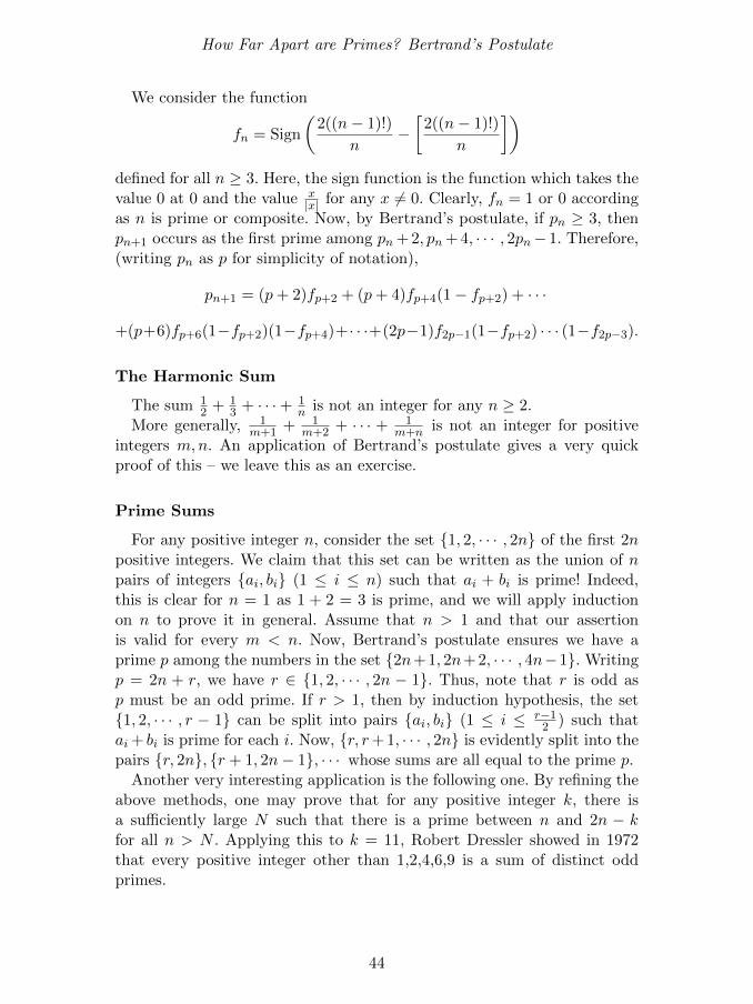
How Far Apart are Primes? Bertrand’s Postulate
We consider the function
fn = Sign
(2((n− 1)!)
n−[
2((n− 1)!)
n
])defined for all n ≥ 3. Here, the sign function is the function which takes thevalue 0 at 0 and the value x
|x| for any x 6= 0. Clearly, fn = 1 or 0 accordingas n is prime or composite. Now, by Bertrand’s postulate, if pn ≥ 3, thenpn+1 occurs as the first prime among pn + 2, pn + 4, · · · , 2pn− 1. Therefore,(writing pn as p for simplicity of notation),
pn+1 = (p+ 2)fp+2 + (p+ 4)fp+4(1− fp+2) + · · ·
+(p+6)fp+6(1−fp+2)(1−fp+4)+· · ·+(2p−1)f2p−1(1−fp+2) · · · (1−f2p−3).
The Harmonic Sum
The sum 12 + 1
3 + · · ·+ 1n is not an integer for any n ≥ 2.
More generally, 1m+1 + 1
m+2 + · · · + 1m+n is not an integer for positive
integers m,n. An application of Bertrand’s postulate gives a very quickproof of this – we leave this as an exercise.
Prime Sums
For any positive integer n, consider the set 1, 2, · · · , 2n of the first 2npositive integers. We claim that this set can be written as the union of npairs of integers ai, bi (1 ≤ i ≤ n) such that ai + bi is prime! Indeed,this is clear for n = 1 as 1 + 2 = 3 is prime, and we will apply inductionon n to prove it in general. Assume that n > 1 and that our assertionis valid for every m < n. Now, Bertrand’s postulate ensures we have aprime p among the numbers in the set 2n+ 1, 2n+ 2, · · · , 4n−1. Writingp = 2n + r, we have r ∈ 1, 2, · · · , 2n − 1. Thus, note that r is odd asp must be an odd prime. If r > 1, then by induction hypothesis, the set1, 2, · · · , r − 1 can be split into pairs ai, bi (1 ≤ i ≤ r−1
2 ) such thatai + bi is prime for each i. Now, r, r+ 1, · · · , 2n is evidently split into thepairs r, 2n, r + 1, 2n− 1, · · · whose sums are all equal to the prime p.
Another very interesting application is the following one. By refining theabove methods, one may prove that for any positive integer k, there isa sufficiently large N such that there is a prime between n and 2n − kfor all n > N . Applying this to k = 11, Robert Dressler showed in 1972that every positive integer other than 1,2,4,6,9 is a sum of distinct oddprimes.
44

How Far Apart are Primes? Bertrand’s Postulate
References
[1] W H Mills, A prime-representing function, Bull. Amer. Math. Soc. 53,pp. 604, 1947.
[2] I Niven and D Zuckermann, Introduction to number theory, John Wileyand Sons, New York, 1960.
[3] S Ramasubramanian, Mathematical Analysis, Echoes from Resonance,Universities Press, Hyderabad, 2001.
[4] T Apostol, Introduction to analytic number theory, Springer Interna-tional Students Edition, Narosa Publishers, New Delhi, 1986.
[5] American Math. Monthly, 1975.
45


Sums of Powers, Bernoulliand the Riemann Zeta function
Bernoulli truly stunned us with his number;woke us up from a deep and ignorant slumber.Its relation with Riemann zetamakes us think nothing could be neater.The connection is much deeper – ask any plumber!
1. Introduction
It is a beautiful discovery due to Jakob Bernoulli that for any positiveinteger k, the sum
∑ni=1 i
k can be evaluated in terms of, what are nowknown as, Bernoulli numbers. It is said that the Bernoulli numbers werediscovered simultaneously and independently by Japanese mathematicianSeki Kowa. Seki Kowa’s discovery was posthumously published in 1712, inhis work Katsuyo Sampo. In this article, we shall discuss several methodsof evaluating the above sum. Apart from Bernoulli’s method which weshall recall, we give a method akin to using integration, and one usingdifferentiation. These methods are often useful in evaluating more generalsums too as we shall indicate. We also discuss connections with the Riemennzeta function – some old and some new.
2. Bernoulli Polynomials and Numbers
To motivate the introduction of the Bernoulli polynomials, let us start
with the sum that we want to evaluate viz.,∑n
i=1 ik. Evidently,
∑ni=1 i
k
k! isthe coefficient of xk in the power series expansion of ex + e2x + · · · + enx.In other words,
e(n+1)x − 1
ex − 1= 1 +
∑k≥0
1k + 2k + · · ·+ nk
k!xk.
Now, the function xex−1 can be represented by a power series x
ex−1 =∑r≥0Br
xr
r! . The numbers Br are known as Bernoulli numbers and it iseasy to evaluate them as follows.
Since the power series x and (ex − 1)∑
r≥0Brxr
r! agree in an intervalaround 0, the numbers are determined recursively as
B0 = 1,∑s<r
(r
s
)Bs = 0 ∀ r ≥ 2.
The chapter is a modified version of an article that first appeared in Resonance, Vol. 8, No. 7,
pp. 54–62, July 2003.
47

Sums of Powers, Bernoulli and the Riemann Zeta function
The first few values are B0 = 1, B1 = −1/2, B2 = 1/6 and B3 = B5 =B7 = · · · = 0.
Now, consider the function Ft(x) = xetx
ex−1 for x 6= 0 and Ft(0) = 1. Once
again, Ft has a power series expansion Ft(x) =∑
k≥0Bk(t)xk
k! .The functions Bk(t) are actually polynomials in t since
∑k≥0
Bk(t)xk
k!= Ft(x) = etx
x
ex − 1= etx
∑k≥0
Bkxk
k!
and thus
Bk(t) =k∑l=0
(k
l
)Blt
k−l.
Bk(t) are called Bernoulli polynomials; note that Bk(0) = Bk.
Returning to our sum, we have that 1k+2k+···+nk
k! is the coefficient of xk ine(n+1)x−1ex−1 i.e., it is the coefficient of xk+1 in x(e(n+1)x−1)
ex−1 = Fn+1(x)−F0(x).
Thus, 1k+2k+···+nk
k! =Bk+1(n+1)−Bk+1
(k+1)! = 1(k+1)!
∑kl=0
(k+1l
)Bl(n+ 1)k+1−l.
In other words,
1k + 2k + · · ·+ nk =1
k + 1
k∑l=0
(k + 1
l
)Bl(n+ 1)k+1−l.
Note that it is evident from this formula that the sum of the k-th powersof the first n natural numbers is a polynomial function of n of degree k+ 1.
3. Method of ‘Integration’
For convenience, let us denote Sk(n) = 1k + 2k + · · · + nk. This is apolynomial function of n i.e., there is a polynomial Sk(x) of degree k + 1such that the above equality holds for all n.
The basic idea of the method we will discuss now is that (since nk = Sk(n)−Sk(n−1)), xk can be thought of as a ‘derivative’ of the function Sk(x). Inother words, Sk(x) itself may be thought of as an ‘integral’ of the functionxk. Of course, this is only heuristic at the moment because xk will be thederivative of Sk at some point between x−1 and x. The correct tool to makethis precise is the ‘method of differences’ which is really a discrete analogueof differentiation. More precisely, let us recall that the ‘backward difference’operator is defined on any function f by (∇f)(x) = f(x)− f(x− 1) for allx. It is trivial to see that if Pr(x) = x(x + 1) · · · (x + r − 1) for r ≥ 1 andfor all x, then (∇Pr)(x) = rPr−1(x) for all x.
48

Sums of Powers, Bernoulli and the Riemann Zeta function
Let us call g an anti-difference of f if ∆g = f . Note that if f is a poly-nomial such that (∇f)(n) = 0 for infinitely many n, then f is a constant.So, if f1, f2 are polynomials with ∇f1 = ∇f2, then f1 − f2 is a constant.
Let us look at our sums Sk(n) now. Let us keep in mind that the polyno-mial Sk(x) has no constant term. Writing fk(x) = xk and gk(x) for any anti-difference of fk which is a polynomial function, then we have (∇gk)(n) =fk(n) = nk = Sk(n)− Sk(n− 1) = (∇Sk)(n) for all n ≥ 2.
Hence, Sk(x) = gk(x)+c for some constant c. Since Sk(x) has no constantterm, we have c = −gk(0).
In other words, Sk(n) = gk(n)−gk(0) for any anti-difference (polynomial)function gk of fk.
Note the similarity with the fundamental theorem of calculus.So, our problem reduces to finding an anti-difference of the function xk.
We observed earlier that the function Pr(x) = x(x+1) · · · (x+r−1) has an
anti-difference Pr+1(x)r+1 . Therefore, it is just a matter of writing xk in terms
of the Pr’s.For instance, k = 1 gives f1(x) = x = P1(x) so that g1(x) can be taken
to be P2(x)2 = x(x+1)
2 so that S1(n) = g1(n)− g1(0) = n(n+1)2 .
For k = 2, one has f2(x) = x2 = x(x+ 1)− x = P2(x)−P1(x) so that g2
can be taken as g2(x) = P3(x)3 − P2(x)
2 = x(x+1)(x+2)3 − x(x+1)
2 = x(x+1)(2x+1)6 .
This gives S2(n) = n(n+1)(2n+1)6 for all n.
The fact that one can indeed write xk as an integer linear combinationof Pk, Pk−1, · · · , P1 can be seen as follows.
Now Pr(x) = x(x + 1) · · · (x + r − 1) = xr + ar−1,rxr−1 + · · · + a0,r for
some integers ai,r. Indeed, these integers are the symmetric polynomials in1, 2, · · · , r − 1.
Then, we have the matrix equation AF = P where A is the upper trian-gular integer matrix
1 ak−1,k ak−2,k · · · a0,k
0 1 ak−2,k−1 · · · a0,k−1
· · ·· · ·
0 0 · · · 0 1,
F is the column vector (xk, xk−1, · · · , x) and, P is the column vector
(Pk(x), Pk−1(x), · · · , P1(x)).The matrix A has an inverse which is also an upper triangular integer
matrix B with 1’s on the diagonal.Thus, F = BP gives the required expression.Let us remark here that the above method is general enough to work
atleast for any complex polynomial function f instead of fk. Thus, to
49

Sums of Powers, Bernoulli and the Riemann Zeta function
evaluate f(1) + · · · + f(n), one writes f as a linear combination of thepolynomials Pr, say,
f(x) = a0 + a1P1(x) + · · ·+ adPd(x)
where d = deg f and ai are complex numbers. Then, one has
f(1) + · · ·+ f(n) = a0n+ a1n(n+ 1)
2+ · · ·+ ad
n(n+ 1) · · · (n+ d)
d+ 1.
4. A Method Involving Differentiation
This is an elementary and pretty useful method involving the differentialoperator x d
dx .
Note that (x ddx)xn = nxn. Therefore, applying it repetitively, one obtains
(x ddx)kxn = nkxn.
Hence 1k + 2k + · · ·+ nk = (x ddx)k(1 + x+ x2 + · · ·+ xn) at x = 1.
This can be rewritten in a more convenient form as
n∑i=1
ik = limx→1(xd
dx)kxn+1 − 1
x− 1.
Riemann Zeta Function
We end with some remarks on the sums of the infinite series∑
n≥11nk
for integers k ≥ 2. This is a special value of the so-called Riemann Zetafunction ζ(s) defined as the sum of the series
∑n≥1
1ns for any real number
s > 1 (actually, it can be defined as a complex valued function for anycomplex number s with Re s > 1 by the same series).
Some of the values are ζ(2) = π2
6 , ζ(4) = π4
90 , ζ(6) = π6
945 .The reader will notice that we have not written ζ(k) for any odd value of
k and that, for even k, the value seems to be a rational multiple of πk. Infact, the value ζ(3) is known to be irrational but it is still unkown if it canbe expressed in terms of ‘known’ constants! We shall show now that ζ(2k)is indeed a rational multiple of π2k for any natural number k. In fact, theBernoulli numbers will surface here again! The reasons for not being ableto evaluate ζ at odd values (or even say whether it is irrational in general)are deep and we do not go into them here.
Now, for any complex number z, we have Sin z = z∏n≥1(1− z2
n2π2 ).Its logarithmic derivative gives us
zCot z = 1 + 2∑n≥1
z2
z2 − n2π2= 1− 2
∑n≥1
∑k≥1
1
n2k
z2k
π2k.
50
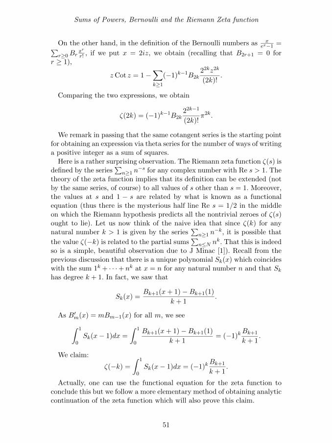
Sums of Powers, Bernoulli and the Riemann Zeta function
On the other hand, in the definition of the Bernoulli numbers as xex−1 =∑
r≥0Brxr
r! , if we put x = 2iz, we obtain (recalling that B2r+1 = 0 forr ≥ 1),
zCot z = 1−∑k≥1
(−1)k−1B2k22kz2k
(2k)!.
Comparing the two expressions, we obtain
ζ(2k) = (−1)k−1B2k22k−1
(2k)!π2k.
We remark in passing that the same cotangent series is the starting pointfor obtaining an expression via theta series for the number of ways of writinga positive integer as a sum of squares.
Here is a rather surprising observation. The Riemann zeta function ζ(s) isdefined by the series
∑n≥1 n
−s for any complex number with Re s > 1. Thetheory of the zeta function implies that its definition can be extended (notby the same series, of course) to all values of s other than s = 1. Moreover,the values at s and 1 − s are related by what is known as a functionalequation (thus there is the mysterious half line Re s = 1/2 in the middleon which the Riemann hypothesis predicts all the nontrivial zeroes of ζ(s)ought to lie). Let us now think of the naive idea that since ζ(k) for anynatural number k > 1 is given by the series
∑n≥1 n
−k, it is possible that
the value ζ(−k) is related to the partial sums∑
n≤N nk. That this is indeed
so is a simple, beautiful observation due to J Minac [1]). Recall from theprevious discussion that there is a unique polynomial Sk(x) which coincideswith the sum 1k + · · ·+ nk at x = n for any natural number n and that Skhas degree k + 1. In fact, we saw that
Sk(x) =Bk+1(x+ 1)−Bk+1(1)
k + 1.
As B′m(x) = mBm−1(x) for all m, we see∫ 1
0Sk(x− 1)dx =
∫ 1
0
Bk+1(x+ 1)−Bk+1(1)
k + 1= (−1)k
Bk+1
k + 1.
We claim:
ζ(−k) =
∫ 1
0Sk(x− 1)dx = (−1)k
Bk+1
k + 1.
Actually, one can use the functional equation for the zeta function toconclude this but we follow a more elementary method of obtaining analyticcontinuation of the zeta function which will also prove this claim.
51

Sums of Powers, Bernoulli and the Riemann Zeta function
The analytic continuation of the zeta function to all s 6= 1 and thefact that lims→1(s − 1)ζ(s) = 1 are obtainable as follows. Now, the zetafunction ζ(s) is defined for a complex variable s by the series
∑∞n=1 n
−s
which converges for Re s) > 1. We shall use Abel’s partial summationformula which is an elementary yet very powerful formula – the readers arewell aware of its continuous analogue – integration by parts.
If an, bn are two sequences of complex numbers, and if An = a1 +· · ·+ an, then we have the identity
a1b1 + · · ·+ anbn = Anbn+1 −n∑k=1
Ak(bk+1 − bk).
Thus,∑
n anbn converges if both the sequence Anbn+1 and the series∑∞k=1Ak(bk+1 − bk) converge.
The proof follows simply by observing that
n∑k=1
akbk =n∑k=1
(Ak −Ak−1)bk −n∑k=1
Akbk −n∑k=1
Akbk+1 +Anbn+1.
In our case, by using Abel’s partial summation formula, one has
ζ(s) = s
∫ ∞1
[x]
xs+1dx =
s
s− 1− s
∫ ∞1
xxs+1
dx.
Here [x] and x respectively denote the integral part and the fractionalpart of x. Note that the integral converges for Re (s) > 0 and thus the lastexpression gives the analytic continuation of the zeta function to the regionRe (s) > 0. We shall proceed inductively now. On writing∫ ∞
1
xxs+1
dx =∞∑n=1
∫ n+1
n
x− nxs+1
=∞∑n=1
∫ 1
0
udu
(u+ n)s+1
and integrating the last integral by parts, we obtain
ζ(s) =s
s− 1− s
2(ζ(s+ 1)− 1)− s(s+ 1)
2
∫ ∞1
x2
xs+2dx.
From this, we have analytic continuation of ζ for Re (s) > −1 and alsothat ζ(0) = −1
2 . Proceeding inductively, we get
ζ(s) = 1 +1
s− 1−
m∑q=1
s(s+ 1) · · · (s+ q − 1)
(q + 1)!(ζ(s+ q)− 1)
−s(s+ 1) · · · (s+m)
(m+ 1)!
∞∑n=1
∫ 1
0
um+1
(u+ n)s+m+1.
52

Sums of Powers, Bernoulli and the Riemann Zeta function
The infinite sum on the right hand side converges for Re (s) > −m andthus we have an expression for ζ(s) for such s. At this point, we evaluateit at s = 1 −m. Rather surprisingly, this pretty but simple idea does notseem to have been thought of until very recently when it was done so byRam Murty and M Reece. We get
ζ(1−m) = 1− 1
m+
(−1)m
m(m+ 1)−m−1∑q=1
(−1)q(m− 1
q
)1
q + 1(ζ(1−m+q)−1).
The first few values at nonpositive integers are
ζ(0) = −1
2, ζ(−1) = − 1
12, ζ(−2) = 0, ζ(−3) =
1
120.
On the other hand, for M = 1, 2, 3, · · · , we have
Mk+1 =
k∑r=0
(k + 1
r + 1
)(−1)rSk−r(M − 1).
Therefore, we get
k∑r=0
(k + 1
r + 1
)(−1)r
∫ 1
0Sk−r(x− 1)dx =
(−1)k+1
k + 2.
As ζ(0) = −12 , we arrive at the formula
ζ(−k) =
∫ 1
0Sk(x− 1)dx = (−1)k
Bk+1
k + 1
which was claimed.Let us finally remark that the Riemann zeta function vanishes at the
negative even integers −2,−4,−6, · · · and these are its so-called trivialzeroes. The Riemann hypothesis asserts that all other zeroes lie on the lineRe(s) = 1/2.
References
[1] J Minac, Expo. Math., Vol. 12, pp. 459–462, 1994.
53


Frobenius and His Density Theoremfor Primes
A rare sight is seen; yes,when we spot a genius.We saw one who made senseof prime numbers being dense.This was the great George Frobenius!
1. Introduction
Our starting point is the following problem which appeared in the recentIMO (International Mathematical Olympiad):
If p is a prime number, show that there is another prime number q suchthat np − p is not a multiple of q for any natural number n.
Now, this problem itself can be solved using elementary mathematics(otherwise, it would not be posed in the IMO). However, how does oneguess that such a thing ought to be true? Can we produce an abundance ofsuch problems in some systematic manner? We take this problem as a pointof reference to discuss some deep number theory (which is already a centuryold) which not only solves this problem, but also gives us an understandingof why such facts are true and what more one can expect. The main theoremunder discussion is known as Frobenius’s density theorem.
2. Rephrasing and Generalisation
Let us start by rephrasing the above problem. For a prime p, consider theintegral polynomial f(X) = Xp−p. For any prime q, one may consider f asa polynomial over Z/qZ, the integers modulo q by reducing the coefficientsof f modulo q. Then, the problem asks us to prove that there is some primeq for which f does not have a root in Z/qZ. So, when is it true that anintegral polynomial has roots in Z/qZ for every prime p? Obviously, if theintegral polynomial already has an integral root, this happens. Can it alsohappen when f has no integral root?
Before answering this, let us note that every nonconstant integral poly-nomial has a root in Z/qZ for infinitely many primes q. Here is the simpleargument proving it. See also ‘Polynomials with integer values’, secondchapter in this book.
The chapter is a modified version of an article that first appeared in Resonance, Vol. 8, No. 12,
pp. 33–41, December 2003.
55

Frobenius and His Density Theorem for Primes
Let P (X) = a0 +a1X+ · · ·+anXn be an integral polynomial with n > 0
and an 6= 0. For any integer d, look at the polynomial
P (a0dX) = a0(1 + a1dX + a0a2d2X2 + · · ·+ an−1
0 andnXn).
Since Q(X) = 1+a1dX+a0a2d2X2 + · · ·+an−1
0 andnXn takes the values
0, 1,−1 at the most for finitely many values of X, it takes a value Q(m)6= 0, 1,−1 which must then be a multiple of some prime p. As Q(m) ≡ 1mod d, p is coprime to d. Therefore, for any d, we have shown that thereis some m such that P (a0dm) is zero modulo p for some prime p coprimeto d. Varying d, we have infinitely many such primes p.
The set of odd primes modulo which the polynomial X2 + 1 has roots,consists precisely of all primes in the arithmetic progression 4n + 1. Ingeneral, every quadratic polynomial has a corresponding arithmetic pro-gression such that the polynomial has roots modulo each prime in thisprogression, and modulo no other primes. This follows from the famousquadratic reciprocity law.
Returning to our case f(X) = Xp−p, let us see whether we can explicitlyget an infinite set of primes modulo which f does have roots. Considerany prime q and the group (Z/qZ)∗ of nonzero integers modulo q undermultiplication modulo q. If the p-th power map θ : a 7→ ap on (Z/qZ)∗ isnot 1 − 1, then there exists some a 6= 1 with ap = 1. Since aq−1 = 1, wemust have p
(q− 1) . In other words, whenever q 6≡ 1 mod p, our polynomial fhas a root modulo q.
Let us now return to the possibility of producing a polynomial whichhas no integral roots but has roots modulo every integer. Consider thepolynomial
g(X) = (X2 − 13)(X2 − 17)(X2 − 221).
Evidently, its roots ±√
13,±√
17,±√
221 are not integral (or even ratio-nal). We show that it has roots modulo any nonzero integer. Recall that theChinese remainder theorem tells us that whenever m1, · · · ,mr are pairwisecoprime integers and a1, · · · , ar are any integers, there is an integer a whichis simultaneously ≡ ai mod mi for i = 1, · · · , r. Therefore, by the Chineseremainder theorem, it suffices to prove that g has roots modulo every primepower. In what follows, for any prime p and a coprime to p, the notation(ap ) stands for 1 or −1 according as whether a is a square or not mod p.One also says in the respective cases that a is a quadratic residue modulop and a is a quadratic nonresidue modulo p.
Let us look at g now. If p is an odd prime such that (13p ) = 1, then
t2 ≡ 13 mod p for some integer t. We show by induction on n that x2 ≡ 13mod pn has a solution. Suppose t2 ≡ 13 mod pn−1, say t2 = 13 + upn−1.Consider t0 = t+ pn−1t1 where we shall choose t1 so that t20 ≡ 13 mod pn.
56
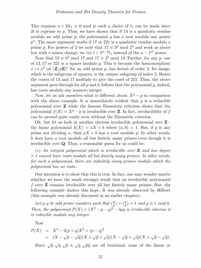
Frobenius and His Density Theorem for Primes
This requires u + 2tt1 ≡ 0 mod p; such a choice of t1 can be made since2t is coprime to p. Thus, we have shown that if 13 is a quadratic residuemodulo an odd prime p, the polynomial g has a root modulo any powerpn. The same argument works if 17 or 221 is a quadratic residue modulo aprime p. For powers of 2 we note that 17 ≡ 32 mod 23 and work as abovebut with a minor change; we try t+ 2n−2t1 instead of the n− 1st power.
Note that 13 ≡ 82 mod 17 and 17 ≡ 22 mod 13. Further, for any p, oneof 13, 17 or 221 is a square modulo p. This is because the homomorphismx 7→ x2 on (Z/pZ)∗ for an odd prime p, has kernel of order 2. Its image,which is the subgroup of squares, is the unique subgroup of index 2. Hencethe cosets of 13 and 17 multiply to give the coset of 221. Thus, the aboveargument goes through for all p and it follows that the polynomial g, indeed,has roots modulo any nonzero integer.
Now, let us ask ourselves what is different about Xp − p in comparisonwith the above example. It is immediately evident that g is a reduciblepolynomial over Z while the famous Eisenstein criterion shows that thepolynomial f(X) = Xp− p is irreducible over Z. In fact, irreducibility of fcan be proved quite easily even without the Eisenstein criterion.
Ok, but let us look at another obvious irreducible polynomial over Z -the linear polynomial h(X) = aX + b where (a, b) = 1. But, if p is anyprime not dividing a, then aX + b has a root modulo p. In other words,h does have a root modulo all but finitely many primes even though it isirreducible over Q. Thus, a reasonable guess for us could be:
(∗) An integral polynomial which is irreducible over Z and has degree> 1 cannot have roots modulo all but finitely many primes. In other words,for such a polynomial, there are infinitely many primes modulo which thepolynomial has no roots.
Our intention is to show that this is true. In fact, one may wonder maybewhether we have the much stronger result that an irreducible polynomialf over Z remains irreducible over all but finitely many primes. But, thefollowing example dashes this hope. It was already observed by Hilbert(this example was already discussed in an earlier chapter).
Let p, q be odd prime numbers such that (pq ) = ( qp) = 1 and p ≡ 1 mod 8.
Then, the polynomial P (X) = (X2 − p− q)2 − 4pq is irreducible whereas itis reducible modulo any integer.
Now
P (X) = X4 − 2(p+ q)X2 + (p− q)2
= (X −√p−√q)(X +√p+√q)(X −√p+
√q)(X +
√p−√q).
Since√p,√q,√p ± √q,√pq are all irrational, none of the linear or
57

Frobenius and His Density Theorem for Primes
quadratic factors of P (X) are in Z[X] i.e. P (X) is irreducible over Z.Note, as before, that it is enough to show that a factorisation of P existsmodulo any prime power as we can use Chinese reminder theorem to geta factorisation modulo a general integer. Now, P (X) can be written in thefollowing ways:
P (X) = X4 − 2(p+ q)X2 + (p− q)2
= (X2 + p− q)2 − 4pX2
= (X2 − p+ q)2 − 4qX2
= (X2 − p− q)2 − 4pq.
The second and third equalities above show that P (X) is reducible mod-ulo any qn and any pn respectively. Also since p ≡ 1 mod 8, p is a quadraticresidue modulo 2 and, therefore, modulo any 2n; the second equality aboveagain shows that P (X) is the difference of two squares modulo 2n, andhence reducible mod 2n.
If ` is a prime 6= 2, p, q, at least one of (p` ), ( q` ) and (pq` ) is 1 by the productformula (p` ) · ( q` ) · (pq` ) = 1 that we noted earlier. According as (p` ), ( q` ) or(pq` ) = 1, the second, third or fourth equality shows that P (X) is reduciblemod `n for any n.
We mention, in passing, a very simple but important general method ofproving the irreducibility of an integral polynomial. This will also set upthe notation for our main statement when we address (∗). To illustrate it,consider the polynomial p(X) = X4 + 3X2 + 7X + 4. Modulo 2, we havep(X) = X(X3 + X + 1) and both factors are irreducible over the fieldZ/2Z. We say that the decomposition type of p(X) mod 2 is 1, 3. Therefore,either p is irreducible over Z or if not, it is a product of a linear factorand an irreducible factor of degree 3 over Z. But, modulo 11, we havep(X) = (X2 + 5X − 1)(X2 − 5X − 4) where both factors are irreducibleover the field Z/11Z. That is, the decomposition type of p mod 11 is 2, 2.Thus, it cannot be that p has a linear factor over Z. In other words, p mustbe irreducible over Z.
3. The Notion of Density of Primes
Let us get back to the guess quoted above as (∗). We need some notations.Let f be a monic integral polynomial of degree n. Suppose that f has dis-tinct roots α1, · · · , αn ∈ C; equivalently, the discriminant disc(f) 6= 0. LetK = Q(α1, · · · , αn), the subfield of C generated by the roots; that is, allrational expressions in the αi’s with coefficients from Q. This is the smallestsubfield of C which contains all the αi’s; it is also known as the splitting fieldof f for the reason that f splits into the product
∏ni=1(X−αi) over K. We
58

Frobenius and His Density Theorem for Primes
look at the group G of those permutations of αi’s which give rise to a fieldautomorphism of K. This is known as the Galois group of f and denotedby Gal(f). For instance, if f(X) = X2 − a for some nonsquare integer a,then K = Q(
√a) where
√a denotes a square root of a in C and G has two
elements I, σ where σ interchanges√a and −
√a. In general, although G is
a subgroup of Sn, the permutations which belong to G are rather restricted;for example if f is irreducible over Q, then a permutation in G is neces-sarily transitive on the αi’s. If p 6 |disc(f), then the decomposition type off modulo p gives a partition of n as we saw above. On the other hand,each element of G has a cycle decomposition as an element of Sn and, thusdefines a partition of n as well. Frobenius’s wonderful idea is to relate thenumbers of such partitions for a particular type. This will be expressed interms of a notion of density of a set of prime numbers.
A set S of primes is said to have density δ if∑
p∈S 1/p∑all p 1/p → δ as s → 1+.
Here 1+ means the limit when s tends to 1 from the right. For instance,any finite set of primes has density 0. Using this notion of density, we statemore precisely:
4. Frobenius Density Theorem
The set of primes p modulo which a monic integral, irreducible polyno-mial f has a given decomposition type n1, n2, · · · , nr, has density equal toN/O(Gal(f)) where N = |σ ∈ Gal(f) : σ has a cycle pattern n1, n2, · · · , nr|.
As we point out now, our guess (∗) is vindicated by this theorem and alittle bit of group theory; in particular, this also solves the IMO problem.
If f is irreducible, and has roots modulo all but finitely many primes,then the theorem shows that each σ has a cycle pattern of the form 1, n2, · · ·This means that each element of Gal(f) fixes a root. Since the roots of fare transitively moved around by Gal(f), this group would be the union ofthe conjugates of its subgroup H consisting of elements which fix a root off , say α1. However, it is an elementary exercise that a finite group cannotbe the union of conjugates of a proper subgroup. Thus, in our case H =Gal(f). This means that Gal(f) fixes each αi and is therefore trivial. Thatis, f is linear.
A famous theorem of Dirichlet on primes in arithmetic progressions as-serts that the density of the set of primes p ≡ a mod n is 1/φ(n) for any(a, n) = 1. Dirichlet’s theorem implies Frobenius’s theorem for the polyno-mial f(X) = Xn−1. The converse conclusion cannot quite be made. Thus,Frobenius formulated a conjecture which generalises both his theorem andDirichlet’s theorem. This was proved 42 years later by Chebotarev and isknown now as the Chebotarev density theorem. This is an extremely usefulresult and even effective versions are known (see the end of the article for
59

Frobenius and His Density Theorem for Primes
what the word ‘effective’ means here). Chebotarev’s idea of proving thishas been described by two prominent mathematicians as “a spark fromheaven”. In fact, this theorem was proved in 1922 (“while carrying waterfrom the lower part of town to the higher part, or buckets of cabbages tothe market, which my mother sold to feed the entire family”) and EmilArtin wrote to Hasse in 1925: “Did you read Chebotarev’s paper? ... Ifit is correct, then one surely has the general abelian reciprocity laws inone’s pocket...” Artin found the proof of the general reciprocity law in 1927using Chebotarev’s technique (he had already boldly published the reci-procity law in 1923 but admitted that he had no proof). Nowadays, Artin’sreciprocity law is proved in some other way and Chebotarev’s theorem isdeduced from it!
To state Chebotarev’s theorem, we recall one notion – the Frobeniusmap. The idea is that given a monic integral polynomial f and its split-ting field K, we can associate to any prime p 6 |disc(f), an element Φp
of Gal(f) in a natural manner. If we can do this, one may expect thatthe decomposition type of f modulo p coincides with the cycle patternof Φp. It can almost be done except that a prime p gives rise to a con-jugacy class of elements in Gal(f). We do not define the Frobenius con-jugacy class here as it is somewhat technical and merely explain someproperties it has. For any prime number p, the p-th power map Frobpis an automorphism of the field Fp which is identity on Fp. Therefore,Frobp permutes the roots of any polynomial over Fp. Indeed, the Ga-lois theory of finite fields amounts to the statement that if g is a poly-nomial over Fp with simple roots, then the cycle pattern of Frobp viewedas a permutation of the roots of g coincides with the decomposition typeof g over Fp. In our case, we start with an integral polynomial f andlook at it modulo p for various primes p. The basic theory of algebraicnumbers shows that whenever p 6 |disc(f), the automorphism Frobp givesrise to a conjugacy class in Gal(f), called the Frobenius conjugacy classmodulo p.
In Frobenius’s density theorem, one cannot distinguish between two primesp, q defining different conjugacy classes C(x) and C(y) but some powers ofx and y are conjugate. For instance, for the polynomial X10−1, the decom-position type modulo primes congruent to 1, 3, 7, 9 mod 10 are, respectively,1, 1, 1, 1, 1, 1, 1, 1, 1, 1; 1, 1, 4, 4; 1, 1, 4, 4; 1, 1, 2, 2, 2, 2.
Frobenius’s theorem cannot distinguish between primes which are 3 mod10 and those which are 7 mod 10; they define different conjugacy classesin Gal(X10 − 1). Thus, it would imply that the number of primes ≡ 3 or 7mod 10 is infinite but doesn’t say whether each congruence class containsinfinitely many primes. This is what Chebotarev’s theorem asserts.
60
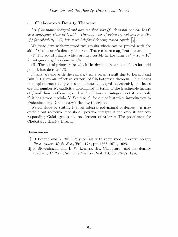
Frobenius and His Density Theorem for Primes
5. Chebotarev’s Density Theorem
Let f be monic integral and assume that disc (f) does not vanish. Let Cbe a conjugacy class of Gal(f). Then, the set of primes p not dividing disc
(f) for which σp ∈ C, has a well-defined density which equals |C||G| .
We state here without proof two results which can be proved with theaid of Chebotarev’s density theorem. These concrete applications are:
(I) The set of primes which are expressible in the form 3x2 + xy + 4y2
for integers x, y, has density 1/5.(II) The set of primes p for which the decimal expansion of 1/p has odd
period, has density 1/3.Finally, we end with the remark that a recent result due to Berend and
Bilu [1]) gives an ‘effective version’ of Chebotarev’s theorem. This meansin simple terms that given a nonconstant integral polynomial, one has acertain number N , explicitly determined in terms of the irreducible factorsof f and their coefficients, so that f will have an integral root if, and onlyif, it has a root modulo N . See also [2] for a nice historical introduction toFrobenius’s and Chebotarev’s density theorems.
We conclude by stating that an integral polynomial of degree n is irre-ducible but reducible modulo all positive integers if and only if, the cor-responding Galois group has no element of order n. The proof uses theChebotarev density theorem.
References
[1] D Berend and Y Bilu, Polynomials with roots modulo every integer,Proc. Amer. Math. Soc., Vol. 124, pp. 1663–1671, 1996.
[2] P Stevenhagen and H W Lenstra, Jr., Chebotarev and his densitytheorem, Mathematical Intelligencer, Vol. 18, pp. 26–37, 1996.
61


When is a Decimal ExpansionIrrational?
Everyone learns in school that√
2 is irrational. This, along with Euclid’sproof of infinitude of primes, is probably the first time she encounters aproof by contradiction. Most students know in school that the value of
√2
is approximately 1.414 but, more often than not, this aspect is not pursuedfurther in detail. The decimal 0.999 · · · where 9 recurs indefinitely is under-stood (after some persuasion perhaps) to be none else than the number 1.The problem here is that the concept of limit takes some time to sink in.Given that start, they can see easily that numbers like 0.142857 wherethe digits overlined recur indefinitely, are rational. Even if the recurringstring occurs after an initial string (for example, a decimal expansion like27.142857), it still gives us a rational value only because it is the sum of ageometric series with a ratio of the form 10k.
It is not hard to prove that this is a necessary condition as well, thatis, a decimal expansion of a real number represents a rational number if,and only if, after the decimal place, there is a finite (possibly empty) stringafter which the digits consist of a finite string (possibly consisting entirelyof zeroes) recurring indefinitely.
Thus, for instance, the number 0.101001000 · · · where the number ofzeroes keeps increasing by 1 has to represent an irrational number. However,from the decimal expansion, sometimes it is not clear whether there is suchan eventual recurrence or not. This could be due to our present state ofknowledge. For instance, one could define a number 0.1010 · · · where thenumber of zeroes occurring at the n-th step is either increased by one orkept the same according as to whether the number 22n + 1 is prime or not.Since one does not know whether there are infinitely many such primes, wecannot say at present as to whether the above decimal represents a rationalor an irrational number.
The decimal 0.1234 · · · , where the natural numbers are written in se-quence, is clearly irrational since, for instance, the number of zeroes occur-ring in the powers of 10 keeps increasing. The decimal 0.235711 · · · , wherethe set of primes is written down in sequence, is also irrational. This isbecause there is a prime of the form 10na + 1 for an arbitrary n – thiswas proved in an earlier chapter. Here is another elementary general result(see [1]).
The chapter is a modified version of an article that first appeared in Resonance, Vol. 9, No. 3,
pp. 78–80, March 2004.
63
When is a Decimal Expansion Irrational?
Consider a decimal x = 0.a1a2 · · · where an is a strictly increasingsequence of natural numbers having the property that
∑n
nr
asndiverges for
some r, s > 0. Then x is irrational.
Note that since the reciprocals of primes do not sum to a finite quantity,this result also implies that 0.23571113 · · · is irrational.
To prove this, assume, if possible, that x is rational. Then, by throwingout some of the first a’s and scaling, we may assume that the decimal isactually periodic and not just eventually periodic. Let t denote a period.Let N1 < N2 < · · · denote the natural numbers representing the differentnumbers of digits occurring for the ai’s. Let di denote the number of ai’swhich have exactly Ni digits. In other words, a1, · · · , ad1 are the a’s withN1 digits and, for each i ≥ 1, the numbers
ad1+···+di+1, · · · , ad1+···+di+di+1
are the a’s which have exactly Ni+1 digits. Let us write for simplicity d0 = 0.Now, if some di+1 were bigger than t, then the numbers
ad1+···+di+1, · · · , ad1+···+di+t+1,
would all have Ni+1 digits and since the length of the string
(ad1+···+di+1) · · · (ad1+···+di+t),
is tNi+1 which is a multiple of t, it follows that
ad1+···+di+1 = ad1+···+di+t+1,
which is a manifest contradiction of the assumption that an is an increas-ing sequence. Hence, we have shown that each di is ≤ t.
Now, we also have the evident inequalities
ad1+···+di+di+1≥ · · · ≥ ad1+···+di+1 ≥ 10Ni+1−1,
since these numbers have Ni+1 digits. We shall show that∑∞
n=1nr
asncon-
verges. Now, for each i ≥ 0,
d1+···+di+di+1∑j=d1+···+di+1
jr
asj≤
d1+···+di+di+1∑j=d1+···+di+1
(d1 + · · ·+ di+1)r
10s(Ni+1−1)≤ di+1(d1 + · · ·+ di+1)r
10s(Ni+1−1).
Thus,∑
i≥0
∑d1+···+di+di+1
j=d1+···+di+1jr
asj≤
∑i≥0
t(i+1)rtr
10s(Ni+1−1) ≤ tr+1
10s(N1−1)
∑i≥0
(i+1)r
10is.
But, the last series converges so that∑∞
n=1nr
asnalso converges. This is a
contradiction of our assumption and the irrationality of x follows.
References
[1] A McD Mercer, American Mathematical Monthly, Vol. 101,pp. 567–568, 1994.
64

Revisiting Kummer’sand Legendre’s Formulae
In a beginning course in number theory, an elementary exercise is tocompute the largest power of a prime p dividing n!. This number, calledthe p-adic valuation of n!, is easily proved to be
vp (n!) =
[n
p
]+
[n
p2
]+
[n
p3
]+ · · · . (1)
Note that this is a finite series. The number vp(n!) comes up naturallyin a few situations like the following. In the group of permutations of nobjects, this would give the power of p which is the order of a p-Sylowsubgroup. While discussing p-adic numbers as analogues of the usual realnumbers, one looks at the analogue of the exponential series. The expressionfor vp(n!) leads one to determine that the exponential series has the radiusof convergence p−1/(p−1).
Now, vp(n!) can also be computed in another manner by a beautiful ob-servation due to the legendary mathematician Legendre. Legendre observedthat the p-adic valuation of n! can be read off from the base-p expansionof n. It is simply n−s(n)
p−1 where s(n) is the sum of the “digits” of n in thisexpansion. A related result that Kummer proved is that, if r ≤ n, thenthe p-adic valuation of the binomial coefficient
(nr
)is simply the number
of ‘carry-overs’ when one adds r and n − r in base-p. In ([1], pp.229–233)Honsberger deduces Kummer’s theorem from Legendre’s result and refersto Ribenboim’s lovely book [2], pp.30–32) for a proof of the latter. Riben-boim’s proof is by verifying that Legendre’s base-p formula agrees with thestandard formula (1).
Is it possible to prove Legendre’s formula without recourse to the aboveformula? We shall see that this is indeed possible and that the standardformula above follows from such a proof. What is more, Kummer’s formulaalso follows without having to use Legendre’s result. Let us start by recallingLegendre’s formula.
Legendre’s Formula
Let p be a prime number and let ak · · · a1a0 be the base-p expansion ofa natural number n. We shall show that if Legendre’s formula
vp (n!) =n− s(n)
p− 1=
n−∑k
i=0 aip− 1
(2)
The chapter is a modified version of an article that first appeared in Resonance, Vol. 10, No. 2,
pp. 62–71, February 2005.
65
Revisiting Kummer’s and Legendre’s Formulae
holds good for n, then it also holds good for pn+ r for any 0 ≤ r < p. Notethat the base-p expansion of pn + r is
ak · · · a1a0 r.
Let us denote, for convenience, the number m−s(m)p−1 by f(m) for any
natural number m. Evidently,
f(pn + r) =pn−
∑ki=0 ai
p− 1= n + f(n).
On the other hand, it follows by induction on n that
vp ((pn + r)!) = n + vp(n!). (3)
For, if it holds good for all n < m, then
vp((pm + r)!) = vp(pm) + vp((pm− p)!)
= 1 + vp(m) + m− 1 + vp((m− 1)!) = m + vp(m!).
Since it is evident that f(m) = 0 = vp(m!) for all m < p, it follows thatf(n) = vp(n!) for all n. This proves Legendre’s formula.
Note also that the formula
vp(n!) =
[n
p
]+
[n
p2
]+
[n
p3
]+ · · ·
follows inductively on using (3).
Kummer’s Algorithm
As before p is any prime number. For any natural numbers r and s, letus denote by g(r, s) the number of ‘carry-overs’ when the base-p expansionsof r and s are added. Kummer’s result is that for k ≤ n,
vp
((n
k
))= g(k, n− k). (4)
Once again, this is clear if n < p, as both sides are then zero. We shallshow that if the formula holds good for n (and every k ≤ n), it does so forpn + r for 0 ≤ r < p (and any k ≤ pn + r). This would prove the result forall natural numbers.
Consider any binomial coefficient(pn+rpm+a
)for 0 ≤ a < p.
First, suppose a ≤ r.
66

Revisiting Kummer’s and Legendre’s Formulae
Write m = bk · · · b0 and n − m = ck · · · c0 in base-p. Then the base-pexpansions of pm + a and p(n−m) + (r − a) are, respectively,
pm + a = bk · · · b0 a
p(n−m) + (r − a) = ck · · · c0 r − a.
Evidently, the corresponding number of carry-overs is
f(pm + a, p(n−m) + (r − a)) = f(m,n−m).
By the induction hypothesis, f(m,n−m) = vp((nm
)). Now vp
((pn + r
pm + a
))is equal to
vp((pn + r)!)− vp((pm + a)!)− vp((p(n−m) + r − a)!)
= n + vp(n!)−m− vp(m!)− (n−m)− vp((n−m)!) = vp
((n
m
)).
Thus, we are through in the case when a ≤ r.
Now suppose that r < a. Then vp
((pn + r
pm + a
))is equal to
vp((pn + r)!)− vp((pm + a)!)− vp((p(n−m− 1) + (p + r − a))!)
= n + vp(n!)−m− vp(m!)− (n−m− 1)− vp((n−m− 1)!)
= 1 + vp(n) + vp((n− 1)!)− vp(m!)− vp((n−m− 1)!)
= 1 + vp(n) + vp
((n− 1
m
)).
We need to show that
f(pm + a, p(n−m− 1) + (p + r− a)) = 1 + vp(n) + f(m,n−m− 1). (5)
Note that m < n. Write n = ak · · · a0, m = bk · · · b0 and n − m − 1 =ck · · · c0 in base-p. If vp(n) = d, then ai = 0 for i < d and ad 6= 0. In base-p,we have
n = ak · · · ad 0 · · · 0
and, therefore,
n− 1 = ak · · · ad+1ad − 1 p− 1 · · · p− 1.
Now, the addition m+ (n−m− 1) = n− 1 gives bi + ci = p− 1 for i < d(since they must be < 2p− 1). Moreover, bd + cd = ad − 1 or p + ad − 1.
67

Revisiting Kummer’s and Legendre’s Formulae
Note the base-p expansions
pm + a = bk · · · b0 a,
p(n−m− 1) + (p + r − a) = ck · · · c0 p + r − a.
We add these using that fact that there is a carry-over in the beginningand that 1 + bi + ci = p for i < d. Since there is a carry-over at the firststep as well as at the next d steps, we have
pn + r = ∗ ∗ · · · ad 0 · · · 0 r
where there are d zeroes before r, and
f(pm + a, p(n−m− 1) + (p + r − a)) = 1 + d + f(m,n−m− 1).
This proves Kummer’s assertion also.We end with the remark that Kummer’s result gives an immediate proof
of the fact that the n-th Catalan number is odd if and only if n is 1 lessthan a power of 2.
References
[1] R Honsberger, In Polya’s Footsteps, published and distributed by theMathematical Association of America, 1997.
[2] P Ribenboim, The Book of Prime Number Records, Springer-Verlag,1996.
68
Bessels Contain Continued Fractionsof Progressions
1. Introduction
The January 2000 issue of Resonance carried a nice article on continuedfractions by Shailesh Shirali. After discussing various continued fractionsfor numbers related to e, he left us with the intriguing question as to howone could possibly evaluate the continued fraction
1
1+
1
2+
1
3+· · · · · · · · · .
The question is interesting because this continued fraction is simpler-looking than the ones which were studied in that article. We answer thisquestion here and show that the discussion naturally involves the Besselfunctions, thus explaining the title. However, we shall begin with somedetails about continued fractions which complement his discussion. Oneplace where continued fractions are known to appear naturally is in thestudy of the so-erroneously-called Pell’s equation.
In a series of very interesting articles in Resonance, Amartya KumarDutta had discussed various aspects of Mathematics in ancient India. Inparticular, he discussed Brahmagupta’s and Bhaskara’s work on Samasab-havana and the Chakravala method for finding solutions to ‘Pell’s equation’.In fact, it is amusing to recall what Andre Weil, one of the great mathe-maticians of the last century wrote once, while discussing Fermat’s writingson the problem of finding integer solutions to x2 −Dy2 = 1:
What would have been Fermat’s astonishment if some mission-ary, just back from India, had told him that his problem hadbeen successfully tackled there by native mathematicians almostsix centuries earlier!
The Chakravala method can be described in terms of continued fractions.Let us begin with some rather elementary things which were known so longback and have gone out of fashion to such an extent that they are not aswidely known as they ought perhaps to be.
The chapter is a modified version of an article that first appeared in Resonance, Vol. 10, No. 3,pp. 80–87, March 2005.
69
Bessels Contain Continued Fractions of Progressions
2. Linear Diophantine Equations with SCF’s
Let us denote by[a0 ; a1, a2, a3, · · · ] (1)
the SCF (simple continued fraction)
a0 +1
a1+
1
a2+· · · · · · . (2)
Here the ai are natural numbers. Evidently, any rational number has afinite SCF. For instance,
763
396= [1 ; 1, 12, 1, 1, 1, 9].
Its successive convergents are 11 ,
21 ,
2513 ,
2714 ,
5227 ,
7941 ,
763396 . Note that if the n-
th convergent is pnqn
, then pnqn−1 − pn−1qn = (−1)n. This holds for anycontinued fraction, as can be seen by induction. This gives a method offinding all positive integral solutions (in particular, the smallest one) x, yto a Diophantine equation of the form ax − by = c. For instance, considerthe equation
396x− 763y = 12.
Look at the SCF for 763396 and compute its penultimate convergent 79
41 .Now, if x, y are positive integers satisfying
396x− 763y = 12,
then combining with the fact that 396× 79− 763× 41 = 1, we get
x− (79× 12) = 763t, y − (41× 12) = 396t
for some integer t. This gives all solutions, and the smallest solution innatural numbers x, y is obtained by taking t = −1 and turns out to be(185, 96).
The reader is left with deriving similarly the corresponding expressionfor any linear equation.
3. Quadratic Equations from SCF’s
Evidently, finite CF’s give only rational numbers. Given the fact thata periodic decimal expansion gives rational numbers too, a reader mightbe tempted to guess that a periodic CF gives rationals. After just a lit-tle thought, it becomes apparent that an eventually periodic SCF gives aquadratic irrational number. For example, [1 ; 1, 1, · · · ] is the ‘golden ratio’
70

Bessels Contain Continued Fractions of Progressions
(1 +√
5)/2. This is because the value s satisfies s = 1 + 1/s and is posi-tive. Similarly, the SCF [1 ; 3, 2, 3, 2, · · · ] =
√5/3, as it gives the quadratic
equation s− 1 = (s+ 1)/(3s+ 4), and [0 ; 3, 2, 1, 3, 2, 1, · · · ] = (√
37− 4)/7as it gives the equation s = (3 + 2s)/(10 + 7s), etc.
Consider a quadratic Diophantine equation in two variables
ax2 + 2hxy + by2 + 2gx+ 2fy + c = 0 (3)
where a, b, c, f, g, h are integers. Thinking of this as a polynomial in x andsolving it, one obtains
ax+ hy + g = ±√
(h2 − ab)y2 + 2(hg − af)y + g2 − ac).
For any integral solution, the expression inside the square root (which wewrite as ry2 + 2sy + t now) must be a perfect square, say v2. Once again,solving this as a polynomial in y, we get
ry + s = ±√
(s2 − rt+ rv2).
Hence, s2−rt+rv2 must be a perfect square u2. In other words, the origi-nal equation does not have integral solutions unless the equation u2−rv2 =w has a solution, where w is a constant defined in terms of a, b, c, f, g, h.
An equation of the form u2 + rv2 = w for r positive has only finitelymany solutions. Therefore, let us discuss the equation u2 − rv2 = ±wwhere r, w are positive integers and r is not a perfect square. The SCFfor√r provides a way of obtaining infinitely many solutions of the special
equation u2 − rv2 = 1. Consequently, for given r, w if we find one solution(u0, v0) of u2−rv2 = w, one can find infinitely many by the samasabhavana(composition) x = uu0 + rvv0, y = uv0 + vu0 for any u, v with u2 − rv2 =1. However, the method of CF’s will provide even one solution only forcertain w’s; namely, those which appear as one of the denominators whileexpressing
√r as a continued fraction.
Let us now show how u2 − rv2 = 1 can always be solved in positiveintegers using the SCF for
√r. It is a simple exercise to show that the SCF
for√r has the form
[a1 ; b1, b2, · · · , bn, 2a1, b1, b2, · · · , bn, 2a1, · · · ]. (4)
If p/q is a penultimate convergent of a recurring period, then it is easyto check that p2 − rq2 = ±1. In fact, if the period is even, this is always 1.If the period is odd, then the penultimate convergents of the first, second,third period, . . . alternately satisfy the equations
x2 − ry2 = −1, x2 − ry2 = 1.
71

Bessels Contain Continued Fractions of Progressions
For example, √13 = [3 ; 1, 1, 1, 1, 6, · · · ].
The period is 5 which is odd. The penultimate convergent to the firstperiod is
3 +1
1+
1
1+
1
1+
1
1=
18
5.
Therefore, (18, 5) is a solution of u2 − 13v2 = −1.The penultimate convergent to the second period is computed to be
649/180. Therefore, (649, 180) is a solution of u2 − 13v2 = 1.
4. SCF’s in Arithmetic Progressions
In his discussion, Shirali showed that the following SCF’s can be evalu-ated in terms of the exponential function; he showed
[2 ; 6, 10, 14, · · · ] =e+ 1
e− 1, [1 ; 3, 5, 7, · · · ] =
e2 + 1
e2 − 1.
The SCF’s here involve terms in arithmetic progression. What abouta general SCF of the form [a ; a + d, a + 2d, · · · ]? For example, can theSCF [0 ; 1, 2, 3, · · · ] be evaluated in terms of some ‘known’ numbers andfunctions? Shirali started with the differential equation (1−x)y′′ = 2y′+ ywhich he remarked “does not seem to solvable in closed form”.
We start with any arithmetic progression a, a+ d, a+ 2d, · · · where a isany real number and d is any non-zero real number, and show how it canbe evaluated.
Let us consider the differential equation
dxy′′ + ay′ = y. (5)
Actually, heuristic reasons can be given as to why one looks at this differ-ential equation but we directly start with it here and show its relation to ourproblem. Let y = y(x) be a solution of the above differential equation satis-fying y(0) = ay′(0). Let us denote the r-th derivative of y by yr for simplicityof notation. By repeated differentiation, we get dxyr+2 + (a+ rd)yr+1 = yrfor all r ≥ 0 (with y0 denoting y). Therefore, we have
y0
y1= a+
dxy2
y1= a+
dx
a+ d+
dx
a+ 2d+· · · · · · . (6)
Observe that
[a ; a+ d, a+ 2d, a+ 3d, · · · ] =y(1/d)
y′(1/d).
72

Bessels Contain Continued Fractions of Progressions
A solution function such as above can be very easily obtained as a series;we get
y = c0 + c0
∑n≥1
xn+1
(n+ 1)!a(a+ d) · · · (a+ nd), (7)
for any c0. This evaluates the SCF [a ; a+ d, a+ 2d, a+ 3d, · · · ] in terms ofthese series. As we shall see now, these series are special values of modifiedBessel functions and, for certain choices of a and d, the series are evenexpressible in terms of e, etc.
Before proceeding further, let us note that the SCF whose evaluation wasasked for by Shirali is:
[0 ; 1, 2, 3, · · · ] =
∑1/ ((n+ 1)!n!)∑
1/(n!)2. (8)
Its approximate value is 0.7.For general a, d as above, the solution function
y = y(x) = c0 + c0
∑n≥1
xn+1
(n+ 1)!a(a+ d) · · · (a+ nd)(9)
is related to Bessel functions in the following manner. First, the Besseldifferential equation x2y′′ + xy′ + (x2 − α2)y = 0 has certain solutions
Jα(x) =∑n≥0
(−1)n(x/2)2n+α
n!Γ(n+ 1 + α); (10)
these are usually referred to as Bessel functions of the first kind. Here Γ(s)is the Gamma function. If α is not an integer, then J−α (defined in theobvious manner) is another independent solution to the Bessel differentialequation above. Closely related to the Jα is the so-called modified Besselfunction of the first kind
Iα(x) =∑n≥0
(x/2)2n+α
n!Γ(n+ 1 + α). (11)
Thus, we have1
1+
1
2+
1
3+· · · · · · · · · = I1(2)
I0(2).
The function Iα(x) is a solution of the differential equation x2y′′+ xy′−(x2 + α2)y = 0. Indeed, Iα(x) = i−αJα(ix) for each x. Using the relationΓ(s + 1) = sΓ(s) and the value Γ(1/2) =
√π, it is easy to see that the
solution function
73

Bessels Contain Continued Fractions of Progressions
y = c0 + c0
∑n≥1
xn+1
(n+ 1)!a(a+ d) · · · (a+ nd)(12)
above, is related to the modified Bessel function of the first kind as:
y(x2/d) = c0Γ(a/d)(x/d)1−a/dIa/d−1(2x/d). (13)
In particular,
[a ; a+ d, a+ 2d, a+ 3d, · · · ] =y(1/d)
y′(1/d)=Ia/d−1(2/d)
Ia/d(2/d). (14)
Conclusion
Before finishing, we recall some SCF’s evaluated out by Shirali:
[2 ; 6, 10, 14, · · · ] =e+ 1
e− 1, [1 ; 3, 5, 7, · · · ] =
e2 + 1
e2 − 1.
Our formula above yields for the same SCF’s the expressions:
[2 ; 6, 10, 14, · · · ] =I−1/2(1/2)
I1/2(1/2), (15)
[1 ; 3, 5, 7, · · · ] =I−1/2(1)
I1/2(1). (16)
It is clear from the definition that
I−1/2(1) =
√2
π
∑n≥0
1
(2n)!=
√2
π
e+ e−1
2, (17)
I1/2(1) =
√2
π
∑n≥0
1
(2n+ 1)!=
√2
π
e− e−1
2. (18)
Therefore, for these special parameters, the value of the modified Besselfunction is expressible in terms of e and one can recover Shirali’s expres-sions.
74

The Prime Ordeal
Numbers in their primefor no reason or rhymeshow up at a rhythmwith probability 1/logarithm.If this is a law they knew,they also break quite a fewbut that is not a crime!
“There are two facts about the distribution of prime numbers. The firstis that, [they are] the most arbitrary and ornery objects studied by math-ematicians: they grow like weeds among the natural numbers, seeming toobey no other law than that of chance, and nobody can predict where thenext one will sprout. The second fact is even more astonishing, for it statesjust the opposite: that the prime numbers exhibit stunning regularity, thatthere are laws governing their behavior, and that they obey these laws withalmost military precision.”
Don Zagier
Prime numbers have fascinated mankind through the ages. In fact, onemay think that we know all about them. However, this is not so! Onedoes not know the answers to many basic questions on primes. We shallconcentrate here mainly on questions and discoveries whose statements areelementary and accessible. Right at the end, we mention a result whosestatement is simple but whose proof uses rather sophisticated mathematics.Even here, we do not try to be exhaustive. The subject is too vast for thatto be possible.
1. Introduction
Let us start with the first major discovery about primes, which is theproof by Euclid’s school that there are infinitely many prime numbers.Euclid’s proof of the infinitude of primes will eternally remain beautiful nomatter what advances modern mathematics makes. In spite of its simplicity,it still retains quite a bit of mystery. For instance, it is unknown as yetwhether the product of the first few primes added to 1 takes a prime valueinfinitely often. It is even unknown whether it takes a composite valueinfinitely often! Do you see the mystery? What is the first time we getsome composite number? Does anyone know the answer already? Anyway,
The chapter is a modified version of an article that first appeared in Resonance, Vol. 13, No. 9,
pp. 866–881, September 2008.
75

The Prime Ordeal
let me tell you that 2.3.5.7.11.13 + 1 is not a prime.Actually, it is often the case that for any sequence of natural numbers
which does not obviously take only composite values, the question as towhether it does take infinitely many prime values remains unanswered.
Here are some examples (the p1, p2, . . . are prime numbers):
(i) p1p2 · · · pn + 1,(ii) p1p2 · · · pn − 1,
(iii) n! + 1,(iv) n!− 1,(v) 2n − 1,
(vi) 2n + 1,(vii) n2 + 1,(viii) f(n) for any polynomial of degree ≥ 2 such that there is no k dividing
all the values f(r), r ∈ Z.
Of course, in (v), it is obviously necessary that n itself be prime, and in(vi), a necessary condition is that n is a power of 2. As for (vii), it was provedby a contemporary mathematician Henryk Iwaniec in 1978 using some ad-vanced mathematics that infinitely many numbers of the form n2 +1 can beexpressed as a product of at most 2 primes. Note that the condition in (viii)cannot be weakened; for instance, if we merely say that all the coefficientsof f be not divisible by any k, it is not sufficient. Indeed, f(x) = x(x+1) isa counter example. That the sequence in the last example takes infinitelymany prime values was conjectured by Viktor Bouniakowsky in the 19thcentury. In contrast to the last example, the degree one case is known totake infinitely many prime values – this is the famous theorem of LejeuneDirichlet on primes in arithmetic progressions. Incidentally, here is a littleexercise: If we make the (apparently weaker) conjecture that under the hy-pothesis of example (viii), every such f takes ONE prime value, it is actuallyequivalent to asserting that each such f takes infinitely many prime values!
Here is another issue of importance – in cryptography, for example. Givena natural number n, how does one recognize whether it is prime or not?This is of crucial importance in many modern cryptosystems where thebelief is that it is comparatively much easier (computationally) to answerthis question than to factorize a given number. Basically, the idea wouldbe to unearth properties of prime numbers which characterize them (thatis, would not hold for even a single composite number). One such funda-mental property (which is an easy exercise) is that a natural number n > 1is prime if, and only if, n divides (n − 1)! + 1. This is known as Wilson’scongruence. Another such property is that any prime p divides the binomialcoefficients
(pr
)for each r in the range 0 < r < p. That this is untrue for
every composite number is again a nice little exercise.
76
The Prime Ordeal
Using the above property of primes, one can prove by induction on nthat np−n is a multiple of p for every n. Equivalently, if p does not dividen, then p divides np−1 − 1. This is known as the little theorem of Fermat.
Interestingly, I found that one website in German translated ‘the littletheorem of Fermat’ as ‘the small sentence of Fermat’ ! It is even funnierwhen we recall that Fermat was a judge who did pass sentences at times!
At this point, it is better to stop and point out the answer to a questionwhich would have crossed the minds of many people. Is there a ‘formula’for the n-th prime? Indeed, there are many formulae for primes! However,they are all worthless in a practical sense; that is, one cannot hope tocomputationally produce primes by such formulae. However, later we dotalk about a recent algorithm by 3 Indians which tells us in polynomialtime whether a given number is prime or not. Here is a ‘formula’ for primesbased on Wilson’s congruence. Put f(x, y) = 1
21 + x−y|x−y| if x 6= y, and
f(x, x) = 0. Note that f(x, y) is simply 1 or 0 according as to whetherx > y or x ≤ y. Put π(n) = 1 +
∑ni=3(i− 2)!− i[(i− 2)!/i] for n ≥ 3 and
π(1) = 0, π(2) = 1. This counts the number of primes up to n. Then, then-th prime pn is given by the formula:
pn = 1 +2n∑i=1
f(n, π(i)).
After some thought, we can see that the formula, although perfectly valid,is of no practical use in finding the n-th prime. A somewhat better formulawas given several years ago by an Indian named J M Gandhi.
2. Carmichael Numbers: ‘Carm’posites in Prime Clothing
Some avatar of Fermat’s little theorem is used in most primality testseven today. But, unfortunately Fermat’s little theorem does not character-ize primes! It does happen for some composite n that n divides an−1−1 forsome a co-prime to n. In the terminology of cryptography, one says that nis a pseudo-prime to the base a and that a is a strong liar for n. Worse hap-pens – there are, indeed, infinitely many numbers (known as Carmichaelnumbers after Robert Carmichael) n such that n divides an−1−1 for every aco-prime to n. The smallest such number is 561. The proof of the infinitudeof the Carmichael numbers (as recently as 1994) also showed that there areat least n2/7 such numbers ≤ n provided n is sufficiently large. The proofused deep, modern-day mathematics. In this article, I will concentrate ontwo conjectures (one made in 1950 and the other made in 1990) which aimto characterize primes. Ironically, they have turned out to be equivalent! Asthe conjectures involve Carmichael numbers also, we first prove a nice ele-mentary criterion due to Theodor Korselt which characterizes Carmichaelnumbers.
77

The Prime Ordeal
In what follows, we will be using the following notations. We will saya ≡ b mod m when a − b is a multiple of m. These congruences have acalculus quite similar to equality. Namely, if a ≡ b mod m and c ≡ d modm (same m, of course), then a+ b ≡ c+ d and ab ≡ cd mod m.
Theorem. A composite number n is a Carmichael number if, and onlyif, n is square-free and, for each prime divisor p of n, the number p − 1divides n− 1.
Proof. We shall assume and use the following fact which was first provedby Gauss. For any prime number p, there exist positive integers a < p andb < p2 which have ‘orders’ p− 1 and p(p− 1) in the following sense:
when ar ≡ 1 mod p, then p− 1 divides r, andwhen bs ≡ 1 mod p2, then p(p− 1) divides s.(It should be noted that neither of these statements is trivial to prove
although they are some 200 hundred years old.)Now, first let n = p1p2 · · · pr be a square-free number such that for each
i ≤ r, the number pi − 1 divides n − 1. Evidently, for every a co-prime ton, a is co-prime to each pi. Thus, one has by Fermat’s little theorem thatapi−1 ≡ 1 mod pi. So, an−1 = (api−1)∗ ≡ 1 mod pi. In other words, pidivides an−1−1 for each i ≤ r. Thus, n = p1p2 · · · pr itself divides an−1−1.This shows that n is a Carmichael number.
Conversely, let n be a Carmichael number. If p is a prime dividing n,consider a natural number a of ‘order’ p− 1 mod p. We claim that we canalways choose such an a which is co-prime to n.
First, if a is co-prime to n, then by hypothesis, an−1 ≡ 1 mod n, whichimplies an−1 ≡ 1 mod p, and thus p − 1 divides n − 1. If (a, n) > 1, thenlook at the set of primes p = p1, · · · , pk which divide n but not a. Considera+p1 · · · pk in place of a. Evidently, a+p1 · · · pk is co-prime to n. Moreover,it is of the form a+ pd, and so, its ‘order’ mod p is the same as that of a.
Now, let p2 divide n for some prime p, if possible. Let b be of order p(p−1)mod p2. If b is co-prime to n, then bn−1 ≡ 1 mod n which gives bn−1 ≡ 1mod p2 which again implies that p(p − 1) divides n − 1. Thus p divides(n − 1), an impossibility because p divides n. So, n must be square-free ifthe b can be chosen co-prime to n. But, if (b, n) > 1, then once again welook at the set of primes p = p1, p2, · · · , pk which divide n but not b. Thenb + p2
1p2 · · · pk is co-prime to n and has the same order mod p2 as b has,namely, p(p− 1).
The proof is complete.We end with an easy exercise:
Suppose n = p1 · · · pr is a Carmichael number and m ≡ 1 mod L whereL = LCM of p1 − 1, · · · , pr − 1. If qi = 1 +m(pi − 1) are all primes, thenN = q1 · · · qr is also a Carmichael number.
78
The Prime Ordeal
3. ‘Nava’ Giuga and long ‘Agoh’
Let us start with the first of the 2 conjectures we wish to discuss. If p isa prime, then clearly
1p−1 + 2p−1 + · · ·+ (p− 1)p−1 ≡ −1 mod p.
Giuseppe Giuga conjectured in 1950 that this characterises primes; that is,
Conjecture (Giuga 1950):∑n−1
k=1 kn−1 ≡ −1 mod n ⇒ n is prime.
As he showed, the conjecture can be reformulated as follows:
Theorem.∑n−1
k=1 kn−1 ≡ −1 mod n if, and only if, for each prime divisor
p of n, both p and p− 1 divide np − 1.
Equivalently, a composite number n satisfies∑n−1
k=1 kn−1 ≡ −1 mod n
if, and only if, it is a Carmichael number such that∑
p|n1p −
∏p|n
1p is a
natural number.
In the above statement, the sum and the product run over primes andp|n denotes ‘p divides n’.
Proof. Note that for any prime p, we have∑p−1
k=1 kr ≡ −1 or 0 mod p
according as whether p− 1 divides r or not.Therefore, for a prime p dividing n, we have
n−1∑k=1
kn−1 ≡p−1∑k=1
kn−1 +
2p−1∑k=p+1
kn−1 + · · ·+n−1∑
k=n−p+1
kn−1
≡ −n/p or 0 mod p according as to whether p− 1 divides n− 1 or not.To prove the theorem, first suppose
∑n−1k=1 k
n−1 ≡ −1 mod n. Then, forevery prime p|n, we have (p − 1)|(n − 1) and n
p ≡ 1 mod p. Note that(p − 1)|(n − 1) implies p − 1 divides p(np − 1) = n − p = (n − 1) − (p − 1)and so (p− 1) also divides n
p − 1.Conversely, suppose p(p− 1) divides n
p − 1 for each prime divisor p of n.First of all, this forces n to be square-free. Now, for any prime p|n, we alsohave
∑n−1k=1 k
n−1 ≡ −np ≡ −1 mod p. This proves the first statement. The
second assertion is easy. If p(p−1)|(np −1) for each prime p|n, we have thatn is a Carmichael number (in particular, it is square-free). Then,∑
p|n
1
p−∏p|n
1
p=∑p|n
1
p− 1
n.
So, multiplying by n, we must show that n divides∑
p|nnp − 1. Thus, we
need to show that each prime divisor of n divides∑
p|nnp − 1. This follows
because each prime divisor p of n satisfies p|(np − 1) and p|nq for p 6= q.
79

The Prime Ordeal
Remarks. A composite number n such that p|(np − 1) for each prime p|n,
is called a Giuga number. Equivalently,∑
p|n1p−∏
p|n1p ∈ N. Then, Giuga’s
conjecture amounts to the assertion that there is no Giuga number which isalso a Carmichael number. As of today, only 12 Giuga numbers are knownand all of them have sum minus product (of reciprocals of prime divisors)equal to 1. The numbers 30, 858, 1722 are Giuga numbers. Until now, noodd Giuga numbers have been found. Any possible odd Giuga number musthave at least 10 prime factors because the sum 1
3 + 15 + 1
7 + 111 + 1
13 + 117 +
123 + 1
29 + 131 < 1.
In an article in Volume 103 of the American Mathematical Monthly of1996, David Borwein, Jonathan Borwein, Peter Borwein and Roland Gir-gensohn propose that a good way to approach Giuga’s conjecture is to studyGiuga numbers in general. More generally, they define a Giuga sequence tobe a finite sequence n1 < n2 < · · · < nr of natural numbers such that∑r
i=11ni−∏r
i=11ni
is a natural number. Thus, a Giuga sequence consist-ing of primes gives rise to a Giuga number, viz., to the product of thoseprimes. The smallest Giuga sequence where the sum minus product is > 1,has 59 factors! Here is an easy method to produce arbitrarily long Giugasequences.
Theorem. Suppose n1 < n2 < · · · < nr is a Giuga sequence satisfyingnr =
∏r−1i=1 ni − 1. Then, the sequence n1 < n2 < · · · < nr, nr+1 is a Giuga
sequence whose sum minus product is the same, where nr =∏r−1
i=1 ni +1, nr+1 = nr
∏r−1i=1 ni − 1.
Starting with a sequence like 2, 3, 5 say, this gives Giuga sequences ofarbitrary lengths whose sum minus product is 1. The proof is a simpleexercise of manipulation. In fact, one has the following nice result:
Proposition. Look at a sequence n1 < n2 < · · · < nr which satisfies∑ri=1
1ni
+∏r
i=11ni
= 1 - for example, the sequence n1 = 2, nk =∏
i<k ni+1
is such a sequence. Then, n1 < n2 < · · · < nk < nk+1 :=∏k
i=1 ni − 1 is aGiuga sequence.
The proof is straightforward verification.
Incidentally, note that the sequence given as an example above proves theinfinitude of primes because the pairwise GCD (ni, nj) = 1 for all i 6= j.
The Giuga conjecture involved the sums∑n−1
k=1 kn−1. As we have seen in
an earlier chapter, in general, a sum of the form∑r−1
k=1 kn can be ‘easily’
evaluated in terms of certain rational numbers called the Bernoulli numbers.Let us recall these briefly. These ubiquitous numbers have so many connec-tions that it is impossible to mention most of them here. Suffice it to saythat Fermat’s last theorem can be proved for a prime p (in an easy, natural
80
The Prime Ordeal
manner) provided p does not divide the numerators of B2, B4, · · · , Bp−3.How are the Bn’s defined? Often, they are defined by means of the gener-ating series
∑∞n=0Bn
zn
n! = zez−1 . The equality can be un-winded to give the
recursion∑n
r=0
(n+1r
)Br = 0 and using B0 = 1, one can determine them.
It turns out that B1 = −12 and Br = 0 for all odd r > 1. More generally,
the Bernoulli polynomials are defined as Bn(x) =∑n
k=0
(nk
)Bkx
n−k; it is ofdegree n. Note that Bn(0) = Bn.
We showed that
r−1∑k=1
kn =1
n+ 1(Bn+1(r)−Bn+1).
In this manner, the sums of powers can be expressed in terms of Bernoullinumbers.
The von Staudt–Clausen theorem says that the denominator of B2k isprecisely
∏(p−1)|2k p; note this is square-free. In particular, it makes sense
to talk about (2k+ 1)B2k mod 2k+ 1; note that for (a, b) = 1, one talks of1a mod b – it is the unique c mod b for which ac ≡ 1 mod b.
For example, 15B14 = 15× 76 = 35
2 ≡ 35× 8 ≡ −5 mod 15.13B12 = 13× −691
2.3.5.7.13 ≡ −1 mod 13.Looking at such data, Takashi Agoh conjectured in 1990 (conjectured by
‘Agoh’ not long ‘ago’ !):nBn−1 ≡ −1 mod n if, and only if, n is prime.A few years later (in 1994) he used the von Staudt–Clausen theorem
and showed that his conjecture is actually equivalent to Giuga’s conjecture.Then, in September 2004, Bernd Kellner gave a new proof of the equivalenceof the two conjectures (which gives another proof of von Staudt-Clausentheorem) based on the following result:
Theorem (Kellner). If m > 1, and n is even, then
m−1∑k=1
kn ≡ −∑
p|m,(p−1)|n
m
p≡ mBn mod m.
The proof is elementary but rather involved and we do not discuss ithere. This theorem allows for a further reformulation of the Giuga andAgoh conjectures, and may now be called:
Conjecture (Agoh-Giuga-Kellner): An integer n ≥ 2 is prime if, and only if,
∑p|n,(p−1)|(n−1)
1
p− 1
n∈ Z.
81

The Prime Ordeal
4. All’s Bell
In this section, we discuss a conjecture due to Djuro Kurepa which canbe stated in elementary language but the proof which appeared last yearinvolves some sophisticated mathematics. Those who have learnt Galoistheory would be able to appreciate it but others can also get a flow of theargument. Of course, the fact that an elementary statement may requirevery sophisticated methods should not come as a surprise. A case in pointis Fermat’s last theorem (FLT) which says that for an odd prime p, theredo not exist nonzero integers x, y, z such that xp+yp+zp = 0. The questionof Kurepa doesn’t quite require the kind of sophisticated mathematics re-quired in FLT though. Kurepa conjectured in 1971 that for any odd primep, the sum Kp :=
∑p−1n=0 n! is not a multiple of p. Of course K2 = 2. This
is, of course, not a characterisation of primes; for example, K4 = 10. Theproof (only in 2004) of Kurepa’s conjecture due to D Barsky and B Ben-zaghou involves the so-called Bell numbers named after Eric Temple Bell.One way of defining the Bell numbers is as follows. The n-th Bell numberPn is the number of ways of writing an n-element set as s union of non-empty subsets. We see that P1 = 1, P2 = 2, P3 = 5, P4 = 15, P5 = 52 etc.There is a lot of combinatorics involving the Bell numbers. From combi-natorial considerations, one can prove that Pn+1 =
∑nk=0
(nk
)Pk, where we
have written P0 to stand for 1. From this, it is easy to prove (analogouslyto the proof for Bernoulli numbers) that the generating function for Pn’s isgiven by
F (x) =∞∑n=0
Pnxn =
∞∑n=0
xn
(1− x)(1− 2x) · · · (1− nx)· · · · · · (♠).
The Kurepa question can be formulated in terms of the Bell numbers eas-ily. It turns out using some elementary combinatorics that Pp−1 ≡
∑p−2n=0 n!
modulo p. Thus, since Kp is the sum of (p − 1)! with the right hand sideabove, Kurepa’s conjecture amounts to the statement that Pp−1 6≡ 1 mod-ulo p because (p − 1)! ≡ −1 modulo p. The idea of the proof Kurepa’sconjecture is to consider what is known as the Artin–Schreier extensionFp[θ] of the field Fp of p elements, where θ is a root (in the algebraic clo-sure of Fp) of the polynomial xp − x− 1. This is a cyclic Galois extensionof degree p over Fp. Note that the other roots of xp − x − 1 are θ + i fori = 1, 2, · · · , p−1. The theory of such extensions is named after Emil Artinand Otto Schreier. The reason this field extension comes up naturally isas follows. The generating series F (x) of the Bell numbers can be evalu-ated modulo p; this means one computes a ‘simpler’ series Fp(x) such thatF (x) − Fp(x) has all coefficients multiples of p. Since Kurepa’s conjectureis about the Bell numbers Pp−1 considered modulo p, it makes sense to
82
The Prime Ordeal
consider Fp(x) rather than F (x). Reading the equality (♠) modulo p, onegets
Fp(x) =
p−1∑n=0
∑i≥0
xip+n
(1− x) · · · (1− (ip+ n)x)
=
p−1∑n=0
∑i≥0
xn
1− (ip+ 1)x) · · · (1− (ip+ n)x)
xip
(1− x) · · · (1− ipx)
≡p−1∑n=0
∑i≥0
xn
1− (ip+ 1)x) · · · (1− (ip+ n)x)
(xp
(1− x) · · · (1− px)
)i
modulo p. Therefore,
Fp(x) =
∑p−1n=0 x
n(1− (n+ 1)x) · · · (1− (p− 1)x)
1− xp−1 − xp
on simplification. Notice that θ−1 is a root of the polynomial 1−xp−1−xpabove. Thereafter, doing some algebra in the field extension Fp[θ] of Fp
expresses the various Bell numbers Pn modulo p as
Pn ≡ −Tr(θcp)Tr(θn−cp−1),
where Tr denotes the trace to Fp from the Artin–Schreier extension Fp[θ]
and cp =pp−tpp−1 and tp = pp−1
p−1 . Thereafter, the analysis of the properties ofthe trace functions implies that if Pp−1− 1 were to be zero modulo p, thenθcp would be zero, which is absurd since θ is not zero, as it generates a degreep extension. This was one instance of proving an elementary statement onprimes which needs some sophisticated mathematics.
5. AKS --- A Case of Indian Expertise
Having said that there are no (practically) ‘nice’ formulae for primes,and having also said that producing large primes is a basic requirementin fields like cryptography, how does one reconcile one with the other?The fact is that there are many probabilistic algorithms to certify primeswith very high probability. We shall not discuss them but we raise themathematical question as to whether there are deterministic algorithms todecide in reasonable computational time whether a given number is primeor not. Until very recently, no deterministic algorithm was known whichwas polynomial-time and which could detect every prime. Recently, threeIndians (Manindra Agrawal, a professor of computer science from IIT Kan-pur and his students Neraj Kayal and Nitin Saxena) stunned the world
83

The Prime Ordeal
with the discovery of a polynomial-time deterministic primality testing al-gorithm. We mention very briefly the Agrawal–Kayal–Saxena algorithm.Most algorithms start with Fermat’s little theorem which, apart from othershortcomings, are also infeasible on the first glance because of having tocompute p coefficients in order to check the validity of the congruence(x− a)p ≡ xp− a mod p. The basic idea of the A-K-S algorithm is to makeit feasible by evaluating both sides modulo a polynomial of the form xr−1.Their algorithm would take O(r2log3p) time to verify (x−a)p ≡ xp−a modxr − 1 in Fp[x]. As there are composites also which satisfy this congruence,one has to choose r and a suitably. One general comment to note is thatit is far easier to test a polynomial over Fp for irreducibility than to testprimality of a natural number. In a nutshell, here is the A-K-S algorithm:
A-K-S algorithm to check primality of n
Step I
Check if n is a perfect power; if not go to the next step.
Step II
Find a prime number r = O(log6n) such that r − 1 has a prime divisorq > 4
√r logn where q divides the order of n mod r.
Step III
With r as above, check for each a ≤ 2√r logn, if
(x− a)n ≡ xn − a mod xr − 1 in (Z/nZ)[x].
If the congruence is not satisfied for some a, declare n is composite. If itis satisfied for all a, declare n prime.
6. Sundries
We will finish with a few more remarks about primes. We mentionedBouniakowsky’s conjecture which asserts the infinitude of prime values.Can a polynomial take only prime values? It is again an easy, elementaryexercise to prove that there is no nonconstant polynomial in some vari-ables x1, · · · , xr which takes only prime values at all integers. However, itis a deep consequence of the solution of Hilbert’s 10th problem by HilaryPutnam, Martin Davis, Julia Robinson and Yuri Matiyashevich that thereexist polynomials f(x1, · · · , xr) over integers such that the set of positivevalues taken by f equals the set of prime numbers! Of course, the polyno-mials does take negative values as well as take certain prime values morethan once. Indeed, one can take f to be of degree 25 and r to be 26. Thisexpresses the fact that the set of prime numbers is a Diophantine set.
84
The Prime Ordeal
Joseph Bertrand stated that there is a prime among n+ 1, n+ 2, · · · , 2n.This is Bertrand’s postulate which was discussed in an earlier chapter; itwas proved first by Pafnuty Chebychev and there are many simpler proofs.Incidentally, a generalization of Bertrand’s postulate is a theorem of JamesJoseph Sylvester which asserts that in any sequence n+ 1, n+ 2, · · · , n+ rwith n ≥ r, there is a number which is divisible by a prime > r.
Of course, the twin prime problem (whether there are infinitely manyprimes p with p + 2 also prime) is still open. Viggo Brun proved thatthe series of reciprocals of twin primes converges. Note that the series ofreciprocals of all primes is divergent, as proved by Euler. Indeed,
∑p≤x
1p
behaves asymptotically like the function log log x for x tending to infinity.Then, the Goldbach conjecture (named after Christian Goldbach and as-
serting that every even number >2 is a sum of two primes) is also open; IvanMatveevich Vinogradov proved using the Hardy–Ramanujan circle method(named after G H Hardy and S Ramanujan) that every sufficiently largeodd number is a sum of three primes. The prime number theorem proved inthe beginning of the 20th century shows that the ‘prime counting function’π(x) which counts the number of primes up to x, behaves asymptoticallylike the function x
log x as x tends to infinity. An equivalent formulation isto say that the product of all the primes up to some x is asymptoticallylike ex. Here, and elsewhere, one means by the statement f(x) is asymptot-ically like g(x) that the ratio f(x)/g(x) approaches 1 as x tends to infinity.One can deduce from the prime number theorem that the n-th prime isapproximately of size n log n for large n. That is, very roughly speaking,the probability that a given n is prime is 1
log n .In connection with the fact we mentioned about Gauss showing that for
each prime p, there is an integer a whose order mod p is p − 1, here isa famous conjecture due to Emil Artin. He conjectured that each naturalnumber a which is not a square is the order mod p for infinitely manyprimes p. It is also open.
Shortly before his death, Paul Erdos, in collaboration with Takashi Agohand Andrew Granville, showed that any large composite n (n ≥ 400 woulddo) satisfies
n ≤
∑p≤√n
1
p
∏p≤√n
p
.
Using this, and nothing more than the Chinese remainder theorem, theyshowed that any prime n can be proved to be prime by expressing it asn = N1 +N2 + · · ·+Nk where p1, · · · , pk are the first k primes and n is notdivisible by any of them while each Ni is divisible by all the pj with j 6= iand not by pi.
85


Extending Given Digits to Make Primesor Perfect Powers
Any sequence of digits can be amendedby adding a tail and extendedto get a powermore or less of whateverand maybe even prime opposite ended!
1. Introduction
Start with any string of digits. Can we always put down some more digitson the right of it to get a prime? Can we similarly get a power of 2? Howabout a power of 3? It turns out that the answers to all these questions arein the affirmative. Our discussion will be elementary excepting a concreteconsequence of a weak version of the prime number theorem. For a reallydetailed analysis of the proportion of primes with given starting digits, theinterested reader is referred to look at ergodic theory. There is no prime-producing polynomial in a single variable – this is trivial to see. However,it turns out (as other concrete consequences of the properties of primeslike Bertrand’s postulate and the prime number theorem) that there areexponential type of functions which produce infinitely many primes. Onesuch is the sequence of integer parts of t3
nfor a certain positive real number
t. Another is the sequence of integer parts of 22..s
for a certain real s > 0.We shall prove these also.
2. Perfect Powers with a Given Beginning
Let us first deal with the problem of extending a given string of digits tomake a power of any natural number a which is at least 2 but not a powerof 10. Notice that these exceptions are clearly unavoidable; there is no wayto start with, say 11, and get a power of 10 by adding any number of digits.Let a > 1 be any natural number other than a power of 10. Let A be anygiven natural number in base 10. The only property we need is the followingobservation which can be proved simply by using the pigeon-hole principle.For any real number α, let us write α for the fractional part of α.
Observation. For any irrational number θ > 0, the sequence of fractionalparts nθ as n varies over natural numbers, is dense in the interval (0, 1).
The chapter is a modified version of an article that first appeared in Resonance, Vol. 15, No. 10,
pp. 941-947, October 2010.
87

Extending Given Digits to Make Primes or Perfect Powers
Proof. For any n, consider the intervals [0, 1/n), [1/n, 2/n), · · · , [(n −1)/n, 1). By the pigeon-hole principle, among the fractional parts ofθ, 2θ, · · · , nθ, (n + 1)θ, there must be at least two (say rθ, sθ with r <s ≤ n + 1) which are in the same interval [(k − 1)/n, k/n). But then thefractional part of (s− r)θ lies in [0, 1/n). Therefore, each [(m− 1)/n,m/n]contains the fractional part of some dθ where d is a multiple of s−r. As everysubinterval (x, y) of (0, 1) contains an interval of the form [(m−1)/n,m/n]for some m,n, the claim asserted follows.
Using this, one may extend any given digits to produce powers as follows.
Lemma 1. Let a > 1 be not a power of 10 and let A be any given naturalnumber. Then, one may add digits to the right end of the digits of A toobtain some power of a.
Proof. For any a as above, log10(a) is irrational because, if it is u/v, then10u = av which implies by uniqueness of prime decomposition that a mustbe a power of 10, a contradiction of the hypothesis. So, it follows by theabove observation that each interval (x, y) ⊆ (0, 1) contains some fractionalpart n log10(a). Now, suppose A has d+1 digits; that is, 10d ≤ A < 10d+1.Then, we consider x ∈ (0, 1) such that 10x = A/10d. Choosing some largen so that 101/n < 1 + 1
A (as limn→∞ 101/n = 1), we consider the point y ∈(x, 1) with 10y = 101/nA
10d. Note that y < 1 because 101/nA < A+ 1 ≤ 10d+1.
If the fractional part r log10(a) ∈ (x, y), we have
x < r log10(a)− k < y
for some positive integer k. Taking 10-th powers, we have
10x <ar
10k< 10y
which gives
10k−dA < ar < 10k−d101/nA < 10k−dA+ 10k−d.
Thus, ar has been obtained by adding k−d digits to the right of the base10 expansion of A.
Illustration. Let us see how to demonstrate the above lemma for a smallnumber. Let us begin with A = 4 and a = 2. Of course A itself is apower of 2 but let us see what we get from the above lemma. In the abovenotation, d = 0 and x = log10(4). The choice n = 16 is large enough so that101/n < 1 + 1/4 = 1.25. Then y = x+ 1/16 and the choice of r, k such that
10x = 4 <2r
10k< 10y = 4 +
1
16
can be taken to be r = 12, k = 3. Hence 4 can be extended to 212 = 4096.
88

Extending Given Digits to Make Primes or Perfect Powers
3. Primes with a Given Beginning
Now, we consider the problem of extending given digits on the right toget a prime. Here, we will need the following property of prime numberswhich is a weak consequence of the so-called prime number theorem:
There exists n0 so that for n ≥ n0, there is always a prime strictly betweenn and n+ n
logn .
Lemma 2. Let A be any given natural number. Then, one may add digitsto the right end of the digits of A to obtain a prime number.
Proof. As our purpose is to add digits to the right end, we may assumethat A ≥ n0 where n0 is as above. Now, let r > A
loge(10) and consider a
prime p between 10rA and 10rA + 10rAloge(10rA) . Thus, p = 10rA + d where
d < 10rAloge(10rA) < 10r since A < loge(10r) = r loge(10) by the choice of r.
Finally, note that the last lemma implies the following:
COROLLARY 1.
The fractional parts of log10(p), as p runs over primes, is dense in (0, 1).
Proof. Let n be arbitrary and divide (0, 1) into the intervals (0, 1/n),[1/n, 2/n), · · · , [(n − 1)/n, 1). Consider the numbers 10(m−1)/n, 10m/n ∈[1, 10). By lemma 2, for each m < n, there is a prime p and some inte-ger d so that
10(m−1)/n <p
10d< 10m/n.
Thus, (m− 1)/n < log10(p/10k) < m/n which means the fractional partof log10(p) lies in ((m−1)/n,m/n). This completes the proof of the corollaryas m,n are arbitrary.
We remark that using a weak version of the prime number theorem forarithmetic progressions, one may similarly prove that given any string ofbeginning digits and any string of end digits which end in 1, 3, 7 or 9, onemay introduce digits in between to get a prime.
4. Some Exponential Functions Producing Primes
The so-called Bertrand postulate (which was discussed in an earlier chap-ter) tells us that there is a prime between N and 2N for each N > 1. Usingthis, one can write down a function which produces infinitely many primes.Let us first discuss this 1951 result due to E M Wright [1]. This asserts:
Lemma 3. There exists a real number s > 0 such that the sequencea0 = s, a1 = 2s, a2 = 22s , · · · , an+1 = 2an produces primes
[an] = [222..s
] for all n > 0.
89

Extending Given Digits to Make Primes or Perfect Powers
Proof. Let p1 = 2, p2 = 3 and choose primes pn for n > 2 such that
2pn < pn+1 < pn+1 + 1 < 2pn+1.
Look at the sequences bn and cn defined as follows. Define bn = log2 log2 · · ·log2(pn) and cn = log2 log2 · · · log2(pn + 1) where there are n logarithms tothe base 2. Then, we have
pn < log2 pn+1 < log2(pn+1 + 1) < pn + 1.
This means bn < bn+1 < cn+1 < cn which ensures that the sequence bnconverges to some real number s as n→∞. Notice that for this number s,
the sequence an = 222..s
satisfies pn < an < pn + 1. Hence pn = [an]. Thiscompletes the proof.
Remarks.
(i) The above formula is not a practical one. Since there is a choice of pn’sallowed, the real number s is not unique. One possible value of s is1.9287800 · · · and the primes pn defined by the lemma grow much toofast. For example, p4 has 5000 digits.
(ii) A result earlier to Wright’s result above (in fact, the result which mo-tivated Wright’s theorem) is due to W H Mills [2] in 1947. This uses aresult on primes which is considerably deeper than Bertrand’s postu-late. This deeper result alluded to is due to the British mathematicianA E Ingham; he derived in 1937 (see [3]) the following concrete conse-quence of the prime number theorem:
There is a positive number c such that pn + cp5/8n > pn+1 for all n, where
p1 < p2 < p3 < · · · is the sequence of all primes.
Lemma 4. There exists a real number t > 0 such that [t3n] is a prime for
every n.
Proof. Start with Ingham’s result and choose a large N > c8. Look atthe prime pn such that pn < N3 < pn+1. Then, we have
pn < N3 < pn+1 < pn + cp5/8n < N3 + cN15/8 < N3 +N2 < (N + 1)3 − 1.
Take for N , a prime p > c8. Thus, we have a sequence of primes pr0 =p < pr1 < pr2 < · · · such that
p3rn < prn+1 < (prn + 1)3 − 1 · · · (♥)
Then the sequences un = p3−n
rn and vn = (prn + 1)3−nsatisfy
vn = (prn + 1)3−n> (prn+1 + 1)3−n−1
= vn+1 > p3−n−1
rn+1= un+1 > p3−n
rn = un.
90

Extending Given Digits to Make Primes or Perfect Powers
Indeed, the inequality vn > vn+1 is simply the second inequality in ♥; theinequality un+1 > un is the first inequality of ♥ and the inequality vn+1 >un+1 is obvious. Hence, the sequence un is a bounded, monotonicallyincreasing sequence and must have a limit t. Clearly, t = limn→∞ un satisfiesun ≤ t < vn. Thus,
prn ≤ t3n< prn + 1.
This proves that [t3n] = prn for all n.
Remarks on Mills’s Constant
Mills proved only the existence of a constant t as above. Later, othersshowed that there are uncountably many choices for t but it is still notpossible to produce a value of t which can be proven. Under the Riemannhypothesis, one can prove that there is a value of t which is between 1.3and 1.31 for which the sequence [t3
n] gives primes.
References
[1] E M Wright, A prime-representing function, Amer. Math. Monthly,Vol. 58, No. 9, pp. 616–618, 1951.
[2] W H Mills, A prime-representing function, Bull. Amer. Math. Soc., 53,pp. 604, 1947.
[3] A E Ingham, On the difference between consecutive primes, Quart.J. Math. Oxford Ser., Vol. 8, pp. 255–266, 1937.
91


An Irrational Walk and Why 1is Not Congruent
1. Introduction
The subject of Diophantine equations is an area of mathematics wheresolutions to very similar-looking problems can vary from the elementary tothe deep. Problems are often easy to state, but it is usually far from clearwhether a given one is trivial to solve or whether it must involve deep ideas.Fermat showed that the equations X4 + Y 4 = Z4 and X4 − Y 4 = Z4 donot have nontrivial solutions in integers. He did this through a method nowknown as the method of descent. In fact, he discovered this while workingon a Diophantine problem called the congruent number which we discussbelow. There are other situations where these equations arise naturally.One such problem we discuss is the following.
###
##
Suppose we start walking from a corner of a unit square to reach thediagonally opposite corner. The rule is to walk on a straight line to somepoint of the middle vertical line as in the figure and, on reaching that point,walk towards the opposite corner along a straight line. Thus, we have a pathas in the figure consisting of one segment until the middle line is reached andthe other from that point to the opposite corner of the square. The questionis whether we can follow such a path where both the segments we walkedcan be rational in lengths. This was asked (and answered!) by Roy Barbarain Article 93.21, Vol. 93 (2009), The Mathematical Gazette. We discuss thisproblem also.
The chapter is a modified version of an article that first appeared in Resonance, Vol. 17, No. 1,pp. 76–82, January 2012.
93

An Irrational Walk and Why 1 is Not Congruent
2. The Congruent Number Problem
A natural number d is said to be a congruent number if there is a right-angled triangle with rational sides and area d.
(Equivalently:) Can we have an arithmetic progression of three termswhich are all squares of rational numbers and the common difference d?
That is, x2−d, x2, x2 +d comprised of squares of rational numbers wherex is rational?
Indeed, Let u ≤ v < w be the sides of a right-triangle with rational sides.Then x = w/2 is such that (v− u)2/4, w2/4, (u+ v)2/4 form an arithmeticprogression.
Conversely, if x2 − d = y2, x2, x2 + d = z2 are three rational squaresin arithmetic progression, then z − y, z + y are the legs of a right angledtriangle with rational legs, area (z2 − y2)/2 = d and rational hypotenuse2x because 2(y2 + z2) = 4x2.
• For example, 5, 6, 7 are congruent numbers.To see these, consider the following three right-angled triangles:with sides 3/2, 20/3, 41/6 with area 5,with sides 3, 4, 5 with area 6,with sides 35/12, 24/5, 337/60.• 1, 2, 3 are not congruent numbers.
The fact that 1, 2 are not congruent numbers is essentially equivalent toFermat’s last theorem for the exponent 4.
Indeed, if a2 + b2 = c2, 12ab = 1 for some rational numbers a, b, c then
x = c/2, y = |a2 − b2|/4 are rational numbers satisfying y2 = x4 − 1.Similarly, if a2 + b2 = c2, 1
2ab = 2 for rational numbers a, b, c, then x =a/2, y = ac/4 are rational numbers satisfying y2 = x4 + 1.
These equations reduce to the equation x4± z4 = y2 over integers whichwas proved by Fermat using the method of descent not to have nontrivialsolutions.
The unsolvability of y2 = x4±1 in rational numbers are exactly equivalentto showing 1, 2 are not congruent.
In fact y2 = x4 − 1 for rational x, y gives a right-angled triangle withsides y/x, 2x/y, (x4 + 1)/xy and area 1.
Similarly, y2 = x4 + 1 for rational x, y gives a right-angled triangle withsides 2x, 2/x, 2y/x and area 2.
Here is an amusing way of using the above fact that 1 is not a congruentnumber to show that
√2 is irrational!
Indeed, consider the right-angled triangle with legs√
2,√
2 and hypotenuse2. If
√2 were rational, this triangle would exhibit 1 as a congruent number!
Though it is an ancient problem to determine which natural numbersare congruent, it is only in late 20th century that substantial results were
94
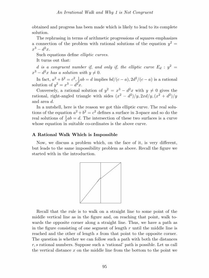
An Irrational Walk and Why 1 is Not Congruent
obtained and progress has been made which is likely to lead to its completesolution.
The rephrasing in terms of arithmetic progressions of squares emphasizesa connection of the problem with rational solutions of the equation y2 =x3 − d2x.
Such equations define elliptic curves.It turns out that:
d is a congruent number if, and only if, the elliptic curve Ed : y2 =x3 − d2x has a solution with y 6= 0.
In fact, a2 + b2 = c2, 12ab = d implies bd/(c− a), 2d2/(c− a) is a rational
solution of y2 = x3 − d2x.Conversely, a rational solution of y2 = x3 − d2x with y 6= 0 gives the
rational, right-angled triangle with sides (x2 − d2)/y, 2xd/y, (x2 + d2)/yand area d.
In a nutshell, here is the reason we got this elliptic curve. The real solu-tions of the equation a2 + b2 = c2 defines a surface in 3-space and so do thereal solutions of 1
2ab = d. The intersection of these two surfaces is a curvewhose equation in suitable co-ordinates is the above curve.
A Rational Walk Which is Impossible
Now, we discuss a problem which, on the face of it, is very different,but leads to the same impossibility problem as above. Recall the figure westarted with in the introduction.
###
##
Recall that the rule is to walk on a straight line to some point of themiddle vertical line as in the figure and, on reaching that point, walk to-wards the opposite corner along a straight line. Thus, we have a path asin the figure consisting of one segment of length r until the middle line isreached and the other of length s from that point to the opposite corner.The question is whether we can follow such a path with both the distancesr, s rational numbers. Suppose such a ‘rational’ path is possible. Let us callthe vertical distance x on the middle line from the bottom to the point we
95

An Irrational Walk and Why 1 is Not Congruent
reach on it. Of course, the rest of the vertical distance is 1− x. Now,
r2 − 1
4= x2
s2 − 1
4= (1− x)2
This gives 2x = 1+r2−s2, which is then rational. Then, writing r = p/qand s = u/v, we have two equations√
4p2 − q2
2q= x
√4u2 − v2
2v= 1− x
Therefore, since the above square-roots are rational, they must be in-tegers and so, q = 2Q (if q were odd, the number 4p2 − q2 would be −1modulo 4 which cannot be a square).
Thus,
x =
√p2 −Q2
2Q=
l
2Q
for some l with (l, Q) = 1.Similarly, v = 2V and
1− x =
√u2 − V 2
2V=
m
2V
with (m,V ) = 1.Thus,
1 =l
2Q+
m
2V
gives 2QV = lV + mQ.As (l, Q) = 1 = (m,V ), we get Q|V, V |Q; that is, Q = V as both are
positive integers.Hence, we have obtained l2 + Q2 = p2,m2 + Q2 = u2, l + m = 2Q with
(l, Q) = 1 = (m,Q).We show that this set of equations does not have any integral solutions.
We could try to use a characterization of primitive Pythagorean triples andproceed but we take another approach. Now, the trivial identity (l+m)2 +(l −m)2 = 2(l2 + m2) gives, on multiplication by (l + m)2 that
(l + m)4 + (l2 −m2)2 = 2(l + m)2(l2 + m2).
96

An Irrational Walk and Why 1 is Not Congruent
The reason to do this is that we have an expression in terms of p, uand Q as follows. Indeed, putting l + m = 2Q, l2 − m2 = p2 − u2 andl2 + m2 = p2 + u2 − 2Q2, we have
16Q4 + (p2 − u2)2 = 8Q2(p2 + u2 − 2Q2).
In other words,
4Q4 − (p2 + u2)Q2 +(p2 − u2)2
8= 0.
This means that the discriminant (p2+u2)2−2(p2−u2)2 = 6p2u2−p4−u4
must be a perfect square, say d2. But then the general algebraic identity
(p2 + u2)4 − (6p2u2 − p4 − u4)2 = (4pu(p2 − u2))2
tells us that (p2 + u2, d, 4pu(p2− u2)) is an integer solution of the equationX4 − Y 4 = Z2. As we already saw, this has only the trivial solution whenY is 0. Note that d = (p2 + u2)2 − 2(p2 − u2) 6= 0 since
√2 is irrational.
Therefore, we have shown that a rational walk as above is impossible forthe same reason that 1 is not a congruent number; viz., that the Fermatequation X4 − Y 4 = Z2 does not have integral solutions with Y 6= 0. Itwould be interesting to directly relate the above ‘rational walk’ problem tothe congruent number problem for 1!
97


Covering the Integers
Let f : N→ C be an arithmetic function. Then, f can be recovered backfrom the function (its Mobius transform) f(n) =
∑d|n f(d) by the Mobius
inversion formulaf(n) =
∑d|n
µ(d)f(n/d),
where the Mobius function is defined µ(n) = 1 if n = 1, µ(n) = (−1)r ifn = p1p2 · · · pr for distinct primes p1, · · · , pr and µ(n) = 0 if not. Here is anelementary observation (in the spirit of the uncertainty principle as madeby Paul Pollack):
Lemma. Let f be any non-zero arithmetic function such that the support
n : f(n) 6= 0,
is a finite set. Then, the support
n : f(n) 6= 0,
of f is infinite.
Proof. Suppose f is non-zero and that n : f(n) 6= 0 is finite. Then,F (z) :=
∑n≥1 f(n)zn is a non-zero polynomial. But, if M = Max(|f(n)| :
n ≥ 1), then for |z| < 1, we have
|F (z)| = |∑n
(∑d|n
f(d))zn| ≤∑n
∑d|n
|f(d)||z|n
≤∑n
(∑d|n
M)|z|n ≤M∑n
n|z|n =m|z|
1− |z|2<∞.
Therefore, we can interchange the summations to obtain
F (z) =∑r
∑d|n
f(d)zrd =∑r
∑d|n
f(d)zd
1− zd.
Now, if N = Max(n : f(n) 6= 0), then F (z) clearly has a pole at z =e2iπ/N which contradicts the fact that F is an entire function.
This gives a proof of the infinitude of primes as follows.
The chapter is a modified version of an article that first appeared in Resonance, Vol. 17, No. 3,pp. 284–290, March 2012.
99

Covering the Integers
Note that µ(n) =∑
d|n µ(d) = 0 for n > 1. So, µ has finite support.So, if there were only finitely many primes, µ would have finite supportcontradicting the ‘uncertainty’ result proved above.
The above type of argument has interesting applications to what areknown as covering congruences. These can be described as follows.
Just as every natural number is either odd or even, one can see that forany k, the congruencesx ≡ 1 (mod 2), x ≡ 1 (mod 4), · · · , x ≡ 1 (mod 2k), x ≡ 0 (mod 2k)
cover the set of all integers. In other words, every integer satisfies at leastone of these congruences. Similarly, for any positive integer N , the set ofcongruences x ≡ i (mod N) for i = 0, 1, · · · , N − 1 covers the integers.
Thus, these are called sets of ‘covering congruences’. The general defini-tion is the following.
Let a1, · · · , ak be integers and let n1, · · · , nk be positive integers. Theset of congruences x ≡ ai (mod ni) for i = 1, · · · , k is called a set ofcovering congruences if Z =
⋃ki=1(ai + niZ). We write the set in short as
a1(n1), a2(n2), · · · ,ak(nk).
Note that in both the cases above, the ‘moduli’ n1, · · · , nk of the congru-ences have the property that
∑ki=1
1ni
= 1.A set of covering congruences a1(n1), · · · , ak(nk) is called a disjoint cov-
ering system if every integer satisfies exactly one of the congruences x ≡ ai(mod ni).
Note that the two sets of covering congruences above, viz.,
1(2), 1(22), · · · , 1(2k), 0(2k)
and0(N), 1(N), · · · , N − 1(N)
are disjoint covering systems. Note also that at least two of the moduli arethe same. That this must always be true is the assertion of the followingproposition whose proof follows the method we started the article with.
PROPOSITION
Let a1(n1), a2(n2), · · · , ak(nk) be a disjoint system of covering congru-ences where n1 ≤ n2 ≤ · · · ≤ nk. Then, nk−1 = nk. Moreover
∑kj=1
1nj
= 1.
Proof. We may assume without loss of generality that 0 ≤ aj < nj foreach j ≤ k. By the hypothesis, we have for |z| < 1,
k∑j=1
zaj
1− znj=
k∑j=1
∞∑r=0
zaj+rnj =∑n≥0
zn =1
1− z.
100

Covering the Integers
Thus, this function has a pole at the point z = 0. But, if ni < nk for alli < k, then this function has a pole at z = e2iπ/nk , a contradiction. Thisproves the first assertion.
Let n = LCM(n1, · · · , nk). Then, we have
1− zn =
k∏j=1
(1− e2iπaj/njzn/nj ),
as each n-th root of unity is a simple root of the polynomial on the lefthand side. This can be rewritten as
1− zn =∑
I⊂1,··· ,k
(−1)|I|z∑
j∈S n/nje2iπ∑
j∈I aj/nj .
Comparing degrees gives us∑k
j=1nnj
= n which is the second assertion.
This leaves the question of the existence of a covering system (necessarilynot disjoint by the above proposition) with distinct moduli. The first setof covering congruences for which the moduli are distinct was given by ASchinzel. This is the set
0(2), 0(3), 1(4), 5(6), 7(12).
Here are two famous conjectures due to Erdos and others which are stillopen.
Conjecture 1. (Erdos-Selfridge). There is no finite system of coveringcongruences where all the moduli are distinct and odd.
Conjecture 2. (Erdos) For any M > 0, there exists a system of coveringcongruences where all the moduli are distinct and > M .
Erdos mentioned in 1995 that the last conjecture is perhaps his favouriteproblem!
We finish with a number-theoretic application which originally motivatedthe study of covering congruences. This is the following beautiful result dueto (who else but!) Erdos.
Theorem. (Erdos, 1950). There are infinitely many odd integers whichare not expressible as the sum of a prime and a power of 2.
Proof. Consider a covering system of congruences ai(ni) with 1 ≤ i ≤ kwhere p1, · · · , pk are distinct odd primes and ni the least positive numbersatisfying 2ni ≡ 1 mod pi.
Erdos constructed such covering systems explicitly; one such is
0(2), 0(3), 1(4), 3(8), 7(12), 23(24)
101

Covering the Integers
Note that the ni’s here – 2, 3, 4, 8, 12, 24 – are the orders of 2 modulo theprimes 3, 7, 5, 17, 13, 241.
Given any such system, the Chinese remainder theorem provides a com-mon solution to the congruencesx ≡ 2ai (mod pi); 1 ≤ i ≤ k and x ≡ 1 (mod 2).Such a solution x is unique modulo 2
∏ki=1 pi. Consider the smallest pos-
itive integer solution, say x0. Now, for each integer r, there exists some isuch that r ≡ ai (mod mi).
So, if n ≡ n0 (mod 2p1 · · · pk), thenn− 2r ≡ n0 − 2ai ≡ 0 (mod pi).Thus, if n− 2r > pi, then it must be composite.This proves that all n not of the form 2r + pi for some r and some i ≤ k
are inexpressible in the form asserted. To dispose of the exceptional cases,we may impose extra congruence conditions.
An example (taking the above covering system 0(2), 0(3), 1(4), 3(8), 7(12),23(24) of Erdos) gives us:
No integer ≡ 7629217 (mod 1184810) is a sum of a power of 2 and anodd prime.
Z-W Sun has done substantial work in the subject of covering congru-ences and revealed connections with zero-sum problems. We finish witha following amazing application completed by Sun of the above work byErdos and later work of Cohen, Selfridge on covering congruences.
Consider the 29-digit number
M = 66483084961588510124010691590
= 2.3.5.7.11.13.17.19.31.37.41.61.73.97.109.151.241.257.331.
Then, the solutions of the congruence
x ≡ 47867742232066880047611079 mod M
cannot be expressed as ±pa ± qb where p, q are primes and a, b are non-negative integers.
As can be readily imagined, simple questions for integers arising out ofcovering systems of congruences have many interesting analogues for groupswhere the congruences are replaced by cosets of subgroups. That will be atopic to discuss on another occasion.
102
S Chowla and S S Pillai:The Story of Two PeerlessIndian Mathematicians1
Ramanujan may be a household namein our country, but it is a shamethat not much is known about who later came.Here, we talk about Chowla and Pillaiwhose names in the mathematical landscape will lieright at the top Any doubts? Illai Illai!
Sarvadaman Chowla (1907–1995) and S S Pillai (1901–1950) were twoof the foremost mathematicians to emerge from India in the generationimmediately after Ramanujan. The Mathematics Geneology Project listsboth Ramanujan and Chowla among the students of Littlewood! This arti-cle specially features Chowla and Pillai. As a matter of fact, the June 2004issue of Resonance journal had already featured Pillai [1] but we shall seethat a discussion of Chowla is necessarily intertwined with one of Pillai.It has been mentioned by G H Hardy that after Ramanujan, the great-est Indian mathematician was Pillai. We journey through some of the veryinteresting and illuminating correspondences between Chowla and S S Pillaiwhich reveals also other personal and historical aspects. Apart from that,we talk about Chowla’s and Pillai’s mathematical works. In a book of thistype, it is essential to select only those topics which are more elementaryor easy to describe while conveying some of the beauty and depth of theideas. Fortunately, in the works of Chowla and Pillai, we can find a verita-ble treasury which is accessible at a level which can be enjoyed by even thenon-expert. Each of their works has an element of surprise and an elementof elegance and simplicity. They worked on a wide spectrum of areas ofnumber theory. We select some of their more elementary gems and discusstheir proofs. In fact, we attempt to retain as much of the original ideas inthe arguments as possible.
It is an enigma that even a layman may ask a question in elementary num-ber theory which turns out to be nontrivial. The fact that several old prob-lems in elementary number theory remain unsolved to this day, has beenreferred to in different ways by people. To quote Professor K Ramachandra,
The chapter is a modified version of an article that first appeared in Resonance, Vol. 17, No. 9,
pp. 855–883, September 2012.1This chapter was part of an article written in collaboration with R Thangadurai.
103

The Story of Two Peerless Indian Mathematicians
“in figurative terms, what has been solved can be likened to an egg-shell, andwhat remains to be solved to the infinite space surrounding it.”
2. Chowla to Pillai Correspondence
Starting in the late 1920s, and up to one month before Pillai’s death,Chowla and Pillai maintained regular correspondence. They published jointpapers starting in 1930 with a famous piece of work on the Euler’s totientfunction. Some other themes that they collaborated on were concerned withsolutions to the Brahmagupta–Pell equation and the Waring problem. Thecorrespondence between these two stalwarts is mathematically illuminatingto read. It also reveals the intellectual honesty they possessed and the joyeach drew from the other’s successes.
104

The Story of Two Peerless Indian Mathematicians
105

The Story of Two Peerless Indian Mathematicians
106

The Story of Two Peerless Indian Mathematicians
The letter shows the reluctance on Chowla’s part to be a co-author ofsome result where he felt he had not contributed enough. The letter iswritten by Chowla after he joined St.Stephen’s College in Delhi. Throughthe years, Chowla consistently expresses almost in every letter his gladnessfor the correspondence between them!
The number theorist K Ramachandra spoke of his first meeting withChowla at the Institute for Advanced Study in Princeton during the
107

The Story of Two Peerless Indian Mathematicians
former’s first visit there. After discussing mathematics, Chowla got themboth bottles of ‘pepsi’ from a vending machine. After the meeting,Ramachandra says that he ran around the premises muttering that he drankpepsi with Chowla!
Chowla’s fertile imagination earned him the sobriquet of ‘poet of mathe-matics’ from his associates. Chowla passed away in the U.S. in 1995 at theage of 88. On the other hand, Pillai died tragically at the age of 49 in 1950.Pillai was invited to visit the Institute for Advanced Study in Princetonfor a year. The flight which he boarded to participate in the 1950 Inter-national Congress of Mathematicians tragically crashed near Cairo on the31st of August. The readers are directed to Pillai’s collected works whichhave appeared recently.
3. Mathematical Gems from Chowla and Pillai
Waring’s Problem
A discussion of Pillai’s mathematical work must start with Waring’sproblem and vice versa! However, since this has been written about indetail in the June 2004 issue, we mention this problem in passing and referthe readers to the above-mentioned Resonance article by C S Yogananda[2].
Waring’s problem asks for the smallest number g(k) corresponding toany k ≥ 2 such that every positive integer is a sum of g(k) numbers eachof which is the k-th power of a whole number. Hilbert had shown that sucha finite number g(k) does exist. The ideal Waring’s conjecture predictsa particular value of g(k). Indeed, if 3k is divided by 2k, the quotient is[(3/2)k], and some remainder r, where [t] denotes the greatest integer lessthan or equal to t. Now, the number
2k[(3./2)k]− 1 = ([(3/2)k]− 1)2k + (2k − 1)1k
is a sum of 2k + [(3/2)k]− 2 numbers which are k-th powers and is not thesum of a smaller number of k-th powers. Hence,
g(k) ≥ 2k + [(3/2)k]− 2.
This ideal Waring conjecture asserts that this lower bound is the cor-rect bound also. Pillai proved, among other things, that this ideal Waringconjecture holds good under the condition on k that the remainder r ondividing 3k by 2k satisfies r ≤ 2k − [(3/2)k] − 2 (chapter 21 of [3]). Thisis known to hold for all k ≤ 471600000. At this time, the ideal Waringconjecture is known to hold for all large enough k.
108

The Story of Two Peerless Indian Mathematicians
4. The Least Prime Quadratic Residue
Chowla’s lifelong pre-occupation with class number of binary quadraticforms led him to discover some rare gems on the way, so to speak! An inter-esting problem, useful in cryptography, for instance, is to find for a givenprime p, the smallest prime q which is a quadratic residue (that is, a square)modulo p. For example, the quadratic reciprocity law tells us that if p ≡ ±1modulo 8, then 2 is the least quadratic residue mod p. Chowla [4] provedthe following beautiful result:
Let p > 3 be a prime such that p ≡ 3 mod 8. Let l(p) denote the leastprime which is a quadratic residue mod p. If the number h(−p) of classes
of binary quadratic forms of discriminant −p is at least 2, then l(p) <√
p3 .
If h(−p) = 1, then l(p) = p+14 (and, therefore, p+1
4 is prime!).
Remarks. (i) The theorem implies, in particular, that for primes p > 3,
p ≡ 3 mod 8, we have l(p) = p+14 if and only if h(−p) = 1 because
√p3 <
p+14
for p > 3.(ii) The proof of the theorem is easy and uses Minkowski’s reduction
theory of quadratic forms which produces in each equivalence class ofpositive-definite forms, a unique one ax2 + bxy + cy2 which is ‘reduced’in the sense that |b| ≤ a ≤ c.
5. Chowla’s Counter-examples to a Claim of Ramanujan and aDisproof of Chowla’s Conjecture
Among Ramanujan’s numerous astonishing results, there are also occa-sional lapses. One such was his ‘proof’ (in his very first paper of 1911) thatthe numerators of Bernoulli numbers are primes. This is false; for instance,denoting by Bn the Bernoulli number defined by
z
ez − 1=∑n≥0
Bnzn
n!,
and by Nn, the numerator of Bn/n, the numbers N20, N37 are composite.In 1930, Chowla showed [5] that Ramanujan’s claim has infinitely manycounter-examples. Surprisingly, Chowla returns to this problem 56 yearslater(!) in a joint paper with his daughter [6] and poses as an unsolvedproblem that Nn is always square-free. In a recent article, Dinesh Thakur[7] points out that Chowla’s question has infinitely many negativeanswers. Indeed, Thakur shows:
For any fixed irregular prime p less than 163 million, and any arbi-trarily large k, there exists a positive integer n such that Nn is divisibleby pk.
109
The Story of Two Peerless Indian Mathematicians
If we observe (from the existing tables) that 372 divides N284, Chowla’squestion has a negative answer. The proof of the more general assertion usesthe so-called Kummer congruences which essentially assert that the value of(pn−1−1)Bn
n modulo pk depends (for even n) only on n modulo pk−1(p− 1),if p − 1 does not divide n. Using this as well as certain functions calledp-adic L-functions, the general assertion of arbitrarily large powers canalso be obtained.
6. Problem on Consecutive Numbers
Pillai proved in 1940 that any set of n consecutive positive integers wheren ≤ 16, contains an integer which is relatively prime to all the others.However, there are infinitely many sets of 17 consecutive integers wherethe above fact fails. For instance, N +2184, N +2185, · · · , N +2200 is sucha set whenever N is a multiple of 2.3.5.7.11.13 = 30, 030. Moreover, Pillaialso proved [8] that for any m ≥ 17, there are infinitely many blocks of mconsecutive integers for which the above property fails. Now, generalizationsto arithmetic progressions instead of consecutive numbers are known.
7. How Spread-out are Perfect Powers?
Look at the sequence of all perfect powers of positive integers:
1, 4, 8, 9, 16, 25, 27, 32, 36, 49, 64, 81, 100, 121, 125, · · · .
We observe that differences between consecutive terms can be: 1 (9− 8),2 = (27− 25), 3 (4− 1), 4 (36− 32), 5 (32− 27) etc.
Pillai conjectured that consecutive terms can be arbitrarily far apart [9].In other words, given any number, one can find consecutive terms whosedifference is larger than that given number. Equivalently, the conjectureasserts:
Given a positive integer k, the equation xp − yq = k has only finitelymany solutions in positive integers x, y, p, q ≥ 2.
This is unproved as yet even for one value of k > 1 although it is knownnow that if one of these 4 parameters is fixed, the finiteness holds.
8. Independent Values of the Cotangent Function
A typical aspect of Chowla’s works has been to come back to an old resultafter several years and applying it in an unexpected manner. On 9.2.1949,Chowla had written to Carl Ludwig Siegel about a certain non-vanishing ofa particular type of series. Three days later, he received a reply from Siegel,improving the result. In 1970, Chowla, while wondering about relationsbetween the roots of a certain polynomial, realized that not only could he
110

The Story of Two Peerless Indian Mathematicians
re-prove Siegel’s improved version in a simpler fashion [10], he could usethis old result to prove what he wanted about the roots! Let us discuss itbriefly.
If p is a prime number, consider the values xr = cot(rπ/p) of the cotan-gent function, for 0 < r < p. Evidently, xr + xp−r = 0. Also,
∑p−1r=1 xr = 0
but this is easily deduced from the earlier relations. So, a natural ques-tion is:
Are all the linear relations of the form∑p−1
i=1 arxr = 0 with ai ∈ Q,consequences of the relations xr + xp−r = 0 for 1 ≤ r < p?
Indeed, xr’s are the roots of an irreducible polynomial over Q, of degreep− 1 and, one may ask for possible linear relations among the roots of anyirreducible polynomial over Q. Chowla’s theorem asserts:
Let p be a prime number and xr = cot(πr/p) for r = 1, · · · , p−12 . If ai ∈ Q
such that∑ p−1
2i=1 aixi = 0, then ai = 0 for all i ≤ (p− 1)/2.
Chowla uses some very basic Galois theory to deduce that, under the as-
sumption∑ p−1
2i=1 aixi = 0 above, there are (p−1)/2 such linear relations, viz.,
a1x1 + a2x2 + · · ·+ a p−32x p−3
2+ a p−1
2x p−1
2= 0
a1x2 + a2x3 + · · ·+ a p−32x p−1
2+ a p−1
2x1 = 0
...
a1x p−12
+ a2x1 + · · ·+ a p−12x p−3
2= 0.
If the ai’s are not all 0, this leads to the vanishing of the ‘cirulant’determinant
x1 x2 · · · x(p−1)/2
x2 x3 · · · x1
. . .. . .
x(p−1)/2 x1 · · · x(p−3)/2
.
At this point, Chowla quotes the well-known value of this determinantand proceeds.
What is the value of this determinant?In the 3× 3 case x1 x2 x3
x2 x3 x1
x3 x1 x2
,
has determinant 3x1x2x3 − x31 − x3
2 − x33.
Let 1, ω, ω2 be the cube roots of unity.If x1, x2, x3 are replaced by ωx1, ω
2x2, x3 or by ω2x1, ωx2, x3, the expres-sion remains the same. As x3 = −x1−x2 leads to 3x1x2x3−x3
1−x32−x3
3 = 0,
111

The Story of Two Peerless Indian Mathematicians
the three expressions x1 + x2 + x3, ωx1 + ω2x2 + x3, ω2x1 + ωx2 + x3 are
factors. In other words, the determinant in the 3× 3 case is given as:
det
x1 x2 x3
x2 x3 x1
x3 x1 x2
= −(x1 +x2 +x3)(ωx1 +ω2x2 +x3)(ω2x1 +ωx2 +x3).
Similarly, in general, the determinant of
x1 x2 · · · x(p−1)/2
x2 x3 · · · x1
. . .. . .
x(p−1)/2 x1 · · · x(p−3)/2
equals the product (up to sign) of
ωrx1 + ω2rx2 + · · ·+ ωr(p−1)
2 x p−12
as r varies from 1 to p−12 where ω = e
4iπp−1 , (p− 1)/2-th root of unity.
Here, Chowla realizes with surprise that the above factors are (up tocertain non-zero factors) none else other than the special value at s = 1
of certain functions L(s, χ) =∑∞
n=1χ(n)n called Dirichlet L-functions cor-
responding to Dirichlet characters χ modulo p which satisfy χ(−1) = −1.The non-vanishing of these are the older result mentioned above and show,thus, that the determinant is non-zero. Hence, the linear independence ofthe cot(rπ/p) for 1 ≤ r ≤ (p− 1)/2 is established.
Remarks. (i) Kai Wang closely followed Chowla’s proof to generalize histheorem to non-primes and to derivatives of the cotangent function [11] byshowing:
For any s ≥ 0 and an arbitrary natural number k, the φ(k)2 real numbers
ds
dxs cot
(x+ rπ
k
)x=0
(where r ≤ φ(k)2 and (r, k) = 1) are linearly independent
over Q.
(ii) The non-vanishing at s = 1 of L(s, χ) for nontrivial Dirichlet char-acters is the key fact used in the proof of Dirichlet’s famous theorem onexistence of infinitely many primes in any arithmetic progression an + bwith (a, b) = 1.
(iii) Kenkichi Iwasawa (see [12]) showed later in 1975 that the aboveresult has connections with the so-called “regular” primes. The definitionof regular primes is not needed here and, we merely recall that Kummer hadproved that the Fermat equation xp + yp = zp has no non-zero solutionsin integers if p is a ‘regular prime’. It is unknown yet whether there areinfinitely many regular primes (although Fermat’s last theorem has beenproved completely) – surprisingly, it has been known for a long time thatthere are infinitely many irregular primes! The connection of the aboveresult of Chowla with regular primes is the following.
112

The Story of Two Peerless Indian Mathematicians
The linear independence of the (p − 1)/2 cotangent values ensures thatthere exist rational numbers t1, · · · , t p−1
2so that
2 sin2π
p=
p−12∑
r=1
tr cot(2rπ/p).
Iwasawa shows the prime p is regular if and only if, none of the tr’s havedenominators which is a multiple of p and, at least one tr has numeratoralso not divisible by p.
9. On the Number of Permutations of a Given Order
Chowla wrote a series of papers on generating functions for the number ofpermutations of a given order etc. In the permutation group Sn, let An(d)denote the number of permutations σ satisfying σd = Id. In collaborationwith Herstein and Scott, he showed ([13]):
∞∑n=0
An(d)xn
n!= exp(
∑k|d
xk
k).
Here, convenience of notation, one takes A0(n) = 1. Let us prove thisbeautiful, useful fact.
We look for a recursive relation for An(d) in terms of Ak(d) for k < n.Look at what happens to the symbol n under any permutation contribut-ing to An(d). If the symbol is fixed, then the rest of the n− 1 symbols canbe permuted in An−1(d) ways. Now, suppose the symbol n is a part of ak-cycle for some 1 < k ≤ n. Note that any permutation contributing toAn(d) has some order dividing d; thus, if it has a k-cycle in its decompo-sition, then k|d. Now, each k-cycle contributes An−k(d) elements. As thereare (n− 1)(n− 2) · · · (n− k + 1) ways to choose such k-cycles, we get
An(d) = An−1(d) +∑
k|d;1<k≤n
(n− 1) · · · (n− k + 1)An−k(d).
This can be rewritten as
An(d)
n!=
∑k|d;1≤k≤n
An−k(d)
(n− k)!.
Therefore, the generating function f(x) =∑
n≥0An(d)n! satisfies
xf ′(x) =∑i≥1
Ai(d)xi
i!=∑i≥1
( ∑k|d,1≤k≤i
Ai−k(d)
(i− k)!
)xi,
on using the recursion above.
113

The Story of Two Peerless Indian Mathematicians
Combining the terms corresponding to a particular Aj(d), we havetherefore
xf ′(x) =∑j≥0
Aj(d)
j!
∑k|d
xj+k = f(x)∑k|d
xk.
This is a differential equation
f ′(x)
f(x)=∑k|d
xk−1
whose general solution is obtained by integration as
f(x) = c.exp
(∑k|d
xk
k
)
for some constant c. Since f(0) = A0(d) = 1 = c, we get the assertion
∑n≥0
An(d)
n!= exp
∑k|d
xk
k
.
This formula is useful in a number of ways. For instance, one can getan asymptotic estimate of how fast An(d) grows with n (for any fixed d).Moreover, for d = p, a prime, this gives a simple-looking closed formula forAn(p) for any n.
9.1 Closed Form for the Prime Case
In the above identity
∑n≥0
An(d)
n!= exp
∑k|d
xk
k
.
take d = p, a prime and note that∑n≥0
An(p)
n!= exex
p/p =∑i≥0
xi
i!
∑j≥0
xpj
pjj!.
Comparing the coefficients of xn, we obtain
An(p) =∑
i+pj=n
n!
pjj!i!.
In particular, this number is a positive integer for each n ≥ p(!)This is an exclamation mark, not a factorial!
114

The Story of Two Peerless Indian Mathematicians
Also, a classical theorem in the theory of groups, due to Frobenius, assertsthat in any finite group G, the number of elements satisfying xd =identity(for any divisor d of the order of G) is a multiple of d. Thus, we have An(d)is a multiple of d for each n ≥ d.
This statement for An(p) gives, therefore, that∑
i+pj=nn!
pjj!i!is a multiple
of p for every n ≥ p and, the special case n = p is known as Wilson’stheorem.
9.2 Applications to Finite Groups
Apart from being useful in its own right, the study of the numbers An(d)has connections to some counting problems in groups. Notice that the num-ber An(d) of permutations in Sn which satisfy xd = identity, is nothingelse than the number of group homomorphisms from a cyclic group oforder d to Sn – each homomorphism associates a permutation σ satisfyingσd = Identity, to a fixed ‘generator’ of the cyclic group. For any group G(not necessarily cyclic), knowledge of the numbers hn of group homomor-phisms from G to Sn for various n, allows us to find a recursive expressionfor the number of subgroups of G which have a given index in it. In fact,if sn is the number of subgroups of index n in G, then
sn +h1
1!sn−1 +
h2
2!sn−2 + · · ·+ hn−1
(n− 1)!s1 =
hn(n− 1)!
.
10. Convenient Numbers and Class Number
Euler observed that 18518809 = 1972 + 1848(100)2 is a prime. In fact,Euler was interested in producing large primes of the form x2 + ny2 forvarious values of n. It happens (and is easy to prove) that a number whichhas a unique expression of the form x2 + y2 is prime. Thus, one may hopethis is true for expressions of the form x2 + ny2 also for any n. However,as Euler noted [14], this holds only for a certain set of values of n. He con-structed explicitly a set of 65 positive integers for which this is true (thelargest of which is 1848) – he called such numbers ‘idonean’ or ‘convenient’.To this day, it is not proven that Euler’s list is complete [15]. However, abeautiful result of Chowla shows at least that the list of idonean num-bers is finite! To explain how it is done, we very briefly define and dis-cuss binary quadratic forms – another name for expressions of the formax2 + bxy + cy2.
A binary, integral quadratic form is a polynomial f(x, y) = ax2+bxy+cy2
where a, b, c are integers. It is primitive if (a, b, c) = 1. The integer b2− 4acis known as the discriminant.
As
4af(x, y) = (2ax+ by)2 + (4ac− b2)y2 = (2ax+ by)2 − dy2,
115

The Story of Two Peerless Indian Mathematicians
when d < 0 and a > 0, f(x, y) takes only positive values (excepting thevalue 0 at x = y = 0). Thus, when a > 0, and the discriminant is negative,the form is positive-definite.
For example, x2 +ny2 is a positive-definite form with discriminant −4n.Two forms f(x, y) and g(x, y) are said to be equivalent or, said to be in the
same class if f(αx+βy, γx+δy)) = g(x, y) where A =
(α βγ δ
)∈ SL(2,Z),
an integer matrix of determinant 1.The motivation behind this definition is:
Equivalent forms take the same sets of values as x, y vary over integers.
This is clear because one may also write
g(x, y) = f(αx+ βy, γx+ δy))
in the formf(x, y) = g(δx− βy,−γx+ αy)).
Notice that the matrix
(δ −β−γ α
)is simply the inverse of the matrix(
α βγ δ
).
Moreover, equivalent forms have the same discriminant. Gauss showed:
For d < 0, the number h(d) of classes of primitive, positive-definite binaryquadratic forms of discriminant d is finite.
Gauss conjectured that h(d) → ∞ as −d → ∞. This was proved byHeilbronn. By a modification of Heilbronn’s argument, Chowla proved thefollowing fact which was another conjecture of Gauss [16]:
h(d)2t →∞ as −d→∞ where t is the number of primes dividing d.
This interesting fact is useful in a totally different context which weindicate briefly now.
Euler obtained the following list of 65 numbers called ‘Numerus idoneus’(or ‘convenient’ numbers):
1, 2, 3, 4, 5, 6, 7, 8, 9, 10, 12, 13, 15, 16, 18, 21,22, 24, 25, 28, 30, 33, 37, 40, 42, 45, 48, 57, 58,60, 70, 72, 78, 85, 88, 93, 102, 105, 112, 120, 130,133, 165, 168, 177, 190, 210, 232, 240, 253, 273, 280,312, 330, 345, 357, 385, 408, 462, 520, 760, 840, 1320, 1365, 1848.
Consider any odd number m co-prime to n which is expressible asm = x2 + ny2 with (x, ny) = 1. If each such m which has a unique ex-pression of the form x2 + ny2 in positive integers x, y is necessarily prime,the number n is said to be idonean.
116

The Story of Two Peerless Indian Mathematicians
As mentioned in the beginning of this section, Euler observed that18518809 = 1972 + 1848(100)2 is a prime by showing 1848 is idonean.
Firstly, it is not even clear whether the list of idonean numbers is finiteor not. This can be analyzed (and was analyzed by Gauss) using the theoryof quadratic forms.
Firstly, we recall one more notion – the genus.Two primitive, positive-definite forms of discriminant d are said to be
in the same genus if they take the same set of values modulo d. As formsin the same class take the same set of values, they are in the same genus.Each genus, therefore, consists of finitely many classes.
Gauss proved (modulo some gaps which were filled later by Grube):
A positive integer n is idonean if and only if, for forms of discriminant−4n, every genus consists of a single class.
Chowla’s theorem h(d)2t →∞ as −d→∞ where t is the number of primes
dividing d, which was quoted above, implies that for large enough −d, eachgenus has more than one class of forms. Therefore, by Chowla’s theorem,the set of idonean numbers is finite!
As a matter of fact, Euler’s list is expected to be a complete one (thishas been proved to be so under the assumption of a deep conjecture knownas the generalized Riemann hypothesis).
11. Matrices and Quadratic Polynomials
As we saw earlier, the equivalence classes of integral, binary quadraticforms are related to the group SL2(Z) of integral matrices of determinant1. Recall also that equivalent forms take the same sets of integer values asx, y vary over integers. The following result of Chowla with J Cowles andM Cowles [17] shows that the relation is an intimate one. We recall thattwo matrices A,B are said to be conjugate if there is an invertible matrixP such that B = PAP−1. The trace of a matrix is the sum of its diagonalentries. Then:
For all integers t 6= ±2, the number of conjugacy classes of matrices inSL2(Z) with trace t, equals the number of equivalence classes of integral,binary quadratic forms with discriminant t2 − 4.
Recall the discriminant of a quadratic form ax2 + bxy + cy2 was definedin the last section to be the number b2 − 4ac. Here is the easy proof of theabove theorem.
Associate to each matrix M :=
(a bc d
)∈ SL2(Z), the quadratic form
m(x, y) := bx2 + (d− a)xy − cy2.
117

The Story of Two Peerless Indian Mathematicians
Note that if the trace of M is t, then a + b = t and, therefore, thediscriminant of m(x, y) is
(d− a)2 + 4bc = (d+ a)2 − 4(ad− bc) = t2 − 4.
For a conjugate matrix N := AMA−1 where A =
(α βγ δ
)∈ SL2(Z),
write N as
(a′ b′
c′ d′
). Then, the form n(x, y) = b′x2 + (d′ − a′)xy − c′y2 is
easily seen to be m(x′, y′) where(x′
y′
)= At
(xy
)=
(αx+ γyβx+ δy
).
In other words, under the above association, conjugate matrices of tracet correspond to equivalent forms of discriminant t2 − 4.
Conversely, associate to a quadratic form f(x, y) = px2 + qxy+ ry2 withdiscriminant t2 − 4 (so, q2 − 4pr = t2 − 4), the matrix
F :=
( t−q2 p
−r t+q2
)∈ SL2(Z).
Note that indeed, det F = t2−q24 + pr = 1 and trace F = t.
Further, look at any equivalent form f ′(x, y) = f(ax+ by, cx+ dy) with
M :=
(a bc d ∈ SL2(Z)
).
Write f ′(x, y) = p′x2 + q′xy + r′y2.Then, we compute and see that
M tF (M t)−1 =
(a cb d
)( t−q2 p
−r t+q2
)(d −c−b a
)=
(t′−q′
2 p′
−r′ t′+q′
2
),
which shows that the corresponding matrices are conjugate in SL2(Z).The above associations are inverse to each other and proves the proposi-
tion.
Remarks. The above association is also useful in deciding if two matri-
ces are conjugate in SL2(Z) or not. For instance, the matrices
(1 33 10,
)(
1 19 10
)which have trace 11 are associated to the quadratic forms
3x2 + 9xy − 3y2 , x2 + 9xy − 9y2,
respectively. However, they are evidently in-equivalent because the first onetakes only multiples of 3 as values whereas the second one takes values like1 at (x, y) = (1, 0).
118

The Story of Two Peerless Indian Mathematicians
12. Average of Euler’s φ-function
Euler’s φ-function, denoted by φ(n) is an arithmetic function defined onnatural numbers that counts the number of natural numbers 1 ≤ m ≤ nwith (m,n) = 1. Euler gave a formula which can be proved using inclusion– exclusion principle as follows.
φ(n) = n∏p|n
(1− 1
p
),
where the product varies over all the distinct prime divisors. This formulashows that the functional value fluctuates a lot.
In analytic number theory, to study such fluctuating arithmetical func-tions, one often looks at their average behaviour. One can prove that theaverage value from 1 to x is 3
π2x but the interesting part is to have an ideaof the error which would be introduced if we take this value. In analyticnumber theory, this methodology of ‘determining the main term and esti-mating the error term’ is fundamental because we cannot deduce anythingconcrete if the error term is of the same order as the main term! One has∑
1≤n≤xφ(n) =
3
π2x2 + E(x),
where E(x) is the remainder or error term in the average.Dirichlet showed that for any given ε > 0, there is a constant C > 0 so
that |E(x)| ≤ Cx1+ε for all x > 0. Later, this was improved to |E(x)| ≤C ′x log x for all x > 0 by Mertens.
Sylvester prepared a table of values for∑n≤x
φ(n) and3
π2x2 for all x =
1, 2, · · · , 1000. However, he failed to notice that E(820) < 0 and madea conjecture that E(x) ≥ 0 for all x. In 1929, Chowla wrote a letter toPillai where he predicted that E(x) > 0 for infinitely many values of x andE(x) < 0 for infinitely many values of x.
In order to prove an error term, say |E(x)| ≤ cg(x), is tight for somenon-negative function g(x), one needs to produce a positive constant c0
and infinitely many x’s such that |E(x)| > c0g(x).Such a result is called an ‘omega’-result in analytic number theory; we
write E(x) = Ω(g(x)).Chowla and Pillai showed that E(x) = Ω(x log log log x).Such a result took many years to generalize. There is a conjecture by
Montgomery that
E(x) = O(x log log x) and E(x) = Ω±(x log log x),
which is still open.
119

The Story of Two Peerless Indian Mathematicians
13. A Variant of Tic-Tac-Toe!
In 1933, Pillai studied a variant of Tic-Tac-Toe game as follows. Let n ≥ 3be an integer and t ≤ n be another integer. Suppose n × n grid with n2
squares is given in the plane. Let P and Q be two players playing. By turnseach mark a square. The rule of playing the game is as follows. SupposeP is the starter and, let Pr and Qr be the squares marked respectively byP and Q during their r-th turns. After P ’s (or Q’s) s-th turns, whoevermarked t squares in a straight line wins the game.
Pillai proves that when t = n and the game is carefully played, then itwill end always in a draw. However, if t < n, then for a given t, there is afunction f(n) depending on n such that if t ≥ f(n), then the game endsin a draw. When t < f(n), he proved that the player who starts will win.Also, he proved that f(n) ≤ n+ 1−
√n/6 and f(n) = n for all n = 3, 4, 5,
and 6. For large values of n, the correct order of f(n) is still unknown!
14. Smooth Numbers
Smooth numbers are numbers which have only ‘small’ prime factors. Forexample, 1,620 has prime factorization 22×34×5; therefore 1620 is 5-smoothbecause none of its prime factors is greater than 5. Smooth numbers havea number of applications to cryptography. For example, the very smoothhash functions are used constructively to get a provably secure design. Theyalso play a role in music theory apparently (Longuet–Higgins, H C, Letterto a musical friend, Music Review (August: 244-248), 1962!)
For other applications, the interested reader may also consult [18] and [19].For any real numbers x, y > 1 with y ≤ x, we define ψ(x, y) to be the
number of positive integers t ≤ x such that if a prime p|t, then p ≤ y. Inother words, ψ(x, y) counts all the y-smooth numbers up to x. Ramanujan(in a letter to Hardy) was the first to study these smooth numbers wheny = 3(!)
He obtained a nice asymptotic formula for ψ(x, 3).In the 7-th conference of Indian Mathematical Society during 3–5, April,
1931 at Trivandrum, Pillai extended the above result of Ramanujan whichimplies an asymptotic formula for ψ(x, y) if y > 1 is a fixed real number.This is technical to state but we mention it here in passing, for the interestedreader:
If p1, p2, · · · , pr ≤ y are all the prime numbers less than y, then
ψ(x, y)− (log x)r
r!∏ri=1 log pi
+ (log x)r−1 log(p1···pr)2(r−1)!
∏ri=1 log pi
)
logr−1 x→ 0
when x→∞.
120
The Story of Two Peerless Indian Mathematicians
Around that time, Dickman obtained an asymptotic result for ψ(yu, y)for any fixed u > 0. The word ‘asymptotic’ here refers to an assertion ofthe form ‘what is the limit of ψ(yu,y)
yu as u→∞’?A more rigorous proof of Dickman’s result, in modern standards, was sup-
plied by Chowla and T Vijayaraghavan in 1947 where they used an unpub-lished result of Pillai which is more general than the above result of Pillai!
It should be mentioned that Ramanujan – see page 337 of S Ramanujan,The lost notebook and other unpublished papers. Narosa Publishing House,(1988) – had the following entry. We write in the standard notations asabove:
ψ(x, xc) ∼ x
(1−
∫ 1
c
du
u
)if 1/2 ≤ c ≤ 1;
ψ(x, xc) ∼ x
(1−
∫ 1
c
du
u+
∫ 1/2
c
dv
v
∫ 1−v
v
du
u
)if 1/3 ≤ c ≤ 1/2;
ψ(x, xc) ∼ x
(1−
∫ 1
c
du
u+
∫ 1/2
c
dv
v
∫ 1−v
v
du
u−∫ 1/3
c
dz
z
∫ (1−z)/2
z
dv
v
∫ 1−v
v
du
u
)if 1/4 ≤ c ≤ 1/3; and so on.
This is nothing else than Dickman’s asymptotic formula for ψ(x, y)!
15. Chowla’s Argument and the Langlands Conjecture
In this last section, we mention how an argument due to Chowla plays arole in the famous Langlands conjectures. The cognoscenti would know thatthe latter conjectures drive much of the contemporary research in numbertheory [20].
This section is mostly taken from a lecture of Professor Ram Murty atKerala School of Mathematics, Calicut – thanks go to Professor Ram Murtyfor allowing inclusion of the contents in this write up.
For each integer n ≥ 1, define d(n) is the number of positive divisors ofn. In his famous paper on ‘highly composite numbers’, Ramanujan gave anupper bound for the function d(n) as follows:
d(N) ≤ 2logN
log logN for all N ≥ 2
and he produced infinitely many integers N for which the above bound isattained.
For any given ε > 0, we can deduce from the above upper bound thatthere is a constant N0 depending on ε so that
d(N) ≤ N ε for all N ≥ N0.
Chowla proved this deduction using another argument involving Dirichletseries.
121

The Story of Two Peerless Indian Mathematicians
Let r ≥ 1 be any integer and let
Lr(s) =∞∑n=1
dr(n)
nswhere s ∈ C with <(s) > 1.
Chowla observed that the series
Lr(s) =∏p
(1 +
2r
ps+
3r
p2s+ · · ·
)(where the product runs over all the prime numbers) converges absolutelyfor Re(s) > 1 for all r ≥ 1. In particular, when s = 2, this series converges.So,
∞∑n=1
d(n)r
n2<∞ for all integers r ≥ 1.
Therefore, the n-th term which isd(n)r
n2tends to zero. In particular, it
is bounded for all large enough n’s. Thus, we get
d(n)r ≤ cn2 for all n ≥M
for some M > 0 and c > 0 constants and this is true for all r ≥ 1.Thus, for all n ≥M , we get d(n) ≤ c1/rn2/r. Also, note that c1/r → 1 as
r →∞.Given ε > 0, we can find r0 such that 2/r < ε for all r ≥ r0 and we get
d(n) ≤ nε.To show how this sort of argument plays a role in the famous
Langlands conjectures, we describe such a conjecture. This can be donethrough the famous Ramanujan delta function. Ramanujan studied thefollowing q-series
∆(z) = q
∞∏n=1
(1− qn)24 where z ∈ C with =(z) > 0; q = e2πiz
which is often called Ramanujan’s delta function because of his funda-mental contribution to it although it was already studied by Jacobi andothers.
The delta function satisfies the following property:
for all
(a bc d
)∈ SL2(Z) (that is, for integers a, b, c, d with ad− bc = 1),
∆
(az + b
cz + d
)= (cz + d)12∆(z).
122

The Story of Two Peerless Indian Mathematicians
Since
(1 10 1
)∈ SL2(Z) and by the above relation, we see that ∆(z+1) =
∆(z) and hence ∆ function is a periodic function.Therefore, it has a Fourier expansion. It can be proved that the Fourier
expansion of ∆(z) is
∆(z) =
∞∑n=1
τ(n)e2iπnz,
where τ(n) is the Fourier coefficients which are integers.Traditionally, one writes q = e2iπz so that ∆(z) =
∑∞n=1 τ(n)qn.
Ramanujan computed the initial τ values and conjectured the followingrelations.
1. τ(mn) = τ(m)τ(n) whenever (m,n) = 1.2. τ(pa+1) = τ(p)τ(pa)− p11τ(pa−1) for all primes p and a ≥ 1.3. |τ(p)| < 2p11/2 for every prime p.
The first two conjectures were proved by Mordell in 1917 and the third onewas proved by P Deligne in 1975 using deep algebraic geometry.
Note that the third conjecture of Ramanujan is equivalent to theassertion:
τ(n) = O(n112
+ε)
for any given ε > 0.Our interest is in this version of Ramanujan’s conjecture.Let us define for each integer n ≥ 1,
τn = τ(n)/n11/2.
Then Ramanujan’s conjecture is equivalent to τn = O(nε) for any givenε > 0. Define the L-series attached to ∆ function as
L(s,∆) =∞∑n=1
τnns,
where s ∈ C with =(s) > 0.Since τ(n) is a multiplicative function (the first conjecture of Ramanujan
mentioned above and proved by Mordell), we see that τ rn is also a multi-plicative function and hence we get
L(s,∆) =∏p
(1 +
τpps
+τp2
p2s+ · · ·
).
Using the second conjecture of Ramanujan, one notes that for all primesp, we have
∞∑a=0
τpaXa =
1
1− τpX +X2=
1
(1− αpX)(1− βpX),
123

The Story of Two Peerless Indian Mathematicians
where αp and βp are the complex roots of X2 − τpX + 1. Note thatαp + βp = τp and αpβp = 1.
L(s,∆) =∏p
(1− αp
ps
)−1(1− βp
ps
)−1
=∏p
1∏m=0
(1−
α1−mp βmpps
)−1
.
For any r ≥ 1, Langlands defined the function:
Lr(s,∆) =∏p
r∏m=0
(1−
αr−mp βmpps
)−1
.
He conjectured that for every r ≥ 1, Lr(s,∆) defines a series which isabsolutely convergent for <(s) > 1.
Note that the Dirichlet series
Sr :=∞∑n=1
τ2rn
ns
can be written as a product of the Lk(s,∆) for k ≤ r. Therefore, if theconjecture of Langlands is true, then Sr converges absolutely for <(s) > 1for every r ≥ 1. This implies, by Chowla’s argument, that
τ2rn
n2≤ C ⇐⇒ τn ≤ C1/2rn1/r
for all n ≥ n0. Thus, we arrive at τn = O(nε) for any given ε > 0 (!).However, at present Langlands’s conjecture is known only for all r ≤ 9.
Collected works of Chowla and of Pillai:
The collected works of Chowla and of Pillai contain unpublished papersalso. The interested readers can look at:
• Collected works of S Chowla, Vol.1,2,3, Edited by James G Huardand Kenneth S Williams, CRM Univ. de Montreal, 1999.
• Collected works of S S Pillai, Edited by R Balasubramanian andR Thangadurai, Ramanujan Mathematical Society Collected WorksSeries, 2010.
References
[1] B Sury, Box 1, Resonance, Vol. 9, No. 6, 2004.[2] Waring’s problem and the circle method, Resonance, Vol. 9, No. 6,
pp.51–55, 2004.
124

The Story of Two Peerless Indian Mathematicians
[3] G H Hardy and E M Wright, An introduction to the theory of numbers,Oxford Univ. Press, third ed., 1954.
[4] S Chowla, The least prime quadratic residue and the class number,J. Number Theory, 22, 1–3, 1986.
[5] S Chowla, On a conjecture of Ramanujan, Tohoku Math. J. 33, 1–2,1930.
[6] S Chowla and P Chowla, Some unsolved problems, Norske Vid. Selsk.Forth. (Trondheim), p.7, 1986.
[7] D Thakur, A note on numerators of Bernoulli numbers, Proc. Amer.Math. Soc., Electronically published on 24.02.2012.
[8] S S Pillai, On a linear diophantine equation, Proc. Indian Acad. Sci.A, 12, pp.199–201, 1940.
[9] S S Pillai, On the inequality 0 < ax − by ≤ n, Journal Indian M. S.,19, pp. 1–11, 1931.
[10] S Chowla, The nonexistence of nontrivial linear relations between theroots of a certain irreducible equation, J. Number Theory, 2, 120–123,1970.
[11] Kai Wang, On a theorem of Chowla, J. Number Theory, 15, 1–4, 1982.[12] Raymond Ayoub, On a theorem of Chowla, J. Number Theory, 7,
108–120, 1975.[13] S Chowla, I N Herstein and W R Scott, The solutions of xd = 1 in
symmetric groups, Norske Vid. Selsk. Forth. (Trondheim) 25, 29–31,1952.
[14] L Euler, De Formulis specei mxx+ nyy ad numeros primos exploran-dos idoneis earumque mirabilis proprietatibus, Opera Omnia I, v. 4,Teubner, pp. 269–289, 1916.
[15] G Frei, Leonhard Euler’s convenient numbers, Math. Intell., 7, No. 3,55–58, 64, 1985.
[16] S Chowla, An extension of Heilbronn’s class-number theorem, Quart.J. Math., 5, 304–307, 1934.
[17] S Chowla, J Cowles and M Cowles, J.Number Theory, 12, 372–377,1980.
[18] A Granville, Smooth numbers: Computational number theory andbeyond, Proceedings of an MSRI workshop, 2004.
[19] A Hildebrand and G Tenenbaum, Integers without large prime factors,J. Theor. Nombres Bordeaux, 5, No. 2, 411–484, 1993.
[20] Ram Murty, Topics in Number Theory, Mehta Research InstituteLecture Note No. 1, 1993.
125


Multi-variable ChineseRemainder Theorem
1. Introduction
The Chinese remainder theorem (CRT) seems to have originated in the3rd century AD in the work of Sun-Tsu. There are also versions in Indian5th century mathematics of Aryabhata. The classical versions dealt withcoprime moduli. Oystein Ore proved a version [1] for non-coprime moduliin 1952 in the American Mathematical Monthly but, this does not seemto be well-known because a paper published 50 years later by Howard [2]proves the same result! However, a multi-variable version does not seemto be known. We present such a version and point out that there are stillmany questions open for investigation.
2. Classical CRT
A variant of a folklore tale goes as follows. Three thieves steal a numberof gold coins and go to sleep after burying the loot. During the night, onethief wakes up and digs up the coins and, after distributing into 6 equalpiles, finds 1 coin left over which he pockets quietly after burying the restof the coins. He goes back to sleep and after a while, a second thief wakesup and digs up the coins. After making 5 equal piles, he again finds 1 coinleft over which he pockets and buries the rest and goes to sleep. The 3rdthief wakes up and finds the rest of the coins make 7 equal piles exceptinga coin which he pockets. If the total number of coins they stole is not morethan 200, what is the exact number?
With a bit of hit and trial, one can find that 157 is a possible number.The Chinese remainder theorem gives a systematic way of solving this ingeneral.
In the above problem, the sought-for natural number N is so that N − 1is a multiple of 6, N −2 is a multiple of 5 and N −3 is a multiple of 7. Thismeans that N leaves remainders 1, 2, 3 on division by 6, 5, 7 respectively.
Let us consider two coprime natural numbers m1,m2 and suppose, we arelooking for a natural number N which leaves remainders a1, a2 on divisionby m1,m2 respectively. Then, the Euclidean division algorithm tells us that
The chapter is a modified version of an article that first appeared in Resonance, Vol. 20, No. 3,
pp. 206–216, March 2015.
127

Multi-variable Chinese Remainder Theorem
the smallest positive integer of the form m1k1 + m2k2 (for integers k1, k2)is the greatest common divisor (GCD) of m1 and m2 (which is 1 in thiscase). Therefore, we have integers (of opposite signs) k1, k2 such that
m1k1 +m2k2 = 1.
The numberN = a1m2k2 + a2m1k1
has the property that (N−a1) is a multiple of m1 and (N−a2) is a multipleof m2. We have not yet got a number as sought since N could be negative.However, we may add a suitable multiple of m1m2 to N and that will satisfythe requirements.
More generally, suppose there are r natural numbers m1, · · · ,mr whichare pairwise coprime. We seek a natural number N leaving given remaindersa1, · · · , ar on divisions by m1, · · · ,mr respectively. An appropriate gener-alization of the above argument for two numbers is the following. If Mi
denotes the product of all the mj ’s excepting mi, then the GCD of mi
and Mi is 1 for each i = 1, · · · , r. As above, the Euclidean algorithm givesintegers ni, ki such that
niMi + kimi = 1,
for each i = 1, · · · , r.We have therefore, ainiMi − ai is a multiple of mi for each i ≤ r.As mi divides Mj for each j 6= i, the integer
N = a1n1M1 + a2n2M2 + · · ·+ arnrMr,
is such that (N − ai) is a multiple of mi for each i ≤ r. Adding a suitablemultiple of m1m2 · · ·mr, we can get a natural number N such that N leavesthe remainder ai on division by mi for each i ≤ r.
Note that any other natural number N0 satisfying the same propertymust differ from N by a multiple of each mi and hence, of the productm1m2 · · ·mr.
In other words, there is a unique solution for N in the range[1,m1m2 · · ·mr].
Here is a nice exercise.If m1, · · · ,mr are natural numbers which are not necessarily pairwise
coprime, then there is a natural number N yielding given remainders ai ondivision by mi if, and only if, the GCD of mi and mj divides ai − aj foreach i, j.
2.1 Gauss and Congruences
The great mathematician C F Gauss defined the algebraic notion of‘congruence’ which generalizes the notion of equality of numbers and
128

Multi-variable Chinese Remainder Theorem
dramatically simplifies the proofs of several number-theoretic results.Given a natural number m, one says two integers x and y are ‘congruentmodulo m’ – written x ≡ y mod m – if x − y is an integral multipleof m.
Not surprisingly, the notation is also due to Gauss! Congruences to afixed modulus behave much like equality. For instance, it is very easy toverify:
x1 ≡ y1 mod m , x2 ≡ y2 mod m
impliesx1 + x2 ≡ y1 + y2 mod m ,x1x2 ≡ y1y2 mod m.
Further, we note that negative numbers are dealt with on equal footing;a statement such as x leaves a remainder 3 on division by 4 can be writtenas x ≡ −1 mod 4 as well. Note that if x leaves a remainder 3 on divisionby 4, then x2013 leaves the same remainder and, this is easier to see viacongruences because
x ≡ −1 mod 4⇒ x2013 ≡ (−1)2013 = −1 ≡ 3 mod 4.
The argument that for two coprime integers m,n, 1 = mu + nv forintegers u, v from the Euclidean division algorithm, can also be rephrased asasserting that ‘Each of the two integers has a multiplicative inverse modulothe other’. That is, there exists an integer u (unique mod n – meaningunique up to adding multiples of n) such that mu ≡ 1 mod n and, similarly,there is an integer v (unique mod m) such that nv ≡ 1 mod m.
We call u ‘the multiplicative inverse of m mod n’ keeping in mind thatit is defined only up to addition of multiples of n.
The calculus of congruences is highly efficient in formulating and solvingproblems in elementary number theory. For instance, given a number withthe digits d1d2 · · · dk in base 10, its remainder on division by 9 is simplythat of the sum
∑ki=1 di. Note that the given number could be as large as
10r−1 while the sum of its digits is at the most 9r which is much smallerfor large r; this reduces computation drastically.
In the language of congruences, the classical Chinese remainder theoremwe proved above can be recast as follows:
(Explicit) Chinese Remainder Theorem: Let m1, · · · ,mr are pair-wise coprime natural numbers, and ai (1 ≤ i ≤ r) be arbitrary integers.Write Mi =
∏j 6=imj. Let ni be the multiplicative inverse of Mi modulo
mi. Then, the unique solution N mod m1m2 · · ·mr to the system of con-gruences N ≡ ai mod mi for all i ≤ r is given by
N = a1n1M1 + a2n2M2 + · · ·+ arnrMr.
129

Multi-variable Chinese Remainder Theorem
3. Many Variable CRT
Let us observe first that if c is an integer coprime to m and d is itsmultiplicative inverse modulo m, then x = da is a solution to a congruencecx ≡ a mod m. Therefore, the classical CRT can be formulated also as asystem of congruences of the form cix ≡ ai mod mi (1 ≤ i ≤ r) where(ci,mi) = 1 for each i; the solution above changes to N =
∑ri=1 diainiMi
where cidi ≡ 1 mod mi. Thus, it is easy to formulate a multivariable versionwhere the left hand sides are linear polynomials in several variables xi’sinstead of a single one. However, we soon realize that a necessary andsufficient condition of the existence of a solution in general is far fromobvious. We formulate and prove the following multivariable version andanalyze later what else needs to be done.
Theorem. Let k, n be arbitrary positive integers and suppose aij areintegers (for 1 ≤ i ≤ k, 1 ≤ j ≤ n). Suppose m1, · · · ,mk are pairwisecoprime integers and b1, · · · , br be arbitrary integers. Then, the k simulta-neous congruences
a11x1 + a12x2 + · · ·+ a1nxn ≡ b1 (mod m1),
a21x1 + a22x2 + · · ·+ a2nxn ≡ b2 (mod m2),
· · · · · · · · · · · · · · ·
ak1x1 + ak2x2 + · · ·+ aknxn ≡ bk (mod mk)
have a solution in integers x1, · · · , xn if and only if, for each i ≤ k, theGCD of ai1, ai2, · · · , ain,mi divides bi.
Proof. We apply induction on k to prove the theorem. The proof isconstructive modulo the Euclidean division algorithm (which is alsoconstructive).
Consider first the case k = 1.If the integers x1, · · · , xn satisfy the congruence
a11x1 + a12x2 + · · ·+ a1nxn ≡ b1 (mod m1),
we have∑n
j=1 a1jxj − b1 = m1t for some integer t. Thus, the greatestcommon divisor of a11, a12, · · · , a1n and m1 divides b1. This condition isalso sufficient by the Euclidean division algorithm. For, if b1 = sd whered = GCD(a11, · · · , a1n,m1), then writing
d =
n∑j=1
a1jyj +m1t,
130

Multi-variable Chinese Remainder Theorem
we have a solution x1 = sy1, · · · , xn = syn of the congruence
a11x1 + a12x2 + · · ·+ a1nxn ≡ b1 (mod m1).
Therefore, for a general k, a necessary condition for a common solutionis that, for each i ≤ k, the GCD of ai1, ai2, · · · , ain,mi divides bi.
This condition also ensures that each individual congruence has a solu-tion.
Now, we suppose that the GCD condition holds and that we have al-ready arrived at a common solution x1, · · · , xn in integers for the first rcongruences (1 ≤ r < k):
ai1x1 + ai2x2 + · · ·+ ainxn ≡ bi (mod mi) ∀ 1 ≤ i ≤ r.
Now, we first choose a solution y1, · · · , yn of the (r + 1)-th congruence
ar+1,1x1 + ar+1,2x2 + · · ·+ ar+1,nxn ≡ br+1 (mod mr+1).
For each j ≤ n, choose Xj such that
m1m2 · · ·mrXj ≡ yj − xj (mod mr+1).
These choices are possible becausem1m2 · · ·mr andmr+1 relatively prime.We observe that for the new choices
x′j = xj +m1m2 · · ·mrXj (1 ≤ j ≤ n),
the first r congruences continue to hold. Moreover,n∑j=1
ar+1,jx′j ≡
n∑j=1
ar+1,j(xj +m1m2 · · ·mrXj)
≡n∑j=1
ar+1,jyj ≡ br+1 (mod mr+1).
Therefore, the theorem is proved by induction.
Remarks.
(i) The classical Chinese remainder theorem can be thought of as thespecial case when the matrix aij has only a single column which isnon-zero.
(ii) If the matrix aij has a left inverse (that is an n × k integer matrixbij such that BA = In, then clearly the necessary condition of thetheorem holds for any choice of b1, · · · , bk.
In particular, if k = n and aij is in GL(n,Z), each system of nlinear congruences in n variables with pairwise co-prime moduli has asolution.
(iii) A special case of the above theorem which is of interest as it producesa solution for arbitrary bi’s, is the following one. In the theorem above,
131

Multi-variable Chinese Remainder Theorem
if, for each i ≤ k, there is some j for which aij is coprime to mi, thenthe necessary condition obviously holds.
(iv) In the classical case of one variable, there is a unique solution modulom1m2 · · ·mk. In the multivariable case, there is no natural unique-ness assertion possible. The point is that homogeneous congruences inmore than one variable have many solutions. So, uniqueness can beasked for only after specifying a box (more precisely, an n-dimensionalparallelotope) in which we seek solutions.
For example, both (1, 4) and (0,−1) are simultaneous solutions ofthe congruences
x− y ≡ 1 (mod 2),
x+ y ≡ 2 (mod 3).
(v) The Euclidean division algorithm is the principal reason behind theseclassical versions of the Chinese remainder theorem. In particular, itholds good over the polynomial ring in one variable over a field. If nelements are coprime, then there is a linear combination which gives 1.This is no longer if we consider, for instance, polynomials in two vari-ables.
For example, in the polynomial ring C[X,Y ], consider the congru-ences
t ≡ 0 (mod X),
t ≡ 1 (mod Y ).
Here, of course, by a congruence f(X,Y ) ≡ g(X,Y ) mod h(X,Y ),we mean that there is a polynomial k(X,Y ) so that
h(X,Y )k(X,Y ) = f(X,Y )− g(X,Y ).
There is no common solution of the two congruences mentionedabove as there do not exist polynomials f, g for which Xf + Y g = 1!.
(vi) The Chinese remainder theorem has been generalized to rings andmodules. But, none of the versions is an analogue of the many variablecase proved above.
4. General Moduli for Multivariable CRT
Here, we point out a criterion which is sufficient to ensure the existenceof a solution when the moduli mi’s are general (that is, not necessarilypairwise coprime).
The case of general moduli is equivalent to a system of congruences forprime power moduli. By the above theorem, we need to look at only the casewhen all the moduli are powers of a single prime p. If we can get a necessary
132

Multi-variable Chinese Remainder Theorem
and sufficient criterion for these cases, we will get such a criterion for thegeneral case. In this section, we fix a prime p and moduli mi = pti . Wefurther consider only the special case of n congruences in n variables. Thatis, let us look at an n×n integer matrix A = aij and at the correspondingsystem of congruences
n∑j=1
aijxj ≡ bi (mod pti) ∀ i ≤ n.
We write bi = pβiu′i and det(A) = pδd where u′i, d are not divisible by p.A sufficient criterion is the following one:
Lemma. If δ ≤ βi ≤ ti for all i ≤ n, then the simultaneous system ofcongruences above has a common solution.
Proof. The proof is straight forward.Write the system of congruences as an equality Ax = b + mu for some
u1, · · · , un, where we have written x, b,m as columns and where x, u needto be shown to exist. Here m is the column (pt1 , pt2 , · · · , ptn)t.
If B = adj(A), the adjoint matrix of A, then multiplying the matrixequation on the left by B = bij, we have det(A)x = B(b+mu) i.e.
pδdxi =
n∑j=1
bij(pβju′j + ptjuj) ∀ i ≤ n.
By the hypothesis, the equality below has all entries to be integers:
dxi =
n∑j=1
bij(pβj−δu′j + ptj−δuj) =
n∑j=1
bijpβj−δ(u′j + ptj−βjuj) ∀ i ≤ n.
As (p, d) = 1, we may choose uj ’s satisfying
ptj−βjuj ≡ −u′j (mod d) ∀ j.
Write u′j + ptj−βjuj = dyj for j ≤ n; then, we have
xi =
n∑j=1
bijpβj−δyj ∀ i ≤ n.
Hence, we have a simultaneous solution to the congruences.
5. A Question for Investigation
Although sufficient conditions such as the one above can be formulated,it is not clear (unlike the single variable case) how to formulate a generalnecessary and sufficient condition for the multivariable Chinese remaindertheorem when the moduli are not necessarily pairwise coprime.
133

Multi-variable Chinese Remainder Theorem
References
[1] Oystein Ore, The general Chinese remainder theorem, The AmericanMathematical Monthly, Vol. 59, No. 6, 1952.
[2] Fredric T Howard, A Generalized Chinese Remainder Theorem,The College Mathematics Journal, Vol. 33, No. 4, pp. 279–282,September 2002.
134

Which Positive Integers are Interesting?
To Ramanujan, each number was a personal friendin whose company, a lifetime he did spend.Let us too begin this questto befriend numbers of interest.A friend of a friend is a friend, may we not pretend?!
Much has been written about the numbers π and e (which are them-selves related by the beautiful identity eiπ = −1). However, if we are tothink of only those interesting numbers which are positive integers, eachof us comes with her or his own list. Indeed, the question “which posi-tive integers are interesting?” is not well-defined for, if n were the smallestuninteresting positive integer, it is interesting for that reason! Be that asit may, we identify some positive integers which have certain unique char-acteristics. In some of these examples, this number is unique with thosecharacteristics and, in other cases, it is the smallest or the largest positiveinteger encountered where a pattern changes, although there may be othernumbers with those characteristics. We also use our discussion as an excuseto unveil interesting mathematics behind some of these phenomena. Thenumbers are not necessarily arranged according to size.
30031
We are exposed to a beautiful thought process in school when we learnEuclid’s proof of the infinitude of primes. Recall that the argument pro-ceeds by observing that once we have gotten hold of the first few primenumbers, the number obtained by adding 1 to their product must havea prime factor which must necessarily be larger than the previous ones.As this large number leaves remainder 1 on division by any of these primes,any of its prime factors is larger than the previous primes (and hence givesa new prime). The ‘hope’ (if one may call it that) that this new num-ber is itself a prime, leads quickly to disillusionment. The first example is2 × 3 × 5 × 7 × 11 × 13 + 1 = 30031. I leave it to the reader to find theprime factors of this number. The intriguing question as to whether we doget primes infinitely often in this process is still open! The largest knownprime P for which the product of all the primes until P is 1 less than aprime number is 42209.
The chapter is a modified version of an article that first appeared in Resonance, Vol. 20, No. 8,
pp. 680–698, August 2015.
135

Which Positive Integers are Interesting?
In the above proof of infinitude of primes, we used the sequence of num-bers of the form 2×3×· · · pn+1. One could as well have used the sequence2×3×· · · pn−1 instead. In that case, 2×3×5×7−1 = 11×19 is composite.Once again, it is unknown whether there are infinitely many primes of thisform.
Let us pause for a moment to mull over an irony – among all numbersof the form 2 × 3 × · · · pn + 1, it is certain that either we have infinitelymany primes or infinitely many composite numbers but, we do not knowthe answer to either of these at present!
561
In cryptography, one of the recurring themes is the employment of theso-called Fermat little theorem – If p is a prime number and a is an integerwhich is not a multiple of p, the number ap−1 − 1 is a multiple of p.
The thought that this property might characterize all primes perishessoon. There are composite positive integers n such that every positive inte-ger a co-prime to n possesses the property that an−1− 1 is a multiple of n.Such numbers – now known as Carmichael numbers – have a characterizingproperty. This is the property:
n is a Carmichael number if and only if it is square-free and each primedivisor p of n satisfies p− 1 divides n− 1.
Look at ‘Prime ordeal’, Resonance, pp.866-881, September 2008, for aproof.
The smallest Carmichael number is 561. Indeed, 561 = 3 × 11 × 17 and560 = 16× 5× 7.
If a is relatively prime to 561, then a560−1 has factors a2−1, a10−1, a16−1which are multiples of 3, 11, 17 respectively, by Fermat’s little theorem.
15
For an integer n > 1, look at all its divisors including 1 and n. Let s(n)denote the sum of all digits of all the divisors.
For example, s(10) = 1 + 2 + 5 + (1 + 0) = 9.Let us iterate this process, that is, look at s2(n) = s(s(n)), s3(n) =
s(s2(n)) etc. In general, sk+1(n) = s(sk(n)).For instance
s2(10) = s(9) = 1 + 3 + 9 = 13,
s3(10) = s(13) = 1 + 1 + 3 = 5,
s4(10) = s(5) = 1 + 5 = 6,
s5(10) = s(6) = 1 + 2 + 3 + 6 = 12,
136

Which Positive Integers are Interesting?
s6(10) = s(12) = 1 + 2 + 3 + 4 + 6 + (1 + 2) = 19,
s7(10) = s(19) = 1 + (1 + 9) = 11,
s8(10) = s(11) = 1 + (1 + 1) = 3,
s9(10) = 1 + 3 = 4,
s10(10) = s(4) = 1 + 2 + 4 = 7,
s11(10) = 1 + 7 = 8,
s12(10) = 1 + 2 + 4 + 8 = 15,
s13(10) = 1 + 3 + 5 + (1 + 5) = 15.
Therefore, after 12 iterations, 10 leads to 15; note that 15 is a fixed pointfor the function s. The beautiful thing that happens is that every positiveinteger n > 1 leads to 15 (so, 15 is like a black hole!).
The proof is very simple. The integer n has less than 2√n divisors (for
each divisor d <√n, the divisor n/d is a divisor >
√n). Any positive
integer m has [log10(m)] + 1 digits (if it has d digits, then 10d−1 ≤ m < 10d
which gives, on taking logs to the base 10 what is asserted). As each digit isat most 9, the sum of the digits of m is at most 9(log10(m)]+1). Therefore,n is a positive integer, for any divisor m of n, the sum of digits of m is atmost 9([log10(n)] + 1) which gives
s(n) < 18√n([log10(n)] + 1).
Using this, we get s(n) < n if n ≥ 104.For n < 104, we can use a better upper bound for the number of divisors
of n to again deduce s(n) < n if n > 15. We leave it to the ingenuityof the reader to complete by herself the argument for proving s(n) < nwhen n > 15. In fact, it turns out that s(n) < n excepting the six values16, 18, 24, 28, 36, 48. For these six values, we have s2(n) < n excepting 18for which s4(18) < 18. Thus, by descending, it follows that one needs tocheck only the numbers 2 to 15. This can be done by hand. In fact, for largen, the argument shows that sk(n) = 15 where k is of the order of log log n.
15 again!
The number 15 has a claim to fame for another reason too. To motivateit, we recall a few things. Lagrange proved that every positive integer isexpressible as a sum of four squares of integers. On the other hand, Gaussproved that a natural number n is expressible as a sum of three squares ofintegers if and only if it is NOT of the form 4k(8r+7). Indeed, Gauss was soexcited about this discovery which he noted in his mathematical diary as:
“EYPHKA! ∆ + ∆ + ∆ = n.”
137

Which Positive Integers are Interesting?
It is said that this was the single discovery that turned Gauss’s mindinto taking up mathematics as a career although he was a great philologistas well. Fermat stated the result that a positive integer > 1 is a sum oftwo squares of integers if and only if, in its prime decomposition, everyprime of the form 4k + 3 appears with an even power. Ramanujan wrotedown a list of 55 such ‘positive forms’ ax2 + by2 + cz2 + dw2 for positiveintegers a, b, c, d which he claimed were the only ones of this form whichtake ANY positive integer value as the variables take integer values. Hislist was almost perfect – the one exception x2 + 2y2 + 5z2 + 5w2 takes allvalues excepting the value 15(!)
The mathematician and puzzlist John Conway came up with the follow-ing general observation which he proved along with his student WilliamAlan Schneeberger. Consider
q(x1, x2, · · · , xn) =n∑
i,j=1
aijxixj
in n variables which takes only strictly positive values for all real values ofthe variables other than xi = 0 for all i (one calls it positive-definite),where all aij ’s are integers and aij = aji for i 6= j. They proved theremarkable theorem that if this function takes all the integer values from1 to 15 when we consider integer values for the variables xi, then it takesALL integer values! Conway–Schneeberger’s proof was very involved andthe mathematician Manjul Bhargava who received a Fields medal in 2014(not for this work though) came up with a much simpler proof of this resultand, what is more, vastly generalized the result. Thus, 15 is special for thereason that:
If∑n
i,j=1 aijxixj is positive-definite, and aij are integers such thataij = aji, and if all integer values from 1 to 15 occur as values of theform when evaluated at suitable integers x1, x2, · · · , xn then ALL positiveintegers occur as values. Moreover, 15 is the smallest such number.
1729
Any list of interesting positive integers is likely to include the taxicabnumber 1729. The story of Ramanujan coming up with the observationthat 1729 is the smallest positive integer which is the sum of two perfectcubes in two different ways
103 + 93 = 1729 = 123 + 13,
is too well-documented to repeat here. However, what may not be so well-known is that 1729 is also a Carmichael number! Indeed, 1729 = 7×13×19and 1728 = 26 × 33. If a is coprime to 1729, then a1728 − 1 has factors
138

Which Positive Integers are Interesting?
a6 − 1, a12 − 1, a18 − 1 which are multiples of 7, 13, 19 respectively. So, bythe criterion for Carmichael numbers mentioned during the discussion on561 tells us that 1093 is a Carmichael number as well.
1806
This number has a very curious origin. It turns out to be the uniquesolution to the following problem.
Find all the even numbers n which satisfy n =∏p prime,(p−1)|n p.
Note that this means n includes ALL possible primes p for which p − 1divides n. Thus, numbers like n = 2, 6 are ruled out.
Note that nmust be square-free. One easily sees that 2, 3, 6, 7, 43 divide n.Moreover, any such n must be divisible by these numbers (and perhapsothers). Because of the hypothesis that a prime p|n if, and only if, (p−1)|n,if a new prime factor of n arises, it must be one more than a product ofsmaller prime factors of n. However, the above numbers cannot give a newprime because the numbers
2× 43 + 1, 2× 3× 43 + 1, 2× 7× 43 + 1, 2× 3× 7× 43 + 1
are all composite. Therefore, the unique answer to the problem is the num-ber 2.× 3× 7× 43 = 1806.
The discovery/appearance of this number is due to Kellner and is inthe context of Bernoulli numbers – the numerator of the n-th Bernoullinumber is the above product. Thus, 1806 is the unique number n for whichthe numerator of Bn equals n.
6174
This was a discovery by D Kaprekar in the 1940’s. Starting with any4-digit number (other than those with identical digits), apply the followingtransformation. Arrange the digits in the descending order, say a > b >c > d. Subtract the number with the digits dcba from abcd to obtain a4-digit number (even if it is a 3-digit number, it should be regarded as a4-digit number with 0 in the beginning). This transformation produces afterfinitely many iterations (at the most 7), the number 6174 which has cometo be known as the Kaprekar constant. Note that 6174 is invariant underthis transformation.
Before proving that every 4-digit number leads to 6174, we should firstlook for such constants among 2-digit and 3-digit numbers.
It is immediately seen that any 2-digit number (other than those withidentical digits) leads to the cycle
09→ 81→ 63→ 27→ 45→ 09.
139

Which Positive Integers are Interesting?
The unique 3-digit Kaprekar constant is 495. So, 495 has at least as muchclaim to fame as 6174 (!)
Indeed, if abc is a 3-digit number with a ≥ b ≥ c and a > c, and if wewrite
abc− cba = pqr,
then10 + c− a = r, 10− 1 + b− b = q, a− 1− c = p.
Thus, q = 9 and p+ r = 9. Hence, we need to check only the numbers
990, 891, 792, 695, 594
each of which is seen to lead to 495 which is fixed by the iteration.For a 4-digit number abcd with a ≥ b ≥ c ≥ d and a > d, write the first
iteration as abcd− dcba = pqrs.Then, 10 + d− a = s.Now, if b = c, we have r = 9+c−b = 9, q = 9+b−c = 9 and a−1−d = p.Thus, if b = c, we get q = r = 9 and p + s = 9 which leaves us to check
only the five numbers 9990, 8991, 7992, 6993, 5994. Each of these is easilyseen to lead to 6174 which is fixed by the Kaprekar iteration.
Finally, in case b > c, we have
10 + d− a = s, 10− 1 + c− b = r, b− 1− c = q, a− d = p.
These imply q + r = 8 and p + s = 10. This means that one needs tocheck only the 25 numbers
p80s, p71s, p62s, p53s, p44s
for(p, q) = (9, 1), (8, 2), (7, 3), (6, 4), (5, 5).
Each of these leads to 6174.After this, we could go in two different directions – look at a general
number d of digits or/and a general base b in place of 10. We mention afew results and leave it to the interested reader to investigate further.
For instance, if the base b = 2r, then the only 3-digit Kaprekar constantin base b has the digits r− 1, 2r− 1 and r – the proof of this generalizationis the same as that of 495 in base 10.
It can be proved that there are no odd bases b admitting a 3-digitKaprekar constant.
As for 4-digit Kaprekar constants, there is one in base 5 which is3032 – so, once again this has as much claim to be of interest as6174 has!
140

Which Positive Integers are Interesting?
The other bases where 4-digit Kaprekar constants exist are of the formb = 4k × 10. In this base, the 4-digit Kaprekar constant has digits6× 4k, 2(4k − 1) + 1, 8(4k − 1) + 7 and 4× 4k.
This can be proved similarly to the case of base 10.There is no 5-digit Kaprekar constant in base 10.On the other hand, base 15 has the Kaprekar constant with the 5 digits
10, 4, 14, 9, 5.
There exist 5-digit Kaprekar constants in each base of the formb = 6k + 3 ≥ 15; this is left to the interested reader to determine.
3435
This is sometimes known as the Ramachandra number. An eminentnumber theorist K Ramachandra observed when he was in college thathis Professor’s car number 3435 has the property
3435 = 33 + 44 + 33 + 55.
This is the only number > 1 with this property. However, this remainsjust a curiosity and does not seem to unveil any serious mathematics.
1848
We will see that 1848 is the largest of 65 numbers written down byEuler with a certain property. It is known that there could be at the mosttwo larger numbers with that property. It is easy to show that if an oddnumber has a unique expression as a sum of two squares of positive integersn = x2 +y2 and, if x, y are coprime, then n must be a prime number. Eulergeneralized this property in order to obtain a primality criterion. He defineda positive integer m to be ‘Idoneal’ or ‘convenient’ (‘Idoneus Numerus’ inLatin) if it satisfies the property:
If an odd positive integer n admits a unique expression n = x2 + my2
with x, y > 0 and if, in addition, the GCD (x,my) = 1, then n must beprime.
Euler wrote down a list of 65 convenient numbers (the smallest ‘inconve-nient’ number is 11) based on a criterion he obtained. The largest in his listis 1848. Until date, no bigger convenient number has been found. S Chowlawas the first to prove in 1934 that there are only finitely many convenientnumbers. This is based on deep methods (coming under the umbrella ofclass field theory) outside the scope of our discussion. Later, in 1973, ithas been shown by Weinberger that Euler could have missed at most twoother convenient numbers. Indeed, assuming the truth of a deep unsolved
141
Which Positive Integers are Interesting?
problem known as the generalized Riemann hypothesis, it follows that therecould be at the most one number missing in Euler’s list.
Using the fact that 1848 is idonean, Euler observed that 18518809 =1972 + 1848(100)2 is a prime.
8191
We know that every positive integer can be represented in binary form(that is, in base 2) in terms of 0’s and 1’s. There is nothing sacrosanct(mathematically) about base 2 and, one may represent numbers in anybase one wants to use. Notice that the number 31 has the base 2 expansion
(11111)2
and the base 5 expansion(111)5.
So, it is natural to ask which natural numbers have all their digits to beequal to 1 with respect to two different bases > 1.
It was observed by Goormaghtigh nearly a century ago that 8191 hasthis property;
(111)90 = (1111111111111)2.
In usual decimal (base 10) notation, this number is 8191.The question can be posed in another form as follows. If b1 6= b2 are
two positive integers > 1, then the number with m ones in base b1 is1 + b1 + b21 + · · · + bm−1
1 =bm1 −1b1−1 . Therefore, we are asking if this number
can consist of n one’s in another base b2.This is equivalent to solving
xm − 1
x− 1=yn − 1
y − 1
in natural numbers x, y > 1 for some m,n > 2.The largest known solution is 8191 mentioned above. It is still unknown
whether there are only finitely many solutions in all variables x, y,m, n. Infact,
1093
Fermat’s last ‘theorem’ – asserting that the equation xn+yn = zn has nosolutions in positive integers x, y, z when n > 2 – took 350 years to be justi-fiably called a theorem. However, there were several subjective results fromthe old times. One of them due to Wieferich showed that the first case ofFermat’s last theorem holds good for a prime p for which 2p−1 − 1 is not amultiple of p2. That is, for such a prime p, the equation xp + yp = zp
142

Which Positive Integers are Interesting?
has no solutions in positive integers x, y, z coprime to p. If there wereno such ‘Wieferich primes’, we would have a relatively elementary proofof (the first case of) Fermat’s last theorem. However, there are Wieferichprimes and 1093 is the smallest. The next is 3511. To this day, no othersare known although on probabilistic grounds one expects asymptoticallylog log(x) Wieferich primes until x as x→∞.
The relation of congruence modulo a positive integer is a very convenientway to express many divisibility statements. If m is a fixed positive integer,one calls two integers a and b to be congruent modulo m, if a − b is amultiple of m (meaning a− b = mc for some integer c). The notation a ≡ bmod m is due to the great mathematician C-F Gauss who also discussedthe notion in the first place. Congruence relation generalizes equality and,it is an easy exercise to check that it satisfies natural properties like:a ≡ b mod m ; c ≡ d mod m implies
a+ c ≡ b+ d mod m , ac ≡ bd mod m.
Fermat’s little theorem can be re-stated as the assertion:ap−1 ≡ 1 mod p if p is a prime a 6≡ 0 mod p.Then, Wieferich’s congruences are 2p−1 ≡ 1 mod p2 for p = 1093, 3511.If 2 is replaced by some other positive integers, there are other examples
when analogous congruences hold; viz.,
310 ≡ 1 mod 112
74 ≡ 1 mod 52
316 ≡ 1 mod 72
To see that 21092 − 1 is a multiple of 10932, we proceed as follows.Now 37 = 2187 = (2× 1093) + 1 = 2p+ 1, say.Then 314 ≡ 4p+ 1 mod p2.Also, 214 = 16384 = 15p− 11 which gives 228 ≡ −330p+ 121 mod p2.So, 32 × 228 ≡ −1876p− 4 mod p2.On dividing by 4, we have
32 × 226 ≡ −469p− 1 mod p2.
Raising to the 7-th power, we have:314 × 226×7 ≡ −(1 + 469p)7 ≡ −(1 + 7× 469p) mod p2
≡ −(1 + 3283p) ≡ −(1 + 4p) ≡ −314 mod p2 as observed above.Hence 226×7 ≡ −1 mod p2 which gives 21092 = 226×7×6 ≡ (−1)6 ≡
1 mod p2.On the other hand, we show that a prime p which is either of the form
bN + 1 or of the form 1 + b + b2 + · · · + bn for some b, cannot satisfybp−1 6≡ 1 mod p2.
143

Which Positive Integers are Interesting?
In particular, we have the observation:
Neither Mersenne primes (that is, primes of the form 1 + 2 + 22 + · · ·+2n−1), nor Fermat primes (that is, primes of the form 2n + 1) can beWieferich primes.
More generally, we prove:
Let p be a prime whose expression in a base b > 1 is of the form
1 + bk + b2k + · · ·+ bnk
for some n, k ≥ 1. Then,
bp−1 ≡ 1 +p− 1
(n+ 1)k(bk − 1)p 6≡ 1 mod p2.
Here is the proof.
Now p = 1 + bk + · · ·+ bnk = b(n+1)k−1bk−1
.
Now, p and bk − 1 are relatively prime because p is a prime and
p ≥ bk + 1 > bk − 1.
Since p divides b(n+1)k − 1, the order of b mod p is a divisor of (n+ 1)k.If it were smaller, say mr, with m|(n + 1) and r|k, then either m < n + 1or r < k.
If r < k, then the assertion b(n+1)r ≡ 1 mod p means p divides
(1 + br + · · ·+ bnr)(br − 1).
Now, p and br − 1 are relatively prime because p is a prime and p ≥bk + 1 > br − 1.
Hence p = 1 + bk + · · ·+ bnk divides 1 + br + · · ·+ bnr, which is impossibleas p is the bigger number.
Now, if m < n+ 1, then the condition bmk ≡ 1 means p divides 1 + bk +
· · · + b(m−1)k = b(mk−1bk−1
as p and bk − 1 are relatively prime because p is a
prime and p ≥ bk + 1 > bk − 1.This is impossible, as p = 1 + bk + · · ·+ bnk is larger than 1 + bk + · · ·+
b(m−1)k.We have shown that the order of b mod p is (n + 1)k; hence, this order
(n+ 1)k divides p− 1.Now, raise b(n+1)k = 1 + p(bk − 1) to the p−1
(n+1)k -th power. We have
bp−1 ≡ 1 + p(bk − 1)p− 1
(n+ 1)kmod p2.
144

Which Positive Integers are Interesting?
Now, again the observation that p is relatively prime to bk − 1 impliesthat p does not divide (bk − 1) p−1
(n+1)k .This completes the proof.
In view of the observation above, an elementary proof of the first case ofFermat’s last theorem exists (thanks to Wieferich’s criterion) for Mersenneprimes and Fermat primes.
Wieferich’s criterion can be proved with a bit of knowledge of theEisenstein reciprocity law which generalizes the so-called quadratic reci-procity law of Gauss (again!). This is somewhat outside the scope of ourdiscussion. However, we can fortunately give an elementary result which isin the spirit of (but weaker than) Wieferich’s criterion and gives a sufficientcriterion for Fermat’s last theorem to hold good.
Let p be an odd prime and let x, y, z be integers such that (p, xyz) = 1and xp+yp ≡ zp mod p2. Then, there exists a positive integer a ≤ (p−1)/2such that (a+1)p−ap−1 ≡ 0 mod p2. In particular, if none of the (p−1)/2congruences hold, the first case of Fermat’s last theorem holds.
Proof. By Fermat’s little theorem, z ≡ zp = xp + yp ≡ x+ y mod p.As (p, x) = 1, there is an integer x′ such that xx′ ≡ 1 mod p (viz., write
1 = pu+ xx′ for some x′).Note that since z ≡ x+ y mod p, we have zx′ ≡ 1 + yx′ mod p.Consider the integer a ≡ yx′ mod p with 1 ≤ a ≤ (p − 1)/2. Writing
a = yx′ + pt and applying the binomial expansion, we have
ap ≡ yp(x′)p mod p2.
Also, a + 1 ≡ yx′ + 1 mod p which gives, on raising to the p-th powerand applying binomial theorem as before, that
(a+ 1)p ≡ (yx′)p + 1 ≡ ap + 1 mod p2.
This proves the assertion.
Note that if the (p − 1)/2 congruences in the statement above arereplaced by the single congruence corresponding to a = 1, we have Wieferichcriterion.
71
John Conway discovered an amazing fact. Start with any positive integerother than 22. Let us start with 1 say. Define the sequence which just readsout the number of times each chain of digits is repeated in turn. That is,after 1, we have 11 (meaning one 1) and after that we have 21 (to mean two1’s) and 1211 (to mean one 2, one 1) and 111221 (meaning one 1, one 2,two 1’s) etc. In general, if ak11 a
k22 · · · akrr with ai 6= ai+1, then the next term
145

Which Positive Integers are Interesting?
of the sequence is defined to be
k1a1k2a2 · · · krar.
For example, the sequence starting from 1 is:
1, 11, 21, 1211, 111221, 312211, 13112221, 1113213211, 31131211131221, · · ·
If dn is the number of digits in the n-th term, then Conway discoveredthe remarkable fact that the ratio dn+1/dn approaches a constant λ (calledConway’s constant) which is the unique real root of the polynomial
x71−x69−2x68−x67 +2x66 +2x65 +x64−x63−x62−x61−x60−x59 +2x58 +5x57 + 3x56−2x55−10x54−3x53−2x52 + 6x51 + 6x50 +x49 + 9x48−3x47 +7x46−8x45−8x44 +10x43 +6x42 +8x41−5x40−12x39 +7x38−7x37 +7x36 +x35−3x34 + 10x33 +x32−6x31−2x30−10x29−3x28 + 2x27 + 9x26−3x25 +14x24−8x23−7x22−7x21+9x20−3x19−4x18−10x17−7x16+12x15+7x14+2x13−12x12−4x11−2x10−5x9 +x7−7x6 +7x5−4x4 +12x3−6x2 +3x−6
of degree 71. If this is remarkable, it is even more remarkable that everystarting number (other than 22) leads to this same constant λ of degree 71.The proof is very involved and comes under the umbrella of what is nowknown as the cosmological theorem.
I give a very rough explanation of this phenomenon for the sake of themore mathematically precocious reader among high school students. Someexperimentation will tell us that all the numbers in this sequence from the8th one onwards arise from certain basic strings of elements – 92 of them.In effect, these 92 ‘atoms’ can be written down explicitly and all elements ofthe Conway sequence can be described in a sense through these 92 elements.Thus, each element of the sequence is a word in the 92 basic elements andthe number of digits can be described recursively. This amounts to havinga 92× 92 matrix which describes the recursion. A well-known technique onrecursion shows that the n-th term is expressible in terms of ‘eigenvalues’of the matrix. These eigenvalues are solutions of a polynomial equationwhich is obtained from the matrix. In the case above, the polynomial hasdegree 71 and the ratios dn+1/dn approach the only positive real root ofthis polynomial – this is the λ mentioned above!
Skewes’s constants
The great mathematician C F Gauss conjectured at the age of 15, whatis now called the prime number theorem. He conjectured that the numberπ(x) of primes not exceeding a number x is asymptotically given by thelogarithmic integral function li(x) =
∫ x2
dtlog t . Here, by ‘asymptotically’,
we mean that the ratio π(x)/li(x) approaches 1 as x grows unboundedlylarge. However, the inequality π(x) < li(x) was seen to hold for values of
146

Which Positive Integers are Interesting?
x when these functions could be calculated. J E Littlewood proved in 1914that the difference actually changes signs infinitely often. Hence, there isindeed a smallest natural number n for which π(n) ≥ li(n). But, this wasan existential proof. Littlewood had a doctoral student named Skewes who,one day in 1933, presumably said “(Ex)Skewes me! Assuming the Riemann
Hypothesis, I can show that there is a numberN no larger than 10101034
suchthat π(N) ≥ li(N)”. Twenty years later, Skewes himself showed withoutassuming the Riemann Hypothesis, that there is a number M no larger
than 101010964
such that π(M) ≥ li(M). These two numbers have come tobe known as Skewes’s constants. The latest developments have brought theconstants down to e728 although no explicit value of n is known for whichπ(n) ≥ li(n). In the above, we have used the phrase Riemann Hypothesisfor an (perhaps the most important) open problem in mathematics.
Graham’s constant G
The number is so gigantic that additional notation is needed to write itdown. This number arose as follows.
Consider a hypercube in n dimensions. This is the generalization of asquare in 2 dimensions and a cube in 3 dimensions; it has 2n vertices. If wejoin every vertex to every other one, we get what is known as a completegraph. R L Graham and B L Rothschild considered the following problem.If we colour each edge with one of two available colours, is it always truethat there must exist a complete subgraph containing four coplanar verticessuch that all its six edges are of the same colour?
This is not necessarily true for 3-dimensional cubes – we leave it to thereader to construct an example. On the other hand, Graham and Rothschildproved the existence of a complete, monochromatic subgraph containingfour coplanar vertices in any colouring, if the dimension n is large enough.Until now, one does not know the minimal possible value of n with thisproperty but the proof of Graham and Rothschild showed the existenceof an n which is at the most a constant G known as Graham’s constant.To define what G is, we introduce Knuth’s up-arrow notation.
For positive integers a, b we already know the usual exponentiation ab asa shorthand notation for multiplying a to itself b times. Knuth introducesthe up-arrow notation as: a ↑ b for ab. Next, define
a ↑↑ b = a ↑ (a ↑ (a ↑ (· · · )))︸ ︷︷ ︸b times
.
For example, 4 ↑↑ 3 = 4(44) while 3 ↑↑ 4 = 3(3(33)) = 3(327) a much larger
number. In fact, the former has about 154 digits whereas the latter has
147
Which Positive Integers are Interesting?
more than 1012 digits.Now, the next stage is easy to define.For positive integers a, b define
a ↑↑↑ b = a ↑↑ (a ↑↑ (a ↑↑ (· · · )))︸ ︷︷ ︸b times
.
More generally,
a ↑n b = a ↑n−1 (a ↑n−1 (a ↑n−1 (· · · )))︸ ︷︷ ︸b times
where ↑k stands for ↑↑ · · · ↑︸ ︷︷ ︸k times
.
In terms of these notations, Graham’s constant G = g64 where
g1 = 3 ↑4 3, g2 = 3 ↑g1 3, · · · , gn = 3 ↑gn−1 3.
We cannot even have a reasonable comprehension of how big this numberis but it has appeared in a mathematical proof; such is the power of thehuman mind!
148

Counting, Recounting and Matching
Counting problems are teeny-weenyand don’t require a magical genieuntil we encounter a countthat seems impossible to surmount.But then there is always Fubini!
1. Introduction
Although we start our mathematical education by learning to count, itis this very thing which is one of the most difficult things to carry out inpractice. In this article, we discuss a very simple method which is availablein a very general form under the name of Fubini’s principle. In its simplestform, it is the obvious observation that counting in two different waysproduces the same sum. However, the various examples we discuss willhopefully convince the reader that the principle is surprisingly effective.
2. Hare and Tortoise
Let us start with a simple example.Suppose, we wish to find the length of the longest possible sequence of
real numbers such that the sum of every 7 consecutive terms is positive andthe sum of every 11 consecutive terms is negative.
How do we analyze this problem?Consider such a possible sequence of length at least 17 (if one exists),
say a1, · · · , a17, · · · .The trick is to write the following array made up from these numbers,
viz.:a1 a2 a3 · · · · · · a7
a2 a3 a4 · · · · · · a8
......
a11 a12 a13 · · · · · · a17
Each row sum is positive while each column sum is negative, which isimpossible as seen by considering the sum of ALL these numbers. Hence,the maximal possible length is less than 17.
The chapter is a modified version of an article that first appeared in Resonance, Vol. 21, No. 4,
pp. 353–368, April 2016.
149

Counting, Recounting and Matching
Let me leave as an exercise the task of finding a sequence of 16 numberswith the required property (turn to the last page if you cannot work it out).
The principle we have been discussing is sometimes known as Fubini’sprinciple. In its simplest form, it is the obvious observation that countingin two different ways produces the same sum. To further convince ourselvesthat such a simple principle can indeed be powerful, here are some moreexamples:
3. Valuable Tiles
Tile the plane by unit squares with vertices at integer lattice points.Inside each unit square, fill in some real number and call it the value ofthat unit square. Let A be a finite collection of unit squares having theproperty that the total value of the ‘translate’ A + (i, j) is positive foreach lattice point (i, j). Here, by translate A + (i, j), we mean the set(x + i, y + j) : (x, y) ∈ A. Then, we claim that for each finite collectionB of unit squares, some translate of B must have positive value.
The solution depending on the Fubini principle goes as follows:Denote by [i, j], the unit square whose lower left corner has co-ordinates
(i, j) and let v(i, j) denote its value. Write
A = [i1, j1], · · · , [ir, jr]
B = [k1, l1], · · · , [ks, ls].
Now, for each 1 ≤ m ≤ s, the total value of the translate A+ (km, lm) is∑rn=1 v(in + km, jn + lm) which is known to be positive. Hence,
s∑m=1
r∑n=1
v(in + km, jn + lm) > 0
which givesr∑
n=1
(s∑
m=1
v(in + km, jn + lm)) > 0.
Therefore, we must have some n ≤ r for which∑s
m=1 v(in+km, jn+lm) >0; hence, the translate (in, jn) +B has total positive value.
4. Partitions
A well-known application of the Fubini principle is the following stunningfact about partitions of a number. Recall that the number p(n) of partitionsof n is the number of ways of partitioning n objects into smaller collections.For instrance p(4) = 5 because there are 5 ways to partition 4 objects:
150

Counting, Recounting and Matching
all 4, 3 + 1, 2 + 2, 2 + 1 + 1, 1 + 1 + 1 + 1. This number of partitions ofn grows extremely fast as n grows. The fact alluded to asserts:
The number of partitions of n into m parts equals the number of parti-tions of n in which the largest part is m.
The proof is by plotting an array of points corresponding to a partitionin the following manner:
For a partition n1 + n2 + · · · + nr = n where n1 ≤ n2 ≤ · · ·nr, draw anarray consisting of dots with n1 dots in the first row, n2 dots in the secondrow (centered to the left) etc.
Now, count column-wise; for instance, 8 = 2 + 2 + 4 gives the conjugatearray corresponding to the partition 8 = 3 + 3 + 1 + 1.
5. Regular Solids
Here is yet another striking example of the Fubini principle:
There are exactly five platonic solids.
In a platonic solid, the faces meeting at a vertex are regular polygonswith the same number of sides, the number of faces meeting at each vertexis the same, and the solid angles at each vertex is the same.
If there are v vertices, e edges and f faces in the solid, and the facesare regular polygons with p sides, then let us count the edges by countingfaces.
We get pf edges but we have counted each edge twice as it is the edgeof exactly two faces.
Hence, the Fubini principle implies 2e = pf .Similarly, counting the edges by means of the two end point vertices, this
number also equals qv where q is the number of faces meeting at any vertex.Hence,
qv = 2e = pf.
Rewrite it asv
1/q=
e
1/2=
f
1/p.
Now, we use the famous formula of Euler: v− e+ f = 2; see, for instanceExample 9 on p.601 of the article ‘Invariants’ by B V Rajarama Bhat inthe July 2010 issue of Resonance. So,
v
1/q=
e
1/2=
f
1/p=
v − e+ f
1/q − 1/2 + 1/p.
This is equal to
2
1/q − 1/2 + 1/p=
4pq
2p− pq + 2q=
4pq
(4− (p− 2)(q − 2).
151

Counting, Recounting and Matching
We had shown qv = 2e = pf = 4pq(4−(p−2)(q−2) .
Therefore, (p− 2)(q − 2) < 4 which gives exactly five solutions
(3, 3), (3, 4), (3, 5), (4, 3), (5, 3).
These are the five Platonic solids – tetrahedron, octahedron, icosahedron,cube and dodecahedron respectively.
6. Fubini for Bounds
Even when it is not possible to count precisely, the Fubini principle canbe useful to get lower bounds for the actual count. Here is one problemwhich looks simple but proves to be deceptively difficult unless we think ofFubini.
Consider n points on a line and look at the sequence of(n2
)possible
pairwise distances. Suppose each pairwise distance appears at the mosttwice. Then, there are at least [n/2] numbers which appear exactly once aspairwise distances.
Let us view the points from left to right on a horizontal line and denotethem by P1, P2, · · · , Pn respectively. Let a distances appear exactly onceand b distances appear exactly twice; then a+ 2b =
(n2
).
The distances P1Pi for 1 < i ≤ n are n− 1 distinct numbers.The distances P2Pj for 2 < j ≤ n are n− 2 distinct numbers,The distance P1Pi can equal P2Pj at the most for one choice (i, j); for,
if P1Pk = P2Pl, thenP1P2 = PiPj = PkPl,
which leads to a contradiction.Thus, we have at least n− 3 distances P2Pj not occurring as P1Pi.In this manner, P3Pr for 3 < r ≤ n gives at least (n − 3) − 2 = n − 5
distances not occurring as some P1Pi or some P2Pj .Thus, we have a lower bound a+ b ≥ (n− 1) + (n− 3) + · · · = [n2/4].So, a ≥ [n2/2]−
(n2
)= [n/2].
7. Teachers with Designs
Here is a problem which seems like a scenario which could happen. Wediscuss it and solve it using the Fubini principle. However, we point outafter the discussion that this scenario cannot occur! We will also give anexample of a similar situation which can occur in practice.
Here is the situation.In a school, suppose there are a total of 50 teachers and s students.
Suppose, it happens that each teacher teaches a total of exactly 57 students
152

Counting, Recounting and Matching
and each pair of students has exactly one common teacher. Then, can wedetermine the total number of students?
Let us suppose t is the total number of teachers (in our case t = 50) andthat the total number of students is s. Suppose each teacher teaches a totalof exactly s0 students (we have s0 = 57) and that each pair of students hasexactly t0 common teachers (we have t0 = 1).
We will find the relations between t, t0, s, s0.Let us look at any teacher T and a pair of students Si, Sj taught by
her. Count the number of triples (T, Si, Sj) as T varies over teachers andSi, Sj vary over pairs of students such that T teaches both Si and Sj . As ateacher teaches exactly s0 students, there are exactly
(s02
)triples (T, Si, Sj)
containing any particular teacher T . Therefore, the total number of triplesis t(s02
).
On the other hand, for each pair of students Si, Sj there are exactly t0common teachers which means there are t0 triples (T, Si, Sj) containing thepair Si, Sj . As there are
(s2
)ways to select the pair of students Si, Sj , the
total number of triples is t0(s2
).
By Fubini’s principle, we get
t
(s0
2
)= t0
(s
2
).
In our example, t = 50, t0 = 1, s0 = 57. So, we have 50×57×562 = s(s−1)
2 .Solving this quadratic equation, we obtain s = 400.
Now, what is wrong with it? Nothing excepting the fact that this situationcannot occur! Indeed, a necessary condition for the scenario to arise is givenby Fisher’s inequality which does not hold good here. Indeed, if there arev students and b teachers such that each teacher k students and any pairof students have λ common teachers, then turns out that there exists aconstant r such that each student is taught by exactly r teachers and rsatisfies
bk = rv , r(k − 1) = λ(v − 1).
In this standard notation, (b, v, r, k, λ) is called a block design. There isan inequality due to population geneticist and statistician Ronald Fisher(the doctoral supervisor of the well known Indian statistician C R Rao)which asserts that b ≥ v; this is not satisfied in our situation.
Let us give an example of a similar scenario which can actually occur.We recall in passing the famous quote by John von Neumann in 1947: ‘Ifpeople do not believe that mathematics is simple, it is only because they donot realize how complicated life is.’
Suppose there are a certain number b of teachers in a school who offerto supervise a project each on different subjects. The projects are offered
153

Counting, Recounting and Matching
to an exclusive group of the 9 most talented students each of whom canwork on more than one project. Each teacher supervises exactly 3 stu-dents. Every pair of students works on exactly one common project. Is thispossible? If so, what is the total number of teachers, and what is the (com-mon) number of teachers supervising each student (the number r predictedabove)?
The answer turns out to be yes, the situation can arise and the numbersb and r can be found. Just as in the earlier problem, let us count thetriples:
(T, S1, S2) where T varies over the b teachers and S1, S2 are two studentssupervised by T .
For each teacher, there are(
32
)choices for (S1, S2) so that the total num-
ber of triples is t(
32
). On the other hand, for any fixed pair (S1, S2) among
the 9 students, there is exactly one common supervisor so that the numberof triples is
(92
). By Fubini’s principle,
t
(3
2
)=
(9
2
).
Hence t = 12. Moreover, the constraints bk = rv , r(k − 1) = λ(v − 1)along with the values b = 12, k = 3, v = 9 give r = 4. A situation when thishappens is represented by the following 9× 12 (v × b) matrix consisting of0’s and 1’s. In this matrix, each row represents a student, each column ateacher, and the number of 1’s in each row is 4 (r = 4); there are exactlythree 1’s in each column (k = 3), and each pair of rows has 1’s in exactlyone column (λ = 1). How is such a matrix (equivalently (b, v, r, k, λ) blockdesign) constructed? This is tricky, and the essentially unique such matrixturns out to be
1 0 0 1 0 0 1 0 0 1 0 01 0 0 0 1 0 0 1 0 0 1 01 0 0 0 0 1 0 0 1 0 0 10 1 0 1 0 0 0 0 1 0 1 00 1 0 0 1 0 1 0 0 0 0 10 1 0 0 0 1 0 1 0 1 0 00 0 1 1 0 0 0 1 0 0 0 10 0 1 0 1 0 0 0 1 1 0 00 0 1 0 0 1 1 0 0 0 1 0
.
In general, if M is a v × b matrix consisting of 1’s and 0’s, then it corre-sponds to a (b, v, r, k, λ) block design if, and only if, MM t = λJv+(r−λ)Ivand uvM = kub, where uv, ub are vectors comprised of 1’s and Jv is thev × v matrix all of whose entries are 1’s.
154

Counting, Recounting and Matching
8. Sperner’s Theorem from Fubini
A striking application of the Fubini principle is a proof of the Spernertheorem on antichains which asserts:
If |S| = n, then no antichain can contain more than(
n[n/2]
)subsets in its
collection.Here, a collection of its subsets is said to be antichain no subset in this
collections contains another in the collection.Let us first look at an application.Let a1, · · · , an be n real numbers satisfying |ai| ≥ 1 for all i. Look at the
2n numbers of the form∑n
i=1 εiai where each εi is ±1. Then, any intervalof length less than 2 contains at the most
(n
[n/2]
)of these 2n numbers. Here
is a proof. We may assume without loss of generality that each ai ≥ 1.For ε1, · · · , εn ∈ 1,−1, put E(ε) = i ≤ n : εi = 1. If ε′1, · · · , ε′n ∈
1,−1, then let us look at∑n
i=1 εiai −∑n
i=1 ε′iai.
If E(ε′) ⊂ E(ε), then the above difference is simply
2∑
i∈E(ε)\E(ε′)
ai ≥ 2|E(ε) \ E(ε′)| ≥ 2.
Hence, only one of the sums can be in an interval length < 2.As the sums inside an interval of length < 2 correspond to antichains,
Sperner’s theorem immediately implies our assertion that there are at themost
(n
[n/2]
)sums as above in such an interval.
Here is a proof of Sperner’s theorem using the Fubini principle.Let |S| = n; any maximal chain
∅ 6= S1 ⊂ S2 ⊂ · · · ⊂ Sn = S,
evidently has |Si| = i. Also, clearly there are n! maximal chains. If T isany subset of S (with i elements say), then there are i!(n − i)! maximalchains which contain T as a term. Let T1, T2, · · · , Tm be an antichain; letC1, C2, · · · , Cn! be all the maximal chains in S.
Consider the set Σ of pairs (Ci, Tj) where Tj occurs in Ci.Write a matrix M whose (i, j)-th entry is 1 if Ci contains Tj as a term;
write the entry 0 if not.Then, the sum of j-th column is kj !(n−kj)! where Tj has kj elements; so,
the sum of all entries is∑m
j=1 kj !(n−kj)!. On the other hand, two differentTj ’s cannot occur in the same Ci (as T1, T2, · · · , Tm is an antichain) whichmeans each row sum is at the most 1. Thus, sum of all entries is ≤ n!; hence
m∑j=1
kj !(n− kj)! ≤ n!
155
Counting, Recounting and Matching
In other words, 1∑mj=1 ( n
kj)≤ 1.
Since any(nr
)≤(
n[n/2]
), we have m ≤
(n
[n/2]
).
9. Counting Leads to Identities
Counting is likely to involve expressions in terms of binomial coefficients;so, there are situations when the Fubini principle will provide us with beau-tiful identities involving binomial coefficients.
We start with some simple, well-known identities which arise in thismanner.
A class contains g girls and b boys, where we write b ≤ g to fix notation.Suppose one wants to choose s students from the class for the school quizteam.
Let us see how many ways they can be chosen.The first naive way says
(g+bs
)ways.
Now, let us look at a choice involving r boys and s − r girls; there are(br
)(gs−r)
choices.
As r can vary from 0 to b, we have the total∑b
r=0
(br
)(gs−r).
By Fubini’s principle, we get
b∑r=0
(b
r
)(g
s− r
)=
(b+ g
s
).
We usually rewrite it in the symmetric form∑u,v≥0,u+v=s
(b
u
)(g
v
)=
(b+ g
s
)
where it is understood that a binomial coefficient(nd
)= 0 if n < d.
Note the particular case ∑u≥0
(g
u
)2
=
(2g
g
).
Here is a more complicated example. Look at all paths from (0, 0) oflength 2n+ 1 where each step is of unit length either to the east or to thewest or to the south or to the north, and which ends on the Y -axis.
We wish to count the number of such paths.As we begin and end on the same vertical line, the total number of east
moves and west moves are equal; if this is r each, we have(
2n+12r
)(2rr
)choices.
As the rest of the 2n + 1 − 2r steps are vertical (up or down), there are22n+1−2r choices.
156

Counting, Recounting and Matching
Therefore, the total number of paths of length 2n + 1 is∑r 22n+1−2r
(2n+1
2r
)(2rr
).
On the other hand, if we only look at the set of paths on the X-axis,which start and end at (0, 0) and go by unit distance east or west, thereare
(4n+22n+1
)paths.
Calling the latter steps as ex, wx, and the earlier steps E,W,S,N , thecorrespondence
E 7→ exex,W 7→ wxwx, N 7→ exwx, S 7→ wxex
is a bijection.Hence, we obtain(
4n+ 2
2n+ 1
)=∑r
22n+1−2r
(2n+ 1
2r
)(2r
r
).
10. Counting Tiles of Different Shapes
Now, we discuss a very interesting example coming from tiling. Supposewe have a board of dimension 1 foot ×n feet.
We have white and black ‘tiles’ which are unit squares in dimension; wealso have grey tiles (dominos) of dimension 1× 2.
Let us tile the board (that is, fill the board with these with these threetypes of tiles without overlapping).
For instance, if n = 1, there are two possible ways to tile – one using thewhite square and the other using the black square.
If n = 2, then there are five ways to tile (black-black, white-white, white-black, black-white, grey).
So, if tn denotes the number of ways to tile the 1 × n board, we havet1 = 2, t2 = 5.
Let us also put t0 = 1 for convenience. Here is an observation:t2n+1 = 2
∑nr=0 t2r.
Indeed, note that every tiling of a 1 × (2n + 1) board must contain anodd number of squares (hence, at least one square).
Look at the right-most square in a tiling.Since all the tiles to its right are the 1×2 dominos, the right-most square
occurs at an odd-numbered place, say (2r + 1)-th place.Then, the number of tilings with the right-most square at the (2r + 1)-
th place is 2t2r because the left-most 2r tiles can be tiled in t2r with the(2r + 1)-th tile being white or black.
Hence, the assertion t2n+1 = 2∑n
r=0 t2r is proved.We also have:tn+1 = 2tn + tn−1; in particular, tn+1 and tn−1 are of the same parity.
157

Counting, Recounting and Matching
Indeed, the first term 2tn counts the number of tilings of the 1× (n+ 1)-board with the last tile a square, and tn−1 counts those for which the lasttile is a domino.
We make a divisibility observation now:tn divides t2n+1 as well as
∑nr=0 t2r.
In fact, look at the two possibilities for a tiling – one in which the n-thand (n+ 1)-th places are filled by a domino or not.
If they are not occupied by a domino, the board is “breakable” at then-th place, and there are tntn+1 such tilings.
If a domino occupies the n-th and (n + 1)-th squares, the number oftilings is tn−1tn.
Hence, we have
t2n+1 = tntn+1 + tn−1tn = tn(tn+1 + tn−1)
which is evidently a multiple of tn.Note also that since tn+1, tn−1 have the same parity, tn+1/2 is a multiple
of tn which means that tn divides t2n+1/2 =∑
r≥0 t2r.On the other hand, in any tiling of the 1×n board, consider the number
d of dominos.They occupy 2d squares, and in the rest of the n − 2d squares, one can
have a black or white square which gives 2n−2d possibilities.Now, the number of tiles here is n− d (because there are d dominos and
n− 2d unit squares).So, the number of ways to choose d dominos from these n − d tiles
is(n−dd
).
Hence, we get:
tn =∑d≥0
2n−2d
(n− dd
).
In particular, the divisibility properties above give divisibility propertiesfor the integers
∑d≥0 2n−2d
(n−dd
).
I leave it as interesting exercises to discover other such relations by count-ing tiles rather than using algebra; for instance, prove the following:
tn−1 + tn =∑r≥0
2r(n+ 1
2r
).
(t2n−1 + t2n)2 =
4n∑r=0
tr.
I also leave it to the interested person to discover such identities whenwe count tilings by squares of a different colours and dominos of b differentcolours.
158

Counting, Recounting and Matching
11. A Higher Congruence by Counting
Counting in two different ways, we can prove the following beautifulcongruence:
For a prime p > 3, and n ≥ r,(pnpr
)≡(nr
)mod p3.
Proof. Consider a n× p grid of squares from which we select pr squares.We may either choose r entire rows; otherwise, there are at least two rowsfrom which between 1 and p− 1 squares are chosen. Cyclically shifting thesquares in each row divides the choices into equivalence classes out of which(nr
)classes are singletons; the other classes are all of cardinalities multiples
of p2. Thus, we have, first of all,(pn
pr
)≡(n
r
)mod p2.
We refine this argument now.If a choice of pr squares has less than r−2 entire rows, the corresponding
equivalence class has cardinality a multiple of p3. Therefore, the assertedcongruence mod p3 reduces to showing the special case
(2pp
)≡ 2 mod p3
when p ≥ 5. To see this, note(2p
p
)=∑(
p
k
)2
≡ 2 + p2p−1∑k=1
k−2 mod p3.
The latter sum is clearly ≡∑p−1
k=1 k2 ≡ 0 mod p when p > 3.
12. Macaulay Expansion by Counting
We finish with a beautiful number-theoretic statement for with a Fubini-type proof [1]. For each natural number r, denote by Sr, the set of all r-digitnumbers in some base b whose digits are in strictly decreasing order of size.Evidently, Sr is non-empty if and only if b ≥ r; in this case, Sr has
(br
)elements.
Let us now write the elements of Sr in increasing order. For instance, inbase 10, the first few of the 120 members of S3 are:
(2, 1, 0), (3, 1, 0), (3, 2, 0), (3, 2, 1), (4, 1, 0), (4, 2, 0), (4, 2, 1), (4, 3, 0), · · · .
Then, we have:
Given any positive integer n, and any base b such that(br
)> n, the (n+1)-
th member of Sr is (ar, · · · , a2, a1) where n =(arr
)+(ar−1
r−1
)+ · · ·+
(a11
). In
particular, for each n, the Diophantine equation(arr
)+(ar−1
r−1
)+· · ·+
(a11
)= n
has a unique solution in positive integers ar > ar−1 > · · · > a1 ≥ 0.
159

Counting, Recounting and Matching
We leave the proof as an exercise.The expression n =
(arr
)+(ar−1
r−1
)+ · · · +
(a11
)is known as Macaulay’s
expansion and can simply be proved by the greedy algorithm but the abovestatement gives a combinatorial interpretation.
Here are a couple of examples to illustrate the statement.(i) Let r = 3 and n = 12.We may take any base b so that
(b3
)> 12. For example, b = 6 is allowed
because(
63
)= 20.
Among the 20 members in S3, the 13-th member is (5, 2, 1).Note that (
5
3
)+
(2
2
)+
(1
1
)= 12.
(ii) Let r = 3, n = 74.We may take b = 10 as
(103
)= 120. The 75-th member of S3 is (8, 6, 3).
Note that (8
3
)+
(6
2
)+
(3
2
)= 74.
Remark. Informally, Fubini’s theorem gives conditions under which afunction f of two variables satisfies the property that the integral of funder the product measure equals∫
(
∫f(x, y)dy)dx =
∫(
∫f(x, y)dx)dy.
An example to show this subtlety is the function
f(x, y) =x2 − y2
(x2 + y2)2∀ 0 < x, y < 1.
Then, ∫(
∫f(x, y)dy)dx = π/4 6= −π/4 =
∫(
∫f(x, y)dx)dy.
Answer to the Puzzle
A sequence of 16 numbers with each subsequence of 7 consecutive termsadding to a positive number and every subsequence of 11 consecutive termsadding to a negative number is:
−5,−5, 13,−5,−5,−5, 13,−5,−5, 13,−5,−5,−5, 13,−5,−5.
References
[1] B Sury, Macaulay expansion, Amer. Math. Monthly, Vol. 121, 2014.
160

Odd if it isn’t an Even Fit!Lighting up Tiling
There was a chap who could tile a squarewhom I was perfectly willing to hire.“Used triangles – all of areas same,and needed but eleven for this game”,he said, and I knew he was a liar!
Tiling Squares by Triangles of Given Area
Try to cut a square into finitely many triangles (possibly of differentshapes) of equal area. You would find that – no matter what the shapesare – the number of triangles is always even. Here is an example.
There is some interesting history behind the discovery of the above fact.In 1965, Fred Richman from the university of New Mexico had decided topose this in an examination in the master’s programme. He had observedthis in some cases but when he tried to prove it in general prior to posingit in the exam, he was unsuccessful. So, the problem was not posed in theexam. His colleague and bridge partner John Thomas tried for a long timeand finally came up with a proof that it is impossible to break the unitsquare with corners at (0, 0), (1, 0), (0, 1)(1, 1) cannot be broken into anodd number of triangles when the vertices of all the triangles have rationalco-ordinates with odd denominators. He sent the paper to the MathematicsMagazine where the referee thought the result may be fairly easy (but could
The chapter is a modified version of an article that first appeared in Resonance, Vol. 20, No. 1,
pp. 23–33, January 2015.
161

Lighting up Tiling
not find a proof himself) and perhaps known (but could not find a refer-ence to it). On the referee’s suggestion, Richman and Thomas posed thisas a problem [1] in the American Mathematical Monthly which nobodycould solve. Subsequently, Thomas’s paper appeared in the MathematicsMagazine [2] in 1968. Finally, in 1970, Paul Monsky proved the completeversion in a paper [3] in the American Mathematical Monthly removing therestriction imposed in Thomas’s paper.
We shall discuss Monsky’s proof of this beautiful fact presently.Amazingly, it uses some nontrivial mathematical objects called 2-adicvaluations.
In fact, one may consider generalizations of squares like cubes and hyper-cubes of higher dimensions. If an n-dimensional cube is cut into simplices(generalizations of triangles like tetrahedra etc. in higher dimensions) ofequal volumes, it turns out that the number of simplices must be a multi-ple of n!
One also says that a region like the interior of a square is ‘tiled’ bytriangles if the square can be broken into triangular pieces.
There is also a generalization of the result on tiling by triangles ofsquares to the (so-called) polyominos. Polyominos are just unions of unitsquares.
Connected subsets of the square lattice tiling of the plane are calledspecial polyominos. That is, they have standard edges – edges of the unitsquares are parallel to the co-ordinate axes. The generalization alluded tois due to S K Stein [4] and asserts:
Consider a special polyomino which is the union of an odd number ofunit squares. If this polyomino is a union of triangles of equal areas, thenthe number of triangles is even.
We discuss the proof of this statement after discussing the solution byPaul Monsky of the first problem we started with. It can be noticed thatthe proof uses crucially that the number of unit squares in the polyominois odd. Interestingly, this question is still unanswered when the number ofunit squares in the polyomino is even.
The proof of Monsky as well as Stein’s result above use the so-called‘2-adic valuation function’. The 2-adic valuation is a function from the setof non-zero rational numbers to the set of integers; it simply counts thepower of 2 dividing any integer or, more generally, any rational number.What is meant by the power of 2 dividing a rational number? Writing anynon-zero rational number as p/q with p, q having no common factors, onemay look at the power of 2 dividing p or q. If p, q are both odd, this issimply 0. If p is even, then the 2-adic valuation of p/q is defined to be thepower of 2 dividing p. If q is even, then the 2-adic valuation of p/q is definedto be the negative of the power of 2 dividing q, Formally, we write:
162

Lighting up Tiling
φ : Q∗ → Z
defined by φ(2abc ) = a where b, c are odd; define also φ(0) =∞ so that φ is
defined for all rational numbers. We keep in mind that 0 has larger 2-adicvalue than any other rational number.
Colour a point (x, y) ∈ Q×Q by the colour:
red, if φ(x), φ(y) > 0,blue, if φ(x) ≤ 0;φ(x) ≤ φ(y),
green, if φ(x) > φ(y) and φ(y) ≤ 0.
In this manner, all points of Q × Q are coloured by these threecolours.
For example:(2, 0) is red, (1, 3) is blue and (1, 1/2) is green. Also, (0, 0) is red while
(1, 0) is blue and (0, 1) is green.Now, we proceed to assert something which is easy to believe but not
that easy to prove. The assertion is that it is possible to extend the abovefunction to a function on the whole of real numbers (but the values canbe non-integers). In our further discussion, we assume without further ado,the existence of an extension
φ : R→ R
which satisfies:φ restricts to the 2-adic valuation on Q;φ(xy) = φ(x) + φ(y);φ(x+ y) ≥ min(φ(x), φ(y)).
This is important to have such an extension because we would really liketo colour all points in a square.
For instance, as φ(3/4) = φ(2−23) = −2, the second property aboveimplies that
φ(3/4) = 2φ(√
3/2) = −2.
Hence φ(√
3/2) = −1.Let us start Monsky’s proof by first considering the unit square with a
left lower corner at (0, 0) and making a few easy observations:
(i) If a point a is red, then any point x and x+ a have the same colour.(ii) On any line, there are at the most two colours.
(iii) The boundary of the square has an odd number of segments whichhave a red end and a blue end.
(iv) If a triangle is not ‘complete’ (that is, has vertices only of one or twocolours), then it has 0 or 2 red-blue edges.
163

Lighting up Tiling
Proof. Recall
φ(xy) = φ(x) + φ(y)
φ(x+ y) ≥ min(φ(x), φ(y))
In particular, if φ(x) > φ(y), then φ(x+ y) = φ(y).In particular, if (x, y) is blue, then φ(x) ≤ φ(y) and so, φ(y/x) ≥ 0 and,
if (x, y) is green, then φ(x) > φ(y) and so, φ(y/x) < 0.Let us prove (i) now.As a is red, its co-ordinates have positive φ and it is easy to check in
each of the three cases of colouring for a point x that x and x+ a have thesame colour.
For (ii), without loss of generality, we may assume that the line passesthrough the origin. But two other points (xi, yi); i = 1, 2 on the line y = txhave colours blue and green respectively, say.
But then φ(y1/x1) = φ(y2/x2) = φ(t) is impossible as the former is ≥ 0while the latter is < 0.
To prove (iii), note that (ii) implies that such segments on the bound-ary must be on the segment from (0, 0) to (1, 0) which are red and bluerespectively. But, this is clear.
The proof of (iv) is completely clear by considering the various possibil-ities RRB,RBB,RGG,RRG,BBG,BGG.
Now, we are ready to prove:
Let a square be tiled by n triangles of equal areas. Then, n is even.
Proof (Monsky). Counting the red-blue edges on the square, we are count-ing the interior edges twice and the boundary edges once.
Thus, (iii) above would be contradicted unless there is a completetriangle. But then a complete triangle has area A with φ(A) < 0 – letus check this now.
Firstly, note that the triangle can be moved so that the vertices are at(0, 0), (a, b) and (c, d) where (a, b) is blue and (c, d) is green. Thus, the areais (ad− bc)/2.
As (a, b) is blue, φ(a) ≤ φ(b) and as (c, d) is green, φ(c) > φ(d).Therefore, φ(ad) = φ(a) + φ(d) < φ(b) + φ(c) = φ(bc) which gives
φ(ad− bc) = φ(ad) = φ(a) + φ(d) ≤ 0.Hence φ(A) = φ((ad− bc)/2) ≤ −1.So, if there are n triangles, then φ(A) = φ(1/n) < 0; that is, n is
even.This completes Monsky’s wonderful proof.
Let us now prove the more general version on polyominos mentionedabove:
164
Lighting up Tiling
Consider a polyomino which is the union of an odd number of unitsquares. If it is tiled by triangles of equal areas, then the number of tri-angles is even.
Proof. It can be seen that if a line segment made up of segments parallelto the axes has a blue end and a green end, then each of the individualsegments has ends only coloured blue or green and, an odd number of themhave both colours as ends.
The key observation is:
If a polyomino made up of standard squares as above is made up of ntriangles of equal areas and, if an odd number of standard edges on itsboundary have ends coloured blue and green, then φ(2A) ≤ φ(n), where Ais the area of the polyomino.
The proof of this in turn depends on the following fact:
Let (xi, yi); i = 0, 1, 2 be the vertices of a triangle T where (xi, yi) ∈ SiwithS0 = (x, y) : φ(x), φ(y) > 0,S1 = (x, y) : φ(x) ≤ 0, φ(y),S2 = (x, y) : φ(y) < φ(x), φ(y) ≤ 0.
Then, φ(area(T ) ≤ −φ(2).
Proof. As translation by (−x1,−y1) does not change areas, and Pi−P0 ∈Si for any Pi ∈ Si, we may assume that (x0, y0) = (0, 0).
Then, area(T ) = 12 |x1y2 = x2y1|.
Now φ(x1) ≤ 0, φ(y1). Also φ(y2) ≤ 0 and φ(y2) < φ(x2).Thus, φ(x1y2) < φ(x2y1) and φ(x1y2) ≤ 0.Hence φ( area of T ) = φ(1/2) + φ(x1y2) ≤ φ(1/2) = −φ(2).
Next, we observe:
If a polyomino made up of standard squares as above is made up of ntriangles of equal areas and, if an odd number of standard edges on itsboundary have ends coloured blue and green, then φ(2A) ≤ φ(n), where Ais the area of the polyomino:
Look at a triangle of the dissection which has all three colours and let Bdenotes its area.
Note that points in S0, S1, S2 have different colours.Now, nB = A and φ(B) ≤ −φ(2); that is, φ(A) − φ(n) ≤ −φ(2).
Therefore,φ(n) ≥ φ(2A).
We now proceed to show that a special polyomino which is the union ofan odd number of unit squares and is a union of triangles of equal areas,then the number of triangles is even.
165

Lighting up Tiling
We note that a standard (unit) edge with a blue end and a greenend must be parallel to the X-axis and lies on a line whose heightis odd.
Therefore, on the border of each standard square, there is an edge witha blue end and a green end.
Edges in the interior of the polyomino are adjacent to two standardsquares whereas those on the boundary are adjacent to one standard squareof the polyomino.
As there is an odd number of standard squares, the above observationapplies and, implies that φ(2A) ≤ φ(n). But, φ(2A) ≥ 1; so n must be amultiple of 2.
2. Tiling Rectangles by Rectangles
Let us discuss tiling integer rectangles with integer rectangles now. Canwe tile a rectangle of size 28× 17 by rectangles of size 4× 7?
At least, the area of the smaller rectangle divides that of the larger one(a necessary requirement for tiling). But, in fact, we don’t have a tiling.Why?
Look at each row of the big rectangle. If we have managed to tile asrequired, then 17 would be a positive linear combination of 4 and 7. Thisis impossible.
Thus, two necessary conditions for tiling an m × n rectangle with a × brectangles are:
(i) ab divides mn and,(ii) each of m,n should be expressible as positive linear combinations of
a, b.
Are these conditions sufficient for tiling?Look at a 10× 15 rectangle which we wish to tile with copies of a 1× 6
rectangle.The two necessary conditions mentioned clearly hold true in this case.
However, a tiling is obviously impossible. Let us see why.In fact, more generally, we claim that for copies of an a× b rectangle to
tile an m × n rectangle, a third condition that is also necessary is that amust divide either m or n and b also must divide m or n.
To demonstrate this, look at a possible tiling.We may suppose a > 1 (if a = b = 1, there is nothing to prove).We colour the unit squares of the m×n rectangle with the different a-th
roots of unity 1, ζ, ζ2, · · · , ζa−1 as follows.Think of the rectangle as an m×n matrix of unit squares and colour the
(i, j)-th unit square by ζi+j−2. Here is a suggestive figure:
166

Lighting up Tiling
1 ζ
ζ2
ζ2
ζ3
ζ3 · · ·
· · ·
· · ·
ζ
ζ2
...
· · · 1/ζ 1 ζ · · ·
a+ 1a
Since each tile (copy of the smaller rectangle used) contains all the a-throots of unity exactly once, and as the sum 1 + ζ + · · ·+ · · · ζa−1 = 0, thesum of all the entries of the m× n rectangle must be 0.
Therefore,∑m
i=1
∑nj=1 ζ
i+j−2 = 0.
But this sum is the same as (∑m
i=1 ζi−1)(
∑nj=1 ζ
j−1) = 0 which meansone of these two sums must be 0.
But∑m
i=1 ζi−1 = 0 if, and only if, ζm− 1 = 0; that is, a|m. Similarly, the
other sum is 0 if, and only if, a|n.Thus, this condition that a divides m or n is necessary and, by the same
reasoning it is necessary for tiling that b divides m or n.Looking at the above proof, it is also easy to see how to tile when these
conditions hold good. That is, we have the necessary and sufficient criterion:
Proposition. An m× n rectangle can be tiled with copies of a× b rect-angles if, and only if,
(i) ab divides mn,(ii) m and n are expressible as non-negative linear combinations of a
and b,(iii) a divides m or n and b divides m or n.
This generalizes in an obvious way to any dimension and we leave it tothe reader to investigate this.
We discuss now the following result for which several proofs are available.
If a rectangle is tiled by rectangles each of which has at least one of itssides integral, then the big rectangle must also have a side of integral length.
We place the co-ordinate system such that all the sides of the rectangleshave sides parallel to the co-ordinate axes.
Consider the function f(x, y) = e2iπ(x+y) for (x, y) ∈ R2.
167

Lighting up Tiling
For a rectangle defined by [a, b]× [c, d], we have∫ ∫f(x, y) =
∫ b
ae2iπxdx
∫ d
ce2iπy
=
(e2iπb − e2iπa
2iπ
)(e2iπd − e2iπc
2iπ
).
Thus, the integral of f over a rectangle is zero if and only if it has atleast one integer side is zero; hence, in case of a tiling by such rectangles,the integral is zero which means that the big rectangle has an integer side.
One of the beautiful results proved by Max Dehn using methods fromtopology (outside our scope here) is:
A rectangle of size l×b is tileable by squares if and only if l/b is a rationalnumber.
He proved more generally:Let R be a rectangle which has at least one side of rational length. If R
is tiled by rectangles each of which has rational ratio of length to breadth.Then, all the sides of all the rectangles (including R) are of rational lengths.
Interestingly, this result of Dehn was re-proved by Brooks by associat-ing an electrical network consisting of currents, voltages and resistanceswith the tiling and using well known properties of such networks. The dis-cussions in this article would convince the reader that the subject drawsfrom several areas of mathematics. However, we have mostly included onlyproofs which involve some simple algebra and basic number theory. Topo-logical arguments require a more detailed discussion. In the next part ofthe article, we hope to discuss such aspects.
References
[1] F Richman and J Thomas, Problem 5471, The American MathematicalMonthly, 74, p. 329, 1967.
[2] J Thomas, A dissection problem, The Mathematics Magazine, 41,pp. 187–190, 1968.
[3] P Monsky, On dividing a square into triangles, The American Mathe-matical Monthly, 77, pp. 161–164, 1970.
[4] S K Stein and S Szabo, Algebra & Tiling, The Carus MathematicalMonographs 25, Published by the Mathematical Association of America,1994.
168

Polya’s One Theorem with 100 pagesof Applications
Believe me, Mathematics is an assetin counting (it can aid and abet)of different isomers even stereo.We’d have bid it cheeriobut for this magic PET!
In 1937, George Polya wrote a paper which is considered one of the mostsignificant papers in 20th-century mathematics [1]. The article containedone theorem and 100 pages of applications. It introduced a combinatorialmethod and led to hitherto unexpected applications to diverse problemsin science. Very interestingly, we mention in passing that it was noticedand pointed out to the mathematical community only as late as 1960 byFrank Harary that Polya’s work had already been anticipated in 1927 byJ H Redfield [2].
Polya’s theory of enumeration was discussed in detail in an earlier issue ofResonance by Shriya Anand [3], a summer student of the author. In whatfollows, we recall briefly some of this theory and complement the earlierarticle by adding some other applications not discussed there.
Let us start with an example. Consider the problem of painting the facesof a cube either black or white. How many such distinct coloured cubes arethere? Since the cube has 6 faces, and we have 2 colours to choose from, thetotal number of possible coloured cubes is 26. But, painting the top facewhite and all the other faces black produces the same pattern as paintingthe bottom face white and all the other faces black as we can simply invertthe cube and it looks the same! The answer to the above question is not soobvious. To find the various possible colour patterns which are inequivalent,we shall exploit the fact that the rotational symmetries of the cube havethe structure of a group.
Before explaining how the above problem is dealt with by Polya’s theoryin more precise terms, we mention that the scope of Polya’s theory is extra-ordinarily wide because of its very simple and very general expression. Thistheory deals with enumeration of mathematical configurations which canbe thought of as placement of shapes in receptacles. More abstractly, wehave mappings from a set D of receptacles to a set R of shapes. Thus, in aconfiguration, two elements of D may have the same image in R; that is, the
The chapter is a modified version of an article that first appeared in Resonance, Vol. 19, No. 4,
pp. 338–346, April 2014.
169

Polya’s One Theorem with 100 pages of Applications
same shape can be placed in more than one receptacle. Each shape is givena value and the value of a configuration is the total value of all the shapes.A typical problem would be to determine the number of configurations witha given value. Those permutations of the receptacles which yield anotherconfiguration which is equivalent to the original one, give rise to a groupand the theory is stated in terms of this group. For instance, in the cube-colouring problem, let D be the set of 6 faces of the cube and R is the setof two colours black and white. A configuration here is a colouring of thefaces by the two colours; that is, a mapping φ : D → R.
The group of rotations of the 6 faces has 24 elements (see the figure):
(i) the identity element;(ii) rotating clockwise by 90 degree about the line through the centers of
opposite faces like A and D (there are three such rotations);(iii) rotating by 180 degrees about the line through the centers of opposite
faces like A and D (there are three such);(iv) rotating anti-clockwise by 90 degrees about the line through the cen-
ters of opposite faces like A and D (there are three such);(v) rotating by 180 degrees about lines through the centers of diagonally
opposite edges like the edge of the faces A and B and the edge of thefaces D and E (there are six such);
(vi) rotating clockwise by 120 degrees about the line connecting diagonallyopposite vertices like the vertex where A,B,C meet and the vertexwhere D,E,F meet (there are four such);
(vii) rotating anti-clockwise by 120 degrees about the line connectingdiagonally opposite vertices like the vertex where A,B,C meet andthe vertex where D,E,F meet (there are four of these).
A B
C
E
D
F
Returning to the cube-colouring problem, let X be the set of allcolourings. With respect to the group G of permutations of D, we candefine an equivalence of elements in X as follows:
170
Polya’s One Theorem with 100 pages of Applications
φ1 ∼ φ2 if, and only if, there exists some g ∈ G such that φ1g = φ2.As G is a group, ∼ is an equivalence relation on X. So, it partitions X
into disjoint equivalence classes. It is clear that the orbits of the actioni.e., the equivalence classes under ∼ are precisely the different colour pat-terns. Therefore, we need to find the number of orbits of the action of Gon X. Polya’s theorem has as its starting point a lemma known popularlyas Burnside’s lemma although it was already known due to Cauchy andFrobenius. That lemma says that for a group G of transformations on aset X, the number of orbits is 1
|G|∑
g∈G |Xg| where Xg is the set of pointsof X fixed by g. In the problem of colouring cubes with two colours, thislemma suffices to find the number of configurations. We will describe thisnow. Finer information like how many configurations have 2 white facesand 4 black faces need the force of Polya’s theorem.
In the cube-colouring problem with two colours, X has 26 elements. Letus see how the above mentioned 24 transformations affect X. The identity,of course, does not change anything; that is, fixes all the 26 elements of X.The rotation mentioned in (ii) above fixes all those colourings where thefaces B,C,E,F have the same colour and A,D could be arbitrarily coloured.The description for transformations in (iv) is similar. For the transformationin (iii), the colours of B and E should match and so should the colours ofC and F. The transformation described in (v) fixes those colourings whereA and B have the same colour, D and E have the same colour and C and Fhave the same colour. Under the transformations of type (vi) and (vii), acolouring which is fixed must have three ‘top’ faces of the same colour andthe ‘bottom’ three of the same colour. Thus, the sum
∑g∈G |Xg| equals
26 + 6 · 23 + 8 · 22 + 3 · 22 · 22 + 6 · 22 · 2 = 240.
Therefore, Cauchy–Frobenius–Burnside lemma gives the number of orbitsto be 240/24 = 10.
To describe Polya’s theorems, we shall consider only finite sets D,R likein the example of the cube. For a group G of permutations on a set of nelements and variables s1, s2, . . . , sn, one defines a polynomial expression(called the cycle index) for each g ∈ G. If g ∈ G, let λi(g) denote the numberof i-cycles in the disjoint cycle decomposition of g. Then, the cycle index ofG, denoted by z(G; s1, s2, . . . , sn) is defined as the polynomial expression
z(G; s1, s2, . . . , sn) =1
|G|∑g∈G
sλ1(g)1 s
λ2(g)2 . . . sλn(g)
n .
For instance,
z(Sn; s1, s2, . . . , sn) =∑
λ1+2λ2+...+kλk=n
sλ11 sλ22 . . . sλkk1λ1λ1!2λ2λ2! . . . kλkλk!
171
Polya’s One Theorem with 100 pages of Applications
We may view the above-mentioned configurations obtained by placing aset R of shapes in D receptacles also as a colouring problem – viz., theshapes can be thought of as colours and the receptacles as various objectsto be coloured. Polya’s theorem asserts:
Suppose D is a set of m objects to be coloured using a range R of kcolours. Let G be the group of symmetries of D. Then, the number of colourpatterns = 1
|G|z(G; k, k, . . . , k).
The cycle index of the group G of symmetries of the 6 faces of the cubeturns out to be
z(G; s1, · · · , s6) =1
24(6s2
1s4 + 3s21s
22 + 8s2
3 + 6s32 + s6
1).
So, in our example of the cube, the number of distinct coloured cubes
=1
24
(26 + 6 · 23 + 8 · 22 + 3 · 22 · 22 + 6 · 22 · 2
)= 10.
There are 10 distinct coloured cubes in all, using two colours, as we sawabove.
Incidentally, if we look at a regular octahedron, then the group of sym-metries of the 6 vertices is the same group above of symmetries of the 6faces of the cube.
A ‘Valuable’ Version of Polya’s Theorem
The above version of Polya’s theorem gives us the total number of config-urations but we can retrieve finer information from other versions. We lookat one example before proceeding to some other applications of Polya’stheorem. As mentioned earlier, one could assign a value for each shape/colour in R and enumerate the number of configurations with a given value.It is convenient to give values of shapes to be non-negative integers. Oneforms the generating function
c(x) = c0 + c1x+ c2x2 + c3x
3 + · · ·
which is a polynomial where ck is the number of shapes which have thevalue k. The finer version of Polya’s theorem we are alluding to assertsthat if ak is the number of configurations whose total value is k, then thegenerating function
a0 + a1x+ a2x2 + a3x
3 + · · ·
is obtained by substituting c(xr) for sr in the cycle index.
172

Polya’s One Theorem with 100 pages of Applications
For simplicity, suppose R has two elements Black and white which havevalues 0 and 1. Then, the generating polynomial above is simply 1 + x.
Let us discuss the example of chlorination of Benzene where some hydro-gen atoms get substituted by Chlorine atoms. Give the values 0 and 1 to Cland H, and note that the group of symmetries of the Benzene molecule isthe group of rotations of the regular hexagon, which is the so-called dihedralgroup D6 of order 12. The cycle index of D6 is
z(D6) =1
12
(s6
1 + 4s32 + 2s2
3 + 3s21s
22 + 2s6
).
Substituting 1 + xr for sr’s, we obtain the polynomial
1
12
((1 + x)6 + 4(1 + x2)3 + 2(1 + x3)2 + 3(1 + x)2(1 + x2)2 + 2(1 + x6)
)= 1 + x+ 3x2 + 3x3 + 3x4 + x5 + x6.
Therefore, the number of configurations which have 2 chlorine atomsis the coefficient of 4 which is 3. These are the ortho dichlorobenzenes,meta dichlorobenzenes and para dichlorobenzenes where the gap betweenthe vertices corresponding to the carbon atoms to which the two chlorineatoms are attached are 1, 2 and 3 edges respectively.
More general weighted versions of Polya’s theorem as well as the immedi-ate applications to enumerating isomers of chemical compounds have beendiscussed in detail in the earlier article in 2002.
Graph Enumeration
A key application of Polya’s theorem is to the enumeration of graphs.Indeed, the introduction of Polya’s paper begins with the words (as trans-lated by Read):
“This paper presents a continuation of work done by Cayley. Cayley hasrepeatedly investigated combinatorial problems regarding the determinationof the number of certain trees. Some of his problems lend themselves tochemical interpretation: the number of trees in question is equal to the num-ber of certain theoretically possible chemical compounds.”
Indeed, a chemical compound with no multiple bonds corresponds to atree where different types of vertices correspond to different atoms. In caseof multiple bonds, one may regard different kinds of edges also.
A tree consists of vertices and edges and is a connected graph where eachedge connects two vertices. There can be several edges meeting at a vertex.There is no closed path. Therefore, the number of edges is one less than thenumber of vertices. A vertex is called r-edged if there are exactly r edgesoriginating there.
173

Polya’s One Theorem with 100 pages of Applications
Consider an alkane – this has a formula CnH2n+2. The carbon atoms areusually assumed to have valency 4 which means that the structure of thealkane is determined (that is the positions of the hydrogen atoms are uniquelydetermined) by the structure formed by the carbon atoms. Topologically dif-ferent trees with n four-edged vertices and 2n + 2 one-edged vertices corre-spond to the different isomers with the molecular formula CnH2n+2.
Thus, the enumeration of isomers as above is equivalent to the enumer-ation of trees as above. Interestingly, in Polya’s paper, he describes thegroups of symmetries for certain chemical compounds as so-called wreathproducts. Polya calls wreath products as coronas. As far as one can ascer-tain, this is the first introduction and study of finite wreath products aspermutation groups.
Polya’s theorem was generalized by de Bruijn in a way which allows oneto permute the shapes in R also.
Musings on Music
Polya’s theorem has been applied to the theory of music. One may deter-mine the number of chords. To define this, one takes the n-scale to be theintegers from 0 to n − 1 under addition modulo n. There are translationsa 7→ a + i, where 0 ≤ i < n. An equivalence class (that is an orbit) iscalled a chord and, one wishes to determine for each r < n, the numberof r-chords; that is, the number of orbits consisting of r elements. This isequivalent to colouring the n-notes by two colours – we choose the notesin the chord by colouring them by one colour and those which are not in itby the other colour. The group is simply the cyclic group of order n whosecycle index is:
z(Cn; s1, · · · , sn) =1
n
∑d|n
φ(d)sn/dd .
In this, we substitute 1 + xd for sd and obtain the generating functionwhose coefficient of xr is the number of r-chords.
We obtain the number of r-chords to be
1
n
∑d|(n,r)
φ(d)
(n/d
r/d
).
Sometimes, one allows for a bigger group of transformations of the scaleby allowing inversion a 7→ −a also. Then, the group becomes the dihedralgroup Dn of order 2n formed by the translations and the transpositionabove. In this case, as we have the cycle index of Dn to be
z(Dn; s1, · · · , sn) =1
2n
∑d|n
φ(n
d)sdn/d +
1
4(s2
1sn2−1
2 + sn22 )
174

Polya’s One Theorem with 100 pages of Applications
if n is even and
z(Dn; s1, · · · , sn) =1
2n
∑d|n
φ(n
d)sdn/d +
1
2s1s
n−12
2
if n is odd, we may determine the number of r-chords in this dihedral caseto be:
1
2n
∑d|(n,r)
φ(d)
(n/d
r/d
)+
1
2
([n/2]
[r/2]
)if n is odd;
1
2n
∑d|(n,r)
φ(d)
(n/d
r/d
)+
1
2
(n/2
r/2
)if n, r are even and;
1
2n
∑d|(n,r)
φ(d)
(n/d
r/d
)+
1
2
(n2 − 1
[r/2]
)
if n is even and r is odd.For instance, in 12-tone music with dihedral symmetry, the number of
pentachords is computed to be 38.For more details, the interested reader may see the paper [4] by Reiner.The paper of Polya was in German and was translated by RC Read and
this appears in a book now (see[5]). Also, several interesting generalizationsand applications have been discussed by Krishnamurthy in the book [6]available in an Indian edition.
References
[1] G Polya, Kombinatorische Anzahlbestimmungen fur Gruppen, Graphenund chemische Verbindungen, Acta Mathematica, Vol. 68, pp. 145–254,1937.
[2] J H Redfield, The theory of group reduced distributions, Amer. J.Math.,49, pp. 433–455, 1927.
[3] Shriya Anand, How to count – an exposition of Polya’s theory of enu-meration, Resonance, pp. 19–35, September 2002.
[4] David L Reiner, Enumeration in music theory, The American Mathe-matical Monthly, pp. 51–54, January 1985.
[5] G Polya and R C Read, Combinatorial enumeration of groups, graphs,and chemical compounds, Springer-Verlag, 1987.
[6] V Krishnamurthy, Combinatorics – Theory and Applications, AffiliatedEast-West Press Private Limited, 1985.
175
