numeric activex components - nag.com · numeric activex components g f levy nag ltd, wilkinson...

1

Numeric ActiveX Components

G F Levy

NAG Ltd, Wilkinson House,Jordan Hill Road,

Oxford, OX2 8DR, UK.(email: [email protected])

Abstract

This paper is concerned with the use of ActiveX components for numerical computations fromwithin the Microsoft Windows environment. Detailed information is provided concerning the useof these components from Microsoft Excel, Microsoft Visual Basic, Microsoft Web browsersand Inprise Delphi. The examples in the paper are based on the following ActiveX components:a fast Fourier transform ActiveX control, a financial derivative pricing ActiveX control, and a numericaloptimisation ActiveX control.

Keywords

ActiveX Components, Microsoft Office, Microsoft Windows, Internet, Numerical Computation, NumericalOptimisation.

1 Introduction

In recent years there has been a trend towards the use of mathematical software within theMicrosoft Windows environment. It is because of this that suppliers of mathematical softwareneed to carefully consider the manner in which their product is delivered. Central to this is theissue of the software's user interface. This paper describes work at NAG Ltd concerned withinterfacing its extensive Fortran and C Numerical Libraries to Microsoft Windows.

To call a Dynamic Link Library (DLL) routine directly from Visual Basic [1] requires detailedknowledge of both the routine's arguments and also the manner in which they are passed to theVisual Basic calling program. It is therefore essential that users have access to all the relevantdocumentation. This approach also has the following disadvantages.

• Currently there are certain restrictions on the use of DLL routines � for instance they cannotbe incorporated into an HTML Web page.

• DLLs are not in the spirit of Microsoft's object-based approach to programming and do notmake use of this technology.

• They must be called using low level program statements and cannot be accessed interactively or visually.

By using an Excel Add-In to provide a higher level interface to the underlying DLL it ispossible to alleviate some of the difficulties previously mentioned. However, it should bementioned that:

• Not all versions of Excel are compatible.• There is still the issue of how potential users are to access routines from Visual Basic,

Delphi, PowerPoint, etc.• The underlying framework of the Excel interface cannot be changed (since it was created by

Microsoft) and can appear rather tedious for routines with large argument lists, etc.

2

So what is the natural interface to use within Microsoft Windows? Ideally what is needed is aneasy to use interface that would allow all routines to be called from every Microsoftproduct. In fact such an interface does already exist: the Component Object Model (COM).It is used by Microsoft, Inprise, Digital Equipment Corporation, and many other companies.

Microsoft has also created the COM-based technologies of ActiveX and OLE to allow Microsoftusers the ability to interact with their environment. The interfaces considered here will be limitedto those that can be created using ActiveX. These permit the same mathematical componentto be used from a variety of computer languages such as Visual Basic, Visual C++, Visual J++and Visual Fortran. The ActiveX interface is also supported by applications such as Excel,Word, Access and the Web browser Microsoft Internet Explore. Inprise also support ActiveXwithin Delphi.

Some of the advantages of ActiveX components (see Section 2 for more detail) are:

• They can be used by the complete range of Microsoft products and also by other Windows software such as Inprise Delphi [2].• They support drag and drop technology and so can easily be incorporated into an

application.• The properties, methods and events of a given ActiveX component can be viewed using

the Microsoft (Inprise) Object Browser.• Their object-based C++ technology can be used to provide simple interfaces to otherwise

complicated routines.

The last point refers to the complete range of C++ class/object based technology. This includesoptional arguments with default values, data/information hiding within the object, objectinitialisation via constructors, and the properties, methods and events supported by an object.

It should be mentioned that although ActiveX technology is currently used extensively forproviding visual interfaces it has not yet been fully employed to construct mathematical ornumeric components.

This paper provides detailed information on how computational ActiveX components canbe incorporated into both Microsoft and Inprise products. Illustrative figures and examples ofworking source code are also supplied.

2 ActiveX

This section gives a brief outline of the basic principles underlying ActiveX.

The technologies associated with ActiveX include Automation, ActiveX controls, ActiveXscripting, ActiveX transactions, and ActiveX messaging. Of these only Automation and ActiveXcontrols will be considered here.

Microsoft supply their own ActiveX controls for products such as Microsoft Office, Visual C++,Visual Basic, etc [3], [4].

2.1 Object

The concept of an object is central to understanding ActiveX. Microsoft define an object as an instance of a class (in this paper a C++ class), combining both data and procedures. For example, an ActiveX control on a running form is an object.

3

2.2 Automation

This is the ability of an application to control another application's objects programmatically.An integral part of Automation is the ability of an object to describe its capabilities in terms ofthe properties, methods and events supported by the object.

2.3 ActiveX Controls

These are objects that may have visual elements and are typically controlled by a programminglanguage. Controls also make use of Automation to expose properties and methods andprovide support for events.

In this paper the terms ActiveX control and ActiveX component are synonymous. The termprimitive ActiveX component (control) is used here to describe a component that has a verylimited visual interface. In fact virtually all the components in this paper could be described as"primitive" since their main purpose is to perform numeric calculations rather than provide aparticular visual interface.

These primitive controls are ideal for use as numeric engine components since their limitedvisual interface will not interfere with the interface of the application into which they areembedded.

Mathematical applications with sophisticated user interfaces can therefore readily beconstructed through the incorporation of primitive ActiveX components.

3 Example Interfaces

This section of the paper considers the interfaces provided by the following three exampleActiveX controls:

• A Fourier Transform Control• A Financial Derivative Pricing Control• An Optimisation Control

Each of these controls is discussed in terms of its interactive interface and its languageinterface. Although Visual Basic is used here to describe the language interface, it would havebeen possible to use any language such as Visual C++, Visual J++, Delphi, etc.

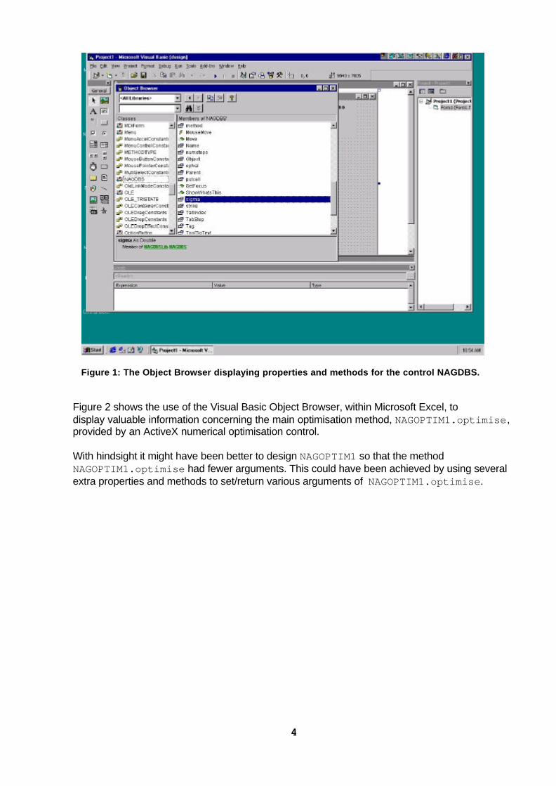
As is the case for all Microsoft controls, the properties and methods of each control can bedetermined interactively by using the Microsoft Object Browser, Figure 1. This information canbe very helpful when writing code that needs to know the arguments for a particular methodsupported by the control.

4

Figure 1: The Object Browser displaying properties and methods for the control NAGDBS.

Figure 2 shows the use of the Visual Basic Object Browser, within Microsoft Excel, todisplay valuable information concerning the main optimisation method, NAGOPTIM1.optimise,provided by an ActiveX numerical optimisation control.

With hindsight it might have been better to design NAGOPTIM1 so that the methodNAGOPTIM1.optimise had fewer arguments. This could have been achieved by using severalextra properties and methods to set/return various arguments of NAGOPTIM1.optimise.

5

Figure 2: Argument list information being supplied for the method NAGOPTIM1.optimise

3.1 The Fourier Transform Control

This example illustrates the use of an ActiveX control embedded in a Microsoft Word document.The control was created using Visual Basic and uses a NAG C Library routine [5], containedwithin a DLL, to perform the fast Fourier transform (FFT) of a given input sequence. It iscontained in the file NAG_FFT.ocx and has an associated Help file which explains how to usethe control.

The control was constructed using the following standard Microsoft ActiveX components: aVisual Basic form, textboxes and command buttons. Since this control contains several other(visible) ActiveX controls it cannot really be referred to as a (visually) primitive ActiveXcomponent. This means that it would not be suitable as a general purpose mathematicalcomponent which could be incorporated into an application that has its own custom interface.

The visual appearance of the control within the Word document is shown in Figure 3. Thesentence "The ActiveX control below uses … " is Word document text and does not form part ofthe control.

6

Figure 3: The fast Fourier transform control within a Word document.

3.1.1 Interactive Interface

The interactive use of the control is illustrated in Figure 4. A sequence of real numbers is inputand the fast Fourier transform is returned by clicking the Calculate button with the user'smouse.

Note: The control contains some Visual Basic code to display the results using complexnumber (<a, b>) notation.

Figure 4: Demonstration calculations using the Fourier transform control.

7

This particular ActiveX control has a Help button which when clicked displays a customisedHelp file. Figure 5 shows Help information on the use of the fast Fourier transform control withinan HTML Web page.

Figure 5: Help file information on the use of the fast Fourier transform control.

3.1.2 Language Interface

None was programmed. All the data input is done interactively.

3.2 The Financial Derivative Control

This control was created using Visual C++ and solves the Black-Scholes i.e., equation ([6], [7],[8]), using a variety of methods. It contains all of its own code and does not reference theNAG C Library DLL. The control is contained in the file NAGDBS.ocx, and its Visual Basicname in this example is NAGDBS1.


The interactive interface includes Property values that can be set using the MicrosoftProperties Window and also Events. Figure 6 shows how the background colour of the controlcan be set interactively at design time.

8

Figure 6: Selecting the background colour of the control at design time.

Here the ActiveX control uses an event to initiate computation. No calculations areperformed until the control has been clicked by the mouse, Figure 7.

Figure 7: The user form and control before computations are performed.

Once the control has been clicked the subroutine NAGDBS1_Click() is invoked andcomputations are performed; the source code within NAGDBS1_Click() is given below inSection 3.2.2.

9


When the control NAGDBS1 is placed on the user's form, Visual Basic will automaticallyprovide the following template code:

Private Sub NAGDBS1_Click()

End Sub

This subroutine is run whenever the control NAGDBS1 is clicked by the user's mouse. Herethe subroutine contains the following code:

Private Sub NAGDBS1_Click()

Dim greeks(3) As Double Dim T As Double Dim i As Long Dim opt_val As Double

NAGDBS1.putcall = 1 ' a put NAGDBS1.curval = 10# NAGDBS1.strike = 8# NAGDBS1.dividends = 0.06 NAGDBS1.method = 0 ' use standard lattice NAGDBS1.numsteps = 10 NAGDBS1.intrate = 0.1 NAGDBS1.sigma = 0.3

Print "AMERICAN PUT OPTIONS (USING CONTROL VARIATE)" Print " " NAGDBS1.extype = 2 ' american control variate Print " Time Option Value Delta Gamma Theta" Print "(Years)"

For i = 1 To 3 T = i * 0.25 NAGDBS1.maturity = T NAGDBS1.Calculate opt_val = NAGDBS1.optval NAGDBS1.greeks greeks(0) Print " "; Format(T, "#0.00"), Format(opt_val, "#0.0000"), _ Format(greeks(0), "#0.0000"), Format(greeks(1), "#0.0000"), _ Format(greeks(2), "#0.0000") Next i

End Sub

It can be seen that the properties NAGDBS1.putcall, NAGDBS1.curval, NAGDBS1.sigma,etc are used to set up the values for the problem. The method NAGDBS1.calculate is thenused to perform the required calculations, and option values and greeks are returned via theproperty NAGDBS1.optval and method NAGDBS1.greeks respectively. The effect of themouse click event is shown in Figure 8.

10

Figure 8: The user form after the derivative calculations have been performed.

3.3 The Optimisation Control

This control was created using Visual C++. The control is contained in the file NAGOPTIM.ocx,and its Visual Basic name in this example is NAGOPTIM1.

It illustrates the use of ActiveX to overcome the inability of the Visual Basic within Excel tosupply a user-defined function as an argument to a DLL routine. Mathematical routines thatrequire this feature include Quadrature, Ordinary Differential Equations, Partial DifferentialEquations, and Optimisation. The example considered here makes use of a nonlinearoptimisation routine, chosen because it is widely used and has a rather complicated interface.

It should be mentioned that rewriting the NAG routine so that it uses reverse communication isone way to overcome the user-defined function argument problem [9]. The COM methodoutlined here has the advantage that it leaves existing code unchanged and merely provides an"extra layer" of code to support the ActiveX interface.


No interactive features have been written for this control.


The example considered here was written to perform numerical optimisation on the datacontained within an Excel spreadsheet. An excerpt from the Visual Basic code is given below.

Private Sub Command1_Click()

Dim x() As Double Dim objname As String * 200 . . . n = Cells(1, 2).Value ncnlin = Cells(3, 2).Value

ReDim x(n)

11

ReDim bu(n + ncnlin) . . . x(0) = Cells(11, 2).Value . . . bu(6) = Cells(9, 4).Value

' set the objective and constraint function names objname = "my_objfun" constrname = "my_confun"

full_objname = ActiveWorkbook.Name & "!" & objname full_constrname = ActiveWorkbook.Name & "!" & constrname

NAGOPTIM1.pfunname "printit" NAGOPTIM1.ofunname full_objname NAGOPTIM1.cfunname full_constrname NAGOPTIM1.optimise n, nclin, ncnlin, a(0), tda, g(0), x(0), bl(0), bu(0) ' output the results Cells(13, 2).Value = x(0) Cells(13, 3).Value = x(1) Cells(13, 4).Value = x(2) Cells(13, 5).Value = x(3)

End Sub

The control provides methods which allow the user to specify the names of the objectivefunction, the constraint function and the print function that are to be used in the numericaloptimisation. Here the objective function was called my_objfun, the constraint functionmy_confun and the print function printit. Figure 9 shows the appearance of the Excelspreadsheet before the numerical optimisation has been performed. When the commandbutton labelled Solve is clicked the Visual Basic subroutine Command1_click() is run andthe input data, such as the number of variables and the upper and lower constraints, are readfrom the spreadsheet.

Figure 9: The Excel spreadsheet before the optimisation has been performed.

These values are then assigned to internal Visual Basic arrays and are passed to the controlNAGOPTIM1. The optimisation is then performed and the optimal values x(0)...x(3) areoutput to the Excel worksheet, Figure 10.

The objective function and constraint function are easily defined below.

12

The objective function is

Sub my_objfun(num_variables As Long)

' Any valid visual basic code is allowed here objective_value = x(0) * x(3) * (x(0) + x(1) + x(2)) + x(2)

End Sub

and the user-defined constraint function is

Sub my_confun(num_variables As Long, num_constraints As Long)

' Any valid visual basic code is allowed here constraint_value(0) = x(0) + x(1) + x(2) + x(num_variables - 1) constraint_value(1) = x(0) * x(0) + x(1) * x(1) + x(2) * x(2) + x(3) * x(3) constraint_value(2) = x(0) * x(1) * x(2) * x(num_variables - 1)

End Sub

The user-defined print function is considered in the following section.

It should be mentioned, for completeness, that this example contained a small amount of VisualBasic housekeeping code. Its purpose was to communicate the values of theobjective_value and the three element array constraint_value to the optimisationcontrol.

Figure 10: The Excel spreadsheet after the optimisation has been performed.

3.3.3 User-defined Print Function

Monitoring how an optimisation program is proceeding can be a problem from within Windows.The usual approach is to write the output to a file for later display. However, this method does not allow the user to display the monitoring information programmatically.

13

In this example the ActiveX control NAGOPTIM1 has been constructed to use the ExcelVisual Basic subroutine printit for the output of monitoring information. The subroutineprintit has twelve arguments and these can be used to display monitoring informationconcerning the number of iterations, the value of the objective function, the intermediatesolution vectors, etc.

The user has the flexibility of writing any valid Visual Basic code within printit to displaythese values. Here all the information was simply displayed within Excel Sheet3; this is shownin Figure 11.

The print function is as follows:

Sub printit(n As Long, it_maj_prt As Long, sol_prt As Long, maj As Long, mnr As Long, _ step As Double, nfun As Long, merit As Double, violtn As Double, norm_gz As Double,_ cond_hz As Double, x_ptr As Long)

Dim xp() As Double

With Sheets("Sheet3") If Row = 1 Then ' first call so output the headers Row = Row + 2 .Cells(Row, 1).Value = " Major" . . . End If If sol_prt Then ReDim xp(n) Call get_darray(x_ptr, xp(0), n) Row = Row + 2 .Cells(Row, 1).Value = "The optimal values of the variables are :" Row = Row + 2 For i = 0 To n - 1 .Cells(Row, 1 + i).Value = xp(i) Next i End If If it_maj_prt Then .Cells(Row, 1).Value = maj . . . Row = Row + 1 End If' End WithEnd Sub

Figure 11: An Excel spreadsheet with intermediate optimisation output.

14

Although the numerical optimisation example described here is fairly simple the same approachcan be used to solve much more complicated problems. This is illustrated in the next sectionwhere an optical optimisation problem is considered.

4 Internet Computing

Another application of ActiveX technology is the construction of components for active Webpages. In this section a ray tracing example will be considered which demonstrates calling anumerical optimisation component from within a Web page.

All the ActiveX controls mentioned here were written using Visual C++ and accessed viaVBScript programs.

4.1 Ray Tracing Example

This example plots the path taken by a ray of light in a non-uniform refractive medium.There is a choice of three different colours and a non-uniformity (decay) parameter can also beselected. It illustrates how mathematical ActiveX controls, based on NAG routines, can be usedto create scientific applications for the Internet.

The Web page is constructed using three customised ActiveX components and standardMicrosoft controls such as command buttons, labels and textboxes. The three customisedActiveX components are

• A nonlinear optimisation control, Nagoptd31• A graphical plotting control, Plot1• An integration control, NagIntg21

The ray tracing problem is modelled by finding the path which has the minimum optical pathlength, i.e., the minimum path integral of the product the distance with the (frequencydependent) refractive index. In this model the light path is assumed to follow a general cubiccurve, which means that there are only four unknown coefficients to be determined. Theproblem is solved by using the numerical integration control in conjunction with the nonlinearnumerical optimisation control. Two user-defined functions are therefore required: a user-defined objective function for the numerical optimisation and a user-defined integrand for thenumerical integration. This results in the call to the integration control, NagIntg21, beingnested within the objective function of the optimisation control, Nagoptd31.

The Web page before any calculations have been performed is shown in Figure 12.

Excerpts from the main VBScript program are now given. The properties and methods of eachcontrol will not be discussed in detail, since these can be worked out from the context in whichthey occur in the VBScript code.

4.1.1 The VBScript controlling the selection of the light colour

Sub CommandButtonBlue_Click() red_color = 0 green_color = 0 blue_color = 255 frequency = 7.0End Sub

Here the frequency and RGB plot colour is set to that corresponding to blue light when thecommand button labelled Blue is clicked.

15

4.1.2 The VBScript for the main calculation

Sub CommandButton1_Click() Dim bl(100) Dim bu(100) Dim loc_x(100) Dim g(100) . . . n = 3 num_vars = n num_pts = 51 canvas_height = 400 x_start = canvas_width - 500 y_start = canvas_height - 40

if (first_call = 1) then Plot1.BrushColor 11,224,230 Plot1.PenColor 0,0,0 Plot1.PenWidth = 3 Plot1.text "Fig 1. ActiveX Demonstration (Author: George Levy) ",x_start, y_start+20

Plot1.Rectangle x_start,20,x_start+337,y_start Plot1.circle 468,y_start,10 first_call = 0 Plot1.clear end if

i = 0 For i = 0 To 3 y_shift = i For k = 0 To num_vars - 1 bl(k) = -10.0 bu(k) = 10.0 Next bl(num_vars) = -y_shift bu(num_vars) = -y_shift

tda = 3 a(0) = 2.5 * 2.5 * 2.5 a(1) = 2.5 * 2.5 a(2) = 2.5

decay_factor = TextBox1.Value Nagoptd31.optimise n, nclin, ncnlin, a(0), tda, g(0), loc_x(0), bl(0), bu(0) Nagoptd31.getvars loc_x(0), n dx = 0.050 x_pos(0) = 0.0 xtemp = 0.0 For j = 0 To 50 y_pos(j) = loc_x(0) * x_pos(j) * x_pos(j) * x_pos(j) + loc_x(1) * x_pos(j) * x_pos(j) + loc_x(2) * x_pos(j) + y_shift xtemp = xtemp + dx y_pos(j) = y_pos(j) x_pos(j+1) = xtemp . . . do_plot()

NextEnd Sub

In this section of code the various plot characteristics are set: size of the plot region,background colour of plot region, pen width for plotting and also text/symbols for inclusionwithin the plot region. The results from the optimisation control Nagoptd31 are used tocalculate the ray trajectory, which is then plotted by a call to the VBScript subroutinedo_plot().

16

4.1.3 The VBScript for plotting the output

Sub do_plot() Plot1.PenColor red_color,green_color,blue_color Plot1.PenWidth = 2 Plot1.Getdata num_pts, x_pos(0), y_pos(0)End Sub

In this subroutine the colour and pen width used by the plot control Plot1 are set before theray's path is plotted.

Figure 12: The Web page before any calculations have been performed.

The user-defined objective function for the numerical optimisation is

Sub Nagoptd31_Objfunction() Dim x(100) Dim obj_val . . . num_vars = 3 obj_val = Nagoptd31.Objval Nagoptd31.getvars x(0), num_vars numintervals = 10 a = 0.0 b = 2.5 For i = 0 To num_vars - 1 params(i) = x(i) Next NagIntg21.integrate a, b, numintervals val = NagIntg21.answer obj_val = val Nagoptd31.Objval = obj_val Nagoptd31.setvars x(0), num_varsEnd Sub

Here the path integral between a = 0 and b = 2.5 is calculated using ten intervals.The answer is returned by the property NagIntg21.answer and this is set equal tothe value of the objective function Nagoptd31.objval.

17

The user-defined integrand for the numerical integration routine is

Sub NagIntg21_Integrand() Dim y Dim x . . . x = NagIntg21.getx n_o = 10.0 * (1.0 - 0.1 * frequency) y = params(0) * x * x * x + params(1) * x * x + params(2) * x + y_shift . . . opt_path = rindex * Sqr(temp) value = opt_path NagIntg21.getfunval = valueEnd Sub

The integrand takes into account both the frequency dependence (caused by dispersion) andthe spatial variation (caused by density) of the refractive index. The current example assumesthat the density of the medium is symmetrically distributed about the centre of the white ball onthe lower edge of the plotting region in Figure13. This is achieved by making the density at anypoint proportional to both the radial distance from the centre of the white ball and also a userspecified decay factor.

Figure 13: The Web page with the ray tracing results.

The results of the ray tracing are shown in Figure 13. Those interested in optical effects willrecognise this light bending as similar to mirage effects (where the air temperature alters therefractive index).

It should be mentioned that it would be easy, within a Web browser, to edit the user-definedintegrand (within the source of the Web page) so as to model different spatial distributions ofthe refractive index, or even change the optimisation and plot settings to model completely newproblems.

18

5 Inprise Delphi

The purpose of this section is to show how numeric ActiveX components can be incorporated into InpriseDelphi applications. The examples chosen here use the Financial Derivative andOptimisation controls previously described in Section 3. Since Delphi is similar to Visual Basiconly brief details will be given. However, the complete Delphi source is supplied in theAppendix and can be compared with the equivalent Visual Basic (VBScript) code given inSection 3.

5.1 Derivative Pricing Control

Views of the Delphi project at design time and run time are shown in Figure 14 and Figure 15respectively.

Excerpts from the Delphi source code are given below.

procedure TForm1.FormClick(Sender: TObject);var greeks: Array[1..5] of double; T: double; i: integer; opt_val: double; num_precision: integer; num_digits: integer; pos: integer; val1: String;begin NAGDBS2.putcall := 1; NAGDBS2.curval := 10.0; . . . num_digits := 4; Canvas.Brush.Color := clBtnFace; Canvas.TextOut(10,80,'AMERICAN PUT OPTIONS (USING CONTROL VARIATE)'); . . . Canvas.TextOut(400,140,'Gamma'); Canvas.TextOut(550,140,'Theta'); for i := 1 To 3 Do Begin T := i*0.25; . . . NAGDBS2.maturity := T; NAGDBS2.Calculate; NAGDBS2.greeks(greeks[1]); opt_val := NAGDBS2.optval; val1 := FloatToStrF(T,ffFixed,num_precision,num_digits); Canvas.TextOut(10,pos,val1); val1 := FloatToStrF(opt_val,ffFixed,num_precision,num_digits); . . .End;end;

19

Figure 14: The Delphi application with the derivative control NAGDBS2 on TForm1.

Figure 15: The Delphi application with the derivative control's results.

20

5.2 Optimisation Control

Views of the Delphi project at design time and run time are shown in Figure 16 and Figure 17respectively.

Excerpts from the Delphi source code are given below.

procedure TForm1.FormClick(Sender: TObject);var x:Array[0..40] of double; bl:Array[0..40] of double; bu:Array[0..40] of double; loc_x:Array[0..40] of double; g:Array[0..40] of double; a:Array[0..40] of double; . . .begin num1 := 4; darray[0] := 1.23; darray[1] := 3.456; n := 4; tda := 0; nclin := 0; bu[6] := 1000.0; . . . NAGOPTD21.optimise(n,nclin,ncnlin,a[0],tda,g[0],loc_x[0],bl[0],bu[0]); num_precision := 18; num_digits := 4; val1 := FloatToStrF(loc_x[0],ffFixed,num_precision,num_digits); Canvas.TextOut(20,300,val1); . . . val1 := FloatToStrF(loc_x[3],ffFixed,num_precision,num_digits); Canvas.TextOut(170,300,val1);end;

procedure TForm1.NAGOPTD21Objfunction(Sender: TObject);var obj_val:double;begin obj_val := NAGOPTD21.Objval; NAGOPTD21.getvars(x[0],num_vars); obj_val := x[0]*x[3]*(x[0]+x[1]+x[2])+x[2]; NAGOPTD21.setvars(x[0],num_vars); NAGOPTD21.Objval := obj_val;end;

procedure TForm1.NAGOPTD21Constrfunction(Sender: TObject);begin NAGOPTD21.getvars(x[0],num_vars); NAGOPTD21.getconstr(constraint_value[0],num_cons); constraint_value[0] := x[0]+x[1]+x[2]+x[num_vars-1]; constraint_value[1] := x[0]*x[0]+x[1]*x[1]+x[2]*x[2]+x[3]*x[3]; constraint_value[2] := x[0]*x[1]*x[2]*x[num_vars-1]; NAGOPTD21.setconstr(constraint_value[0],num_cons); NAGOPTD21.setvars(x[0],num_vars);end;procedure TForm1.FormCreate(Sender: TObject);beginend;end.

21

Figure 16: The Delphi application with the optimisation control NAGOPTD21 on TForm1.

Figure 17: The Delphi application with the optimisation control's results.

22

6 Conclusions

This paper has discussed the use of numeric ActiveX component software with primitive visualinterfaces. It has demonstrated that these software components are flexible and can easily beincorporated into (and removed from) existing applications using drag and drop techniques.These (usually invisible) numeric components are therefore the ideal computational engines ofapplications which have sophisticated user interfaces.

Since ActiveX component technology is based on C++, calls to complicated NAG routines canbe simplified through the use of properties, methods, events, object initialisation viaconstructors, data/information hiding within the object, and also optional arguments that takedefault values.

ActiveX components can be used by the entire range of Microsoft products, from PowerPoint toInternet Web browsers, and also by other Windows products such as Inprise Delphi.

The benefits to be gained through using numeric ActiveX components suggest that thistechnology will be increasingly used for mathematical computing instead of existing DLLmethods. However, the precise design of an individual component will still depend on theprogrammer's judgement.

23

7 References

[1] G F Levy (1998) Calling 32-bit NAG C DLL functions from Visual Basic 5 andMicrosoft Office, NAG Technical Report, TR2/98, NAG Ltd, Oxford.

[2] Inprise Corporation (1998) Delphi 4, Inprise Corporation.

[3] Microsoft Corporation (1997) Visual Basic 5, Component Tools Guide, Microsoft Corporation.

[4] D Kruglinski, G Shepherd and S Wingo (1998) Programming Microsoft Visual C++,Microsoft Press.

[5] NAG Ltd (1998) The NAG C Library, Mark 5, NAG Ltd, Oxford.

[6] F Black and M Scholes (1973) The Pricing of Corporate Liabilities, Journal of Political Economy81 637-657.

[7] G F Levy (1998) NAG Financial Routines, NAG Technical Report, TR3/98,NAG Ltd, Oxford.

[8] J Hull (1997) Options Futures and Other Derivatives, Prentice Hall.

[9] D Sayers (1999) Private Communication, NAG Ltd, Oxford.

24

8 Appendix

This Appendix contains the complete Delphi code for the examples given in Section 5.

8.1 Derivative Pricing Control

The complete Delphi source code for this example is given below.

unit Unit1;

interface

uses Windows, Messages, SysUtils, Classes, Graphics, Controls, Forms, Dialogs, StdCtrls, OleCtrls, NAGDBSLib_TLB;

type TForm1 = class(TForm) NAGDBS2: TNAGDBS; procedure NAGDBS2Click(Sender: TObject); procedure FormClick(Sender: TObject); procedure FormCreate(Sender: TObject); private { Private declarations } public { Public declarations } end;

var Form1: TForm1;

implementation

{$R *.DFM}

procedure TForm1.FormClick(Sender: TObject);var greeks: Array[1..5] of double; T: double; i: integer; opt_val: double; num_precision: integer; num_digits: integer; pos: integer; val1: String;begin NAGDBS2.putcall := 1; NAGDBS2.curval := 10.0; NAGDBS2.strike := 8.0; NAGDBS2.dividends := 0.06; NAGDBS2.method := 0; NAGDBS2.extype := 2; NAGDBS2.numsteps := 10; NAGDBS2.intrate := 0.1; NAGDBS2.sigma := 0.3; NAGDBS2.maturity := 0.25; NAGDBS2.Calculate; num_precision := 18; num_digits := 4; Canvas.Brush.Color := clBtnFace;

Canvas.TextOut(10,80,'AMERICAN PUT OPTIONS (USING CONTROL VARIATE)');

Canvas.TextOut(10,140,'Time'); Canvas.TextOut(10,160,'(Years)');

Canvas.TextOut(100,140,'Option Value'); Canvas.TextOut(250,140,'Delta'); Canvas.TextOut(400,140,'Gamma'); Canvas.TextOut(550,140,'Theta');

for i := 1 To 3 Do Begin T := i*0.25;

25

pos := i*30+160; NAGDBS2.maturity := T; NAGDBS2.Calculate; NAGDBS2.greeks(greeks[1]); opt_val := NAGDBS2.optval; val1 := FloatToStrF(T,ffFixed,num_precision,num_digits); Canvas.TextOut(10,pos,val1); val1 := FloatToStrF(opt_val,ffFixed,num_precision,num_digits); Canvas.TextOut(100,pos,val1); val1 := FloatToStrF(greeks[1],ffFixed,num_precision,num_digits); Canvas.TextOut(250,pos,val1); val1 := FloatToStrF(greeks[2],ffFixed,num_precision,num_digits); Canvas.TextOut(400,pos,val1); val1 := FloatToStrF(greeks[3],ffFixed,num_precision,num_digits); Canvas.TextOut(550,pos,val1); End;end;

procedure TForm1.FormCreate(Sender: TObject);begin

end;

end.

8.2 Optimisation Control

The complete Delphi source code for this example is given below.

unit Unit1;interfaceuses Windows, Messages, SysUtils, Classes, Graphics, Controls, Forms, Dialogs, OleCtrls, NAGOPTD2Lib_TLB;type TForm1 = class(TForm) NAGOPTD21: TNAGOPTD2; procedure FormClick(Sender: TObject); procedure NAGOPTD21Objfunction(Sender: TObject); procedure NAGOPTD21Constrfunction(Sender: TObject); procedure FormCreate(Sender: TObject); private { Private declarations } public { Public declarations } num1:integer; darray:Array[0..20] of double; constraint_value:Array[0..40] of double; x:Array[0..40] of double; Row:integer; num_vars:integer; num_cons:integer; end;var Form1: TForm1;implementation{$R *.DFM}procedure TForm1.FormClick(Sender: TObject);var x:Array[0..40] of double; bl:Array[0..40] of double; bu:Array[0..40] of double; loc_x:Array[0..40] of double; g:Array[0..40] of double; a:Array[0..40] of double; n:integer; ncnlin:integer; nclin:integer; tda:integer; constraint_value:Array[0..40] of double; num_precision:integer; num_digits:integer; val1:String;begin num1 := 4; darray[0] := 1.23; darray[1] := 3.456;

26

n := 4; tda := 0; nclin := 0; ncnlin := 3; num_vars := n; num_cons := ncnlin; loc_x[0] := 1.0; loc_x[1] := 1.0; loc_x[2] := 1.0; loc_x[3] := 1.0; bl[0] := 1.0; bl[1] := 1.0; bl[2] := 1.0; bl[3] := 1.0; bl[4] := -1000.0; bl[5] := -1000.0; bl[6] := 25.0; bu[0] := 5.0; bu[1] := 5.0; bu[2] := 5.0; bu[3] := 5.0; bu[4] := 20.0; bu[5] := 40.0; bu[6] := 1000.0; NAGOPTD21.optimise(n,nclin,ncnlin,a[0],tda,g[0],loc_x[0],bl[0],bu[0]); num_precision := 18; num_digits := 4; val1 := FloatToStrF(loc_x[0],ffFixed,num_precision,num_digits); Canvas.TextOut(20,300,val1); val1 := FloatToStrF(loc_x[1],ffFixed,num_precision,num_digits); Canvas.TextOut(70,300,val1); val1 := FloatToStrF(loc_x[2],ffFixed,num_precision,num_digits); Canvas.TextOut(120,300,val1); val1 := FloatToStrF(loc_x[3],ffFixed,num_precision,num_digits); Canvas.TextOut(170,300,val1);end;procedure TForm1.NAGOPTD21Objfunction(Sender: TObject);var obj_val:double;begin obj_val := NAGOPTD21.Objval; NAGOPTD21.getvars(x[0],num_vars); obj_val := x[0]*x[3]*(x[0]+x[1]+x[2])+x[2]; NAGOPTD21.setvars(x[0],num_vars); NAGOPTD21.Objval := obj_val;end;procedure TForm1.NAGOPTD21Constrfunction(Sender: TObject);begin NAGOPTD21.getvars(x[0],num_vars); NAGOPTD21.getconstr(constraint_value[0],num_cons); constraint_value[0] := x[0]+x[1]+x[2]+x[num_vars-1]; constraint_value[1] := x[0]*x[0]+x[1]*x[1]+x[2]*x[2]+x[3]*x[3]; constraint_value[2] := x[0]*x[1]*x[2]*x[num_vars-1]; NAGOPTD21.setconstr(constraint_value[0],num_cons); NAGOPTD21.setvars(x[0],num_vars);end;procedure TForm1.FormCreate(Sender: TObject);beginend;end.

numeric activex components - nag.com · numeric activex components g f levy nag ltd, wilkinson...

Documents