numerical algorithms for the direct spectral transform ...ilya/papers/comp_phys98.pdfshabat spectral...

JOURNAL OF COMPUTATIONAL PHYSICS147,166–186 (1998)ARTICLE NO. CP986087

Numerical Algorithms for the Direct SpectralTransform with Applications to Nonlinear

Schrodinger Type Systems

S. Burtsev,∗,1 R. Camassa,∗ and I. Timofeyev†,2∗Theoretical Division and Center for Nonlinear Studies, Los Alamos National Laboratory, Los Alamos,

New Mexico 87545;†Department of Mathematical Sciences, RPI, Troy, New York 12180-3590E-mail: [email protected], [email protected]

Received March 11, 1998; revised August 14, 1998

We implement two different algorithms for computing numerically the directZakharov–Shabat eigenvalue problem on the infinite line. The first algorithm replacesthe potential in the eigenvalue problem by a piecewise-constant approximation, whichallows one to solve analytically the corresponding ordinary differential equation.The resulting algorithm is of second order in the step size. The second algorithmuses the fourth-order Runge–Kutta method. We test and compare the performance ofthese two algorithms on three exactly solvable potentials. We find that even thoughthe Runge–Kutta method is of higher order, this extra accuracy can be lost becauseof the additional dependence of its numerical error on the eigenvalue. This limits theusefulness of the Runge–Kutta algorithm to a region inside the unit circle around theorigin in the complex plane of the eigenvalues. For the computation of the continu-ous spectrum density, this limitation is particularly severe, as revealed by the spectraldecomposition of theL2-norm of a solution to the nonlinear Schr¨odinger equation.We show that no such limitations exist for the piecewise-constant algorithm. In par-ticular, this scheme converges uniformly for both continuous and discrete spectrumcomponents. c© 1998 Academic Press

Key Words:nonlinear Schr¨odinger equation; Zakharov–Shabat eigenvalue prob-lem; nonlinear optics.

1. INTRODUCTION

The discovery and development of the soliton theory [1, 2] has had deep repercussionsin physics and applied mathematics. This theory has made possible the explicit integration

1 Present address: Corning Inc., Corning, NY 14831.2 To whom correspondence should be addressed at present address: Courant Institute of Mathematical Sciences,

251 Mercer Street, New York, New York 10012. E-mail: [email protected].

166

0021-9991/98 $25.00Copyright c© 1998 by Academic PressAll rights of reproduction in any form reserved.

DIRECT SPECTRAL TRANSFORM 167

of several partial differential equations (PDEs) with universal applicability. In particular,these equations were linearized via an associated linear system, the Lax pair, and explicitlyintegrated in the following sense: First, rich classes of exact solutions, infinite hierarchiesof conservation laws, and infinite-dimensional analogs of the action-angle variables werederived. Second, the solution of the Cauchy problem on the infinite line was recast in theform of a solvable linear integral equation, and the asymptotic nature of its solutions wasdetermined explicitly.

Two main ingredients in the solution of the Cauchy problem for integrable nonlinearpartial differential equations are the direct spectral transform and its inverse counterpart.These are nonlinear analogs of the direct and inverse Fourier transforms, respectively. Theyboth involve a single linear system of ordinary differential equations with a free (spectral)parameter and, in general, are not tractable analytically. Hence, in order to solve them, onehas to resort to numerical solvers.

Simple and effective PDE-solvers, developed in recent years, have made the numericalstudy of nonlinear wave phenomena in one spatial dimension relatively straightforward.Nevertheless, “raw” numerical modeling is still prohibitively time-consuming when onehas to map out multidimensional parameter spaces. Moreover, even an accurate and com-prehensive numerical simulation stops short of providing a fundamental understanding ofany nonlinear wave phenomenon.

In the special case of near-integrable partial differential equations, fundamental under-standing can be provided by decomposing the wave field into “normal” coordinates, i.e.,the soliton and nonsoliton components, also termed as the nonlinear spectral data. Sucha decomposition can be readily achieved by inserting the numerical solution of a givennear-integrable partial differential equation into a direct spectral transform solver. Apartfrom its intrinsic value, this decomposition can be useful for verifying and complementingperturbation calculations that describe the “flow” of the spectral data. To do this one has toanalyze snapshots of the potential for different times. These and other reasons (see [3]) ne-cessitate the development of efficient high-quality numerical solvers for the direct spectraltransform.

In this paper we concentrate on the nonlinear Schr¨odinger (NLS) equation

iqz+ 1

2qtt + q∗q2 = P, (1)

which describes propagation of light pulses in an optical fiber with the anomalous1 group-velocity dispersion [4, 5]. Here, we prefer to use the optical notation in which the normalizedtime t plays the role of a spatial coordinate and the normalized distancez plays the roleof a time-like coordinate, whileq(t, z) is the complex envelope of the electric field. TheperturbationP is specified by the particular physical problem at hand. WhenP= 0, theNLS system is integrable. The linearization of the NLS system is achieved by recasting thissystem as the Zakharov–Shabat spectral problem [6], which is a system of two ODEs for

1 The case of normal group-velocity dispersion leads to a similar equation with only a change of the relativesigns of the terms on the left-hand side of (1). In this case the associated spectral problem is self-adjoint and,hence, somewhat simpler to treat.

168 BURTSEV, CAMASSA, AND TIMOFEYEV

the scalar wave functionsφ1 andφ2,

dφ1

dt= qφ2− i ζφ1,

dφ2

dt= −q∗φ1+ i ζφ2,

(2)

whereζ is an eigenvalue parameter. By using the Zakharov–Shabat spectral problem, incombination with the appropriately chosen linear ODEs which define thez-evolution ofφ1

andφ2, one can also solve analytically several other important nonlinear partial differentialequations. Besides the nonlinear Schr¨odinger equation, which is currently receiving a greatdeal of attention due to its technological applications in fiber optics, these partial differentialequations include the Maxwell–Bloch system, the sine–Gordon equation, the usual and themodified Korteveg–de Vries equations, etc.

In this paper, we present an efficient numerical algorithm for solving the direct Zakharov–Shabat spectral problem. We have incorporated this numerical algorithm in a code thatcomputes the flow of the spectral data and in particular eigenvalues, for the perturbed NLSequation (1). For this application, we optimize the performance of the eigenvalue-searchalgorithm by using our knowledge of the history of the spectral data. Our code is able tospeed up the search for each eigenvalue in subsequent snapshots of the perturbed NLSsolution by a factor of 5, provided that the number of eigenvalues does not change from onesnapshot of the solution to another.

The main focus of this work is to describe and compare two different algorithms forsolving Zakharov–Shabat spectral problem, which differ by how one solves the system ofordinary differential equations (2) withζ as a parameter. The first approach [3] replacesthe potentialq with its piecewise-constant approximation. This allows us to solve thecorresponding ODE analytically. The second approach [7] proposes using a high-orderODE integrator, such as a fourth-order Runge–Kutta scheme. Both algorithms use a grid-search approach to find the eigenvalues. We have tested both methods on a variety ofexplicitly solvable potentials: soliton, oversoliton, and a rectangular potential. One of themost important findings that emerges from our study is that only the piecewise-constantalgorithm is effective computing the continuous spectrum contribution to theL2-norm (theconserved “number of particles” functional) of solutions of the unperturbed NLS equation.

The numerical error in the Runge–Kutta approach cannot be controlled uniformly overthe spectrum. Specifically, the Runge–Kutta’s local truncation error depends on the eigen-value asζ 4, which limits its applicability to the unit circle region around the origin of thecomplexζ plane. This limitation is dramatically revealed by the spectral decomposition ofthe L2-norm of solutions of the NLS equation. Our tests show that for a given discretiza-tion step the error in computing the continuous spectrum contribution to theL2-norm bythe Runge–Kutta method can be over an order of magnitude larger than the error of thepiecewise-constant method.

The layout of this paper is the following. In Section 2, we recall a few basics of the solitontheory. The properties of the spectral problem depend heavily on the type of boundaryconditions, i.e., an infinite-line problem with the potentialq(t) decaying at infinity or at-periodic problem for the potentialq(t). In this paper we only investigate the infinite lineproblem. In Section 3, we introduce both solvers: Runge–Kutta and piecewise-constant,and describe our implementation of the eigenvalue-search algorithm. In Section 4, we


present the results of the error analysis. The test results are given in Section 5. Finally, inSection 6, we illustrate the performance of the eigenvalue solver, based on a piecewise-constant approximation and the eigenvalue search algorithm by applying it to a realisticfiber-optic problem:Non-return-to-zeroto soliton data conversion in the optical line withsliding frequency guiding filters [8, 9].

2. THE DIRECT AND INVERSE SPECTRAL TRANSFORMS

When the perturbationP is absent, Eq. (1) is equivalent to the overdetermined linear sys-tem for a vector-valued wave functionΦ = (φ1, φ2)

T (with (·, ·)T denoting the transpose),

Φt +UΦ = 0, (3)

Φz+ VΦ = 0, (4)

where 2× 2 matrix functionsU andV and the two-dimensional (column) vector functionΦ depend on the timet , the coordinatez, and the spectral parameterζ in the followingfashion:

U = i ζσ3+ u,

V = i ζ 2σ3+ ζu+ v − i ζ 2I .

Here,

σ3 =(

1 00 −1

), I =

(1 00 1

),

u =(

0 −qq∗ 0

), v = i

2

(−|q|2 −qt

−q∗t |q|2).

The functionq(t, z) is the wave field of the unperturbed NLS equation, and the system (3)is nothing but the scalar system (2) rewritten in a vector form. The compatibility conditionUz−Vt +VU−U V = 0 between Eqs. (3) and (4) is exactly the unperturbed NLS system.

Let us recall a few properties of the system pair (3) and (4). Equation (3) has the structureof an eigenvalue problem with the complex parameterζ (the Zakharov–Shabat spectral prob-lem [6]). This problem can be thought of as a nonlinear analog of the Fourier transform forlinear problems. Generically, an initial conditionq(t, 0) gives rise to a continuous spectrumrepresented by a functionr (ζ ), with each real-valuedζ being the analog of the frequencyof a dispersive wave component. In addition to the continuous spectrum, the Zakharov–Shabat spectral problem supports a discrete spectrum, whose corresponding modes haveno counterpart in the Fourier transform. This discrete spectrum consists of complex pairs{ζk= ξk + iηk, ρk}, k= 1, . . . , N, whereN is the number of solitons which will emergefrom the initial data for sufficiently largez. The properties of these solitons are determinedby ζk andρk as follows: for eachk, the real part of the complex eigenvalueζk, ξk=Re(ζk)

equals one half of the corresponding soliton frequency, and the imaginary partηk= Im(ζk)

equals one half of the soliton amplitude; the complex coefficientρk parameterizes the soli-ton’s initial position and its complex phase. In the limit of infinitely smallq, the discretespectrum is absent and the continuous spectrum coincides with the spectral density of linearFourier harmonics.


To present theSpectral Data={r (ζ ), ζ ∈ R; ζk, ρk, k= 1, N} in greater detail, we needto recall a few extra elements of the Zakharov–Shabat spectral problem. We begin with thecontinuous spectrum, represented by the functionr (ζ ) when the eigenvalueζ is locatedon the real axis. First, we introduce the vector solutionsΦ1 andΦ2 (the Jost functions) ofsystems (3) and (4),

Φ1 =(

10

)exp(−i ζ t)[1+ o(1)], t →−∞,

Φ2 =(

0−1

)exp(i ζ t)[1+ o(1)], t →−∞,

(5)

fixed by their asymptotics at the left endt→−∞. Hence, for each pointζ of the continuousspectrum one finds two independent solutionsΦ1,2. We also need the solutionsΨ1 andΨ2

fixed by their asymptotics at the right end,

Ψ1 =(

10

)exp(−i ζ t)[1+ o(1)], t →∞,

Ψ2 =(

01

)exp(i ζ t)[1+ o(1)], t →∞.

(6)

Out of these vector solutionsΦ1,2 andΨ1,2, one can construct two different fundamentalmatrix solutions8= (Φ1,Φ2) and9 = (Ψ1,Ψ2) which are related to each other via ascattering matrixS

8 = 9S, S=(

a b∗

b −a∗

). (7)

The functionr (ζ ) is the ratio of the elements of the scattering matrixS: r (ζ )= b(ζ )/a(ζ ).By using the relation (7), one derives useful formulas which are valid for real values of thespectral parameterζ ,

a(ζ ) = limt→∞φ1(t, ζ )exp(i ζ t),

b(ζ ) = limt→∞φ2(t, ζ )exp(−i ζ t),

(8)

where the scalar functionsφ1,2 are the components of the vector-valued Jost functionΦ1.Due to the fact that the Zakharov–Shabat spectral problem is not self-adjoint, the corre-

sponding eigenvaluesζk are complex-valued. Each eigenvalue is located in the upper halfζ -plane, and its corresponding Jost function is fixed by its asymptotics at the left end,

Φ1k =(

10

)exp(−i ζkt)[1+ o(1)], t→−∞.

The asymptotics of the Jost functionΦ1k on the right end is parameterized by normalizationconstantbk,

Φ1k = bk

(01

)exp(i ζkt)[1+ o(1)], t→∞.


The coefficientρk is expressed in terms ofbk andζ -derivativea′k of the spectral coefficientaat the position of the eigenvalueζk: ρk= bk/a′k. We assume that a potentialq(t) is sufficientlysmooth and that it vanishes at|t |→∞ fast enough so that the discrete spectrum containsa finite number of eigenvalues. We also assume that each zero ofa is a simple one. Themappingq(t)→Spectral Datamakes up the direct spectral problem. The solution of theinverse mapping may be reduced to a linear integral equation of Volterra type (Gelfand–Levitan–Marchenko system) [1, 2].

For the unperturbed NLS equation the evolution of the spectral data inzcan be computedusing Eq. (4). By substituting the evolved spectral data into the Gelfand–Levitan–Marchenkosystem one can determine the solutionq(t, z) at anyz> 0. The essential point that makesthis procedure possible is that the spectral data evolve inz in a trivial manner for any initialfunctionq(t, 0):

dζk/dz= 0,

dρk/dz= 2i ζ 2k ρk,

dr(ζ, z)/dz= 2i ζ 2r.

For instance, in the case of an initial condition with discrete spectrum only (r (ζ )= 0), onecan write down an explicit solution that describesN interacting solitons. In the simplestcase of a single soliton,N= 1, we have a familiar sech-shaped pulse:

qs = 2ηeiφ

cosh(2ηθ),

θ = t + 2ξz− t0, (9)

φ = −2ξ(t + 2ξz)+ 2i (η2+ ξ2)z+ φ0,

2ηt0= ln[|ρ(z= 0)|/(2η)], φ0 = π − arg[ρ(z= 0)]. (10)

Conservation laws for the NLS system can be expressed either in terms of the potentialq(t, z) or in terms of the spectral data. The simplest of the conserved quantities is theL2-norm ofq, the so-called “number of particles.” This norm can be written as

∫ ∞−∞|q(t, z)|2 dt = − 1

π

∫ ∞−∞

ln|a(ξ)|2 dξ +N∑

k=1

2i (ζ ∗k − ζk), (11)

which shows explicitly how the continuous and discrete spectra contribute to theL2-normof the potentialq. In the following we will often refer to this norm simply as the energyof q, and to the first term on the right-hand side of (11) as the continuous spectrum (ordispersive waves) energy.

In the presence of a general perturbationP, it is not known how to introduce an evolutionequation (4) so that the perturbed NLS again arises as the compatibility condition betweentwo linear systems, analogous to equations (3) and (4). Thus, the evolution equation of thespectral data inz cannot be derived, and hence, the solution cannot be reconstructed forz> 0. If the perturbationP is small enough, one can find approximate evolution equationsfor the spectral data via asymptotic expansions. However, these equations will become


invalid after some distancez, typically corresponding to a drastic change in the discretespectrum when a soliton component vanishes or a new one is generated.

The decomposition into soliton and dispersive components, given by the spectral problem(3), is a valuable alternative to the Fourier transform, because this decomposition providesan efficient way of storing information about the solution. For instance, in the unperturbedcase, one soliton mode can replace an infinite number of Fourier components. Moreover, forsmall perturbations, we can use the decomposition into soliton and dispersive componentsof the initial conditionq(t, 0) and the unperturbed equation to predict the dynamics of theperturbed solution on finitez-intervals. Of course, this is only true for small perturbationsP; for largeP’s there is no a priori argument why the nonlinear Fourier transform shouldbe superior to the linear Fourier transform.

3. NUMERICAL DISCRETIZATION

In this section, we introduce two distinct algorithms for solving the direct Zakharov–Shabat spectral problem. Even though the Zakharov–Shabat spectral problem is defined onthe infinitet-line, we have to truncate the potential outside a sufficiently large interval forboth algorithms, in order to make its numerical solution possible. As a result, the infinite-line spectral problem is reduced to a problem with a compactly supported potential, and thecorresponding boundary conditions can be moved from the±∞ to the boundaries of thetruncated potential.

The solution of the spectral problem begins by integrating the system of ordinary differ-ential equations (3) withζ as a complex parameter. The major difference between the twoalgorithms lies in the way they solve this ODE system. The piecewise-constant approxi-mation utilizes the fact that we can solve the linear ODE system (3) analytically wheneverthe potentialq(t, z) is constant. Since the potentialq is discretized on the grid with a timestep1t , one possible approach is to assume that the potential is constant on each subinter-val (tn−1t/2, tn+1t/2) and solve the direct Zakharov–Shabat problem exactly on eachsubinterval using matrix exponentials.

It is possible to improve the piecewise-constant algorithm by assuming a higher orderapproximation for the potentialq (i.e., piecewise-linear). In this case one still can solve theODE system (3) analytically. The disadvantage of this approach is caused by the necessityto use Airy functions in order to express the solution of the ODE system, which leads to adramatic increase in the computational cost.

High-order numerical integration of the ODE system (3) presents an alternative to theapproximate analytical solution. We choose to use the fourth-order Runge–Kutta method[10] as the simplest representative of the high-order ODE solvers.

3.1. Piecewise-Constant Approximation

In this subsection we recall the fundamentals of the piecewise-constant approximationfor the Zakharov–Shabat spectral problem [3]. The potentialq(t) is truncated outside asufficiently large interval (−L , L). Inside this interval,q(t) is chosen to be equal to a constantqn=q(tn) on each elementary subinterval (tn−1t/2, tn+1t/2), where the pointtn equals−L + n1t . Here, the time step1t equals1t = L/M , with the 2M+1 being the total numberof discretization points of the interval (−L , L). As a result, the corresponding ODE (3)can be solved exactly inside each elementary subinterval for any value of the spectral


parameterζ . The corresponding solution readsΦ(tn+1t/2, ζ )= T(qn, ζ )Φ(tn−1t/2, ζ ),whereΦ(tn−1t/2, ζ ) is the “initial” condition on the left end of the elementary subintervaland the transfer matrixT(qn, ζ ) is the exponential of the matrixU (qn, ζ ):

T(qn, ζ ) = exp[−1tU (qn, ζ )] = exp

[1t

(−i ζ qn

−q∗n i ζ

)]

=(

cosh(κ1t)− i ζκ−1sinh(κ1t) qnκ−1sinh(κ1t)

−q∗nκ−1sinh(κ1t) cosh(κ1t)+ i ζκ−1sinh(κ1t)

).

The parameterκ, given by the equationκ2=−|qn|2−ζ 2, is constant inside each interval1t .In order to solve the scattering problem we have to “propagate” the solution using the

transfer matrixT(qn, ζ ) from−L to L. The final result is

Φ(L −1t/2, ζ ) = 5Φ(−L −1t/2, ζ ), (12)

where

5(ζ) =2M∏n=1

T(qn, ζ ) (13)

is obtained by the ordered multiplication of all transfer matrices. The unknown spectralcoefficientsa(ζ ) andb(ζ ) can be explicitly expressed in terms of the values of the JostfunctionΦ1 on the “right” end ast→∞ from (8). By taking the initial condition

Φ(−L −1t/2, ζ ) =(

10

)ei ζ(L+1t/2) (14)

in Eq. (12), we express the value of the Jost functionΦ1 on the “right” end in terms ofthe matrix function5. On the other hand, we know a priori that this value generates thecoefficientsa andb,

Φ1(L −1t/2, ζ ) =(

a(ζ )ei ζ(−L+1t/2)

b(ζ )ei ζ(L−1t/2)

)

and, therefore,

a(ζ ) = 511(ζ )e2i ζ L ,

b(ζ ) = 521(ζ )ei ζ1t .(15)

To obtain the normalization coefficientsρk, we also have to be able to compute thederivative ofa(ζ ) with respect toζ . Differentiation of the expression (15) fora(ζ ) leads to

da

dζ= 2i La(ζ )+ e2i ζ L d

dζ

(511(ζ )

). (16)

The last term in this expression contains the derivative with respect toζ of 511(ζ ), thefirst entry in the matrix from the ordered product (13). Differentiation yields a sum overthe partial products that form5(ζ) timesζ -derivatives of the matrixT(qn, ζ ). This sumcan be computed within the same iteration loop that produces the ordered product5, withminimal extra cost.


3.2. Fourth-Order Runge–Kutta Method

We have also implemented a fourth-order Runge–Kutta algorithm as an alternative tothe piecewise-constant approximation. In this case, the matrixU (q, ζ ) serves the role ofa known variable coefficient. By switching from the wave functionΦ= (φ1, φ2)

T to itsenvelopeχ= (χ1, χ2)

T,

Φ = (φ1 = χ1 e−i ζ t , φ2 = χ2 ei ζ t)T, (17)

we eliminate the fast oscillations which arise when Re(ζ ) is large and obtain the followingequations for the slowly varying functionsχ1,2:

d

dtχ1 = qχ2e2i ζ t ,

d

dtχ2 = −q∗χ1e−2i ζ t .

(18)

The computation of the coefficientsa andb via the Runge–Kutta approach is analogousto the same computation via the piecewise-constant approximation. As a result, we need totake special initial conditions att =−L for (χ1, χ2)

T= (1, 0)T. Finally, by calculating thevalue of the vector functionχ on the “right” end, we obtain the coefficientsa andb as(

a(ζ )

b(ζ )

)=(χ1(L , ζ )

χ2(L , ζ )

).

To compute the derivative ofa(ζ ) obtained with the Runge–Kutta algorithm, we found thatan efficient and accurate method is provided by the Romberg algorithm [12].

3.3. Search for Eigenvalues

Once we know how to solve the ODE system (3) for any value of the spectral pa-rameterζ , we can proceed to the solution of the Zakharov–Shabat spectral problem. Thenumerical computation of the continuous spectrum, defined by the reflection coefficientr (ζ )=a(ζ )/b(ζ )with ζ on the real axis, follows from Eq. (15) or (3.2) in a straightforwardfashion. The localization of the discrete eigenvaluesζk, located in the upper half of thecomplexζ -plane, is not trivial. To find them, we use the facts that the coefficienta(ζ ) canbe analytically continued into the upper halfζ -plane from the real axis and that the discreteeigenvalues coincide with the complex zeros ofa(ζ ) which we assumed to be simple.

First, following [3], we observe that the total numberN of eigenvalues may be computedby calculating the total phase shift ofa(ζ ) on the real axis from the “left” end ofζ -axisto the “right”: N= arg(a(ζ ))|∞−∞/(2iπ). Being one-dimensional, this calculation can beperformed using a fineζ grid for maximum accuracy. Second, we implement the gridsearch for the eigenvaluesζk by computing the values of 1/a(ζ ) on a sufficiently large gridwith preassigned grid size. The grid points at which the value of 1/a(ζ ) exceeds a certainpractical limit serve as candidates for the eigenvalues. These candidates are tested by tryingto further approximate them by using the secant method. Knowledge of the total numberNof the discrete eigenvalues indicates whether we have found all of them or not. If we misssome of the eigenvalues, we repeat the search on a refined grid.


We notice that the problem of finding the eigenvalues with small imaginary parts requiresspecial care. This problem is important from a practical point of view because these smalleigenvalues may naturally appear during the “birth” or “death” of a soliton. We paid specialattention to this problem while implementing the search algorithm.

Another possible approach to the eigenvalue search is to compute a contour integral of thefunction ofa′/a over some closed path in the complexζ plane. Sincea(ζ ) is analytic, thisintegral will give the number of eigenvalues inside the contour. This technique can be usedfor both the calculation of the total number of eigenvalues and their localization. We haveencountered significant problems during the numerical implementation of this approach.The first problem is caused by the necessity to compute the derivative ofa(ζ ). This increasesthe computation time, in fact drastically so in the case of the Runge–Kutta algorithm.Another, and more serious, limitation of this contour-integral approach is generated by thesensitivity of the above formula when the eigenvalue is located too close to the contour ofintegration, which requires a rather complicated adaptive algorithm for selecting the pathof integration.

4. ERROR ESTIMATES

4.1. Error for Piecewise-Constant Approximation

To estimate the numerical error for the piecewise-constant approximation, one can useperturbation results obtained for the Zakharov–Shabat spectral problem (see, e.g., [13]).According to this approach, the piecewise-constant approximate potentialqpwc is noth-ing but the perturbed exact potential:qpwc=q+ δq. The error in the coefficienta(ζ ) isexpressed in terms of an integral over the perturbationδq of the potential, and the functionsφ1,2 andψ1,2 which are components of the corresponding unperturbed Jost vector functionsΦ1 (5) andΨ2 (6):

δa =∞∫

−∞dt(δqφ1ψ1+ δq∗φ2ψ2). (19)

For the purposes of the error analysis it is sufficient to consider only the first term in theexpression (19). The second term can be estimated in a similar fashion. Using the shorthandnotation f =φ1ψ1, we can rewrite the error caused by the first term as

∫∞−∞ δq f dt.

To estimate the error contribution1a= ∫ 1t/2−1t/2 δq f dt added on the elementary subin-

terval (−1t/2,1t/2), we representδq asδq=q(t)− q(0) and expandf andq in Taylorseries. As a result, we obtain

1a =(1t

2

)3 1

3[ f q′′ + 2 f ′q′] + O((1t)4), (20)

where ′ = d/dt. The fact that we choose the grid point in the middle of the elementarysubinterval is essential for obtaining(1t)3—dependence for the local error1a. By summingup the local errors1a over the whole interval (−L , L) we obtain that the global error ina(ζ ) is proportional to(1t)2.

The complex spectral parameterζ so far has been hidden in the error estimate fora,which is valid for any value ofζ . To analyze theζ -dependence of the errorδa, we need to


look at the expression (20) more closely. By using the asymptotic expression for the vectorJost functions at largeζ ,

Φ1 ∼(

10

)exp(−i ζ t)[1+ o(1)], ζ→∞, (21)

Ψ2 ∼(

01

)exp(i ζ t)[1+ o(1)], ζ→∞, (22)

we obtain f, d f/dt ∼ ζ−1. Thus, at large values ofζ

δa ∼ 1t2

ζ.

Therefore, the global numerical error in the coefficienta(ζ ) decreases withζ which is incontrast with the case for the Runge-Kutta case presented below, where the correspondingerror increases beyond all bounds asζ→∞.

The second-order global numerical error for the coefficienta(ζ ) translates into an errorof the same order for the eigenvaluesζk. An additional source of error during the numericalcomputation of the eigenvaluesζk is created by the iteration process in the secant method.This additional error is controlled by finding the zeros ofa with high precision. Therefore,the total error in the eigenvalues is kept at second order in1t .

The numerical error for the coefficientb is estimated in a similar way. It is also of secondorder in1t .

4.2. Error for Runge–Kutta Method

An estimate of the local truncation error for the Runge–Kutta method can be found in astandard fashion [10, 11]. The exact solutionΦ= (φ1, φ2)

T satisfies system (2).The approximate solutionΦ(a)

n = (φ(a)1n, φ

(a)2n)T, n= 0, 1, 2, . . ., satisfies the difference

equation (DE)

Φ(a)n+1=Φ(a)

n +1tG(Φ(a)

n ,q; ζ), (23)

with the functionG(Φ(a)n ,q; ζ ) given by

G(Φ(a)

n ,q; ζ) = 1

6(k1+ 2k2+ 2k3+ k4),

where thek’s are given by the usual Runge–Kutta iterations of the (linear) functionF(Φ,q; ζ ) at the right-hand side of system (2), starting withk1=F(Φ,q; ζ ). The localtruncation error,

τ (t0) ≡ Φ(t0+1t)−Φ(t0)1t

−G(Φ(t0),q(t0); ζ )

on the elementary subintervalt ∈ (t0, t0+1t), has a standard representation

τ =CF(I V ) · (1t)4, F(I V ) = d4

dt4F

∣∣∣∣t=t0+θ21t

, 0< θ < 1. (24)


From Eq. (23) (see [11]) it follows that the global discretization error|Φ(tn)−Φ(a)n | ∼ τ .

Also, by differentiating the functionF as in formula (24) four times, we derive that the localtruncation error has a fifth-order dependence onζ : τ ∼ ζ 5 due to the presence of the termsi ζφ1 and i ζφ2 in F. Moreover, this fifth-order dependence accumulates even in regionswhere the potentialq is identically zero.

To improve the accuracy of the Runge–Kutta approach, we make the change of variables(17) by switching from the wave function itself to its envelopeχ . As a result, the transformedright-hand side of Eq. (18) no longer has a term linear inζ , and the oscillatory term exp(2i ζ t)is restricted to the support of the potentialq. Therefore, the local truncation errorτ for theRunge–Kutta discretization of Eq. (18) is proportional to the fourth power ofζ . Moreover,the proportionality coefficient is nonzero only on the support ofq.

Note that the local truncation errorτ causes corresponding errors for all the computedspectral characteristics, such as the discrete eigenvalues and the continuous spectrum (seeFig. 1 and the tables in Section 5).

We will test these error estimates in the next section. For noncompact support potentialsqwe always use a sufficiently large interval (−L , L), so that the error generated by neglectingthe potential outside this finite domain is negligible, compared with the local error of anyof the two integration methods.

5. TESTS

We have implemented both the piecewise-constant approximation and the fourth-orderRunge–Kutta algorithms in Fortran 77. We have performed a series of tests on a SiliconGraphics workstation under the operating system IRIX64 release 6.1 with the R8000 75 MHzprocessor. All computations were done in double precision. To illustrate the performance ofthe program we present the CPU time for the one-soliton potential. The CPU time dependson a variety of parameters: on the number of points used for the discretization, on thenumber of discrete eigenvalues, and their position in the complexζ -plane.

5.1. One-Soliton Potential

First, we consider the simplest possible case, namely, a one-soliton potential (10), whosespectrum is known exactly. We have chosen the soliton parameters so that the correspondingeigenvalueζ equals1

2(1+ i ) and the normalization coefficientb/a′ equals−i . As a result,the one-soliton potential equalsq(t)= exp(−i t )/cosh(t). For the “pure” soliton potential,there is no continuous spectrum.

The numerical results for this soliton potential, presented in Tables I and II, demonstratethat for this particular case all the spectral data (the discrete eigenvalue, the normalizationcoefficient, and the continuous spectrum) are found with good accuracy. The “Cont. Sp.En.” column in Table I denotes the numerical value of the continuous spectrum (dispersivewaves) contribution to theL2-norm ofq, calculated from formula (11). Figure 1 shows thatour implementations of the Runge–Kutta and piecewise-constant approximation methodsare of fourth order and second order in time step, respectively. This result agrees with theanalytical error estimates derived in Section 4.

Note that Table II, unlike Table I, does not have the “Continuous Spectrum Energy”column. The reason for this is that the Runge–Kutta method produces an error of order onewhen it calculates this parameter.


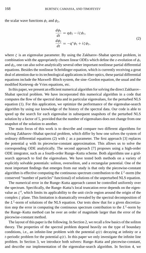
TABLE I

The Spectrum of a One-Soliton Potential Obtained by Using

the Piecewise-Constant Algorithm

Points 1t Discr. Eigenvalue Cont. Sp. En. Norm. Coeff.

128 0.3125 0.49725+ i 0.49460 1.7E-02 1.2E-04− i 0.98927256 0.1562 0.49931+ i 0.49864 3.3E-03 5.4E-06− i 0.99728512 0.0781 0.49983+ i 0.49966 1.2E-07 1.9E-06− i 0.99931

1024 0.0391 0.49995+ i 0.49991 7.9E-09 −5.6E-07− i 0.999822048 0.0195 0.49998+ i 0.49997 4.9E-10 −3.9E-06− i 0.99994

Exact 0.5+ i 0.5 0 −i

We also provide a comparison of the CPU time that each algorithm takes to completethe task of finding the one-soliton spectrum of Tables I and II. The Runge–Kutta-basedalgorithm is roughly 20–30% faster than the piecewise-constant method for this particulartask. In general, over all the tests we have conducted, the two algorithms’ speeds wereroughly the same. Of course, the running time for both algorithms is architecture-dependentand the CPU times we present (obtained on the IRIX workstation) are meant to give thereader an idea about the cost of the computations in this particular case (see Table III). Thetwo algorithms share the same routines for the eigenvalue search in the complex plane, andin both cases most of the CPU time is spent by the procedure which locates the discreteeigenvalues in the complexζ plane. In particular, in the test for one-soliton potential bothalgorithms spend over 80% of their time searching for the zero ofa(ζ ). The majority oftime during the search is spent on computing the values ofa(ζ ) on the grid.

We stress that the time for locating the eigenvalues depends considerably on their posi-tion in the complexζ plane. We implemented an algorithm which starts the search for theeigenvalues from the imaginary axis and then propagates to the left and to the right simulta-neously. Therefore, the time spent for locating the eigenvalues is proportional to amplitudesof their real parts. The coefficient of proportionality depends on the grid spacing and thenumber of nodes in the grid.

5.2. Oversoliton

Our next test aims at checking how accurately both the piecewise-constant and Runge–Kutta approaches calculate a nonzero continuous spectrum. As a test potential we take

TABLE II

The Spectrum of a One-Soliton Potential, Obtained by Using the

Fourth-Order Runge–Kutta Approach

Points 1t Discr. Eigenvalue Norm. Coeff.

128 0.3125 0.499999990+ i 0.499270300 7.60E-08− i 0.99746220256 0.1562 0.499999990+ i 0.499949000 8.32E-08− i 0.99984100512 0.0781 0.499999990+ i 0.499996700 8.38E-08− i 0.99999000

1024 0.0391 0.499999990+ i 0.499999790 8.39E-08− i 0.999999302048 0.0195 0.499999997+ i 0.499999987 8.39E-08− i 0.99999996

Exact 0.5+ i 0.5 −i


FIG. 1. Error in the eigenvalueζ1 versus the number of discretization points for one-soliton potential (seeTables I and II).

q(t)= 2Aexp(−0.3t)/cosh(2t) (so-called oversoliton) where the parameterA must be cho-sen to be 1 for a “pure” soliton, but in our caseA may have any positive value. For such apotential, the Zakharov–Shabat scattering problem can be solved analytically for any valueof A [14]. In general, both the discrete and continuous spectra are present in the problem. Inthe case whenA= 1.4, there is a single eigenvalueζ1= 0.15+ 1.8i , plus a certain amountof nonzero continuous spectrum. We choose not to present the lengthy expressions for thecoefficientsa(ζ ) andb(ζ ) (see [14]). Out of the total pulse energyEtotal= 4A2= 7.84, thesoliton part isEsol= 4η= 7.2, while the rest of the energy is contained in the nonsolitoncomponent:Econt.spectr.= 0.64.

Tables IV and V contain the numerical results on the discrete spectrum plus the pulseenergy due to the nonsoliton component and illustrate that, with respect to the calculation ofthe continuous spectrum, the piecewise-constant approach is by far superior to the Runge–Kutta method.

TABLE III

CPU Time of Computations

Points Piecewise-constant Runge–Kutta

128 67 s 51 s256 135 s 102 s512 275 s 205 s

1024 573 s 409 s2048 1236 s 816 s


TABLE IV

Spectrum of the Oversoliton Potential:q(t) = 2A exp(−0.3t)/cosh(2t) with

A = 1.4, Obtained by Using a Piecewise-Constant Approximation

Points 1t Discr. eigenvalue Cont. Sp. En.

128 0.3125 0.146174+ i 1.778069 0.7126577256 0.1562 0.149087+ i 1.794385 0.6536514512 0.0781 0.149774+ i 1.798589 0.6399762

1024 0.0391 0.149943+ i 1.799647 0.63999302048 0.0195 0.149985+ i 1.799911 0.6399987

Exact 0.15+ i 1.8 0.64

In Table V we do not present data on the continuous spectrum energy because in all cases,except the case of 2048 points (1t = 0.0195), the Runge–Kutta method produces errors oforder 1.

5.3. Rectangular Potential

In the final test, we analyze the integrators’ performance in the case of discontinuouspotentials. We consider the rectangular potentialq(x)=q0, |x|< L. For such a potential,explicit formulas exist for the coefficientsa andb, which are

a(ζ ) = e2i ζ L

[cos(2νL)− i ζ

νsin(2νL)

], b(ζ ) = −q0

νsin(2νL),

where the parameterν is expressed in terms of the spectral parameterζ and the potentialamplitudeq0 in the formν2= ζ 2+ q2

0. In our test, we have chosen the following values forthe potential amplitudeq0 and the potential widthL: q0=−π/2, L = 1. The total energyin this case isπ2/2. To determine the eigenvalues, one has to look for the zeros of thecoefficienta(ζ ). As a result, one determines that the rectangular potential with the givenchoice of parameters leads to a single purely imaginary discrete eigenvalueζ1 ≈ 1.062572i .Hence, the energy of the continuous spectrum isEcont.spec. ≈ 0.6845133. The main differ-ence between this and the previous tests is that the potential is not smooth, which leadsto larger errors for both the piecewise-constant and Runge–Kutta methods. Notice thatin the case of the piecewise-constant method this error is caused solely by the need to

TABLE V

Spectrum of the oversoliton potential:q(t) = 2A exp(−0.3t)/

cosh(2t) with A = 1.4, Obtained by Using the Fourth-Order

Runge–Kutta Approach

Points 1t Discr. eigenvalue

256 0.1562 0.14999998+ i 1.790426512 0.0781 0.14999998+ i 1.799356

1024 0.0391 0.14999997+ i 1.7999592048 0.0195 0.14999997+ i 1.799997

Exact 0.15+ i 1.8


TABLE VI

Comparative Performance of Both the Piecewise-Constant Approximation

and the Fourth-Order Runge–Kutta Method

Points 1t Piecewise-Const. method Runge–Kutta method

128 0.3125 0.12205 0.46012256 0.1562 0.01897 0.19840512 0.0781 0.02746 0.20978

1024 0.0391 0.00467 0.042092048 0.0195 0.00707 0.01101

Note.The maximum error in the energy density of the continuous spectrum for the rectangularpotential.

evaluate the potential at the middle of the discretization step; with the proper discretiza-tion the piecewise-constant algorithm naturally yields an exact solution for the rectangularpotential.

The continuous spectrum energy is nonzero for the rectangular potential. In this test weanalyze not only the numerical errors incurred in the calculation of the integral charac-teristic, such as the total energy input by the continuous spectrum, but also the numeri-cal errors in the local characteristic—a measure of the intensity of the dispersive waves,supζ |(2/π) log|a(ζ )||, whereζ is on the real axis.

As expected, we can see that the piecewise-constant approximation performs much better,compared with the results of the fourth-order Runge-Kutta method (Table VI).

Finally, we present the numerical results for the full spectral data of the rectangularpotential (Tables VII and VIII).

The Runge–Kutta method computes the continuous radiation correctly only for1t =0.01953125 (2048 points). In all other cases, this method produces an error of order one.Moreover, the Runge–Kutta method completely fails for1t = 0.3125—the method in thiscase gives the wrong number of eigenvalues.

Our numerical results demonstrate that in the case of a rectangular potential, the conver-gence of all the spectral parameters is much slower, compared with the two previous tests.This is due to the discontinuity of the rectangular potential, which results in the fact that theerror estimates involving the derivatives of the potential, which we derived in the previoussection, are not quite valid.

TABLE VII

Spectrum of the Rectangular Potential Obtained by Using the

Piecewise-Constant Approximation

Points 1t Discr. eigenvalue Cont. Sp. En. Norm. Coeff.

128 0.3125 2.1E-09+ i 1.13409 0.836357 2.7E-08+ i 2.85167256 0.1562 2.4E-09+ i 1.07568 0.684812 2.1E-08+ i 2.39278512 0.0781 1.6E-09+ i 1.04187 0.627221 1.1E-08+ i 2.23392

1024 0.0391 5.8E-09+ i 1.05920 0.653978 4.5E-08+ i 2.276122048 0.0195 1.2E-09+ i 1.06755 0.668988 1.0E-08+ i 2.30095

Exact i 1.062572 0.6845133 i 2.283050


TABLE VIII

Spectrum of the Rectangular Potential Obtained by Using

the Fourth-Order Runge–Kutta Approach

Points 1t Discr. eigenvalue Norm. Coeff.

128 0.3125256 0.1562 4.68E-09+ i 1.055425 3.57E-08+ i 2.266125512 0.0781 5.37E-10+ i 1.030430 3.75E-09+ i 2.186588

1024 0.0391 1.02E-09+ i 1.064940 8.11E-09+ i 2.2913272048 0.0195 1.62E-09+ i 1.070325 1.32E-08+ i 2.309555

Exact i 1.062572 i 2.283050

We also remark that in our tests for the one-soliton potential and oversoliton, the Runge–Kutta algorithm finds the discrete spectrum eigenvalues with higher accuracy than thepiecewise-constant approximation. This is in accordance with our error analysis, since thetests’ eigenvalues are within or close to the unit circle (cf. Tables I and II, IV and V).Because of the discontinuity in the potential, this advantage of the Runge–Kutta method islost in the case of the rectangular potential (cf. Tables VII and VIII).

The results obtained in this section prove that, overall, the piecewise-constant approxima-tion is superior to the fourth-order Runge–Kutta method as a tool for finding the Zakharov–Shabat spectrum of the solutions to the NLS equation.

6. NON-RETURN-TO-ZERO TO SOLITON DATA CONVERSION PROBLEM

In this section, we illustrate the performance of our code utilizing the piecewise-constantapproximation on a light pulse propagation problem in nonlinear optical fibers.

A very simple and effective source of solution-like pulses in optical soliton transmissionexperiments was proposed and implemented recently [8]. The basic idea is to generate asoliton signal starting from a Non-return-to-zero (NRZ) source and imposing a subsequentsinusoidal phase modulation of each NRZ bit, where the modulation frequency is chosen tobe equal to the bit rate. If this signal is injected into a transmission line with sliding-frequencyguiding filters then, after a complicated transient evolution, localized soliton-like pulsesemerge (see Fig. 2, where for simplicity we consider the case of one single bit). Therefore,this phenomenon can be used to implement a method of converting NRZ bit streams into soli-ton signals. We consider an optical transmission line with periodically spaced, lumped am-plifiers, each followed by a Fabry–Perot filter whose peak frequencies are shifting (“sliding”)linearly with the distance along the line. When the dispersion length is much larger than theamplifier spacing, a good model for signal transmission is the “averaged,” normalized, NLS(1)[4, 15, 16] with the following perturbationP:

P = (i /2)[αq − β(i ∂t − ω f )2q]. (25)

This perturbation models the Fabry–Perot filter via the “Gaussian” approximation, whichis defined by three main parameters:β is the filter strength,α is the excess gain, whileω′f


FIG. 2. Conversion of a single NRZ-phase-modulated bit into a soliton in a transmission line with sliding-frequency guiding filters (numerical simulation).

parameterizes the sliding rate of the peak frequency of the filters,ω f , with the distance,

ω f = ω0+ ω′f z, (26)

whereω0 denotes the initial filter frequency offset from the carrier.The initial condition for Eqs. (1), (25), which we focus on, is the phase-modulated NRZ

signal

q0(t) = a(t) exp[iµ sin(Ät)], (27)

wherea(t) is the NRZ signal flipping between 0 andA. We have used the following practicalnormalized values of the system parameters for the present problemα= 0.4, β = 0.4, ω′f =0.185, Ä= 2π/8.82. The amplitudeA and the depth of phase modulationµ then can serveas the optimization parameters for the converted soliton-like pulse.

By applying our code to the initial pulse with the amplitudeA and the depth of phasemodulationµ chosen equal to 1 and 0.7π , respectively, we can clearly see that it is equiv-alent to four soliton eigenvalues:ζ1= 0.57+ 0.79i, ζ2=−0.56+ 0.15i, ζ3=−0.36+0.55i, ζ4=−0.1+ 0.54i , plus a small amount of dispersive waves (about 10% in terms ofthe total pulse energy). Thus, the initial pulse consists of the primary soliton eigenvalueζ1= 0.57+0.79i (the initial filter position coincides with the primary eigenvalue frequency:ξ1=Re(ζ1)), which gives rise to the output soliton, plus extra modes which are suppressedby the in-line filtering. Notice that while they are present, these additional componentsact like noise in the system and can lead to signal corruption by an uncontrollable shiftof the position of the primary soliton in its time slot. To provide an efficient conversionof the phase-modulated NRZ signal into solitons, it is therefore important to suppress thisnoise as early as possible during the transmission. A hybrid numerical–analytical approachwas proposed in [9] to analyze the conversion of an NRZ input to a soliton output signal in


FIG. 3. The trajectories of all eigenvalues detected in the initial condition (27) (based on the numericalsimulation of the full equation processed by the nonlinear spectral transform). Here,ξ is the eigenvalue frequencywith the sliding part being subtracted:ξ = ξ − ω′f z.

an optical line with sliding frequency guiding filters. The numerical part consists of apply-ing the nonlinear spectral transform solver to the input signal. This allows us to identify thesoliton modes in the signal and then to follow the evolution of each single soliton mode byapplying the adiabatic approximation.

Another possible approach is to compute the solution of the perturbed nonlinearSchrodinger equation (1) numerically with the NRZ signal as an initial condition and thento analyze snapshots of the solution using the spectral code to provide a clear picture ofhow the spectral data evolves in time. We illustrate the application of this approach to theexample above. Figure 3 presents the time evolution of the eigenvalues under the filteringperturbation (25). Only one (primary soliton) out of four survives. Here,ξ is the eigen-value frequency with the sliding part being subtracted:ξ = ξ − ω′f z. Note that our codeis sensitive enough to catch the emergence of a transient soliton, which was absent at thebeginning. In the unperturbed case, soliton and nonsoliton modes do not interact with eachother, but this is not so in the general perturbed case. When one of the secondary solitonsdisappears, it leaves behind a packet of dispersive waves. This wave packet can in turn startto accumulate enough energy which it eventually “sheds” in the form of a small-amplitudetransient soliton.

It is remarkable that, with the exception of these transient episodes, the results on the timeevolution of the eigenvalues obtained numerically with the help of the nonlinear spectraltransform are in good agreement with the the results predicted by the adiabatic approxi-mation. In fact, the availability of the nonlinear spectral code in this problem ultimatelyverifies (and extensively complements) the adiabatic approximation. Such a code helps inanswering basic questions, such as: “How close is the output pulse to a soliton of the unper-turbed NLS?” We calculate the amount of energy of the dispersive waves contained in theoutput pulse by using our code and can definitely say that for the given practical parameters,


the output pulse is an almost “pure” soliton. Only 2% of the total pulse energy is in thenonsoliton components when the conversion process is over.

7. CONCLUSIONS

In this work, we have implemented two different algorithms to compute numerically thedirect spectral transform (the direct Zakharov–Shabat eigenvalue problem on the infiniteline) which is used heavily in soliton theory and its applications in nonlinear fiber optics.The first algorithm uses a piecewise-constant approximation to the potential in order tosolve the corresponding ODE, and the second algorithm uses the fourth-order Runge–Kuttamethod.

We have tested and compared the performance of these two algorithms on three exactlysolvable potentials. We find that, despite the fact that the truncation error of the Runge–Kutta method is of higher order, the additional dependence of this error on the eigenvalues ofthe Zakharov–Shabat spectral problem limits the usefulness of the Runge–Kutta approach.Ultimately, this method can be effective only within the unit disk around the origin ofthe complex plane of the eigenvalues. This is a critical limitation when computing thenonsoliton part of the nonlinear spectrum, which can receive significant contributions fromintervals along the real axis far from the origin. Moreover, this additional dependenceposes restrictions on the class of potentials for which the discrete soliton spectrum can becomputed accurately. One example, which is important for signal analysis via nonlinearFourier transform, is that of a potentialq(t) which varies slowly int (and so the length2L for the ODE computation can be fairly large). From system (2), it is easy to showthrough a simple rescaling of time that this case is equivalent to one with a large amplitudepotential and a (rescaled) large eigenvalue parameter|ζ |. Thus, based on our error analysis,the Runge–Kutta method can be expected to lose accuracy in this case.

The limitation suffered by the Runge–Kutta method can be expected to affect any high-order ODE integrator. It is directly caused by the fact that the numerical truncation errorof the nth order method is proportional to thenth time derivative of the right-hand sideof the spectral ODE,F(n)(1t)n, whereF is the right-hand side of the ODE (18), and1tis the mesh size. Due to the presence of the spectral parameterζ in the ODE, one has|F(n)| ∼ ζ n, or ζ n+1, depending on which Eq. (18) or (3) is used. Therefore, any attempt toincrease the accuracy of the numerical solution by using a higher order numerical integratorautomatically fails as soon as|ζ | À 1. We have found that no such limitations exist forthe piecewise-constant approximation, and in fact, the truncation error for this methoddecreases, instead of increasing, with large|ζ | as |ζ |−1. Conversely, the truncation erroranalysis for higher order methods points to the fact that an efficient search for eigenvaluesnear the origin is most effectively carried out using a higher order method like Runge–Kutta.

In summary, our work shows that the piecewise-constant approximation algorithm is thebetter tool overall; it is the most robust and offers the same efficiency for the computationof both discrete and continuous spectra.

We have illustrated the performance of a code based on this algorithm by applying itto NRZ-to-soliton data conversion problem in a fiber-optical line with sliding frequency-guiding filters. One of the important features of our algorithm is the optimization of thesearch for eigenvalues in case of multiple snapshots of the potential. The NRZ-to-solitondata conversion problem provides an example where the flow of the spectral data in perturbedintegrable systems needs to be analyzed. This problem can be divided into two independent


tasks. First, the numerical solution of the perturbed equation is computed on a time gridof stepsizeδt . Second, a spectral code is utilized to analyze snapshots of the numericalsolution taken at timesδt apart. We make use of the fact that in most cases the spectral dataare orderδt close for two consecutive snapshots of the numerical solution, and therefore itis possible to use the spectral data computed for one snapshot of the potential as the initialguess for the spectral data of the next snapshot. This optimization of the search algorithmmakes a tremendous difference when there are eigenvalues with large (in absolute value)real parts. For example, we found that if there are eigenvalues with real parts greater than 0.5then the search is more than five times faster if the information from the previous snapshotof the potential is used. The optimized code is therefore especially valuable for trackingthe eigenvalues of potentials obtained as numerical simulations of perturbed integrableequations.

ACKNOWLEDGMENTS

The authors thank A. R. Osborne for his numerous stimulating remarks and E. A. Overman for helpful dis-cussion. S. Burtsev and R. Camassa acknowledge support from the U.S. Department of Energy under ContractW-7405-ENG-36 and the Applied Mathematical Sciences Contract KC-07-01-01. I. Timofeyev thanks the The-oretical Division and Center for Nonlinear Studies at the Los Alamos National Laboratory for their hospitalityand support during the summers of 1995 and 1996 and acknowledges support from the U.S. Department of En-ergy under Contract DE-FG02-93ER25154 and the National Science Foundation through the NSF TraineeshipDMS-9256302 and Grants DMS-9502142 and DMS-9510728.

REFERENCES

1. S. V. Manakov, S. P. Novikov, L. P. Pitaevskii, and V. E. Zakharov,Theory of Solitons(Consultants Bureau,New York, 1984).

2. M. J. Ablowitz and H. Segur,Solitons and the Inverse Scattering Transform(SIAM, Philadelphia, 1981).

3. G. Boffetta and A. R. Osborne, Computation of the direct scattering transform for the nonlinear Schr¨odingerequation,J. Comput. Phys.102, 252 (1992).

4. A. Hasegawa and Y. Kodama,Solitons in Optical Communication(Oxford Univ. Press, Oxford, 1995).

5. G. P. Agrawal,Nonlinear Fiber Optics, 2nd ed. (Academic Press, San Diego, 1994).

6. V. E. Zakharov and A. B. Shabat,Sov. Phys. JETP34, 62 (1972).

7. A. R. Bishop, M. G. Forest, D. W. McLaughlin, and E. A. Overman II, A quasiperiodic route to chaos in anear-integrable PDE. Spatio-temporal coherence and chaos in physical systems,Phys. D23(1–3), 293 (1986).

8. P. V. Mamyshev and L. F. Mollenauer,OFC’95 Technical Digest, 302 (1995).

9. S. Burtsev, R. Camassa, and P. Mamyshev,The NRZ-to-Soliton Data Conversion Problem, Los AlamosNational Lab Report LAUR 97-347 (1997).

10. W. H. Press, S. A. Teukolsky, W. T. Vetterling, and B. P. Flannery,Numerical Recipes, 2nd ed. (CambridgeUniv. Press, New York, 1992).

11. J. Stoer and R. Bulirsch,Introduction to Numerical Analysis(Springer-Verlag, New York/Berlin, 1991).

12. G. Engeln-Mullges and F. Uhlig,Numerical Algorithms with C(Springer-Verlag, New York/Berlin, 1996).

13. A. C. Newell, The inverse scattering transform, inSolitons, edited by R. K. Bullough and P. J. Caudrey(Spriner-Verlag, New York/Berlin, 1980).

14. J. Satsuma and N. Yajima, Initial value problem in one-dimensional self-modulation of nonlinear waves indispersive media,Progr. Theor. Phys.55, 284 (1974).

15. L. F. Mollenauer, J. P. Gordon, and S. G. Evangelides, The sliding-frequency guiding filter: An improvedform of soliton jitter control,Opt. Lett.17, 1575 (1992).

16. A. Hasegawa and Y. Kodama, Guiding-center soliton in optical fibers,Opt. Lett.15, 443 (1990). [Guiding-center soliton,Phys. Rev. Lett.66, 161 (1991)]

numerical algorithms for the direct spectral transform ...ilya/papers/comp_phys98.pdfshabat spectral...

Documents