numerical algorithms for tracking dynamic fluid-structure ... filebody-conforming computational...

Numerical Algorithms for Tracking Dynamic Fluid-StructureInterfaces in Embedded/Immersed Boundary Methods∗

Kevin Wang∗, Jon T. Gretarsson, and Alex MainInstitute for Computational and Mathematical Engineering,

Stanford University, Stanford, CA 94305, USA

In any embedded/immersed boundary method, the embedded/immersed boundary needs to be tracked withrespect to the non body-conforming Computational Fluid Dynamics (CFD) grid. When dealing with dynamicfluid-structure interaction problems with complex structural geometry, a robust, accurate, and efficient inter-face tracking algorithm becomes an important component of the computational framework. Existing methodsdeveloped in the CFD community have primarily focused on tracking closed boundaries with respect to uni-form or non-uniform Cartesian CFD grids. In this work, two robust and efficient algorithms are presentedfor tracking embedded/immersed fluid-structure interfaces with respect to three-dimensional, arbitrary (i.e.structured or unstructured) CFD grids. First, a projection-based approach can be used when the interface isclosed and fully resolved by the CFD grid, as it relies on the interface to separate the two distinct flow regimes“inside” and “outside” of it. When the surface is not closed, or is not fully resolved by the CFD grid, a slowerbut more general and accurate collision-based approach can be employed. Both approaches take advantage ofa bounding box hierarchy to efficiently store and access the elements of the discretized interface. Moreover,for distributed flow computations, an algorithm for constructing distributed bounding box hierarchies is alsopresented. The performances of these algorithms are assessed in three-dimensional, dynamic fluid-structureinteraction problems in the fields of aeronautics and underwater implosion. The differences between the twointerface tracking algorithms in terms of capability, accuracy, and efficiency are revealed and discussed.

I. Introduction

Debuted in 1972 for the fluid-structure interaction (FSI) simulation of blood flows around elastic heart valves,1

embedded/immersed boundary methods have been gaining popularity in the past four decades for simulations of bothflows around fixed obstacles2, 3, 7, 9 and dynamic FSI problems in which the structural motion/deformation can be eitherprescribed,4, 5, 11, 15 or computed by a computational structural dynamics (CSD) solver that is coupled in the simula-tion.1, 6, 8, 10, 13, 14 In this work we focus on methods designed for dynamic FSI problems, keeping in mind that they arealso applicable to flows around fixed obstacles. These methods can be attractive for two reasons. First, by using nonbody-conforming Computational Fluid Dynamics (CFD) grids, mesh generation is dramatically simplified, especiallywhen the structural wet surface has complex geometry. In fact, most methods in this category are actually designedto operate on Cartesian grids.1, 4–6, 8, 10, 11, 13, 15 More importantly, by using CFD grids that are fixed in time, meshmotion computations are totally avoided, which gives embedded/immersed boundary methods the capability of han-dling large structural motions and deformations1, 4–6, 8, 11, 14 or topological changes,10 for which alternative ArbitraryLagrangian-Eulerian (ALE) methods17–19 are unfeasible.

Despite the advantages outlined above, there are two major challenges for embedded/immersed boundary meth-ods. First, because the non body-conforming CFD grid does not have a native representation of the structural wetsurface, the discretization and imposition of fluid wall boundary conditions (addressed in [2–5, 7, 9, 11]) or fluid-structuretransmission conditions (addressed in [1, 6, 8, 10, 13, 14]) are not straightforward. To resolve this issue, various interfacetreatment techniques have been proposed in the past which involves modifying either the continuous governing equa-tions, or the discrete numerical scheme in the vicinity of the structural wet surface. A summary of these techniquesis provided in [15]. Second, at every time-step, the embedded/immersed structural wet surface must be tracked withrespect to the non body-conforming CFD grid using some computational tools. Indeed, every interface treatment tech-nique requires some information about the location of the structural wet surface with respect to the CFD grid. These∗Copyright c© 2011 by Kevin Wang. Published by the American Institute of Aeronautics and Astronautics, Inc., with permission.

1 of 21

American Institute of Aeronautics and Astronautics

computational tools must be robust, accurate, and time-efficient in order to handle embedded/immersed interfaces withcomplex geometry in refined grids.

The design and implementation of numerical algorithms for tracking in three-dimensional space the structural wetsurface (which is also the fluid-structure interface in FSI problems) is addressed in this paper. These algorithms take asinput the position and connectivity information of a non body-conforming CFD grid, as well as a Lagrangian surfacegrid representing the interface. Depending on the needs of the employed embedded/immersed boundary method, theoutput of these algorithms usually include some or all of the following types of information:

(1). Status of each grid-point of the CFD grid identifying the flow regime in which it resides.

(2). Location of the closest points on DEh to selected grid-points of the CFD grid in the vicinity of the interface.

(3). Location of intersection points where the edges of the CFD grid penetrates the interface.

Existing algorithms developed in the CFD community have primarily focused on tracking closed surfaces (e.g. surfaceof a solid body) with respect to uniform or non-uniform Cartesian CFD grids.3–5, 8, 11 Benefiting from the Cartesiangrid, (2) can be achieved easily and efficiently using geometric3–5, 5, 5, 11 or non-geometric8 Closest Point Transformalgorithms. Based on the assumption of closed surfaces, (1) is determined by inspecting the outward normal directionsof simplices in the vicinity of a given grid-point.3, 5, 11 Finally, intersection points are detected for penetrating edges,which are identified as edges in the CFD grid whose end-points reside in different flow regimes.4 It is notable that anedge that intersects the (closed) surface twice will not be considered as a penetrating edge as end-points reside in thesame flow regime. (See Figure 5, Case II.) This problem is very likely to occur when the structure is thin and not wellrefined by the CFD grid. (See Section IV.A.) For sharp interface treatment algorithms, this may lead to fluid “leaking”through the structure.14

In this paper, two robust and efficient approaches for tracking fluid-structure interfaces with respect to three-dimensional, arbitrary (i.e. structured or unstructured) CFD grids will be presented. Both algorithms are designed tobe capable of outputting (1),(2), and (3) discussed above. However, if some of them are not required by the employedinterface treatment method, certain steps can be skipped to avoid unnecessary computations. First, a projection-basedapproach (detailed in Section III.A) can be used when the interface is closed and fully resolved by the CFD grid,relying on the interface to separate the two distinct flow regimes “inside” and “outside” of it. When the structure is notclosed (e.g. a membrane sheet), or is not fully resolved by the CFD grid, such as when the structure is a thin airplanewing, a slower but more general and accurate collision-based approach, motivated by the methods proposed in [6, 12] inthe graphics community and detailed in Section III.A, can be employed. Both approaches take advantage of a boundingbox hierarchy21 to efficiently store and access the elements of the discrete interface. Moreover, for distributed flowcomputations, an algorithm for constructing distributed bounding box hierarchies (detailed in Section III.C is alsoproposed.

The performances of these proposed algorithms are assessed in three-dimensional, dynamic fluid-structure inter-action problems in the fields of aeronautics and underwater implosion. The differences between the two interfacetracking algorithms in terms of capability, accuracy, and efficiency are revealed and discussed.

II. Computational framework for fluid-structure interaction problems

A mathematical model for three-dimensional, dynamic fluid-structure interaction problems involves (1) the fluidgoverning equations within fluid domain ΩF(t)⊂R3; (2) the structural governing equations within structural domainΩS(t)⊂R3; (3) transmission conditions at the fluid-structure interface ΣE(t) = ΣF(t)∩ΣS(t), where ΣF(t) = ∂ΩF(t)and ΣS(t) = ∂ΩS(t) represent respectively the fluid and structural domain boundaries; (4) Dirichlet and/or Neumannboundary conditions at the remaining fluid and structural domain boundaries; and finally (5) initial conditions forfluid and structural variables at t = 0. Whereas the fluid and structural domains as well as the fluid-structure interfacevary in time, it is a general assumption in this work that the entire computational domain Ω = ΩF(t)∪ΩS(t) is time-independent. (See Figure 1.)

The choices of fluid and structural models and the formulations of their governing equations depend on the physicalproblems of interest. In this work, we assume that the fluid equations are formulated in a spatial (Eulerian) coordinatesystem while the structural equations are formulated in a material (Lagrangian) coordinate system. The chosen fluidand structural equations are coupled via appropriate transmission conditions. For example, [14] states that for aninviscid fluid and a flexible structure the corresponding velocity and equilibrium transmission conditions are

2 of 21


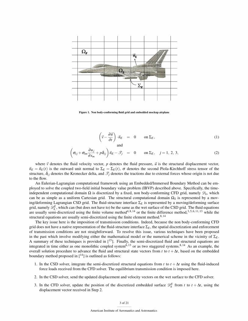
Figure 1. Non body-conforming fluid grid and embedded mockup airplane

(~v− ∂~u

∂ t

)·~nE = 0 on ΣE , (1)

and(σi j +σim

∂u j

∂xm+ pδi j

)~nE −T j = 0 on ΣE , j = 1, 2, 3, (2)

where ~v denotes the fluid velocity vector, p denotes the fluid pressure, ~u is the structural displacement vector,~nE = ~nE(t) is the outward unit normal to ΣE = ΣE(t), σ denotes the second Piola-Kirchhoff stress tensor of thestructure, δi j denotes the Kronecker delta, and T j denotes the tractions due to external forces whose origin is not dueto the flow.

An Eulerian-Lagrangian computational framework using an Embedded/Immersed Boundary Method can be em-ployed to solve the coupled two-field initial boundary value problem (IBVP) described above. Specifically, the time-independent computational domain Ω is discretized by a fixed, non body-conforming CFD grid, namely Dh, whichcan be as simple as a uniform Cartesian grid. The structural computational domain ΩS is represented by a mov-ing/deforming Lagrangian CSD grid. The fluid-structure interface ΣE is represented by a moving/deforming surfacegrid, namely DE

h , which can (but does not have to) be the same as the wet surface of the CSD grid. The fluid equationsare usually semi-discretized using the finite volume method4, 8, 14 or the finite difference method,3, 5, 6, 11, 13 while thestructural equations are usually semi-discretized using the finite element method.8, 14

The key issue here is the imposition of transmission conditions. Indeed, because the non body-conforming CFDgrid does not have a native representation of the fluid-structure interface ΣE , the spatial discretization and enforcementof transmission conditions are not straightforward. To resolve this issue, various techniques have been proposedin the past which involve modifying either the mathematical model or the numerical scheme in the vicinity of ΣE .A summary of these techniques is provided in [15]. Finally, the semi-discretized fluid and structural equations areintegrated in time either as one monolithic coupled system6, 13 or as two staggered systems.8, 14 As an example, theoverall solution procedure to advance the fluid and structural state vectors from t to t +∆t, based on the embeddedboundary method proposed in [14] is outlined as follows:

1. In the CSD solver, integrate the semi-discretized structural equations from t to t +∆t using the fluid-inducedforce loads received from the CFD solver. The equilibrium transmission condition is imposed here.

2. In the CSD solver, send the updated displacement and velocity vectors on the wet surface to the CFD solver.

3. In the CFD solver, update the position of the discretized embedded surface DEh from t to t + ∆t, using the

displacement vector received in Step 2.

3 of 21


4. In the CFD solver, track the discretized embedded surface DEh (t +∆t) with respect to the fixed, non body-

conforming CFD grid by collecting the following information:

4.1. status of each grid-point of the CFD grid, which determines whether or not it belongs to the fluid domain.

4.2. location of intersection points where the edges of the CFD grid penetrates DEh .

5. In the CFD solver, compute edge-based fluid fluxes by imposing the velocity transmission conditions. For eachedge (Vi,Vj) in CFD grid Dh which connects grid-points Vi and Vj:

5.1. if Vi and Vj both belong to fluid domain ΩF(t + ∆t), and edge (Vi,Vj) does not intersect DEh (t + ∆t),

compute the usual Roe20 flux between grid-points Vi and Vj.

5.2. if Vi and Vj both belong to fluid domain ΩF(t +∆t), and edge (Vi,Vj) intersects DEh (t +∆t), solve the

one-dimensional fluid-structure Riemann problem stated in Section 3 of [14] between each grid-point andthe interface, using the structural velocity. The resulting fluid state is used to compute a Roe flux for eachgrid-point.

5.3. if one of the two grid-points belong to fluid domain ΩF(t +∆t), (Vi,Vj) must intersect DEh (t +∆t). In

this case, solve the one-dimensional fluid-structure Riemann problem between the “active” grid-point andthe interface, using the structural velocity. The resulting fluid state is used to compute a Roe flux for the“active” grid-point.

5.4. if neither Vi nor Vj belongs to fluid domain ΩE(t +∆t), no computations are performed.

6. In the CFD solver, integrate the semi-discretized fluid equations from t to t +∆t.

7. In the CFD solver, integrate local fluid-induced force loads on a surrogate of DEh (See Section 4 and 5 of [14])

and distribute them onto intersection points. Then, redistribute the loads to the grid-points of the embeddeddiscrete interface DE

h .

8. In the CFD solver, send the final fluid-induced force loads computed in Step 7 to the CSD solver.

It is notable that in order to impose transmission conditions, DEh must be tracked with respect to the non body-

conforming CFD grid. More specifically, depending on the type of technique for imposing transmission conditions,one or more of the following information need to be collected:

(1). Status of each grid-point of the CFD grid identifying the flow regime in which it resides. For a single fluid-structure interaction problem, this status determines whether or not a grid-point belongs to the fluid domain,while in the case of multi fluid-structure interaction problems the status also distinguishes grid-points belongingto different fluid media.

(2). Location of the closest points on DEh to selected grid-points of the CFD grid.

(3). Location of intersection points where the edges of the CFD grid penetrates DEh .

For instance, the embedded boundary method outlined above requires (1) and (3) but not (2). More generally, (1) isneeded in most embedded/immersed boundary methods for the purpose of fluid-structure demarcation. (2) is com-monly used in ghost-cell based methods11 for finding the “image” of a ghost node in the “real” fluid domain. (3) hasbeen used for two purposes. First, it can be considered as the location where transmission conditions are imposed.14

Second, it can also be used for reshaping boundary cells in a cut-cell based method.4

In the next section, we will discuss the design and implementation of two interface tracking algorithms whichcompute (1),(2), and (3) for arbitrary three-dimensional CFD grids. If one or more of these outputs are not needed bythe embedded/immersed boundary method, certain steps in these algorithms can be skipped.

Remark: The computational framework described in this section can be modified in order to simulate flow arounda structural obstacle which is either fixed or under prescribed motion/deformation. First, CSD is not needed, as thecomputation of structural motion/deformation is trivial. Second, the equilibrium transmission condition should beneglected while the velocity transmission condition degenerates naturally to fixed or moving, slip or no-slip wallboundary conditions at the embedded/immersed boundary.

4 of 21


III. Design of an interface tracker

Embedded/Immersed in the non body-conforming CFD grid, the discretized interface DEh needs to be tracked using

some computational tools. Moreover, when dealing with moving/deforming structures with complex geometries, anaccurate, efficient, and robust interface tracker becomes an important component of the computational framework.

Two approaches will be presented for in this section. A projection-based approach (detailed in Section III.A) canbe used when the embedded discrete interface is closed and fully resolved by the fluid grid. When the structure isnot closed (e.g. a membrane sheet), or is not fully resolved by the fluid grid, such as when a thin airplane wing isembedded in a coarse CFD grid, a slower but more general and accurate geometric approach (described in SectionIII.B) can be employed.

The two approaches can be considered as black boxes with certain types of input and output. For input, bothapproaches require (1) grid-points (also known as nodes), edge-to-node connectivities, and node-to-node connectivitiesof an arbitrary three-dimensional CFD grid Dh which can but does not have to be a Cartesian grid; and (2) grid-points(nodes), element-to-node connectivities, and node-to-element connectivities of an embedded discrete interface DE

h .In addition, the projection-based approach assumes a closed embedded discrete interface and the outward normaldirection of each geometric primitive is also needed. It is a general assumption that the geometric primitives of DE

hare triangles which are the simplex in 2D. Indeed, any n-noded 2D element where n > 3 can be easily divided intoseveral triangle elements. The output of both approaches, which is already mentioned in Section II, includes (1) statusof each grid-point of Dh identifying the flow regime in which it resides; (2) location of the closest points on DE

h toselected grid-points of Dh in the vicinity of DE

h ; and (3) location of intersection points where the edges of Dh intersectDE

h . It’s notable that an embedded/immersed boundary method may not require all the information in the output. Infact, certain subroutines in these interface tracking algorithms can be skipped to avoid collecting information that isnot needed.

Both approaches take advantage of the bounding box hierarchy,21 which are a popular form of spatial partitioningthat is used to rapidly determine which simplices of the embedded discrete interface DE

h lie in a particular regionof space. This hierarchy is used to determine whether a fluid grid-point lies “near” the embedded discrete interface,or “far” from it, considerably reducing the size of the region in the CFD grid that needs to be considered in detail.Moreover, A robust edge-triangle collision detection algorithm22 is used to determine whether a given edge intersectsa particular triangle of DE

h . When computing the intersection for a particular edge, the method first uses the boundingbox hierarchy to eliminate all but a few candidate triangles, after which the robust edge-triangle collision detectionalgorithm is used on each of the candidate triangles.

III.A. Projection-based approach

This surface tracking approach relies on the principle that only edges in the CFD grid that separate two distinct flowregimes can be classified as intersecting edges. Flow regimes are determined using orthographic projections, relyingon the embedded discrete interface to determine on which side of the interface a given grid-point is located. That is,this approach makes the critical assumption that the embedded discrete interface has a distinct “inside” and “outside”.Due to this assumption, the approach works only if the embedded discrete interface is a closed surface, and performsbest when it is fully resolved by the CFD grid. The routine proceeds as follows:

ALGORITHM 1

1. For each grid-point Vi ∈ Dh, construct an axis-aligned bounding box bi which is defined as the smallest axis-aligned box that contains Vi and all its adjacent nodes. This step needs to be performed only once for the entiresimulation given that Dh is fixed in time.

2. Construct an axis-aligned bounding box hierarchy BE that stores the simplices (triangles) of the embeddeddiscrete interface DE

h .

3. For each grid-point Vi ∈Dh, determine if it lies close to DEh . If it does, find the location of the closest point on

DEh to Vi and also determine the status ni of Vi. These tasks are completed through the following procedure:

3.1. Set ni =−1, which means the status of Vi is not determined yet.

3.2. Using the axis-aligned bounding box hierarchy BE , find the candidate triangles C(Vi)⊂DEh , which are the

triangles in DEh whose bounding boxes intersect bi.

5 of 21


3.3. If C(Vi) 6= /0, find the location of the closest point on DEh to Vi, denoted by V ′i , and the signed distance

φ(Vi) from V ′i to Vi. A positive (or negative) sign implies that Vi is outside (or inside) the embeddeddiscrete interface. This is the key of this surface tracking algorithm and a detailed description is providedright after this outline. If φ(Vi)> 0, set ni = 0, which means Vi is inside the fluid domain. If φ(Vi)≤ 0, setni = 1, meaning Vi is covered by a structure and thus outside the fluid domain.

4. Determine the status for the remaining grid-points using a flood-fill algorithm. Repeat 4.1 until all grid-pointstatus are determined.

4.1. For each grid-point Vi ∈ Dh, if ni 6= −1, loop through its adjacent nodes N(Vi). For each Vk ∈ N(Vi), ifnk =−1, set nk = ni.

5. Find intersections between the edges in Dh and DEh . For each edge (Vi,Vj), if ni 6= n j, this edge is identified as

a fluid-structure intersecting edge. Cast a ray from Vi to Vj and find the intersection point22 on DEh .

The key of ALGORITHM 1 lies in the search of the closest point V ′i ∈DEh to a grid-point Vi and the calculation of

φ(Vi). To find V ′i , the closest point on each triangle element Tk ∈C(Vi), denoted by V (k)i is determined first. To this

end, Vi is projected onto the two-dimensional plane that contains Tk. The projection point is uniquely determined byits barycentric coordinates (ξA,ξB,ξC) with respect to Tk, where A, B, and C denote its vertices. (See Figure 2.) If allthree coordinates are non-negative, which corresponds to a point inside Tk or on its boundary, this projection point isalready the closest point on Tk to grid-point Vi. Instead, if one or two coordinates are negative, the projection point liesoutside Tk. In this case V (k)

i is located either on an edge of Tk or at a vertex. Therefore, Vi is projected onto each linedetermined by an edge of Tk corresponding to a negative coordinate. For instance, if ξA < 0, Vi is projected onto theline determined by BC. If any projection point is located on the edge, this projection point is the closest point on Tk togrid-point Vi. Otherwise, the vertex of Tk that has the minimum distance to Vi is the closest point.

A

B C

A>0 B>0 C>0

A> 0 B < 0 C > 0

A< 0 B > 0 C < 0

A> 0 B > 0 C < 0

A< 0 B > 0 C < 0 A< 0

B < 0 C > 0

A> 0 B < 0 C < 0

Figure 2. The signs of the projection point’s barycentric coordinates in different regions.

Now the closest point on each triangle Tk ∈C(Vi) has been identified and denoted by V (k)i . Finally, the closest point

V ′i ∈DEh to grid-point Vi is identified as

V ′i = arg min∀V (k)

i s.t. Tk∈C(Vi)

‖Vi−V (k)i ‖2.

It’s notable that any grid-point Vi must fall into one of the following cases.

a. V ′i is the projection point of Vi on the 2D plane determined by a triangle element of C(Vi).

b. Vi is not in case a, and V ′i is the projection point of Vi on a line determined by an edge in C(Vi).

c. Vi is not in case a or b, and V ′i is a vertex of C(Vi).

What remains is to evaluate φ(Vi), which is the signed distance from V ′i to Vi. A positive (or negative) sign impliesthat Vi is outside (or inside) the embedded discrete interface. In fact, the absolute value of φ(Vi) is simply ‖Vi−V ′i ‖2so the only task is to determine its sign. This is not trivial though, as different cases must be treated separately. First,if Vi falls into case a, V ′i is the projection point of Vi on the 2D plane determined by a triangle element of C(Vi). This

6 of 21


C

A

BD

Tk

Tr

nk

nr

PCPVi

Vi

Vi Vi PVi

Vi

C

A

B

DPC

nk

nr

Tk

Tr

Figure 3. Determination of the signed distance φ(Vi) when the closest point on DEh (V ′i ) lies on an edge of a triangle

Vi

Vi

Vi

Ni

Ni

Vi

Vi

Vi

Ni

Ni

Figure 4. Determination of the signed distance φ(Vi) when V ′i is a triangle vertex.

triangle is denoted here by Tk. Then, sign(φ(Vi)) is determined as sign(~nk ·V ′i Vi), where~nk is the unit outward normalof Tk and V ′i Vi denotes the spatial vector connecting initial point V ′i with terminal point Vi. Second, if Vi falls into caseb, V ′i is the projection point of Vi on a line determined by an edge in C(Vi). The sign of φ(Vi) is determined usinginformation from the two triangles that share this edge. Two examples are shown in Figure 3. Using the notationsshown in the figure, this case is handled as follows. First, Vi is projected onto the 2D plane determined by whicheverof the two triangles that is not coplanar with it a. To simplify the statement we assume ∆ABD is chosen, and theprojection point is denoted by PVi. Then, vertex C in ∆ABC is projected onto the same 2D plane. The projection pointis denoted by PC. Next, scalar quantities sv and sc are introduced:

sv = PViVi ·~nr,

sc = PCC ·~nr.

where ~nr is the unit outward normal of triangle ∆ABD. If svsc > 0 (e.g. Figure 3–Left), sign(φ(Vi)) is determined assign(−sv). If svsc < 0 (e.g. Figure 3–Right), sign(φ(Vi)) is determined as sign(sv). Finally, the treatment of case c isdepicted in Figure 4. The set of triangles adjacent to V ′i is denoted by Ni, which is shown in dark blue in Figure 4.Extended away from V ′i , these triangles form an infinite open surface which is denoted by ˜Ni and colored in lightblue in the figure. The 2D plane crossing Vi and orthogonal to V ′i Vi is now considered. For any point on this planesufficiently far from Vi, its closest point on ˜Ni is either on a face or on an edge. (See Figure 4.) In other words, thispoint, denoted by Vi, falls into case a or b and φ(Vi) can be computed using techniques already discussed. Finally, thesign of φ(Vi) is determined as the sign of φ(Vi).

Benefiting from the bounding-box hierarchy constructed in Step 2 and candidate triangles identified in Step 3.2,ALGORITHM 1 is an efficient algorithm with computational complexity in the order of O(N logNE), where N is thenumber of grid-points in Dh, and NE is the number of triangle elements in DE

h .Remark 1: Step 5 can be skipped if intersection information is not required by the embedded/immersed boundary

method.aVi can not be coplanar with both triangles, otherwise it falls into case a or c.

7 of 21


Remark 2: For subsequent time-steps, the status for the previous time-step has already been computed. In thiscase, Step 4 can be replaced by a much faster procedure.

4. For each grid-point Vi ∈ Dh, if ni = −1, then C(Vi) = /0, which implies that Vi is “far” from ΣE . For this Vi, setni to be same as in the previous time-step.

III.B. Collision-based approach

When the embedded discrete surface DEh is not fully resolved by the fluid grid—for example if the surface in question

is a thin airplane wing, or the surface is not closed (like a membrane sheet), then a slower but more general andaccurate geometric approach becomes necessary. More care must be given to robustly identify intersecting edges, asnodes cannot usefully be classified as being “inside” or “outside” the structure—the entire fluid field lies outside ofthe structure. To address this, a robust geometric point-simplex collision algorithm22 is used to determine whether anedge interacts with DE

h or not.The point-simplex collision algorithm is robust in that it is guaranteed never to report a false negative; that is,

an edge will never erroneously miss DEh . The trade-off for this robustness, however, is that it occasionally reports

false positives, either when an edge passes close to a sharp feature in DEh , or when one grid-point of an edge lies

infinitesimally close to DEh . The former case is addressed by casting rays back and forth along the edge; if only one

of these two rays intersect DEh , then it can safely be treated as a false positive and ignored. In the later case, i.e. when

a grid-point lies so close to DEh that the geometry code cannot definitively determine on which side of the interface

it lies, then the grid-point is flagged as “occluded.” Every edge connected to this grid-point is automatically flaggedas having intersected the surface. Occluded vertices are always considered to be inside the solid structure (even in thecase of a membrane sheet), and are treated as such.

The collision-based algorithm is as follows:ALGORITHM 2

1. For each grid-point Vi ∈ Dh, construct its axis-aligned bounding box bi. As in Algorithm 1, this step is onlyperformed once in the simulation as Dh is fixed in time.

2. Construct an axis-aligned bounding box hierarchy BE that stores the simplices of DEh .

3. For each node Vi ∈Dh, compute simplices in the neighborhood of Vi as the simplices whose axis-aligned bound-ing boxes intersect bi (using BE ), denoted C(Vi).

3.1 Thicken each of the simplices Tk ∈C(Vi) by a numerical tolerance (we use 10−8); if Vi lies inside any ofthese thickened wedges, then it is flagged as occluded.

3.2 The simplices Tk ∈C(Vi) can be used to compute V ′i in a fashion similar Algorithm 1’s Step 3.3.

4. For every edge in the fluid mesh (Vi,Vj), cast a ray ri j from Vi to Vj and a ray r ji from Vj to Vi against thesimplices in C(Vi)∩C(Vj) using the robust point-simplex intersection routine.

4.1 If both ri j and r ji intersect a simplex in DEh , then classify this edge as a fluid-structure intersecting edge

and store the intersection point(s).

4.2 if either Vi or Vj are occluded, then classify this edge as a fluid-structure intersecting edge, and store theoccluded node as the intersection point(s).

5. The node status ni is determined using geometric means, under the assumption that the status at the previoustime-step is known. If C(Vi) = /0, then ni remains unchanged.

5.1 For every simplex Tk ∈C(Vi), use the point-simplex collision algorithm to determine whether Tk crossesover Vi during the time-step. In this use of the point-simplex collision algorithm, the point is fixed in spacewhile the simplex travels from its time tn position to its time tn+1 position. If any simplex crosses over Vi,set ni =−1, meaning that the status may have changed and must be redetermined.

5.2 For every Vi ∈ Vi ∈Dh : ni =−1, search visible adjacent nodes Vj for n j 6=−1 (a node is visible if (Vi,Vj)is not a fluid-structure edge). If such a node is found, set ni = n j, and repeat this procedure until everynode has been determined or no further updates are possible. Any remaining Vi whose ni =−1 are flaggedas being inside the solid structure, and are not considered valid fluid nodes.

8 of 21


Remark 1: Step 3.2 can be skipped if V ′i is not needed by the boundary method.Remark 2: In Step 4, when either C(Vi) or C(b j) are /0, no rays are cast.Remark 3: Step 5 assumes that the status at the previous time-step is known. At the beginning of the simulation,

this is not known. In this case, Step 5 is replaced by

5 Perform a flood-fill on Dh, in order to identify connected components that are separated by fluid-structureedges. These connected components are classified by the user, and connected components that are not explicitlyclassified are flagged as being inside the structure.

Figure 5 illustrates the treatment by ALGORITHM 1 and ALGORITHM 2 of three different cases which arise inpractice. In Case I, the embedded discrete interface is closed (only part of it is drawn) and well resolved by the fluidgrid. In this case both algorithms give the same results. In Case II, the embedded discrete interface is still closed but nolonger well resolved by the fluid grid. In this situation ALGORITHM 1 misses two intersecting edges which intersectsthe interface twice. These edges with “double intersections” are detected by ALGORITHM 2. In Case III, the embeddeddiscrete interface is no longer closed, and ALGORITHM 1 fails to give any result. On the other hand, ALGORITHM2 still detects all intersections and gives the correct node status. The difference between the two algorithms will befurthur investigated in numerical applications to be presented in Section IV.

Case I, ALGORITHM 1

Case I, ALGORITHM 2

Case II, ALGORITHM 1

Case II, ALGORITHM 2

Case III, ALGORITHM 1 (fail)

Case III, ALGORITHM 2

E

E

E

E

E

E

D h

D h

D h

D h D h

D h

Figure 5. Comparison of ALGORITHM 1 and ALGORITHM 2 in different situations. A point in green/blue represents a fluid node lying the fluid/structure regionof the CFD grid. An edge in red represents a fluid-structure intersecting edge.

III.C. Distributed bounding box hierarchy (scoping)

Computation of the bounding box hierarchy for the embedded discrete interface is required in both ALGORITHM 1and ALGORITHM 2. It occurs at every time-step and can be expensive when the geometry is complex or well refined.Importantly, for a highly distributed fluid simulation most of this computation is redundant, lending itself well toparallelization — triangles in the embedded discrete interface that lie far outside the relevant fluid subdomain are not

9 of 21


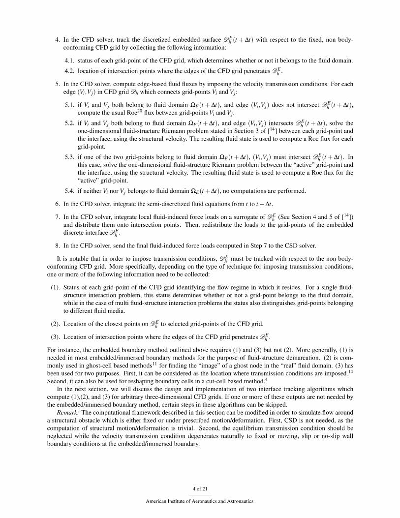
going to be used, and so adding them to the hierarchy is both unnecessary and makes the algorithm less efficient. Thekey idea behind the distribution of the bounding box hierarchy is to compute a hierarchy only over triangles near agiven fluid subdomain, creating a “scope” consisting only of triangles that are relevant to this particular subdomain.

Consider the simple two-dimensional example shown in Figure 6. The computational domain is distributed acrosssixteen subdomains, labeled in the figure, and there is a large structure (shown as an oval) near the center of the domain.A global bounding box hierarchy approach computes the hierarchy for the entire interface, on every processor. In thedistributed approach, only the component of the surface that is near a given subdomain is added to that subdomain’shierarchy. For example, Figure 6 shows Subdomain 10, as well as the component of the structure surface that isconsidered to be “near” it. This considerably reduces the size, construction time, and query time of its bounding boxhierarchy.

Figure 6. Illustration of a distributed fluid computational domain (left) and the scope of Subdomain 10 (right).

The algorithm for constructing a distributed bounding box hierarchy for either ALGORITHM 1 or ALGORITHM 2starts with constructing a global bounding box hierarchy on each processor storing all elements of DE

h . This hierarchyis then used at the first time-step to identify the candidate triangles for each grid-point, which are triangles “near”this grid-point, in the subdomain handled by each processor. These candidate triangles are gathered together on aper-subdomain basis, each forming a “scope”, or relevant component of the embedded discrete interface, for thatsubdomain. At the second time-step, the global bounding box hierarchy on each processor is replaced by the distributedone which stores only the triangles within the scope of the subdomain it handles.

Given that the embedded discrete interface moves/deforms in time, the scope of each subdomain needs to beupdated at every time-step. It is assumed that the CSD solver obeys a time-step restriction which satisfies that DE

hcrosses no more than one layer of elements in the CFD grid Dh in a given time-step. Under this assumption, the updatedsubdomain scope only needs to include (1) the current candidate triangles for each grid-point in this subdomain aswell as (2) any additional candidate triangles for each grid-point at the subdomain boundary, identified by neighboringsubdomains that share this grid-point. To obtain (2), local MPI communications across neighboring subdomains arerequired.

IV. Applications and performance assessment

The numerical algorithms presented in this paper for interface tracking were implemented in the finite volume CFDsolver AERO-F which is equipped with both the embedded boundary method14 summarized in Section II and also anALE computational framework.19, 23 In this section, proposed algorithms are demonstrated on three three-dimensional,dynamic fluid-structure interaction problems in the fields of aeronautics and underwater implosion. First, the rigidmotion of a thin airplane wing is simulated for the purpose of verification. It is considered as a practical example ofCase II in Figure 5 as the embedded discrete interface is closed but not well-resolved by the non body-conforming CFDgrid. The flow solutions obtained from the embedded boundary method using ALGORITHM 1 and 2 are compared toa reference obtained from the same CFD solver using its ALE computational framework, which has been successfullyverified and validated for many applications in the past.16, 19, 23 Next, an underwater implosion problem, for whichexperimental data is available, is used for validation. This problem features large structural deformations and strongshock waves initiated at the fluid-structure interface, which challenges both the interface tracking algorithms and theembedded boundary method. It is considered as an example of Case I in Figure 5 as the embedded discrete interfaceis both closed and well-resolved by the CFD grid. Finally, the aeroelastic simulation of a pair of extremely thin and

10 of 21


flexible wings flapping in air is considered. This is an example of Case III in Figure 5 as the embedded discreteinterface (the wings) is an open surface. It highlights the capability and robustness of interface tracking ALGORITHM2 in handling open surfaces and large structural deformations.

For the two-way coupled fluid-structure interaction simulations, AERO-F is coupled with a finite element CSDsolver using a partitioned procedure.27 The two codes communicate via run-time software channels. In particular,when the embedded boundary method in AERO-F is used, they exchange fluid and structural data efficiently via theembedded discrete interface. All computations reported in this section are performed in double-precision arithmeticon a massively parallel Linux cluster system.

In all three applications, flow solutions are compared in order to reveal the differences of interface tracking AL-GORITHM 1 and 2. This is justified by the fact that the two algorithms are treated in exactly the same way by the CFDsolver. In other words, when a simulation is repeated with a different interface tracking algorithm, any perturbation inflow solutions indicates that the output of interface tracker has changed.

Finally, it is notable that in all simulations the CFD solver, the embedded boundary method, and the interfacetracking algorithms operate on unstructured tetrahedral meshes.

IV.A. Verification for a transient subsonic flow past a heaving rigid AGARD wing

In this section, the problem of computing the unsteady airflow past a rigid wing in heaving motion is considered. Thisproblem is considered as an excellent verification problem for interface tracking algorithms as the wing representsa thin structure that is difficult to be resolved by a non body-conforming CFD grid. Moreover, the flow solutionsobtained from the embedded boundary method using the presented interface tracking algorithms can be easily verifiedagainst a reference solution obtained from an ALE simulation.

The wing considered in this problem has a root chordlength Lc = 22.0 in, a semi-span Ls = 30.0 in, a tip chordlengthLt = 14.5 in, and a quarter-chord sweep angle of 45o. Its panel aspect ratio is equal to 1.65 and its taper ratio is equalto 0.66. Its airfoil section is the NACA 65A004. A surface grid of this wing with 20,721 grid points and 41,438triangles (Figure 7–Left) is generated and will be embedded in the CFD grid.

Figure 7. Left: The embedded surface grid of the AGARD wing. Right: A non body-conforming fluid grid G1 for the simulation of the unsteady flow past arigid wing in harmonic heaving motion (cutview at z = 0).

In the coordinate system whose origin is at the leading edge of the root section of the wing, and x and y directionsare along its chord and span, respectively, the chosen computational fluid domain can be described as the rectangularbox extending from x = −500.0 in to x = 500.0 in, z = −500.0 in to z = 500.0 in, and y = 0.0 in to y = 500 in. Anon body-conforming fluid grid G1 with 609,576 tetrahedra and 105,030 grid points is generated for computing anEulerian solution for this problem using an embedded boundary method (Figure 7–Right).

Before performing flow computations, the mesh intersection results provided by interface tracking algorithms(ALGORITHM 1, 2) are assessed. Figure 8 shows the edges in G1 that are flagged as fluid-structure intersecting edgesby ALGORITHM 1 and ALGORITHM 2. It is notable that ALGORITHM 1 misses large swaths of the structure, as thefluid mesh fails to resolve the structure sufficiently. This is an example of Case II shown in Figure 5. More specifically,ALGORITHM 1 does not recognize the CFD grid edges which intersect the interface twice (at both the upper and lowersurfaces of the wing) as intersecting edges, because the two vertices of each edge share the same status. (See Step 5of ALGORITHM 1.)

11 of 21


Next, the approach for computing distributed bounding box hierarchy (scoping) presented in Section III.C is alsoinvestigated. Figure 9 shows the scope decomposition for 32 fluid computational subdomains. Compared to 41,438triangle elements in the structure surface grid, the largest subdomain scope consists of only 4,278 triangles.

Figure 8. The robustness of ALGORITHM 1 and ALGORITHM 2 is highlighted here, where we show in red a semi-transparent surface grid (Figure 7–Left), andin white the fluid mesh edges which are flagged as fluid-structure intersecting edges. Note that ALGORITHM 1 misses large swaths of the structure, as the fluidmesh fails to resolve the structure sufficiently.

Figure 9. Visualization of the scope decomposition for 32 fluid computational subdomains. Each distinct color represents the relevant component of thestructure surface grid for a different CPU, for which a bounding box hierarchy is computed.

Next, the wing is set in a harmonic heaving motion characterized by the amplitude ha = 0.05 in and the frequencyh f = 500 Hz. The free-stream conditions (Mach number, angle of attack, density, and pressure) are set to M∞ = 0.3,α∞ = 0deg, ρ∞ = 9.357255× 10−8 (lb/in4).s2, and p∞ = 14.5 psi, respectively. For comparison purpose, a body-conforming grid G2 with 4,664,720 tetrahedra and 896,167 grid points is also generated for the computation of anALE reference solution.

Symmetry boundary conditions are applied on the plane y = 0 containing the root of the wing. Non-reflectingboundary conditions are applied at the remaining boundaries of the external computational fluid domain.

Three numerical simulations are performed:

1.1. using grid G1, the embedded boundary method, and ALGORITHM 1 for interface tracking;

1.2. using grid G1, the embedded boundary method, and ALGORITHM 2 for interface tracking;

1.3. using grid G2 and the ALE computational framework.

All three simulations are initialized with a uniform flow corresponding to the free-stream conditions specifiedabove.

12 of 21


The obtained time-histories of the lift are reported in Figure 10 for the first five periods of oscillation (0 s ≤ t ≤0.01 s). The lift predicted by Simulation 1.3 can be considered as a benchmark for three reasons. First, it is com-puted on a much finer CFD grid (896,167 grid-points in G2 versus 105,030 in G1). Second, the ALE computationalframework of AERO-F has been successfully verified and validated for many applications in the past. Third, this rigidheaving problem can be easily handled by to the ALE framework as the computation of fluid mesh-motion is trivial. InFigure 10, the reader can observe that Simulation 1.1 predicts almost the same lift as the benchmark while the solutionof Simulation 1.2 is less accurate. This is not surprising given the different intersection results provided by the twointerface tracking algorithms which are shown in Figure 9.

0 0.002 0.004 0.006 0.008 0.01−300

−200

−100

0

100

200

300

400Total lift

Time (sec)

Lift

(lb.f)

ALE referenceAlgorithm 1Algorithm 2

0 0.5 1 1.5 2 2.5 3x 10−3

−300

−200

−100

0

100

200

300

400Total lift

Time (sec)Li

ft (lb

.f)

ALE referenceAlgorithm 1Algorithm 2

Figure 10. Time-history of the total lift generated by the harmonically heaving rigid wing. Comparison of the embedded boundary method equipped witheither ALGORITHM 1 or ALGORITHM 2 with the ALE framework.

Finally, timing information for Simulation 1.1 and 1.2 is reported in Table 1. They were both performed on 32 MPIprocessors. It is notable that interface tracking ALGORITHM 2 is indeed slower than ALGORITHM 1 (154 s vs. 53 s).However, given that interface tracking consumes only a small fraction (5% in Simulation 1.1 and 12% in Simulation1.2) of the total CPU time, this is acceptable. In general, the computational complexity of an implicit flow solver isO(N logN) while the computational complexity of both interface tracking algorithms is O(N logNE), where N and NEdenote the number of grid-points in the CFD grid and the number of elements in the embedded discrete interface. Inmost applications NE is much small than N given that the CFD grid is in 3D while the interface is 2D. As a result, thecost of interface tracking is significantly smaller than that of the flow solver. In this example, the ratio between NE and

N is roughly e =NE

N= 0.39. The reader will see in the next two applications when this ratio becomes smaller the cost

of interface tracking using either algorithm is actually trivial compared to the cost of flow computation.

Table 1. CPU performance on 32 processors of the simulation of the unsteady flow past a heaving rigid wing.

Simulation 1 Simulation 2Flow computations 949 s 1,019 s

Finite volume fluxes and Jacobian 170 s 198 sLinear system solution (GMRES) 629 s 641 sMesh metrics update 0 s 0 sOthers 150 s 180 s

Mesh motion update 0 s 0 sInterface tracking 53 s 154 sTotal simulation time 1,042 s 1,212 s

13 of 21


IV.B. Validation for the implosive collapse of an air-filled cylindrical shell submerged in water

In this subsection, the simulation of an underwater implosion experiment recently performed at the University of Texasat Austin is considered. This is a transient high-speed multi fluid-structure interaction problem characterized by ultra-high compressions, strong shock waves, and large structural displacements and deformations. In this problem, theembedded discrete interface is well resolved by the non body-conforming CFD grid from the beginning of simulationuntil the cylinder has fully collapsed. Hence, it can be considered as an example of Case I in Figure 5 and we expectto obtain similar solutions using ALGORITHM 1 and ALGORITHM 2.

IV.B.1. Experiment

In the experiment, an air-filled aluminum cylinder (the specimen) of length L0 = 5.0014 in, circular cross section withexternal diameter D = 1.5007 in, and thickness t = 0.0280 in is submerged in a rigid water tank. It has a maximumovalization (imperfection) ∆o = 0.083%. It is bonded at both ends to two rigid steel plugs which close the cylinder.The unbonded region of the cylinder has a length of L = 2D = 3.0014 in. (see Figure 11) The cylinder is maintainedat the center of the tank by a set of bars attached to the rigid tank. It is surrounded by 6 pressure sensors that aredistributed on the mid-plane (orthogonal to the axial direction of the cylinder) with radial distance d = 2.5± 0.25 into the center of the cylinder.

Initially, the water outside the cylinder and the air inside are both at rest (v0w = v0

a = 0 in/s). They have thesame pressure p0

w = p0a = 14.5 psi. The density of water is ρ0

w = 9.357255× 10−5 (lb/in4).s2. The density of air isρ0

a = 9.357255× 10−8 (lb/in4).s2. The water pressure is then increased slowly at a constant rate until the cylindercollapses. The final hydrostatic pressure, under which the cylinder collapses, is pco = 690.5 psi. Two photos of thecollapsed cylinder are shown in Figure 12. The time at which the cylinder starts collapsing is denoted as t = 0. Therecorded pressure time-history by Sensor 1 (see Figure 14) reveals first a gradual pressure drop of 118.0 psi before thecylinder gets into self-contact, followed by a sharp pressure rise with a peak of 1.16× 103 psi afterward. This sharppressure rise corresponds to the strong shock waves caused by the structure’s self-contact.

Figure 11. Schematic drawing of a cylindrical implodable with caps are designated by stripes (courtesy of Stelios Kyriakides).

IV.B.2. Simulation

To simulate this experiment, AERO-F is coupled with a finite element CSD solver. The geometric center of thecylinder is chosen as the origin of the Cartesian coordinate system, and its axial direction is chosen as the x-axis.In the CSD sub-problem, half of the cylinder (length-wise) is modeled. Its aluminum material is represented as anon-linear elasto-plastic medium with a Young modulus E = 1.014× 107 psi, a Poisson ratio ν = 0.3, and a densityρS = 2.599×10−4 (lb/in4).s2. The yield stress is set to 3.909×104 psi and the hardening modulus to 9.366×104 psi.

14 of 21


Figure 12. Photos of the collapsed cylinder (courtesy of Stelios Kyriakides).

The cylinder is discretized by a finite element model with 10,368 four-noded shell elements. The steel plug to whichthe cylinder is bonded is represented by 1,833 four-noded rigid shell elements. The density of these rigid elements areartificially set to ρP = 4.7363× 10−2 (lb/in4).s2 such that the total mass of these shell elements is equal to the totalmass of the volumetric steel plug used in the experiment.

A Mode 4 sinusoidal imperfection is imposed on the geometry of the cylinder to trigger its collapse. More specif-ically, the circular cross section of the cylinder is replaced by (r,θ),0≤ θ < 2π with

r = r0(1−∆cos4θ),

in which r0 = 0.73635 in is the radius of the true circular cross section measured to the mid-surface of the cylinder.The imperfection rate ∆ is set to be the same as the maximum ovalization of the specimen in the experiment, i.e.∆ = ∆o = 0.083%.

In the CFD sub-problem, air inside the cylinder is modeled as perfect gas with a specific heat ratio γa = 1.4.Because of the ultrahigh compressions involved in this problem, water is modeled as stiffened gas whose equation ofstate can be written as

(γ−1)ρe = p+ γ p0,

where e denotes the internal energy per unit mass, and γ and p0 are two constants that are set here to γw = 4.4and p0 = 8.7× 107 psi. The fluid computational domain is a rectangular box: Ω = (x,y,z) ∈ R3 : 0 in ≤ x ≤12 in, −10 in≤ y≤ 10 in, −10 in≤ z≤ 10 in. An unstructured non body-conforming CFD grid G1 with 1,689,089grid-points and 10,064,277 tetrahedral elements is generated to discretize Ω (Figure 13). An embedded surface grid(GE ) is generated using the same node set as in the structure grid and triangle elements obtained by dividing eachquadrangle element in the structure grid into two triangles. It contains 12,275 grid-points and 24,404 elements.

Symmetry boundary conditions are applied to both the fluid and structure models at x = 0. Non-reflectingboundary conditions are applied to the remaining boundaries of the fluid domain. Sliding boundary conditions areapplied to the plug as well as the bonded region of the cylinder such that only displacement along x direction isallowed. At t = 0, the initial state of air inside the cylinder is set to ρ0

a , v0a, and p0

a. The initial state of water is set toρ0

w, v0w, and p∗a = pco− 10 psi. In the first 1.5× 10−4 sec of the simulation, the water pressure is increased statically

and linearly to pco, whereas the air pressure inside the cylinder remains at p0a. At t = 1.5×10−4 sec, when the collapse

pressure pco is reached, the compressible flow solver is activated.Two simulations are performed using the embedded boundary method. The embedded discrete interface is tracked

by ALGORITHM 1 in one simulation (denoted by Simulation 2.1) and ALGORITHM 2 in the other (denoted by Sim-ulation 2.2). Both simulations are carried out on 261 MPI processors (260 for the CFD solver, 1 for the CSD solver)until T = 1.5×10−3 sec. The water pressure histories at the sensor locations are recorded.

The predicted pressure histories at Sensor 1 and 2 are shown in Figure 14 together with the experimental data.As expected, the solutions given by the two simulations are very close. More importantly, the main features in theexperimental data, particularly the amplitude of the highest peak and the width of the pressure jump, are accuratelycaptured for both sensors in both simulations.

15 of 21


Figure 13. The fluid computational domain with the embedded surface (left) and a cut-view of CFD grid G1 at z = 0.

0 0.2 0.4 0.6 0.8 1 1.2 1.4 1.6x 10−3

500

600

700

800

900

1000

1100

1200Sensor 1

Time (sec)

Pres

sure

(psi

)

ExperimentAlgorithm 1Algorithm 2

0 0.2 0.4 0.6 0.8 1 1.2 1.4 1.6x 10−3

500

600

700

800

900

1000

1100

1200Sensor 2

Time (sec)

Pres

sure

(psi

)

ExperimentAlgorithm 1Algorithm 2

Figure 14. Comparison of the predicted pressure time-histories obtained from Simulation 2.1 (using ALGORITHM 1) and 2.2 (using ALGORITHM 2) with theexperimental data. Left: Sensor #1; Right: Sensor #2.

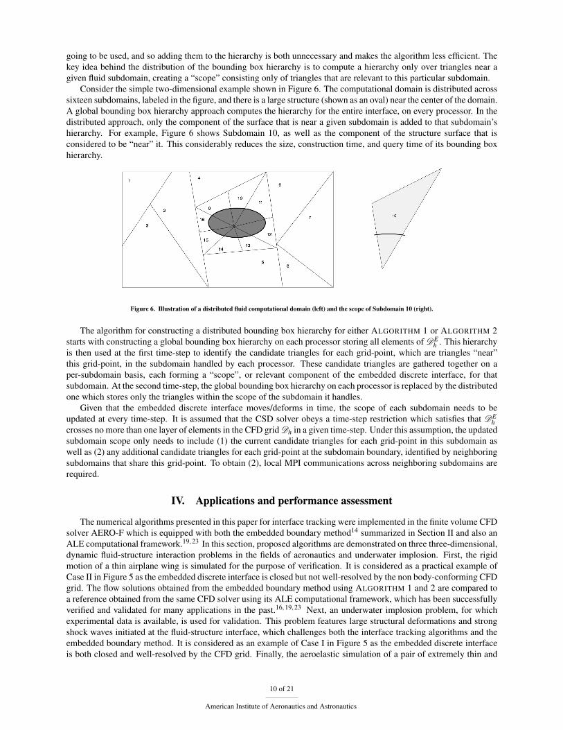
The predicted deformation of the structure model at final time T = 1.5× 10−3 sec is shown in Figure 15. Pre-dictions by Simulation 2.1 and Simulation 2.2 are visually the same so only the one obtained from Simulation 2.1 isshown. The reader can observe that it is similar to the experimental result shown in Figure 12.

In this problem, the ratio between the number of elements in the embedded discrete interface (NE ) and the number

of grid-points in the CFD grid (N), is given by e =NE

N= 0.014. The CPU time consumed for interface tracking is

566 s in Simulation 2.1 and 1,355 s in Simulation 2.2, which account for only 1.9% and 4.1% of the total simulationtime.

IV.C. Application to the fluid-structure interaction problem with ultra-thin flapping wings

Here the aeroelastic simulation of a pair of flapping wings is considered. The surface of these wings are made ofpolyester film. With a thickness of only 0.16 mm, they are extremely flexible. This brings significant difficulties tothe aeroelastic simulation as the structure model is very sensitive to numerical error. The surface of these wings isrepresented by one layer of shell elements in both the CSD model and the embedded discrete interface. As a result, theembedded discrete interface is no longer a closed surface and thus can be handled by interface tracking ALGORITHM2 but not ALGORITHM 1. This is a practical example of Case III in Figure 5.

The dimension of the structure model and the CSD grid are shown in Figure 16. Connected at the centerline x = 0,the two triangular wings share the same dimension and materials. The CSD grid is symmetric with respect to centerlinex = 0. The polyester film material for the surface of the wings including the reinforced region (shown in green in

16 of 21


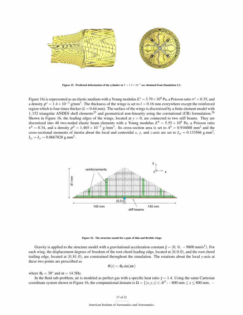
Figure 15. Predicted deformation of the cylinder at T = 1.5×10−3 sec obtained from Simulation 2.1.

Figure 16) is represented as an elastic medium with a Young modulus Es = 3.79×109 Pa, a Poisson ratio νs = 0.35, anda density ρs = 1.4×10−3 g/mm3. The thickness of the wings is set to l = 0.16 mm everywhere except the reinforcedregion which is four times thicker (L= 0.64 mm). The surface of the wings is discretized by a finite element model with1,152 triangular ANDES shell elements25 and geometrical non-linearity using the corotational (CR) formulation.26

Shown in Figure 16, the leading edges of the wings, located at y = 0, are connected to two stiff beams. They arediscretized into 48 two-noded elastic beam elements with a Young modulus Eb = 5.55× 109 Pa, a Poisson ratioνb = 0.34, and a density ρb = 1.465× 10−3 g /mm3. Its cross-section area is set to Ab = 0.916088 mm2 and thecross-sectional moments of inertia about the local and centroidal x, y, and z-axis are set to Ixx = 0.133566 g.mm2,Iyy = Izz = 0.0667828 g.mm2.

x

y

z

(0,0,0)

stiff beams

reinforcements

140 mm

81 m

m

140 mm

Figure 16. The structure model for a pair of thin and flexible wings

Gravity is applied to the structure model with a gravitational acceleration constant~g = (0, 0, −9800 mm/s2). Foreach wing, the displacement degrees of freedom of the root chord leading edge, located at (0,0,0), and the root chordtrailing edge, located at (0,81,0), are constrained throughout the simulation. The rotations about the local y-axis atthese two points are prescribed as

θ(t) = θ0 sin(ωt)

where θ0 = 38o and ω = 14.5Hz.In the fluid sub-problem, air is modeled as perfect gas with a specific heat ratio γ = 1.4. Using the same Cartesian

coordinate system shown in Figure 16, the computational domain is Ω = (x,y,z)∈R3 :−800 mm≤ x≤ 800 mm, −

17 of 21


400 mm ≤ y ≤ 400 mm, −400 mm ≤ z ≤ 400mm (Figure 17). A non body-conforming CFD grid with 2,086,997grid points and 12,462,983 tetrahedral elements is generated (Figure 17, 18). As mentioned, the embedded surface isan open surface. It is generated using the same set of triangular elements in the CSD grid for the surface of the wings.It contains 650 grid-points and 1,152 elements.

Figure 17. The computational fluid domain for the aeroelastic simulation of flapping wings.

Figure 18. The non body-conforming CFD grid for the aeroelastic simulation of flapping wings. Left: cutview at y = 5 mm. Right: cutview at z = 0 mm.

Non-reflecting boundary conditions are applied to all the boundaries of Ω. At time t = 0, the fluid is initializedusing a uniform state of density ρ = 1.3×106 g/mm3, velocity v = 0 mm/s, and pressure p = 105 g/(mm.s2) = 105 Pa.

Interface tracking ALGORITHM 2 is first verified by visually inspecting the intersecting edges it identified. Fig-ure 19 displays the identified intersecting edges near a wing-tip represented by gray bars, and the embedded discreteinterface it penetrates in red. Status of the end-points of intersecting edges are also displayed in color. The reader canobserve that they share the same color (green), which implies that they are identified to reside in the same flow medium(air). To summarize, Figure 19 shows that ALGORITHM 2 successfully determined the status of CFD grid-points andat the same time correctly identified intersecting edges.

An aeroelastic simulation (denoted by Simulation 3.1) using the embedded boundary method and ALGORITHM2 for tracking the embedded discrete interface is performed on 261 (260 for the CFD solver, 1 for the CSD solver)MPI processors. The termination time is set to T = 0.3 sec, which corresponds to roughly four cycles of flapping. Thetime-history of displacement along z-axis is reported in Figure 20 for the tip of one wing, located initially at (140,0,0).The maximum amplitude is about 100 mm,or 71% of the length of semi-span. Color plots of the fluid pressure fieldtogether with the structural deformation at six time instances are shown in Figure 21. The large deformations and highfrequency local vibrations on the structure model are clearly evident.

18 of 21


Figure 19. Identified intersecting edges and status on their end-points near the tip of a flapping wing.

In this simulation, the cost of interface tracking is negligible, as it consumes only 0.5% of the total simulation time(108 seconds vs. 5.9 hours). This is the consequence of a very small ratio between the number of elements in the

embedded discrete interface (NE ) and the number of grid-points in the CFD grid (N). More specifically, e =NE

N=

5.5×10−4.

0 0.05 0.1 0.15 0.2 0.25 0.3

−100

−50

0

50

100

Tip displacement along z−axis

Time (sec)

Dis

plac

emen

t (m

m)

Simulation 3.1

Figure 20. Time history of the tip displacement in z-axis for one of the wings.

V. Conclusions

Focusing on the context of embedded/immersed boundary methods for Computational Fluid Dynamics (CFD),this paper contributes two robust and efficient algorithms, referred to as ALGORITHM 1 and 2, for tracking embed-ded/immersed fluid-structure interfaces with respect to three-dimensional, arbitrary CFD grids. Both algorithms takeadvantage of the bounding box hierarchy to optimize the efficiency. For distributed flow computations, an algorithmfor constructing distributed bounding box hierarchies is also presented. These algorithms are applied to an embeddedboundary method and their performances are assessed in three dynamic fluid-structure interaction problems. More

19 of 21


Figure 21. Snapshots of the fluid pressure field (cutview at y = 20 mm) and the structural deformation at six time instances.

specifically, these algorithms are first verified for a transient subsonic flow past a heaving rigid AGARD wing, forwhich reference results are obtained from a simulation using the ALE computational framework on a refined body-conforming grid. The results obtained using ALGORITHM 2 matches the reference excellently whereas the onesobtained using ALGORITHM 1 are less accurate. This application reveals the accuracy advantage of ALGORITHM 2in handling thin structures embedded in coarse CFD grids. Next, an underwater implosion problem is used to validatethe embedded boundary method equipped with algorithms proposed in this paper. It also verifies that when the em-bedded/immersed interface is closed and well-refined by the CFD grid, ALGORITHM 1 and ALGORITHM 2 providesimilar, and accurate results. Finally, the capability and robustness of ALGORITHM 2 in tracking open surfaces arehighlighted in an application to the fluid-structure interaction problem with ultra-thin flapping wings. In terms ofefficiency, in all three applications, the computational cost of interface tracking using either algorithm is very smallcompared to the total simulation cost (from 0.5% to 12%). ALGORITHM 2 is 2 to 3 times slower than ALGORITHM1, which is understandable as it requires more expensive collision detection tests.

Acknowledgments

The authors acknowledge partial support by the Office of Naval Research under Grant N00014-06-1-0505 andGrant N00014-09-C-015, partial support by the Army Research Laboratory through the Army High PerformanceComputing Research Center under Cooperative Agreement W911NF-07-2-0027, and partial support by The BoeingCompany under Contract Sponsor Ref 45047. The content of this publication does not necessarily reflect the positionor policy of any of these supporters, and no official endorsement should be inferred. The authors also thank Dr. MichelLesoinne for his contribution to the design of the projection-based interface tracking algorithm.

References1Peskin CS. Flow patterns around heart valves: a numerical method. Journal of Computational Physics 1972; 10:252-271.2Johansen H, Colella P. A Cartesian grid embedded boundary method for Poisson’s equation on irregular domains. Journal of Computational

Physics 1998; 147:60–85.3Udaykumar H, Mittal R, Shyy W. Computation of solid-liquid phase fronts in the sharp interface limit on fixed grids. it Journal of Compu-

tational Physics 1999; 153:535–574.4Udaykumar H, Mittal R, Rampunggoon P, Khanna A. A sharp interface Cartesian grid method for simulating flows with complex moving

boundaries. Journal of Computational Physics 2001; 174:345–380.5Gilmanov A, Sotiropoulos F. A hybrid Cartesian/immersed boundary method for simulating flows with 3D, geometrically complex, moving

bodies. Journal of Computational Physics 2005; 207:457–492.

20 of 21


6Guendelman E, Selle A, Losasso F, Fedkiw R. Coupling water and smoke to thin deformable and rigid shells. SIGGRAPH 2005, ACM TOG24 2005; 973-981.

7Glowinski R, Pan TW, Kearsley AJ, Periaux J. Numerical simulation and optimal shape for viscous flow by a fictitious domain method.International Journal for Numerical Methods in Fluids 2005; 20:695–711.

8Deiterding R, Radovitzky R, Mauch S, Noels L, Commings J, Meiron D. A virtual test facility for the efficient simulation of solid materialresponse under strong shock and detonation wave loading. Engineering with Computers 2006; 22:325–347.

9Kreiss HO, Petersson A. A second-order accurate embedded boundary method for the wave equation with Dirichlet data. SIAM Journal ofScientific Computation 2006; 27:1141–1167.

10Cirak F, Deiterding R, Mauch S. Large-scale fluid–structure interaction simulation of viscoplastic and fracturing thin-shells subjected toshocks and detonations. Computers and Structures 2007; 85:1049–1065.

11Mittal R, Dong H, Bozkurttas M, Najjar F.M, Vargas A, von Loebbecke A. A versatile sharp interface immersed boundary method forincompressible flows with complex boundaries. Journal of Computational Physics 2008; 227:4825–4852.

12Robinson-Mosher A, Shinar T, Gretarsson J, Su J, Fedkiw R. Two-way coupling of fluids to rigid and deformable solids and shells. SIG-GRAPH 2008, ACM TOG 27 2008; 46.1–46.9.

13Gretarsson J, Kwatra N, Fedkiw R. Numerically Stable Fluid-Structure Interactions Between Compressible Flow and Solid Structures.Journal of Computational Physics 2011; 230:3062–3084.

14Wang K, Rallu A, Gerbeau J-F, Farhat C. Algorithms for interface treatment and load computation in embedded boundary methods for fluidand fluid-structure interaction problems. International Journal for Numerical Methods in Fluids, (in press)

15Mittal R, Iaccarino G. Immersed boundary methods. Annual Review of Fluid Mechanics 2005; 37:239–261.16Farhat C, Rallu A, Wang K, Belytschko T. Robust and provably second-order explicit-explicit and implicit-explicit staggered time-integrators

for highly nonlinear fluid-structure interaction problems. International Journal for Numerical Methods in Engineering, International Journal forNumerical Methods in Engineering 2010; 84:73–107.

17Farhat C, Lesoinne M, Maman N. Mixed explicit/implicit time integration of coupled aeroelastic problems: three-field formulation, geometricconservation and distributed solution. International Journal for Numerical Methods in Fluids 1995; 21:807–835.

18Farhat C, Geuzaine P, Grandmont C. The discrete geometric conservation law and the nonlinear stability of ALE schemes for the solution offlow problems on moving grids. Journal of Computational Physics 2001; 174: 669–694.

19Farhat C, Geuzaine P, Brown G. Application of a three-field nonlinear fluidstructure formulation to the prediction of the aeroelastic parame-ters of an F-16 fighter. Computers & Fluids 2003; 32:3–29.

20Roe PL. Approximate Riemann solvers, parameters vectors and difference schemes. Journal of Computational Physics 1981; 43:357–371.21Agarwal P.K., de Berg M, Gudmundsson J, Hammar M, Haverkort H.J. Box-trees and R-trees with near-optimal query time. Discr. Comput.

Geom. 28 , 291312 (2002)22Bridson R, Fedkiw R, and Anderson J. Robust treatment of collisions, contact and friction for cloth animation. ACM Trans. Graph. 21 (2002),

no. 3, 594-60323Geuzaine P, Brown G, Harris C, Farhat C. Aeroelastic dynamic analysis of a full F-16 configuration for various flight conditions. AIAA

Journal 2003; 41:363–371.24Farhat C, Lesoinne M, LeTallec P. Load and motion transfer algorithms for fluid/structure interaction problems with non-matching discrete

interfaces: momentum and energy conservation, optimal discretization and application to aeroelasticity. Computer Methods in Applied Mechanicsand Engineering 1998; 157:95114.

25Felippa C, and Militello C. Membrane triangles with corner drilling freedoms – II. The ANDES element. Finite Elements in Analysis andDesign 1992; 12:189-201.

26Felippa C, and Haugen B. A unified formulation of small-strain corotational finite elements: I. Theory. Computer Methods in AppliedMechanics and Engineering 2005; 194:2285–2335.

27Piperno S, Farhat C, Larrouturou B. Partitioned procedures for the transient solution of coupled aeroelastic problems Part I: Model problem,theory and two-dimensional application. Computer Methods in Applied Mechanics and Engineering 1995; 124:79–112

28Lohner R, Applied computational fluid dynamics techniques: an introduction based on finite element methods (second ed.), John Wiley &Sons (2008) ISBN 978-0-470-51907-3.

21 of 21


numerical algorithms for tracking dynamic fluid-structure ... filebody-conforming computational...

Documents