ORIGINAL ARTICLE

Numerical analysis of different heating systems for warm sheetmetal forming

J. M. P. Martins1 & J. L. Alves2 & D. M. Neto1 & M. C. Oliveira1 & L. F. Menezes1

Received: 17 April 2015 /Accepted: 19 July 2015 /Published online: 2 August 2015# Springer-Verlag London 2015

Abstract The main goal of this study is to present an analysisof different heating methods frequently used in laboratoryscale and in the industrial practice to heat blanks at warmtemperatures. In this context, the blank can be heated insidethe forming tools (internal method) or using a heating system(external method). In order to perform this analysis, a finiteelement model is firstly validated with the simulation of thedirect resistance system used in a Gleeble testing machine.The predicted temperature was compared with the tempera-ture distribution recorded experimentally and a good agree-ment was found. Afterwards, a finite element model is used topredict the temperature distribution in the blank during theheating process, when using different heating methods. Theanalysis also includes the evaluation of a cooling phase asso-ciated to the transport phase for the external heating methods.The results of this analysis show that neglecting the heatingphase and a transport phase could lead to inaccuracies in thesimulation of the forming phase.

Keywords Heatingmethods . Light-weight alloys .Warmforming conditions . Finite element method

1 Introduction

The automotive industry has made significant efforts in recentyears to reduce the fuel consumption in passenger cars andconsequently reduce the carbon dioxide (CO2) emissions ratesto fulfill the new environmental demands [1]. The adoption oflight-weight materials, such as aluminium [2] and magnesiumalloys [3], allows the weight reduction in body-in-white.Therefore, the actual trend in this industry consists in replac-ing traditional mild steels by light-weight materials. Althoughthese alloys present high-strength-to-weight ratio and excel-lent corrosion resistance, the formability of these alloys atroom temperature is considerably low when compared withlow carbon steels, which limits its widespread application [4].However, the formability can be significantly improved bywarm forming, since the increase of temperature leads to adecrease in the material flow stress and improves the ductility[5].

Typically, the warm sheet metal forming process of light-weight alloys is performed in the temperature range of 200 to350 °C, below the recrystallization temperature to avoid mi-crostructural changes. The behaviour of two Al–Mg–Si alloysduring drawing was investigated by Ghosh et al. [6] at roomand warm temperatures, concluding that the force–displace-ment evolution is strongly influenced by the blank tempera-ture. Moreover, the formability (limiting drawing ratio) andductility of these alloys is enhanced by the warm tempera-tures, as illustrated byAbedrabbo et al. [7]. Another advantageof warm forming processes is the decrease of the springbackeffects, resulting from the change of the stress state in theformed sheet [8]. The experimental and numerical study

* J. M. P. Martinsjoao.pmartins@dem.uc.pt

J. L. Alvesjlalves@dem.uminho.pt

D. M. Netodiogo.neto@dem.uc.pt

M. C. Oliveiramarta.oliveira@dem.uc.pt

L. F. Menezesluis.menezes@dem.uc.pt

1 CEMUC, Department of Mechanical Engineering, University ofCoimbra, Polo II, Rua Luís Reis Santos, Pinhal de Marrocos,3030-788 Coimbra, Portugal

2 MEMS, Microelectromechanical Systems Research Unit, Universityof Minho, Campus de Azurém, 4800-058 Guimarães, Portugal

Int J Adv Manuf Technol (2016) 83:897–909DOI 10.1007/s00170-015-7618-9

performed byGrèze et al. [9] shows that the stress gradient in acylindrical cup wall decreases with the temperature, reducingthe springback observed in the split-ring test. They concludethat the distribution of the hoop stress in the cup wall is themain factor influencing the springback mechanism in warmforming condition. In addition to the above-mentioned bene-fits, the stretcher lines arising in the AA5xxx series (Al–Mgalloys) due to the Portevin–Le Chatelier (PLC) effect vanish atwarm temperatures, as highlighted in the experimental studyperformed by Coër et al. [10].

In comparison with the conventional sheet metal formingprocesses, the warm forming requires an additional stage toincrease the temperature of the blank before the forming op-eration. Two distinct strategies can be adopted for the heatingprocess: (1) generate a uniform (warm) temperature in thewhole blank or (2) apply a gradient of temperatures in theblank, i.e., increase the temperature in some regions andcooling others [11]. An example of the former strategy hasbeen recently proposed by Hung and Merklein [12] using alaser system for local heat treatment of the blank in order toenhance its formability. However, since this heating procedurerequires a deep knowledge of the interaction between mechan-ical and thermal effects on formability, the concept commonlyused in industry is still the uniform heating of the blank [13].Concerning this simple strategy, the heating of the blank canbe carried out using two different heating methods: (1) exter-nal heating in furnaces, induction systems or direct resistancesystems and (2) internal heating by conduction through heatedtools on the press. The systems used in the external heatingcan be classified by direct and indirect according to the heattransfer mechanism [14]. The conventional furnaces are theheating systems commonly employed by the industry due toits high production flexibility and availability. On the otherhand, on a laboratory or R&D scale the temperature of theblank is usually raised by internal heating by means of con-duction with heated tools [15]. Nevertheless, this last proce-dure involves complex tool systems with high costs (electricalresistance heaters inserted at different locations in the tool),and can increase substantially the process lead time, eliminat-ing the high productivity rates characteristic of the metalforming processes.

The temperature distribution in the blank immediately be-fore the forming operation is a key point for the success of thewarm sheet metal forming processes [6]. However, thisheating stage is typically overlooked in the numerical model-ling of the process, as well as the cooling of the blank thatoccurs during its transport to the press, in case of externalheating [16]. In fact, the temperature of the blank is commonlyassumed uniform at the beginning of the forming stage in thefinite element analysis. Therefore, this study intends to im-prove the finite element modelling of the warm sheet metalforming processes by taking into account both the initialheating stage and the subsequent transfer period (air cooling),

when considering external heating systems. In this context,the algorithm for the thermal analysis was implemented inthe finite element code DD3IMP [17], which has been specif-ically developed to simulate sheet metal forming processes. Itskey feature is the use of a fully implicit algorithm of Newton–Raphson type to solve, within a single iterative loop, the non-linearities related with both the mechanical behaviour and thefrictional contact [18].

The comparison between the different heating methods fre-quently used in warm forming processes is presented in thiswork. The transient thermal problem (blank heating) isanalysed with the finite element method considering both con-duction and convection mechanisms. The developed finiteelement code and the numerical model are validated with ex-perimental results from a tensile specimen heated by Joule’seffect (Gleeble system). Moreover, the heating stage for thewarm sheet metal forming of an automotive B-pillar is pre-sented in detail, comparing different heating methods throughfinite element simulation.

2 Heating methods

This section presents a review of different heating methodstypically adopted in warm sheet metal-forming processes,both in laboratory scale as well as in industrial practice.

2.1 Furnaces

The heating process through furnace is the conventional meth-od used in industry, where the heat can be generated either byfossil fuels or electricity [19]. The procedure consists in load-ing the blank into the furnace in order to raise its temperatureup to the warm forming temperature. Since the blank is heatedmainly by convective flow from the heat source, the furnacesare slow heating systems. Indeed, the final temperature of theblank is dictated by the exposure time and the temperature ofthe furnace. Since the ratio between exposed surface and vol-ume is very high in metallic sheets, the temperature gradientsbetween the core and the sheet surface are negligible.

The heating system adopted by Takuda et al. [20] in thewarm deep drawing of an aluminium alloy 5182-O is thefurnace. The forming tools (die and blank-holder) are heatedtogether with the blank sheet until 250 °C and then assembledinto the press. This experimental procedure allows to avoidheat losses to the tools during the forming stage. The metal-lography of the austenitic stainless steel 304 after warm deepdrawing was studied by Lade et al. [21]. They also heated theblank and the die using a furnace to carry out warm formingtests at temperatures on the range between 150 and 300 °C.The mechanical characterisation for warm forming tempera-ture of the magnesiumAZ31 alloy sheet for was performed byKoh et al. [22] using a numerical inverse approach. The deep

898 Int J Adv Manuf Technol (2016) 83:897–909

drawing of a cylindrical cup was the example selected, whereboth the blank and the forming tools, except the punch, wereheated in an external furnace until reaching 280 °C. Due to theheat loss to the environment during the moving and setting,the blank temperature decreases about 15 °C in 5 s. The me-chanical behaviour of three commercial magnesiumsheet alloys was studied by Krajewski [23] at warm tempera-tures. The blanks were heated in a furnace on the range oftemperatures between 200 and 400 °C. Its temperature wasmeasured immediately before the forming process and wasabout 50 °C cooler than the temperature at the furnace exit,highlighting the heat losses to the environment during themovement of the blank to the press. In order to optimize thewarm forming process in terms of production robustness andcosts, Harrison et al. [16] present a non-isothermal method.Only the blank (5182-O aluminium alloy) was heated inside afurnace using an exposure time of 180 s to reach the warmforming temperature. After the heating process, the blank wasmoved to the press using a robot, consuming about 15 s in thisoperation. The heat losses for the tools were not avoided, infact, they were intentional in order to obtain a non-isothermalcondition after the forming stage.

2.2 Induction heating

The application of an alternating current in an induction coilgenerates a magnetic field, which induces eddy currents inelectrically conductive objects located in the vicinity of thecoil (Faraday’s law). Consequently, this produces heat as aresult of the Joule’s effect [13]. The frequency and the inten-sity of the induced current, as well as the material properties(specific heat, magnetic permeability and electrical resistivity)define the heating rate of the body. Since the aluminium alloyspresent low electrical resistivity when compared with steelalloys, they require a longer heating stage to attain the sametemperature [24]. Since the current density decreases expo-nentially towards the body centre, leading to a non-uniformcurrent distribution within the body, the so called skin-effect isdirectly related with this heating system. This effect can berelieved by decreasing the current frequency. The thermo-mechanical properties of the aluminium alloy 7000-T4 wereevaluated by Codrington et al. [25] at 260 and 480 °C using anew induction heating apparatus developed by the authors.Takuda et al. [26] studied the flow stress evolution of a com-mercial magnesium alloy AZ31 at warm temperaturesadopting an induction system to achieve the required temper-atures. The mechanical properties of the magnesium alloyAZ31B at different temperatures and strain rates were inves-tigated by Pellegrini et al. [27] using an induction heatingsystem. The temperature range between 200 and 300 °C wasselected and a constant heating rate of 3 °C/s was applied. Inorder to assure a uniform temperature field, the specimen wasmaintained at this temperature during 120 s.

2.3 Direct resistance heating

In case of the direct resistance heating, the blank is connected inseries with a power source. The material resistance to the pas-sage of current produces heat by Joule’s effect. The heatingrates are directly related with the current intensity and the ma-terial properties. In fact, materials with higher electric resistivitypresent larger resistance to the current flow, leading to a moreefficient heating procedure. The main limitation of this heatingsystem is related with its range of application, which is restrict-ed to sheets with constant cross-section. The variation of thecross-sectional area in the current direction yields a non-uniform temperature along the blank, i.e., the temperature be-comes higher for small cross-sectional areas and lower for largecross-sectional areas, respectively [28]. Mori et al. [29] present-ed a study concerning warm and hot stamping process usingresistance heating. The experimental work was developed in anew apparatus which was developed by the authors, consistingin a press coupled with a direct resistance heating system. Theyachieved a temperature of 850 °C in 1.5 s. Furthermore, theysynchronised the press with the heating system to minimizingthe heat loses, allowing to accomplish the forming operation0.2 s after the end of the heating phase. Since the mechanicalcontact between the sheet and the electrode is not perfect andhomogeneous, the generated temperature field is non-uniformin the contact area. This heating system provides high heatingrates using a simple apparatus, being adequate for characterisa-tion of materials at elevated temperatures. Das et al. [30] inves-tigated the mechanical properties of a magnesium alloyAZ31 at warm temperature, using a Gleeble 3800 thermo-mechanical simulator. The tensile specimens were heated bydirect resistance to 200 °C and were held at this temperatureduring 1 min. The same thermo-mechanical simulator was usedby Coër et al. [31] to study the influence of temperature on themechanical behaviour of an aluminium alloy AA5754-O dur-ing plastic deformation. Ghosh et al. [6] presented a descriptionof the behaviour of two Al–Mg-Si alloys during drawing andpost drawing. The equipment used to perform the tensile testswas also a Gleeble testing machine.

2.4 Heating by conduction with heated forming tools

The heating of a blank with pre-heated tools is typically usedin the warm deep drawing at laboratory scale. In this case,both the die and the blank-holder are pre-heated to the warmforming temperature [4], while the blank is heated by contactconduction with the tools when it is clamped between theblank-holder and die. The tools are commonly heated by elec-tric heating elements and the location of these elements de-pends on the set-up used. The main advantage of this processis to avoid the loss of heat during the transport stage, since theblank is already in the position to be formed [32]. However, alarge amount of material volume (tools) has to be heated and

Int J Adv Manuf Technol (2016) 83:897–909 899

the time required to achieve a uniform temperature of theblank might be high. This heating method is commonly usedfor attaining non-isothermal distributions on the blank [33].Lee et al. [34] have studied the formability of an AZ31 mag-nesium sheet by experimental and numerical analysis. Thesquare cup drawing is performed at various temperaturesusing a tooling system heated by cartridge heaters. Laurentet al. [8] focused on the warm deep drawing of an AA5754-O aluminium alloy, presenting a new experimental set-up de-signed to perform cylindrical cup forming tests. In this case,the blank was heated by thermal contact with the die and theblank-holder during 500 s to guarantee a uniform temperaturein the blank.

3 Finite element method

3.1 Heat transfer analysis

The differential equation of heat conduction, often called heatequation, can be derived from the law of conservation of en-ergy (first law of thermodynamic) applied to a continuousmedium with arbitrary volume (V∈ℝ3) bounded by a closedsurface S. The solution of the heat equation gives the temper-ature distribution of the arbitrary volume with respect to timeand can be expressed as follows:

ρc∂T∂t

þ div qkð Þ ¼q�; ð1Þ

where ρ and c represent the specific mass and the specific heatof the continuous medium, respectively. The vector qk repre-sents the conduction heat flux and q

�is the energy rate gener-

ation per unit of volume. The heat conduction flux is definedby the Fourier law of conduction, as follows:

qk ¼ −kgrad Tð Þ; ð2Þwhere k is the conductivity tensor. Combining Eq. (1) and (2),the relation governing the heat conduction can be written as:

ρc∂T∂t

¼ div kgrad Tð Þ½ �þ q�: ð3Þ

The classical boundary heat exchanges conditions com-prise the heat transfer modes of convection and radiation. Tomodel the convection boundary condition it is necessary toknow the convection coefficient hc and the exterior tempera-ture T∞ in order to define the convection heat flux as follows:

qconv ¼ hc T−T∞ð Þ: ð4Þ

The radiation boundary condition term is defined alsobased on a heat flux:

qrad ¼ hr T−T surð Þ; ð5Þ

in which the hr is defined by:

hr ¼ εσ T2 þ T2sur

� �T þ T surð Þ; ð6Þ

where Tsur is the surrounding temperature, ε is the emissivityof the surface and σ is the Stefan–Boltzmann constant.

3.2 Numerical implementation

3.2.1 Finite element discretization

Applying the principle of virtual temperatures to the strongform [35], the general heat equation can be written in the weakform as follows:

∫V δTρcT˙dV þ ∫VgradðδTÞ ⋅ k⋅grad Tð Þ½ �dV þ ∫SδThconvTdS þ ∫SδThrTdS ¼

∫V δT q�dVþ∫SδThconvT∞dS þ ∫SδThrT surdS: ð7Þ

The weak form is obtained by multiplying the governingEq. (3) and the convection and radiation boundary conditions(Eqs. (4) and (5)) by an arbitrary virtual temperature distribu-tion δT and integrating over the domains on which they hold.According with this principle, T is the solution of the temper-ature distribution in the body if and only if Eq. (7) holds forany arbitrary virtual temperature distribution δT that is contin-uous and satisfies the boundary conditions.

The finite element method involves the division of the vol-umeVunder consideration into finite elements. The temperatureinside a finite element is interpolated using the shape functionsand the temperatures at nodes, which can be approximated by:

T x; tð Þ¼N xð ÞΤ tð Þ for V ∀t∈�0; t f �;

T x; tð Þ¼Ns xð ÞΤ tð Þ for S ∀t∈� 0; t fð �;

ð8Þ

where tf denotes the final instant of the process. Ν(x) and Νs(x)are matrices containing the shape functions associated with thevolume and the surface of the body, respectively. Thus, thediscretized finite element equations for heat transfer problemscan be written as follows:

C T� þ Kcond þKconv=rad

� �T¼Qþ f ð9Þ

where C is the thermal capacity matrix and Kcond and Kconv/rad

are the conductivity and the convection/radiation stiffness ma-trices, respectively. Q and f are the vectors of heat generationand heat fluxes on the surface, respectively. These matrices andvectors can be expressed as:

C ¼ ∫VNTρcNdV ð10Þ

900 Int J Adv Manuf Technol (2016) 83:897–909

Kcond ¼ ∫VMTkMdV ð11Þ

Kconv=rad ¼ ∫SNTs hconvNsdS þ ∫SNT

s hrNsdS ð12ÞQ ¼ ∫VNT q

�dV ð13Þ

f ¼ ∫SNTs hconvT∞dS þ ∫SNT

s hrTrdS ð14Þ

where Μ=grad(N). The vector of internal heat generation(Eq. (13)) comprises the heat generated in the volume V bydifferent sources such as electrical resistance heating or induc-tion [36].

3.2.2 Time integration method

In transient heat conduction analysis, Eq. (9) must be integratedover the time. Different time integration methods based on oneor more time steps are available [37]. In this work, the methodadopted is a one-time step method, often named the generalizedtrapezoidal method [38]. This time integration method can bededuced from the Taylor’s expansion series, by neglecting thesecond and higher-orders terms and introducing a timeweightingfactor α varying between 0 and 1. Thus, the temperature field atinstant t+Δt is obtained using the following equation:

TtþΔt ¼ Tt þ αT�

tþΔt þ 1−αð ÞT� th i

Δt: ð15Þ

Applying the definition of the trapezoidal method intoEq. (9), the following expression is obtained:

1

ΔtCþα Kcond þKconv=rad

� �� �TtþΔt−

1

ΔtC− 1−αð Þ Kcond þ Kconv=rad

� �� �Tt¼

1−αð ÞQt þ αQtþΔtþ 1−αð Þf t þ α f tþΔt:

ð16Þ

Depending on the value selected for α, the generalizedtrapezoidal method takes the form of well-known time inte-gration methods such as, Euler forward method (α=0), CrankNickolson method α ¼ 1

2

� �, Galerkin method α ¼ 2

3

� �and

Euler backward method (α=1) [39].Only the Euler backward is known to be unconditionally

stable for non-linear thermal problems [40], i.e. starting from athermal equilibrium state at time t, it reaches a thermal equi-librium state at time t+Δt. Therefore, assuming (α=1),Eq. (16) takes the following form:

1

ΔtCþ Kcond þKconv=rad

� �� �TtþΔt−

1

ΔtC

� �Tt¼QtþΔt þ f tþΔt;

ð17Þ

which is typically solved with the Newton–Raphson iter-ative method, guaranteeing the equilibrium in all

increments. The non-linear system presented in Eq. (17)can be rewritten in a simplified way, as follows:

KGTtþΔt−PtþΔt¼RtþΔt; ð18Þ

where KG and Pt+Δt assume the following form:

KG ¼ 1

ΔtCþ Kcond þKconv=rad

� �; ð19Þ

PtþΔt ¼ 1

ΔtC

� �Tt þQtþΔt þ f tþΔt; ð20Þ

and Rt+Δt is the residue originated by the updating ofKG andPt+Δt with the temperature distribution for the instant t+Δt.

The application of the Newton–Raphson iterative schemeinvolves the evaluation of the linearized system of Eq. (18),which is expressed by:

1

ΔtCi

tþΔtþKitþΔt

� �ΔTiþ1

tþΔt

¼ 1

ΔtCi

tþΔt

� �Tt þQi

tþΔt

þ f itþΔt−1

ΔtCi

tþΔtþKitþΔt

� �TitþΔt; ð21Þ

where the superscript i and the subscript t, which follow thevectors and matrices, represent the iteration number and theconfiguration where the vectors and matrices are calculated,respectively. The matrix K is given by:

K ¼ Kcond þKconv=rad: ð22Þ

The adoption of a fully implicit method (Newton–Raphson) presents the drawback of excessive computa-tional cost, contrasting with explicit and semi-implicitmethods such as Euler’s method, Crank Nickolson’smethod and Galerkin’s method. However, implicit algo-rithms guarantee the equilibrium in all increments, lead-ing to stable results. It is recognized that most of thetime spent by fully implicit methods is related with theiterative cycle [41]. Nevertheless, the computation timeof the implicit method can be reduced using an initialguess close to the solution. Therefore a prediction/correction algorithm type is proposed in this work tosolve the non-linear heat problem. In the predictionphase, an explicit/semi-implicit algorithm (α<1) is usedto solve the thermal problem combined with an rmin-strategy to control the size of the time increment [42,43]. The obtained solution is used to define the initialguess for the correction phase (α=1). The predictor/corrector algorithm is presented in Table 1.

Int J Adv Manuf Technol (2016) 83:897–909 901

3.3 Numerical modelling of the heating systems

The conventional furnaces use a fluid medium (usually air) toheat the blank. The principal mechanism of heat transfer to thebody in this case is the convection, while the radiation assumesa negligible role in the process. However, the accurate simula-tion of this heating process needs to take into account radiationthrough a combined radiation-convection heat transfer coeffi-cient hconv/rad [43]. Therefore, in this study, the combined coef-ficient is adopted, where the fluxes can be determined using:

qconv=rad ¼ hconv þ hrð Þ T−T∞ð Þ ¼ hconv=rad T−T∞ð Þ: ð23Þ

The heating mechanism in the direct resistance process isthe Joule’s effect. Its numerical modelling is performed usingan internal heat generation per unit volume, which is accom-plished in the vector of heat sources Q (Eq. (13)). This heatsource can be defined through the Joule’s first Law, given by:

q� ¼ I2R

V; ð24Þ

where V is the volume of the body, I is the current intensity andR is the electric resistance of the body’s material.

The simulation of an induction heating system has to takeinto account the inherent shortcoming of non-uniform heatingdue to the so-called skin-effect. In this system the current flowis concentrated in the vicinity of the surface. The thickness ofthis region, called skin depth, is dependent of the electriccurrent frequency and can be calculated from the relation [44]:

δ fð Þ ¼ffiffiffiffiffiffiffiffiffiffiffiffiffiffiffi

ρrπ f μrμ0

rð25Þ

where f is the frequency, ρr is the resistivity of the body’smaterial, μr is the magnetic permeability of the material andμ0=4π×10

−7H/m is the constant called permeability of thefree space. The modelling of this heating system requires the

definition of the skin depth region, in order to introduce theinternal heat generation in that region. The heat generationrate can be evaluated from Eq. (24) since the heat is generatedby Joule’s effect. Nevertheless, this equation needs to be af-fected by a factor of 0.87, since it is estimated that only 87 %of the induced current is located in this region [45].

The heat exchange between the forming tools and the blankinvolves complex thermal interactions. Since the contact be-tween bodies is not perfect, a difficult aspect to model thisprocess is to define the fraction of the surface effectively incontact. Typically the heat transfer by contact is modelledassuming a boundary condition analogous to convection, de-fining a conductance heat transfer coefficient hcond. Thus theheat fluxes in the contact area can be determined with thefollowing equation:

qcond ¼ hcond T−T∞ð Þ; ð26Þwhere T∞ represents the temperature of the tool. The processof heating by conduction with heated forming tools ismodelled in this study by considering a heat flux betweenthe heated tools and the blank.

4 Numerical examples

This section presents two examples of metallic sheets heatedby different heating systems. The first example involves thedirect resistance heating of an aluminium alloy sheet, proce-dure typically used in thermo-mechanical testing systems. Thenumerical results obtained with the developed finite elementcode are compared with available experimental data. The sec-ond example comprises the numerical simulation of theheating phase required for the warm sheet metal forming pro-cesses. The different heating methods presented in Section 2are numerically compared considering an automotive B-pillaras example.

4.1 Direct resistance heating using a Gleeble system

The Gleeble heating system was selected for the first exampledue to its simplicity and widespread application in studiesdevoted to warm forming. The numerical simulation of thetemperature evolution and distribution on the specimen heatedwith a Gleeble 3500 system is presented. The obtained numer-ical results are compared with the experimental ones presentedby Coër et al. [31]. They have used this heating system toperform tensile tests of an aluminium alloy 5754-O sheet atwarm temperatures (see Fig. 1a). The geometry of the speci-men (1 mm of thickness) used in the experimental set-up ispresented in Fig. 1b. The specimen was heated in the experi-mental procedure until attaining 200 °C (central point—TC1),which corresponded to a heating time of about 13.4 s.

Table 1 Predictor/corrector algorithm

1. Initialize variables

2. Prediction phase (α<1)

2.1. Calculate C, Kcond, Kconv/rad, Q and f for Tt.

2.2. Solve Eq. (16) for Tt+Δt.

2.3. Correct the increment size Δt with rmin-strategy

3. Correction phase (α=1)

3.1. Initialize the iterative cycle i=i+1.

3.2. Calculate C, Kcond, Kconv/rad, Q and f for Tt+Δti .

3.3. Solve Eq. (21) for ΔTt+Δti+1 .

3.4. If the equilibrium condition is not satisfied go to 3.2. for nextiteration, otherwise proceed

3.5. Next increment t=t+Δt, go to 2.

902 Int J Adv Manuf Technol (2016) 83:897–909

Due to geometric and material symmetry conditions(Fig. 1), only one eighth of the model was simulated. Thetensile specimen and the copper grips were discretized as asingle body using isoparametric eight-node linear hexahedralfinite elements, as shown in Fig. 2. The distinction betweenthe specimen and the grips was performed in the numericalmodel assigning different thermal properties to each region.The temperature of the specimen was recorded in the experi-mental set-up using four thermocouples equally spaced(6 mm) along the specimen axis, as illustrated in Fig. 1b.The finite element mesh was generated in order to createnodes in the same positions (see Fig. 2). The Gleeble testingsystem heats the sheet by direct resistance using an electricalcontrol scheme, which changes the applied current intensity toachieve a target temperature in the centre of the specimen,measured with a thermocouple (TC1 in Fig. 1b), for the timedesignated by the user [46]. The numerical modelling of theheat generated by electrical current was carried out in thisstudy through an energy rate generation in the volume of thespecimen (Eq. (13)), which was evaluated in each increment

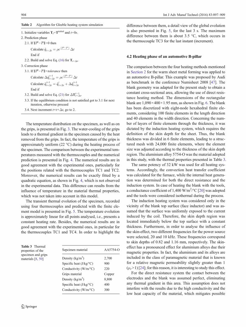
to try to guarantee a constant heating rate. The numericaltemperature Tc, evaluated in the position of the thermocoupleTC1, was compared with a pre-defined temperature Tp, inorder to define the vector of heat generation using thepredictor/corrector algorithm (Table 2). This pre-defined tem-perature Tp was calculated in each time instant, based on theprescribed heating rate.

The grips of the Gleeble system were water-cooled dur-ing the heating process. In the present study, the heat loss tothe grips was modelled applying a high convection coeffi-cient in the top surface of the grip, which was a procedurealso adopted by Kardoulaki et al. [46]. The value of theconvection coefficient used was 1,000 W/m2/°C, with atemperature of 22 °C for the T∞ in Eq. (4). Additionally,the heat loss by convection to the environment was takeninto account using a convection coefficient of 40 W/m2/°Cand air temperature of 22 °C, as suggested in [26]. Thethermal properties of the aluminium alloy 5754-O and thecopper grips were assumed as temperature-independent andisotropic and are given in Table 3.

(a) (b)

TC4TC3TC2TC1

bLc

L0

Fig. 1 Direct resistance heatingusing a Gleeble system: (a)experimental set-up; (b) geometryof the specimen (L0=40mm, b=10mm and Lc=80mm)

TC4

Water coolingh=1000 W/m2/°CT=22°C

Symmetry planx=0

Symmetry planz=0

SpecimenAA5754-O

GripCopper

Heat losses to the environmenth=40 W/m2/°CT=22°C

Symmetry plany=0

TC3

TC2

TC1

x

y z

Fig. 2 Finite element model ofthe tensile specimen and the gripused in the Gleeble system (oneeighth)

Int J Adv Manuf Technol (2016) 83:897–909 903

The temperature distribution on the specimen, as well as onthe grips, is presented in Fig. 3. The water-cooling of the gripsleads to a thermal gradient in the specimen caused by the heatremoved from the grips. In fact, the temperature of the grips isapproximately uniform (22 °C) during the heating process ofthe specimen. The comparison between the experimental tem-peratures measured with the thermocouples and the numericalprediction is presented in Fig. 4. The numerical results are ingood agreement with the experimental ones, particularly forthe positions related with the thermocouples TC1 and TC2.Moreover, the numerical results can be exactly fitted by aquadratic equation, as shown in Fig. 4, which is not observedin the experimental data. This difference can results from theinfluence of temperature in the material thermal properties,which was not taken into account in this model.

The transient thermal evolution of the specimen, recordedusing four thermocouples and predicted with the finite ele-ment model is presented in Fig. 5. The temperature evolutionis approximately linear for all points analysed, i.e., presents aconstant heating rate. Besides, the numerical results are ingood agreement with the experimental ones, in particular forthe thermocouples TC1 and TC4. In order to highlight the

difference between them, a detail view of the global evolutionis also presented in Fig. 5, for the last 3 s. The maximumdifference between them is about 3.5 °C, which occurs inthe thermocouple TC3 for the last instant (increment).

4.2 Heating phase of an automotive B-pillar

The comparison between the four heating methods mentionedin Section 2 for the warm sheet metal forming was applied toan automotive B-pillar. This example was proposed by Audias benchmark in the conference Numisheet 2008 [47]. Theblank geometry was adapted for the present study to obtain aconstant cross-sectional area, allowing the use of direct resis-tance heating method. The dimensions of the rectangularblank are 1,090×400×1.95mm, as shown in Fig. 6. The blankhas been discretized with eight-node hexahedral finite ele-ments, considering 100 finite elements in the length directionand 40 elements in the width direction. Concerning the num-ber of layers of finite elements through the thickness, it wasdictated by the induction heating system, which requires thedefinition of the skin depth for the sheet. Thus, the blankthickness was divided in 6 finite elements, leading to a struc-tured mesh with 24,000 finite elements, where the elementsize was adjusted according to the thickness of the skin depthregion. The aluminium alloy 5754-Owas the material adoptedin this study, with the thermal properties presented in Table 3.

The same potency of 32 kW was used for all heating sys-tems. Accordingly, the convection heat transfer coefficientwas calculated for the furnace, while the internal heat genera-tion was determined for both the direct resistance and theinduction system. In case of heating the blank with the tools,a conductance coefficient of 1,400W/m2/°C [20] was adoptedand the tools were considered isothermal during the process.

The induction heating system was considered only in thevicinity of the blank top surface (face inductor) and was as-sumed that the surface was uniformly exposed to the currentinduced by the coil. Therefore, the skin depth region waslocated immediately below the top surface with a constantthickness. Furthermore, in order to analyse the influence ofthe skin-effect, two different frequencies for the power sourcewere selected, 20 and 10 kHz. These frequencies correspondto skin depths of 0.82 and 1.16 mm, respectively. The skin-effect has a pronounced effect for aluminium alloys due theirmagnetic properties. In fact, the aluminium and its alloys areincluded in the class of paramagnetic material that is knownfor a relative magnetic permeability slightly greater than 1(μr>1) [24]; for this reason, it is interesting to study this effect.

For the direct resistance system the contact between theelectrodes and the blank was assumed perfect, eliminatingany thermal gradient in this area. This assumption does notinterfere with the results due to the high conductivity and thelow heat capacity of the material, which mitigates possible

Table 3 Thermalproperties of thespecimen and gripsmaterials [8, 50]

Sepcimen material AA5754-O

Density (kg/m3) 2,700

Specific heat (J/kg/°C) 900

Conductivity (W/m/°C) 220

Grips material Copper

Density (kg/m3) 8,800

Specific heat (J/kg/°C) 400

Conductivity (W/m/°C) 300

Table 2 Algorithm for Gleeble heating system simulation

1. Initialize variables Tt=Tinitial and t=0s.

2. Prediction phase

2.1. If ‖Tp−Tc‖>0 then

Calculate q�

tþΔt ¼ ρc Tp−T cð Þ Δt

End if

2.2. Build and solve Eq. (16) for Tt+Δt.

3. Correction phase

3.1. If ‖Tp−Tc‖>tolerance then

CalculateΔq� iþ1tþΔt ¼ ρc Tp−T cð Þ Δt

Calculate q� iþ1tþΔt ¼ q

� itþΔt þΔq

� iþ1tþΔt

End if

3.2. Build and solve Eq. (21) for ΔTt+Δti+1 .

3.3. If the equilibrium condition is not satisfied got to 3.1 for nextiteration, otherwise proceed

3.4. Next increment t=t+Δt, go to 2.

904 Int J Adv Manuf Technol (2016) 83:897–909

thermal gradients resulting from the defective contact betweenthe blank and the electrodes.

Since the induction and direct resistance heating processesare typically carried out at ambient temperature, the finiteelement model considers the heat loss by convection to theenvironment. A convection coefficient of 40 W/m2/°C and atemperature of 22 °C were used. The heating of the blankinside the forming tools requires a more complex approachto model the convection phenomenon. Figure 7 presents aschematically representation of the tools geometry, showingthe region delimited by the tools, which is subject to heat losesfor the environment. Although this interior area is identical forthe top and bottom surface of the blank, the heat loss rates aredifferent due to the favourable situation of the top surface forbuoyancy force moving the air from the surface. Thus, differ-ent convection coefficients were determined for the top andbottom surface of the blank, based on the empirical equationsdetermined by Lloyd et al. [48]:

htop ¼ 0:15RaL13

k

L; ð27Þ

hbott ¼ 0:52RaL15

k

L; ð28Þ

where RaL is the Rayleigh number calculated for the proper-ties of the air evaluated at 22 °C (temperature assumed for theenvironment). The convection coefficients determined withEqs. (27) and (28) were 9.06 W/m2/°C for the top surfaceand 2.31 W/m2/°C for the bottom surface.

4.2.1 Results and discussion

Figure 8 presents the thermal response of the blank for eachheating process (furnace, induction and direct resistance sys-tems). Since a uniform temperature field was observed alongthe process for these three heating systems, the temperatureevolution was collected on the centre of the blank (point B inFig. 6). This is a consequence of the high thermal conductivityand low heat capacity of the aluminium blank. The resultsconfirm that the use of a furnace in these conditions is themost time consuming option, due to the heat transfer mecha-nism inherent to this heating system. The other two systemsare more efficient, but it has to be highlighted that direct

0

30

60

90

120

150

180

210

0 2 4 6 8 10 12 14

Tem

pera

ture

[°C

]

Time [s]

TC1 - ExpTC1 - NumTC2 - ExpTC2 - NumTC3 - ExpTC3 - NumTC4 - ExpTC4 - Num

Fig. 5 Temperature evolution measured experimentally (thermocouples)and calculated with the numerical model

150

160

170

180

190

200

210

-20 -15 -10 -5 0 5 10 15 20

Tem

pera

ture

[°C

]

Posiiton along x [mm]

Polynomial fitExpNum

Fig. 4 Comparison between experimental and numerical temperaturedistributions along the specimen length

Fig. 3 Temperature distributionin the specimen and grips for theheating process using a Gleeblesystem (complete model)

Int J Adv Manuf Technol (2016) 83:897–909 905

resistance presented the highest heating rate. The decline onefficiency of the induction system was caused by the increaseof frequency. The skin-effect is an important drawback inher-ent to the system and its control is important to minimize theloss of efficiency. It has to be mentioned that the heat loss forthe environment in the direct resistance and induction systemswas relative less importance than the heat supplied by thesystems, causing irrelevant losses for the system efficiency.

The distribution of temperature on the blank heated by theforming tools is presented in Fig. 9 for different time instants.As expected, the area of the blank in contact with the formingtools shows the higher temperatures. This is highlighted inFigs. 10 and 11, which present the temperature distributionfor the nodes located in section AA and section BB (Fig. 6),respectively. The area which was not in contact with the toolsshows the lowest temperatures, revealing that the heat lossesfor the environment are very important for this specificheating method. The temperature evolution for the points A,B, C and D (see Fig. 6) is presented in Fig. 12. The tempera-ture difference between the points C and A, evaluated in thefinal instant of the process when the stationary temperaturedistribution was achieved, was about 30 °C. Therefore, when

using this heating method it can be important to model theheating phase, in order to take into account the thermal gradi-ents observed. However, these thermal gradients can be ex-perimentally avoided if the process elapses with the entireblank isolated in a temperature-controlled environment.

Fig. 9 Distribution of the blank temperature predicted by the numericalmodel at different instants: a 2 s; b 4 s; c 42 s; d 122 s

0

50

100

150

200

250

300

0 20 40 60 80 100

Tem

pera

ture

[°C

]

Time [s]

Furnace 32kWDirect Resistance 32kWInduction 32kW-20kHzInduction 32kW-10kHz

Fig. 8 Comparison of the blank temperature evolution for differentheating processes: furnace, direct resistance system and inductionsystem with different frequencies

Fig. 7 Scheme of the area of the forming tools (die and blank-holder) incontact with the blank during the heating phase

A

A

B B

Point A

Point B Point CPoint D

Blank-holder

Blank

Fig. 6 Scheme of the modified blank shape used in the automotive B-pillar forming

906 Int J Adv Manuf Technol (2016) 83:897–909

4.2.2 Temperature distribution after the transport for externalheating methods

After the heating phase, the external heating methods require asubsequent transport phase from the heating equipment to thepress. This transport operation is not standardized and has aduration that depends of the set-up. Hence, it is interesting toverify the response of the heated blank to boundary conditionsexpected for this phase. For numerical simulation of the trans-port phase it was only considered the heat loss for the envi-ronment, neglecting any possible losses resulting from thecontact with the carrying tools. Thus, only a convection termwas considered for the boundary conditions. A convectionheat transfer coefficient of 40 W/m2/°C and a temperature of22 °Cwere assumed in order to simulate the air-cooling effect.

The heating and the transport phase were performed in asingle simulation process. This allowed to consider the tem-perature field of the heating phase as initial condition for thetransient thermal problem of the transport phase. The temper-ature gradients within the blank may be neglected, because theconduction resistance is small compared with the resistance to

heat transfer between the blank and the surrounding air. Basedon that, the temperature on the blank can be determined usingthe lumped capacitance method [49], which allows the deter-mination of the temperature within the blank:

T ¼ T∞ þ T i−T∞ð Þexp −hconvAs

ρcVt

� �; ð29Þ

based on the initial temperature Ti and on the area of the blanksurface exposed to the air As.

The evolution of blank temperature only for the transportphase is presented in Fig. 13, evaluated by finite elementmethod (numerical) and by Eq. (29) (analytical). The numer-ical results are in very good agreement with the analyticalones, which indicate a reduction of about 13 °C after 7 s ofexposure time to the conditions aforementioned. This revealsthat heat losses during the transport process should be consid-ered, when a material with temperature-dependent propertiesis considered in a forming process simulation. The assumptionof imposed temperature as the exact temperature before thedeformation process can be a source of inaccuracies,compromising posterior results.

0

150

300

450

600

750

900

0

30

60

90

120

150

180

210

240

0 20 40 60 80 100 120 140

Initi

al te

mpe

ratu

re [°

C]

Tem

pear

ture

[°C

]

Transport time [s]

NumericalAnalyticalInitial Temp.

Fig. 13 Decreasing blank temperature during the transport phase andinitial temperature required to assure a final temperature of 250 °C afterthe transport phase

0

50

100

150

200

250

300

0 30 60 90 120 150 180 210 240

Tem

pera

ture

[°C

]

Time [s]

Point A

Point B

Point C

Point D

Fig. 12 Temperature evolution for the points a, b, c and d illustrated inFig. 6

0

50

100

150

200

250

300

0 200 400 600 800 1000

Tem

pera

ture

[°C

]

Position along x [mm]

t=10s t=30s t=50s t=75s

t=100s t=150s t=200s

Fig. 11 Evolution of the blank temperature predicted by the numericalmodel for the section BB

0

50

100

150

200

250

300

0 50 100 150 200 250 300 350 400

Tem

pera

ture

[°C

]

Position along y [mm]

t=10st=30st=50st=75st=100st=150st=200s

Fig. 10 Evolution of the blank temperature predicted by the numericalmodel for the section AA

Int J Adv Manuf Technol (2016) 83:897–909 907

In the warm forming process set-up, this heat loss could becompensated with an overheating. However, it has to be men-tioned that the increase of temperature during the heatingphase can be detrimental for the material. Therefore, it wouldbe necessary to determine accurately the precise time for thetransport phase, before calculating the overheating needed toachieve the exact warm forming temperature, for the timeinstant before the start of the deformation. In order to balancethe heat loss during the transport phase, the initial temperatureto assure 250 °C after the transport phase can be determined.This can be done by solving Eq. (29) for the variable Ti. Theinitial temperature to assure 250 °C after the transport phase isalso presented in Fig. 13, taking into account the transporttime.

5 Conclusions

This paper presents a summary of a finite element formula-tion, developed to simulate the heating and transport phasesinvolved in warm sheet metal forming processes. An analysisof the state-of-art heating methods was presented, includingtemperature distribution and the heating time necessary toachieve the warm forming temperature. This analysis revealsabrupt thermal gradients for the blank heating inside the toolsin the end of the process, which are usually ignored in theforming simulation process. For the external heating methods,the furnace was the most time-consuming process. However,if the objective is to achieve a uniform temperature thisheating system as well as the others external systems are thebest options. The transport phase for the external heatingmethods was also studied revealing that high heat losses occurin the initial instants of this phase, which could be balancedwith an overheating. Nevertheless, a preliminary analysis isnecessary to evaluate possible detrimental effects on the ma-terial, resulting from the overheating.

A novel algorithm for the prediction of thermal fields ob-served in a specimen tested on Gleeble system was presented.The results from the finite element model were compared withexperimental results. Despite the several simplifications as-sumed in the model, the numerical and experimental resultswere found to be in agreement.

Acknowledgments The authors gratefully acknowledge the financialsupport of the Portuguese Foundation for Science and Technology (FCT)under project PTDC/EMS-TEC/1805/2012 and by FEDER fundsthrough the program COMPETE—Programa Operacional Factores deCompetitividade, under the project CENTRO-07-0224-FEDER-002001(MT4MOBI). The authors would like to thank Prof. A. Andrade-Camposfor helpful contributions on the development of the finite element codepresented in this work.

References

1. González Palencia JC, Furubayashi T, Nakata T (2012) Energy useand CO2 emissions reduction potential in passenger car fleet usingzero emission vehicles and lightweight materials. Energy 48:548–565. doi:10.1016/j.energy.2012.09.041

2. Hirsch J (2014) Recent development in aluminium for automotiveapplications. Trans Nonferrous Met Soc Chin 24:1995–2002. doi:10.1016/S1003-6326(14)63305-7

3. Kulekci MK (2007) Magnesium and its alloys applications in au-tomotive industry. Int J Adv Manuf Technol 39:851–865. doi:10.1007/s00170-007-1279-2

4. Toros S, Ozturk F, Kacar I (2008) Review of warm forming ofaluminum-magnesium alloys. J Mater Process Technol 207:1–12.doi:10.1016/j.jmatprotec.2008.03.057

5. Kurukuri S, van den Boogaard AH, Miroux A, Holmedal B (2009)Warm forming simulation of Al–Mg sheet. JMater Process Technol209:5636–5645. doi:10.1016/j.jmatprotec.2009.05.024

6. Ghosh M, Miroux A, Werkhoven RJ et al (2014) Warm deep-drawing and post drawing analysis of two Al–Mg–Si alloys. JMater Process Technol 214:756–766. doi:10.1016/j.jmatprotec.2013.10.020

7. Abedrabbo N, Pourboghrat F, Carsley J (2007) Forming ofAA5182-O and AA5754-O at elevated temperatures using coupledthermo-mechanical finite element models. Int J Plast 23:841–875.doi:10.1016/j.ijplas.2006.10.005

8. Laurent H, Coër J, Manach PY et al (2015) Experimental and nu-merical studies on the warm deep drawing of an Al–Mg alloy. Int JMech Sci 93:59–72. doi:10.1016/j.ijmecsci.2015.01.009

9. Grèze R, Manach PY, Laurent H et al (2010) Influence of the tem-perature on residual stresses and springback effect in an aluminiumalloy. Int J Mech Sci 52:1094–1100. doi:10.1016/j.ijmecsci.2010.04.008

10. Coër J, Manach PY, Laurent H et al (2013) Piobert–Lüders plateauand Portevin–Le Chatelier effect in an Al–Mg alloy in simple shear.Mech Res Commun 48:1–7. doi:10.1016/j.mechrescom.2012.11.008

11. Ghaffari Tari D, Worswick MJ, Winkler S (2013) Experimentalstudies of deep drawing of AZ31B magnesium alloy sheet undervarious thermal conditions. J Mater Process Technol 213:1337–1347. doi:10.1016/j.jmatprotec.2013.01.028

12. Hung N, Marion M (2012) Improved formability of aluminum al-loys using laser induced hardening of tailored heat treated blanks.Phys Procedia 39:318–326. doi:10.1016/j.phpro.2012.10.044

13. Larsson L (2005) Warm sheet metal forming with localized in-toolinduction heating. Lund University

14. Hasanuzzaman M, Rahim NA, Hosenuzzaman M et al (2012)Energy savings in the combustion based process heating in indus-trial sector. Renew Sustain Energy Rev 16:4527–4536. doi:10.1016/j.rser.2012.05.027

15. Zhao PJ, Chen ZH, Dong CF (2014) Failure analysis of warmstamping ofmagnesium alloy sheet based on an anisotropic damagemodel. J Mater Eng Perform 23:4032–4041. doi:10.1007/s11665-014-1214-2

16. Harrison NR, Ilinich A, Friedman PA, et al. (2013) Optimization ofhigh-volume warm forming for lightweight sheet

17. Menezes LF, Teodosiu C (2000) Three-dimensional numerical sim-ulation of the deep-drawing process using solid finite elements. JMater Process Technol 97:100–106. doi:10.1016/S0924-0136(99)00345-3

18. Oliveira MC, Alves JL, Menezes LF (2008) Algorithms and strat-egies for treatment of large deformation frictional contact in thenumerical simulation of deep drawing process. Arch ComputMethods Eng 15:113–162. doi:10.1007/s11831-008-9018-x

908 Int J Adv Manuf Technol (2016) 83:897–909

19. Kolleck R, Veit R, Merklein M et al (2009) Investigation on induc-tion heating for hot stamping of boron alloyed steels. CIRP Ann -Manuf Technol 58:275–278. doi:10.1016/j.cirp.2009.03.090

20. Takuda H, Mori K, Masuda I et al (2002) Finite element simulationof warm deep drawing of aluminium alloy sheet when accountingfor heat conduction. J Mater Process Technol 120:412–418. doi:10.1016/S0924-0136(01)01180-3

21. Lade J, Banoth BN, Gupta AK, Singh SK (2014) Metallurgicalstudies of austenitic stainless steel 304 under warm deep drawing.J Iron Steel Res Int 21:1147–1151. doi:10.1016/S1006-706X(14)60197-7

22. Koh Y, Kim D, Seok D et al (2015) Characterization of mechanicalproperty of magnesium AZ31 alloy sheets for warm temperatureforming. Int J Mech Sci 93:204–217. doi:10.1016/j.ijmecsci.2015.02.001

23. Krajewski PE (2001) Elevated temperature forming of sheet mag-nesium alloys

24. Rudnev V, Loveless D, Cook RL, Black M (2002) Handbook ofinduction heating. CRC Press, Boca Raton

25. Codrington J, Nguyen P, Ho SY, Kotousov A (2009) Inductionheating apparatus for high temperature testing of thermo-mechanical properties. Appl Therm Eng 29:2783–2789. doi:10.1016/j.applthermaleng.2009.01.013

26. Takuda H, Morishita T, Kinoshita T, Shirakawa N (2005)Modelling of formula for flow stress of a magnesium alloy AZ31sheet at elevated temperatures. J Mater Process Technol 164–165:1258–1262. doi:10.1016/j.jmatprotec.2005.02.034

27. Pellegrini D, Ghiotti A, Bruschi S (2011) Effect of warm formingconditions on AZ31B flow behaviour and microstructural charac-teristics. Int J Mater Form 4:155–161. doi:10.1007/s12289-010-1025-4

28. Mori K (2012) Smart hot stamping of ultra-high strength steel parts.Trans Nonferrous Met Soc Chin 22:s496–s503. doi:10.1016/S1003-6326(12)61752-X

29. Mori K, Maki S, Tanaka Y (2005) Warm and hot stamping of ultrahigh tensile strength steel sheets using resistance heating. CIRPAnn- Manuf Technol 54:209–212. doi:10.1016/S0007-8506(07)60085-7

30. Das S, Barekar N, El Fakir O et al (2015) Influence of intensivemelt shearing on subsequent hot rolling and the mechanical prop-erties of twin roll cast AZ31 strips. Mater Lett 144:54–57. doi:10.1016/j.matlet.2015.01.017

31. Coër J, Bernard C, Laurent H et al (2011) The effect of temperatureon anisotropy properties of an aluminium alloy. Exp Mech 51:1185–1195. doi:10.1007/s11340-010-9415-6

32. Doege E, Dröder K (2001) Sheet metal forming of magnesiumwrought alloys—formability and process technology. J MaterProcess Technol 115:14–19. doi:10.1016/S0924-0136(01)00760-9

33. Palumbo G, Sorgente D, Tricarico L et al (2007) Numerical andexperimental investigations on the effect of the heating strategy and

the punch speed on the warm deep drawing of magnesium alloyAZ31. J Mater Process Technol 191:342–346. doi:10.1016/j.jmatprotec.2007.03.095

34. Lee YS, Kim MC, Kim SW et al (2007) Experimental and analyt-ical studies for forming limit of AZ31 alloy on warm sheet metalforming. J Mater Process Technol 187–188:103–107. doi:10.1016/j.jmatprotec.2006.11.118

35. Bathe KJ (1996) Finite element procedures. Prentice-Hall,Englewood Cliffs

36. Rodrigues JMC, Martins PAF (2002) Finite element modelling ofthe initial stages of a hot forging cycle. Finite Elem Anal Des 38:295–305. doi:10.1016/S0168-874X(01)00065-8

37. Zhu J, Taylor ZRL, Zienkiewicz OC (2005) The finite elementmethod: its basis and fundamentals. Butterworth-Heinemann

38. Hughes TJR (2012) The finite element method: linear static anddynamic finite element analysis. Courier Corporation

39. Madoliat R, Ghasemi A (2008) Inverse finite element formulationsfor transient heat conduction problems. Heat Mass Transf 44:569–577. doi:10.1007/s00231-007-0270-7

40. Vaz Jr M (2000) Simulação de problemas de acoplamentotermomecânico

41. Menezes LF, Neto DM, Oliveira MC, Alves JL (2011) Improvingcomputational performance through HPC techniques: case studyusing DD3IMP in-house code. AIP Conf Proc 1353:1220–1225.doi:10.1063/1.3589683

42. Andrade-Campos A, da Silva F, Teixeira-Dias F (2007) Modellingand numerical analysis of heat treatments on aluminium parts. Int JNumer Methods Eng 70:582–609. doi:10.1002/nme.1905

43. Xing HL, Makinouchi A (2002) FE modeling of thermo-elasto-plastic finite deformation and its application in sheet warm forming.Eng Comput 19:392–410. doi:10.1108/02644400210430172

44. Stratton JA (1941) Electromagnetic theory. McGraw-Hill, NewYork

45. Zinn S, Semiatin SL (1988) Elements of induction heating46. Kardoulaki E, Lin J, Balint D, Farrugia D (2014) Investigation of

the effects of thermal gradients present in Gleeble high-temperaturetensile tests on the strain state for free cutting steel. J Strain AnalEng Des 49:521–532. doi:10.1177/0309324714531950

47. Numisheet 2008 (2008) The Numisheet Benchmark Study,Benchmark Problem BM03

48. Lloyd JR, Moran WR (1974) Natural convection adjacent to hori-zontal surface of various planforms. J Heat Transfer 96:443–447

49. Incropera FP (2011) Fundamentals of heat andmass transfer.Wiley,Canada

50. Kim HS, Koç M (2008) Numerical investigations on springbackcharacteristics of aluminum sheet metal alloys in warm formingconditions. J Mater Process Technol 204:370–383. doi:10.1016/j.jmatprotec.2007.11.059

Int J Adv Manuf Technol (2016) 83:897–909 909