numerical analysis of podded and steering systems using a ... · propeller-induced velocities...

Numerical Analysis of Podded and Steering Systems Using a Velocity Based Source Boundary Element Method with Modified Trailing Edge Alexander S. Achkinadze1, Aage Berg2, Vladimir I. Krasilnikov3 and Ivan E. Stepanov4

ABSTRACT

This paper describes an improved velocity based source boundary element method (BEM) as applied to modeling of podded propellers and propeller/rudder systems. The distinctive feature of the present method consists in the direct satisfaction of the Kutta-Joukowski condition on the additional Kutta panel constructed behind the realistic blade trailing edge when defining the unknown doublet strength. This Modified Trailing Edge (MTE) is also used as a tool for the approximate accounting for viscous and related effects on circulation. The integrated propulsive/steering system is simulated within the potential frameworks using the velocity field iterations method and quasi-steady approach, which assumes the simulation of propeller in a spatially varying flow field while pod and strut(/rudder) are considered in a circumferentially averaged flow field. The developed method is applied for calculation of rudder behind the operating propeller and podded units of different arrangement tested at MARINTEK (Norwegian Marine Technology Research Institute). The results of the measurements and theory/experiment comparisons are discussed.

1 Professor, D.Tech.Sc., Dept. of Ship Hydrodynamics, SMTU, St Petersburg, Russia 2 Senior Research Engineer, MSc, Nav.Arch., Div. of Ship Performance, MARINTEK, Trondheim, Norway 3 Research Scientist, PhD, Div. of Ship Performance, MARINTEK, Trondheim, Norway 4 Research Engineer, PhD, Dept. of Ship Hydrodynamics, SMTU, St Petersburg, Russia

INTRODUCTION In recent years pod systems have become an intensively developing type of marine propulsors, which attracts attention of the both designers and researchers. The power output of full-scale arrangements has increased significantly and according to (Friesch, 2001) varies now within the range from 5 to 30 MW per unit. The variety of pod arrangements also increases and along with single pulling and pushing devices (Hämäläinen and Heerd, 2001) the alternative two-staged conceptions are applied, for example, such as pushing thruster with contra-rotating propellers (CRP), shaft arrangement with additional contra-rotating (CR) pod drive, Siemens-Schottel tandem unit with for/aft location of blade-row stages (Kurimo et.al., 1997), (Friesch, 2001). Nowadays pod systems are used not only on cruise vessels and arctic tankers, but also on semi-submersible heavy lift vessels, chemical tankers and floating platforms.

In spite of that the experimental studies on podded propellers have been started quite long ago only a few experimental results can be found in the open publications. The extensive investigation in cavitation behavior, vibration and acoustics of single-screw pushing and pulling units and Siemens-Schottel (tandem) and CRP arrangements have been performed in the cavitation tunnel at HSVA and the results have been presented in (Friesch, 2001). The extremely interesting results on maneuvering forces on the different types of pod systems including single-screw pushing/pulling units and tandem propulsor have been obtained at Technical University of Gdansk and published in (Szantyr, 2001). More and more researchers address their efforts to numerical simulation of pod and multi-staged systems. Mathematical tools employed for these purposes vary from purely potential lifting surface (Yang et.al., 1992), (Hughes and Kinnas, 1993), (Chun et.al., 2001) and boundary element (Ghassemi and Allievi, 1999)

Proc. of the Propellers/Shafting '2003 Symp., SNAME - VA, USA - Sept 17-18, 2003

methods through coupled potential lifting-surface/RANS (Reynolds-Averaged Navier-Stokes) algorithms (Kerwin et.al., 1997), (Warren et.al., 2000), (Hsin et.al., 2002) and Euler solvers (Kinnas et.al., 2001) to direct RANS calculations (Sanchez-Caja et.al., 1999). A significant amount of experimental studies on pod propulsors (both commercial and research) has been carried out in the cavitation tunnel and towing tank at MARINTEK. The obtained results inspired the development of quite universal numerical tool capable to simulate the most widespread pod arrangements and provided the authors with a good basis for validation of their method. The analysis program is based on the original velocity-based BEM developed by the authors and applied earlier to the analysis of foils (Achkinadze and Krasilnikov, 2001), single propellers (Achkinadze and Krasilnikov, 2001a), and propeller/rudder systems (Achkinadze et.al., 2002). Numerical verification revealed an importance of improved corrections accounting for the viscous effects on circulation and propeller-induced velocity field. Since the interaction between the propulsor components is captured via mutually induced velocity fields, reliable prediction of propeller-induced velocities becomes especially important. The results of laser Doppler velocimetry (LDV) and Pito-Prandtl measurements in propeller wake have been used for the verification of velocity field algorithm. The first trial for the newly developed code was a case of conventional propeller/rudder arrangement and the algorithm of prediction of rudder surface pressure and rudder forces has been verified. The following validation work concerned the pod arrangements of different types such as pulling and pushing single-screw unit and CRP podded thruster. Prediction of open-water performance and maneuvering forces at different heading angles was in the focus of comparisons. The present paper describes the authors’ analysis method and illustrates the main results obtained during validation study. MAIN ASSUMPTIONS OF MODELING OF PROPULSOR USING THE POTENTIAL THEORY The two-staged podded propulsor is considered. Two blade rows can be located on the pod at the arbitrary sections along the pod length. The pod is considered as an axisymmetrical body and the origin of the global fixed coordinate system coincides with its midlength section. The unit has a strut, which is represented as a wing of quite arbitrary geometry (including twisted configuration) attached to the pod with its lower tip. The strut section profiles are also arbitrary. Naturally,

such a general formulation includes the case of conventional shaft arrangement with hub and the case of rudder behind propeller(s). There is no restriction imposed on blade row geometry. The fluid is assumed to be incompressible and inviscid and the velocity field irrotational everywhere except on the propeller blades and strut(/rudder) and their trailing vortex wakes. The blade rows and strut are simulated as lifting bodies while the pod is treated as a displacing body. The spatially varying inflow field due to hull is assumed to be prescribed in a number of sections at the sites of blade rows or – as it takes place very often in practical calculations – only in the blade row planes, and then it is considered as axially invariable. The system of correction factors is applied to take into account the effect of viscosity on propeller and strut forces and circulation obtained from the potential solution, and the effect of surface friction on propeller- and strut-induced velocity fields and forces on the pod. The interaction between the components of propulsor is taken into account through the mutually induced velocity fields (method of velocity field iterations). There are two principal assumptions made in this regard. First, the propeller-induced velocity field is always considered as circumferentially averaged while propellers themselves are treated in the non-homogeneous flow. The non-homogeneity comes from the prescribed inflow field and from the interaction between propellers and strut. Secondly, the hypothesis about penetrability of the bodies for trailing vortices is used. It implies that trailing vortices from propeller blades and strut freely penetrate through the bodies as if the letter would absent and do not experience any deformation. At the same time the kinematic boundary condition is strictly satisfied on the bodies. Along with the assumption about absence of the shed vortices in propeller and strut vortex wakes this formulation meets so-called quasi-steady approach, which is discussed below in more details. VELOCITY BASED BEM FOR PROPELLER AND STRUT(/RUDDER) Governing equations The flow field around lifting body can be described by the following vectors: VR – total relative velocity of fluid, VE – transferal velocity of the given point on the body surface, W – velocity induced by the body and the cavities, Vψ – inflow velocity. The listed vectors are related as follows (Kochin et al., 1963):

ER VVVWrrrr

+=+ ψ . (1)

a)

ML

MUV

SUFVS

SCAV

SWET

SV Ω

SLFVS

The general system of equations, which describe the flow, consists of the Euler equation and the continuity equation. The Euler equation is written below in the form by Gromeko-Lamb (Kochin et al., 1963):

pgradVWrotVVW

VWgradVVWgradt

VW

E

E

ρ1)()(

)(2

)()( 2

−=+×−+

−+⋅−+

+∂+∂′

ΨΨ

ΨΨΨ

rrrrr

rrrrrrr

, (2)

where p is the hydrodynamic pressure, which does not include the gravity forces, and the derivative

t∂∂′ /(...) is calculated in the coordinate system moving together with the body (for example, propeller-fixed coordinate system in the case of rotating blade row). Under the assumptions adopted above the continuity equation is expressed by the Laplace equation:

0=∆ϕ , (3) where ϕ is the absolute velocity potential. The problem about non-cavitating flow allows separate consideration of the dynamic (pressure and forces) and kinematic (potential, velocity) parts of the solution. Then the following Lagrange (or unsteady Bernoulli) identity solves equation (2) in the unsteady case:

( )2

)(*22

ERA

VVt

ghpp−

−∂∂′

−=+−ρϕ

ρρ , (4)

while the steady Bernoulli identity is valid for the steady flow. The latter is obtained from (4) if

0=∂∂′ tϕ . In this equation the absolute total pressure p* includes gravity forces, pA is the atmospheric pressure, h is the submergence of the considered point under free surface, ρ is the density of water and g is the gravitation constant. The following kinematic conditions have to be satisfied. Kinematic boundary condition (“no flow”) on the wetted body surface SWET:

WETR SonnV 0=⋅rr

. (5) Condition of vanishing of the absolute velocities in the infinity outside the vortex wake (for the 3D case):

0,1,2

>∞→ℜℜ

→+

κκψ atVW , (6)

where ℜ is the distance from the origin of the body-fixed coordinate system to the considered point. In the 2D problem the degree exponent is κ+1 . Additional kinematic condition on the Modified Trailing Edge (MTE):

MTEMTER SonnV 0=⋅rr

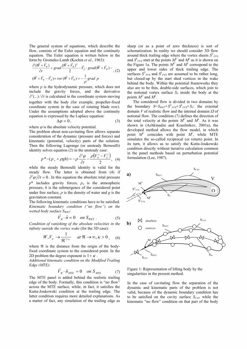
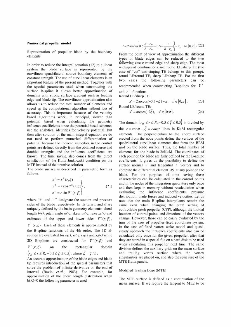
(7) The MTE panel is added behind the realistic trailing edge of the body. Formally, this condition is “no flow” across the MTE surface, while, in fact, it satisfies the Kutta-Joukowski condition at the trailing edge. The latter condition requires more detailed explanations. As a matter of fact, any simulation of the trailing edge as

sharp (or as a point of zero thickness) is sort of schematization. In reality we should consider 3D flow around thick trailing edge where the vortex sheets SU

FVS and SL

FVS start at the points MU and ML as it is shown on the Figure 1a. The points MU and ML correspond to the upper and lower sides of thick trailing edge. The surfaces SU

FVS and SLFVS are assumed to be rather long,

but closed-up by the start shed vortices in the wake behind the body. Within the potential frameworks they also are to be thin, double-side surfaces, which join to the notional vortex surface SV inside the body at the points MU and ML.

The considered flow is divided in two domains by the boundary S=SWET+SU

FVS+SLFVS+SV: the external

domain V of realistic flow and the internal domain Ω of notional flow. The condition (7) defines the direction of the total velocity at the points MU and ML. As it was shown in (Achkinadze and Krasilnikov, 2001a), the developed method allows the flow model, in which point MU coincides with point ML, while MTE simulates the so-called reciprocal (or return) point. In its turn, it allows us to satisfy the Kutta-Joukowski condition directly without iterative calculation common in the panel methods based on perturbation potential formulation (Lee, 1987). Figure 1: Representation of lifting body by the singularities in the present method. In the case of cavitating flow the separation of the dynamic and kinematic parts of the problem is not valid, because of the dynamic boundary condition has to be satisfied on the cavity surface SCAV while the kinematic “no flow” condition on that part of the body

b)

M

SCAV

SWET

SM SFVS

SMTE

sources

doublets

has to be taken off. However, the cavity domain is unknown beforehand and it is defined from the solution. The basic scheme of application of the authors’ method to cavitating flow problem was described in (Achkinadze and Krasilnikov, 2001), (Achkinadze and Krasilnikov, 2001a) and (Achkinadze et.al., 2002). The details of derivation of the main integral equation of the boundary value problem were considered in (Achkinadze and Krasilnikov, 2001a). Therefore, below we will discuss only the main features of this equation and give some important comments on its numerical implementation. The authors’ approach consists in obtaining an integral equation in the form of the Fredgolm’s integral equation of the 2nd kind, i.e. free of numerical singularities unlike the Fredgolm’s integral equation of the 1st kind, which is usually employed in the other velocity based BEMs. The main integral Green’s identity is applied to the both external V and internal Ω domains, and the sources of strength q are placed on the surface SQ=SWET+SCAV in order to simulate thickness effects, while the doublets of strength σ are placed on the surface

−+−+ ++++= LFVS

LFVS

UFVS

UFVSV SSSSSSσ in order to

simulate lift effects. As one can see from Figure 1b at such the transformation the vortex surfaces in the wake merge in one thin surface SFVS while the surface SV inside the body is reshaped into the mean surface SM. As a result we come to the main integral equation of no-cavitation problem:

( ) QE

SS

SonnVV

dsRnn

dsRn

qq

Q

rrr⋅−=

=

∂∂∂

+

∂∂

− ∫∫

ψ

σ

σππ

1411

41

2

2

. (8)

If the doublet strength σ is known then (8) is, indeed, the Fredgolm’s integral equation of the 2nd kind regarding unknown source strength q. The chordwise distribution of doublets can be arbitrary in the present method. When we consider the external flow domain it is not important how the doublets are distributed inside the body because of the only total circulation value defines lift effects. This circulation has to be calculated as an integral along the closed-up contour that intersects the surface Sσ at the point M on the MTE. In the present work the linear chordwise distribution of doublet strength has been adopted

( )( ) LETE

LETE

LE attrtr ξξξξξξξξσ ≤≤Γ−−

= ),(),,( . (9)

In the steady case the value of doublet strength at the trailing edge ),,( tr TEξσ conforms invariable in the wake behind the blade for the helix of given radius r down to the location of the conditional start shed vortex. In the unsteady problem the doublet strength in the wake is calculated as follows:

TEER

TE atV

trtr ξξξξξ

ξσξ

<≤−

−Γ= ),(),,( , (10)

where ξRV is the projection of total relative velocity on the ξ-direction defined at the trailing edge, and Eξ is the coordinate of the conditional start shed vortex, i.e. far boundary of the wake domain in the numerical integration procedure. The formula (10) follows from the Tomson theorem, which asserts the conformation of circulation along the closed-up fluid contour, which consists of the same particles, in the ideal incompressible flow with no mass forces (Kochin et al., 1963). For the practical implementation the main equation (8) has been rewritten in terms of vorticity instead of doublets using the Biot-Savart formula and the identity between vortex and doublet strengths (Artyushkov et.al., 1988)

σγ σ gradn ×=rr

, (11) where nσ is the normal to surface Sσ, γr is the surface vortex strength. It yields

[ ]

[ ] ( ) MTEQEL

L

SS

SSonnVVR

nRld

dsR

nRdsR

Rnqq

Q

+⋅−=×⋅Γ

+

×⋅+

⋅+

∫

∫∫

rrrrrr

rrrrr

ψ

σ

σ

π

γππ

3

33

41

41

41

2 . (12)

The last item in the left-hand part of (12) comes from the Biot-Savart formula in the case when σ (or γ) function has “jumps” or non-zero values on the boundaries of the surface Sσ (Kochin et al., 1963), (Artyushkov et al., 1988). For instance, it takes place at the root section of propeller blade if hub circulation is non-zero. Quasi-steady formulation The realistic velocity field, in which the propeller operates, is spatially and time varying, i.e. the inflow vector has to be written as follows

),,,( 000 trxVV θΨΨ =rr

, (13) where index “0” denotes the global fixed coordinate system, and t is the time. The circumferential non-homogeneity of the inflow is caused by a number of effects such as non-uniform hull wake in the site of propeller (which is assumed to be nominal as it has been mentioned above), non-zero heading angle of the pod drive (or shaft inclination) and interaction between propeller and strut(/rudder). In order to substitute this velocity field in the equation (12) we have to write it in the coordinate system fixed on propeller. The time parameter and the blade turn angle θP are connected through the identity

Ω= /Pt θ , (14)

where Ω is the propeller rotational speed. Thus, the inflow velocity field can be represented in the propeller-fixed coordinate system as follows:

)/,,,( Ω+= ΨΨ PPrxVV θθθrr

, (15) and, consequently, the unknown source and doublet strengths also become time-dependent, or angular-dependent in the given formulation. Numerically it means that the both matrices of influence coefficient (left-hand parts of (12)) and inflow field (right-hand parts of (12)) change with blade turn angle θP, and the solution of the integral equation should be performed in a step-wise manner at the given number of angular positions. The angular-dependent portion of the influence coefficients comes from the shed vorticity, which is a result of circumferential variation of circulation Γ. The identity for the shed vortex strength in propeller wake follows from the equation (10):

TEER

TE

Rr at

dt

Vtrd

Vξξξ

ξξ

γξ

ξ≤≤

−−Γ

−=

,1 . (16)

Thus, we have all the equations necessary to solve the unsteady problem. However, the first iteration can be obtained using a so-called quasi-steady approach, which assumes the invariable matrix of influence coefficients at angular-dependent right-hand parts. In fact, quasi-steady solution is always the first step in treatment of the unsteady problem, and in many cases it allows satisfactory precision, for instance, when defining the integral performance such as maneuvering forces. The quasi-steady pressure distribution is defined from the Lagrange identity (4), where the time derivative of absolute velocity potential ϕ is calculated in the propeller-fixed coordinate system. In the velocity based BEM after solution of the main integral equation we have values of induced velocities at the control points on the blade surface, but do not have values of potential. Therefore, ϕ is to be calculated in addition. It can be easily done through the representation of the total ϕ as a sum of the propeller-induced velocity (perturbation) potential and the inflow velocity potential

ψϕϕϕ += W , (17) and the following estimation of the time derivative for each of these parts separately. The propeller-induced velocity potential is defined through the source and doublet strengths obtained from the solution as follows

∫∫⋅

+−=σ

σππ

ϕSS

W dsR

RndsRq

Q

341

41

rr

. (18)

Let us note that the sign of the second item in this identity is caused by the adopted direction of the normal to the surface Sσ (it is positive when directed

from the pressure side to the suction side). After that the derivative can be calculated through the discrete values of potential that correspond to the calculated blade angular positions

11

11 ),,(),,(

),,(),,(

−+

−+

−

−=

=∂

∂′Ω=

∂

∂′

ip

ip

ip

ip

p

ipWpW

rr

rt

r

θθ

θξϕθξϕ

θθξϕθξϕ

. (19)

In order to find the second part of the time derivative of ϕ caused by the inflow velocity the following identity can be employed (Kochin et.al., 1963):

tyVzVVV

t zyx ∂

∂+Ω+Ω−=

∂

∂′ ψψψψ

ψ ϕϕ. (20)

As one can see this formula connects the time derivatives of potential calculated in the propeller-fixed (moving and rotating) and global fixed coordinate systems. In the case of prescribed wake field, which does not depend upon time, the last item in (20) is zero while all the other items are known. Another principal assumption of quasi-steady approach concerns the velocity fields, which are used when modeling the interaction between the components of propulsor (pod, rudder and blade rows). As it has been mentioned above the procedure of velocity field iterations is used in the present method. In the general case of two-staged podded propulsor the calculation starts with the analysis of pod body in uniform flow of given advance speed. The axisymmetric, axially and radially varying pod-induced velocity field is transferred into the propeller solver where it is added with nominal hull wake, which can be prescribed as in the propeller plane as in a number of sections along the propeller axis if such information is available (for each of blade-row stages separately). The quasi-steady analysis of propellers is performed in these velocity fields. The iterations between the blade rows form the 0-level (internal) cycle of the iteration procedure, and the mutually induced velocity fields due to propellers are considered as mean (circumferentially averaged). The total velocity field induced by the both blade-row stages is returned back on the 1-level (intermediate) cycle to repeat the analysis of pod body. The total velocity field, which is obtained as a sum of pod-induced and propeller-induced velocity fields, is the input field for the strut(/rudder) solver. Strut(/rudder) is always considered in an axisymmetric flow, i.e. in steady formulation. At the same time the flow field induced by the strut(/rudder) is circumferentially varying and it is used at the next step of the 2-level (external) cycle as the input information for the analysis of pod and blade rows.

Numerical propeller model Representation of propeller blade by the boundary elements In order to reduce the integral equation (12) to a linear system the blade surface is represented by the curvilinear quadrilateral source boundary elements of constant strength. The use of curvilinear elements is an important feature of the present method. Together with the special parameters used when constructing the surface B-spline it allows better approximation of domains with strong surface gradient such as leading edge and blade tip. The curvilinear approximation also allows us to reduce the total number of elements and speed up the computational algorithm without loss of accuracy. This is important because of the velocity based algorithms work, in principal, slower than potential based when calculating the geometry influence coefficients since the potential based schemes use the analytical identities for velocity potential. But then after solution of the main integral equation we do not need to perform numerical differentiation of potential because the induced velocities in the control points are defined directly from the obtained source and doublet strengths and the influence coefficients are known. The time saving also comes from the direct satisfaction of the Kutta-Joukowski condition on the MTE instead of the iterative solution. The blade surface is described in parametric form as follows

=

=

=

±±

±±

±±

),(sin

),(cos

),(

ξθ

ξθ

ξ

rrz

rry

rxx

, (21)

where “+” and “−” designate the suction and pressure sides of the blade respectively. In its turn x and θ are uniquely defined by the basis geometry elements: chord length b(r), pitch angle ϕ(r), skew cS(r), rake xR(r) and ordinates of the upper and lower sides ),( ξrY + ,

),( ξrY − . Each of these elements is approximated by the B-spline functions of the 4th order. The 1D B-splines are evaluated for b(r), ϕ(r), cS(r) and xR(r) while 2D B-splines are constructed for ),( ξrY + and

),( ξrY − on the rectangular domain

5.0~5.0; ≤≤−≤≤ ξRrrH , where b/~ξξ = .

An accurate approximation of the blade edges and blade tip requires introduction of the special parameters that solve the problem of infinite derivative on the end of interval (Bavin et.al., 1983). For example, for approximation of the chord length distribution when b(R)=0 the following parameter is used

[ ]ππ ;0,5.05.0arccos2 ∈−

−

−−−+

= trR

rrRrR

tHH

H . (22)

From the point of view of approximation the different types of blade edges can be reduced to the two following cases: round edge and sharp edge. The most widespread combinations are: round LE/sharp TE (the case of “cut” anti-singing TE belongs to this group), round LE/round TE, sharp LE/sharp TE. For the first two cases the following parameters can be recommended when constructing B-splines for +Y and −Y functions. Round LE/sharp TE:

[ ]ππξ ;0,)~5.0arccos(2 ∈′−−−=′ xx ; (23) Round LE/round TE:

[ ]πξ ;0),~2arccos( ∈′′−=′′ xx . (24) The domain 5.0~5.0; ≤≤−≤≤ ξRrrH is divided by

the constr = , const=ξ~ lines in K×M rectangular elements. The perpendiculars to the chord surface erected from the node points define the vertices of the quadrilateral curvilinear elements that form the BEM grid on the blade surface. Thus, the total number of elements for one blade is 2×K×M. The coordinates of each point on the blade are fully defined by the B-spline coefficients. It gives us the possibility to define the surface normal n

r and tangential τ

r vectors and to

compute the differential element dS at any point on the blade. For the purposes of time saving these characteristics can be calculated in the control points and in the nodes of the integration quadrature only once and then kept in memory without recalculation when evaluating the influence coefficients, pressure distribution, blade forces and induced velocities. Let us note that the main B-spline interpolants remain the same even when changing the pitch setting of controllable pitch propeller (CPP), although the mutual location of control points and directions of the vectors change. However, those can be easily evaluated by the turn of the axes of propeller-fixed coordinate system. In the case of fixed vortex wake model and quasi-steady approach the influence coefficients also can be calculated only once for the given propeller, after that they are stored in a special file on a hard disk to be used when calculating this propeller next time. The same division defines the auxiliary grids on the mean surface and trailing vortex surface where the vortex singularities are placed on, and also the span size of the MTE Kutta panels. Modified Trailing Edge (MTE) The MTE surface is defined as a continuation of the mean surface. If we require the tangent to MTE to be

tangential to the mean surface at the trailing edge, then the MTE bevel angle is expressed as follows

( ) TEMTE atYarctgr ξξξβ σ =∂∂= /)( . (25) Such a definition corresponds to a purely potential solution. The length of MTE panel amounts 2 per cent of local chord length. The MTE tool can be used as a simplified method accounting for the viscous and related effects on circulation. Due to a proper choice of MTE bevel angle one can achieve the change of calculated circulation that approximately captures the influence of viscosity. In general, the corresponding βMTE has to provide the same lift coefficient CL in the ideal solution as one in the viscous flow CLV. CLV can be obtained from the 2D viscous calculation of section profile or it can be taken approximately using empirical identities as it has been done in the current version of the analysis program. The 2D calculations have shown that the approximate formula proposed by Mishkevich for the NACA,a=0.8/66mod sections (Bavin et.al., 1983) allows reasonable estimation of CLV in a quite wide range of section parameters and even may be applied to other section geometries. At fixed length of MTE of LMTE=0.02c the problem about search of the bevel angle is reduced to the solution of non-linear equation

( ) LVMTEMTEL CLC =,β , (26) which can be treated by the common half-division technique on the prescribed range of βMTE values. The use of the MTE tool for viscous corrections has been illustrated in (Achkinadze and Krasilnikov, 2001) for NACA4412 foils. The same algorithm can be applied in the 3D problem. However, in this case the simulated 2D flow has to be equivalent to the 3D flow around considered section of strut(/rudder) or propeller blade. Such an equivalence can be considered in different ways. For example, in the above-mentioned problem about viscous correction to βMTE the equal values of the lift and moment coefficients of 2D profile and cylindrical blade section provide us with sufficient condition from the practical point of view. This condition can be satisfied by the iterative search of camber and angle of attack of 2D profile at the same chordwise thickness and mean line distributions as ones of 3D section. The more correct formulation requires the same pressure distributions along the chord of the 2D profile and 3D section. In its turn, it guarantees the same integral characteristics. In authors opinion the most efficient and universal algorithm can be built using the notional non-homogeneous flow around 2D profile, which has to provide the pressure distribution from the 3D analysis. Such a flow is defined from the solution of the unconstrained minimization least-square problem. The efficient numerical technique can be based on the Levenberg-Marquardt algorithm with a finite-difference

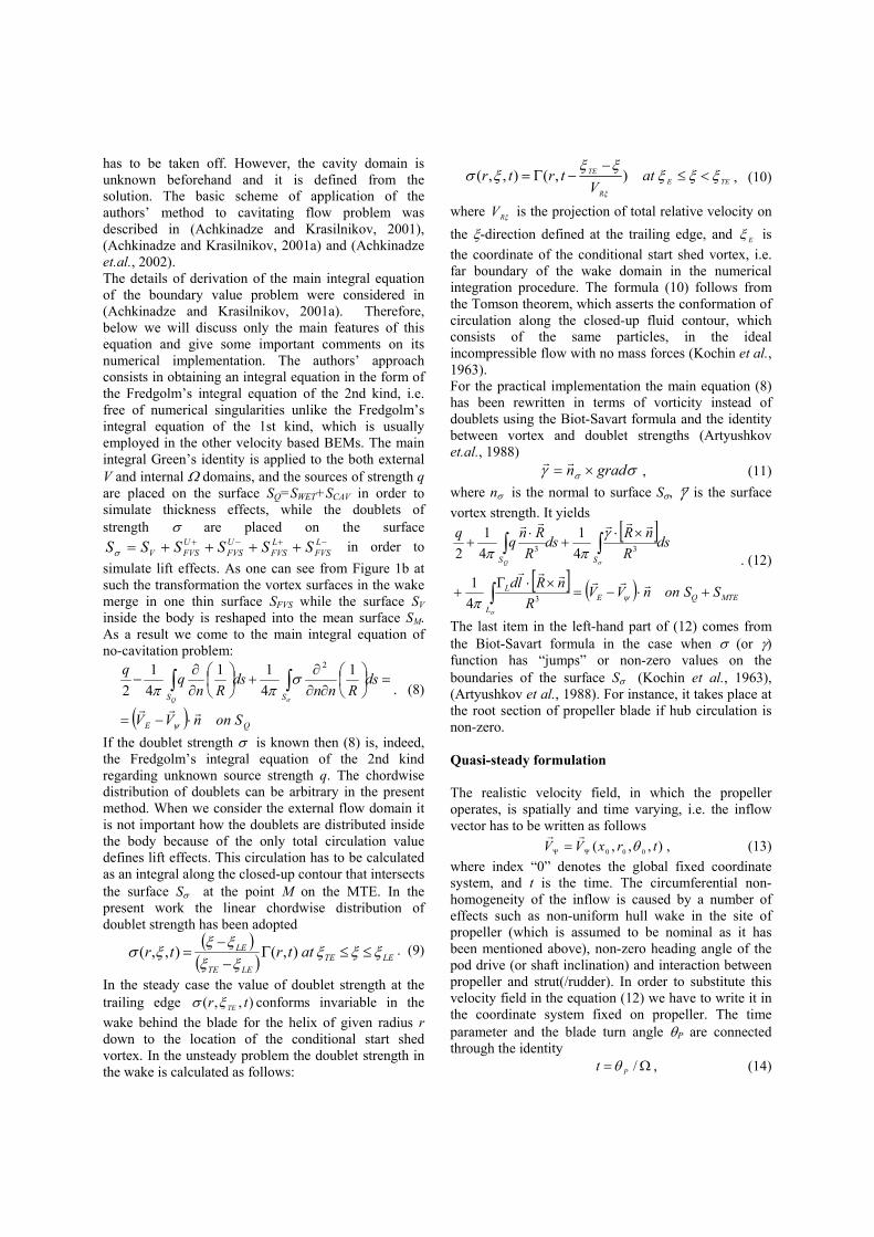
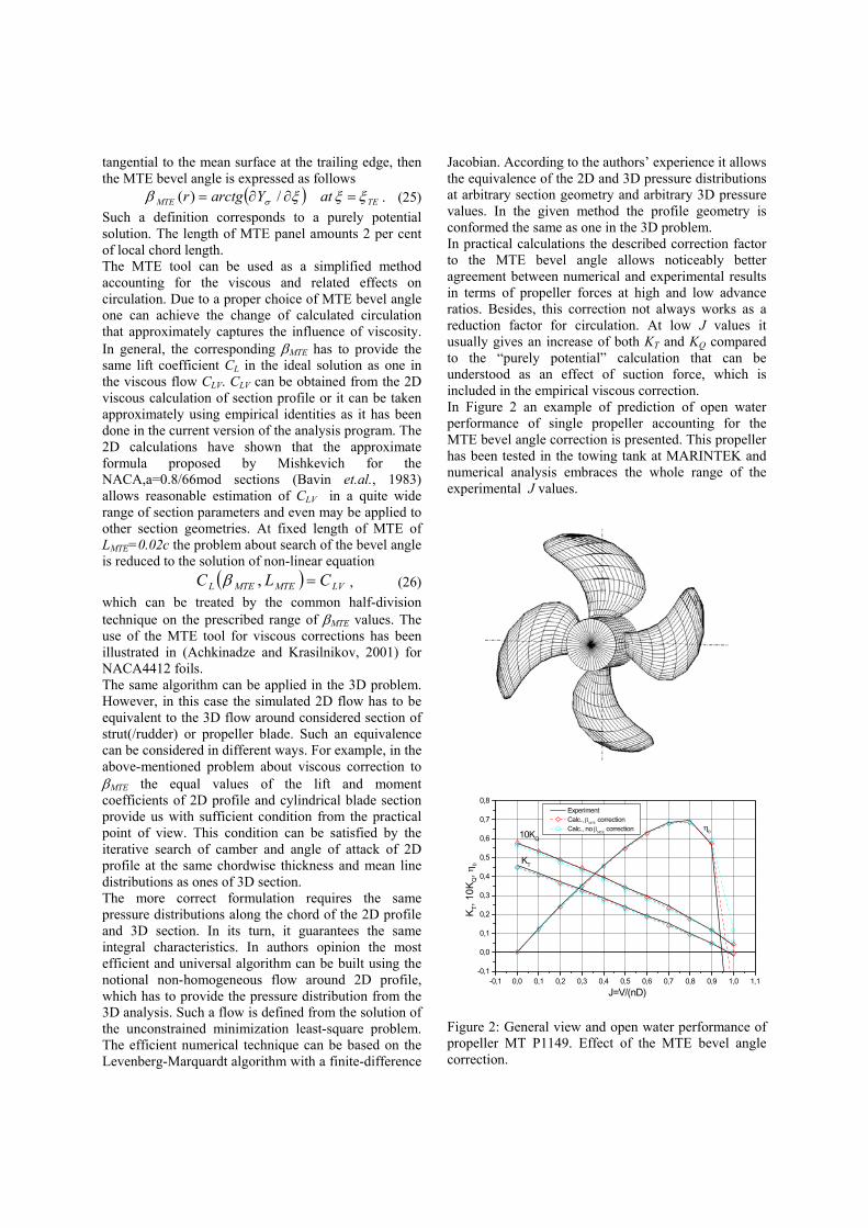
Jacobian. According to the authors’ experience it allows the equivalence of the 2D and 3D pressure distributions at arbitrary section geometry and arbitrary 3D pressure values. In the given method the profile geometry is conformed the same as one in the 3D problem. In practical calculations the described correction factor to the MTE bevel angle allows noticeably better agreement between numerical and experimental results in terms of propeller forces at high and low advance ratios. Besides, this correction not always works as a reduction factor for circulation. At low J values it usually gives an increase of both KT and KQ compared to the “purely potential” calculation that can be understood as an effect of suction force, which is included in the empirical viscous correction. In Figure 2 an example of prediction of open water performance of single propeller accounting for the MTE bevel angle correction is presented. This propeller has been tested in the towing tank at MARINTEK and numerical analysis embraces the whole range of the experimental J values.

-0,1 0,0 0,1 0,2 0,3 0,4 0,5 0,6 0,7 0,8 0,9 1,0 1,1-0,1

0,0

0,1

0,2

0,3

0,4

0,5

0,6

0,7

0,8

η010KQ

KT

Experiment Calc., β

ΜΤΕ correction

Calc., no βΜΤΕ

correction

K T, 10

K Q, η

0

J=V/(nD)

Figure 2: General view and open water performance of propeller MT P1149. Effect of the MTE bevel angle correction.

Computation of propeller-induced velocity field If pod- and rudder-induced velocity fields are calculated relatively fast and the only numerical singularity in the vortex wake behind rudder can be easily overcome through the proper disposition of calculation points, then propeller-induced velocity field requires more attention and finer tools than direct integration along the vortex wake. The adopted hypothesis about penetrability of the bodies for the trailing vortices allows us to build quite efficient and robust procedure for computation of propeller-induced velocities using the generalized infinite-bladed propeller theory by Hough and Ordway (Hough and Ordway, 1965). Generally, within the frameworks of potential theory this is probably the only way of accurate computation of propeller-induced velocities in the wake when the other bodies are present there, except, of course, the solution of the Euler equations as it has been done in (Kinnas et.al., 2001). The general identity for the velocity induced by the vortex wake trailing behind the lifting lines located in the propeller plane can be written down through the strengths of the straightforward and ring vortex components as follows:

×

+

+×

=

∫ ∫

∑ ∫ ∫∞

=

∞

R

r

RFW

Z

i

R

r

SFWFW

H

H

dR

Rir

dxR

RirW

03

1 03

)(41

)(41

θγπ

γπ

θ

rr

rrr

, (27)

where the mentioned strengths are defined through the circulation:

rdrr

drdZrS

FW πγ

21)()( Γ

−= , (28)

FVS

RFW rtg

drrdrdZr

βπγ

21)()( Γ

−= , (29)

and FVSβ is the pitch angle of the free vortex surface at

the given radius. In order to obtain the angular dependent velocity components Hough and Ordway performed the Fourier analysis of induced velocity field defined by (27) and proposed the expressions for the complex Fourier coefficients through the analytical Legendre functions of the 2nd kind and half-integer order. However, in the case of mean velocity field we need only 0-harmonics from these general identities. Taking into account that only ring vortices contribute in the axial and radial velocity components we can write the following identities:

∫=R

r

RFWx

H

drrrxKrW ),,()(21

111γπ

, (30)

∫−=R

r

RFWr

H

drQrrr

W )()(2

11

21

21

21

1

ωγπ

, (31)

where 1K and 21Q are calculated analytically through the Legendre special functions. The mean tangential induced velocity is defined by the well-known formula (Artyushkov et.al., 1988):

1

1

2)(

rrZ

WπθΓ

= , (32)

which is valid everywhere inside the propeller vortex wake restricted by the boundaries of the jet and propeller plane. Obviously, the written identities do not take into account effect of the vortices distributed on the mean surface within the blade contour. This effect can be included in the computational scheme using the method analogous to the Pien’s method in the lifting-surface theory. However, practical experience has shown that mentioned effect is concentrated only in the close vicinity of the blade where the blade thickness-induced velocities dominate, and can be neglected. It is confirmed, for example, by the results of prediction of velocity field in the wake of propeller DTMB4119 published by the authors in (Achkinadze and Krasilnikov, 2001a) where considered section was located extremely close to the blade trailing edge. At the same time, both “lifting-surface” and thickness-induced velocities vanish rather fast with the distance from propeller as upstream as downstream. There are, at least, two important effects, which have to be taken into account when using the obtained identities. The first of them is related to the influence of viscosity. Viscous effects manifest in two ways – as a reduction of “ideal” circulation caused by the section drag and as friction forces in the boundary layer on the blade surface. In order to capture the first effect the circulation Γ is reduced by the reduction coefficient, which is obtained from the comparison of propeller torque coefficient calculated with and without accounting for the section profile drag:

=Γ=Γ

Γ

Γ

QVQV

VV

KKCCrr

//)()(

. (33)

The friction in the boundary layer on the blade surface results in decrease of the axial velocity component in the wake and in increase of the swirl. In the present method the change of the axial component is taken as proportional to the displacement thickness δ* of boundary layer at given blade section, which is defined from the empirical identities. Then, the correction factors for the axial and tangential velocities in the wake can be derived from the condition of equal flowrates for the streamtube of radius r calculated with and without accounting for velocity correction factor:

( )( )( ) FVS

visx Rr

RbbZWβπ

δsin/

*−=∆ , (34)

FVSvis

xvis tgWW βθ /∆−=∆ . (35)

The second effect is related to contraction of propeller slipstream and, as the measurements show, it can be significant at high propeller loading. In the described procedure the simplest assumption about “linear” wake deformation has been adopted. Let us note that it does not imply modeling of propeller slipstream as a jet with straightforward bounds contracted at certain angle, but it is used only for definition of the velocity corrections at the given wake section. For each section this wake contraction parameter can be assigned separately, for instance, from the observations of propeller slipstream, and it is defined as a relation between the radii of deformed and non-deformed jets:

RRK WW /= . (36) Applying the momentum theorem to the contracted cylindrical jet we can obtain the following identities for the axial and tangential velocity components:

[ ]21)(1)(

41)( 2 −

++=

W

WxWxW

Cx K

rWrWrW , (37)

[ ][ ] 31

)(1)(

WC

x

WxW

C

KWrWW

rW++

= θθ , (38)

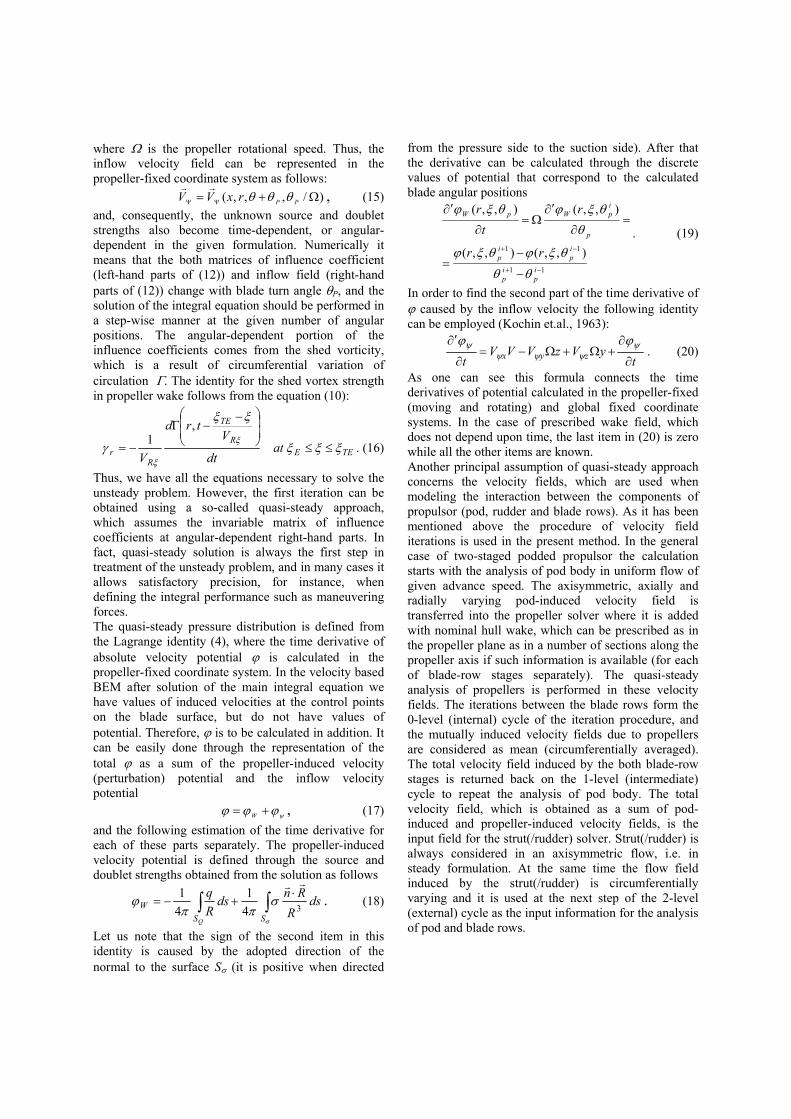
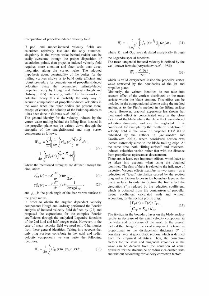
where WW Krr /= is the radius in the contracted jet that corresponds to the considered radius in the non-deformed jet. Numerical verification of propeller-induced velocity field algorithm was an important part of development of the analysis program for pod propulsors. Some results of this validation study have been published earlier, for example, in (Achkinadze and Krasilnikov, 2001a) where the comparison with LDV measurements in the wake of propeller DTMB4119 is given. However, as it has been mentioned above this case meets the wake section located extremely close to the blade trailing edge. Some calculations at more distant wake sections have been done in this work and the results have been compared with the LDV data borrowed from (Blaurock and Lammers, 1988). Figure 3 shows the comparison between calculated and measured axial and tangential velocities in the section x/R=−0.6 while the analogous data for the section x/R=−2.0 are given in Figure 4. In these calculations all the corrections – reduction of circulation, friction and wake contraction – have been used. The wake contraction coefficient amounted KW=0.92.

0.2 0.4 0.6 0.8 1.0 1.2

-0.1

0.0

0.1

0.2

0.3

0.4

0.5

0.6

0.7 LDV data calculation

axia

l vel

ocity

, -W

x/V

radius, r/R

0.2 0.4 0.6 0.8 1.0 1.2

0.0

0.1

0.2

0.3

0.4

0.5

0.6

LDV data calculation

tang

entia

l vel

ocity

, Wθ/

V

radius, r/R

Figure 3: Comparison between calculated and measured velocity components in the wake behind propeller BL2122. J=0.6. CTh=1.30. Wake section x/R=−0.6 Strut(/rudder) in propeller wake The analysis of strut(/rudder) is based on the same BEM approach as the propeller algorithm and its numerical implementation is similar to the latter in many respects. Discretization of rudder surface is performed in the same way as discretization of propeller blade using the cosine-type grid of curvilinear boundary elements. The zero values of circulation are required at the rudder tips and it defines the class of functions, which are employed for the approximation of spanwise loading distribution. It has to be noted that finer grid in the spanwise direction helps to get higher accuracy in definition of Γ when considering rudder in propeller wake. In this case the behaviour of circulation is quite complicated because of the flow swirl effect, especially when some parts of the rudder surface appear to be outside propeller jet.

0.0 0.2 0.4 0.6 0.8 1.0 1.2

-0.10.00.10.20.30.40.50.60.70.8

LDV data calculation

axia

l vel

ocity

, -W

x/V

radius, r/R

0.0 0.2 0.4 0.6 0.8 1.0 1.2

0.0

0.1

0.2

0.3

0.4

0.5

0.6 LDV data calculation

tang

entia

l vel

ocity

, Wθ/

V

radius, r/R

Figure 4: Comparison between calculated and measured velocity components in the wake behind propeller BL2122. J=0.6. CTh=1.30. Wake section x/R=−2.0 As it has been mentioned above the strut(/rudder) is considered in circumferentially averaged flow. A proper prediction of rudder surface pressure from the Bernoulli identity requires accounting for the “jump” of the Bernoulli constant that takes place in the propeller disk. The test calculations have shown that the direct use of the Bernoulli identity without any corrections yields the pressure distribution as though moved regarding the experimental distribution. The mentioned correction factor has to provide the absence of propeller-induced pressure at the wake section located “very far” downstream the propeller. It meets the known experimental fact obtained for the open propellers, which consists in the equality of pressure values in the undisturbed flow in front of propeller and in the far propeller wake. The experiments show the decrease of the time-averaged pressure measured along the streamline in front of propeller, then extremely fast increase (“jump”) in the site of propeller and then again smooth decrease in propeller wake down to the values in undisturbed flow. The simplified method accounting for this effect adopted in the present work consists in

estimation of the change of the Bernoulli constant at one radius that corresponds to the maximum axial propeller-induced velocity. Although, strictly, the correction factor should be calculated for each streamline passing through the propeller disk, the applied estimation guarantees the maximum possible value of the mentioned pressure “jump”. Then, the corrected pressure value on the rudder surface can be calculated as follows:

∞∆−= CpCpCp* , 2)(1 ER VVCp ∞∞ −=∆ , (39)

where PC is the pressure coefficient defined from the

Bernoulli identity without correction, ∞RV is the total

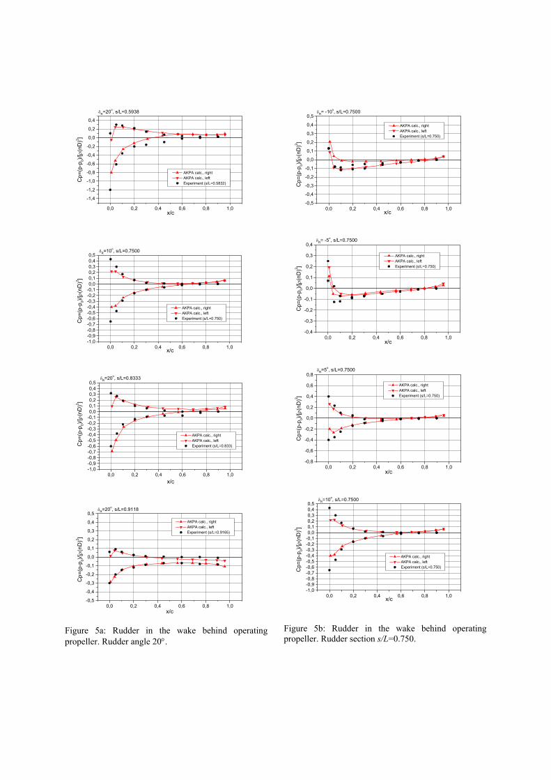
relative velocity estimated in the far wake behind the propeller at the radius of maximum axial propeller-induced velocity. The similar correction is applied when calculating the blade pressure on the aft blade row of two-stage system. The numerical/experimental verification of propeller/rudder analysis program has been performed using the pressure measurements on the rudder surface available from (Tamashima and Yamazaki, 1992). The main data on propeller/rudder arrangement are summarized in Table 1. Figure 5a presents the authors’ results obtained at rudder angle of 20° in the different span locations while Figure 5b shows the pressure distributions along the section s/L=0.75 (75 per cent from the rudder lower tip) at different rudder angles. The pressure correction factor according to (39) has been used in these calculations for the rudder sections immersed in the propeller wake. It is not necessary to include any corrections for the sections outside the propeller wake. A satisfactory agreement between calculations and measurements has been achieved. Table 1: Main elements of propeller/rudder arrangement used in the comparison with experiment from (Tamashima and Yamazaki, 1992):

Rudder span/Prop diameter L/D=1.256

Number of prop blades Z=5

Rudder aspect ratio L/c=1.5

Distance between prop plane and rudder axis XR/D=0.54

Vertical position of rudder regarding prop axis Symm.

Propeller thrust loading coefficient CTh=2.32

0,0 0,2 0,4 0,6 0,8 1,0

-1,4

-1,2

-1,0

-0,8

-0,6

-0,4

-0,2

0,0

0,2

0,4

δR=20o, s/L=0.5938

AKPA calc., right AKPA calc., left Experiment (s/L=0.5832)C

p=(p

-p0)/

[ρ(n

D)2 ]

x/c

0,0 0,2 0,4 0,6 0,8 1,0-1,0-0,9-0,8-0,7-0,6-0,5-0,4-0,3-0,2-0,10,00,10,20,30,40,5

δR=10o, s/L=0.7500


p=(p

-p0)/

[ρ(n

D)2 ]

x/c

0,0 0,2 0,4 0,6 0,8 1,0-1,0-0,9-0,8-0,7-0,6-0,5-0,4-0,3-0,2-0,10,00,10,20,30,40,5

δR=20o, s/L=0.8333


p=(p

-p0)/

[ρ(n

D)2 ]

x/c

0,0 0,2 0,4 0,6 0,8 1,0-0,5

-0,4

-0,3

-0,2

-0,1

0,0

0,1

0,2

0,3

0,4

0,5δR=20o, s/L=0.9118

AKPA calc., right AKPA calc., left Experiment (s/L=0.9165)

Cp=

(p-p

0)/[ρ

(nD

)2 ]

x/c

Figure 5a: Rudder in the wake behind operating propeller. Rudder angle 20°.

0,0 0,2 0,4 0,6 0,8 1,0-0,5

-0,4

-0,3

-0,2

-0,1

0,0

0,1

0,2

0,3

0,4

0,5δR= -10o, s/L=0.7500


Cp=

(p-p

0)/[ρ

(nD

)2 ]

x/c

0,0 0,2 0,4 0,6 0,8 1,0-0,4

-0,3

-0,2

-0,1

0,0

0,1

0,2

0,3

0,4δR= -5o, s/L=0.7500


Cp=

(p-p

0)/[ρ

(nD

)2 ]

x/c

0,0 0,2 0,4 0,6 0,8 1,0-0,8

-0,6

-0,4

-0,2

0,0

0,2

0,4

0,6

0,8δR=5o, s/L=0.7500


Cp=

(p-p

0)/[ρ

(nD

)2 ]

x/c

0,0 0,2 0,4 0,6 0,8 1,0-1,0-0,9-0,8-0,7-0,6-0,5-0,4-0,3-0,2-0,10,00,10,20,30,40,5

δR=10o, s/L=0.7500


p=(p

-p0)/

[ρ(n

D)2 ]

x/c

Figure 5b: Rudder in the wake behind operating propeller. Rudder section s/L=0.750.

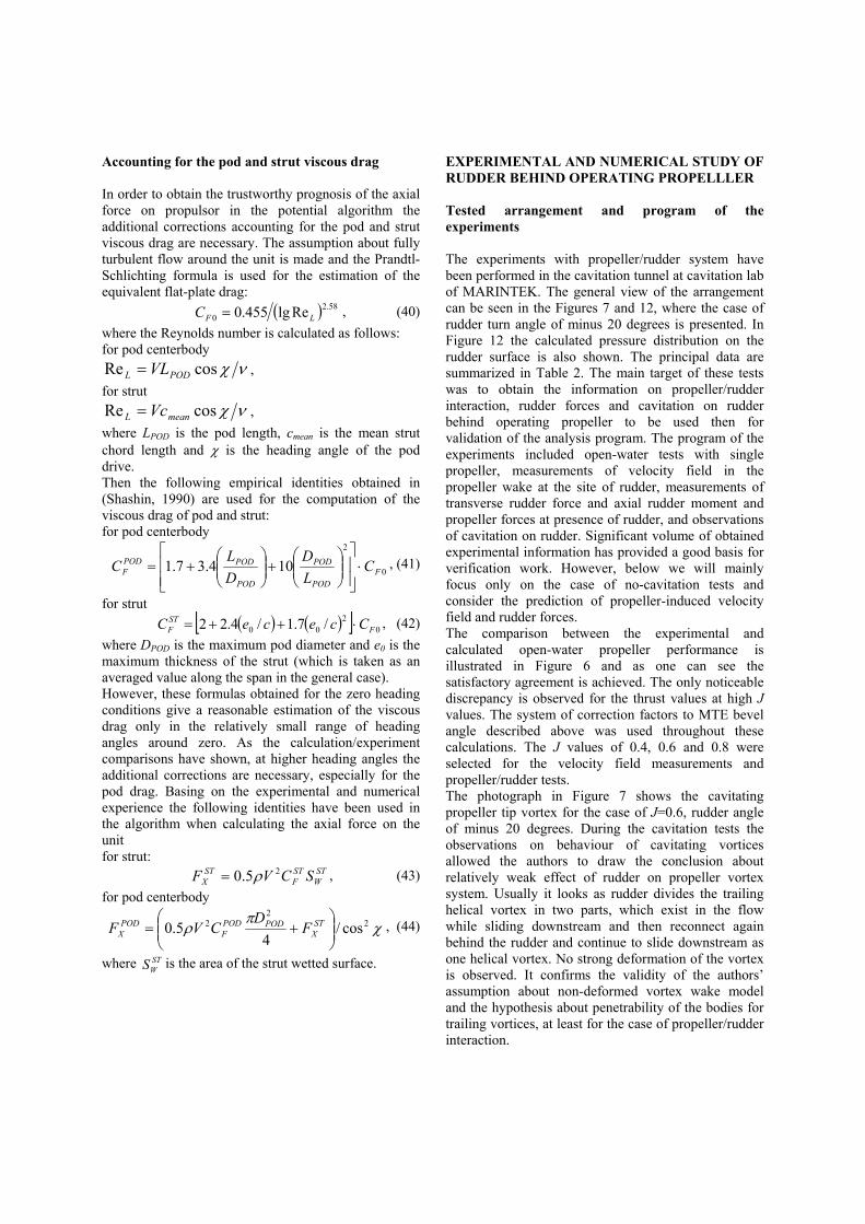
Accounting for the pod and strut viscous drag In order to obtain the trustworthy prognosis of the axial force on propulsor in the potential algorithm the additional corrections accounting for the pod and strut viscous drag are necessary. The assumption about fully turbulent flow around the unit is made and the Prandtl-Schlichting formula is used for the estimation of the equivalent flat-plate drag:

( ) 58.20 Relg455.0 LFC = , (40)

where the Reynolds number is calculated as follows: for pod centerbody

νχcosRe PODL VL= , for strut

νχcosRe meanL Vc= , where LPOD is the pod length, cmean is the mean strut chord length and χ is the heading angle of the pod drive. Then the following empirical identities obtained in (Shashin, 1990) are used for the computation of the viscous drag of pod and strut: for pod centerbody

0

2

104.37.1 FPOD

POD

POD

PODPODF C

LD

DL

C ⋅

+

+= , (41)

for strut ( ) ( )[ ] 0

200 /7.1/4.22 F

STF CceceC ⋅++= , (42)

where DPOD is the maximum pod diameter and e0 is the maximum thickness of the strut (which is taken as an averaged value along the span in the general case). However, these formulas obtained for the zero heading conditions give a reasonable estimation of the viscous drag only in the relatively small range of heading angles around zero. As the calculation/experiment comparisons have shown, at higher heading angles the additional corrections are necessary, especially for the pod drag. Basing on the experimental and numerical experience the following identities have been used in the algorithm when calculating the axial force on the unit for strut:

STW

STF

STX SCVF 25.0 ρ= , (43)

for pod centerbody

χπ

ρ 22

2 cos/4

5.0

+= ST

XPODPOD

FPOD

X FD

CVF , (44)

where STWS is the area of the strut wetted surface.

EXPERIMENTAL AND NUMERICAL STUDY OF RUDDER BEHIND OPERATING PROPELLLER Tested arrangement and program of the experiments The experiments with propeller/rudder system have been performed in the cavitation tunnel at cavitation lab of MARINTEK. The general view of the arrangement can be seen in the Figures 7 and 12, where the case of rudder turn angle of minus 20 degrees is presented. In Figure 12 the calculated pressure distribution on the rudder surface is also shown. The principal data are summarized in Table 2. The main target of these tests was to obtain the information on propeller/rudder interaction, rudder forces and cavitation on rudder behind operating propeller to be used then for validation of the analysis program. The program of the experiments included open-water tests with single propeller, measurements of velocity field in the propeller wake at the site of rudder, measurements of transverse rudder force and axial rudder moment and propeller forces at presence of rudder, and observations of cavitation on rudder. Significant volume of obtained experimental information has provided a good basis for verification work. However, below we will mainly focus only on the case of no-cavitation tests and consider the prediction of propeller-induced velocity field and rudder forces. The comparison between the experimental and calculated open-water propeller performance is illustrated in Figure 6 and as one can see the satisfactory agreement is achieved. The only noticeable discrepancy is observed for the thrust values at high J values. The system of correction factors to MTE bevel angle described above was used throughout these calculations. The J values of 0.4, 0.6 and 0.8 were selected for the velocity field measurements and propeller/rudder tests. The photograph in Figure 7 shows the cavitating propeller tip vortex for the case of J=0.6, rudder angle of minus 20 degrees. During the cavitation tests the observations on behaviour of cavitating vortices allowed the authors to draw the conclusion about relatively weak effect of rudder on propeller vortex system. Usually it looks as rudder divides the trailing helical vortex in two parts, which exist in the flow while sliding downstream and then reconnect again behind the rudder and continue to slide downstream as one helical vortex. No strong deformation of the vortex is observed. It confirms the validity of the authors’ assumption about non-deformed vortex wake model and the hypothesis about penetrability of the bodies for trailing vortices, at least for the case of propeller/rudder interaction.

0,1 0,2 0,3 0,4 0,5 0,6 0,7 0,8 0,9 1,0 1,1 1,2 1,30,0

0,1

0,2

0,3

0,4

0,5

0,6

0,7

0,8

10KQ

KT

Experiment Calculation

K T, 10

K Q

Advance ratio, J=V/(nD)

Figure 6: Experimental and calculated open-water thrust and torque coefficients of propeller used in the propeller/rudder tests.

Figure 7: Interaction of cavitating propeller tip vortex with rudder. J=0.6. Rudder angle δR=−20°.

Table 2: Main elements of propeller/rudder arrangement used in the experimental/numerical study at MARINTEK:

Prop diameter D=0.25m

Number of prop blades Z=4

Blade area ratio 0.61

Pitch ratio at r/R=0.7 P/D=1.095

Rudder span/Prop diameter L/D=1.251

Rudder aspect ratio L/c=1.916

Distance between prop plane and rudder axis XR/D=0.5

Location of rudder axis, % from rudder LE 28.8

Vertical position of rudder regarding prop axis Asymm.

Test conditions, J=0.8, 0.6, 0.4

Rudder angles, δR∈[−30°;+30°]

0,1 0,2 0,3 0,4 0,5 0,6 0,7 0,8 0,9 1,0 1,1 1,2-0,1

0,0

0,1

0,2

0,3

0,4

0,5J=0.8, x/R=-1.00

Experiment Calc, Kw=0.96ax

ial v

eloc

ity, -

Wx/

V

r/R

0,1 0,2 0,3 0,4 0,5 0,6 0,7 0,8 0,9 1,0 1,1 1,2-0,05

0,00

0,05

0,10

0,15

0,20

0,25

0,30J=0.8, x/R=-1.00

Exp Calc, Kw=0.96

tang

entia

l vel

ocity

, Wθ/V

r/R

Figure 8: Comparison between measured and calculated propeller-induced velocity components in the wake behind propeller. J=0.8. CTh=0.754. Section x/R=−1.0. Wake contraction factor KW=0.96.

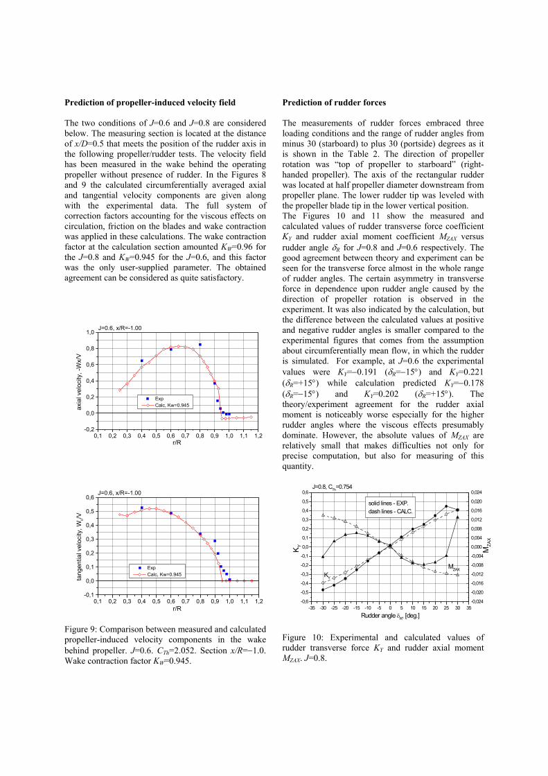
Prediction of propeller-induced velocity field The two conditions of J=0.6 and J=0.8 are considered below. The measuring section is located at the distance of x/D=0.5 that meets the position of the rudder axis in the following propeller/rudder tests. The velocity field has been measured in the wake behind the operating propeller without presence of rudder. In the Figures 8 and 9 the calculated circumferentially averaged axial and tangential velocity components are given along with the experimental data. The full system of correction factors accounting for the viscous effects on circulation, friction on the blades and wake contraction was applied in these calculations. The wake contraction factor at the calculation section amounted KW=0.96 for the J=0.8 and KW=0.945 for the J=0.6, and this factor was the only user-supplied parameter. The obtained agreement can be considered as quite satisfactory.

0,1 0,2 0,3 0,4 0,5 0,6 0,7 0,8 0,9 1,0 1,1 1,2-0,2

0,0

0,2

0,4

0,6

0,8

1,0J=0.6, x/R=-1.00

Exp Calc, Kw=0.945ax

ial v

eloc

ity, -

Wx/

V

r/R

0,1 0,2 0,3 0,4 0,5 0,6 0,7 0,8 0,9 1,0 1,1 1,2-0,1

0,0

0,1

0,2

0,3

0,4

0,5

0,6J=0.6, x/R=-1.00

Exp Calc, Kw=0.945

tang

entia

l vel

ocity

, Wθ/V

r/R

Figure 9: Comparison between measured and calculated propeller-induced velocity components in the wake behind propeller. J=0.6. CTh=2.052. Section x/R=−1.0. Wake contraction factor KW=0.945.

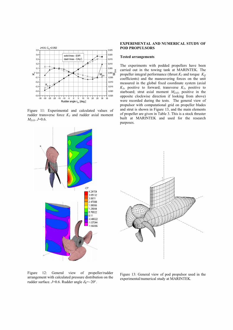
Prediction of rudder forces The measurements of rudder forces embraced three loading conditions and the range of rudder angles from minus 30 (starboard) to plus 30 (portside) degrees as it is shown in the Table 2. The direction of propeller rotation was “top of propeller to starboard” (right-handed propeller). The axis of the rectangular rudder was located at half propeller diameter downstream from propeller plane. The lower rudder tip was leveled with the propeller blade tip in the lower vertical position. The Figures 10 and 11 show the measured and calculated values of rudder transverse force coefficient KY and rudder axial moment coefficient MZAX versus rudder angle δR for J=0.8 and J=0.6 respectively. The good agreement between theory and experiment can be seen for the transverse force almost in the whole range of rudder angles. The certain asymmetry in transverse force in dependence upon rudder angle caused by the direction of propeller rotation is observed in the experiment. It was also indicated by the calculation, but the difference between the calculated values at positive and negative rudder angles is smaller compared to the experimental figures that comes from the assumption about circumferentially mean flow, in which the rudder is simulated. For example, at J=0.6 the experimental values were KY=−0.191 (δR=−15°) and KY=0.221 (δR=+15°) while calculation predicted KY=−0.178 (δR=−15°) and KY=0.202 (δR=+15°). The theory/experiment agreement for the rudder axial moment is noticeably worse especially for the higher rudder angles where the viscous effects presumably dominate. However, the absolute values of MZAX are relatively small that makes difficulties not only for precise computation, but also for measuring of this quantity.

-35 -30 -25 -20 -15 -10 -5 0 5 10 15 20 25 30 35-0,6

-0,5

-0,4

-0,3

-0,2

-0,1

0,0

0,1

0,2

0,3

0,4

0,5

0,6

solid lines - EXP.dash lines - CALC.

MZA

X

K Y

Rudder angle δR, [deg.]

-0,024

-0,020

-0,016

-0,012

-0,008

-0,004

0,000

0,004

0,008

0,012

0,016

0,020

0,024J=0.8, CTh=0.754

MZAXKY

Figure 10: Experimental and calculated values of rudder transverse force KY and rudder axial moment MZAX. J=0.8.

-35 -30 -25 -20 -15 -10 -5 0 5 10 15 20 25 30 35-0,5

-0,4

-0,3

-0,2

-0,1

0,0

0,1

0,2

0,3

0,4

0,5J=0.6, CTh=2.052


MZAX

KY

MZA

X

K Y

Rudder angle δR, [deg.]

-0,025

-0,020

-0,015

-0,010

-0,005

0,000

0,005

0,010

0,015

0,020

0,025

Figure 11: Experimental and calculated values of rudder transverse force KY and rudder axial moment MZAX. J=0.6. Figure 12: General view of propeller/rudder arrangement with calculated pressure distribution on the rudder surface. J=0.6. Rudder angle δR=−20°.

EXPERIMENTAL AND NUMERICAL STUDY OF POD PROPULSORS Tested arrangements The experiments with podded propellers have been carried out in the towing tank at MARINTEK. The propeller integral performance (thrust KT and torque KQ coefficients) and the maneuvering forces on the unit measured in the global fixed coordinate system (axial KX, positive to forward; transverse KY, positive to starboard; strut axial moment MZAX, positive in the opposite clockwise direction if looking from above) were recorded during the tests. The general view of propulsor with computational grid on propeller blades and strut is shown in Figure 13, and the main elements of propeller are given in Table 3. This is a stock thruster built at MARINTEK and used for the research purposes.

Figure 13: General view of pod propulsor used in the experimental/numerical study at MARINTEK.

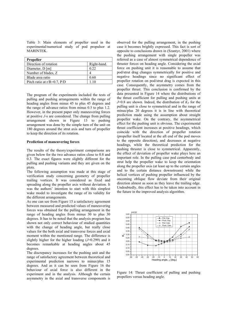
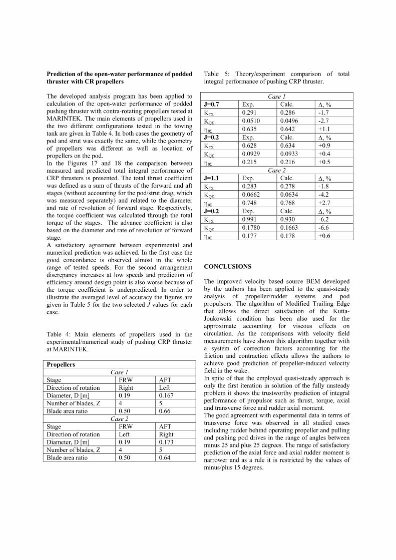
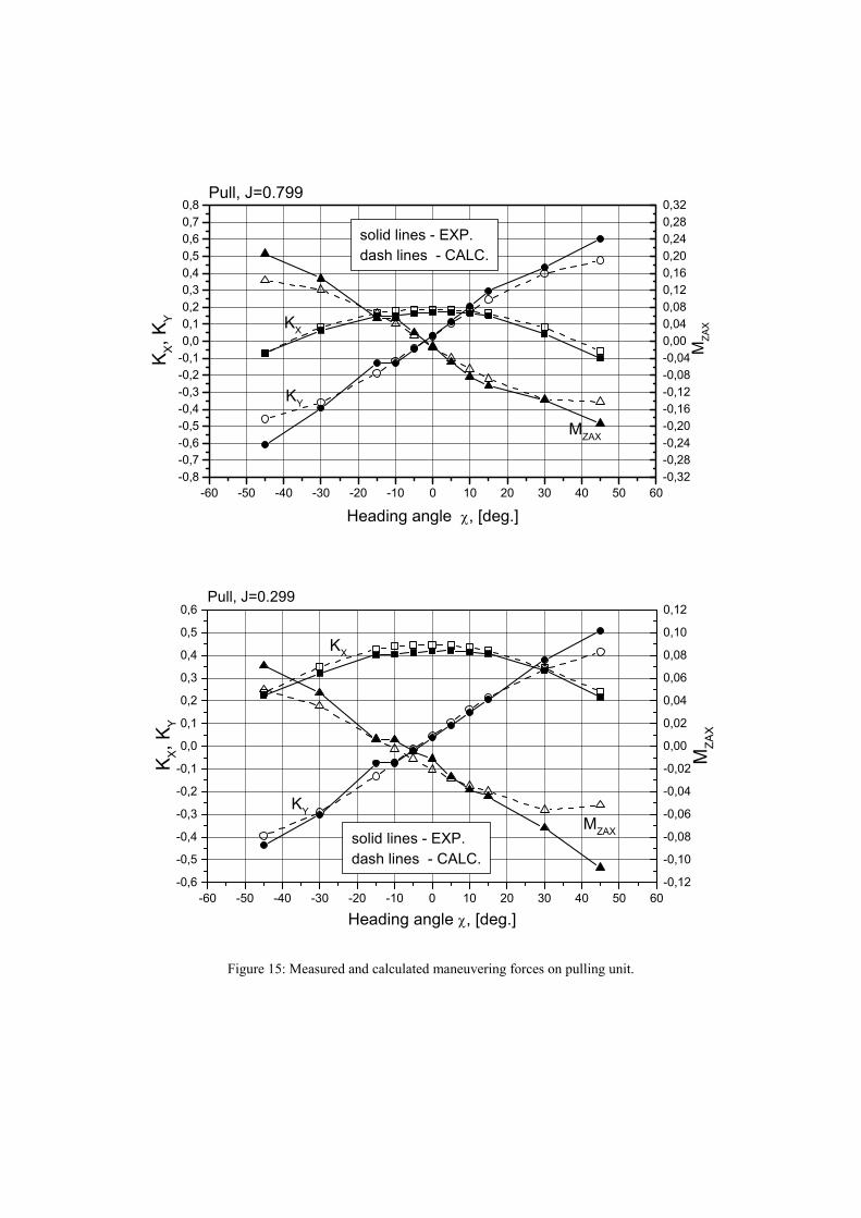
Table 3: Main elements of propeller used in the experimental/numerical study of pod propulsor at MARINTEK. Propeller Direction of rotation Right-hand. Diameter, D [m] 0.22 Number of blades, Z 4 Blade area ratio 0.60 Pitch ratio at r/R=0.7, P/D 1.10 The program of the experiments included the tests of pulling and pushing arrangements within the range of heading angles from minus 45 to plus 45 degrees and the range of advance ratios from minus 0.5 to plus 1.2. However, in the present paper only maneuvering forces at positive J-s are considered. The change from pulling arrangement shown in Figure 13 to pushing arrangement was done by the simple turn of the unit on 180 degrees around the strut axis and turn of propeller to keep the direction of its rotation. Prediction of maneuvering forces The results of the theory/experiment comparisons are given below for the two advance ratios close to 0.8 and 0.3. The exact figures were slightly different for the pulling and pushing variants and they are given on the plots. The following assumption was made at this stage of verification study concerning geometry of propeller trailing vortices. It was considered as fixed and spreading along the propeller axis without deviation. It was the authors’ intention to start with this simplest wake model to investigate the range of its validity for the different arrangements. As one can see from Figure 15 a satisfactory agreement between measured and predicted values of maneuvering forces was obtained for the pulling arrangement in the range of heading angles from minus 30 to plus 30 degrees. It has to be noted that the analysis program has shown not only correct behaviour of studied quantities with the change of heading angle, but really close values for the both axial and transverse forces and axial moment within the mentioned range. The difference is slightly higher for the higher loading (J=0.299) and it becomes remarkable at heading angles about 45 degrees. The discrepancy increases for the pushing unit and the range of satisfactory agreement between theoretical and experimental prediction narrows to minus/plus 15 degrees. And as it can be seen from Figure 16 the behaviour of axial force is also different in the experiment and in the analysis. Although the certain asymmetry in the axial and transverse components is

observed for the pulling arrangement, in the pushing case it becomes brightly expressed. This fact is sort of opposite to conclusions drawn in (Szantyr, 2001) where the pushing arrangement with single propeller was referred as a case of almost symmetrical dependence of thruster forces on heading angle. Considering the axial force on pushing unit it is reasonable to assume that pod/strut drag changes symmetrically for positive and negative headings since no significant effect of propeller rotation on pod/strut drag is expected in this case. Consequently, the asymmetry comes from the propeller thrust. This conclusion is confirmed by the data presented in Figure 14 where the distributions of the thrust coefficient for pulling and pushing units at J=0.8 are shown. Indeed, the distribution of KT for the pulling unit is close to symmetrical and in the range of minus/plus 20 degrees it is in line with theoretical prediction made using the assumption about straight propeller wake. On the contrary, the asymmetrical effect for the pushing unit is obvious. The experimental thrust coefficient increases at positive headings, which coincide with the direction of propeller rotation (propeller itself located at the aft end of the pod moves to the opposite direction), and decreases at negative headings, while the theoretical prediction for the pushing thruster is close to symmetrical. Apparently, the effect of deviation of propeller wake plays here an important role. In the pulling case pod centerbody and strut help the propeller wake to keep the orientation along the propeller axis (at least up to the certain angles and to the certain distance downstream) while the helical vortices of pushing propeller influenced by the oncoming oblique flow deviate from their original direction almost as soon as they leave the trailing edge. Undoubtedly, this effect has to be taken into account in the future in the improved analysis algorithm.

-60 -50 -40 -30 -20 -10 0 10 20 30 40 50 600,00

0,05

0,10

0,15

0,20

0,25

0,30

0,35

0,40

0,45

0,50

0,55

0,60J=0.8

Pull, Exp. Push, Exp. Pull, Calc. Push, Calc.

K T

Heading angle, χ [deg.]

Figure 14: Thrust coefficient of pulling and pushing propellers versus heading angle.

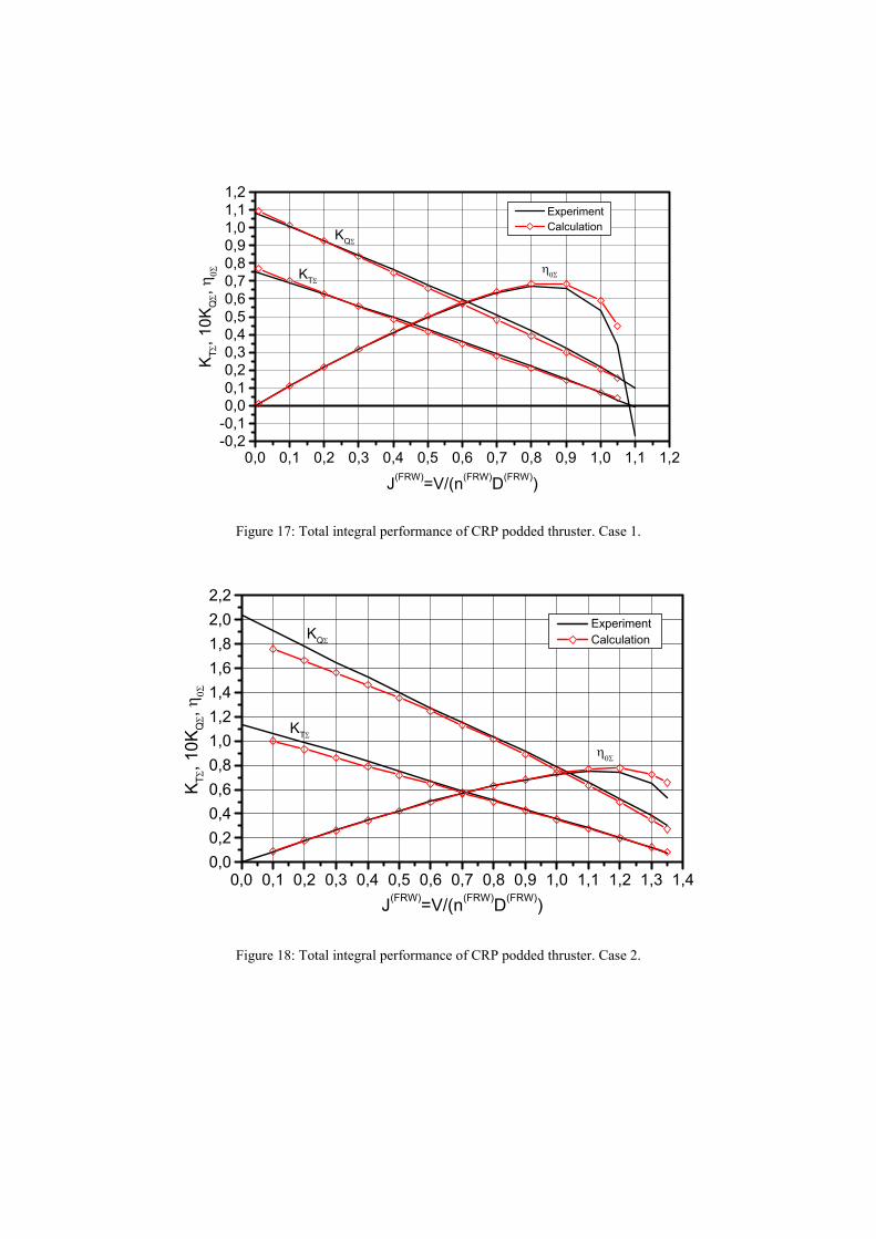
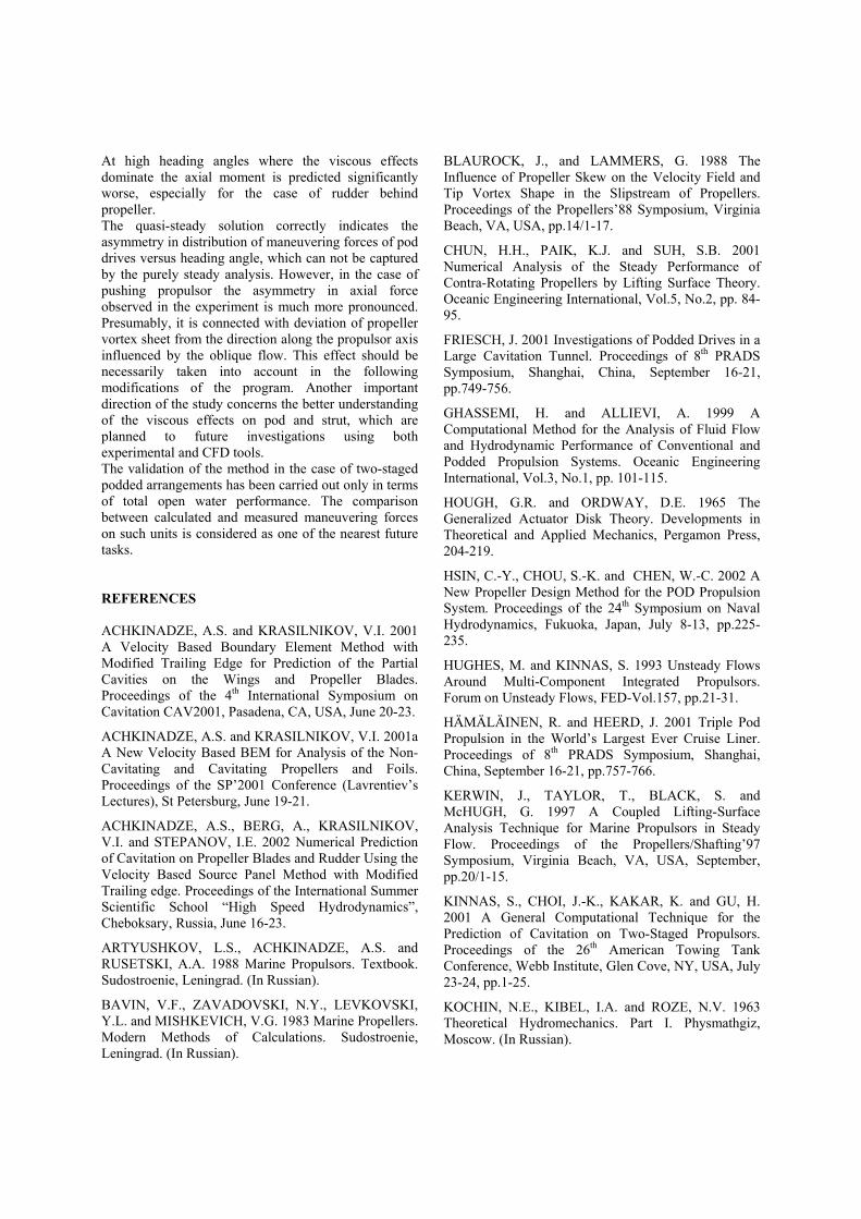
Prediction of the open-water performance of podded thruster with CR propellers The developed analysis program has been applied to calculation of the open-water performance of podded pushing thruster with contra-rotating propellers tested at MARINTEK. The main elements of propellers used in the two different configurations tested in the towing tank are given in Table 4. In both cases the geometry of pod and strut was exactly the same, while the geometry of propellers was different as well as location of propellers on the pod. In the Figures 17 and 18 the comparison between measured and predicted total integral performance of CRP thrusters is presented. The total thrust coefficient was defined as a sum of thrusts of the forward and aft stages (without accounting for the pod/strut drag, which was measured separately) and related to the diameter and rate of revolution of forward stage. Respectively, the torque coefficient was calculated through the total torque of the stages. The advance coefficient is also based on the diameter and rate of revolution of forward stage. A satisfactory agreement between experimental and numerical prediction was achieved. In the first case the good concordance is observed almost in the whole range of tested speeds. For the second arrangement discrepancy increases at low speeds and prediction of efficiency around design point is also worse because of the torque coefficient is underpredicted. In order to illustrate the averaged level of accuracy the figures are given in Table 5 for the two selected J values for each case. Table 4: Main elements of propellers used in the experimental/numerical study of pushing CRP thruster at MARINTEK. Propellers

Case 1 Stage FRW AFT Direction of rotation Right Left Diameter, D [m] 0.19 0.167 Number of blades, Z 4 5 Blade area ratio 0.50 0.66

Case 2 Stage FRW AFT Direction of rotation Left Right Diameter, D [m] 0.19 0.173 Number of blades, Z 4 5 Blade area ratio 0.50 0.64

Table 5: Theory/experiment comparison of total integral performance of pushing CRP thruster.

Case 1 J=0.7 Exp. Calc. ∆, % KTΣ 0.291 0.286 -1.7 KQΣ 0.0510 0.0496 -2.7 η0Σ 0.635 0.642 +1.1 J=0.2 Exp. Calc. ∆, % KTΣ 0.628 0.634 +0.9 KQΣ 0.0929 0.0933 +0.4 η0Σ 0.215 0.216 +0.5

Case 2 J=1.1 Exp. Calc. ∆, % KTΣ 0.283 0.278 -1.8 KQΣ 0.0662 0.0634 -4.2 η0Σ 0.748 0.768 +2.7 J=0.2 Exp. Calc. ∆, % KTΣ 0.991 0.930 -6.2 KQΣ 0.1780 0.1663 -6.6 η0Σ 0.177 0.178 +0.6 CONCLUSIONS The improved velocity based source BEM developed by the authors has been applied to the quasi-steady analysis of propeller/rudder systems and pod propulsors. The algorithm of Modified Trailing Edge that allows the direct satisfaction of the Kutta-Joukowski condition has been also used for the approximate accounting for viscous effects on circulation. As the comparisons with velocity field measurements have shown this algorithm together with a system of correction factors accounting for the friction and contraction effects allows the authors to achieve good prediction of propeller-induced velocity field in the wake. In spite of that the employed quasi-steady approach is only the first iteration in solution of the fully unsteady problem it shows the trustworthy prediction of integral performance of propulsor such as thrust, torque, axial and transverse force and rudder axial moment. The good agreement with experimental data in terms of transverse force was observed in all studied cases including rudder behind operating propeller and pulling and pushing pod drives in the range of angles between minus 25 and plus 25 degrees. The range of satisfactory prediction of the axial force and axial rudder moment is narrower and as a rule it is restricted by the values of minus/plus 15 degrees.

-60 -50 -40 -30 -20 -10 0 10 20 30 40 50 60-0,8-0,7-0,6-0,5-0,4-0,3-0,2-0,10,00,10,20,30,40,50,60,70,8

Pull, J=0.799

MZAX

KX

KY

MZA

X

K X, K Y

Heading angle χ, [deg.]

-0,32-0,28-0,24-0,20-0,16-0,12-0,08-0,040,000,040,080,120,160,200,240,280,32


-60 -50 -40 -30 -20 -10 0 10 20 30 40 50 60-0,6

-0,5

-0,4

-0,3

-0,2

-0,1

0,0

0,1

0,2

0,3

0,4

0,5

0,6


MZAX

KX

KY

Pull, J=0.299

MZA

X

K X, K Y


-0,12

-0,10

-0,08

-0,06

-0,04

-0,02

0,00

0,02

0,04

0,06

0,08

0,10

0,12

Figure 15: Measured and calculated maneuvering forces on pulling unit.

-60 -50 -40 -30 -20 -10 0 10 20 30 40 50 60-0,8-0,7-0,6-0,5-0,4-0,3-0,2-0,10,00,10,20,30,40,50,60,70,8

Push, J=0.813


MZAX

KX

KY

MZA

X

K X, K Y


-0,16-0,14-0,12-0,10-0,08-0,06-0,04-0,020,000,020,040,060,080,100,120,140,16

-60 -50 -40 -30 -20 -10 0 10 20 30 40 50 60-0,6

-0,5

-0,4

-0,3

-0,2

-0,1

0,0

0,1

0,2

0,3

0,4

0,5

0,6Push, J=0.3088


MZAX

KX

KY

MZA

X

K X, K Y


-0,12

-0,10

-0,08

-0,06

-0,04

-0,02

0,00

0,02

0,04

0,06

0,08

0,10

0,12

Figure 16: Measured and calculated maneuvering forces on pushing unit.

0,0 0,1 0,2 0,3 0,4 0,5 0,6 0,7 0,8 0,9 1,0 1,1 1,2-0,2-0,10,00,10,20,30,40,50,60,70,80,91,01,11,2

η0Σ

KQΣ

KTΣ


K TΣ, 1

0KQΣ, η 0

Σ

J(FRW)=V/(n(FRW)D(FRW))

Figure 17: Total integral performance of CRP podded thruster. Case 1.

0,0 0,1 0,2 0,3 0,4 0,5 0,6 0,7 0,8 0,9 1,0 1,1 1,2 1,3 1,40,00,20,40,60,81,01,21,41,61,82,02,2

η0Σ

KQΣ

KTΣ


K TΣ, 1

0KQΣ, η 0

Σ

J(FRW)=V/(n(FRW)D(FRW))

Figure 18: Total integral performance of CRP podded thruster. Case 2.

At high heading angles where the viscous effects dominate the axial moment is predicted significantly worse, especially for the case of rudder behind propeller. The quasi-steady solution correctly indicates the asymmetry in distribution of maneuvering forces of pod drives versus heading angle, which can not be captured by the purely steady analysis. However, in the case of pushing propulsor the asymmetry in axial force observed in the experiment is much more pronounced. Presumably, it is connected with deviation of propeller vortex sheet from the direction along the propulsor axis influenced by the oblique flow. This effect should be necessarily taken into account in the following modifications of the program. Another important direction of the study concerns the better understanding of the viscous effects on pod and strut, which are planned to future investigations using both experimental and CFD tools. The validation of the method in the case of two-staged podded arrangements has been carried out only in terms of total open water performance. The comparison between calculated and measured maneuvering forces on such units is considered as one of the nearest future tasks. REFERENCES ACHKINADZE, A.S. and KRASILNIKOV, V.I. 2001 A Velocity Based Boundary Element Method with Modified Trailing Edge for Prediction of the Partial Cavities on the Wings and Propeller Blades. Proceedings of the 4th International Symposium on Cavitation CAV2001, Pasadena, CA, USA, June 20-23.

ACHKINADZE, A.S. and KRASILNIKOV, V.I. 2001a A New Velocity Based BEM for Analysis of the Non-Cavitating and Cavitating Propellers and Foils. Proceedings of the SP’2001 Conference (Lavrentiev’s Lectures), St Petersburg, June 19-21.

ACHKINADZE, A.S., BERG, A., KRASILNIKOV, V.I. and STEPANOV, I.E. 2002 Numerical Prediction of Cavitation on Propeller Blades and Rudder Using the Velocity Based Source Panel Method with Modified Trailing edge. Proceedings of the International Summer Scientific School “High Speed Hydrodynamics”, Cheboksary, Russia, June 16-23.

ARTYUSHKOV, L.S., ACHKINADZE, A.S. and RUSETSKI, A.A. 1988 Marine Propulsors. Textbook. Sudostroenie, Leningrad. (In Russian).

BAVIN, V.F., ZAVADOVSKI, N.Y., LEVKOVSKI, Y.L. and MISHKEVICH, V.G. 1983 Marine Propellers. Modern Methods of Calculations. Sudostroenie, Leningrad. (In Russian).

BLAUROCK, J., and LAMMERS, G. 1988 The Influence of Propeller Skew on the Velocity Field and Tip Vortex Shape in the Slipstream of Propellers. Proceedings of the Propellers’88 Symposium, Virginia Beach, VA, USA, pp.14/1-17.

CHUN, H.H., PAIK, K.J. and SUH, S.B. 2001 Numerical Analysis of the Steady Performance of Contra-Rotating Propellers by Lifting Surface Theory. Oceanic Engineering International, Vol.5, No.2, pp. 84-95.

FRIESCH, J. 2001 Investigations of Podded Drives in a Large Cavitation Tunnel. Proceedings of 8th PRADS Symposium, Shanghai, China, September 16-21, pp.749-756.

GHASSEMI, H. and ALLIEVI, A. 1999 A Computational Method for the Analysis of Fluid Flow and Hydrodynamic Performance of Conventional and Podded Propulsion Systems. Oceanic Engineering International, Vol.3, No.1, pp. 101-115.

HOUGH, G.R. and ORDWAY, D.E. 1965 The Generalized Actuator Disk Theory. Developments in Theoretical and Applied Mechanics, Pergamon Press, 204-219.

HSIN, C.-Y., CHOU, S.-K. and CHEN, W.-C. 2002 A New Propeller Design Method for the POD Propulsion System. Proceedings of the 24th Symposium on Naval Hydrodynamics, Fukuoka, Japan, July 8-13, pp.225-235.

HUGHES, M. and KINNAS, S. 1993 Unsteady Flows Around Multi-Component Integrated Propulsors. Forum on Unsteady Flows, FED-Vol.157, pp.21-31.

HÄMÄLÄINEN, R. and HEERD, J. 2001 Triple Pod Propulsion in the World’s Largest Ever Cruise Liner. Proceedings of 8th PRADS Symposium, Shanghai, China, September 16-21, pp.757-766.

KERWIN, J., TAYLOR, T., BLACK, S. and McHUGH, G. 1997 A Coupled Lifting-Surface Analysis Technique for Marine Propulsors in Steady Flow. Proceedings of the Propellers/Shafting’97 Symposium, Virginia Beach, VA, USA, September, pp.20/1-15.

KINNAS, S., CHOI, J.-K., KAKAR, K. and GU, H. 2001 A General Computational Technique for the Prediction of Cavitation on Two-Staged Propulsors. Proceedings of the 26th American Towing Tank Conference, Webb Institute, Glen Cove, NY, USA, July 23-24, pp.1-25.

KOCHIN, N.E., KIBEL, I.A. and ROZE, N.V. 1963 Theoretical Hydromechanics. Part I. Physmathgiz, Moscow. (In Russian).

KURIMO, R., POUSTOSHNIY, A. and SYRKIN, E. 1997 Azipod Propulsion for Passenger Cruisers: Details of the Hydrodynamic Development and Experience on the Propeller Design for “Famtasy”-Class Cruise Liners. Kameva Masa-Yards.

LEE, J.-T. 1987 A Potential Based Panel Method for the Analysis of Marine Propellers in Steady Flow. Report 87-13, Dept. of Ocean Engineering, MIT, July.

SANCHEZ-CAJA, A., RAUTAHEIMO, P. and SIIKONEN, T. 1999 Computation of the Incompressible Viscous Flow Around a Tractor Thruster Using a Sliding-Mesh Technique. Proceedings of the 7th International Conference on Numerical Ship Hydrodynamics, Nantes, France, July 19-21.

SHASHIN, V.M. 1990 Hydromechanics. Textbook. High School, Moscow. (In Russian).

SZANTYR, J. 2001 Hydrodynamic Model Experiments with POD Propulsors. Oceanic Engineering International, Vol.5, No.2, pp. 95-103.

TAMASHIMA, M. and YAMAZAKI, R. 1992 A Study of the Flow Around a Rudder with Rudder Angle Behind Propeller. Transactions of the West-Japan Society of Naval Architects, No.83, pp.73-89.

WARREN, C.L., TAYLOR, T.E. and KERWIN, J.E. 2000 A Coupled Viscous/Potential-Flow Method for the Prediction of Propulsor-Induced Maneuvering Forces. Proceedings of the Propellers/Shafting’2000 Symposium, Virginia Beach, VA, USA, September 20-21, pp.18/1-15.

YANG, C.-J., WANG, G., TAMASHIMA, M., YAMAZAKI, R. and KOIZUKA, H. 1992 Prediction of the Unsteady Performance of Contra-rotating Propellers by Lifting Surface Theory. Transactions of the West-Japan Society of Naval Architects, No.83, pp.47-65.

numerical analysis of podded and steering systems using a ... · propeller-induced velocities...

Documents