numerical analysis of random dynamical systems in the ... · numerical analysis of random dynamical...

Numerical analysis of random dynamical systems in

the context of ship stability

D. Julitz

Martin-Luther-Universität Halle-Wittenberg, Fachbereich für Mathematik

und Informatik, 06099 Halle (Saale), Germany

Abstract

We introduce numerical methods for the analysis of random dynamical systems.The subdivision and the continuation algorithm are powerful tools which will bedemonstrated for a system from ship dynamics. With our software package we areable to show that the well known safe basin is a moving fractal set. We will alsogive a numerical approximation of the attracting invariant set (which contains alocal attractor) and its evolution.

Keywords: random dynamical system, capsizing, random unstable manifold, bifur-cations, random attractors

MSC2000 classification scheme numbers: 37H10, 37G35

102 D. Julitz

1 Introduction

There are several methods established to measure the stability of ships. All these me-thods take into account, in general, only hydrostatic forces. Anyway, it is well known thathydrodynamic forces are also very important for the capsizing behaviour, see [9], [15].There are possible situations where the capsizing depends seriously, for example, on theactual kind of wave motion. From a modern point of view, it is clear that the scientistswant to take the newest results from nonlinear dynamics and stochastic dynamics intoaccount to describe the capsizing of ships. A simple way to get a better understanding ofthe capsizing is to investigate dynamical systems with periodic or stochastic excitations.It is well known that there is a strong relation between the capsizing of ships and bifur-cation scenarios of appropriated excited dynamical systems. Because of the complexityof such problems a first step is to analyse these systems numerically. In order to do suchcomputations in an efficient way one needs powerful numerical software. We developedsuch a powerful software package to solve that task named ARTIS (Analysis of Randomand Time dependend Invariant Sets). In particular, we want to give, in this article, anoverview how we can analyse dynamical problems related to the capsizing of ship modelsunder the action of random perturbations.

The article is divided into four parts. In the first part we give a brief overview over thetheory of random dynamical systems. Then we introduce the numerical algorithms of thesoftware package ARTIS for the investigation of dynamical systems. In the third part wedemonstrate the algorithms with a very common system from ship dynamics. In the lastpart we discuss forthcoming results and ideas.

2 Theory of random dynamical systems

The aim of this paper is to investigate a common capsizing model numerical in theframework of random dynamical systems. In this section we want to introduce the ma-thematical background. Deeper information about this topic can be found in [1], [6], [11]and [12]. At first we define a random dynamical system.

Definition 2.1

Let (Ω,A, P) be a probability space. A random dynamical system (RDS) (Ω,A, P, θ, φ)can be described by two parts:

• a metric dynamical system (MDS) defined by a measurable flow θt : Ω 7→ Ω whichmodels the base noise:

– θ0 = id,

– θt+s = θt · θs ∀t, s ∈ R,

θt is ergodic (and hence measure preserving θtP = P ∀t ∈ R).

Numerical analysis of random dynamical systems in the context of ship stability 103

• a continuous dynamical system which is given by the mapping φ : R+×Ω×R

d 7→ Rd

such that φ is B(R+) ⊗A⊗ B(Rd),B(Rd) measurable.

In addition this mapping has the cocycle property:

• φ(0, ω, ·) =id,

• φ(t + s, ω, ·) = φ(t, θsω, φ(s, ω, ·)) ∀s, t ∈ R+.

An RDS is an extension of a dynamical system under time dependend random influences.Such a system can be generated, for example, by a stochastic differential equation (see [1],[11]) or a random differential equation. In the case that a model is given by a stochastic

differential equation (which is driven by a white noise) we have to introduce the Brownian

motion MDS. However, if we have a random differential equation driven by randomstationary coefficients we are also able to find an appropriate MDS.

Under the influence of noise the typical semigroup property of autonomous dynamicalsystems (see [13]) get lost (is not satisfied anymore). As a generalization, we obtain thecocycle property. This is illustrated in Figure 2.1.

φ(s, ω, u0)

u0

ω

s s + t

φ(s, ω, u0)

φ(t, θsω, φ(s, ω, u0))

θsω

φ(s, ω, u0)

t

s + t

u0

φ(s + t, ω, u0)

φ(s + t, ω, u0)

ω

s

Figure 2.1: The cocycle property.

Workshop „Stochastische Analysis“ 29.09.2003 – 01.10.2003

104 D. Julitz

In general, we are interested in the asymptotic behaviour of random perturbed systems.This means we want to know if there exist stationary states. In contrast to autonomous

dynamical systems, invariant objects have an own dynamics. This dynamics is relatedto the underlying random influence. To define a suitable concept for the descriptionof stationary states of random perturbed systems we need another understanding ofinvariance in the random case, at first.

Definition 2.2

Let D = D(ω) ⊆ Hω∈Ω be a random set (i. e. (H, dH) is a complete separable metricspace then ω 7→ infy∈D(ω) dH(x, y) is a random variable for every x ∈ H). D is an invariantrandom set if

φ(t, ω,D(ω)) = D(θtω) ∀t > 0.

Figure 2.2 shows a one dimensional random set D(θtω) which is moving through thetime. In this sense, random invariance means that the random process (ω, t) 7→ D(θtω)has a stationary distribution.

t

D(ω)

D(θtω)

Figure 2.2: The evolution of a random set D(θtω).

In order to obtain a good understanding of the long term behaviour of an RDS weare interested in random attractors. Of course, we also need another interpretation ofattraction than for autonomous dynamical systems. In the random case, attraction canbe replaced by pullback attraction [1], [8]. This means we fix a target time fiber and go tothe fiber t = −∞ (in general it is enough to start far enough in the past) to investigatethe convergence in the target fiber (see Figure 2.3). Now we are able to define a random

attractor for an RDS.

Definition 2.3

A random attractor A(ω)ω∈Ω (such that A(ω) are compact non-empty sets) of an RDS(Ω,A, P, θ, φ) has the following properties for all ω ∈ Ω:

• A is invariant: φ(t, ω, A(ω)) = A(θtω) for all t ≥ 0,

• A is pullback attracting on every compact random set D:

limt→∞

dist(φ(t, θ−tω,D(θ−tω)), A(ω)) = 0.


φ(·, θ−sω, D(θ

−sω))

θ−sω θ−tω ω

A(ω)

D(ω)

D(θ−sω)

Ω

D(θ−tω)

φ(·, θ−tω, D(θ

−tω))

Figure 2.3: Pullbackattraction toward the random attractor A(ω) from different timefibers.

The distance dist is the semi-Hausdorff-distance of two sets:

dist(A,B) = supx∈A

infy∈B

d(x, y)

Note that pullback attraction ensures forward attraction in probability:

P

(

limt→∞

dist(φ(t, ω,D(ω)), A(θtω)) = 0)

= 1.

Other important random invariant objects are manifolds. In general it is possible togive a graph representation for such invariant objects in the neighbourhood of unstablerandom points. The following definition of this representation can be found in [6].

Definition 2.4

Let (H, dH) be a complete separable metric space. If we can represent a random invariantset M(ω, ·) by a graph of a Lipschitz mapping

γ∗(ω, ·) : H+ 7→ H−, H+ ⊕ H− = H

such that M(ω, ·) = x+ + γ∗(ω, x+), x+ ∈ H+ then M is called a Lipschitz continuousrandom manifold.

The representation of a random manifold M as a graph is in general only local possible.In particular global random unstable manifolds Mu and global random stable manifolds


106 D. Julitz

Ms of random invariant objects (e. g. random stationary points) are of great interest.

Such global random manifolds are parts of the random attractor (Mu/s(ω, p) ⊂ A(ω)where p is i. e. a random stationary point). They are the skeleton of A(ω). In general,they connect random invariant objects and they describe the main dynamics inside arandom attractor. It is clear that, for stability investigations, it is very helpful to knowthem. Let Uǫ be a neighbourhood of the stationary point p(θ−tω) at the timefiber θ−t forsufficiently small ǫ = ǫ(ω) > 0. Then the global random unstable manifold Mu(ω, p) of p

is given by

Mu(ω, p) = Mu(θ0ω, p) = φ(t, θ−tω, Uǫ(θ−tω)) with t → ∞.

If the cocycle is defined for two sided time then we obtain the global random stable

manifold Ms(ω, p) if we let go the time t → −∞. In some situations, a global randomunstable manifold of a stationary point is unbounded. In this case the system is ofcourse unstable near this stationary point and near this manifold. Later we will see thatthese unbounded manifolds appear in the dynamics of mathematical models describingcapsizing of ships. Here it is not correct to speak about an attractor because these setsare not compact. Anyway such invariant sets are attracting to their neighbourhood sowe can talk about attracting invariant sets.

3 Numerical methods to analyse RDS

We present two algorithms in this article. One of these is the subdivision algorithm

and the other is the continuation algorithm. They are very useful tools to analyse theasymptotic behavior of RDS. In this part we introduce briefly these algorithms. Forfurther information also for the deterministic case see [3], [4], [5] and [8].

The subdivision algorithm

The idea of this algorithm is to give a set oriented global approach to approximateattractors instead to consider single trajectories. So we are able to approximate thecomplete attractor. This means we approximate also all unstable and stable stationarypoints and the manifolds between them. At the end we obtain a good understandingabout the structure of the attracting invariant objects of the RDS.

We start with a box Q which contains the attractor with high probability. Of course wecan never be sure that Q contains the complete attractor. For this reason we have tochoose Q sufficiently large. Then the algorithm consists of two steps the subdivision step

and the selection step.

In the subdivision step the boxes containing the attractor are divided into new boxes.This is done to get a closer and closer covering of the attractor. An easy way to performsubdivision is to use bisection with respect to the j-th dimension. For example a givenbox B(c, r) = x ∈ R

d : |xi − ci| ≤ ri, i = 1, . . . , d with center c ∈ Rd and radius


r ∈ Rd, ri > 0 (which contains a part of the attractor) is then separated into B−(c−, r)

and B+(c+, r) with

ri =

ri for i 6= j

ri/2 for i = jund c±i =

ci for i 6= j

ci ± ri/2 for i = j.

The subdivision is done in every step cyclic in another dimension. The result of n stepsis a sequence of families of boxes B0,B1, . . . ,Bn. Because of the random perturbationthe attractor is moving through the time and it is not possible to throw away boxes inthe selection step. The memory consumption grows exponentially. This leads to a veryserious problem related to the implementation of this algorithm.

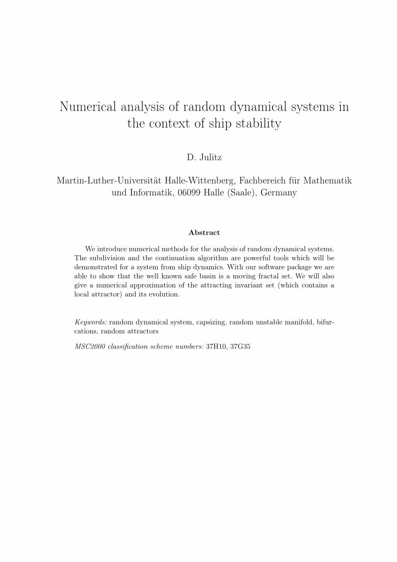
Figure 3.1: A single trajectory and an approximation of A(ω) of the Kramer-System.

The selection step has the task to decide which boxes of the actual family are already apart of the attractor. To make this decision we have to take the invariance property ofthe attractor into account. We take a box Bi of the actual family Bk after k subdivisionsteps and are searching their preimages φ−1(T, ω, Bi) for a suitable fixed timestep T

(this is to ensure a good convergence toward the random attractor and depends on thesystem) and a fixed ω. This means we are looking for the set of boxes

⋃

j∈J Bj where J

is the appropriate indexset, which will be at least mapped partly to our box Bi. If wefind at least one of these boxes in our actual cover, we can be sure that Bi is a part ofthe attractor. We have to do this for every box in the actual family Bk. Mathematicallyspeaking we can say we have to check for one box Bi

φ−1(T, ω, Bi) ∩ Bj = ∅

for all boxes Bj of the actual cover. If the intersection is empty then we know that Bi

is not a part of the attractor. In the other case it is. In general we are not able to mapcomplete boxes by the cocycle φ. To implement the algorithm we need a discretisationof boxes. A simple way to solve this problem is to choose a number of test points insideevery box.

The subdivision step and the selection step are coupled by two parts the initialisation

and the approximation part (see Figure 3.2). During the initialisation we perform n


108 D. Julitz

subdivision and selection steps. The result is a minimal number of valid boxes whichgives the actual cover of the attractor. In the second part we only perform selectionsteps to obtain a good approximation of the random attractor in the target fiber.

Figure 3.1 shows how powerful the subdivision algorithm works. In general a singletrajectory does not give a good understanding of the structure of a random attractorA(ω). Using the subdivision algorithm we get a clear picture of A(ω). We investigatedhere the Kramer-System with additive white noise. This system is given by the stochasticdifferential equation

x = x − δx − x3 + ε ξt ,

where ξt denotes a white noise process. Figure 3.1 is calculated for δ = 0.3 and ε = 0.5.

Ω

A(ω)

ApproximationInitialisation

Figure 3.2: The two parts of the algorithm.

The continuation algorithm

The continuation algorithm is able to approximate random unstable manifolds. It is verysimilar to the subdivision algorithm. Suppose our RDS is excited with multiplicativenoise and has an random unstable manifold with starting point in the origin.

Again we start with a box Q, which contains the random attractor with high probability.This algorithm is also separated into two parts. In the first part we divide the boxes upto a final level n. At this time all boxes are invalid. Then in the second part we activatethose boxes which cover the hyperbolic stationary random point. In the following weonly perform selection steps. All the boxes which covers the random unstable manifold


will be activated after some time. At the end the complete random unstable manifoldappears.

We illustrate the continuation algorithm by the well known deterministic Lorenz-Systemsee Figure 3.3. In this case the complete attractor appears after a while. This system isgiven by the differential equations

x = σ (y − x)

y = r x − x z − y

z = x y − b z.

Where σ = 10.0, b = 1.0 and r = 28.0. For these parameters the origin is an hyperbolicstationary point.


110 D. Julitz

Figure 3.3: Continuation of the hyperbolic origin of the Lorenz-System.


4 Results

We now want to apply the algorithms to a common system from ship dynamics to getsome insights about the structure of possible invariant object and bifurcation behaviour.Other numerical and analytical investigations of such systems are done for example in[2], [7], [9], [10], [14] and [15].

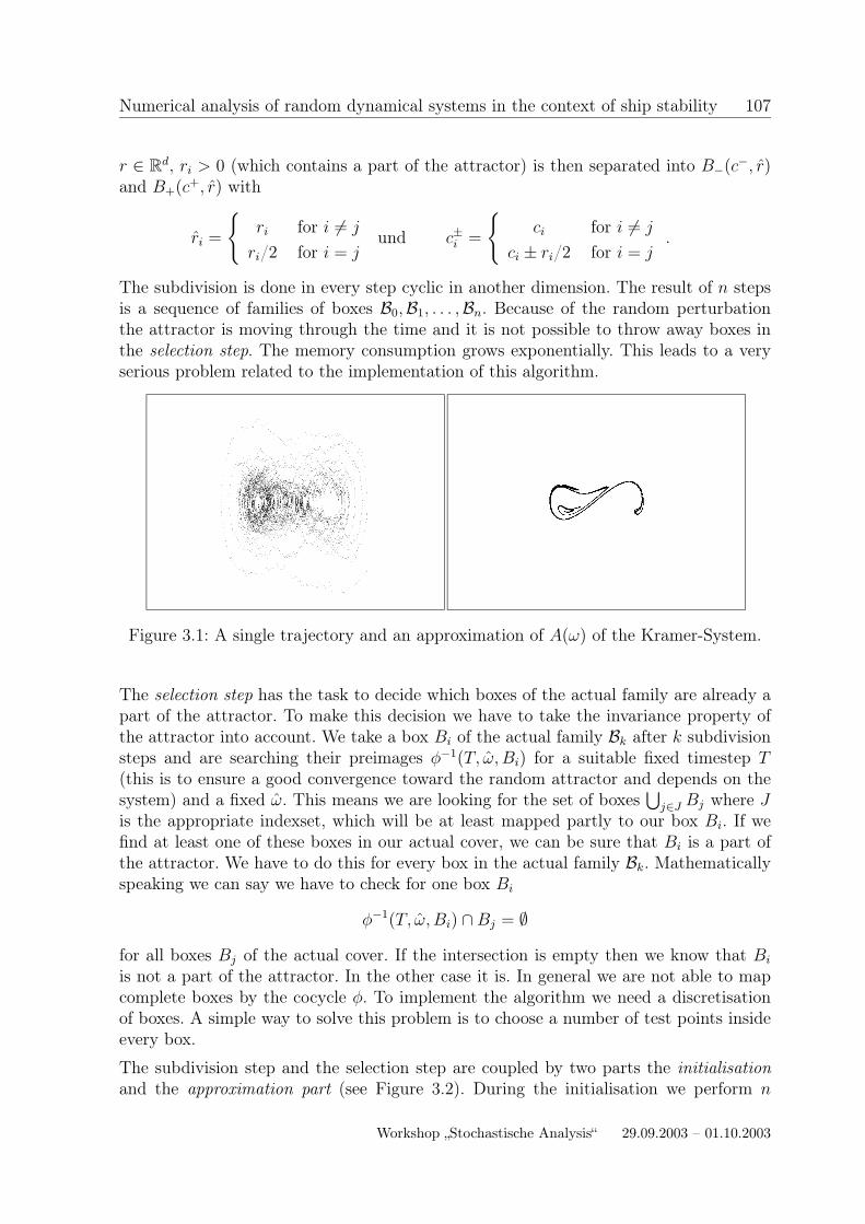
Figure 4.1: The attractor (left) and the safe basin (right) of the autonomous version ofsystem (4.1) with α = 0, β = 0.1 and Q = [−1.5, 1.5] × [−1.5, 1.5].

We will investigate the system given in [14]. This system describes the roll motion of aship and its capsizing. It is given by the periodic forced differential equation

x + βx + x(1 − x)(1 + αx) = F sin(0.85 t). (4.1)

Figure 4.2: Continuation of the stable manifold with origin in (1, 0) for the autonomousversion of system (4.1) with α = 0, β = 0.1 and Q = [−3, 3] × [−3, 3].

The capsizing is described here with the escape from a potential well [14]. This potentialwell depends on α. Common selections for α are 0, 1,−1, 1

2or −1

2. This system was


112 D. Julitz

investigated extensively for α = 0 and for α = −1. We will only consider the case α = 0here. Anyway there are no approximations of the attracting invariant set and its motionin time. In the papers we have seen, only the safe basin of attraction (erosion) wasexplored see [14] or [10]. This investigations was done only in one timefiber. The safe

basin corresponds to the set of initial conditions for which the corresponding trajectoriesremain near a local attractor. This means if we take the initial state for the ship fromthis set the ship will not capsize. When the periodic forcing is growing the safe basinbecomes a fractal structure (see Figure 4.4) and later it disappears completely. It is quitenatural that for large waves every ship will capsize.

Figure 4.3: Evolution of the attracting invariant set for the nonautonomous system (4.1)with α = 0, β = 0.1. In the first row we use F = 0.05 and in the second row F = 0.09with Q = [−1.5, 1.5] × [−1.5, 1.5] and 27 subdivisions.

Of course system (4.1) is a special RDS. It is possible to apply all the methods of Section 3to every type of nonautonomous dynamical system. The only thing to do is to implementthe type of perturbation with help of the MDS θ. Our software is able to generate anykind of perturbation. Hence we can analyse easily also periodic forced systems.

At first it seems to be a good idea to have a look at the autonomous version of system(4.1). In the autonomous case (F = 0) the attracting invariant set and the safe basinlook like in Figure 4.1. There exists a local attractor in the autonomous case. It is easy tosee that system (4.1) has two stationary points, the stable point (0, 0) and the hyperbolic


point (0, 1). The local attractor which attracts the safe basin consists of the stable point,the hyperbolic point and the manifold between them. The unstable unbounded manifoldwhich has its origin also in the hyperbolic point describes the capsizing of the ship (escapefrom the potential well). With continuation we can see that the stable manifold of thehyperbolic point is the boundary of the safe basin (see Figure 4.2).

Figure 4.4: Evolution of the safe basin for the nonautonomous system (4.1) with α = 0,β = 0.1. In the first row we used F = 0.05 and in the second row F = 0.09 withQ = [−1.5, 1.5] × [−1.5, 1.5] and 27 subdivisions.

For the evolution of the attracting invariant set in the nonautonomous case (F 6= 0) weobtain pictures similar to Figure 4.3. Here we used the perturbation ratios F = 0.05and F = 0.09. We can also get approximations of the safe basin if we calculate system(4.1) in negative time direction. The pictures of Figure 4.4 show typical evolutions ofthe safe basin for different F . In contrast to the deterministic case the local attractorand the safe basin seems to have a fractal structure for F large enough. It seems thesystem undergoes here a bifurcation with the wave height as bifurcation parameter. Theboundary of the safe basin for F = 0.09 is very complicated. The local attractor in theorigin for the unperturbed system (4.1) (F = 0) change to a more complicated randomattracting set (F = 0.05). The local random attractor seems to consist of more thanonly one stable random point near the origin. We obtain here a bifurcation scenario. Atthe end (F = 0.09) the safe basin becomes a fractal structure and the local attractor


114 D. Julitz

disappears. In this regime it makes no sense to speak about a safe basin anymore. Ingeneral the ship capsizes here.

We can also investigate a stochastic version of (4.1)

x + βx + x(1 − x)(1 + αx) = σ ξt (4.2)

with additive noise. Here ξt is a white noise process. Of course this is not a very realisticapproach for the problem of capsizing. White noise leads to the fact that the ship willcapsize with probability 1.

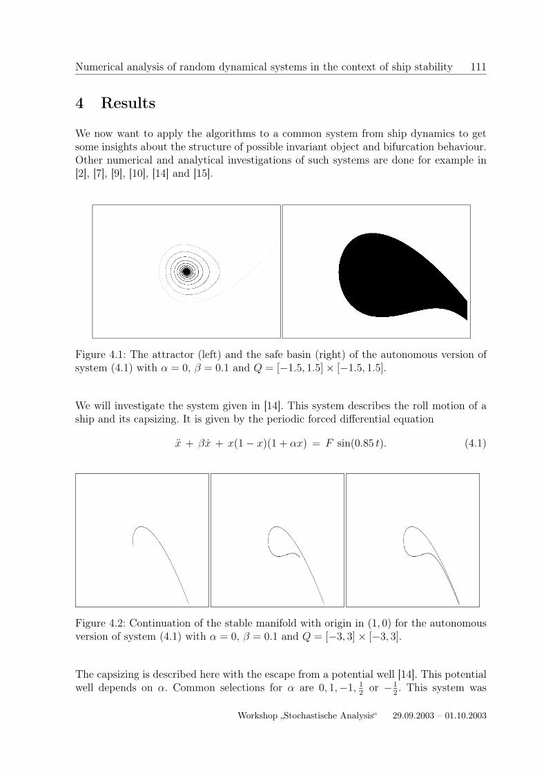
Figure 4.5: Evolution of the random attracting invariant set for the stochastic system(4.2) with α = 0, β = 0.1, σ = 0.1, Q = [−2, 2] × [−2, 2] and 27 subdivisions.

The results for the stochastic case are illustrated in Figure 4.5. We see again an evolutionof the random attracting invariant set which contains a local attractor. This randomattracting invariant set has also a fractal structure. But it seems that the local attractorconsist of only one random stable point. There is no bifurcation like in periodic case.

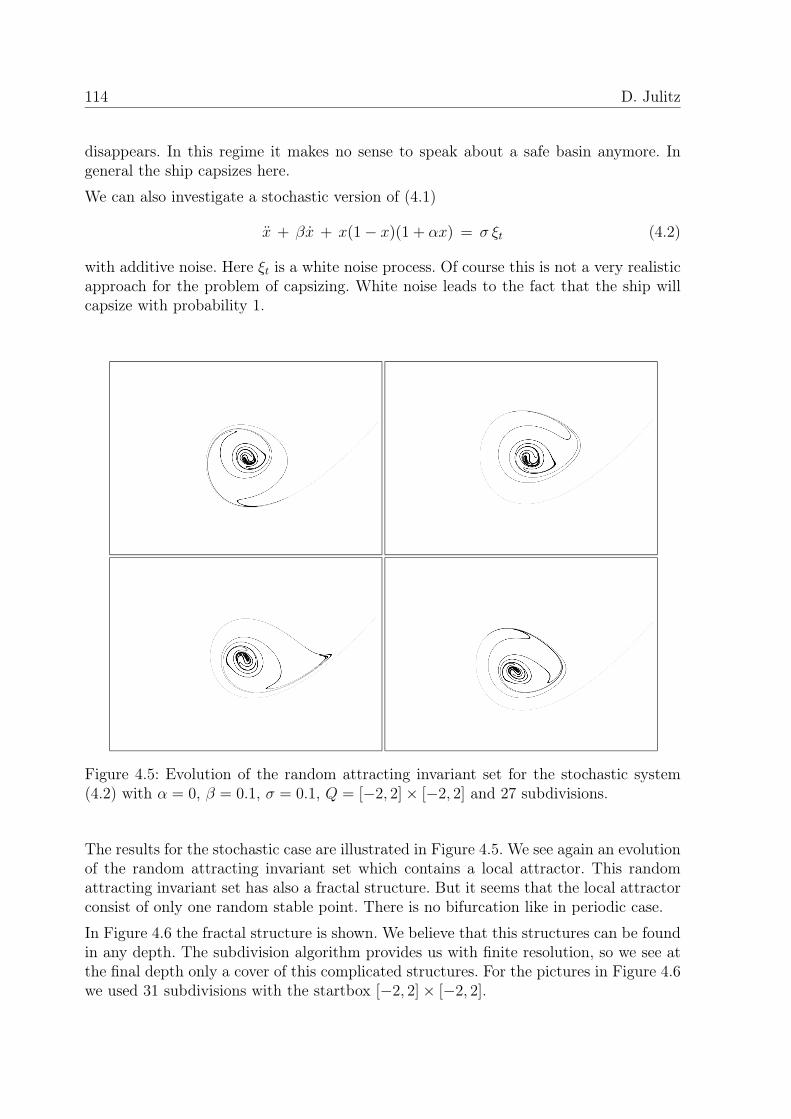
In Figure 4.6 the fractal structure is shown. We believe that this structures can be foundin any depth. The subdivision algorithm provides us with finite resolution, so we see atthe final depth only a cover of this complicated structures. For the pictures in Figure 4.6we used 31 subdivisions with the startbox [−2, 2] × [−2, 2].


Figure 4.6: Zoom into the random attracting set.


116 D. Julitz

5 Conclusion

The numerical methods we described in this article are useful tools for the numericalanalysis of nonautonomous systems. Applying these tools we can approximate invariantsets and investigate the evolution of these objects in time. We tried to apply our softwarepackage to a common model from ship dynamics. We are able to show effects like theerosion of the safe basin and the structure of the attracting invariant set for this systemwith a minimum of calculation. In general it takes only a few minutes to get pictureslike in Section 4 using a normal PC Pentium III class.

We intend to investigate more realistic models to get a better understanding of the globalbehaviour of real relevant models. In this context it is planned to analyse nonautonomousdynamical system which are generated by functional differential equations. Another pointis to use more realistic perturbations as sinuswaves or pure white noise.

References

[1] L. Arnold. Random Dynamical Systems. Springer Verlag, (1998).

[2] L. Arnold, I. Chueshov and G. Ochs. Stability and capsizing of ships in random sea.Institut für Dynamische Systeme, Universität Bremen (2003).

[3] M. Dellnitz and A. Hohmann. A subdivision algorithm for the computation of un-

stable manifolds and global attractors. Numerische Mathematik, 75:293-317, (1997).

[4] M. Dellnitz and A. Hohmann. The computation of unstable manifolds using sub-

division and continuation. Progress in Nonlinear Differential Equations and TheirApplications 19, Birkhäuser, pages 449-459, (1996).

[5] M. Dellnitz, G. Froyland, O. Junge. The Algorithms behind GAIO - Set Oriented

Numerical Methods for Dynamical Systems. Ergodic theory, analysis, and efficientsimulation of dynamical systems. Springer (2001).

[6] J. Duan and K. Lu and B. Schmalfuß. Invariant manifolds for stochastic partial

differential equations. Annals of Probability, Vol. 31, pages 2109-2135, (2003).

[7] H. Lin and C. S. Yim. Chaotic roll motion and capsize of ships under periodic

excitation with random noise. Ocean Engineering Program, Oregon State University,(1994).

[8] H. Keller and G. Ochs. Numerical approximation of random attractors. Institut fürDynamische Systeme, Universität Bremen, (1998).

[9] E. Kreuzer and M. Wendt. Ship capsizing analysis using advanced hydrodynamic

modelling. Phil. Tras. R. Soc. Lond. A, 358:1835-1851 (2000).


[10] Miguel A. F. Sanjuan. The effect of nonlinear damping on the universal escape

oscillator. Departamento de Ciencias Experimentales e Ingeniera, Universidad ReyJuan Carlos, Madrid, Spain, (1998).

[11] B. Schmalfuss. Backward cocycles and attractors of Stochastic Differential Equa-

tions. International Seminar on Applied Mathematics–Nonlinear Dynamics: Attrac-tor Approximation and Global Behaviour, pages 185-192, (1992).

[12] B. Schmalfuss. A random fixed point theorem and the random graph transformation.Journal of Mathematical Analysis and Applications, Vol. 225, Num. 1, pages 91-113,(1998).

[13] R. Temam. Infinite- Dimensional Dynamical Systems in Mechanics and Physics.Springer Verlag, (1997).

[14] M. Thompson. Designing against capsize in beam seas: recent advances and new

insights. American Society of Mechanical Engineers, 50:307-325, (1997).

[15] M. Wendt. Zur nichtlinearen Dynamik des Kenterns intakter Schiffe im Seegang.Fortschritt Berichte VDI, (2000).


numerical analysis of random dynamical systems in the ... · numerical analysis of random dynamical...

Documents