numerical analysis of tuned liquid dampers - kamalendu ghosh (09ce3112)

Numerical Analysis of Tuned Liquid Dampers

A thesis submitted to

Indian Institute of Technology, Kharagpur

In partial fulfillment for the award of the degree

of

Master of Technology in Civil Engineering

With specialization in

Structural Engineering

by

Kamalendu Ghosh (09CE3112)

Under the supervision of

Professor Arghya Deb

Department of Civil Engineering

Indian Institute of Technology Kharagpur

Kharagpur-721302, India

May 2014

i

DEPARTMENT OF CIVIL ENGINEERING

INDIAN INSTITUTE OF TECHNOLOGY

KHARAGPUR-721302

CETRIFICATE

This is to certify that the thesis entitled, “Numerical Analysis of Tuned Liquid Dampers” is a

bonafide record of authentic work carried out by Kamalendu Ghosh under my supervision and

guidance for the partial fulfillment of the requirement for the award of the degree of Master of

Technology in Structural engineering in the department of civil engineering at the Indian Institute of

Technology, Kharagpur.

The results embodied in this thesis have not been submitted to any other University or Institute for

the award of any degree or diploma.

Date: 02-05-2014

Place: Kharagpur

Dr. Arghya Deb

Associate Professor

Department of Civil Engineering

IIT Kharagpur

Kharagpur-721302

ii

Acknowledgement

With great pleasure and deep sense of gratitude, I express my indebtedness and profound gratitude

to Dr. Arghya Deb, Department of Civil Engineering, Indian Institute of Technology, Kharagpur

for his valuable guidance and constant encouragement at each and every step, from beginning of

this work. He exposed me to the research topic through proper counsel and rigorous discussions

and showed great interest in providing timely support and suitable suggestions.

I wish to convey my heartfelt thanks to all my friends for their encouragement and moral support

during the course of my project work.

Last but not the least I owe a great deal of indebtedness to my father who has been supporting me

throughout and is my greatest source of inspiration, strength and assurance.

iii

CONTENTS

1. INTRODUCTION ........................................................................................................... 1

1.1 PROBLEM DESCRIPTION ..................................................................................... 1

2. LITERATURE SURVEY ............................................................................................... 2

3. OBJECTIVES ................................................................................................................. 4

4. THEORETICAL BACKGROUNDS AND METHODOLOGY.................................... 5

4.1 Theoretical background............................................................................................. 5

4.2 Numerical study ......................................................................................................... 9

4.2.1 The Finite Element Model ................................................................................. 10

4.3 Hydraulic jump upon introduction of baffle .......................................................... 14

4.4 White noise ............................................................................................................... 14

5. VALIDATION ............................................................................................................... 15

5.1 Validation with displacement base excitation ......................................................... 15

5.2 Validation with rotational excitation ...................................................................... 15

6. RESULTS ...................................................................................................................... 17

6.1 Adoption of parameters to measure damping ........................................................ 18

6.2 Effect of mass of fluid in TLD on the damping parameters ................................... 19

6.3 Effect on damping due to introduction of baffle ..................................................... 22

6.3.1 Varying the location of the baffle with r=0.15m and A/L=0.01m .................... 23

6.3.2 Varying the amplitude of excitation with baffle location d=0 and r=0.15m .... 25

6.3.3 Varying the dimension of the baffle with location at d=0 and A/L=0.01 ......... 25

6.4 Effect on damping due to introduction of rectangular baffle................................. 27

6.5 FFT analysis on the response of the TLDs with baffles with white noise excitation

........................................................................................................................................ 30

6.5.1 Spectral width parameter ................................................................................. 31

6.6 Response to El-Centro and Koyna excitations ........................................................ 33

7. CONCLUSIONS ........................................................................................................... 35

8. REFERENCES .............................................................................................................. 36

iv

LIST OF TABLES

TABLE 1. PROPERTIES OF STRUCTURE ................................................................................... 12

TABLE 2. DIMENSIONS OF THE TANKS USED IN PRESENT STUDY .............................................. 17

TABLE 3. SPECTRAL WIDTH PARAMETERS FOR DIFFERENT TLD TYPES ................................... 32

TABLE 4. PERFORMANCE TO EL-CENTRO EXCITATION ........................................................... 34

TABLE 5. PERFORMANCE TO KOYNA EXCITATION ................................................................. 34

LIST OF FIGURES

FIGURE 1. SDOF STRUCTURE WITH TLD ATTACHED ON TOP ................................................... 5

FIGURE 2. SCHEMATIC SKETCH OF TLD MOTION ..................................................................... 7

FIGURE 3. THE MODIFIED TANK ............................................................................................ 13

FIGURE 4. THE STRUCTURE WITH TLD IN THE EULERIAN DOMAIN ......................................... 13

FIGURE 5. TIME HISTORY PLOT OF FREE SURFACE ELEVATION ON OUTER WALL OF A

RECTANGULAR TANK..................................................................................................... 15

FIGURE 6. TIME HISTORY OF FREE SURFACE ELEVATION ON THE RIGHT WALL OF THE TANK .... 16

FIGURE 7. EFFECT OF MASS A/L 0.01 .................................................................................... 20



FIGURE 10. TIME HISTORY OF DISPLACEMENT OF THE STRUCTURE WITH A CONCENTRATED LOAD

EQUAL TO THE WEIGHT OF THE TLD (M=0.1) AND THE STRUCTURE WITHOUT ANY LOAD. 22

FIGURE 11. TLD WITH SEMICIRCULAR BAFFLE ...................................................................... 23

FIGURE 12. EFFECT ON DAMPING PARAMETER D1 UPON INTRODUCTION OF BAFFLES ............... 24



FIGURE 15. EFFECT OF AMPLITUDE OF EXCITATION UPON DAMPING WITH BAFFLE................... 25

FIGURE 16. EFFECT ON DAMPING PARAMETER D1 UPON VARYING THE DIMENSION OF THE

BAFFLE ......................................................................................................................... 26


BAFFLE ......................................................................................................................... 26


BAFFLE ......................................................................................................................... 26

FIGURE 19. TLD WITH RECTANGULAR BAFFLE ...................................................................... 28

FIGURE 20. COMPARISON OF PERFORMANCE OF D1 BETWEEN RECTANGULAR BAFFLE AND

SEMICIRCULAR BAFFLE .................................................................................................. 28





FIGURE 23. APPLIED WHITE NOISE EXCITATION ..................................................................... 31

v

FIGURE 24. AUTOCORRELATION OF THE APPLIED WHITE NOISE SIGNAL .................................. 31

FIGURE 25. FFT ANALYSIS ................................................................................................... 32

vi

ABSTRACT

The next generation of tall structures are being designed to be lighter and more flexible, making

them susceptible to wind, ocean waves and earthquake type of excitations. One approach to

vibration control of such systems is through energy dissipation using a liquid sloshing damper.

Previous studies have shown that the TLD is most effective for a narrow band of frequency of

excitation. The purpose of this study is the numerical analysis of tuned liquid dampers with

the main objective of investigating the effect of mass of fluid on damping and devising methods

of increasing the effectiveness of Tuned Liquid Dampers over a wider range of excitation

frequencies.

In order to establish the effect of mass of fluid, numerical analysis was carried using the

ABAQUS finite element code using the coupled Eulerian-Lagrangian approach. Different

instances of the TLD was created each having different mass but tuned to the structural

frequency. Investigations were carried out by exciting the damped structure to different

excitations.

In order to increase the effectiveness of TLD over a broader spectrum of excitations baffles

were introduced into TLD. The structure with the modified TLD s were also excited to different

excitations. FFT analysis on the time history response of TLD with baffles to white noise

excitation was done to investigate the increase in effectiveness of TLD.

1

1. INTRODUCTION

The current trend of building structures of ever increasing height and the use of lightweight,

high strength material is often accompanied by increasing susceptibility to excitations such as

wind, ocean waves and earthquakes. To reduce the risk of structural failures, particularly during

a catastrophic event, it has become important to search for practical and effective devices for

suppression of these vibrations.

The devices used for suppressing the structural vibrations can be categorized according to their

energy consumption:

Passive Control

Active and Semi-active control

Hybrid system control system.

Passive control devices are systems that do not require external energy supply. Examples of

such systems include viscous dampers, tuned mass dampers, tuned liquid dampers, etc.

In TLDs the sloshing motion of the fluid that results from the vibration of the structure

dissipates a portion of the energy released by the dynamic loading and therefore increases the

equivalent damping of the structure. Tuned sloshing dampers can be classified into two

categories, shallow and deep water dampers based on the ratio of water depth to tank length in

the direction of motion. The TLD system relies on the sloshing wave developed at the free

surface of the liquid to dissipate a portion of the dynamic energy. The growing interest in TLDs

is due to their low capital and maintenance cost and their ease of installation in structures.

1.1 PROBLEM DESCRIPTION

TLDs are most effective only for a narrow frequency range of excitation. The damping due to

TLDs is highest when the excitation frequency is close to the tuned frequency. The main

purpose of this study is to devise methods to increase the effectiveness of TLD over a wider

band of frequencies of excitation. The effect of mass of damper on damping is also studied

here. It has also been attempted to devise parameters to quantify damping for any excitation.

2

2. LITERATURE SURVEY

Passive damping using TLDs is a challenging area of research and innovation and as such a

host of literature which covers this diverse area exists. Some references are summarized here

with a gist of their content.

Reed et al. (1998) concluded that the dissipation of vibration energy due to a TLD increases as

the excitation amplitude increases and the TLD behaves as hardening spring system. The

authors also said that to achieve a more robust system the design frequency for the damper, if

it is computed by the linearized wave theory, should be set at a value lower than that of the

structure response frequency, since this may result in the actual nonlinear frequency of the

damping matching the structural response. The authors also found that even if there damper

frequency is mistuned slightly, the TLD always performs well. They observed no adverse

effects due to slight mistuning.

Jin-Kyu et al. (1999) discusses the numerical modeling of a tuned liquid damper (TLD) as an

equivalent tuned mass damper with non-linear stiffness and damping. This non-linear stiffness

and damping (NSD) model captures the behavior of the TLD system adequately under a variety

of loading condition. In particular, NSD model incorporates the stiffness hardening property of

the TLD under a large amplitude excitation.

Yamamoto & Kawahar [16] considered a fluid model using Navier-Stokes equation in the form

of the arbitrary Lagrangian-Eulerian (ALE) Formulation. For the discretization of the

incompressible Navier-Stokes equation, they used the improved-balancing-tensor-diffusivity

method and the fractional-step method for computational stability.

Sun et al. (1992) proposed a nonlinear model for rectangular Tuned Liquid Damper. This model

utilizes the shallow water wave theory and is extended to account for the effect of breaking

waves by the introduction of two empirical coefficients determined experimentally.

Kareem et al. (2009) elaborated on the inherent non-linear behavior of the TLDs. The non-

linear behavior of the TLDs is characterized by an amplitude dependent frequency response

function, which translates into changes in frequency, as well as changes in the damping due to

sloshing, with amplitude. In this paper TLDs are modeled using a sloshing-slamming (S2)

analogy, which combines the dynamic effect of liquid sloshing and slamming/impact.

LITERATURE SURVEY

3

Banerji [3] conducted experimental and analytical analysis on a structure with TLD and

concluded that a 4% mass ratio and a 0.15 depth ratio enabled a TLD to be most effective for

broad-banded ground motion. This optimal TLD can reduce the response of a SDOF structure

typically by about 30%, which is sufficient from a design point of view.

Modi et al. [11] investigated on enhancing the energy dissipation efficiency of a rectangular

liquid damper through introduction of two dimensional wedge shaped obstacles. From the

experiment he concluded that wedging increases damping factor and damping factor further

increases for a roughened wedge.

Modi and Munshi [12] conducted parametric study with rectangular sloshing dampers in the

presence of semi-circular obstacles and wind tunnel tests and observed higher damping over

an extended range of frequencies.

4

3. OBJECTIVES

This project is confined to the investigations on a shallow water TLD.

The objectives of this project are:

i. Investigation into the effect of mass ratio on damping of a shallow TLD.

ii. Investigate into the performance of a shallow TLD with varying the non-dimensional 𝐴

𝐿

1 ratio and frequency of excitation.

iii. Devise parameters to quantitatively measure the effectiveness of TLDs.

iv. Enhance the performance of TLD over a wider spectrum of frequency of excitation with

the use of baffles.

1 A= amplitude of excitation, L=length of the tank in the direction of liquid sloshing

5

4. THEORETICAL BACKGROUNDS AND METHODOLOGY

4.1 Theoretical background

Figure 1. SDOF structure with TLD attached on top

The structure and the TLD can be modelled as a classical single degree of freedom system as

shown in Fig. 1. This system when subjected to a ground motion characterized by ground

acceleration ag, the equation of motion of the structure is written as:

( )s wm m sx

+ sc sx

+ ( )s s s w gk x m m a F

(1)

where sm , wm , sk , sx and sc represent mass of the structure, mass of water, stiffness, relative

displacement of the lumped mass with respect to the ground and damping coefficient of the

structure respectively. Eq. (1) can also be written as:

sx

+ 2 s s sx

+ 2

s sx g

s w

Fa

m m

(2)

6

where s and s are the structural damping and circular frequency respectively. The TLD base

shear force F is the hydrodynamic force induced by liquid sloshing which is calculated from

the shallow-water wave theory.

THEORETICAL BACKGROUNDS AND METHODOLOGY

7

2 21[ ]

2r lF gb h h (3)

where =density of liquid, b = breadth of tank, rh and rh are as shown in Fig. 2.

Figure 2. Schematic sketch of TLD motion

Shallow-water wave theory

The shallow-water wave theory is based on the depth-averaged equations of mass (equation of

continuity) and momentum conservation. This formulation assumes that the liquid is

incompressible and inviscid, and that the water depth is very small in comparison to the

characteristic length scale of motion. The equations of mass and momentum conservation are

0h u

t x

(4)

0

u uu g

t x x

(5)

where u =horizontal velocity, g =acceleration due to gravity, and h are as shown in Fig. 2.

The shallow-water wave propagates with a speed independent of its wavelength (non-

dispersive) but is dependent on its amplitude. The models which are based on non-dispersive

non-linear shallow-water wave equations can quite aptly model the wave breaking and energy

dissipation (Lamb 1932). This is the reason why shallow-water wave theory was selected to

model sloshing in a TLD.


8

Basic TLD equations

The rigid TLD tank (Fig. 2) when subjected to horizontal base motion sx the equations of

sloshing are given by the continuity equation

0

u w

x z

(6)

and the two dimensional Navier Stokes equations:

2 2

2 2

1s

u u u p u uu w x

t x z x x z

(7)

2 2

2 2

1w w w p w wu w g

t x z z x z

(8)

( , , )u u x z t , ( , , )w w x z t are the velocities of liquid particles relative to tank in x and z

directions respectively and is the kinematic viscosity of the liquid. Based on shallow water

wave theory the velocity potential, is assumed to be

( , , ) ( , ) cosh( ( ))x z t F x t k h z (9)

where k is the wave number. The boundary conditions are

0u on the end walls ( )x a (10)

0w on the bottom ( z h ) (11)

w u

t x

on the free surface ( 0z ) (12)

op p on the free surface ( 0z ) (13)

When the governing differential equations are integrated with respect to z from tank bottom to

the free-surface, the following equations are obtained:

( )0

uh

t x

(14)

22

2(1 )H s

u uT u g gh u x

t x x x x

(15)

where tanh( ) / ( )kh kh , tanh( ( )) / tanh( )k h kh and tanh( ( ))HT k h . It should be

noted that in arriving these equations the viscosity term in the governing equations are dropped.


9

The fundamental natural frequency of water sloshing predicted by linear water theory (Lamb

1932) is given by

1tanh

2w

g hf

L L

(16)

where L= length of tank in the direction of liquid sloshing, h

L= depth ratio

Shallow water and deep water TLD

In case of shallow water dampers h

L ratio is limited to 0.15, thus water depths required for

short period structures from the above equation are too small for practical application. The

frequency of sloshing is given by Eq. (16).

Fundamental frequency of deep water dampers (with h

L >1) is given by:

1

2w

gf

L

(17)

Thus the fundamental frequency of sloshing for deep water TLD is independent of the depth

ratio.

4.2 Numerical study

To study the objectives of the current study a numerical model of the set up was created using

the commercially available finite element code ABAQUS and several numerical simulations

were performed.

In TLDs, the motion of the liquid, especially at the free surface, can result in extreme

deformations. This will result in severe mesh deformation as well. This will cause the Jacobian

to become very small or even negative. A negative determinant of the Jacobian matrix would

cause the analysis to terminate. In order to prevent this, and to permit simulation of large

amplitude sloshing motions, a coupled Lagrangian-Eulerian approach was adopted.


10

In contrast to a Lagrangian analysis, where the Lagrangian elements comprise a single material

only, in an Eulerian analysis the Eulerian elements may not always comprise of a single

material: many may be partially or filled with air i.e. void. The Eulerian material boundary

must, therefore, be computed during each time increment and generally does not correspond to

an element boundary. The recomputed material boundaries must ensure conservation of mass,

momentum and energy.

In addition, the nodes in an Eulerian finite element mesh are fixed in space, unlike in the

Lagrangian case where the nodes move with the material. The Eulerian mesh is typically a

simple rectangular grid of elements constructed to extend well beyond the Eulerian material

boundaries, giving the material space in which to move and deform. If any Eulerian material

moves outside the Eulerian mesh, it results in loss of mass from the simulation, and in the

present application at least, in accurate results.

Unlike the liquid in the tank, the tank and its walls undergo limited motions. A Lagrangian

finite element analysis is therefore adopted for these parts. But at the liquid structure interface,

it is necessary to reconcile the two different formulations through Eulerian-Lagrangian

Contact. In this approach, at the interface the liquid motion results in traction forces at the

boundary of the solid, while the displacements of the solid result in displacement or velocity

boundary conditions for the liquid.

The TLD was therefore modeled using the coupled Eulerian-Lagrangian capability in

ABAQUS/Explicit.

4.2.1 The Finite Element Model

4.2.2.1 The Liquid

The water was modelled using EC3D8R Eulerian elements and a linear Us-Up equation of state

(EOS) material. In a linear Us-Up material the bulk modulus K is calculated as

2

0K c (18)

where is the density of water and 0c is the speed of sound in liquid. Since water is

incompressible, its bulk modulus is calculated using Eq. (18) is very high. This is a problem,


11

since in an explicit time integration algorithm the stable time increment is inversely

proportional to material bulk moduli. As a consequence, the stable time increment for the

analysis becomes excessively small resulting in unrealistically high solution times, given the

computational resources available. To ensure practical turnaround times for the analysis, 0c

was not taken as its actual value of 1460 ms-1. Instead, a reduced value of two orders of

magnitude smaller was used for simulations. This reduced the bulk modulus of the liquid,

thereby increasing the stable time increment and allowing the simulations to be completed in a

realistic time frame. Similar strategies adopted by other authors for coupled Eulerian-

Lagrangian analysis have substantiated little significant difference in the results. Though the

analytical formulations of linear sloshing theory described in Section 4.1 assumes the liquid to

be incompressible, the reduction in bulk density results in the introduction of slight

compressibility to the fluid. But as the comparison with the benchmark solutions described in

Chapter 5 indicate, this does not appear to be making any significant difference to the results.

A small viscosity of magnitude of 1.E-5 2N sm was also added in order to damp out high

frequency noise in the numerical solution, despite the assumption that the water is inviscid.

Again, the comparisons with the benchmark solutions indicate no significant difference in

result.

4.2.2.2 The Tank

The tank was modelled using C3D8R solid elements and were converted to rigid bodies to save

computational time, since deformation of the tank and its walls do not significantly affect the

sloshing motion.

4.2.2.3 Interactions

The penalty method is used to enforce contact between the Lagrangian solids and the Eulerian

liquid. In the penalty method, interpenetrations between two contacting surfaces are prevented

by penalty forces. The magnitude of penalty forces depend on the magnitude of penetration.

The penalty stiffness, if adequately chosen, prevents interpenetration between the contacting

parts.

The sloshing motion of the liquid will result in impact between the liquid and the tank walls.

Hence, contact between the Eulerian liquid material and the solid parts were enforced using the

penalty contact based General Contact capability in ABAQUS/Explicit. The contact penalties


12

were the default penalties calculated by ABAQUS, which are the maximum possible penalty

stiffness values that can be used without further reducing the stable time increment.

4.2.2.4 Modifications

Leakage of the liquid from the tank was witnessed during initial simulations of the TLD under

gravity load. Several modifications were incorporated to minimize such undesirable leakages.

Fillets were added to the sharp corners of the tank walls and additional layers of tank walls

were introduced. Fillets helped remove the singularity in the surface normal at sharp corners in

the tank walls, while additional layers of tank walls provided the extra contacting surfaces that

trapped any leaked material, thereby “blocking” the leaks and limiting escape of any further

material from the tank.

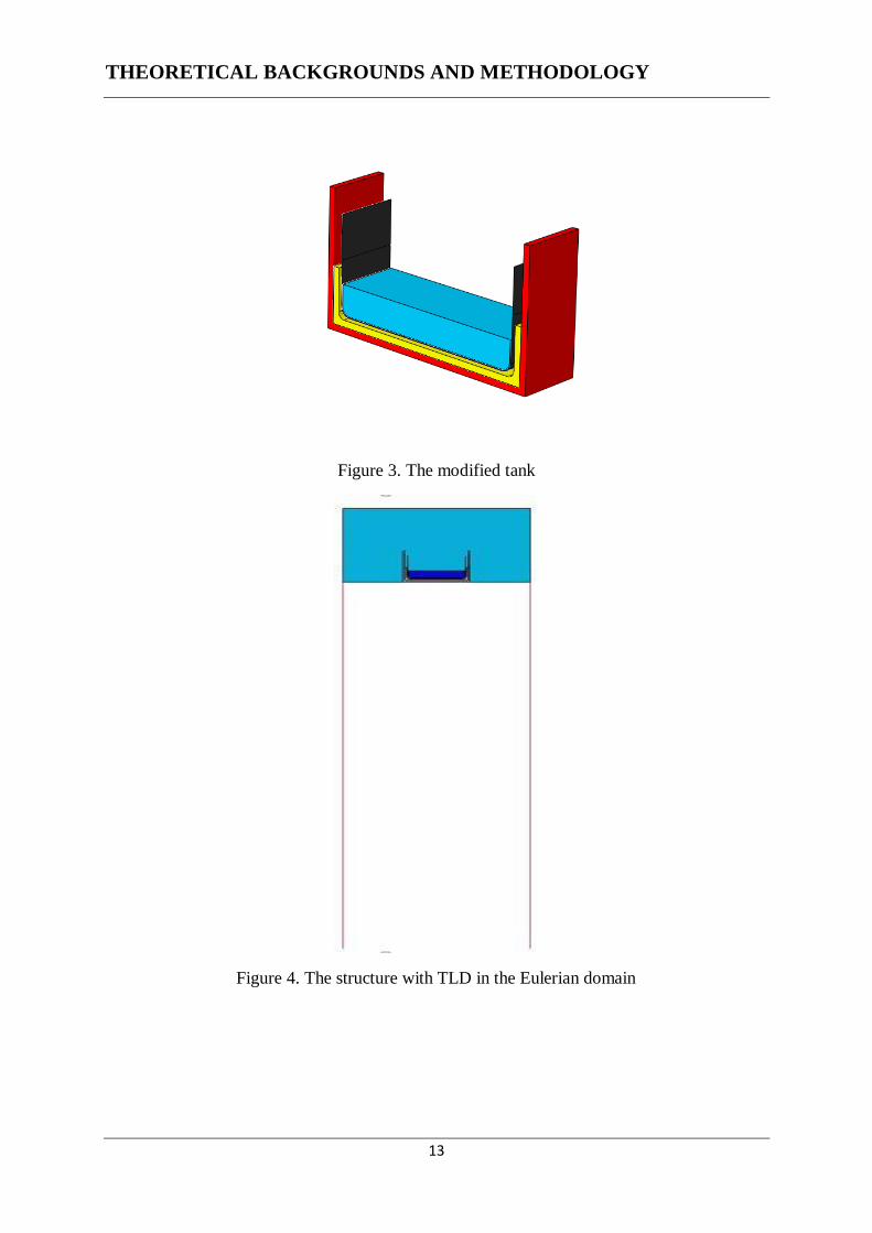
4.2.2.5 The Structure

A single bay portal frame chosen as the structure for all the analysis with TLD was modeled

using 2-D beam elements. The dimensions and other data of the structure are shown in Table

1.

Table 1. Properties of structure

Length of beam 10 m

Length of columns 25m

Cross-sectional area

Beam 0.3m x 0.3m

Column 0.8m x 0.8m

Density 2400kg m-3

Weight of the structure 78.96 ton


13

Figure 3. The modified tank

Figure 4. The structure with TLD in the Eulerian domain


14

4.3 Hydraulic jump upon introduction of baffle

A baffle at the bottom of the tank may contribute to additional energy dissipation by inducing

a hydraulic jump at the location of the baffle. Modi and Munshi [12] tested this idea with a

baffle of semi-circular cross section.

4.4 White noise

Excitation of a structure using white noise for system identification is widely quoted in

literature. Kondo and Hamatoto [10] illustrates a similar use.

White noise is a random signal with constant power spectral density. It also refers to a discrete

signal whose samples are regarded as a sequence of uncorrelated random variables with zero

mean and finite variance. The samples are independent and have the same probability

distribution. If each sample has a normal distribution with zero mean, the signal is said to be

Gaussian white noise.

15

5. VALIDATION

The numerical model was validated by solving two well-known benchmark problems. The

results obtained were compared with those obtained by Nakayama [13] and Biswal [4]. The

ABAQUS manual contains a solution for the problem solved by Nakayama, but it uses the ALE

(Arbitrary Lagrangian Eulerian) procedure for the solution. The solution obtained using the

current Coupled Eulerian Lagrangian procedure compared well with the ALE results as well.

5.1 Validation with displacement base excitation

To validate the numerical model, sloshing behavior of liquid in a partially filled rectangular

tank was investigated under sinusoidal base excitation. The same problem was investigated by

Nakayama et al. (1981) [13] using boundary element method and by Biswal et al. (2003) [4]

by finite element method. For the benchmark study, a rectangular tank with 0.9m base width

and filled with liquid up to 0.6m was considered under sinusoidal horizontal base acceleration

of 2

0 sin( )x x t in the X direction. The values of ox and were taken as 0.002m and

5.5 rad/sec respectively, as considered by the studies of Nakayama et al. and Biswal et al.

Figure 5. Time history plot of free surface elevation on outer wall of a rectangular tank

5.2 Validation with rotational excitation

ABAQUS Benchmark Problem

-80

-60

-40

-20

0

20

40

60

0 2 4 6 8 10

He

igh

t o

f w

ave

( m

m)

Time (s)

Present Nakayama Biswal

VALIDATION

16

A rigid tank measuring 90 x 80 x 60 cm initially inclined 0.8 degrees with respect to the y-axis

and filled with water up to a height of 60 cm, was rotated abut a point midway at water surface

between the two tank walls. The applied rotation was:

0.01396cos(5.5 )t (19)

The slosh height on the right wall of the tank was compared to numerically obtained reference

solution given by Nakayama and Washizu (1980).

Figure 6. Time history of free surface elevation on the right wall of the tank

-6.00E-02

-4.00E-02

-2.00E-02

0.00E+00

2.00E-02

4.00E-02

6.00E-02

8.00E-02

0 2 4 6 8 10 12 14

Hei

ght

of

wav

e (m

m)

Time (s)

Nakayama and Washizu Current Study

17

6. RESULTS

The first eigen frequency of the structure was computed. With the objective of studying the

effect of mass of the fluid in the TLD four different tanks with different masses tuned to the

structural frequency were designed by varying the depth ratio (Eq. (16)).

Table 2. Dimensions of the tanks used in present study

Mass ratio Length of the tank (L) Height of water (h) ℎ

𝐿

0.0122 1.5 m 0.110m 0.073

0.02931 2.0 m 0.192m 0.096

0.05829 2.5 m 0.305m 0.122

0.10000 3.0 m 0.450m 0.150

TLD s with different masses tuned to the same structural frequency could also have been set

up by changing the density of fluid in the tank. However changing the density of the fluid

would require using a fluid other than water in the tank. Hence this is not desirable.

Dynamical systems subjected to sinusoidal excitations shows sinusoidally varying steady state

response. In the presence of damping, the amplitude of the response is considerably smaller

than the response of the undamped system. The damped response for such excitations can be

easily computed using parameters such as the deformation response factor Rd, the velocity

response factor Rv, and the acceleration response factor Ra where Rd is the dynamic

magnification factor ratio and Rv and Ra are defined in terms of Rd and the constant β as

follows:

Rv= βRd

Ra= β2Rd

However if the TLD is subjected to random excitation, the response is a combination of many

different frequencies. Hence the damping parameters defined above are not directly applicable.

Hence to quantify damping performance of TLDs, it becomes imperative to device alternative

parameters to measure the reduction in the response of damped system.

The advantage in a numerical simulation is that these parameters can be derived quantities –

RESULTS

18

they need not only be primary variables like displacement, velocity or acceleration which are

experimentally measurable and are therefore preferred in most experimental studies. One

derived quantity which is easily available as an output quantity in a numerical solution is the

energy of the system. If one can get some idea of the distribution of the total energy of the

system among its several components, and the manner in which this distribution evolves with

time, it may be possible to use these energy quantities as a measure of the extent of damping.

For example if one finds that the kinetic energy and internal energy of a component of a damped

system are substantially reduced from their benchmark value, one can reliably conclude that

the damping mechanism (e.g. a TLD) has been more effective in this case than in the

benchmark.

6.1 Adoption of parameters to measure damping

With the above objective in view, in the present work, three parameters are proposed to

measure the influence of damping. The first parameter is based on a primary variable, the

displacement of a point on the structure, while the other two are derived quantities and are

based on the energy of the system. The parameters are:

i. Percentage reduction in maximum absolute displacement (d1)

ii. Percentage reduction in total internal energy (d2)

iii. Percentage reduction in total kinetic energy (d3)

The parameters are defined by Eq. (20), Eq. (21) and Eq. (22) respectively.

The parameter d1 is a measure of the maximum deformation that the structure undergoes till

the termination of the excitation. Total internal energy is the total strain energy of the structure

during the excitation period. Total KE is the measure of the energy associated with velocity of

sway and can be a measure of the degree of discomfort experienced by the residents of the

structure.

The studies on the response of the structure with and without TLDs will be a test of the

effectiveness of these parameters in quantifying damping as well.

RESULTS

19

maxmax

1

max

100d d

dd

(20)

2 100

tottot

tot

IE IEd

IE

(21)

3 100

tottot

tot

KE KEd

KE

(22)

where, maxd = maximum absolute displacement of the undamped structure

maxd = maximum absolute displacement of the damped structure

totIE = time integral of internal energy into the undamped structure at the end of

excitation

tot

IE = time integral of internal energy into the damped structure at the end of

excitation

totKE = time integral of kinetic energy into the undamped structure at the end of

excitation

tot

KE = time integral of kinetic energy into the damped structure at the end of

excitation

6.2 Effect of mass of fluid in TLD on the damping parameters

Each TLD whose performance characteristics were to be measured were attached to the top of

the structure and subjected to sinusoidal excitations with varying frequency ratios (β) and non-

dimensional amplitudes of excitations ( ).

The value of λ was kept less than equal to 0.03 in order to confine sloshing within the zone of

“weak breaking”.[6]

RESULTS

20

𝜆 =

𝐴𝑚𝑝𝑙𝑖𝑡𝑢𝑑𝑒 𝑜𝑓 𝑒𝑥𝑐𝑖𝑡𝑎𝑡𝑖𝑜𝑛

𝐿𝑒𝑛𝑔𝑡ℎ 𝑜𝑓 𝑡ℎ𝑒 𝑡𝑎𝑛𝑘 𝑖𝑛 𝑡ℎ𝑒 𝑑𝑖𝑟𝑒𝑐𝑡𝑖𝑜𝑛 𝑜𝑓 𝑙𝑖𝑞𝑢𝑖𝑑 𝑠𝑙𝑜𝑠ℎ𝑖𝑛𝑔 (23)

𝛽 =

𝐸𝑥𝑐𝑖𝑡𝑎𝑡𝑖𝑜𝑛 𝑓𝑟𝑒𝑞𝑢𝑒𝑛𝑐𝑦

𝑇𝑢𝑛𝑒𝑑 𝑓𝑟𝑒𝑞𝑢𝑒𝑛𝑐𝑦 (24)

The value of λ was of the parameters defined in the previous section.

Figure 7. Effect of mass A/L 0.01


-50

0

50

100

0.6 0.8 1 1.2 1.4

d1

frequency ratio-100

-50

0

50

100

0.6 0.8 1 1.2 1.4

d2

frquency ratio

-50

0

50

100

150

0.6 0.8 1 1.2 1.4

d3

frequency ratio

-20

0

20

40

60

80

100

0.6 0.8 1 1.2 1.4

d1

frequency ratio

-50

0

50

100

150

0.6 0.8 1 1.2 1.4

d3

frequency ratio

-100

-50

0

50

100

150

0.6 0.8 1 1.2 1.4

d2

frequency ratio

RESULTS

21

From the results in Fig. 7, Fig. 8 and Fig. 9, it can be concluded that the performance of the

damping parameters are consistent with each other for all excitation scenarios: an increase in

the maximum absolute displacement is accompanied by an increase in the kinetic energy as

well as in the internal energy. Thus the damping parameters defined above can be used as a

measure of damping.

The results also show that for all cases the TLDs are most effective at excitation frequencies

that are close to the natural frequency of the structure. However, the performance drops as the

value of β shifts from 1.0.

The effect of the mass of damper is also evident from the figures. Higher mass ensured

enhanced damping at β close to 1. But is the increase in the value of the damping parameters

with increased mass of damper truly due to increase in sloshing? In order to verify this, a

simulation where a gravity load equal in magnitude to the gravity load due to the additional

mass of the damper was applied to the top of the structure. The response of the structure with

the concentrated load, and that of the structure without concentrated load, showed no

difference. This clearly indicated that the increase in damping experienced by the structure with

increased fluid mass was due to fluid sloshing. (Fig. 10)


-50

0

50

100

150

0.6 0.8 1 1.2 1.4

d1

frequency ratio-100

-50

0

50

100

150

0.6 0.8 1 1.2 1.4

d2

frequency ratio

-50

0

50

100

150

0.6 0.8 1 1.2 1.4

d3

frequency ratio

RESULTS

22

It is however also clear from Fig. 7–9 that the effectiveness of TLDs with higher water mass

decrease as the excitation frequency shifts from the tuned frequency. Thus increase in fluid

mass results in an increase in the effectiveness of the TLD over a narrower range of excitation

frequencies.

Figure 10. Time history of displacement of the structure with a concentrated load equal to the

weight of the TLD (m=0.1) and the structure without any load.

6.3 Effect on damping due to introduction of baffle

As seen in Section 6.2 the tank with the highest mass ratio showed the best damping

characteristics at frequencies close to the natural frequency of the structure. However at

frequencies away from the natural frequency, there was significantly less damping. In an

attempt to improve the damping performance of this tank, two semicircular baffles of radii

0.15m and 0.2 m were introduced at the bottom of the tank. As mentioned in Section 4.3

previous research [12] indicates that a baffle at the bottom of the tank may contribute to

additional energy dissipation. The purpose of the simulations was to explore whether the

additional energy dissipation due to the baffle succeeds in extending the damping performance

of the TLD with the highest mass ratio over a wider frequency range.

Analysis were performed for three different baffle locations:

i. d = 0 ii. d = 0.25l iii. d = 0.50l,

where d = distance of the center of the baffle from the center of the tank and, l = 𝐿

2, L= 3m.

RESULTS

23

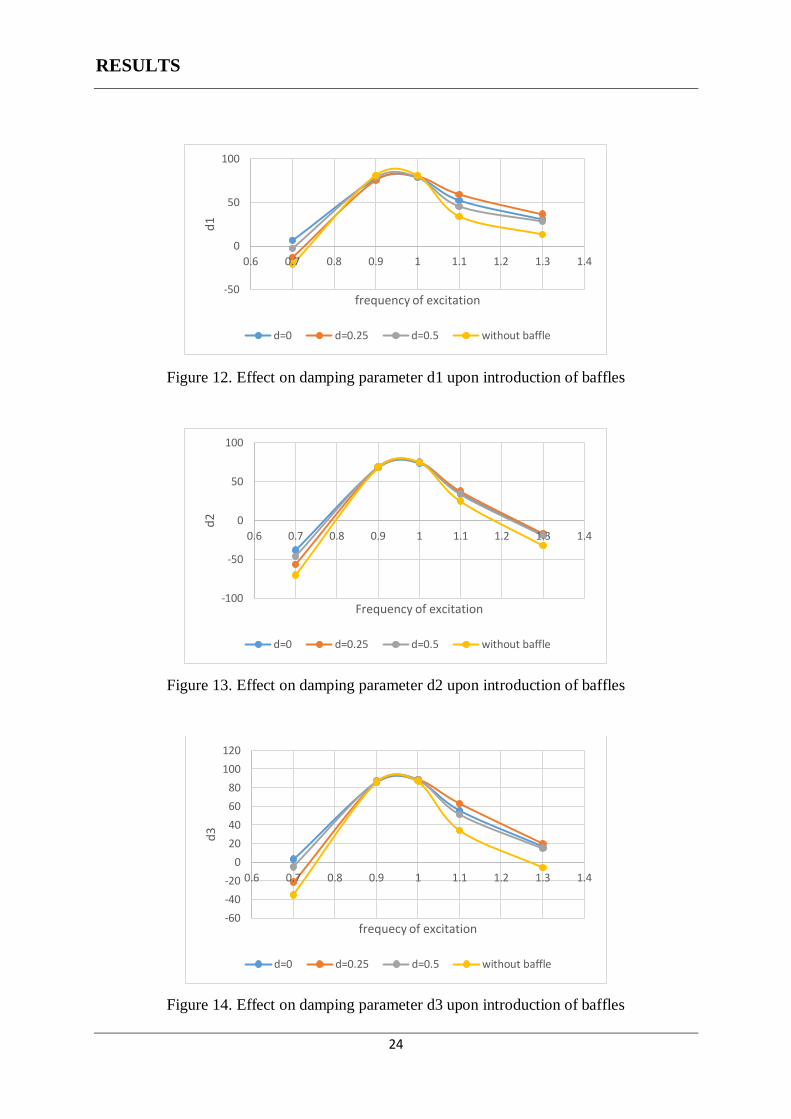
Fig. 11. shows the TLD with a semicircular baffle. Fig. 12-18 shows the performance of the

three damping parameters for this baffle for sinusoidal excitations as in the previous section.

Figure 11. TLD with semicircular baffle

The results are shown in the following sections.

6.3.1 Varying the location of the baffle with r=0.15m and A/L=0.01m

Fig. 12-14 illustrate the effect of varying the location of the baffle keeping the dimension and

the amplitude of excitation constant. . It was observed that while the performance for all the

three locations were nearly the same for frequency close to the tuned frequency, the TLD with

baffle at the center of the tank gave better results for other values of frequency ratio.

As Section 6.2, the performance of the damping parameters are again consistent with each other

for all excitation scenarios- an increase in the maximum absolute displacement is accompanied

by an increase in the kinetic energy as well as in the internal energy.

RESULTS

24

Figure 12. Effect on damping parameter d1 upon introduction of baffles



-50

0

50

100

0.6 0.7 0.8 0.9 1 1.1 1.2 1.3 1.4

d1

frequency of excitation

d=0 d=0.25 d=0.5 without baffle

-100

-50

0

50

100

0.6 0.7 0.8 0.9 1 1.1 1.2 1.3 1.4

d2

Frequency of excitation


-60

-40

-20

0

20

40

60

80

100

120

0.6 0.7 0.8 0.9 1 1.1 1.2 1.3 1.4

d3

frequecy of excitation


RESULTS

25

6.3.2 Varying the amplitude of excitation with baffle location d=0 and r=0.15m

Increasing the amplitude of excitation increases the velocity of waves and hence increases

energy dissipation due to enhanced hydraulic jump.

∆d= 𝐷𝑎𝑚𝑝𝑖𝑛𝑔 𝑐𝑎𝑢𝑠𝑒𝑑 𝑏𝑦 𝑡ℎ𝑒 𝑇𝐿𝐷 𝑤𝑖𝑡ℎ 𝑏𝑎𝑓𝑓𝑙𝑒−𝐷𝑎𝑚𝑝𝑖𝑛𝑔 𝑐𝑎𝑢𝑠𝑒𝑑 𝑏𝑦 𝑡ℎ𝑒 𝑇𝐿𝐷 𝑤𝑖𝑡ℎ𝑜𝑢𝑡 𝑏𝑎𝑓𝑓𝑙𝑒

𝐷𝑎𝑚𝑝𝑖𝑛𝑔 𝑐𝑎𝑢𝑠𝑒𝑑 𝑏𝑦 𝑡ℎ𝑒 𝑇𝐿𝐷 𝑤𝑖𝑡ℎ𝑜𝑢𝑡 𝑏𝑎𝑓𝑓𝑙𝑒x100

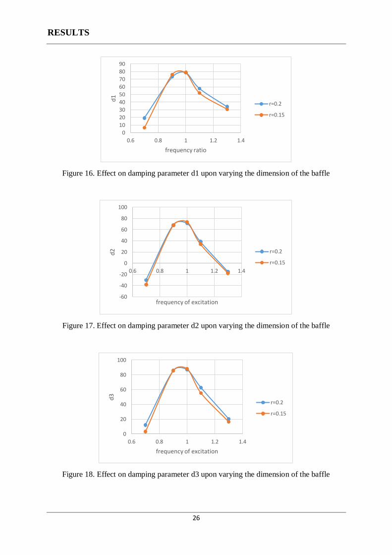
6.3.3 Varying the dimension of the baffle with location at d=0 and A/L=0.01

It can be concluded from the results shown in Fig. 16, 17 and 18, that to increase the

effectiveness of a TLD over a wider range of excitation frequencies, a semicircular baffle with

larger radius is preferable. Since, the damping parameters at frequency ratios close to 1 for both

the TLD s are almost the same, larger baffles are even the more favorable, since it does not

compromise with the performance for excitations tuned to the natural frequency while being

more effective over a wider range of excitation frequencies.

Figure 15. Effect of amplitude of excitation upon damping with baffle

-50

0

50

100

150

200

250

0.6 0.8 1 1.2 1.4

∆d

1

frequency ratio-50

0

50

100

150

200

250

0.6 0.8 1 1.2 1.4

∆d

2frequency ratio

-200

0

200

400

600

800

1000

0.6 0.8 1 1.2 1.4

∆d

3

frequency ratio

RESULTS

26

Figure 16. Effect on damping parameter d1 upon varying the dimension of the baffle



0

10

20

30

40

50

60

70

80

90

0.6 0.8 1 1.2 1.4

d1

frequency ratio

r=0.2

r=0.15

-60

-40

-20

0

20

40

60

80

100

0.6 0.8 1 1.2 1.4

d2


r=0.2

r=0.15

0

20

40

60

80

100

0.6 0.8 1 1.2 1.4

d3


r=0.2

r=0.15

RESULTS

27

6.4 Effect on damping due to introduction of rectangular baffle

Presence of semicircular baffle thus increased the effectiveness over a larger frequency range.

It was argued that rectangular baffles would further enhance the effectiveness of TLD, as the

tank would behave as a Multiple Tuned Liquid Damper (MTLD) till the water depth equal to

the height of the baffle.

The frequency of sloshing in shallow water TLD is very sensitive to the depth ratio. A

rectangular baffle divides the entire length of the tank in two parts. Hence it was reasoned that

till a water height equal to the height of the baffle the TLD would have a frequency of sloshing

obtained using the divided lengths of the tanks, while most of the water in the tank would slosh

with a frequency obtained using the entire length of the tank. Thus it was hoped that

introduction of rectangular baffle would have multiple dominant frequencies of sloshing.

Three rectangular baffles were created with constant breadth while varying the height. The

performance of the TLD with these rectangular baffles were compared with the TLD with a

semicircular baffle of radius, r=0.2m. The dimensions of the rectangular baffles considered

were:

i. Breadth (b) =0.4m, height (h0=0.1 m).

ii. Breadth (b) =0.4m, height (h0=0.2 m).

iii. Breadth (b) =0.4m, height (h0=0.3 m).

Fig. 20-22 compares the performance of the rectangular baffle with the performance of the

baffle of radius 0.2m which performed better than the semicircular baffle of radius 0.15m in

the previous analysis. The dimensions of the baffle were chosen such that the breadth of the

rectangular baffle was equal to the diameter of the semicircular baffle. Three instances of the

height was chosen to study the effect of increasing height of the baffle keeping the breadth

constant.

RESULTS

28

Figure 19. TLD with rectangular baffle

The rectangular baffle was located at the center of the tank, in view of the results obtained in

section 6.3.1.

To prevent leakage in the numerical model, small fillets were added to the sharp edges.

Figure 20. Comparison of performance of d1 between rectangular baffle and semicircular

baffle

-10

0

10

20

30

40

50

60

70

80

90

100

0.6 0.7 0.8 0.9 1 1.1 1.2 1.3 1.4

d1

frequency ratio

rectangular 0.4by0.1 semicircular baffle r=0.2

rectangular 0.4by0.2 rectangular 0.4by0.3

RESULTS

29


baffle


baffle

The results show that the performance of TLD with the introduction of rectangular baffle

having the same or a greater height as the radius of a semicircular baffle is enhanced over

-60

-40

-20

0

20

40

60

80

100

0.6 0.7 0.8 0.9 1 1.1 1.2 1.3 1.4

d2

frequency ratio

rectangular 0.4by0.1 rectangular 0.4by0.2

rectangular 0.4by0.3 semicircular baffle r=0.2

0

20

40

60

80

100

120

0.6 0.7 0.8 0.9 1 1.1 1.2 1.3 1.4

d3

frequency ratio

rectangular 0.4by0.1 rectangular 0.4by0.2 rectangular 0.4by0.3 semicircular r=0.2

RESULTS

30

frequency ratios away from the value of 1. At frequency ratio 1, however there is a slight

decrease in all the damping parameters.

6.5 FFT analysis on the response of the TLDs with baffles with white noise excitation

To compare the effectiveness of the TLDs with baffles each TLD was subjected to a white

noise excitation. Since a white noise is unbiased, in the sense that all frequencies participate

equally in the input signal, it can be expected that the response of each TLD to the white noise

would yield important information on its frequency characteristics.

A Gaussian white noise signal was applied to all three TLDS: the TLD without any baffle, the

TLD with semicircular baffle of radius 0.2m and the TLD with rectangular baffle of dimensions

0.4m x 0.2m. Probes were introduces near the end walls of the TLD s in order to measure the

wetted contact areas. Time histories of the wave slosh height were recorded. A Fast Fourier

Transform of the time response data was performed to obtain the frequency spectrum of the

response of each TLD. These are shown in Fig. 25.

What is of interest is the broadness or narrowness of each spectrum. A broader spectrum for

the dampers with baffles compared to that of the damper without a baffle is desirable. This

would indicate that the baffle has succeeded in extending the effectiveness of the damper over

a wider frequency range. This, in turn, would make it much more likely that the damper with

baffle would be effective for a broad band excitation.

Visual inspection of the frequency spectrum cannot always determine the broadness. Thus it

was imperative to come up with a quantifying tool to measure the broadness. Thus a statistical

parameter was searched for measuring the broadness of a spectrum. Such a parameter is already

available in the literature, and is discussed in the next Section.

Fig. 23 shows the time history plot of the generated white noise which zero mean and standard

deviation equal to 2.

An ideal white noise is of infinite length. Since only finite length sample was chosen slight

errors in the autocorrelation was observed. However, the length of the signal generated was

sufficiently large so as to confine the errors to small values so that it did not interfere with the

numerical model solutions.

RESULTS

31

Figure 23. Applied white noise excitation

Figure 24. Autocorrelation of the applied white noise signal

6.5.1 Spectral width parameter

“The spectral width parameter, is a measure of the rms width of a wave-energy density

spectrum.”[5]. The values of range from 0 to 1. The closer the value is to 1, the broader is

the spectrum. The parameter is defined as:

22 0 4 2

0 4

m m m

m m

(25)

where ( )n

nm S (26)

RESULTS

32

nm = the nth moment of the spectrum.

Figure 25. FFT analysis

The spectral width parameters for the three spectrums were calculated. The results are

summarized in Table 3.

Table 3. Spectral width parameters for different TLD types

TLD type

TLD without any baffle 0.86

TLD with semicircular baffle (r= 0.2m) 0.92

TLD with rectangular baffle ( b=0.4m h=0.2m) 0.98

The spectral analysis of the TLD with rectangular tank shows two prominent peaks. The first

peak is equal to the fundamental frequency obtained from Eq. (16) using the full length of the

tank. The baffle divides the TLD length into two equal lengths since the baffle was positioned

RESULTS

33

at the center. The value of the second peak is the frequency obtained by substituting half the

entire length into Eq. (16). Thus the TLD with rectangular tank behaves as a MTLD with

multiple dominant frequencies of sloshing.

6.6 Response to El-Centro and Koyna excitations

From the analysis of the results obtained so far it can be deduced that mass of liquid in damper

has significant effect on damping. However the TLD with the highest mass ratio (m = 0.1) was

less effective when the frequency ratio migrated from the tuned frequency ratio. On the other

hand, the TLD with the second highest mass (m = 0.05829) was more effective for frequency

ratios away from the tuned ratio. The damping it produced for frequency ratios close to the

tuned frequency ratio were somewhat lesser than the tank with m = 0.1. However, this

difference was not too significant.

It was also seen that introduction of baffles enhanced the performance of the TLD over a

broader frequency range, while the performance of TLDs with rectangular baffles exceeds that

of TLDs with semi-circular baffles.

From the above results, it can be concluded that the tank with second highest mass (mass ratio

0.05829) may perform best i.e. result in significant damping over a wide frequency range, if

used with baffles. Thus two additional instances of this tank were modeled: one with a

rectangular baffle and the other with a semicircular baffle. For each baffle the r/h, b/L, and h0/h

ratios were set at the values which yielded their best performance (Sections 6.3 and 6.4). Here,

r is the radius of the baffle, L is the length of the tank, h is the water depth, b is the breadth of

the rectangular baffle and h0 is the height of the rectangular baffle. Thus for the semi-circular

baffle r/L=0.067, while for the rectangular baffle these values were b/L=0.0133, and h0/h =

0.444.

Three simulations were then performed for the structure with one of the TLDs described above

(a) the TLD without baffle (b) the TLD with the best-performing semicircular baffle and (c)

the TLD with the best-performing rectangular baffle. Each model was subjected to the El-

Centro and Koyna excitations.

To compare the performance of (b) and (c) above to that of multiple TLDs, another simulation

was performed for the case where the structure was attached to two TLD, each tuned to the

RESULTS

34

frequency of the structure. This model too was subjected to the El-Centro and Koyna

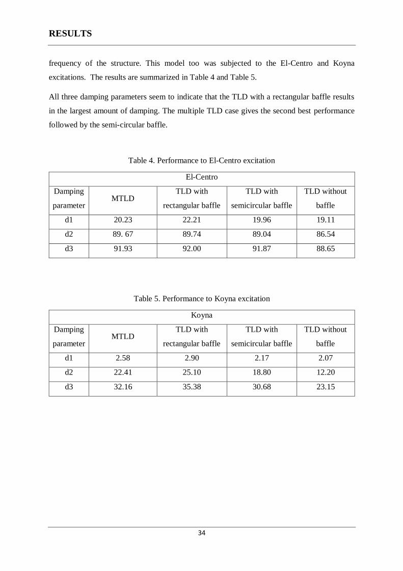
excitations. The results are summarized in Table 4 and Table 5.

All three damping parameters seem to indicate that the TLD with a rectangular baffle results

in the largest amount of damping. The multiple TLD case gives the second best performance

followed by the semi-circular baffle.

Table 4. Performance to El-Centro excitation

El-Centro

Damping

parameter MTLD

TLD with

rectangular baffle

TLD with

semicircular baffle

TLD without

baffle

d1 20.23 22.21 19.96 19.11

d2 89. 67 89.74 89.04 86.54

d3 91.93 92.00 91.87 88.65

Table 5. Performance to Koyna excitation

Koyna

Damping

parameter MTLD

TLD with

rectangular baffle

TLD with

semicircular baffle

TLD without

baffle

d1 2.58 2.90 2.17 2.07

d2 22.41 25.10 18.80 12.20

d3 32.16 35.38 30.68 23.15

35

7. CONCLUSIONS

This study, while confined to shallow water TLD was aimed at investigating the effect of mass

of fluid in the tank, devising parameters to measure the extent of damping and to explore

mechanisms for enhancing the performance of a TLD to a broad band excitation.

The parameters adapted to measure damping performed quite well for all the cases considered.

In all the cases, the damping parameters showed a very similar pattern: although their

magnitudes were different. Thus these parameters can be used to compare the extent of

damping for different configurations of the dampers in a numerical analyses.

The studies performed to establish the effect of mass of fluid on the damping resulted in some

interesting conclusions. The graphs describing the variation of the damping parameters with

frequency ratio illustrate that TLDs with comparatively small fluid mass seem to be more

effective over a wider frequency range than TLDs with a larger mass of fluid. While more

damping can be achieved with a TLD of higher mass when the frequency of excitation is close

to the tuned frequency, its performance will rapidly degrade when the frequency ratio is

substantially different from one.

The study also establishes the effectiveness of baffles in helping achieve better damping

performance for broad band frequency of excitation. Rectangular baffles seem to be more

effective than semicircular baffles with radius equivalent to the height of the rectangular baffle.

A Fast Fourier Transform of the response shows that a TLD with rectangular baffle has two

prominent frequencies of sloshing. The first frequency is the fundamental frequency of sloshing

due to the entire length of the tank, while the second peak is due to the length by which the

baffle divide the total length as explained in the previous sections.

Damping over a wider band of excitation can also be achieved by using several TLDS

(MTLDs) with different frequencies. However, the same effect can be achieved more

economically by using a single TLD with a baffle, since the fabrication and construction cost

of a baffle is likely to be considerably less than the cost of constructing multiple TLDs. Also

the present results seem to indicate that the performance of TLDs with rectangular baffles may

be superior to that of multiple TLDs.

36

8. REFERENCES

[1] ABAQUS 6.9 Benchmarks Manual..

[2] ABAQUS 6.9 User Manual.

[3] Banerji P. ,"Tuned Liquid Dampers for Control of Earthwuake response,",paper presented at

Thirteenth World Conference on Earthquake Engineering,Vancouver,B.C., Canada,August 1-

6,2004.

[4] Biswal KC, Bhattacharya S.K. and Sinha P.K., "Dynamic response analysis of a liquid-filled

cylindrical tank with annular baffle," Journal of Sound and Vibration, vol. 274, pp. 13-37, 2004.

[5] Chakrabarti S.K., Hydrodynamics of Offshore Structures, Southampton Bosto: Computational

Mechanics Publications, 1994.

[6] Dorothy Reed, Harry Yeh and Jinkyu Yu, "Investigation of Tuned Liquid Damperd under large

amplitude of excitation," Journal of Engineering Mechanics, vol. 10, pp. 1082-1088, 1996.

[7] Dorothy Reed, Harry Yeh, Jinkyu Yu and Sigur Gasdsson, "An Investigation of Tuned Liquid

dampers for Structural Control". Kareem, Yalla and McCullough, "Sloshing-Slamming Dynamics-

S2-Analogy for Tuned Liquid dampers," Vibro-Impact Dynamics of Ocean Systems, vol. 44, pp.

123-133, 2009.

[8] Jin-Kyu-Yu, Toshihiro Wakahara and Dorothy A. Reed, "A Non-Linear Numerical Model of the

Tuned Liquid Damper," Earthquake Engineering and Structural Dynamics, vol. 28, pp. 671-686,

1999.

[9] Kareem, Yalla and McCullough, "Sloshing-Slamming Dynamics-S2-Analogy for Tuned Liquid

dampers," Vibro-Impact Dynamics of Ocean Systems, vol. 44, pp. 123-133, 2009.

[10] Kondo I. and Hamamoto T. ,"Seismic Damage Detection of Multi-Story Buildings Using

Vibration Monitoring,". Paper presented at Eleventh World Conference on Earthquake

Engineering,1996 (paper number 988).

[11] Modi V.J. and Akinturk A., “An efficient liquid sloshing damper for control of wind-induced

instabilities”, Journal of Wind Engineering and Industrial Aerodynamics,vol. 90, pp. 1907-1918,

2002.

[12] Modi V.J. and Munshi S.R., “AN EFFICIENT LIQUID SLOSHING DAMPER FOR VIBRATIONAL

CONTROL”, Journal of Fluids and Structures, vol. 12, pp. 1055-1071, 1998.

[13] Nakayama and Washizu, "The boundary element method applied to the analysis of two-

dimensional non-linear sloshing problems," International Journal of Numerical Methods in

Engineering, vol. 17, pp. 1631-1646, 1981.

[14] R. A. Irahim, Liquid Sloshing Dynamics Theory and Applications, New York, USA: Cambridge

University Press, 2005.

37

[15] Yamamoto K. and Kawahawa M.,”Structural Oscillation Control using Tuned Liquid Damper”,

Computers and Structures,vol. 71, pp. 435-446,1999.

numerical analysis of tuned liquid dampers - kamalendu ghosh (09ce3112)

Documents

structural engineering

degree of master

great pleasure

partial fulfillment

great deal of indebtedness

project work

numerical study

kamalendu ghosh 09ce3112