numerical and analytical solutions to benchmark …numerical and analytical solutions to benchmark...

AD-A269 351lll~~iiL~lill11111 !l!11111 11111 ll~l4'1+

Defense Nuclear Agency UAlexandria, VA 22310-3398

DNA-TR-92-176

Numerical and Analytical Solutions to BenchmarkProblems Related to Tunnel Mechanics

Donald A. Simons TICLogicon R & D Associates E*LSEP -u9P.O. Box 92500 S 4Los Angeles, CA 90009

September 1993

Technical Report

CONTRACT No. DNA 001-88-C-0046

Approved for public release;distribution Is unlimited.

93-212350• 9 °0 00 0l0ll

p

Destroy this report when it is no longer needed. Do notreturn to sender.

PLEASE NOTIFY THE DEFENSE NUCLEAR AGENCY,ATTN: CSTI, 6801 TELEGRAPH ROAD, ALEXANDRIA, VA

22310-3398, IF YOUR ADDRESS IS INCORRECT, IF YOUWISH IT DELETED FROM THE DISTRIBUTION LIST, ORiFTHEADDRESSEE IS NO LONGER EMPLOYED BYYOUR

ORGANIZATION.

°ON4"

• p

p

• • •• • • • " "4

REPORT DOCUMENTATION PAGE M No. ov- 0 18 8

P @Wlc repan bwdft or * coledliaon of ,nblan Is .efeV tO a1 o l horw Per r• fpot *d•i re *m for rewetwfig rk swo. sw" ewmtn data soteO.g9rwk uo mfk*rg ft dat ne"ded, ad ownp• g d r&W lewk ft ocledlor of irdnw Sen ownmenb regadin VU brden oaefale or wr otrw aspet of 1146•Sedian of invomo.,dki Inuding emuggeei' for mwddng C. bum, *to WIDtVngtn Hafte Servkca Dlrec for Infonn OWr0 a• d Repont. 121 JewmD"i H4wW. SOL& 1-04. AuIgon. VA 2 4302. a.d to "he Oc of Mapgnt ad Budget Peev R"don fPto (070"1 W). Wa ,On. DC2060

1. AGENCY USE ONLY C save blank) 2. REPORT DATE 3. REPORT TYPE AND DATES COVERED

1930901 ITechnical 910401 - 9209154. TITLE AND SUBTITLE 5. FUNDING NUMBERS

Numerical and Analytical Solutions to Benchmark Problems Related to C - DNA 001-88-C-0046Tunnel Mechanics PE - 62715H

6. AUTHOR(S) PR -RDTA -RC

Donald A. Simons WU - DH000015

7. PERFORMING ORGANIZATION NAME(S) AND ADDRESS(ES) 8. PERFORMING ORGANIZATIONREPORT NUMBER

Logicon R & D Associates RDA-TR-2-2270-2402-001P.O. Box 92500Los Angeles, CA 90009

9. SPONSORING/MONITORING AGENCY NAME(S) AND ADDRESS(ES) 10. SPONSORING/MONITORINGAGENCY REPORT NUMBER

Defense Nuclear Agency6801 Telegraph Road DNA-TR-92-176Alexandria, VA 22310-3398SPSD/Senseny

11. SUPPLEMENTARY NOTES

This work was sponsored by the Defense Nuclear Agency under RDT&E RMC Code B4662D RD RC 0001525904D.

12a. DISTRIBUTION/AVAILABILITY STATEMENT 12b. DISTRIBUTION CODE

Approved for public release;distribution is unlimited.

13. ABSTRACT (Maximum 200 words)In this report, five numerical approaches to problems of tunnel dynamics are compared with each other and-wherever possible-with exact analytic solutions. The medium is an idealization of a jointed rock mass. Theintact rock is linear elastic-plastic with a pressure-dependent failure surface and associated plastic flow law.There arc two orthogonal sets of equally spaced joints. Each joint is nonlinear elastic in the normal directionand linear elastic with Coulomb friction in shear. All the methods but one represent the intact rock by continu-um elements; the other treats it as rigid and lumps its compliance in the joints. Most methods represent thejoints as sliding interfaces, but one models them also as finite elements. Most methods have two differenttypes of models for jointed rock, an explicit one where the joints are treated separately, and an implicit onewhere their properties are lumped together with those of the intact rock. Seven problems are posed. In thesimplest of the problems a strain history is specified for a block of intact rock. In the most complex, a linedtunnel in jointed rock mass is engulfed by a cylindrically divergent stress wave. A complete analytic solutionis derived for the first problem, incrementally analytic ones for the next four, and an idealized static orthotrop-ic elastic solution for the last one. Based on a combination of physical understanding (of wave propagationand material behavior) and comparison with the analytic solutions, three of the numerical approaches arejudged to have produced credible results to final problem.

14. SUBJECT TERMS 15. NUMBER OF PAGES

122Benchmark Tunnel Mechanics 16. PRICE CODETunnel Deformation Tunnel Vulnerability17. SECURITY CLASSIFICATION 18. SECURITY CLASSIFICATION 19, SECURITY CLASSIFICATION 20. LIMITATION OF ABSTRACTOF REPORTI OF THIS P)AGE OF ABSTRACT

UNCLASSIFIED UNCLASSIFIED UNCLASSIFIED SARNSN 7540-280-5500 Standard Form 298 (Rev.2-89)

Prnasobed by ANSI Sta. 2384182W8-02

• • •• • •• •

UNCLASSIIEDSECURITY C.ASSIFICATON OF TM PAGE

CLASSIFIED BY:

N/A since Unclassified.

DECLASSIFY ON:N/A since Unclassified.

SEC'13UY QASS!FICATION GWiTHIS VALE

UNCLASSIFTED

• -• • • • •

4PREFACE

This repoit was prepared at Logicon RDA as part of RDA's technical support to DNAunder the SETA contract (DNA001-88-C-0046). Paul Senseny (DNA/SPSD) served as technicalmonitor. The report relies hLavily on analysis performed by fotir contractors and a governmentlaboratory under DNA funding, also monitored by Dr. Senseny. The analyses by RE/SPEC wasperformed under subcontract to SwRl, and was monitored at SwRI by Ben Thacker. The analysisby Itasca was performed under subcontract to Weidlinger Associates.

The author would like to thank a number of other people for technical and editorialcontributions to this report. Above all, the benchmark study participants-Loren Lorig (Itasca),Francois Heuze and Ronald Shaffer (LLNL), John Osnes (RE/SPEC), Yoshio Muki and MarvinIto (CRT), and Felix Wong and Darrent Tennant (WA)-have been most helpful and willing tosupply information when asked. Those individuals and Da,,id Vaughan (WA) graciously wrotethe appendices describing their organizations' numerical approaches. Liz Garnholz (RDA)cheerfully digitized countless curves and prepared most of the figures. Eric Furbee (RDA)contributed some of the figures. Anita Gigliello and Kip Radler (RDA) helped with the finalpreparation of the document.

The numerical work by LLNL and the contractors was mainly performed betweenFebruary and July 1991, reviewed and discussed at three meetings during that same time span,and summarized in a series of briefing packages distributed at the time by RDA. The numericalresults reproduced here came for the most part from those briefing packages. The problemdefintionn and requested outputs had been spelled out in detail in a series of memos fromDr. Senseny and-in one case (problem 2-S)---by the author. In stveral cases some of therequested outputs were missing from one or more participant's presentat;oll. Except in oneinstance where a part of the package had been mislaid, the author c-hose tu work only with theavailable information. Thus when comparisons are presented among vairicus calculations, resultsmay be missing for a particular organization. The reason is that the results had not beensubmitted in ihe first place, although usually no specific remark to that effect will appear in thetext.

NTIS CRA.i

' U ,•. •G,, .ct~d ,-; [; !'. ,• _llJ • . .. .

SBy

nIiii

- I .:• 3D ,,y .O'.',I

"S-7 ... - .. .. 0

CONVERSION TABLE

Conversion factors for U.S. customary to metric. (SI) units of measurement

To Convert From To Multiply

angstom meters (in) 1.000 000 X E-10atmosphere (normal) kilo pascal (kPa) 1.013 25 X E+2

bar kilo pascal (kPa) L.M 000 X E+2barn meter2 (m2) 1.000 000 X E-28

British Thermal unit (thermochemical) joule (JM 1.054 350 X E+3calorie (thermochemicai) joule (JM 4.184 000

cal (tbermochLnicJll/cm2 megajoule/mn(MJ/m 2 ) 4.184 000 X E-2curie giga becquerel (GBqr 3.700 000 X E+Idegree (angle) radian (rad) 1.745 329 X E-2

degree Fahrenheit degree kelvin (KW t,-=(to" + 459.67)/ 1.8electron volt joule MI 1.602 19 X E-19erg joule (J} 1.000 000 X E-7

erg/second watt (WM 1.000 000 X E-7foot meter (m) 3.048 000 X E-1foot-pound-force joule (J) 1.355 818

gallon (U.S. liquid) meter3 tm3) 3.785 412 X E-3inch meter Wml 2.540 000 X E-2jerk joule J 1.000 000 X E+2joule/kilogr.Am (J/Kg) (radiation doseabsorbed? Gray (Gy) 1.000 000

kilotons terajoulea 4.183kip (1000 lbfl newton MN) 4.448 222 X E+3kjpltnch 2 (kal) kilo pascal (kPa) 6.A94 757 X E+3

ktap newton-second/m 2 (N-a/m 2) 1.000 000 X E+2micron meter Wma 1.000 000 X E-6

mil meter (mr) 2.540 000 X E-5mile (international) meter (m) 1.609 344 X E+3

ounce kilogram (kgl 2.834 952 X E-2pound-force (lbf avoirdupois) newton (Ml 4.448 222

pound-force inch newton-meter (N-m) 1 129 848 X E-lpound-force/inch newton/meter (N/m) 1.751 268 X E+2pound-force/foot 2 kilo pascal (kPal 4.788 026 X E--2pound-force/Inch2 (p,%) kilo pascal (kPa 6.894 757pound-mans |Ibm avoirdupois) kilogram Ikg) 4.535 924 X E-1portnd-mans-foot2 (moment of inertia kilogram-meter2 lkg-lm2) 4.214 O1l X E--2

pound-mass/foot3 kilogram/meter 3 (kg/m 3 ) 1.601 846 X E*Irad (radiation dose absorbed) Gray (Gy)" 1.000 000 X E-2roentgen coulomb/kilogram (C/kg) 2.579 760 X E-4shake second (s) 1.000 000 X E-8

slug kilogram (kg} 1.4.59 390 X E+I

torr (mm Hg. 00CM kilo pascal (kPa) 1.333 22 X E-1

"The becquerel (Bql is the Sl unit of radioactivity: Bp = I eventla.

"•The Gray (Gy) is the SI unit of absorbed radiation.

iv

• • • •• 'D• "

TABLE OF CONTENTS

.Section Page

PREFACE .................................................................... iiiCONVERSION TABLE ........................................................ ivFIGURES .................................................................... viiiTABLES ............................................................ x

1 INTRODUCTION ............................................. 11.1 BACKGROUND AND OBJECTIVE ............................ 1

1.2 SCOPE ................................................ 2

2 GENERAL SPECIFICATIONS ..................................... 4

2.1 GEOMETRY ............................................ 42.2 MATERIAL MODELS ..................................... 4

3 STATEMENTS AND RESULTS 1OR PROBLEMS WITHANALYTICAL SOLUTIONS ..................................... 7

3.1 ANALYTIC TREATMENT OF MATERIAL RESPONSE ............. 73.2 PROBLEM 1-IN: SPHERICALLY DIVERGENT STRAIN PATH

IN INTACT ROCK ....................................... 9

3.2.1 Statement of the Problem ............................... 93.2.2 Analytic Solution ................................... 103.2.3 Numerical Solutions ................................. 12

3.3 PROBLEM 1-IM: SPHERICALLY DIVERGENT STRAIN PATHIN IMPLICITLY JOINTED ROCK ........................... 14

3.3.1 Statement of the Preblem .............................. 143.3.2 Analytic So!ution ................................... 143.3.3 Numerical Solutions ................................. 16

3.4 PROBLEMS 2-EX AND 2-IM: UNIAXIAL STRAIN OF A"9STACK OF BRICKS1 . . . . . . . . . . . . . . . . . . . . . . . . . . . . . . . . . . . 16

3.4.1 Statemcnt of the Problem .............................. 163.4.2 Analytical Solution .................................. 193.4.3 Numerical Solutions ................................. 19

3.5 PROBLEM 2-S: SHEAR1NC7 OF TWO TRIANGULAR BLOCKSSEPARATED BY A SINGLE JOINT ......................... 22

V

• € q • •• • • ,. "

TABLE OF CONTENTS (Continued)

Section Page

3.5.1 Statement of the Problem .............................. 223.5.2 Analytical Solution .................................. 233.5.3 Analytical and Numerical Results ........................ 293.5.4 Why PRONTO Was Not Applicable to Problem 2-S ........... 33

4 PROBLEM STATEMENTS AND RESULTS FOR TWO-DIMENSIONAL PROBLEMS ................................... 34

4.1 PRELIMINARY DISCUSSION .............................. 344.2 PROBLEM 3: DIVERGENT WAVE PROPAGATION THROUGH

A JOINTED ROCK ISLAND ............................... 34

4.2.1 Statement of the Problem .............................. 344.2.2 Physical Effects Observed in the Numerical

Solution ......................................... 364.2.3 Numerical Issues .................................... 42

4.3 PROBLEM 4: LINED TUNNEL IN A JOINTED ROCK ISLANDSUBJECTED TO DIVERGENT WAVE PROPAGATION .......... 44

4.3.1 Statement of the Problem .............................. 444.3.2 Physical Effects Observed in the Numerical

Solutions ........................................ 454.3.3 Orthotropic Elastic Predictions of Stresses .................. 564.3.4 Remarks on the Numerical Solutions to Problem 4 ............ 59

5 CONCLUSIONS .............................................. 61

6 REFERENCES ............................................... 63

Appendix

A DESCRIPTION OF THE PRONTO2D COMPUTER CODE USEDIN THE UNDERGROUND TECHNOLOGY PROGRAMBENCHMARK ACTIVITY ..................................... A-1

B THEORETICAL ASPECTS OF THE LLNL DIBS DISCRETEELEMENT CODE USED IN THE DNA/UTP BENCHMARKEXERCISE ................................................ B-1

AIvi

• • •• • •• •

0 0,00

TABLE OF CONTENTS (Continued)

Section Page

C DESCRIPTION OF FINITE ELEMENT METHOD USED IN UTPBENCHMARK ACTIVITY BY CALIFORNIA RESEARCH ANDTECHNOLOGY ............................................. C-1

D DESCRIPTION OF THE DISTINCT ELEMENT METHOD USED INTHE UNDERGROUND TECHNOLOGY PROGRAM (UTP)BENCHMARK ACTIVITY ..................................... D-1

E THE APPLICATION OF THE FLEX PROGRAM TO UTPBENCHMARK PROBLEMS .................................... E-1

vii

L a-7

FIGURES

Figure Page

3-1 Geometry and loading in problems 1-IN and 1-IM .................. 93-2 Intact rock compressibility in problem 1-IN ...................... 133-3 Intact rock stress path in problem 1-IN ......................... 133-4 Implicitly jointed rock compressibility in Problem 1-IM .............. 173-5 Implicitly jointed rock stress difference vs pressure in

problem 1-IM .......................................... 173-6 Implicitly jointed rock effective stress (J2')12 vs pressure in

problem 1-IM ......................................... 183-7 Geometry and loading in problems 2-EX and 2-IM ................. 183-8 Jointed rock compressibility in problem 2-EX ..................... 203-9 Stress path in problem 2-EX ................................. 203-10 Compressiblity in problem 2-IM .............................. 213-11 Stress path in problem 2-IM ................................. 213-12 Geometry and loading in problem 2-S .......................... 223-13 Decomposition of joint displacements .......................... 263-14 Overall compressibility in problem 2-S ......................... 303-15 Von Mises effective stress path in problem 2-S .................... 313-16 Joint shear displacement vs shear stress in problem 2-S .............. 313-17 History of deformation mode in problem 2-S ..................... 324-1 Geometry and loading in problem 3 ........................... 354-2 Radial stress at tunnel location in problem 3 ...................... 364-3 Radial velocity at tunnel location in problem 3 .................... 374-4 Strain path at 500-m range, 2 degrees off axis, in

problem 3 ............................................ 384-5 On-axis strain paths in implicitly jointed and intact rock,

analytic solution and Itasca calculation, problem 3 ................ 394-6 Stress path at 487-m range on axis in implicitly jointed

rock in problem 3 ...................................... 404-7 Compressibility at 487-m range on axis in problem 3 ............... 414-8 Radial stress pulse shapes at 480, 500, and 520-m ranges

in problem 3 .......................................... 424-9 Hoop stress at 512-m range on axis, implicit and explicit region,

problem 3 ............................................ 434-10 Geometry and loading in problem 4 ........................... 444-11 Crown-invert closure in problem 4 ............................ 454-12 Springline closure in problem 4 .............................. 464-13 Radial stress field near the tunnel at peak free field stress arrival

time (about 30 ms) ...................................... 484-14 Tangential stress field near the tunnel at peak free field stress

arrival time (about 30 ms) ................................. 49

viii

VII~oo

0 0 0 0 0 0 0 ', 0

FIGURES (Continued)

Figure Page

4-15 Radial stress field near the tunnel at the end of the free-fieldpositive phase (about 120 ms) .............................. 50

4-16 Tangential stress field near the tunnel at the end of the free-fieldpositive phase (about 120 ms) .............................. 51

4-17 Slip along horizontal joints at peak free-field stress arrival ............ 524-18 Slip along horizontal joints at the end of the free-field

positive phase .......................................... 534-19 Deformed tunnel shapes at end of positive phase (about 120 ms) ....... 55

ix

• t •• • •• • "

TABLES

Table Page

1-1 The UTP benchmark problems ................................ 21-2 Participants in the UTP benchmark calculational exercise .............. 32-1 Standardized geometric parameters ............................. 42-2 Material properties ........................................ 53-1 Analytic solution to problem 1-IN ............................. 113-2 Imposed boundary displacements in problem 2-S .................. .233-3 Potential deformation modes in problem 2-S ...................... 233-4 Road map for computational scheme used in problem 2-S ............ 254-1 Joint slip contribution to springline closure ....................... 54

x

0 9 0 0 0 0 0 0

SECTION 1

INTRODUCTION

1.1 BACKGROUND AND OBJECTIVE.

In 1989 the Defense Nuclear Agency (DNA) initiated the Underground TechnologyProgram (UTP), a multi-year investigation into the vulnerability of underground structures. Theprogram includes calculations, material modelling, laboratory testing, and field testing all aimedat improving the ability to predict the response and failure of underground structures subjectedto ground shock due to near-surface explosions. The emphasis is on deeply buried tunnels withlittle or no reinforcement. The focal point of the program is a field test to be conducted atFt. Knox, wherein a buried high-explosive charge wili be used to load various deeply buriedstructures in a saturated limestone formation.

During the course of the UTP at least five different organizations have been engaged innumerical modelling of various aspects of the relevant dynamic processes. Each organization hasits own preconceptions about how best to construct these models. In order to explore theinfluence of the particular computational approach on the outcome of the numerical simulation,DNA conducted a "benchmark calculation' exercise. Several idealized problems were. defined,and each participating organization was asked to apply its computational tools to generate certainspecified outputs. This report summarizes the results of that activity.

Large rock masses inevitably contain discontinuities which are referred to as joints. Inmany cases they occur in one or several parallel sets with individual joints spaced at regularintervals. The numerical treatment of the combined effect of motion across joints anddeformation of the intervening conitinisous blocks poses a formidable challenge. Most of theparticipants use two general, complementary approaches: explicit, in which the motions acrossthe joints and the deformations within the blocks are represented separately; and implicit, whereina single, effective medium is defined so as to deform on the average like an assemblage of blocksand joints1. An implicit model, once defined, can be (and was in this study) used just like anyother material model in a general purpose finite-element or finite difference code, while explicitmodels require special treatment. The model types are complementary in the sense that whenapplied to tunnel failure problems, the implicit models--which are more computationally efficient-suffice in regions remote from the tunnel, while the explicit ones-which are locally moreaccurate-must be used near the tunnel if the details of individual block motions are to becaptured. As expected, the approaches to joint modelling provided the most stark contrastsamong the participants.

1Jn this report the terms explicit and implicit will always refer to the method for representingjoints. They will not refer to the time integration scheme, except in the following sentence. Allparticipants used explicit time integration.

LI

1.2 SCOPE.

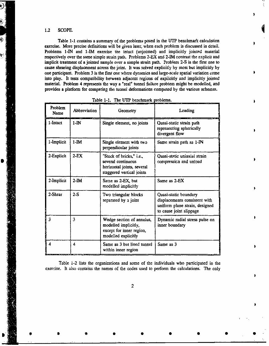
Table 1-1 contains a summary of the problems posed in the UTP benchmark calculationexercise. More precise definitions will be given later, when each problem is discussed in detail.Problems I-IN and 1-IM exercise the intact (unjointed) and implicitly jointed materialrespectively over the same simple strain path. Problems 2-EX and 2-IM contrast the explicit andimplicit treatment of a jointed sample over a simple strain path. IP1roblem 2-S is the first one tocause shearing displacement across the joint. It was solved explicitly by most but implicitly byone participant. Problem 3 is the first one where dynamics and large-scale spatial variation comeinto play. It tests compatibility between adjacent regions of expiicitly and implicitly jointedmaterial. Problem 4 represents the way a "real" tunnel failure problem might be modelled, andprovides a platform for comparing the tunnel deformations computed by the various schemes.

Table I-1. The UTP benchmark problems.

Problem Abbreviation Geometry LoadingName1

7

1-Intact 1-IN Single element, no joints Quasi-static strain pathrepresenting sphericallydivergent flow

1-Implicit 1-IM Single element with two Same strain path as 1-INperpendicular joints

2-Explicit 2-EX "Stack of bricks," i.e., Quasi-static uniaxial strainseveral continuous compressicn and unloadhorizontal joints, severalstaggered vertical joints

2-Implicit 2-IM Same as 2-EX, but Same as 2-EXmodelled implicitly

2-Shear 2-S Two triangular blocks Quasi-static boundaryseparated by 3 joint displacements consistent with

uniform plane strain, designedto cause joint slippage

30 3 Wedge section of annulus, Dynamic radial stress pulse on

modelled implicitly, inner boundaryexcept for inner region,modelled explicitly

4 4 Same as 3 but lined tunnel Same as 3within inner region

Table 1-2 lists the organizations and some of the individuals who participated in theexercise. It also contains the names of the codes used to perform the calculations. The only

2

• • •• • •• •

* S 00 0o

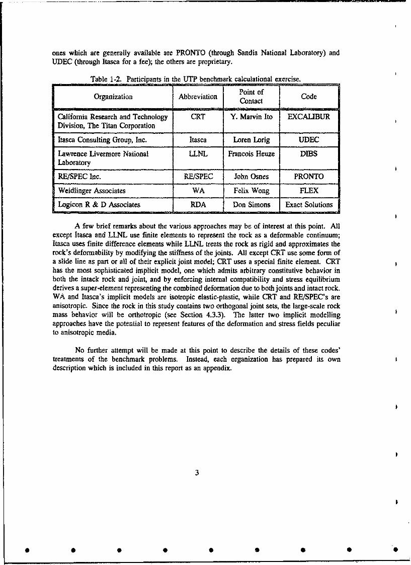
ones which are generally available are PRONTO (through Sandia National Laboratory) and

UDEC (through Itasca for a fee); the others are proprietary.

Table 1-2. Participants in the UTP benchmark calculational exercise.

Organization Abbreviation Point of CodeContact

California Research and Technology CRT Y. Marvin Ito EXCALIBUR

Division, The Titan Corporation

Itasca Consulting Group, Inc. Itasca Loren Long UDEC

Lawrence Livermore National LLNL Francois Heuze DIBSLaboratory

RE/SPEC Inc. RE/SPEC John Osnes PRONTO

Weidlinger Associates WA Felix Wong FLEX

Logicon R & D Associates RDA Don Simons Exact Solutions

A few brief remarks about the various approaches may be of interest at this point. Allexcept Itasca and LLNL use finite elements to represent the rock as a deformable continuum;Itasca uses finite difference elements while LLNL treats the rock as rigid and approximates therock's deformability by modifying the stiffness of the joints. All except CRT use some form ofa slide line as part or all of their explicit joint model; CRT uses a special finite element. CRThas the most sophisticated implicit model, one which admits arbitrary constitutive behavior inboth the intack rock and joint, and by enforcing internal compatibility and stress equilibriumderives a super-element representing the combined deformation due to both joints and intact rock.WA and Itasca's implicit models are isotropic elastic-plastic, while CRT and RE/SPEC's areanisotropic. Since the rock in this study contains two orthogonal joint sets, the large-scale rockmass behavior will be orthotropic (see Section 4.3.3). The latter two implicit modellingapproaches have the potential to represent features of the deformation and stress fields peculiarto anisotropic media.

No further attempt will be made at this point to describe the details of these codes'treatments of the benchmark problems. Instead, each organization has prepared its owndescription which is included in this report as an appendix.

3

SECTION 2

GENERAL SPECIFICATIONS

2.1 GEOMETRY.

For those problems involving joints (all except I-IN), a tunnel (4), or complexcomputational meshes (3 and 4), certain geometric parameters are standardized as shown inTable 2-1. Problems 3 and 4 are in plane strain, with a wedge-shaped mesh bounded by circulararcs of radii 450 and 550 m, a symmetry line through the tunnel location, and a ray at an angleof tan'1 0.1 = 5.71 (making the mesh 50 m wide at the tunnel location). An inner, rectangularregion extending 12.5 m in each direction from the tunnel location is modelled explicitly; therest, implicitly.

Table 2-1. Standardized geometric parameters.

. Dimension [Symbol Value

JitJoint Spacing S I mn

Joint Thickness 6 5 mm__ __ I JontSacn IS 5mm..

Range of Tunnel Ro 500 m

Tunnel Tunnel Diameter D 5 im

Liner Thickness T 50 mm

Cl Discrete Jointing Zone L 25 mMesh Mesh Height H 100 m

Mesh Divergence 0 tan" 0.1

2.2 MATERIAL MODELS.

The intact rock is treated as an isotropic, linear elastic and perfectly plastic material, withparameters summarized in Table 2-2. The plastic portion has an associated flow rule on a fixed(i.e., non-hardening) two-invariant stress surface fitted to a Mohr-Coulomb failure condition intriaxial compression. (This is sometimes called a Mises-Schleicher material.)

4

S- • = 0 0n•= - 0n - 1= • i n • umSummnnu 0m u n nn 0munu ~ aunnn Sum um•~n 1. .

Table 2-2. Material properties.

Property Symbol Value

Intact Mass Density p 2500 kg/m3

Intact Young's Modulus E 30 GPa

Intact Poisson's Ratio v 0.25

Intact Cohesion c 4.5 MPa

Intact Friction Angle 250

Intact Dilation Angle 250

Intact Tensile Strength T 2 MPa

Joint Normal Stiffness kN kN - 62 kPa/m

(6 -u,)2

Joint Shear Stiffness ks 1.25 GPa/m

Joint Cohesion c J 0

Joint Friction Angle 0 20°, except 300 in problem 2-S

Joint Dilation Angle I 0

Liner Young's Modulus EL 200 GPa

Liner Poisson's Ratio VL 0.30

liner Yield Strength CyL 400 MPa

Liner Mass Density PL 7500 kg/m3

To be more specific, the failure condition in terms of the principal stresses 01,02,03

(assumed positive in compression) can be written

f(olO2,o3) - 34/ - (a +bp)2 - 0 , (2-1)

2 222where 3J' - 01+02+03-0102-0203-130l and p - (01+02+03)/3 . When this is fitted toa Mohr-Coulomb failure criterion in a state of triaxial compression (o 2-oc3<ol) we find therelation between (ab) and (0,c) to be

a- 6ccos , b 6sin4o (2-2)a 3 _ sino b-3 - sin(

For the parameters given in Table 2-2 we have a=9.49 MPa, b=0.984.

5

This material specification is adopted for its computational simplicity. However, it isunphysical in that it leads to excessive dilatancy when compared with the response of real rocks.This needs to be kept in mind when assessing the results of problem 4, where-perhaps contraryto intuition, although not to certain lab and field observations-all calculators except one will beseen to predict that the tunnel suffers a decrease in the length of its springline (horizontaldiameter). The one exception-LLNL--did not model the rock as a continuum and consequentlycould not possibly represent its plastic response accurately.

The joint behavior is also assumed to bc clastic-plastic with a constant friction angle.However, the normal (opening/closing) elastic behavior is nonlinear, and the inelastic behavioris non-dilatant. The liner is elastic-perfectly plastic with a Mises failure condition and flow rule.Joint and liner property values are also listed in Table 2-2.

6

• • •• • •• •

0 0 0 n0 0 un .0n 0n 0a 0malammumnn • - .• == =. . = = n • u,• m nmm niuinunuuu u nnu__ _

ŽiCT1MON 3

STATEMENTS AND RESULTS FOR PROBLEMS WITH ANALYTICAL SOLUTIONS

3.1 ANALYTIC TREATMENT OF MATERIAL RESPONSE.

The first five problems (see Tab'e 1. 1) -re quasi-static ones driven by boundarydisplacements which are consistent with homogeneous (uniform) %train throughout the region ofinterest. This does not mean that the actual strains will be uniform.; if there are joints then actualstrains will not be uniform. But in fact the stresses and strairis in ýhe intzct rock and jointmaterial will separately be homogeneous at each point of the imposed strain path. This opensthe possibility of direct analytical solution of these problems for comparison with numeriralresults.

Another way of viewing the situation is that each of these probl'ms i-'cduces to nothingmore than finding the response of a single implicit elenicat around a specified strain path. Thisis strictly a material response question; equations of motion or compatibility among eiemernts playno role whatsoever. It is curious to note that only one of the participants (CRT) produced single-element solutions to all of the first five problems.

All five of these problems can easily be written in terms of principalstresses oaoo03 and strains E11,2 ,E3 . Also, in no case will any strain exceed three percent,so a small-strain analysis is sufficient. As usual, the strain increments are decomposed intcelastic and plastic parts

dE e - + d4P), (3-1)

with similar forms for da2 and dE3 . The elastic increments follow Hooke's law

df(e) - [tdoI -v(do2_do3] (3-2)

with similar forms for the other two components. The elastic response is easily invertible:E(1 -) [ .... (d dE

do1 - (1 -v) [d(e)+ ,(e) (e) (3-3)

If f(o 1,o2,o3 )<0, then the entire response is elastic and Eq. (3-3) fully describes the intact rockdeformation. Moreover, since the coefficients are constant, Eq. (3-3) can be integrated byinspection over any change in strain.

7

0 0 0 0 0 0 0 0 0O

U

The plastic increments follow from the associated flow law applied to the yieldfunction (2-1):

de = Xf=(34I -f Iay -Ao1-(o)+(7 3) -Y 1 (3-4)ao1

where X is a constant (to be determined) and similar formulas obtain for the other components.In (3-4) the constants a,,Py are given by

a = 2 P J+2b 22ab 3-5)99 -3

with (a,b) given by (2-2). When the intact rock is plastic, total strains are the sum of (3-2) and(3-4). An additional condition is that of continued yielding, which can either be written asEq. (2-1) or

df= "f d01+ Of d o2+ Of dq =0 , (3-6)001 Oo% 003

where the derivatives are given by formulas like the square-bracketed quantity in (3-4). Thethree principal stress increments can be found in terms of principal strain increments and currentstresses by solving the system of ten equations (3-1), (3-3), (3-4), (3-6) in the tenunknowns do1 , d), d4'P), X . We will defer this step until discussing specific problems.

It will be useful to represent the joint normal response in terms of stress. According toTable 2-2 the joint stiffness is

kN do Adk j- (6u)2 (3-7)

where A=625 kPa-in and uj = joint closure. This can be rearranged to give

A du,do =_ _

(6 -Uj) 2

This can easily be integrated, g;ving

CF Au.(6 -us)b

8

which can be inverted to give

620Uj = A+ub

The stiffness (3-7) can now be written in terms of stress:

kN =1I( , C) 2 (3-8)

3.2 PROBLEM 1-IN: SPHERICALLY DIVERGENT STRAIN PATH IN INTACT ROCK.

3.2.1 Statement of the Problem.

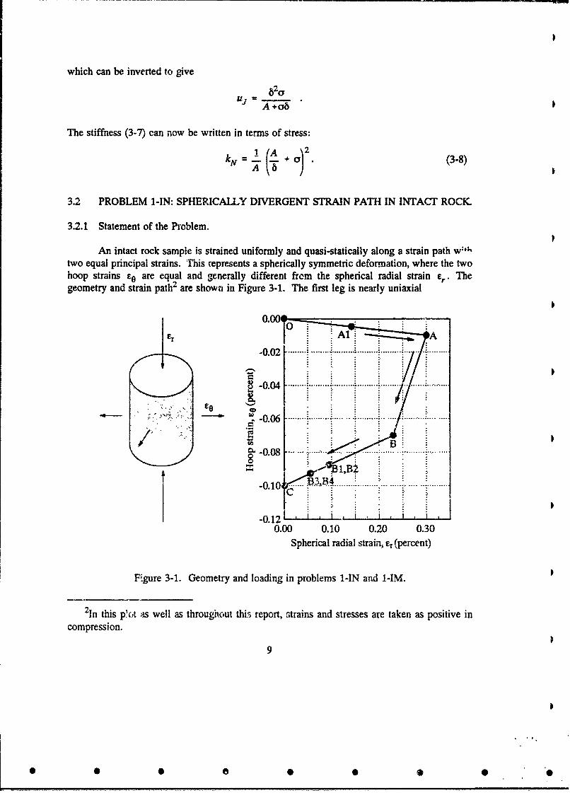
An intact rock sample is strained uniformly and quasi-statically along a strain path w:#;,two equal principal strains. This represents a spherically symmetric deformation, where the twohoop strains c9 are equal and generally different from the spherical radial strain F",. Thegeometry and strain path 2 are shown in Figure 3-1. The first leg is nearly uniaxial

-0.0-00 ......... ........ ..................... ...... .......... ....

S= -0.04 , ...-...,.. ..... 1 ................. ......... .. ......... i....

-0.00• •.......

0.00 0.10 0.20 0.30

Figure 3-1. Geometry and loading in problems 1-IN and I-IM.

21n this p'ot as well as throughout this report, strains and stresses are taken as positive in

compression.

9

• • •o • •• •

compression and represents the passage of a shock front. During thet second !eg, tensile hoopstrain accumulates due to outward radial displacement. In the third leg, the radial strain is fullyrelieved but a residual tensile hoop strain remains. The problem is to find the stresses at eachpoint along the given strain path.

3.2.2 Analytic Solution.

Let o1 0=r and 02=03=09 be the spherical radial and hoop stresses respectively, andsimilarly for strains. From (3-2), the elastic response is

S-1 (do, -2vd), [(1 -v)do o-vdor, (3-9)

with the inverse

d E[(1 -v)de) +2vdc0 )] E(dFs0e) +VdEr (3-10)doyr = r,0doe0=.(10 r3-)

(1 +v)(1-2v) (1+v)(1-2v)

In the elastic regime these equations govern the full response.

From (3-5) the plastic strain increments must obey

-r')=2X( _b)3 cprOI ') 0 -~pr= (3-11)

The differential form of the continuing yield condition (3-6) reduces to

(1 - b)dor-(1+2bld°de = 0 (3-12)

Equations (3-9), (3-11), and (3-12) combine with the two independent forms of (3-1) to provideseven linear equations in the unknowns (dE•), de(e), dc), dE), , or doo, X) . They can ber1 0 r 1 0solved for the stress increments during plastic loading, giving

dor = E(3 +2b)[(3 +2b) dar +2(3 -b) dE0 ]

27(1 -2v) +6b 2 (1 +v)

do0 = E(3 -b)[(3 +2b)der +2(3 -b)dc0 ] (3-13)

27(1 -2v) +6b 2(1 +v)

Note that with the given yield function and flow rule, not only the elastic formula (3-10)but the elastic-plastic one (3-13) as well are linear with constant coefficients. Thus as longas dEo/dEr is constant, the finite stress increments obey the same equations as the infinitesimals.

To compute the evolution of stresses along the strain path of Figure 3-1, we must proceedin steps, beginning with elastic response. On the initial leg OA we have d~o/dEr = -1/30

10

@ • @@ @ Q@ @

The stresses at any point along the leg are those at the beginning-O in this case-added to theincrements. Combining this strain increment ratio with (3-10) we find

Oe 30v-1 0.2954. (3-14)dor 30-32v

This holds until yielding, and in this case gives the ratio of stresses themselves since they bothstarted at 0. For this axisymmetric stress state the yield condition (2-1) can be recast

f = Ior-ol - •+b (2orr+Oo)] -0 (3-15)

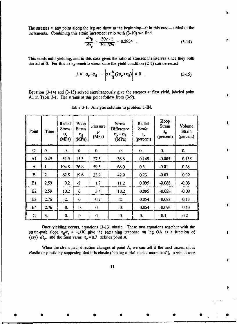
Equation (3-14) and (3-15) solved simultaneously give the stresses at first yield, labeled pointAl in Table 3-1. The strains at this point follow from (3-9).

Table 3-1. Analytic solution to problem 1-IN.

Radial Hoop pressure Stress Radial Hoop

Stress Stress Difference Strain Strain VolumePoint Time p GO Strain

oi, °0 (MPa) rpren) eret(MPa) (MPa) (MPa) (percent) (percent) (percent)

0 0. 0. 0. 0. 0. 0. 0. 0.

Al 0.49 51.9 15.3 27.5 36.6 0.148 -0.005 0.138

A 1. 104.8 26.8 59.5 68.0 0.3 -0.01 0.28

B 2. 62.5 19.6 33.9 42.9 0.23 -0.07 0.09

BI 2.59 9.2 -2. 1.7 11.2 0.095 -0.088 -0.08

B2 2.59 10.2 0. 3.4 10.2 0.095 -0.088 -0.08

B3 2.76 -2. 0. -0.7 -2. 0.054 -0.093 -0.13

134 2.76 0. 0. 0. 0. 0.054 -0.093 -0.13stanpt sl op oIj . 0. o. ! ___

LE__ 3. _ 0. 0. 0. 0. 0. -0.1 -0.2

Once yielding occurs, equations (3-13) obtain. These two equations together with thestrain-path slope E/E. -= -1/30 give the remaining response on leg OA as a function of(say) dEr, and the final value er = 0.3 defines point A.

When the strain path direction changes at point A, we can tell if the next increment iselastic or plastic by supposing that it is elastic ("taking a trial elastic increment"), in which case

11

• Q •• • •• •

from (3-10) with deo/dcr=6FI we find d0o/dor=31/33. With or>o0 and b=0.984 theincrement in the yield function (3-15) would be

df = d'r 2b - (3)1 ] b - 0.904do. (3-16)

With dor<O the trial increment would cause f to go positive, which is prohibited; therefore legAB must start with an elastic-plastic increment. Starting from the known state at A, as beforewe use (3-13) and the strain-path slope deo/d.r"=6/7 to find the changes in stresses as a functionof (say) der. Provided the tensile failure criterion is not met, the response will continue in theelastic-plastic mode until the next change in strain-path direction.

The tensile limit is given as 2 MPa, but no other details of the tensile failure law arespecified. In this analysis we assume this limit applies separately to each principal stress, andonce it is exceeded, that stress is set to zero.

Tensile failure therefore does not occur before reaching point B, so we can fill in the stateat B according to elastic-plastic response.

The beginning of leg BC is treated the same as was AB, and is likewise found to be,elastic-plastic. As before, the strain and stress increment ratios give the direction of the stresspath, and the starting point is known from the previous leg. The hoop stress is the first to reachthe tensile limit. Here the hoop stress changes abruptly from -2MPa (point B1) to 0 (point B2),while the radial strain remains fixed. The macroscopic hoop strain also stays fixed, but aftercracking, it will contain a portion due to the crack, while the intact material will contract in thehoop directions. Assuming the stress adjustments during crack formation are elastic, from (3-9),with dEr =-0 and do0 = +2 MPa we find dor =1 MPa. This completes the state at B2. (Ayield function check verifies that the stress adjustment was indeed elastic.)

The next leg is (as a trial) taken to be elastic, with o0= 0. Equation (3-9) thengiving dor-=-EdEr. Radial tensile failure occurs as or reaches -2 MPa at point B3. Now theradial stress also drops to 0 (point B4) with no change in macroscopic strain, and remains thereuntil the end of the strain path at point C.

3.2.3 Numerical Solutions.

The compressibility and stress paths from the various numerical solutions to problem 1-INare shown in Figures 3-2 and 3-3 respectively. The most obvious feature of these comparisonsis the inadequacy of the LLNL approach for representing stresses in intact rock. It has the wrongstiffness, volumetric hysteresis, and stress path over the full duration of the problem. Among theother curves. up to the point of tensile failure, all agree well except for slightly low unloadingpressures in the CRT model. The final leg of the compressibility curve suggests that all thenumerical models except RE/SFEC's used a criterion based on pressure rather than principalstress, and that after tensile failure some held the pressure at the cutoff value rather than fixingit at 0. Differences in intact rock tensile failure models are probably of negligible consequenceto tunnel failure in jointed media.

12

• • •• • QQ • "

60

CRT

RE/SPEC

40 LLNL : -,

WA . ,-

Itasca

L /o °

0I

-20 " . I ,-0.2 -0.1 0.0 0.1 0.2 0.3

Volumetric strain (percent)

Figure 3-2. Intact rock compressibility in problem 1-IN.

100

CRT - 780: / /:8 0. .... ... .... ... ... .. .. . . .. /-- -, ..... .. ........ ..... : ... .. ... .... .. ...... i.. .... .. ... ... ... ...... .. ... .

RE/SPEC /

WA /S 4 0 . .............. .......... ..................... !............... / .......... " .- ... ......... ... ...... '....................... ....

Itasca t /

S 2 0 ....t .... .. ... ... ..... . . ....................... ............................... ..

.exact0o ........ .. -.......... ......................... • ,... ....... ........ ..... ............................ !............................

.20 , I , I ,-40 -20 0 20 40 60

Pressure (MPa)

Figure 3-3. Intact rock stress path in problem 1-IN.

13

I

0 0 0 0 0 • 0 "0

3.3 PROBLEM 1-IM: SPHERICALLY DIVERGENT STRAIN PATH IN IMPLICITLYJOINTED ROCK.


The only difference between this problem and the previous one, problem 1-IN, is thematerial, which now contains two perpendicular joint sets modelled implicitly. One joint set isassumed to be normal to the r-direction (horizontal in Figure 3-1). Joint properties are given inTables 2-1 and 2-2.

3.3.2 Analytic Solution.

The introduction of impiicit jointing profoundly affects the solution in several ways: bycompounding the rock and joint response in each individual direction, by introducing nonlinearityon account of the joint's nonlinear normal stiffness, and by upsetting the axisymmetry on accountof the effective anisotropy induced by the joints. The principal stresses still align with coordinatedirections and joints, so there are still no shear stresses or shear displacements across joints, andit still suffices to consider only the normal stresses, strains, and displacements.

For this discussion, let the z-axis align with the r-direction and the normal to one jointset, and the x-axis with the other joint set. Consider the displacement increments for a singlejoint and intervening intact rock (i.e., a 1-m cube):

dd

dux = du + dux - w, dcx + xkx

du~ = du~ w (3-17)

duz ~du1 + du1 ze + Ldokz

where superscripts I, J refer to intact material and joints respectively, and w L- w, = w. = 1 m,The joint thickness has been neglected compared with the block width in relating intact rockstrains to the corresponding displacements. Recall that the joint stiffnesses kr , k. dependrespectively on the stresses ax , z according to (3-8). Combining (3-17) with the elasticconstitutive law (3-2) gives

14

• • Q• • •• • "

kV jdcN Edu, 38

sym m etric .. 11u,

Wz *J

This system of three linear equations must be solved simultaneously to get the elastic stressincrements corresponding to given displacement increments duX, duy, duz . The system as awhole is nonlinear, because the joint stiffnesses, and consequently the coefficients in (3-18),depcad on the current stress level.

Three of the equations governing stress increments in the plastic regime are found bycombining the elastic strain increments (3-2) with the plastic ones (3-4) and substituting the suminto (3-17). A ncw unknown X has been introduced, and the fourth and last required equationis the condition of continuing plastic yielding (3-6). The partial derivatives take the form of thesquare-bracketed quantity in (3-4). The resulting system of four equations in four unknowns is

_ -V -V E[aox-P(o+cF)-y] dl x

"+ Ed1 -v E[a a3 -l(X+o)-Y] 'oyt +--(319)

symmetric ... O

where in the axisymmetric problem at hand we have dux/wx duy/Wy= dee, dU z/Iwz -dEr .Note that the matrix in (3-19) is symmetric. This is a consequence of the associaited plastic flowlaw.

Either system (3-18) or (3-19) could be inverted in closed form if desired. However, thestress dependence of the resulting expressions for the stress increments would render them verydifficult if not impossibie to integrate in closed form. Therefore it was decided to perform boththe inversion and the integration numerically. The procedure for each time step is as follows:

15

• • •• • •• • I

jp(1) Solve the elastic equations (3-18), using current stresses, for trial stress increments

due to current displacement increments. Note that overall strain increments in theproblem specification (Figure 3-1), when applied to the 1-m cube, are numericallyequal to the displacements in meters appearing on the right-hand sides ofequations (3-18) or (3-19). A crude predictor-corrector is effected by updating thestresses and then re-solving the equations.

(2) Check whether the yield criterion is violated by the current stresses augmented bythe trial increments. If not, the current increment is elastic and the computed trialvalues are retained as actual values.

(3) it the current state is elastic but the trial values violate the yield criterion, linearlyinterpolate back to the p'ace where fO0. reset the time axis to this point, and moveforward from there with a plastic increment based on equxations (3-19).

(4) If the current state is plastic, first conduct an elastic trial as above. If the trial stateis elastic, update immediately (no interpolation is needed); if not, compute aplastic increment from (3-19) and update immediately.

It was not deemed of sufficient interest to pursue this computation beyond tensile failure,so it was simply terminated when any principal stress reached the tensile limit. The results aregiven with the numerical solutions in the following section.


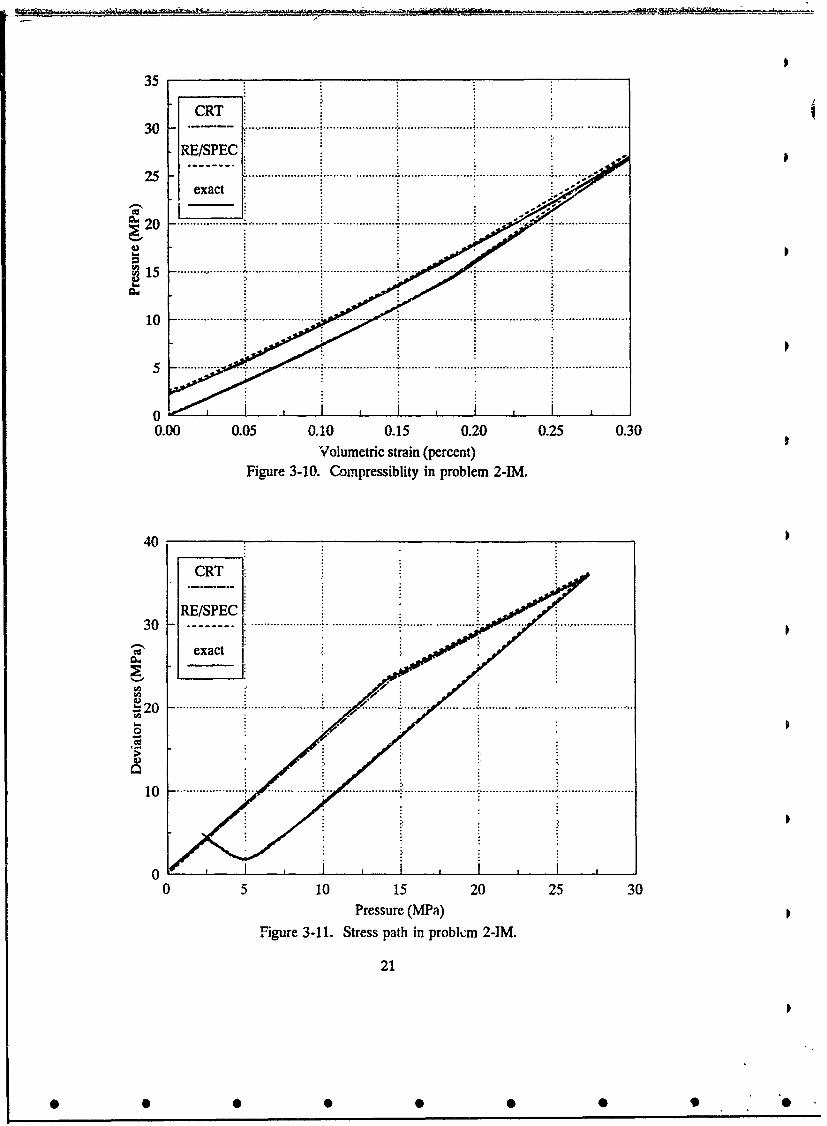
Only CRT and RE/SPEC submitted numerical solutions to this problem. Because it is notaxisymmetric, the stress difference o -o, is not equal to (3J2)lf2 , so three plots of resultsare given. Figures (3-4), (3-5), and (3-6) indicate that prior to tensile failure, both numericalresults are quite close to the analytical one. After that, altnough the analytic solution has notbeen carried this far, CRT's compressibility curve cannot be correct, since it does not terminateat a volumetric strain of -0.2 percent. However, as noted, this portion of the curve is not ofparticular interest in this problem.

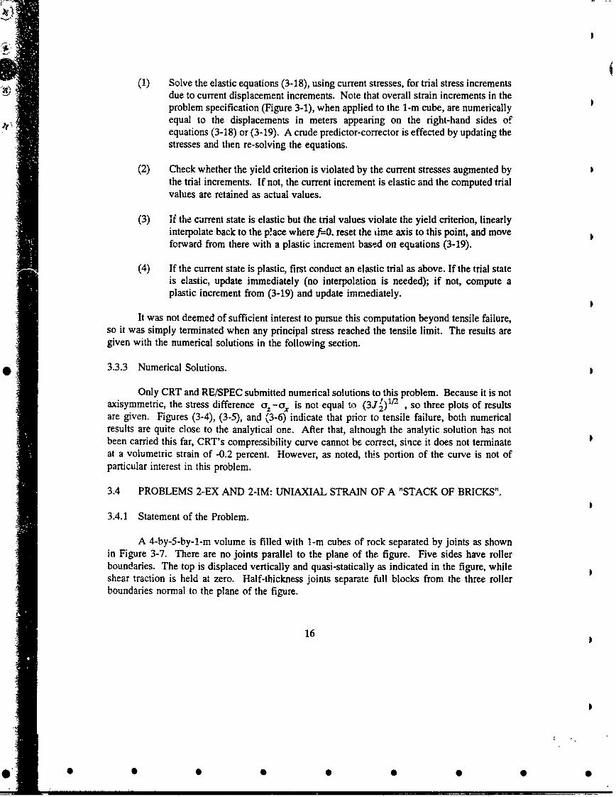
3.4 PROBLEMS 2-EX AND 2-IM: UNIAXIAL STRAIN OF A "STACK OF BRICKS".


A 4-by-5-by-l-m volume is filled with 1-m cubes of rock separated by joints as shownin Figure 3-7. There are no joints parallel to the plane of the figure. Five sides have rollerboundaries. The top is displaced vertically and quasi-statically as indicated in the figure, whileshear traction is held at zero. Half-thickness joints separate full blocks from the three rollerboundaries normal to the plane of the figure.

16

- = =

30

CRT

-RE/SPEC2 5 . . . ...... i......... .................. ........................... i.... ............... ... ....... ........... .. ..

20exact

10 ..........

-5

-0.2 -0.1 0.0 0.1 0.2 0.3Volumetric strain (percent)

Figure 3-4. Implicitly jointed rock compressibility in problem 1-IM.

40

exact

CIO

F-1

"• 10.."

-10 I i I Ii I

-5 0 5 10 15 20 25 30

Pressure (MPa)Figure 3-5. Implicitly jointed rock stress difference vs. pressure in problem 1-IM.

17

S• •0 0 0 0 0 0

40 :

CRT 1i.

30 RE/PEC

exact

1117.... ...

"iIS...... ....... . . ............

00v!

-10 ,, J , , , i ,

5 0 5 10 05 20 25 30Pressure (MPa)

Figure 3-6. Implicitly jointed rock effective stress (pr2'o1b vs. pressure in problem 14M.

S1.8

.04 ........... .0. ... .............. . .... .

0 .6 .... . . . . . .-....... . . . . . ............... .......

0 . ..-.- -. ...- --- ---- ..... ... .... .. .. ..

0.00.0 0.5 1.0 1.5 2.0

Note: Plane strain in third dimension Pseudo-time

Figure 3-7. Geometry and loading in problems 2-EX and 2-4M.

18

3.4.2 Analytical Solution.

No distinction between implicit and explicit rock models needs to be made for the purposeof deriving the analytic solution to this problem. The stated conditions lead to stresses andstrains identical to those in an infinite region with the same joint spacing and homogeneousmacroscopic strain. The principal directions of the geometry will coincide with principaldirections of stress and strain. Equations (3-18) and (3-19) from the previous section govern asingle, representative 1-m cubic element under these conditions. (The staggering in the jointingonly affects deformations at a much higher level of accuracy than considered here.) Therefore,the analytic solution to this problem follows exactly the same procedure as problem 1-IM. Theonly difference is the right-hand side of (3-18) or (3-19), where now du, = du = 0, and (fora single 1-m element) u, will increase quasistatically up to 0.3 cm and then decrease to zero.The results of the step-by-step numerical integration are shown in Figures 3-8 and 3-9.


Figures 3-8 and 3-9 also show the compressibility and stress path according to the variousexplicit numerical joint models. In each plot two curves stand out. The LLNL model again hasincorrect stiffness, hysteresis, and deviator stresses. It does appear to agree with the initial slopeof the compression loading curve, but not to stiffen on loading as it should due to the joint'snonlinear elastic compressive behavior.

The WA model has incorrect stiffness and excessive numerical chatter. The reason forthe former is that in the joint treatment used in this problem, joint stiffness was fixed solely bynumerical considerations related to the detection of and compensation for node penetration acrossjoints. There was no other mechanism to include a specified normal joint stiffness, so it wasignored. The required numerical stiffness appears to have been much greater than that specifiedfor the joint, leading to stiffer overall response. That the WA stiffness is roughly twice thecorrect value is consistent with the fact that at least according to specifications in the elasticregime, the contributions of the intact rock and joints to the overall stiffness are about equal.Subsequent to this calculation, the joint model was modified to admit a specified normal elasticstiffness in place of the former, numerically driven value.

The excessive chatter in both compressibility and stress path in the WA calculation is alsocaused by the joint model. WA explicitly modelled every individual block and interface shownin Figure 3-7. Subsequent to this problem, WA modified the treatment of joint forces at thecorners of blocks and believes that these modifications are responsible for the improvement inthe model's behavior in subsequent problems. (Appendix E contains a brief description of themodelling approach and the modifications.)

Numerical results for problem 2-IM are shown in Figures 3-10 and 3-11 together with theanalytical solution. Again, only CRT and RE/SPEC submitted solutions based on implicit jointmodels, and both agree closely with the analytical results.

19

• Q •• • •• •

60

CRT

50RB/SPEC s~.

40 L L N L .... ....... :............:..... ..... ..... ...........

0 30 . ..........

60

501

RE/SPEC/

'40 ....................

WA

oItasca

1 0 e. c ............ ..... .

0-10 0 10 20 30 40 50 b0 70

Pressure (MPa)Figure 3-9. Stress path in problem 2-EX.

20

0 0 0 000 00

35 .:.

CRT i

30 -L :,RE/SPEC

2 5 ....................... i ............. ......... ...................... ................... .. .. ..

exact

_20 . ........................................................................ . . ..............

S15 ......................................... : . ..... ....... ...... ................ -. ........... .......

10 ..................... .-...................... .................... ..... ....... .........................5o ... ... .... ........... .......f.............. .. ....................... .. ..00.00 0.05 0.10 0.15 0.20 0.25 0.30


Figure 3-10. Compressiblity in problem 2-IM.

40CRT :i

RE/SPEC30 ....... .......... .................. . .. . ....... ..........

2 0 ...............

10 ". ............. .. .. . ... . .. ... ..... .... .... .. . ..... .... ... .... .... ...

00 5 10 15 20 25 30

Pressure (MPa)Figure 3-11. Stress path in problcm 2-IM.

21

• • •• • •• •

3.5 PROBLEM 2-S: SHEAiRING OF TWO TRIANGULAR BLOCKS SEPARATED BY A

SINGLE JOINT.


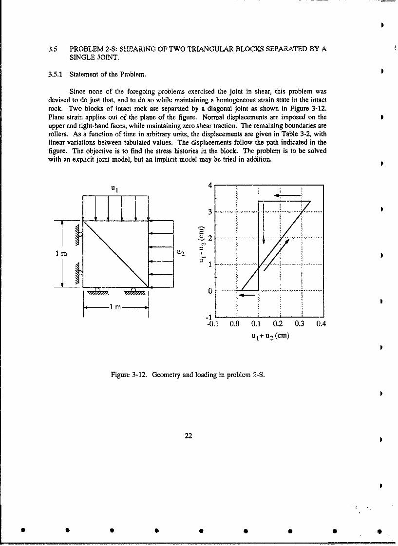
Since none of the foregoing problems exercised the joint in shear, this problem wasdevised to do just that, and to do so while maintaining a homogeneous strain state in the intactrock. Two blocks cf intaci rock are separated by a diagonal joint as shown in Figure 3-12.Plane strain applies out of the plane of the figure. Normal displacements are imposed on theupper and right-hand faces, while maintaining zero shear traction. The remaining boundaries arerollers. As a function of time in arbitrary units, the displacements are given in Table 3-2, withlinear variations between tabulated values. The displacements follow the path indicated in thefigure. The objective is to find the stress histories in the block. The problem is to be solvedwith an explicit joint model, but an implicit model may be tried in addition.

Ul 4

3 .......... .. .

2 ....... . . ..... ......

I &2 I1 m U: i ! i

-0.! 0.0 0.1 0.2 0.3 0.4

Ul+ u, (CM)

Figure 3-12. Geometry and loading in problem 2-S.

22

0I

Table 3-2. Imposed boundary displacements in problem 2-S.

Time(Arbitrary U1 U2

units) (m) (m)

0 0 0

1 0.0001 0.0001

2 0.0187 -0.0153

3 0.0175 -0.0165

4 0.0005 0.0005

5 0 0

3.5.2 Analytical Solution.

3.5.2.1 Outline of the solution procedure. The problem will be treated by anincrementally linear scheme. At the beginning of each time step the stresses, boundarydisplacements, total joint slip, and pending displacement increments are known, and the stressincrements and total joint slip increment are to be found. Once the increments are found, thecorresponding quantities are updated and the process repeated.

For quasi-static deformations, this problem can be put into the same form as the moreconventional one of elastic-plastic deformation with two intersecting, non-hardening failuresurfaces. One surface is the standard one for the intact material; the other is the locus in stress-space of points satisfying the conditions for Mohr-Coulomb frictional slip. Plastic flow in intactrock is associated, while the effective plastic strain due to joint slip is not associated with thejoint failure function. Table 3-3 lists the four potential deformation modes, and assigns a nameand number to each.

Table 3-3. Potential deformation modes in problem 2-S.

Mode number Mode name Intact responseI Joint response

1 EE Elastic Elastic (not slipping)

2 EP Elastic Plastic (slipping)

3 PE Plastic Elastic

4 PP Plastic Plastic

23

0 0 0 0 0 0 0 0 0

For each potential mode, a corresponding set of stress increments can always be obtained.The formulas will be given below. If the problem is well-posed, then one and only one of thesefour sets will be admissible, because together they comprise all of the possibilities. The criteriafor admissibility are that the stresses at the end of the increment be inside or on the appropriatefailure surface~s), and that the plastic strain increments for the active plastic mode(s) be in thecorrect direction. The former requirement is equivalent to the negativity or vanishing of thefailure function f 1 or fJ. For the intact rock, the latter requirement is that the proportionalityconstant X! relating plastic strain increments to stress derivatives of the flow potential, bepositive. For the joint, the condition is that the increment of slip must be in the same directionas the total shear stress across the joint. While no analytical proof of uniqueness is available,it will be found numerically for the prescribed boundary displacement history that at every timestep there is one and only one admissible solution among the four alternatives.

The computational procedure for each time step will begin with the evaluation of anumber of "trial" increments, the number and type depending on the location of the stress pointat the start of the increment. 3 Specifically, only increments of types which cannot be ruled outa priori, based on the starting point, will be considered. For example, if the starting point is EE,i.e., both failure functions are negative and the stress point is inside both failure surfaces, thenonly an EE increment need be considered. If starting with an EP stress state, where the stresspoint is on the joint failure surface but inside the one for intact material, the increment must beeither EP or EE. If a trial increment causes the stress point to cross a failure surface, then linearinterpolation is used to shorten the current time step such that the stress point will be right onthe failure surface at the end of the time step. This ensures that only a single deformation modeoccurs during the entire time step.

Table 3-4 is a road map of the entire computational scheme. The second column lists thetypes of trial increments that cannot be ruled out a priori for each starting stress point location(column 1) and are therefore computed and checked for admissibility. Conditions foradmissibility are listed in the third column in terms of failure functions and plastic flowproportionality constants. (Although we will not explicitly write the joint slip increment in theform of a constant multiplying the gradient of a flow potential, it could be done. In the table," V.J* > 0 " is simply shorthand for "the slip increment is in the same direction as the total shearstress across the joint.") The superscript "*" refers to a trial value, so forexample ft, =fJ(o+do*) where a is the stress at the start of the time step and do* is thetrial stress increment. The fourth column indicates the final resolution for the time step, basedon which pair of admissibility conditions holds. In some cases the trial increment itself becomesthe actual stress increment. In others, where the trial increment caused the stress point to crossa failure surface, an interpolation based on failure function values is applied to scale back boththe stress increment and the time step such that the end point is just on the failure surface(s).

3These "trial" increments should not be confused with the trial elastic increment used in mostexplicit dynamic codes.

24

• • •• • •• •

Table 3-4. Road map for computational scheme used in problem 2-S.

Stress state at Trial increment Admissible Action if Stress statestart of time types outcomes (see condition in at end ofstep note A) column 3 holds time step

EE EE f 1*<O, f*<O do--do" EEf1 *<O, fj*>O do=-•do EP

f*>O, f4*<O do=f?/do" PE

fr>O, f J*>0 (See note B) EP or PE

EP EE f*<O, f*<O do---do" EE

__ >Of'<o da- 1do" PE

EP f*<O, ?*>O do--do* EP

f'*>O, k'*>O do=fda* PP

PE EE fl*<O, fJ*<o do=do EE

f'<O, f4>O da=o/do" EP

PE W'>O, f'e<O do--do" PE

_ _">O, fj1 >O do=O/do" PP

PP EE fI*<o, fl*<O do--do" EE

EP ft*<O, A!*>O do--do" EP

PE x0>0O, f-*<O da=do" PE

I JIPP W1">0, kJ>0 doy--ao PP

Note A: For uniqueness, only one of the four conditions will hold.

Note B: This condition, corresponding to an EE starting point very near theintersection and a strain increment outside both surfaces, never occurred butcould be handled if necessary.

25

• • •• • •• • "

For example, the constant 01 , which must fall in the range (0,1), is defined by

f 1(c +do ) -fl(3)

Finally, the last column shows the location of the stress point at the end of the time step.

3.5.2.2 Analytical preliminaries. As before, we decompose the displacements into partsseparately due to intact material and the joint:

1 I I I

z = +z ="Z +; , =U =0 (0-20)

where the last relation expresses the plane strain condition in the uNJ,absence of any joints normal to the y-axis. As indicated by thevector diagram in Figure 3-13, the parts of the total displacementdue to motion across the joint can be further decomposed into Uzicomponents normal and tan gential to the joint. These arerespectively denoted uN (positive in compression)and us (positive when the upper block moves down and to the

right), and are given by UXJ

J J J J- UN US I u N -- (3-21) Figure 3-13. DecompositionSF2 of joint displacements

The symmetries of this problem guarantee that the only nonvanishing stresses in the x-y-zcoordinate system are the normal stresses in the coordinate directions. By a 45-degree cwcoordinate rotation, these give rise to the following normal and shear stresses across the joint:

O Oz + °x - Oi 0 z-Ox A(ON = 2 o 9 = - (3-22)2 '2 2'

In view of the form of (3-22) and other factors that lead to later simplification, we willregard the fundamental stress unknowns to be 5, Au, o. , and will seek equations for theincrements in these quantities in terms increments in the correspondingly defined quantitiesuAu, uy(=O).

26

0 0 0 0 0 0 0 0 "0

In preparation for that, by combining equations (3-7), (3-8), (3-21), and (3-22), the jointresponse law can be written in the form

J J J Jedu + dux+ duN, du

2

dAu .du- dux = V~du V2+(dm +ddiP) dAo + 3w• 2i (33Z S S S ~~F2ks S (-3

EI

kN= uA

where a superscript p denotes the contribution of "plastic" or slipping joint behavior. Similarly,by using equations (3-2), (3-4)e and (3-22)i the intact material response can be written

du I+ dux

2

( 1-v)da -vdc - -W E Y W~5Po+CY-1 (-4

dAu1 I duz - dux' = dAu + dAu 1P = w' EdAo + 3WXA!A

duy dule d'yP -2v da- doY.+W [c -2Z-y=0

If the intact material is in the elastic regime, equations (3-24) still obtain, but with ~!0

In the next four subsections we will combine and solve these equations for each possiblemode of deformation as summarized in Table 3-3. Once the four types of solutions are derived,they are used as the basis of a computer program which implements the logic embodied inTable 3-4.

3.5.2.3 Solution for mode 1 CEE) increments. For mode 1 (purely elastic response),equations (3-23) with vanishing joint slip increment (dUJ' =0 )and (3-24) with no intact rockplasticity ( 2=0 ) combine to give

27

dE du dAu- _ _ _ _ _ , dAo = _ __ _

1-v- 2V2 1 +vE F2kN E F2ks (3-25)

do., - 2vdo- , du dAo

Note that in mode 1 the increment in joint shear displacement dUsj is explicitly determined bythe joint constitutive law through the shear stiffness ks.

3.5.2.4 Solution for mode 2 LEP)P increments. For mode 2 there is still no intact rockplasticity (X, 0) but now the joint is slipping (du4P i 0) . The joint constitutive law nolonger explicitly governs the incremental shear stress-shear displacement across the joint.Instead, the Coulomb friction law relates the shear and normal stress across the joint:

Pf- J2 J2

(Ys) -( OA') - 0, (3-26)

where the coefficient of friction is related to the friction angle by 1i - tan C. The overallresponse equations analogous to (3-25) follow from (3-23), (3-24), and (3-26):

do - , dAo - sgn(Ao)2,d•y1 -v - 2v2 1

W_ +E F2"kN (3-27)

do, -2vdo- , duJ-I'(d,&u - W 1 Vd Acy S V72 E )

3.5.2.5 Solution for mode 3 (PE) increments. In mode 3, the plastic proportionalityconstant W! becomes an additional unknown. The first three equations governing the basicunknown increments are obtained as before by combining (3-23) and (3-24), but nowwith V # 0 . An additional equation comes from the condition of continued yielding (3-6). Inmatrix form the equations are

28

• • 6i) • g •

1-v 1 0 wvaB-p(+a,)-,] dW + • 0 -W-ww[iy-A F y) nd uE •F2kN E

0 w lv+ 1 0 3wAo dAo dAuE 2 dks=

_2 0 1 aOy -2P5 -y ddy 0E E

,.[a•a - l( + ay) - y] 3A----y aory -2P5 - y 0 0.2

(3-28)

We have elected to solve this set numerically during each time step when required, rather thanexplicitly.

3.5.2.6 Solution for mode 4 (PP) increments. In mode 4 both the intact material and thejoint are failing. The fundamental unknowns are taken as the three stress increments, A! , andthe joint slip increment dup . The equations governing the stress increments follow as beforefrom (3-23) and (3-24). The fourth equation is the condition of continued intact material yielding(3-6). The fifth is the differential form of the joint failure condition (3-26), which was alreadyused for mode 2 and appears as the second of equations (3-27). When assembled into matrixform the equations are

1-v+ 1 V w[a00 0-(+Oy)- A 0 ,5 duE F2 kN E

o +v +1 3 dAo dAu0 w 1 +v 0 3wAcy r o ~

E + r2 ks

-2 0 1 acy, - 2P3i - y 0 cE E-

3Ao clXI~y 02-[acy - P3 (FY + cyy) - y] Ma acy - 2Pi - y 0 00

-2p sgn(Ac) 1 0 0 0 U 1 ' 0

(3-29)

3.5.3 Analytical and Numerical Results.

In addition to the analytic solution just outlined, complete solutions using explicit jointmodels were submitted by CRT, WA, and Itasca. A partial solution was completed by LLNL

29

• • •• • •• • "

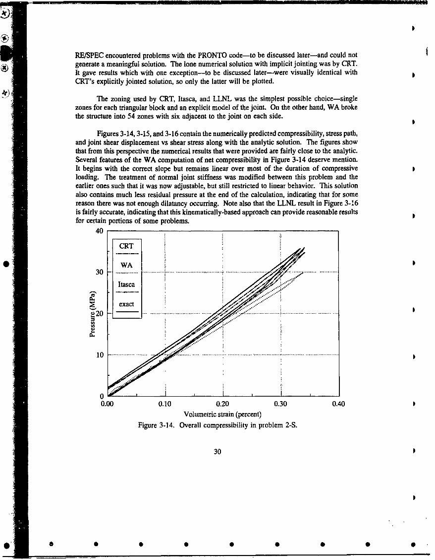
I

RE/SPEC encountered problems with the PRONTO code-to be discussed later-and could notgenerate a meaningful solution. The lone numerical solution with implicit jointing was by CRT.It gave results which with one exception-to be discussed later-were visually identical withCRT's explicitly jointed solution, so only the latter will be plotted.

The zoning used by CRT, Itasca, and LLNTL was the simplest possible choice-singlezones for each triangular block and an explicit model of the joint. On the other hand, WA brokethe structure into 54 zones with six adjacent to the joint on each side.

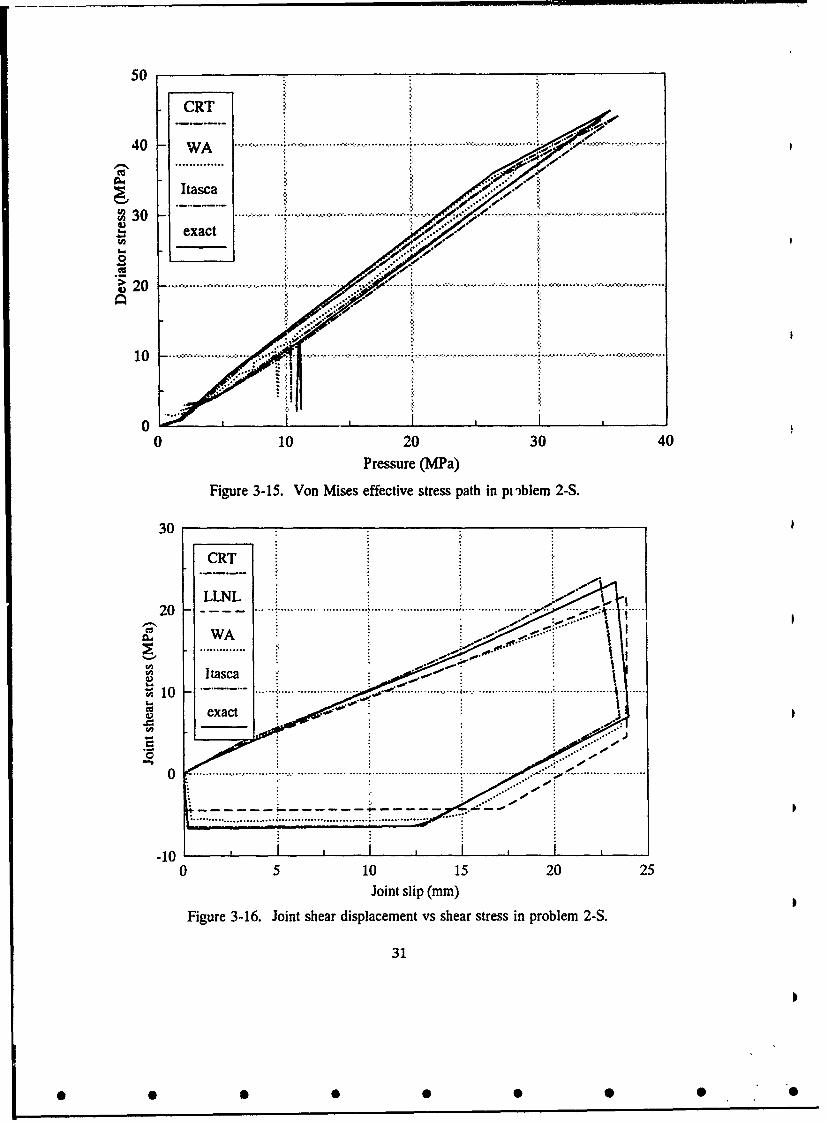
Figures 3-14, 3-15, and 3-16 contain the numerically predicted compressibility, stress path,and joint shear displacement vs shear stress along with the analytic solution. The figures showthat from this perspective the numerical results that were provided are fairly close to the analytic.Several features of the WA computation of net compressibility in Figure 3-14 deserve mention.It begins with the correct slope but remains linear over most of the duration of compressiveloading. The treatment of normal joint stiffness was modified between this problem and theearlier ones such that it was now adjustable, but still restricted to linear behavior. This solutionalso contains much less residual pressure at the end of the calculation, indicating that for somereason there was not enough dilatancy occurring. Note also that the LLNL result in Figure 3-16is fairly accurate, indicating that this kinematically-based approach can provide reasonable resultsfor certain portions of some problems.

40

CRT

@2 ~~WA .;3 0 . .............. .................... .................. ..... ... ......................... . . . . ..... .. ...... . .

Itasca

exact . -.

20.. .. ... ....... ............ .... V...............................

• ~."

10 ........... ............. ................................ .................

00.00 0.10 0.20 0.30 0.40


Figure 3-14. Overall compressibility in problem 2-S.

30

® • •• • •• •

50

CRT

40 W A ...... ..............

~I Itasca(030 ------

exact

0

20 ...

0 10 20 30 40Pressure (MPa)

Figure 3-15. Von Mises effective stress path in pi )blem 2-S.

30.

CRT

20L 02 0........ ................ ......... . ..

al

~ 10

0

-100 5 10 15 20 25

Joint slip (mm)

Figure 3-16. Joint shear displacement vs shear stress in problem 2-S.

31

Figure 3-17 shows the deformation mode vs time for those who provided this information.It is interesting to note that both CRT and Itasca predict a short episode of mode 4 (PP) responsestarting around t=1.8, while the analytic solution does not. This is where the CRT implicitsolution differs from explicit. The former stayed in mode 4 for only one time step, thus agreeingmost closely with the analytic one. From a practical standpoint, in this particular problem, thediscrepancy is of little significance; the stresses and strains in the four solutions are very closeto one another. However, this still raises some perplexing questions. On one hand, twoconscientious, meticulous calculators independently have reached the same result with theirexplicitly jointed models; on the other hand, the scheme detailed in Section 3.5.2, for numericallyevaluating the analytical solution, has been designed to probe all possible evolutionary paths fromeach stress point and to test each one for admissibility. At every stage, this scheme has identifieda unique admissible stress increment. In particular, in the analytic solution (and effectively inthe CRT implicit solution), the stress point approaches the intersection between the two failuresurfaces, moves right up to it (by interpolation), and then moves directly across it, while the twoexplicit numerical solutions predict a short traverse along the intersection. In the numericalscheme for the analytic solution, an increment along the intersection (mode 4 or PP) was one ofthe four which were explicitly tested for admissibility (see the last four rows of Table 3-3). It

analytic

4 (P) CRT

Itasca I4..

(P E ) . ......... ........................ ..... .. ... . ..... .... .......................

S2 (EP)

1 (E E ) .. .............. ...... ...... ...... .. . .....................

I I

0 1 2 3 4 5Pseudo-time

Figure 3-17. History of deformation mode in problem 2-S.

32

0 S 0 0 0 0 0 0 0

was found to lead to a joint slip increment opposite the prevailing shear stress across the joint,and so was deemed inadmissible. It is also interesting to note that the elastic trial incrementfrom this point gave rise to trial stresses which violated both failure conditions (and was ruledout for that reason). This is not the same as the elastic trial used by the numerical solutions4.Nevertheless, one might speculate that the numerically derived trial stresses in the explicit modelsalso violated both failure conditions and that this somehow initiated the excursion along theintersection of the failure surfaces. It may then have taken these methods a number of time stepsto recognize and correct for joint slippage opposite the shear stress across the joint.

3.5.4 Why PRONTO Was Not Applicable to Problem 2-S.

RE/SPEC elected always to treat the elastic properties of joints implicitly, i.e., bysmearing them out and distributing them in the surrounding intact material. Only the Coulombslip is represented explicitly. This may be reasonable if there are many such joints, but with justa single one it leads to difficulties when the joint is inclined. The problem stems from the factthat the RE/SPEC approach makes the surroundings behave like a transversely isotropic material,with the primary material axis aligned normal to the joint(s). In problem 2-S this axis is 45degrees from the geometric axes. To see the effect of this misalignment, consider the situationbefore any slippage occurs. The two triangular blocks are acting as a single, continuous squareone. Because of the anisotropy, the specified boundary conditions (constant normaldisplacements, vanishing shear traction) are not consistent with a homogeneous stress state withinthe block. In other words, with no shear traction the block would suffer a shear strain and wouldrequire linearly varying normal boundary displacements to maintain homogeneity; conversely,a particular value of shear traction could be applied which would cause shear strain to vanish.Therefore, when RE/SPEC set up and ran this problem with the specified boundary conditions,the stress state was nonuniform from the very beginning. Later the situation got even worse,because the joint failure condition was not met simultaneously all along the joint, not evenapproximately. Because the nonuniformities were traceable to particular features of the RE/SPECapproach in a way that was not anticipated when the problem was defined, it was decided notto pursue the solution to its conclusion with this method.

4For this problem, the trial elastic stresses used in the numerical solutions come from strainswithin each element which depend in part on internal (non-forced) nodal displacements, projectedfrom the previous time step by forward differences based on the momentum balace equations.

33

0 0 S S 0 5 0 0 0

SECTION 4

PROBLEM STATEMENTS AND RESULTS FOR TWO-DIMENSIONAL PROBLEMS

4.1 PRELIMINARY DISCUSSION.

The problems treated so far could be classified as both static and "zero-dimensional,"since their underlying solutions have neither essential temporal nor large-scale spatial variation.As we have seen, this simplicity makes analytic solutions possible, and those have been used asground truth for assessing the numerical results. In contrast, problems 3 and 4 have fields whichvary both spatially and temporally. Analytic solutions are not generally feasible, and the properprocedure for assessing the accuracy of numerical solutions is much less obvious. In this study,we have tried to use all of the tools available to evaluate the numerical solutions, but none ofthem is as definitive as a full analytic solution would be. So we check for internal consistency,compatibility with the basic understanding of wave propagation processes, robustness of themethod as revealed in the zero-dimensional problems, and comparison with the other solutions.We can perform limited analytical solutions, for example taking numerically computedmacroscopic strains as input and deriving intact rock response analytically. In the end we willform some judgments about the relative credibility of the various solutions to these particularproblems. But such judgments cannot ever be definitive for problems with no complete analyticsolution.

5

4.2 PROBLEM 3: DIVERGENT WAVE PROPAGATION THROUGH A JOINTED ROCKISLAND.


This problem concerns deformations of a wedge-shaped section of an annulus in planestrain, as shown in Figure 4-1. The entire region contains vertically and horizontally jointed rockas specified in Tables 2-1 and 2-2. The top edge (the inner arc) is loaded with the pressure pulseshown in the figure, while shear tractions are zero. (The pulse approximates that at a 500-mrange from 1/3 MT of coupled nuclear energy). The left and right sides have roller boundaries,making the left side a plane of symmetry (the right side is not, because the effective anisotropydue to jointing makes the material unsymmetric about that plane). The lower edge (the outer arc)is a transmitting boundary. Most of the region is to be modelled implicitly, except for arectangular region extending 2.5 tunnel diameters (12.5 m) in all directions from the on-axis pointat R=500 m. This region is to be modelled explicitly, in anticipation of the tunnel situated herein problem 4. The problem is to find stresses, velocities, and strains throughout the region.

5Some individuals believe that numerical methods can be "validated" by comparison withexperiments. Whether or not this is true is mainly a matter of definition. But in this study, usingdata is not an option. All the material models are highly idealized and not intended to accuratelyrepresent real material behavior.

34

• • •Q • •• •

eft-t-Source 120 - - - r . .

Not to Scale ___mN__ r (t) 100 ....

4 100 "

500 • ~~~~ ~~~80 . ... ......... ..... "..... ......... ......"0O MT f 12.5 m Rock Island ~ 8

Implicitly Jointed • 60Rock

.• 4O40 ....50_ m .7

Explicitly Jointed 20 .oRock •

01Tas n B r 00 20 40 60 80 100 120Transmitting Boundary Time (ms)

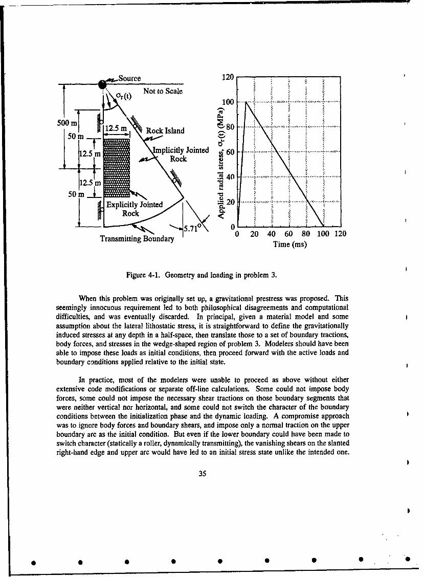
Figure 4-1. Geometry and loading in problem 3.

When this problem was originally set up, a gravitational prestress was proposed. Thisseemingly innocuous requirement led to both philosophical disagreements and computationaldifficulties, and was eventually discarded. In principal, given a material model and someassumption about the lateral lithostatic stress, it is straightforward to define the gravitationallyinduced stresses at any depth in a half-space, then translate those to a set of boundary tractions,body forces, and stresses in the wedge-shaped region of problem 3. Modelers should have beenable to impose these loads as initial conditions, then proceed forward with the active loads andboundary conditions applied relative to the initial state.

In practice, most of the modelers were unable to proceed as above without eitherextensive code modifications or separate off-line calculations. Some could not impose bodyforces, some could not impose the necessary shear tractions on those boundary segments thatwere neither vertical nor horizontal, and some could not switch the character of the boundaryconditions between the initialization phase and the dynamic loading. A compromise approachwas to ignore body forces and boundary shears, and impose only a normal traction on the upperboundary arc as the initial condition. But even if the lower boundary could have been made toswitch character (statically a roller, dynamically transmitting), the vanishing shears on the slantedright-hand edge and upper arc would have led to an initial stress state unlike the intended one.

35

) .0 0 0 0 0 0 0 0

Furthermore, even if a reasonable initial stress state could have been defined, the introduction ofa tunnel in problem 4 would have raised a whole new set of issues, differences of opinion, anddifficulties. For example, one point of contention would have been whether to impose theprestress after the tunnel is emplaced, or to computationally "excavate" the tunnel in an alreadyprestressed rock mass. In light of all the potential pitfalls, the limited insight into realcomputational differences that would have been gained compared with the effort that would havebeen required, and the small anticipated impact on the results even if the loads were imposedcorrectly, the gravitational prestress was abandoned.

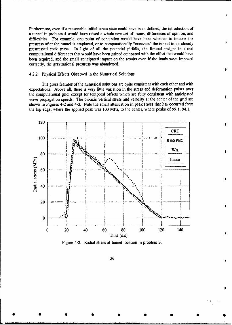
4.2.2 Physical Effects Observed in the Numerical Solutions.

The gross features of the numerical solutions are quite consistent with each other and withex"pectations. Above all, there is very little variation in the stress and deformation pulses overthe computational grid, except for temporal offsets which are fully consistent with anticipatedwave propagation speeds. The on-axis vertical stress and velocity at the center of the grid areshown in Figures 4-2 and 4-3. Note the small attenuation in peak stress that has occurred fromthe top edge, where the applied peak was 100 MPa, to the center, where peaks of 99.1, 94.1,

120 : '

"CRT10 0 .................. .. .... ...? £, ... .................... .......... ........ . ... .. .. ... ....... .. ... .... ....

4.:' RE/SPEC

80 WA

.. .. .. .

80 ....... ... ." .... ............ ..•... ....60i ...............S6 0 ............................. .... ....... -.. ......... ..................

"•40

2 -- --- --- --- ......

20

0 20 40 60 80 100 120 140Time (ms)

Figure 4-2. Radial stress at tunnel location in problem 3.

36

0 0 0 0 0 0 0 0 0

15

CRT

RE/SPEC

10 ... .... .... .... .. ..LLNL

WAS. :... .•. :; : ..............

"" Itasca•, , . °°........

...... . ...................... . ......................... ....... ..

0 d 'ri! : :: , , S I

V I,

-5 L I L j.I ... .. I . I I0 20 40 60 80 100 120 140

Time (ms)Figure 4-3. Radial velocity at tunnel location in problem 3.

94.7, and 100.8 MPa were reported by CRT, WA, Itasca, and RE/SPEC. Attenuation can betraced either to geometric divergence or material dissipation. The pure geometric divergence ofthe region over this range is slight: R -12 is only 5 percent smaller at the center than the top.Furthermore, the effective anisotropy induced by the joints might be focussing energy in thedownward direction.

Note that the LLNL approach produced a fairly accurate velocity pulse. This is probablya reflection of the fidelity of the overall uniaxial compressibility as lumped into the joints.

Another indicator of divergence is the post-peak shape of the strain path. Figure 4-4shows calculated strain paths at R=500 in, 0=2, in implicitly jointed rock. They present amacroscopic view of the deformation of a homogeneous effective medium with the properties ofintact rock and joints combined and smeared out. In this medium, as in any homogeneousmedium under rapidly rising but slowly decaying divergent dynamic loading, the strain path isalmost purely uniaxial up to the initial peak (i.e., very little hoop strain), but on unloading thehoop strain becomes increasingly negative (tensile) as outward radial displacement accumulates.

37

• • •• • •• • "

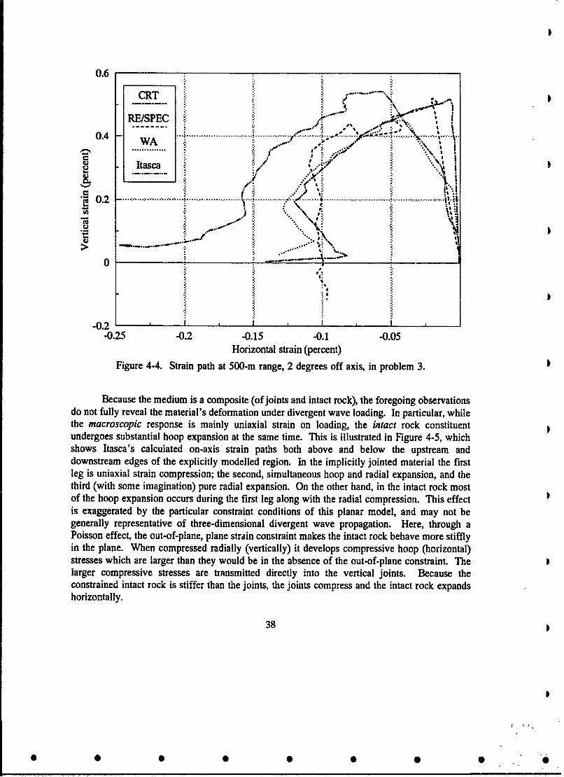
0.6

CRT .00

RE/SPEC ,

0 . . • .. . .. .-... .. ....... .. .. ...- . .. e . . .... •..., ..... , •.•..... ........... .......... ,.......-0.4

WA :, ..

,_• .............. : 00Itasca

AI

0.2 .,-' ". •, WI

0.2 . ................ ...... ..... .. .....

0 _ _ _ _ ,' . . . ,

;4

0I

-0.21 ________£________ ________ _______ _

-0.25 -0.2 -0.15 -0.1 -0.05Horizontal strain (percent)

Figure 4-4. Strain path at 500-m range, 2 degrees off axis, in problem 3.

Because the medium is a composite (of joints and intact rock), the foregoing observationsdo not fully reveal the material's deformation under divergent wave loading. In particular, whilethe macroscopic response is mainly uniaxial strain on loading, the intact rock constituentundergoes substantial hoop expansion at the same time. This is illustrated in Figure 4-5, whichshows Itasca's calculated on-axis strain paths both above and below the upstream anddownstream edges of the explicitly modelled region. In the implicitly jointed material the firstleg is uniaxial strain compression; the second, simultaneous hoop and radial expansion, and thethird (with some imagination) pure radial expansion. On the other hand, in the intact rock mostof the hoop expansion occurs during the first leg along with the radial compression. This effectis exaggerated by the particular constraint conditions of this planar model, and may not begenerally representative of three-dimensional divergent wave propagation. Here, through aPoisson effect, the out-of-plane, plane strain constraint makes the intact rock behave more stifflyin the plane. When compressed radially (vertically) it develops compressive hoop (horizontal)stresses which are larger than they would be in the absence of the out-of-plane constraint. Thelarger compressive stresses are transmitted directly into the vertical joints. Because theconstrained intact rock is stiffer than the joints, the joints compress and the intact rock expandshorizontally.

38

of te hop xpasio occrs urig te frstleg lon wih te rdia comresion Ths efec

is 0xgeae ytepriua cosritcniin 0fti 0lnrmdl an0a o be

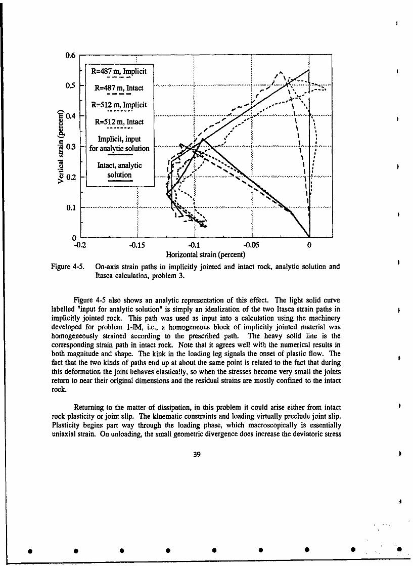
0.6

R=487 m, Implicit0.5 =487 , I tact ............ !i.... ..................... %i." ........ ..,"

0-5 R=487 m, Intact

R=512 mn, Implicit.... . .... ... ..... . .,e ...... . ... .. .-.. •.-..

C 0.4 - e % IR=512 m, Intact

C Implicit, inputS0.3 for analytic solution ............. . ......

Intact, analytic -• _ ~ ~so lution ..... •.I......................! . .....;> 0.2 ...

0.1 . ...... s..... ..... ........................... .....

0.10 - I I ... _ _ __I_ _

-0.2 -0.15 -0.1 -0.05 0Horizontal strain (percent)

Figure 4-5. On-axis strain paths in implicitly jointed and intact rock, analytic solution andItasca calculation, problem 3.

Figure 4-5 also shows an analytic representation of this effect. The light solid curvelabelled "input for analytic solution" is simply an idealization of the two Itasca strain paths inimplicitly jointed rock. This path was used as input into a calculation using the machinerydeveloped for problem 1-IM, i.e., a homogeneous block of implicitly jointed material washomogeneously strained according to the prescribed path. The heavy solid line is thecorresponding strain path in intact rock. Note that it agrees well with the numerical results inboth magnitude and shape. The kink in the loading leg signals the onset of plastic flow. Thefact that the two kinds of paths end up at about the same point is related to the fact that duringthis deformation the joint behaves elastically, so when the stresses become very small the jointsreturn to near their original dimensions and the residual strains are mostly confined to the intactrock.

Returning to the matter of dissipation, in this problem it could arise either from intactrock plasticity or joint slip. The kinematic constraints and loading virtually preclude joint slip.Plasticity begins part way through the loading phase, which macroscopically is essentiallyuniaxial strain. On unloading, the small geometric divergence does increase the deviatoric stress

39

0 • 0 • 0, 0

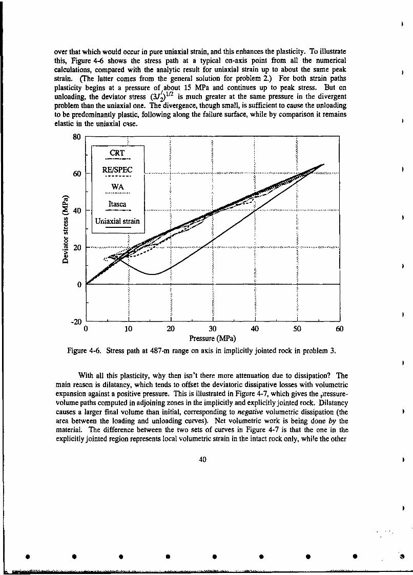
over that which would occur in pure uniaxial strain, and this enhances the plasticity. To illustratethis, Figure 4-6 shows the stress path at a typical on-axis point from all the numericalcalculations, compared with the analytic result for uniaxial strain up to about the same peakstrain. (The latter comes from the general solution for problem 2.) For both strain pathsplasticity begins at a pressure of about 15 MPa and continues up to peak stress. But onunloading, the deviator stress (3J2 is much greater at the same pressure in the divergentproblem than the uniaxial one. The divergence, though small, is sufficient to cause the unloadingto be predominantly plastic, following along the failure surface, while by comparison it remainselastic in the uniaxial case.

80

CRT

60S...............!

S~~~~Itasca • :i !

Uniaxial strain

.T 20 : ' • • .................... :L:

~0

20

-0 I0 10 20 30 40 50 60

Pressure (MPa)

Figure 4-6. Stress path at 487-m range on axis in implicitly jointed rock in problem 3.

With all this plasticity, why then isn't there more attenuation due to dissipation? Themain reason is dilatancy, which tends to offset the deviatoric dissipative losses with volumetricexpansion against a positive pressure. This is illustrated in Figure 4-7, which gives the pressure-volume paths computed in adjoining zones in the implicitly and explicitly jointed rock. Dilatancycauses a larger final volume than initial, corresponding to negative volumetric dissipation (thearea between the loading and unloading curves). Net volumetric work is being done by thematerial. The difference between the two sets of curves in Figure 4-7 is that the one in theexplicitly jointed region represents local volumetric strain in the intact rock only, while the other

40

0 0 0 0 0 0 0 • o

4 70

o RT....imp : :.-" -

40 WA-Imp *.%:/i'f :! ..".•0 .,':

S30 I WA-Exol | < ""/ --1/:;: 4"", ?• ,.•" i

' LI Itasca:m- l p / I" li .. '_.#,•." /,- . ..... ..... ........ ... .. , .,,..

20 Tac-ExpI / A5 0 R E S-C- p.' .. . " -".......... .......... .... .. .'' ...... ...... ...... ..... . . . .

4 0 ... ........... .. ...... . .i. ................ ...........! ....................IiI

Itasc-Im

r .. ........-0.2 0 0.2 0.4 0.6


Figure 4-7. Compressibility at 487-m range on axis in problem 3.

set shows overall volumetric strain including the portion due to the joints. (There is only onevalue of pressure; it is the same in intact rock as in implicitly jointed rock.) The volumetricstrain due to the joints is entirely elastic, positive, and recoverable (compressive), while tihe intactmaterial contributes a positive elastic portion and-after the onset of plasticity at about 15 MPapressure-a negative (expansive) plastic dilatant portion. Under the constraint conditions here,at low pressure the elastic volumetric strain in intact rock is about one third of the total elasticstrain. This fraction increases as the joints stiffen with pressure (in the limit of very largepressure the joints would become rigid and all the elastic strain would be in the intact rock). Thedilatancy accumulates continuously during both the post-yield portion of the loading phase andthe plastic portions of the unloading. Referring to Figure 4-7, during )oading the dilatant volumestrain is the horizontal distance between the actual curve and the extrapolation of the initial(elastic) part to higher pressures. During unloading, the additional dilatant volume strain is thehorizontal distance between the unloading and loading curves. At the same piessure, thesehorizontal distances should be the same in the implicit curve as the intact one, since there is noplasticity in the joints. Consequently, the areas representing work done by the material will bethe same regardless of which type of pressure-volume curve is used.

441

0 0

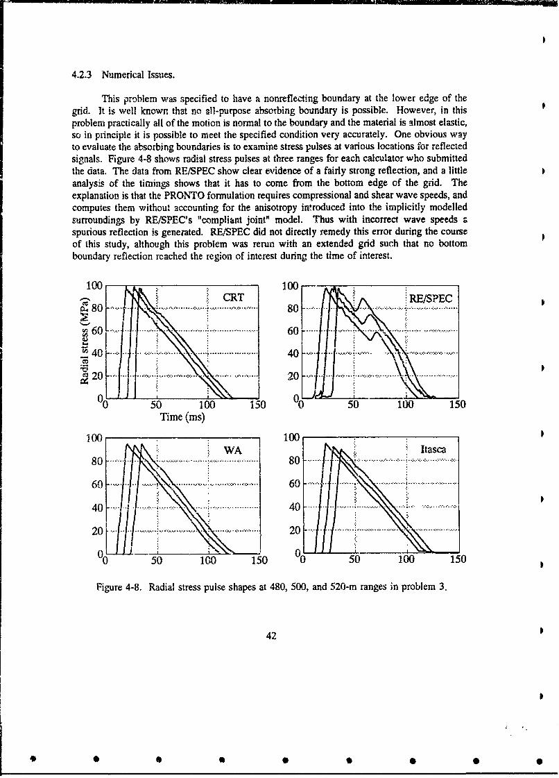
4.2.3 Numerical Issues.

This problem was specified to have a nonreflecting boundary at the lower edge of thegrid. It is well known that no all-purpose absorbing boundary is possible. However, in thisproblem practically all of the motion is normal to the boundary and the material is almost elastic,so in principle it is possible to meet the specified condition very accurately. One obvious wayto evaluate the absorbing boundaries is to examine stress pulses at various locations for reflectedsignals. Figure 4-8 shows radial stress pulses at three ranges for each calculator who submittedthe data. The data from RE/SPEC show clear evidence of a fairly strong reflection, and a littleanalysis of the timings shows that it has to come from the bottom edge of the grid. Theexplanation is that the PRONTO formulation requires compressional and shear wave speeds, andcomputes them without accounting for the anisotropy introduced into the implicitly modelledsurroundings by RE/SPEC's "compliant joint" model. Thus with incorrect wave speeds aspurious reflection is generated. RE/SPEC did not directly remedy this error during the courseof this study, although this problem was rerun with an extended grid such that no bottomboundary reflection reached the region of interest during the time of interest.

100 1001-%0 CRT :'RE/SPEC

4 5Q 10 0

820 80' ....<

J __51015(150 100 150Time (ins)

100 100WA 8..[Itasca

80 1.. .. ...... . . 80 ......

60. . . . . . .................... -- .........

400 .... 40 .....

50 100 150 50 100 1500 150

Figure 4-8. Radial stress pulse shapes at 480, 500, and 520-m ranges in problem 3.

42

• • •• • •• •

A related issue concerns the continuity between the implicitly and explicitly modelledregions. In principle the boundaries should be invisible to waves which are long compared tojoint spacing. In this problem the rise time is 10 ms and the loading wave speed is about2.5 m/ms, so the stress rise-the shortest feature of the wave-is spread out over about 25 m.Since the joints are only 1 m apart one would not expect to see much effect of theimplicit/expiicit boundary. In Figure 4-8 there is no obvious sign of reflections from theseboundaries. Another diagnostic of possible material discontinuity is the difference in computedhorizontal stres pulses on either side of the boundary; they should be equal. These traces at thedownstream, on-axis discontinuity are shown in Figure 4-9. None of the calculations gives aperfect match, but CRT and RE/SPEC are quite close, while WA and Itasca differ by 20 percentor more over most of the pulse. The discrepancy may be relatea to the fact that both WA's andItasca's implicit models are isotropic (Appendices D and E), while as noted above the overallbehavior of the jointed rock mass is orthotropic. Note, however, that by adjusting Poisson's ratioeven an isotropic material could be made to give nearly the correct coupling between horizontaland vertical stresses and strains, and therefore to provide the same horizontal stresses in theimplicitly and explicitly jointed regions when the wave traverses that boundary. Apparently WAand Itasca used some other criterion for selecting the material properties in the implicitly jointedregion. The orthotropic elastic idealization is discussed further in Section 4.3.3.

40 40::CRT : RE/SPEC

~'2 ~.: ....... 20.........

10 . ... ....I I :

10 - - .... . ....

.0 0 0 ..1 0 ...... ...

050 100 150 50 100 150

Time (ms)

40 40iasc3Implicit WA 3 Itasca

2. 7. ................. 20 .. ..-.. . .........

10 '" 10

.. :.. ... ---

-10 1001-0 50 100 150 0 5b 100 150

Figure 4-9. Hoop stress at 512-m range on axis, implicit and explicit region, problem 3.

43

• 0 0 0 0 0 0 0

4.3 PROBLEM 4: LINED TUNNEL IN A JOINTED ROCK ISLAND SUBJECTED TODIVERGENT WAVE PROPAGATION


The geometry and loading in this problem are shown in Figure 4-10. They are preciselythe same as problem 3, but now there is a lined tunnel in the center of the rock island. Theproperties of the liner have been listed in Tables 2-1 and 2-2. Calculators were asked to providemany diagnostics of tunnel and surrounding medium response, some of which will be discussedhere.

The LLNL methodology has no intrinsic mechanism for representing Poisson effects, i.e.,horizontal stresses caused by vertical strains. Therefore, in some cases, two different solutionsare presented, one with no horizontal stress, and a second with an externally imposed, constant,horizontal stress of 33 MPa. Unless otherwise noted, the LLNL results are for the nonvanishinghorizontal stress.

*,,Source 120 -* -* -. " .

'I c. (t) Not to Scaler ..100......! ~100

500 m 12.5 m R 80 .........Rock Island

Explicitly Jointd J0e . .........

Rock R70 -_..

20 4 6 .8 100.120

Transmitting Boundary Time (ms)

Figure 4-10. Geometry and loading in problem 4.

44

• • •• • •• •

0 0 00 0 00 0

4.3.2 Physical Effects Observed in the Numerical Solutions.

To begin this discussion, some general observations will be made. The incident pulse wasanalyzed in problem 3 and is shown in Figures 4-2, 4-3, and 4-8. It propagates at about2.5 m/ms with little change in shape. Thus the leading edge of the pulse arrives at the tunnellocation about 20 ms after application to the rock island boundary, and the peak, about 10 mslater.

It has been noted both in experiments and calculations that tunnel deformations aregenerally more severe under divergent wave loading than uniaxial loading to the same peakstress. Conventional wisdom holds that in divergent flow the post-peak radially outward motionscause rapid circumferential unloading, "loss of confinement," and consequent reduced strengtharound the tunnel, compared with unidirectional flow. We have already seen in problem 3 thatthe macroscopic free field strain path in this geometry does include post peak hoop expansion(Figures 4-4, 4-5), and that the stress path remains either on the failure surface on unloading ormuch closer to it than in untaxial strain (Figure 4-6). However, according to Figures 4-11 and4-12, which show histories of calculated crown/invert and springline closures, all participants

5 ..... .. CRT

RE/SPEC

4 LLNh=0

" : : ch =33 MPa

....... W A0 3 --- :"-- ".-..... :

"Itasca

..... ... ".. .

0I

0 , ... I , I , I , I , I ,

0 20 40 60 80 100 120 140 160Time (msec)

Figure 4-11. Crown-invert closure in problem 4.

45

• • •• • •• •

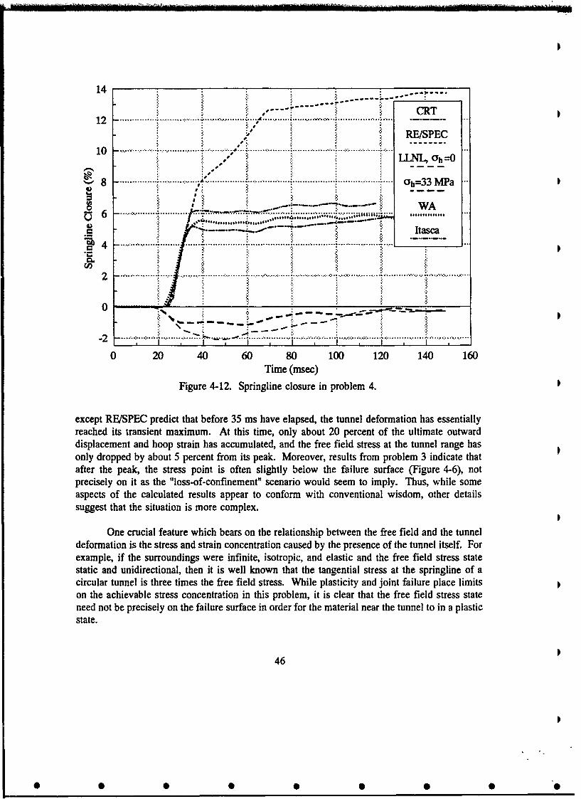
14 . . "

12,: CRT12 ............... ... ......... ' ....... .. i............... .... ............... ..... -- --

RE/SPEC10" "L' Oh=0

.......... ~....... " ............. ....... " ........... ...... ... ................ : ................. ..... ............ .. 0 h 3 ~8. ...... ch=33 MPa

4)

..... . .. ,..:,

"�" il Itasca

.--.- .. .- -. -. ,

-2 r ... -=-

0 20 40 60 80 100 120 140 160Time (msec)

Figure 4-12. Springline closure in problem 4.

except RE/SPEC predict that before 35 ms have elapsed, the tunnel deformation has essentiallyreached its transient maximum. At this time, only about 20 percent of the ultimate outwarddisplacement and hoop strain has accumulated, and the free field stress at the tunnel range hasonly dropped by about 5 percent from its peak. Moreover, results from problem 3 indicate thatafter the peak, the stress point is often slightly below the failure surface (Figure 4-6), notprecisely on it as the "loss-of-confinement" scenario would seem to imply. Thus, while someaspects of the calculated results appear to conform with conventional wisdom, other detailssuggest that the situation is more complex.

One crucial feature which bears on the relationship between the free field and the tunneldeformation is the stress and strain concentration caused by the presence of the tunnel itself. Forexample, if the surroundings were infinite, isotropic, and elastic and the free field stress statestatic and unidirectional, then it is well known that the tangential stress at the springline of acircular tunnel is three times the free field stress. While plasticity and joint failure place limitson the achievable stress concentration in this problem, it is clear that the free field stress stateneed not be precisely on the failure surface in order for the material near the tunnel to in a plasticstate.

46

0 0 0 0 S 0 0 0

Figures 4-13 to 4-16 contain a more detailed picture of the predicted stresses around thetunnel. They show the radial and tangential (with respect to the tunnel) stress distributions nearthe tunnel at two different times, free field peak stress arrival (about 30 ms) and end of positivephase (about 120 ins). Four of the calculators (CRT, RE/SPEC, and Itasca) provided results inthis form. The curves labelled "elastic" in the first two figures will be discussed later.

First consider the radial stresses (with respect to tunnel centerline) at peak stress arrival(Figure 4-13). According to the results of problem 3 the free field vertical stress at the tunnelrange is about 100 MPa and the horizontal stress about 30 MPa. At this time the free fieldstresses will decrease with either increasing or decreasing range from the source point, by about40 or 5 percent respectively over the 12.5 m (2.5 diameters) plotted. While the calculated radialstresses 12.5 in above the tunnel do exceed those an equal distance below (as expected), neitherlevel is as high as the corresponding free field value. This indicates that the relief provided bythe tunnel wall has an effect at least this far out in the vertical direction. Along a horizontalradial, however, the calculated radial stresses approach the free field horizontal stress of 30 MPamuch more quickly.

Note in Figure 4-13 that radial stresses along all radials approach about 8 MPa at thetunnel wall. This is the pressure exerted by the yielding perfectly plastic liner in the "breathing"mode.

Figure 4-14 clearly shows the concentration of tangential stress along the horizontal radial.Peak reported values range between 120 and 160 MPa, compared to the free field stress in thesame direction of about 100 MPa. However, these peaks are not as high as an isotropic elasticanalysis would predict. The reason, as noted above, is that the plasticity limits the level ofachievable stress concentration, particularly in the presence of the relief afforded by the tunnelwall.

The "sawtooth" variation of horizontal stress along the vertical radials in Figure 4-14 isdue to target point locations alternating between intact rock and joints. There is no requirementthat horizontal stresses in horizontal joints be continuous with those in adjoining intact rock. Itis comforting to note that most calculations approximately agree on the shapes and magnitudesof these curves.

Thus many features of the stress states at 30 ms can easily be explained based onintuitive, static analysis, and more will be explained later based on an orthotropic elastic analysis.In contrast, the picture at the end of the positive phase (Figures 4-15 and 4-16) is not nearly asclear. The only stresses present are either dynamic or residual, and the levels are much loweron the average. One reason for RE/SPEC's larger values compared with the others is that theyplotted results at the end of their free-field positive velocity phase, which came earlier than theothers (see Figure 4-3), while the free-field stress was still moderately compressive (seeFigure 4-2).

Figures 4-17 and 4-18 show the slip along the first four horizontal joints above the tunnelcenterline at two times, peak free-field stress arrival and end of positive phase. (All calculators

47

@ • •@ • •• •

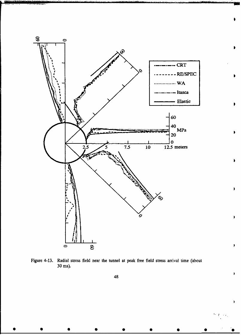
ItI

: I

: .--------. C RT

""' /--------- RE/SPEC

-d• ............. WAi•./........... Itasca

, '" Elastic

i~- 60(-4

1I

'• • •,•.• " •MPa

00

2. 5 5• • .. 7.5 10 12.5 meters

Figure 4-133. Radial stress field near the tunnel at peak free field stress arrival time (about30 ins).

48

2.5

0 0- 0- 0. 0 00,

I

------- CRT

RE/SPEC

............... W A

Itasca

Elastic

(I

-160

120

80 MPa

400

2.5 5 7.5 10 12.5 meters

Figure 4-14. Tangential stress field near the tunnel at peak free field stress arrival time (about30 ms).

49

• • •• 9 L t ) .. .. I

03

- 0 4

.10

.10

2..4. 0 25mtr

% %

Fiur 415 Rdalstes fel ea te unela te ndofth re-fel psiie hae abu

120 ms)

so

03

-i--i-F: -

.... 1

"'-'•?i " ..f,•',•CRT

---- ---- ---- ---- ---- RE/SPEC- ,,,.-

"30

2.5 5 7.5 10 12.- " e10

Figure 4-16. Tangential stress field near the tunnel at the end of the free-field positive phase

"(about 120 ins).

51

CRT

0.02 .--....

RE/SPEC

Itasca0.01 ...........

"... ".WAo ...................._..- ... "' - -

0.01.

0.00 # , /" "0.

0.02

" " ... xxPositive

0.01

0.00

0.02 1 1

S0.01 4'

0.000.0

•--

10 2 4 6 8

Distance from symmetry plane (in)0 .0 0 0 "" .... . .

Figure~t 41. Sli aln hrzntljonsatpakfe -fi oeld stres aria . . .

0.02 -- S '•''°•°" "52

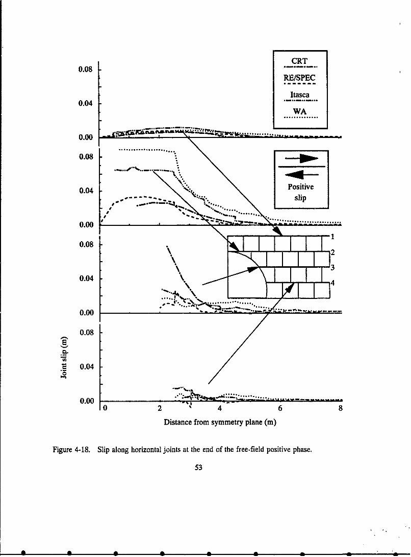
CRT0.08 ....

RE/SPEC

Itasca0.04......

WA

0.00---- -

0.08

0.04 Pstv

0.00 ~

0.08

0.04 1 1

.................................

0.00

0246 8

Distance from symmetry plane (in)

Figure 4-18. Slip along horizontal joints at the end of the free-field positive phase.

53

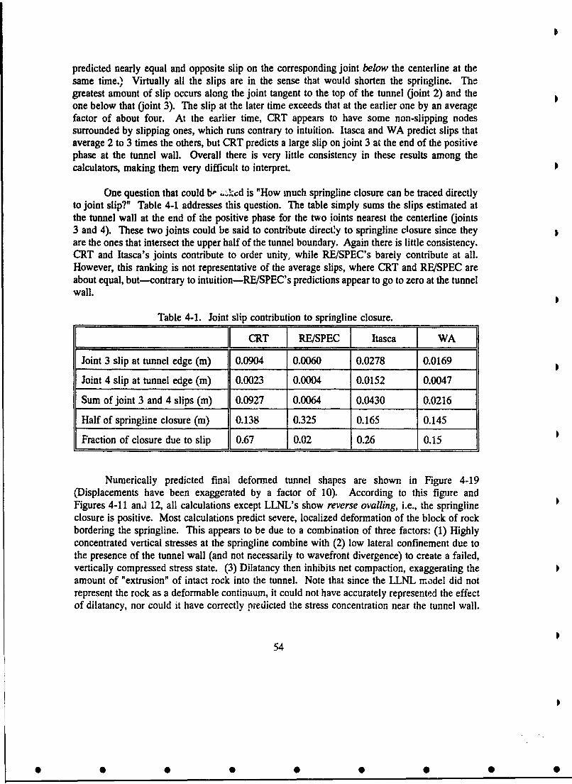
predicted nearly equal and opposite slip on the corresponding joint below the centerline at thesame time." Virtually all the slips are in the sense that would shorten the springline. Thegreatest amount of slip occurs along the joint tangent to the top of the tunnel (joint 2) and theone below that (joint 3). The slip at the later time exceeds that at the earlier one by an averagefactor of about four. At the earlier time, CRT appears to have some non-slipping nodessurrounded by slipping ones, which runs contrary to intuition. Itasca and WA predict slips thataverage 2 to 3 times the others, but CRT predicts a large slip on joint 3 at the end of the positivephase at the tunnel wall. Overall there is very little consistency in these results among thecalculators, making them very difficult to interpret.

One question that could b- -,.2!Cd is "How much springline closure can be traced directlyto joint slip?" Table 4-1 addresses this question. The table simply sums the slips estimated atthe tunnel wall at the end of the positive phase for the two joints nearest the centerline (joints3 and 4). These two joints could be said to contribute directly to springline closure since theyare the ones that intersect the upper half of the tunnel boundary. Again there is little consistency.CRT and Itasca's joints contribute to order unity, while RE/SPEC's barely contribute at all.However, this ranking is not representative of the average slips, where CRT and RE/SPEC areabout equal, but--contrary to intuition-RE/SPEC's predictions appear to go to zero at the tunnelwall.

Table 4-1. Joint slip contribution to springline closure.

I CRT RE/SPEC Itasca WA J

Joint 3 slip at tunnel edge (in) 0.0904 0.0060 0.0278 0.0169

Joint 4 slip at tunnel edge (in) 0.0023 0.0004 0.0152 0.0047

Sum of joint 3 and 4 slips (in) 0.0927 0.0064 0.0430 0.0216

Half of springline closure (in) 0.138 0.325 0.165 0.145

Fraction of closure due to slip 0.67 0.02 0.26 0.15

Numerically predicted final deformed tunnel shapes are shown in Figure 4-19(Displacements have been exaggerated by a factor of 10). According to this figure andFigures 4-11 and 12, all calculations except LLNL's show reverse ovalling, i.e., the springlineclosure is positive. Most calculations predict severe, localized deformation of the block of rockbordering the springline. This appears to be due to a combination of three factors: (1) Highlyconcentrated vertical stresses at the springline combine with (2) low lateral confinement due tothe presence of the tunnel wall (and not necessarily to wavefront divergence) to create a failed,vertically compressed stress state. (3) Dilatancy then inhibits net compaction, exaggerating theamount of "extrusion" of intact rock into the tunnel. Note that since the LLNL model did notrepresent the rock as a deformable continuum, it could not have accurately represented the effectof dilatancy, nor could it have correctly predicted the stress concentration near the tunnel wall.

54

• • •• • •• •

0 0 00 0 00 0

CRT Itasca

WA RE,/SPEC

LLNL LLNL TI_ah33 MPa ah 0

T T IC "-L '-I"T

Figure 4-19. Deformed tunnel shapes at end of positive phase (about 120 ms).Displacements are magnified by 10.

55

0 0 0 0 0 0 0 0,

4.3.3 Orthotropic Elastic Predictions of Stresses.

At a propagation speed of about 2.5 m/ms, the rising portion of the incident pulse extendsover about 25 m and the decaying portion over more than 200 in. Both of these distances arefairly large compared with the tunnel diameter of 5 m, so there is a possibility that some aspectsof the response will be quasi-static. Moreover, as noted before, the dilatancy causes the plasticresponse to be "less plastic," and in particular there is less softening on initial loading above theyield point than there would Dtherwise be. So we might expect that during initial loading, a two-dimensional, static, orthotropic, elastic solution could shed some light on the stress distributionsaround the tunnel. To this end, in this section we will construct such a solution under theloading conditions in force when the peak incident stress just reaches the tunnel center.

Tie derivation of the orthotropic elastic solution follows Lekhnitski (1966). He explainsthe general approach to two-dimensional problems using complex potentials, and provides someexamples for infinite regions with holes, but does not specifically work out the full stress fieldsfor the fundamental problem of interest here, viz., an infinite region with a hole and with uniaxialstress at infinity. So we will fill in the details needed to derive the fundamental solution, andshow how this solution can be rotated and superposed to build up one containing the effects ofvertical and horizontal free-field stress and internal pressure to represent the effect of the liner.

This first matter to be addressed is the choice of orthotropic elastic constants. In thissection only, let x, y, and z represent the horizontal, vertical, and out-of-plane directionsrespectively. The elastic relation among macroscopic normal stresses and strains in implicitlyjointed material is similar to (3-18):

EY = --vo . 1 + cry - Vz

Ee, = - vol -vcY + oz

We are interested in plane strain in the z-direction, so we set rz- 0 . The resulting expressionsfor normal strains, when compared with the standard forms

1 V2 1 12 1ex E21 7 ' Ey fl E + E2 '

56

@ @ •• @ @• @

yield

I 1 1-V2 + 12=21 v(1 +v)E 1 E 2 E wkN I-v2 + EwkN

For shear components, we write the engineering shear strain y as a sum of two parts, thefirst "-r,/G due to intact rock shearing, and the second due to joint elastic shear. For the latter,note that a square block of intact rock of any size w, bounded by joints, will suffer relativetangential displacements s/lks across each pair of parallel sides, so the corresponding shearstrain averaged over the block is 2Vx/wks . The net shear compliance is thus

1 I 2G12 G *'eS

The joint normal stiffness is the only original elastic constant that varies with stress. For thisanalysis we will hold it constant at its value when joint closure is half of joint thickness.

Next, we must solve the characteristic equation

1~ + + 2V12 1 0 1El EL G12 E)

which is a necessary condition for the general functional form of the complex potentials assumedby Lekhnitski to satisfy the equation of strain compatibility expressed in terms of stresses. Thetwo positive roots can be written

I*(I -.4E4)1/2f/2

12 " 2z

where, after using the above relations among elastic constants,

12 1 -v + 2G/wkN2 1 -v +2G/wks

The essence of Lekhnitski's procedure is that if 'I/(z),'1 2(z) are practically any complexvalued potential functions of a complex variable z, then the stress fields

57

@ • •• • •@ • "

a, - -2Re[[)14(z,) + 4 e2(z2 )]ay - 2Refe,/(Zl) + (2(Z2)]

I /

T~xy - 2hrm[,D•l(z1) + 7242(z2)1

will satisfy all the equations of two-dimensional static orthotropic elasticity provided

Zk - x +ikky , k - 1,2; i-(-I)1/2

The task now is to find potential functions for which the stresses satisfy the appropriateboundary conditions. For remote uniaxial stress 3h in the horizontal (x) direction theappropriate functions are

/ aoZ + 12 + a 2N - 1A]122 2 2-2 , k-1,22[z; + a22 Q4 Q)1(3_4 _ :k)-Akal+

where a is the radius of the opening. This completes the derivation of the fundamental solution.

The problem of interest is that of a tunnel loaded by vertical and horizontal free-fieldstresses as well as internal loads due to the liner. We will approximate the latter by a uniforminternal pressure P, . The full solution for any stress component oi can be built up bysuperposition as follows. Let 6#r, w) be the stress component at radius r from the center of thetunnel and angle co from the horizontal, corresponding to a unit remote load in the horizontaldirection. Then by linearity, the solution for horizontal free field stess 3h willbe ah 6(, o) . This corresponds exactly to the fundamental solution derived above. For theproblem of interest there are two other sources of loading, vertical free field stress oYV andinternal pressure pl. Because the implicitly jointed medium is symmetric about 450 lines, thesolution for the former is 3vf 6#, a/2 -0w). For the internal pressure we superpose three morefields: a uniform pressure p, everywhere, and the fields -pli(r,) , -pldi(rn/2 -- ) due tohorizontal and vertical free field tensions to cancel out the uniform pressure there. Thiscompletes the solution for the stresses around a statically, biaxially loaded, internally pressurizedopening in an infinite orthotropic elastic medium.

To apply this analysis to the situation at peak stress arrival time, we setov - 100 MPa, oh - 33 MPa, and Pg - 8 MPa. One final adjustment is needed: because

as already noted the free field stress varies in the vertical direction, after evaluating the stressesby superposition as described above, the result is then scaled down by an amount representingthe locally lower free field stress level. The results are plotted in Figures 4-13 and 4-14 as thecurves labelled "elastic". The agreement with numerically derived results is striking.Disagreements arise where expected, i.e., when stresses are high and plasticity comes stronglyinto play (radial stresses at --45* at intermediate radii, tangential at 0° and :900 at the tunnelwall). But the intermediate maxima in tangential stress along the AY45 radials are mimicked, and

58

• • •• • •• •

decay rates beyond the maxima in all cases are well approximated. The radial stres -s above andbelow the tunnel (Figure 4-13) closely agree with the numerical solutions. This confirms theearlier statements concerning the extent of the relief provided by the tunnel wall.

In Figure 4-14 the vertical scale for tangential stress was cut off at 160 MPa for clarity,owing to the very large stress concentrations in the elastic solution. In particular, the tangentialstress at the tunnel wall along the horizontal radial comes out at 673 MPa. This compares witha value of 259 MPa from an isotropic elastic analysis under the same loading conditions. In theorthotropic elastic solution the high stress concentration is very localized near the tunnel wall.In the first meter, the tangential stress drops to 144 MPa, i.e., by a factor of 4.7. As such, theorthotropic elastic solution would not be expected to accurately represent the stresses near thetunnel in an explicitly jointed medium, even if the blocks and joints remained elastic. However,the more severe concentration under homogeneous orthotropic conditions (compared withisotropic) suggests that the global orthotropy of the jointed medium may be leading to moresevere tunnel deformations than would arise in an isotropic medium with the same vertical andhorizontal properties.

4.3.4 Remarks on the Numerical Solutions to Problem 4.

Three of the five participants (CRT, WA, Itasca) obtained numerical solutionswhich-where comparisons were possible-agree with each other in most practical respects. Allof these solutions appear credible, based on the significant body of evidence available, i.e.,

"* Use of rational continuum models to represent the rock,

"* Use of physically based models for the joints,

"* Compatibility of results with basic understanding of wave propagation processes,

"* Absence of obvious numerical artifacts such as spurious reflections,

Comparison of stresses and strains with complete and partial analytic solutions inall the benchmark problems.

RE/SPEC's numerical solution to problem 4 differs significantly from the first three, forexample in springline closure (Figure 4-12), radial stresses above and below the tunnel at peakstress arrival (Figure 4-13), and radial and tangential stresses along the other radials at the endof the positive phase (Figures 4-15 and 4-16). In the case of the stresses at the peak stress arrivaltime, RE/SPEC's solution also differs from the orthotropic elastic solution, while the latter agreeswell with CRT and Itasca's numerical results and does so for reasons that we believe weunderstand. The large springline closure could be related to a spurious, compressive reflectionfrom the lower boundary of the computational grid. There is no obvious explanation for thesignificant residual stresses around the tunnel at the end of the positive phase (Figures 4-15 and4-1f:). There do appear to be explanations for most of the other identified shortcomings andbreakdowns in RE/SPEC's numerical solutions to the earlier problems, and with further effort the

59

@ @ @@ @ @@ •

results could probably be corrected. However, the totality of evidence developed during thisstudy suggests that this solution to problem 4 is not as accurate as the aforementioned three.

LLNL's approach omits a great deal of pertinent physics, most glaringly the behavior ofthe rock as a deformable continuum. A glance at Figure 4-19 shows convincingly that when theblocks as specified in problem 4 are permitted to deform, they will do so, and their deformationswill contribute substantially to the conventional indices of tunnel distress, viz., tunnel closure.Moreover, particularly with respect to springline closure, the coupling between vertical andhorizontal stresses and deformations plays a crucial role. There is no mechanism in the LLNLmodel for directly representing this coupling. LLNL attempted to approximate the effect byimposing a constant 33 MPa horizontal stress. The result is seen in Figure 4-12: even with theimposed horizontal stress, the springling closure is still negative (i.e., the springline elongates),in contrast with the expected result in the face of dilatant rock response. More generally, thepattern of deformations depends crucially on the distribution of stresses near the tunnel, and theLLNL approach cannot accurately estimate these stresses. It is for these reasons that theapproach seems ill-suited for the problems at hand. This is not to say that there aren't certainproblems for which it may be applicable. But to be useful it would have to be accompanied byguidelines for its applicability.

60

• • •• • •• •

• • w I

SECTION 5

CONCLUSIONS

The primary objective of the benchmark calculation study was to understand the effectof computational approach on predictions of tunnel deformations. We can only claim successin meeting that objective by adopting a rather broad view of what comprises a computationalapproach. That is, we must include more than purely numerical issues. In most cases where wehave identified problems or differences and where there is an apparent cause, that cause lies inthe way the medium was idealized. For example,

(1) The LLNL approach oversimplified the continuum physics of the rock by lumpingit in the joints, and this probably led to their substantially different results fromall the others.

(2) In some early solutions by WA the normal stiffness of the joints was based on theproperties of the intact rock and therefore unrepresentative of the specified jointstiffness. The code was modified so that a constant stiffness approximating theactual normal joint stiffness could be specified. The joints still did not have thespecified nonlinear behavior, but they did have a constant stiffness much closerto the average over the expected range of joint closures. With this modification,the reason for the stiffness deviation was understood, and was due to a consciouschoice in an area that could now be regarded as material idealization.

(3) Itasca and WA both chose to use an isotropic model for the implicitly jointedregion. A possible result of this is the discrepancy in horizontal stresses acrossthe implicit/explicit boundary noted in Figure 4-9.

There are also a few examples of issues more clearly and classically numerical in nature:

(4) The WA sliding interface model was causing a great deal of numerical chatter inproblem 2, the first one in this study where it was used. After changing certainfeatures of the model other than the stiffness (see Section E4), the problem wasresolved.

(5) RE/SPEC had a problem with the nonreflecting boundary in problem 3, andrecognized that it was caused by the wave speeds used in the boundary condition.They did not elect to remedy the problem during the course of this study. Thespurious bottom reflection probably caused higher stresses at the end of the freefield positive phase (compared with other participants), and this in turn may haveled to significantly larger spfingline closures.

It is important to recognize that there is no definitive proof of the cause-and-effectrelationships suggested above. They rely more on physical reasoning and induction than

61

• • •• • •• •

deduction. In fact, as indicated for example in the discussion on divergent flow, glib physicalarguments may either fail or reveal themselves as oversimplifications when placed under closerscrutiny.

In particular, statement (3) above, while apparently logical, could be questioned. Assuggested in Section 4.2.3, by judicious choice of material parameters, an isotropic elastic modelcould be made to give the same coupling between vertical and horizontal stresses and strains asan orthotropic one. The material parameters quoted in Appendix E for WA's implicit modelcorrespond to a smaller Poisson's ratio than for intact rock, as do the anisotropic elasticrelationships of Section 4.3.3, when used with the unstrained stiffness of the joints. But as thejoints compress and stiffen, Poisson's ratio increases. The situation is obviously more complexthan first meets the eye.

As to the overall success of the calculations themselves, the remarks in Section 4.3.4summarize the author's evaluation. But even the organizations which appeared to successfullynegotiate problem 4 did not do so without breakdowns and detours along the way. If the tunneldeformation calculations had not been preceded by a sequence of progressively more challengingproblems, the results would have been much more scattered. Often a calculator is faced with amore complex problem than any of those treated here, and fewer resources to devote to it. Someof the lessons are obvious: the calculator should take care to include all the correct physics hecan, while the customer should support as much preliminary work as possible, and barring that,maintain a healthy sense of skepticism about the outcome of any isolated, complex, numericalsimulation.

62

• • •• • •• •p

SECTION 6

REFERENCES

Allen, M.P., and Tildesley, D.J., Computer Simulations of Liquids, Clarendon Press, Oxford,1987. (UNCLASSIFIED)

Bandis, S.C., Lumsden, A.C., and Barton, N.R., "Fundamentals of Rock Joint Deformation,"Intern. J. Rock Mech. Mining Sci. & Geomech. Abstr., Vol. 20, No. 6, pp. 249-268, 1983.(UNCLASSIFIED)

Bathe, KJ. and Wilson, E.L, Iding, R.H., NONSAP: Structural Analysis Program for Static andDynamic Response of Nonlinear Systems, Report No. UC SESM 74-3, February 1974.(UNCLASSIFIED)

Bathe, K.J., and Wilson, E.L., Numerical Methods in Finite Element Analysis, Prentice-Hall,Englewood Cliffs, NJ, 1976. (UNCLASSIFIED)

Belytschko, T., "An Overview of Semidiscretization and Time Integration Procedures,"Computational Methods for Transient Analysis, Chapter 1, pp. 1-65, Elsevier Science Publishers,B.V., New York, 1983. (UNCLASSIFIED)

Callahan, G.D., and Fossum, A.F., Quality Assurance Study of the Special Purpose FiniteElement Program SPECTROM: II. Plasticity Problems, ONWI-141, prepared by RE/SPEC Inc.,Rapid City, SD, for the Office of Nuclear Waste Isolation, Battelle Memorial Institute, Columbus,OH, 1982. (UNCLASSIFIED)

Callahan, G.D., Fossum, A.F., and Svalstad, D.K., Documentaton of SPECTROM-32: A FiniteElement Thermomechanical Stress Analysis Program, DOE/CH/10378-2, prepared by RE/SPECInc., Rapid City, SD for the U.S. Department of Energy, Chicago Operations Office, 1989.(UNCLASSIFIED)

Chen, W.F. and Han, DJ., "Plasticity for Structural Engineers," Springer-Verlag, New York,1988. (UNCLASSIFIED)

Cundall, PA., Rational Design of Tunnel Supports: A Computer Model for Rock Mass BehaviorUsing Interactive Graphics for the Input and Output of Geometric Data, US Army Corps ofEngineers, Technical Report MRD-2-74, Vicksburg, MS, 1974. (UNCLASSIFIED)

Cundall, P.A., "Adaptive Density-Scaling for Time-Explicit Calculations," in Proceedings of the4th International Conference on Numerical Methods in Geomechanics, pp. 23-26, 1982.(UNCLASSIFIED)

63

• • •• • •• •

Cundall, PA., and Hart, R.D., Analysis of Block Test No. I Inelastic Rock Mass Behavior: Phase2 - A Characterization of Joint Behavior (Final Report), Itasca Consulting Group, RockwellHanford Operations, Subcontract SA-957, March 1984. (UNCLASSIFIED)

Cundall, P.A., and Lemos, J.V., "Numerical Simulation of Fault Instabilities with theContinuously-Yielding Joint Model," Rockbursts and Seismicity in Mines, A. A. Balkema,Rotterdam, pp. 147-152, 1990. (UNCLASSIFIED)

Dimagio, F.L. and Sandier, I.S., "Material Model for Granular Materials," J. of Eng. Mech. Div.,ASCE, Vol. 97, 1971. (UNCLASSIFIED)

Flanagan, D.P. and Belystchko, T., "A Uniform Strain Hexahedron and Quadrilateral withOrthogonal Hourglass Control," Intern. J. aismer. Methods in Eng., Vol. 17, pp. 679-706, 1981.(UNCLASSIFIED)

Flanagan, D.P. and Belystchko, T., "Eigenvalues and Stable Time Steps for the Uniform StrainHexahedron and Quadrilateral," J. AppL Mech., 84-APM-5. Transactions of the ASME, 1984.(UNCLASSIFIED)

Goodman, R.E., Methods of Geological Engineering in Discontinuous Rocks, West PublishingCompany, New Ycrk, 1976. (UNCLASSIFIED)

Halquist, J.0., Goudreau, G.L., Benson, D.J.,"Sliding Interfaces with Contact-impact InLarge-Scale Lagrangian Computations," Computer Methods in Appl. Mech. and Eng., Vol. 51,1985. (UNCLASSIFIED)

Heuze, F.E., Walton, O.R., Maddix, D.M., Shaffer, R.J. and Butkovich, T.R., "Analysis ofExplosions in Hard Rocks: The Power of Discrete Element Modeling," Proceedings Intern Con.Mech. Jointed and Faulted Rocks, Vienna, Austria, (A.A. Balkema, Brookfield, VT) pp. 21-28,April 18-20, 1990. Also, Lawrence Livermore National Laboratory, UCRL-JC-103498.(UNCLASSIFIED)

Ito, Y.M., England, R.H. and Nelson, R.B., "Computational Method for Soil Structure InteractionProblems," Computers and Structures, Vol. 13, No. 1-3, pp. 157-162, 1981. (UNCLASSIFIED)

Key, S.W., Beisinger, Z.E., and Krieg, R.D., HONDO I: A Finite Element Computer Programfor the Large Deformation Dynamic Response of Axisymmetric Solids, SAND78-0422, SandiaNational Laboratories, Albuquerque, NM, 1978. (UNCLASSIFIED)

Labreche, D.A., and Petney, S.V., The SPECTROM-31 Compliant Joint Model: A PreliminaryDescription and Feasibility Study, SAND85-7100, prepared by RE/SPEC Inc., Albuquerque, NM,for Sandia National Laboratories, Albuquerque, NM, 1987. (UNCLASSIFIED)

Lekhnitski, S.G., Anisotropic Plates, University Microfilms, Ann Arbor, MI, 1966.(UNCLASSIFIED)

64

0 0 • 0 0 0 0 "0

Lemos, J.V., A Distinct Element Model for Dynamic Analysis of Jointed Rock with Applicationto Dam Foundations and Fault Motion, Ph.D. Thesis, University of Minnesota, 1987.(UNCLASSIFIED)

Levine, H.S.,"A Two Surface Plastic and Microcracking Model for Plain Concrete," NonlinearNumerical Analysis of Reinforced Concrete, Winter Annual Meeting, ASME, Phoenix, AZ,November 1982. (UNCLASSIFIED)

Levine H.S., Ludwig C.J., Vaughan, D.K., isenberg, J., "Comparison of Two Different InterfaceApproaches for Modeling in Large Scale Interaction Problems", J. Appl. Mech., ASME, Vol. 94,1989. (UNCLASSIFIED)

Lysmer, J. and Kuhlemeyer, R.L, "Finite Dynamic Model for Infinite Media", J. Eng. Mech.Div., ASCE, Vol. 95, pp. 859-877, August 1969. (UNCLASSIFIED)

Muki, Y. Nelson, R.B. and Ito, Y.M., Numerical Modeling of Jointed Limestone, DNA FinalRepolt Contract DNA001-89-C- 0i05, 1992 (To be published). (UNCLASSIFIED)

Senseny, P.E., UTP Benchmark Definition, 29 March, 1991. (UNCLASSIFIED)

Simons, D.A., UTP Benchmark Problem 2-S Definition, 6 May, 1991. (UNCLASSIFIED)

Singh, B., "Continuum Characterization of Jointed Rock Mass," Int. J. Rock Mech. Mining Sci.& Geomech. Abstr., Vol. 10, 1973. (UNCLASSIFIED)

Taylor, LM., and Flanagan, D.P., PRONTO 2D: A Two-Dimensional Transient Solid DynamicsProgram, SAND86-0594, Sandia National Laboratories, Albuquerque, NM., 1987.(UNCLASSIFIED)

Vaughan, D.K. and Richardson, E., "FLEX Users Manual", Weidlinger Associates Report,Version 1-H.2, June 1991. (UNCLASSIFIED)

Walton, O.R., Particle Dynamics Modeling of Geological Materials, Lawrence LivermoreNational Laboratory Report, UCRL-52925, 1980. (UNCLASSIFIED)

Walton, O.R., "Explicit Particle Dynamics Model for Granular Materials," Numerical Methodsin Geomech., pp. 1261-1268, A.A. Balkema, Brookfield, VT, 1982. (UNCLASSIFIED)

Walton, O.R., Maddix, D.M., Butkovich, T.R., and Heuze, F.E., "Redirection of DynamicCompressive Waves in Materials With Nearly Orthogonal and Random Joint Sets," Am. Soc.Mech. Eng. AMD, v.117, pp. 65-72, ASME, New York, NY, 1991. (UNCLASSIFIED)

65/66

• • •• • •• • "

APPENDIX A

DESCRIPTION OF THE PRONTO2D COMPUTER CODE USED IN THEUNDERGROUND TECHNOLOGY PROGRAM BENCHMARK ACTIVITY

John Osnes (RE/SPEC), Ben H. Thacker (SwRI),and David S. Riha (SwRI)

Al. INTRODUCTION.

PRONTO2D is a two-dimensional transient solid dynamics code for analyzing largedeformations of highly nonlinear materials subjected to extremely high strain rates (Taylor, L. M.and Flanagan, D. P., 1987). It is the latest in a series of transient dynamics finite element codesthat has been developed at Sandia National Laboratories, beginning with HONDO (Key, S. W.,et al., 1978). As such, PRONTO2D contains a number of state-of-the-art numerical algorithms,including an adaptive timestep control algorithm, a robust hourglass control algorithm, a veryaccurate incremental rotation algorithm, and a robust surface contact algorithm. Four-noded,uniform-strain, quadrilateral elements with single-point integration are used in the finite elementformulation. Beyond its general capabilities, PRONTO2D was chosen for the benchmarkcalculations because new constitutive models are readily added and because a three-dimensionalderivative of the program is available (PRONTO3D) if needed by the UTP in the future.

The two features that make the UTP benchmark calculations relatively unique amonglarge-deformation solid dynamics problems are:

(1) A jointed rock mass subject to loading conditions that could result in large relativemotions (sliding) between adjacent rock blocks, and

(2) Loading conditions that could result in substantial tensile failure, plasticdeformation, and dilation within the rock blocks.

The joints also affect the elastic behavior of the rock mass by reducing its elastic moduli fromthe intact rock values. Further, the elastic moduli of jointed rock generally are nonlinearfunctions of the joint apertures.

The surface contact algorithm in PRONTO2D is directly applicable to modeling the slipbetween adjacent rock blocks. It is designed to simulate smooth, cohesionless surfaces with shearstrengths defined in terms of static and dynamic coefficients of friction. In the benchmarkproblems, the static coefficient of friction is the tangent of the joint friction angle. The frictioncoefficient does not decay during sliding, so the dynamic coefficient of friction is equal to thestatic coefficient.

The surface contact algorithm does not provide a means to model the elastic behavior ofthe joints. Consequently, the approach used in the benchmark problems is to superpose thenonlinear stress-displacement response of the joints and the linear stress-strain response of theintact rock. The result is a composite material whose elastic behavior is equivalent to a jointedrock mass. This approach has been developed and used successfully by other modelers

A-1

0 0 0 0 0 0 0 0 0

(Labreche, D. A. and Petney, S. V., 1987), and it is referred to as the Complaint Joint Model(CJM). Note that the elastic behavior of jointed rock masses as simulated by the CJM isinherently anisotropic because the stress-strain response normal to a joint set is substantiallydifferent from the response tangential to the joint set.

Nine constitutive models are available in PRONTO2D. They include an elastic-plasticmodel with a Mises yield criterion that is directly applicable to modeling the tunnel liner. Themodels also include an elastic-platic model with a two-invariant yield surface. However, theflow rule in that model is nonassociative and cannot be reduced to an associative form.Consequently, to perform the benchmark calculations, a new constitutive model (Drucker-Prager)was implemented in PRONTO2D for modeling the plastic deformation within the rock blocks.The new model also simulates the limited tensile strength of the intact rock. The CJM isincorporated within the model to simulate the elastic response of the intact rock, including jointsets.

In summary, the approach to modeling the jointed rock mass uses:

(1) The surface contact algorithm in PRONTO2D to explicitly model slip betweenrock blocks along joints.

(2) A new constitutive model that:

(a) Models the elastic behavior of the rock and joint sets as an equivalentcomposite material using the Compliant Joint Model to calculate thenonlinear, anisotropic stress-strain response of the rock mass.

(b) Simulates yield of the intact rock using an incremental plasticity methodwith a Drucker-Prager yield function and the associated plastic potentialfunction.

(c) Simulates tensile failure using a limited-tension algorithm to reduceprincipal stress components that exceed the tensile strength to the tensilestrength while maintaining the original principal stress directions.

A2. NUMERICAL FORMULATION.

A2.1 Explicit Time Integration.

The equations of motion are integrated using a modified central difference scheme inPRONTO2D. The velocities are integrated with a forward difference and the displacements areintegrated with a backward difference. This scheme is expressed as

A-2

• t •• • •• • "

f tEX - f INTalt ,,

tat +At ", at+ A tiut

Ut+ht t Ut+A t+At

where ftE"Y is the external nodal force, ft/W is the internal nodal force, m is the nodal pointlumped mass, and At is the time increment. This central differesafc operator is conditionallystable and the Courant stability limit is given by the highest eigenvalue wm0 x of the system(Bathe, K. I. and Wilson, E. L, 1976).

At S 2%0max

Flanagan and Belytschko (1984) provided eigenvalue estimates for the uniform strain

quadrilateral used in PRONTO2D.

Numerical damping is introduced in the solution by adding artificial viscosity. Thisprevents high velocity gradients from collapsing an element before is has a chance to respondand to quiet truncation frequency ringing. The technique used in PRONTO2D is to add viscosityto the "bulk" response. This generates a viscous pressure in terms of the volume strain rate.

A2.2 Four Node Uniform Strain Element.

PRONTO2D uses a four-noded two-dimensional uniform strain element in the finiteelement formulation. A one point integration of the element under-integrates the element butprovides a large computational advantage over a two-by-two integration rule. However, thisresults in a rank deficiency for the element that may cause spurious zero energy (hourglass)modes.

The mean stress-strain formulation for the uniform strain element considers only a fullylinear field. Any remaining nodal velocity field is the hourglass field. Possibly severeunrestricted mesh distortion can occur if these modes are excited. The method used inPRONT02D isolates the hourglass modes so they may be treated independently of the rigid bodyand uniform strain modes (Flanagan, D. P. and Belytschko, T., 1981).

A2.3 Material Behavior.

Several classical yield surfaces that are defined in terms of the first stress invariant andthe second deviatoric stress invariant have been used to model plasticity in rock. They includethe linear Mohr-Coulomb and the Drucker-Prager yield criteria. These criteria have beenreviewed by Callahan and Fossum (1982). The Drucker-Prager yield function was used formodeling the plasticity in the benchmark problems. This yield function is defined as

A-3

SIFT

0 0 • 0 0 0 0 "

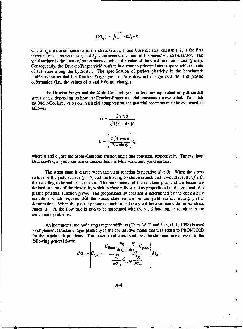
f(aij)-F, " -a11 -k

where c.ij are the components of the stress tensor, ca and k are material constants, 1 is the firstinvariant of the stress tensor, and J2 is the second invariant of the deviatoric stress tensor. Theyield surface is the locus of stress states at which !he value of the yield function is zero (" = 0).Consequently, the Drucker-Prager yield surface is a cone in principal stress space with the axisof the cone along the hydrostat. The specification of perfect plasticity in the benchmarkproblems means that the Drucker-Prager yield surface does not change as a result of plasticdeformation (i.e., the values of a and k do not change).

The Drucker-Prager and the Mohr-Coulomb yield criteria are equivalent only at certainstress states, depending on how the Drucker-Prager material constants are evaluated. To matchthe Mohr-Coulomb criterion in triaxial compression, the material constants must be evaluated asfollows:

a 2sinF 2 -sin)

k -( - sinE CO

where ý and co are the Mohr-Coulomb friction angle and cohesion, respectively. The resultantDrucker-Prager yield surface circumscribes the Mohr-Coulomb yield surface.

The stress state is elastic when the yield function is negative (f < 0). When the stressstste is on the yield surface (f = 0) and the loading condition is such that it would result in f 0,the resulting deformation is plastic. The components of the resultant plastic strain tensor aredefined in terms of the flow rule, which is classically stated as proportional to th, gradient of aplastic potential function g(oft). The proportionality constant is determined by the consistencycondition which requires that the stress state remain on the yield surface during plasticJeformation. When the plastic potential function and the yield function coincide for all stress'tates (g = .), the flow nule is said to be associated with the yield function, as required in theoenchmark problems.

An incremental method using tangent stiffness (Chen, W. F. and Han, D. J., 1988) is usedto implement Drucker-Prager plasticity in the cor ;titutive model that was added to PRONTO2Dfor the benchmark problems. The incremeqtal stress-strain relationship can be expressed in thefollowing general form: ag Of

£1jmn 00 00 Cpq tkl

.'" - rstu

Ors 0 ttlf

A-4

where doii and dek, are the components of the incremental stress and strain tensors, respectively,Cijkl are ihe components of the elastic coefficient tensor, and repeated subscripts indicatesummation. The coefficient tensor in the brackets represents the elastic-plastic tensor of tangentmoduli for an elastic-perfectly plastic material. The quantities in the brackets, including Cijkl fora nonlinear elastic material such as in the CJ'M, are evaluated at the current stress state.

For the Drucker-Prager yield surface, the partial derivatives of the yield function withrespect to the stress components are

af sij _ -abU0 Gi 2 J2

where srU are the components of the deviatoric stress tensor (sr, = or -6biI/3) and bij is theKronecker delta function. In the constitutive model added to PRONTO2D the following extendedform of the plastic potential function associated with the Drucker-Prager yield function is used:

S- F - PI -k

where

1 2sinVF3"(3 - sin V)

and V is the dilation angle. The plastic potential function results in an associated flow rule whenthe dilation angle equals the friction angle (so that B = a and g = I. The components of theflow rule (the partial derivatives of g with respect to oij) are

g . siU _ P &a Oij 2 J•

F) 2

A2.4 Limited-tension Algorithm.

A limited-tension algorithm developed by Callahan (Callahan, G. D. and Fossum, A. F.,1982) and implemented in SPECTROM-32 (Callahan, G. D., et al., 1989) is used in theconstitutive model to simulate tensile failure. In this algorithm the tensile strength at eachintegration point Tx is set initially to the intact tensile strength T.. At each integration point ateach time step, the principal stresses (a, ;. ojj - ao,,m) and their unit direction vectors( Ai, fiA1, Ail ) are calculated based on the trial stress state I at that location and time. Eachprincipal stress component that exceeds the tensile strength at tbe integration point T. is set tothe residual tensile strength T, . In addition, the tensile strength at the integration point is set toT. if Tx is exceeded. (Recall that tension is negative according to the sign convention, soexceeding Tx implies that the stress is less than -Tx and the stress is set to -Tv .) The resultantstress state is calculated by transforming the principal stress components back to the globalcoordinate system while maintaining the original principal stress directions. This transfrmationis accomplished according to the following equation:

A-5

ij -1 n1j 0y + nili niljj (lY + nJiii nJiJj all,

where n1i is the ih component L. unit direction vector Ai.

In the limited-tension algorithm, the stress state is modified in a very direct way whenthe tensile strength is exceeded. The deformation field also is affected because modifying thestress state produces an imbalance between the external forces and the internal forces (the integralof the stress divergence). In turn, this imbalance results in accelerations and ultimatelydeformation in response to the tensile failure. Changing the tensile strength to a residual valueafter tensile failure allows the formation of tension cracks to be simulated by a reduction instrength. However, this approach to simulation of tensile cracking is very crude because it doesnot account for crack orientation and the resultant anisotropy in the tensile strength. It isjustifiable wben the principal stress directions are fairly constant throughoit a simulation, so thatthe tensile direction and the resultant orientation of tension cracks are fairly constant. In general,this condition could not be ensured in the benchmark calculations. Consequently, the tensilestrength is maintained at the intact value even after tensile failure (i.e., Tr = TO).

A2.5 Implicit Rock Joint Modeling.

The compliant joint model (CJM) is a three-dimensional elastic model used to representthe mechanical response of a rock matrix with joints (Labreche, D. A. and Petney, S. V., 1997).The model implemented in PRONTO2D is a two-dimensional version of the CJM. The CJMassumes that the deformation of a jointed rock mass is caused by the combination of the elasticresponse of the rock matrix and the elastic response of the joints. The unfractured rock matrixis modeled as an isotropic linear elastic solid and the Joints as a nonlinear elastic layer. Themodel consists of up to four joint sets with various spacing and orientation. The response of theCJM is effectively anisotropic due to the presence of the joint sets.

The displacement behavior normal to the joint plane varies nonlinearly with stress and theresponse is governed by the physical characteristics such as joint aperture, roughness and contactbetween joint surfaces, strength of the wall rock, and presence or absence of filhing. Theresponse is also governed by the recent movement history of the rock joint. The aperture changeof a well-mated joint without filling can be represented by a hyperbolic relationship between thestress normal to joint plane and the joint closure (Bandis, S. C., et al., 1983 and Goodman, R. E.,1976). The form used in the CJM is given by the equation

MIOn n a"where,

an - normal stress acting on the joint (compression positive)

a - half-closure stress (stress to reduce the aperture to 6/2

v - joint normal displacement (closure positive, zero when On = 0)

8 - maximum joint closure

m - exponent

A-6

The stiffness normal to the joint, kn, is defined by

k,, n - IC m vnM - 1k - ai

O vn (8 - Vn )m

which is the slope of the nonlinear joint closure. For the Benchmark problems, a = 125 MPa andm = 1. This hyperbolic function is used in the numerical formulation for the normalstress-displacement response when the normal stress is compressive. A constant value of 10 -4times the dilatational modulus, ), + 2t, of the matrix is used for joint normal stiffness when thenormal stress is tensile. This stiffness defines a linear, normal stress-normal displacementrelationship for tsie joint in tensior. This small but nonzero stiffness avoids numericalsingularities in the computations. The transmission of small tensile stresses by elements havingmoduli four orders of magnitude lower than the matrix are accepted as insignificant relative totypical compressive stresses.

The compressive normal stress-displacement relation is nonlinear and elastic. Thus, thereis no path dependence and all joint closure is fully recoverable in this model.

The shear response of joints generally consists of a nearly linear rise to peak shearstrength, followed by softening behavior with continuing shear. However, it is acknowledged thatjoint size dependence may alter this. The peak shear strength response of joints is supported bystudies such as Goodman (1976) and Bandis (Bandis, S. C., et al., 1983). The shear stress ofjoints is known to be inelastic when the stress state approaches the peak shear strength. T'heCJM only models the elastic joint shear response. The shear stiffness, which is independent ofthe normal stiffness across the joint, relates the shear displacement to shear stress.

"c - ks vt

where,T - shear strength

k, -joint shear stiffness

v - joint displacement tangent to plane of joint

The shear stiffness is defined by

aVt

The CJM introduces anisotropy by reducing the composite modulus of the modeled rockmass in the direction normal to the joint in an otherwise linear elastic material. Computation ofeffective moduli is used to implement the softening effects of the joints. Stress equilibrium isthe underlying assumption in the combined response of the rock matrix and the joint sets. Thenormal stress across the joint is equal to the stress in the rock matrix normal to the joint plane.The shear stress on the joint is equal to the shear stress in the rock matrix parallel to the jointplane.

A-7

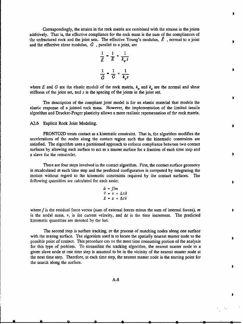
Correspondingly, the strains in the rock matrix are combined with the strains in the jointsadditively. That is, the effective compliance for the rock mass is the sum of the compliances ofthe unfractured rock and the joint sets. The effective Young's modulus, E , normal to a jointand the effective shear modulus, 6 , parallel to a joint, are

1 1 1

SE k s

1 1 1

U G ksS

where E and G are the elastic moduli of the rock matrix, kn and k. are the normal and shearstiffness of the joint set, and s is the spacing of the joints in the joint set.

The description of the compliant joint model is for an elastic material that models theelastic response of a jointed rock mass. However, the implementation of the limited tensilealgorithm and Drucker-Prager plasticity allows a more realistic representation of the rock matrix.

A2.6 Explicit Rock Joint Modeling.

PRONTO2D treats contact as a kinematic constraint. That is, the algorithm modifies theaccelerations of the nodes along the contact region such that the kinematic constraints aresatisfied. The algorithm uses a partitioned approach to enforce compliance between two contactsurfaces by allowing each surface to act as a master surface for a fraction of each time step anda slave for the remainder.

There are four steps involved in the contact algorithm. First, the contact surface geometryis recalculated at each time step and the predicted configuration is computed by integrating themotion without regard to the kinematic constraints required by the contact surfaces. Thefollowing quantities are calculated for each node:

Sv + Ata

S- x + ANO

where f is the residual force vector (sum of external forces minus the sum of internal forces), mis the nodal mass, v, is the current velocity, and At is the time increment. The predictedkinematic quantities are denoted by the hat.

The second step is surface tracking, or the process of matching nodes along one surfacewith the mating surface. The algorithm used is to locate the spatially nearest master node to thepossible point of contact. This procedure can be the most time consuming portion of the analysisfor this type of problem. To streamline the tracking algorithm, the nearest master node to agiven slave node at one time step is assumed to be in the vicinity of the nearest master node atthe next time step. Therefore, at each time step, the nearest master node is the starting point forthe search along the surface.

A-8

The next step is to determine contact or penetration. The slave node is oriented withrespect to the master segments connected to the tracked master node. The depth and positioncoordinates are calculated for both master segments connected to the nearest master node. Fromthese quantities, if the depth is positive, the slave node is penetrating the segment and if theposition is positive then the slave node is along the segment. When the master surface forms anoutside comer, there may be penetration of both segments. In this case, the algorithm determineswith which master segment the slave surface is more strongly in contact. One limitation of thealgorithm is that it can not detect a contact surface contacting itself.

The final step in the contact algorithm is to calculate the penetration forces imposed onthe master surface by the slave surface to restore kinematic compliance. These forces arecalculated as a fraction of the forces that would be imposed by the slave nodes if the mastersurface was rigid. This fraction is based on the fraction of each time step for which the surfacesact as master Wnd slave. The roles are reversed for the remaining fraction of the time step. Theaccelerations are calculated to predict the response of the master surface to these penetrationforces such that the response of each contacting slave node is constrained by its master nodes.The principle of virtual work is employed to define the accelerations of the master nodes inresponse to the penetration forces. When friction is present, the relative tangential motion of thecontacting slave nodes is resisted. The magnitude of the tangential force exerted on the mastersurface on a slave node cannot exceed the friction force. Thus friction adds a tangentialacceleration to the nodes in contact

A2.7 Transmitting Boundary Conditions.

A transmitting boundary is used to simulate a semi-infinite domain outside the boundary,where the wave speeds of the material on both sides of the boundary are the same. The regionexterior to the boundary is replaced with an energy-absorbing boundary condition that behavesas if the energy is transmitted across the boundary. Thus, no energy is reflected back into theinterior region.

The nonreflecting boundary is implemented in PRONTO2D according to a techniqueproposed by Lysmer (Lysmer, J. and Kuhlemeyer, R. L., 1969). The basic idea is to applytractions at the boundary that will exactly cancel the stresses that would be reflected from a freesurface. Hence, the numerical technique involves calculating and applying the following tractionsto the surface of the nonreflecting boundary

oF - -P V a

where on and Ts are 'the normal and shear tractions; p, V , and Vs are the current density,compressional wave speed, and shear wave speed of tle material along the boundary;and tin and a, are the normal and tangential components of the current velocity at theboundary. At each time step, PRONTO2D updates the tractions at the boundary using the currentdensity and effective dilatational and shear moduli in each element along the boundary.

In calculating the current wave speeds, PRONTO2D assumes that the wave speeds areisotropic and independent of the orientation of the boundary. Obviously, the joint sets in a rock

A-"

4 mass yield an anisotropic medium in which the wave speeds depend on the incident direction.However, the anisotropy inherent in the CJM is not accounted for in the wave speed calculationin PRONTO2D. Consequently, the wave speeds used to calculate the tractions along thenonreflecting boundary are somewhat in error, the magnitude of which depends on the orientationof the boundary with respect to the principal directions of the anisotropy. This error results ina partial reflection of the incident stress.

A-10

APPENDIX B

THEORETICAL ASPECTS OF THE LLNL DIBSDISCRETE ELEMENT CODE USED IN THE DNA/UTP

BENCHMARK EXERCISE

Francois Heuze

B1. INTRODUCTION.

Calculations for this study were performed with the LLNL Discrete Interacting BlockSystem (DIBS) numerical model (Walton, 0. R., 1982 and Walton, 0. R., 1980) using a r-w"rounded comer" version of that model. DIBS was started from the algorithms of earlier"Uistiact-riement" models (Cundall, P. A., 1974), and evolved at LLNL. It calculates the motionof each discrete polygonal block as it responds to contact forces, boundary and applied loads, andgravity. Arbitrary (convex) polygonal shapes are allowed for each particle or block. Severalsimplifying assumptions make the calculations tractable. All deformations take place at thecontacts, which include the compliance of the rock blocks as well as that of the rock joints;meanwbile the blocks are kept rigid during the calculations. Note that all rock joints in DIBSare explicit; there is no implicit jointing. All starting contacts between polygons are assumed tobe corner-on-side (i.e., temporary, sliding joint-elements or contacts are set-up at polygonalvertices, as needed). Small but finite "overlaps" occur as normal forces are developed. Similarlya finite, partially recoverable shear-strain develops in the contact before frictional sliding isinitiated. In the rounded-corner version of the model, corner-comer contacts are also allowed,and they serve to allow a smooth transition in the direction of the contact normal, as a contactmoves from one side onto the next.

DIBS has been applied to several analyses of the effects of nuclear and chemicalexplosions in jointed rocks (Heuze, F. E., et al., 1990).

B2. CONTACTS.

Information on contact detection and on corner-side contacts is available in (Walton,0. R., et al., 1991). The rounded-comer contact capability was developed for this study.

, ,- rounded-corner version builds on the DIBS construct. From a user's point of viewthe model functions almost the same as the sharp-comer version. Internally, however, there aresome significant differences. Input geometric data for each block contain the coordinates of an"outer" polygon with sham comers; this is just the polygon the original DIBS model would use.When the problem is initialized (i.e., as geometric data are stored) a circle of fixed radius, re,,is placed inside each vertex, tangent to the two adjacent sides. A new "inner' polygon isconstructed connecting the centers of each of the comer circles. The side lengths of the innerpolygon are exactly the same as the lengths of the Erne segments between tangent points on theouter polygon (Fig. B-i). The coordinates of the vertices of the inner polygon replace theoriginal outer polygon coordinates in the computer storage arrays, and this inner polygon is usedon all contact searching algorithms. Such a construct facilitates the use of most of the samesearching algorithms for contact detection as were used in the original sharp-comer version of

B-1

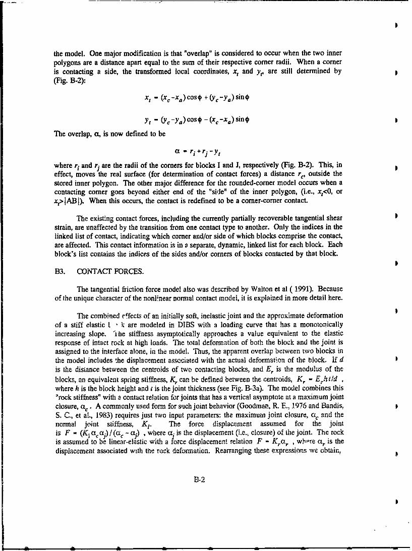
the model. One major modification is that "overlap" is considered to occur when the two innerpolygons are a distance apart equal to the sum of their respective corner radii. When a comeris contacting a side, the transformed local coordinates, x, and y,, are still determined by(Fig. B-2):

Xt - (XX -xa) Cos + (Yc-ya) sin

Yt - (Yc -Ya) Cos 0 - (xc-xa) sin 0

The overlap, a, is now defined to be

a - r+rj-y,

where r. and r- are the radii of the comers for blocks I and J, respectively (Fig. B-2). This, ineffect, moves the real surface (for determination of contact forces) a distance rc, outside thestored inner polygon. The other major difference for the rounded-corner model occurs when acontacting comer goes beyond either end of the "sidee" of the inner polygon, (i.e., x,<O, orx,> lAB I). When this occurs, the contact is redefined to be a comer-corner contact.

The existing contact forces, including the currently partially recoverable tangential shearstrain, are unaffected by the transition from one contact type to another. Only the indices in thelinked list of contact, indicating which comer and/or side of which blocks comprise the contact,are affected. This contact information is in a separate, dynamic, linked list for each block. Eachblock's list contains the indices of the sides and/or corners of blocks contacted by that block.

B3. CONTACT FORCES.

The tangential friction force model also was described by Walton et al (1991). Becauseof the unique character of the nonlinear normal contact model, it is explained in more detail here.

The combined effects of an initially soft, inelastic joint and the approximate deformationof a stiff elastic L , k- are modeled in DIBS with a loading curve that has a monotonicallyincreasing slope. "I he stiffness• asymptotically approaches a value equivalent to the elasticresponse of intact rock at high loads. The total deformation of both the block and the joint isassigned to the interface alone, in the model. Thus, the apparent overlap between two blocks inthe model includes the displacement associated with the actual deformat-on of the block. If dis the distance between the centroids of two contacting blocks, and Er is the modulus of theblocks, an equivalent spring stiffness, Kr can be defined between the centroids, K, - Eirt/diwhere h is the block height and i is the joint thickness (see Fig. B-3a). The model combines this"M rock stiffness" with a contact relation for joints that has a vertical asymptote at a maximum jointclosure, (x" A commonly used form for such joint behavior (Goodman, R. E., 1976 and Bandis,S. C., et a!., 1983) requires just two input parameters: the maximum joint closure, cr, and thenormal joint stiffness, K,. The force displacement assumed for the jointis F - (K aa.) / (ac - a.) , where a; is the displacement (i.e. closure) of the joint. The rockI C J C "

is assumed to be linear-elastic with a force displacement relation F - Krctr , wbhre c•r is thedisplacement associated with me rock deformation. Rearranging these expressions we obtair,

I~o

ri

OuterPolygon >_Verx

Figure B-1. Rounded-Comer Polygons.

i(xitYj) B (xb yb)+)

A(XaD~~a f (xv y,)

Figure B-2. Schematic of Comer-on-Side Contact in DIBS.

B-3

Fac a F

C F+Klac r Kr

for the displacements of the joint and rock, respectively. The total displacement, , is simplythe sum of these two terms,

Fac Fa m aj + ar +Klac (B-i

Equation (B-1) may be solved for F in terms of a,

F - l[aKr,-a(K +r)] + K f... +K{[(lK +K)a-aK] 2 +4KKra

The slope of this force displacement curve, dF/da , approaches Kr as a approaches infinity,

2dF Kr aKr2 - ac Kr (Kr-rK)da 2 2[a2K2 E2aacKr(K,_K1)+(Kr+K)2 a2 ]

Figure B-3a is a schematic representation of the rock-joint model and Fig. B-3b showsthe qualitative behavior of the component and combined force-displacement curves. Variousassumptions are possible for unloading and reloading with this nonlinear rock-joint model: (a)the unload and reload slopes are equal to Kr., (b) the unload and reload slopes are equal to thetangent of the loading curve at the point of initial unloading, and (c) unload and reload slopesare set to a fixed (input) multiplier of the tangent slope at initial unloading. The selection of theunloading model determines the degree of energy loss during collisions.

B4. OTHER THEORETICAL ASPECTS.

B4.1 Viscous Damping Algorithm.

Without any viscous damping, the hysteretic contact model produced some numericalnoise in wave propagation calculations. After tests of various damping options, we adoptedlinear, velocity-proportional damping, the effect of which was shown to be amplitudeindependent.

F - Ka-DV

The damping coefficient D is a user input, and it is suggested to be approximately two to fivepercent of critical damping

D - .04(KM) (B-2)

where K is the spring stiffness between blocks and M, the average block mass. Figure B-4a isa plot of position versus velocity showing the numerical noise the code was generating when asquare pulse was applied to the end of a one-dimensional chain of blocks, without any damping.

B-4

J , • . .. ... L

tI

Fd

Block Modulus E,

a) Schematic of Rock and Joint Model

Joint 1Rock RockI I MassF F F

+ KI + =Kr

II

IE j rIX

b) Force-Displacement Model for Normal Contact

Figure B-3.

B-5

1@ o... _0.-•a. ,,.10

4 4

2 2

4 ,4

4 4

-12 .121 ' ' ' ' 'Peeks" !ufte

a) No viscosity; numerical noise b) Viscosity; no numerical noise

Figure B-4.

10 10

* 6

'44

8404 4+40 - - 10 -

-12 .+ ' ' -1 2 I I I I I !

a) No infinite boundary; b) Infinite boundary;

wave reflection no wave reflection

Figure B-5.

B-6

In contrast, Figure B-4b is an illustration of the same plot as in Figure B-4a, but with the

addition of the small amount of viscous damping indicated in Equation (B-2).

B4.2 Infinite/non-reflecting Boundaries.

To absorb the wave with no reflected pulse, we added linear damping on the boundary;the dashpot coefficient used was one quarter of critical damping, as determined empirically

F-.5(KM) V (B-3)

where K is the spring stiffness and M is the block mass for blocks next to the boundary. Notethat the functional form of Equation (B-3) is equivalent to the pC damping used traditionally ininfinite boundaries for finite element grids (Lysmer, J. and Kuhlemeyer, R. L., 1969). Figure B-5a is a plot of the wave reflected from the rigid left boundary of a one-dimensional chain ofblocks, when the calculation of Figure B-4b is continued without the silent boundary capability.In contrast, Figure B-5b is the same plot but with the addition of the silent boundary capability,and it shows essentially no wave reflection. The wave absorption has proven to be very efficientin two dimensions, as well.

B4.3 Other Features.

Numerous other features were put in DIBS in the past years. They are fully explainedelsewhere (Heuze, F. E., et al., 1990), and are summarized as:

"* A new method for speeding up gravity settling. A factor of 8 in speed wasobtained by using a kinetic energy zeroing algorithm.

"* A boundary transformation algorithm to go from the gravity settling mode to theinfinite boundary mode.

"* A new contact search algorithm which eliminates spurious high forces where newcontacts are discovered.

"* A time-history capability and restart capability.

"* A variety of mesh generating algorithms, including a Voronoi polygon generator.

B5. TIME INTEGRATION.

At each explicit time step of the calculation, a loop through all contacts is perfurmedonce, accumulating the total force and moment on each particle for that configuration. Then, theequations-of-motion are integrated one time step and the time advanced. Each coordinate of eachparticle's position (i.e., x y, and 0) is integrated in time using a second order accurate schemevalid with non-uniform time steps. For example, the x-coordinate of the centroid of a particleat time step n +1 is determined explicitly from the positions at steps n and n-1 and thex-direction force at the nth time step, F , by the expression

B-7

.(It+ Xn - xAt' +n-1.+ I(At'At+At' 2)Xn...+O(At 3)n 1At) At) I

where At' is the time interval from n to nr+1, At is the time interval from n -1 to n,and fX - Fn/m where m is the mass of the block. If the time step is uniform (i.e., At' - At) ,and there are no velocity dependent forces, this expression reduces to the familiar, time centered,third order accurate Verlet scheme commonly used in molecular dynamics calculations (Allen,M. P. and Tildesley, D. J., 1987). Similar expressions are used for the y- and 0-coordinateintegrations, based on the total y-direction force and the total moment acting on each block.

Because this is an explicit integration scheme, the time step must be kept below a stabilitylimit determined by the stiffest spring and/or the smallest mass in the system. For accuracy, thetime step must usually be kept significantly smaller than the stability limit. Empirical tests ofaccuracy have determined that on the order of 50 or 100 time steps per physical oscillation cycleare needed for the numerically integrated results to compare favorably with analytic solutions forsimple multi-block systems (i.e., ±-1%).

B-8

APPENDIX C

DESCRIPTION OF FINITE ELEMENT METHOD USEDIN UTP BENCHMARK ACTIVITY

BY CALIFORNIA RESEARCH AND TECHNOLOGY

Yoshio Muki, Y. Marvin Ito

C1. INTRODUCTION.

Finite element methods which incorporate an interface logic are capable of simulating thebehavior of jointed rock masses subjected to quasi-static or dynamic loading environments. AtCalifornia Research and Technology Division (CRT) of The Titan Corporation, analyses ofjointed rock mass problems for the LTP Benchmark Activity were performed usingEXCALIBUR. Originally developed from NONSAP (Bathe, K. J., et al., 1974), a Lagrangianfinite element program for the solution of static and dynamic structural and continuum problemswith both geometric and material nonlinearity capabilities, EXCALIBUR has undergone extensivedevelopment and validation over the course of many DNA sponsored programs.

The EXCALIBUR code uses an explicit (central-difference) time integration schemewhich allows efficient solution of ground shock problems where there are large responsegradients in both time and space. An advantage of the explicit algorithm is the ability toincorporate complex constitutive models which represent detailed inelastic behavior of geologicmaterials. The code also has a variety of special features to enhance numerical solutionefficiency, including element underintegration, and controls on the levels of physical modelscarried by various parts of the finite element grid.

C2. REPRESENTATION OF JOINTED ROCK MASS.

For analyzing tunnel response in jointed rock masses, EXCALIBUR treats large-scalematerial discontinuities with gap formation and frictional contact using an interface element. Arecent enhancement incorporates substructuring at the element level allowing the code to capturemicromechanical effects including anisotropy in the far-field jointed system without increasingthe global system of equations. These methods of modeling jointed rock masses are used in theUTP benchmark calculations. The first approach, termed discrete joint modeling, will bedescribed next, followed by a description of the second approach termed composite jointed rockmodeling.

C2.1 Discrete Joint Modeling.

In the discrete joint modeling approach, both the rock mass and the rock joint arerepresented by ordinary finite elements, typically four-node quadrilaterals. The mechanicalbehavior of the rock joints is modeled using a modified version of the CRT Interface ElementfIto, Y. M., et al., 1981). The interface element was developed to treat the mechanicalinteractions of dissimilar or disconnected bodies. The element typically carries a high aspectratio with a prescribed stiffness in the direction normal to the joint face.

C-1

As specified for the Benchmark Activity, the normal stiffness of the rock joint isprescribed to increase with closure. The element has a constant elastic shear stiffness, with shearbearing capacity along the joint face following a non-dilatant Coulomb-type friction rule(dependent on the normal stress). The element can be prescribed to have no stiffness in tension.This combination of features allows the element to model interface stick, slip and separation.

The constitutive relation governing the interface element is a 2-by-2 matrix, i.e.,

{AOn}-cc1 C12] y I

where 'T and y are shear stress and strain and o, and are normal stress and strain. Underconditions where the interface is closed and no slip is occurring, the incremental constitutiverelation is

[AT ~ ;. { AA"Eyf}

where G'and E' are the tangent stiffnesses. While under conditions where slip is occurring, therelation is

{ A T 0 -Ži .E' A T T" +IIAO,4 0 T I ]{A} ;n0 E

where -r. is the cohesion and Ii is the coefficient of friction. And of course, during separation(En < 0), the stiffness is the zero.

In this method, the thickness, location (hence spacing), and orientation of the rock jointare discretely represented in the numerical model. This is an important feature of modelingjointed rock fields near buried structures where the nominal structural dimensions are of the sameorder as the nominal joint spacing. Thus, a small time step is usually required, not only to retainnumerical stability, but to accurately track the nonlinear behavior of the joint system near thetunnel.

C2.2 Composite Jointed Rock ElemenL

In order to effectively analyze jointed rock mass in the far-field, a composite joint/rockmass element has been developed (Muki, Y., et al., 1992). The composite jointed rock elementis a mathematical representation of the mechanical behavior of a rock mass with a regulardistribution of joints. The element is intended to capture the mechanical behavior of acharacteristic sample of insitu material comprising a rock mass interspersed with joint zones.Each component within the composite joint element is treated as a substructure with a full and

C-2

0 0 0 0

separate constitutive relationship. The interaction of the joint zones and rock mass is based onstress equilibrium and strain compatibility within the element.

The composite jointed rock element assumes a geometric orientation and distributionbetween intact rock and joint materials, with the intact material taking up most of the regionoccupied by the element. For the sake of this discussion, the orientation of the distribution ofjoints is taken to be horizontal and vertical, although this restriction can easily be changed toaccount for more arbitrary jointed rock mass configurations. The joint zone represents the effectsof all joints with similar orientation in the sample. The key parameter is the relative thicknessof (distributed) joint material as compared to intact rock. Since there are two types of joints,horizontal and vertical, two characteristic ratios of intact rock thickness to joint material thicknessmust be defined: the ratio of the width W of the intact material to the width w of the verticaljoint material is a - W/w >> 1, and the ratio of the height H of the intact material to the heighth of the horizontal joint is defined as P - H/h>>1.

The superscripts used in the development are as follows:

[ refers to intact rock material quantities,

[]V refers to vertical joint material quantities,

[]h refers to horizontal joint material quantities.

Also, the symbols AFc refer to correction strain and Ao' refer to out-of-balance stress.Unsi'perscripted quantities refer to overall element (external) quantities which define thecomposite representation of the response of the various components of the jointed rock mass.These composite values are used during the time integration. Finally, with the exception of out-of-balance stress terms, which are carried forward from the previous time step, all quantities arequoted at the current time step.

The following mathematical developnment assumes plane strain behavior, with x denotingthe horizontal direction and y the vertical direction. Overall composite strain increments arerepresented by AE, {AJ} - {Asx AEy AyI} and are uniform over the entire element.Correction strain increments are represented by AEc, {fAc} - {ASc A c Ayc}. The correctionstrains represent perturbations about the overall composite strains andJaffect each componentdifferently. These correction strain increments are used to adjust the increments in the strainsof both the intact rock and the vertical and horizontal joints to attain internal stress equilibrium.Note that the internal strain correction increments do not affect the motions at the four cornernodes. Together, seven strain increment modes (four internal and three external) along with thetwo material distribution parameters, a and [, fully describe the incremental strain state of eachof the components.

C-3

The governing equations for compatibility of strain increments are

Ac'x -Ac -Ac"-

AyI - Ay-1" A C-1 t"a

A E, - Ac1, -TA (C-1)

Ay' - Ay- 1 Ay' - -1 Ay4ha

for intact rock,

Acv - AE +A~c

AeV - lAE AC, C2

Ay1 - Ay+•Ay- - _Ay .hT

for vertical joint material, and

h1 CAF e -Ax -a A /x

A oh _ Aoh- ,, (C-3)

Ayhh - Ay - AY + Aycha

for horizontal joint material.

Assuming that changes in stresses produced from the strain changes in the previous timestep are not in equilibrium, an inherited out-of-balance in stress increments Ac' must be carriedforward and included in the calculation for stress equilibrium at time t. [For example,

I - I 1 I

Then, for stress equilibrium, the following equations must hold

, e +,,-cv +AdAe Ah IAo

4y 4 y (C4)Atv + A •- A-1 I

From the constitutive relationship for intact rock we have

Ax C 11 Ax + 12 A-y

A I - C I AcI + C1I A I (C-5)Gy 11 Ey 12 Fx

AT I C3 Ay'

C-4

where the stiffness coefficients d are assumed-isotropic and related to bulk modulus K1 and shearmodulus GI by the usual relations

I 141

C 12 -K +G3

I

Similar relations hold for the vertical joint material (superscript v) and for the horizoatal jointmaterial (superscript h).

Combining Equations (C-1) through (C-5) gives a set of equations relating intact rock,vertical joint and horizontal joint strain increments to nominal external and internal strainincrements, a:d corrections in the stress increments of the form:

[C] {As~}J - [D] {AEJ} -- {fLe} ((C-6)

where

..v1 11 1 1(_C20

1 1 h h + 1 C1 0 0(C - (• 1) C

0 0 -3 3+ -8c 31 3 -( c31 -I

a

I v

0 h I h11 12-C12 "1. ll 0

o 0

C;3 - 33

o C CAI-C 3 h IC33 -3333

C-5

0 0 0 •_

EC Ah Ex 0XJAE') AJy xAE A ~(` AoaAy CV Ae As Y ; AT'~

When the composite element is used in conjunction with nonlinear materials, apredictor/corrector method ito, Y. M., et al., 1981) is used to maintain solution accuracy andefficiency. Briefly, the incremental stiffness relationship in Equation (C-6) is based on secantmoduli which are calculated at the end of each time step for use in the equilibrium equation inthe following time step. If the type of loading changes (e.g., plastic loading/unloading jointseparation closure, a set of revised secant moduli can be calculated for each of the componentsundergoing the nominal external strain increment. Note that the secant moduli are for anassumed strain increment and may not be the same as for the strain increments obtained aftersolving Equation (C-6). This difference will lead to out-of-balance stress I Aoe, which isadded in the following time step.

Given the material moduli, overall strain increments and out-of-balance, Equation (C-6)can be solved for the internal strain incremenets. For elastic conditions, Equation (C-6) isdecoupled into two 2-by-2 systems of equations which are easily solved for { A FC }. Insertionof { A ,C} into the strain compatibility relationships (Equation2 C-3, C-2, C-3) yields thepredicted equilibrium strains for each component of the element. Stresses and other statevariables are then updated by exercising the appropriate material model for each of thecomponents in the new strain state. By using the pred;ctoricnnector method, the rumber of calls

to the material mczel subroutines can be minimized.

Finally, it is also po:,sible and often desirable to use the initial elastic moduli for each ofthe materials in the internal equilibrium equatioais for all time, even though larger approximationsin out-of-balance stresses occur, in order to reduce the Pm•merical cost of the solution. In thiscase, the out-of-balance stress is used to carry all nonlinear effects into the next time step in th,•integration.

C3. BENCHMARK CALCULATIONS.

C3.1 Static Calculations (Benchmark Problems 1, 2 and 2-S).

Both discrete and composite joint modeling methods were used to analyze three quasi-static Benchmark cases. As will be shown, except for some numerical cell ringing, excellentagreement was found in all cases between the discrete and composite joint model calculations.In all the quasi-static calculations, no damping was used in the equations of motion.

in Case 1 (Senseny, P. E., 1991), a simplified spherically divergent strain path is used todrive both an intact rock sampie and a jointed rock sample. For the jointed rock sample, bothdiscrete 3nd composite joint methods were employed to obtain results for comparison. In Case2 (Senseny, P. E., 1991), a staggered jointed rock array undergoing uniaxial strain loading is

C-6

0 0 0 0 40

analyzed. (In this case, the possibility of hourglass distortion in a multi-cell grid was eliminatedby using full 2-by-2 integration for the discrete joint calculation. In all other cases, one pointintegration was used.) In the composite joint calculations, material ratios (a and f5) of 200:1were used.

Case 2-S (Simons, D. E., 1991) was designed to exercise the jointed rock mass modelsunder combined shear and compressive loading. In the discrete model analysis, the rock materialwas represented using two constant strain triangles and the joint separating the two was modeledusing a four node quadrilateral. Although the original problem description contained rollers onthe left and lower boundaries, in the present analysis the boundary conditions were driven fromall sides to minimize nonsymmetric effects in the solution of the equations of motion. Of thetwelve independent displacement degrees of freedom present in the system, eight were controlledby the specified displacement boundary condition, the remaining four were determined byequations of motion.

Case 2-S was repeated using the composite joint model with very similar results. Thecomposite joint analysis uses only one element with eight displacement degrees of freedom. Thetwo internal correction strains are equivalent to the four degrees of freedom solved by theequations of motion in the discrete joint analysis. These. two strain terms 2re solved using thegoverning equilibrium equations and have vastly different dynamic characteristics than the fourdegrees of freedom solved by the central difference method used in the discrete joint calculation.The out-of-balance stresses only appear in a portion of the solution after a transition (change ofmodulus, elhstic/plastic loading) and converge rapidly in typical solutions. The composite jointsolution under conditions where there are no transitions will give equilibrium exactly. Due tothe absence of numerical ringing, the composite joint model yielded very clean resuhts withadequate time resolution, and reliably determined plasticity and joint slip in the solution.

C3.2 Dynamic Calculations (Cases 3 and 4).

Cases 3 and 4 are the field calculations (Senseny, P. E., 1991). In each c-ase both discreteand composite joint models were used to construct a solution. In the near field the joints weremodeled discretely as specified and in the far field the composite joint element was used. Allelements were evaluated using 2-by-2 integration. To control the numerical ringing duringunload, a time dependent stiffness proportional damping was used. From time t = 0 to 25milliseconds, no damping was used. After 25 milliseconds (nominally the TOA of the peak atthe tunnel range, damping was increased linearly in time to reach 10% of critical damping at 30milliseconds. The damping coefficient was held at 10% critical for the remainaer of the solutionNo lithostatic stresses were assumed to exist in these analyses.

The model of the steel tunnel liner in Case 4 employed a higher-order elasto-plasticelement which simulates the response in both thrust and moment. The element is an assemblageof a membrane component to match axial stiffness and a shear/bending component to matchmoment of inertia. A layer of interface elements with the same normal stiffness behavior usedto model the joints but without shear capacity was placed between the tunnel liner and thesurrounding rock mass. This allows the structure to freely slide along or separate from thesurrounding jointed rock mass during deformation.

C-7/C-8

C 9 0 0

LR

APPENDIX D

DESCRIPTION OF THE DISTINCT ELEMENT METHOD USED IN THEUNDERGROUND TECHNOLOGY PROGRAM (UTP) BENCHMARK ACTIVITY

Loren Lorig

D1. INTRODUCTION.

The distinct element method is a recognized discontinuum modeling approach forsimulating the behavior of jointed media subjected to quasi-staiic or dynamic conditions. Themethod has three distinguishing features which makes it well suited for discontinuum modeling:

(1) The medium is simulated as an assemblage of blocks which interact throughcorner and edge contacts.

(2) Discontinuities are regarded as boundary interactions between these blocks;discontinuity behavior is prescribed for these interactions.

(3) The method utilizes an explicit timestepping (dynamic) algorithm which allowslarge displacements and rotations and general non-linear constitutive behavior forboth the matrix and discontinuities.

Since the time the method was proposed, several forms of distinct element codes have beendeveloped to cover a range of rock mass strepgths and confining pressures which are encounteredin situ.

UDEC (Universal Distinct Element Code) is the original mainframe computer codedeveloped for geomechanical analysis in which the performance of rock mass may be dominatedby discontinuities (joints, faults, bedding planes). UDEC was originally developed by Dr. PeterCundall through contracts with the U.S. Army Waterways Experiment Station. Since 1983, ItascaConsulting Group, Inc. have completed a number of modifications to the code which greatlyexpand its ranige of applicability.

UDEC is sold by Itasca Consulting Group, Inc. as a source code or as an executable codefor use on personal computers and some workstations. Over 150 copies of the code have beensold world w;de. The most recent version, Version 1.7, was used as the basis for the benchmarkactivity. The code was modified to include the intact rock constitutive relation (i.e., Drucker-Prager model) specified for the ben~chmark problem. With the inclusion of this constitutivemodel, a new version number was assigned, Version 1.8.

D.2 THE DISTINCT ELEMENT METHOD.

D2.1 Numerical Formulation.

In the distinct element method, a rock mass is represented as an assemblage of discreteblocks. Joint, are v. - ed as interfaces between distinct bodies. The contact forces and

D-1

• • •• • •• •

displacements at the interfaces of a stressed assembly of blocks are found through a series ofcalculations which trace the movements of blocks. Movements result from the propagationthrough the block system of a disturbance applied at the boundary. This is a dynamic processin which the speed of propagation is a function of the physical properties of the discrete system.

The dynamic behavior is described numerically by using a timestepping algorithm inwhich the size of the timestep is selected such that velocities and accelerations can be assumedconstant within the timestep. The distinct element method is based on the concept that thetimestep is sufficiently small that during a single step disturbances cannot propagate from onediscrete element in the model further than its immediate neighbors. This solution scheme isidentical to that used by the explicit finite difference method for continuum numerical analysis.The timestep restriction applies to both contacts and blocks. For deformable blocks (blockswhich are internally discretized into finite difference elements), the zone size is used to definethe timestep limitation, and the stiffness of the system includes contributions from both the intactrock modulus and the stiffness at the contacts.

The calculations performed in the distinct element method alternate between applicationof a force-displacement law at the contacts and Newton's second law of motion at the blocks.The force-displacement law is used to find contact forces from displacements. Newton's secondlaw gives the motion of the blocks resulting from the forces acting on it. If the blocks aredeformable, motion is calculated at the gridpoints of the triangular finite-strain elements withinthe blocks. Then, the application of the block material constitutive relations gives new stresseswithin the elements.

This numerical formulation satisfies momentum and energy conservation laws bysatisfying Newton's laws of motion exactly. Although some error may be introduced in thecomputer programs by the numerical integration process, this error may be made arbitrarily smallby the use of suitable timesteps and high precision coordinates.

D2.2 Rock Joint Representation.

A rock joint is represented numerically as a contact surface (composed of individual pointcontacts) formed between two block edges. In general, for each pair of blocks that touch (or isseparated by a small enough gap), data elements are created to represent point contacts. InUDEC, adjacent blocks can touch along a common edge segment or at discrete points where acomer meets an edge or another comer. For deformable blocks, point contacts are created at allgridpoints located on the block edge. Thus, the number of contact points can be increased as afunction of the internal zoning of the adjacent blocks.

A specific problem with contact schemes is the unrealistic response that can result whenblock interaction occurs close to or at opposing block corners. Numerically, blocks may becomclocked or hung-up. This is a result of the modelling assumption that block corners are sharp orhave infinite strength. In reality, crushing of the corners would occur as a result of a stressconcentration. Explicit modeling of this effect is impractical. However, a realistic representationcan be achieved by rounding the comers so that blocks can smoothly slide past one another whentwo opposing comers interact. Comer rounding is used in UDEC by specifying a circular arcfor each block corner. The arc is defined by the distance from the true apex to the point of

D-2

tangency with the adjoining edges. By specifying this d~stance rather than a constant radius, thetruncation of sharp comers is not severe.

In UDEC, thz point of contact between a corner and an edge is located at the intersectionbetween th. edge and the normal taken from the center of the radius of the circular arc at thecorner to the edge. If two corners are in contact, the point of contact is the intersection betweenthe line joining the two opposing centers of radii and the circular arcs. The directions of normaland shear force acting at a contact are defined with respect to the direction of the contact normal.Contacts along the edge of a deformable block are represented by corners with very largerounding lengths.

Comer rounding only applies to the contact mechanics calculation in UDEC. All othercalculations and properties such as block and zone mass are based on the entire block. Cornerrounding can introduce inaccuracy in the solution if the rounding is too large. If the roundinglength is kept to approximately one percent (1%) of the representative block edge length in themodel, good accuracy is achieved.

Contact point information in UDEC is updated automatically as block motion occurs. Thealgorithms to perform this updating must be computationally efficient, particularly for dynamicanalysis, in which large displacements may require deleting and adding hundreds of contactsduring the dynamic simulation. UDEC takes advantage of a network of "domains" created bythe two-dimensional block assembly. Domains are the regions of space between blocks whichare defined by the contact points. During one timestep, new contacts can be formed onlybetween corners and edges within the same domain, so local updates can be executed efficientlywhenever some prescribed measure of motion is reached within the domain. The maindisadvantage of this scheme is that it cannot be used for very loose systems because the domainstructure becomes ill-defined.

D2.3 Rock Joint Behavior.

Numerically, a joint is a special contact type which is classified as an edge-to-edgecontact in 2D. In UDEC, a joint is recognized when a domain is defined by two point contacts.The joint is assumed to extend between the two contacts and be divided in half with each half-length supporting its own contact stress. Incremental normal and shear displacements arecalculated for each point contact and associated length.

UDEC has two joint behavior relations to describe the mechanical response at theinterface. The basic joint model (Coulomb slip model) captures several of the features which arerepresentative of the physical response of joints. In the normal direction, the stress-displacementrelation is assumed to be linear and governed by the stiffness kn such that

'n -"kn Un

where on is the effective normal stress, and u, is the normal displacement.

There is also a limiting tensilv strength, T, for the joint. If the tensile strength is exceeded(i.e., if a. < -7), then an = 0. Similarly, in shear the response is controlled by a constant shear

D-3

0 0 0 0 0 0 • 0

stiffness, k,. The shear stress, T., is limited by a combination of cohesive (C) and frictional (q)

strength. This, if

SI' s C + 3n tan T.. (D -1)

then

ir, -k.u. (D-2)

or else, if

r (D0-3)

then

Ts - sign (us) Tmax (D-4)

where use is the elastic component of the shear displacement, and u. is the total sheardisplacement.

For the benchmark activity, a more comprehensive joint model, called the continuously-yielding joint model (Cundall, P. A. and Lemos, J. V., 1990) was used. The continuously-yielding joint model, proposed by Cundall and Hart (1984) and revised by Lemos (1987), isintended to simulate the intrinsic mechanism of progressive damage of the joint under shear.This approach produces consistent responses in the varied conditions encountered in numericalmodeling. The model also provides continuous hysteretic damping for dynamic simulations.

The response to normal loading is expressed incrementally as

Aon - kAu,,

where kn is the normal stiffness, given by kn - a. an , a simple relation representing theobserved increase of stiffness with normal stress, where an and en are model parameters. Theuser may specify maximum and minimum normal stiffnesses and, in general, zero tensile strengthis assumed.

One feature of the continuously-yielding model is the ability to simulate the intrinsicmechanisms of progressive damage of the joint under shear. Since this feature was not requiredfor the benchmark activity, the shear stress-displacement relation previously described(Equations D-1 through D-4) was used.

D2.4 Block Deformability.

In UDEC, each block is automatically discretized into triangular constant-strain elements.These elements may follow an arbitrary, nonlinear constitutive law (e.g., Mohr-Coulomb failurecriterion with non-associated flow rule). Other nonlinear plasticity models recently added toUDEC include a ubiquitous joint model and strain-softening models for both shear andvolumetric (collapse) yield. As mentioned in the introduction, the Drucker-Prager model was

D-4

added specifically for use in the benchmark activity. The complexity of deformation of theblocks depends on the number of elements into which the blocks are divided. For the benchi'arkactivity, either 4 or 16 triangular zones were used for each square block.

D2.5 Numerical Damping.

If natural energy dissipation such as inter-block sliding or internal block failureaccompanies the discontinuum analysis, unwanted vibrations due to initial or transient forceimbalance will be absorbed. However, if the analysis is predominantly elastic, some artificialdamping will be necessary. Damping is used in UDEC to solve both static and dynamicproblems. Static problems generally require more damping than dynamic ones. Two types ofdamping, mass-proportional and stiffness-proportional, are available in UDEC. Mass-proportionaldamping (or viscous damping) applies to centroids of rigid blocks or gridpoints of deformableblocks a force which is proportional to the (mass) velocity but in the opposite direction.Stiffness-proportional damping applies to contacts or stresses in zones as a force which isproportional to the incremental force or stress and in the same sense. Either form of dampingmay be used separately or in combination. The use of both forms of damping in combinationis termed Rayleigh damping (Bathe, K. J. and Wilson, E. L, 1976).

Qualitatively, the mass-proportional part tends to act on lower frequency modes whichusually are associated with the movement in unison of several blocks or gridpoints ("sloshing"),while the stiffness-proportional component damps higher frequency inter-block vibrations("rattling").

The mass damping force terms {d}, for translational degrees of freedom in the momentumequation take the form

{d} - -a[M] {u}

where [M] is the mass matrix, {a} is the velocity vector, and a is the mass-proportionaldamping constant.

Vibrational energy generated at contacts between blocks or within deformable zones isdamped by applying stiffness-proportional damping at the contact or zone. The damping forceis

(s} - [K] {u}

where [K] is the stiffness matrix, and 0 is the stiffness-proportional damping constant. Thestiffness damping force is omitted if sliding occurs at the contact or if failure occurs within thezone because frictional dissipation provides natural damping.

For a multiple degree-of-freedom system, choice of the damping constants, a and 13,cannot be made with certainty. However, the critical damping ratio, y, at any natural (angular)

D-5

• • •• • •• • "

frequency of the system, wo, can be found (Bathe, K. J. and Wilson, E. L, 1976) to be

Y [a +0(01 (D-5)

The level of damping is seen to be frequency-dependent. The values of a and f3 must be chosento provide a suitable fraction of critical damping.

Equation (D-5) reaches a minimum at

Ymin " f min

The fundamental frequency is then defined as

Amin" - Omin

-2nr

where units are cycles/second. The values of Ymin and fmin are required input for damping inUDEC. For static analysis, the values have often been determined either by using a simplifiedanalog of the model (for example, the vibration of an equivalent elastic half space) or bymonitoring a short undamped run so that dominant modes for damping can be identified. Analternative approach used in UDEC is to employ an "adaptive" damping scheme which adjuststhe mass damping constant, a, automatically tu the changing conditions of the problem duringsolution (Cundall, P. A., 1982). The adaptive damping algorithm monitors the rate of energychange in the model during solution. The value of ct is adjusted as a function of the rate ofenergy dissipation and the rate of change of kinetic energy in the model. The algorithm issimilar to a servo-mechanism in which an output system control parameter is continuouslyadjusted based on the measured system response.

For dynamic analysis, the damping should attempt to reproduce the frequency-dependentdamping of natural materials at the correct levels. For geologic materials, this is generally 2%to 5% of the critical damping. The dominant frequencies are a combination of the input wavefrequencies and the natural modes of the system. For the benchmark activity, no numericaldamping was used except to arrive at the prescribed static in-situ conditions prior to applicationof the dynamic load.

D2.6 Solution Stability.

As mentioned previously, the solution scheme used for the distinct element method is onlyconditionally stable. The limiting timestep is determined which satisfies both the stabilitycriterion for calculation of internal block deformation as well as that for the inter-block relativedisplacement. The approximate timestep required for the stability of block deformationcomputations is

At, -2min j

D-6

where mi is the mass associated with block node i, and ki is the measure of stiffness of theelements surrounding the node. The ratio of mass to stiffness is analogous to the highesteigenfrequency, wmax, of a linear elastic system.

The stiffness term ki must account for both the stiffness of the intact rock and that of the

discontinuities. It is calculated as the sum of the two components:

ki --Ek ÷k i

The first term on the right-hand side represents the sum of the contributions of the stiffness ofall elements connected to node i, which are estimated as

2

S--- + 4 a3 Jhmi

where K and G are the bulk and shear elastic moduli of the block material, respectively, bmax isthe largest zone edge, and hmin is the minimum height of the triangular element. The jointstiffness term k-- exists only for nodes located on the block boundary, and is taken as theproduct of the normal or shear joint stiffness (whichever is larger) and the sum of the lengths ofthe two block edge segments adjacent to node i.

For calculations of inter-block relative displacement, the limiting timestep is calculated,by analogy to a simple degree -of-freedom system, as

Atb = (frac)2 in11[Kax

where Mmin is the mass of the smallest block in the system, and Kmax is the maximum contactstiffness. The factorfrac is a user-supplied value which accounts for the fact that a single blockis in contact with several blocks. A typical value for frac is 0.1.

The controlling timestep for a distinct element analysis is

At = min(Atf,1Atb)

When stiffness-proportional damping is used, this timestep restriction may not guarantee stability.Belytschko (1983) shows that the timestep in this case should be adjusted as follows:

A= 2 [J' [2_ •,

At = - ,wmax

where %max is the highest eigenfrequency of the system, and y is the fraction of damping at thisfrequency. This is accounted for in the UDEC analysis by a user-supplied factor based on theselected damping conditions.

D-7/D-8

APPENDIX E

THE APPLICATION OF THE FLEX PROGRAMTO UTP BENCHMARK PROBLEMS

Felix Wong, David Vaughan

El. INTRODUCTION.

Weidlinger Associates analyzed the series of UTP Benchmark Problems using the FLEXfinite element program (Vaughan, D. K. and 'Richardson, E., 1991). The FLEX code wasdeveloped by Weidlinger Associates to solve a wide range of structural response, structure-mediainteraction and continuum wave propagation problems.

Several of the smaller benchmark problems were solved running FLEX on an IBMRS/6000 workstation. The larger models were analyzed on a supercomputer at Los AlamosNational Laboratory.

E2. OVERVIEW OF THE FLEX CODE.

FLEX is a finite element code designed for 2-D and 3-D dynamic analysis using anexplicit time integration approach. Both geometric and material nonlinearity may be incluaedin an analysis. Static problems may also be solved using a dynamic relaxation approach.

E2.1 Time Integration Approach.

The equilibrium equations of motion for a finite element grid can be expressed as:

[M] + [C]2 + [K] u - Q •(-1)

where u is the displacement vector for all nodes of the grid (the single and double dots indicatesingle and double time derivatives, respectively. [Al], [C] and [K] are the mass, damping andstiffness matrices and Q is a vector of applied nodal forces. FLEX solves Equation (E-1) usingthe second order, central difference approach to explicitly integrate the equations of motionforward in time. A diagonal lumped mass matrix is used and a diagonalized stiffness and/ormass proportional damping matrix is also assumed. This approach avoids the necessity ofassembling and manipulating large global stiffness, mass and damping matrices and provides acomputationally efficient approach to the solution of large, nonlinear wave propagation problems.

The adopted approach is numerically stable for time steps which are no greater than theCourant stability limit. This criteria can be thought of as the time required for a wave topropagate across the minimum dimension of an element within the model. Since a model maycontain locally small or stiff elements which tend to reduce the allowable time step for anelement, an approach, termed subcycling, is used to allow different time steps in different regionsof the model. This approach minimizes the time step penalty associated with locally small orstiff elements.

E-1

E2.2 Element Library.

FLEX may be used to solve both 2-D and 3-D models. For 2-D plain strain oraxisymmetric models, the available elements types are: 4 node quadrilateral continuum elements,2 node layered shell (Mindlin plate) and 2 node spring and dashpot continuum elements. For 3-Dmodels, the available elements types are: 8 node hexahedron continuum elements, 4 node layeredshell and 2 node spring and dashpot elements.

All elements assume linear shape functions and utilize single point quadrature integrationfor all integrals over the volume of an element. Since this approach under integrates the internalstrain energy of an element, there are deformational modes, termed hourglass modes, of anelement which are unresisted. The adopted formulation for the continuum elements (Flanagan,D. P. and Belytschko, T., 1981) includes orthogonal hourglass control to suppress these hourglassmodes.

E2.3 Constitutive Models.

A number of constitutive models are available within FLEX to allow the simulation ofa material's nonlinear constitutive behavior in a high stress environment. These models,developed by Weidlinger Associates, include the cap family of models for soil and rock(Dimagio, F. L and Sandier, I. S., 1971) and equivalent models for concrete (Levine, H. S.,1982). These constitutive models use an incremental plasticity formulation with a fixed failuresurface and moveable cap. An associated flow rule is assumed. This approach providesguarantees of uniqueness, continuity and stability for material behavior when subjected tomulti-dimensional strain paths. Both rate dependent and rate independent models are available.Also, two- and three-invariant piasticity surfaces are available.

E2.4 Geometric Nonlinearity.

Bcth small rotation/small strain and large rotation/moderate strain options are availablewithin the program. The large rotation/moderate strain option uses an updated Lagrangianapproach to account for the geometric nonlinear behavior of the model.

E2.5 Joint Modeling.

FLEX provides two methods (Levine, H. S., et al., 1989) for modeling joints. These arethe continuum interface element approach and the slide line approach.

The interface element approach uses 'thin' continuum elements to represent a jointbetween two blocks of material in an analysis. The interface elements are not the actualthickness of the joint since this would :esult in severe time step penalties and aspect ratioproblems. Instead, an interface element simulates a region of continuum material with a jointembedded within it. These elements have special joint constitutive relations in addition to thestandard constitutive properties of the continuum material on either side of the joint. Simulationof slip and separation/recontact can be achieved using this approach. The normal and shearstresses of interface elements are modified based upon whether contact or separation is detectedand by limiting the shear stresses tangential to the boundary using a Mohr-Coulomb failure

E-2

surface that is fit to joint data. Because the nodal connectivity of interface elements do notchange during an analysis, this approach is inherently restricted to problems in which the amountof sliding along an interface is much less than one element dimension.

The slide line approach used in FLEX is a penalty function approach (Halquist, J. 0., etal., 1985). This approach allows the user to define multiple domains within the computationalmodel which interact with each other through the forces produced by contact (penalty) springs.Penalty springs form between two domains whenever the nodes of one domain penetrate theexterior boundary of another domain. This approach can be used for problems which includesignificant sliding along a joint since it accounts for an adaptive connectivity which changes asnodes slide beyond the current contact element on the boundary of a domain.

The main features of the slide line contact computation are as follows: At each time step,after the geometry of the slide line boundary nodes have been updated from the last time step:

(1) The closest element on the adjacent domain is determined for each slide line node.

(2) For slide line nodes which are in contact with the adjacent domain: the normalpenetration, E, into the adjacent domain and the increment of sliding, 6, along theadjacent domain's perimeter during the present time step is computed.

(3) The normal contact force, F, due to a nodes penetration of an adjacent domainat time n is computed as

F n - k~nA

where k represents the normal stiffness of the joint and A is the tributary contactarea associated with the node. Currently, k is considered to be a constant but thiscould be modified so that k = f(E).

(4) Equal and opposite reaction forces are distributed to the nodes which define thepenetrated element of the adjacent domain. Once this process is complete for allnodes on both sides of the slide line, the total normal interaction force, I, at anode is known. I includes F for the node and any reaction forces due to nodalpenetration from the adjacent domain.

(5) The normal contact stress, a, for each node at time n is defined as:

o InA

(6) The joint shear stress, t, at time n is evaluated incrementally as:

E-3

where g is the shear stiffness of the joint, assumed to be a constant. "t must alsosatisfy the Coulomb friction limit defined as:

IT"I s C + 'n tancD

where C is the initial cohesion and f is the shear friction angle for the joint.

(7) Nodal forces due to "t are computed for each node and equal and opposite reactionforces are distributed to the nodes of the adjacent contact surface.

(8) Slide line processing is complete for this time step.

Although the amount of joint slip anticipated to occur for the benchmark problems wasnot great, the slide line approach was chosen to be used in the UTP Benchmark series since itwas anticipated that future problems of interest to DNA may include large amounts of joint slipwhich would be outside the range of applicability of interface element modeling. Consequently,the benchmark problems were seen as an opportunity to gain practical experience modeling jointsusing slide lines.

E2.6 Artificial Viscosity.

FLEX allows the use of either linear or quadratic artificial viscosity for shock relatedwave propagation. These viscosities allow the smoothing out of shocks which form in ananalysis due to the hardening behavior of certain types of materials such as many clays. Thesecontrols provide a way to control spurious numerical oscillations within the model which occurdue to the fundamental frequency limitation of computational models. As is typical for mostcodes, the viscosity is applied to the volumetric strain rate and is used for compressive strainrates only.

E2.7 Boundary Conditions.

A number of boundary condition options are available within the program includingprescribed pressure, prescribed velocity and absorbing boundary conditions. The absorbingboundary condition uses a standard normally incident plane wave assumption (Lysmer, J. andKuhlemeyer, R. L., 1969). The methodology is derived from one dimensional wave propagationimpulse-momentum balance relations. The applicable relationship for the normal velocity at anabsorbing boundary is:

vn. (E-2)

where Vn is the normal velocity, a is the normal stress, p is the mass density of the material andCP is the dilatational wave speed of the material. The equivalent relationship for the tangentialmotion at the boundary is:

E-4

V (E-3)pl cs

where V, is the tangential velocity, Tr is the tangential shear stress, and c. is the shear wave speedof the material.

E3. APPLICATION OF FLEX TO BENCHMARK PROBLEMS.

This section describes specific modeling issues and approaches which were used for theseries of benchmark problems. As mentioned previously, the slide line approach was used toexplicitly model joint behavior in all the benchmark analyses. No stiffness or mass propcrtionaldamping was used. Standard values of artificial viscosity were used. All analysis wereperformed using 2-D plane strain or axisymmetric models.

The first three benchmark problems are all composed of only a few blocks with explicitlydefined joints separating them. The last two benchmarks involved simulations which includedregions of the model with explicitly modeled blocks and joints and other regions with implicitlyjointed material.

Modeling problem 2 produced excessive numerical chatter in the joints. Improvementsin understanding the interaction of discrete blocks using slide line joint models allowed forimp:oved modeling of the final two benchmark problems resulting in negligible numerical noiseand chatter due to joint contact.

E3.1 Constitutive Model.

The requested Drucker Prager constitutive model to be used for the benchmark problemswas represented within the program by fitting the failure surface of the standard two invariantcap model to the Drucker Prager failure surface. The cap portion of the model was deactivatedfor all calculations. The standard associated flow rule was utilized.

E3.2 Explicitly Jointed Regions.

In regions of the model where blocks and their surrounding joints were explicitlymodeled, all blocks were modeled as fully deformable solids with an 8 x 8 arrangement of 4node quadrilateral continnum elements. Slide lines were placed on all sides of each block tosimulate the joint behavior. The normal stiffness, k, and shearing stiffness, g, of the joint wereassumed constant. Although the slide line penalty springs could have been altered to model thespecified nonlinear stiffness of the joints, the linear approximation was considered adequate andfacilitated matching the overall stiffness of the implicit and explicitly jointed regions throughoutthe range of applied pressure loading.

E3.3 Implicitly Jointed Regions.

The implicitly jointed material accounts for the presence of joints within a continuumregion of the model by altering the constitutive parameters of the native continuum material.

E-5

This approach (S;iirb. B., 11973) alters the elastic stiffness properties of the continuum so thatthey represent the composite behavior of multiple layers of intact material separated by jointswith independent stiff,,ss cbbaracteristics. The modified continuum properties are assumed toremain isotropic, i.e. the continuum region is assumed uniformly jointed in all directions. Theelastic bulk and shear modulus of the intact continuum material was K = 20 GPa and G= 12 GPa.For implicitly jointed material, tae reduced elastic properties were K' = 9.5 GPaand G' = 8.36 GPa. The equivalence of the implicit and explicitly jointed material wasdemonstrated by performing 1-D rock column sim,.lations for both representations and comparingtime histories of stress and velocities at equivalent spatial locations.

E3.4 Static Overburden Solution.

A static solution of the model subjected to gi:,vitation'l !oading was performed to providethe insitu stress state as initial conditions for the dynamic response analysis of BenchmarkProblems 3 and 4. The geometrical spreading included within the dynamic model was acomplication in performing a proper static analysis. Ti-As difficulty was avoided by wrappingadditional layers of elements around the dynatmic modei in order to produce a static model witha globally oriented, rectangular outer perimeter. Th1is modei, subjected to gravitational load, wasthen solved using dynamic relaxation. The dynamic analysis used the stress distribution fromthe static analysis as appropriate initial conditions.

The dynamic response of the two benchmark problems with and without insitu initialconditions was investigated. It was found that the insitu stress state was nst very important forthis group of problems dueu to the relatively low stress levels compared ?o the dynamic loadingapplied.

E3.5 Boundary Conditions.

Standard boundary conditions (prescribed pressure time histories, symmetry planes, etc.)were used for all benchmark problems. One item of note is the proper use of the absorbingboundary at the bottom of the model for benchmark problems 4 and 5. The default dila~ationalwavespeed used for the absorbing conditions (Equations E-2 and E-3) are the elastic wave speedsof the materiaL Since the loading wave speed of the continuum material for the applied loadingis significantly slower than the elastic wave speed, the bottom boundaries tended to reflect moreof the applied pressure wave than was desirable. Consequently, a proper loading wave speed wasdetermined for the material to more appropriately match the impedance characteristics of theabsorber to that of the discretized domain. Standard program options ailow, the user to overridethe default elastic wavespeeds for absorbing boundary conditions when the need arises.

E-6

E4. LESSONS LEARNED UNDER UTP BENCHMARK SERIES FOR MODELINGJOINTED BLOCK BEHAVIOR.'

The UTP series of benchmark problems provided a useful set of simul3tion problems anda useful environment for evaluating and enhancing joiut modeling simula:ion capabilities. Thebenchmark series consisted of a group of problems ranging from small, single element problemsto large jointed block assemblages. The solutions for the simpler problems could be evaluatedanalytically to validate the numerical solutions. The more complex problems could be checkedfor rational consistency and compared with other independent numerical solutions.

While progressing through the series of benchmark problems, WA gained some usefulinsight into the application of its simulation software to jointed rock problems. This write upbriefly describes the primary lessons learned during the benchmark study phase.

E4.1 Representation of Joiiit Stiffness.

The penalty function slide line approach used in FLEX uses a default penalty springstiffness related to the geometric size of the elements adjacent to the slide line and their elasticstiffness properties. This provides an internally computed spring stiffness which minimizes theamount of slide line penetration which may occur but still provides a reasonable, stable time stepfor the calculation. Initial benchmark calculations using default penalty spring values showedthem to be unacceptable when trying to simulate the macro effective stiffness of a jointed blockregion when the prescribed joint stiffness differs significantly from the default value.

The code input was generalized to allow a user prescribed linear penalty spring stiffness,K. This allows a user to match available joint stiffness data. This provides for a much betterrepresentation of the stiffness characteristics of the jointed block assemblage.

E4 2 Numerical Chatter at Joints.

Our initial simulation of benchmark problem #2 manifested a significant amount ofnumerical chatter or vibration. Numerical experiments using damping to control this chatter wereunsatisfactory. The problem was closely scrutinized to identify and understand the source of thenumerical noise. It was determined that there were two contributing issues:

(1) Numerical precision

(2) Treatment of slide line joints at block corners

E4.2.1 Numerical Precision Issues Related to Joint Modeling.

A re"ently acquired IBM RS/6000 workstation was used to perform the small benchmarkproblem simulations. The larger benchmark problems were simulated on a CRAY computer at

1This subsection was provided during the review of the initial draft of the report to clarifycertain modifications implemented during the course of the study.

E-7

Los Alamos. Benchmark #2 was run on the IBM using a single precision version of the FLEX

code.

We determined that for certain classes of problems, using a 32 bit precision algorithm forslide line computations results in a significantly noisier response than if 64 bit arithmetic wereused. This results from the fact that the amount of penetration, F, which is computed by the slideline logic is based on the global coordinates of slide line nodes. Small amounts of penetrationwhich would result in the initiation of resisting penalty function forces in a 64 bit computationcan result in an evaluation of no penetration using 32 bit logic. Consequently, 64 bitcomputations tend to have a smoother contact initiation phase and a correspondingly smootherresponse.

Follow-on computations were performed using 64 bit precision and resulted in reducednoise and improved slide line response.

E4.2.2 Joint Corner Treatment for Blocks.

Another contribution to the numerical chatter observed in Bench •rk #2 was related tothe treatment of block comers. The jointed rock benchmark problems contain a number ofdiscrete blocks, each with joint planes all around. Each block is composed of a very stiffmaterial, which has the potential to exhibit a fair amount of elastic ringing. The basic penaltyfunction slide line approach defines the penalty spring forces acting on a node based on theamount of the node's penetration into the surface of an adjacent domain or block. When a nodeslides beyond the extent of an adjacent block's comer, it no longer can penetrate that block andtherefore it is no longer in contact with the block. Consequently, any previous penalty springforces which were applied to the node are removed. This sudden transition from a penetratingnode to a non-penetrating node can produce a local ringing of the node. Since the node is inclose proximity to the adjacent block's comer, the local ringing of the node can move it back intocontact with the block, causing an implification of the numerical oscillation of the node. Thelarger the number of block comners within the model, the larger the number of potential sourcesof numerical noise from this effect.

Upon careful considerations of the fundamental phy',ical phenomenon we are trying tosimulate for the jointed block problem, it was observed that the problem with the current comertreatment derived from the assumption ihat the entire tributary area of the slide line which islumped at each node effectively "slides off" or "slides on" to an adjacent node instantaneously,i.e. the node contact is binary (off or on) instead of graded as the node's tributary region slidespast the comer. This lumped behavior is fine for many types of problems but for the jointedblock problems with the level of discretization being used, the assumption of lumped contactresulted in excessive numerical vibration.

In order to correct for this difficulty, the computation of slide line contact near comersof blocks was extended in order to compute the proportion of a node's tributary area which isin contact with the adjacent block. Therefore, as a node slid past the comer of an adjacent blockthe penalty spring forces began to decrease smoothly in the proper proportion to the remainingamount of contact area instead of instantaneously being reduced to zero. We suspect thisapproach is analogous to the usage by Itasca of "rounded comers". While our comers are not

E-8

technically rounded, the grading of a penalty spring's resistance as nodes slide off of or on to

a corner of a block produces a similar effect.

The extensions to the slide line logic were used for the series of larger benchmarkproblems helping to produce well-behaved joint interaction computations.

E-9

DISTRIBUTION LIST

DNA-TR-92-176

DEPARTMENT OF DEFENSE ATTN: L COSTINATTN: C W SMITH

ADVANCED RESEARCH PROJECT AGENCYATTN: DEFENSE SCIENCES OFFICE OTHER GOVERNMENT

ASSISTANT TO THE SECRETARY OF DEFENSE CENTRAL INTELLIGENCE AGENCYATTN: EXECUTIVE ASSISTANT ATTN: OSWR/NED

DEFENSE INTELLIGENCE AGENCY DEPARTMENT OF THE INTERIORATTN: DB-6E2 J DOPERALSKI ATTN: P SANDSATTN: DIW-4

DEPARTMENT OF DEFENSE CONTRACTORSDEFENSE NUCLEAR AGENCY

ATTN: OPNA AEROSPACE CORPATTN: SPSD ATTN: LIBRARY ACQUISITION

5 CY ATTN: SPSD P SENSENY2 CY ATTN: TITL ANALYTIC SERVICES, IN.• (ANSER)

ATTN: K BAKERDEFENSE TECHNICAL INFORMATION CENTER APPLIED RESEARCH ASSOCIATES, INC2 CY ATTN: DTIC/OC ATTN: C J HIGGINS

DNA PACOM LIAISON OFFICE APPLIED RESEARCH ASSOCIATES, INCATTN: S BLOUIN

FIELD COMMAND DEFENSE NUCLEAR AGENCYATTN: FCNM APPLIED RESEARCH ASSOCIATES, INC

2 CY ATTN. FCTT W SUMMA ATTN: R FRANKATTN: NMHE BDM ENGINEERING SERVICES CO

DEPARTMENT OF THE ARMY ATTN: D BURGESS

U S ARMY CORPS OF ENGINEERS BOEING TECHNICAL & MANAGEMENT SVCS, INC

ATTN: CERD-L ATTN: W M LEAVENSATTN: A W SPENCER

U S ARMY ENGINEER DIST OMAHA ATTN: ROSS J WOODATTN. MROED-S H GAUBE CALIFORNIA RESEARCH & TECHNOLOGY, INC

U S ARMY ENGR WATERWAYS EXPER STATION ATIN: J THOMSENATTN: C D NORMAN ATTN. K KREYENHAGENATTN: CEWES J K INGRAMATTN CEWES-SD DR J G JACKSON JR liT RESEARCH INSTITUTEATTN: CEWES-SE MR L K DAVIS ATTN. DOCUMENTS LIBRARY

ATTN: DR D BANKS CEWES-GS ATTN. M JOHNSON

ATTN: G ALBRITTON INSTITUTE FOR DEFENSE ANALYSESATTN: J BALSARA CEWES-SS-R ATTN: CLASSIFIED LIBRARYATTN: J WARRINER WESGR-MATTN: RESEARCH LIBRARY JAYCORATTN. W MILLER ATTN: CYRUS P KNOWLES

DEPARTMENT OF THE AIR FORCE KAMAN SCIENCES CORPATT'N RICHARD KEEFFE

AIR FORCE CTR FOR STUDIES & ANALYSIS

ATTN: AFSAA/SAI KAMAN SCIENCES CORP

AIR UNIVERSITY LIBRARY ATTN. DASIAC

ATTN: AUL-LSE KAMAN SCIENCES CORPORATION

DEPARTMENT OF ENERGY ATTN: DASIAC

LACHEL AND ASSOCIATES. INCLOS ALAMOS NATIONAL LABORATORY ATTN: C LINAMEN

ATTN: REPORT LIBRARY ATTN: J BECK

SANDIA NATIONAL LABORATORIES LO'.iCON R & D ASSOCIATESATTN: DIV 9311 L R HILL 1 iCY ATTN. D SIMONSATTN: TECH LIB 3141 ATTN: LIBRARYATTN: S ATTAWAY

Dist-1

DNA-TR-92-176 (DL CONTINUED)

LOGICON R & D ASSOCIATES SOUTHWEST RESEARCH INSTITUTEATTN: J WALTON ATTN: A FOSSUM

ATTN: B THACKERLOGICON R & D ASSOCIATES ATTN: S HSUING

ATTN: D PIEPENBURGSRI INTERNATIONAL

NTS ENGINEERING ATTN: J GRANATTN: R KENNEDYATTN: S SHORT TITAN CORPORATION

ATTN: LIBRARYPACIFIC-SIERRA RESEARCH CORP ATTN: S SCHUSTER

ATTN: H BRODE ATTN: Y M ITO

PACIFIC-SIERRA RESEARCH CORP TRW SPACE & DEFENSE SECTORATTN: D GORMLEY ATTN: W WAMPLER

RE/SPEC INCORPORATED UTD, INCATTN: J OSNES ATTN: E FOSTER

S-CUBED WEIDLINGER ASSOC, INCATTN: K D PYATTJR ATTN: FWONG

SCIENCE APPLICATIONS INTL CORP ATTN: H LEVINE

ATTN: DR M MCKAY WEIDLINGER ASSOCIATES, INCATTN: H PRATT ATTN: I SANDLERATTN: TECHNICAL REPORT SYSTEM ATTN: M BARON

SCIENCE APPLICATIONS INTL CORP WOODWARD-CKYDEATTN. W LAYSON ATTN: F TSAI

Dist-2

numerical and analytical solutions to benchmark …numerical and analytical solutions to benchmark...

Documents