Numerical and experimental investigation of a cross-flow water turbine

VINCENZO SAMMARTANO, Research Fellow, Dipartimento di Ingegneria Civile,

dell’Energia, dell’Ambiente e dei Materiali, Università Mediterranea di Reggio Calabria,

Reggio Calabria, Italy

Email: v.sammartano@wecons.it (author for correspondence)

GABRIELE MORREALE, Project Engineer, WECONS company, Via Agrigento, 67, 90141

Palermo, Italy

Email: g.morreale@wecons.it

MARCO SINAGRA, Research Fellow, Dipartimento di Ingegneria Civile, Ambientale,

Aerospaziale, dei Materiali (DICAM), Università degli Studi di Palermo, Viale delle Scienze

ed.8, 90128 Palermo, Italy

Email: marco.sinagra@unipa.it;

TULLIO TUCCIARELLI, Professor, Dipartimento di Ingegneria Civile, Ambientale,

Aerospaziale, dei Materiali (DICAM), Università degli Studi di Palermo, Viale delle Scienze

ed.8, 90128 Palermo, Italy

Email: tullio.tucciarelli@unipa.it;

Running Head: Investigation of a cross-flow turbine

Numerical and experimental investigation of a cross-flow water turbine

ABSTRACT

A numerical and experimental study was carried out for validation of a previously proposed design

criterion for a cross-flow turbine and a new semi-empirical formula linking inlet velocity to inlet

pressure. An experimental test stand was designed to conduct a series of experiments and to measure

the efficiency of the turbine designed based on the proposed criterion. The experimental efficiency was

compared to that from numerical simulations performed using a RANS model with a shear stress

transport (SST) turbulence closure. The proposed semi-empirical velocity formula was also validated

against the numerical solutions for cross-flow turbines with different geometries and boundary

conditions. The results confirmed the previous hydrodynamic analysis and thus can be employed in the

design of the cross-flow turbines as well as for reducing the number of simulations needed to optimize

the turbine geometry.

Keywords: Cross-flow turbine; experimental facility; hydraulic machinery design; hydraulic

model; hydraulics of renewable energy systems; RANS model

1 Introduction

Small turbines can be potentially installed at any location where pressure must be reduced in a

conveyance system such as at the head-works of water treatment plants, wastewater treatment

plant outfalls or at any pressure-reducing station (Crampes & Moreaux, 2001; Demirbas,

2007; Williams & Simpson, 2009). Small-scale hydropower plants installed within existing

water infrastructure have many advantages (Kucukali, 2011) including: (1) reduction of the

investment cost for new infrastructure by about 50%, (2) an almost zero environmental

impact, (3) a guaranteed discharge (and production rate) throughout the year, (4) the

possibility of using the generated electricity in the water supply system and selling the

exceeding energy, and (5) the absence of land acquisition costs or other significant operating

costs. To be accepted by a water manager, the small-scale plant must have no impact on the

primary function of the existing infrastructure during its operation. The plant must guarantee

the same discharge as initially planned as well as high performance during high operational

loads (Bruno, Choulot, & Denis, 2010; Yang, Song, Wang, G., & Wang, W., 2010). Another

important issue is the cost of the power plant. In this kind of hydroelectric plants the major

costs relate to the mechanical equipment and the electrical controls. Different technical

solutions have been proposed in the design of small-scale hydroelectric plants to allow an

efficient power conversion under variable operating conditions. Examples include Pelton

turbines with a needle stroke and multi jet system, Francis turbines with adaptable guide

vanes, Kaplan turbines with adjustable runner blades, Banki turbines (also called cross-flow

turbines) with a guide vane and flap system (Gaius-Obaseki, 2010; McNabola et al., 2010;

Khurana & Kumar, 2011; Sinagra, Sammartano, Aricò, Collura, & Tucciarelli, 2014). The

reverse pumps (also called PAT) have no regulation system. When the discharge and the

resulting pressure at the turbine inlet change, the new couple of values do not fall on the

turbine characteristic curve. This implies the need to by-pass the exceeding discharge or to

dissipate the exceeding pressure (Ramos, Mello, & De, 2010; Carravetta, Fecarotta, &

Ramos, 2011; Carravetta, Fecarotta, Del Giudice, & Ramos, 2014). A good compromise

between efficiency, flexibility and costs can be achieved when using cross-flow turbines

(hereafter called CF turbines). These turbines are economic machines with simple geometry,

design and easy construction. They display high-level efficiency for different load conditions.

Previous studies addressed the optimal configuration of the CF turbine by using both

numerical and experimental methods (Aziz &Desai, 1993; De Andrade et al., 2011;

Sammartano, Aricò, Carravetta, Fecarotta, & Tucciarelli, 2013; Sammartano, Morreale,

Sinagra, Collura, & Tucciarelli, 2014; Sammartano, Aricò, Sinagra, & Tucciarelli, 2015;

Sinagra et al., 2014). In the past, CF turbines have been classified as impulse machines, as

water flow enters into the impeller as a free water jet, similar to Pelton turbines. According to

the hypothesis of zero pressure inside the impeller, the velocity at the inlet of the impeller

should be estimated with Torricelli's formula (Chattha et al., 2010; Zanette, Imbault, &

Tourabiet, 2010; Zia, Ghani, Wasif, & Hamid, 2010), but recent studies (De Andrade et al.,

2011; Sammartano et al., 2013, 2014, 2015) have shown that this pressure is far from zero. In

the numerical investigation by Sinagra et al. (2014) the CFD analysis showed that the relative

water pressure at the inlet section of the impeller is much larger than zero, leading to a ratio

between Torricelli's velocity and the simulated one that is much lower than one (0.75 - 0.85).

In the experimental study by Sammartano et al. (2014) a simple relationship between

the water pressure, the impeller rotational velocity and the mean velocity at the inlet was

proposed and tested. The new velocity formula and, also, the turbine efficiency were tested by

means of a laboratory plant, specifically designed and constructed in the hydraulic laboratory

of the DICAM Department of the University of Palermo. In the present study an extensive

numerical analysis has been carried out in order to get a better insight into the validity range

of the proposed formula, also far from the specific laboratory experimental condition. This

numerical investigation allowed a general validation of the new formula and also gave new,

relevant hints for the turbine design.

2 Design procedure and a new velocity formula

Hydrodynamic analysis, carried out in previous studies (Sammartano et al., 2013) showed that

in a CF turbine the maximum efficiency is obtained when the absolute tangential velocity (Vt

= V·cosα) is about twice the velocity of the reference system (U = ω·R1), such that:

1 cos 2 V α ω R (1)

where V is the impeller inlet velocity, α is the attack angle, ω is the rotational velocity of the

impeller and R1 is the outer radius of the impeller (Fig. 1). The best attack angle, from the

hydrodynamic point of view, is equal to zero. In order to limit the width of the impeller and

for structural constraints, the attack angle must be finite. In the lab experiments an angle equal

to 22° was chosen, according to the suggestion by De Andrade et al. (2011). The velocity of

the water flow at the impeller inlet V was estimated using Torricelli's relationship:

2TV C gH (2)

where g is the gravity acceleration, H is the net head immediately before the turbine and CT is

the velocity coefficient which is close to 1 if a zero pressure condition is verified at the

impeller inlet. To design the prototype of the CF turbine the authors in a first step selected

few parameter values on the basis of Eqs 1 and 2, as well as of the continuity equation and the

input data as the water discharge Q and the net head H. In a second step other design

parameters were selected with the help of CFD analysis (number of blades Nb and diameter

ratio D2/D1). The radius R1 was estimated by using Eqs 1 and 2, with CT equal to 0.98

(Sammartano et al., 2013).

Turbine design could be more efficiently carried out if a more accurate relationship

between H and V were known, along with a more realistic estimation of the pressure pin at the

impeller inlet. Assuming a steady-state condition and neglecting energy losses inside the

nozzle, a better relationship between the above variables can be achieved starting from

Bernoulli's equation between the nozzle inlet and the impeller inlet:

2

2

inp VH

γ g (3)

where γ is the water specific weight. The inlet impeller pressure pin can be estimated applying

the mass conservation equation to a water particle moving with a constant relative velocity in

the channel bounded by two consecutive blades (Sammartano et al., 2014). The particle

moving along the blade surface will be subject to an inertial force per unit volume f equal to:

dd

- 2d d

arrρ

t t

VVf ω V (4)

where ρ is the water density, Vr is the relative velocity of the particle, Va is the velocity of the

reference system at the particle location and ω is a vector normal to the trajectory plane and

with norm equal to the rotational velocity ω (˄ is the product operator). According to the

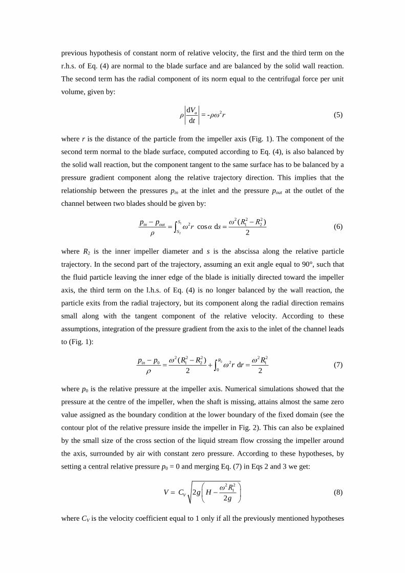
previous hypothesis of constant norm of relative velocity, the first and the third term on the

r.h.s. of Eq. (4) are normal to the blade surface and are balanced by the solid wall reaction.

The second term has the radial component of its norm equal to the centrifugal force per unit

volume, given by:

2d= -

d

aVρ ρω r

t (5)

where r is the distance of the particle from the impeller axis (Fig. 1). The component of the

second term normal to the blade surface, computed according to Eq. (4), is also balanced by

the solid wall reaction, but the component tangent to the same surface has to be balanced by a

pressure gradient component along the relative trajectory direction. This implies that the

relationship between the pressures pin at the inlet and the pressure pout at the outlet of the

channel between two blades should be given by:

1

2

2 2 22 1 2( )

cos d2

Sin out

S

p p ω R Rω r α s

ρ

(6)

where R2 is the inner impeller diameter and s is the abscissa along the relative particle

trajectory. In the second part of the trajectory, assuming an exit angle equal to 90°, such that

the fluid particle leaving the inner edge of the blade is initially directed toward the impeller

axis, the third term on the l.h.s. of Eq. (4) is no longer balanced by the wall reaction, the

particle exits from the radial trajectory, but its component along the radial direction remains

small along with the tangent component of the relative velocity. According to these

assumptions, integration of the pressure gradient from the axis to the inlet of the channel leads

to (Fig. 1):

2

2 2 2 2 220 1 2 1

0

( ) d

2 2

Rinp p R R R

r r

(7)

where p0 is the relative pressure at the impeller axis. Numerical simulations showed that the

pressure at the centre of the impeller, when the shaft is missing, attains almost the same zero

value assigned as the boundary condition at the lower boundary of the fixed domain (see the

contour plot of the relative pressure inside the impeller in Fig. 2). This can also be explained

by the small size of the cross section of the liquid stream flow crossing the impeller around

the axis, surrounded by air with constant zero pressure. According to these hypotheses, by

setting a central relative pressure p0 = 0 and merging Eq. (7) in Eqs 2 and 3 we get:

2 2

1 22

V

ω RV C g H

g

(8)

where CV is the velocity coefficient equal to 1 only if all the previously mentioned hypotheses

(steady-state conditions, radial symmetry and others) are exactly satisfied.

Experimental tests and numerical simulations were carried out in order to validate Eq.

(8) and to test the efficiency of the cross-flow turbine prototype designed by using the

procedure proposed in previous studies (Sammartano et al., 2013, 2014, 2015; Sinagra et al.,

2014). A second set of numerical simulations, using the commercial code ANSYS CFX, was

carried out in order to extend validation of Eq. (8) to other configurations of the CF turbine

within a large range of hydraulic head H, different number of blades Nb and various values of

the ratio between the inner radius R2 and the outer radius R1. This analysis gives important

hints for a better design of the CF turbine.

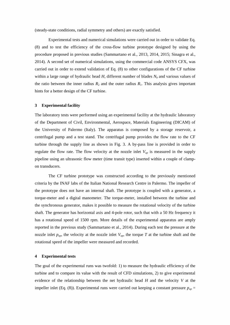
3 Experimental facility

The laboratory tests were performed using an experimental facility at the hydraulic laboratory

of the Department of Civil, Environmental, Aerospace, Materials Engineering (DICAM) of

the University of Palermo (Italy). The apparatus is composed by a storage reservoir, a

centrifugal pump and a test stand. The centrifugal pump provides the flow rate to the CF

turbine through the supply line as shown in Fig. 3. A by-pass line is provided in order to

regulate the flow rate. The flow velocity at the nozzle inlet Vup is measured in the supply

pipeline using an ultrasonic flow meter (time transit type) inserted within a couple of clamp-

on transducers.

The CF turbine prototype was constructed according to the previously mentioned

criteria by the INAF labs of the Italian National Research Centre in Palermo. The impeller of

the prototype does not have an internal shaft. The prototype is coupled with a generator, a

torque-meter and a digital manometer. The torque-meter, installed between the turbine and

the synchronous generator, makes it possible to measure the rotational velocity of the turbine

shaft. The generator has horizontal axis and 4-pole rotor, such that with a 50 Hz frequency it

has a rotational speed of 1500 rpm. More details of the experimental apparatus are amply

reported in the previous study (Sammartano et al., 2014). During each test the pressure at the

nozzle inlet pup, the velocity at the nozzle inlet Vup, the torque T at the turbine shaft and the

rotational speed of the impeller were measured and recorded.

4 Experimental tests

The goal of the experimental runs was twofold: 1) to measure the hydraulic efficiency of the

turbine and to compare its value with the result of CFD simulations, 2) to give experimental

evidence of the relationship between the net hydraulic head H and the velocity V at the

impeller inlet (Eq. (8)). Experimental runs were carried out keeping a constant pressure pup =

3922 Pa at the nozzle inlet section and exploring a wide range of rotating velocities, from 300

to 850 rpm. For each test the water discharge Q flowing into the turbine, the torque T of the

impeller external shaft and the rotational speed of the impeller were recorded.

The recorded variables were filtered in order to reduce the noise of the signal and to

remove the outlier values without losing the signal shape. First the data were de-noised by

means of the Fast Fourier Transform (FFT) algorithm (Frigo & Johnson, 1998); then the

outliers of the original data were removed using the whitening test of the residuals rs between

the original signal f and the smoothed one fs. Finally, the autocorrelation of the residuals

( rs , l ) was estimated in order to identify the data falling into a confidence interval of the

95% coverage with a fixed value of the lag time l (Brockwell & Davis, 1991):

1.96

( , ) l

ρ rs lN

(9)

where Nl is the number of observations. After the statistical analysis was performed on the

collected data series, the time averaged values of the velocity coefficient CV and of the turbine

efficiency η was estimated. The velocity coefficient CV was estimated using Eq. (8), while the

turbine efficiency η was calculated as follow:

(100)m

h

Pη

P (10)

where Pm is the average mechanical power measured at the external shaft and Ph is the

average hydraulic power lost inside the impeller. This power should be estimated as

difference between the inlet and outlet hydraulic power. However, because the hydraulic head

at the turbine outlet is usually negligible in both the real plants and in the tested prototype

with respect to the inlet hydraulic head the loss was estimated as:

2

2

up up

h

p VP γ Q

γ g

(11).

An error analysis was performed to evaluate the variability of the measured instantaneous

values, which is strongly related to the variability of the mean value. The standard error SEf of

the acquired signals was estimated assuming statistical independence of the sample values

(Everitt, 2003), and computed as the sample estimate σ f of the population standard deviation,

divided by the square root of the sample size n f:

f

f

f

σSE

n (12).

5 The simulation model

The results collected during the experiments were compared with the simulated ones.

Simulations were carried out using the Ansys CFX commercial code, solving the Reynolds-

averaged Navier Stokes (RANS) equations. CFX gives the option to select one of several

different turbulence models, and this choice is relevant for the output of the model. In this

analysis three two-equation turbulence models were considered as candidates: the k–ε model,

the RNG k–ε model and the Shear Stress Transport model (SST).

The k–ε turbulence model, as described in the study of Bardina, Huang, and Coakley

(1997), is useful for free-shear layer flows with relatively small pressure gradients. To model

the near wall region, where high pressure gradients occurred, the turbulence models based on

the ε-equation typically use the "Wall-Function Method" (Launder & Spalding, 1974; Viegas

& Rubesin, 1983; Viegas, Rubesin, & Horstman, 1985). This approach uses empirical laws to

circumvent the inability to predict a logarithmic velocity profile near the boundary walls. On

the other hand, when adverse pressure gradients occurs, turbulence models based on the ε–

equation lead to an overestimation of the turbulent length scale, resulting in high wall shear

stress in near-wall regions.

In order to avoid the use of wall-functions in the wall region and to allow integration

of the equations in the all flow domain, Wilcox (1993) introduced the k–ω turbulence model.

The ω–equation has significant advantages near the surface and accurately predicts turbulent

length scale in adverse pressure drops. The main deficiency of this model is the high

sensitivity of the solution in the free stream and the high computational demand. This

turbulence model, in the near wall region, uses the so-called "Low-Reynolds-Number"

approach (Jones & Launder, 1972), which resolves the details of the boundary layer using a

very small mesh length scale in the direction normal to the wall. Later on, to obtain a more

accurate calculation in regions with positive pressure gradient Menter (1993, 1994) proposed

the Shear Stress Transport (SST) turbulence formulation. The model applies the k-ε model in

the free shear flow and the k-ω model (Wilcox, 1993) in the inner region of the boundary

layer (Vieser, Esch, & Menter, 2003; Menter, Kuntz, & Langtry, 2003a).

A disadvantage of the two equation turbulent models is the excessive turbulence

levels in regions with large normal strain, like stagnation regions and regions with strong

acceleration. In order to avoid the build-up of turbulent kinetic energy in stagnation regions a

production limiter (Pk) can be used. In the present study the Kato-Launder modification (Kato

& Launder, 1993) was incorporated as production limiter in each of the investigated

turbulence models. This production limiter Pk has been proven to be useful to reduce

turbulence production in cases of very high acceleration and deceleration such as leading

edges, shocks and suction-side peaks (Kato & Launder, 1993; Senthooran, Dong-Dae, &

Parameswaran, 2004; Ansys Inc., 2012).

In the numerical simulations performed in this study the fluid domain was divided

into two physical sub-domains: the rotor (impeller) and the stator, made up of the nozzle and

the casing of the turbine. In the numerical simulations both water and air phases were

modelled according to the free surface homogeneous model, where the two species share the

same dynamic fields of pressure, velocity and turbulence (Ansys Inc., 2011, 2012). The

computational domain was discretized by a single 3D layer divided in tetrahedral and

prismatic elements. In both the k-ε model and the RNG k-ε model, the total number of

discretization elements was of about 800,000: 500,000 in the rotor domain and 300,000 in the

stator domain. In the test case of the SST model the grid density was increased close to the

boundary walls, particularly close to the blades and taking into account a dimensionless wall

distance y+ of about 80, as suggested in the analysis by Menter et al. (2003b). The total

number of discretization elements was about 1,700,000: 1,200,000 in the rotor domain and

500,000 in the stator domain. The boundary conditions selected in the simulations are: a) Inlet

boundary condition at the inlet section of the nozzle, with a water volume fraction equal to

one and all assigned velocity components, b) Opening boundary condition at the outlet

section of the casing, with a zero relative pressure, normal velocity to the boundary and a

water volume fraction equal to zero (Ansys Inc., 2011). The Opening boundary condition

means that both positive and negative fluxes are allowed for water and air.

In order to take into account the high pressure fluctuations and the unsteadiness due

to the rotation motion of the impeller, each of the RANS simulations was carried out in a

transient regime, as suggested in the study by Croquer, De Andrade, Clarembaux, Jeanty, and

Asuaje (2012). The frame change model used in each of the performed simulations was the

unsteady sliding grid approach, also called Transient Rotor-Stator approach in CFX (Ansys

Inc., 2011).

6 Experimental and numerical results

The error analysis, performed to estimate the error of each experimental data series, made it

possible to select the data series with the lowest standard error SEf and to discard the other

ones, in order to select only reliable values of efficiency η and of the velocity coefficient CV.

The experimental runs showed that the turbine designed with the procedure proposed in

previous studies (Sammartano et al., 2013, 2014, 2015; Sinagra et al., 2014) has an efficiency

always greater than 75% with an efficiency peak of 80.6% for a velocity ratio close to 2 (Vt/U

= 1.8), in agreement with the aforementioned design procedure and with Eq. (1). The

experimental efficiency curve is reported in Fig. 4, where the standard error SEf values for

each efficiency point are also shown. The experimental results were compared with the

numerical efficiency estimated by means of the CFD simulations, performed with three

different turbulence models.

The plot shows that the experimental efficiency of the designed turbine was always

greater than the numerical ones, but the SST turbulence model implemented with the Kato-

Launder production limiter (SST-KL) provides a better estimation of the turbine performance.

In order to better highlight the different reliability of the turbulence models the authors

reported in the Table 1 the error between the experimental results and the numerical

estimations calculated as follow:

* -= ×(100)

exp

eff

exp

η ηErr

η (13)

where η* is the estimated efficiency of the selected RANS model and ηexp is the experimental

one. The table clearly shows that the SST model seems to give the best fit among the others

models selected; the estimated error falls in a range between 0.05% and -1.55%.

In Figure 5 the velocity coefficient CV evaluated by means of Eq. (8), from recorded

experimental data as well as numerical simulations, is plotted against the velocity ratio. The

regression lines of both the experimental and simulated data sets provide an excellent

validation of Eq. (8), with a CV coefficient bounded by 0.95 and 1.0 for the numerical

simulations, by 0.9 and 0.95 for the experimental values and only weakly affected by the

actual velocity ratio. The linear regression of the estimated velocity coefficient is represented

by an almost horizontal line, although some spreading occurs; the regression coefficients are

R2 = 0.083 for the experimental values and R

2 = 0.065 for the numerical simulations. On the

other hand the estimation of the velocity coefficient by means of Eq. (8) does not seem to be

sensitive to the turbulence model implemented in the numerical simulations.

7 Validation of the velocity formula

Estimation of the velocity V at the impeller inlet by means of Eq. (8) does not take into

account the effect of some geometrical parameters, such as the number of blades Nb and the

diameter ratio D2/D1. These parameters obviously affect the shape of the channel between two

consecutive blades and this may affect the balance of the forces in the first term of Eq. (4), as

well as the estimation of the inlet pressure. The shape of the vane between two adjacent

blades can be described by the ratio Lc/Sc between the length Lc and the width Sc of the vane,

where Sc is measured along the mean circumference of the impeller (see the scheme of Fig.

1). A series of numerical simulations was carried out by means of ANSYS CFX solver in

order to extend the validation of the Eq. (8) to CF turbines designed with different

combinations of hydraulic head H, number of blades Nb and diameters ratio D2/D1. The

boundary conditions of the simulations and the adopted mesh are described in the previous

paragraph, while the SST KL (SST with the Kato-Launder limiter) model was selected in

order to get better results. The simulations were carried out by keeping the following design

parameters constant: the inlet attack angle ( = 22°), the impeller inlet angle (λ = 90°), the

rotational speed (ω = 757 rpm) and the velocity ratio Vt /U between the tangential inlet

velocity Vt and the velocity of the reference system.

Numerical solutions were carried out for five different H/D1 values (68.5, 75.0, 86.5,

96.6, 118.6), six blade numbers Nb (35, 40, 50, 60, 70, 80) and six different diameter ratios

D2/D1 (0.60, 0.65, 0.70, 0.75, 0.80, 0.85), for a total number of 180 simulations. For each

simulation run, the accuracy of Eq. (8) was tested by evaluating the relative error of the inlet

velocity estimation:

*

(100)vel

V VErr

V

(14)

where V* is the average velocity along the impeller inlet computed by the CFD solver and V is

the inlet velocity estimated by Eq. (8) with a velocity coefficient CV = 0.98. In Figure 6 the

error of the velocity estimation ERRvel is plotted versus the diameter ratio D2/D1 for each value

of the H/D1 parameter and for a number of blades Nb = 50; each point of the plot is associated

with the corresponding turbine efficiency. The plot shows that the diameter ratio D2/D1, and

hence the length of the vanes (Lc), strongly affects the turbine efficiency, as well as the water

head versus velocity relationship; moreover, higher values of efficiency can be observed

where lower values of the velocity estimation error occur (Errvel ≤ 5%). This correlation can

be explained by the additional energy losses occurring in sub-optimal turbines, which are

likely to provide a larger pressure at the impeller inlet, with respect to the one assumed in

deriving Eq. (8). This result is also a further validation of the design criterion previously

proposed by Sammartano et al. (2013), which is based on a reliable prediction of the inlet

average velocity. Finally, the plot shows that the value of the diameter ratio D2/D1 that

maximizes the turbine efficiency can always be found in the range between 0.75 and 0.80.

In order to select the number of blades Nb that maximizes the efficiency of the CF

turbine, for each value of the H/D1 parameter (H/D1 = 68.5, 75.0, 86.5, 96.6, 118.6), the

efficiency was estimated in the analyzed range of the diameter ratio D2/D1 and it was plotted

versus the dimensionless parameter Lc/Sc. In Figure 7 the family of curves relative to H/D1 =

68.5 is shown. In the plot the parameter of the efficiency curve is the number of blades Nb and

each point is associated to the corresponding diameter ratio D2/D1, printed to the side. The

plot shows that, for a fixed number of blades, the curves have a clear peak value and the

highest efficiency is attained for a diameter ratio between 0.75 and 0.80, in agreement with

the results observed in the previous plot (see Fig. 6). It can be observed, by interpolating the

efficiency peaks (ηmax) of each curve by means of a polynomial curve (in Fig. 7 the

interpolating curve is represented by the dotted line), that for this value of the parameter H/D1

the highest value of the efficiency occurs for Lc/Sc = 3.5. Carrying out a similar analysis for

each H/D1 parameter value, it is possible to plot a one-to-one relationship between the H/D1

and the Lc/Sc parameters holding at the optimum efficiency value. The five tested couples of

the two dimensionless parameters, H/D1 and Lc/Sc, are reported in Fig. 8. The results achieved

with the previous numerical study are summarized in the previous plot, which is helpful for a

preliminary design of the CF turbine, to be carried out without the help of CFD simulations.

Starting from the same geometrical parameters as used for the turbines analyzed in this study

(α = 22° and λ = 90°) and adopting a D2/D1 ratio equal to 0.75-0.80, we can do the following:

Estimate the outer diameter D1 by using Eqs 1 and 8, and the corresponding D2 value;

Enter in the plot in Fig. 8 with the relative H/D1 value to get the optimal Lc/Sc value;

Use the estimated Lc/Sc value to compute the optimal Nb number of blades.

The following equation can be used to compute the optimal number of blades:

1

1 2 ( )2

b

cb

c b

D Dπ w N

Lρ δ

S N

(15)

where b and are, respectively, the radius and the central angle of the blade, and w is the

width of the blade. The blade geometry (b and) can easily be estimated as reported in the

previous paper by Sammartano et al. (2013). The width of the blade should be set at the

minimum compatible with the structural needs of the blades and the maximum size of the

impeller.

8 Conclusions

The experimental and numerical work reported in this paper led to the validation and the

improvement of the design procedure of a CF turbine previously described in Sammartano et

al. (2013). The results of three different turbulence models were compared to select the best

one for the CF turbine simulations: the k–ε model, the RNG k–ε model and the Shear Stress

Transport model (SST). The results can be summarized as follows:

Experimental tests provide a good validation of the results obtained by means of CFD

analysis: the trends of the simulated and of the experimental efficiency curves are

similar, even if the experimental efficiency values are always a bit higher than the

simulated ones.

The SST turbulence model implemented with the Kato-Launder production limiter

provides a better estimation of the turbine performance.

The velocity coefficient CV, estimated by means of Eq. (8), is very close to 1 for all

experimental runs and it is almost independent from the velocity ratio. This means

that by evaluating the inlet velocity using Eq. (8) it is possible to perform a good

design of the turbine geometry, without iterating the same design according to the

actual relationship occurring between inlet velocity V and upstream head H.

A series of numerical simulations was carried out in order to get a numerical

validation of Eq. (8) also for CF turbines different from the experimental one. The

analysis was carried out using five different values of the dimensionless parameter

H/D1 and six possible values of the blade number Nb (Nb = 35, 40, 50, 60, 70, 80), as

well as of the diameter ratio D2/D1 (D2/D1 = 0.60, 0.65, 0.70, 0.75, 0.80, 0.85). The

analysis of the results showed that: 1) Eq. (8) provides very good inlet velocity

estimation, with an error smaller than 5%, when the turbine design follows the

efficiency optimality criterion proposed by Sammartano et al. (2013) and 2) the

highest efficiency occurs for a diameter ratio D2/D1 between 0.75 and 0.80. The

optimal Lc/Sc ratios were selected from the available numerical results for each of the

H/D1 investigated ratios. The parabolic curve obtained from these five points can be

useful for a preliminary design of the CF turbine, to select the number of blades Nb

obtained by the optimal Lc/Sc value corresponding to the given H/D1 ratio.

Notation

CT = velocity coefficient used when the relative pressure at the impeller inlet is zero, as

considered in the old velocity formula (Eq. (2)) (-)

CV = velocity coefficient in the authors' formula (Eq. (8)) (-)

D2/D1 = diameter ratio (-)

Erreff = error between the experimental results and the numerical estimations (%)

Errvel = relative error of the inlet velocity estimation (%)

f = time series of the measured data acquired during the experimental runs (Q(m3 s

-1),

T(s) and others)

fs = time series of the smoothed acquired data (Qs(m3 s

-1), Ts(s) and others)

f = inertial force per unit volume (N m-3

)

g = gravity acceleration (m s-²)

H = net head at the inlet of the nozzle (m)

l = lag time (s)

Lc = length of the vane between two adjacent blades (m)

Lc/Sc = shape factor of the vane between two adjacent blades (-)

n f = sample size of the collected data (-)

Nb = number of blades (-)

Nl = number of observations of each data series (-)

p = water relative pressure in the fluid domain (Pa)

p0 = water relative pressure at the impeller axis (Pa)

Ph = average hydraulic power lost inside the impeller (N m)

pin = water relative pressure at the impeller inlet (Pa)

Pk = production limiter of turbulent kinetic energy in stagnation regions (-)

Pm = average mechanical power measured at the external shaft (N m)

pout

= water relative pressure at the outlet of the channel between two blades (Pa)

pup = water relative pressure at the nozzle inlet (Pa)

Q = water discharge (m3 s

-1)

rs = residuals between the original signal f and the smoothed one fs

R2

= coefficient of regression (-)

R1 = impeller outer radius (m)

R2 = impeller inner diameter (m)

r = distance of the particle from the impeller axis (m)

s = curvilinear abscissa along the particle trajectory (m)

Sc = width of the vane between two adjacent blades (m)

S1 = inner abscissa along the trajectory (m)

S2 = outer abscissa along the trajectory (m)

SEf = standard error of the acquired signals (-)

T = torque at the turbine shaft (N m)

U = velocity of the reference system (m s-1

)

V = inlet impeller velocity (m s-1

)

V* = average velocity along the impeller inlet computed by the CFD solver (m s

-1)

Va = velocity of the reference system at the particle location (m s-1

)

Vr = relative velocity of the particle (m s-1

)

Vt = absolute tangential velocity (m s-1

)

Vt/U = velocity ratio (-)

Vup = absolute flow velocity at the nozzle inlet (m s-1

)

w = width of the blade (m)

y = wall distance (m)

y+

= dimensionless wall distance (-)

α = attack angle (°)

γ = water specific weight (N m-3

)

η = turbine efficiency (%)

η* = numerically estimated efficiency for a selected RANS model (%)

ηexp = experimental value of the turbine efficiency (%)

ηmax = the efficiency peaks in the curves for a fixed value of H/D1 and Nb (%)

λ = impeller inlet angle (°)

= water density (Kg m-3

)

( rs, l )= autocorrelation of the residuals rs(-)

σf = standard deviation of the acquired signal (-)

ω = rotational velocity of the impeller (rpm)

ω = vector normal to the trajectory plane and with norm equal to the rotational velocity

References

Ansys Inc. (2011). ANSYS CFX Solver Modeling Guide - r. 14. Southpointe 275 Technology

Drive Canonsburg, PA 15317.

Ansys Inc. (2012). ANSYS CFX Reference Guide. Southpointe, 275 Technology Drive

Canonsburg, PA 15317.

Aziz, N.M., & Desai, V.R. (1993). A Laboratory Study to Improve the Efficiency of Cross-

Flow Turbines (Engineering Report 1W-91). Department of Civil Engineering, Clemson

University, Clemson, SC, USA.

Bardina, J.E., Huang, P.G., & Coakley, T.J. (1997). Turbulence Modeling Validation, Testing,

and Development (NASA Technical Memorandum 110446). Ames Research Center,

Moffett Field, California 94035-1000.

Brockwell, P.J., & Davis, R.A. (1991). Time Series: Theory and Methods. Springer Series in

Statistics, Springer-Verlag, New-York.

Bruno, S.G., Choulot, A., & Denis, V., (2010). Energy Recovery in Existing Infrastructures

with Small Hydropower Plants. Brussels, Belgium: European Small Hydropower

Association.

Carravetta, A., Fecarotta, O., & Ramos, H. (2011). Numerical simulation on Pump As

Turbine: mesh reliability and performance concerns. Proceedings of IEEE (Ed.),

International Conference on Clean Electrical Power, Ischia, Franco Angeli Ed. Milano,

169-174.

Carravetta, A., Fecarotta, O., Del Giudice, G.,& Ramos, H. (2014). Energy recovery in water

systems by PATs: A comparisons among the different installation schemes. Procedia

Engineering, 70(2014), 275-284.

Chattha, J. A., Khan, M.S., Wasif, S.T., Ghani, O.A., Zia, M.O., & Hamid, Z. (2010, July).

Design of a cross flow turbine for a micro-hydro power application. Proceedingsof

ASME 2010 Power Conference, Chicago, Illinois, USA, July 13–15, 2010, 637-644,

Conference Sponsor: Power Division.

Crampes, C., & Moreaux, M. (2001). Water resource and power generation. International

Journal of Industrial Organization, 19(6), 975‐997.

Croquer, S. D., De Andrade, J.,Clarembaux, J., Jeanty, F., & Asuaje, M. (2012, June).

Numerical Investigation of a Banki Turbine in Transient State: Reaction Ratio

Determination. Proceedings of of ASME Turbo Expo 2012: Turbine Technical

Conference and Exposition Volume 8: Turbomachinery, Parts A, B, and C.

Copenhagen, Denmark, June 11–15, 2012. Conference Sponsor: International Gas

Turbine Institute.

De Andrade, J., Curiel, C., Kenyery, F., Aguilln, O., Vásquez, A., & Asuaje, M. (2011).

Numerical investigation of the internal flow in a Banki turbine. International Journal of

Rotating Machinery, Hindawi Publishing Corporation,Vol. 2011, Art.ID.841214, 12

pages.

Demirbas, A. (2007). Focus on the world: Status and future of hydropower. Energy Sources

Part B-Economics Planning and Policy, 2(3), 237-242.

Esch, T., Menter, F.R. &Vieser W. (2003, March). Heat transfer predictions based on two-

equation turbulence models. Proceedings of the 6th ASME-JSME Thermal Engineering

Joint Conference, March 16-20, 2003, Hawaii.

Everitt, B.S. (2003). The Cambridge Dictionary of Statistics. CUP. ISBN 0-521-81099-X.

Frigo, M. & Johnson, S. G. (1998). FFTW: An Adaptive Software Architecture for the FFT.

Proceedings of the International Conference on Acoustics, Speech, and Signal

Processing, Vol. 3, 1381-1384.

Gaius-Obaseki, T. (2010). Hydropower opportunities in the water industry. International

Journal of Environmental Science, 1(3), 392–402.

Jones, W. P. & Launder, B. E. (1972). The Prediction of Laminarization With a Two-

Equation Model of Turbulence. International Journalof Heat Transfer, 15, 301-314.

Jošt, D., Škerlavaj, A., & Lipej, A. (2014). Improvement of Efficiency Prediction for a

Kaplan Turbine with Advanced Turbulence Models. Journal of Mechanical

Engineering, 60(2014) 2, 124-134.

Kato, M., & Launder, B.E. (1993). The modelling of turbulent flow around stationary and

vibrating square cylinders. Proceedings of the9th Symposium on Turbulent Shear Flows,

Kyoto, Japan, August 16-18, 1993, Springer-Verlag Berlin Heidelberg New York.

Khurana, S., & Kumar, A. (2011). Small hydro power - A review. International Journal of

Thermal Technologies, 1(1), 107–110.

Kucukali, S. (2011). Water Supply Lines as a Source of Small Hydropower in Turkey: A

Case Study in Edremit. Linkӧping, Sweden. Proceedings of theWorld Renewable

Energy Congress, 8-13 May 2011, Linköping University Electronic Press, 1400.

Launder, B.E. & Spalding, D.B. (1974). The numerical computation of turbulent flows.

Computer Methods in Applied Mechanics and Engineering, 3, 269-289.

McNabola, A., Coughlan, P., Corcoran, L., Power, C., Williams, P. A., Harris, I., Gallagher,

J., & Styles, D. (2014). Energy recovery in the water industry using micro-hydropower:

an opportunity to improve sustainability. Water Policy, 16(2014), 168-183.

Menter, F. R. (1993). Zonal Two Equation k-ω Turbulence Models for Aerodynamic Flows.

AIAA Journal, 93-2906.

Menter, F. R., Carregal Ferreira, J., Esch, T. & Konno, B. (2003b). The SST Turbulence

Model with Improved Wall Treatment for Heat Transfer Predictions in Gas Turbines.

Proceedings of theInternational Gas Turbine Congress 2003 Tokyo, November 2-7,

IGTC 2003 Tokyo OS-202.

Menter, F. R., Kuntz, M., & Langtry, R., (2003a). Ten Years of Industrial Experience with the

SST Turbulence Model.Turbulence, Heat and Mass Transfer, eds. K. Hanjalic, Y.

Nagano, and M. Tummers, Begell House, Inc., 625 - 632.

Ramos, H., Mello, M., & De, P. (2010). Clean power in water supply systems as a sustainable

solution: From planning to practical implementation. Water Science and Technology,

10(1), 39-49.

Sammartano, V., Aricò, C., Carravetta, A., Fecarotta, O., & Tucciarelli, T. (2013). Banki-

Michell Optimal Design by Computational Fluid Dynamics Testing and Hydrodynamic

Analysis. Energies, 6(5), 2362-2385.

Sammartano, V., Aricò, C., Sinagra, M., & Tucciarelli, T. (2015). Cross-Flow Turbine Design

for Energy Production and Discharge Regulation. Journal of Hydraulic Engineering,

141(3), March 2015.

Sammartano, V., Morreale, G., Sinagra, M., Collura, A., & Tucciarelli, T. (2014).

Experimental study of Cross-Flow micro-turbines for aqueduct energy

recovery.Procedia Engineering, 89, 2014, 540-547.

Senthooran, S., Dong-Dae, Lee, & Parameswaran, S. (2004). A computational model to

calculate the flow-induced pressurefluctuations on buildings. Journal of Wind

Engineering and Industrial Aerodynamics, 92, 1131-1145.

Sinagra, M., Sammartano, V., Aricò, C., Collura, A., & Tucciarelli, T. (2014). Cross-Flow

turbine design for variable operating conditions. Procedia Engineering,70(2014), 1539–

1548.

Viegas, J. R. & Rubesin, M. W. (1983). Wall-Function Boundary Conditions in the Solution

of the Navier-Stokes Equations for Complex Compressible Flows. AIAA Journal, 83-

1694.

Viegas, J. R., Rubesin, M. W., & Horstman, C. C. (1985). On the Use of Wall Functions as

Boundary Conditions for Two-Dimensional Separated Compressible Flows. AIAA

Journal, 85-0180,

Vieser, W., Esch, T. & Menter, F. (2003). Heat Transfer Predictions using Advanced Two

Equation Turbulence Models. CFX Technical Memorandum, CFX-VAL10/0602, date of

publication 11/06/2002, Unlimited Distribution.

Wilcox, D. C. (1993). Comparison of two-equation turbulence models for boundary layers

with pressure gradient, AIAA Journal, Volume 31(8), 1414-1421.

Wilcox, D. C. (1998). Turbulence Modeling for CFD. Second edition. Anaheim: DCW

Industries, 162-165.

Williams, A.A., & Simpson, R. (2009). Pico hydro – Reducing technical risks for rural

electrification. Renewable Energy, 34, 1986-1991.

Yakhot, V., Orszag, S.A., Thangam, S., Gatski, T.B. & Speziale, C.G. (1992). Development

of turbulence models for shear flows by a double expansion technique. Physics of

FluidsA, 4(7),1510-1520.

Yang, X., Song, Y., Wang ,G., & Wang, W. (2010). A Comprehensive Review on the

Development of Sustainable Energy Strategy and Implementation in China. IEEE

Transactions on Sustainable Energy, 1, 57-65.

Zanette, J., Imbault, D., & Tourabi, A. (2010). A design methodology for cross flow water

turbines. Renewable Energy, 35(2010), 997-1009.

Zia, O., Ghani, O.A., Wasif, S.T., & Hamid, Z., (2010). Design, fabrication and installation of

a micro-hydro power plant. Report of the Faculty of Mechanical Engineering GIK

Institute of Engineering Sciences & Technology Pakistan.

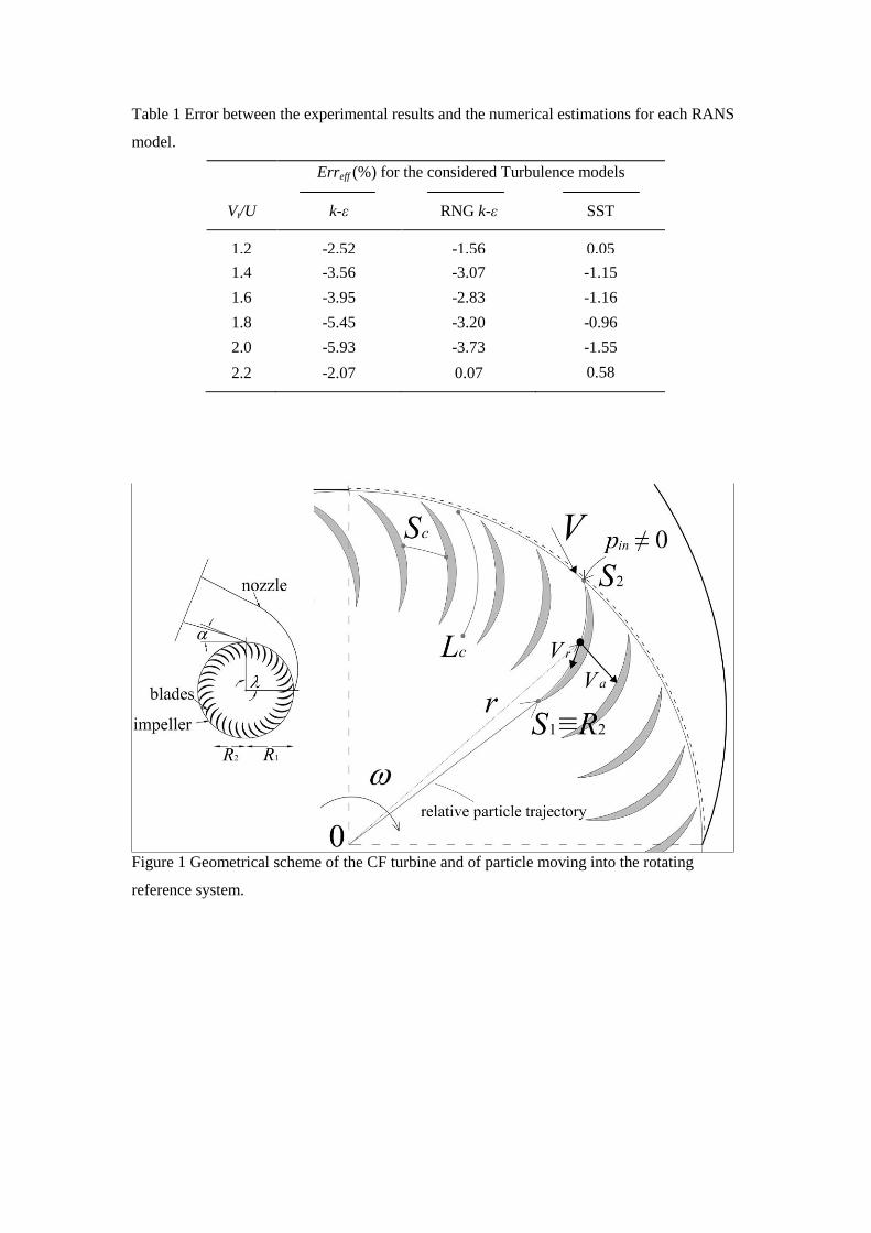
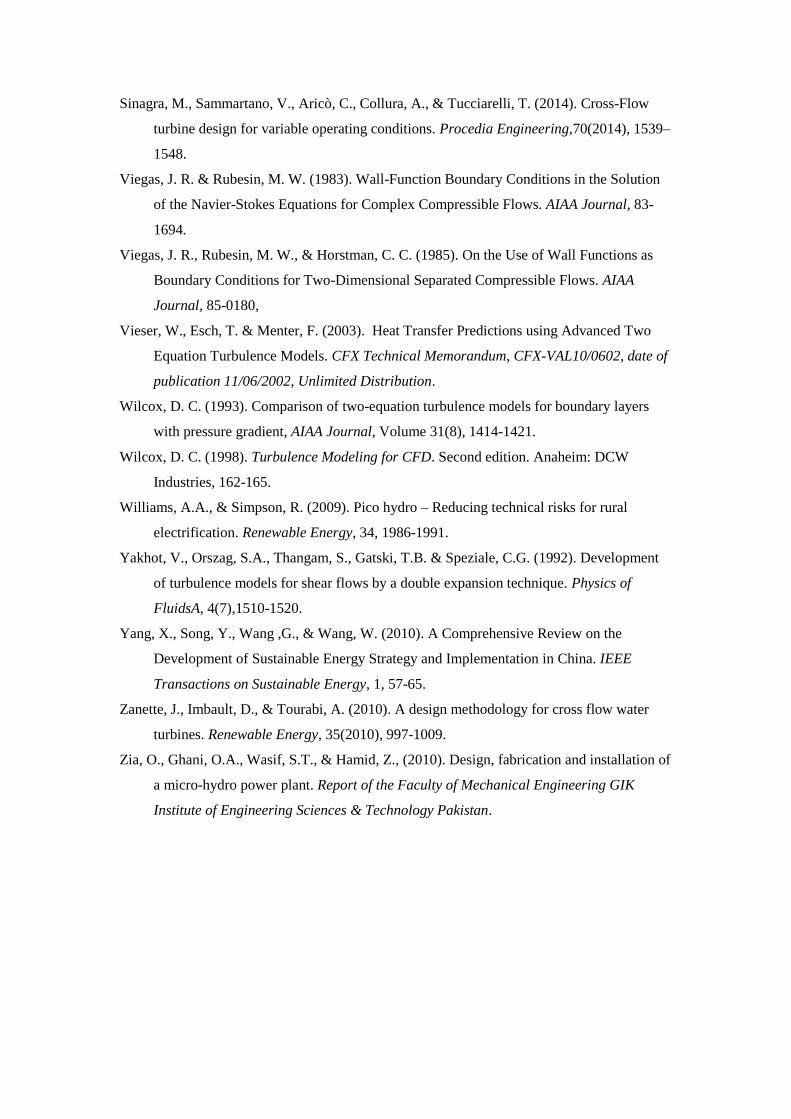
Table 1 Error between the experimental results and the numerical estimations for each RANS

model.

Vt/U

Erreff (%) for the considered Turbulence models

k-ε RNG k-ε SST

1.2 -2.52 -1.56 0.05

1.4 -3.56 -3.07 -1.15

1.6 -3.95 -2.83 -1.16

1.8 -5.45 -3.20 -0.96

2.0 -5.93 -3.73 -1.55

2.2 -2.07 0.07 0.58

Figure 1 Geometrical scheme of the CF turbine and of particle moving into the rotating

reference system.

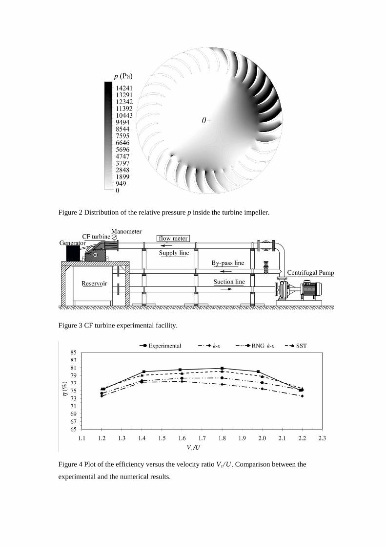
Figure 2 Distribution of the relative pressure p inside the turbine impeller.

Figure 3 CF turbine experimental facility.

Figure 4 Plot of the efficiency versus the velocity ratio V t /U . Comparison between the

experimental and the numerical results.

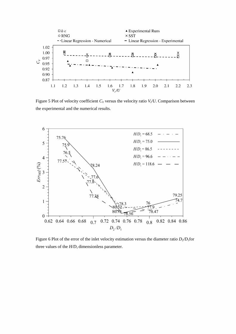
Figure 5 Plot of velocity coefficient CV versus the velocity ratio Vt/U. Comparison between

the experimental and the numerical results.

Figure 6 Plot of the error of the inlet velocity estimation versus the diameter ratio D2/D1for

three values of the H/D1 dimensionless parameter.

Figure7 Family of curves for H/D1= 68.5.

Figure 8 Relationship between the dimensionless parameters H/D1 and Lc/Sc.