numerical and experimental study of a boosted uniflow 2 ... · numerical and experimental study of...
TRANSCRIPT
Numerical and Experimental Study of a Boosted Uniflow 2-Stroke Engine
A thesis submitted for the degree of Doctor of
Philosophy
by
Jun Ma
Department of Mechanical, Aerospace and Civil Engineering
College of Engineering, Design and Physical Sciences
Brunel University London
September 2014

I
Abstract
Engine downsizing is one of the most effective ways to reduce vehicle fuel
consumption. Highly downsized (>50%) 4-stroke gasoline engines are constrained
by knocking combustion, thermal and mechanical limits as well as high boost.
Therefore a research work for a highly downsized uniflow 2-stroke engine has been
proposed and carried out to unveil its potential.
In this study, one-dimensional (1D) engine simulation and three-dimensional (3D)
computational fluid dynamic analysis were used to predict the performance of a
boosted uniflow 2-stroke DI gasoline engine. This was experimentally complemented
by the in-cylinder flow and mixture formation measurements in a newly
commissioned single cylinder uniflow 2-stroke DI gasoline engine.
The 3D simulation was used to assess the effects of engine configurations for engine
breathing performance and in order that the design of the intake ports could be
optimised. The boundary conditions for 1D engine simulation were configured by the
3D simulation output parameters, was employed to predict the engine performance
with different boost systems. The fuel consumption and full load performance data
from the 1D engine simulation were then included in the vehicle driving cycle
analysis so that the vehicle performance and fuel consumption over the NEDC could
be obtained.
Based on the modelling results, a single cylinder uniflow 2-stroke engine was
commissioned by incorporating a newly designed intake block and modified intake
and exhaust systems. In-cylinder flow and fuel distribution were then measured by
means of Particle Image Velocimetry (PIV) and Planar Laser Induced Fluorescence
(PLIF) in the single cylinder engine.
The numerical analysis results suggested that a 0.6 litre two-cylinder boosted uniflow
2-stroke engine with an optimised boosting system was capable of delivering
comparable performance to a NA 1.6 litre four-cylinder 4-stroke engine yet with a
maximum 23.5% improvement potential on fuel economy. Furthermore, simulation

II
results on in-cylinder flow structure and fuel distribution were then verified
experimentally.

III
Acknowledgments
First of all, I would like to express my sincere gratitude to my supervisor, Professor
Hua Zhao and Professor Alasdair Cairns for their unlimited support and guidance
throughout the work.
Also, I would like to give my deepest thanks to Mr Quan Liu, Mr Kangwoo Seo, Dr
Yan Zhang and Dr Cho-Yu Li for their help throughout my time at Brunel University.
And I would like to thank the technicians Mr Andrew Selway, Mr Kenneth Anistiss
and Mr Clive Barratt for the guidance and support in the laboratory.
Last but not least, I would like to thank my parents and my wife Lei Wang for their
unconditional support.

IV
Nomenclature
Abbreviations
ATDC After Top Dead Centre
BDC Bottom Dead Centre
BDD Blow-Down Duration
BR Burnt Rate
BSFC Brake Specific Fuel Consumption
BTDC Before Top Dead Centre
BUSDIG Boosted Uniflow Scavenged Direct Injection Gasoline
CA Crank Angle
CAI Controlled Auto Ignition
CCD Charge Coupled Device
CE Charging Efficiency
CFD Computational Fluid Dynamics
DAQ Data Acquisition
DCA Degree Crank Angle
DEV Duration of Exhaust Valves Opening
DI Direct Injection
DIATA Direct Injection Aluminium Through-Bolt Assembly
DISI Direct Injection Spark Ignition
DPM Discrete Phase Model
V
DR Delivery ratio
EGR Exhaust Gas Recirculation
EVC Exhaust Valve Closing
EVO Exhaust Valve Opening
FMEP Friction Mean Effective Pressure
FTP Federal Test Procedure
GDI Gasoline Direct Injection
HWA Hot Wire Anemometry
IA Interrogation Area
IMEP Indicated Mean Effective Pressure
IPC Intake Port Closing
IPO Intake Port Opening
LDA/LDV Doppler Anemometry/Velocimetry
LES Large-eddy Simulation
LIEF Laser Induced Exciplex Fluorescence
LIF Laser-Induced Fluorescence
LRS Laser Rayleigh Scattering
MBF Mass of Burned Fraction
NA Natural Aspirated
NEDC New European Drive Cycle
PFI Port fuel injection
PIV Particle image velocimetry

VI
PLIF Planar Laser-Induced Fluorescence
PTV Particle Tracking Velocimetry
RANS Reynolds-Averaged Navier-Stokes
SE Scavenging Efficiency
SI Spark Ignition
SMD Sauter Mean Diameter
SOI Start of Injection
SRS Spontaneous Raman Scattering
TDC Top Dead Centre
TE Trapping Efficiency
TTL Transistor–Transistor Logic
VCT Variable Cam Timing
VVT Variable Valve Timing
WOT Wide Opening Throttle

VII
Symbols in Roman
A engine stroke
AE effective area of intake port
Aeff effective area of the valve
Afront vehicle frontal area
Ai axis inclination angle
Aj area at the cell centre
Ap intake port area along the cylinder wall
BSR* blade speed ratio
Cdrag aerodynamic drag coefficient
Cf flow coefficient
Cht heat transfer multiplier constant
CoVcyc
deviation of the mean light intensity to the ensemble average
value
CoVf
deviation of the light intensity at each pixel from the mean light
intensity
Cp specific heat of the gas
Cpb port width ratio
Croll tyre rolling resistance factor
Cwb exponent in Wiebe function
D valve reference diameter
Dref reference diameter

VIII
d feature diameter of pipe wall
E total energy
Ev spectral fluence of the laser
force vector
Fdrag drag force
Froll tyre rolling resistance force
f lens focal length
H angular momentum
h enthalpy
he elevation of the point above a reference plane
Gb generation of turbulence kinetic energy due to buoyancy
Gk generation of turbulence kinetic energy due to the mean
velocity gradients
gravitational acceleration
I momentum inertia
Ii light intensity of each pixel
Imean
mean light intensity of all pixels in the region of interest of each
frame
Imean,cyc mean light intensity of all frames taken with same condition
Iv laser spectral intensity
diffusion flux
k turbulence kinetic energy
ke conductivity of the wall

IX
keff effective conductivity
L valve lift
m mass flow
mload passenger and cargo mass
mveh vehicle mass
dimensionless mass flow
N number of ports
N* dimensionless speed
Nr rotational speed
PR pressure Ratio
Pr prandtl number
Δp pressure drop along the pipe
p pressure
pcyl peak in-cylinder pressure
ps piston location from TDC at specified crank angle
Q heat transfer between pipe wall and inner gas
R resistivity of the absorptive material
RE effective ratio of area
Re Reynolds number
Rg gas constant
location vector
rcy engine bore

X
rp radius of swirl circle
S swirl ratio
Sh heat of chemical reaction, and any other volumetric heat
sources
Sm mass added to the continuous phase from the dispersed
second phase
SAwall wall surface area
T temperature
Tcb combustion duration
Tgas inner gas temperature
Tt engine Torque
Twall wall temperature
t time
Δt time interval
Uj velocity at the cell centre
ui fluid velocity
v fluid kinematic viscosity
velocity vector
Wc power consumed by the compressor
Wt power generated by the turbine
Δx length of the cell
element displacement
xb effective port shoulder width

XI
xp effective port width
YM contribution of the fluctuating dilatation in compressible
turbulence to the overall dissipation rate

XII
Symbols in Greek
Γ* dimensionless torque coefficient
Ψ state of the particle ensemble
Ω collection solid angle
γ special heat capacity ratio
ε turbulence dissipation rate
θ degrees past start of combustion
θb port shoulder width angle
θc crank angle
θp port width angle
η transmission efficiency of the collection optics
ρ density
τ Shaft torque
stress tensor
φp swirl orientation angle
ω0 crank shaft angular velocity

XIII
Contents
Abstract ....................................................................................................................... I
Acknowledgments ..................................................................................................... III
Nomenclature ............................................................................................................ IV
Abbreviations ......................................................................................................... IV
Symbols in Roman ................................................................................................ VII
Symbols in Greek .................................................................................................. XII
Contents .................................................................................................................. XIII
List of Figures ....................................................................................................... XVIII
List of Tables ........................................................................................................ XXIV
Chapter 1 Introduction ............................................................................................ 1
1.1 Introduction ....................................................................................................... 1
1.2 Objectives ......................................................................................................... 2
1.3 Outline of thesis ................................................................................................ 3
Chapter 2 Literature Review ................................................................................... 5
2.1 Introduction ....................................................................................................... 5
2.2 Advanced engine technologies ......................................................................... 6
2.3 Engine downsizing and boosting technologies .................................................. 7
2.4 2-stroke engines ............................................................................................. 11
2.4.1 Scavenging methods of the 2-stroke engine ............................................. 11
2.4.2 Previous research on uniflow 2-stroke engines ........................................ 13
2.5 In-cylinder flow measurements ....................................................................... 16
2.6 In-cylinder fuel distribution .............................................................................. 18
2.7 Summary ......................................................................................................... 20
Chapter 3 Analytical studies of flow and mixing in a uniflow 2-stroke engine ....... 22
3.1 Introduction ..................................................................................................... 22

XIV
3.1.1 Introduction to CFD simulation .................................................................. 23
3.1.2 Turbulence model ..................................................................................... 23
3.2 CFD Model Set-Up .......................................................................................... 26
3.2.1 Principle of Simulation .............................................................................. 27
3.2.2 Boundary Conditions ................................................................................ 29
3.2.3 Grid and Mesh Types ............................................................................... 30
3.3 CFD Calculation with 2D Model ...................................................................... 33
3.3.1 2D Model Design ...................................................................................... 34
3.3.2 2D Model simulation and results ............................................................... 39
3.4 3D CFD Calculations ...................................................................................... 43
3.4.1 3D CFD engine model .............................................................................. 43
3.4.2 3D CFD simulation results ........................................................................ 45
3.5 Fuel injection and in-cylinder mixing ............................................................... 53
3.5.1 Single injection .......................................................................................... 55
3.5.2 Split Injections ........................................................................................... 56
3.6 Summary ......................................................................................................... 58
Chapter 4 Prediction of the Uniflow 2-Stroke Engine Performance ...................... 60
4.1 Introduction ..................................................................................................... 60
4.2 1D Engine Model Setup .................................................................................. 61
4.3 1D Engine Simulation Results ......................................................................... 71
4.3.1 Effect of Engine Geometry on Performance ............................................. 72
4.3.2 Effect of the Blow-down Duration .............................................................. 76
4.3.3 Engine Packaging ..................................................................................... 81
4.4 Summary ......................................................................................................... 83
Chapter 5 Optimisation of the Boost System for the Uniflow 2-Stroke Engine ..... 84
5.1 Introduction ..................................................................................................... 84
5.2 Modelling of the Boosted Engine and Vehicle Simulation Model .................... 84

XV
5.3 Analysis of Boosted uniflow 2-stroke engine operations ................................. 89
5.3.1 2-stroke engine model set up .................................................................... 91
5.3.2 Prediction of Boosted uniflow 2-stroke engine full-load performance ....... 95
5.3.3 Analysis of boosted uniflow 2-stroke engine operations ......................... 102
5.3.4 2 Vehicle simulation results based on New European Driving Cycle
(NEDC) ............................................................................................................ 118
5.4 Summary ....................................................................................................... 122
Chapter 6 Single Cylinder Uniflow 2-stroke Engine and Experimental Facility .... 123
6.1 Introduction ................................................................................................... 123
6.2 Uniflow 2-stroke engine setup ....................................................................... 123
6.2.1 Cylinder Head ......................................................................................... 125
6.2.2 Optical window ring ................................................................................. 126
6.2.3 Cylinder liner ........................................................................................... 127
6.2.4 Intake port block and intake channel block ............................................. 128
6.2.5 Piston assembly ...................................................................................... 130
6.2.6 Timing belt mounting .............................................................................. 131
6.3 Boosted air intake system ............................................................................. 132
6.4 Fuel supply system ....................................................................................... 134
6.5 Spark ignition system and Timing Unit .......................................................... 137
6.6 In-cylinder pressure and heat release analysis ............................................. 138
6.7 Summary ....................................................................................................... 139
Chapter 7 In-Cylinder Flow Measurements with PIV .......................................... 140
7.1 Introduction ................................................................................................... 140
7.2 Experimental setup of PIV ............................................................................. 142
7.2.1 Flow seeding ........................................................................................... 142
7.2.2 PIV Laser ................................................................................................ 143
7.2.2 Camera and Optics ................................................................................. 144

XVI
7.2.3 PIV test setup ......................................................................................... 144
7.3 Evaluation of the particle displacement vector .............................................. 147
7.4 Results of PIV test ........................................................................................ 151
7.4.1 In-cylinder flow structure on the horizontal plane @ 600rpm engine speed
......................................................................................................................... 151
7.4.2 In-cylinder flow structure on the horizontal plane @ 900rpm engine speed
......................................................................................................................... 158
7.5 Summary ....................................................................................................... 162
Chapter 8 In-Cylinder Measurements of Fuel Distribution and Flame Propagation
in the Uniflow 2-stroke Engine ................................................................................ 163
8.1 Introduction ................................................................................................... 163
8.2 Principle of the PLIF Technique .................................................................... 163
8.3 PILF experimental setup ............................................................................... 166
8.4 Results of PLIF measurements ..................................................................... 168
8.4.1 Fuel Injection characteristics ................................................................... 168
8.4.2 Fuel distribution at 15°CA BTDC ............................................................ 172
8.4.3 Fuel distribution at 15°CA BTDC and SOI 120°CA BTDC ...................... 180
8.5 Combustion Studies ...................................................................................... 182
8.6 Summary ....................................................................................................... 187
Chapter 9 Conclusions and Recommendations for Future Work ........................ 189
9.1 Introduction ................................................................................................... 189
9.2 Design of intake ports ................................................................................... 189
9.3 In-cylinder fuel distribution ............................................................................ 190
9.4 Uniflow engine geometry and scavenging timings ........................................ 191
9.5 The boosted uniflow 2-stroke powertrain and its application to a vehicle ...... 191
9.6 Single cylinder uniflow 2-stroke engine and its in-cylinder flow and fuel
distributions ......................................................................................................... 192
9.7 Recommendations for future work ................................................................ 193

XVII
9.7.1 Engine simulations ..................................................................................... 193
9.7.2 In-cylinder flow and fuel distribution measurements .................................. 194
9.7.3 Engine thermal and emission performance ................................................ 194
References ............................................................................................................. 195
Appendix ................................................................................................................ 203

XVIII
List of Figures
Figure 2.1 Comparison of global regulations for passenger cars [1] .......................... 5
Figure 2.2 Limits of engine boosted by supercharger and turbocharger .................. 10
Figure 2.3 Typical 2-stroke engine scavenging methods ......................................... 12
Figure 2.4 Full-load performance of loop-flow and uniflow 2-stroke engine ............. 14
Figure 2.5 In-cylinder flow structure ......................................................................... 15
Figure 3.1 Typical Grid Shapes ................................................................................ 32
Figure 3.2 The intake port geometry parameter ....................................................... 33
Figure 3.3 The 2D CFD model ................................................................................. 35
Figure 3.4 Boundary of exhaust valves .................................................................... 36
Figure 3.5 Boundary of valve dynamic zones and clearance volume zone .............. 37
Figure 3.6 Boundary of swept volume ...................................................................... 38
Figure 3.7 Boundary of intake port channel .............................................................. 38
Figure 3.8 In-cylinder components distribution contour ............................................ 40
Figure 3.9 Engine scavenging performance as a function of axis inclination angle
based on 2D models ................................................................................................ 41
Figure 3.10 Effective area ratio of intake port ........................................................... 42
Figure 3.11 3-D CFD base model ............................................................................ 43
Figure 3.12 Valve zone, valve dynamic zone and clearance volume ....................... 44
Figure 3.13 Intake port channel layout ..................................................................... 45
Figure 3.14 Engine breathing performance as a function of axis inclination angle
based on 3D models ................................................................................................ 46
Figure 3.15 In-cylinder velocity vector ...................................................................... 49
Figure 3.16 Mass flow rate of intake ports and swirl ratio ......................................... 50
Figure 3.17 In-cylinder flow field .............................................................................. 50
Figure 3.18 Delivery ratio and port width ratio .......................................................... 52
Figure 3.19 Swirl ratio vs. swirl orientation angle ..................................................... 52
Figure 3.20 Scavenging performance vs. swirl orientation angle ............................. 53
Figure 3.21 DI injector geometry .............................................................................. 54
Figure 3.22 Mass of Evaporated Fuel ...................................................................... 55
Figure 3.23 The liquid fuel distribution...................................................................... 56
Figure 3.24 Liquid fuel location against radial coordination of CFD model ............... 56

XIX
Figure 3.25 Injection Timing Sequence .................................................................... 57
Figure 3.26 Injection Timing Sequence .................................................................... 57
Figure 3.27 Mass of Evaporated Fuel ...................................................................... 58
Figure 3.28 Liquid Fuel Volume ............................................................................... 58
Figure 3.29 Liquid Droplet Number .......................................................................... 58
Figure 4.1 Baseline 1D engine models ..................................................................... 62
Figure 4.2 Throttle element structure ....................................................................... 64
Figure 4.3 Base valve lift profile of uniflow 2-stroke engine model ........................... 66
Figure 4.4 Valve flow coefficient of uniflow 2-stroke model ..................................... 66
Figure 4.5 Scavenge profile ..................................................................................... 68
Figure 4.6 Gas-exchange performance of 3D and 1D models ................................. 69
Figure 4.7 FMEP calibration of 2-stroke engine model ............................................ 71
Figure 4.8 The timing sequence of 2-stroke operation ............................................. 72
Figure 4.9 Delivery ratio at IPO – 90°ATDC , BDD – 60°CA ................................... 73
Figure 4.10 Trapping efficiency at IPO – 90°ATDC , BDD – 60°CA ......................... 73
Figure 4.11 Charging efficiency at IPO – 90°ATDC , BDD – 60°CA ......................... 74
Figure 4.12 Specific indicated power at IPO – 90°ATDC , BDD – 60°CA, CA50 - 15º
ATDC ....................................................................................................................... 74
Figure 4.13 Specific indicated power at IPO – 90°ATDC , BDD – 60°CA, CA50 - 5º
ATDC ....................................................................................................................... 75
Figure 4.14 Specific indicated power at IPO – 90°ATDC , BDD – 60°CA, CA50 - 5º
ATDC ....................................................................................................................... 76
Figure 4.15 Intake port opening - 110°ATDC ........................................................... 77
Figure 4.16 Intake port opening – 120°ATDC .......................................................... 77
Figure 4.17 Intake port opening - 130°ATDC ........................................................... 78
Figure 4.18 In-Cylinder Peak Pressure .................................................................... 79
Figure 4.19 Specific indicated power output at 4000rpm, 3 bar boost, and CA50 at
15 CA ATDC ............................................................................................................ 80
Figure 4.20 Effect of blowdown duration on specific brake power output with 3 bar
boost ........................................................................................................................ 80
Figure 4.21 Vehicle application packaging restrictions ............................................. 82
Figure 4.22 Engine size determination ..................................................................... 82
Figure 5.1 Boost elements map extrapolation .......................................................... 86
Figure 5.2 The new Europe drive-cycle (NEDC) conditions ..................................... 89

XX
Figure 5.3 Valve timing and lift of 4-stroke baseline model ...................................... 90
Figure 5.4 Combustion phase of the 4-stroke engine model .................................... 90
Figure 5.5 Baseline engine model performance curve ............................................. 91
Figure 5.6 2-stroke 1D calculation base model layout .............................................. 92
Figure 5.7 Eaton R200GT performance map ........................................................... 93
Figure 5.8 Eaton R410GT performance map ........................................................... 94
Figure 5.9 Rescaled turbine performance map ........................................................ 94
Figure 5.10 Rescaled compressor performance map............................................... 95
Figure 5.11 Full load brake power of engine model with R200GT supercharger at
4000rpm engine speed. ............................................................................................ 96
Figure 5.12 R200GT supercharger working points at engine full load at 4000 rpm
engine speed ............................................................................................................ 96
Figure 5.13 Power consumption by a R200GT supercharger and the proportion to
the engine indicated power at 4000rpm full load operation ...................................... 97
Figure 5.14 Full load brake power of engine model with a R410GT supercharger at
4000rpm engine speed. ............................................................................................ 97
Figure 5.15 R410GT supercharger working points at engine full load at 4000 rpm
engine speed ............................................................................................................ 98
Figure 5.16 Power consumption by R410GT supercharger and the proportion to the
engine indicated power at 4000rpm full load condition ............................................. 98
Figure 5.17 Working points of the compressor and turbine of the model ............... 100
Figure 5.18 Full load power and torque curves of the turbocharged model ............ 101
Figure 5.19 Full load brake power and torque curves of all engines ..................... 102
Figure 5.20 Charging efficiency of baseline 4-stroke and boosted 2-stroke engines
............................................................................................................................... 103
Figure 5.21 IMEP values at 4000rpm and 55kW .................................................... 104
Figure 5.22 Intake and exhaust pressures at 4000rpm and 55kW ......................... 104
Figure 5.23 Residual Gas Fraction at 4000rpm and 55kW ..................................... 105
Figure 5.24 Engine output breakdown analysis at 4000rpm and 55kW.................. 106
Figure 5.25 BSFC at 4000rpm and 55kW .............................................................. 106
Figure 5.26 Charging efficiency at 4000rpm and 35kW.......................................... 107
Figure 5.27 IMEP at 4000rpm and 35kW ............................................................... 107
Figure 5.28 Intake and exhaust pressures at 4000rpm and 35kW ......................... 108
Figure 5.29 Residual Gas Fraction at 4000rpm and 35kW ..................................... 108
XXI
Figure 5.30 Engine output breakdown analysis at 4000rpm and 35kW................. 109
Figure 5.31 BSFC at 4000rpm and 35kW .............................................................. 109
Figure 5.32 Engine output breakdown analysis at 4000rpm and 10kW.................. 110
Figure 5.33 BSFC at 4000rpm and 10kW .............................................................. 110
Figure 5.34 Engine output breakdown analysis at 2000rpm, 20kW ....................... 111
Figure 5.35 Engine output breakdown analysis at 2000rpm, 10kW ....................... 111
Figure 5.36 Engine output breakdown analysis at 2000rpm, 6kW ......................... 112
Figure 5.37 Engine output breakdown analysis at 1000rpm, 10kW ....................... 112
Figure 5.38 Engine output breakdown analysis at 1000rpm, 5kW ......................... 113
Figure 5.39 BSFC comparisons at the same speed and load conditions between 4-
stroke engine and 2-stroke engines ....................................................................... 113
Figure 5.40 BSFC at various engine speed and load. ............................................ 114
Figure 5.41 Full load brake power and torque of turbocharged 2-stroke engines .. 115
Figure 5.42 BSFC of the baseline 4-stroke and turbocharged 2-stroke engines at the
same speed and power .......................................................................................... 116
Figure 5.43 BSFC of the baseline 4-stroke and downspeeded 2-stroke engines ... 116
Figure 5.44 BSFC contours of the 4-stroke and turbocharged 2-stroke engines .... 117
Figure 5.45 BSFC contours of the turbocharged 2-stroke engines and the rescaled
BSFC map of the baseline 4-stroke engine ............................................................ 118
Figure 5.46 Engine operating points with gear set1 during NEDC and engine full load
torque curves ......................................................................................................... 119
Figure 5.47 Engine operating points with gear set2 during NEDC and engine full load
torque curves ......................................................................................................... 120
Figure 5.48 Engine operating points with gear set2 during NEDC and engine full load
torque curves ......................................................................................................... 121
Figure 5.49 Average fuel consumption over NEDC ................................................ 122
Figure 6.1 Uniflow 2-Stroke Single Cylinder Engine assembly layout .................... 124
Figure 6.2 Cylinder head layout ............................................................................. 126
Figure 6.3 Optical window ring ............................................................................... 127
Figure 6.4 New Cylinder Liner ................................................................................ 128
Figure 6.5 Intake port block and intake channel block layout ................................. 129
Figure 6.6 Intake port block configuration .............................................................. 130
Figure 6.7 Intake channel block configuration ........................................................ 130
Figure 6.8 Piston assembly .................................................................................... 131

XXII
Figure 6.9 Camshaft pulley and crankshaft pulley for 2-strok operation ................. 132
Figure 6.10 The intake system layout..................................................................... 133
Figure 6.11 The intake and exhaust layout in the single cylinder engine ............... 134
Figure 6.12 Fuel supply system layout ................................................................... 135
Figure 6.13 Fuel tank, air driven pump and fuel rail ............................................... 136
Figure 6.14 Air Pump performance curve ............................................................... 136
Figure 6.15 Spark ignition control system .............................................................. 137
Figure 6.16 Timing sequence for fuel injection and image acquisition ................... 138
Figure 7.1 Typical PIV experimental setup ............................................................. 141
Figure 7.2 Straddling technique ............................................................................. 141
Figure 7.3 Flow seeding generator ......................................................................... 142
Figure 7.4 PIV test layout ....................................................................................... 145
Figure 7.5 Laser lining setup .................................................................................. 145
Figure 7.6 Illumination laser level position .............................................................. 146
Figure 7.7 Adjusting camera focus with an assisting subject ................................. 147
Figure 7.8 Averaged flow structure @90ºCABTDC ................................................ 151
Figure 7.9 Averaged flow structure @60ºCABTDC ................................................ 152
Figure 7.10 CFD simulation results of in-cylinder flow structure on the horizontal and
vertical plane @60ºCABTDC ................................................................................. 153
Figure 7.11 Averaged flow structure @30ºCABTDC .............................................. 154
Figure 7.12 Measured and flow fields with 1.2bar pressure ................................. 155
Figure 7.13 Average velocity of the region of interest ............................................ 157
Figure 7.14 Averaged flow structure @90ºCABTDC .............................................. 158
Figure 7.15 Averaged flow structure @60ºCABTDC .............................................. 159
Figure 7.16 Averaged flow structure @30ºCABTDC .............................................. 160
Figure 7.17 Average velocity across the region of interest on the horizontal plane 161
Figure 7.18 Swirl ratio across the region of interest on the horizontal plane .......... 161
Figure 8.1 Energy level diagram of LIF .................................................................. 164
Figure 8.2 Laser beam delivery system .................................................................. 167
Figure 8.3 First spray image at 110μs after injector trigger signal (200μs duration)
............................................................................................................................... 169
Figure 8.4 The end of Injection image at 470μs after injector trigger signal (200μs
duration) ................................................................................................................. 170
Figure 8.5 In-cylinder image at 500μs after injector trigger signal (200μs duration) 171

XXIII
Figure 8.6 In-cylinder images of the fuel distribution .............................................. 172
Figure 8.7 In-cylinder images of the fuel distribution with 1.2bar boost pressure and
100bar fuel injection pressure ................................................................................ 174
Figure 8.8 Averaged light intensity of the ensemble averaged image .................... 176
Figure 8.9 CoVf of the light intensity in the ensemble averaged image .................. 177
Figure 8.10 CoVcyc of image batch at same condition ............................................ 179
Figure 8.11 Fuel distribution - 200μs fuel injection trigger, 100bar fuel injection
pressure and 1.2bar boost pressure....................................................................... 180
Figure 8.12 CoVf of the fuel distribution ................................................................. 181
Figure 8.13 In-cylinder pressure curve ................................................................... 183
Figure 8.14 Heat release curve .............................................................................. 184
Figure 8.15 Flame Propagation images sequence ................................................. 185
Figure 8.16 Flame Propagation images ................................................................. 187

XXIV
List of Tables
Table 2.1 Key properties of the experimental fuels and dopant ............................... 20
Table 3.1 The intake port geometry parameter ........................................................ 34
Table 3.2 The setting of combination of N and xp ..................................................... 48
Table 3.3 Swirl orientation angles φp ........................................................................ 51
Table 5.1 Baseline vehicle parameters .................................................................... 87
Table 5.2 Rotation elements inertia .......................................................................... 88
Table 5.3 Transmission gear ratio ......................................................................... 119
Table 6.1 Engine configuration ............................................................................... 125
Table 7.1 UV-Nikkor 105mm lens configuration ..................................................... 144
Table 8.1 XeCl laser specifications ........................................................................ 166

1
Chapter 1 Introduction
1.1 Introduction
Since their introduction over a century ago, internal combustion (IC) engines have
played a key role in shaping the modern world. It is currently widely realised
throughout the automotive industry that the IC engine will continue to remain the
dominant powerplant for decades, albeit operating in refined form and in some cases
as part of a hybrid powertrain. However, in recent decades, serious concerns have
been raised with regard to the environmental impact of the gaseous and particulate
emissions arising from operating such engines. As a result, ever stringent
legislations of pollutants emitted from the vehicles have been introduced by
governments globally. In addition, concerns in world's finite oil reserves, and more
recently, climate change due to CO2 emissions has led to increased taxation on road
transport. These two factors have forced vehicle manufacturers to continue
researching and developing ever cleaner and more fuel efficient vehicles.
Nonetheless, there are technologies that could theoretically provide many
environmentally sound alternatives to IC engines, such as fuel cells and battery
powered electric motors; practicality, cost, efficiency and power density issues will
prevent them from replacing IC engine in any significant volume in the near future.
Engine downsizing achieved by reducing the total capacity has drawn more and
more interest in engine studies in recent years. By downsizing the engine, the CO2
emission can be reduced by shifting the engine operating conditions to the more
efficient regions. At same engine speed and load, the downsized engine operation
points are moved to higher IMEP or torque region, within such region, the engine
efficiency and fuel economy is normally better. And to avoid penalizing the output
power, boosting system is required to supply same air flow rate on a downsized
engine as on its larger counterparts. Besides, the downsizing strategy allows
engines to be operated at higher torque, which lets the engine cruise at lower rpm
with less frictional and pumping losses.
However, further downsizing beyond 50% in the 4-stroke gasoline engines is limited
by knocking combustion, thermal and mechanical limits, potential turbo lag as well as

2
reliability and durability of the engine components. For diesel engines, the main
limitation of applying such technology is thermal loads and consequently the right
type of cooling as well as the emission of particulate matter and nitrogen oxides,
which would become drawbacks within the idea of reducing CO2.
The 2-stroke engine has double the firing frequency of the 4-stroke engine, and for
the same output torque its IMEP and peak in-cylinder pressure are approximately
halved. Thus the 2-stroke engine has much greater potential over the 4-stroke
engine for aggressive downsizing without having to increase the boost to a degree
that 4-stroke engine requires. This may meet the existing challenges that are with 4-
stroke engine downsizing.
However, the conventional 2-stroke engines suffer from uneven thermal and
mechanical loads, poor gas-exchange efficiency which result in poor durability, fuel
economy and emission issues. In comparison, the uniflow 2-stroke engine can avoid
the uneven thermal and mechanical loads due to its simple piston design, it provides
better scavenging efficiency and it has great potential to deliver better performance
by thorough optimisation. Therefore, it was decided that a feasibility study would be
needed to explore the potential of a boosted uniflow 2-stroke DI gasoline engine via
combination of engine modelling and testing.
1.2 Objectives
The aim of this work is to study the feasibility and potential of a boosted uniflow 2-
stroke DI gasoline engine, as a highly downsized engine to achieve significant
reduction in fuel consumption by replacing a large NA 4-stroke gasoline engine. The
specific objectives are as follows:
Development and application of 3D CFD simulation for the study of in-cylinder
flow structure, mixture formation and the optimisation of intake ports design in
a uniflow 2-stroke engine;
Development and application of 1D engine simulation for the prediction of
engine performance and boosting system optimisation;

3
Development and application of a vehicle driving cycle simulation program to
predict the fuel savings potential of a boosted uniflow 2-stroke DI gasoline
engine over a larger 4-stroke NA counterpart;
Commissioning a single cylinder uniflow 2-stroke engine via designing and
implementing of a new engine intake block, with modifications to the intake
and exhaust systems;
Characterisation of in-cylinder flow and fuel distributions via laser diagnostics
and combustion visualisations.
1.3 Outline of thesis
Following the introduction and summary of the objectives presented in Chapter 1,
Chapter 2 is a review of relevant literature relating to this project. It starts with a brief
introduction to vehicle CO2 emission legislation. Advanced high efficiency engines
and engine downsizing techniques are then discussed. In addition, relevant research
and development works in 2-stroke engines are reviewed. The applications of PIV
and LIF for in-cylinder flow and fuel distributions are also discussed.
Chapter 3 focuses on the CFD simulation for engine breathing and fuel injection
processes. A 2D based model was initially set up to investigate the axis inclination
angle of intake port. Then a 3D model was developed and applied to the optimisation
of intake port swirl orientation as well as their geometries and numbers. Direct fuel
injection was then added to the model. Finally the optimum fuel injection strategy
was investigated and the split injections were shown to improve the fuel evaporation
and mixture quality.
In Chapter 4, the 3D CFD simulation used for the optimisation of the engine
breathing process through the intake port design is described. In addition, the 3D
CFD flow results used to provide the intake flow data for the subsequent 1D
calculation is discussed. The calibration of Flynn-Chen model was introduced for the
estimation of the engine friction FMEP. The effects of engine configurations on the
engine breathing process are then discussed.
Chapter 5 covers the discussion of the 1D simulation of the uniflow 2-stroke engine.
First, the modelling work of the boosted uniflow 2-stroke engine and vehicle fuel

4
consumption calculation based on NEDC is introduced. Then the simulation results
that cover the engine breathing, output and fuel consumption are presented. The
engine boost system optimisation is discussed according to 1D simulation results.
The fuel consumption calculation based on NEDC is presented and discussed.
Chapter 6 details the general set-up of the test facility as well as the newly
commissioned single cylinder uniflow 2-stroke engine. Specifications of the engine
and test bed are presented, along with details of the modifications applied to achieve
the uniflow 2-stroke operation and optical access. Also, the intake system, exhaust
system, equipment control unit and data acquisition system are presented.
Chapter 7 describes the engine and PIV experiments. The laser, flow seeding device
and imaging setup of the PIV system are introduced. The in-cylinder flow structure
obtained from the experiment under different engine operating conditions and the
comparison with previous simulation results are presented and discussed.
Chapter 8 explains the engine configuration and experimental facilities for PLIF
measurements and the flame propagation study on the uniflow 2-stroke engine.
Several parameters are introduced to describe the fuel distribution characteristics.
For the flame propagation study, two image capturing strategies were employed for
both continuous frame sequence and cyclic high resolution images. The results from
two systems and their compatibility are discussed.
Chapter 9 begins by briefing the general conclusions drawn as a result of knowledge
gained from this project. The conclusions are summarised from Chapter 3, 4, 5, 7
and 8. This chapter also includes recommendations for further work.
5
Chapter 2 Literature Review
2.1 Introduction
In the last few years, significant efforts have been made to research and develop
more efficient IC engines and to reduce the CO2 emission from passenger vehicles
due to increased fuel cost and the concerns over greenhouse gases.
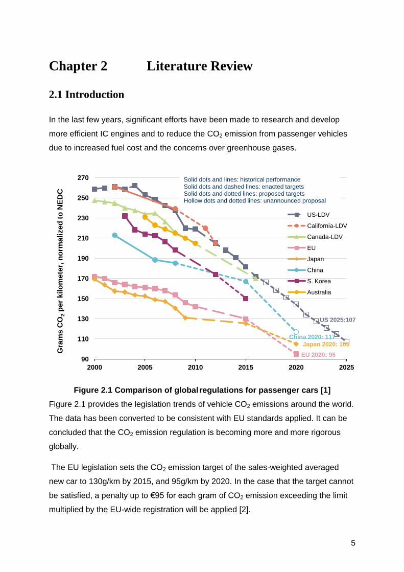
Figure 2.1 Comparison of global regulations for passenger cars [1]
Figure 2.1 provides the legislation trends of vehicle CO2 emissions around the world.
The data has been converted to be consistent with EU standards applied. It can be
concluded that the CO2 emission regulation is becoming more and more rigorous
globally.
The EU legislation sets the CO2 emission target of the sales-weighted averaged
new car to 130g/km by 2015, and 95g/km by 2020. In the case that the target cannot
be satisfied, a penalty up to €95 for each gram of CO2 emission exceeding the limit
multiplied by the EU-wide registration will be applied [2].
US 2025:107
EU 2020: 95
Japan 2020: 105
China 2020: 117
90
110
130
150
170
190
210
230
250
270
2000 2005 2010 2015 2020 2025
Gra
ms
CO
2 p
er
kil
om
ete
r, n
orm
ali
ze
d t
o N
ED
C
US-LDV
California-LDV
Canada-LDV
EU
Japan
China
S. Korea
Australia
Solid dots and lines: historical performance Solid dots and dashed lines: enacted targets Solid dots and dotted lines: proposed targets Hollow dots and dotted lines: unannounced proposal

6
2.2 Advanced engine technologies
In order to improve the engine performance and comply with the legislations, various
technologies have emerged to optimise IC engines.
The fuel delivery system affects the IC engine fuel economy directly. Research
works have indicated that fuel Direct Injection (DI) shows great potential in improving
engine performance. For the conventional engine fuel delivery system, known as
Port Fuel Injection (PFI), fuel is injected onto the back of intake valves via the intake
ports. This method requires the amount of fuel delivered to greatly exceed the ideal
stoichiometric ratio and causes a lag of fuel delivery. This is mainly attributed to the
partial vaporisation of the fuel film on the back of the intake valves. With a direct fuel
injection system, while the fuel is injected directly into the combustion chamber, the
issues of over fuelling with PFI can be reduced and also offers a potential for lean
combustion [3]. The research work of Kume et al. has proved that with fuel direct
injection, especially at part load, the engine can reach very lean combustion, an
air/fuel ratio exceeded 40 could be achieved and significant fuel economy
improvement was found [4]. Also, Toyota [5] has revealed that a stratified in-cylinder
mixture was achieved via Gasoline Direct Injection (GDI) with concaved pistons, and
a 22% fuel consumption reduction was obtained. Another study focused on the in-
cylinder mixture formation and suggested general requirements of combining fuel
direct injection and stratified mixture, such as the air fuel ratio around spark plug
should be 10 to 20, and the spray with 15μm Sauter Mean Diameter (SMD) is
achievable for the in-cylinder swirl flow [6].
The Controlled Auto-Ignition (CAI) combustion, also known as Homogeneous
Charge Compression Ignition (HCCI) is another technique combining the advantages
of both Spark Ignition (SI) and Compression Ignition (CI) methodologies. It is
receiving more and more attention in engine development study and research [7].
CAI/HCCI combustion is achieved by controlling the temperature, pressure, and
composition of the fuel and air mixture, so that it spontaneously ignites the air/fuel
mixture in the engine. This unique characteristic of CAI/HCCI allows the combustion
to occur within very lean or diluted mixtures, resulting in low temperatures that
dramatically reduce engine NOx emissions. Similar to an SI engine the charge is well
mixed which minimises the particulate emissions, also inheriting the advantages of a

7
CI engine being no throttling losses, therefore an overall higher efficiency can be
achieved [8]. Oakley, Zhao and Ladommatos presented an experimental study of
CAI/HCCI combustion in a 4-stroke engine, and the results suggested that with EGR
dilution, the CAI/HCCI improves the fuel economy by 20% at moderate engine load
[9]. In addition, Christens et al. presented that with supercharged CAI/HCCI
favourable 59% net indicated efficiency can be achieved [10].
2.3 Engine downsizing and boosting technologies
Engine downsizing via reducing the total engine capacity is now reasonably
understood as one of the most effective means to reduce the fuel consumption of IC
engines. The idea of engine downsizing concept is to move the engine operation
point towards the higher load region; within such region, the engine normally
performs with higher efficiency. This can be achieved by reducing the engine
displacement, which is known as downsizing, this technique can also be combined
with downspeeding, achieved by adopting higher transmission ratios while used on
vehicle applications. Meanwhile, engine downsizing also reduces the relative
mechanical losses and the engine manufacturing costs.
For example, one research work of Nobuhiro et al. [11] claimed a 12% BSFC
reduction at its maximum torque with a 2.3L boosted gasoline engine delivered
comparative driving performance to 3.0 to 3.5L Natural Aspirated (NA) engine. The
study carried out by Han et al. [12] showed a fuel consumption decrease of 17%
based on Federal Test Procedure (FTP) city mode when replacing a V6 3.3L
gasoline engine with a 2.0L turbocharged Direct Injection Spark Ignition (DISI) unit.
Also, a 0.66L downsized gasoline engine delivered a 5.7% fuel economy
improvement based on the Japanese 10-15 mode [13].
The FORD downsized 1.2L Direct Injection Aluminium Through-Bolt Assembly
(DIATA) diesel engine showed a good compromise between emissions, noise, and
fuel consumption [14]. A downsized 1.5L diesel engine designed by FEV also shows
that by downsizing a 4-cylinder to 3-cylinder benefits the engine performance in
many ways such as fuel economy and et al [15].
Engine downsizing is possible with boosting techniques for the reason of avoiding
the output power and torque penalty due to the reduction of displacement. The

8
boosting systems applied on IC engines normally consist of supercharging and/or
turbocharging. A supercharger usually utilises an air compressor arranged on the
upstream of intake manifold driven by the crankshaft directly. The turbocharger
consists of a turbine, normally propelled by the exhaust gas and a compressor
coupled to the turbine via a common shaft and driven by the turbine. Both systems
have advantages and disadvantages. For supercharger, since the compressor is
driven directly by the crankshaft, response time lag is therefore eliminated, but it
suffers from parasitic losses. Compared to supercharging, turbocharging shows
better performance from its thermodynamic prospective. This is mainly because no
power drained from the engine crankshaft directly to drive the compressor. However
the downside is its poor performance which occurs due to insufficient exhaust gas
energy at low load conditions, where the sufficient power for exhaust gas to drive the
turbine is not yet reached, so the turbocharger cannot operate at its high efficient
region. Furthermore, a response delay which called turbo lag is also associated. This
response delay is mainly due to the acceleration of the rotor of the turbine and the
pressure increase delay because of the flow fluid dynamic characteristic. And at high
engine speed, the turbocharger may elevate the exhaust back pressure, resulting in
pumping losses. This is mainly because of the pressure difference across the turbine,
which created by the turbine itself to drive the compressor.
Turner et al. carried out study on a downsized engine with an ultra-boost system
[16]. The boost system in this case was a combination of a supercharger and a
turbocharger, capable of providing 4.5bar or above to its 5L V8 test engine. The
results suggested that a 23% fuel economy improvement can be achieved with a 60%
downsizing factor. The study of Lake et al. demonstrated another example of
boosted downsized engine [17]. In this work, a substantial fuel economy benefit of
more than 20% has been analysed in comparison with the base NA vehicle whilst
being capable of maintaining half of Euro IV emissions over the NEDC cycle. The
feasibility of replacing larger engines found in compactly sized regular passenger
vehicles with smaller engines has also been investigated by William P. Attard,
Steven Konidaris, Elisa Toulson and Harry C. Watson [18], the study presented that
the performance of a 1.25L NA engine found in the 2007 Ford Fiesta can be
matched by a 0.43L turbocharged engine, meanwhile, the fuel economy
improvement can reach 20%.

9
Although the engine performance can be benefit by downsizing and boosting, there
are numerous limitations of such a technology awaiting advanced solutions to
overcome.
As revealed by the research work of Maria Thirouard and Pierre Pacaud [19], with a
0.5L single cylinder engine, to reach a power density of 80kW/L or above, a boost
pressure of at least 3bar was required, and at 90kW/L the boost pressure level was
found to be 3.4bar, the in-cylinder peak pressure was measured ~200bar.
A research work presented by University of Melbourne revealed the limits of boost
system applications with a supercharger and a turbocharger [20]. The PL was
defined by the author as the Performance Limit, corresponding to the Wide Opening
Throttle (WOT) condition, and the MAP was defined as the Manifold Absolute
Pressure. As shown in Figure 2.2, the engine performance at high speed, high load
area was restricted by the compressor flow limit of the supercharger. Meanwhile, the
high load area suffered from the knocking combustion although it was still below the
failure limit. Turbocharger boosting system in this case was capable of delivering
higher boost pressure. However, at medium speed high load, the engine
performance was limited by the turbocharger flow, and at high speed high load, it
was restricted by the flow limit due to the intake and exhaust system. Meanwhile, the
rest of the high load area can be reached but knocking combustion frequently
occurred. The results also suggested that supercharging are not restricted by the
intake and exhaust system whereas turbocharging suffers from back pressure
elevation.

10
In general, the main technical barriers of downsizing strategy for conventional 4-
stroke engines are as follows [21]:
Combustion limitations – Increased propensity to knock leads to reduced
compression ratio and retarded spark timing, hence lower efficiency
Steady state low speed torque – With increased downsizing, low speed BMEP
requirement increases to maintain acceptable performance
Transient performance – Transient response needs to be maintained with
increased low speed torque requirement
Engine geometry/layout – As engine capacity falls below 1 litre, bore size
and/or cylinder number will require re-optimisation
Part load fuel economy – As downsizing continues the fuel economy gains
inherently reduce due to the limitation of boosting system, measures will need
to be taken to mitigate this
Besides, for gasoline engines, the major technique barriers are also knocking,
thermal and mechanical loads of the engine components, response time of
turbocharging as well as reliability and durability of the engine parts. And for diesel
engines, the main limitation of applying such technology is thermal loads and
consequently the right type of cooling as well as the emission of particulate matter
and nitrogen oxides would become drawbacks within the idea of reducing CO2. And
Supercharged Turbocharged
Figure 2.2 Limits of engine boosted by supercharger and turbocharger [20]
11
to extend the engine working range, the boost system design can be greatly
complicated.
By comparison, the 2-stroke engine has double firing frequency of the 4-stroke, and
for the same output torque its IMEP and the peak pressure are approximately halved.
Thus the 2-stroke engine has much greater potential over the 4-stroke for aggressive
downsizing without having to increase the boost to a degree that 4-stroke engine
demands. These advantages promise to address existing challenges associated with
4-stroke engine downsizing.
2.4 2-stroke engines
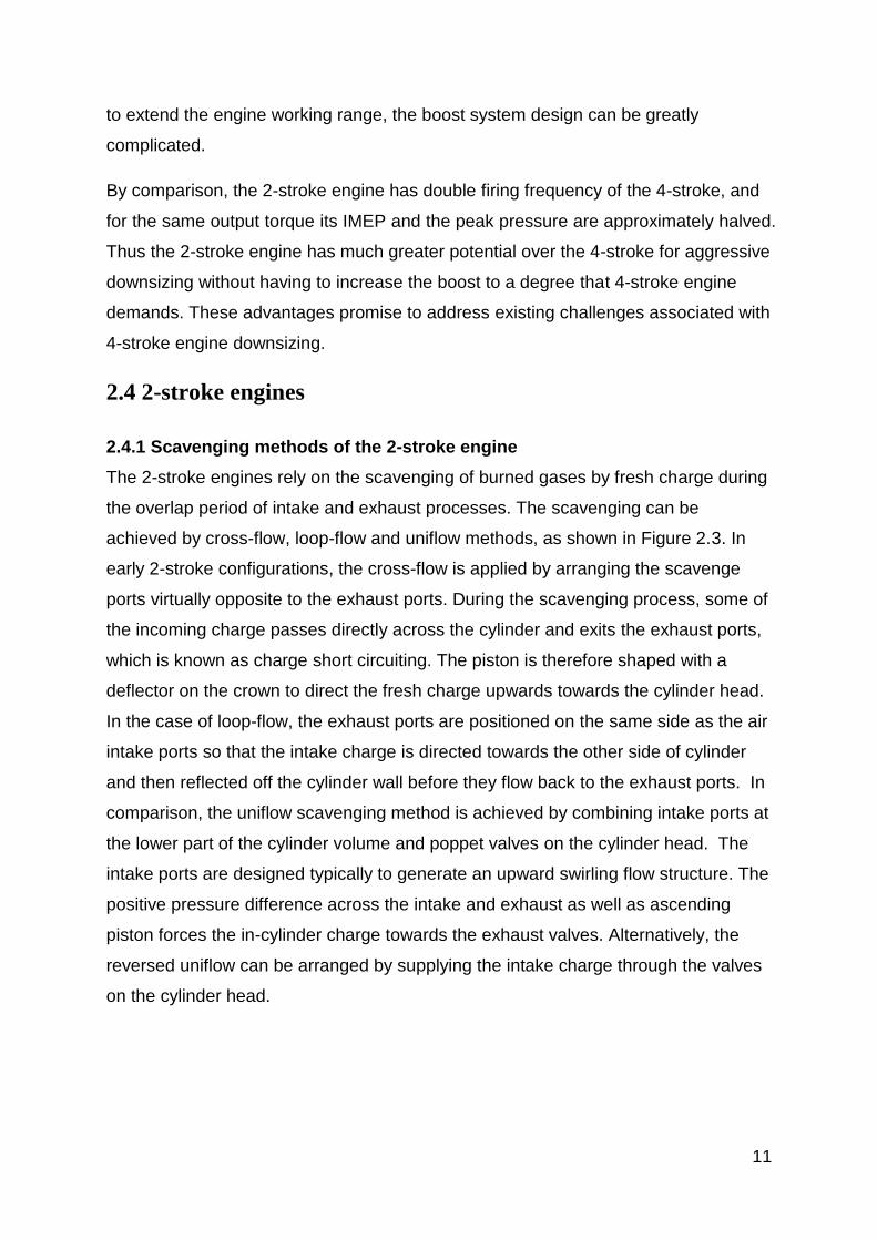
2.4.1 Scavenging methods of the 2-stroke engine
The 2-stroke engines rely on the scavenging of burned gases by fresh charge during
the overlap period of intake and exhaust processes. The scavenging can be
achieved by cross-flow, loop-flow and uniflow methods, as shown in Figure 2.3. In
early 2-stroke configurations, the cross-flow is applied by arranging the scavenge
ports virtually opposite to the exhaust ports. During the scavenging process, some of
the incoming charge passes directly across the cylinder and exits the exhaust ports,
which is known as charge short circuiting. The piston is therefore shaped with a
deflector on the crown to direct the fresh charge upwards towards the cylinder head.
In the case of loop-flow, the exhaust ports are positioned on the same side as the air
intake ports so that the intake charge is directed towards the other side of cylinder
and then reflected off the cylinder wall before they flow back to the exhaust ports. In
comparison, the uniflow scavenging method is achieved by combining intake ports at
the lower part of the cylinder volume and poppet valves on the cylinder head. The
intake ports are designed typically to generate an upward swirling flow structure. The
positive pressure difference across the intake and exhaust as well as ascending
piston forces the in-cylinder charge towards the exhaust valves. Alternatively, the
reversed uniflow can be arranged by supplying the intake charge through the valves
on the cylinder head.

12
Cross-flow Loop-flow Uniflow
Figure 2.3 Typical 2-stroke engine scavenging methods
Among all these scavenging methods, a uniflow 2-stroke engine produces better
scavenging [22] and minimum short circuiting. The short circuiting will deliver fresh
charge directly into exhaust system, wasting the boosted energy, creating a error
measurement of the lambda sensor, and combustion could happen in the exhaust
system. In addition, the uniflow 2-stroke engine can be boosted at higher intake
pressure by closing the exhaust valves earlier and may operate with proven wet
sump and poppet valve technology. The uniflow 2-stroke engine avoids bore
distortion caused by uneven thermal loads in the conventional ported design with its
cold intake port on one side and hot exhaust port on the other. Furthermore, the
uniflow 2-stroke engine is by nature very suitable for CAI combustion operation
which gives stable and fuel efficient part-load operation by adjusting the scavenging
efficiency and hot residual gases through phasing of the poppet exhaust valves
using variable cam timing (VCT) devices. Using CAI addresses the unstable part
load combustion often experienced by the 2-stroke gasoline engine resulting in
further reduced uHC and CO emissions, better fuel economy and significantly lower
NOx emissions. Finally, a centrally mounted injector can be installed in such engines
of smaller bore size due to the absence of intake valves. By combining direct
injection and a uniflow layout, the air and fuel short circuiting associated with
conventional 2-stroke SI engines can be avoided.
13
2.4.2 Previous research on uniflow 2-stroke engines
Uniflow 2-stroke engines are widely used in large marine diesel engines (eg. MAN,
Wärtsilä-Sulzer) and in some diesel locomotives (Electro-Motive Diesel). Detroit
Diesel had been manufacturing uniflow 2-stroke direct injection diesel engines for
heavy duty vehicles until late 1990s as well as for military vehicles requiring very
high power density engines. The most recent and relevant example for passenger
applications is Daihatsu E202 engine shown at the 1999 Frankfurt Motor show [23].
It is a prototype 3-cylinder 987cc, uniflow 2-stroke direct injection diesel engine with
a hybrid scavenging system that combines a supercharger and a turbocharger.
Variable Valve Timing (VVT) was used to control the timing of exhaust valves in the
cylinder head, in order to ensure startability at start-up and best possible fuel
consumption and output. A high pressure common rail fuel injection system was
used to feed centrally located injectors for optimum mixture formation and engine
performance. A 1.0 litre 3-cylinder uniflow 2-stroke direct injection diesel engine
designed for automotive applications was also demonstrated by AVL with a similar
design in the mid 90s [24]. Daimler-Benz conducted an experimental evaluation of a
single cylinder uniflow 2-stroke DI diesel engine and demonstrated that it had similar
performance to the 4-stroke DI diesel engine [25].
However, there have been very few works carried out on the uniflow 2-stroke direct
injection gasoline engine. Chiba University and Fuji Heavy Industry did some
preliminary research on a reverse uniflow 2-stroke direct injection gasoline engine
[26]. In this work, the scavenging processes and in-cylinder flow patterns at various
load and speed conditions were studied using 3D CFD simulation. Universidade do
Minoho presented the design of a single cylinder crankcase boosted semi-direct
injection gasoline uniflow 2-stroke engine of 43.3cm3 displacement volume [27]. The
engine was predicted to produce a rated BMEP of 8bar and was intended for a
student marathon fuel economy competition.
As discussed above, for 2-stroke engines, the scavenging process plays significant
role to the engine performance. And among all scavenging methods, the uniflow
shows best scavenging efficiency. Daimler-Benz AG presented a study of 2-stroke
engines with common rail fuel supply systems [25]. The study compared the
performance of 2-stroke loop-flow and uniflow configurations. As shown in Figure 2.4,

14
the uniflow method shows better performance than the loop-flow under similar
engine conditions.
Figure 2.4 Full-load performance of loop-flow and uniflow 2-stroke engine [25]
Although the uniflow scavenging shows superior performance, the uniflow
scavenging method has a disadvantage. It is the significantly greater cylinder
spacing and the unfavourable overall engine lengths. When the engine bore/stroke
ratio is extremely high of low, it is very hard for the intake port design to optimize and
generate a proper flow to blow the residual gas due to the spatial narrow shape. AVL
carried out research work on the intake port to optimise the scavenging process of
the uniflow 2-stroke engine [24]. As shown in Figure 2.5, a), the conventional intake
port arrangement and b) illustrated the optimised intake port arrangement. With
careful design of the size and orientation of the intake ports, the lack of scavenging
ability around the centre of the engine can be overcome.

15
a)
b)
Figure 2.5 In-cylinder flow structure (a) (b) [24]
Being different from the conventional 4-stroke engine, the boost system for 2-stroke
engines is indispensable. It is due to the scavenging method for 2-stroke engine

16
breathing, that the intake and exhaust processes have much greater overlap than 4-
stroke engines. The boost system of a 2-stroke engine requires careful optimisation.
Mattarelli et al. published their study on a 2-stroke GDI engine [28]. The study
revealed the strategy of boost system optimisation on 2-stroke engines. For a
supercharger, it is relatively easy to increase the engine power & torque,
unfortunately, the fuel consumption also increases due to the mechanical losses.
The strategy is to keep the boost pressure as low as possible while the engine power
target is satisfied. For a turbocharger, the conflict is that while the requirement of
boost pressure is higher, the turbine nozzle size has to be smaller. However, the
exhaust pressure will increase and therefore the fuel consumption increases too.
The strategy of turbocharger optimisation is to compromise the nozzle size and the
required boost pressure.
2.5 In-cylinder flow measurements
The in-cylinder flow structure has a great effect on the engine gas-exchange, air/fuel
mixing, combustion and output performance [22]. For conventional engines, large
scale flow structures, such as swirl or tumble are often used to maintain the flow's
kinetic energy until the end of the compression stroke, where they break down into
micro scale turbulence, promoting early flame kernel growth and increased flame
speed [29], which increases the engines knock limit, allowing the use of increased
compression ratios that result in increase fuel efficiency and reduced CO2 emissions.
In addition, higher flame speed allows leaner air/fuel mixture to be burned for better
fuel economy. For uniflow 2-stroke engine, the effect of in-cylinder flow organisation
is even more significant on the engine performance. In order to provide information
to optimise the in-cylinder flow structure, the in-cylinder flow investigation is required.
Despite the development of ever more powerful CFD modelling tools that are of
great value to designers of such combustion systems, their limitations mean that
experimental validation of models will still be required for the foreseeable future.
The Hot Wire Anemometry (HWA) and Laser Doppler Anemometry/Velocimetry
(LDA/LDV) methods have been developed to provide single point flow data [30]
[31][32][33][34][35]. The complex flow structure in the cylinder is better measured by
the spatially resolved flow field measurement techniques. In early stage of the in-
cylinder flow structure studies, smoke, metaldehyde crystals and white goose down

17
cut into short pieces after the heavier pieces had been removed were all used as the
mediums to trace the in-cylinder air flow [36]. The quantitative whole field
measurement began with the development of Particle Tracking Velocimetry (PTV)
[37][38][39] and Particle Image Velocimetry (PIV) [40][41][42]. Such techniques have
been developed and enabled to provide instantaneous, cycle resolved, two-
dimensional velocity maps across extended measurement planes within the cylinder.
With these in-cylinder flow measurement methods, small seeding particles are
required to indicate the flow movement, the seeding particles are normally planted at
the upstream of the intake ports, and then illuminated by a certain light source, such
as lasers in most of the cases, so two frames recorded within a very short time
interval can be obtained.
With the PTV technique, the particles are identified individually and correlated
between two exposures taken in a narrow time window, the particles velocity vectors
can be determined by their displacements. The PTV method has been used to
conduct an extensive in-cylinder flow visualisation study. For example, the research
of the intake-generated fluid motion produced different intake configurations [43], the
cyclic variability of the pre-combustion flow field in a motored engine [44], and the
effects of intake port configurations on in-cylinder flow organisation [45]. These
previous research works have proved that the PTV method is able to provide useful
data for in-cylinder flow study. However, there are several technique barriers that
restrict the application within engine research. Firstly, the light source for the PTV
method is required to be with long pulses, this requirement leads to a low power
density of the illumination of seeding particles. To provide images with adequate
quality, the seeding particles have to be large size so they can scatter sufficient light
to be captured by cameras. Furthermore, because of the combination of low light
power density and large size seeding particles, the planting density of the particles
has to be low in order to avoid confusion of seed pairs during analysis, the lean flow
will increase the load of post-processing works.
The development of the PIV technique and its application to IC engines has allowed
in-cylinder flow field measurement to be obtained with high spatial resolution. For
PIV measurements, the seeding particles are illuminated by high energy, thin laser
sheet pulses, and two frames are captured in a very short duration. The whole region
of interest is divided into small interrogation areas, the mean flow velocity vectors are

18
calculated within these interrogation areas, typically with a cross-correlation method.
By doing so, the identification of distinct, individual particles is no longer required.
The illumination light source for PIV with short pulse and high power density allows
the use of micron sized particles that can track high frequency flows. The high
density seeding particles is allowed to be used, so a more comprehensive velocity
map can be obtained than with PTV. The PIV method is suitable for the
measurement of both large scale and small scale flow structures.
General Motors R&D Centre has carried out a study applying PIV technique to take
measurements of in-cylinder flow velocity in order to calculate the swirl and tumble.
The results were also compared with numerical calculation results [46]. The
experiments were carried out on a motored 4-stroke engine, and the measured and
computed turbulence distributions at TDC compression both show a maximum near
the cylinder centre that agreed to within 25% of each other. Apart from running PIV
on combustion investigation, David L. Reuss has also carried out a study using PIV
technique to a motored engine [47], this study proved that not only a steady in-
cylinder flow structure can be created, but also a flow structure with different scale
can be achieved within the same cycle. The research of Haider et al. applied the PIV
technique to a large 2-stroke marine engine [48], the study focused on the effect of
the piston position to the in-cylinder flow structure while the intake ports were
partially and fully opened.
2.6 In-cylinder fuel distribution
The effort of the engine in-cylinder fuel distribution and the air/fuel mixing process
affects the engine performance to a great extend. In the case of a 2-stroke direct
injection engine, the fuel atomisation and mixture formation are even more important
due to the reduced time for the mixing process.
Several non-intrusive laser based diagnostic techniques have been developed to
allow in-cylinder fuel concentration measurement. The major techniques are based
on Rayleigh scattering, Raman scattering and laser induced fluorescence.
The Laser Rayleigh Scattering (LRS) is a simple and user friendly method for
measuring gaseous species concentration. The Rayleigh scattering signal is the
strongest among the three techniques mentioned above. However, the LRS method

19
suffers from the interference of the Rayleigh signal by Mie scattered light from both
solid and liquid particles and the cylinder walls and it is not species specific. LRS
was used in some early studies of in-cylinder fuel vapour distribution. For example,
the concentration of Freon-12 vapour from diesel injector was measured by LRS to
study the simulated diesel injection process in [49]. The in-cylinder gasoline fuel
vapour concentration in a motored engine was measured by LRS through careful
optical arrangement and calibration. A research work focused on a steady flow rig
was presented in a series of studies [50]. A more substantial case of LRS application
was presented for the fuel vapour concentration measurement in an evaporating and
combusting spray in an optical DI diesel engine under fired and motored conditions
[51].
The Spontaneous Raman Scattering (SRS) technique is capable of providing
simultaneous multiple-species measurements of major species such as N2, O2 and
CO2 and etc. With the appropriate laser and multi-channel detector developed, multi-
point, multi-species SRS measurements have been demonstrated [52]. But the SRS
suffers from very weak signal-to-noise ratio due to the small Raman scattering cross
section.
Among all three techniques, the Laser-Induced Fluorescence (LIF) is probably the
most successful and the most widely used for engine fuel distribution studies. The
main reason of its success is the ability of providing fuel distribution data with a good
signal to noise ratio. With proper calibration, this method can be used to obtain
quantitative air/fuel ratio measurements.
According to the work of Christof Schulz and Volker Sick [53], the ideal tracer for LIF
should behave like the base fuel used, and should yield LIF signal intensities that are
directly proportional to the desired quantity and should not be influenced by the
ambient conditions. Toluene has been used as LIF tracer in research work carried
out by Sandia National Laboratories [54], while an Nd:YAG laser (266 nm) was used
as the excitation source, and iso-octane was used as the fuel because of their similar
boiling points. The inert gas in this case was N2, because the tracer toluene
experienced fluorescence quenching problems due to oxygen. Another research
applied PLIF technique to a DISI engine using same laser light source, the tracer in
this study was 3-pentanone, and to compensate the early depletion of the 3-

20
pentanone, 3- hexanone was also used. The advantages of 3-pentanone for fuel
distribution measurements is that its boiling point (102ºC) closely matches the iso-
octane (99ºC) at ambient temperature and pressure. However, evidences also
indicated that Rapid depletion of 3-pentanone in the liquid mixture shows significant
uncertainties in iso-octane distribution measurements, especially in a GDI engine
when the fuel is evaporated in the combustion chamber [55]. A very recent
publication of LIF technique applied on a GDI engine was carried out by Changan
Automobile Company [56]. In this research work, a KrF excimer laser with the
wavelength of 248nm is used as the excited laser source. The tracer was 3-
pentanone and it was mixed up with iso-octane with a 1:9 ratio in volume. The
properties of iso-octane and 3-pentanone are shown in Table 2.1.
Table 2.1 Key properties of the experimental fuels and dopant
Iso-Octane 3-Pentanone
Lower Heating Value
(MJ/kg) 44.31 33.4
RON 100 -
MON 100 -
(R+M)/2 100 -
Density at 15ºC (kg/dm3) 0.69 0.81
H/C Ratio 2.25 2
O2 (% weight) 0 18.6
2.7 Summary
This chapter presents the related research literature dedicated to reducing the
engine fuel consumption, and also many related techniques applied to IC engines.
Studies suggest that engine downsizing is a very effective way to reduce the engine
CO2 emission. However, some technical barriers restrict the further downsizing of 4-
stroke gasoline engines, such as knocking, thermal and mechanical loads of the
engine components, response time of turbocharging as well as reliability and
durability of the engine.
21
On the other hand, the 2-stroke engine has double firing frequency of the 4-stroke,
Thus the 2-stroke engine has much greater potential over the 4-stroke for aggressive
downsizing without having to increase the boost to a degree that 4-stroke engine
demands.
One big issue of 2-stroke engine optimisation is the scavenging process. Several
scavenging methods are available for 2-stroke operation, such as cross-flow, loop-
flow and uniflow. In comparison, uniflow has the best scavenging performance. By
combining uniflow and direct injection in a 2-stroke operation, the fuel consumption
can be improved through aggressive engine downsizing with the absence of typical
ported 2-stroke engines.
Optical diagnostic techniques are very helpful for providing engine in-cylinder
information. Various types of optical diagnostic and their applications on IC engine
studies have been discussed. The PIV technique is identified as the most suitable
technique for the in-cylinder flow measurements of the uniflow 2-stroke engine. The
PLIF technique is selected for the in-cylinder fuel distribution due to its suitability,
strong signal and relatively simple setup.
22
Chapter 3 Analytical studies of flow and mixing in
a uniflow 2-stroke engine
3.1 Introduction
Over the past decade, the numerical analysis has been extensively used for
engineering design and optimisation. In the research and development of the IC
engine, the Computational Fluid Dynamics (CFD) is increasingly used for the
analysis of in-cylinder flow, mixture formation and combustion.
In the current study, the CFD method was used to investigate the in-cylinder flow
pattern, the fuel injection process and the air/fuel mixing process in the direct
injection gasoline uniflow 2-stroke engine. The results were also used to provide the
initial and boundary conditions in the 1-D engine simulation for optimising the intake
ports, the exhaust valve timing, and the prediction of the engine’s performance.
As the computational hardware and techniques develop, the numerical analysis on
IC engines play a more and more important role to research and hardware
optimisation. The traditional methods of engine research and development is
following the procedure as:
Building prototype engines
Running tests on the test bed to gain relevant information
Modifying the prototype according to the test results to optimise the engine
The traditional way of engine research is a costly and highly time consuming process
due to the large number of variables that have an effect on the design. Numerical
engine study and analysis plays a very important role in the development of engines.
It helps in analyzing the various engine configurations without actually building the
engine. Thus, Engine Simulation helps in reducing the cost and time involved in
developing a new engine [57].
The state-of-the-art of computational simulation has advanced on many fronts.
Nowadays, computer hardware itself has improved dramatically over the last half
century. As we close the 20th century, computers are 109 times faster and more cost

23
effective than they were in the days of World War II. The computational expense
reduces by a factor 2 every 1.5–2 years, which fits well with this remarkable
performance achievement. Furthermore, while state-of-the-art electronic chip
manufacturing today uses 0.25μm feature size technology, the path to 0.05μm or
smaller technology now seems apparent, thereby ensuring same speedup rate for
the next 15 years or so [58]. The development of computational technology secures
the numerical analysis method plays a role as important and experimental studies on
IC engines.
3.1.1 Introduction to CFD simulation
CFD is the abbreviation of Computational Fluid Dynamics. It is computational
method that uses numerical methods and algorithms to solve and analyze problems
that involve fluid flows. Numerical simulations of CFD are normally used for two
purposes. First, the applications of CFD are associated with fundamental research.
This kind of studies requires very high accuracy of the numerical data; the physical
models used to present the fluid behaviour must be pertinent and so are the
algorithms used. Second, the CFD simulation is used to predict the flow
characteristic. The goal here is to predict physical characteristic of the flow structure
and its efforts on certain objects rather than providing data for flow dynamics itself. In
this case, the introduction of CFD simulation is on purpose of reducing the cost and
time required to develop a study subject [59]. This technique has been widely used
for the studies of flow structure, fuel spray and distribution and combustion
organisation on IC engines. The applications of CFD simulation on engine research
is used mostly for the second purposed. Many commercial types of software have
been developed for the purpose of CFD simulation, the software used for the study
related to the work described in this article is the Ansys Fluent.
3.1.2 Turbulence model
It is an unfortunate fact that no single turbulence model is universally accepted as
being superior for all classes of problems. The choice of turbulence model will
depend on considerations such as the physics encompassed in the flow, the
established practice for a specific class of problem, the level of accuracy required,
the available computational resources, and the amount of time available for the
simulation.

24
For the turbulent simulation, also there are many models can be used to calculate
the flow structure. The Reynolds-averaged Navier-Stokes (RANS) and Large-eddy
simulation (LES) are two most popular modelling methods of IC engine applications.
Both methods use similar equations and are based on same principle ground.
However, in terms of physical meanings of parameters in the equations, the
difference is identified.
3.1.2.1 Reynolds-Averaged Approach
Time-dependent solutions of the Navier-Stokes equations for high Reynolds-number
turbulent flows in complex geometries which set out to resolve all the way down to
the smallest scales of the motions are unlikely to be attainable for some time to
come. One of the methods can be employed to render the Navier-Stokes equations
tractable so that the small-scale turbulent fluctuations do not have to be directly
simulated. It is the Reynolds-averaging approach.
The Reynolds-Averaged Navier-Stokes (RANS) equations govern the transport of
the averaged flow quantities, with the whole range of the scales of turbulence being
modeled. The RANS-based modelling approach therefore greatly reduces the
required computational effort and resources, and is widely adopted for practical
engineering applications.
The flow of a viscous incompressible fluid with constant properties is governed by
the Navier–Stokes equations (Einstein summation convention applies to repeated
indices) [60].
[E-3.1]
[E-3.2]
– The fluid velocity
– The pressure
– The fluid kinematic viscosity
The dependent variables of Equation 3.1 and 3.2 can be decomposed into mean and
fluctuating parts as follow,

25
[E-3.3]
By substituting Equation 3.3 into Equation 3.1 and 3.2, taking an ensemble average,
the system of partial differential equations that governs the mean-velocity and
pressure fields of incompressible turbulent flow can be derived as follows,
[E-3.4]
[E-3.5]
With reference to the nonlinear term shown below,
[E-3.6]
The RANS can be derived as follow,
[E-3.7]
[E-3.8]
– The Reynolds-stress term that incorporates the effects of turbulent motions
on the mean stresses
3.1.2.2 Large-Eddy Simulation
LES provides an alternative approach in which large eddies are explicitly computed
in a time-dependent simulation using the filtered Navier-Stokes equations. The
rationale behind LES is that by modelling less of turbulence, the error introduced by
turbulence modelling can be reduced. It is also believed to be easier to find a
universal model for the small scales, since they tend to be more isotropic and less
affected by the macroscopic features like boundary conditions, than the large eddies.
Filtering is essentially a mathematical manipulation of the exact Navier-Stokes
equations to remove eddies that are smaller than the size of the filter, which is
usually taken as the mesh size when spatial filtering is employed. Like Reynolds-
averaging, the filtering process creates additional unknown terms that must be
modeled to achieve closure. Statistics of the time-varying flow-fields such as time-
averages values of the solution variables, which are generally of most engineering
interest, can be collected during the time-dependent simulation. LES for high

26
Reynolds number industrial flows requires a significant amount of computational
resources. This is mainly because of the need to accurately resolve the energy
containing turbulent eddies in both space and time domains, which becomes most
acute in near-wall regions where the scales to be resolved become much smaller.
Wall functions in combination with a coarse near wall mesh can be employed, often
with some success, to reduce the cost of LES for wall-bounded flows. However, one
needs to carefully consider the ramification of using wall functions for the flow in
question. For the same reason (to accurately resolve eddies), LES also requires
highly accurate spatial and temporal discretizations.
In general, the LES model shows advantages in details of flow structure, such as
eddies and vortices. Furthermore, LES model has the potential to be more predictive.
However, the assumption of potential of prediction is based on the solver calculation
methods, but this assumption is hard to be validated, and the settings of boundary
conditions will contribute to the result variations of LES to further extend than RANS.
In contrast, the RANS shows advantages in resulting a time based average data,
which is more compatible with experimental results, and the computational time
expense is lower than LES with same grid conditions.
Research Institute of Automotive Engineering and Vehicle Engines Stuttgart has
carried out 3D CFD simulations in order to provide information for the intake system
design on an 8-cylinder engine with external exhaust gas recirculation [61]. CFD
simulation also has been used to investigate the evaluation of the effects of cycle by
cycle variation on knock tendency of a high performance spark ignition engine [62],
the simulation data provided qualitative information for the identification of best park
plug location. The study of Cornolti et al [63] presents different methodologies of
CFD analysis applied to the intake plenum of a turbocharged HSDI Diesel engine.
The discharge and pressure loss coefficients representing the flow losses within the
plenum have been calculated. The comparison with the steady flow bench
experimental results confirmed the accuracy of the 3D model.
3.2 CFD Model Set-Up
ANSYS FLUENT was chosen for the simulation. Fluent has a powerful pre-processor
to import geometry files from CAD and provides high quality mesh creating ability
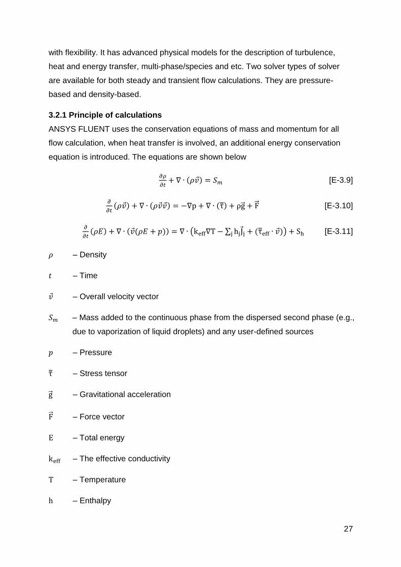
27
with flexibility. It has advanced physical models for the description of turbulence,
heat and energy transfer, multi-phase/species and etc. Two solver types of solver
are available for both steady and transient flow calculations. They are pressure-
based and density-based.
3.2.1 Principle of calculations
ANSYS FLUENT uses the conservation equations of mass and momentum for all
flow calculation, when heat transfer is involved, an additional energy conservation
equation is introduced. The equations are shown below
[E-3.9]
[E-3.10]
[E-3.11]
– Density
– Time
– Overall velocity vector
– Mass added to the continuous phase from the dispersed second phase (e.g.,
due to vaporization of liquid droplets) and any user-defined sources
– Pressure
– Stress tensor
– Gravitational acceleration
– Force vector
– Total energy
– The effective conductivity
– Temperature
– Enthalpy

28
– The diffusion flux of species j
– The heat of chemical reaction, and any other volumetric heat sources
defined by user
Equation 3.9 and Equation 3.10 describe the conservation of mass and momentum
respectively. The equation of energy conservation shows as Equation 3.11 [64].
One of the main targets for the study is to investigate and predict the in-cylinder
turbulent flows and the swirl generating ability with corresponding intake port designs.
There are different fluid flow-modelling techniques.
The RANS calculation method was applied for the flow structure simulation in this
study and the turbulence model used was Re-Normalisation Group (RNG)
model. The RNG model is derived using a rigorous statistical technique with
following features:
The RNG model has an additional term in its equation that significantly
improves the accuracy for rapidly strained flows.
The effect of swirl on turbulence is included in the RNG model, enhancing
accuracy for swirling flows.
The RNG theory provides an analytical formula for turbulent Prandtl numbers,
while the standard model uses user-specified, constant values.
While the standard model is a high-Reynolds-number model, the RNG theory
provides an analytically-derived differential formula for effective viscosity that
accounts for low-Reynolds-number effects. Effective use of this feature does,
however, depend on an appropriate treatment of the near-wall region.
These features make the RNG model more accurate and reliable for a wider
class of flows than the standard model [64].
Transport Equations for the RNG Model are shown below:
[E-3.12]
[E-3.13]

29
– Turbulence kinetic energy
– Turbulence dissipation rate
– Generation of turbulence kinetic energy due to the mean velocity gradients
– Generation of turbulence kinetic energy due to buoyancy
– Contribution of the fluctuating dilatation in compressible turbulence to the
overall dissipation rate
– Constants
– Inverse effective Prandtl numbers for and , respectively
– User-define boundary
By solving equation set combined by equation 3.12 and 3.13, the value of and
can be derived.
3.2.2 Boundary Conditions
To define the calculation, the boundary conditions are as important as the physical
equations. The boundary conditions include mechanical structure codes, engine
breathing inlet/outlet pressure and temperature, piston movement profile, valve lift
profiles and etc.
For the mechanical structure, the basic engine parameters are the bore and stroke,
the intake port geometry configuration, exhaust valves dimensions and etc. The
engine mechanical structure is defined by Pro Engineering, and then imported into
the CFD tools. All engine mechanical structures were defined prior to the CFD
calculations.
The other boundary conditions can be generated after the mechanical code is
imported into CFD tools and meshed. For the engine modelling system, in terms of
mass flow transfer, inlet/outlet boundary conditions are required to describe the
intake/exhaust conditions on the interface between the engine model and the global
environment, including:
Pressure on the environment side of the inlet/outlet interface.

30
Flow direction on the inlet/outlet interface.
Turbulent kinetic energy and dissipation rate.
Temperature of the flow at the boundary interface.
The components of the inlet species and exhaust species if backflow occurs
at the exhaust outlet boundary
The dynamic mesh boundaries for the engine structure are piston and exhaust
valves. The piston movement is defined by the engine geometry configurations,
including:
Crank shaft speed
Piston stroke
Connecting rod length
In FLUENT, the piston location is calculated by
[E-3.14]
– Piston location from TDC at specified crank angle
– Length of connecting rod
– Engine stroke
– Crank angle
The exhaust valve lift profile is defined by a code contains the crank angle and
corresponding valve lift, which is created separately and then imported into the CFD
tool. During the simulation, the valve moving axis is defined and the valve position at
a given crank angle is then governed by the valve lift profile.
3.2.3 Grid and Mesh Types
CFD calculations are based on the finite element method by discretizing the
geometry into grids. By doing this, the formula to solve the problem related to the
geometry is also discretized and integrated into a matrix which describes the
physical problems.

31
The grids will have great impact on the convergence rate of calculation, the accuracy
of the calculation and the calculation time consumption.
The typical grid types of 2D and 3D are shown in Figure 3.1.

32
Triangle Quadrilateral
2D Grid Types
Tetrahedron Hexahedron
Wedge Pyramid
3D Grid Types
Figure 3.1 Typical Grid Shapes
The grid details of the CFD calculation in this study will be discussed in following
chapters.

33
3.3 CFD Calculation with 2D Model
The performance of the uniflow 2-stroke engine is largely determined by the
scavenging process during the overlap period of intake and exhaust opening. In a
uniflow 2-stroke engine, intake ports geometry and opening time determine the
intake fresh charge mass flow rate, the scavenging performance, and the swirl
generation of in-cylinder flow.
At the start of the project, a single cylinder 2-dimensional uniflow 2-stroke engine
base model was set up for the study of scavenging process and the optimisation of
the intake ports. The engine model features intake ports at the bottom of the cylinder
liner. Exhaust valves are included in the cylinder head and actuated by a camshaft.
A set of parameters are introduced [22] to define the intake port configuration
settings of the uniflow 2-stroke engine, as shown in Figure 3.2 and Table 3.1.
(a) (b)
Figure 3.2 The intake port geometry parameter

34
Table 3.1 The intake port geometry parameter
Parameter Definition
rcy engine bore
rp radius of swirl circle
θp port width angle
N Number of ports
Ai Axis inclination angle
φp Swirl orientation angle
xp Effective port width
θb Port shoulder width angle
xb Effective port shoulder width
3.3.1 2D Model Design
In order to determine a baseline configuration of the uniflow 2-stroke engine, a 2D
CFD model was first used to predict the effect of axis inclination angle, Ai, on in-
cylinder flow and the scavenging process during the overlap period of intake port
opening and exhaust valve opening. The 2D model is shown in Figure 3.3.

35
Figure 3.3 The 2D CFD model
At this stage, the engine bore is set to 80mm and stroke is set to 89mm, which will
be used for the single cylinder engine experiments later.
As shown in Figure 3.3, the engine geometry structure has been simplified and
divided into 5 groups, which are shown below,
A1 and A2 – Exhaust valves
B1 and B2 – Valve dynamic zones
C – Clearance volume
D – Swept Volume
E1 and E2 – Intake port channels
The reason of simplification and the divisions of the geometry structure is that two
moving groups were involved, exhaust valves and piston. So the dynamic mesh has
to be assigned. To secure the transient calculation process, a structured grid is
chosen. In this case, the quadrilateral grid type is chosen. The structured grid
requires less time and achieves best transient calculation performance when
dynamic mesh is applied. In addition, the performance of mesh regeneration and
calculation convergence performance are better.

36
Figure 3.4 Boundary of exhaust valves
Figure 3.4 shows the mesh structure and boundary setup of the exhaust valves. The
top edge of exhaust valve meshes is set to be an outlet boundary which is the outlet
of the entire system. The back-pressure is set to the ambient pressure. The backflow
component can be also defined and are set to be burnt gas. The side walls of the
exhaust valves meshes are set to as interfaces. The interface allows mass and
energy transfer across and is mainly used with dynamic mesh and moving
components. Because of the valves movement, the interface here is set to couple
with the corresponding interface on the valve dynamic zones. When the valves
move down, the couple of interface sets overlaps and the in-cylinder components
and the energy are allowed to travel from one side to the other freely. As a result,
when the exhaust valves are opened, the in-cylinder components are allowed to
follow the flow towards the outlet boundary. All other edges are set to solid walls
including those in the interior. The entire valve zone moves as a rigid body so the
mesh and boundary edges posses exactly the same relative positions during the
simulation. The valve movement is controlled by a user defined lift profile.

37
Figure 3.5 Boundary of valve dynamic zones and clearance volume zone
The clearance volume zone and valve dynamic zones are shown in Figure 3.5. The
grid type for these two zones is also structured quadrilateral. The clearance volume
zone has two sets of interfaces and the other edges are walls. Two interface sets are
coupled with the swept volume and the valve dynamic zones respectively, both
allows the in-cylinder components to travel freely in the cylinder chamber.
The top edge of valve dynamic zone adjacent to the exhaust valve is set to wall and
the other edges are set to interface. When the exhaust valve is moving, the vertical
length of valve dynamic zone changes. The interior mesh is squeezed when valves
move down and expanded when valves move up. The quadrilateral grid is applied to
the valve dynamic zone. When valves move during the simulation, the layers of
mesh are recalculated and regenerated. The layers adjacent the moving side are
removed when mesh is squeezed and added when mesh expands. The grids on the
rest of zones remain the same. Different types of grid of mesh has been applied to
the model, a set of preliminary simulation has been carried out under same boundary
conditions. The results suggested this meshing method gives the best convergence
ability and requires less computing time.

38
Figure 3.6 Boundary of swept volume
The swept volume zone is shown in Figure 3.6. The dynamic mesh design is the
same as the valve dynamic zone. The bottom edge of the swept volume zone is set
to be the piston. The movement is defined by the pre-defined engine speed, piston
stroke and connecting rod length. The interior mesh is also regenerated by removing
and adding layers. Two sets of interfaces are defined, one set couples with the
corresponding interface on clearance volume, the other couples with the intake port
channels.
Figure 3.7 Boundary of intake port channel

39
As shown in Figure 3.7, the far side of the intake port channel is set to the inlet
boundary. The inlet pressure, temperature, species and initial flow direction is
defined and assigned to the inlet boundary. On the edge adjacent to the swept
volume zone, the edge is defined as interface coupling with the swept volume zone.
3.3.2 2D Model simulation and results
The intake ports opening time is governed by their relative location to the piston at
BDC. When the piston position is higher than the port top edge, the ports are fully
covered by the piston, and the intake ports are closed. When the piston location is
lower than the top edge of intake ports, the intake ports are opened. The exhaust
valves timing is governed by their lift profile.
The calculation started from 120°ATDC, at which exhaust valves start to open, to
250°ATDC, when the intake ports are fully covered by the piston and the exhaust
valves are closed. Thus, simulation covers the range from the beginning to the end
of the scavenging process of the 2-stroke operation.
A 1.5bar absolute boost pressure was applied to the intake flow. The initial in-
cylinder pressure was set to 1.2bar @120°ATDC, and in-cylinder temperature was
set to 500K. The initial in-cylinder charge was assumed to be stationary. The
exhaust backpressure was set at the ambient pressure.
The following parameters are used to characterise the quality of scavenging process
[66]:
Delivery Ratio (DR): defined as the ratio of delivered fresh charge mass to
reference mass. The reference mass is calculated by the displaced volume
multiplied by ambient air density.
Trapping Efficiency (TE): defined as the ratio of mass of delivered fresh
charge retained in the in-cylinder to the total mass of delivered fresh charge.
Scavenging Efficiency (SE): defined as the ratio of mass of delivered fresh
charge retained in the cylinder to the total trapped cylinder charge.
Charging Efficiency (CE): defined as the ratio of mass of delivered air retained
in the cylinder to the reference mass.
Calculations were carried out for 5 intake port’s axis inclination angles, Ai,
which are 30º, 45 º, 60 º, 90 º and 135 º as shown in Figure 3.8.
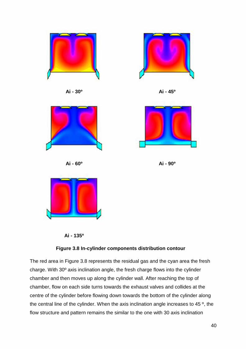
40
Ai - 30º Ai - 45º
Ai - 60º Ai - 90º
Ai - 135º
Figure 3.8 In-cylinder components distribution contour
The red area in Figure 3.8 represents the residual gas and the cyan area the fresh
charge. With 30º axis inclination angle, the fresh charge flows into the cylinder
chamber and then moves up along the cylinder wall. After reaching the top of
chamber, flow on each side turns towards the exhaust valves and collides at the
centre of the cylinder before flowing down towards the bottom of the cylinder along
the central line of the cylinder. When the axis inclination angle increases to 45 º, the
flow structure and pattern remains the similar to the one with 30 axis inclination

41
angle intake ports. However, the fresh charge occupies more area and flows further
down at central line of the cylinder in a reversed vortex shape. With 60 º axis
inclination angle, the flow structure of fresh charge is distributed in an area of the
shape of an upside-down wine cup. The sides of fresh charge area are formed at the
same angle as intake ports and converge towards each other before diverging
upwards to the exhaust valves. With 90 º and 135 º intake port inclination angle, the
fresh charge moves along the piston top and collides to form a vertical flow along the
central line towards the top of the cylinder chamber.
The cumulative results of delivery ratio, charging efficiency, scavenging efficiency
and trapping efficiency over the scavenging period are shown in Figure 3.9.
Figure 3.9 Engine scavenging performance as a function of axis inclination
angle based on 2D models
The delivery ratio reaches its peak at 90º intake port inclination angle. Either
increase or decrease in the axis inclination angle will cause a drop of the delivery
ratio. This is better explained by the effective area ratio of intake port, which is
defined as
400%
420%
440%
460%
480%
500%
520%
540%
560%
30° 45° 60° 90° 135°
Delivery Ratio
10%
10%
11%
11%
12%
12%
13%
30° 45° 60° 90° 135°
Trapping Efficiency
50%
52%
54%
56%
58%
60%
62%
30° 45° 60° 90° 135°
Charging Efficiency
88%
90%
92%
94%
96%
98%
100%
30° 45° 60° 90° 135°
Scavenging Efficiency

42
[E-3.15]
– Effective ratio of area
– Effective area of intake port
– Intake port area along the cylinder wall
– Axis inclination angle
And the definition of , , and is shown in Figure 3.10.
When the intake port inclination angle is 90º, the effective area ratio of intake port
reaches 1.
Figure 3.10 Effective area ratio of intake port
But 90º axis inclination angle intake ports resulted in the lowest trapping efficiency,
because of the “short-circuiting” phenomenon [22], which involves the fresh charge
going directly out of the cylinder through the exhaust valves during the scavenging
period. As shown in Figure 3.8, with 90º axis inclination angle intake port, some of
the fresh charge can flow to the exhaust valves and escape the cylinder chamber.
The 30º axis inclination angle intake port has the highest trapping efficiency but the
lowest delivery ratio.
The charging efficiency, indicating the charging ability of the intake system, reaches
its maximum value with 60º axis inclination angle intake port. The scavenging

43
efficiency shows the same trend as the charging efficiency and indicates the ability of
fresh charge blowing the residual gas out of the cylinder chamber. Because the
charging efficiency has most direct impact on the engine power output, the 2D
calculation suggests that the 60 º axis inclination angle intake ports can be adopted
for maximum engine output.
3.4 3D CFD Calculations
3.4.1 3D CFD engine model
In order to carry on more realistic simulations, a 3D engine CFD model is set up as
shown in Figure 3.11. The base engine is based on the engine geometry of the
single cylinder engine to be used for experimental studies and it has an 80mm bore
and 89mm stroke. The cylinder head includes a pent roof combustion chamber and
four valves.
Figure 3.11 3-D CFD base model
Similar to the 2D model, the entire engine geometry is divided into 5 groups, exhaust
valves, valve dynamic zones, clearance volume, swept volume and intake port
channel.

44
Figure 3.12 Valve zone, valve dynamic zone and clearance volume
As shown in Figure 3.12, valve zones with solid valve features are generated as rigid
body and located on top of the valve dynamic zones. The top surface of valve body
is assigned as outlet. The valve dynamic zones are seating in the clearance volume
zone. When valves are closed, the real engine clearance volume is made up by
valve dynamic zones and clearance volume zone. When valves open, the valve zone
moves down along the valve zone central axis as a rigid body, squeezing the valve
dynamic zone in the process. The side walls of valve zones, valve dynamic zones
and corresponding surfaces on clearance volume are set to interfaces to allow the
mass and energy transfer across the boundary freely. The dynamic mesh
regeneration method is layering and the mesh type is structured quadrilateral grid to
secure the calculation process and reduce the required time.

45
Figure 3.13 Intake port channel layout
The outside boundary of each intake port channel is assigned to be the inlet, the
inside surface is assigned to be the interface coupled with the interface of the swept
volume. The bottom surface of the swept volume body is assigned as piston. The
same set of parameters is used to describe the intake port geometry as mentioned at
the beginning of this chapter and set to be adjustable. For the 3D CFD simulation,
the baseline single cylinder engine model intake ports are set all around the cylinder
liner. For the engine performance calculation of the multiple-cylinder configuration,
ports between cylinders will be removed.
3.4.2 3D CFD simulation results
The 1st simulation carried out is investigation of the intake port axis inclination angle
effect on the scavenging process. The chosen axis inclination angles are 30º, 45º,
60º, 75º and 90º.
The simulation boundary conditions are set the same as the 2D simulation. The
calculations started from 120°ATDC, and end at 250°ATDC. A 1.5bar absolute boost

46
pressure was applied to the intake flow. The initial in-cylinder pressure was set to
1.2bar @120°ATDC, and in-cylinder temperature was set to 500K. The initial in-
cylinder charge was assumed to be stationary. The exhaust backpressure was set at
the ambient pressure. The boundary conditions were imported from a 1D simulation
model discussed later in Chapter 4, the engine model was operated at 4000rpm at
full load.
Figure 3.14 Engine breathing performance as a function of axis inclination
angle based on 3D models
As shown in Figure 3.14, the same effect of the axis inclination angle of intake port
on the delivery ratio level is predicted by the 3D CFD as the 2D simulation result.
When axis inclination angle increasing from 30º to 90º, the effective area of the
intake port increases, resulting in a decreasing delivery ratio. But the absolute values
of delivery ratio are much lower than those predicted by the 2-D because of the 3D
effect of the port geometry.
The trapping efficiency drops as the axis inclination angle decrease, due to the
“short-circuiting” effect. The charging efficiency and scavenging efficiency of 3D
simulation exhibit different trends from the 2D calculation. The 90º axis inclination
0%
100%
200%
300%
30° 45° 60° 75° 90°
Delivery Ratio
0%
10%
20%
30%
30° 45° 60° 75° 90°
Trapping Efficiency
0%
20%
40%
60%
80%
100%
30° 45° 60° 75° 90°
Charging Efficiency
75%
80%
85%
90%
95%
100%
105%
30° 45° 60° 75° 90°
Scavenging Efficiency

47
angle intake port shows the best charging and scavenging performance. However,
the results of 60º and 75º axis inclination angle are very close to the maximum value.
Considering the negative effect of “short-circuiting” on engine emissions, 60º axis
inclination angles is chosen for the subsequent simulations.
In order to maximize intake flow through the intake ports, the number of intake ports
and their geometry need to be designed to give the highest flow efficiency. For a
given number of intake ports, N, the port width ratio Cpb can be used to describe the
port’s geometry effect on flow as defined below,
[E-3.16]
– Port width ratio
– Port number
– Effective port width
– Engine bore
For a given engine bore diameter of rcy and fixed value of Cpb, intake ports can be
arranged with wider port width and less number of ports or narrower port width and
more number of ports.
Different combinations of N and xp were evaluated as given in Table 3.2 and the
definition of each parameter can be found in Table 3.1.

48
Table 3.2 The setting of combination of N and xp
Setting SET1 SET 2 SET 3 SET 4 SET 5
rcy [mm] 80 80 80 80 80
rp [mm] 40 45.7 51.4 55.5 61.2
φp [°] 20 20 20 20 20
θp [°] 20 30 40 48 60
θb [°] 10 15 20 24 30
xb [mm] 13.94 20.88 27.78 33.27 41.41
xp [mm] 26.12 38.96 51.44 61.20 75.24
N 12 8 6 5 4
Ai [°] 60 60 60 60 60
Cpb 1.9 1.9 1.9 1.9 1.9
For all calculations, the swirl orientation angle was set to 20° according to the swirl
orientation angle optimization simulation discussed later in this section. The port
width ratio was fixed to 1.9. The number of ports decreased whilst the width of
individual ports was enlarged from Set 1 to Set 5 design. The boundary condition is
kept the same as before.
To evaluate the results, the swirl ratio was introduced [67]. Assuming at one location
in the cylinder, PNT4, with the velocity vector points from PNT4 to PNT5, as shown
in Figure 3.15, the location vector can be represented as
[E-3.17]
and the velocity vector can be represented as
[E-3.18]

49
then the angular momentum to axis at this point is
[E-3.19]
the momentum inertia of axis is
[E-3.20]
the swirl ratio can be calculated as follow
[E-3.21]
where is the corresponding crank shaft angular velocity
[E-3.22]
– Engine speed in rpm
Figure 3.15 In-cylinder velocity vector
As shown in Figure 3.16, the air mass flow rate through the intake ports is
independent of the number of intake ports when the port width ratio is kept constant.
For a given swirl orientation angle, the swirl ratio decreases slightly as the number of

50
ports is reduced. That is, a higher swirl ratio can be obtained with a larger number of
narrower ports due to high flow velocity and better swirl quality as shown in Figure
3.17.
Figure 3.16 Mass flow rate of intake ports and swirl ratio
Set 1 Set 2
Set 3 Set 4
Figure 3.17 In-cylinder flow field
0.085
0.087
0.089
0.091
0.093
0.095
Set1 Set2 Set3 Set4 Set5
Mas
s Fl
ow
Rat
e [
kg/s
]
Mass Flow Rate of Intake Ports
4.5
5
5.5
6
Set1 Set2 Set3 Set4 Set5
Swirl Ratio

51
Set 5
Figure 3.17 (cont.) In-cylinder flow field
One of the advantages of uniflow scavenging method is its ability to generate strong
swirling flow in the cylinder by optimising the intake ports swirl orientation angle φp.
Table 3.3 shows the 6 different sets of intake configurations used to investigate the
effect of intake ports swirl orientation angle φp.
Table 3.3 Swirl orientation angles φp
Setting SET 1 SET 2 SET 3 SET 4 SET 5 SET 6
rcy [mm] 80 80 80 80 80 80
rp [mm] 20 30 40 50 60 70
φp [°] 4.43 11.98 19.95 28.64 38.54 51.00
θp [°] 20 20 20 20 20 20
θb [°] 10 10 10 10 10 10
xb [mm] 13.94 13.94 13.94 13.94 13.94 13.94
xp [mm] 27.70 27.18 26.12 24.39 21.73 17.49
N 12 12 12 12 12 12
Ai [°] 60 60 60 60 60 60
Cpb 1.73 1.70 1.63 1.52 1.36 1.09

52
As shown in Figure 3.18, when the swirl orientation angle is increased from 4.43º in
Set 1 to 51 º in Set 6, the delivery ratio drops gradually from 2.4 to 1.9 whilst the port
width ratio has to be reduced to achieve the increased swirl orientation angle. Figure
3.19 shows that a larger swirl orientation angle produces a greater swirl ratio.
Figure 3.18 Delivery ratio and port width ratio
Figure 3.19 Swirl ratio vs. swirl orientation angle
As shown in Figure 3.20, the best scavenging performance is obtained with a swirl
orientation angle of 20°. Scavenging and trapping efficiency decreased when the
swirl orientation angle being less than 20°. Although delivery ratio increases,
however, due to the air short circuiting effect, the trapping efficiency still decreased.
When the swirl orientation angle becomes greater than 20°, the scavenging
performance also decline because of the reduction in the delivery ratio.
0
0.5
1
1.5
2
2.5
3
4.43° 11.98° 19.95° 28.64° 38.54° 51°
DR
Cpb
0
5
10
15
20
4.43° 11.98° 19.95° 28.64° 38.54° 51°
Swirl Ratio

53
Figure 3.20 Scavenging performance vs. swirl orientation angle
Therefore, the 60° axis inclination angle and 20° swirl orientation angle design has
been adopted as the optimised angle for the subsequent 3D flow analysis.
3.5 Fuel injection and in-cylinder mixing
A series of 3D CFD simulations has been carried out to investigate the fuel injection
and its effect on in-cylinder air/fuel mixture formation. The initial conditions of the in-
cylinder flow field are the same as the condition in previous gas-exchanging process
simulations. The location of the injector is based on the setup in the experimental
engine. A Siemens outward open piezo DI gasoline injector with a 90º spray cone
angle was adopted and its details are shown in Figure 3.21.
90%
91%
92%
93%
94%
95%
96%
97%
98%
99%
100%
SE-set1 SE-set2 SE-set3 SE-set4 SE-set5 SE-set6
Scavenging Efficiency
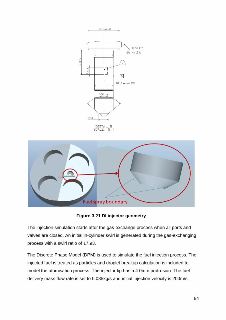
54
Figure 3.21 DI injector geometry
The injection simulation starts after the gas-exchange process when all ports and
valves are closed. An initial in-cylinder swirl is generated during the gas-exchanging
process with a swirl ratio of 17.93.
The Discrete Phase Model (DPM) is used to simulate the fuel injection process. The
injected fuel is treated as particles and droplet breakup calculation is included to
model the atomisation process. The injector tip has a 4.0mm protrusion. The fuel
delivery mass flow rate is set to 0.035kg/s and initial injection velocity is 200m/s.

55
In order to consider the movement of the piston and exhaust valves, a layering
dynamic mesh is applied. The hex/wedge type grid with 1~2mm internal grid size is
used in the CFD calculations.
3.5.1 Single injection
For single injection cases, the injection duration is set to 30° CA at 4000rpm. The in-
cylinder evaporated fuel mass is also recorded, as shown in Figure 3.22.
Figure 3.22 Mass of Evaporated Fuel
In all cases, the speed of fuel evaporation increases during the injection process.
After the end of injection, the liquid fuel evaporating speed slows down. Faster fuel
evaporation takes place at retarded injection due to higher charge temperature.
The main cause for the less total fuel vapour from the early injection cases is the fuel
film effect. Because of the in-cylinder swirl and lower charge density during the
earlier injection, the fuel spray has more chance to reach the cylinder wall and form a
liquid fuel film there, as shown in Figures 3.23 and 3.24.
0.00E+00
5.00E-06
1.00E-05
1.50E-05
2.00E-05
2.50E-05
3.00E-05
255 270 285 300 315 330 345 360
Mass o
f F
uel
Ev
ap
ora
ted
(kg
)
Crank Angle (DATDC)
SOI-255°ATDC
SOI-270°ATDC
SOI-285°ATDC
SOI-300°ATDC

56
Figure 3.23 The liquid fuel
distribution
Figure 3.24 Liquid fuel location against
radial coordination of CFD model
3.5.2 Split Injections
To improve the fuel injection and mixing quality, split injection simulation was then
carried out.
First, a simulation was performed to investigate the difference in performance
between single injection and split injection. The injection timing is shown in Figure
3.25. When a single injection is used, the injection starts from 240°ATDC and lasts
for 30°CA. During the split injection operation, fuel is delivered in two injections of
15°CA duration each. The dwell angle between the two injections is set to 10°CA.
The initial in-cylinder condition is the same as the single injection operation with an
initial swirl ratio of 17.93.

57
Figure 3.25 Injection Timing Sequence
As shown in Figure 3.26, the overall fuel evaporation is improved by the split
injection. Due to reduced momentum of each injection of shorter duration, there is
less chance for the liquid fuel to reach the piston, resulting in a more homogeneous
mixture.
Figure 3.26 Injection Timing Sequence
Since early injection has more chance to produce the fuel film, the effect of first
injection quantity has also been studied. As Figure 3.27 shows, the total fuel
evaporation is improved as the percentage of the first injection is reduced from 50%
to 20% despite the drop in fuel evaporation rate in the first injection.
0.00E+00
5.00E-06
1.00E-05
1.50E-05
2.00E-05
2.50E-05
3.00E-05
3.50E-05
4.00E-05
240 260 280 300 320 340 360
In-C
ylin
de
r e
vap
ora
ted
fue
l(kg
)
Crank Angle(°CA)
Single
Split
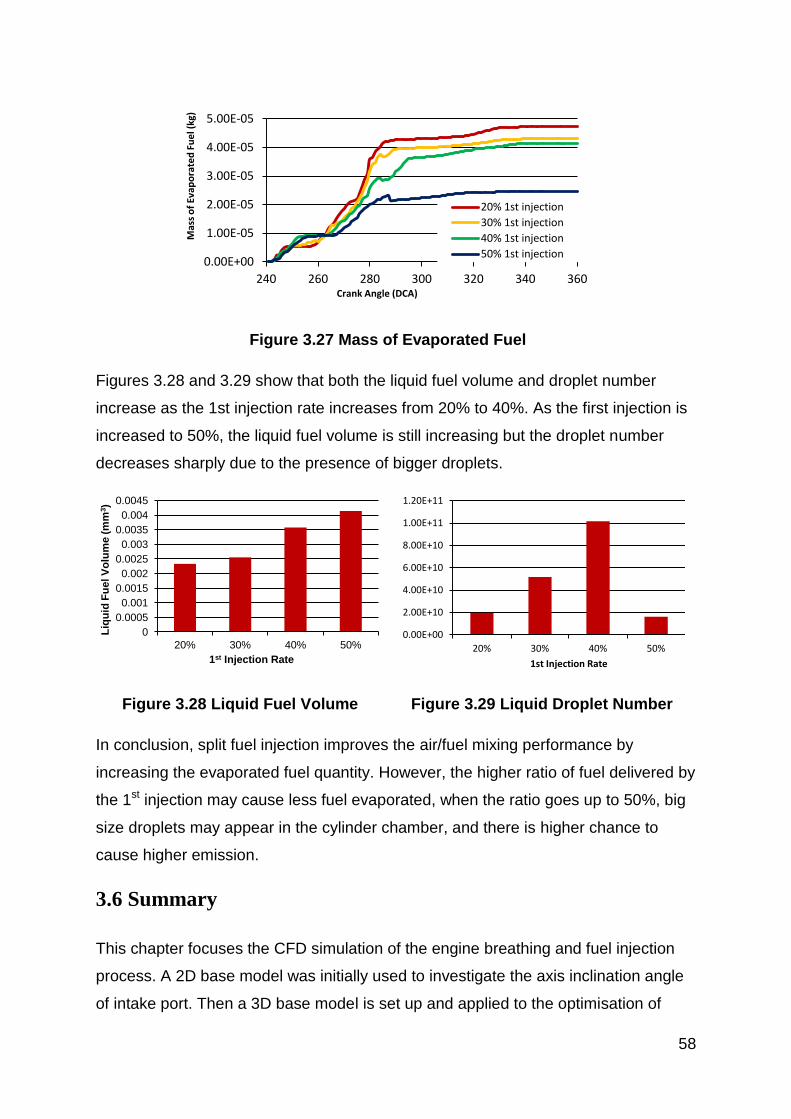
58
Figure 3.27 Mass of Evaporated Fuel
Figures 3.28 and 3.29 show that both the liquid fuel volume and droplet number
increase as the 1st injection rate increases from 20% to 40%. As the first injection is
increased to 50%, the liquid fuel volume is still increasing but the droplet number
decreases sharply due to the presence of bigger droplets.
Figure 3.28 Liquid Fuel Volume Figure 3.29 Liquid Droplet Number
In conclusion, split fuel injection improves the air/fuel mixing performance by
increasing the evaporated fuel quantity. However, the higher ratio of fuel delivered by
the 1st injection may cause less fuel evaporated, when the ratio goes up to 50%, big
size droplets may appear in the cylinder chamber, and there is higher chance to
cause higher emission.
3.6 Summary
This chapter focuses the CFD simulation of the engine breathing and fuel injection
process. A 2D base model was initially used to investigate the axis inclination angle
of intake port. Then a 3D base model is set up and applied to the optimisation of
0.00E+00
1.00E-05
2.00E-05
3.00E-05
4.00E-05
5.00E-05
240 260 280 300 320 340 360
Mas
s o
f Ev
apo
rate
d F
ue
l (kg
)
Crank Angle (DCA)
20% 1st injection
30% 1st injection
40% 1st injection
50% 1st injection
0
0.0005
0.001
0.0015
0.002
0.0025
0.003
0.0035
0.004
0.0045
20% 30% 40% 50%
Liq
uid
Fu
el V
olu
me (
mm
3)
1st Injection Rate
0.00E+00
2.00E+10
4.00E+10
6.00E+10
8.00E+10
1.00E+11
1.20E+11
20% 30% 40% 50%
1st Injection Rate

59
intake port swirl orientation angle and the port number. The injector feature was then
applied to the model. Finally the fuel injection strategy was investigated and the split
injection was shown to improve the fuel evaporation and mixture quality.

60
Chapter 4 Prediction of the Uniflow 2-Stroke
Engine Performance
4.1 Introduction
Although 3D CFD simulation is able to provide a wide range of information on engine
performance on a three-dimensional basis, 1D simulation is still used for engine
performance prediction because of its advantages of fast computation, high flexibility,
and adaptability of the model for the complete range of engine operation points.
For most of the cases in engine research, the 1D simulation code is developed
precisely for engine performance prediction. The code must be able to provide a fully
integrated treatment of time-dependent fluid dynamics and thermodynamics by
means of a one-dimensional formulation which enables performance simulations on
dynamics of pressure waves, mass flows, and energy losses in ducts, plenums, and
the manifolds of various systems.
A 1D thermo-fluid dynamic numerical code has been applied to the modelling of a
modern four-cylinder, turbocharged Diesel engine [63]. The results of average
quantities and the pressure pulsations along the ducts, the transient response of the
engine and the EGR system performance has been analyzed and resulted in
satisfactory agreement with measured data for every operating point considered,
showing the good quality of the 1D modelling. Research work has also been
dedicated to the development and validation of an advanced 1D thermo-fluid
dynamic model for the simulation of a single cylinder hydrogen SI engine [68]. The
comparison between measurements and computations of this research work has
pointed out a satisfactory agreement for most of the operating points considered,
with a good reliability of the adopted models in the studied range of operating
conditions and engine configurations.
The comparison between measurements and computations of this research work
has pointed out a satisfactory agreement for most of the operating points considered,
with a good reliability of the adopted models in the studied range of operating
conditions and engine configurations.

61
The model and simulation environment for the work described in this article is
RICARDO WaveBuild 8.3.2. WAVE is the 1D gas dynamics and engine simulation
software package. It is a computer-aided engineering code developed to carry out
simulations based on virtually any intake, combustion and exhaust system
configuration.
4.2 1D Engine Model Setup
WAVE is a 1D gas dynamics and engine simulation software package and is capable
of analyzing the dynamics of pressure waves, mass flows, and energy losses in
ducts, plenums, and the manifolds of various systems and machines. It provides a
fully integrated treatment of time-dependent fluid dynamics and thermodynamics by
means of a one-dimensional formulation which enables performance simulations to
be carried out based on virtually any intake, combustion and exhaust system
configuration [68].
Three baseline engine models were created, including a 1.6L naturally aspirated 4-
stroke engine, a 2-stroke 3-cylinder model and a 2-stroke 2-cylinder model
respectively shown in Figure 4.1. The 4-stroke engine was chosen as the bench
mark for the other uniflow 2-stroke engines.

62
1.6L 4 –stroke NA engine model
2-stroke 3-cylinder engine model
Figure 4.1 Baseline 1D engine models

63
2-stroke 2-cylinder engine model
Figure 4.1 (cont.) Baseline 1D engine models
Each engine model comprises
Inlet environment boundary
Intake system
Engine body
Boost system
Exhaust system
Outlet environment boundary
In this case, both inlet and outlet environment is set to be ambient at 1bar pressure
and temperature of 300K. The initial fluid composition is defined as fresh air. The
solution type is set to fixed boundary pressure, temperature and composition during
the simulation.
For the intake system, a butterfly plate in an orifice is used to represent the throttle
as shown in Figure 4.2. The orifice bore diameter is 50mm.Butterfly plate shaft
diameter is 6mm.

64
Figure 4.2 Throttle element structure
The intercooler system in the intake system is represented by a long pipe work at the
upstream side of intake manifold. The pressure drop along the pipe work is
calculated by Equation 4.1
[E-4.1]
Where
– Pressure drop along the pipe
– Velocity at the cell centre
– Area at the cell centre
– Length of the cell
– Resistivity of the absorptive material
And the heat transfer between the pipe wall and the inner gas is calculated by
Equation 4.2.
[E-4.2]
Where
– Heat transfer between pipe wall and inner gas
– Heat transfer multiplier constant
– Heat transfer coefficient

65
– Wall surface area
– Wall temperature
– Inner gas temperature
The heat transfer coefficient is calculated by
[E-4.3]
Where
– Conductivity of the wall
– Feature diameter of pipe wall
– Reynolds number
– Prandtl number
Engine body element defines the main engine configurations, such as engine bore,
stroke, cylinder number, firing sequence etc., and governs main calculations on
performance, such as friction losses calculation, scavenge governing profile
combustion model and etc. Also the valve lift profile and flow coefficient are defined
in the engine body element.
In the 4-stroke engine, the engine breathing model is defined and calculated by the
flow through the valves. In the case of the uniflow 2-stroke model, the gas
exchange and scavenging processes are defined by the flow coefficient of exhaust
valves and a pseudo intake valve, and a scavenge profile model.

66
Figure 4.3 Base valve lift profile of uniflow 2-stroke engine model
As shown in Figure 4.3, the lift profile and timing of the pseudo intake valve is
specified according to the port geometry and its relative location to the piston. The
flow coefficient of the gas flow through the valves is calculated as follows,
[E-4.4]
Where
– Flow coefficient
0
2
4
6
8
10
12
14
0 90 180 270 360
Val
ve L
ift[
mm
]
Crank Angle [ºCA]
Intake valve lift[mm]
Exhaust valve lift[mm]
Figure 4.4 Valve flow coefficient of uniflow 2-stroke model
0
0.1
0.2
0.3
0.4
0.5
0.6
0.7
0.8
0.9
1
0 0.1 0.2 0.3 0.4 0.5 0.6 0.7
Flo
w C
oe
ffic
ien
t
Lift/Diameter
Intake Valve Flow Coefficient
Exhaust Valve Flow Coefficient

67
– The effective area of the valve
– Valve reference diameter
– Valve lift
By setting the engine and valve configuration to the same as the 3D CFD calculation
model, the flow coefficient can be calibrated. The flow coefficient calibrated and
applied in the uniflow 2-stroke engine model is shown in Figure 4.4.
The scavenge model is based on tracking of residual and fresh mass in the
cylinder. At EVO, the entire contents are initialized to residual mass, and as fresh
charge enters, the incoming mixture is counted as the fresh mass. The scavenge
model contains a thermal mixing model that assumes that the fresh gas will gradually
mix with the exhaust gas during the scavenging event. It is set to heat up the fresh
gas to the cylinder-average gas temperature as the mass in the fresh zone reaches
100% of the cylinder contents. The scavenging curve represents the instantaneous
composition flowing through the exhaust valve as a function of instantaneous in-
cylinder composition. The scavenge curve is shown below in Figure 4.5. BR
(COMBUSTION CHAMBER) represents the burned mass fraction of the cylinder
contents, it will be 1.0 after combustion (100% combustion products) and decreases
toward zero as fresh air enters during the intake process. BR (EXHAUST STREAM)
is the instantaneous composition of the flow through the exhaust valve. When the
composition of the cylinder is 100% combustion products, the exhaust stream must
also be 100% products. Likewise, if the cylinder contains 100% fresh air, the
exhaust stream must also be 100% fresh air. Therefore, any scavenging curve must
move from the top right corner (1.0, 1.0) to the lower left corner (0.0, 0.0) of the
profile. Between these points, the curve can take any shape. When BR (EXHAUST
STREAM) is 1.0 according to the scavenging curve, perfect displacement
scavenging is occurring, fresh air entering the cylinder pushes out exhaust gases,
while no fresh air leaks out of the cylinder. When BR (EXHAUST STREAM) is 0.0,
complete short-circuiting is occurring, any exhaust gas in the cylinder is trapped
while fresh air blows out the exhaust valve. When BR (EXHAUST STREAM) equals
BR (COMBUSTION CHAMBER), a perfectly mixed scavenging is occurring: the
exhaust stream has the same composition as the combustion chamber’s average
contents [68].

68
Figure 4.5 Scavenge profile
After the flow coefficient applied, a single cylinder model has been used for a
simulation with same engine configuration as the 3D CFD model. The gas-exchange
performance has been compared and validated between 1D and 3D mode. As
shown in Figure 4.6, there is good agreement between 1D and 3D models. In most
cases, the differences are less than 5%. The maximum difference of 8.93% appears
with the trapping efficiency at 2000rpm but the absolute difference is rather small.
Thus, 1D calculations of gas-exchange and scavenging performance are considered
to be acceptable.

69
Engine Speed – 1000rpm
Engine Speed – 2000rpm
Engine Speed – 3000rpm
Engine Speed – 4000rpm
Figure 4.6 Gas-exchange performance of 3D and 1D models
0.00%
100.00%
200.00%
300.00%
400.00%
DR SE TE CE
3D CFD Model
1D Model
0.00%
50.00%
100.00%
150.00%
200.00%
DR SE TE CE
3D CFD Model
1D Model
0.00%
20.00%
40.00%
60.00%
80.00%
100.00%
120.00%
DR SE TE CE
3D CFD Model
1D Model
0.00%
20.00%
40.00%
60.00%
80.00%
100.00%
DR SE TE CE
3D CFD Model
1D Model

70
The Wiebe function is used to describe the heat release process of
combustion. This relationship allows the independent input of function shape
parameters and of burn duration. It is based on calculation of the cumulative mass
of burned fraction [68]
[E-4.5]
Where
– Internally calculated parameter to allow covering the range of 10%-90%
– Combustion duration (10%-90%)
– Degrees past start of combustion
– The exponent in Wiebe function
Since the calculation of the brake engine output needs to take into account of
frictional losses, the engine friction model in the 1-D engine simulation model was
set up and calibrated. Calculation of the frictional losses is based on Flynn-Chen
model [70],
[E-4.6]
Where
– Peak in-cylinder pressure
– Constant used to replicate the FMEP values determined by engine
experiments and then used to calculate FMEP at different load and speeds
The constants, in Equation 4.6 were determined based on the
engine friction data of Mahle I3 DI gasoline engine, which represents one of the most
advanced boosted DI gasoline engines, because this engine has similar
configurations with the 2-stroke engine model. In order to determine the constants in
Flynn-Chen model, a quadratic curve was created according to Equation 4.6, the
experimental data of the Mahle I3 DI gasoline engine such as engine speed, peak in-
cylinder pressure and etc. were imported, by solving the quadratic functions with

71
experimental data, the constants in Flynn-Chen model were determined. The
calibration results are shown in Figure 4.7 with values of is given in
0.35bar, 0.005, 10pa.min/m and 6pa.min2/m2 respectively.
Figure 4.7 FMEP calibration of 2-stroke engine model
4.3 1D Engine Simulation Results
The fuel mass flow rate of the 1D model was calculated according to the
stoichiometric air to fuel ratio of 14.7:1. In the spark ignition Wiebe heat release
model, the combustion duration (10% to 90% mass fraction burned) was set to
31°CA according to previous simulations. The 50% mass fraction burned angle,
CA50º, was varied to control the combustion phase. Figure 4.8 shows the timing
sequence of the 2-stroke cycle operation. The intake port opening and closing are
represented by IPO and IPC respectively and DIP is the duration of intake ports
opening. The exhaust valves open at EVO and closes at EVC. DEV is the duration of
exhaust valves opening period. The period between EVO and IPO defines the blow-
down duration, BDD. Fuel was injected directly into the cylinder after both the intake
ports and exhaust valves were closed to avoid the fuel short-circuiting.
4
6
8
10
12
14
16
1000 2000 3000 4000 5000 6000
Fri
ctio
n T
orq
ue
[Nm
]
Speed [rpm]
Friction Torque - MAHLE I3 Vs
Quadratic Fit
Friction Torque - 1D Calculation Modle

72
Figure 4.8 The timing sequence of 2-stroke operation
4.3.1 Effect of Engine Geometry on Performance
The previous 3D CFD simulation was focused on the engine breathing performance
optimisation and in-cylinder charge flow structure generation in the single cylinder
uniflow 2-stroke engine and to be compared with the experimental results. In order
to carry out a systematic evaluation of the boosted uniflow 2-stroke engine, 1D
simulation has been used to optimise the bore and stroke ratio for maximum engine
performance.
The first series of 1D engine performance simulation studies were carried out on a 3-
cylinder uniflow 2-stroke engine. The absolute boost pressure was set to 2bar,
engine speed at 4000rpm and CA50 at 15°ATDC. The intake port opening (IPO) was
set at 90°ATDC and blow-down duration of 60°CA.
The engine delivery ratio, trapping efficiency, and charging efficiency is shown in
Figures 4.9 to 4.11. The long engine stroke results in reduced engine delivery ability
but higher trapping efficiency because of the longer path of the fresh charge. The
charging efficiency is a combination of delivery ratio and trapping efficiency. The
higher the charging efficiency, the more power can be produced from the combustion
of a larger amount of air/fuel mixture. Thus, according to the charging efficiency
results in Fig.4.11, the best performance can be obtained in the engine of a shorter
stroke and bigger bore.

73
Figure 4.9 Delivery ratio at IPO – 90°ATDC , BDD – 60°CA
Figure 4.10 Trapping efficiency at IPO – 90°ATDC , BDD – 60°CA

74
Figure 4.11 Charging efficiency at IPO – 90°ATDC , BDD – 60°CA
As shown in Figure 4.12, at a given stroke of 80mm the highest specific indicated
power of the 3-cylinder uniflow 2-stroke engine can reach 78kW/L for larger
bore/stroke ratios.
Figure 4.12 Specific indicated power at IPO – 90°ATDC , BDD – 60°CA, CA50
- 15º ATDC
The results in Figure 4.12 can be explained by the trade-off between the scavenging
performance and expansion work. For a given bore/stroke ratio and IPO, the shorter
stroke results in a reduced intake port opening period and the fresh charge mass

75
flow rate is insufficient to scavenge the residual gas out of the cylinder, which leads
to a relatively low charging efficiency and hence lower power. Conversely, a longer
stroke extends the intake opening period and improves the gas-exchange
performance. However, with a long intake port opening duration and blow-down
duration, the effective expansion stroke is reduced, thus the output power is limited
with longer stroke. Therefore, the highest power output is achieved at an
intermediate stroke of 80mm.
The combustion phase also has an effect on engine output power. The results
shown in Fig.4.12 were obtained with CA50 set to 15º ATDC. When the CA50 was
advanced to 5º ATDC (Fig.4.13), the best performance zone was shifted up to an
area of longer stroke around 80mm and the bore/stroke ratio of the best performance
zone was extended. But the engine peak specific indicated power remained the
same.
Figure 4.13 Specific indicated power at IPO – 90°ATDC , BDD – 60°CA, CA50
- 5º ATDC
In order to reach the same power output as the 1.6L 4-stroke baseline engine, a
higher boost pressure than 2bar would be required. As shown in Fig.4.14, when
the boost pressure was increased to 3bar, the peak specific indicated power could
reach 121kW/L.

76
Figure 4.14 Specific indicated power at IPO – 90°ATDC , BDD – 60°CA, CA50
- 5º ATDC
4.3.2 Effect of the Blow-down Duration
The intake port timing is determined by the intake port location in a uniflow 2-stroke
engine. For a given intake port design, the intake port timing is fixed. The exhaust
valves are driven by a camshaft and can be altered through a variable valve timing
device. The optimised exhaust valve timing is a compromise between the gas-
exchanging performance and output power. With a longer blow-down duration and
hence less air short-circuiting, a higher trapping efficiency can be achieved. However,
for a fixed IPO timing, longer blowdown duration means the exhaust valves need to
be opened earlier, resulting in less expansion work and output power.
Figures 4.15 to 4.17 show the specific indicated power maps with intake port
openings at 110°ATDC, 120° ATDC, and 130° ATDC, respectively. The CA50 was
set to 5º ATDC and the intake pressure at 3bar. In light of the higher boost pressure
applied, the blow-down duration was reduced from 60°CA to 40°CA for greater
expansion work.

77
Figure 4.15 Intake port opening - 110°ATDC
Figure 4.16 Intake port opening – 120°ATDC

78
Figure 4.17 Intake port opening - 130°ATDC
It can be seen that the maximum specific indicated power can reach 170kW/L. In the
case of IPO at 110°ATDC, the best output performance was achieved with a higher
bore/stroke ratio and shorter stroke. As the IPO was retarded to 120°ATDC, the high
performance range was extended further, because of the increased effective
expansion stroke. When the IPO timing was retarded further to 130°ATDC, the
specific indicated power became lower because of the shorter intake port opening
duration and hence reduced intake charge mass flow rate.
As the specific indicated power was increased, the corresponding in-cylinder peak
pressure became very high. To reduce the peak pressure, the combustion phase
was retarded by changing CA50 from 5°ATDC to 15°ATDC. IPO timing was kept at
120°ATDC and blow-down duration of 40°CA. As shown in Figure 4.18, the peak
pressure was reduced by 25% with the retarded combustion phasing. As shown in
Figure 4.19, the peak cylinder pressure was below 120bar when the specific
indicated power was over 160kW/L.
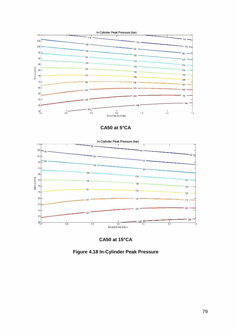
79
CA50 at 5°CA
CA50 at 15°CA
Figure 4.18 In-Cylinder Peak Pressure

80
Figure 4.19 Specific indicated power output at 4000rpm, 3 bar boost, and
CA50 at 15 CA ATDC
Figure 4.20 shows the effect of the blow-down duration on the brake specific power
output at different engine speeds.
Figure 4.20 Effect of blowdown duration on specific brake power output with
3 bar boost
At lower engine speeds, as the blowdown duration decreased, the brake specific
power increased. However, for engine speeds above 3000rpm, the brake specific

81
power increased initially with shorter blowdown duration and then decreased as the
blowdown duration became less than 50º CAs. Maximum power output was reached
when a balance between the trapping efficiency and charge efficiency was reached.
Therefore, it would be desirable that a variable valve timing device can be used to
alter the exhaust valve timing for different engine operating conditions.
4.3.3 Engine Packaging
The target of this research work is to evaluate the potential of the uniflow 2-stroke
engine to replace a bigger 4-stroke engine in a passenger car. Therefore it is
necessary to consider the dimension of the uniflow 2-stroke engine in the context of
the vehicle packaging requirement.
A typical practical engine packaging restriction in a VW Golf sized vehicle is shown
in Figure 4.21. As shown in figure 4.21, another vertical length will be added to
engine block, because of the valve driven system. And the above simulation shows
the best engine output performance can be achieved with 80mm engine stroke.
However, with 80mm engine stroke, the overall engine height including the valve
driven system (198mm) will be 438mm, which will exceed the restriction by 36mm.
By reducing the engine stroke down to 67mm, the engine overall height will be
brought down to 406mm, which is only 4mm more than the engine restriction and is
deemed acceptable.

82
Figure 4.21 Vehicle application packaging restrictions
Figure 4.22 Engine size determination
Taking into account of the engine packaging requirement and the cylinder head
space required for centrally mounted injector and spark with 4 exhaust valves, it is
decided that each cylinder will have a bore and stroke of 76mm x 67mm, giving a
displacement volume of 0.3L, as indicated by the red dot. Therefore, a 3-cylinder
uniflow 2-stroke engine of 0.9 litre capacity will be able to produce more than 150kW

83
indicated power at 4000rpm with the intake port opening set to 120°ATDC, much
greater than the 1.6 litre 4-stroke engine.
4.4 Summary
3D CFD simulation has been used for the optimisation of the engine breathing
process through the intake port design. In addition, the 3D CFD flow results were
used to provide the intake flow data for the subsequent 1D calculations. In order to
determine the frictional losses, the Flynn-Chen model was adopted to calculate the
engine FMEP and the coefficients in the model were determined from a state-of-art
gasoline engine.
Based on the 1D simulation result and engine packaging requirements, a 3-cylinder
uniflow 2-stroke engine of 0.9 litre capacity and a 2-cylinder version of 0.6L capacity
were selected for the subsequent vehicle simulations. The engine has a bore of
76mm and stroke of 67mm. The intake port opening time is set to 120ºATDC and the
intake port closing time is set to 240ºATDC. The exhaust valve opening and closing
time are 80ºATDC and 240ºATDC respectively.

84
Chapter 5 Optimisation of the Boost System for
the Uniflow 2-Stroke Engine
5.1 Introduction
In Chapter 4, potential performance of the boosted uniflow scavenged direct injection
gasoline (BUSDIG) 2-stroke engine was predicted for different stroke and bore
combinations. The intake air was boosted to achieve the target torque and power
output, limited by the maximum in-cylinder pressure of 120bar. In this chapter, the
boost system and engine interactions were examined to determine the appropriate
boosting arrangement for maximum performance and minimum fuel consumption.
Then, the vehicle driving cycle analysis is carried out to determine the fuel economy
benefit of the optimised BUSDIG engine system.
5.2 Modelling of the Boosted Engine and Vehicle Simulation
Model
The boost system comprises a turbocharger and/or a supercharger. The
supercharger is defined by a single performance map whilst the turbocharger
performance is determined by both the turbine and compressor performance maps,
which are characterised by the mass flow, pressure ratio, rotational speed and
efficiency. The physic model assumes that the flow in the boost system elements
behave in a quasi-steady manner and calculates the mass flow and enthalpy rise
across the elements as well as the torque produced by the elements or used to
driven the elements by interpolating a lookup map of steady state performance
behaviour.
Four basic parameters are required to define the maps: dimensionless speed,
dimensionless mass flow, dimensionless torque coefficient and blade speed ratio.
The parameters are defined as follow [71],

85
[E-5.1]
[E-5.2]
[E-5.3]
[E-5.4]
Where
– Dimensionless speed
– Dimensionless mass flow
– Dimensionless torque coefficient
– Blade speed ratio
– Rotational speed
– Reference diameter
– Gas constant
– Mass flow
– Inlet temperature
– Inlet pressure
– Shaft torque
– Specific heat of the gas
– Special heat capacity ratio
During the calculation, the pressure ratio, dimensionless speed and blade speed
ratio are calculated first and then used to interpolate the dimensionless mass flow
and torque coefficients and efficiency from the maps. The dimensionless mass flow
and torque coefficients can then be used to calculate the instantaneous mass flow,

86
torque, and the enthalpy rise of the compressor. The turbine power generated or
compressor work consumed is calculated as follows,
[E-5.5]
[E-5.6]
Where
– Power generated by the turbine
– Power consumed by the compressor
– Isentropic efficiency of an element
– Pressure Ratio
When the operating point of the elements is beyond the boundaries of the map,
extrapolation is applied, as shown in Figure 5.1.
Figure 5.1 Boost elements map extrapolation
The calculation results of boosted engine models were then exported to a vehicle
model to carry out calculations based on new European driving cycle (NEDC). The
baseline vehicle model parameters are shown in Table 5.1 based on a VW Golf.
The vehicle drag force in the vehicle model can be calculated as follows,

87
[E-5.7]
Where
– Aerodynamic drag coefficient
– Air density
– Vehicle speed relative to air
– Vehicle frontal area
Table 5.1 Baseline vehicle parameters
Vehicle data
Units Value
Vehicle mass kg 1157
Passenger and cargo mass kg 100
Frontal area m2 2.3
Aerodynamic drag coefficient 0.3
Tyre data
Units Value
Tyre rolling resistance 0.015
Tyre rolling radius m 0.3
The tyre rolling resistance force is calculated as follows,
[E-5.8]
Where
– Tyre rolling resistance factor
– Vehicle mass
– Passenger and cargo mass
– Gravitational
The rotation inertia of the elements set up is shown in Table 5.2.
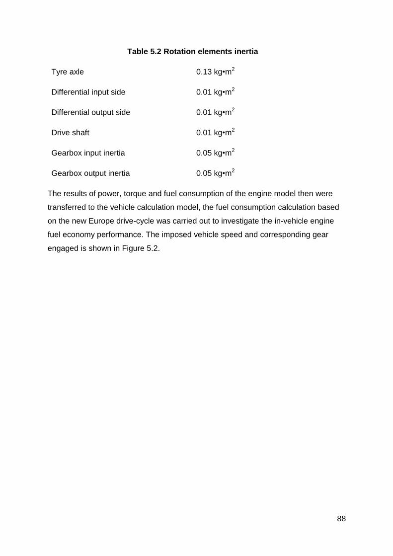
88
Table 5.2 Rotation elements inertia
Tyre axle 0.13 kg•m2
Differential input side 0.01 kg•m2
Differential output side 0.01 kg•m2
Drive shaft 0.01 kg•m2
Gearbox input inertia 0.05 kg•m2
Gearbox output inertia 0.05 kg•m2
The results of power, torque and fuel consumption of the engine model then were
transferred to the vehicle calculation model, the fuel consumption calculation based
on the new Europe drive-cycle was carried out to investigate the in-vehicle engine
fuel economy performance. The imposed vehicle speed and corresponding gear
engaged is shown in Figure 5.2.

89
Imposed vehicle speed
Imposed gear engaged
Figure 5.2 The new Europe drive-cycle (NEDC) conditions
5.3 Analysis of Boosted uniflow 2-stroke engine operations
In order to set a reference to the optimisation calculation of boosted engine model, a
baseline 4-stroke engine of 1.6L capacity was set up. The valve lift and timing are as
shown in Figure 5.3. As shown in Figure 5.4, the CA50 was set to 5ºCA ATDC at this
stage and the combustion duration was 30ºCA.
0
20
40
60
80
100
120
140
0 200 400 600 800 1000 1200
Ve
hic
le S
pe
ed
[km
/hr]
Time [s]
0
1
2
3
4
5
6
0 200 400 600 800 1000 1200
Ge
ar E
nga
ged
Time [s]

90
Figure 5.5 shows the predicted full load performance curves of the baseline 4-stroke
engine model. The baseline 4-stroke engine delivers its maximum brake power of
79kW at 6000rpm and maximum brake torque of 140Nm at 5000rpm engine speed.
Figure 5.3 Valve timing and lift of 4-stroke baseline model
Figure 5.4 Combustion phase of the 4-stroke engine model
0
1
2
3
4
5
6
7
8
9
10
-90 0 90 180 270 360 450 540 630
Val
ve L
ift
[mm
]
Crank Angle [°]
Exhaust valve lift
Intake valve lift
Compression TDC
Exhaust TDC

91
Figure 5.5 Baseline engine model performance curve
5.3.1 2-stroke engine model set up
The first boosted 2-stroke engine modelled is a 0.9L 3-cylinder engine with a single
supercharger. Subsequently, a turbocharged version of the 2-stroke engine is
modelled. Figure 5.6 shows the 1D calculation base model layout with supercharger
and turbocharger. Compared to the 4-stroke NA model, the engine’s capacity is
downsized by 44%. The engine has a bore of 76mm and a stroke of 67mm as
determined before. The air/fuel ratio was regulated by the injector element in the
model and was set to 14.7/1 of mass for the trapped air/fuel ratio. The restriction of
120bar peak in-cylinder pressure was applied. The ambient boundary was set at
pressure of 1bar and temperature of 300K.
0
20
40
60
80
100
120
140
160
0
10
20
30
40
50
60
70
80
90
0 1000 2000 3000 4000 5000 6000 7000
Bra
ke T
orq
ue
[N
m]
Bra
ke P
ow
er
[kW
]
Engine Speed [rpm]
Power[kW]
Torque[Nm]

92
Model with supercharger
Model with turbocharger
Figure 5.6 2-stroke 1D calculation base model layout

93
The supercharger, Eaton R200GT or R410GT, and the turbocharger used to boost
the Mahle I3 engine was chosen as the boost elements for engine models, it is
because Mahle I3 engine has similar engine configuration and capacity to the 2-
stroke engine model. To fit the mass flow through the 2-stroke engine model, the
performance maps of the turbocharger have been rescaled. The mass flow rate of
the turbine TD04L4-F5 is expanded by 125% and the mass flow rate of the
compressor TF035-13TK3S shrunk by 65%. The performance maps of those boost
elements are shown in Figure 5.7 to Figure 5.10.
Figure 5.7 Eaton R200GT performance map

94
Figure 5.8 Eaton R410GT performance map
Figure 5.9 Rescaled turbine performance map

95
Figure 5.10 Rescaled compressor performance map
5.3.2 Prediction of Boosted uniflow 2-stroke engine full-load performance
In the case of supercharged engine operations, the supercharger is driven by the
crankshaft directly under a specified gear ratio. Figure 5.11 shows the maximum
brake power predicted of the 2-stroke engine boosted by R200GT with various gear
ratios. The results reveal that as the gear ratio is increased from 4 to 7, the engine
output reaches a maximum power of 56kW at 4000rpm. Further increase in the gear
ratio leads to a drop in the brake power output. As shown in Figure 5.12, the flow
rate of the supercharger R200GT reaches the high flow rate end boundary with gear
ratio 7 and cannot be increased further with higher gear ratios, limiting the amount
of fuel to be burned and hence the resulting mechanical work that can be produced
by combustion. In the meantime, the increase in the power used to drive the
supercharger at a higher gear ratio will reduce the net power output of the engine.
Thus, the combination of limited engine power output and increasing power required
to drive the supercharger causes the brake power output to drop beyond a gear ratio
of 7.

96
Figure 5.11 Full load brake power of engine model with R200GT
supercharger at 4000rpm engine speed.
Figure 5.12 R200GT supercharger working points at engine full load at 4000
rpm engine speed
35
40
45
50
55
60
Bra
ke P
ow
er
(kW
)

97
Figure 5.13 Power consumption by a R200GT supercharger and the
proportion to the engine indicated power at 4000rpm full load
operation
In order to increase the target output engine power, R410GT is then used. The
maximum mass flow rate of R410GT is 650kg/hr, nearly 300kg/hr higher than
R200GT.
Figure 5.14 Full load brake power of engine model with a R410GT
supercharger at 4000rpm engine speed.
0%
5%
10%
15%
20%
25%
30%
0
2
4
6
8
10
12
14
4 5 6 7 8 9 10 11 12
Pro
po
rtio
n o
f P
ow
er
Dra
ine
d b
y Sp
erc
har
ger
to E
ngi
ne
In
dic
ate
d P
ow
er[
%]
Po
we
r co
nsu
me
d b
y Su
pe
rch
arge
r[kW
]
Gear Ratio
Power drained by supercharger[kW]
Proportion of power drained by supercharger to the engine indicated power[%]
60
65
70
75
80
85
90
Bra
ke P
ow
er
[kW
]

98
Figure 5.15 R410GT supercharger working points at engine full load at 4000
rpm engine speed
Figure 5.16 Power consumption by R410GT supercharger and the proportion
to the engine indicated power at 4000rpm full load condition
0%
10%
20%
30%
40%
50%
0.00
10.00
20.00
30.00
40.00
50.00
4 5 6 7 8 9 10 11 12
Pro
po
rtio
n o
f P
ow
er
Dra
ine
d b
y Sp
erc
har
ger
to E
ngi
ne
In
dic
ate
d
Po
we
r[%
]
Po
we
r D
rain
ed
by
Spe
rch
arge
r[kW
]
Gear Ratio
Power drained by supercharger[kW]
Proportion of power drained by supercharger to the engine indicated power[%]
99
As shown in Figure 5.14, the brake power reaches a maximum value of 84kW with a
gear ratio 6. Figure 5.15 shows the working points of R410GT at 4000rpm engine
speed and full engine load. Similar to the supercharger R200GT, when the gear ratio
is increased higher than 7, the compressor is restricted by the maximum mass flow
boundary and the power consumption by the supercharger can go up to nearly 40%
of the engine indicated power, as shown in Figure 5.16. Therefore, gear ratio 6
shows the best compromise between the engine power output and the power
consumption by the supercharger.
As shown above, the supercharger consumed a large proportion of indicated power,
which leads to a poor engine overall efficiency. The turbocharger is driven by the
exhaust gas, theoretically, no power drained directly from the engine output, thus the
engine overall efficiency is higher, so is the engine brake power and torque.
Figure 5.17 shows the working point of the rescaled supercharger and turbocharger.
As described previously, the performance map of the turbine used was TD04L4-F5,
to fit the engine condition, the mass flow range was expanded by 125% and the
mass flow range of the compressor TF035-13TK3S shrunk by 65%. With the
rescaled compressor and turbocharger, the engine flow fits the elements’ high
efficiency range.

100
Working points of the compressor
Working points of the turbine
Figure 5.17 Working points of the compressor and turbine of the model

101
With the rescaled turbine and compressor, the maximum boost pressure was still not
higher than 3bar. The full load power and torque curves are shown in Figure 5.18.
The peak power reached 105kW at 4000rpm engine speed. Meanwhile the peak
torque reached 296Nm at 2000rpm, and keeps higher than 250Nm from 2000rpm to
4000 rpm.
Figure 5.18 Full load power and torque curves of the turbocharged model
Figure 5.19 shows the full load brake power and torque curves of the baseline 4-
stroke engine and boosted 2-stroke engine operations. The R200GT supercharged
2-stroke engine can match the torque output of the baseline 4-stroke engine up to
4000rpm but its maximum power is insufficient. With R410GT, the supercharged
uniflow 2-stroke engine can produce the same maximum power at 4000rpm as the
baseline 4-stroke engine at 6000rpm, and it is characterised with superior torque
output across the whole speed range of the 2-stroke engine operations. With the
rescaled turbocharger, both the engine power and torque target were substantially
exceeded. Actually, when it is equipped with the rescaled turbocharger, the uniflow
2-stroke engine exhibits extremely high torque and the target maximum power can
be reached at 2500rpm, which suggests that further downsizing of the 2-stroke
engine from 3-cylinder to 2-cylinder is a viable option.
0
50
100
150
200
250
300
350
0
20
40
60
80
100
120
0 1000 2000 3000 4000 5000
Bra
ke T
orq
ue
[Nm
]
Bra
ke P
ow
er[
kW]
Engine Speed[rpm]
Brake Power[kW]
Brake Torque[Nm]

102
Brake Power Brake Torque
Figure 5.19 Full load brake power and torque curves of all engines
5.3.3 Analysis of boosted uniflow 2-stroke engine operations
In order to compare the performance of all the engines modelled, some engine
operating conditions were chosen. The first engine operation point is the high speed
and high load operation of 4000rpm engine speed and 55kW brake power. As shown
in Figure 5.20, the 4-stroke NA engine has the highest charging efficiency despite
the boosted operation of all 2-stroke engines. Among the 2-stroke engine
configurations, the turbocharged operation exhibits the lowest charging efficiency
due to the higher back pressure in the exhaust manifold.
0
20
40
60
80
100
120 B
rake
Po
we
r[kW
]
Engine Speed[rpm] 2-Stroke Model Boosted By R200GT
2-Stroke Model Boosted By R410GT
4-Stroke Baseline Model
2-Stroke Model Boosted By Turbocharger
0
50
100
150
200
250
300
350
Bra
ke T
orq
ue
[Nm
]
Engine Speed[rpm]
2-Stroke Model Boosted By R200GT
2-Stroke Model Boosted By R410GT
4-Stroke Baseline Model
2-Stroke Model Boosted By Turbocharger

103
Figure 5.20 Charging efficiency of baseline 4-stroke and boosted 2-stroke
engines
Figure 5.21 shows the corresponding IMEP values of the baseline 4-stroke and
boosted uniflow 2-stroke engines. For a given power and torque output at the same
engine speed, the IMEP value of the 2-stroke engine operation is theoretically halved.
But the results in Figure 5.21 are significantly different from the theoretical values
because of the lower charging and trapping efficiency of the 2-stroke scavenging
process than the 4-stroke gas exchange as well as their smaller displacement
volume than the baseline engine. The higher power consumption by R410GT
requires more IMEP to be produced for the same brake power and torque output,
and hence the highest boost pressure as shown in Figure 5.22. Since it is the
pressure ratio between the intake and exhaust which determines the charging and
trapping efficiencies, higher exhaust back pressure are shown by the turbocharger.
As a consequence, the turbocharged operation leads to higher residual gas fraction
as shown in Figure 5.23.
0%
20%
40%
60%
80%
100%
120%
4-Stroke NA 2-Stroke R200GT 2-Stroke R410GT 2-Stroke Turbo

104
Figure 5.21 IMEP values at 4000rpm and 55kW
Figure 5.22 Intake and exhaust pressures at 4000rpm and 55kW
0
2
4
6
8
10
12
14
16
18
20
4-Stroke NA 2-Stroke R200GT 2-Stroke R410GT 2-Stroke Turbo
IMEP
[b
ar]
0
0.5
1
1.5
2
2.5
4-Stroke NA 2-Stroke R200GT 2-Stroke R410GT 2-Stroke Turbo
Pre
ssu
er
[bar
]
Intake Pressure Exhaust Pressure

105
Figure 5.23 Residual Gas Fraction at 4000rpm and 55kW
Figure 5.24 shows the breakdown analysis of engine output and losses of work. For
the 4-stroke baseline engine, 81.5% of indicated work is converted into the brake
work at the crank shaft output. The turbocharged 2-stroke operation has the highest
mechanical efficiency of 84% much higher than the supercharged 2-stroke
operations, due to the absence of power consumption by a supercharger.
As shown in Figure 5.25, the turbocharged 2-stroke engine shows the same specific
fuel consumption rate as the baseline 4-stroke engine. The 2-stroke engine with the
larger supercharger has the highest fuel consumption.
0
2
4
6
8
10
12
14
16
4-Stroke NA 2-Stroke R200GT 2-Stroke R410GT 2-Stroke Turbo
Re
sid
ual
Gas
Fra
ctio
n [
%]

106
Figure 5.24 Engine output breakdown analysis at 4000rpm and 55kW
Figure 5.25 BSFC at 4000rpm and 55kW
The high speed and medium load at 4000rpm and 35kW is the second operating
point chosen for comparison. As shown in Figure 5.26 to Figure 5.29, the same
relative performances at this operating condition are observed for the engine
charging efficiency, IMEP, intake and exhaust pressure and BSFC results as the
high load operation.
81.5% 75.9%
44.2%
84.0%
16.2% 15.5%
11.2%
16.0% 2.2% 8.7%
45.2%
0%
10%
20%
30%
40%
50%
60%
70%
80%
90%
100%
4-Stroke NA 2-Stroke R200GT 2-Stroke R410GT 2-Stroke Turbo
BMEP% Friction Lost[%] Pumping Lost[%] Power driven compressor[%]
0
0.1
0.2
0.3
0.4
0.5
0.6
4-Stroke NA 2-Stroke R200GT 2-Stroke R410GT 2-Stroke Turbo
BSF
C[k
g/kW
/hr]

107
Figure 5.26 Charging efficiency at 4000rpm and 35kW
Figure 5.27 IMEP at 4000rpm and 35kW
0%
10%
20%
30%
40%
50%
60%
70%
80%
90%
100%
4-Stroke NA 2-Stroke R200GT 2-Stroke R410GT 2-Stroke Turbo
0
2
4
6
8
10
12
14
16
18
4-Stroke NA 2-Stroke R200GT 2-Stroke R410GT 2-Stroke Turbo
IMEP
[bar
]

108
Figure 5.28 Intake and exhaust pressures at 4000rpm and 35kW
Figure 5.29 Residual Gas Fraction at 4000rpm and 35kW
However, as shown in Figure 5.30, the percentage of supercharger power increased
significantly as the load was decreased. In the case of R410GT, 61.8% indicated
power is used to drive the supercharger, resulting in the highest fuel consumption.
According to Figure 5.31, the baseline 4-stroke engine and the turbocharged 2-
stroke engine exhibit 10% increase in BSFC. In comparison, the two supercharged
2-stroke engines suffer a fuel consumption penalty of 51% and 62%, respectively.
0
0.5
1
1.5
2
2.5
4-Stroke NA 2-Stroke R200GT 2-Stroke R410GT 2-Stroke Turbo
Pre
ssu
er
[bar
]
Intake Pressure Exhaust Pressure
0
5
10
15
20
25
4-Stroke NA 2-Stroke R200GT 2-Stroke R410GT 2-Stroke Turbo
Re
sid
ual
Gas
Fra
ctio
n[%
]

109
Figure 5.30 Engine output breakdown analysis at 4000rpm and 35kW
Figure 5.31 BSFC at 4000rpm and 35kW
When the load is reduced to 10kW at 4000rpm, engine efficiencies drop further. As
Figure 5.32 shows, about 40% work is lost to friction in both the baseline 4-stroke
engine and the turbocharged 2-stroke engine as the indicated power becomes less.
In addition, the baseline 4-stroke engine incurs an additional 13.2% pumping losses.
In the case of supercharged engine operations, most of the engine work is used to
drive the supercharger, up to 74% with R410GT. A direct result is the fuel
consumption increases to a very high level as shown in Figure 5.33.
74.0%
50.6%
27.3%
77.1%
22.0%
17.5%
11.8%
22.9%
4.0%
32.3%
61.8%
0%
10%
20%
30%
40%
50%
60%
70%
80%
90%
100%
4-Stroke NA 2-Stroke R200GT
2-Stroke R410GT
2-Stroke Turbo
Power driven compressor[%]
Pumping Lost[%]
Friction Lost[%]
BMEP%
0
0.1
0.2
0.3
0.4
0.5
0.6
0.7
0.8
0.9
4-Stroke NA 2-Stroke R200GT 2-Stroke R410GT 2-Stroke Turbo
BSF
C[k
g/kW
/hr]

110
Figure 5.32 Engine output breakdown analysis at 4000rpm and 10kW
Figure 5.33 BSFC at 4000rpm and 10kW
Figure 5.34 to Figure 5.38 show the engine output breakdown analysis at 2000rpm
and 1000rpm and various loads. Similar to the results at 4000rpm engine speed, the
turbocharged 2-stroke engine shows similar mechanical efficiencies to the baseline
4-stroke engine, whilst the supercharged engines have to take high proportion of
engine output to drive the supercharger. In addition, it is noted that the baseline 4-
stroke engine is characterised with higher pumping losses at lower load than the
turbocharged 2-stroke engine.
46.7%
30.4%
14.6%
56.3%
40.2%
19.7%
12.4%
43.7%
13.2%
50.5%
74.0%
0%
10%
20%
30%
40%
50%
60%
70%
80%
90%
100%
4-Stroke NA 2-Stroke R200GT
2-Stroke R410GT
2-Stroke Turbo
Power driven compressor[%]
Pumping Lost[%]
Friction Lost[%]
BMEP%
0
0.2
0.4
0.6
0.8
1
1.2
1.4
1.6
4-Stroke NA 2-Stroke R200GT 2-Stroke R410GT 2-Stroke Turbo
BSF
C[k
g/kW
/hr]

111
Figure 5.34 Engine output breakdown analysis at 2000rpm, 20kW
Figure 5.35 Engine output breakdown analysis at 2000rpm, 10kW
87.6% 78.6%
55.4%
88.1%
10.8%
10.5%
8.2%
11.9% 1.6%
11.1%
36.9%
0%
10%
20%
30%
40%
50%
60%
70%
80%
90%
100%
4-Stroke NA 2-Stroke R200GT 2-Stroke R410GT 2-Stroke Turbo
BMEP% Friction Lost[%] Pumping Lost[%] Power driven compressor[%]
81.8%
47.8% 37.2%
82.6%
13.7%
11.9%
8.7%
17.4% 4.6%
40.8% 54.8%
0%
10%
20%
30%
40%
50%
60%
70%
80%
90%
100%
4-Stroke NA 2-Stroke R200GT 2-Stroke R410GT 2-Stroke Turbo
BMEP% Friction Lost[%] Pumping Lost[%] Power driven compressor[%]
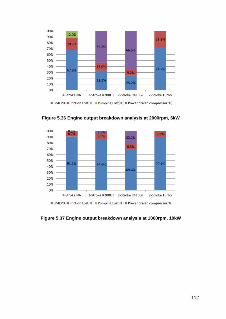
112
Figure 5.36 Engine output breakdown analysis at 2000rpm, 6kW
Figure 5.37 Engine output breakdown analysis at 1000rpm, 10kW
67.9%
33.5% 25.2%
71.7%
20.2%
13.0%
9.2%
28.3%
12.0%
54.3% 66.5%
0%
10%
20%
30%
40%
50%
60%
70%
80%
90%
100%
4-Stroke NA 2-Stroke R200GT 2-Stroke R410GT 2-Stroke Turbo
BMEP% Friction Lost[%] Pumping Lost[%] Power driven compressor[%]
91.1% 86.9%
69.6%
90.1%
8.7% 9.6%
8.5%
9.9% 0.2% 3.5%
22.2%
0%
10%
20%
30%
40%
50%
60%
70%
80%
90%
100%
4-Stroke NA 2-Stroke R200GT 2-Stroke R410GT 2-Stroke Turbo
BMEP% Friction Lost[%] Pumping Lost[%] Power driven compressor[%]

113
Figure 5.38 Engine output breakdown analysis at 1000rpm, 5kW
At the same engine speed and load, as shown in Figure 5.39, supercharged 2-stroke
engines incur much higher fuel consumption especially at part load and low load
conditions.
Figure 5.39 BSFC comparisons at the same speed and load conditions
between 4-stroke engine and 2-stroke engines
Because 0.9 litre 3-cylinder 2-stroke engines are capable of generating higher torque
outputs than the baseline 1.6 litre 4-cylinder 4-stroke engine, one possible way to
improve the 2-stroke engine’s fuel consumption during vehicle driving is engine
80.1%
57.7% 49.6%
83.9%
13.6%
11.1%
8.8%
16.1% 6.3%
31.6% 42.1%
0%
10%
20%
30%
40%
50%
60%
70%
80%
90%
100%
4-Stroke NA 2-Stroke R200GT 2-Stroke R410GT 2-Stroke Turbo
BMEP% Friction Lost[%] Pumping Lost[%] Power driven compressor[%]
0
0.2
0.4
0.6
0.8
1
1.2
1.4
1.6
4-Stroke NA 2-Stroke Turbo 2-Stroke R200GT 2-Stroke R410GT

114
downspeeding. Equation 5.9 shows the relationship between engine speed, power
and torque,
[E-5.9]
Where
– Engine power
– Engine speed
– Engine Torque
Thus, for the same engine power required to drive a vehicle, the engine operating
points can be shifted to higher torque and lower engine speed when the 2-stroke
engines are used.
Figure 5.40 BSFC at various engine speed and load.
Figure 5.40 compares the BSFC values of the baseline 4-stroke engine operating at
one and half times of the 2-stroke engines; i.e., 4-stroke 6000rpm vs. 2-stroke
4000rpm, 4-stroke 3000rpm vs. 2-stroke 2000rpm, and 4-stroke 1500rpm vs. 2-
stroke 1000rpm. The results reveal that the lower fuel consumption can be obtained
with the turbocharged 2-stroke engine operations than the baseline 4-stroke engine.
0
0.2
0.4
0.6
0.8
1
1.2
1.4
1.6
4-Stroke NA 2-Stroke Turbo 2-Stroke R200GT 2-Stroke R410GT

115
Furthermore, the 0.9litre turbocharged 3-cylinder 2-stroke engine model has been
shown to produce excess power and torque than the targeted maximum
performance of the baseline 4-stroke model. Thus, further downsizing of the
turbocharged 2-stroke engine can be exploited to reduce the engine fuel
consumption by reducing the engine to 0.6L capacity with two cylinders. The added
benefit of the 2-cylinder vs. 3-cylinder is the removal of interference in the exhaust
flows during the scavenging periods of adjacent cylinder when the exhaust duration
has to be over 120ºCA.
Figure 5.41 shows the full load brake power and torque curves of the baseline 4-
stroke engine, turbocharged 3-cylinder (0.9 litre) and 2-cylinder (0.6 litres) 2-stroke
engines. Although the power and load delivered by the 0.6L 2-stroke engine are
lower than the 0.9L 2-stroke engine, they are still higher than the baseline engine
and meet the vehicle’s performance requirement.
Brake Power Brake Torque
Figure 5.41 Full load brake power and torque of turbocharged 2-stroke
engines
Figure 5.42 shows that at the same engine speed and power, 0.6L turbocharged 2-
stroke engine shows better fuel consumption than the 0.9L 2-stroke model but is still
0
20
40
60
80
100
120
500 1500 2500 3500 4500 5500
Bra
ke P
ow
er[
kW]
Engine Speed[rpm]
2-Stroke Turbo-0.6L
4-Stroke Baseline Model
2-Stroke Turbo-0.9L
0
50
100
150
200
250
300
350
500 1500 2500 3500 4500 5500
Bra
ke T
orq
ue
[Nm
]
Engine Speed[rpm]
2-Stroke Turbo-0.6L
4-Stroke Baseline Model
2-Stroke Turbo-0.9L

116
poorer than the 4-stroke baseline engine at most of the points. However, Figure 5.43
shows that 0.6L 2-stroke engine shows the best fuel economy at most of the points
when the downspeeding is employed.
Figure 5.42 BSFC of the baseline 4-stroke and turbocharged 2-stroke
engines at the same speed and power
Figure 5.43 BSFC of the baseline 4-stroke and downspeeded 2-stroke
engines
0 0.05
0.1 0.15
0.2 0.25
0.3 0.35
0.4 0.45
0.5
4-Stroke NA 2-Stroke Turbo-0.9L 2-Stroke Turbo-0.6L
0
0.1
0.2
0.3
0.4
0.5
0.6
0.7
4-Stroke NA 2-Stroke Turbo-0.9L 2-Stroke Turbo-0.6L

117
Figure 5.44 plots the corresponding BSFC maps of the three engines as a function of
speed and load. In order to take into account of the downspeeding potential of the 2-
stroke operations, Figure 5.45 includes the revised BSFC map of the 4-stroke engine
which is rescaled to the speed range up to 4000rpm according to Equation 5.9. For
example, the 6000rpm and 75Nm point with 47.7kW brake power of the 4-stroke
model in Figure 5.44 is now shown as 4000rpm and 107.5Nm with same brake
power in Figure 5.45.
Figure 5.44 BSFC contours of the 4-stroke and turbocharged 2-stroke
engines
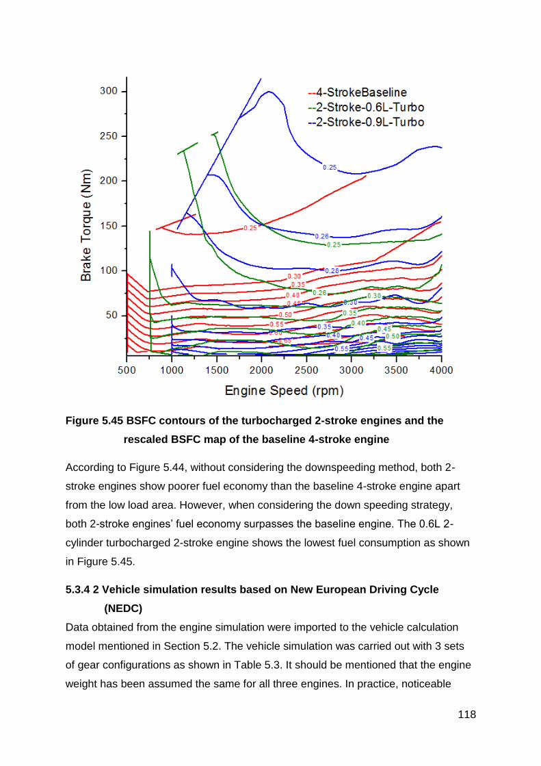
118
Figure 5.45 BSFC contours of the turbocharged 2-stroke engines and the
rescaled BSFC map of the baseline 4-stroke engine
According to Figure 5.44, without considering the downspeeding method, both 2-
stroke engines show poorer fuel economy than the baseline 4-stroke engine apart
from the low load area. However, when considering the down speeding strategy,
both 2-stroke engines’ fuel economy surpasses the baseline engine. The 0.6L 2-
cylinder turbocharged 2-stroke engine shows the lowest fuel consumption as shown
in Figure 5.45.
5.3.4 2 Vehicle simulation results based on New European Driving Cycle
(NEDC)
Data obtained from the engine simulation were imported to the vehicle calculation
model mentioned in Section 5.2. The vehicle simulation was carried out with 3 sets
of gear configurations as shown in Table 5.3. It should be mentioned that the engine
weight has been assumed the same for all three engines. In practice, noticeable

119
weight reduction from the 4-cylinder 4-stroke engine to the 2-cylinder turbocharged
2-stroke engine will be envisaged, which could benefit the vehicle’s fuel economy.
Table 5.3 Transmission gear ratio
Gear Ratio Setup Gear Mechanical Efficiency SET1 SET2 SET3
Number of gears 5 5 5
1st Gear ratio 0.95 5.4 3.6 2.4
2nd Gear ratio 0.96 3 2 1.33
3rd Gear ratio 0.97 2.025 1.35 0.9
4th Gear ratio 0.98 1.5 1 0.67
5th Gear ratio 0.97 1.2 0.8 0.53
Figure 5.46 shows the engine operating points during the vehicle’s NEDC calculation,
together with the full load torque curves of the baseline 1.6L 4-cylinder 4-stroke
engine, 0.9L 3-cylinder and 0.6L 2-cylinder turbocharged 2-stroke engines. With gear
set1, all engine operating points are covered for each of the three engines.
Figure 5.46 Engine operating points with gear set1 during NEDC and engine
full load torque curves
Figure 5.47 and Figure 5.48 show the engine operating points and the full load
curves of the engines with transmission gear set2 and set3, respectively. With down-
speeded gear set2, some of the high load engine points cannot be covered by the 4-
0
50
100
150
200
250
300
350
500 1500 2500 3500 4500 5500
Engi
ne
Bra
ke T
orq
ue
[Nm
]
Engine Speed[rpm]
2-Stroke Turbo-0.6L 2-Stroke Turbo-0.9L
4-Stroke Baseline Model Engine Working Points

120
stroke engine. This indicates that the gear set2 is beyond the down speeding
boundary of the 4-stroke engine. With gear set3, the engine operating points are
approaching the torque limit of the large 2-stroke engine whilst a significant
proportion of engine working points is out of the area covered by the baseline 4-
stroke engine.
Figure 5.47 Engine operating points with gear set2 during NEDC and engine
full load torque curves
0
50
100
150
200
250
300
350
500 1000 1500 2000 2500 3000 3500 4000 4500 5000 5500 6000
Engi
ne
Bra
ke T
orq
ue
[Nm
]
Engine Speed[rpm]
2-Stroke Turbo-0.6L 2-Stroke Turbo-0.9L
4-Stroke Baseline Model Engine Working Points

121
Figure 5.48 Engine operating points with gear set3 during NEDC and engine
full load torque curves
Figure 5.49 shows the average fuel consumptions of all three engines with the 3
gear sets during NEDC. The downspeeding strategy improves the fuel consumption
performance on all engines. However, because of their superior low speed torque,
the turbocharged 2-stroke engines have wider torque margin than the 4-stroke
engine and hence they can be down-speeded for better vehicle fuel economy. It can
be seen that the 0.6L 2-cylinder turbocharged 2-stroke engine with gear set3 delivers
6.91L/Km fuel consumption during NEDC, which improves the fuel consumption by
23.6% over the baseline 4-stroke engine.
0
50
100
150
200
250
300
350
0 1000 2000 3000 4000 5000 6000 7000
Engi
ne
Bra
ke T
orq
ue
[Nm
]
Engine Speed[rpm]
2-Stroke Turbo-0.6L 2-Stroke Turbo-0.9L
4-Stroke Baseline Model Engine Working Points

122
Figure 5.49 Average fuel consumption over NEDC
5.4 Summary
This chapter focuses on the 1D simulation of the engine performance and vehicle
fuel consumption simulations of three engines. They are the 1.6L 4-cylinder 4-stroke
NA engine as the baseline, a 0.9L 3-cylinder 2-stroke engine and a 0.6L 2-cylinder 2-
stroke engine with a supercharger or a turbocharger.
All simulations are focused upon engine steady state, the transient performance has
not been investigated. Because a high proportion of the engine output is used to
drive the supercharger, supercharged engines cannot meet the output target without
fuel economy penalties. Compare to a supercharger, a turbocharger is driven by the
exhaust energy that would otherwise be lost. The turbocharged 2-stroke engines
outperform the supercharged operations in both torque output and fuel consumptions,
though it increases the exhaust back pressure and the residual gas fraction in the
cylinder.
Because of its superior low speed torque, the turbocharged 2-stroke engine can be
operated at lower speeds with a lower gear ratio to maximize the downspeeding
potential. Combining downsizing and downspeeding, the 0.6L 2-cylinder
turbocharged 2-stroke engine delivers 23.6% less fuel consumption compared to the
baseline model without penalizing the engine power and torque output.
9.04 9.82
7.90 7.39
8.18 7.14 6.91
0
2
4
6
8
10
12
Gear Set1 Gear Set2 Gear Set3
L/1
00
Km
4-stroke baseline model 0.9L 2-stroke model 0.6L 2-stroke model

123
Chapter 6 Single Cylinder Uniflow 2-stroke
Engine and Experimental Facility
6.1 Introduction
In order to verify the simulation results and carry out preliminary experimental
investigation of the newly proposed Boosted Uniflow Scavenged Direct Injection
Gasoline (BUSDIG) engine concept, a single cylinder engine was modified to
operate as a uniflow 2-stroke direct injection gasoline engine. In this chapter, the
design and implementation of the modified engine is described in detail.
6.2 Uniflow 2-stroke engine setup
Figure 6.1 shows the layout of the newly designed engine assembly for the uniflow
2-stroke operation. A single cylinder Ricardo Hydra optical engine with a bespoke
four-valve DI gasoline cylinder head is used as the base engine. The engine is
mounted on a dedicated single cylinder engine test bed with integrated coolant and
oil cooling modules. The engine is driven by a McClure DC dynamometer with a
maximum speed of 6000rpm. The dynamometer is controlled by a separate control
console with a < ±5 rpm accuracy.
The original cylinder head is mounted above a glass ring. Beneath the glass ring,
there is a newly designed intake block assembly consisting of an intake channel
block (in Green) with embedded intake channels, an intake port block (in Blue) with
embedded intake ports on a specified orientation, and a new cylinder liner with holes
cut and aligned to the intake ports. The original engine extension block (in Brown)
and elongated piston with a crown window is designed to accommodate a 45º mirror
for in-cylinder optical access. A new longer timing belt is installed to drive both
camshafts with 2 tensioners. Details of the engine geometry are given in Table 6.1.
Further CAD drawings can be found in Appendix.

124
Figure 6.1 Uniflow 2-Stroke Single Cylinder Engine assembly layout

125
Table 6.1 Engine configuration
Combustion chamber Pent-roof
Displaced volume 450 cc
Bore 80 mm
Stroke 89 mm
Compression Ratio 8:1 to 12:1
Inlet valves diameters 29.5mm
Exhaust valves diameters 21mm
Valve lift 9mm
Valve opening duration 110ºCA
6.2.1 Cylinder Head
The cylinder head used for the experimental engine is a bespoke single cylinder
head machined from a single aluminium block by Orbital Engine Corporation Ltd. It
features a pentroof combustion chamber, a centrally located injector fitting hole and
a spark plug, as shown in Figure 6.2. Two independent camshafts actuate the two
intake valves and two exhaust valves. For the uniflow 2-stroke operation, all 4-valves
are used as exhaust valves. Since each camshaft is designed to produce a valve
opening period of 110ºCA, the exhaust period can be varied between 110ºCA to
220ºCA by adjusting the relative cam phasing. A pressure transducer is installed on
the cylinder head. In order to replace the air assisted injector with the piezo DI
injector, an adaptor was designed for the injector to fit the injector mounting slot. This
adaptor was designed for multiple injector usage. When another injector is required,
no more modification was required in the cylinder head, but only fitting the adaptor to
the injector.

126
Figure 6.2 Cylinder head layout
6.2.2 Optical window ring
The optical window ring is shown in Figure 6.3. The window ring is made of fused
silica and can withstand up to 50bar pressure. The ring sits into a seat with 3mm
depth grove. High temperature gaskets of 1.5mm are placed on both sides of the
glass ring to protect it from direct contact with the metal surfaces and provide the
sealing. The glass ring is mounted between the cylinder head and cylinder block by
means of 4 ring spacers positioned by the long cylinder head bolts and matched in
their height to that of the glass window plus the thickness of the gaskets below and
above the glass ring.

127
Figure 6.3 Optical window ring
6.2.3 Cylinder liner
The baseline 4-stroke Ricardo Hydra optical engine was designed with an extension
block to accommodate the elongated hollow piston for in-cylinder optical access
through the piston crown window via a 45 degree mirror mounted in the block. This
extension block was machined with an integrated cylinder liner. As shown in Figure
6.1, a new intake block is to be mounted above this original extension block and the
piston will need to travel inside both the new intake block and the original extension
block. In order to prevent piston rings from damage when moving across the
interface of these two blocks, a new longer liner was sourced from Mahler and
installed through both blocks.
As shown in Figure 6.4, the new one-piece cylinder liner was machined with six
windows in the top part, with three on opposite sides, which are aligned to the intake
ports in the intake port block.

128
Figure 6.4 New Cylinder Liner
6.2.4 Intake port block and intake channel block
The intake port block and intake channel block are required to allow the boosted air
into the combustion chamber. By having separate blocks, the geometry of the intake
ports can be altered with different intake port blocks in order to study the effect of
intake port design on in-cylinder flow and scavenging process. The intake port block
and intake channel block layout is shown in Figure 6.5. Along the interface between
the cylinder liner and intake port block, and also along the interface between the
intake channel block and intake port block, two O-ring groves are machined for high
temperature O-rings on both top and bottom sides to seal the intake path.

129
Figure 6.5 Intake port block and intake channel block layout
As shown in Figure 6.6, the intake port block is designed to provide the intake ports
of appropriate geometry according to the 3D CFD simulation studies. As discussed
in Chapter3, the intake ports affect the engine breathing performance directly, and
the orientation of intake ports also affect the in-cylinder flow swirl generating ability.
The 3D CFD simulation results suggested that the intake ports with 60º axis
inclination angle and 20º swirl orientation angle gave the best performance. The exit
of intake ports in the intake port block is aligned to the ports in the cylinder liner.

130
Figure 6.6 Intake port block configuration
Figure 6.7 shows the design of the intake channel block which connects the boosted
intake air to the intake ports. The block features two channels on each side of the
block and each channel is aligned to the 3 ports on one side of the intake port block.
Figure 6.7 Intake channel block configuration
6.2.5 Piston assembly
As shown in Figure 6.8, the piston assembly consists of a top piston part with a flat
optical window, a piston spacer and a piston extension part.

131
Figure 6.8 Piston assembly
The piston window is made of fused silica, same as the window ring. Along the side
surface of the piston window, high temperature silicon paste was applied to fill the
gap between the window and piston inner surface for sealing. High temperature
gaskets were placed below and above the window. The top piston part was mounted
onto the piston extension part, which is fixed to a standard piston in the engine block.
Between the top piston and piston extension parts, a spacer is installed to adjust the
compression ratio and intake port opening timing. For the current experiments, the
engine compression ratio was set to 8:1 and the intake port opening timing period
was set between 120ºATDC and 240ºATDC according to the simulation results.
6.2.6 Timing belt mounting
The base engine was designed to operate in the 4-stroke mode. The original
crankshaft pulley and the camshaft gear had a ratio 1:2 in diameter. To achieve 2-
stroke operation, a larger crankshaft pulley was installed to give a 1:1 ratio to the
camshaft pulley, as shown in Figure 6.9, so that the camshaft will rotate as the same
speed as the crankshaft.

132
Figure 6.9 Camshaft pulley and crankshaft pulley for 2-stroke operation
The two original exhaust valves opening were set to 80ºATDC and the original intake
valves opening time were set to 130ºATDC. As the opening duration was 110ºCA for
all valves, so a combined exhaust period was between 80ºATDC to 240ºATDC.
6.3 Boosted air intake system
During the uniflow 2-stroke engine operation, the intake air has to be boosted to
scavenge the in-cylinder burned gas from the previous cycle. Figure 6.10 presents
the intake air system of the experimental engine. The 2-stage air compressor
pressurizes air in the compressed air tank of about 3000L located outside the
building. The pressure in the air tank can go up to 200psi. In between of the air
compressor and the air tank, a shut-off valve is installed to stop charging the air tank
during the engine operation. On the downstream side of the air tank, another shut-off
valve and a pressure regulator are installed to open and regulate the compressed air
supply and its pressure. The intake system to the single cylinder engine consists of
an intake air heater, a throttle, a pressure gauge, and a particle seeding connector
used to induce the flow seeding material for the Particle Image Velocimetry (PIV)
measurements. A pressure relief valve along the intake airline is used to release the
airline pressure.
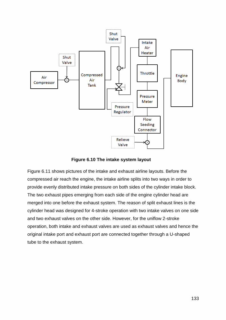
133
Figure 6.10 The intake system layout
Figure 6.11 shows pictures of the intake and exhaust airline layouts. Before the
compressed air reach the engine, the intake airline splits into two ways in order to
provide evenly distributed intake pressure on both sides of the cylinder intake block.
The two exhaust pipes emerging from each side of the engine cylinder head are
merged into one before the exhaust system. The reason of split exhaust lines is the
cylinder head was designed for 4-stroke operation with two intake valves on one side
and two exhaust valves on the other side. However, for the uniflow 2-stroke
operation, both intake and exhaust valves are used as exhaust valves and hence the
original intake port and exhaust port are connected together through a U-shaped
tube to the exhaust system.
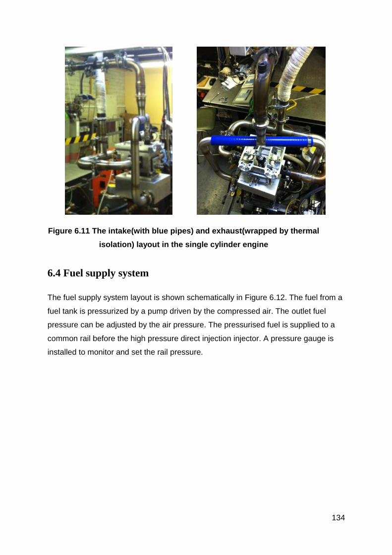
134
Figure 6.11 The intake(with blue pipes) and exhaust(wrapped by thermal
isolation) layout in the single cylinder engine
6.4 Fuel supply system
The fuel supply system layout is shown schematically in Figure 6.12. The fuel from a
fuel tank is pressurized by a pump driven by the compressed air. The outlet fuel
pressure can be adjusted by the air pressure. The pressurised fuel is supplied to a
common rail before the high pressure direct injection injector. A pressure gauge is
installed to monitor and set the rail pressure.

135
Figure 6.12 Fuel supply system layout
Figure 6.13 shows a picture of the fuel tank, fuel pump and the fuel rail. The pump is
an air driven plunger pump (Powerstar 4 S64P4S64). The fuel output pressure is
determined by the ratio between the area of the air drive piston, the area of the liquid
drive piston and the applied driving air pressure. The relationship of the driven air
pressure and the outlet fuel pressure, and the corresponding flow rate is shown in
Figure 6.14.
The compressed air used to drive the pump is delivered by the pressurized airline in
the laboratory; the air pressure can go up to 8bar. The pressure of air was then
regulated down to the required value to control the fuel outlet pressure.

136
Figure 6.13 Fuel tank, air driven pump and fuel rail
Figure 6.14 Air Pump performance curve
Fuel Tank Air Driven Pump
Fuel Rail

137
The fuel injector for experimental test engine is a Mahle gasoline piezo injector NGM
00084766. The injector was designed for high fuel injection pressure. The injection
fuel spray is a 94º cone shape continuous surface.
6.5 Spark ignition system and Timing Unit
A separate spark ignition control system is built and used to control the spark ignition
as shown in Figure 6.15.
Figure 6.15 Spark ignition control system
The function of Lucas ‘Dial-A-Time’ unit is to pick up a reference signal and
generates a spark ignition trigger with adjustable time offset and signal width. To
achieve the function, Lucas ‘Dial-A-Time’ unit requires a reference signal and a clock
signal to set the timing and width of the spark ignition, which are provided by a shaft
encoder mounted onto the end of the crank shaft. This encoder generates a TTL
signal for each revolution of the crankshaft as well as crank angle based clock
signals of a resolution of 1ºCA.
The clock signal from the shaft encoder allows the spark timing to be set in crank
angles rather than absolute time. The reference signal is generated by an “AND”
gate logical unit which picks up signals from the crank shaft encoder and a signal
generated by a cam sensor on the exhaust valve cam shaft pulley wheel. This
original spark ignition system was designed for the 4-stroke operation which takes
two revolutions per engine cycle. For the 2-stroke operation, the cam shaft signal is

138
set to high at all time so that a spark ignition signal is generated at each engine
revolution by the Lucas ‘Dial-A-Time’ unit to initiate the spark ignition.
Figure 6.16 Timing sequence for fuel injection and image acquisition
As shown in Figure 6.16, in addition to the spark timing, the reference signal
generated at 80ºBTDC is also used via a multi-channel signal generator to initiate
the fuel injection and the image acquisition process, as to be detailed in the next
chapter.
6.6 In-cylinder pressure and heat release analysis
The in-cylinder pressure measurement is obtained by a Kistler type 6055B80 piezo-
electric pressure transducer, which is capable of measuring pressure up to 250bar
with a sensitivity of 19.4 pC/bar and uncertainty of ± 0.1%. The transducer output
signal is then send to a charge amplifier Kistler type model 568 via a high impedance
cable. The charge amplifier converts the charge signal from the transducer into a
voltage signal. This voltage signal was calibrated using a dead weight test bed to
assign the output voltage to correct pressure. This analogue pressure signal is sent
to a National Instrument board type NI USB-6251 Data Acquisition (DAQ) card, the
DAQ card is a multifunction data acquisition card with 16-bits resolution and a
sampling rate of 1.25 MS/s. The DAQ card then converts the analogue signal into
digital signal using the shaft encoder output as the clock with a resolution of 1ºCA

139
and can be displayed in real time. The heat release results can then be calculated
using a bespoke LabView programme based on the first law thermodynamics.
6.7 Summary
This chapter describes the design and implementation of the modifications to a
single cylinder optical engine in order to achieve uniflow 2-stroke engine operations
and allow in-cylinder flow and mixture measurements by laser techniques. By
configuring the piston location relative to the intake ports and camshaft phase to the
crankshaft, the engine breathing was set to intake ports opening duration from
120ºATDC to 240ºATDC, and the exhaust valve opening duration was set to
80ºATDC to 240ºATDC. The intake air boosting system and high pressure fuel
supply system was also described. For the experiments, the intake pressure can go
up to 3bar absolute pressure and the fuel pressure can go up to 250bar.
140
Chapter 7 In-Cylinder Flow Measurements with
PIV
7.1 Introduction
This chapter presents the investigation of in-cylinder flow structure by means of the
Particle Image Velocimetry (PIV) method. PIV is a non-intrusive optical technique for
two-dimensional velocity measurements based on the displacement of particle
images over a known time interval, the displacement is calculated as follows,
[E-7.1]
– Velocity vector
– Element displacement
– Time interval
In order to obtain particle images, a laser light sheet is used to illuminate the
particles in the flow and the scattered light is captured by a camera, as shown in
Figure 7.1. In order to calculate the flow velocity vectors, the laser unit and the
camera are synchronized so that two images with a known time delay can be
recorded onto two separate frames by employing the so-called frame straddling
technique as shown in Figure 7.2. The pair of images is divided into a matrix of
interrogation areas (IA) of ( pixels, in which the cross-correlation analysis is
performed to determine the average particle displacement vector and then the
velocity vector.

141
Figure 7.1 Typical PIV experimental setup
Figure 7.2 Straddling technique

142
7.2 Experimental setup of PIV
7.2.1 Flow seeding
The seeding particles should be non-toxic, non-corrosive, non-abrasive, non-volatile
and chemically inert, as well as being small enough to faithfully follow the flow
changes [72]. The seeding material used in this experiment is vegetable oil. The
seeding generator is a 10F03 seeding generator supplied by Dantec Dynamics.
Figure 7.3 shows the diagram of the 10F03 seeding generator.
Figure 7.3 Flow seeding generator
Atomization of the seeding particles takes place according to Bernoulli’s principle as
shown below,
[E-7.2]
Seeding particle material
Blowing channel regulator Atomiser
regulator Release valve
Seeding flow outlet
Compressed air
Air capillary Seeding fluid
capillary

143
– Pressure
– Density
– Velocity
– Gravity
– The elevation of the point above a reference plane
The compressed air passes into the atomiser via the atomiser regulator to the air
tube. The high flow velocity flow field at the exit of the compressed air tube causes a
pressure drop near the tip of the other tube partially immersed in the liquid according
to Bernoulli’s principle. This vacuum sucks out the liquid which is dispersed into
small droplets by the high speed air flow. The liquid droplets are then blown to the
outlet of the seeding generator by the air flow in the chamber. The seeding generator
10F03 can continuously supply seeding flow with an average droplet size of Sauter
Mean Diameter (SMD) 2μm to 5μm up to a pressure of 3bar.
7.2.2 PIV Laser
The Nd: YAG laser is the most commonly used laser for PIV measurements due to
its high pulse energy. To achieve PIV measurements, two laser pulses within a short
time interval are required. Two methods with Nd: YAG laser can satisfy the
requirement, a single cavity Nd: YAG laser with double pulse option or a twin-
oscillator, twin-amplifier frequency doubled Nd: YAG laser [73]. The illumination of
PIV with the single cavity Nd: YAG laser is achieved by gating a single flash lamp
discharge from the single cavity laser to provide two laser shots. This method limits
the time interval between the two laser pulses to a range of 20μs to 200μs, which will
greatly reduce the laser light intensity and laser pulse width. In this study, a twin-
oscillator, twin-amplifier frequency doubled Nd: YAG laser has been used, which
allows an infinite and independent control over the time interval, width and intensity
of the laser pulses.
The laser unit used for the PIV experiments is NANO L 135-15 PIV laser by Liton
Lasers. The laser unit is powered by the LPU 450 power station configured to drive 2
laser units with a 450W combined throughput. The laser head consists of two
1064μm laser units, half wave plates, mixing and steering polarisers and a harmonic

144
generator. The laser head supplies 532μm laser beams with up to 136mJ laser pulse
energy under a 160μs optimised Q-switch delay.
7.2.2 Camera and Optics
The images of flow with seeding particles are captured with a Dantec Dynamic
FLOWSENSE 4M Camera system with a CCD camera of 2048x2048 pixels, which
has a minimum inter-frame time of 200ns.
The lens used for the PIV test is an UV-Nikkor 105 mm lens. A 532nm narrow band
filter is also used to remove background light. The configuration of the lens is shown
in Table 7.1.
Table 7.1 UV-Nikkor 105mm lens configuration
Focal Length 105mm
Aperture f/32 to f/4
Reproduction Ratio 1:10 to 1:2
Lens Elements 6
Lens Groups 6
Maximum Angle of View 23º12’
7.2.3 PIV test setup
The PIV test experimental setup is shown in Figure 7.4. The Nd: YAG laser sheet
was guided to the cylinder window ring by a high power long mirror arm for 532nm
light wavelength, as shown in Figure 7.5. A 45º mirror directs the scattering light of
in-cylinder flow seeding particles to the camera, and the camera set at the horizontal
level was used to capture the in-cylinder images. Both the laser unit and camera was
triggered by a set of signals synchronised with the reference signal.

145
Figure 7.4 PIV test layout
Figure 7.5 Laser lining setup
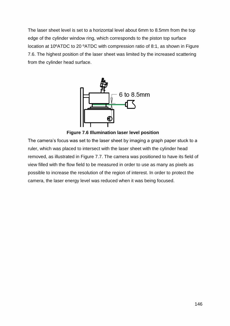
146
The laser sheet level is set to a horizontal level about 6mm to 8.5mm from the top
edge of the cylinder window ring, which corresponds to the piston top surface
location at 10ºATDC to 20 ºATDC with compression ratio of 8:1, as shown in Figure
7.6. The highest position of the laser sheet was limited by the increased scattering
from the cylinder head surface.
Figure 7.6 Illumination laser level position
The camera’s focus was set to the laser sheet by imaging a graph paper stuck to a
ruler, which was placed to intersect with the laser sheet with the cylinder head
removed, as illustrated in Figure 7.7. The camera was positioned to have its field of
view filled with the flow field to be measured in order to use as many as pixels as
possible to increase the resolution of the region of interest. In order to protect the
camera, the laser energy level was reduced when it was being focused.

147
Figure 7.7 Adjusting camera focus with an assisting subject
In the current experiments, the best particle images were obtained with a low f-
number of 4 due to its shorter depth of view. It was found that the maximum laser
output of 136mJ was required to produce sufficient scattering light from the small oil
droplets. The time interval of two laser pulses and camera actions were adjusted
from 30μs to 200μs, depending on the measurement time, in order to minimize the
dropout rate of the velocity vectors.
7.3 Evaluation of the particle displacement vector
The calculation of particle displacement vector evaluation was carried out by Dantec
Dynamics software Dynamicstudio based on the cross-correlation method. With this
method, the images recording the flow seeding particle position information is
divided into a number of square interrogation areas. The velocity vector evaluation of
each interrogation area is calculated by cross-correlation method. For this PIV
experimental setup, a 32x32 pixels interrogation area was used combined with the
Gaussian algorithm, which corresponds to a spatial resolution of 1.8mm x 1.8mm.
The cross-correlation method can be explained as follows. There is a random
distribution of particles in each interrogation area, which corresponds to certain
pattern of N particles in the flow,

148
[E-7.3]
with
– The state of the particle ensemble at a given time t
– The position vector of the particle i at time t, in the interrogation area of the
laser sheet
For following analysis, capital letters refer to the coordinates in the image plane, so
that
Lower case letters are used to represent the coordinates in the object plane, so that
and
where M is the magnification factor of the imaging system.
The image intensity of a single exposure can therefore be written as [69]
[E-7.4]
Where is the point spread function of the imaging lens and describes the
impulse response of the imaging lens and represents the system transfer
function, giving the light energy of the image of an individual particle inside the
interrogation area IV and its conversion into an electric signal.
The next stage is to calculate the cross correlation of the interrogation areas for the
pair of exposures. At this point it is advantageous to offset the two interrogation
areas according to an estimated mean particle displacement [75]. This increases the
fraction of matched to unmatched particle images, thereby increasing the signal to
noise ratio at the correlation peak. The cross correlation function for each pair of
interrogation areas is then calculated and the peak displacement vector is
determined, which corresponds to the particle image displacement vector.

149
Assuming there is a constant displacement of all particles inside the interrogation
area within the region of interest, the particle positions recorded in the second frame
are given by:
[E-7.5]
– The constant displacement of particles in the interrogation area
The corresponding particle image displacement can be given by:
[E-7.6]
The intensity distribution of the interrogation area for the second exposure can
therefore be described as:
[E-7.7]
For the first capture, it can be described as:
[E-7.8]
The cross-correlation function of the two interrogation areas can then be written as:
[E-7.9]
where s is the separation plane in the correlation plane.
By distinguishing the terms, which represent the correlation of different particle
images and therefore randomly distributed noise in the correlation plane, and the
terms which contain the desired displacement data, following expression can be
derived:
or

150
[E-7.10]
which can be divided into three parts:
[E-7.11]
where the first two terms and contribute to the background noise in the
correlation plane, both resulting from the terms. represents the
component of the cross correlation function that corresponds to the correlation of
images of particles obtained from the first exposure with images of identical particles
obtained from the second exposure ( terms) i.e.
[E-7.12]
Hence, this displacement correlation reached its peak at s=D, which means that the
average particle image displacement vector D can be determined from the maximum
of the displacement correlation distribution in the correlation plane, with the sign of D
defining the direction of flow.
Although correlation can be calculated by Equation 7.9, the most efficient way of
calculating correlation in practice is carried out by fast Fourier transform (FFT)
algorithms, which is used in this case and processed by the Dynamicstudio analyse
software.
The correlation theorem states that the cross-correlation of two functions is
equivalent to a complex conjugate multiplication of their Fourier transforms:
[E-7.13]
where and are the Fourier transforms of the functions I and I' respectively. The
cross correlation function can therefore be calculated by computing two two-
dimensional FFT's on equal sized samples of the image, followed by a complex-
conjugate multiplication of the resulting Fourier coefficients.

151
7.4 Results of PIV test
The PIV measurements were carried out at 90ºCA BTDC, 60ºCA BTDC and 30ºCA
BTDC, which corresponds to 30ºCA, 60ºCA and 90ºCA after the intake ports were
closed by the piston. Each measurement was repeated at three different intake
pressures of 1.2bar, 1.4bar and 1.6bar. The engine speed was set to 600rpm, which
equals to 1200 rpm engine speed for 4-stroke operation. PIV images of velocity
vectors were recorded for each measurement point and then ensemble-averaged.
7.4.1 In-cylinder flow structure on the horizontal plane @ 600rpm engine speed
a) Boost pressure 1.2bar b) Boost pressure 1.4bar
C) Boost pressure 1.6bar
Figure 7.8 Averaged flow structure @90ºCABTDC

152
As shown in Figure 7.8, swirl flows are detected in the measurement plane.
However, the swirl flow structure is relatively unstable, high flow speed occurs along
the area adjacent to either top side or bottom side of the image, corresponding to the
regions next to the two opposite intake ports banks. More than one vortex centres
are present at higher boost pressures of 1.4bar and 1.6bar.This suggests that while
intake pressure increases, the intake flow kinetic energy is higher, this higher flow
kinetic energy creates small vortex in the swirl flow structure, especially at the stage
right after the intake process.
a) Boost pressure 1.2bar b) Boost pressure 1.4bar
c) Boost pressure 1.6bar
Figure 7.9 Averaged flow structure @60ºCABTDC
Figure 7.9 shows the in-cylinder flow structure at 60ºCA BTDC. Compared with the
flow field at the earlier crank angle, a more dominant swirl flow structure can be
observed with one swirl flow centre as the other smaller vortices are merged into the

153
dominant one near the centre. In addition to the dominant swirl flow structure, there
are many areas of low velocities, such as the right side and top side of the image in
Figure 7.9 (a), both left and right side of the image in Figure 7.9 (b) and the right side
of the image shown in Figure 7.9 (c). In these areas, the vertical flow dominates the
air flow during the scavenging process, the CFD simulation results showed this
vertical flow structure as in Figure 7.10. As the piston moves up, the vertical flow
movements are enhanced with little change in the flow field in the horizontal plane.
Figure 7.10 CFD simulation results of in-cylinder flow structure on the
horizontal (top) and vertical plane (bottom) @60ºCABTDC
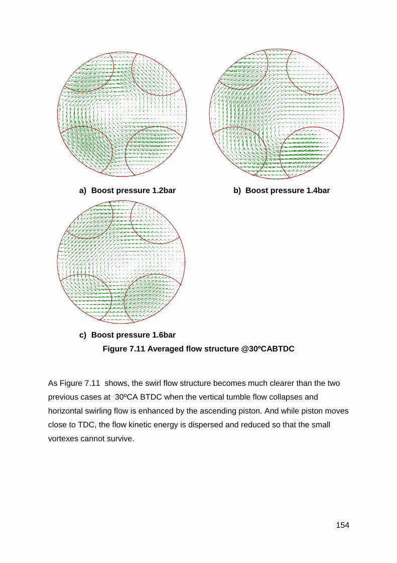
154
a) Boost pressure 1.2bar b) Boost pressure 1.4bar
c) Boost pressure 1.6bar
Figure 7.11 Averaged flow structure @30ºCABTDC
As Figure 7.11 shows, the swirl flow structure becomes much clearer than the two
previous cases at 30ºCA BTDC when the vertical tumble flow collapses and
horizontal swirling flow is enhanced by the ascending piston. And while piston moves
close to TDC, the flow kinetic energy is dispersed and reduced so that the small
vortexes cannot survive.

155
(a1) PIV results at 30ºCABTDC (a2) CFD results at 30ºCABTDC
(b1) PIV results at 60ºCABTDC (b2) CFD results at 60ºCABTDC
(c1) PIV results at 90ºCABTDC (c2) CFD results at 90ºCABTDC
Figure 7.12 Measured and flow fields with 1.2bar pressure

156
As shown in Figure 7.12, the CFD results are very similar to the PIV results at the
three crank angles in terms of both the global flow structures and their evolution
during the compression process.
Figure 7.13 shows the spatially averaged velocity values in the measurement plane.
Both CFD and PIV results show that higher boost pressure leads to higher in-
cylinder flow velocity and the average velocity decrease as the piston moves to TDC.
In general, the CFD results show higher velocities than the PIV measurements.
However, as the piston moves up towards TDC, the difference becomes smaller.

157
a) Boost pressure 1.2bar
b) Boost pressure 1.4bar
c) Boost pressure 1.6bar
Figure 7.13 Average velocity of the region of interest
0
2
4
6
8
10
12
14
16
18
30BTDC-1.2bar 60BTDC-1.2bar 90BTDC-1.2bar
Ve
loci
ty [
m/s
]
Experimental
CFD-ROI
0
5
10
15
20
25
30
35
40
30BTDC-1.4bar 60BTDC-1.4bar 90BTDC-1.4bar
Velo
cit
y [
m/s
] Experimental
CFD-ROI
0
10
20
30
40
50
60
70
80
90
30BTDC-1.6bar 60BTDC-1.6bar 90BTDC-1.6bar
Velo
cit
y [
m/s
]
Experimental
CFD-ROI

158
7.4.2 In-cylinder flow structure on the horizontal plane @ 900rpm engine speed
In order to investigate the effect of engine speed on in-cylinder flows , the engine
speed was increased to 900rpm, beyond which the timing belt drive may not be
sufficient robust.
a) Boost pressure 1.2bar b) Boost pressure 1.4bar
c) Boost pressure 1.6bar
Figure 7.14 Averaged flow structure @90ºCABTDC
Figure 7.14 shows the in-cylinder flow structure at 900rpm engine speed with 1.2bar,
1.4bar and 1.6bar boost pressures. Compared with the 600rpm, the swirl flow pattern
can be hardly observed because of the stronger upward flow with higher piston
speed. While the piston speed increases, the piston movement input extra kinetic

159
energy to the flow vertical movement, which interrupting the horizontal swirl flow
structure.
a) Boost pressure 1.2bar b) Boost pressure 1.4bar
c) Boost pressure 1.6bar
Figure 7.15 Averaged flow structure @60ºCABTDC
As the piston moves up to 60ºCA BTDC, as shown in Figure 7.15, the swirl flow
structure pattern begins to appear. However, because higher boost pressure delivers
higher flow kinetic energy, the swirl pattern is less clear at higher boost pressure for
the same reason as 600rpm engine speed

160
a) Boost pressure 1.2bar b) Boost pressure 1.4bar
c) Boost pressure 1.6bar
Figure 7.16 Averaged flow structure @30ºCABTDC
As shown in Figure 7.16, the piston moves to 30ºCA BTDC, the swirl flow structure is
much clearer than the cases at 90ºCA BTDC and 60ºCA BTDC, following a similar
trend to the results at 600rpm.

161
Figure 7.17 Average velocity across the region of interest on the horizontal
plane
Figure 7.18 Swirl ratio across the region of interest on the horizontal plane
Figure 7.17 shows the average velocity across the region of interest on the
horizontal plane. The results suggest that the increase in the engine speed from
600rpm to 900rpm has fairly small effect on the averaged horizontal flow, which is
dominated by the intake port orientation instead.
Figure 7.18 shows the swirl ratios of the flows in the measurement plane calculated
according to Equation 3.10. As the boost pressure becomes higher, the swirl ratio is
increased by stronger radial flow because of the swirl intake port design. When the
0
5
10
15
20
25
30
35
40
45
1.2Bar 1.4Bar 1.6Bar
Ve
loci
ty[m
/s]
30BTDC-600rpm
60BTDC-600rpm
90BTDC-600rpm
30BTDC-900rpm
60BTDC-900rpm
90BTDC-900rpm
0
2
4
6
8
10
12
1.2Bar 1.4Bar 1.6Bar
Swir
l Rat
io
30BTDC-600rpm
60BTDC-600rpm
90BTDC-600rpm
30BTDC-900rpm
60BTDC-900rpm
90BTDC-900rpm

162
engine speed is increased from 600rpm to 900rpm, the swirl ratios dropped because
of the enhanced vertical tumble flow and shorter time at the higher engine speed.
In conclusion, at early stage of the flow structure creating process, the swirl flow
structure is not stable and sensitive to the piston moving speed and intake boost
pressure. However, as the piston moves towards TDC, as the flow kinetic energy
disperses and reduces the small vortexes disappear and only the swirl flow structure
can be obtained.
7.5 Summary
This chapter has discussed the experimental setup of a PIV system and its
application to in-cylinder flow field measurements in the single cylinder 2-stroke
uniflow engine with optical access. The in-cylinder flow fields and their evolution
during the compression stroke were presented and the effects of intake pressure and
engine speed were investigated. In addition, the PIV results were compared with the
CFD calculations. It has been shown that strong swirl flows are formed just before
TDC in all the cases and their swirl ratios increase with boost pressure and drops
slightly at higher engine speeds.

163
Chapter 8 In-Cylinder Measurements of Fuel
Distribution and Flame Propagation in
the Uniflow 2-stroke Engine
8.1 Introduction
The fuel injection and distribution directly affect the air/fuel mixture quality and the
subsequent combustion and pollutant formation process. This chapter focuses on
the fuel distribution by the Planar Laser-Induced Fluorescence (PLIF) method and
flame propagation imaging in the experimental uniflow 2-stroke engine. The principle
of PLIF and the experimental setup are described. The experimental results of
engine fuel distribution and flame propagation are discussed.
8.2 Principle of the PLIF Technique
Planar Laser Induced Fluorescence (PLIF) is a very popular optical measuring
technique for the instantaneous measurement of whole-field concentration of a
species. The process of laser induced fluorescence is depicted in Figure 8.1. Upon
radiation by a laser beam, a molecule or atom is excited from its ground electronic
state to a higher energy level. This is followed by the loss of energy to an
intermediate energy state and then emission of photons to the ground electronic
state.

164
Figure 8.1 Energy level diagram of LIF
A two-energy level model is used for the LIF analysis. The rate equations for the
lower and upper energy levels are described as follows:
[E-8.1]
[E-8.2]
where
– Einstein coefficient for stimulated absorption
– Einstein coefficient for stimulated emission
– Einstein coefficient for spontaneous emission
– Laser spectral intensity
– Coefficient for collisional excitation energy
– Coefficient for collisional energy loss
– Coefficient for Photo ionization energy
– Coefficient for Predissociative energy

165
– Population of state 1 and 2
The collisional excitation energy coefficient can be omitted in most cases, most
excited states are not predissociative and the photo ionization coefficient can be
ignored also. Thus, the Equation 8.1 and 8.2 can be simplified as follows:
[E-8.3]
[E-8.4]
The upper energy level population can be negligible prior to the laser excitation, for
the initial condition, . In addition, the total population of molecules should
be conserved because no chemical reaction occurs. So,
[E-8.5]
where
– Total population of tracer atom prior to laser excitation
The solution of two-energy-level system is given by
[E-8.6]
[E-8.7]
For laser pulse longer than to , the system reaches its steady value, presented as
follows,
[E-8.8]
[E-8.9]
where
– The saturation intensity

166
Assuming the fluorescence is emitted onto a full sphere evenly, the total number of
photons captured by the image sensor from a collection volume is given by
[E-8.10]
where
– Transmission efficiency of the collection optics
– The collection solid angle
– The spectral fluence of the laser
– The sampling volume
8.3 PLIF experimental setup
The engine configuration for the experimental setup of the PLIF test is the same as
that used for the PIV tests described in Chapter 7. The major differences are the
laser, the transmitting optics and imaging system.
A Xenon Chloride (XeCl) Excimer laser with 308nm wavelength was used for the
PLIF measurement, the laser specifications are shown in Table 8.1.
Table 8.1 XeCl laser specifications
Type XeCl
Model COMPexPro 102
Max Output Power 4 W
Wavelength 308 nm
Pulse Energy 200 mJ
Pulse Length 20 ns
Pulse Repetition Rate Max 20 Hz
Beam Size (V×H) 24mm×10 mm
Beam Divergence (FWHM) 3 mrad Vertical
1 mrad Horizontal
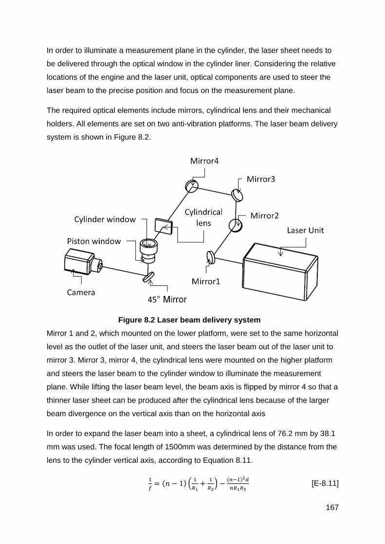
167
In order to illuminate a measurement plane in the cylinder, the laser sheet needs to
be delivered through the optical window in the cylinder liner. Considering the relative
locations of the engine and the laser unit, optical components are used to steer the
laser beam to the precise position and focus on the measurement plane.
The required optical elements include mirrors, cylindrical lens and their mechanical
holders. All elements are set on two anti-vibration platforms. The laser beam delivery
system is shown in Figure 8.2.
Figure 8.2 Laser beam delivery system
Mirror 1 and 2, which mounted on the lower platform, were set to the same horizontal
level as the outlet of the laser unit, and steers the laser beam out of the laser unit to
mirror 3. Mirror 3, mirror 4, the cylindrical lens were mounted on the higher platform
and steers the laser beam to the cylinder window to illuminate the measurement
plane. While lifting the laser beam level, the beam axis is flipped by mirror 4 so that a
thinner laser sheet can be produced after the cylindrical lens because of the larger
beam divergence on the vertical axis than on the horizontal axis
In order to expand the laser beam into a sheet, a cylindrical lens of 76.2 mm by 38.1
mm was used. The focal length of 1500mm was determined by the distance from the
lens to the cylinder vertical axis, according to Equation 8.11.
[E-8.11]

168
where
– Lens focal length
– The refractive index of the lens material
– The curvature radii on the two lens surfaces
– Required distance from lens to the subject to be focused on
The lens used in this case is anti-reflection coated by CVI Melles Griot BBAR4 248-
355 coating, which provides both a very low reflection of 0.5% over a broad UV
range from 248 nm to 355 nm and very high damage threshold. The resulting laser
sheet thickness was about 1mm.
The fluorescence images via the 45o mirror in the cylinder block were recorded by a
Princeton Instrument PI-MAX III intensified CCD camera with the Nikon 105mm UV
lens. A ST-133 controller with the Programmable Timing Generator (PTG) used to
control the camera timing. A PC with an interface card and Princeton Instrument
WinView/32 software was used to setup configurations and carry out data analysis.
3-pentanone was used as the fluorescence tracer for the PLIF measurements due to
its high fluorescence yield and its similar boiling point (102 °C) to the iso-octane
(99 °C) which was used due to its absence of deposit formation on the optical
window. In this study, a mixture of 90% of iso-octane and 10% of 3-pentanone was
used. The properties of iso-octane and 3-pentanone was as described in table 2.1.
8.4 Results of PLIF measurements
The PLIF measurement was carried out at 900rpm with all other engine operating
parameters kept the same as the PIV experiment in Chapter 7. The direct fuel
injection timing was set to 60ºCA BTDC. The injector used in this test was a Siemens
gasoline piezo injector (NGM 00084766) with a cone shaped spray structure.
8.4.1 Fuel Injection characteristics
Figure 8.3 shows the first appearance of fuel spray at 110μs after the start of the fuel
injection trigger sent to the injector. The injection duration was set to 200 μs. This

169
110μs delay corresponds to the electro mechanical lag of the injector needle opening,
which was found to be constant at different injection timings and durations.
Figure 8.3 First spray image at 110μs after injector trigger signal (200μs
duration)
As shown in Figure 8.4, the last image of fuel spray leaving the injector was found at
470μs after the start of the injection trigger. Taking into account of the injection
duration (200 μs) and the injector opening delay (110 μs), there was a delay of 160
μs for the injector needle to be fully seated after the end of the injection trigger. In
addition, it is noted that there is an area of strong fluorescence emission on the
injector side (right side of the image), indicating the occurrence of fuel spray
impingement on the piston.

170
Figure 8.4 The end of Injection image at 470μs after injector trigger signal
(200μs duration)
Figure 8.5 shows the fuel spray structure at 500μs after the start of injection trigger
(30 μs after the closure of the injector needle). At this stage, a second fuel spray
cloud was present around the injector although only one injection trigger was applied.
This could be a result of the bounce of the needle valve when it was closed due to
excessive force, which could be eliminated by optimising the injector drive signal.

171
Figure 8.5 In-cylinder image at 500μs after injector trigger signal (200μs
duration)
Figure 8.6 shows the fuel spray patterns at 600μs, 700μs, 1000μs and 2000μs after
the start of injection trigger. At 600μs the second fuel injection was finished. At
700μs, two fuel sprays mixed together and higher fuel concentration was present on
the far side to the injector, due to the pent roof combustion chamber shape and the
angle of injector. Because of its much higher velocity and momentum, the early fuel
spray development was hardly affected by the strong in-cylinder swirl flow.

172
600μs 700μs
1000μs 2000μs
Figure 8.6 In-cylinder images of the fuel distribution
8.4.2 Fuel distribution at 15°CA BTDC
For the fuel distribution study, PLIF images of different conditions were taken at
15ºCA BTDC when the spark ignition was to take place with the Start Of Injection
(SOI) timing set to 60ºCA BTDC. The boost pressure was set to 1.2bar, 1.4bar and
1.6bar. The fuel injection pressure was set to 100bar, 150bar and 200bar for each
intake boost pressure and the injection duration set at 200μs, 300μs and 400μs. For
each condition, twenty images were taken from consecutive engine cycles and the
same process was repeated 5 times, so that an ensemble averaged image of 100
frames was obtained and analysed. One background image was taken without fuel
injection prior to the PLIF fuel images and used to remove the ambient light from the
reflection and other light sources.

173
For the post-processing of the fuel distribution data, a mean light intensity of all
pixels in the region of interest (Imean) was calculated. The region of interest was a
round shape area with 50mm diameter, which is the visible in-cylinder area. This
value can be used for the comparison of the in-cylinder fuel quantity. Then the
deviation of the light intensity at each pixel from the mean light intensity was
calculated as the CoV of each ensemble averaged frame (CoVf), this value can be
used to indicate the homogeneity of fuel distributions. For all images taken at the
same engine operating condition, an average value of the mean light intensity of
each frame was calculated, and then the deviation of the mean light intensity to the
ensemble average value was used to calculate the CoV of the images taken at same
engine condition (CoVcyc). This value was used to present the cyclic variation. The
calculations are shown as follows,
[E-8.12]
[E-8.13]
[E-8.14]
[E-8.15]
where
– The pixel number in the region of interest
– The frame number of each image batch taken at same condition
– The light intensity of each pixel
– The mean light intensity of all pixels in the region of interest of each frame
– The mean light intensity of all frames taken at same condition

174
a) Injection duration 200μs b) Injection duration 300μs
c) Injection duration 400μs
Figure 8.7 In-cylinder images of the fuel distribution with 1.2bar boost
pressure and 100bar fuel injection pressure
Figure 8.7 shows the in-cylinder fuel distribution images taken under 1.2bar intake
boost pressure and 100bar fuel injection pressure, the fuel injection trigger pulse
width was set to 200μs, 300μs and 400μs.
As expected, the PLIF image is characterized with stronger light intensity and larger
areas of the higher intensity as more fuel is injected. In addition, the fuel distribution
appears more homogenous with more fuel injected.
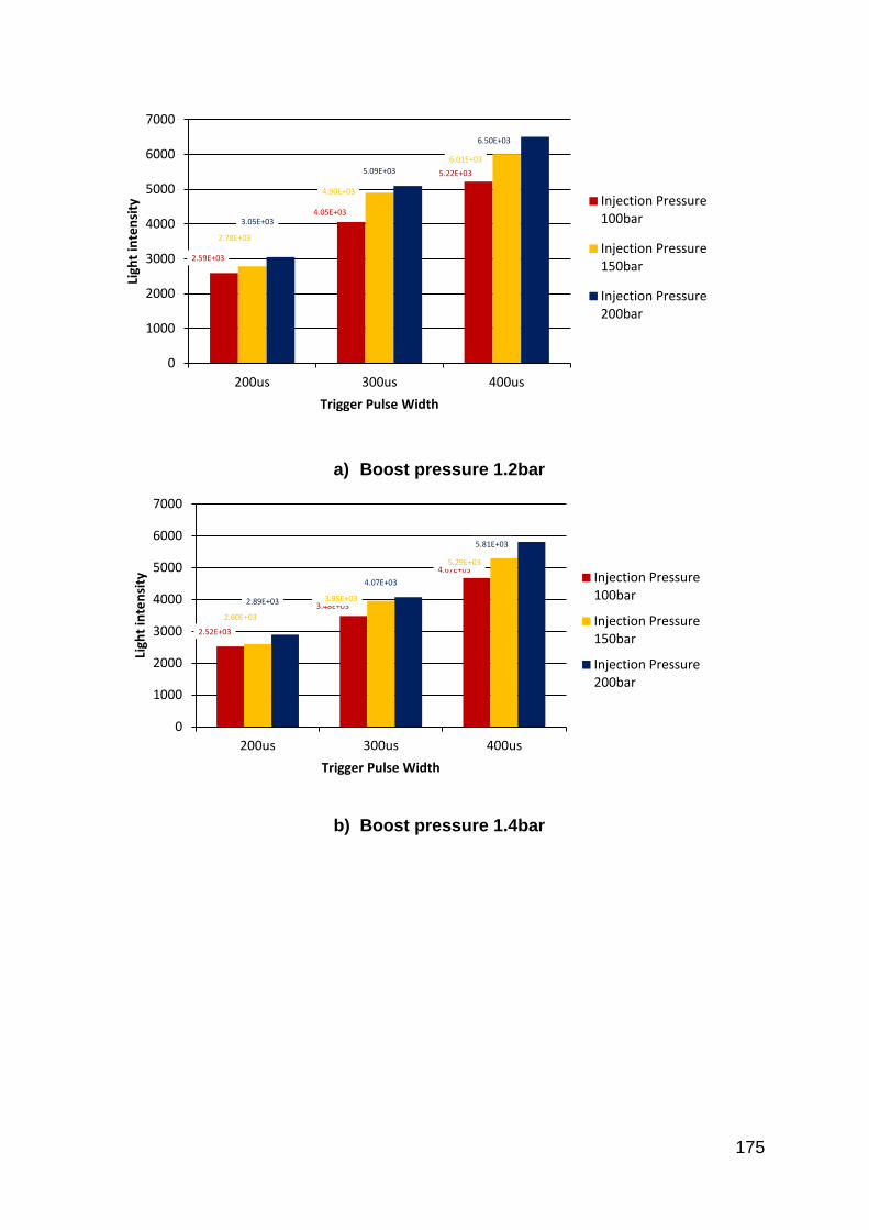
175
a) Boost pressure 1.2bar
b) Boost pressure 1.4bar
2.59E+03
4.05E+03
5.22E+03
2.78E+03
4.90E+03
6.01E+03
3.05E+03
5.09E+03
6.50E+03
0
1000
2000
3000
4000
5000
6000
7000
200us 300us 400us
Ligh
t in
ten
sity
Trigger Pulse Width
Injection Pressure 100bar
Injection Pressure 150bar
Injection Pressure 200bar
2.52E+03
3.48E+03
4.67E+03
2.60E+03
3.95E+03
5.29E+03
2.89E+03
4.07E+03
5.81E+03
0
1000
2000
3000
4000
5000
6000
7000
200us 300us 400us
Ligh
t in
ten
sity
Trigger Pulse Width
Injection Pressure 100bar
Injection Pressure 150bar
Injection Pressure 200bar
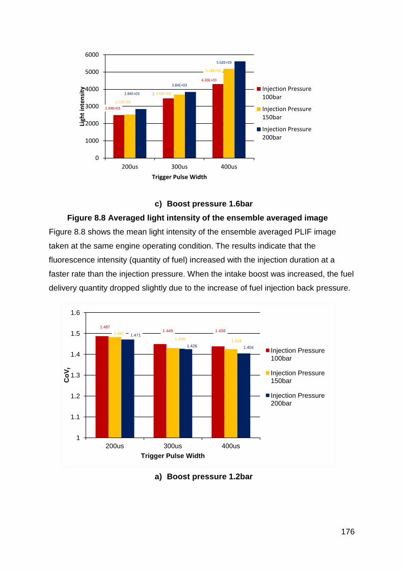
176
c) Boost pressure 1.6bar
Figure 8.8 Averaged light intensity of the ensemble averaged image
Figure 8.8 shows the mean light intensity of the ensemble averaged PLIF image
taken at the same engine operating condition. The results indicate that the
fluorescence intensity (quantity of fuel) increased with the injection duration at a
faster rate than the injection pressure. When the intake boost was increased, the fuel
delivery quantity dropped slightly due to the increase of fuel injection back pressure.
a) Boost pressure 1.2bar
2.49E+03
3.46E+03
4.30E+03
2.53E+03
3.68E+03
5.18E+03
2.84E+03
3.84E+03
5.62E+03
0
1000
2000
3000
4000
5000
6000
200us 300us 400us
Ligh
t in
ten
sity
Trigger Pulse Width
Injection Pressure 100bar
Injection Pressure 150bar
Injection Pressure 200bar
1.487 1.449 1.438
1.483
1.430 1.424
1.471
1.426 1.404
1
1.1
1.2
1.3
1.4
1.5
1.6
200us 300us 400us
Co
Vf
Trigger Pulse Width
Injection Pressure 100bar
Injection Pressure 150bar
Injection Pressure 200bar

177
b) Boost pressure 1.4bar
c) Boost pressure 1.6bar
Figure 8.9 CoVf of the light intensity in the ensemble averaged image
Figure 8.9 shows the spatial variation of light intensity, CoVf, in each ensemble
averaged image. With either longer fuel injection duration or higher fuel injection
pressure, the spatial variation of fluorescence light intensity became smaller,
indicating a more uniform fuel distribution. The intake boost pressure barely showed
any effect on fuel distribution uniformity. Related research work has suggested that
the introduction of swirl creates a velocity drop near the cylinder centre in the radial
profiles of axial velocity, and as the swirl strength is increased, the drop gets wider
and the centreline velocity decreases [76]. The reduction in flow is undesirable as it
can result in not only a poorly scavenged central region but also a poor air/fuel
1.485 1.451 1.434 1.485
1.439
1.417
1.475
1.429 1.401
1
1.1
1.2
1.3
1.4
1.5
1.6
200us 300us 400us
Co
Vf
Trigger Pulse Width
Injection Pressure 100bar
Injection Pressure 150bar
Injection Pressure 200bar
1.486 1.451 1.437
1.475 1.440
1.410
1.466
1.432 1.412
1
1.1
1.2
1.3
1.4
1.5
1.6
200us 300us 400us
Co
Vf
Trigger Pulse Width
Injection Pressure 100bar
Injection Pressure 150bar
Injection Pressure 200bar

178
mixture area. With the swirl scale generated by the intake ports orientation and the
intake boost pressure used, the results indicate that the fuel distribution was
dominated by the fuel injection process due to much higher spray kinetic energy than
the swirl flow.
a) Boost pressure 1.2bar
b) Boost pressure 1.4bar
0.158
0.132
0.111
0.129
0.099
0.095
0.148
0.105
0.065
0
0.05
0.1
0.15
0.2
0.25
0.3
200us 300us 400us
Co
Vc
yc
Trigger Pulse Width
Injection Pressure 100bar
Injection Pressure 150bar
Injection Pressure 200bar
0.175
0.076
0.130
0.133 0.134
0.072
0.121
0.102
0.078
0
0.05
0.1
0.15
0.2
0.25
0.3
200us 300us 400us
Co
Vc
yc
Trigger Pulse Width
Injection Pressure 100bar
Injection Pressure 150bar
Injection Pressure 200bar

179
c) Boost pressure 1.6bar
Figure 8.10 CoVcyc of image batch at same condition
As shown in Figure 8.10, the cyclic variation of the averaged light intensity, CoVcyc
was low in all cases, an indication of excellent repeatability of the DI. In most of the
cases, higher fuel delivery quantity resulted in the lowest cyclic variation. Figure 8.11
shows individual images taken with 200μs fuel injection duration, 100bar fuel
injection pressure and 1.2bar boost pressure. Although variation in terms of fuel
distribution can be observed, in terms of overall light intensity, the variation is very
small.
0.116
0.140 0.149
0.140
0.121
0.119
0.136
0.084
0.093
0
0.05
0.1
0.15
0.2
0.25
0.3
200us 300us 400us
Co
Vc
yc
Trigger Pulse Width
Injection Pressure 100bar
Injection Pressure 150bar
Injection Pressure 200bar

180
Figure 8.11 Fuel distribution - 200μs fuel injection trigger, 100bar fuel
injection pressure and 1.2bar boost pressure
8.4.3 Fuel distribution at 15°CA BTDC and SOI 120°CA BTDC
Further PLIF measurements at 15ºCA BTDC were carried out with an earlier fuel
injection timing of 120ºCA BTDC at the same engine operating condition. As shown
in Figure 8.12, for all engine operating conditions, the advanced fuel injection timing
reduced the CoVf of the fuel distribution and produced a more homogeneous charge.
This suggests that for this particular case, advanced fuel injection timing is preferred
considering the in-cylinder charge homogeneity.

181
100bar fuel injection pressure and SOI
@ 60ºCA BTDC
100bar fuel injection pressure and
SOI @ 120ºCA BTDC
150bar fuel injection pressure and SOI
@ 60ºCA BTDC
150bar fuel injection pressure and
SOI @ 120ºCA BTDC
200bar fuel injection pressure and SOI
@ 60ºCA BTDC
200bar fuel injection pressure and
SOI @ 120ºCA BTDC
Figure 8.12 CoVf of the fuel distribution
1.3
1.35
1.4
1.45
1.5
1.55
1.6
200us 300us 400us
Co
Vf
Fuel Injection Trigger Pulse
1.2bar
1.4bar
1.6bar
1.3
1.35
1.4
1.45
1.5
1.55
1.6
200us 300us 400us
Co
Vf
Fuel Injection Trigger Pulse
1.2bar
1.4bar
1.6bar
1.3
1.35
1.4
1.45
1.5
1.55
1.6
200us 300us 400us
Co
Vf
Fuel Injection Trigger Pulse
1.2bar
1.4bar
1.6bar
1.3
1.35
1.4
1.45
1.5
1.55
1.6
200us 300us 400us
Co
Vf
Fuel Injection Trigger Pulse
1.2bar
1.4bar
1.6bar
1.3
1.35
1.4
1.45
1.5
1.55
1.6
200us 300us 400us
Co
Vf
Fuel Injection Trigger Pulse
1.2bar
1.4bar
1.6bar
1.3
1.35
1.4
1.45
1.5
1.55
1.6
200us 300us 400us
Co
Vf
Fuel Injection Trigger Pulse
1.2bar
1.4bar
1.6bar

182
For the cyclic variation, although the injection timing was advanced, the improvement
of cyclic variation was not realized. As discussed for the cases under 600rpm engine
speed, the cyclic variation is actually very low, furthermore, the in-cylinder flow
structure creating process was random to a certain extent which would affect the
cyclic variation results. Advancing the fuel injection timing in this case would not
improve the cyclic variation further.
The results of in-cylinder fuel distribution measurements suggests that while
considering the in-cylinder mixture quality, richer mixture is preferred, in this case,
the lambda value of 1 is preferred. However, no direct results indicating the
relationship between lean mixture and the combustion performance. Furthermore, for
SI combustion, due to the narrow time window between the end of engine breathing
process and the suitable combustion timing, the fuel injection timing is suggested to
be as early as possible after all ports and valves are closed.
8.5 Combustion Studies
In order to obtain images of in-cylinder combustion, the window ring in cylinder liner
was replaced by a metal ring with the same dimensions. The engine speed was
600rpm and spark timing at 15ºCA BTDC. The fuel injection timing was set to 60ºCA
BTDC. The boost pressure was 1.2bar and air/fuel ratio was 14.7. The intake port
opening duration is from 120ºCA ATDC to 240ºCA ATDC and exhaust valve opening
duration is 90ºCA ATDC to 240ºCA ATDC. The direct chemiluminescence of flame
was recorded without laser illumination.
The engine in-cylinder pressure and heat release rate data are shown in Figure 8.13
and 8.14. The heat release calculation was shown below,
[E-8.16]
where
– Heat release rate
– Specific heat ratio

183
– In-cylinder pressure
– In-cylinder volume
The engine IMEP was 2bar. The CA10, CA50 and CA90 were at 9ºCA BTDC, 2ºCA
ATDC and 31ºCA ATDC, respectively. The heat release result illustrated a relatively
long and low heat release process at the late stage of the combustion. This heat
release process can also be observed in the images taken at late flame propagation
stage, a small flame core lasted about 5 ºCA to 10ºCA after the rapid burning
process. This is probably because of the effect of the in-cylinder swirl flow structure,
the flow structure kept mixing the unburned fuel and other in-cylinder components,
diluting the unburned air/fuel mixture, thus the combustion speed was reduced.
Figure 8.13 In-cylinder pressure curve
0
5
10
15
20
25
30
35
40
-180 -90 0 90 180
Pre
ssu
re[b
ar]
Crank Angle [°CA]

184
Figure 8.14 Heat release curve
Two image acquisition systems were used for the flame propagation study on the
uniflow 2-stroke engine. A NAC Memrecam fx 6000 high speed video camera
coupled with a DRS Hadland Model ILS3-11 intensifier was used to record the high
speed frame sequence continuously with 512x384 pixel resolution at 6000fps.
Higher resolution snapshot images from different cycles were obtained by the
Princeton ICCD camera.
15ºCA BTDC 9ºCA BTDC)
-10
0
10
20
30
40
50
60
70
80
-30 0 30 60
He
at r
ele
ase
rat
e [
J]
Crank Angle [°CA]

185
6ºCA BTDC 3ºCA ATDC
15ºCA ATDC 18ºCA ATDC
Figure 8.15 Flame Propagation images sequence
Figure 8.15 shows the high speed sequence of images of combustion taken by the
high speed video camera. After the ignition, the flame kernel was forced to the
bottom side of the image. Both the flame centre and the flame front moved in the
clockwise direction due to the effect of in-cylinder swirl flow. As it approached the
cylinder wall, the flame front was quenched around TDC. The flame region seen at
15ºCA ATDC and afterwards was most likely caused by the combustion of locally
fuel rich mixture and after-burn of CO to CO2 in the burned gas region.

186
15ºCA BTDC 10ºCA BTDC (CA10)
5ºCA BTDC TDC (CA50)
5ºCA ATDC 10ºCA ATDC

187
15ºCA ATDC 20ºCA BTDC
Figure 8.16 Flame Propagation images
Figure 8.16 shows the higher resolution individual images from different cycles taken
by the ICCD camera PI-MAX III. Although all images were taken from different cycles,
the results still suggest that the flame was blown toward one side of the cylinder wall
and then shrunk back to the flame core around the centre of the combustion
chamber. The higher temperature core and after-burn near the spark plug are
particularly visible.
With the in-cylinder flow structure and strength organized by current engine
configuration, the flow is not too strong to breach the flow propagation sequence, but
also not too weak that will be broken by the expansion of the combustion. The flame
propagation was dominated by the combustion expansion at early stage and
dominated by the in-cylinder swirl flow when the kinetic energy of the combustion
explosion getting lower. This feature could be helpful for improving the combustion
efficiency especially at the late stage of the combustion and could be helpful for
reducing engine emissions.
8.6 Summary
This chapter explained the engine configuration and experimental facilities for PLIF
measurements on fuel distribution study and the flame propagation study in the
uniflow 2-stroke engine.
For the fuel distribution study, various intake boost pressures, fuel injection
pressures, injection durations and fuel injection timings were used. The results were

188
compared in terms of the fuel delivery quantity indicated by the fluorescence
intensity; the fuel distribution uniformity presented by the CoVf and the cyclic
variation measured by CoVcyc.
For the flame propagation study, two camera systems has been used in order to take
continuous frame sequence and high resolution images taken cycle by cycle. The
results from two systems were consistent.

189
Chapter 9 Conclusions and Recommendations
for Future Work
9.1 Introduction
Research has been carried out on the feasibility and potential of a boosted uniflow 2-
stroke direct injection gasoline engine as a highly downsized powerplant for
automotive applications. Both numerical calculations and engine experiments were
carried out in the study.
3D CFD calculation was used for in-cylinder flow structure and fuel distribution
studies. In addition, the results of the 3D CFD calculations were used to set up the
initial and boundary conditions for the 1D engine simulation, which significantly
reduced the complexity and time spent in the engine simulation and predictions. The
geometry of the boosted uniflow engine was then optimised for maximum
performance.
Following the simulation study, a uniflow 2-stroke single cylinder engine was
commissioned with a newly designed intake engine block. The block features uniflow
intake ports and incorporates optical access for in-cylinder measurements. The PIV
technique was used for in-cylinder flow structure measurements and the PLIF
technique for the in-cylinder fuel distribution measurements. Stable combustion was
achieved and the combustion process was studied by means of high speed imaging.
9.2 Design of intake ports
Different intake port designs were analysed using CFD in order to evaluate their
effects on in-cylinder flow characteristics. The main findings of the 3D CFD
calculations are as follows:
(i) As the axis inclination angle is changed from 30º to 90º with an increment of
15º, the delivery ratio increased due to enlarged effective area of the intake
ports. Because of the air short circuiting effect, the trapping efficiency falls as
the axis inclination angle increases. The charging and scavenging

190
performance of 60º and 75º axis inclination angle are slightly less than those
of the 90º axis inclination angle ports. In light of the negative effect of air short
circuiting of larger angles, 60º axis inclination angle was chosen in the
subsequent analysis.
(ii) For a given engine bore diameter and fixed value of the port width ratio, intake
ports can be arranged with wider port width and less number of ports or
narrower port width and more number of ports. The calculations has shown
that with the same swirl orientation angle and port width ratio, air mass flow
rate through intake ports is independent of the number of intake ports when
the port width ratio is kept constant. For a given swirl orientation angle, the
swirl ratio decreases slightly as the number of ports is reduced. That is, a
higher swirl ratio can be obtained with a larger number of narrower ports due
to higher flow velocity and more organised swirl flow.
(iii) When the swirl orientation angle is increased from 43º to 51º, the delivery
ratio falls gradually from 2.4 to 1.9, which requires a reduced port width ratio.
In addition, a larger swirl orientation angle produces a greater swirl ratio. The
best scavenging performance is obtained with a swirl orientation angle of 20°.
When the swirl orientation angle is less than 20°, the scavenging performance
and the trapping efficiency decrease because of the air short circuiting effect,
although the delivery ratio increases. When the swirl orientation angle
becomes greater than 20°, the scavenging performance also declines
because of the reduction in the delivery ratio. Therefore, the 60° axis
inclination angle and 20° swirl orientation angle has been adopted in the
uniflow 2-stroke engine design.
9.3 In-cylinder fuel distribution
The Discrete Phase Model is used to simulate the direct fuel injection process of an
outward open piezo DI gasoline injector with a 90º cone spray angle. The injected
fuel is treated as particles and droplet breakup calculation is included to model the
atomisation process. The results of the CFD calculations can be summarised as
follows:
(i) The fuel evaporation rate increases during the high pressure fuel injection
process and then slows down after the end of injection. Faster fuel

191
evaporation takes place at retarded injection timings due to higher charge
temperature. The main cause for the less total fuel vapour from the early
injection cases is the liquid fuel impingement because of the in-cylinder swirl
flow and lower charge density during the earlier injection.
(ii) Split injections were found to improve the fuel atomisation and mixture
formation. Because of the reduced momentum of each injection of shorter
duration, the split injection reduces the liquid impingement of early injection.
In addition, it is shown that the total fuel evaporation is improved as the
percentage of the first injection is reduced from 50% to 20%.
9.4 Uniflow engine geometry and scavenging timings
The uniflow 2-stroke engine design has been analysed by the 1D engine model with
calibrated Frictional Mean Effective Pressures (FMEP). The effect of bore and
stroke ratio on the engine performance was studied to determine the appropriate
bore and stroke of the 2-stroke engine. The impact of timings of the intake ports and
exhaust valves on engine performance was investigated. The main conclusions
include:
(i) The bore to stroke ratio for maximum engine performance is 1.13. In order to
accommodate the vehicle packaging, the stroke was fixed to 67mm.
Therefore, for the targeted 0.3 litre displacement volume per cylinder, a bore
of 76mm and stroke of 67mm were chosen
(ii) The intake port/exhaust valve timing optimisation has been carried out for
maximum performance. The intake port opening time is set to 120ºATDC, and
closure at 240ºATDC. The exhaust valve opening duration was set to
80ºATDC to 240ºATDC.
9.5 The boosted uniflow 2-stroke powertrain and its application to
a vehicle
The full load performance of the boosted uniflow 2-stroke engine dictates the number
of cylinders of such engines, which can ultimately help in selection of a suitable

192
boosting system according to its compressed air flow rate. In turn, the potential
benefits from engine downsizing and downspeeding will depend on the performance
of the boosted uniflow 2-stroke engine. The 1D engine simulation has been used to
assess the maximum torque and power which can be obtained from different
configurations of turbocharger and supercharger with the peak cylinder pressure
below 120bar. A vehicle driving simulation program was developed and applied to
analyse the fuel economy benefits over the NEDC. The main conclusions are as
follows:
(i) Among all the boost system configurations with various modes of
supercharger and turbocharger considered, the turbocharger shows the best
efficiency from a thermodynamic point of view. The low efficiency of the
supercharger is mainly due to the mechanical losses especially at low load.
(ii) Both the 3-cylinder 0.9 litre and the 2-cylinder 0.6 litre uniflow 2-stroke engine
are capable of matching the performance of the NA 1.6 litre 4-stroke engine
output with an optimised turbocharger.
(iii) With the same transmission ratio, the 3-cylinder 0.9 litre 2-strok engine
showed 8.6% increase in fuel consumption and the 2-cylinder 0.6 litre 2-
stroke engine improved the fuel economy by 8.2%. However, with 33.3%
downspeeding, the fuel economy can be improved by 12.6% by the 3-cylinder
engine and 18.1% respectively by the 2-cylinder engine, respectively. With
44.4% downspeeding strategy, the fuel economy went up to 18.3% and
23.6%.
9.6 Single cylinder uniflow 2-stroke engine and its in-cylinder
flow and fuel distributions
A single cylinder DI gasoline engine was converted to operate as an uniflow 2-stroke
engine by incorporating a new intake block, modified cylinder liner, a new timing belt
and crank sprocket, as well as customised intake and exhaust systems. The intake
block was designed with swirl intake ports based on the CFD calculations and
provided the optical access for the in-cylinder flow and fuel measurements. The
single cylinder engine was operated successfully up to 900rpm.

193
The in-cylinder flow measurements by PIV showed similar trend with the CFD
calculation. It was found that the swirl flow structure was less well defined at the end
of the intake process. The swirl flow structure became more apparent and the swirl
ratio was significantly enhanced at the end of the compression stroke due to the
piston movement and conservation of momentum.
During the in-cylinder fuel injection measurements, a delay between the injection
electrical drive signal and the start of injection was noted and it was measured as
110μs. A similar delay was also detected between the electrical drive signal and the
closure of the injector at the end of injection process. When the quantity of fuel
injected was small, the in-cylinder fuel distribution exhibited high cycle to cycle
variations. As the fuel injection was increased, the in-cylinder fuel distribution
became more uniformly distributed and showed less cyclic variations.
The uniflow 2-stroke engine was fired successfully by setting the intake port opening
duration to 120ºATDC and exhaust valves opening from 80º to 240ºATDC. Both high
resolution single shot images and crank angle resolved high speed flame
propagation images were recorded and analysed. Following its formation around the
spark plug, the flame was found to move towards one side of the combustion
chamber due to the in-cylinder swirling flow. The after-burn of locally fuel rich
mixtures was found after the flame front was extinguished.
9.7 Recommendations for future work
9.7.1 Engine simulations
In the current research, the 3D CFD simulation was used to model the effect of
intake port design and was able to show the general flow structure in the cylinder as
measured via the PIV technique. In order to use the 3D CFD to guide the design and
optimisation of the direct injection uniflow 2-stroke engine, further evaluation and
calibration of the fuel injection and spray models will be required. In addition, the
combustion model needs to be developed to predict the heat release process and
engine performance. Both spark ignition flame propagation and autoignition models
should be included in the combustion modelling so that the autoignition combustion
at part-load operation can be analysed as a function of engine parameters.

194
9.7.2 In-cylinder flow and fuel distribution measurements
The intake block in the single cylinder uniflow 2-stroke engine has the flexibility of
varying the intake port orientation. Due to the time constraint, only one intake port
design was implemented. It is recommended that additional experiments can be
carried out with different intake port designs in order to optimise the in-cylinder flow
and scavenging process. In addition to the in-cylinder flow and fuel distribution on a
horizontal plane, the PIV and PLIF techniques can be used to obtain the flow and
fuel distributions in a vertical plane through the optical liner. Although the in-cylinder
flame propagation investigation has been carried out, the test was only in initial state.
Further experimental tests and analysis work would be very helpful on understanding
the combustion characteristic of a uniflow 2-stroke engine.
9.7.3 Engine thermal and emission performance
Although fired engine operation was realised in the single cylinder uniflow 2-stroke
engine, it was difficult to carry out systematic thermodynamic engine experiments. In
order to evaluate the full potential of the uniflow 2-stroke direct injection gasoline
engine, it would be desirable to design and build such an engine that has the
capability to operate at speeds up to 3500rpm and withstand cylinder pressure up to
120bar. The engine should be equipped with variable cam timing devices on the
exhaust valves so that the scavenging process can be adjusted according to the
speed and load. The combustion system should include centrally mounted injector
and spark plug for optimum mixture formation. In addition, variable boost pressure
and exhaust back pressure should be provided to simulate the interactions between
the engine and a turbocharger.

195
References
[1] I. C. O. C. TRANSPORTATION, “EU CO2 EMISSION STANDARDS FOR
PASSENGER CARS AND LIGHT-COMMERCIAL VEHICLES,” January 2014.
[2] “New Car CO2 Report 2013,” The 12th report, 14 March 2013.
[3] F. Zhao, M.-C. Lai and D. Harrington (1999), “Automotive spark-ignited direct-
injection gasoline engines,” Energy and Combustion Science, vol. 25, p. 437–
562, 1999.
[4] T. Kume, Y. lwamoto, K. lida, M. Murakami, K. Akishino and H. Ando(1996),
“Combustion Control Technologies for Direct Injection SI Engine,” SAE
International, 960600.
[5] J. Harada, T. Tomita, H. Mizuno, Z. Mashiki and Y. Ito (1997), “Development of
Direct Injection Gasoline Engine,” SAE International, 970540.
[6] M. Kano, K. Saito, M. Basaki, S. Matsushita and T. Gohno (1998), “Analysis of
Mixture Formation of Direct Injection Gasoline Engine,” SAE Technical Paper,
980157.
[7] H. Zhao, J. Li, T. Ma and N. Ladommatos (2002), “Performance and Analysis of
a 4-Stroke Multi-Cylinder Gasoline Engine with CAI Combustion,” SAE
International, 2002-01-0420.
[8] L. Cao, H. Zhao, X. Jiang and N. Kalian (2005), “Numerical Study of Effects of
Fuel Injection Timings on CAI/HCCI Combustion in a Four-Stroke GDI Engine,”
SAE International, 2005-01-0144.
[9] A. Oakley, H. Zhao and N. Ladommatos (2001), “Experimental Studies on
Controlled Auto-ignition (CAI) Combustion of Gasoline in a 4-Stroke Engine,”
SAE International, 2001-01-1030.

196
[10] M. Christensen, B. Johansson, P. Amnéus and F. Mauss (1998), “Supercharged
Homogeneous Charge Compression Ignition,” SAE International, 980787.
[11] N. Ito, T. Ohta, R. Kono, S. Arikawa and T. Matsumoto (2007), “Development of
a 4-Cylinder Gasoline Engine with a Variable Flow Turbo-charger,” SAE
International, 2007-01-0263.
[12] D. Han, S.-K. Han, B.-H. Han and W.-T. Kim (2007), “Development of 2.0L
Turbocharged DISI Engine for Downsizing Application,” SAE International, 2007-
01-0259.
[13] T. Noyori, T. Ohira, T. Nakamura and Y. Akamatsu (2003), “Development of a
660cc Turbo-Charged Spark-Ignition Direct-Injection Engine,” SAE International
and Society of Automotive Engineers of Japan, Inc, 2003-32-0013 / 20034313.
[14] S. Keppeler, H. Schulte and H. J. Ecker (1998), “The Technical Ramifications of
Downsizing HSDI Diesel Technology to the 300 cc Displacement Class,” SAE
International, 981916.
[15] H. J. Ecker, M. Schwaderlapp and D. K. Gill (2000), “Downsizing of Diesel
Engines: 3-Cylinder / 4-Cylinder,” SAE International, 2000-01-0990.
[16] J. Turner, A. Popplewell, R. Patel, T. Johnson, N. Darnton, S. Richardson, S.
Bredda, R. Tudor, C. Bithell, R. Jackson, S. Remmert, R. Cracknell, J.
Fernandes, A. Lewis, S. Akehurst, C. Brace, C. Copeland, R. Martinez-Botas, A.
Romagnoli and A. Burluka (2014), “Ultra Boost for Economy: Extending the
Limits of Extreme Engine Downsizing,” SAE International, 2014-01-1185.
[17] T. Lake, J. Stokes, R. Murphy, R. Osborne and A. Schamel (2004),
“Turbocharging Concepts for Downsized DI Gasoline Engines,” SAE
international, 2004-01-0036.
[18] W. P. Attard, S. Konidaris, E. Toulson and H. C. Watson (2007), “The Feasibility
of Downsizing a 1.25 Liter Normally Aspirated Engine to a 0.43 Liter Highly
Turbocharged Engine,” SAE International, 2007-24-0083.

197
[19] M. Thirouard and P. Pacaud (2010), “Increasing Power Density in HSDI Engines
as an Approach for Engine Downsizing,” SAE International, 2010-01-1472.
[20] W. Attard, H. C. Watson, S. Konidaris and M. A. Khan (2006), “Comparing the
Performance and Limitations of a Downsized Formula SAE Engine in Normally
Aspirated, Supercharged and Turbocharged Modes,” SAE International, 2006-
32-0072.
[21] N. Fraser, H. Blaxill, G. Lumsden and M. Bassett (2009), “Challenges for
Increased Efficiency through Gasoline Engine Downsizing,” SAE International,
2009-01-1053.
[22] G. P. Blair (1990), “The basic design of two-stroke engines,” no. ISBN 1-56091-
008-9, 1990.
[23] “Daihasu press release, 58th Frankfurt Motor show.,” 14th September, 1999.
[24] R. Knoll (1998), “AVL Two-Stroke Diesel Engine,” SAE Technical Paper,
981038.
[25] J. Abthoff, F. Duvinage, T. Hardt, M. Krämer and M. Paule (1998), “The 2-Stroke
DI-Diesel Engine with Common Rail Injection for Passenger Car Application,”
SAE Paper, 981032.
[26] Y. Moriyoshi, K. Kikuchi, K. Morikawa and H. Takimoto (2001), “Numerical
Analysis of Mixture Preparation in a Reverse Uniflow-Type Two-Stroke Gasoline
DI Engine,” SAE Paper, 2001-01-1815/4235.
[27] E. C. O. Pereira, E. F. A. Rodrigues and J. J. G. Martins (1997), “Design of a
Fuel Efficient Uniflow Two Stroke Semi-Direct Injection Engine,” SAE Paper,
970367.
[28] E. Mattarelli, C. A. Rinaldini, G. Cantore and P. Baldini (2012), “2-Stroke
Externally Scavenged Engines for Range Extender Applications,” SAE
International, 2012-01-1022.

198
[29] Y. Li, H. Zhao, Z. Peng and N. Ladommatos (2001), “Analysis of Tumble and
Swirl Motions in a Four-Valve SI Engine,” SAE International, 2001-01-3555.
[30] M. Lorenz and K. Prescher (1990), “Cycle Resolved LDV Measurements on a
Fired SI-Engine at High Data Rates Using a Conventional Modular LDV-
System,” SAE International, 900054.
[31] A. E. Catania, C. Dongiovanni, A. Mittica, G. Molina and E. Spessa (1995), “A
New Test Bench for HWA Fluid-Dynamic Characterization of a Two-Valved In-
Piston-Bowl Production Engine,” SAE International, 952467.
[32] F. E. Corcione and G. Valentino (1990), “Turbulence Length Scale
Measurements by Two-Probe-Volume LDA Technique in a Diesel Engine,” SAE
Technical Paper Series, 902080.
[33] M. Auriemma, F. E. Corcione, R. Macchioni, G. Seccia and G. Valentino (1996),
“LDV Measurements of Integral Length Scales in an IC Engine,” SAE
TECHNICAL PAPER SERIES, 961161.
[34] S.-C. Yoo, K. Lee, M. Novak, H. Schock and P. Keller (1995), “3-D LDV
Measurement of In-Cylinder Air Flow in a 3.5L Four-Valve SI Engine,” SAE
TECHNICAL PAPER SERIES, 950648.
[35] T. Obokata, T. Hashimoto, S.-i. Gojuki, T. Karasawa, S. Shiga and T.
Kurabayashi (1992), “LDA Characterization of Gas Flow in a Combustion
Chamber of a Four-Stroke S.I. Engine,” SAE International, 920519.
[36] D. W. LEE (1938), “A STUDY OF AIR FLOW IN AN ENGINE CYLINDER,”
LANGLEY llLIEMORIAL AERONAUTICAL LABORATORY, NTATIONAL
ADVISORY COMMITEE FOR AERONAUTICS, LANGLEY FIELD, REPORT No.
653 September 16, 1938.
[37] M. Rönnbäck and W. X. Le (1991), “Study of Induction Tumble by Particle
tracking Velocimetry in a 4-Valve Engine,” SAE International, 912376.
[38] H.-J. Neußer, L. Spiegel and J. Ganser (1995), “Particle Tracking Velocimetry -

199
A Powerful Tool to Shape the In-Cylinder Flow of Modern Multi-Valve Engine
Concepts,” SAE TECHNICAL PAPER SERIES, 950102.
[39] L. Fan, R. D. Reitz and N. Trigui (1999), “Intake Flow Simulation and
Comparison with PTV Measurements,” SAE TECHNICAL PAPER SERIES,
1999-01-0176.
[40] G. Valentino, L. Allocca and L. Marchitto (2011), “PIV Investigation of High Swirl
Flow on Spray Structure and its Effect on Emissions in a Diesel-Like
Environment,” SAE International, 2011-01-1286.
[41] M. Ekenberg, R. Reinmann, E. Olofsson, B. Gillet and B. Johansson (2001),
“The Influence of a Late In-Cylinder Air Injection on In-Cylinder Flow Measured
with Particle Image Velocimetry (PIV),” SAE International, 2001-01-3492.
[42] W. Zeng, M. Sjöberg and D. Reuss (2014), “Using PIV Measurements to
Determine the Role of the In-Cylinder Flow Field for Stratified DISI Engine
Combustion,” SAE International, 2014-01-1237.
[43] B. Khaligh (1990), “Intake-Generated Swirl and Tumble Motions in a 4-Valve
Engine with Various Intake Configurations- Flow Visualization and Particle
Tracking Velocimetry,” SAE International, 900059.
[44] D. H. Shack and W. C. Reynolds (1991), “Application of Particle Tracking
Velocimetry to the Cyclic Variability of the Pre-Combustion Flow Field in a
Motored Axisymmetric Engine,” SAE TECHNICAL PAPER SERIES, 910475.
[45] W. Church and P. V. Farrell (1998), “Effects of Intake Port Geometry on Large
Scale In-Cylinder Flows,” SAE International, 980484.
[46] D. L. Reuss, T.-W. Kuo, B. Khalighi, D. Haworth and M. Rosalik (1995), “Particle
Image Velocimetry Measurements in a High-Swirl Engine Used for Evaluation of
Computational Fluid Dynamics Calculations,” SAE International, 952381.
[47] D. L. Reuss (2000), “Cyclic Variability of Large-Scale Turbulent Structures in
Directed and Undirected IC Engine Flows,” SAE International, 2000-01-0246.
200
[48] S. Haider, T. Schnipper, A. Obeidat, K. E. Meyer, V. L. Okulov, S. Mayer and J.
H. Walther (2013), “PIV study of the effect of piston position on the in-cylinder
swirling flow during the scavenging process in large two-stroke marine diesel
engines,” Journal of Marine Science and Technology, vol. 18, no. 1, pp. 133-
143 , 2013.
[49] C. Arcoumanis, H. G. Green and J. H. Whitelaw (1985), “Velocity and
concentration measurements in a model diesel engine,” Experiments in Fluids,
vol. 3, pp. 270-276, 1985.
[50] T. Ksdota, F.-Q. Zhao and K. Miyosh (1990), “Rayleigh Scattering
Measurements of Transient Fuel Vapor Concentration in a Motored Spark
Ignition Engine,” SAE Technical Paper, 900481.
[51] C. Espey, J. E. Dec, T. A. Litzinger and D. A. Santavicca (1994), “Quantitative 2-
D Fuel Vapor Concentration Imaging in a Firing D.I. Diesel Engine Using Planar
Laser-Induced Rayleigh Scattering,” SAE Technical Paper, 940682.
[52] P. Miles and M. Dilligan (1996), “Quantitative In-Cylinder Fluid Composition
Measurements Using Broadband Spontaneous Raman Scattering,” SAE
Technical Paper, 960828.
[53] C. Schulz and V. Sick (2005), “Tracer-LIF diagnostics: quantitative measurement
of fuel concentration, temperature and fuel/air ratio in practical combustion
systems,” Energy and Combustion Science, vol. 31, p. 75–121, 2005.
[54] W. Hwang, J. E. Dec and M. Sjöberg (2007), “Fuel Stratification for Low-Load
HCCI Combustion: Performance & Fuel-PLIF Measurements,” SAE
International, 2007-01-4130.
[55] S. Shen and I. Nagata (1995), “Prediction of excess enthalpies of ketone-alkane
systems from infinite dilution activity coefficients,” Thermochimica Acta, vol. 258,
pp. 19-31, 1995.
[56] X. Wang, Z. Zhan, X. Yu, T. Hu, Y. Qiao, Y. Zhu and S. Jiang (2014),
“Experimental Study on Injector Spray Pattern Optimization for a Turbocharged

201
GDI Engine Combustion System,” SAE International, 2014-01-1439.
[57] V. S. Movva (2004), “SIMULATION OF FLUID FLOW IN INTERNAL
COMBUSTION ENGINES USING WAVE ACTION SIMULATION,” MASTER OF
SCIENCE. Thesis, 2004. Texas Tech University.
[58] S. A. Orszag and I. Staroselsky (2000), “CFD: Progress and problems,”
Computer Physics Communications, 127 (2000) 165–171.
[59] P. Sagaut (1998), Large Eddy Simulation for Incompressible Flows, An
Introduction, Springer, 1998.
[60] G. Alfonsi (2009), “Reynolds-Averaged Navier–Stokes Equations for Turbulence
Modeling,” Transactions of the ASME, vol. 62, no. 040802-20, JULY 2009.
[61] U. G. Riegler and M. Bargende (2002), “Direct Coupled 1D/3D-CFD-
Computation (GT-Power/Star-CD) of the Flow in the Switch-Over Intake System
of an 8-Cylinder SI Engine with External Exhaust Gas Recirculation,” SAE
International, 2002-01-0901.
[62] C. Forte, E. Corti, G. M. Bianchi, S. Falfari and S. Fantoni (2014), “A RANS CFD
3D Methodology for the Evaluation of the Effects of Cycle By Cycle Variation on
Knock Tendency of a High Performance Spark Ignition Engine,” SAE Technical
Paper, 2014-01-1223.
[63] L. Cornolti, A. Onorati, T. Cerri, G. Montenegro and F. Piscaglia (2013), “1D
simulation of a turbocharged Diesel engine with comparison of short and long
EGR route solutions,” Elsevier Applied Energy, 111 (2013) 1–15.
[64] “ANSYS FLUENT 12.0/12.1 Documentation,” 2009-01-29 .
[65] J. B. Heywood (1988), Internal Combustion Engine Fundamentals, 1988.
[66] K. Jaffri, H. G. Hascher, M. Novak, K. Lee, H. Schock, M. Bonne and P. Keller
(1997), “Tumble and Swirl Quantification within a Motored Four-Valve SI Engine
Cylinder Based on 3-D LDV Measurements,” SAE International, 970792.

202
[67] G. D’Errico, A. Onorati and S. Ellgas (2008), “1D thermo-fluid dynamic modelling
of an S.I. single-cylinder H2 engine with cryogenic port injection,” Elsevier
International Association for Hydrogen Energy, 3 3 ( 2 0 0 8 ) 5 8 2 9 – 5 8 4 1.
[68] “WAVE help system 8.3,” 2010.
[69] S. K. Chen and P. F. Flynn (1965), “Development of Single Cylinder
Compression Ignition Research Engine,” SAE Paper, 650733.
[70] Z. J. Sroka (2012), “Some aspects of thermal load and operating indexes after
downsizing for internal combustion engine,” J Therm Anal Calorim, vol. 110, p.
51–58, 2012.
[71] A. Melling (1997), “Tracer particles and seeding for particle image velocimetry,”
Meas. Sci. Technol., vol. 8, p. 1406–1416, 1997.
[72] H. Zhao (2012), Laser Diagnostics and Optical Measurement Techniques, ISBN
978-0-7680-5782-9, 2012.
[73] R. J. Adrian (1991), “PARTICLE-IMAGING TECHNIQUES FOR
EXPERIMENTAL FLUID MECHANICS,” Annual Reviews. Fluid Mech., vol. 23,
pp. 261-304, 1991.
[74] J. Westerweel (1997), D. Dabiri and M. Gharib, “The effect of a discrete window
offset on the accuracy of cross-correlation analysis of digital PIV recordings,”
Experiments in Fluids, vol. 23, pp. 20-28, 1997.
[75] K. M. Ingvorsen, K. E. Meyer, J. H. Walther and S. Mayer (2013), “Turbulent
swirling flow in a model of a uniflow-scavenged two-stroke engine,” Experiment
Fluids, no. 54:1494, 2013.
[76] C. J. Rutland (2011), “Large-eddy simulations for internal combustion engines -
a review,” International Journal of Engine Research, p. 12: 421, 2011.

203
Appendix
Figure. A1 Engine block extension modification
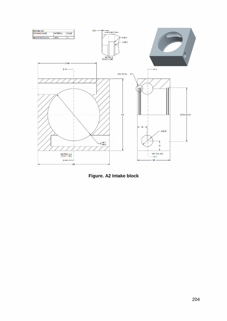
204
Figure. A2 Intake block

205
Figure. A3 Port block
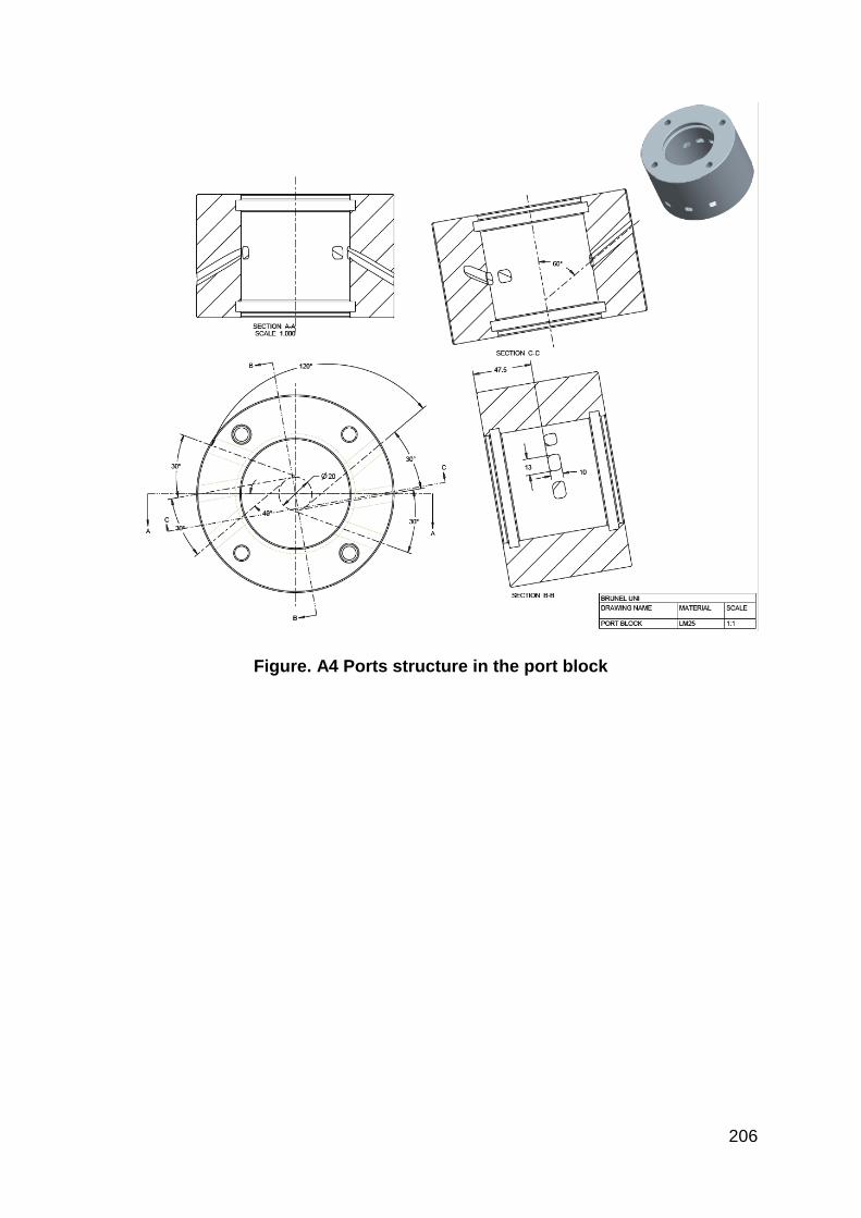
206
Figure. A4 Ports structure in the port block

207
Figure. A5 Piston extension

208
Figure. A6 Piston head