numerical and experimental study of parametric rolling of

Numerical and Experimental Study of

Parametric Rolling of a Container Ship in Waves

Emre UzunogluCentre of Marine Technology

Technical University of LisbonInstituto Superior [email protected]

Abstract

The paper deals with the validation and calibrationof a theoretical method and its numerical solution toforesee the susceptibility of a vessel to the occurrenceof parametric rolling. A frequency domain and a timedomain code are used in conjunction for numericalprocedures. This study aims to validate both codes bycomparing them to the experimental results of scaledmodel testing of a C11 type container vessel. In or-der to validate the frequency domain code which usestrip theory, results of the forced oscillations tests arecompared. Then, the time domain numerical resultsare checked against parametric rolling tests. As theforced oscillation tests include the evaluation of theheeled vessel as well, the results reveal the change inhydrodynamic coefficients in heave and pitch due tothe heeling of the vessel. Furthermore, a third pro-gram was developed in scope of this study in orderto facilitate the usage of the two programs mentionedabove and to speed up the process considerably.

1 Introduction

Intact stability has been a concern for all floatingstructures that have ever been built. The first treatythat deals with this subject was passed in 1914, andit has been updated constantly. Even with the up-dated version, the regulations have generally beenoverlooked. Parametric rolling in head seas, specifi-cally came into attention around the fifties. However,in October 1998, a C11 type container ship has lost1/3 of its deck containers and damaged another 1/3in a severe storm attracting renewed attention to thephenomenon [1].

To address this issue, over the past nine years,Instituto Superior Tecnico has been working on thedevelopment of a numerical model for the calculation

of the movements of vessels in regular and irregularwaves [2]. However to fully validate the code, it wasnecessary to conduct experiments and compare themto the results of the code. With this aim, a series oftests were carried out on a C11 type container ship inthe El Pardo towing tank in Madrid.

For the estimation of parametric rolling, the avail-ability of an adequate motion calculation routine ca-pable of predicting the time domain large ampli-tude responses under resonant conditions is impor-tant [3]. In that aspect, this study aims to validatethe frequency domain and time domain codes thatare used in conjunction to estimate large amplitudeship motions. The frequency domain code suppliesthe time domain code with the hydrodynamic coef-ficients (heave and pitch added mass and damping)and the exciting forces. The obtained hydrodynamiccoefficients are evaluated in here by comparison to theforced oscillation tests of the heeled and upright ves-sel. While it has been shown that even up to 5 degreesof heel the change in hydrodynamic coefficients maybe considerable [4], this study reveals results up to10 degrees of heel. Furthermore, the the parametricrolling experiments are compared to the simulationresults.

2 The computer codes

There are two codes that are used to simulate para-metric rolling in this work. The frequency domaincode calculates the hydrodynamic coefficients, andthe exciting forces. The time domain code uses thisinput as initial values and simulates the motions ofthe vessel using six degrees of freedom. While therestoring forces and exciting forces are calculated dy-namically depending on the wave profile at instant,the added mass and damping are considered to bestatic. This interaction between the programs require

1

Table 1: Main particulars of the vessel

Item Value

Length btw. perp. (Lpp) 262.00 mDepth (D) 24.40 mBreadth (BDWL) 40.00 mDisplacement (∇DWL) 76056 tBlock coefficient (CB) 0.66Draught (TDWL) 12.34 mTransverse metacentric height (GMT ) 1.973 mNatural roll period (T44) 22.78 sMax. speed (U) 20 knots

constant interaction and file conversation. In orderto fully automatize the process a third program wasdeveloped in this work. This third application car-ries out the necessary file conversation and presentsa user interface eliminating the need to have knowl-edge of the structures used. Furthermore it adds addi-tional functionality by estimating roll damping usingMiller’s method or energy methods. As uninterruptedrange operations (e.g. calculate a range of 0 - 10 knotsin 1 knot steps) are made possible by the developmentof this interface, data can also be obtained for polarplots.

3 Validation of the Hydrody-namic Coefficients Prediction

The experiments in CEHIPAR included a wide rangeof tests in order to allow a full understanding of thebehaviour of the vessel. However, two parts of testswere analysed in particular. The first part of the testsare the forced oscillation tests and the second is theparametric rolling tests. The vessel that has beenselected is a C11 type container vessel with the mainparticulars presented in table 1.

In order to assess the hydrodynamic coefficientsof heave and pitch, forced oscillation tests were con-ducted on the vessel. These tests consist of forcingthe model to execute harmonic heave and pitch mo-tions at a predefined frequency and amplitude. Forthe assessment of speed effects, 7.97 and 0 knots wereselected. All tests were repeated for six different fre-quencies of motion. Moreover, three different am-plitudes for each motion were tested to evaluate thenon-linearities involved. The summaries of heave andpitch forced oscillation experiments are presented intables 2 and 3 respectively. Each table represents atotal of 52 tests.

For the analysis of the experiments a program

Table 2: Forced oscillation tests (Heave)

Variable Values

speed (kts) 0 / 7.97heel (deg) 0 / 5 / 10amplitudes (m) 0.4 / 0.8 / 1.2oscillation periods (s) 9.2 / 11.2 / 12.9 /

15.8 / 17.1 / 18.3

Table 3: Forced oscillation tests (Pitch)

Variable Values

speed (kts) 0 / 7.97heel (deg) 0 / 5 / 10amplitudes (deg) 1 / 2 / 3oscillation periods (s) 9.2 / 11.2 / 12.9 /

15.8 / 17.1 / 18.3

called “Fota” (forced oscillation tests analysis) wasdeveloped in this work. The program trims downthe time series of motions and forces to strip themoff the transient phases. Then, trough curve fitting,it obtains the sinusoidal signals that are to be anal-ysed. Once the motions and forces are obtained, theforces are reduced to hydrodynamic forces only bythe removal of restoring and inertial forces. Then theremaining hydrodynamic forces relate to the addedmass and damping in their respective modes utilizingthe following formulae:

Aij =FD.cos(ϕ)

A.ω2o

(1)

Bij = −FD.sin(ϕ)

A.ωo(2)

where FD stands for the hydrodynamic force, ϕstands for the phase angle between the force and themotion. While A is the amplitude of motion, ω rep-resents the oscillation frequency.

3.1 Comparison of Forced Oscillationand Strip Theory Results

In the figures 1(a) to 6(d), complete results for heaveand pitch motions are presented. The experimentalresults are represented by points where each shaperepresents a different amplitude of motion. The nu-merical calculations are represented by a line. The Xaxis shows the periods of oscillation and the Y axisshows the actual value of the hydrodynamic coeffi-cient.

2

It is worthy of notice that there are two codes usedin this comparison. While the first code calculatesthe upright numerical values the second code carriesout calculations for the heeled vessel. As giving zerodegrees of heel (i.e. defining the vessel as upright) tothe second code would result in the same values as thefirst code, only one line defines the numerical results.

The heave motion results are presented in figures1(a) to 3(d). When the heave added mass is exam-ined, it is seen to be in closer agreement with the the-ory at higher frequencies. Non-linear effects are vis-ible as the results from different amplitudes of teststend to “spread-out” especially in lower frequencies(for a clear example, see figure 1(c)). If the effect ofspeed is considered, speeding up to 7.97 knots doesseem to introduce higher deviations from the exper-imental results, especially in higher frequencies. Ingeneral, it is possible to state that the values areslightly underestimated apart from the 10◦ (figures3(a) and 3(c)), where the correlation is very good.This finding may be interesting to assess the perfor-mance of strip theory in heeled sections.

The damping in heave motion, B33, is estimatedwell by the numerical code when there is no speed, yetthere is a tendency to underestimate it with speed.The non-linearities are highly visible also for heavedamping. Regardless of speed, the values are under-estimated for the 10 degrees of heel (figures 3(b) and3(d)). Generally the curvature of the damping re-sults follow the average of the experimental results. Inhere, the damping results are not extremely affectedby the oscillation period, going beyond the generalstrip theory assumption of high frequency motion.

The pitch added inertia and damping results arepresented in figures 4(a) to 6(d). When the addedinertia is paid close attention to, it is seen that theexperimental values are represented very well numer-ically at no forward speed, but are slightly underes-timated when forward speed is present. The resultsseem to show less non-linear effects due to differentamplitudes of motion. That may be associated to thefact that there is less change of underwater geometryin pitching compared to heaving for this vessel. Againas the heave damping, the period of motion does notseem to play an important role in the estimation ofpitch added inertia.

The damping is overestimated in all cases but thistrend diminishes in larger heel angles and high fre-quencies. The curvature of the line that representsthe numerical damping values follow the experimen-tal results but over accentuates the shape. The bestresults are seen for 11.2 seconds and then for bothends of the curve (towards 9.2 seconds and towards18.3 seconds) they deviate from experimental values.

The biggest overestimation occurs at the longest pe-riods of motion, agreeing with the high frequency as-sumption of strip theory in this case. The non-lineareffects are not very noticeable and the experimentalresults are very close for each amplitude of motion.

3.2 Analysis of Experimental HeeledTests

Previously, the comparison of hydrodynamic coeffi-cients obtained from a strip theory code, to the ex-perimental results has been presented. While that ap-proach is enough for understanding the performanceof strip theory, further probing is required to fully un-derstand the effect of heel angles on the results of theforced oscillation analysis. For this reason, the valuesobtained from the 0◦ of heel tests should be comparedwith 5◦ and 10◦ tests. This work aims to address thatby making use of three dimensional figures, where theX axis represents the heel angles, Y axis the periods ofoscillation and the Z axis the normalized values of thehydrodynamic coefficient itself. This way, the curva-ture along the heel angle axis would show the changesof hydrodynamic coefficients due to heel angles.

It is important to minimize the effect of all othervariables for the added mass and damping values inorder to enhance the visibility of deviation only dueto the heel angles. This simplification is done by tak-ing an average of the results obtained from all ampli-tudes of tests for a given period (i.e. the results for0.4m, 0.8m and 1.2m are averaged for each period ofheave and the results for 1◦ 2◦ and 3◦ are averagedfor each period of pitch.) Therefore, it is importantto note that the results presented here are the resultsobtained from the experiments. No effort is taken to-wards eliminating significantly deviating values whilecalculating the average. The averaging of values dis-regards the non-linear effects if any. Furthermore, theadded mass and damping values were normalized bydividing each value to the maximum value of each fre-quency to emphasize the heel angle related differencesonly and increase readability. The complete resultsare presented in figures 7(a) to 8(d).

When parametric roll is considered, wave lengthsequal to or larger than ship’s length ratios are com-monly seen to excite the ship into high amplitudes ofroll. As this study focuses on parametric rolling, it ismore important to see what happens in longer waves,therefore longer periods of oscillation. For this rea-son, the Y axis values showing the longest periods areturned towards the reader in the Y axis (T (s) = 18.3).Shorter periods are also important but closer atten-tion is paid to longer periods. A last note shouldbe the color bars representing the change. They are

3

0

50000

100000

150000

200000

250000

9 10 11 12 13 14 15 16 17 18 19

A33

(ton

s)

Period (s)

Numerical EXP, 0.4m EXP, 0.8m EXP, 1.2m

(a) A33 at 0 knots, 0◦of heel

0

10000

20000

30000

40000

50000

60000

70000

80000

90000

9 10 11 12 13 14 15 16 17 18 19

B33

(kN

s/m

)

Period (s)


(b) B33 at 0 knots, 0◦of heel

0

50000

100000

150000

200000

250000

9 10 11 12 13 14 15 16 17 18 19

A33

(ton

s)

Period (s)


(c) A33 at 7.97 knots, 0◦of heel

0

10000

20000

30000

40000

50000

60000

70000

80000

90000

100000

9 10 11 12 13 14 15 16 17 18 19

B33

(kN

s/m

)

Period (s)


(d) B33 at 7.97 knots, 0◦of heel

Figure 1: Added mass and damping coefficients for heave, 0◦of heel

0

50000

100000

150000

200000

250000

9 10 11 12 13 14 15 16 17 18 19

A33

(ton

s)

Period (s)



0

10000

20000

30000

40000

50000

60000

70000

80000

90000

100000

9 10 11 12 13 14 15 16 17 18 19

B33

(kN

s/m

)

Period (s)



0

50000

100000

150000

200000

250000

300000

9 10 11 12 13 14 15 16 17 18 19

A33

(ton

s)

Period (s)



0

10000

20000

30000

40000

50000

60000

70000

80000

90000

100000

9 10 11 12 13 14 15 16 17 18 19

B33

(kN

s/m

)

Period (s)




4

0

20000

40000

60000

80000

100000

120000

140000

160000

180000

9 10 11 12 13 14 15 16 17 18 19

A33

(ton

s)

Period (s)



0

10000

20000

30000

40000

50000

60000

70000

80000

90000

9 10 11 12 13 14 15 16 17 18 19

B33

(kN

s/m

)

Period (s)



0

50000

100000

150000

200000

250000

9 10 11 12 13 14 15 16 17 18 19

A33

(ton

s)

Period (s)



0

10000

20000

30000

40000

50000

60000

70000

80000

90000

100000

9 10 11 12 13 14 15 16 17 18 19

B33

(kN

s/m

)

Period (s)




0.00E+00

1.00E+08

2.00E+08

3.00E+08

4.00E+08

5.00E+08

6.00E+08

9 10 11 12 13 14 15 16 17 18 19

A55

(t.m

2 )

Period (s)

Numerical EXP, 1deg EXP, 2deg EXP, 3deg


0.00E+00

5.00E+07

1.00E+08

1.50E+08

2.00E+08

2.50E+08

9 10 11 12 13 14 15 16 17 18 19

B55

(kN

.m.s

)

Period (s)



0.00E+00

1.00E+08

2.00E+08

3.00E+08

4.00E+08

5.00E+08

6.00E+08

7.00E+08

9 10 11 12 13 14 15 16 17 18 19

A55

(t.m

2 )

Period (s)



0.00E+00

5.00E+07

1.00E+08

1.50E+08

2.00E+08

2.50E+08

9 10 11 12 13 14 15 16 17 18 19

B55

(kN

.m.s

)

Period (s)



Figure 4: Added inertia and damping coefficients for pitch, 0◦of heel

5

0.00E+00

1.00E+08

2.00E+08

3.00E+08

4.00E+08

5.00E+08

6.00E+08

9 10 11 12 13 14 15 16 17 18 19

A55

(t.m

2 )

Period (s)



0.00E+00

5.00E+07

1.00E+08

1.50E+08

2.00E+08

2.50E+08

9 10 11 12 13 14 15 16 17 18 19

B55

(kN

.m.s

)

Period (s)



0.00E+00

1.00E+08

2.00E+08

3.00E+08

4.00E+08

5.00E+08

6.00E+08

9 10 11 12 13 14 15 16 17 18 19

A55

(t.m

2 )

Period (s)



0.00E+00

5.00E+07

1.00E+08

1.50E+08

2.00E+08

2.50E+08

3.00E+08

9 10 11 12 13 14 15 16 17 18 19

B55

(kN

.m.s

)

Period (s)




0.00E+00

1.00E+08

2.00E+08

3.00E+08

4.00E+08

5.00E+08

6.00E+08

9 10 11 12 13 14 15 16 17 18 19

A55

(t.m

2 )

Period (s)



0.00E+00

5.00E+07

1.00E+08

1.50E+08

2.00E+08

2.50E+08

3.00E+08

9 10 11 12 13 14 15 16 17 18 19

B55

(kN

.m.s

)

Period (s)



0.00E+00

1.00E+08

2.00E+08

3.00E+08

4.00E+08

5.00E+08

6.00E+08

9 10 11 12 13 14 15 16 17 18 19

A55

(t.m

2 )

Period (s)



0.00E+00

5.00E+07

1.00E+08

1.50E+08

2.00E+08

2.50E+08

3.00E+08

3.50E+08

9 10 11 12 13 14 15 16 17 18 19

B55

(kN

.m.s

)

Period (s)




6

(a) A33 at 0 kts (b) B33 at 0 kts

(c) A33 at 7.97 kts (d) B33 at 7.97 kts

Figure 7: A33 and B33 experimental results

not standardized, meaning that each figure has itscolor bar defined with different values. This shouldbe noted while the figures are examined.

When the heave added mass results (figures 7(a)and 7(c)) are analysed, a somewhat unexpected out-come can be seen. Without any data at hand, onemight have expected a general tendency to increaseor decrease in the hydrodynamic coefficient as the ves-sel heels towards one side. This seems to be the casefor high frequencies although the difference betweenthe upright position and the heeled angle is very small(around 5%). However, for lower frequencies the re-sults show an increase in added mass towards 5 de-grees and then a sharp decrease, even down below theupright position values at 10 degrees of heel. Thisdrop becomes more prominent when the vessel is inmotion (i.e. at 7.97 knots). The added mass dependson the underwater geometry and the pressure distri-bution, therefore this is a specific case for this vessel(C11 container ship). This statement holds true forthe other coefficients as well.

The heave damping results do not follow the sametrend. From figures 7(b) and 7(d)) it is seen thatthe values are increasing as the vessel is heeled tothe sides. The change is around the same with orwithout speed, especially for higher frequencies. Asthe frequency gets closer to 18.2 seconds, figure 7(b)shows less change compared to 7(d) (for higher speed,the increase is around 20% and for the zero speed it’saround 30%.) This may be attributed to experimen-tal measurements as the rest of the frequencies turnin closer results between themselves. Furthermore,unlike added masses, a more even increase is visibleregardless of the frequency of oscillation.

The pitch added inertia (figures 8(a) and 8(c))show a different trend compared to the added massresults. Generally there is a decrease in the coeffi-cient as the vessel is heeled to the side. The commonpoint is that the changes are higher in longer frequen-cies of motion. Usually there is a drop reaching 20%at longer periods of motion. For higher frequenciesof motion, the change does not even reach 10%, and

7

(a) A55 at 0 kts (b) B55 at 0 kts

(c) A55 at 7.97 kts (d) B55 at 7.97 kts

Figure 8: A55 and B55 experimental results

stays around 5%. Figure 8(c) represents a sharp dropat 11.2 seconds period for the 10 degree heel angle.This may more be attributed to experimental mea-surements rather than a tendency as the rest of thefigure follows very smoothly.

Pitch damping (figures 8(b) and 8(b)), on theother hand show the opposite behaviour by increasingas the heel angle increases. The changes are signifi-cant regardless of the oscillation period, and reach upto 10%. It is difficult to say whether the speed con-tributes significantly to the change, as the results ingeneral seem to fluctuate rather largely.

4 Prediction and Validation ofParametric Roll

In order to assess the performance of the time domaincode, the results obtained from parametric rolling ex-periments were compared to the simulations. Bothregular and irregular waves have been examined in

two different load conditions.

4.1 Regular Waves

When regular waves are considered, for head wavesthe speed that was tested has been 7.97 knots and thefollowing waves experiments were conducted with thevessel stopped. There are three different wave heights(6, 8, 10) for head waves and two for following waves(6 and 8) . The wavelength to ship’s length ratios arethe same, ranging from the ratio 0.8 to 1.4 in steps of0.2. There are two different load conditions with theGM being equal to 1.973 meters in head waves and0.987 in following waves.

In head waves, the code has been successful de-pending on the wavelength to ship’s length ratios.For the case where λ/Lpp was unity, the code per-formed significantly well. The results of these testsare presented in figure 9(a). The code did not de-tect the rolling for the wave height of 5 meters, how-ever if the wavelength was modified to be 0.95 of the

8

0

10

20

30

40

50

Roll (num) Roll (exp)

2024

34

25

49

27

Wavelength / Ship's Lengh = 1.0*

0

10

20

30

40

50


2024

34

25

49

27

Wavelength / Ship's Lengh = 1.0*

(a) Regular head waves

0

10

20

30

40

50


17

36

4438

Wavelength / Ship's Lengh = 1.0

(b) Regular following waves

0

20

8 knots, 180degrees 8.2 knots 170

degrees 8.4 knots 160degrees

6 17

7

Roll

angl

e (d

egre

es)

Heading and Speed

Load condition 1

(c) Irregular waves, Load condition 1, experimental

20

25

30

0 degrees10 degrees

20 degrees

25 2828

Roll

angl

e (d

egre

s)

Heading

Load condition 2

(d) Irregular waves, Load condition 2, experimental

Figure 9: Regular and Irregular waves Results

ship’s length, it has detected an increasing angle ofroll as seen in the figure. While for the wavelength toship’s length ratio of 0.8 the code has not detectedany parametric rolling, experimentally it has beenpresent. The ratios of 1.2 and 1.4 have not lead toparametric rolling numerically or experimentally.

For following waves (figure 9(b)), numericallyparametric rolling has not been detected. However, ifthe ship’s GM value was raised to 3.124 meters, themotion was detected for the ratio λ/Lpp = 1 again.Experimentally, all ratios ([0.8, 1.0, 1.2, 1.4]) haveall lead to parametric rolling. The results that showcloser agreement (λ/Lpp = 1) are presented in fig-ure 9(b). Also for the ratio λ/Lpp = 1.4 simulationshave suggested parametric rolling for the wave heightof 6 meters. When the time series were examined, itwas seen that parametric rolling develops faster ex-perimentally, compared to numerical results. It wasalso seen that the heave motion of the simulations issmaller in amplitude compared to the experiments,which may be a contributing factor in slow develop-ment of parametric rolling.

4.2 Irregular waves

The waves that are encountered at a realistic sea-way are irregular waves, which can be subdivided into

components using the superposition principle. There-fore it was important to conduct tests and see the be-haviour of the model in irregular waves. These testswere carried out using the zero up-crossing period ofTz = 12.95 seconds at different speeds. Significantwave height was 4 meters.

Figures 9(c) and 9(d) show the results of the ex-perimental tests of irregular waves. They reveal thepractical importance of parametric rolling as in allcases and both load conditions parametric rolling wasencountered. It may be seen from the figures thatthe experiments included slightly oblique seas apartfrom head and following seas. In head seas, in orderto keep the encounter frequency the same, the speedwas changed. This avoids the need for recalibrationof waves for the towing tank personnel.

It is very difficult to compare simulations with ex-periments in irregular waves because of their nature.However, parametric rolling was encountered also nu-merically using the same settings. At 170 degrees ofheading and 8 knots of speed, roll angles of approx-imately 22 degrees were simulated. The values wereobtained by carrying out simulations of 1200 seconds,with 5 different time-space realizations. The com-parison of time series of numerical and experimentalirregular waves agree with the regular waves as ex-perimental rolling develops faster also in this case.

9

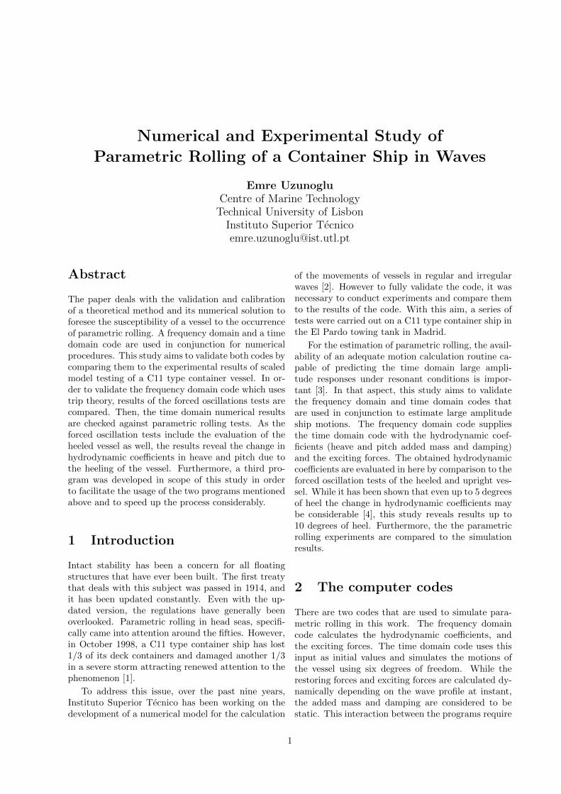
Figure 10: Load condition 1 polar plot

4.3 Polar Plots

With the help of the output from the intermediateprogram (the user interface) and MATLAB’s 3D sur-face plotting, it was possible to obtain polar diagramsfor the vessel. The advantage of polar diagrams isthat they represent simulation results for all headingsand speeds that the vessel is capable of. An exam-ple of these polar plots is presented in figure 10. Itrepresents the load condition and the wave height inwhich the numerical and experimental results were inbetter agreement (λ/Lpp = 1 and Hw = 4 meters).The polar plot represents 2821 simulations. Each twodegrees of heading was calculated (180, 178,... 2, 0)and the speeds were from 0 to 15 knots with a 0.5knot stepping (0, 0.5, 1 .... 14.5, 15 knots).

In the polar diagram presented, it can be seen thatparametric rolling starts at approximately 7 knotsand slowly wanes away at around 12 knots. Consider-ing this data, it can be stated that it is easier to slowdown to get out of the risky zone compared to speed-ing up out of it. Such polar diagrams can be devel-oped to examine the vessel’s proneness to parametricrolling in different load conditions and different wavesettings. This possibility was examined in this workand it was found that irregular waves polar plots de-viate from the regular waves results largely. Howeverthey still may be considered as a general assessmentfor the vessel.

5 Conclusions

In this study, results of the analysis of forced oscilla-tion tests and parametric rolling tests were comparedto the numerical results. The experimental data hasbeen obtained from model testing of a C11 type con-

tainer vessel which is known to be prone to parametricrolling. The comparison of the forced oscillation testsrevealed that strip theory generally fares well withheeling angles up to 10 degrees. The change in hy-drodynamic coefficients due to heeling was put underfocus and changes reaching 20% have been seen foradded mass and damping. This suggest that in cal-culation of the hydrodynamic coefficients, it may beimportant to do the calculation of these coefficientsiteratively for each time instant.

When the time domain code has been checkedagainst the experiments, it has been noted that therewere no false positives and the code does not reportparametric rolling in cases that they are not seen ex-perimentally. While its estimation is better for headseas, for following seas an adjustment of the meta-centric height ( therefore the stiffness) is necessary.Furthermore, an example polar plot has been intro-duced to allow the numerical assessment of paramet-ric rolling in all headings and speeds that the vesselis capable of. The production of these plots is im-portant to see which conditions are dangerous for thevessel. Even if irregular plots and regular plots can-not be related, they are important to see if the vesselis generally prone to parametric rolling in a certainloading condition.

References

[1] W N France, M Levadou, T W Treakle, J RPaulling, R K Michel, and C Moore. An investi-gation of head-sea parametric rolling and its influ-ence on container lashing systems. Marine Tech-nology, 40(1):1–19, 2003.

[2] S Ribeiro e Silva, T A Santos, and C GuedesSoares. Parametrically excited roll in regular andirregular head seas. International ShipbuildingProgress, 52:29–56, 2005.

[3] Sergio Ribeiro e Silva, Carlos Guedes Soares, An-ton Turk, Jasna Prpic-Orsic, and Emre Uzunoglu.Experimental assessment of parametric rolling ona C11 class containership. In Proceedings of theHYDRALAB III Joint User Meeting, pages 267–270, Hannover, February 2010.

[4] Sergio Ribeiro e Silva, E Uzunoglu, Carlos GuedesSoares, Adolfo Maron, and Cesar Gutierrez. In-vestigation of the hydrodynamic characteristicsof asymetric cross-sections advancing in regularwave. In Proceedings of the 30th InternationalConference on Offshore Mechanics and Arctic En-gineering (OMAE’2011), Rotterdam, 2011. PaperOMAE2011-50322.

10

numerical and experimental study of parametric rolling of

Documents