numerical and experimental study on ... - ufdc image array 2
TRANSCRIPT

1
NUMERICAL AND EXPERIMENTAL STUDY ON IMPROVING DIAGNOSIS IN STRUCTURAL HEALTH MONITORING
By
JUNGEUN AN
A DISSERTATION PRESENTED TO THE GRADUATE SCHOOL OF THE UNIVERSITY OF FLORIDA IN PARTIAL FULFILLMENT
OF THE REQUIREMENTS FOR THE DEGREE OF DOCTOR OF PHILOSOPHY
UNIVERSITY OF FLORIDA
2011

2
© 2011 Jungeun An

3
To my parents

4
ACKNOWLEDGMENTS
First of all, I would like to give special thanks and appreciation to Dr. Raphael T.
Haftka, the chairman of my advisory committee. I am grateful to him for providing me
with this excellent opportunity to complete my doctoral studies. I sincerely hope we will
remain in contact in the future. I would also like to thank to Dr. Nam-Ho Kim, co-
chairman of my advisory committee, for his valuable comments at our weekly meeting. I
would also like to thank to Dr. Mark Sheplak and Michael J. Daniels for their willingness
to review my Ph.D. research and to provide me with the constructive comments which
helped me to complete this dissertation.
I also wish to express my gratitude to Dr. Fuh-Gwo Yuan from North Carolina
State University, who worked together to provide a large share of knowledge and insight
to the future of our research. The experience he supplied me greatly contributed to this
dissertation.
I thank Dr. Byung Man Kwak from Korea Advanced Institute of Science and
Technology, who was my advisor during my PhD study in Korea, for kind and helpful
advice. He had shown a good attitude toward research. I also thank Dr. Hoon Sohn and
Mr. Chul-Min Yeum from Korea Advanced Institute of Science and Technology for
helping me to do the experiment. Since their great knowledge and experience in this
field helped me a lot, I had a wonderful opportunity to co-author a journal paper with
them.
I also thank to my colleagues at the Structural and Multidisciplinary Group of the
Mechanical and Aerospace Engineering Department of the University of Florida for their
support, friendship and many technical discussions.

5
I thank Rick Ross, Thiagaraja Krishnamurthy and Tzikang Chen from NASA for
their comments and question all along this research. I also thank the Air Force Office of
Scientific Research (Grant: FA9550-07-1-0018) and NASA (Grant: NNX08AC334) for
their great interest and funding of this research.
I also would like to express my deepest appreciation to my parents for their
emotional support.

6
TABLE OF CONTENTS
page
ACKNOWLEDGMENTS .................................................................................................. 4
LIST OF TABLES ............................................................................................................ 8
LIST OF FIGURES .......................................................................................................... 9
LIST OF SYMBOLS AND ABBREVIATIONS ................................................................ 13
ABSTRACT ................................................................................................................... 15
1 INTRODUCTION .................................................................................................... 17
Aircraft Maintenance and Its Impact on Safety ....................................................... 17
Structural Health Monitoring (SHM) ........................................................................ 19
Damage Diagnosis ................................................................................................. 21
Damage Severity .................................................................................................... 25
Damage Prognosis ................................................................................................. 26
Objective of This Research ..................................................................................... 28
How to Achieve the Objective ................................................................................. 29
2 BASIC PRINCIPLES ............................................................................................... 31
Lamb Wave Propagation in a Thin Plate................................................................. 31
Wave Equation ................................................................................................. 31
Wave Scatter .................................................................................................... 37
Piezoelectric Materials ............................................................................................ 39
Actuation Equation ........................................................................................... 40
Sensing Equation ............................................................................................. 42
Analytical Solution to a Toneburst Excitation .......................................................... 44
Wavefield Simulation [51, 54] ................................................................................. 53
Governing Equations of Flexural Waves .......................................................... 53
Finite Difference Algorithm ............................................................................... 55
3 IDENTIFYING CRACK LOCATION USING MIGRATION TECHNIQUE ................. 59
Migration Technique ............................................................................................... 59
Bayesian Approach ................................................................................................. 66
Bayesian Approach .......................................................................................... 66
Direct Image Intensity ....................................................................................... 69
Multivariate Normal Model about Center of Intensity ........................................ 70
Compensation for Geometrical Decay .................................................................... 73
Geometrical Decay in Plate Wave .................................................................... 75
Application to Migration Technique .................................................................. 77

7
Numerical Simulation ....................................................................................... 78
4 EXPERIMENTAL STUDY ON IDENTIFYING CRACKS OF INCREASING SIZE ... 82
Test Panel and Test Procedure .............................................................................. 82
Results .................................................................................................................... 88
Scattered Signal from the Damage .................................................................. 88
Variation of the Signal with Crack Size ............................................................. 88
Effect of Frequency .......................................................................................... 91
Crack Location Effect ....................................................................................... 94
Migration Technique with Experimental Data .......................................................... 96
5 BAYESIAN APPROACH TO IMPROVE DIAGNOSIS FROM PAST PROGNOSIS ........................................................................................................ 100
Modeling ............................................................................................................... 100
Improved Diagnosis by using Bayesian Approach ................................................ 104
Constructing Prior Distribution using Different Prognosis ..................................... 106
Perfect Prognosis ........................................................................................... 107
Uncertainty in Crack Propagation Parameters ............................................... 108
Prognosis using Least Squares Fit of Paris Law ............................................ 110
Prognosis using Least Squares (Non-Physics Model) .................................... 112
6 CONCLUSION ...................................................................................................... 116
LIST OF REFERENCES ............................................................................................. 117
BIOGRAPHICAL SKETCH .......................................................................................... 124

8
LIST OF TABLES
Table page 2-1 Properties of piezoelectric disc ........................................................................... 45
3-1 Estimation error due to different imaging techniques .......................................... 73
3-2 Comparison of accuracy, different imaging results. ............................................ 80
3-3 Comparison of imaging results ........................................................................... 80
4-1 Mechanical properties of aluminum plate ........................................................... 83
4-2 Properties of piezoelectric disc (modified PZT-4) ............................................... 83
4-3 List of crack sizes tested, (unit: mm) .................................................................. 83
4-4 Comparison of different imaging methods .......................................................... 96
5-1 Parameters related to simulated crack propagation. ........................................ 102
5-2 Comparison of accuracy with 10000 MCS ........................................................ 114
5-3 Comparison of accuracy with 1000 MCS when ΔN=25 cycles ......................... 115

9
LIST OF FIGURES
Figure page 1-1 Safety record from worldwide commercial jet fleet [1] ........................................ 17
1-2 Fatigue crack growth [2] ..................................................................................... 18
1-3 Structural Health Monitoring ............................................................................... 20
1-4 Pitch-catch method [8] ........................................................................................ 22
1-5 Pulse-echo method [8] ........................................................................................ 23
1-6 Phased array method [8] .................................................................................... 23
1-7 Migration technique [53] ..................................................................................... 24
1-8 Time of Flight Diffraction (TOFD) [34] ................................................................. 26
1-9 Fatigue crack size estimation [35] ...................................................................... 26
1-10 Applying crack propagation model to improve accuracy of detection results ...... 29
2-1 Axisymmetric structural waves in plates in cylindrical coordinates ..................... 32
2-2 Symmetric and antisymmetric particle motion across the plate thickness .......... 33
2-3 Typical wave speed dispersion curves for symmetric and antisymmetric waves. ................................................................................................................ 36
2-4 Wave reflection from a small cavity .................................................................... 37
2-5 Circular piezoelectric actuator ............................................................................ 40
2-6 Hole detection problem. ...................................................................................... 45
2-7 Five peaked toneburst excitation sent to the actuator (110 kHz) ........................ 46
2-8 PZT actuator attached to an aluminum plate ...................................................... 47
2-9 Displacement at the boundary of the PZT (r=a) .................................................. 48
2-10 Displacement field induced by the piezoelectric actuation. ................................. 50
2-11 Scattered displacement response at r=113.4 mm from the cavity center. .......... 51
2-12 Electric signal obtained at the sensor position .................................................... 51

10
2-13 Comparison with experimental data ................................................................... 52
2-14 Snapshot of the simulated structural wave ......................................................... 57
2-15 Finite difference solution compared with wave propagation analysis ................. 58
3-1 Cross-correlation coefficient used to find the time difference between excitation and scattered signal in migration technique. ...................................... 60
3-2 Actuator and sensor positions for migration technique ....................................... 61
3-3 Excitation signal .................................................................................................. 63
3-4 Scattered wavefield and incident wavefield for back propagation....................... 64
3-5 Final images obtained by evaluating the image intensity at each point from simulation for a 50mm straight horizontal crack. ................................................. 65
3-6 Combining image using direct image intensity as likelihood ............................... 70
3-7 Estimation error in x and y directions. ................................................................. 71
3-8 Combined image using multivariate normal model. ............................................ 72
3-9 Possible errors related to geometrical decay ...................................................... 74
3-10 Signal decay with respect to wave propagation in plate ..................................... 76
3-11 An example of compensated signal displayed on time scale. ............................. 77
3-12 Images from migration technique with the same sensor data. ............................ 79
3-13 Image intensity distribution for a single actuator image ...................................... 80
4-1 Layout of actuators and sensors ......................................................................... 84
4-2 Damage manufactured to the plate .................................................................... 84
4-3 Signal generation and acquisition in the experimental set-up ............................. 85
4-4 Test procedure for estimated location by migration technique and signal amplitude measurement ..................................................................................... 86
4-5 Frequency sweep experiment. ............................................................................ 87
4-6 Toneburst excitation measured from all eight sensors from simulation and experiment. ......................................................................................................... 89
4-7 Experimental scattered signal amplitude change in different size cracks. .......... 90

11
4-8 Signal amplitude variation (maximum peak-to-peak amplitude). ........................ 91
4-9 Scattered signal amplitude with 150kHz excitation. ............................................ 92
4-10 Signal amplitude variation (maximum peak-to-peak amplitude). ........................ 93
4-11 Different crack center location with respect to the actuator positions: second crack center location is (-100mm, -140mm) ....................................................... 95
4-12 Scattered signal amplitude variation for cracks growing at a different location excited by 110 kHz ultrasonic toneburst. ............................................................ 95
4-13 Reconstructed scattered wavefield ..................................................................... 97
4-14 Experimental result is reproduced into image using migration technique. .......... 97
4-15 Combination of all 7 actuators available in the experiment. ................................ 98
5-1 Aircraft fuselage ................................................................................................ 101
5-2 Simplified loading condition .............................................................................. 101
5-3 Crack propagation. ........................................................................................... 103
5-4 Sample of detected estimated crack sizes (based on Eq.5-3) .......................... 104
5-5 Simulation procedure ........................................................................................ 106
5-6 Probability distribution function of crack size updated at every 50 cycles ......... 108
5-7 Crack size found by Bayesian update .............................................................. 108
5-8 Probability distribution function of crack size updated at every 50 cycles with uncertain parameters C and m. ........................................................................ 109
5-9 Crack size found by Bayesian update with uncertain C and m ......................... 109
5-10 Approximation of the inspection data by Least squares fit of Paris law with 95% prediction bounds. .................................................................................... 110
5-11 Estimated crack size by least square fitting of Paris law at each inspection cycle ................................................................................................................. 111
5-12 Demonstration of the suggested method to estimate crack size by Bayesian approach using prognosis based on least squares ........................................... 111
5-13 Approximation of the inspection data by 4th order polynomial with 95% prediction bounds. Only 40 recent data are used for curve fitting. .................... 113

12
5-14 Estimated crack size by least square fitting using a quartic polynomial at each inspection cycle ....................................................................................... 113

13
LIST OF SYMBOLS AND ABBREVIATIONS
A Signal amplitude
a Crack size
ai Initial crack size
C, m Crack propagation parameters
c Phase velocity of a Lamb wave
cg Group velocity of a Lamb wave
cL Pressure wave velocity
cT Shear wave velocity
D3 Electrical displacement in z-direction (charge per unit area)
d Plate thickness
d31, d33 Piezoelectric coupling constant
E3 Electric field in z-direction
ε Mechanical strain
FFT Fast Fourier Transform
H Heaviside step function
Hn Hankel functions
iFFT inverse FFT
Ii Image intensity from ith simulation or experiment
Id-corr Adjusted image intensity by geometrical decay compensation
Jn Bessel functions
k Wave number
l Likelihood
λ, µ Lamé constants
N Number of cycles

14
ν Poisson’s ratio
NDE Non destructive evaluation
PZT Lead zirconate titanate, a ceramic perovskite material that shows a marked piezoelectric effect.
RUL Remaining useful life
SHM Structural health monitoring, an automated inspection and maintenance system development
sE Mechanical compliance
σ Mechanical stress
TOF Time of flight, time difference between excitation signal and scattered signal
Φfg Cross-correlation (coefficient)
ω Angular frequency

15
Abstract of Dissertation Presented to the Graduate School of the University of Florida in Partial Fulfillment of the Requirements for the Degree of Doctor of Philosophy
NUMERICAL AND EXPERIMENTAL STUDY ON IMPROVING DIAGNOSIS IN
STRUCTURAL HEALTH MONITORING
By
Jungeun An
August 2011
Chair: Raphael Tuvia Haftka Major: Aerospace Engineering
Structural Health Monitoring (SHM) is a procedure of assessing structural integrity
during its service period to improve maintenance in terms of cost and reliability. In SHM
for aircraft applications, crack identification using reflected ultrasonic Lamb waves from
a crack is one of the most active research areas. In addition to detecting a crack,
estimating its size is important for judging the severity of the damage, and this can be
done by various techniques. Specifically, we focus on the relationship between the
sensor signal amplitude and crack size through experiments and simulation for help in
size estimation. The maximum received signal amplitude is found to vary linearly from
simulation and this agrees with measurements with crack size up to 30 mm.
However, SHM using embedded sensors have limitation in terms of accuracy of
detection. Our approach to overcome this is as follows. If measurements are frequently
performed using the above mentioned techniques while the crack grows, then a better
estimation of crack size may be possible by analyzing sensor signals for the same crack
location at different sizes.
The main objective of this research is to improve the accuracy of current diagnosis
by using the prediction from previous inspection results. Unlike manual inspection, SHM

16
can take frequent measurements and trace crack growth. By taking advantage of this
aspect, higher accuracy about current crack size can be achieved. First, using the
previous SHM measurements and the crack propagation model, we predict the
statistical distribution of crack sizes at the next SHM inspection cycle. Then, this
predicted distribution is combined with the SHM measurement at the next cycle by using
the Bayesian approach for more precise estimate. The propagated distribution from the
previous inspection is used as a prior and the variability at the current inspection is used
to build the likelihood function. The uncertainty in measurements is modeled by a
lognormal distribution. Results show substantial improvements in accuracy.

17
CHAPTER 1 INTRODUCTION
Aircraft Maintenance and Its Impact on Safety
The importance of proper maintenance to prevent fatigue failure is a key issue for
all mechanical components in an airplane. As shown in Figure 1-1, major catastrophic
failures of aircrafts come from lack of maintenance and repair rather than design errors
in commercial jet fleets [1].
Figure 1-1. Safety record from worldwide commercial jet fleet [1]
Fatigue crack growth is one of the most common types of failure in an aircraft
since the safety factor of designed aircraft is relatively low, and the aircraft is subjected
to many different types of cyclic loadings during its service period. Cracks usually start
from inherent material defects or micro-cracks, increase their size by cyclic loadings,
and eventually lead the structure to fail.
Many crack propagation models are proposed to describe the behavior of fatigue
crack growth. Fatigue cracks usually propagate very slowly in the beginning, but the

18
Figure 1-2. Fatigue crack growth [2]
propagation speed increases exponentially with time. Since the cracks in the beginning
stage are too small to detect, most inspection methods focus on the stable crack growth
stage (refer to Figure 1-2).
In FAA regulations, inspections of an aircraft in service should be scheduled on an
annual basis to maintain structural safety [3]. Under current approach, the aircraft is
inspected under fixed schedule in order to replace panels with any sub-millimeter size
cracks that might become dangerous before the next inspection. This is called manual
inspection, or preventive maintenance. The aircraft is sent to a hanger, and damaged
panel in an aircraft is identified using several inspection techniques and replaced. The
cost for this procedure includes downtime of the aircraft and high labor costs. Since the
number of panels that are replaced during the entire service period of an airplane is

19
about 2 – 3%, most of cost is spent on inspecting panels that do not have cracks with
significant size.
To prevent all possible failures between inspections, the manual inspection
procedures should be very accurate. In fact, the current state-of-the-art manual
inspection procedure is so accurate that some of sub-millimeter cracks within the
structure can be detected during the inspection [4]. However, manual inspection is very
costly and time consuming, and there are ―hot-spots‖ where the reliability is crucial but
inspectors cannot access easily during the manual inspection procedure. If we can
automate the inspection procedure, the diagnosis of current health status of the
structure under operation can be more reliable. As a result, we can reduce the overall
costs and obtain a better knowledge about the possible failure of the structure
simultaneously.
This is the reason for interest in condition-based maintenance over preventive
maintenance. Structural health monitoring (SHM) is an enabling technology that can
detect, diagnose, and predict the structural behavior under unsupervised modes. There
is great interest in developing SHM using embedded sensors as an alternative for
manual inspection [5-45]. The next section will explain the basic concepts of SHM,
followed by literature review on damage diagnosis and prognosis.
Structural Health Monitoring (SHM)
Structural health monitoring (SHM) is an integrated technology of assessing
structural damage using an automated procedure. The importance of SHM is currently
increasing because of economic and safety reasons.

20
Figure 1-3. Structural Health Monitoring
As shown in Figure 1-3, SHM consists of diagnosis and prognosis. Diagnosis in
SHM processes the signal from embedded sensors to detect the damage. When
damage is found, prognosis uses a crack propagation model to find out the future
behavior of the damage and whether the part needs maintenance or not.
Initially the development of SHM technologies focused on damage detection using
embedded sensors, and progressively moved toward the future behavior of the
damage. With SHM systems, we can perform the damage assessment at any time, so
that the system can execute continuous monitoring of the structure. Using the monitored
data from SHM systems, we can predict the damage growth and design the
maintenance schedule in accordance with the most critical damage for an airplane.
The main advantage of SHM is that we can perform condition-based maintenance
by following crack propagation, thereby substantially increasing the average time

21
intervals between downtime between maintenance and reducing the total number of
replaced panels during the entire service period of an aircraft [45].
Damage Diagnosis
Damage diagnosis refers to the procedure of identifying the current damage state.
This includes damage detection, material property characterization, and determination
of dangerous spots. For an automated procedure of diagnosis, several non-destructive
evaluation (NDE) techniques have been developed by many researchers. Modern NDE
techniques include radioscopy, ultrasonic guided wave scanning, shearography, dye
penetrant testing, magnetic resonance imagery, laser interferometry, acoustic
holography, infrared thermography, fiber optics and eddy-current [6-26]. Among them,
ultrasonic guided wave based methods are very popular and widely developed and
used since they have several advantages such as better sensitivity to local damage [6-
11]. They are cheap, easy to implement, and enable active sensing and monitoring.
They use piezoelectric transducers for excitation of Lamb waves, which are a type of
structural waves in plate structures. Lamb waves are guided by two parallel free
surfaces, and their wavelengths are of the same order of magnitude as the thickness of
the plate [7].
Currently developed techniques using ultrasonic wave include pitch-catch, pulse-
echo, phased array, and migration technique [8-10]. Basic measurements for all of
these techniques include the time of flight (TOF), phase change, frequency and
amplitude change, and angle of wave deflection. Among them, the time of flight, which
indicates the time difference between excitation and sensing, is the most reliable in
locating the damage; so many methods rely on this property.

22
The pitch-catch method detects damage from the changes in the Lamb wave
traveling through the damaged region. The change in the wave propagation path due to
damage causes the difference between the healthy state and damaged state. This
method uses transducers in pairs: transmitter and receiver. The difference in the
structural wave traveling from transmitter and receiver evaluates the damage located
between this pair. The process is shown in Figure 1-4. In general, this method is good
for determining the damage existence, but is not sensitive to location or size of the
damage. To overcome these difficulties, many researchers have proposed several
methods in this category [21].
Figure 1-4. Pitch-catch method [8]
The pulse-echo method (Figure 1-5) relies on the scattered wave from damages to
detect them. The transmitters and receivers are located on the same side of the
damage to evaluate reflection in this method. If the velocity of the Lamb waves is
known, we can calculate the distance from which the location of damage can be found.
This method provides wider coverage with the same set of actuator-sensor pairs, and
the TOF is more sensitive to the location of damage than pitch-catch method. However,
since the scattered signal is much smaller than the original excitation, it may easily be
contaminated by noise. Although no significant improvements have been made on the
method itself, pulse-echo is still widely used in many SHM applications [9].

23
Figure 1-5. Pulse-echo method [8]
The phased array method (Figure 1-6) is adopted from the principles used by the
radar systems. Many excitation sources located in a compact region send Lamb waves
with different frequencies at the same time. Then the phase change in the received
signal forms an image, in which the maximum phase change indicates the possible
location of damage. This method is suitable to examine inner structural damage in a 3-D
medium. Many researchers have tried to improve this technique, and there is a wide
variety of phased array methods available for different applications. [8, 31]
Figure 1-6. Phased array method [8]
The migration technique (Figure 1-7) is one of the most powerful tools to detect
damage in a structure. Its basic principle is almost the same as pulse-echo technique,
but the major difference is that we find the cross-correlation between the excitation and

24
scattered wave to accurately find the location of damage. A solid foundation of the
migration technique has been established over nearly a decade [51-56]. Since damage
identification used in this work is based on the migration technique, this method is
explained in detail in Chapter 3.
Figure 1-7. Migration technique [53]
There are many other techniques to identify damage within a structure, but every
active monitoring technique using ultrasonic wave is classified into one of the categories
in terms of sending and receiving signals. For example, the time reversal technique
whose biggest advantage is no requirement for baseline information is a type of pitch-
catch algorithm [32], and methods employing sensor network are a hybrid form of pitch-
catch and pulse-echo techniques [37, 38].
There are several other techniques that produce results in the form of images [39-
42]. For example, DORT method is developed based on time reversal operator and
there is an attempt to apply tomography to SHM [40]. L-SAFT processing technique
produces modified B-scan type images of Lamb wave inspection results [42].

25
Damage Severity
The term ―damage severity‖ can indicate many different aspects of a flaw. A
severe damage can be a flaw at the most critical location with structural load, or it can
be a huge flaw at a relatively less critical location. Although there is no objective
measure of severity, the size is usually the most important information for assessing
damage severity. Since the location of a flaw is closely related to the size, the size
estimation does not have a meaning when we do not know the location of damage [5].
This is why most of current research for two dimensional applications focuses more on
the existence or location of damage rather than accurate quantification. However, there
have been techniques to estimate damage size using ultrasonic wave or change in the
natural frequency when the approximate location of the damage is known. Time of flight
diffraction (TOFD) is a well known approach of estimating the defect size and location in
beams by embedded PZT sensors [34]. The diffracted signal is measured at the
receiver to estimate the size of a crack as shown in Figure 1-8.
Also, several other approaches were used for beam structures. Fromme [35]
demonstrated a fatigue crack growth in a beam by using the change in the reflected
signal, and compared it with simulation results. He demonstrated that the signal
amplitude and crack size are related, but the signal amplitude might not be accurate
enough to determine crack size by comparison between simulation and experiment
(Figure 1-9).
Currently, the estimation of flaw size is not ready for real-life implementation yet.
Sohn et al. [7] mentioned that the crack sizes are obtained with errors that can be as
large as 21% even for a beam. The size estimation part is of great interest to most
developers in SHM.

26
Figure 1-8. Time of Flight Diffraction (TOFD) [34]
Figure 1-9. Fatigue crack size estimation [35]
Damage Prognosis
Prognosis is a process to make a prediction about the future behavior of damage.
This includes remaining useful life (RUL) estimation, crack propagation behavior

27
prediction and the adjustment of maintenance schedule. . If accurate RUL can be
estimated, the propagation of cracks and the next maintenance schedule can easily be
calculated. Therefore, the research in prognosis naturally focuses on accurately
estimating the RUL. In general, prognosis requires a good knowledge on the
uncertainties in the detection capabilities, average and prospective loading, and
material properties that governs damage growth. Because of these uncertainties, RUL
should be modeled as a statistical distribution.
The research on prognosis has several challenges. Estimated future loadings and
estimated crack size contain large uncertainty, and the crack propagation model is not
exact. Despite all these practical difficulties, research on prognosis is vigorous these
days. Started from Paris’ law [74] in early 1960’s, the crack propagation model has
experienced rapid advances. Elber [75] observed that the effect of crack closure is
important, and the model using effective range of stress intensity factor was developed
by Paris et al. [74]. Recent developments in crack propagation model include universal
model of Paris’ law [76] and NASGRO model that can be used with more number of
parameters.
Since there is no actual SHM system installed on an aircraft, most research on
prognosis relies on conceptual SHM system. Kulkarni and Achenbach [59] have
analyzed a conceptual SHM system to quantify the effects of imperfect inspections
during the growth of a macrocrack. However, the effort to implement SHM in a practical
system is being developed, and many researchers estimated the RUL through several
examples. For example, Wang and Youn [60] have applied real time prognostics and
health management to estimate RUL in a statistical manner. Also, on-line structural

28
health monitoring strategy has been applied to integrated prognosis model by Mohanty
et al. [61]
This work employs prognosis model for predicting future behavior. Paris’ law for
relatively simple example is encountered for improving diagnosis. We also considered
data-driven models for prognosis.
Objective of This Research
The objective of this work is to develop a diagnosis method to identify crack
information using ultrasonic wave, and explain how to make the diagnostic result more
accurate by employing past prognosis information. From the diagnosis result, it is
possible to obtain information of current crack such as its location and size. During
regular inspection cycles, those inspection results are used to make a prediction about
the crack size at the next inspection (prognosis). This forms a prior knowledge about the
crack size before we actually take the measurements. When we have the measurement
at the corresponding cycle, the current crack size is estimated by combining the prior
knowledge with the inspection data. Therefore, the main objective of this research is to
provide a framework that incorporates the crack propagation model to improve size
estimation result (Figure 1-10).
The current developments of SHM system consider the diagnosis and prognosis
as two separate procedures (Figure 1-3). However, we can improve the diagnosis by
using the crack propagation model and current inspection as a predictor-corrector
concept. We bring the crack propagation model into the loop of diagnosis to improve
diagnosis result.

29
Figure 1-10. Applying crack propagation model to improve accuracy of detection results
How to Achieve the Objective
Accurate location of the damage should be known prior to estimating damage
severity. Chapter 3 explains migration technique, a popular method used to estimate the
location of damage. Section 3.1 presents migration technique developed by Dr. Yuan.
On the basis of what he has achieved, various approaches are described to improve the
identification of crack location in Section 3.2 and 3.3.
One of the measures of damage severity is the length of a crack. This is essential
information required to move on to the prognostic stage. There have been researches
on increasing signal strength due to longer or bigger cracks. Chapter 4 describes the
relation between crack size and signal amplitude by comparing simulation with
experiment. Simulation tool described in Section 2.4 is provided by Dr. Yuan.

30
In Chapter 5, we assume a situation where we have measurement uncertainty,
and we have to estimate the size from uncertain data. With a hypothetical SHM system,
a simulation result of fuselage panel is presented. Section 5.2 explains how to apply
Bayesian approach to this problem. The Bayesian approach for this application uses
current inspection results to form a likelihood function and previous result to construct a
prior distribution. By combining those two, a more accurate result can be obtained.

31
CHAPTER 2 BASIC PRINCIPLES
For various active monitoring applications, structural wave propagation by
piezoelectric actuator/sensor is often used. In this chapter, some basic concepts are
introduced related to the wave propagation in plates and piezoelectric behavior. Section
2.1 discusses some issues related to Lamb wave propagation and the behavior of
scattered wave from damage, and Section 2.2 discusses the behavior of piezoelectric
materials with respect to the electric field applied to the actuators and strain applied to
the sensors. Section 2.3 presents an example of exciting Lamb wave and detecting the
scattered wave using a piezoelectric patch. Excitation of PZT material uses the
actuation equation described in Section 2.2, propagation and scatter use the solution to
the wave equation explained in Section 2.1, and sensing of electrical signal uses the
sensing equation described in Section 2.2. By comparing the analytical approach to the
experimental result, we found a good agreement in the shape of detected signals.
Section 2.4 introduces a finite difference algorithm we have used to simulate the
damage detection problem.
Lamb Wave Propagation in a Thin Plate
Wave Equation
Lamb waves are structural ultrasonic waves that are guided between two parallel
free surfaces. Two basic types of Lamb wave, symmetric and antisymmetric, can exist
in the plate. The movement of a particle for symmetric Lamb wave resembles pressure
wave, whereas it resembles shear wave for antisymmetric Lamb wave (Figure 2-1).
Lamb waves are highly dispersive, and their speed depends on the product of

32
frequency and the plate thickness. This section explains the stress and strain behavior
within a plate when Lamb waves induced by external excitation propagate within the
plate.
First assume a simple case where we have an infinite plate with thickness 2d, and
the wave is propagating from the origin (Figure 2-1). To describe the displacement
behavior of particles induced by wave propagation, Navier’s governing equation [8] for
equation of motion in cylindrical coordinates is as follows (No body forces):
22
2 2
22
2
( )
( )
r rr
zz
u uu
r r t
uu
z t
(2-1)
Under the axisymmetric assumption, the equations can be described as θ-
invariant. λ and µ are Lamé constants, ρ is density, r z
r k is the gradient
operator,2
2
2
1r
r r r z
is the Laplace operator, and r r zu u u
r r z
is the
divergence term.
Figure 2-1. Axisymmetric structural waves in plates in cylindrical coordinates. It may be misleading, but uz is present for the pressure wave because of the displacement induced by Poisson’s ratio.

33
The speed for each mode of Lamb wave is described by:
2(pressure wave)
(shear wave)
L
T
c
c
(2-2)
There are two independent solutions for the wave equation, each corresponds to
pressure and shear wave, described by symmetric and antisymmetric modes,
respectively. For each mode, the reference coordinates for the direction of particle
motion are shown in Figure 2-2. Particle movement for the symmetric mode of Lamb
wave is symmetric with respect to the mid plane of the plate, while it is opposite for the
antisymmetric mode.
Figure 2-2. Symmetric and antisymmetric particle motion across the plate thickness
Wave number analysis decomposes the signal shape into the sum of cosine and
sine waves in the form of i t
zu e . There exist many different angular frequencies for
an excitation if the excitation is not a simple harmonic function, and each of them has a
different solution. The solution of Eq.2-1 corresponding to the excitation i t
zu e
is
available in the literature [9,46,47]:

34
* 2 2 2
1
* 2 2
0
* 2 2 2
1
*
2 cos cos ( )cos cos ( )( )
2 cos cos ( )cos cos ( )
2 sin sin ( )sin sin ( )
2 sin sin (
i t
r
i t
z
i t
r
z
u A k q qd pz q k q pd qz J kr eSymmetric
u A kpq qd pz k k q pd qz J kr e
u A k q qd pz q k q pd qz J kr e
u A kpq qd pz k k
2 2
0
( ))sin sin ( ) i t
Antisymmetricq pd qz J kr e
(2-3)
where A* is an arbitrary constant calculated by applying initial and boundary conditions,
2 2
1 , 1 ,L T
c cp k q k c
c c k
is the phase velocity, J0, J1 are Bessel functions, ω
is the angular frequency, and k is the wave number. For a general input signal, we have
many different frequency components of ω for modified wave number analysis.
Corresponding k are found by considering the wave velocity.
The solution in Eq.2-3 implies that the amplitude of a circular crested wave in a
plate experiences a decay described by Bessel function in space.
One important property of Lamb wave is that there are several propagation
modes. Each mode has different frequency due to different wave number, and the wave
velocity can be calculated from its characteristic equations. To derive the characteristic
equation, the traction free boundary conditions should be considered. The strain
components induced by this displacement field are listed as follows:
1 1
2
1 1
2
1 1
2
r rrr r
r r zrz
z zzz z
u uu u
r r r r
u u u u
r r z r
uu u
z z r
(2-4)

35
To introduce the boundary conditions for the upper and lower free surfaces of the
plate, the stresses can be derived from:
2
2
zz zz
rz rz
(2-5)
Then, the characteristic equation for the symmetric and antisymmetric wave are
obtained by applying ( ) 0, ( ) 0zz rzd d :
2
2 2 2
2 2 2
2
tanh( ) 4( )
tanh( ) ( )
tanh( ) ( )( )
tanh( ) 4
iqd pqkSymmetric
ipd k q
iqd k qAntisymmetric
ipd pqk
(2-6)
There is another important property of the Lamb wave, which is the traveling
speed of Lamb wave packets, such as the one limited by a Hann window. Hann window
is a type of window function, which is zero-valued outside of some chosen interval. The
traveling speed of Lamb wave packets is called the group velocity, and calculated from
the phase velocity c.
1
2
( )g
cc c c d
d
(2-7)
The wave speed dispersion curves in an aluminum plate are shown in Figure 2-3.
The figure is generated using Lambwave_UI developed by Yuan et al [55].
From Figure 2-3, we know that the wave velocity depends on the frequency. The
relationship between wave velocities in the plate and frequency is inherent material
properties. The wave propagation analysis depends on the wave velocity, which is used
to calculate the wave number for the corresponding propagation mode.

36
A
B
Figure 2-3. Typical wave speed dispersion curves for symmetric and antisymmetric waves. A) Phase velocity B) Group velocity
S0
S1
S2
A0
A1
A2
S2
A1
A0
S0
S1
A2

37
Wave Scatter
When a Lamb wave hits a defect, it scatters around the defect as if the defect is a
secondary source. The amplitude of scattered wave depends on the direction, mode
(symmetric or antisymmetric), wave number, and frequency. The simplest way to model
the scatter from an arbitrary shaped damage is by analyzing an infinitesimal cavity in
the wave propagation path, and using Huygen’s principle [48] to model the wave front
and corresponding amplitude. Huygen’s principle for reflection describes the scattered
or diffracted wave as a sum of reflections from many secondary sources on the
reflection boundary. Consider a small cavity of radius a standing in the path of the wave
propagation, as shown in Figure 2-4.
Figure 2-4. Wave reflection from a small cavity
The equation of motion for a simple wave is:
2
2
22
2 2
10
1 1
r r
T
r rr
u uc
u uwhere u r
r r r r
(2-8)

38
In this case, both the incident wave and scattered wave exist. Denoting the
displacement field induced by incident wave as ui and scattered wave as us, the
displacement field is given by ur= ui + us.
The incident wave can be expressed through Bessel function [49]:
0 0
0
( 1) ( )cos ( 1, 2)n
i n n n
n
u U J kr n
(2-9)
where Jn(kr) are the Bessel functions, U0 is a constant related to the magnitude of the
incident wave, and k=ω/c is the wave number.
When the incident wave interacts with the cavity, a scattering field will result.
Substituting the scattered wave ( , ) i t
s su U r e to Eq. 2.8., the solution for the wave
equation for the scattered wave can be written as [47]:
(2)
0
( , ) ( )cos i t
s n n
n
u r A H kr n e
(2-10)
To find the coefficients An, we need to consider the traction-free boundary
conditions on the cavity surface:
0
0
12
1
rr r
r r rrr
r
at r a
r
uu u u
r r r r
u uu
r r r
u
(2-11)
The total displacement field ur= ui + us should satisfy the boundary conditions.
(2)
0
0
0
( ) ( )( 1) cos 0
i s
n n nn n
n
u uat r a
r r
dJ kr dH krU A n
dr dr
(2-12)

39
Because functions cos nθ are orthogonal, we find the coefficient values An from
Eq.2-10 as follows:
0
(2)
( 1) '( )
( )
n
n nn
n
U J kaA
H ka
(2-13)
The scattered field has the form of Eq.2-10 with coefficients in Eq.2-13. In the far
field, using an asymptotic expression, the result can be written as:
0
2( , , ) exp ( )su r t U i t kr S
kr
(2-14)
This implies that the wave decays with respect to time, and the amplitude is
proportional to 1/√kr. Also, the amplitudes depends on the angle via S(θ). There is no
general analytical solution for S(θ), but it can be calculated numerically. Graff has
shown several numerical results of the structural wave scattering [49] when the size of
cavity is of the same order of magnitude with the wavelength.
Piezoelectric Materials
Piezoelectricity, by definition, is a property of certain materials to physically deform
in the presence of an electric field or, conversely, to produce an electric charge when
mechanically deformed. There are a wide variety of materials that exhibit this
phenomenon. When we applied electrical field to those materials for polarization, the
material becomes permanently elongated in the direction of the poling field (polar axis)
and correspondingly reduced in the transverse direction. Applying a voltage in the
direction of the poling voltage produces further elongation along the axis and a
corresponding contraction in the transverse direction obtained from its Poisson’s ratio.

40
Actuation Equation
Piezoelectric material couples the electrical and mechanical effects through the
piezoelectric constitutive equations. The ability to generate mechanical strain from
applied electric field is modeled using actuation equation in polar coordinates [8]:
3 3
3 3
E E
rr rr rr r r
E E
r rr
s s d E
s s d E
(2-15)
where ε is the mechanical strain, σ is the stress, E is the electric field applied to the
piezoelectric material, Es is the mechanical compliance of the material measured at
zero electric field (E=0), and d is a material property representing the piezoelectric
coupling effect.
The remainder of this section will derive the displacement field generated by a
circular piezoelectric actuator attached on a plate. Consider an isotropic circular
piezoelectric actuator (Figure 2-5), which undergoes uniform radial and circumferential
expansion, the strain-displacement relation in polar coordinates reduces to:
0
rrr
r
r
u
r
u
r
(2-16)
Figure 2-5. Circular piezoelectric actuator

41
The piezoelectric coupling constant and mechanical compliance are identical in
planar directions (orthogonal to polarization direction):
3 3 31
11 12,
r
E E E E E
rr r
d d d
s s s s s
(2-17)
where subscript 3 denotes the z-direction (polarization)
Solving Eq.2-15 for σ yields:
31 3
2
11
31 3
2
11
(1 )
(1 )
(1 )
(1 )
rrrr E
rr
E
d E
s
d E
s
(2-18)
where ν is the Poisson ratio defined as 12
11
E
E
s
s . By the displacement-strain
relationship in Eq.2-16, the stresses can be expressed in terms of displacements:
31 32
11
31 32
11
1(1 )
(1 )
1(1 )
(1 )
r rrr E
r r
E
u ud E
s r r
u ud E
s r r
(2-19)
Newton’s law of motion applied to an infinitesimal element yields:
2rrrrr
du
dr r
(2-20)
Therefore, the following wave equation can be obtained:
22
2 2 2
11
1 1
(1 )
r r rrE
d u du uu
s dr r dr r
(2-21)
Using the wave velocity 2
11
1
(1 )P E
cs
and the wave number k=ω/cP, the
equation becomes:

42
2
2 2 2
21 0r r
r
d u dur r k r u
dr dr
(2-22)
which is the Bessel differential equation of order 1.The general solution for Eq.2-22 is:
1( ) ( )ru r A J kr (2-23)
The constant A is determined from boundary conditions. For stress-free boundary
conditions at r=ra, we have:
31 32
11
1 1 31 3
31 3
0 1
1( ) (1 ) 0
(1 )
'( ) ( ) (1 )
(1 )
( ) (1 ) ( )
r rrr a E
a a
a
a a a
u ur d E
s r r
AkJ kr AJ kr d Ea
r d EA
kr J kr J kr
(2-24)
So the displacement induced by circular piezoelectric actuator is:
131 3
0 1
(1 ) ( )( )
( ) (1 ) ( )r a
a a a
J kru r r d E
kr J kr J kr
(2-25)
This implies that at a given radial location, the displacement amplitude is
proportional to the applied electric field. Many manufacturers of piezoelectric devices
provide wide range of linearity that this relation can be applied within its normal
operation condition.
Sensing Equation
Similarly, piezoelectric materials respond to mechanical strain to generate electric
field within them. The process of generating electric field from stress is described by
sensing equation [8]:
3 3 3 3
T
r rr k kE g g D (2-26)

43
where gij is the piezoelectric voltage coefficient and represents how much electric field is
induced per unit stress, D is the electrical displacement (charge per unit area), and βjk is
the inverse of the permittivity coefficient e.
The piezoelectric coefficients have following identities:
T
iq ik kq
T
ip ik kq
T T
ik kj ij
g d
d e g
e
(2-27)
Consider an isotropic disc, Eq. 2.26 can be stated as:
3 31 31 33 3
T
rrD d d e E (2-28)
Then recall Eq.2-19,
31 32
11
31 32
11
1(1 )
(1 )
1(1 )
(1 )
r rrr E
r r
E
u ud E
s r r
u ud E
s r r
(2-29)
Substituting this to Eq.2-28,
2
31 313 33 3
11 11
21( )
(1 ) (1 )
T
rE E
d ddD ru e E
s r dr s
(2-30)
Eq.2-30 defines the relation between induced displacement ur and electrical field
generated in piezoelectric sensor. If there is no external electric field, the electric
displacement within the piezoelectric dipole can be described with the first term of Eq.2-
30. Note that uz is the dominant particle movement, but the stress applied to the PZT
sensor is related only to ur. To obtain the voltage from the electric displacement, the
charge is obtained by integrating D, and by dividing with capacitance of the PZT sensor,
we can obtain the voltage difference.

44
3D dzQV
C C
(2-31)
However, the stress field within the piezoelectric sensor is not uniform and not
easy to analyze. Assuming the size of PZT sensors is smaller than the wavelength, we
can use a pin-point approximation for the sensor for the central displacement [8].
Analytical Solution to a Toneburst Excitation
An analytical analysis on the problem of flaw detection should include all the
previous concepts to explain the wave behavior. To summarize all the basic concepts to
simulate a problem of flaw detection, a practical example is introduced in this section. In
an infinite plate with thickness 3.2 mm, one PZT actuator is attached at the origin of the
plate, and the signal is obtained at the same position. We excite the plate using a
toneburst signal for successful generation of Lame wave of 110 kHz. 110 kHz is
determined to have the maximum response for A0 wave from the experiment (Also
explained in Chapter 4). The dimensions and material properties of PZT actuator are
listed in Table 2-1. It is assumed that there is one through-the-thickness hole of 2 mm
diameter, located 113.4 mm from the PZT center.
The procedure to find an analytical solution to the problem is shown in Figure 2-6B.
When we apply voltage to the PZT actuator, it generates displacement field by actuation
equation (Eq.2-15). Wave propagates the space between the actuator and damage, and
the displacement field is described by wave propagation equation (Eq.2-3). When the
wave hits the damage, it is scattered and the scattered wave solution is found using
Eq.2-10. Finally, the PZT sensor detects the scattered wave, and it generates electric
signal described by the sensing equation (Eq.2-25).

45
A
B
Figure 2-6. Hole detection problem. A) Problem layout B) Flowchart for analysis
Table 2-1. Properties of piezoelectric disc (modified PZT-4)
Geometry (mm) diameter:10.0, thickness:0.4 Density ρ (kg/m3) 7.9 × 10³ Young’s modulus E (GPa) E11: 86, E33: 73 piezoelectric coefficient d31 (m/V) -140 × 10-12 Piezoelectric coefficient d33 (m/V) 320 × 10-12 Piezoelectric coefficient g31 (Vm/N) -11 × 10-3 Piezoelectric coefficient g33 (Vm/N) 25 × 10-3 Dielectric constant K3 1400
We review only the fundamental A0 mode in this section. Similar analysis can be
made for higher antisymmetric modes or symmetric modes by changing the wave
velocity to corresponding mode. The excitation signal is 5 count toneburst shown in

46
Figure 2-7 and Eq.2-32. The sampling frequency is 5 MHz.
0 20 40 60 80 100-10
-5
0
5
10
Time (s)
Sig
nal (V
)
A0 50 100 150 200 250 300
0
10
20
30
40
50
60
Frequency (kHz)
Magnitude
B
Figure 2-7. Five peaked toneburst excitation sent to the actuator (110 kHz) A) Time domain, B) Frequency domain
25( ) 10 ( ) 1 cos sin 2
5
cin c
c
f ttV t H t H f t
f
(2-32)
where H(t) is the Heaviside step function, fc=110 kHz is the central frequency. The
frequency domain signal is obtained by discrete Fourier transform applying to the time
domain signal.
1
0
( )N
in t
in n
n
V t A e
(2-33)
The solution provided in this section uses harmonic analysis. To calculate discrete
Fourier transform, FFT (fast-Fourier transform) algorithm is used to calculate the
frequency domain coefficients. Considering an infinite time domain, the transformed
signal is actually a collection of infinite tonebursts. However, since our assumption is an
infinite plate, the effect of excitation before zero time will be banished if we adjust the
signal length long enough. From Figure 2-7, we have nonzero frequency component up
to 220 kHz, and from FFT, this corresponds to 44 frequency components to represent
the wave accurately at given sampling frequency.

47
First, we will calculate the displacement field induced by applied voltage. We will
use actuation equation, but we cannot use Eq.2-25 directly since the PZT actuator is
attached to the aluminum plate. When the PZT is mounted on the structure, its
circumference is elastically constrained by the dynamic structural stiffness of the
structure (Figure 2-8).
Figure 2-8. PZT actuator attached to an aluminum plate
At the boundary r=ra, we have the following boundary condition [8]:
( ) ( )( ) str r a
rr a
a
k u rr
t
(2-34)
where kstr(ω) is the dynamic structural stiffness.
Applying Eq.2-34 to the boundary condition given in Eq.2-24 gives,
31 32
11
31 3
( ) ( )1( ) (1 )
(1 )
( ) ( )(1 )
str r ar rrr a E
a
str r ar r
PZT a
k u ru ur d E
s r r t
k u ru ud E
r r k r
(2-35)
where 2
11(1 )
aPZT E
a
tk
r s
is the stiffness of PZT.

48
With the condition, the solution to the PZT excitation problem (Eq.2-25) changes
to:
1
31 3
0 1
(1 ) ( )( )
( ) 1 (1 ) ( )r a
a a a
J kru r r d E
kr J kr J kr
(2-36)
where /str PZTk k is the stiffness ratio between PZT and aluminum plate.
By applying 3( ) ( ) /in aE t V t t to Eq.2-36, the displacement field induced by the
toneburst can be found as shown in Figure 2-9.
0 10 20 30 40 50 60 70 80 90 100-5
-4
-3
-2
-1
0
1
2
3
4
5x 10
-15
Time (s)
Dis
pla
cem
ent
(m)
Figure 2-9. Displacement at the boundary of the PZT (r=a)
Secondly, the displacement introduced by the PZT transforms into structural Lamb
wave described by Eq.2-3. Since we are interested the displacement at z=d (the surface
where the PZT actuator is attached), the equation for this specific example can be
rewritten as:
* 2 2
1( ) | sin sin ( ) i t
r z du t A q k q pd qd J kr e
(2-37)

49
where
*
2 22 sin
nn
AA
kq qd q p
, and An can be obtained by applying FFT to the
displacement ur which is calculated by Eq.2-36.
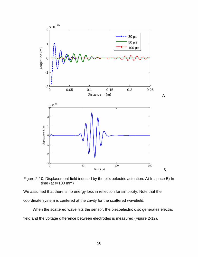
Eq.2-37 gives the response to each frequency component. Inverse FFT (iFFT) is
used to retrieve the time domain signal. The wave propagation in the plate is shown
with respect to the distance (Figure 2-10A) and time (Figure 2-10B).
The incident wave that reaches to the damage is described by fixing r=113.4 mm
in Eq.2-35. At r=113.4 mm, the displacement field changing in time can be described as
Figure 2-10B.
The third step is calculating the scattered wavefield. To analyze the scattering
behavior, we change our coordinate system centered at the cavity. Then, the incident
wavefield to the damage and the scattered wavefield from the damage are found using
Eq.2-9, 2.10 and Eq.2-13:
0
0
(2)
0
0
(2)
( 1) ( )cos
( , ) ( ) cos
( 1) '( )
( )
n
i n n
n
i t
s n n
n
n
n nn
n
u U J kr n
u r A H kr n e
U J kawhere A
H ka
(2-38)
The coefficients U0 are found by applying discrete Fourier transform to the signal
described by Figure 2-10B. Since this is an analytical expression for a single ω, we
apply FFT to the incident wave to transform the signal into frequency domain.
Accordingly, the coefficients An can be found from Eq.2-38, then we have the
frequency response. Then the result is transformed into time domain signal using iFFT,
and Figure 2-11 shows the scattered wavefield obtained at the sensor (r=113.4 mm).
50
0 0.05 0.1 0.15 0.2 0.25-2
-1
0
1
2x 10
-15
Distance, r (m)
Am
plit
ude (
m)
30 s
50 s
100 s
A
0 50 100 150-3
-2
-1
0
1
2
3x 10
-16
Time (s)
Dis
pla
cem
ent
(m)
B
Figure 2-10. Displacement field induced by the piezoelectric actuation. A) In space B) In time (at r=100 mm)
We assumed that there is no energy loss in reflection for simplicity. Note that the
coordinate system is centered at the cavity for the scattered wavefield.
When the scattered wave hits the sensor, the piezoelectric disc generates electric
field and the voltage difference between electrodes is measured (Figure 2-12).

51
0 50 100 150-1.5
-1
-0.5
0
0.5
1
1.5x 10
-17
Time (s)
Dis
pla
cem
ent
(m)
Figure 2-11. Scattered displacement response at r=113.4 mm from the cavity center.
0 50 100 150-5
-4
-3
-2
-1
0
1
2
3
4
5x 10
-4
Time (s)
Voltage (
V)
Figure 2-12. Electric signal obtained at the sensor position
Since the coefficients gij are given by the manufacturer, we can apply the sensing
equation (Eq.2-26) directly to obtain the voltage as shown in Eq.2.39.

52
1
31 31 313
11 11
1 2(1 ) (1 )
r r
E E
g d g u uE
s s r r
(2-39)
The displacement field ur is evaluated at r=113.4 mm, which is the position of the
sensor with respect to the cavity. Since we cannot assume an axisymmetric condition
for the sensing problem, this is a rough approximation of stress field within the
corresponding PZT sensor. Also, the PZT sensor is not small enough compared to the
wavelength (27mm), so there may be errors due to this approximation.
In Chapter 4, we have some experimental results for a damage detection problem
using PZT actuator and sensors. To verify this analytical solution, we compared the
generated voltage with experimental data that has identical configuration. Figure 2-13
shows the comparison between experimental signal and analytical solution.
0 50 100 150-3
-2
-1
0
1
2
3x 10
-3
Time (s)
Outp
ut
sig
nal (V
)
Experiment
Analytical sol.
Figure 2-13. Comparison with experimental data
The experimental data includes S0 mode and A0 mode simultaneously, and the
SNR (signal-to-noise ratio) is small because the scattered signal is weak. The
experimental signal has a SNR of three (4.7 dB, infinity norm). Also, the experiment

53
includes boundary reflections because it is not an infinite plate. However, if we
concentrate only the A0 mode, it is relatively easy to find the peak location and signal
shape corresponding to the experimental data.
Wavefield Simulation [51, 54]
Although the analytical solution is available for the structural wave propagation
problem, it is not always efficient to evaluate analytical solution. Since our damage
configurations are changing, we used a finite difference algorithm to simulate wave
propagation and scatter. This section introduces the finite difference algorithm we used,
which is developed in Matlab by Yuan et al. [51, 54]
Governing Equations of Flexural Waves
The governing equations of flexural waves are formulated, in this subsection, as a
first-order system that models the waves using a finite difference scheme, described in
the next subsection. Using the stress resultants (Qx, Qy, Mx, My, and Mxy) and the plate
displacement components (u, ψx, and ψy), the equations of motion can be written as:
2
2
23
2
23
2
12
12
yx
xyx xx
xy y y
y
QQ uq h
x y t
MM hQ
x y t
M M hQ
x y t
(2-40A)
and the constitutive equations:

54
12
2
2
1 0
1 0
0 0
x
x
y
y
xy
yx
x x
y y
xM
M Dy
M
y x
uQ Gh
x
uQ Gh
y
(2-40B)
In Eq.2-40, E and G are Young’s modulus and shear modulus respectively, q is
the transverse loading applied to the plate, h is the plate thickness, ν is the Poisson’s
ratio, ρ is the mass density, κ is a shear correction factor, κ2=π2/12, and
3 2/ [12(1 )]D Eh is the flexural rigidity. Substituting the plate stress resultants in
Eq.2-40B into Eq.2-40A, the equations of motions in terms of plate displacement
components can be obtained. Then, by eliminating ψx and ψy from the three motion
equations, a single differential equation in terms of transverse displacement u can be
written as:
2 3 2 2 2 2 2
2 2
2 2 2 21 ( , , )
' 12 ' 12 '
h u D hD u h q x y t
G t t t G h G t
(2-41)
where G' = κ2G. When the wave number is small and the thickness of the plate is
substantially smaller than the wavelength, Eq.2-41 can be approximated by
24
2( , , )
uD u h q x y t
t
(2-42)
Defining { , , , , , , , }T
x y y x x y xyu Q Q M M M u , { ,0,0,0,0,0,0,0}T qq and differentiating
Eq.2-40B, the result can be rewritten in the matrix form:

55
t x y
0 0 0 0
u u uE A B C u q
(2-43)
where
3
3
2
2
2 2
2 2
12
12
1
1
1
(1 ) (1 )
1
(1 ) (1 )
2(1 )
0 0 0 0 0 0 00 0 0 0 1 0 0 0
0 0 0 0 0 0 00 0 0 0 0 1 0 0
0 0 0 0 0 0 0 0 0 0 0 0 0 0 1
0 0 0 0 0 0 0 0 0 0 0 0 0 0 0
0 0 0 0 0 0 0 1 0 0 0 0 0 0 0
0 1 0 0 0 0 0 00 0 0 0 0 0
00 0 0 0 0 0
0 0 0 0 0 0 0
h
h
Gh
Gh
D D
D D
D
h
0 0E A
0 0 0 0 0 0 0
0 0 1 0 0 0 0 0
0 0 0 1 0 0 0 0 0 0 0 0 0 0 0 0
0 0 0 0 0 0 0 1 0 0 0 0 1 0 0 0
0 0 0 0 0 0 1 0 0 0 0 1 0 0 0 0
1 0 0 0 0 0 0 0 0 0 1 0 0 0 0 0
0 0 0 0 0 0 0 0 0 1 0 0 0 0 0 0
0 0 0 0 0 0 0 0 0 0 0 0 0 0 0 0
0 0 1 0 0 0 0 0 0 0 0 0 0 0 0 0
0 1 0 0 0 0 0 0 0 0 0 0 0
0 0B C
0 0 0
Finite Difference Algorithm
Based on the finite difference algorithm developed by MacCormack [50], a higher-
order algorithm is developed by Yuan [51, 54]. This algorithm is used in this study to
simulate the A0 reflection waves, which is programmed by Matlab. When the initial
condition at time step n is given by n n
0U E u, the output value of the next time step
Un+2 can be expressed using the MacCormack splitting method as
x y y xF F F F n+2 nU U
(2-44)

56
where Fx and Fy are the backward-forward operator in x- and y- direction, and Fx+ and
Fy+ are the forward-backward operator in x- and y- direction.
Although the explicit finite-difference scheme is computationally much more
efficient than the implicit scheme, it is restricted by CFL (Courant–Friedrichs–Lewy)
stability condition. CFL stability condition assumes that the waves are not allowed to
propagate over two grids in just a single time step, so that the properties of the waves
can be preserved in the numerical approximation and the stability is guaranteed. It
requires the numerical propagation speed Δx/Δt to be less than fastest wave
propagation wave. For the MacCormack scheme, the time step is limited by
max
2
3
xt
v
(2-45)
With vmax ≈ 3000m/s and Δx = 1.25 mm, the time step is chosen to be 0.2 µs.
Therefore, the total time of simulation is 250 µs with 1250 steps, which corresponds to a
5MHz sampling frequency in the experiment. For an aluminum plate which is 500 500
3.2t mm, the plate is discretized by a 400 400 rectangular grid, with grid spacing of
1.25 mm, and the excitation points is the center of the plate. A five-peaked tone burst
signal is emitted from the excitation grid and the wave signal is shown at each grid and
at each time step. Figure 2-14A shows a snapshot of the displacement field during
simulation at t=100 µs.
In the damaged plate simulation, the crack is modeled by altering the property
matrix E0 at the corresponding grid points. Figure 2-14B shows a snapshot of wave field
in the same plate with a 0.25 mm 0.125 mm rectangular hole (two grids), where we

57
can observe the scattered wave field. The domain is finite so boundary reflection is
present, but is much weaker than the visualized signal at t=100µs.
A B
Figure 2-14. A) Snapshot of the simulated structural wave propagating in the pristine plate at t=100µs. The toneburst wave is emitted from Actuator 4. B) Snapshot
of the wave in the damaged plate at t=100µs. The crack is 0.25 mm 0.125 mm and located at (-90, -110) mm from the origin.
The comparison between the numerical solution and the analytical solution is
presented in Figure 2-15. Since the numerical procedure does not model piezoelectric
effect, we only compare their shape and peak time. Also, there is a geometric
discrepancy between FDM and analytical solution due to limitation of representation in
FDM model. The geometry of damage is circular for the analytical solution, and
rectangular for the FDM simulation.
4

58
0 50 100 150-3
-2
-1
0
1
2
3x 10
-3
Time (s)
Sig
nal am
plit
ude
Analytical sol.
Finite difference
Figure 2-15. Finite difference solution compared with wave propagation analysis

59
CHAPTER 3 IDENTIFYING CRACK LOCATION USING MIGRATION TECHNIQUE
The objective of this chapter is finding the location of a crack using the migration
technique. The migration technique can identify and visualize the location of damage
from the sensor signals. This chapter discusses how we can visualize a crack within the
structure using the migration technique, and related topics to improve the performance.
Migration Technique
The concept of migration is that when a sensor receives a scattered signal, the
time of flight can be found by moving the signal in time domain and finding a time at
which the scattered signal matches best with the original excitation signal. In order to
find the best matching time, the cross-correlation concept is utilized. Cross-correlation is
a process to find the similarity of two correlated signals.
*( ) ( )( ) ( ) ( )
( )( )
(0) (0)
fg
fg
fg norm
ff gg
t f g t f g t d
tt
(3-1)
where f is the scattered wavefield at each sensor position, *fdenotes its complex
conjugate and g is the incident wavefield emitted from the actuator. t is the time
difference, and it defines the y-location of the intensity value. ( )fg normt
is the cross-
correlation coefficient.
Equation 3.1 indicates that if the two signals are identical, the correlation
coefficient (0)ff norm is 1, and if the two signals are completely out of phase (g= -f), the
coefficient (0)ff norm is -1. Here we find the similarity between excitation wave and

60
scattered wave by adjusting the time difference. Cross-correlation is often used to
compare two similar signals, and it is also known as temporal coherence [36]. The time
difference that gives maximum value of cross correlation coefficient is defined as the
time of flight (TOF).
Figure 3-1. Cross-correlation coefficient used to find the time difference between excitation and scattered signal in migration technique. c is the wave velocity
As shown in Figure 3-1, we find the similarity between excitation and scattered
signal. As we increase t to decrease the time difference between two signals, calculated
cross correlation coefficient increases when the last peak of excitation corresponds to
the first peak of scattered signal. It reaches the maximum value when all the peaks are
at the same position on the adjusted time axis, and decreases after that. Since the wave
velocity depends on material properties and frequency, the distance r is calculated from

61
the wave velocity and time difference.
One advantage of migration technique over other ultrasonic detection methods is
that the TOF is not a deterministic value, but is a range of possible values with
possibility specified by cross-correlation coefficient. This leaves a possibility to find the
best match between different pairs of actuators or sensors by comparing multiple
images.
Another advantage of using migration technique is that the damage image can be
readily obtained using the sensor to collect reflected waves from the damage. With the
image, the size and shape of the damage as well as its location can be quantified. That
is, more accurate and quantifiable damage profile using multiple actuator-sensor pairs
can be obtained. Image generation procedure will be discussed in detail later in this
section.
Figure 3-2. Actuator and sensor positions for migration technique

62
Although analytical solution to the wave propagation problem is available, wave
scatter cannot be described with a general formula. Instead, a finite difference algorithm
is used for simulation of migration technique. For simulation, an aluminum plate is
modeled to identify a through-the-thickness crack in the plate (Fig 3.2). The size of AL
6061 plate is 500 x 500 x 3.2(t) mm, and discretized by 200 x 200 equally spaced grids
(grid spacing: 2.5 mm). After the toneburst excitation is introduced, we examine the
response of the plate during 250μs with 1250 time steps. To illustrate the procedure, we
used signal information from every grid point along the sensor line, so that there are 200
equally spaced signal receivers along the line between 0 and 8. The crack is centered
at (-9, -11) cm from the center of the plate. The ultrasonic toneburst wave sent from the
actuator is a Hanning window modulated sinusoid transverse loading governed by:
2( ) ( ) 1 cos sin(2 )
p cc
c p
N f tq t P H t H t f t
f N
(3-2)
where P is the force, Np is the number of peaks of the loading, and fc is the central
(dominant) frequency. H is the Heaviside function, and Np =5, fc =110kHz, P=1N are
used for simulation. Because the PZT excitation is not modeled in the finite difference
scheme described in Section 2.4 due to scale difference, we directly apply loading q
instead of voltage to the central point.
The propagating and scattered wave is captured in the form of displacements at
each node. The migration technique uses Lamb wave propagation and reflection for
imaging damages in the structure. The location of excitation sources are shown in
Figure 3-2, and the actual force applied in time scale is shown in Figure 3-3. Sensor
locations where we measure the velocity are assumed to be at every grid for maximum

63
resolution.
0 10 20 30 40 50 60 70 80 90 100-1
-0.5
0
0.5
1
Time (s)
Forc
e (
N)
Figure 3-3. Excitation signal
We find the scattered wavefield by subtracting signal obtained from a healthy plate
from signal obtained from a damaged plate. By evaluating the scattered wavefield, we
can have the scattered wavefield in time and sensor position. Next step in migration
technique is back propagation. In time scale, we let the excitation wave to propagate
and do the cross-correlation to find the similarity between incident and scattered
wavefield. From those wavefields, image intensity is evaluated at every grid point. The
wave velocity multiplied by time difference t between excitation wave and scattered
wave indicates the distance from the sensor to the point we are evaluating. The cross-
correlation coefficient ( )fg normt
at the corresponding point is the image intensity in the
domain, and the higher image intensity becomes, the more likely to have damage at the
given location within the structure. The scattered wavefield f and incident wavefield g
are shown in Figure 3-4, and the detailed procedure is explained below.

64
A
B Figure 3-4. A) Scattered wavefield obtained at the sensor position (ordinate), B) Incident
wavefield for back propagation. Actuator is located at the origin
The cross-correlation coefficient is calculated for every individual sensor position,
which is the ordinate of Figure 3-4, and the time difference used in cross-correlation is
linearly related to the distance from the sensor since the velocity of A0 mode is constant
(3km/s). For example, the time difference between scattered signal and incident
wavefield at sensor position -100 mm (red line in Figure 3-4) is about 40 µs. Then the
cross-correlation coefficient is measured by Eq.3-1, and the image intensity value at the
position (-100, -120) mm from the center is assigned with the coefficient. So the

65
distance between sensor position and evaluating point is determined by multiplying the
time difference with the velocity of the incident wave, and the image intensity is the
cross-correlation coefficient. This procedure is done for every sensor position, and
every time difference.
Calculating the cross correlation coefficient requires a large amount of
computation for integration. To reduce the computation time, frequency domain
migration technique (f-k migration) was developed in geophysics [67-68] and extended
for SHM by Yuan et al [55]. F-k migration is computationally more efficient than the
reverse-time migration. The calculation speed is almost in real time. In f-k migration, the
signal is transformed to the frequency domain using discrete Fourier transform, and the
cross-correlation is calculated by Eq. 3.3
*( ) ( )( ) ( ) ( )
( )( )
(0) (0)
fg
fg
fg norm
ff gg
t f g t f g
tt
F F
(3-3)
Figure 3-5. Final images obtained by evaluating the image intensity at each point from simulation for a 50mm straight horizontal crack.

66
Figure 3-5 shows the case when the wave is simulated by FDM. Since we have
one image data from each excitation event, we have 7 images in total and prestack
approach developed by Yuan is used to obtain the final image [51].
So far, we have discussed how we can obtain images from signal using the
migration technique. As we have seen in the results, the images indicate damage
existence and its approximate location.
Bayesian Approach
Migration technique provides the inspector an image, which is easily interpreted
visually. However, the image only provides approximate location. Therefore, if we are
interested in more detailed information such as coordinates of cracks, we need to
improve its accuracy. From the images obtained from the migration technique, image
intensity refers to the grayscale value at each point in the images. This section
describes how to combine the image intensity of several images about one crack using
Bayesian approach.
Bayesian Approach
For more accurate estimation of crack location through migration technique, we
have applied Bayesian approach to the migration technique to enhance the result. The
main objective of this section is to improve the accuracy of detecting crack location by
using Bayesian update.
Bayes’ rule about conditional probability was suggested in the 1700’s, but the
development for practical applications has started in the 1900’s mainly because of the

67
computational burden. This rule is about conditional probability, and the rule consists of
simple formula stated in Eq.3-4.
( ) ( | )( | )
( )
P A l B AP A B
P B
(3-4)
This formula indicates that if we are interested in probability of A, given B, we can
calculate the probability by an inverse formula. P(A) is the prior probability of A, l(B|A) is
the probability of B, given A, which is called the likelihood, and P(B) is marginal
probability of B which acts as a normalizing constant. So this is especially useful when
we know the probability of B given A. Bayesian approach has been shown many times
to give better estimation by combining prior knowledge and likelihood to draw
conclusions [69].
The Bayesian framework can be applied to identify the location of the crack by
incorporating the image intensity data with prior information. When we have the image
intensity information, the coordinates of crack center can be stated by:
, ( , ) | ,, | ( , )
, ( , ) | ,
i
upd i
i
f x y l I x y x yf x y I x y
f x y l I x y x y dxdy
(3-5)
where x, y are the coordinates of a possible location of the center of the crack, ( , )iI x y
is the image intensity obtained from ith test, f is the prior distribution which is the current
state probability density that crack center exist at x, y without ith image intensity
information, and l is the likelihood function from current data, which is the probability
that we will get the image if the crack center is located at x, y.
In Bayesian approach, the likelihood function represents the relation between
actual crack center location and what we obtained. For this example, if the center of

68
crack is x, y then the probability density that we can obtain the image intensity from the
migration simulation is defined as the likelihood. In Eq.3-5, we assume that the image
intensity distribution along the x and y coordinates are independent, or the randomness
of the two is not correlated.
In this study, a horizontal crack centered at (-90, -110) mm with length of 40 mm is
considered. A five-peaked toneburst narrowband excitation with center frequency 110
kHz (duration of 44 μs) is emitted from an actuator. After the flexural waves propagate
in the plate, the reflected signals from the damage are detected by the sensors. Seven
actuators are excited sequentially and 200 sensors located along the x-axis collect
reflected waves for maximum resolution. Under this excitation frequency, only the first
fundamental flexural mode propagates in the plate. In an isotropic aluminum material,
the group velocity for the center frequency is around 3 km/s with wavelength of 27 mm.
We use finite difference method for calculating the wave propagation. An Al-6061
aluminum square plate with dimension 500mm × 500mm × 3.2mm is discretized by 200
× 200 plate elements. Simulated sensor data is collected from 1250 time steps (total
time span: 250 μs). Using the simulated sensor data, the migration technique is then
used for imaging the crack.
We start the process to determine the center of the crack location by assuming a
non-informative prior or initial distribution of x and y on the plate. Here we choose a
uniform distribution function as our prior distribution for plates that have never been
inspected before. Assuming that the origin is at the center of the plate, we can construct
a prior distribution as Eq.3-6, which implies that we have no information for the plate
before inspection and the damage might exist anywhere.

69
6, ( ; 250,250) ( ; 250,250) 4 10uniform uniformf x y f x f y (3-6)
where funiform is the probability density function of a uniform distribution. With the given
prior distribution, the next task is the selection of appropriate likelihood estimators
| ,il I x y for our next iteration. In this case, the test result iI indicated by the image
intensity is a deterministic known value obtained in the simulation. If the center of crack
is x, y then the probability density that we can obtain the image intensity from the
migration simulation is the likelihood.
However, due to computational cost of the migration techniques, accurate
estimation of likelihood estimator is almost impossible. Instead, we suggest several
ways to assume and estimate l through error analysis. In the following two subsections,
we suggest two basic ways to construct the likelihood estimators, direct image intensity
and multivariate normal distribution.
Direct Image Intensity
The simplest way to construct a likelihood function out of given image is direct
interpretation of the given image intensity to our likelihood function. In other words, the
probability that we will get the image when the center of the crack is at point (x, y) is
proportional to the image intensity at (x, y). In this case the likelihood estimator is
defined by Eq.3-7.
( | , ) ( , )i il I x y I x y (3-7)
Using this likelihood function with Bayesian updating with all seven images from
the seven actuators, we obtained the final distribution shown as an image in Figure 3-6.

70
A B
C
Figure 3-6. Combining image using direct image intensity as likelihood A) Up to 3rd actuator B) Up to 5th actuator C) Up to 7th actuator (final)
Multivariate Normal Model about Center of Intensity
Instead of using the entire image data, we may elect to use only the center of
intensity to estimate where the center of the crack is. The center of intensity of an image
obtained from ith actuator is defined by Eq.3-8.
, ,
( , ) ( , ),
( , ) ( , )
i i
c i c ii i
xI x y dxdy yI x y dxdyx y
I x y dxdy I x y dxdy
(3-8)

71
This estimation has errors associated with the migration technique. By simulating a
large number of cracks, we found that the error in estimated location from each actuator
follows a simple trend defined by a bi-variate normal distribution, and the variation due
to location of crack center is observed (Figure 3-7).
A B
-5 -4 -3 -2 -1 0 1 2 3 4
0.003
0.01
0.02
0.05
0.10
0.25
0.50
0.75
0.90
0.95
0.98
0.99
0.997
Error in x- direction
Pro
babili
ty
Normal Probability Plot
C-1 -0.5 0 0.5 1
0.003
0.01
0.02
0.05
0.10
0.25
0.50
0.75
0.90
0.95
0.98
0.99
0.997
Error in y- direction
Pro
babili
ty
Normal Probability Plot
D
Figure 3-7. Estimation error in x and y directions. We tested 117 different crack configurations with different actuators and calculated the difference between actual locations and the estimated locations. A and B shows estimation error associated with location of crack center, and C and D shows normal fit of the error distribution.
So, we defined a multivariate normal model for the likelihood in Eq.3-9.
, ,
2 2
, 1 ,
| , | |
ˆ( ; , ) ( ; , )
i i i
c i c i
normal c i x normal c i y
l I x y l x from I x l y from I y
f x x c x f y y y
(3-9)

72
where the parameters are estimated as 24.2 , 6.0x ymm mm , and linear coefficient
in x direction as 1 1.62c from Figure 3-7A and the bias in y direction as ˆ 3.07y mm
from Figure 3-7D.
The bi-variate distribution gives the probability of the center of intensity being at a
point, given that the center of the crack is at (x, y). Using Bayesan updating with this
likelihood function with all seven images from seven actuators, we obtained the final
distribution shown as an image in Figure 3-8. The estimated locations by center of
intensity and their error in the crack center location are shown in Table 3-1.
A B
C Figure 3-8. Combined image using multivariate normal model. A) Up to 3rd actuator B)
Up to 5th actuator C) Up to 7th actuator (final)

73
Table 3-1. Estimation error due to different imaging techniques
Likelihood estimators Estimated location (mm)
Distance from true crack center (mm)
Actual -90.0, -110.0 -
Prestack migration -81.1, -104.0 10.73 Direct image intensity -82.7, -105.7 8.47 Multivariate normal -91.4, -105.5 4.71
Table 3-1 shows that the estimated crack center is closer to the true crack center.
Although the improvement is small, we have much more focused images such as Figure
3-6 and Figure 3-8 compared to prestack images shown in Figure 3-5. So the chance of
misinterpretation of crack location is low.
Compensation for Geometrical Decay
In the previous section, we have introduced a Bayesian approach to improve the
accuracy of crack center location by images obtained from the migration technique.
However, it is found that there exists a bias of the detected damage location due to
different sensor-actuator combinations. We have concluded that the bias came from
geometrical decay. As a result, the image intensity when the damage is located close to
the actuator and sensors is higher with the image when it is located far from the
actuators and sensors. This happens because the image intensity depends on the
distance from the sensor and actuator. To compensate the effect of distance on image
intensity and to obtain a more accurate location of the damage, a correction method for
signal decay is suggested.
For 2D or 3D structures, the strength of propagating Lamb wave experiences
geographical decay caused by dispersion of wave to larger wavefront at a longer
distance region. In addition, the white noise in the signal is greatly amplified near the

74
actuator. As a result, the image intensity in the sensor shows a combined effect of
reflection and distance from damage. The signal amplitude differs a lot when we have a
crack at a different location. To summarize, the signal amplitude for small damages that
are close to the sensor and actuator is larger than that of large or severe damages that
are far from the sensor and actuator (Figure 3-9).
A
B
Figure 3-9. Possible errors related to geometrical decay A) The estimated center of damage may have an error B) Damages that have the same size are depicted differently because of their locations.
The idea of compensating for decay of signal such as attenuation was first
proposed in the medical imaging area [66]. When ultrasonic waves are used for medical
imaging, the effect of decay causes many problems, and more accurate images are

75
obtained by compensating for attenuation of signals. In this section, the compensation
procedure is introduced to SHM in order to solve the inaccuracy problem and to
decompose the size from location simultaneously.
Geometrical Decay in Plate Wave
As described in Chapter 2, when an ultrasonic pulse disperses from a point
source, the amplitude experiences a decay described by Bessel function in space, and
experiences exponential decay in time. From the asymptotic function of Bessel function,
the maximum amplitude A at distance r can be described as:
1 1A
kr t
(3-10)
where k is the wave number.
In the actual simulation and experiment, a five-peaked tone-burst signal is used for
successful generation of Lamb waves within the plate. However, the initial amplitude
does not follow the above relation closely because of the transient response and inertia
effect. By using finite difference simulation, the geometrical decay of signal with respect
to time and distance is calculated, as shown in Figure 3-10A. We used 200 x 200 grids
in an Al 6061 square plate of 500 x 500 x 3.2 mm to simulate the results.
Also, we have obtained the profile of decay of the maximum amplitude as a
function of time (Figure 3-10B). The graph fits Eq. 3.10 well after all the transient effects
are gone. Figure 3-10B shows the maximum amplitude specified from simulation at
each time step. As time goes by, and the wave travels further, the signal strength
decreases due to dispersion. Thus, the signal strength highly depends on the location of
the damage as well as its severity. In the imaging technique, this causes weak signal in
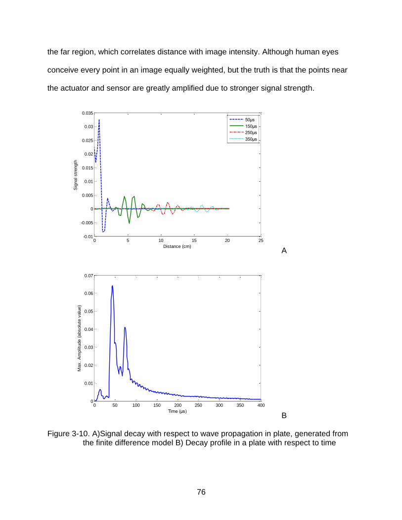
76
the far region, which correlates distance with image intensity. Although human eyes
conceive every point in an image equally weighted, but the truth is that the points near
the actuator and sensor are greatly amplified due to stronger signal strength.
0 5 10 15 20 25-0.01
-0.005
0
0.005
0.01
0.015
0.02
0.025
0.03
0.035
Distance (cm)
Sig
nal str
ength
50μs
150μs
250μs
350μs
A
0 50 100 150 200 250 300 350 4000
0.01
0.02
0.03
0.04
0.05
0.06
0.07
Time (μs)
Max.
Am
plitu
de (
absolu
te v
alu
e)
B
Figure 3-10. A)Signal decay with respect to wave propagation in plate, generated from the finite difference model B) Decay profile in a plate with respect to time

77
From the observations made in the simulation, a compensation curve is
constructed using a Matlab curve fitting tool (cftool). We assumed that the amplitude A
is inversely proportional to time t following this relation:
1/ ( ) ( )
1 ( , )
d d
d
t t t tA
t t unknown
(3-11)
where td is a threshold time for the transient region. We assume that the amplitude is
uniform during the transient period. From data analysis, we choose td = 58 μs.
There are two ways to compensate for attenuation of signal strength. One is to
apply the compensation scheme in the time domain, while the other is to apply it in the
spatial coordinates. In this section, we construct the curve in Eq.3-11 based on time
domain and applied to the received signal directly (Figure 3-11). After that, the back
propagation stage of migration technique is compensated based on distance.
Compensating for back propagation stage is discussed in the next section.
0 200 400 600 800 1000 1200 1400-5
0
5x 10
-5
Time
Am
plit
ude
Original
Compensated
Figure 3-11. An example of compensated signal displayed on time scale.
Application to Migration Technique
The migration technique comprises two different steps: detection of the reflected
wave and back-propagation. Then the image intensity is calculated by cross-correlation
of the reflected wave and the back-propagated wave. The reflected wave first travels

78
from the actuator to damaged site and as the wave hits the damage, the reflective wave
propagates as if the source is at the point of damage. During these propagation paths,
the wave strength decays.
Then the back-propagated wave also decays when traveling the distance between
actuator and a point. By calculating the cross-correlation, or convolution, of these two
waves, the image intensity I has a relation stated in Eq. 3.12, and the compensated
image intensity can be calculated by Eq.3-13.
2 2
actuated reflected actuator-distance sensor-distance1/I A A d d (3-12)
2
d corr actuator distance sensor distanceI Id d (3-13)
where I is the image intensity used to represent the possible damage location in the
domain, A is the amplitude of a signal, and d is the distance between the
actuator/sensor and the point in the domain.
We applied the signal compensation, and in addition to that, corrected image
intensity is calculated by 2
actuator-distance sensor-distanceId d at a point (x, y). With this procedure, the
effect of distance from the imaging result is eliminated.
Numerical Simulation
The simulation is done by finite difference scheme using 200 x 200 grids on a 50 x
50 x 0.32 cm square plate with 1250 time steps (1μs time interval). A straight, horizontal
crack is centered at (-9, -11) cm from the center of the plate, and the size is 4 cm.
Those three techniques use the same sensor information.
Figure 3-12 shows the images obtained from the three methods, using the
migration technique, using Bayesian approach (Section 3.2), and applying

79
compensation for geometrical decay in addition to Bayesian approach. The three
images do not show a significant difference about the location at a glance, but the error
of estimation of crack center location is greatly reduced by attenuation compensation.
The crack center location is obtained from taking the mean of entire image. Table 3-2
summarizes the results.
A B
C Figure 3-12. Images from migration technique with the same sensor data. A) Prestack
approach B) Bayesian approach C) Bayesian approach with compensation for geometrical decay
Also, in order to check if the formula for compensation is valid, we also simulated
several crack locations to check if they yield a consistent level of image intensity with
respect to size. The result is shown in Figure 3-13 and Table 3-3.

80
Table 3-2. Comparison of accuracy, different imaging results.
Imaging method Estimated location (mm) Distance from true crack center (mm)
Actual -90.0, -110.0 -
Prestack migration -81.1, -104.0 10.73 Bayesian approach -82.7, -105.7 8.47 Bayesian approach with compensation factor
-88.6, -108.3 2.20
Figure 3-13. Image intensity distribution for a single actuator image
Table 3-3. Comparison of imaging results
Crack location Estimated location (cm) Difference (cm) Max. Intensity
(-7, -15) cm (-6.63, -14.65) cm 0.509 cm 1.047 x 10⁻¹¹
(-12, -3) cm (-13.02, -3.17) cm 1.034 cm 4.998 x 10⁻¹²
In principle, all images of a crack regardless of the actuator location should
provide the same value of image intensity after compensation. However, we observed
that the image intensity of a closer actuator is still greater than the others. This is
because that the crack orientation, reflection angle and other minor characteristics are
not fully considered in the compensation procedure. We did not include them in the
procedure since they only have a minor effect, and they tend to be easily contaminated
by the error in real situation.

81
We have applied the idea to Migration technique to improve it with compensation.
The numerical results showed an improvement of accuracy of the estimated crack
center location. In SHM, many diagnostic techniques using ultrasonic wave propagation
and reflection have been suggested. There are techniques that reduce location error by
time of arrival, but it is not sufficient enough for decomposing the effect of signal
strength and distance. The location from the image obtained from diagnosis mainly
depends on the time of arrival, but the effect of signal strength still remains in the image.
In a previous study on the migration technique, our research group has discovered the
biased error due to this feature [57]. In order to compensate for the bias error of
detecting crack location, we suggested a compensation for decay of signal strength for
ultrasonic imaging techniques. The motivation for this application is improving numerical
accuracy of detection techniques suitable for transfer to prognostic stage. Since the
prognosis process involves a large amount of uncertainty compared to diagnosis, a
small error may be critical for evaluating remaining lifecycle of the structure.

82
CHAPTER 4 EXPERIMENTAL STUDY ON IDENTIFYING CRACKS OF INCREASING SIZE
An experiment is conducted to explore the relationship between the sensor signal
amplitude and crack size through experiments and simulation for estimating the size.
The objective of this chapter is to explore the relationship between the sensor signal
amplitude and crack size through experiments and simulation for estimating the size.
Cracks are machined into an aluminum plate with increasing size, and measurements
are carried out with ultrasound excitation using piezoelectric transducer arrays that
alternate their role as actuators or sensors.
Test Panel and Test Procedure
An Aluminum 6061 panel (600mm×600mm×3.2mm) was tested for examining the
ability to estimate the size of a through-the-thickness crack. Table 4-1 shows the
mechanical properties of the panel. In order to detect a crack, we used two sets of linear
sensor/actuator arrays, with each set containing nine lead zirconate titanate (PZT) discs
(diameter 10 mm; thickness 0.4 mm, refer to Table 4-2). Each PZT disc can be a sensor
or an actuator. The equally-spaced sensor arrays are attached to the plate by epoxy
bond (Loctite 401) as shown in Figure 4-1C with 62.5 mm spacing, and the total length
of sensor array is 500 mm. The two sets of linear arrays are used to study the effect of
crack location. Figure 4-1C also shows a vertical array of sensors, which is not used for
this paper. When a PZT disc is used as an actuator, all other PZT discs in the array are
used as sensors. The sensors at both ends (numbered 0 and 8) are not used as
actuators but only as sensors. Thus only seven PZTs are used as actuators to emit the
ultrasonic signal into the plate, and the Lamb wave generated from the actuator is

83
recorded at the remaining sensors for both the pristine and damaged states for every
crack increment. The excitation from the PZT is a five-peaked toneburst signal.
Scattered wavefield from the damage is calculated by the difference between the
pristine and damaged states. The crack was manufactured first by drilling a 4.5mm
diameter hole centered at (-90mm, -110mm) at the center of the plate. Afterwards, we
gradually increased the size of the damage to form a shape close to a straight crack up
to 50 mm in length by machining (Figure 4-2). The fifteen crack sizes tested are listed in
Table 4-3.
Table 4-1. Mechanical properties of aluminum plate
Young’s modulus E (GPa) 72 Poisson’s ratio ν 0.3 Density ρ (kg/m3) 2.73 × 10³
Table 4-2. Properties of piezoelectric disc (modified PZT-4)
Geometry (mm) diameter:10.0, thickness:0.4 Density ρ (kg/m3) 7.9 × 10³ Young’s modulus E (GPa) E11: 86, E33: 73 piezoelectric coefficient d31 (m/V) -140 × 10-12 Piezoelectric coefficient d33 (m/V) 320 × 10-12 Piezoelectric coefficient g31 (Vm/N) -11 × 10-3 Piezoelectric coefficient g33 (Vm/N) 25 × 10-3 Dielectric constant K3 1400
Table 4-3. List of crack sizes tested, (unit: mm)
2.5 (hole) 13.8 31.5 3 (hole) 16 35 4.5 (hole) 18 40 9 21 45 11 26 50
NI PXI-1000B system was used for data collection with the LabView program. The
sampling rate was set to 5MHz, and the signal resolution was 16-bit. Since the resulting
signal amplitude from the sensors was very small, a Piezo Linear Amplifier EPA 104

84
A B
C
Figure 4-1. Layout of actuators and sensors A) One set of sensors for simulation and experiment B) Two sensor arrays attached to the plate and their corresponding domain C) Aluminum 6061 test plate – pristine state. Three arrays of sensors are attached to the plate, but the vertical array is not employed in this research.
A B
Figure 4-2. Damage manufactured to the plate A) 16 mm damage centered at -90, -110 mm B) 50 mm machined crack
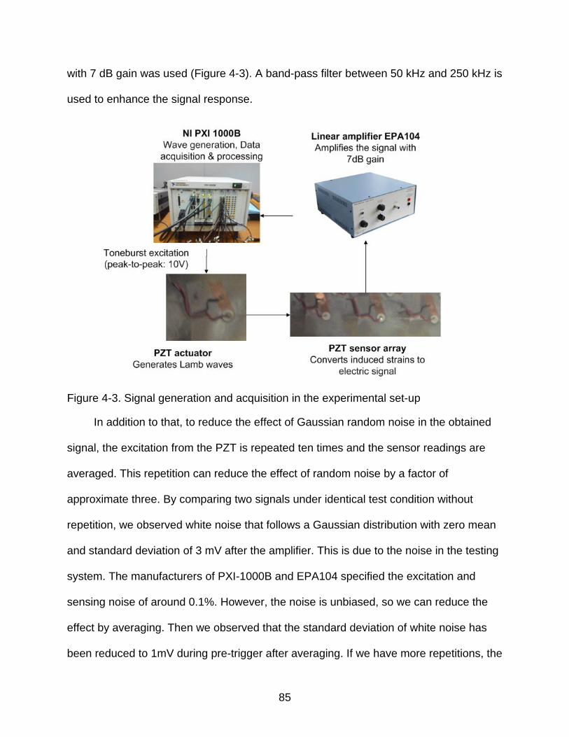
85
with 7 dB gain was used (Figure 4-3). A band-pass filter between 50 kHz and 250 kHz is
used to enhance the signal response.
Figure 4-3. Signal generation and acquisition in the experimental set-up
In addition to that, to reduce the effect of Gaussian random noise in the obtained
signal, the excitation from the PZT is repeated ten times and the sensor readings are
averaged. This repetition can reduce the effect of random noise by a factor of
approximate three. By comparing two signals under identical test condition without
repetition, we observed white noise that follows a Gaussian distribution with zero mean
and standard deviation of 3 mV after the amplifier. This is due to the noise in the testing
system. The manufacturers of PXI-1000B and EPA104 specified the excitation and
sensing noise of around 0.1%. However, the noise is unbiased, so we can reduce the
effect by averaging. Then we observed that the standard deviation of white noise has
been reduced to 1mV during pre-trigger after averaging. If we have more repetitions, the

86
white Gaussian noise can be further eliminated, but we limited ourselves to only 10
repetitions because only 10 repetitions can have a SNR (infinity norm) of three for the
smallest damage.
Figure 4-4. Test procedure for estimated location by migration technique and signal amplitude measurement
The scattered wavefield from the crack was obtained by subtracting the pristine
plate signal from the signal from the damaged plate (Figure 4-4). Then, the maximum

87
peak-to-peak amplitude of the scattered signal was identified. In addition, the migration
technique was used to create an image of the damage for an approximate location of
the crack.
To determine the excitation frequency, a preliminary experiment was performed
using an identical plate prior to actual testing. By using two piezoelectric transducers
attached on the same location on the plate, but opposite sides through the thickness
and a PZT sensor on the different location, we examined the amplitude difference due
to different excitation frequencies. Because of the low value of the product of frequency
and plate thickness, only the fundamental modes of symmetric and anti-symmetric
waves, also known as S0 and A0 modes propagate in the plate.
50 100 150 200 2500
0.1
0.2
0.3
0.4
Frequency(kHz)
Am
plit
ude (
V)
S0mode
A0mode
A0 20 40 60 80 100
-10
-5
0
5
10
Time (s)
Sig
nal (V
)
B
Figure 4-5. A) Frequency sweep experiment. Amplitudes of transmitted signal are shown for A0 mode and S0 mode. B) Five peaked toneburst excitation sent to the actuator (110 kHz)
In this study, only the A0 mode was used to examine the scattered signal since it
has larger amplitude than S0 mode at the frequency of interest and is highly dispersive.
The central frequency was chosen to be 110 kHz corresponding to the wavelength
27mm based on the result of this frequency-amplitude experiment, which gives the
maximum amplitude of A0 mode excitation (Figure 4-5A). The five-peaked toneburst
used for wave excitation is shown in Figure 4-5B.

88
Results
Scattered Signal from the Damage
In simulation, the transverse velocity is chosen as the sensing parameter at the
corresponding nodes, and the maximum amplitude is proportional to the maximum
strain or voltage at each piezoelectric transducer disc in the experiment. In both
simulation and experiment, the scattered signal is obtained by subtracting the pristine
plate signal from the damaged plate signal. Figure 4-6 displays a sample case when the
crack size is 26 mm and the excitation point is at Actuator 4, which is located at the
center of the plate (Figure 4-1).
In Figure 4-6, symmetry between left and right sides of actuator 4 was expected
and observed in the simulation, but the experiment showed substantial asymmetry. This
is attributed to differences in individual sensor quality and attachment uniformity.
However, we have observed reasonable agreement between simulation and experiment
in terms of time of flight (TOF) and scattered signal amplitude.
Variation of the Signal with Crack Size
Maximum peak-to-peak amplitude of a signal represents the maximum strain
energy transfer rate by the given signal. By examining the maximum peak-to-peak
amplitude of the scattered signal, we can observe that the amplitude increases with
crack size. Figure 4-7 shows the change in the scattered signal amplitude for two
different crack sizes.
We have seven excitation sources, and for each excitation, eight sensors are used
to examine the scattered signal. The highest peak-to-peak amplitude among all sensors
and actuators is the maximum signal amplitude for each crack size. The maximum

89
Figure 4-6. Toneburst excitation measured from all eight sensors from simulation (a, b, c) and experiment (d, e, f). Sensor spacing is 62.5 mm each. (a) pristine plate signal (b) damaged plate signal (c) scattered signal by subtracting (a) from (b). We can observe the scattered signal from the boundaries in experiment, but it is almost completely removed after subtraction. (d) pristine plate (e) damaged plate (f) scattered signal by subtracting (a) from (b) (Signal amplitude is adjusted for (c) and (f) because the scattered signal is much smaller than the healthy or damaged ones)

90
0 50 100 150-0.08
-0.06
-0.04
-0.02
0
0.02
0.04
0.06
0.08
Time (s)
Sig
nal am
plit
ude (
V)
0 50 100 150-0.08
-0.06
-0.04
-0.02
0
0.02
0.04
0.06
0.08
Time (s)
Sig
nal am
plit
ude (
V)
Scattered signal
from a 9mm crackScattered signal
from a 31.5mm crack
Figure 4-7. Experimental scattered signal amplitude change in different size cracks. A) 9 mm B) 31.5 mm
amplitude occurred usually at actuator 3 and sensor 2 for all crack sizes, except that for
cracks sizes 2.5mm, 3mm, and 4.5mm it happened at actuator 4 and sensor 2. Due to
difficulty in modeling the actuator and sensor interaction with the plate, normalized
measured signals are compared to normalized signal velocities. Without loss of
generality, the data are normalized with respect to the signal amplitude when the crack
size is 25 mm. The comparison between normalized values of signal amplitude is
presented in Figure 4-8. It can be seen that the relation is proportional to the crack size
of 30 mm, and showed a good agreement between experiment and simulation.
The major observation in this experiment is that the signal amplitude increases
with crack size up to a saturation point. This provides us a capability to monitor a crack
growth up to a certain size.
A0
A0 S0
S0

91
0 10 20 30 40 500
0.5
1
1.5
2
Norm
aliz
ed s
ignal am
plit
ude
Crack size (mm)
Experiment,
excitation 110kHz
Simulation,
excitation 110kHz
Figure 4-8. Signal amplitude variation (maximum peak-to-peak amplitude). The excitation frequency is 110 kHz and the signal amplitude is normalized using the signal at crack size 25 mm as the reference.
Effect of Frequency
Figure 4-8 shows divergence of signal amplitudes between measurement and
simulation when the crack size is longer than 30mm. To investigate this further, the
experiment was repeated using a different excitation frequency. Since the signal from
the experiment has both S0 and A0 mode, we examined individual signal to determine
which is dominant. This is possible because S0 mode is significantly faster than A0
mode (Figures 4-7 and 4-9).
While the signal amplitude of S0 and A0 mode has similar magnitude for this
central frequency, we observed that A0 mode amplitude is still larger than S0 mode in
the scattered signal (Figure 4-9).

92
0 50 100 150-0.08
-0.06
-0.04
-0.02
0
0.02
0.04
0.06
0.08
Time (s)
Sig
nal am
plit
ude (
V)
Scattered signal
from a 31.5 mm
crack 150kHz
Figure 4-9. Scattered signal amplitude with 150kHz excitation.
The result, obtained at the same crack sizes with a different central frequency of
150 kHz, is presented in Figure 4-10. The amplitudes are normalized by the same scale
factor as the previous result. In this case, the agreement between experiment and
simulation was maintained up to crack size of 22 mm.
This time the separation between the two graphs occurs around 22mm. We
speculate that is related to the wavelength (150 kHz, A0 mode wavelength λ≈20 mm,
and 110 kHz, λ≈27 mm). Since all other conditions are identical and the group velocity
of A0 mode propagation in the plate is almost the same for both frequencies, we
concluded that the agreement may deteriorate for crack sizes larger than the
wavelength. Since we have fixed excitation frequency, the crack size is a linear function
of Helmholtz number. So we can also say that the scattered signal will change as a
function of the Helmholtz number.
S0
A0

93
0 10 20 30 40 500
0.5
1
1.5
Crack size (mm)
Norm
aliz
ed s
ignal am
plit
ude
Experiment,
excitation 150kHz
Simulation,
excitation 150kHz
Figure 4-10. Signal amplitude variation (maximum peak-to-peak amplitude). The excitation frequency is 150 kHz and the signal amplitude is normalized using the same scale factor as Figure 4-8.
It is known that if Helmholtz number (the ratio of the crack size to the acoustic
wavelength) is large, there is cutoff frequency where we cannot observe the increasing
signal amplitude. The Helmholtz number for 110 kHz excitation to examine 30 mm crack
is 1.11, and for 150 kHz excitation to examine 22 mm crack is 1.10. Theoretically, the
cutoff Helmholtz number is 1.84 for a circular cavity which is of the same order of
magnitude as our observation, so we concluded that as the Helmholtz number
approaches its cutoff point, deviation between simulation and experiment begins to
increase.
Also, the signal amplitude behavior beyond this point may be due to geometrical
discrepancies; for example, the crack tested in the experiment is not perfectly straight.
For longer cracks, the geometric variations are responsible for the change in the
maximum amplitude by changing the amplitude along the directions of scattered waves.

94
In other words, we require more precise modeling for better agreement between
simulation and experiment. The main reason that we do not discuss further on this
effect is that we still can cover a wider range by changing the excitation frequency.
However, when we are interested in long cracks, we can estimate the size by
processing images obtained from migration technique or other techniques for general
crack shapes. 11 mm crack also showed an abnormal result, but it is probably due to
the transition from a circular hole to a hole plus a machined crack around that size.
Crack Location Effect
We next investigated the effect of the relative location of the crack and the sensor
array. Figure 4-11A shows two sensor arrays on a single plate and the simulation
domain covered by each array. The crack is located at (-90mm, -110mm) from sensor 4
of array 1, while it is located at (-100mm, -140mm) from sensor 4 of array 2. The
experiment for two different domains is essentially equivalent to cases for two different
crack locations (Figure 4-11B). The behavior of maximum signal amplitude is predicted
by simulation, and obtained from experiment. By using sensor array 2, we were able to
obtain the signal amplitude for crack position 2, and compared it with the simulation
results in Figure 4-12.
Since the distance from the sensor array is larger, the slope of peak-to-peak
amplitude to the crack size is smaller compared to the previous experiment, but slightly
larger than expected from the simulation. The sensors have some variability, so the
sensors used later might be more sensitive than the one used in Figure 4-8. Therefore,

95
A -300 -200 -100 0 100 200 300
-300
-200
-100
0
100
200
300
position (mm)
positio
n(m
m)
Crack position 1 (-90,-110)mm
Crack position 2(-100,-140)mm
PZT actuator/sensor positions
B
Figure 4-11. A) Two sets of sensors and the domains covered by each array B) Different crack center location with respect to the actuator positions: second crack center location is (-100mm, -140mm)
0 10 20 30 40 500
0.2
0.4
0.6
0.8
1
1.2
1.4
1.6
Crack size (mm)
Norm
aliz
ed s
ignal am
plit
ude
Experiment, position1
Experiment, position2
Simulation, position2
Simulation, position1
Figure 4-12. Scattered signal amplitude variation for cracks growing at a different location excited by 110 kHz ultrasonic toneburst. Signal amplitude comparison with result shown in Figure 4-8, simulation and experiment.

96
a different crack location as well as the sensors require a different calibration factor,
which represents a different slope between crack size and signal amplitude. In our case,
the factor is not calculated but we have performed another simulation to find more
accurate relation. With the updated predicted behavior, we were able to find a linear
relationship between signal amplitude and the crack size for the second location.
Since approximate crack location may be found by the migration technique, the
calibration factor, or the coefficient for the linear relation, can also be found from that
information. However, uncertainty in individual sensor characteristics and estimated
location may be encountered during the procedure. To implement an SHM system to
real-life structures, more research has to be done to overcome these difficulties.
Migration Technique with Experimental Data
Chapter 3 discussed how we can identify crack location using simulated signal.
With the same procedure, we can obtain images using experimental signal. In this case,
we only have a limited number of sensors, so the scattered wavefield is reconstructed
from the sensor signals by spline interpolation (Figure 4-13).
Figure 4-14 and 4-15 shows experimental results. Figure 4-14 shows the image
obtained from one actuator and nine sensors. The final result is obtained by combining
images in Figure 4-15 and Table 4-4.
Table 4-4. Comparison of different imaging methods
Imaging method Estimated location (mm) Error (mm)
Actual -90.0, -110.0 - Prestack migration N/A Bayesian approach -95.5, -104.0 8.14 Bayesian approach with signal decay compensation
-90.8, -106.2 3.88

97
Figure 4-13. Reconstructed scattered wavefield
Figure 4-14. Experimental result is reproduced into image using migration technique. The crack size is 50 mm, and actuator position is at the center of the plate.

98
A
B
C Figure 4-15. Combination of all 7 actuators available in the experiment. The crack size
is 50mm. A) Prestack approach B) Bayesian approach C) Bayesian approach with signal decay compensation

99
Figure 4-15A uses migration technique described in Section 3.1. The image clearly
indicates that there is damage, but the location is inconclusive. Figure 4-15B utilized the
Bayesian approach suggested in Section 3.2, and we have a focused image where we
can extract the coordinates of crack center. Figure 4-15C applied signal decay
compensation (Section 3.3) on top of Bayesian approach (Section 3.2), and the
estimated location is closer to the true crack center.

100
CHAPTER 5 BAYESIAN APPROACH TO IMPROVE DIAGNOSIS FROM PAST PROGNOSIS
The goal of this chapter is to improve size estimation accuracy by taking
advantage of previous prognosis. First, it is acknowledged that the measured crack size
from SHM systems may have error and noise, which can be represented using a
statistical distribution. With a series of inspection results available, we can make a
prediction about how the crack will grow by the next inspection cycle using several
methods. This can help narrow down the uncertainties involved in diagnosis by applying
our knowledge from previous prediction of crack propagation. The procedure introduced
in this chapter is very similar to the particle filtering approach [77, 78]. However, one
difference is that the particle filtering generates crack size candidates and updates their
weights for the next prior distribution, while this approach directly calculates the prior
distribution using Monte Carlo Simulation.
Section 5.1 presents the crack propagation problem for fuselage panels, and
Section 5.2 explains how to perform a Bayesian approach to take advantage of past
prognosis. Section 5.3 presents the simulation results.
Modeling
The fuselage is the main structure or body of the aircraft to which all other units
attach. It provides space for the crew, passengers, cargo, most of the accessories, and
other equipment (Figure 5-1). Typically, many panels are assembled together in the
fuselage. However, when the airplane is under operation, it is subjected to a cyclic
fatigue loading due to repeated pressurization. As a result, the number of cycles
corresponds to the number of flights. Problem formulation for this low-cycle, high stress

101
fatigue is simplified by an infinite plane with uniform loading in one-direction (Figure 5-
2).
Figure 5-1. Aircraft fuselage
2a
σ
σ
Figure 5-2. Simplified loading condition
A through-the-thickness center crack in a fuselage panel is considered. Since the
pressurization is the major loading factor for a fuselage, the crack propagation can be
considered as a low-cycle fatigue. Paris’ law is used to model the true crack behavior
during the simulation (Eq. 5.1).

102
m
I
daC K
dN
(5-1)
where a is the half crack size, N is the number of loading cycles (treated as a real
number), K a is the range of stress intensity factor, Δσ is the difference
between maximum and minimum applied stress, and C and m are crack propagation
parameters related to material properties and geometry.
We also assume that the material has inherent defects, or micro cracks within the
structure where the crack starts growing from them. With the parameters given in Table
5-1, the true crack propagation is modeled by the solution of the Paris’ law as shown in
Eq.5-2 and Figure 5-3. Note that the crack size a(N) shown in Eq.5-2 is a half crack
size.
2
212( ) (1 )( )
2
m mm
i
ma N NC a
(5-2)
Table 5-1. Parameters related to simulated crack propagation.
Parameters Value
Initial flaw size, ai 1 mm
Minimum detectable crack size 6 mm Maximum allowable crack size 50 mm Crack propagation parameter, C 2.0 × 10⁻¹⁰ Crack propagation parameter, m 3.7 Applied stress Δσ 78.63 MPa SHM Inspection interval 50 cycles First detection 34,300 cycles Total life 42,300 cycles
The minimum detectable crack size of SHM is larger than that of manual
inspection. In ultrasonic testing, the minimum size is about a half of the wavelength of
the excitation wave [5]. Since there are practical limitations of the excitation frequency

103
0 0.5 1 1.5 2 2.5 3 3.5 4 4.5
x 104
0
10
20
30
40
50
N (cycles)
Cra
ck s
ize (
mm
)
First detection
Figure 5-3. Crack propagation. We assumed that the crack is first detected when it is
bigger than 6mm.
that we can use, the minimum detectable crack size that we can use is around 5 ~ 10
mm. Therefore, we assumed that the minimum detectable crack size to be 6 mm for this
research. After the detection returns a positive signal, the crack will be monitored until it
is sent for maintenance, which is defined to be 50 mm in crack size. In this research, the
probability of detection is not considered.
Uncertainty in the detected crack size varies widely by inspection methods, data
processing techniques, and associated noise with the procedure. In this research, we
consider the uncertainty induced by white noise in the signal, which is unbiased. In
general, it is known that the uncertainty of the detected size is larger when the crack is
large [35,72], so this chapter models the ratio between true crack size and inspected
crack size by a lognormal distribution which has mean value 1 and coefficient of
variation 0.1 (Eq.5-3).
2/ ~ ( 0.005,0.1 )inspected truea a LogN (5-3)

104
Using this distribution, one sample of a series of detected crack size at each
inspection event is shown in Figure 5-4. Although the general trend follows the true
crack growth (green line), individual measured crack sizes are often quite different from
the true one. The objective is to improve the measured crack size information by using
predicted crack size information from the previous measurement.
3.4 3.5 3.6 3.7 3.8 3.9 4 4.1 4.2 4.3
x 104
0
10
20
30
40
50
60
N (cycles)
Cra
ck s
ize (
mm
)
Estimated crack size
at each inspection
True crack propagation
Figure 5-4. Sample of detected estimated crack sizes (based on Eq.5-3)
Improved Diagnosis by using Bayesian Approach
Our objective is to estimate more accurate crack length by combining previous
inspection result with current inspection result. Rewriting the formula suitable for our
purpose, we can write an equation about estimating crack size from inspection as
follows:
0
( ) ( | )( | )
( ) ( | )
poss m poss
a poss m
poss m poss
f a l a a af a a a
f a l a a a da
(5-5)

105
where am is the measured crack size from the inspection, and aposs is a possible crack
length. ( | )m possl a a a
is the likelihood function, which is the value of probability density
to have am given that the true crack size being aposs. The prior distribution ( )possf a
is the
result from the prognosis based on previous inspections.
Using Eq.5-5, we can improve the accuracy of current crack size estimation. The
posterior distribution from Eq.5-5 is used for prognosis for the next inspection cycle by
propagating it using Eq.5-2. As the data accumulates, we will have a better prior for the
next inspection. For the subsequent construction of prior distribution, the distribution of
estimated true crack size until the previous inspection is substituted into the propagation
model. This is shown in Eq.5-6.
( ) ( ( ) | )poss a poss mf a f a N a a
(5-6)
where ( )possa N
is the crack size after N cycles.
Figure 5-5 illustrates this procedure using a large step (ΔN=2500) for clearer
demonstration. In the actual simulation, we assumed that the inspection interval is 50
cycles. When the first detection result is 6 mm with 10% uncertainty, the distribution of
crack size follows the solid curve in Figure 5-5A. To calculate the probability density, we
used Monte Carlo simulation (MCS). First, a set of random crack sizes following the
posterior distribution is generated and each is propagated by ΔN using Eq.5-2. Then,
the probability density is found by counting the number of samples (dotted curve).
At the next inspection, the measured crack size is 8 mm, and the uncertainty in
measurement is interpreted by the likelihood function as in Eq. 5.7.

106
4 6 8 10 120
0.1
0.2
0.3
0.4
0.5
0.6
0.7
Crack size (mm)
PD
F
a1,inspected
apredicted
A
4 6 8 10 120
0.1
0.2
0.3
0.4
0.5
0.6
0.7
Crack size (mm)P
DF
a
2,inspected
aprior
aupdated
B Figure 5-5. Simulation procedure A) Predicted probability distribution of crack size B)
Predicted distribution is used as a prior for the next inspection. Posterior distribution is calculated by combining current inspection result and the prior distribution.
( | ) ( ;ln( ),0.1)m poss ml a a a LN a a (5-7)
where LN indicates the probability density function of a log-normal distribution. This
explains that the likelihood is equivalent to the probability density that we will have our
current measurement am if the true crack size is a for a range of values of a. By
combining the likelihood with the prior distribution, we have an updated distribution
about current crack size as in Figure 5-5B.
Constructing Prior Distribution using Different Prognosis
Prognosis is a process of predicting the future behavior, which adds uncertainties
to the initial measurement uncertainty. There are many approaches for predicting crack
propagation from current measurements. To examine the effect of the prognosis model,
we selected four cases of possible prognosis. First, we select a case of perfect

107
prognosis when we know the exact crack propagation model with accurate parameters.
Second case is when our prognosis model is accurate, but the parameters are
uncertain. The third case is the same as the second case, but we use a least square fit
instead of uncertainty propagation via Monte Carlo simulation. Finally, we model a case
where we have a crack growth model, not based on any physics, but on fitting a quartic
polynomial to past measurements and extrapolation. Note that an interpolation scheme
such as spline cannot be used in this research because we need confidence interval for
the approximation to construct the prior distribution.
Perfect Prognosis
We first discuss a case where we have a confidence in our failure prediction
model, which is Paris law with parameters given in Table 5-1. In this example, the only
uncertainty is the uncertainty of measurements. The inspection is performed every 50
cycles after the first detection. The probability distribution function (pdf) for the possible
true crack size is constructed and updated at every inspection cycle. The evolution of
the posterior pdf of crack sizes is shown in Figure 5-6.
When the crack propagates, the standard deviation increases as well because the
noise is proportional to the crack size. Also, the crack propagates faster as the crack
size increases. As a result, we can observe a wider posterior distribution when the crack
is large. The estimated crack size at each inspection is the modal value of the
corresponding pdf curve. The estimated crack size along the inspection cycle is shown
in Figure 5-7.

108
Figure 5-6. Probability distribution function of crack size updated at every 50 cycles
3.4 3.5 3.6 3.7 3.8 3.9 4 4.1 4.2 4.3
x 104
0
10
20
30
40
50
60
N (cycles)
Cra
ck s
ize (
mm
)
Estimated crack size
True crack propagation
Inspection results
Figure 5-7. Crack size found by Bayesian update
Although the final crack size distribution was wide in Figure 5-6, the estimated
crack size is fairly close to the true crack size curve.
Uncertainty in Crack Propagation Parameters
The distribution of the Paris law parameters m and C can be fairly wide to begin
with, but we assume that it has been narrowed based on crack propagation in the
present or similar panels (e.g. using the method of [73]) to:

109
2
10 2
(3.7, 0.1 )
log (log(2 10 ),0.2 )
m N
C N (5-8)
For this prognosis model, MCS is also used to evaluate the prior distribution with
random values of C and m. The change in the updated distribution indicating possible
crack size is shown in Figure 5-8.
Figure 5-8. Probability distribution function of crack size updated at every 50 cycles with uncertain parameters C and m.
3.4 3.5 3.6 3.7 3.8 3.9 4 4.1 4.2 4.3
x 104
0
10
20
30
40
50
60
N (cycles)
Cra
ck s
ize (
mm
)
Estimated crack size
True crack propagation
Inspection results
Figure 5-9. Crack size found by Bayesian update with uncertain C and m

110
In this case, the resulting posterior distribution is much wider than the previous
case due to the increased uncertainty in the prediction. The estimated crack size at
each inspection is the modal value of the corresponding probability distribution. The
estimated crack size along the inspection cycle is shown in Figure 5-9. We can see that
these modal values still provide accurate estimates of crack sizes.
Prognosis using Least Squares Fit of Paris Law
Probably the simplest approach to do the prognosis, is using a least square fit the
initial crack size and the parameters in Paris law based on the solution of Eq.5-1 given
as:
2
21 /2( ) 1
2
mmm
i
ma N NC a
(5-9)
3.4 3.5 3.6 3.7 3.8 3.9 4 4.1 4.2 4.3
x 104
0
10
20
30
40
50
60
N (cycles)
Cra
ck s
ize (
mm
)
Least square fit from the data
Inspection results
True crack propagation
Figure 5-10. Approximation of the inspection data by Least squares fit of Paris law with
95% prediction bounds.

111
3.4 3.5 3.6 3.7 3.8 3.9 4 4.1 4.2 4.3
x 104
0
10
20
30
40
50
60
N (cycles)
Cra
ck s
ize (
mm
)
Estimated crack size
at each inspection
Inspection results
True crack propagation
Figure 5-11. Estimated crack size by least square fitting of Paris law at each inspection
cycle
0 10 20 30 40 50 60 70 803.4
3.6
3.8
4
4.2
4.4
4.6x 10
4
Crack size (mm)
N (
cycle
s)
Inspection result
LSQ prediction
a161,inspected
aprior
aupdated
Figure 5-12. Demonstration of the suggested method to estimate crack size by Bayesian approach using prognosis based on least squares

112
Here we assume that we know C and the uncertainty is only in the initial crack size
and the parameter m. Figure 5-10 shows results of the least-squares fit along with 95%
prediction bounds. Figure 5-11 shows how the raw predictions of the least squares fit
are improved by the proposed approach. At each inspection, the prior distribution is
constructed using data up to that point, and combined with current inspection result to
estimate the crack size. By constructing the prior distribution assuming that the least
squares fit error follows a normal distribution, we can update the current measurement
with the given prior distribution. The procedure is explained with Figure 5-12, which
shows also the probability distributions at the last measurements.
Note that the abscissa and ordinate are switched for demonstration, the updated
distribution is estimated by combining the prediction (aprior) and current measurement
(a161, measured) using Bayesian approach as shown in Figure 5-5B.
Prognosis using Least Squares (Non-Physics Model)
If we assume a case where we do not have any physical model for predicting the
propagation of crack, the simplest approach is to extrapolate crack growth by curve
fitting the measurement history. Here we employ a 4th order polynomial
4 3 2
4 3 2 1 0( )a N a N a N a N a N a (5-10)
The procedure is exactly the same as explained in the previous case, except that
the curve fitting is done based on the 4th order polynomial instead of Paris’ law. To
compensate the effect of imprecise curve at the early inspection result, only the 40 most
recent inspection data were used to evaluate the least square fit. A single example with

113
the same set of data as the previous section is shown in Figure 5-13. Figure 5-13 also
shows the prediction bounds for the curve fitting.
3.9 3.95 4 4.05 4.1 4.15 4.2 4.25
x 104
10
20
30
40
50
60
N (cycles)
Cra
ck s
ize (
mm
)
Figure 5-13. Approximation of the inspection data by 4th order polynomial with 95%
prediction bounds. Only 40 recent data are used for curve fitting.
3.4 3.5 3.6 3.7 3.8 3.9 4 4.1 4.2 4.3
x 104
0
10
20
30
40
50
60
N (cycles)
Cra
ck s
ize (
mm
)
Estimated crack size
Inspection results
True crack propagation
Figure 5-14. Estimated crack size by least square fitting using a quartic polynomial at
each inspection cycle

114
Figure 5-14 shows the estimated crack size at each inspection occasion using
suggested approach. To check the accuracy of suggested fit, we have run multiple
cases to estimate the accuracy of our estimation.
To summarize the impact on diagnosis caused by past prognosis, we have run
10000 Monte Carlo Simulation with inspection uncertainty, and Table 5-2 summarizes
the result.
Table 5-2. Comparison of accuracy with 10000 MCS
Estimated value (Mode, most probable value)
Standard deviation of estimation
Single inspection 50.8 mm 5.08 mm 1. Perfect prognosis 50.8 mm 0.98 mm 2. With uncertainty of parameters
50.8 mm 1.48 mm
3. Least square fit of Paris law prognosis
50.6 mm 1.55 mm
4. Data-driven (quartic polynomial) Least squares
50.5 mm 2.72 mm
All cases employing past prognosis significantly reduce the standard deviation of
the estimation. We have a noticeable difference in the estimated value for the data-
driven case caused by the application of approximate model. However, we can take
advantage in the predicted confidence interval even for that case.
For an implemented SHM system, we can perform the inspection as many as we
want. If we reduce our inspection interval to ΔN=25 cycles, the accuracy can be
improved further. Table 5-3 shows the result.
Since we have more data available for analysis, the standard deviations for all
cases are reduced compared to the results shown in Table 5-2.

115
Table 5-3. Comparison of accuracy with 1000 MCS when ΔN=25 cycles
Estimated value (Mode, most probable value)
Standard deviation of estimation
Single inspection 50.8 mm 5.08 mm 1. Perfect prognosis 50.8 mm 0.69 mm 2. With uncertainty of parameters
50.8 mm 1.11 mm
3. Least square fit of Paris law prognosis
50.6 mm 1.18 mm
4. Data-driven (quartic polynomial) Least squares
50.5 mm 2.02 mm

116
CHAPTER 6 CONCLUSION
The major objective of structural health monitoring (SHM) is to identify the damage
more accurately (diagnosis) to enable better prediction of its remaining useful life
(prognosis). Unlike manual inspections, SHM can trace damage as it grows. This
provides an opportunity for better prognosis, but it may also provide more accurate
diagnosis because crack growth provides information on crack size evolution. Our
objective was to integrate prognosis into diagnosis to improve diagnostic accuracy.
Even though prognosis is the process of estimating remaining useful life by predicting
crack propagation, it can also be applied to future diagnosis to improve overall
accuracy. The first part of this research is about estimation of crack size when the crack
location is known, followed by how we can obtain the crack location through the
migration technique. At this point, we can evaluate the crack size with a single
inspection, but it contains uncertainty of detection. The remainder of this research
explains how we can benefit from the result of the past prognosis for accuracy of current
estimation. By Bayesian approach, we were able to reduce the standard deviation of
current estimate by 80%. This means that the inspection result is less affected from the
large inspection error of SHM. We showed and compared many different prognosis
methods including data-driven approach, and all of them improved the precision of
current diagnosis in terms of standard deviation.

117
LIST OF REFERENCES
1. Goranson, U.G. (1997). ―Fatigue issues in aircraft maintenance and repairs,‖ International Journal of Fatigue., Vol. 20, No. 6, pp. 413–431
2. Wanhill, R.J.H. (1994). ―Damage tolerance engineering property evaluations of
aerospace aluminum alloys with emphasis on fatigue crack growth,‖ National Aerospace Laboratory NLR, Amsterdam, Technical Publication NLR TP 94177 U
3. Federal Aviation Administration (2007). ―Civil aviation regulations part 5 –
Airworthiness,‖ Ver. 2.5
4. Papazian, J.M., Anagnostoua, E.L., Engela, S.J., Hoitsmaa, D., Madsena, J., Silbersteina, R.P., Welsha, G., and Whitesidea, J.B. (2009). ―A structural integrity prognosis system,‖ Engineering Fracture Mechanics, Vol. 76, Issue 5, pp. 620–632.
5. Worden, K., Farrar, C.R., Manson, G., and Park, G. (2007). ―The Fundamental
Axioms of Structural Health Monitoring,‖ Philosophical Transactions of the Royal Society: Mathematical, Physical & Engineering Sciences, Vol. 463, pp.1639–1664
6. Ihn, J.B. and Chang, F.K. (2004). ―Detection and monitoring of hidden fatigue
crack growth using a built-in piezoelectric sensor/actuator network: I. Diagnostics,‖ Smart Materials and Structures, Vol.13, No.3, pp.609–620
7. Sohn, H., Farrar, C.R., Hemez, F.M., Czarnecki, J.J., Shunk, D.D., Stinemates,
D.W. and Nadler, B.R. (2004). ―A Review of Structural Health Monitoring Literature: 1996–2001,‖ Report Number LA-13976-MS, Los Alamos National Laboratory, Los Alamos, NM.
8. Giurgiutiu, V. (2008). ―Structural health monitoring with piezoelectric wafer active
sensors,‖ Academic Press
9. Raghaven, A. and Cesnik, C.E.S. (2007). ―Review of guided-wave structural health monitoring,‖ The Shock and Vibration Digest, Vol. 39, No. 2, pp. 91–114
10. Giurgiutiu, V. and Cuc, A. (2005). ―Embedded NDE for structural health
monitoring, damage detection, and failure prevention,‖ Shock and Vibration Reviews, Sage Pub., Vol. 37, No. 2, pp. 83–105
11. Bourasseau, N., Moulin, E., Delebarre, C., and Bonniau, P. (2000). ―Radome
health monitoring with Lamb waves: experimental approach,‖ NDT&E Int. Vol. 33, pp. 393–400

118
12. Doebling, S.W., Farrar, C.R., and Prime, M.B. (1998). ―A summery review of vibration-based damage identification methods,‖ The Shock and Vibration Digest, Vol. 30, No. 2, pp. 91–105
13. Montalvão, D., Maia, N.M.M. and Ribeiro, A.M.R. (2006). "A Review of Vibration-
based Structural Health Monitoring with Special Emphasis on Composite Materials," The Shock and Vibration Digest, Vol. 38, pp.295–324
14. Zou, Y., Tong, L., and Steven, G.P. (2000). "Vibration-based model-dependent
damage (delamination) identification and health monitoring for composite structures – a review," Journal of Sound and vibration Vol. 230, No.2, pp. 357–378
15. Sodano, H.A. (2007). "Development of an Automated Eddy Current Structural
Health Monitoring Technique with an Extended Sensing Region for Corrosion Detection," Structural Health Monitoring, Vol. 6, No. 2, pp. 111–119
16. Banks, H.T., Joyner, M.L., Wincheski, B. and Winfree, W.P. (2002). ―Real time
computational algorithms for eddy-current based damage detection,‖ Inverse Problems, Vol. 18, No.3, pp. 795–823
17. Zhou, G. and Sim, L.M. (2002). "Damage detection and assessment in fibre-
reinforced composite structures with embedded fibre optic sensors—review," Smart Materials and Structures, Vol. 11, pp. 925–939
18. Doebling, S.W., Farrar, C.R., Prime, M.B., and Shevitz, D.W. (1996). ―Damage
identification and health monitoring of structural and mechanical systems from changes in their vibration characteristics: a literature review,‖ Los Alamos Report LA-13070-MS
19. Pai, P.F., Young, L.G. and Lee, S.Y. (2003). ―A dynamics-based method for
crack detection and estimation,‖ Structural Health Monitoring, Vol. 2, No. 1, pp. 5–25
20. Cai, Z., Li, H., Lin, J., and Lin, J. (2008). ―Eddy current non-destructive testing
application research of marine engines,‖ 17th World Conference on Nondestructive Testing, Shanghai, China
21. Ihn, J. B. and Chang, F. K. (2008). ―Pitch-catch Active Sensing Methods in
Structural Health Monitoring for Aircraft Structures,‖ Structural Health Monitoring Vol. 7, No. 1, pp. 5–19
22. Sohn, H. and Law, K. H. (1997). ―A Bayesian probabilistic approach for structure
damage detection,‖ Earthquake Engineering and Structure Dynamics, Vol. 26, No. 12, pp. 1259–1281

119
23. Sohn H., Park, G., Wait, J.R., Limback, N.P., and Farrar, C.R. (2004). ―Wavelet-based active sensing for delamination detection in Composite Structures,‖ Smart Materials and Structures, Vol. 13, No. 1, pp. 153–160
24. Balageas, D.L. (2002). ―Structural health monitoring R&D at the European
Research Establishments in Aeronautics (EREA),‖ Aerospace Science and Technology, Vol. 6, pp. 159–170
25. Gray, J., Tillack, G.R. (2001). ―X-ray imaging methods over the last 25 years -
new advances and capabilities,‖ Review of Progress in Quantitative Nondestructive Evaluation, vol. 20, pp. 16–32.
26. Boller, C. (2001). ―Ways and options for aircraft structural health management,‖
Smart Materials and Structures Vol. 10, pp. 432–440
27. Achenbach, J.D. (2000). ―Quantitative nondestructive evaluation,‖ International Journal of Solids and Structures Vol. 37, pp. 13–27
28. Cheeke, J.D.N. (2002). ―Fundamentals and Applications of Ultrasonic Waves,‖
CRC Press, Boca Raton
29. Douka, E., Loutridis, S., and Trochidis, A. (2004). ―Crack identification in plates using wavelet analysis,‖ Journal of Sound and Vibration, Vol. 270, pp.279–295
30. Kim, J.T., Ryu, Y.S., Cho, H.M., and Stubbs, N. (2003). ―Damage identification
in beam-type structures: frequency-based method vs mode-shape-based method,‖ Engineering Structures, Vol. 25 pp.57–67
31. Malinowski, P., Wandowski, T., Trendafilova I. and Ostachowicz, W. (2009). ―A
Phased Array-based Method for Damage Detection and Localization in Thin Plates,‖ Structural Health Monitoring Vol.8, pp.5–15
32. Park, H.W., Sohn, H., Law, K.H., and Farrar, C.R. (2007). ―Time reversal active
sensing for health monitoring of a composite plate,‖ Journal of Sound and Vibration, Vol. 302, pp. 50–66
33. Gelman, L., Giurgiutiu, V., and Petrunin, L., (2004). ―Advantage of Using the
Fourier Components Pair instead of Power Spectral Density for Fatigue Crack Diagnostics,‖ International Journal of COMADEM, Vol. 7, No.2, pp.18–22
34. Charlesworth, J.P. and Temple, J.A.G. (1989). ―Engineering Applications of
Ultrasonic Time of Flight Diffraction,‖ Research Studies Press LTD.,
35. Fromme, P. (2002). ―Defect detection in plates using guided waves,‖ Swiss Federal Institute of Technology, Doctoral Thesis

120
36. Michaels, J.E. and Michaels, T.E. (2005). ―Detection of structural damage from the local temporal coherence of diffuse ultrasonic signals,‖ IEEE transactions on ultrasonics, ferroelectrics, and frequency control, Vol. 52, No. 10, pp.1769–1782
37. Ritdumrongkul, S. and Fujino, Y. (2007). ―Identification of the location and size
of cracks in beams by a piezoceramic actuator–sensor,‖ Structural Control Health Monitoring, Vol. 14, pp.931–943
38. Lu, Y., Ye, L. and Su, Z. (2006). ―Crack identification in aluminum plates using
Lamb wave signals of a PZT sensor network,‖ Smart Materials and Structures. Vol. 15, pp.839–849
39. Yan, F., Royer, R.L. Jr. and Rose, J.L. (2010). ―Ultrasonic Guided Wave Imaging
Techniques in Structural Health Monitoring,‖ Journal of intelligent material systems and structures, Vol. 21, pp. 377–384
40. Kerbrat, E., Clorennec, D., Prada, C., Royer, D., Cassereau, D., and Fink, M.
(2002). ―Detection of cracks in a thin air-filled hollow cylinder by application of the DORT method to elastic components of the echo,‖ Ultrasonics, Vol. 40, pp 715–720
41. Giurgiutiu, V. (2005). ―Tuned Lamb wave Excitation and Detection with
Piezoelectric Wafer Active Sensors for Structural Health Monitoring,‖ Journal of intelligent material systems and structures, Vol. 16, pp. 291–305
42. Sicard, R., Chahbaz, A. and Goyette, J. (2004). ―Guided Lamb Waves and L-
SAFT Processing Technique for Enhanced Detection and Imaging of Corrosion Defects in Plates with Small Depth-to-Wavelength Ratio,‖ IEEE transactions on ultrasonics, ferroelectrics, and frequency control, Vol. 51, No. 10. pp.1287–1297
43. Cope, D., Cronenberger, J, Kozak, K., Schrader, K., Smith, L., and Thwing, C.
(2010). ―Integration of remote sensing and risk analysis for airframe structural integrity assessment,‖ Annual Conference of the Prognostics and Health Management Society
44. An, D., Choi, J., Kim, N.H., and Pattabhiraman, S. (2011). ―Fatigue life prediction
based on Bayesian approach to incorporate field data into probability model,‖ Structural Engineering and Mechanics, Vol. 37, No. 4, pp. 427–442
45. Pattabhiraman, S., Kim, N.H., and Haftka, R.T. (2010). ―Modeling average
maintenance behavior of fleet of airplanes using fleet-MCS,‖ AIAA Infotech@Aerospace 2010, Atlanta, GA, USA
46. Morse, P.M. and Feshbach, H. (1953). ―Methods of Theoretical Physics,‖
Feshbach Publishing. LLC

121
47. Rose, J.L. (1999). ―Ultrasonic waves in solid media,‖ Cambridge University Press
48. Born, M. and Wolf, E. (1999) ―Principles of Optics,‖ Cambridge University Press
49. Graff, K.F. (1991). ―Wave motion in elastic solids,‖ New York: Dover
50. Bayliss, A., Jordan, K.E., LeMesurier, B.J. and Turkel, E. (1986). ―A fourth-order
accurate finite-difference scheme for the computation of elastic waves,‖ Bulletin of the Seismological Society of America, Vol. 76, No.4, pp. 1115–1132
51. Lin, X. and Yuan, F.G. (2001). ―Detection of Multiple Damages by Prestack
Reverse-Time Migration,‖ AIAA Journal, Vol. 39, No. 11, pp. 195–211
52. Wang, L. and Yuan, F.G. (2007). ―Group velocity and characteristic wave curves of Lamb waves in composites: Modeling and experiments," Composites Science and Technology, Vol. 67, pp. 1370–1384
53. Zhou, L., Yuan, F.G., and Meng, W.J. (2007). ―A pre-stack migration method for
damage identification in composite structures,‖ Smart Structures and Systems, Vol. 3, No. 4, pp. 439-454
54. Wang, L. and Yuan, F.G. (2005). ―Damage identification in a composite plate
using prestack reverse-time migration technique,‖ Structural Health Monitoring, Vol. 4, No. 3, pp. 195-211
55. Lin, X. and Yuan, F.G. (2005). ―Experimental study applying a migration
technique in structural health monitoring,‖ Structural Health Monitoring, Vol. 4, No. 4, pp. 341–353
56. Lin, X. and Yuan, F.G. (2001). ―Damage Detection of a Plate Using Migration
Technique,‖ Journal of Intelligent Materials Systems and Structures, Vol. 12, pp. 469-482
57. An, J., Haftka, R.T., Kim, N., Yuan, F.G., and Kwak, B.M. (2008). ―Bayesian
Approach for Structural Health Monitoring – Application to Migration Technique,‖ US-Korea Workshop on Bio-Inspired Sensor Technology and Infrastructure Monitoring, Korea
58. An, J., Haftka, R.T., Kim, N., Yuan, F.G., and Kwak, B.M. (2009).
―Compensation for Decay of Signal Strength in Damage Detection by Ultrasonic Imaging: Application to Migration Technique,‖ 50th AIAA/ASME/ASCE/AHS /ASC Structures, Structural Dynamics, and Materials Conference, Palm Springs, California

122
59. Kulkarni, S.S. and Achenbach, J.D. (2008). ―Structural health monitoring and damage prognosis in fatigue,‖ Structural Health Monitoring, Vol. 7, No. 1, pp. 37–49
60. Wang P. and Youn, B.D. (2009). ―A generic Bayesian framework for real-time
prongostics and health management (PHM),‖ 50th AIAA/ASME/ASCE/AHS/ASC Structures, Structural Dynamics, and Materials Conference, Palm Springs, California
61. Mohanty, S., Chattopadhyay, A., Wei J., and Peralta, P. (2009). ―On-line
Structural Health Monitoring and Prognosis of a Biaxial Cruciform Specimen,‖ 50th AIAA/ASME/ASCE/ AHS/ASC Structures, Structural Dynamics, and Materials Conference, Palm Springs, California
62. Brown, R.L. and Adams, D.E. (2003). ―Equilibrium point damage prognosis
models for structural health monitoring,‖ Journal of Sound and Vibration, Vol. 262, pp.591–611
63. Biran, B. and Reusens, P.P.F. (1997). ―Signal coupler with automatic common
line attenuation compensation,‖ United States Patent, No. 5,627,501
64. Szewczak, J.M. and Powell, F.L. (2003). ―Open-flow plethysmography with pressure- decay compensation,‖ Respiratory physiology & neurobiology, Vol. 134, No. 1, pp. 57–67
65. Rutherford, S.R. (1993). ―Noise-discriminating, statistical-amplitude
compensation for AVO analysis,‖ Geophysics Vol. 58, No. 12, pp. 1831–1839
66. Hughes, D.I. and Duck, F.A. (1997). ―Automatic Attenuation Compensation for Ultrasonic Imaging,‖ Ultrasound in Med. and Biol., Vol. 23, No. 5, pp. 651–664
67. Stolt, R.H. (1978). ―Migration by Fourier transform,‖ Geophysics, Vol. 43, No. 1,
pp. 23–48
68. Gazdag, J. (1979). ―Wave equation migration with the phase-shift method,‖ Geophysics, Vol. 43, No.12, pp.1342–1351
69. An, J., Acar, E., Haftka, R.T., Kim, N.H., Ifju, P.G., and Johnson, T.F. (2008).
―Being conservative with a limited number of test results,‖ Journal of Aircraft, Vol. 45, No. 6, pp. 1969–1975
70. Schijve, J. (2007). ―Multiple-site Damage in Aircraft Fuselage Structures,‖
Fatigue & Fracture of Engineering Materials & Structures, Vol. 18, No. 3, pp. 329–344
71. Sanford, R.J. (2003). ―Principles of Fracture Mechanics,‖ Prentice Hall

123
72. An, J., Haftka, R.T., Kim, N.H., Yuan, F.G., Kwak, B.M., Sohn, H., and Yeum,
C.M. (2010). ―Experimental Study on Identifying Cracks of Increasing Size using Ultrasonic Excitation,‖ Structural Health Monitoring, accepted
73. Coppe, A., Haftka, R.T., Kim, N.H., and Yuan, F.G. (2010). ―Uncertainty
reduction of damage growth properties using structural health monitoring,‖ Journal of Aircraft, Vol. 47, No. 6, pp. 2030–2038
74. Paris P., Tada H., Donald J. (1999). ―Service load fatigue damage—a historical
perspective,‖ International Journal of fatigue,Vol.21, pp.35-46
75. Elber W. (1971). ―The significance of crack closure,‖ Damage tolerance in aircraft structures, ASTM STP 486, pp.230-242.
76. Paris P., Lados D., Tada H. (2008). ―Reflections on identifying the real DK
effective in the threshold region and beyond,‖ Engineering Fracture Mechanics Vol.75(3-4) pp.299-305
77. Xue S., Tang H., and Xie Q. (2008). ―Structural Damage Detection Using
Auxiliary Particle Filtering Method,‖ Structural Health Monitoring OnlineFirst
78. Zio E. and Peloni G. (2010). ―Particle filtering prognostic estimation of the remaining useful life of nonlinear components,‖ Reliability Engineering and System Safety online publication

124
BIOGRAPHICAL SKETCH
Jungeun An was born in 1980 in Chinhae, South Korea. He received his B.S. in
mechanical engineering from KAIST (Korea Advanced Institute of Science and
Technology) in 2003, and received his first Ph.D. in mechanical engineering from KAIST
(Advisor: Prof. Byung Man Kwak) in 2010. He has collaborated with Prof. Raphael T.
Haftka and Prof. Nam-Ho Kim in University of Florida since 2007, and he received his
second Ph.D. in aerospace engineering from the University of Florida in the summer of
2011.