numerical bifurcation analysis of a nonlinear stage structured cannibalism population model

This article was downloaded by: [University of California Santa Cruz]On: 18 November 2014, At: 20:22Publisher: Taylor & FrancisInforma Ltd Registered in England and Wales Registered Number: 1072954 Registered office: Mortimer House,37-41 Mortimer Street, London W1T 3JH, UK

Journal of Difference Equations and ApplicationsPublication details, including instructions for authors and subscription information:http://www.tandfonline.com/loi/gdea20

Numerical bifurcation analysis of a nonlinear stagestructured cannibalism population modelW. Govaerts a & R. Khoshsiar Ghaziani a ba Department of Applied Mathematics and Computer Science , Ghent University , Krijgslaan281-S9, B-9000, Gent, Belgiumb Department of Mathematics , Faculty of Science, Shahrekord University , PO Box 115,Shahrekord, IranPublished online: 25 Jan 2007.

To cite this article: W. Govaerts & R. Khoshsiar Ghaziani (2006) Numerical bifurcation analysis of a nonlinear stagestructured cannibalism population model, Journal of Difference Equations and Applications, 12:10, 1069-1085, DOI:10.1080/10236190600986560

To link to this article: http://dx.doi.org/10.1080/10236190600986560

PLEASE SCROLL DOWN FOR ARTICLE

Taylor & Francis makes every effort to ensure the accuracy of all the information (the “Content”) containedin the publications on our platform. However, Taylor & Francis, our agents, and our licensors make norepresentations or warranties whatsoever as to the accuracy, completeness, or suitability for any purpose of theContent. Any opinions and views expressed in this publication are the opinions and views of the authors, andare not the views of or endorsed by Taylor & Francis. The accuracy of the Content should not be relied upon andshould be independently verified with primary sources of information. Taylor and Francis shall not be liable forany losses, actions, claims, proceedings, demands, costs, expenses, damages, and other liabilities whatsoeveror howsoever caused arising directly or indirectly in connection with, in relation to or arising out of the use ofthe Content.

This article may be used for research, teaching, and private study purposes. Any substantial or systematicreproduction, redistribution, reselling, loan, sub-licensing, systematic supply, or distribution in anyform to anyone is expressly forbidden. Terms & Conditions of access and use can be found at http://www.tandfonline.com/page/terms-and-conditions

http://www.tandfonline.com/loi/gdea20

http://www.tandfonline.com/action/showCitFormats?doi=10.1080/10236190600986560

http://dx.doi.org/10.1080/10236190600986560

http://www.tandfonline.com/page/terms-and-conditions

http://www.tandfonline.com/page/terms-and-conditions

Numerical bifurcation analysis of a nonlinearstage structured cannibalism population model

W. GOVAERTS†* and R. KHOSHSIAR GHAZIANI†‡

†Department of Applied Mathematics and Computer Science, Ghent University,Krijgslaan 281-S9, B-9000 Gent, Belgium

‡Department of Mathematics, Faculty of Science, Shahrekord University, PO Box 115,Shahrekord, Iran

(Received 27 January 2006; in final form 27 August 2006)

On the Occasion of the 60th Birthday of Andre Vanderbauwhede

We study the long-term dynamics of a two-dimensional stage structured population model for the BarentsSea cod stock with nonlinear cannibalism terms introduced by Wikan and Eide (2004). The model isrepresented by a two-dimensional system of difference equations for two stages of population. FollowingWikan and Eide, we consider three special cases of the original model with different ranges ofcannibalism pressures on the newborn, immature and the oldest part of immature. Using the map versionof the software CL_MATCONT, we discuss mathematical features of the model that were not consideredheretofore. This includes the continuation of curves of codimension 1 bifurcations of fixed points andnormal form analysis of codim 1 and codim 2 bifurcations. In this way, we can compute the stabilitydomains of the map and its iterates. We concentrate in particular on the third and fourth iterates of themap and their relation to the 1:3 and 1:4 resonant Neimark–Sacker (NS) points.

Keywords: Nonlinear map; Bifurcation; Cannibalism model; Strong resonance

1. Introduction

In Ref. [17], Wikan and Eide discuss the highly oscillatory year to year behavior of fish

population biomasses of commercial interest. This is well documented in Ref. [14] where

data for several North Atlantic fish stocks are presented. Among them, the Barents Sea cod

stock is known as a heavily fluctuating stock biomass, see [15]. Four principal reasons may

serve to explain these fluctuations, see [13]:

. Environmental changes: variation in temperature, salinity, current system etc.

. Ecosystem dynamics: multispecies dynamics, change in prey and predator biomasses.

. Changes in fishing pattern: open access dynamics, fisheries regulations.

. Cod stock dynamics: including recruitment and cannibalism dynamics.

There is no established understanding of which of the above factors is the most dominant as

they probably all contribute to the observed fluctuations. The aim of the study in Ref. [17] is to

concentrate on the last factor. Intraspecific predation or cannibalism is a well-known behavioral

trait found in a variety of animal populations, see [7,16]. This biological phenomenon is also

expected to play a crucial role in the population dynamics of cod stocks, see [12].

Journal of Difference Equations and Applications

ISSN 1023-6198 print/ISSN 1563-5120 online q 2006 Taylor & Francis

http://www.tandf.co.uk/journals

DOI: 10.1080/10236190600986560

*Corresponding author. Email: [email protected]

Journal of Difference Equations and Applications,

Vol. 12, No. 10, October 2006, 1069–1085

Dow

nloa

ded

by [

Uni

vers

ity o

f C

alif

orni

a Sa

nta

Cru

z] a

t 20:

22 1

8 N

ovem

ber

2014

We will consider a discrete nonlinear stage structured model with seven parameters taken

from Ref. [17]. In previous studies [17,18], only a one-parameter bifurcation analysis is

performed and the analysis of the supercritical nature of the found bifurcation points was

possible only in very special situations. We extend this by numerical means to a two-

parameter analysis with computation of all relevant normal form coefficients, which leads to

several new results. This approach was made possible by the analytical and numerical work

in Refs. [10,11] and subsequent implementation in the map version of CL_MATCONT [6,9].

This paper is structured as follows. Section 2 gives a very brief introduction to numerical

continuation methods. In section 3, we recall some results on the bifurcation analysis of

periodic orbits of discrete maps. In particular, we give some results on normal forms of

codim-1 and codim-2 bifurcations of fixed point of maps. In sections 4 and 5, we follow on

the biological side the presentation of sections 1, 2 and 3 of Ref. [17]. In section 4, we

introduce the model and discuss the stability analysis of trivial and nontrivial fixed points of

the model. In section 5, we do a numerical bifurcation analysis, using the map version of the

software CL_MATCONT [5,6,8], of the population model when different sets of cannibalism

pressures are given. The choices of the parameter settings are those of Ref. [17]. Finally in

section 6, we summarize our results and comment on their relation to the results in Ref. [17].

2. Numerical continuation methods

In this section, we give an overview of numerical continuation methods, referring to Ref. [1]

for details. Numerical continuation methods are used to compute solution manifolds of

nonlinear systems of the form:

f ðXÞ ¼ 0; ð1Þ

where f : Rnþk ! Rn is a sufficiently smooth function. The solutions of this equation consist

of regular pieces, which are joined at singular solutions. The regular pieces are curves when

k ¼ 1, surfaces when k ¼ 2 and k-manifolds in general. We use numerical continuation

methods for analyzing the solutions of equation (1) when restricted to the case k ¼ 1. In fact,

we construct solution curves G in

{X : f ðXÞ ¼ 0}; ð2Þ

by generating sequences of points Xi, i ¼ 1, 2, . . . along the solution curve G satisfying a

chosen tolerance criterion. The general idea of a continuation method is that of a predictor–

corrector scheme. Starting with an initial point on the continuation path, the goal is to trace

the remainder of the path in steps. At each step, the algorithm first predicts the next point on

the path and subsequently corrects the predicted point towards the solution curve. A variant

of Newton’s method is nearly always used for the corrector step. For details of the

continuation method used in CL_MATCONT, we refer to Refs. [5,6].

3. Some aspects of the bifurcation analysis of periodic orbits of discrete maps

We consider the i-th iterate of a map at some parameter as follows:

x 7! f iðx;aÞ; f : Rn £ Rk ! Rn; ð3Þ

W. Govaerts and R. K. Ghaziani1070

Dow

nloa

ded

by [

Uni

vers

ity o

f C

alif

orni

a Sa

nta

Cru

z] a

t 20:

22 1

8 N

ovem

ber

2014

where

f iðx;aÞ ¼ f ð f ð f ð· · ·f|fflfflfflfflfflffl{zfflfflfflfflfflffl}i times

ðx;aÞ;aÞ;aÞ;aÞ:

The fixed points of the i-th iterate map satisfy

Fðx;aÞ ¼ f iðx;aÞ2 x ¼ 0 ð4Þ

The eigenvalues of the Jacobian matrix A ¼ ( f i)x of fi are called multipliers. The fixed point

is asymptotically stable if jmj , 1 for every multiplier m. If there exists a multiplier m with

jmj . 1, then the fixed point is unstable. While following a curve of fixed points, three

codimension 1 bifurcations can generically occur, namely a limit point (fold, LP) with a

multiplier þ1, a period-doubling point (flip, PD) with a multiplier 21 and a Neimark–

Sacker point (NS) with a conjugate pair of complex multipliers eîu, 0 , u , p. A branch

point (BP) is a point where the Jacobian matrix [( f i)x 2 I, ( f i)a] is rank deficient. This is a

nongeneric situation in one-parameter problems where the implicit function theorem cannot

be applied to ensure the existence of a unique smooth branch of solutions. Encountering a

generic bifurcation, one may use the formulas for the normal form coefficients derived via

the center manifold reduction, see [10, Ch. 4], to analyse the bifurcation.

3.1 Normal forms of codim-1 cases

The parameter-dependent normal forms of generic codim-1 bifurcations of fixed points are

given in Ref. [10]. For fold, flip and NS, we respectively have

w 7! wþ bþ aw2 þ Oðw3Þ; w [ R1; ð5Þ

w 7! 2ð1þ bÞwþ bw3 þ Oðw4Þ; w [ R1; ð6Þ

w 7! w eiu0 1þ bþ cjwj2

� �þ Oðjwj

4Þ; w [ C1: ð7Þ

where a, b and d ¼ R(c) are the critical normal form coefficients that determine the

dynamical behaviour near these bifurcation points. The fold bifurcation is nondegenerate if

a – 0. The flip bifurcation is supercritical, degenerate or subcritical if b is positive, zero or

negative, respectively. The NS bifurcation is supercritical, degenerate or subcritical if d is

negative, zero or positive, respectively.

3.2 Codimension-2 cases

When two control parameters are allowed to vary, 11 codim 2 bifurcations of period-i orbits

can be met in generic two-parameter families of maps (3) where curves of codimension 1

bifurcations intersect or meet tangentically [9]. We mention only the three that we will find in

the cod stock model. The critical multipliers with modulus 1 are generically denoted by l1, l2

D5 : l1 ¼ l2 ¼ 21 (1:2 resonance);

D6 : l1;2 ¼ eîu0 , u0 ¼ (2p/3) (1:3 resonance);

D7 : l1;2 ¼ eîu0 , u0 ¼ p/2 (1:4 resonance);

Numerical bifurcation analysis of a cannibalism population model 1071

Dow

nloa

ded

by [

Uni

vers

ity o

f C

alif

orni

a Sa

nta

Cru

z] a

t 20:

22 1

8 N

ovem

ber

2014

Below, we give the normal forms to which the restriction of a generic f i(x, a) map to the

parameter-dependent center manifold can be transformed near the corresponding bifurcation

by smooth invertible coordinate and parameter transformations. We refer to Ref. [10, Ch. 9]

and Refs. [11,9] for details.

3.2.1 1:2 resonance (R2).

w1

w2

!7!

2w1 þ w2

b1w1 þ ð21þ b2Þw2 þ C1ðbÞw31 þ D1ðbÞw

21w2

!þOðkwk

4Þ: ð8Þ

(w [ R2). The critical normal form coefficients are [c, d ] ¼ [4C1(0), 26C1(0) 2 2D1(0)].

The signs of these coefficients determine the dynamic behaviour of the map near the R2

point. For example, if they are both negative, then we have the situation of Ref. [10, Fig. 9.10

(case s ¼ 21)] and there is a region of parameter values near the R2 point where an unstable

2-cycle coexists with a stable closed invariant curve.


z 7! e2ip=3zþ B1z2 þ C1zjzj

2þOðjzj

4Þ; z [ C: ð9Þ

The critical normal form coefficient is R(c1) where c1 ¼ eði4pÞ=3C1 2 jB1j2. The sign of

R(c1) determines the dynamic behaviour of the map near the R3 point. If it is negative

(positive), then there is a region near the R3 point where a stable (respectively, unstable)

invariant closed curve coexists with an unstable (respectively, stable) equilibrium. In all

nondegenerate cases, unstable 3-cycles exist near the R3 point and in many applications,

these gain stability through further fold bifurcations.


z 7! ðiþ bÞzþ C1ðbÞz2zþ D1ðbÞ�z

3 þOðjzj4Þ; z [ C: ð10Þ

The critical (complex) normal form coefficient is A ¼ 2iðC1ð0Þ=jD1ð0ÞjÞ. It determines the

dynamic behaviour of the map near the R4 point. In particular, if jAj , 1, then stable 4-

cycles exist in a region near the R4 point and two half-lines of fold bifurcations of 4-cycles

emanate from the R4 point.

4. The model, its fixed points and their stability properties

The roots of the present model can be found in Refs. [2–4]. The model that we use is a two-

dimensional difference equation (11) with seven parameters described in Ref. [17] as follows

x1;tþ1 ¼ F·e2b1x2;t x2;t þ ð12 m1Þe2b2x2;t x1;t

x2;tþ1 ¼ P·e2b3x2;t x1;t þ ð12 m2Þx2;tð11Þ

where x1,t and x2,t are the immature and mature parts of the population at time t, respectively.

F is the fecundity (that is, the number of newborns per adult) and P, 0 , P # 1, is the


Dow

nloa

ded

by [

Uni

vers

ity o

f C

alif

orni

a Sa

nta

Cru

z] a

t 20:

22 1

8 N

ovem

ber

2014

fraction of the immature population that survive and enter the mature stage one time later.

m2 may be interpreted as natural death rate. m1 combines natural death and maturation,

so m1 $ P. The corresponding parameters bi, i ¼ 1, 2, 3 will be referred to as cannibalism

parameters. Thus, F is reduced by the factor e2b1x2 due to cannibalism practised by the

mature part of the population. In a similar way, the remaining part of the immature

population (1 2 m1) is reduced by the factor e2b2x2 and finally the survival from immature

stage to the mature stage is reduced by the factor e2b3x2 due to cannibalism practised by

individuals in the mature stage. In the model (11), we do not consider cannibalism within the

stages.

The basic analytical results are given in Ref. [17]. We summarize them briefly. The general

form of the Jacobian of equation (11) is:

ð1 2 m1Þe2b2x2;t 2F·b1e

2b1x2;t x2;t þ Fe2b1x2;t 2 ð12 m1Þb2e2b1x2;t x1;t

Pe2b3x2;t 2P·b3e2b3x2;t x1;t þ ð12 m2Þ

0@

1A ð12Þ

Clearly, the vector ðx*1; x

*2Þ ¼ ð0; 0Þ is a trivial fixed point of equation (11). Evaluation of

equation (12) at the trivial fixed point gives

1 2 m1 F

P 1 2 m2

!ð13Þ

The characteristic polynomial of equation (13) is given by

l2 þ alþ b ¼ 0 ð14Þ

where a ¼ m1 þ m2 2 2 and b ¼ (1 2 m1)(1 2 m2) 2 FP. The roots of equation (14),

eigenvalues of equation (13), are given by

1

22 2 ðm1 þ m2Þ^

ffiffiffiffiffiffiffiffiffiffiffiffiffiffiffiffiffiffiffiffiffiffiffiffiffiffiffiffiffiffiffiffiffiffiffiffiffiffiffiffiffiffiffiffiffiffiffiffiffiffiffiffiffiffiffiffiffiffiffiffiffiffiffiffiffiffiffiffiffiffiffiffiffiffiffiffiffiffiffiðm1 þ m2Þ

2 þ 4FPþ ð12 m1Þm2

m2

2 1

� �s !: ð15Þ

We denote the inherent net productive number, R, by

R ¼F·Pþ ð12 m1Þm2

m2

ð16Þ

It is clear that the trivial fixed point (0, 0) becomes unstable where R . 1, i.e. F·P . m1m2.

In the rest of this paper, we assume R . 1. A nontrivial fixed point ðx*1; x

*2Þ of the model must

satisfy:

x*1 ¼ F·e2b1x

*2x*2 þ ð12 m1Þe

2b2x*2x*1

x*2 ¼ P·e2b3x

*2x*1 þ ð12 m2Þx

*2

ð17Þ

By the second equation of equation (17), we have

x*1 ¼

m2

Peb3x

*2x*

2 ð18Þ


Dow

nloa

ded

by [

Uni

vers

ity o

f C

alif

orni

a Sa

nta

Cru

z] a

t 20:

22 1

8 N

ovem

ber

2014

Moreover, by substituting equation (18) into the first equation of (17), we find that x*2 must

satisfy the nonlinear equation gðx*2Þ ¼ 0, where

gðx*2Þ ¼F·P

m2

e2ðb1þb3Þx*2 þ ð12 m1Þe

2b2x*2 2 1: ð19Þ

Evidently, x*2 is uniquely determined from equation (19) since g0ðx*2Þ , 0, g(0) ¼ R 2 1 . 0

and gðx*2Þ , 0 when x*2 is sufficiently large. The characteristic polynomial of equation (12)

evaluated at ðx*1; x

*2Þ is given by

PðlÞ ¼ l2 þ a1lþ a2 ð20Þ

where

a1 ¼ ð1þ b3x*2Þm2 2 12 ð12 m1Þe

2b2x*2

a2 ¼ ð12 m1Þe2b2x

*2 ð12 ðb1 2 b2 þ b3Þm2x

*2Þ2 ð12 b1x

*2Þm2:

ð21Þ

The nontrivial fixed point ðx*1; x

*2Þ is stable if the roots of equation (20) are both in ] 2 1, 1[.

We use the stability conditions in the form of the Jury criteria, see [13], §A2.1, i.e. P(1) . 0,

P(21) . 0 and a2 , 1.

Stability condition P(1) . 0 holds when

1 þ a1 þ a2 . 0;

i.e.

ðb1 þ b3 2 ð12 m1Þ ðb1 2 b2 þ b3Þe2b2x

*2Þm2x

*2 . 0: ð22Þ

It is clear that P(1) ¼ 0 is a criterion to detect a fold bifurcation (LP), where a multiplier þ1

crosses the unit circle. Moreover, it should be noticed that the left hand side of equation (22)

is always positive for any nontrivial fixed point ðx*1; x

*2Þ, so there can be no transition from

stability to instability through a fold bifurcation.

The second stability condition P(21) . 0 gives

1 2 a1 þ a2 , 0

i.e.

ð1 2 m1Þe2b2x

*2 ð22 ðb1 2 b2 þ b3Þm2x

*2Þ þ 2ð12 m2Þ þ ðb1 2 b3Þm2x

*2 . 0 ð23Þ

Evidently, P(21) ¼ 0 is a criterion to detect a flip bifurcation (PD).

Finally, if l1,2 ¼ e^iu, then the stability condition l1l2 , 1 or equivalently a2 , 1 leads

to

1 þ ð1 2 b1x*2Þm2 2 ð12 m1Þe

2b2x*2 ð12 ðb1 2 b2 þ b3Þm2x

*2Þ . 0 ð24Þ

It is clear that a2 ¼ 1 is a criterion to detect a NS bifurcation, where a conjugate pair of

complex multipliers crosses the unit circle.


Dow

nloa

ded

by [

Uni

vers

ity o

f C

alif

orni

a Sa

nta

Cru

z] a

t 20:

22 1

8 N

ovem

ber

2014

5. Numerical stability analysis of the model

Following Ref. [17], we consider three special parameter ranges of equation (11). In each

case, we first discuss analytically the stability of the reduced model by using the stability

conditions (23) and (24) derived in the previous section. Then, we use the MATLAB package

CL_MATCONT, see [5,6,8] for bifurcation analysis of discrete maps. We note that all normal

form coefficients in our computations are small in absolute value; this is caused by the

exponentials in the definition of the map and does not indicate that the sign of the coefficients

cannot be trusted.

5.1 Case 1

We consider the case where the cannibalism pressures on the newborns, immature population

and those on the threshold of entering the mature stage are equal, i.e. b1 ¼ b2 ¼ b3 ¼ b.

Thus, the model (11) is rewritten as

x1;tþ1 ¼ F·e2bx2;t x2;t þ ð12 m1Þe2bx2;t x1;t

x2;tþ1 ¼ P·e2bx2;t x1;t þ ð12 m2Þx2;tð25Þ

The nontrivial solution of this model can be expressed by

x*1; x

*2

� �¼

m2

b·PK;

1

blnK

� �ð26Þ

where

K ¼1

2ð12 m1Þ þ

ffiffiffiffiffiffiffiffiffiffiffiffiffiffiffiffiffiffiffiffiffiffiffiffiffiffiffiffiffiffiffiffiF·P

m2

þð12 m1Þ

2

4

s¼

12 m1

2þ

ffiffiffiffiffiffiffiffiffiffiffiffiffiffiffiffiffiffiffiffiffiffiffiffiffiffiffiffiffiffiffiffiffiffiffiffiffiffiffiffiffiffið12 m1Þ

2 þ 4ðR2 1Þp

2ð27Þ

We note that

K $1

2ð12 m1Þ þ

ffiffiffiffiffiffiffiffiffiffiffiffiffiffiffiffiffiffiffiffiffiffiffiffiffiffiffiffiffiffim1 þ

ð12 m1Þ2

4

s$

1

2ð12 m1Þ þ

1

2ð1þ m1Þ ¼ 1 ð28Þ

The characteristic polynomial (20) can be reduced to

P1ðlÞ ¼ l2 þ b1lþ b2 ¼ 0 ð29Þ

where

b1 ¼ m2 1þ bx*2� �

2 1212 m1

K

b2 ¼1 2 m1

K1 2 bm2x

*2

� �2 1 2 bx*2� �

m2

ð30Þ

Accordingly, the stability conditions (23) and (24) become

1 2 m1

Kð2 2 m2lnKÞ þ 2ð12 m2Þ . 0 ð31Þ

ðm2 lnK 2 1Þ12 m1

K2 1

� �þ m2 . 0 ð32Þ


Dow

nloa

ded

by [

Uni

vers

ity o

f C

alif

orni

a Sa

nta

Cru

z] a

t 20:

22 1

8 N

ovem

ber

2014

In the stability conditions (31) and (32), the interaction parameter b dropped out. Denoting

the left hand side of equations (31) and (32) by B and C respectively, it is clear that B is

positive if K # e2=m2 and C is positive if K # e1=m2 . Thus, on the common domain K # e1=m2

both equations (31) and (32) hold, hence in this part of parameter space ðx*1; x

*2Þ is a stable

fixed point. In Ref. [17], it is shown by qualitative arguments that loss of stability is possible

through either a NS or PD bifurcation but that the latter is possible only in a small parameter

range. We will make this more precise by numerical computations.

We do a numerical bifurcation analysis of equation (25) by starting from the model

parameters b ¼ 1, P ¼ 0.5, m1 ¼ 0.5, F ¼ 120 and m2 ¼ 0.9. For the above parameter set,

the nontrivial fixed point ðx*1; x

*2Þ ¼ ð32:2814; 2:1305Þ is computed from equation (26) and

is stable. We do a numerical continuation of fixed points back and forth where F is the free

parameter, we refer to this as Run 1. We obtain the following CL_MATCONT output:

label ¼ BP,x ¼ (0.00000 0.00000 0.90000)

label ¼ NS,x ¼ (34.287724 2.171557 130.609334)

normal form coefficient of NS ¼ 25.721873e 2 004

Two bifurcation points are detected along the fixed point curve, a BP and a supercritical

NS point (supercriticality follows from the fact that the normal form coefficient of the NS

point is negative). The nontrivial fixed point is stable only for 0.9 , F , 130.609334. The

dynamics beyond the upper threshold is a stable invariant curve, which surrounds the

unstable fixed point. Such a curve is shown in figure 1.

The new branch of fixed points that was encountered in Run 1 for F ¼ 0.9 is computed in

Run 2 and gives the following CL_MATCONT output:

label ¼ BP,x ¼ (20.00000 20.00000 0.90000)

label ¼ PD,x ¼ (0.000000 0.000000 3.300000)

normal form coefficient of PD ¼ 8.753732e 2 002

Clearly, the new branch is the trivial branch of fixed points. The trivial fixed point is stable

before the BP point and unstable afterwards where the reproductive number R in equation

(16) becomes larger than 1.

Figure 1. The invariant curve for b1 ¼ b2 ¼ b3 ¼ 1, m1 ¼ P ¼ 0.5, m2 ¼ 0.9, F ¼ 130.62.


Dow

nloa

ded

by [

Uni

vers

ity o

f C

alif

orni

a Sa

nta

Cru

z] a

t 20:

22 1

8 N

ovem

ber

2014

Now we compute the NS bifurcation curve forth and back, by starting from the NS point of

Run 1, with two free parameters F and m2. We call this Run 3:

label ¼ R3, x ¼ (61.127825 3.001853 399.586101 0.505977 20.500000)

Normal form coefficient of R3: Re(c_1) ¼ 21.080111e 2 000

label ¼ R2, x ¼ (32.714248 2.069443 117.303643 0.997942 21.000000)

Normal form coefficient of R2:[c, d ] ¼ 21.518117e 2 004,23.075159e 2 003

In Run 3, we find a resonance 1:3 point. Since its normal form coefficient is negative, the

bifurcation picture near the R3 point is qualitatively the same as presented in Ref. [10, Fig.

9.12]. In particular, there is a region near the R3 point where a stable invariant closed curve

coexists with an unstable equilibrium. For parameter values close to the R3 point, the map has

a saddle cycle of period three. An exact 3-cycle near the R3 point is C3 ¼ {X1, X2, X3} where

X1 ¼ ð58:66425; 2:31385Þ; X2 ¼ ð94:32305; 4:18521Þ; X3 ¼ ð26:16934; 3:04173Þ:

This cycle and the parameter values are given in figure 2. The multipliers of the fixed point of

the third iterate in X1 are l1 ¼ 1.03980469 and l2 ¼ 0.356852, thus confirming the saddle

character.

If we continue the fixed point of the third iterate of the map starting from X3 for decreasing

values of m2 then it gains stability at a fold point for m2 ¼ 0.444666. This stable 3-cycle loses

its stability again at a PD point for m2 ¼ 0.499060 after which a series of successive period

doubling bifurcations occur such that new orbits of period 3.2k, k ¼ 1, 2, . . . , are created. A

6-cycle is given by C6 ¼ {X1, X2, X3, X4, X5, X6} where

X1 ¼ ð49:79841; 1:68883Þ; X2 ¼ ð129:26567; 5:43071Þ; X3 ¼ ð9:78778; 2:95507Þ

X4 ¼ ð61:74516; 1:70878Þ; X5 ¼ ð1:29237; 6:43133Þ; X6 ¼ ð4:24233; 3:26836Þ:

This cycle is depicted in figure 3. A 12-cycle with parameter values is given in figure 4.

We note that for m2 [ [0.444666, 0.499060], we have bistability of a fixed point of the

map and a fixed point of the third iterate.

Figure 2. An exact 3-cycle close to the R3 point, where F ¼ 399.5861 and m2 ¼ 0.444715.


Dow

nloa

ded

by [

Uni

vers

ity o

f C

alif

orni

a Sa

nta

Cru

z] a

t 20:

22 1

8 N

ovem

ber

2014

We now consider the map near the detected R2 point computed in Run 3. Since the normal

form coefficients c and d are both negative, we are precisely in the situation of Ref. [10, Fig.

9.10 (case s ¼ 21)]. For a region of parameter values close to the R2 point, the map has an

unstable 2-cycle that coexists with a stable closed invariant curve. Crossing a bifurcation

curve, the 2-cycle simultaneously undergoes a NS bifurcation. By branch switching in the R2

point, we compute the NS branch of the second iterate, which corresponds toH (2) in Ref. [10,

Fig. 9.10]. Further, from the R2 point a flip curve originates. Computing the flip curve,

reveals that a flip bifurcation exists in a small vicinity of the parameter m2 ¼ 0.997942. This

is consistent with the analysis in Ref. [17] of the reduced model in Case 1. A figure of the NS

curve in Run 3, the flip curve through the R2 point and the branch of NS points of the second

iterate is given in figure 5. A magnified picture of these curves is given in figure 6. This figure

can be compared (qualitatively, of course) with Ref. [10, Fig. 9.10].

We now continue the fixed point ðx*1; x

*2Þ ¼ ð15:360; 13:183289Þ along the straight line

F ¼ 114 with P ¼ m1 ¼ 0.5, m2 ¼ 0.1 P ¼ m1 ¼ 0.5, m2 ¼ 0.1 and b ¼ 1 and varying m2.

We note that the fixed point is initially stable, and call this Run 4:

Figure 3. An exact 6-cycle for F ¼ 399.5861, P ¼ m1 ¼ 0.5, m2 ¼ 0.508 and b ¼ 1.

Figure 4. An exact 12-cycle for F ¼ 399.5861, P ¼ m1 ¼ 0.5, m2 ¼ 0.52 and b ¼ 1.


Dow

nloa

ded

by [

Uni

vers

ity o

f C

alif

orni

a Sa

nta

Cru

z] a

t 20:

22 1

8 N

ovem

ber

2014

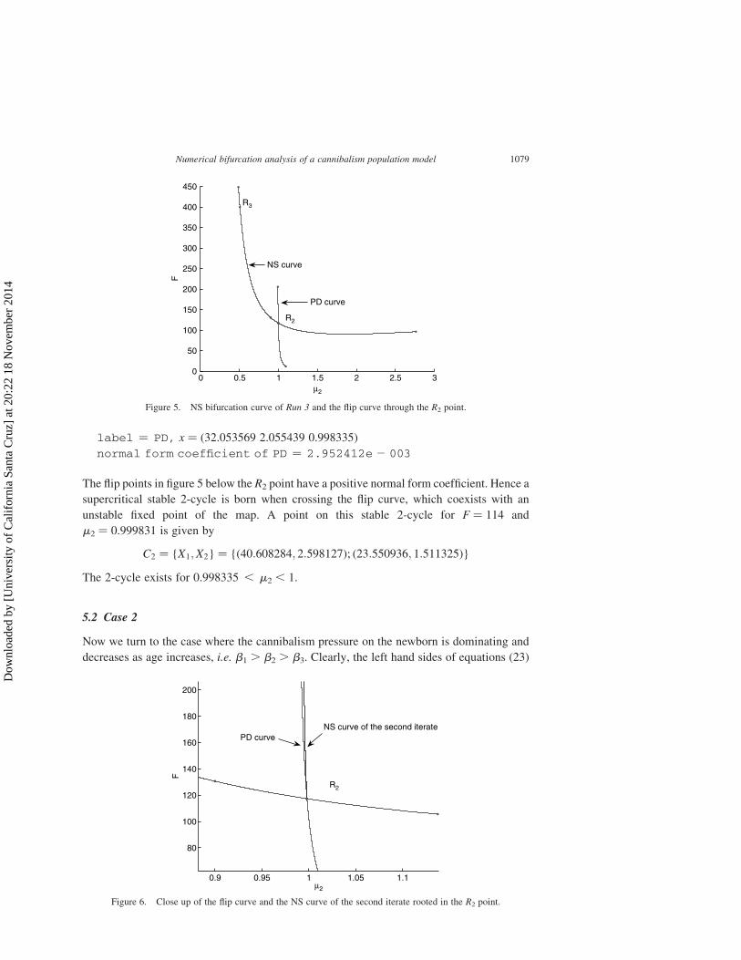
label ¼ PD, x ¼ (32.053569 2.055439 0.998335)


The flip points in figure 5 below the R2 point have a positive normal form coefficient. Hence a

supercritical stable 2-cycle is born when crossing the flip curve, which coexists with an

unstable fixed point of the map. A point on this stable 2-cycle for F ¼ 114 and

m2 ¼ 0.999831 is given by

C2 ¼ {X1;X2} ¼ {ð40:608284; 2:598127Þ; ð23:550936; 1:511325Þ}

The 2-cycle exists for 0.998335 , m2 , 1.

5.2 Case 2

Now we turn to the case where the cannibalism pressure on the newborn is dominating and

decreases as age increases, i.e. b1 . b2 . b3. Clearly, the left hand sides of equations (23)

Figure 5. NS bifurcation curve of Run 3 and the flip curve through the R2 point.

Figure 6. Close up of the flip curve and the NS curve of the second iterate rooted in the R2 point.


Dow

nloa

ded

by [

Uni

vers

ity o

f C

alif

orni

a Sa

nta

Cru

z] a

t 20:

22 1

8 N

ovem

ber

2014

and (24) are positive for small values of x*2, i.e. in this part of parameter space the fixed point

ðx*1; x

*2Þ is stable. A qualitative reasoning in Ref. [17] leads to the conclusion that both a NS

and a PD bifurcation are possible, but the latter only in a small parameter region.

For the numerical stability analysis of the fixed point, we consider the parameter set

m1 ¼ m2 ¼ P ¼ 0.5, F ¼ 55 and bi ¼ 4 2 i, i ¼ 1, 2, 3. For these parameters, the fixed point

ðx*1; x

*2Þ ¼ ð2:8213; 1:01868Þ is numerically computed from equations (18) and (19). We note

that it is an unstable fixed point. Now, in Run 5, we continue fixed points where F is the free

parameter.

label ¼ NS, x ¼ (2.718282 1.00000 50.903622)


label ¼ BP, x ¼ (20.00000 20.00000 0.50000)

Run 5 shows that the fixed point is stable for small values of the fecundity, i.e. between BP

and NS. When F exceeds the threshold Fc ¼ 50.903622, i.e. when the inequality sign in

equation (24) is reversed, we find a stable invariant curve. Now we continue with free

parameter b1. We refer to this as Run 6:

label ¼ NS, x ¼ (3.132638 1.072181 2.793847)


label ¼ PD, x ¼ (60.897776 3.007941 0.332657)

normal form coefficient of PD ¼ 3.603081e þ 001

The fixed point is stable between the PD and NS points, i.e. where b1 [ [2, 2.7987], b2 ¼ 2,

b3 ¼ 1. We proceed with the numerical investigation of stability where b2 is free, in Run 7:

label ¼ NS, x ¼ (2.932052 1.038207 1.258253)


We find that the fixed point is unstable before NS and stable afterwards, i.e. where b1 ¼ 3,

b2 [ [1, 1.258201], b3 ¼ 1. Next, we continue with b3 free, in Run 8:

label ¼ NS, x ¼ (2.926588 1.001660 1.070402)


label ¼ PD, x ¼ (8.864167 0.362921 8.805179)

normal form coefficient of PD ¼ 1.144210e þ 000

By monitoring the multipliers in Run 8, it is found that the fixed point is stable between the

NS and PD points, i.e. the fixed point is stable where b1 ¼ 3, b2 ¼ 2, b3 [ [1.070402, 2].

Since the normal form coefficient of the PD point is positive, a stable 2-cycle is born where

b3 . 8.805179. Moreover, it can be seen that increasing b3, the cannibalism of the immature

on the threshold of entering the mature age, results in a wider range of stability than

increasing b1.

For a further analysis, we ignore the condition b1 . b2 . b3 and compute the NS curve,

by starting at the NS point in Run 6, with free parameters F and b3, this is Run 9:


Dow

nloa

ded

by [

Uni

vers

ity o

f C

alif

orni

a Sa

nta

Cru

z] a

t 20:

22 1

8 N

ovem

ber

2014

label ¼ R4, x ¼ (3.119219 1.003084 58.799673 1.131015 0)

normal form coefficient of R4: A ¼ 24.610753e þ 00 þ 2 1.142472e þ 00 i

Since jAj.1 in the R4 point in Run 9, two cycles of period 4 of the map are born. The fixed

points Fk, k ¼ 1, 2, 3, 4 of the fourth iterate of the map which are closer to the original fixed

point are saddles, while the remote ones Sk, k ¼ 1, 2, 3, 4 are attractors. An exact stable

4-cycle for b3 ¼ 1.131015 and F ¼ 58.9 is given by C4 ¼ {X1, X2, X3, X4} where

X1 ¼ ð3:21494; 1:035797Þ; X2 ¼ ð2:93066; 1:01606Þ;

X3 ¼ ð3:031476; 0:97239Þ; X4 ¼ ð3:31453; 0:99085Þ:

We present this cycle in figure 7. The multipliers of the fourth iterate of the map in X1 are

l1 ¼ 0.999819 and l2 ¼ 0.996348, confirming the stability of the 4-cycle.

To compute the stability domain of the 4-cycle, we note that since jAj . 1, there are two

half-lines of fold bifurcation curves of the fourth iterate that emanate from the R4 point. We

present these lines in figure 8.

Figure 7. An exact 4-cycle for m1 ¼ m2 ¼ P ¼ 0.5, b1 ¼ 3, b2 ¼ 2, b3 ¼ 1.131015, F ¼ 58.9.

Figure 8. Two half-lines of fold bifurcation points emanate from an R4 point.


Dow

nloa

ded

by [

Uni

vers

ity o

f C

alif

orni

a Sa

nta

Cru

z] a

t 20:

22 1

8 N

ovem

ber

2014

For each set of parameter values in the wedge between the two half-lines both a stable 4-

cycle and an unstable 4-cycle exist. For fixed values of F larger than that of the R4 point the

fixed points of the fourth iterate form a closed curve that changes stability in two fold curves.

We note that the stable 4-cycles exist in a wide parameter region but there is no bistability

with fixed points of the original map.

The NS curve, starting from the NS point in Run 8, where m2 and b3 are free parameters, is

computed in Run 10:

label ¼ R4, x ¼ (3.011107 0.988367 0.511112 1.104883 20.000000)

NormalformcoefficientofR4:A ¼ 24.675831e þ 000 þ 2 1.079711e þ 000 i

label ¼ R3, x ¼ (5.026676 0.735955 0.910954 1.795572 20.500000)

Normal form coefficient of R3: Re(c_1) ¼ 21.581503e þ 000

label ¼ R2, x ¼ (6.1262370.627511 1.395201 1.995804 2 1.000000)

Normal form coefficient of R2:[c, d ] ¼ 6.737115e 2 002, 21.789198e 2 001

5.3 Case 3

In the last case, we assume b1 , b2 , b3. It is clear that the left hand sides of equations (23)

and (24) are positive where x*2 is small enough, i.e. there exists a parameter interval where

ðx*1; x

*2Þ is stable. When b1 < b2 < b3 (but b1 , b2 , b3), then the left hand side of

equation (24) is approximately equal to 1 þ ð1 2 b1x*2Þm2 2 ð12 m1Þe

2b2x*2 and can be

negative for some parameter values. This means that there exists a parameter region where a

NS bifurcation may occur. We note that in Case 3, the most dominating negative term

appears in equation (23). So, when b3 becomes large compared to b1, then ðb1 2 b3Þm2x*2 in

B becomes the dominating negative term, which strongly suggests that in this case there will

be a flip bifurcation at the instability threshold. We remark that in the next runs, we are

interested only in the range b1 , b2 , b3.

We consider the parameter set m1 ¼ m2 ¼ P ¼ 0:5, F ¼ 200 and bi ¼ i; i ¼ 1; 2; 3. The

fixed point

ðx*1; x

*2Þ ¼ ð72:8206; 1:33341Þ ð33Þ

is computed from equations (18) and (19). We note that this is an unstable fixed point. Now

we continue the fixed point (1) where F is the free parameter, we call this Run 11:

label ¼ PD, x ¼ (25.184229 1.056945 64.424674)


In Run 11, there is a supercritical flip bifurcation at the instability threshold, hence a stable 2-

cycle is born for F . 64.424674. The fixed point is unstable before the PD point and stable

afterwards. The new branch of fixed points of the second iterate is given in figure 9.

We proceed with the continuation of fixed points where b1 is free, we call this Run 12:

label ¼ PD, x ¼ (49.555931 1.231597 1.337322)


label ¼ NS, x ¼ (6.567122 0.731554 4.410725)



Dow

nloa

ded

by [

Uni

vers

ity o

f C

alif

orni

a Sa

nta

Cru

z] a

t 20:

22 1

8 N

ovem

ber

2014

The fixed point is stable between the PD and NS points, i.e. when b1 [ [1.337322, 2],

b2 ¼ 2, b3 ¼ 3. Due to the positive sign of the normal form coefficient of the PD point, a

stable 2-cycle coexists with the unstable fixed point of the map for b1 , 1.337322.

The fixed point ðx*1; x

*2Þ in equation (33), remains unstable under variation of the parameter

b2, hence increasing the cannibalism pressure on the immature part is not a stabilizing factor

from a dynamical point of view. We now continue with the free parameter b3, we call this

Run 13:

label ¼ PD, x ¼ (64.840130 1.640192 2.241879)


label ¼ NS, x ¼ (29.976635 2.996639 0.768503)


The fixed point is stable between the PD and NS points, i.e. when b1 ¼ 1;

b2 ¼ 2;b3 [ ½2; 2:241879�. From the sign of the normal form coefficient of the PD

point, we see that a stable 2-cycle is born when b3 exceeds the threshold stability

b3 ¼ 2.241879. An exact stable 2-cycle for P ¼ m1 ¼ m2 ¼ 0:5;b1 ¼ 1;b2 ¼ 2;b3 ¼

2:2510715 and F ¼ 200 is given by

C2 ¼ {X1;X2} ¼ {ð66:459403; 1:69537Þ; ð63:349999; 1:578968Þ}

We proceed with computing the NS curve encountered in Run 13, where F and b3 are free in

the continuation, we call this Run 14:

label ¼ R3, x ¼ (60.356868 2.997515 402.928800 1.001660 20.500000)


label ¼ R4, x ¼ (8.161668 2.995002 54.393960 0.334726 0.000000)


The R3 point has the same characteristics (i.e. normal form coefficients with the same sign) as

that in Run 3. The R4 point has the same characteristics (absolute value and sign of real and

imaginary part) as that in Run 9. By Run 14, there are unstable 3-cycles and stable 4-cycles of

Figure 9. Branch of fixed points of the second iterate and of the original map in (F, x1) space.


Dow

nloa

ded

by [

Uni

vers

ity o

f C

alif

orni

a Sa

nta

Cru

z] a

t 20:

22 1

8 N

ovem

ber

2014

fixed points near the R3 and R4 points, respectively. We continue by computing the NS curve

forth and back where m2 and b3 are the free parameters; we call this Run 15:

label ¼ R3, x ¼ (36.106260 2.711598 0.582753 0.898279 20.500000)


label ¼ R2, x ¼ (49.265517 2.192296 0.835266 1.185576 2 1.000000)

Normal form coefficient of R2: [c, d ] ¼ 25.112120e 2 004,21.100939e 2 003

label ¼ R4, x ¼ (16.751436 3.820439 0.354409 0.476980 20.000000)


The R3 and R2 points have the same characteristics (i.e. normal form coefficients with the

same sign) as those in Run 3. The R4 point has the same characteristics (absolute value and

sign of real and imaginary part) as that in Run 9.

6. Some conclusions and remarks

In Case 1 (b1 ¼ b2 ¼ b3), we mainly focused on the interplay between increased fecundity

and death rate while in Case 2 (b1 . b2 . b3) and Case 3 (b1 , b2 , b3), we focused on

the interplay between increased fecundity and increased cannibalism pressure. The

numerical computations in the previous sections show that in all cases there exists a large

parameter region where the nontrivial fixed point is stable. In Case 1, the transfer from

stability to instability usually goes through a NS bifurcation under variation of the fecundity

F. The NS bifurcation point is supercritical. Beyond the NS point the dynamics is restricted

to a stable invariant curve that surrounds the unstable fixed point. For large values of F (and

variable m2), periodic orbits of period 3.2k, k ¼ 0, 1, 2, . . . , a cascade of period doublings,

appears. However, these periodic orbits are unstable. For small values of F (and variable m2),

the nontrivial fixed point ðx*1; x

*2Þ coexists with a stable 2-cycle.

In Case 2, the transfer from stability to instability usually goes through a NS bifurcation

under variation of the fecundity F. The NS bifurcation point is supercritical.

In Case 3, stability is usually lost through a PD bifurcation.

In Cases 2 and 3, there are stable 4-cycles. An important point is that the effect of

increasing the cannibalism pressures b1, b2 and b3 is not the same. In Case 2, the fixed

point is stable for b3 [ [1.070402, 2] which is the widest stability range. In Case 3, we

see that the fixed point remains stable for b1 [ [1.337322, 2] which is the largest region

of stability.

The detected and computed strong resonance points (R2, R3, R4) serve as organizing

centres for the found stable and unstable 2-, 3- and 4-cycles. In the R2 case, we computed a

NS curve of the second iterate that emanates from the R2 point and forms a stability boundary

for 2-cycles. In the R3 case, we found a nearby stability region for 3-cycles that is bounded

by fold and flip curves. In the R4 case, we computed stability boundaries for 4-cycles as fold

curves of 4-cycles.

With these results many observations made in Ref. [17] can now be understood in a precise

way and the transition points can be computed accurately. E.g., the discussion at the end of

Ref. [17, Section 3, Case 2] (description of the birth of a stable 4-cycle) is now clarified by

the knowledge that in fact we have a fold bifurcation of 4-cycles which can be computed

accurately.


Dow

nloa

ded

by [

Uni

vers

ity o

f C

alif

orni

a Sa

nta

Cru

z] a

t 20:

22 1

8 N

ovem

ber

2014

Acknowledgements

It is a pleasure to thank our colleague at Ghent University Andre Vanderbauwhede for the

years of collaboration and joint organization of various activities related to our research in

dynamical systems. We also thank Yuri A. Kuznetsov and Hil Meijer from Utrecht University

for the intensive collaboration and their advice on this and other work. We also thank an

anonymous referee for several useful suggestions that have considerably improved the paper.

References

[1] Allgower, E.L. and Georg, K., 1990, Numerical Continuation Methods: An Introduction (New York: Springer-Verlag).

[2] Caswell, H., 2001, Matrix Population Models (Sunderland, MA: Sinaur Ass. Inc. Publishers).[3] Cushing, J.M., Costantino, R.F., Dennis, B., Deshamias, R.A. and Henson, A.M., 1998, Nonlinear population

dynamics: models, experiments and data. Journal of Theoretical Biology, 194, 1–9.[4] Dennis, B., Deshamais, R.A., Cushing, J.M. and Costantino, R.F., 1997, Transition in population dynamics:

equilibria to periodic cycles to aperiodic cycles. Journal of Animal Ecology, 6b, 704–729.[5] Dhooge, A., Govaerts, W. and Kuznetsov, Y.A., 2003, MatCont: a Matlab package for numerical bifurcation

analysis of ODEs. ACM Transactions on Mathematical Software, 29(2), 141–164.[6] Dhooge, A., Govaerts, W., Kuznetsov, Y.A., Mestrom, W. and Riet, A., 2004, Cl_MATCONT: a continuation

toolbox in Matlab, http://www.matcont.UGent.be.[7] Fox, J.D., 1975, Cannibalism in natural populations. Annual Review of Ecology and Systematics, 6, 87–106.[8] Govaerts, W. and Khoshsiar Ghaziani, R., Matlab software for bifurcations of maps and its application to a

Leslie–Gower model, Proceedings of the Fifth EUROMECH Nonlinear Dynamics Conference, Eindhoven,The Netherlands, August 7–12, ENOC-2005., 1740–1749.

[9] Govaerts, W., Khoshsiar Ghaziani, R., Kuznetsov, Y.A. and Meijer, H., 2006, Bifurcation analysis of periodicorbits of maps in Matlab, preprint.

[10] Kuznetsov, Y.A., 2004, Elements of Applied Bifurcation Theory, 3rd ed. (New York: Springer-Verlag).[11] Kuznetsov, Y.A. and Meijer, H.G.E., 2005, Numerical normal forms for codim 2 bifurcations of maps with at

most two critical eigenvalues. SISC, 26(6), 1932–1954.[12] Linehan, J.E., Gregpy, R.S. and Schneider, D.C., 2001, Predation risk of age-0 cod(Gadus) relative to depth

and substrate in coastal water. Journal of Experimental Marine Biology and Ecology, 263, 25–44.[13] Murray, J.D., 1993, Mathematical Biology, 2nd ed. (Berlin, Heidelberg, NY: Springer).[14] Myers, R.A., Blanchard, W. and Thompson, K.R., 1990, Summary of North Atlantic fish recruitment 1942–

1987. Canadian Technical Report of Fisheries and Aquatic Sciencies, 1743.[15] Ottersen, G., 1996, Environmental impact on variability in recruitment, larval growth and distribution of

Arcto–Norwegian cod, Dr Scient thesis, Geophysical Institute, University of Bergen.[16] Polis, G.A., 1981, The evolution and dynamics of intraspecific predation. Annual Review of Ecology and

Systematics, 12, 225–251.[17] Wikan, A. and Eide, A., 2004, An analysis of a nonlinear stage-structured cannibalism model with application

to the Northeast Arctic cod stock. Bulletin of Mathematical Biology, 66, 1685–1704.[18] Wikan, A. and Mjølhus, E., 1996, Overcompensatory recruitment and generation delay in discrete age-

structured population models. Journal of Mathematical Biology, 35, 195–239.


Dow

nloa

ded

by [

Uni

vers

ity o

f C

alif

orni

a Sa

nta

Cru

z] a

t 20:

22 1

8 N

ovem

ber

2014

numerical bifurcation analysis of a nonlinear stage structured cannibalism population model

Documents