numerical differentiation and...

師大

Numerical Differentiation and Integration

Tsung-Ming Huang

Department of MathematicsNational Taiwan Normal University, Taiwan

January 1, 2008

T.M. Huang (Nat. Taiwan Normal Univ.) Numerical Diff. & integ. January 1, 2008 1 / 31

師大

Outline

1 Numerical Differentiation

2 Richardson Extrapolation Method

3 Elements of Numerical IntegrationNewton-Cotes FormulasComposite Newton-Cotes Forumlas


師大

Numerical Differentiation

f ′(x0) = limh→0

f(x0 + h)− f(x0)h

.

Question

How accurate is

f(x0 + h)− f(x0)h

?

Suppose a given function f has continuous first derivative and f ′′ exists.From Taylor’s theorem

f(x + h) = f(x) + f ′(x)h +12f ′′(ξ)h2,

where ξ is between x and x + h, one has

f ′(x) =f(x + h)− f(x)

h− h

2f ′′(ξ) =

f(x + h)− f(x)h

+ O(h).


師大

Hence it is reasonable to use the approximation

f ′(x) ≈ f(x + h)− f(x)h

which is called forward finite difference, and the error involved is

|e| = h

2|f ′′(ξ)| ≤ h

2max

t∈(x,x+h)|f ′′(t)|.

Similarly one can derive the backward finite difference approximation

f ′(x) ≈ f(x)− f(x− h)h

(1)

which has the same order of truncation error as the forward finitedifference scheme.


師大

The forward difference is an O(h) scheme. An O(h2) scheme can also bederived from the Taylor’s theorem

f(x + h) = f(x) + f ′(x)h +12f ′′(x)h2 +

16f ′′′(ξ1)h3

f(x− h) = f(x)− f ′(x)h +12f ′′(x)h2 − 1

6f ′′′(ξ2)h3,

where ξ1 is between x and x + h and ξ2 is between x and x− h. Hence

f(x + h)− f(x− h) = 2f ′(x)h +16[f ′′′(ξ1) + f ′′′(ξ2)]h3

and

f ′(x) =f(x + h)− f(x− h)

2h− 1

12[f ′′′(ξ1) + f ′′′(ξ2)]h2

LetM = max

z∈[x−h,x+h]f ′′′(z) and m = min

z∈[x−h,x+h]f ′′′(z).


師大

If f ′′′ is continuous on [x− h, x + h], then by the intermediate valuetheorem, there exists ξ ∈ [x− h, x + h] such that

f ′′′(ξ) =12[f ′′′(ξ1) + f ′′′(ξ2)].

Hence

f ′(x) =f(x + h)− f(x− h)

2h− 1

6f ′′′(ξ)h2 =

f(x + h)− f(x− h)2h

+ O(h2).

This is called center difference approximation and the truncation error is

|e| = h2

6f ′′′(ξ)

Similarly, we can derive an O(h2) scheme from Taylor’s theorem for f ′′(x)

f ′′(x) =f(x + h)− 2f(x) + f(x− h)

h2− 1

12f (4)(ξ)h2,

where ξ is between x− h and x + h.


師大

Polynomial Interpolation MethodSuppose that (x0, f(x0)), (x1, f(x1)) · · · , (xn, f(xn) have been given, weapply the Lagrange polynomial interpolation scheme to derive

P (x) =n∑

i=0

f(xi)Li(x),

where

Li(x) =n∏

j=0,j 6=i

x− xj

xi − xj.

Since f(x) can be written as

f(x) =n∑

i=0

f(xi)L(x) +1

(n + 1)!f (n+1)(ξx)w(x),

where

w(x) =n∏

j=0

(x− xj),


師大

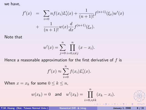
we have,

f ′(x) =∑i=0

nf(xi)L′i(x) +1

(n + 1)!f (n+1)(ξx)w′(x)

+1

(n + 1)!w(x)

d

dxf (n+1)(ξx).

Note that

w′(x) =n∑

j=0

n∏i=0,i6=j

(x− xi).

Hence a reasonable approximation for the first derivative of f is

f ′(x) ≈n∑

i=0

f(xi)L′i(x).

When x = xk for some 0 ≤ k ≤ n,

w(xk) = 0 and w′(xk) =n∏

i=0,i6=k

(xk − xi).


師大

Hence

f ′(xk) =n∑

i=0

f(xi)L′i(xk) +1

(n + 1)!f (n+1)(ξx)

n∏i=0,i6=k

(xk − xi), (2)

which is called an (n + 1)-point formula to approximate f ′(x).• Three Point FormulasSince

L0(x) =(x− x1)(x− x2)

(x0 − x1)(x0 − x2)

we have

L′0(x) =2x− x1 − x2

(x0 − x1)(x0 − x2).

Similarly,

L′1(x) =2x− x0 − x2

(x1 − x0)(x1 − x2)and L′2(x) =

2x− x0 − x1

(x2 − x0)(x2 − x1).


師大

Hence

f ′(xj) = f(x0)[

2xj − x1 − x2

(x0 − x1)(x0 − x2)

]+ f(x1)

[2xj − x0 − x2

(x1 − x0)(x1 − x2)

]+ f(x2)

[2xj − x0 − x1

(x2 − x0)(x2 − x1)

]+

16f (3)(ξj)

2∏k=0,k 6=j

(xj − xk),

for each j = 0, 1, 2. Assume that

x1 = x0 + h and x2 = x0 + 2h, for some h 6= 0.

Then

f ′(x0) =1h

[−3

2f(x0) + 2f(x1)−

12f(x2)

]+

h2

3f (3)(ξ0),

f ′(x1) =1h

[−1

2f(x0) +

12f(x2)

]− h2

6f (3)(ξ1),

f ′(x2) =1h

[12f(x0)− 2f(x1) +

32f(x2)

]+

h2

3f (3)(ξ2).


師大

That is

f ′(x0) =1h

[−3

2f(x0) + 2f(x0 + h)− 1

2f(x0 + 2h)

]+

h2

3f (3)(ξ0),

f ′(x0 + h) =1h

[−1

2f(x0) +

12f(x0 + 2h)

]− h2

6f (3)(ξ1), (3)

f ′(x0 + 2h) =1h

[12f(x0)− 2f(x0 + h) +

32f(x0 + 2h)

]+

h2

3f (3)(ξ2).(4)

Using the variable substitution x0 for x0 + h and x0 + 2h in (3) and (4),respectively, we have

f ′(x0) =12h

[−3f(x0) + 4f(x0 + h)− f(x0 + 2h)] +h2

3f (3)(ξ0),(5)

f ′(x0) =12h

[−f(x0 − h) + f(x0 + h)]− h2

6f (3)(ξ1),

f ′(x0) =12h

[f(x0 − 2h)− 4f(x0 − h) + 3f(x0)] +h2

3f (3)(ξ2). (6)

Note that (6) can be obtained from (5) by replacing h with −h.T.M. Huang (Nat. Taiwan Normal Univ.) Numerical Diff. & integ. January 1, 2008 11 / 31

師大

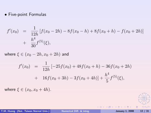
• Five-point Formulas

f ′(x0) =1

12h[f(x0 − 2h)− 8f(x0 − h) + 8f(x0 + h)− f(x0 + 2h)]

+h4

30f (5)(ξ),

where ξ ∈ (x0 − 2h, x0 + 2h) and

f ′(x0) =1

12h[−25f(x0) + 48f(x0 + h)− 36f(x0 + 2h)

+ 16f(x0 + 3h)− 3f(x0 + 4h)] +h4

5f (5)(ξ),

where ξ ∈ (x0, x0 + 4h).


師大

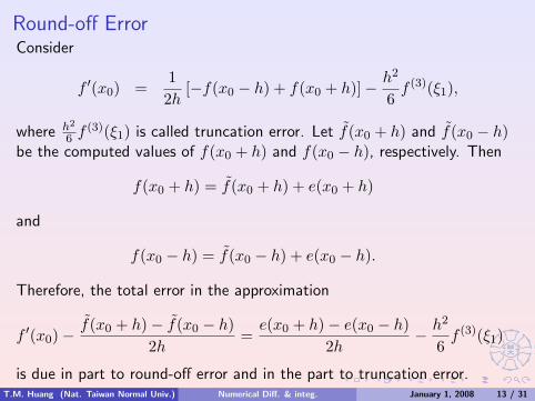
Round-off ErrorConsider

f ′(x0) =12h

[−f(x0 − h) + f(x0 + h)]− h2

6f (3)(ξ1),

where h2

6 f (3)(ξ1) is called truncation error. Let f̃(x0 + h) and f̃(x0 − h)be the computed values of f(x0 + h) and f(x0 − h), respectively. Then

f(x0 + h) = f̃(x0 + h) + e(x0 + h)

and

f(x0 − h) = f̃(x0 − h) + e(x0 − h).

Therefore, the total error in the approximation

f ′(x0)−f̃(x0 + h)− f̃(x0 − h)

2h=

e(x0 + h)− e(x0 − h)2h

− h2

6f (3)(ξ1)

is due in part to round-off error and in the part to truncation error.T.M. Huang (Nat. Taiwan Normal Univ.) Numerical Diff. & integ. January 1, 2008 13 / 31

師大

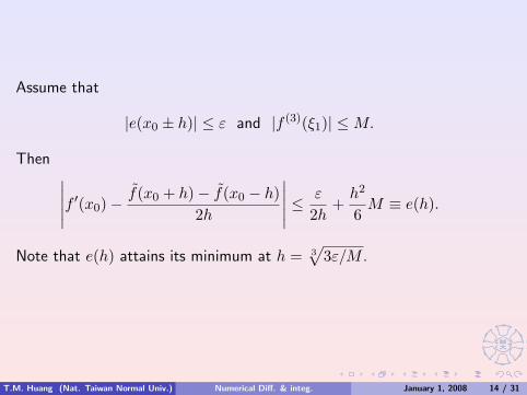
Assume that

|e(x0 ± h)| ≤ ε and |f (3)(ξ1)| ≤ M.

Then ∣∣∣∣∣f ′(x0)−f̃(x0 + h)− f̃(x0 − h)

2h

∣∣∣∣∣ ≤ ε

2h+

h2

6M ≡ e(h).

Note that e(h) attains its minimum at h = 3√

3ε/M .


師大

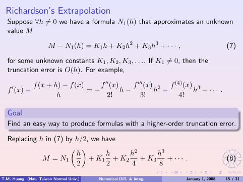
Richardson’s ExtrapolationSuppose ∀h 6= 0 we have a formula N1(h) that approximates an unknownvalue M

M −N1(h) = K1h + K2h2 + K3h

3 + · · · , (7)

for some unknown constants K1,K2,K3, . . .. If K1 6= 0, then thetruncation error is O(h). For example,

f ′(x)− f(x + h)− f(x)h

= −f ′′(x)2!

h− f ′′′(x)3!

h2 − f (4)(x)4!

h3 − · · · .

Goal

Find an easy way to produce formulas with a higher-order truncation error.

Replacing h in (7) by h/2, we have

M = N1

(h

2

)+ K1

h

2+ K2

h2

4+ K3

h3

8+ · · · . (8)


師大

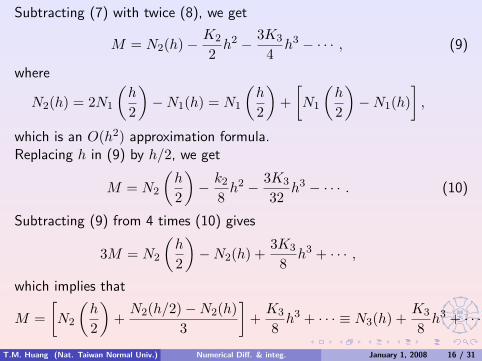
Subtracting (7) with twice (8), we get

M = N2(h)− K2

2h2 − 3K3

4h3 − · · · , (9)

where

N2(h) = 2N1

(h

2

)−N1(h) = N1

(h

2

)+

[N1

(h

2

)−N1(h)

],

which is an O(h2) approximation formula.Replacing h in (9) by h/2, we get

M = N2

(h

2

)− k2

8h2 − 3K3

32h3 − · · · . (10)

Subtracting (9) from 4 times (10) gives

3M = N2

(h

2

)−N2(h) +

3K3

8h3 + · · · ,

which implies that

M =[N2

(h

2

)+

N2(h/2)−N2(h)3

]+

K3

8h3 + · · · ≡ N3(h) +

K3

8h3 + · · · .


師大

Using induction, M can be approximated by

M = Nm(h) + O(hm),

where

Nm(h) = Nm−1

(h

2

)+

Nm−1(h/2)−Nm−1(h)2m−1 − 1

.

Centered difference formula. From the Taylor’s theorem

f(x + h) = f(x) + hf ′(x) +h2

2!f ′′(x) +

h3

3!f ′′′(x) +

h4

4!f (4)(x) +

h5

5!f (5)(x) +

h6

6!f (6)(x) + · · ·

f(x− h) = f(x)− hf ′(x) +h2

2!f ′′(x)− h3

3!f ′′′(x) +

h4

4!f (4)(x)− h5

5!f (5)(x) +

h6

6!f (6)(x) + · · ·

we have

f(x + h)− f(x− h) = 2hf ′(x) +2h3

3!f ′′′(x) +

2h5

5!f (5)(x) + · · · ,


師大

and, consequently,

f ′(x0) =f(x0 + h)− f(x0 − h)

2h−

[h2

3!f ′′′(x0) +

h4

5!f (5)(x0) + · · ·

],

≡ N1(h)−[h2

3!f ′′′(x0) +

h4

5!f (5)(x0) + · · ·

]. (11)

Replacing h in (11) by h/2 gives

f ′(x0) = N1

(h

2

)− h2

24f ′′′(x0)−

h4

1920f (5)(x0)− · · · . (12)

Subtracting (11) from 4 times (12) gives

f ′(x0) = N2(h) +h4

480f (5)(x0) + · · · ,

where

N2(h) =13

[4N1

(h

2

)−N1(h)

]= N1

(h

2

)+

N1(h/2)−N1(h)3

.


師大

In general,

f ′(x0) = Nj(h) + O(h2j)

with

Nj(h) = Nj−1

(h

2

)+

Nj−1(h/2)−Nj−1(h)4j−1 − 1

.

Example

Suppose that x0 = 2.0, h = 0.2 and f(x) = xex. Compute anapproximated value of f ′(2.0) = 22.16716829679195 to six decimal places.

Solution. By centered difference formula, we have

N1(0.2) =f(0.2 + h)− f(0.2− h)

2h= 22.414160,

N1(0.1) =f(0.1 + h)− f(0.1− h)

2h= 22.228786.


師大

It implies that

N2(0.2) = N1(0.1) +N1(0.1)−N1(0.2)

3= 22.166995

which does not have six decimal digits. Adding N1(0.05) = 22.182564, weget

N2(0.1) = N1(0.05) +N1(0.05)−N1(0.1)

3= 22.167157

and

N3(0.2) = N2(0.1) +N2(0.1)−N2(0.2)

15= 22.167168

which contains six decimal digits.


師大

O(h) O(h2) O(h3) O(h4)1: N1(h) = N(h)2: N1(h/2) = N(h/2) 3: N2(h)4: N1(h/4) = N(h/4) 5: N2(h/2) 6: N3(h)7: N1(h/8) = N(h/8) 8: N2(h/4) 9: N3(h/2) 10: N4(h)


師大

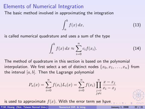
Elements of Numerical IntegrationThe basic method involved in approximating the integration∫ b

af(x) dx, (13)

is called numerical quadrature and uses a sum of the type∫ b

af(x) dx ≈

n∑i=0

cif(xi). (14)

The method of quadrature in this section is based on the polynomialinterpolation. We first select a set of distinct nodes {x0, x1, . . . , xn} fromthe interval [a, b]. Then the Lagrange polynomial

Pn(x) =n∑

i=0

f(xi)Li(x) =n∑

i=0

f(xi)n∏

j=0

j 6=i

x− xj

xi − xj

is used to approximate f(x). With the error term we haveT.M. Huang (Nat. Taiwan Normal Univ.) Numerical Diff. & integ. January 1, 2008 22 / 31

師大

f(x) = Pn(x) + En(x) =n∑

i=0

f(xi)Li(x) +f (n+1)(ζx)(n + 1)!

n∏i=0

(x− xi),

where ζx ∈ [a, b] and depends on x, and∫ b

af(x) dx =

∫ b

aPn(x) dx +

∫ b

aEn(x) dx

=n∑

i=0

f(xi)∫ b

aLi(x) dx +

1(n + 1)!

∫ b

af (n+1)(ζx)

n∏i=0

(x− xi) dx.(15)

The quadrature formula is, therefore,∫ b

af(x) dx ≈

∫ b

aPn(x) dx =

n∑i=0

f(xi)∫ b

aLi(x) dx ≡

n∑i=0

cif(xi), (16)

where

ci =∫ b

aLi(x) dx =

∫ b

a

n∏j=0

j 6=i

x− xj

xi − xjdx. (17)


師大

Moreover, the error in the quadrature formula is given by

E =1

(n + 1)!

∫ b

af (n+1)(ζx)

n∏i=0

(x− xi) dx, (18)

for some ζx ∈ [a, b].Let us consider formulas produced by using first and second Lagrangepolynomials with equally spaced nodes. This gives the Trapezoidal ruleand Simpson’s rule, respectively.Trapezoidal rule: Let x0 = a, x1 = b, h = b− a and use the linearLagrange polynomial:

P1(x) =(x− x1)(x0 − x1)

f(x0) +(x− x0)(x1 − x0)

f(x1).

Then ∫ b

af(x)dx =

∫ x1

x0

[(x− x1)(x0 − x1)

f(x0) +(x− x0)(x1 − x0)

f(x1)]

dx

+12

∫ x1

x0

f ′′(ζ(x))(x− x0)(x− x1)dx. (19)


師大

Theorem (Weighted Mean Value Theorem for Integrals)

Suppose f ∈ C[a, b], the Riemann integral of g(x)∫ b

ag(x)dx = lim

max4xi→0

n∑i=1

g(xi)4xi,

exists and g(x) does not change sign on [a, b]. Then ∃ c ∈ (a, b) with∫ b

af(x)g(x)dx = f(c)

∫ b

ag(x)dx.

Since (x− x0)(x− x1) does not change sign on [x0, x1], by the WeightedMean Value Theorem, ∃ ζ ∈ (x0, x1) such that∫ x1

x0

f ′′(ζ(x))(x− x0)(x− x1)dx = f ′′(ζ)∫ x1

x0

(x− x0)(x− x1)dx

= f ′′(ζ)[x3

3− x1 + x0

2x2 + x0x1x

]x1

x0

= −h3

6f ′′(ζ).


師大

Consequently, Eq. (19) implies that∫ b

af(x)dx =

[(x− x1)2

2(x0 − x1)f(x0) +

(x− x0)2

2(x1 − x0)f(x1)

]x1

x0

− h3

12f ′′(ζ)

=x1 − x0

2[f(x0) + f(x1)]−

h3

12f ′′(ζ)

=h

2[f(x0) + f(x1)]−

h3

12f ′′(ζ),

which is called the Trapezoidal rule.


師大

If we choose x0 = a, x1 = 12(a + b), x2 = b, h = (b− a)/2, and the

second order Lagrange polynomial

P2(x) = f(x0)(x− x1)(x− x2)

(x0 − x1)(x0 − x2)+ f(x1)

(x− x0)(x− x2)(x1 − x0)(x1 − x2)

+f(x2)(x− x0)(x− x1)

(x2 − x0)(x2 − x1)

to interpolate f(x), then


師大

∫ b

af(x)dx =

∫ x2

x0

[(x− x1)(x− x2)

(x0 − x1)(x0 − x2)f(x0) +

(x− x0)(x− x2)(x1 − x0)(x1 − x2)

f(x1)

+(x− x0)(x− x1)

(x2 − x0)(x2 − x1)f(x2)

]dx

+∫ x2

x0

(x− x0)(x− x1)(x− x2)6

f (3)(ζ(x))dx.

Since, letting x = x0 + th,∫ x2

x0

(x− x1)(x− x2)(x0 − x1)(x0 − x2)

dx = h

∫ 2

0

t− 10− 1

· t− 20− 2

dt

=h

2

∫ 2

0(t2 − 3t + 2) dt =

h

3,∫ x2

x0

(x− x0)(x− x2)(x1 − x0)(x1 − x2)

dx = h

∫ 2

0

t− 01− 0

· t− 21− 2

dt

= −h

∫ 2

0(t2 − 2t) dt =

4h

3,


師大

∫ x2

x0

(x− x0)(x− x1)(x2 − x0)(x2 − x1)

dx = h

∫ 2

0

t− 02− 0

· t− 12− 1

dt

=h

2

∫ 2

0(t2 − t) dt =

h

3,

it implies that∫ b

af(x)dx = h

[13f(x0) +

43f(x1) +

13f(x2)

]+

∫ x2

x0

(x− x0)(x− x1)(x− x2)6

f (3)(ζ(x))dx,

which is called the Simpson’s rule.Deriving Simpson’s rule in this way, however, provides only an O(h4) errorterm involving f (3). A higher order error analysis can be derived byexpanding f in the third Taylor’s formula about x1. Then for eachx ∈ [a, b], there exists ζx ∈ (a, b) such that

f(x) = f(x1) + f ′(x1)(x− x1) +f ′′(x1)

2(x− x1)2

+f ′′′(x1)

6(x− x1)3 +

f (4)(ζx)24

(x− x1)4.T.M. Huang (Nat. Taiwan Normal Univ.) Numerical Diff. & integ. January 1, 2008 29 / 31

師大

Then∫ b

af(x) dx =

[f(x1)(x− x1) +

f ′(x1)2

(x− x1)2 +f ′′(x1)

6(x− x1)3

+f ′′′(x1)

24(x− x1)4

] ∣∣∣∣∣b

a

+124

∫ b

af (4)(ζx)(x− x1)4 dx.

Note that (b− x1) = h, (a− x1) = −h, and since (x− x1)4 does notchange sign in [a, b], by the Weighted Mean-Value Theorem for Integral,there exists ξ1 ∈ (a, b) such that∫ b

af (4)(ζx)(x− x1)4 dx = f (4)(ξ1)

∫ b

a(x− x1)4 dx =

2f (4)(ξ1)5

h5.

Consequently,∫ b

af(x) dx = 2f(x1)h +

f ′′(x1)3

h3 +f (4)(ξ1)

60h5.


師大

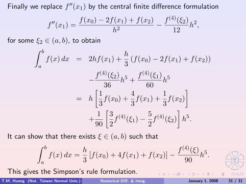
Finally we replace f ′′(x1) by the central finite difference formulation

f ′′(x1) =f(x0)− 2f(x1) + f(x2)

h2− f (4)(ξ2)

12h2,

for some ξ2 ∈ (a, b), to obtain∫ b

af(x) dx = 2hf(x1) +

h

3(f(x0)− 2f(x1) + f(x2))

−f (4)(ξ2)36

h5 +f (4)(ξ1)

60h5

= h

[13f(x0) +

43f(x1) +

13f(x2)

]+

190

[32f (4)(ξ1)−

52f (4)(ξ2)

]h5.

It can show that there exists ξ ∈ (a, b) such that∫ b

af(x) dx =

h

3[f(x0) + 4f(x1) + f(x2)]−

f (4)(ξ)90

h5.

This gives the Simpson’s rule formulation.T.M. Huang (Nat. Taiwan Normal Univ.) Numerical Diff. & integ. January 1, 2008 31 / 31

師大

If |f (n+1)(x)| ≤ M on [a, b], then∣∣∣∣∣∫ b

af(x) dx−

n∑i=0

cif(xi)

∣∣∣∣∣ ≤ M

(n + 1)!

∫ b

a

n∏i=0

(x− xi) dx. (20)

The choice of nodes that makes the right-hand side of this error bound assmall as possible is know to be

xi =a + b

2+

b− a

2cos

[(i + 1)πn + 2

], i = 0, 1, . . . , n. (21)

Of course, a polynomial interpolation to f can be obtained in other ways,for example, polynomial in Newton’s form using divided-difference method,

Pn(x) = f(x0) +n∑

i=1

f [x0, x1, . . . , xi]i−1∏j=0

(x− xj)

where f [x0, x1, . . . , xi] are evaluated with the divided difference algorithm.Then∫ b

af(x) dx ≈ f(x0)(b−a)+

n∑i=1

f [x0, x1, . . . , xi]∫ b

a

i−1∏j=0

(x−xj) dx. (22)


師大

The standard derivation of quadrature error formulas is based ondetermining the class of polynomials for which theses formulas produceexact results. The next definition is used to facilitate the discussion of thisderivation.

Definition

The degree of accuracy, or precision, of a quadrature formula is the largestpositive integer n such that the formula is exact for xk, whenk = 0, 1, . . . , n.

The definition implies that the degree of accuracy of a quadrature formulais n if and only if the error E = 0 for all polynomials P (x) of degree lessthan or equal to n, but E 6= 0 for some polynomials of degree greater thann.A quadrature formula of the form (14) is called a Newton-Cotes formula ifthe nodes {x0, x1, . . . , xn} are equally spaced. Consider a uniformpartition of the closed interval [a, b] by

xi = a + ih, i = 0, 1, . . . , n, h =b− a

n,


師大

where n is a positive integer and h is called the step length. Byintroduction a new variable t such that x = a + ht, the fundamentalLagrange polynomial becomes

Li(x) =n∏

j=0

j 6=i

x− xj

xi − xj=

n∏j=0

j 6=i

a + ht− a− jh

a + ih− a− jh=

n∏j=0

j 6=i

t− j

i− j≡ ϕi(t).

Therefore, the integration (17) gives

ci =∫ b

aLi(x) dx =

∫ n

0ϕi(t)h dt = h

∫ n

0

n∏j=0

j 6=i

t− j

i− jdt, (23)

and the general Newton-Cotes formula has the form∫ b

af(x) dx = h

n∑i=0

f(xi)∫ n

0

n∏j=0

j 6=i

t− j

i− jdt+

1(n + 1)!

∫ b

af (n+1)(ζx)

n∏i=0

(x−xi) dx.

(24)T.M. Huang (Nat. Taiwan Normal Univ.) Numerical Diff. & integ. January 1, 2008 31 / 31

師大

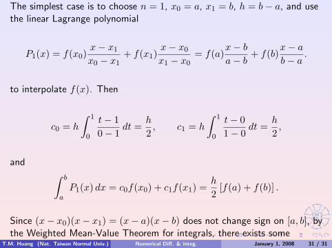
The simplest case is to choose n = 1, x0 = a, x1 = b, h = b− a, and usethe linear Lagrange polynomial

P1(x) = f(x0)x− x1

x0 − x1+ f(x1)

x− x0

x1 − x0= f(a)

x− b

a− b+ f(b)

x− a

b− a.

to interpolate f(x). Then

c0 = h

∫ 1

0

t− 10− 1

dt =h

2, c1 = h

∫ 1

0

t− 01− 0

dt =h

2,

and ∫ b

aP1(x) dx = c0f(x0) + c1f(x1) =

h

2[f(a) + f(b)] .

Since (x− x0)(x− x1) = (x− a)(x− b) does not change sign on [a, b], bythe Weighted Mean-Value Theorem for integrals, there exists some


師大

ξ ∈ (a, b) such that∫ b

af ′′(ζx)(x− x0)(x− x1) dx = f ′′(ξ)

∫ b

a(x− x0)(x− x1) dx

= f ′′(ξ)∫ b

a(x− a)(x− b) dx

= f ′′(ξ)[13x3 − 1

2(a + b)x2 + abx

] ∣∣∣∣∣b

a

= −16f ′′(ξ)(b− a)3 = −1

6f ′′(ξ)h3.

Consequently, ∫ b

af(x) dx =

h

2[f(a) + f(b)]− h3

12f ′′(ξ).

This gives the so-called Trapezoidal rule.Trapezoidal Rule:∫ b

af(x) dx =

12(b− a) [f(a) + f(b)]− h3

12f ′′(ξ), (25)


師大

where h = b− a and ξ ∈ (a, b).It is evident that the error term of the Trapezoidal rule is O(h3). Since therule involves f ′′, it gives the exact result when applied to any functionwhose second derivative is identically zero, e.g., any polynomial of degree1 or less. Hence the degree of accuracy of Trapezoidal rule is one.If we choose n = 2, x0 = a, x1 = 1

2(a + b), x2 = b, h = (b− a)/2, and thesecond order Lagrange polynomial

P2(x) = f(x0)(x− x1)(x− x2)

(x0 − x1)(x0 − x2)+f(x1)

(x− x0)(x− x2)(x1 − x0)(x1 − x2)

+f(x2)(x− x0)(x− x1)

(x2 − x0)(x2 − x1)

to interpolate f(x), then

c0 = h

∫ 2

0

t− 10− 1

· t− 20− 2

dt =h

2

∫ 2

0(t2 − 3t + 2) dt =

h

3,

c1 = h

∫ 2

0

t− 01− 0

· t− 21− 2

dt = −h

∫ 2

0(t2 − 2t) dt =

4h

3,

c2 = h

∫ 2

0

t− 02− 0

· t− 12− 1

dt =h

2

∫ 2

0(t2 − t) dt =

h

3,


師大

and

∫ b

aP2(x) dx = c0f(x0)+c1f(x1)+c2f(x2) = h

[13f(a) +

43f(

a + b

2) +

13f(b)

]

gives the so-called Simpson’s rule. Deriving the formulation this way,however, the error term

16

∫ b

af (3)(ζx)(x− x0)(x− x1)(x− x2) dx

provides only an O(h4) formulation involving f (3). A higher order erroranalysis can be derived by expanding f in the third Taylor’s formula aboutx1. Then for each x ∈ [a, b], there exists ζx ∈ (a, b) such that

f(x) = f(x1)+f ′(x1)(x−x1)+f ′′(x1)

2(x−x1)2+

f ′′′(x1)6

(x−x1)3+f (4)(ζx)

24(x−x1)4.


師大

Then∫ b

af(x) dx =

[f(x1)(x− x1) +

f ′(x1)2

(x− x1)2 +f ′′(x1)

6(x− x1)3 +

f ′′′(x1)24

(x− x1)4] ∣∣∣∣∣

b

a

+124

∫ b

af (4)(ζx)(x− x1)4 dx.

Note that (b− x1) = h, (a− x1) = −h, and since (x− x1)4 does notchange sign in [a, b], by the Weighted Mean-Value Theorem for Integral,there exists ξ1 ∈ (a, b) such that∫ b

af (4)(ζx)(x− x1)4 dx = f (4)(ξ1)

∫ b

a(x− x1)4 dx =

2f (4)(ξ1)5

h5.

Consequently,∫ b

af(x) dx = 2f(x1)h +

f ′′(x1)3

h3 +f (4)(ξ1)

60h5.

Finally we replace f ′′(x1) by the central finite difference formulation

f ′′(x1) =f(x0)− 2f(x1) + f(x2)

h2− f (4)(ξ2)

12h2,


師大

for some ξ2 ∈ (a, b), to obtain∫ b


h

3(f(x0)− 2f(x1) + f(x2))−

f (4)(ξ2)36

h5 +f (4)(ξ1)

60h5

= h

[13f(x0) +

43f(x1) +

13f(x2)

]+

190

[32f (4)(ξ1)−

52f (4)(ξ2)

]h5.

By letting f(x) = x4, one can show that there exists ξ ∈ (a, b) such that∫ b

af(x) dx = h

[13f(x0) +

43f(x1) +

13f(x2)

]+

f (4)(ξ)90

h5.

This gives the Simpson’s rule formulation.Simpson’s Rule:∫ b

af(x) dx =

(b− a

2

) [13f(a) +

43f(

a + b

2) +

13f(b)

]+

f (4)(ξ)90

h5, (26)

for some ξ ∈ (a, b). The Simpson’s rule is an O(h5) scheme and thedegree of accuracy is three.


師大

The Trapezoidal and Simpson’s rules are examples of a class of methodsknown as closed Newton-Cotes formula. The (n + 1)-point closedNewton-Cotes method uses nodes xi = a + ih, for i = 0, 1, . . . , n, whereh = (b− a)/n. Note that both endpoints, a = x0 and b = xn, of theclosed interval [a, b] are included as nodes. The following theorem detailsthe Newton-Cotes formulas and the associated error analysis.


師大

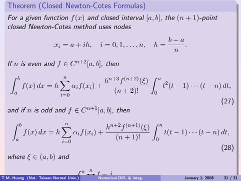
Theorem (Closed Newton-Cotes Formulas)

For a given function f(x) and closed interval [a, b], the (n + 1)-pointclosed Newton-Cotes method uses nodes

xi = a + ih, i = 0, 1, . . . , n, h =b− a

n.

If n is even and f ∈ Cn+2[a, b], then∫ b

af(x) dx = h

n∑i=0

αif(xi) +hn+3f (n+2)(ξ)

(n + 2)!

∫ n

0t2(t− 1) · · · (t− n) dt,

(27)and if n is odd and f ∈ Cn+1[a, b], then∫ b

af(x) dx = h

n∑i=0


(n + 1)!

∫ n

0t(t− 1) · · · (t− n) dt,

(28)where ξ ∈ (a, b) and

αi =∫ n

0

n∏j=0

j 6=i

t− j

i− jdt, i = 0, 1, . . . , n. (29)

Consequently, the degree of accuracy is n + 1 when n is an even integer,and n when n is an odd integer.


師大

The weights αi in the Newton-Cotes formula has the property

n∑i=0

αi = n. (30)

This can be shown by applying the formula to f(x) = 1 with interpolatingpolynomial Pn(x) = 1. Let s be the common denominator of αi, that is,

αi =σi

s(⇒ σi = sαi)

such that σi are integers, then the formulation for approximating thedefinite integral can be expressed as

∫ b

af(x) dx ≈ h

n∑i=0

αif(xi) =h

s

n∑i=0

σif(xi). (31)

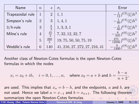
Some of the most common closed Newton-Cotes formulas with their errorterms are listed in the following table.


師大

Name n s σi Error

Trapezoidal rule 1 2 1, 1 − 112f (2)(ξ)h3

Simpson’s rule 2 3 1, 4, 1 − 190f (4)(ξ)h5

3/8-rule 3 83 1, 3, 3, 1 − 3

80f (4)(ξ)h5

Milne’s rule 4 452 7, 32, 12, 32, 7 − 8

945f (6)(ξ)h7

5 2885 19, 75, 50, 50, 75, 19 − 275

12096f (6)(ξ)h7

Weddle’s rule 6 140 41, 216, 27, 272, 27, 216, 41 − 91400f (8)(ξ)h9

Another class of Newton-Cotes formulas is the open Newton-Cotesformulas in which the nodes

xi = x0 + ih, i = 0, 1, . . . , n, where x0 = a + h and h =b− a

n + 2,

are used. This implies that xn = b− h, and the endpoints, a and b, arenot used. Hence we label a = x−1 and b = xn+1. The following theoremsummarizes the open Newton-Cotes formulas.


師大

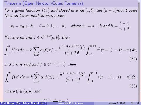
Theorem (Open Newton-Cotes Formulas)

For a given function f(x) and closed interval [a, b], the (n + 1)-point openNewton-Cotes method uses nodes

xi = x0 + ih, i = 0, 1, . . . , n, where x0 = a + h and h =b− a

n + 2.

If n is even and f ∈ Cn+2[a, b], then∫ b

af(x) dx = h

n∑i=0


(n + 2)!

∫ n+1

−1t2(t− 1) · · · (t− n) dt,

(32)and if n is odd and f ∈ Cn+1[a, b], then∫ b

af(x) dx = h

n∑i=0


(n + 1)!

∫ n+1

−1t(t− 1) · · · (t− n) dt,

(33)where ξ ∈ (a, b) and

αi =∫ n+1

−1

n∏j=0

j 6=i

t− j

i− jdt, i = 0, 1, . . . , n. (34)

Consequently, the degree of accuracy is n + 1 when n is an even integer,and n when n is an odd integer.


師大

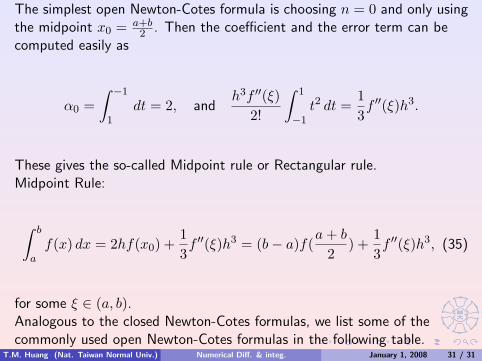
The simplest open Newton-Cotes formula is choosing n = 0 and only usingthe midpoint x0 = a+b

2 . Then the coefficient and the error term can becomputed easily as

α0 =∫ −1

1dt = 2, and

h3f ′′(ξ)2!

∫ 1

−1t2 dt =

13f ′′(ξ)h3.

These gives the so-called Midpoint rule or Rectangular rule.Midpoint Rule:

∫ b


13f ′′(ξ)h3 = (b− a)f(

a + b

2) +

13f ′′(ξ)h3, (35)

for some ξ ∈ (a, b).Analogous to the closed Newton-Cotes formulas, we list some of thecommonly used open Newton-Cotes formulas in the following table.


師大

Name n s σi Error

Midpoint rule 0 1 2 13f (2)(ξ)h3

1 2 3, 3 34f (2)(ξ)h3

2 3 8,−4, 8 1445f (4)(ξ)h5

3 24 55, 5, 5, 55 95144f (4)(ξ)h5

It is obvious that the Newton-Cotes formulas are generally not suitable fornumerical integration over large interval. Higher degree formulas would berequired, and the coefficients in these formulas are difficult to obtain. Alsothe Newton-Cotes formulas which are based on polynomial interpolationwould be inaccurate over a large interval because of the oscillatory natureof high-degree polynomials. Now we discuss a piecewise approach, calledcomposite rule, to numerical integration over large interval that uses thelow-order Newton-Cotes formulas.A composite rule is one obtained by applying an integration formula for asingle interval to each subinterval of a partitioned interval. To illustratethe procedure, we choose an even integer n and partition the interval [a, b]into n subintervals by nodes x0 < x1 < · · · < xn = b, and apply Simpson’s


師大

rule on each consecutive pair of subintervals. With

h =b− a

nand xj = a + jh, j = 0, 1, . . . , n,

we have on each interval [x2j−2, x2j ],

∫ x2j

x2j−2

f(x) dx =h

3[f(x2j−2) + 4f(x2j−1) + f(x2j)]−

h5

90f (4)(ξj),

for some ξj ∈ (x2j−2, x2j), provided that f ∈ C4[a, b]. The composite ruleT.M. Huang (Nat. Taiwan Normal Univ.) Numerical Diff. & integ. January 1, 2008 31 / 31

師大

is obtained by summing up over the entire interval, that is,∫ b

af(x) dx =

n/2∑j=1

∫ x2j

x2j−2

f(x) dx

=n/2∑j=1

[h

3(f(x2j−2) + 4f(x2j−1) + f(x2j))−

h5

90f (4)(ξj)

]=

h

3[f(x0) + 4f(x1) + f(x2) + f(x2) + 4f(x3) + f(x4) + f(x4) + 4f(x5)

+ · · ·+ f(xn−2) + 4f(xn−1) + f(xn)]− h5

90

n/2∑j=1

f (4)(ξj)

=h

3[f(x0) + 4f(x1) + 2f(x2) + 4f(x3) + 2f(x4) + 4f(x5)

+ · · ·+ 2f(xn−2) + 4f(xn−1) + f(xn)]− h5

90

n/2∑j=1

f (4)(ξj)

=h

3

f(x0) + 4n/2∑j=1

f(x2j−1) + 2(n/2)−1∑

j=1

f(x2j) + f(xn)

− h5

90

n/2∑j=1

f (4)(ξj).T.M. Huang (Nat. Taiwan Normal Univ.) Numerical Diff. & integ. January 1, 2008 31 / 31

師大

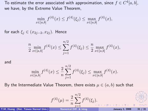
To estimate the error associated with approximation, since f ∈ C4[a, b],we have, by the Extreme Value Theorem,

minx∈[a,b]

f (4)(x) ≤ f (4)(ξj) ≤ maxx∈[a,b]

f (4)(x),

for each ξj ∈ (x2j−2, x2j). Hence

n

2min

x∈[a,b]f (4)(x) ≤

n/2∑j=1

f (4)(ξj) ≤n

2maxx∈[a,b]

f (4)(x),

and

minx∈[a,b]

f (4)(x) ≤ 2n

n/2∑j=1

f (4)(ξj) ≤ maxx∈[a,b]

f (4)(x).

By the Intermediate Value Theorem, there exists µ ∈ (a, b) such that

f (4)(µ) =2n

n/2∑j=1

f (4)(ξj).


師大

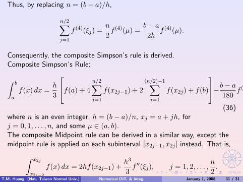
Thus, by replacing n = (b− a)/h,

n/2∑j=1

f (4)(ξj) =n

2f (4)(µ) =

b− a

2hf (4)(µ).

Consequently, the composite Simpson’s rule is derived.Composite Simpson’s Rule:

∫ b

af(x) dx =

h

3

f(a) + 4n/2∑j=1

f(x2j−1) + 2(n/2)−1∑

j=1

f(x2j) + f(b)

−b− a

180f (4)(µ)h4,

(36)where n is an even integer, h = (b− a)/n, xj = a + jh, forj = 0, 1, . . . , n, and some µ ∈ (a, b).The composite Midpoint rule can be derived in a similar way, except themidpoint rule is applied on each subinterval [x2j−1, x2j ] instead. That is,∫ x2j

x2j−2

f(x) dx = 2hf(x2j−1) +h3

3f ′′(ξj), j = 1, 2, . . . ,

n

2.


師大

Note that n must again be even. Consequently,∫ b

af(x) dx = 2h

n/2∑j=1

f(x2j−1) +h3

3

n/2∑j=1

f ′′(ξj).

The error term can be written as

n/2∑j=1

f ′′(ξj) =n

2f ′′(µ) =

b− a

2hf ′′(µ),

for some µ ∈ (a, b). Therefore, the composite Midpoint rule has thefollowing formulation.Composite Midpoint Rule:∫ b

af(x) dx = 2h

n/2∑j=1

f(x2j−1)−b− a

6f ′′(µ)h2, (37)

where n is an even integer, h = (b− a)/n, xj = a + jh, forj = 0, 1, . . . , n, and some µ ∈ (a, b).


師大

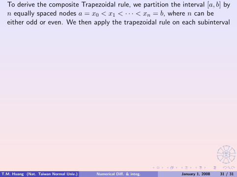
To derive the composite Trapezoidal rule, we partition the interval [a, b] byn equally spaced nodes a = x0 < x1 < · · · < xn = b, where n can beeither odd or even. We then apply the trapezoidal rule on each subinterval


師大

[xj−1, xj ] and sum them up to obtain

∫ b

af(x) dx =

n∑j=1

∫ xj

xj−1

f(x) dx

=n∑

j=1

[h

2(f(xj−1) + f(xj))−

h3

12f ′′(ξj)

]

=h

2[f(x0) + f(x1) + f(x1) + f(x2) + · · ·+ f(xn−1) + f(xn)]− h3

12

n∑j=1

f ′′(ξj)

=h

2[f(x0) + 2f(x1) + 2f(x2) + · · ·+ 2f(xn−1) + f(xn)]− h3

12

n∑j=1

f ′′(ξj)

=h

2

f(a) +n−1∑j=1

f(xj) + f(b)

− h3

12

n∑j=1

f ′′(ξj)

=h

2

f(a) +n−1∑j=1

f(xj) + f(b)

− b− a

12f ′′(µ)h2,


師大

where each ξj ∈ (xj−1, xj) and µ ∈ (a, b).Composite Trapezoidal Rule

∫ b

af(x) dx =

h

2

f(a) +n−1∑j=1

f(xj) + f(b)

− b− a

12f ′′(µ)h2, (38)

where n is an integer, h = (b− a)/n, xj = a + jh, for j = 0, 1, . . . , n, andsome µ ∈ (a, b).


numerical differentiation and...

Documents