numerical evidence on the uniform distribution of …hatleyj/involve-numerical-print.pdf ·...

inv lvea journal of mathematics

mathematical sciences publishers

2009 Vol. 2, No. 3

Numerical evidence on the uniform distribution ofpower residues for elliptic curves

Jeffrey Hatley and Amanda Hittson

INVOLVE 2:3(2009)

Numerical evidence on the uniform distribution ofpower residues for elliptic curves

Jeffrey Hatley and Amanda Hittson

(Communicated by Nigel Boston)

Elliptic curves are fascinating mathematical objects which occupy the intersec-tion of number theory, algebra, and geometry. An elliptic curve is an algebraicvariety upon which an abelian group structure can be imposed. By consideringthe ring of endomorphisms of an elliptic curve, a property called complex mul-tiplication may be defined, which some elliptic curves possess while others donot. Given an elliptic curve E and a prime p, denote by Np the number of pointson E over the finite field Fp. It has been conjectured that given an elliptic curveE without complex multiplication and any modulus M , the primes for whichNp is a square modulo p are uniformly distributed among the residue classesmodulo M . This paper offers numerical evidence in support of this conjecture.

1. Introduction

Let F(x, y)= y2−a1xy−a3 y− x3

−a2x2+a4x−a6 where the ai ∈C. Consider

the set of pointsE = {(x, y) ∈ C2

: F(x, y)= 0}.

We also wish to associate with the set E a special point O∈ E , called the point at in-finity, an idea which is made rigorous by projective geometry and whose existenceis justified below. Provided there are no points (x, y) such that

∂F∂x

∣∣∣∣(x,y)=∂F∂y

∣∣∣∣(x,y)= 0,

we say that F is nonsingular, and when F is nonsingular, we call E an ellipticcurve. Through some substitutions, the equations defining elliptic curves can beput into the form F(x, y) = y2

− x3− ax − b for some a, b ∈ C, which is called

Weierstrass normal form.

MSC2000: 11Y99.Keywords: elliptic curve, power residue, uniform distribution, computational algebraic geometry.This research was sponsored by grant number NSF-DMS 0552577 and the REU program, while theauthors were undergraduates at the College of New Jersey (Hatley) and Bryn Mawr College (Hittson).

305

306 JEFFREY HATLEY AND AMANDA HITTSON

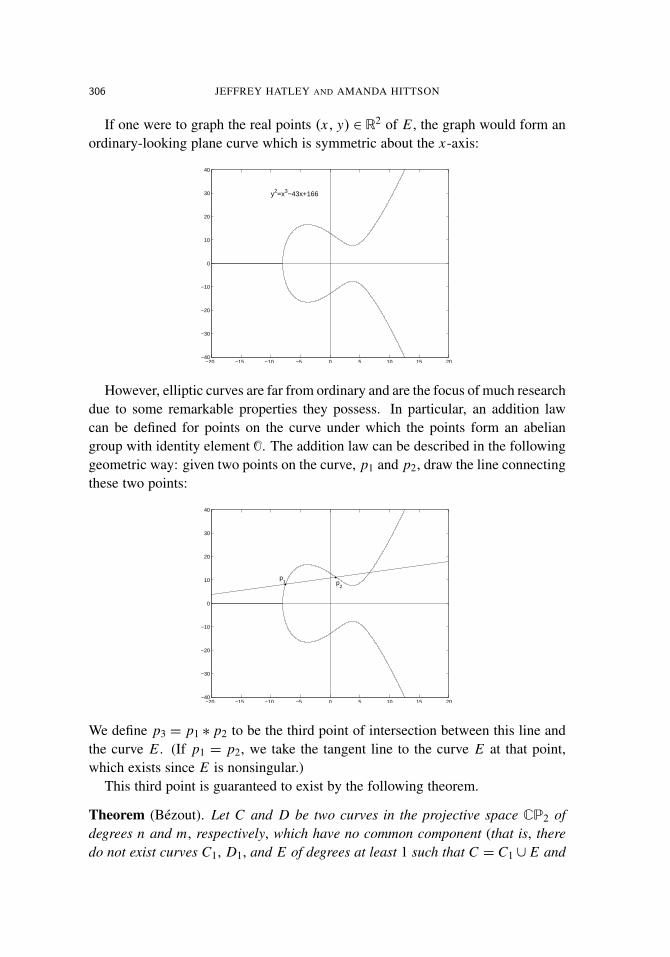
If one were to graph the real points (x, y) ∈ R2 of E , the graph would form anordinary-looking plane curve which is symmetric about the x-axis:

−20 −15 −10 −5 0 5 10 15 20−40

−30

−20

−10

0

10

20

30

40

y2=x3−43x+166

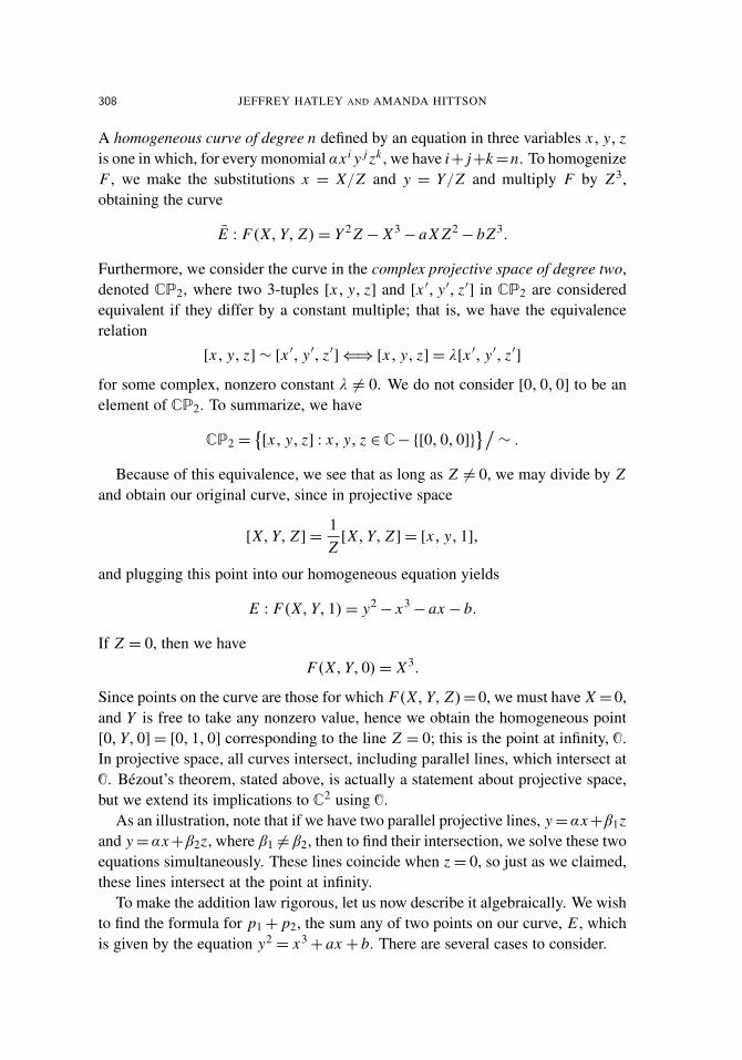
However, elliptic curves are far from ordinary and are the focus of much researchdue to some remarkable properties they possess. In particular, an addition lawcan be defined for points on the curve under which the points form an abeliangroup with identity element O. The addition law can be described in the followinggeometric way: given two points on the curve, p1 and p2, draw the line connectingthese two points:

−20 −15 −10 −5 0 5 10 15 20−40

−30

−20

−10

0

10

20

30

40

•p

1•p

2

We define p3 = p1 ∗ p2 to be the third point of intersection between this line andthe curve E . (If p1 = p2, we take the tangent line to the curve E at that point,which exists since E is nonsingular.)

This third point is guaranteed to exist by the following theorem.

Theorem (Bézout). Let C and D be two curves in the projective space CP2 ofdegrees n and m, respectively, which have no common component (that is, theredo not exist curves C1, D1, and E of degrees at least 1 such that C = C1 ∪ E and

UNIFORM DISTRIBUTION OF POWER RESIDUES FOR ELLIPTIC CURVES 307

D = D1 ∪ E). Then C and D have precisely nm points of intersection countingmultiplicities.

This theorem is about curves in projective space; projective space and its rolein the study of elliptic curves is discussed below. For a detailed discussion ofprojective space, multiplicity, and Bezout’s theorem, see [Kirwan 1992].

Bezout’s theorem states that two algebraic curves of degrees n and m intersectin exactly nm points (counting multiplicity), provided the curves do not share acommon component. Now, the degree of a curve is simply the degree of the homo-geneous polynomial defining it. (Homogeneous polynomials are discussed below.)Since E is defined by a polynomial of degree 3, E is of degree 3, and since a lineis of degree 1, Bezout’s theorem implies that the two curves should intersect inexactly 3 points; hence precisely one such point p3 is guaranteed to exist. Thenp1+ p2 is defined to be the reflection of p3 about the x-axis:

−20 −15 −10 −5 0 5 10 15 20−40

−30

−20

−10

0

10

20

30

40

•p

1•p

2

•p1*p

2

•p1+p

2

This method of addition is frequently referred to as the chord and tangent method.This addition law can be stated succinctly in the following way: three points on Esum to the identity, O, if and only if they are collinear. With this formulation, andthe understanding that O exists “at the top of the y-axis” as discussed below, wesee that p1 ∗ p2 = −(p1 + p2), and the reflection of this point across the y-axis,which we defined to be p1+ p2, is the third point of E on the line between p1 ∗ p2

and O.It is now necessary to consider O, the point at infinity. For our purposes, it

suffices to think of O as the point at which all vertical lines in the x − y planeintersect. Consider the line connecting p1 ∗ p2 and p1+ p2. This is a vertical line,and clearly only intersects E twice. However, Bezout’s Theorem assures us thatthere are three points of intersection. In this case, that third point is O.

To make this more rigorous, we consider the homogenized form of the curve Edefined by

E : F(x, y)= y2− x3− ax − b.


A homogeneous curve of degree n defined by an equation in three variables x, y, zis one in which, for every monomial αx i y j zk , we have i+ j+k=n. To homogenizeF , we make the substitutions x = X/Z and y = Y/Z and multiply F by Z3,obtaining the curve

E : F(X, Y, Z)= Y 2 Z − X3− aX Z2

− bZ3.

Furthermore, we consider the curve in the complex projective space of degree two,denoted CP2, where two 3-tuples [x, y, z] and [x ′, y′, z′] in CP2 are consideredequivalent if they differ by a constant multiple; that is, we have the equivalencerelation

[x, y, z] ∼ [x ′, y′, z′] ⇐⇒ [x, y, z] = λ[x ′, y′, z′]

for some complex, nonzero constant λ 6= 0. We do not consider [0, 0, 0] to be anelement of CP2. To summarize, we have

CP2 ={[x, y, z] : x, y, z ∈ C−{[0, 0, 0]}

}/∼ .

Because of this equivalence, we see that as long as Z 6= 0, we may divide by Zand obtain our original curve, since in projective space

[X, Y, Z ] =1Z[X, Y, Z ] = [x, y, 1],

and plugging this point into our homogeneous equation yields

E : F(X, Y, 1)= y2− x3− ax − b.

If Z = 0, then we have

F(X, Y, 0)= X3.

Since points on the curve are those for which F(X, Y, Z)= 0, we must have X = 0,and Y is free to take any nonzero value, hence we obtain the homogeneous point[0, Y, 0] = [0, 1, 0] corresponding to the line Z = 0; this is the point at infinity, O.In projective space, all curves intersect, including parallel lines, which intersect atO. Bezout’s theorem, stated above, is actually a statement about projective space,but we extend its implications to C2 using O.

As an illustration, note that if we have two parallel projective lines, y=αx+β1zand y=αx+β2z, where β1 6=β2, then to find their intersection, we solve these twoequations simultaneously. These lines coincide when z = 0, so just as we claimed,these lines intersect at the point at infinity.

To make the addition law rigorous, let us now describe it algebraically. We wishto find the formula for p1+ p2, the sum any of two points on our curve, E , whichis given by the equation y2

= x3+ ax + b. There are several cases to consider.


CASE 1: Let p1 = (x1, y1) and p2 = (x2, y2), and suppose p1 6= p2 and neitherpoint is equal to O. To find p1+ p2, we must first find p1 ∗ p2 = p3 = (x3, y3), thethird point of intersection of the line between p1 and p2 with E . The line betweenp1 and p2 is given by

y = λx + ν, where λ=y2− y1

x2− x1and ν = y1− λx1.

Now, we wish to find the points where this line intersects our curve, so we makethe following substitution:

y2= (λx + ν)2 = x3

+ ax + b.

Subtracting gives us

0= x3− λ2x2

+ (a− 2λ)x + (b− ν2).

The x-coordinates of the three points of intersection of the line and E are given bythe roots of this equation. Factoring, we obtain

x3− λ2x2

+ (a− 2λ)x + (b− ν2)= (x − x1)(x − x2)(x − x3),

and by identifying coefficients, we know that the sum of the roots is equal to thenegative of the coefficient of x2; that is,

x1+ x2+ x3 = λ2⇒ x3 = λ

2− x1− x2.

By the equation of our line, this allows us to find y3:

y3 = λx3+ ν.

Thus, we have p3 = (x3, y3). Now, the definition of our group law tells us thatsince p1, p2, and p3 are collinear, their sum must be equal to the group identity,which is O. Thus

p1+ p2+ p3 = O.

But this implies that p3 =−(p1+ p2). By the definition of the inverse of a groupelement, we know that

(p1+ p2)+ p3 = (p1+ p2)− (p1+ p2)= O.

Using the definition of our group law again, as well as the fact that O is the identityelement, we see that

(p1+ p2)+ p3+O= O,

which, geometrically, means that p1 + p2 is the third point of intersection of Ewith the line between p3 and O; but by our definition of O, this is just a vertical


line, and since E is symmetric about the x-axis, we conclude that p1+ p2 is simplythe reflection of p3 about the x-axis. Thus,

p1+ p2 =−p3 = (x3,−y3),

where x3 and y3 are given by

x3 = λ2− x1− x2, y3 = λx3+ ν. (1)

CASE 2: Let p1 = p2 = (x1, y1) 6= O. Then the line “connecting” p1 and p2 issimply the line tangent to E at p1. Since E is given by

y2= x3+ ax + b,

implicit differentiation yields

∂y∂x=

3x2− a

2y.

Then the formulas in (1) hold, by the exact same arguments, with λ= ∂y/∂x . Notethat λ blows up if y = 0; that is, the tangent line is vertical. So if p = (x, 0), thenp + p = 2p = O. Thus, the points of order two on E are precisely those withy-coordinate equal to zero.

CASE 3: If p1 = O, then since O is the identity element of the group, we have

p1+ p2 = O+ p2 = p2.

As an example, consider the curve E defined by

E = {(x, y) ∈ C2: y2= x3+ 17}.

It is easy to check that the points p1 = (2, 5) and p2 = (−1, 4) are on the curve.Applying the addition formulas given above, we see that λ= 1

3 , ν = 133 , and p1+

p2 = (−89 ,

10927 ), which is also easily verified to be on the curve.

To summarize, under the chord-and-tangent addition law and the inclusion ofO, E forms an abelian group with identity element O, where p1 + p2 + p3 = O ifand only if p1, p2, p3 ∈ E are the three points of intersection of some line with E .A wonderful introduction to elliptic curves can be found in [Silverman and Tate1992].

Frequently, one prefers to look at the set

E(Q)= {(x, y) ∈Q2: y2= x3+ ax + b with a, b ∈Q} ∪ {O}

of rational points on the curve. Here again, O is the point at infinity with projectivecoordinates O = [0, 1, 0], and under the chord-and-tangent method of addition,the algebraic description of which is given in (1), E(Q) forms an abelian groupwith identity element O. In fact, this is a subgroup of the original group E , and


interestingly, the Mordell–Weil theorem tells us that it is finitely-generated. Moregenerally, given a field K , one might look at the group

E(K )= {(x, y) ∈ K 2: y2= x3+ ax + b with a, b ∈ K } ∪ {O}

of K -rational points on the curve. Once again, O= [0, 1, 0] is the point at infinity.If K = Fp is the finite field with p elements, where p is an odd prime, then E(K )is called the reduction modulo p of E . An examination of our derivation of thealgebraic formulas for the addition law, given in (1), reveals that the formulas holdin any field, provided the field has characteristic other than 2. Under this additionlaw, E(K ) forms an abelian group with identity element O.

Let p be an odd prime. Given an elliptic curve E reduced modulo p, it iscommon to ask how many points Np lie on the curve (equivalently, what the orderis of the group given by the curve). Clearly this number is finite, since for each ofthe p possible values of x there are only two possible values of y, plus the pointat infinity O; hence there are at most 2p+1 points on the curve. A better estimatefor Np might be derived in the following way. An element a of Fp is said to be aquadratic residue if there exists a nonzero b ∈ Fp such that b2

≡ a (mod p). In Fp,there are exactly (p−1)/2 quadratic residues. Finding points (x, y) on E amountsto finding those values of x such that x3

+ax+b is a quadratic residue modulo p;hence we might expect x3

+ax+b to be a square modulo p about half of the time.Since each such square yields the two pairs (x, y) and (x,−y), we should expectabout p− 1 such points. We might also have x3

+ ax + b = 0, in which case weget the point (x, 0). Finally, there is the point at infinity. Adding these points up,we get an estimate of Np = p+ 1. Of course, this is a heuristic argument, so weshould expect an error term. A theorem due to Hasse and Weil bounds this errorterm:

Theorem (Hasse, Weil). If E is an elliptic curve defined over the finite field Fp,then the number of points on E with coordinates in Fp is p + 1− ap, where the“error term” ap satisfies |ap| ≤ 2

√p.

Returning to our previous example, let us look at the curve

E = {(x, y) ∈ F5 : y2= x3+ 2}.

In this case, brute force suffices to show that

E = {(2, 0), (3, 2), (3, 3), (4, 1), (4, 4),O},

hence Np = 6. Since p + 1 = 6, the error term from the Hasse–Weil theorem isin this case ap = 0, and our heuristic argument gave us Np exactly. This does nothappen in general, however.


In this paper, we are particularly interested in the set

QE = {odd primes p ∈ Z : Np is a quadratic residue modulo p}.

We have just shown that for the elliptic curve E which we have been considering,N5= 6≡ 1≡ 12 (mod 5), so 5∈ QE . Note that, in general, for two different curvesE1 and E2 we have QE1 6= QE2 .

Recall that an endomorphism of a group G is a homomorphismφ : G → G. Now, since an elliptic curve E/C defined over C forms a group, itis natural to study End(E), the ring of endormorphisms of E . (To be precise, weactually only look at rational endomorphisms, those which are defined by rationalfunctions with entries in C. These are also called isogenies.) For each integer n,the multiplication-by-n map φn : E → E defined by φn(x, y) = n(x, y) (wheren(x, y) represents repeated chord-and-tangent addition) defines an endomorphismof E , hence φn ∈ End(E). For most curves, these are the only endomorphisms;however, some curves do have additional endormorphisms, and these curves aresaid to have complex multiplication, or simply CM. Curves for which End(E)∼= Z

are said to be non-CM.Returning to our example curve E defined by the polynomial

y2= x3+ 17,

let φ : E→ E be the homomorphism defined by

φ(x, y)=(−1+

√−3

2x,−y

).

This is not a multiplication-by-n map, and since (−1+√−3

2 )3 = 1 and (−y)2 = y, if(x, y) ∈ E then also φ(x, y) ∈ E ; hence E has CM.

Conjecture. Let E be a non-CM curve, fix a modulus M , and let r1, . . . , rs denotethe residue classes modulo M such that gcd(ri ,M) = 1 for each i . Now, look atthe reduction of E modulo p for each p in the set Pn = {3, 5, . . . , pn} of the first nodd primes, calculate Np for each p, and let QE be defined as before. Let

Ri = {p ∈ QE ∩ Pn | p ≡ ri (mod M)}.

Let #Ri denote the cardinality of this set. Then the residues of the elements of QE

modulo M are uniformly distributed among the ri ; that is, for every 1≤ i, k ≤ s wehave

limn→∞

#Ri

#R j= 1.

This conjecture, suggested to Martin by Ramakrishna, is based on [Weston2005], which investigates a similar problem involving the distribution of powerresidues for ap ≡ Np − 1 (mod p).


To test this conjecture, we wrote a program using William Stein’s project Sagewhich takes as input an elliptic curve E , a range of moduli M , and a large numberB. For each modulus M , the program looks at the reduction of E modulo p forevery prime p < B and computes the number of points Np on the reduced ellipticcurve. Finally, it takes those p such that Np is a quadratic residue modulo p andlooks at their residues modulo M . The output data consists of 1) the number ofprimes congruent to ri for each residue class ri relatively prime to M , and 2) themaximum percent deviation of the size of each #Ri from the expected size (werethe Np distributed uniformly among the ri ).

In this paper, we present data from our program for several curves without CM,arguing that the trends in the data as B increases strongly suggest the truth of theconjecture.

2. The program

2.1. What the programs do. To get the data we needed, we wrote a program thattakes an elliptic curve and a few other parameters, computes a subset of the primenumbers, called QE , and, given a modulus M , computes a count for each residue.The count is the number of elements in QE that, when reduced modulo M , havethat residue. The program also computes the largest percent difference from theexpected value.

More specifically, given an elliptic curve E , a range of prime numbers P , and arange of moduli M , the program computes the set

QE = {p ∈ P | Np is a quadratic residue modulo p}.

Then for all m ∈ M , the program computes for each residue r ,

#R = #{p ∈ P | p ≡ r (mod m)}.

This information is written to a file. Then the program computes some statisticalinformation. First, it computes the expected count for each residue. If a residue, r ,is not relatively prime to the modulus, m, then p ∈ QE will have p≡ r (mod m)⇔r ∈ QE . This means that #R = 0, 1 for all residues, r , that are not relatively primeto m. So we are really only interested in residues relatively prime to the modulus.If the conjecture were true for non-CM elliptic curves, we would expect that

#Ri =#QE

ϕ(m),

where ϕ(m) = #{r ∈ Z | 0 ≤ r < m and gcd(r,m) = 1} denotes the Euler-phifunction and r1, . . . , rs are the residues relatively prime to m. For each modulus,m, the program computes the percent difference of the actual count, #Ri , from theexpected count, C = (#QE)/ϕ(m). So the percent difference for each residue is


|1− #Ri/C | · 100. The program then picks out the largest percent difference. Weare interested in the largest percent difference because it tells us how far off theactual count is from the expected count. Finally, the program writes to a file eachmodulus and its corresponding largest percent difference.

For example, consider the elliptic curve E defined by

F(x, y)= y2+ xy+ y− x3

− 4x + 6.

Then given

P = {p ∈ Z+ | p < 106, p prime},

M = {m ∈ Z | 3≤ m < 301}, and

QE = {p ∈ P | Np is a quadratic residue modulo p},

the program computed that #QE = 40593. Now consider a specific modulus, saym = 9. Then the residues relatively prime to m are r1 = 1, r2 = 2, r3 = 4, r4 =

5, r5 = 7, r6 = 8, so ϕ(m)= 6. Thus the expected count for each residue is

C =#QE

ϕ(m)=

405936= 6765.5.

In fact, the program computed that the actual counts are

#R1 = 6551, #R2 = 6876, #R3 = 6802,

#R4 = 6850, #R5 = 6632, #R6 = 6882.

So there are 6551 primes p less than one million such that Np is a quadraticresidue modulo p and p ≡ 1 (mod 9). In fact, of these six counts, #R1 is thefarthest off from the expected count C = 6765.5. So #R1 will yield the biggestpercent difference, which is ∣∣∣1− #R1

C

∣∣∣ · 100≈ 3.17.

2.2. Outline of programs and efficiency. We organized the programs to try tomaximize efficiency. The original programs we wrote were slow. Using them,we could not have computed nearly the same amount of data that we did withour newer version. By timing the original programs, we were able to see that theprocess that took the most time was generating and storing the set QE . Since thisset was not even an output of our programs, we decided to generate one part ofQE at a time. It worked like this:

while counter < limit:compute part of QE beginning with counterread in previously computed data (if any)compute counts for this part of QE


save these datadelete current part of QE

compute percentages for all data

Note that counter and limit are simply variables to keep track of which piece ofQE has been computed.

This while loop lends itself to division into two programs: 1) a program to returna part of the set QE and 2) a program to maintain a count of the residue classesin the set QE over the various moduli in some set M . After running initial testson various curves for primes strictly less than one hundred thousand, which ran inunder five minutes, and then for primes strictly less than one million, which ran formore than two hours, we realized that the second run of these tests was recomputingdata. This led us to modify the second program to look for output files generatedby previous runs of the program and start with an updated count and then proceedfrom there. This also meant that if the program crashed in the middle of running,we wouldn’t lose all previous data. Finally, there are several driver programs thatrun the tests for various elliptic curves, various ranges of moduli and various rangesof prime numbers.

2.3. How the main programs work. The main program, called residueCounter, isthe second program described in the preceding paragraph. It takes as parametersa starting number and upper bound to specify which range of prime integers tolook at, a starting modulus and ending modulus to specify which range of modulito test, a list of five integers to specify an elliptic curve, and finally a boolean tospecify whether or not to look for files containing data that this program can use.The program stores all of the output in a dictionary, called dataDict. The keys ofthe dictionary are the moduli in the range specified by the parameters. Given amodulus, m, dataDict[m] evaluates to a list of lists. This list is a count for eachresidue of m.

The program starts by deciding whether or not to look for old files based on theboolean passed as a parameter.

if True:find all files generated by previous runs of residueCounterpick the most relevant fileinitialize dataDict to include all of the data computed from this fileexclude the primes already checked by this file

if False:initialize a blank dataDict

Note that the most relevant file is the file whose range of moduli match that ofthe current program and of the files whose ranges match; the one with the highestupper bound has the most data and hence will save the most time.


The program needs to find the set QE and update dataDict to include the countfrom this set. However, as mentioned in the previous section, the program runstoo slowly to do this all at once. So, instead it runs a loop that calls a differentfunction, the first one mentioned above, to return a piece of QE , update dataDictto get all the counts for this piece, and then repeat this over and over until dataDicthas all the data needed.

More precisely, the program has a variable current prime to keep track of whatpart of QE has been retrieved. It then runs the following while loop:

while current prime is strictly less than the upper bound:call functionthis function returns a new current prime and a piece of QE

update dataDict for this piece of QE

get rid of that piece of QE to clear up memory spacetry to run loop again

The program then calculates the largest percent difference for each modulus, asdescribed in Section 2.1. Finally, it writes this information to two different files,one for the data, one for the statistical information. The file names are keyed toinclude the elliptic curve, the upper bound, the range of moduli and what kind offile it is.

The function called in the last while loop is the one that actually deals with theelliptic curves. The elliptic curves we are looking at have the form y2

+ a1xy +a3 y = x3

+a2x2+a4x +a5 for some a1, a2, a3, a4, a6 ∈ Z. This way we can look

at the curves reduced modulo p for odd primes p. A standard way to reference aspecific curve is by a list of the coefficients [a1, a2, a3, a4, a6].

This function takes as parameters an elliptic curve in the form [a1, a2, a3, a4, a6],the current prime, how many primes to check and the upper bound. It then calcu-lates the conductor of the elliptic curve. Every elliptic curve has a unique integerassociated with it, called the conductor. Essentially, the conductor tells you whichprimes to avoid; every prime divisor of the conductor has what is known as ‘badreduction’, meaning that the reduction of E modulo these primes is singular andtherefore not an elliptic curve. Accordingly, this function skips all of these primes.Also, we are only interested in primes p such that Np is a quadratic residue modulop. Luckily, there is a quick way to find out if Np is a quadratic residue. A result dueto Euler says that a necessary and sufficient condition for a ∈ Fp to be a quadraticresidue is:

a(p−1)/2≡ 1 (mod p).

The numbers Np are calculated in Sage via the command cardinality usingeither the Schoof–Elkies–Atkins algorithm or the baby-step-giant-step algorithm


of Mestre and Shanks. Sage decides which algorithm to use by heuristically deter-mining which will be more computationally efficient.

That said, here is a sketch of the program:

compute conductor of elliptic curveinitialize blank list to store primes of interestwhile (current prime < upper bound) and (counter < how many primes to check):

if current prime doesn’t divide conductor:if the coefficients define an elliptic curve:

if N (p−1)/2p ≡ 1 (mod p):

add current prime to listset current prime to the next prime

3. The data

Let us recall the conjecture on which we are working.

Conjecture. Given a non-CM elliptic curve E , a modulus M , and a list QE ofall the primes p for which the number of points Np on the reduction of E modulop are quadratic residues modulo p, the elements of QE are uniformly distributedamong the residue classes of M.

Due to the nature of the conjecture, the data we collect is bound to have someexperimental error, since we can only look at a finite subset of QE at a time. Whenthis subset of QE is large with respect to the modulus M , we should expect lesserror, and when this subset is small with respect to M , we should expect greatervariance in the distribution of the primes, and hence greater error.

When we ran our program, to obtain our subset of QE we took all of the primesin QE below some fixed bound B. We then looked at their distribution amongthe residue classes of moduli from 3 to 300. The preceding discussion suggeststhat by increasing the size of B, we should expect to see our experimental errordecrease. Consider Figure 1, which shows the data for F(x, y)= y2

+ y−x3+x , a

curve lacking complex multiplication. The bars in the graph indicate the maximum

0 50 100 150 200 250 3000

10

20

30

40

50

60

70

80

moduli

larg

est p

erce

nt d

iffer

ence

B = 105

0 50 100 150 200 250 3000

10

20

30

40

50

60

70

80

moduli

larg

est p

erce

nt d

iffer

ence

B = 106

0 50 100 150 200 250 3000

10

20

30

40

50

60

70

80

moduli

larg

est p

erce

nt d

iffer

ence

B = 3× 106

Figure 1. Prime distribution on the non-CM curve y2+y= x3

−xof conductor 37 and rank 1, for different values of the bound B.


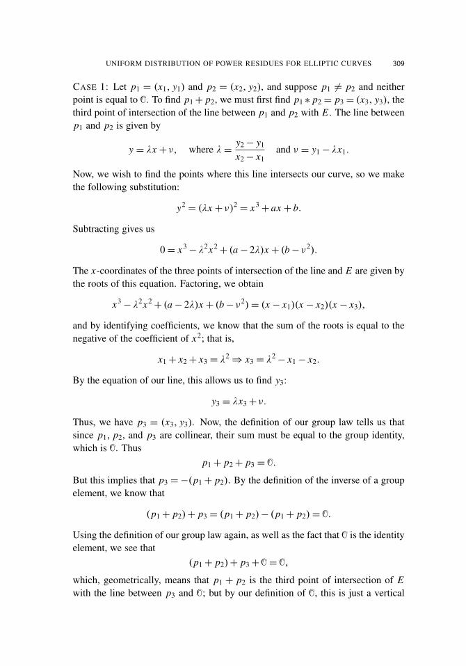
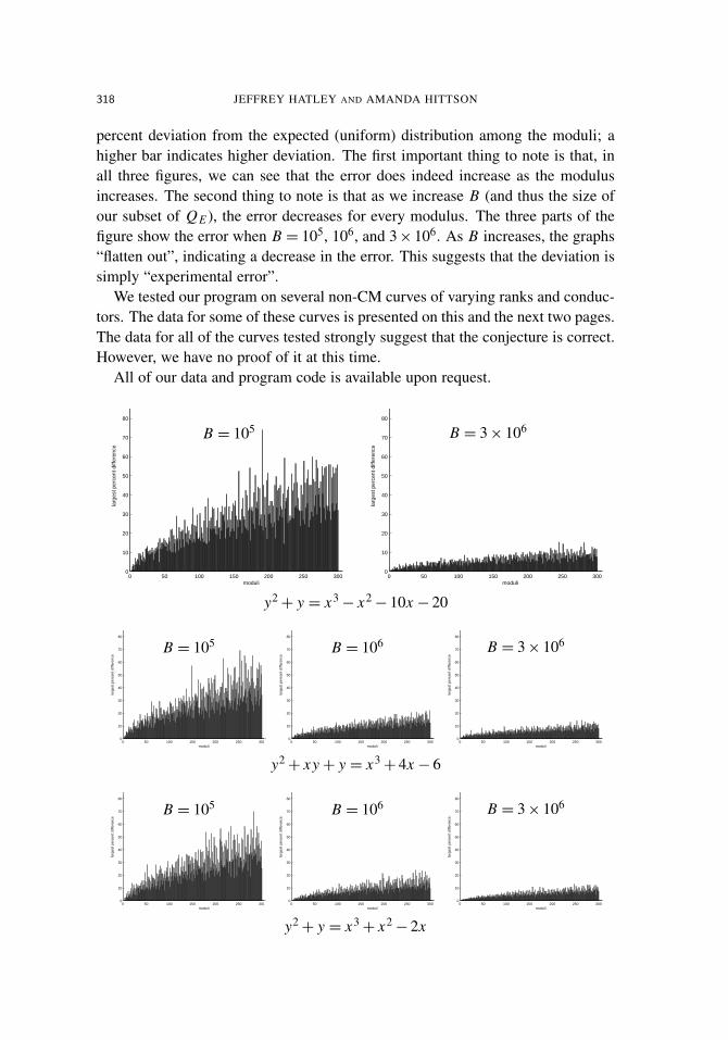
percent deviation from the expected (uniform) distribution among the moduli; ahigher bar indicates higher deviation. The first important thing to note is that, inall three figures, we can see that the error does indeed increase as the modulusincreases. The second thing to note is that as we increase B (and thus the size ofour subset of QE ), the error decreases for every modulus. The three parts of thefigure show the error when B = 105, 106, and 3×106. As B increases, the graphs“flatten out”, indicating a decrease in the error. This suggests that the deviation issimply “experimental error”.

We tested our program on several non-CM curves of varying ranks and conduc-tors. The data for some of these curves is presented on this and the next two pages.The data for all of the curves tested strongly suggest that the conjecture is correct.However, we have no proof of it at this time.

All of our data and program code is available upon request.

0 50 100 150 200 250 3000

10

20

30

40

50

60

70

80

moduli

larg

est p

erce

nt d

iffer

ence

B = 105

0 50 100 150 200 250 3000

10

20

30

40

50

60

70

80

moduli

larg

est p

erce

nt d

iffer

ence

B = 3× 106

y2+ y = x3

− x2− 10x − 20

0 50 100 150 200 250 3000

10

20

30

40

50

60

70

80

moduli

larg

est p

erce

nt d

iffer

ence

B = 105

0 50 100 150 200 250 3000

10

20

30

40

50

60

70

80

moduli

larg

est p

erce

nt d

iffer

ence

B = 106

0 50 100 150 200 250 3000

10

20

30

40

50

60

70

80

moduli

larg

est p

erce

nt d

iffer

ence

B = 3× 106

y2+ xy+ y = x3

+ 4x − 6

0 50 100 150 200 250 3000

10

20

30

40

50

60

70

80

moduli

larg

est p

erce

nt d

iffer

ence

B = 105

0 50 100 150 200 250 3000

10

20

30

40

50

60

70

80

moduli

larg

est p

erce

nt d

iffer

ence

B = 106

0 50 100 150 200 250 3000

10

20

30

40

50

60

70

80

moduli

larg

est p

erce

nt d

iffer

ence

B = 3× 106

y2+ y = x3

+ x2− 2x


0 50 100 150 200 250 3000

10

20

30

40

50

60

70

80

moduli

larg

est p

erce

nt d

iffer

ence

B = 105

0 50 100 150 200 250 3000

10

20

30

40

50

60

70

80

moduli

larg

est p

erce

nt d

iffer

ence

B = 106

y2+ y = x3

− 7x + 6

0 50 100 150 200 250 3000

10

20

30

40

50

60

70

80

moduli

larg

est p

erce

nt d

iffer

ence

B = 105

0 50 100 150 200 250 3000

10

20

30

40

50

60

70

80

moduli

larg

est p

erce

nt d

iffer

ence

B = 106

y2+ xy = x3

− x2− 79x + 289

0 50 100 150 200 250 3000

10

20

30

40

50

60

70

80

moduli

larg

est p

erce

nt d

iffer

ence

B = 105

0 50 100 150 200 250 3000

10

20

30

40

50

60

70

80

moduli

larg

est p

erce

nt d

iffer

ence

B = 106

y2+ y = x3

− 79x + 342

0 50 100 150 200 250 3000

10

20

30

40

50

60

70

80

moduli

larg

est p

erce

nt d

iffer

ence

B = 105

0 50 100 150 200 250 3000

10

20

30

40

50

60

70

80

moduli

larg

est p

erce

nt d

iffer

ence

B = 106

y2+ xy = x3

+ x2− 2582x + 48720


0 50 100 150 200 250 3000

10

20

30

40

50

60

70

80

moduli

larg

est p

erce

nt d

iffer

ence

B = 105

0 50 100 150 200 250 3000

10

20

30

40

50

60

70

80

moduli

larg

est p

erce

nt d

iffer

ence

B = 106

y2= x3− 10012x + 346900

0 50 100 150 200 250 3000

10

20

30

40

50

60

70

80

moduli

larg

est p

erce

nt d

iffer

ence

B = 105

0 50 100 150 200 250 3000

10

20

30

40

50

60

70

80

moduli

larg

est p

erce

nt d

iffer

ence

B = 106

y2+ y = x3

− 23737x + 960366

0 50 100 150 200 250 3000

10

20

30

40

50

60

70

80

moduli

larg

est p

erce

nt d

iffer

ence

B = 105

0 50 100 150 200 250 3000

10

20

30

40

50

60

70

80

moduli

larg

est p

erce

nt d

iffer

ence

B = 106

y2+ y = x3

+ x2− 3529920x + 2567473020

4. Future research ideas

Several related problems might be considered in the future. It would be beneficialto find an efficient way to run a program like ours for larger primes for furtherdata collection. The data presented in is paper is for values of B at the limit ofour program’s reasonable run time. We plan to modify our program to test theconjecture regarding ap rather than Np; furthermore, Weston [2005] conjecturesthat a similar result holds for primes for which the ap are higher power residues. A


slight modification of our program, or any similar program, would allow for datacollection for these cases.

Acknowledgement

This work was completed at the James Madison University Summer 2008 REUProgram. We thank our mentor, Jason Martin, for all his help and guidance withthis project.

References

[Kirwan 1992] F. Kirwan, Complex algebraic curves, London Mathematical Society Student Texts23, Cambridge University Press, Cambridge, 1992. MR 93j:14025 Zbl 0744.14018

[Silverman and Tate 1992] J. H. Silverman and J. Tate, Rational points on elliptic curves, Springer,New York, 1992. MR 93g:11003 Zbl 0752.14034

[Weston 2005] T. Weston, “Power residues of Fourier coefficients of modular forms”, Canad. J.Math. 57:5 (2005), 1102–1120. MR 2006e:11058 Zbl 1105.11011

Received: 2008-09-21 Revised: 2009-04-01 Accepted: 2009-04-11

[email protected] Department of Mathematics, University of Massachusetts,Amherst, MA 01003-9305, United States

[email protected] Department of Mathematics, University of Wisconsin,480 Lincoln Drive, Madison, WI 53706-1388, United States

numerical evidence on the uniform distribution of …hatleyj/involve-numerical-print.pdf ·...

Documents