numerical heat transfer, part b: fundamentals numerical ...nht.xjtu.edu.cn/paper/en/2010208.pdf ·...

PLEASE SCROLL DOWN FOR ARTICLE

This article was downloaded by: [Tao, W. Q.][Xi'an Jiaotong University]On: 9 March 2010Access details: Access Details: [subscription number 917681058]Publisher Taylor & FrancisInforma Ltd Registered in England and Wales Registered Number: 1072954 Registered office: Mortimer House, 37-41 Mortimer Street, London W1T 3JH, UK

Numerical Heat Transfer, Part B: FundamentalsPublication details, including instructions for authors and subscription information:http://www.informaworld.com/smpp/title~content=t713723316

Numerical Illustrations of the Coupling Between the Lattice BoltzmannMethod and Finite-Type Macro-Numerical MethodsH. B. Luan a; H. Xu a; L. Chen a; D. L. Sun b; W. Q. Tao a

a State Key Laboratory of Multiphase Flow in Power Engineering, School of Energy & PowerEngineering, Xi'an Jiaotong University, Xi'an, Shaanxi, People's Republic of China b Beijing KeyLaboratory of New and Renewable Energy, North China Electric Power University, Beijing, People'sRepublic of China

Online publication date: 08 March 2010

To cite this Article Luan, H. B., Xu, H., Chen, L., Sun, D. L. and Tao, W. Q.(2010) 'Numerical Illustrations of the CouplingBetween the Lattice Boltzmann Method and Finite-Type Macro-Numerical Methods', Numerical Heat Transfer, Part B:Fundamentals, 57: 2, 147 — 171To link to this Article: DOI: 10.1080/15421400903579929URL: http://dx.doi.org/10.1080/15421400903579929

Full terms and conditions of use: http://www.informaworld.com/terms-and-conditions-of-access.pdf

This article may be used for research, teaching and private study purposes. Any substantial orsystematic reproduction, re-distribution, re-selling, loan or sub-licensing, systematic supply ordistribution in any form to anyone is expressly forbidden.

The publisher does not give any warranty express or implied or make any representation that the contentswill be complete or accurate or up to date. The accuracy of any instructions, formulae and drug dosesshould be independently verified with primary sources. The publisher shall not be liable for any loss,actions, claims, proceedings, demand or costs or damages whatsoever or howsoever caused arising directlyor indirectly in connection with or arising out of the use of this material.

http://www.informaworld.com/smpp/title~content=t713723316

http://dx.doi.org/10.1080/15421400903579929

http://www.informaworld.com/terms-and-conditions-of-access.pdf

NUMERICAL ILLUSTRATIONS OF THE COUPLINGBETWEEN THE LATTICE BOLTZMANN METHOD ANDFINITE-TYPE MACRO-NUMERICAL METHODS

H. B. Luan1, H. Xu1, L. Chen1, D. L. Sun2, and W. Q. Tao11State Key Laboratory of Multiphase Flow in Power Engineering, School ofEnergy & Power Engineering, Xi’an Jiaotong University, Xi’an, Shaanxi,People’s Republic of China2Beijing Key Laboratory of New and Renewable Energy, North ChinaElectric Power University, Beijing, People’s Republic of China

An analytic expression called a reconstruction operator is proposed for the exchange from

velocity of finite-type methods to the single-particle distribution function of the lattice

Boltzmann method (LBM). The combined finite-volume method and lattice Boltzmann

method (called the CFVLBM) is adopted to solve three flow cases, backward-facing flow,

flow around a circular cylinder, and lid-driven cavity flow. The results predicted by the

CFVLBM agree with the available numerical solutions very well. It is shown that the

vorticity contour distribution is a more appropriate parameter to ensure good smoothness

and consistency at the coupling interface. At the same time, CPU time used by the

CFVLBM(II), with more than one outer iteration before interface information exchange,

is much less than that of the CFVLBM(I), where interface information exchanges are

executed after each outer iteration.

1. INTRODUCTION

Challenging multiscale phenomena or processes exist widely in, for example,material science, fluid flows, and electrical and mechanical engineering [1–3]. Thingsare made up of atoms and electrons at the atomic scale, but they are usually severalorders of magnitude larger when they are characterized by their own geometricdimensions. The study of multiscale problems has become one of the highlights ofnumerical simulation techniques, and several international journals have beencreated in the past 10 years. Examples of multiscale problems include turbulent fluidflow and heat transfer, transport phenomena in the proton exchange membranes offuel cells, cooling processes in data centers, and so on. Multiscale problems can bedivided into two categories: multiscale systems and multiscale processes. By multi-scale system we refer to a system that is characterized by large variations in length

Received 25 September 2009; accepted 1 December 2009.

This work is supported by Key Project of the National Natural Science Foundation of China

No. 50636050.

Address correspondence to W. Q. Tao, State Key Laboratory of Multiphase Flow in Power

Engineering, School of Energy & Power Engineering, Xi’an Jiaotong University, 28 Xian Ning Road,

Xi’an, Shaanxi 710049, People’s Republic of China. E-mail: [email protected]

Numerical Heat Transfer, Part B, 57: 147–171, 2010

Copyright # Taylor & Francis Group, LLC

ISSN: 1040-7790 print=1521-0626 online

DOI: 10.1080/15421400903579929

147

Downloaded By: [Tao, W. Q.][Xi'an Jiaotong University] At: 01:02 9 March 2010

scales. The processes at different scales are not very closely related and can be studiedseparately with certain connections. Cooling in data centers is a typical multiscalesystem problem. The length scale of the cooling stream in the center as a whole is ofthe order of meters, while the cooling process of a chip is of the order of millimeters.By a multiscale process we mean that the overall behavior is governed by processes thatoccur at different length and=or time scales, and they are inherently connected by theprocess itself. Processes in PEMFC, launching a space rocket from the earth surfaceto outer space, and turbulent heat transfer are examples of multiscale process. Fromthe viewpoint of simulation, study of the multiscale processes is more challenging andattractive. The focus of the present article is therefore on the multiscale processes.

It is usually accepted that different scale problems have different numericalmethods which are most applicable to the corresponding scales. Broadly speaking,there are three levels of simulation methods for fluid flow and heat transfer: macro-scale, mesoscale, and microscale. The macroscale numerical methods include thefinite-difference method (FDM), the finite-volume method (FVM), the finite-elementmethod (FEM), and the finite analytic method (FAM) [4]. The basic feature of thefour methods is that the smallest unit for computation is a cell with finite dimensions.Thus they can be called finite-type methods. The mesoscale numerical methodsinclude the lattice Boltzmann method (LBM) and the direct-simulation Monte Carlomethod (DSMC). These two methods adopt a concept of computational particleswhich are much larger than actual molecules but act as molecules (simulation mole-cules). The micro numerical methods include molecular dynamic simulation (MDS)and quantum molecular simulation (QMS). In MDS, every molecule is simulatedaccording to Newton’s law of motion. A quantum molecular dynamics simulationsolves the coupled time-dependent Schrodinger equations for all particles in thesystem. This method is largely limited by present computer resources; hence, variousapproximations have to be used.

NOMENCLATURE

c lattice speed

cs lattice sound speed

C compression operator

CD drag coefficient

D2Q9 2-dimension, 9-velocity lattice

f lattice distribution function

H height

I identity operator

Kn Knudsen number

L reattachment length

Ma Mach number

p pressure

r cylinder radius

R reconstruction operator

Re Reynolds number

S stress tension, step height

t time

u, v velocities along the x, y directions

ulid lid-driven velocity

u1 far-field velocity

u0 inlet velocity

x, y Cartesian coordinates

Dx space step

Dt time step

e expanding parameter

h separation angle

k relaxation time

n kinematic viscosity

q density

s nondimensional relaxation time

x weight factor

Subscripts

i direction of the discretized velocity

a, b, c coordinate direction indices

Superscript

eq equilibrium

148 H. B. LUAN ET AL.


As indicated above, many engineering processes are multiscale in nature.However, mainly because of the limitation of computer resources; before theemergence of the new simulation field of ‘‘multiscale simulation,’’ the inherentlymultiscale processes were usually simulated by single-scale numerical methods.One exception is direct numerical simulation (DNS) for turbulent flow. Thenumerical methods used in DNS, such as finite difference or finite volume, areof macroscale type. However, since a very tiny time scale and a very fine spacescale have to be used in DNS, the time and space resolutions in DNS are fineenough to resolve eddies and fluctuations at different scales. Hence the numericalresults obtained by DNS include enormous instant and local information and areessentially in multiscale. Averaged parameters, such as time-averaged velocity, canbe obtained from the simulation results. Since DNS is not suitable for othermultiscale processes, the terminology of ‘‘multiscale simulation’’ is usually notused in reference to this method.

The other traditional numerical approaches for inherently multiscale problemsfocus on the scale of interest and eliminate the effects of other scales. As indicated in[1], such approaches have limitations. If we adopt a macroscale method to simulate amultiscale process, three limitations may occur: accuracy, lack of detail for somespecial process, and the necessity of introducing empirical closures. On the otherhand, if we use micro method—say, MDS—to simulate a multiscale process forthe entire geometric domain, the required computer resource is not realistic.

This is where multiscale modeling technique comes in. Here, multiscalemodeling implies a coupling technique in which some macro=meso=micro simula-tion methods are used in different local regimes for numerical simulations of thesame engineering problem. The macro numerical methods usually are finite-typemethods (FDM, FVM, FEM, or FAM). By mesoscale and microscale methodswe usually mean the LBM, DSMC, MDS, and QMS, respectively. In such a mul-tiscale simulation, the key issue is how to transfer information between twoneighboring regimes in order to guarantee numerical stability, accuracy, andefficiency of computations.

A very typical multiscale simulation was provided recently by Abraham [5],who applied three levels of simulation schemes, FEM-MDS-QMS, to study crackdynamics. Nie et al. [6] adopted the MDS and FVM for the lid-driven cavity flowin which the two vertexes are single point in math. Dupuis et al. [7] proposed anLB-MD model for simulations of flows of liquid argon past and through a carbonnanotube. Wu et al. [8] proposed a scheme of coupled DSMC-NS using an unstruc-tured mesh. The numerical approaches adopted in [5–8] have one thing in common:For the same problem, different regions are solved by different numerical methodsand the results are coupled at their interfaces. In this article, this approach is adoptedand the focus is on how to transfer information at the interface between the results ofthe LBM and those of the finite-type methods.

In the following, we first present a brief overview of the lattice Boltzmannmodel and the finite-volume model (Section 2). Then, we describe the basics andimplement procedures of the couple strategy (Section 3). After that, we employthis couple strategy to solve the backward-facing step flow, flow around a circularcylinder, and lid-driven cavity flow (Section 4). Finally, some conclusions aregiven.

ILLUSTRATIONS OF THE COUPLING BETWEEN LBM AND FVM 149


2. LATTICE BOLTZMANN MODEL AND FINITE-VOLUME MODEL

2.1. Lattice Boltzmann Model

The lattice Boltzmann method can be easily coupled to the finite-type methodsfor continuum partial differential equations, partly because of its small time stepsand geometric flexibility [2]. The LBM combines the power of continuum methodswith the geometric flexibility of the atomistic method, which is a bridge betweenmacroscale and microscale numerical methods. To play this bridge role the LBMshould be coupled downward with micro- and upward with macroscopic methods.Taking the upward coupling into consideration, the transfer of LBM results tomacro results is very easy. However, the transfer of macro results to the particledistribution function of the LBM is not straightforward. This article offers thedetails of coupling the macroscale results with the LBM results.

A popular kinetic model of the LBM adopted in the literature is thesingle-relaxation-time (SRT) approximation, the so-called Bhatnagar-Gross-Krook(BGK) model [9],

qfqt

þ c � rf ¼ � 1

kf � f ðeqÞ

� �ð1Þ

where f is the single-particle distribution function, rf is the gradient of the functionf, c is the particle velocity vector, f (eq) is the equilibrium distribution function (theMaxwell-Boltzmann distribution function), and k is the relaxation time.

To solve for f numerically, Eq. (1) is first discretized in the velocity spaceusing a finite set of velocities {ci} without affecting the conservation laws [10,11], giving

qfiqt

þ ci � rfi ¼ � 1

kfi � f

ðeqÞi

� �ð2Þ

In the above equation, fi(x, t)� f(x, ci, t) is the distribution function associated withthe ith discrete velocity ci, and f

ðeqÞi is the ith equilibrium distribution function. The

nine-velocity square lattice model D2Q9 [12] (Figure 1) has been used successfullyfor simulating 2-D flow. The nine velocities, denoted by ci, are given by

c0 ¼ 0

ci ¼ c cos i � 1ð Þp=4½ �; sin i � 1ð Þp=4½ �f g for i ¼ 1; 2; 3; 4

ci ¼ffiffiffi2

pc cos i � 1ð Þp=4½ �; sin i � 1ð Þp=4½ �f g for i ¼ 5; 6; 7; 8

ð3Þ

where c¼Dx=Dt, Dx is the lattice spacing step size, and Dt is the time-step size. Theequilibrium distribution function is given by

fðeqÞi ¼ xiq 1þ 3

c2ci � uð Þ þ 9

2c4ci � uð Þ2� 3

2c2u2

� �ð4Þ

with the weights x0¼ 4=9, x1¼x2¼x3¼x4¼ 1=9, x5¼x6¼x7¼x8¼ 1=36.



The macroscopic density q and velocity vector u can be evaluated as

q ¼X8i¼0

fi ð5aÞ

qu ¼X8i¼0

cifi ð5bÞ

The pressure of an ideal gas can be calculated from p ¼ qc2s , with the speed of soundbeing cs ¼ c=

ffiffiffi3

p. In the LBM, Eq. (2) is discretized in both time and space, and the

completely discretized equation (also the evolution equation) is

fi xþ ciDt; tþ Dtð Þ ¼ fi x; tð Þ � 1

sfi x; tð Þ � f

eqð Þi x; tð Þ

h ið6Þ

where s¼ k=Dt.Equation (6) can be divided into two substeps: (1) collision, which occurs when

particles at a node interact with each other and then change velocity directionsaccording to scattering rules; and (2) streaming, in which each particle moves tothe nearest node in the velocity direction.Collision step:

~ffi x; tð Þ ¼ fi x; tð Þ � 1

sfi x; tð Þ � f

ðeqÞi x; tð Þ

h ið7aÞ

Streaming step:

fi xþ ciDt; tþ Dtð Þ ¼ ~ff i x; tð Þ ð7bÞ

where ~ffi represents the postcollision state.

Figure 1. A 2-D, 9-velocity (D2Q9) lattice model.



2.2. Finite-Volume Method

For multiscale simulation, a fast-converging algorithm of the continuummethod is highly required. Among the finite-type methods, the FVM is the mostwidely adopted one in numerical heat transfer for its conservation properties ofthe discretized equation and the clear physical meaning of the coefficients. Generallyspeaking, the macroscale methods (called continuum methods hereafter) obey thefundamental laws of conservation of mass, momentum, and energy.

The corresponding differential equation of the conservation law is

qqt

q/ð Þ þ div qU/ð Þ ¼ div C/ grad/� �

þ S/ ð8Þ

where / is the dependent variable (such as velocity, or temperature), U is the velocityvector, q is the fluid density, C is the nominal diffusion coefficient, and S/ is thesource term.

In 1972, Patankar and Spalding proposed a solution procedure calledSIMPLE, which is the most widely adopted algorithm for dealing with the couplingbetween velocity and pressure. There are two major assumptions in the simplealgorithm: (1) the initial pressure and initial velocity are independently assumed,leading to some inconsistency between p and u, v; and (2) when the velocity correc-tion equation is derived, the effects of the neighboring grids’ velocity corrections aretotally neglected. These two assumptions do not affect the final solution but do affectthe convergence rate. The first assumption was overcome by SIMPLER of Patankar(1980) [13]. Researchers have made many efforts to overcome the second assump-tion, such as SIMPLEC by van Doormaal and Raithby (1984) [14], PISO by Issa(1986) [15], the explicit correction-step method by Yen and Liu (1993) [16], andMSIMPLER by Yu et al. (2001) [17]. None of the above revised versions could suc-cessfully overcome the second assumption. In recent years, our group developedCLEAR [18, 19], and IDEAL [20, 21]. They completely delete the second assump-tion, making the algorithm fully implicit. In both the CLEAR and IDEALalgorithms, the improved pressure and velocity are solved directly, rather than byadding a correction term to the intermediate solution. A further improvement ofthe solution procedure is developed in the IDEAL algorithm, making its convergencerate and robustness better than that of CLEAR.

In this article, the 2-D IDEAL collocated grid algorithm is adopted [20, 21],and the SGSD scheme is used for the discretization of the convective term [22].

3. PRINCIPLE AND PROCEDURE OF THE CFVLBM

3.1. Coupling Principle

First we present a general framework for designing a numerical method thatcouples marco methods and meso=micro methods. Assume that a macroscale pro-cess is described by a state variable U and a microscopic process is described by astate variable u. The two processes and state variables are related to each other atthe interface of the macro and micro models by compression and reconstructionoperations, denoted by C (compression operator) and R (reconstruction operator),



respectively, as follows [23]:

Uðx; tÞ ¼ C u x; tð Þ½ � ð9Þ

uðx; tÞ ¼ R U x; tð Þ½ � ð10Þ

The two operators have the property CR¼ I, whereI is the identity operator.Generally speaking, the reconstruction operator is not unique. In fact, the

reconstruction procedure leads to a one-to-many mapping, because the microscopicsimulator contains more information than that of the macroscopic simulator. On thecontrary, the compression operation is usually a local=ensemble average throughwhich a unique parameter can be obtained from lots of micro=meso-scaleinformation. Thus, for the coupling between the results from macroscopic andmesoscopic methods, the major difficulty is how to transform the macroscopicresults, such as velocity, into the dependent variables adopted in the micro=meso-scale methods, for example, from velocity of a finite-type method to thesingle-particle distribution function of the LBM.

An analytic expression has been derived to solve the above problem [24]. Forthe readers’ convenience, the derivation process is presented below. In the followingderivation the fluid is assumed to be incompressible, hence the fluctuation of thedensity is neglected.

According to the Chapman-Enskog method [25], we can introduce thefollowing time and space scale expansion:

qt ¼ eqð1Þt þ e2qð2Þt ð11aÞ

qxa ¼ eqð1Þxað11bÞ

The small expansion parameter e can be viewed as the Knudsen number, Kn, whichis the ratio between the mean free path and the characteristic length scale of the flow,and a represents the two coordinate directions.

The distribution fi is expanded around the distributions fð0Þi as follows:

fi ¼ fð0Þi þ ef ð1Þi þ e2f ð2Þi ð12Þ

with

Xi

fð1Þi ¼ 0

Xi

cifð1Þi ¼ 0

Xi

fð2Þi ¼ 0

Xi

ci fð2Þi ¼ 0 ð13a�dÞ

Then, the fi(xþ ciDt, tþDt) in Eq. (6) is expanded about x and t, which gives

fiðxþ ciDt; tþ DtÞ ¼ fiðx; tÞ þ DtDiafiðx; tÞ þðDtÞ2

2D2

iafiðx; tÞ þO½ðDtÞ3� ð14Þ

where Dia ¼ qt þ ciqxa for concise expression.



The expansion of Eq. (14) is substituted into Eq. (6), which gives

DtDia fi þðDtÞ2

2D2

ia fi ¼ � 1

sðfi � f

ðeqÞi Þ þO½ðDtÞ3� ð15Þ

After substituting Eqs. (11a), (11b), and (12) into Eq. (15), the following equa-tion can be obtained:

eDð1Þia f ð0Þ þ e2 D

ð1Þia f

ð1Þi þ qð2Þt f

ð0Þi

� �þ e2

Dt2

Dð1Þia

� �2

fð0Þi

¼ � 1

Dtsfð0Þi þ ef ð1Þi þ e2f ð2Þi � f

ðeqÞi

� �þO½ðDtÞ3� ð16Þ

Then, by matching the scales of e0, e1, and e2, we have

e0: fð0Þi ¼ f

ðeqÞi ð17Þ

e1: fð1Þi ¼ �DtsDð1Þ

iafð0Þi þO½ðDtÞ2� ð18Þ

e2: fð2Þi ¼ �Dts D

ð1Þia f

ð1Þi þ qð2Þt f

ð0Þi

h i� s

ðDtÞ2

2D

ð1Þia

� �2

fð0Þi þO½ðDtÞ3� ð19Þ

Considering Eqs. (5a) and (5b), we can sum Eq. (18) over the phase space.Then the first order of the continuity equation and momentum equation can bederived [26] as

e1: qð1Þt qþ qð1Þxaquað Þ þO½ðDtÞ2� ¼ 0 ð20aÞ

qð1Þt quað Þ þ qð1Þxbquaub þ pdab� �

þO½ðDtÞ2� ¼ 0 ð20bÞ

In the same way, we can obtain the second order of the continuity equation andmomentum equation according to Eq. (19):

e2: qð2Þt qþO½ðDtÞ3� ¼ 0 ð21aÞ

qð2Þt quað Þ � nqð1Þxbq qð1Þxa

ub þ qð1Þxbua

� �h iþO½ðDtÞ3� ¼ 0 ð21bÞ

In the following, we introduce formulas according to the chain rule ofderivatives:

qt fðeqÞi ¼ qq f

ðeqÞi qtqþ qubf

ðeqÞi qtub ð22aÞ

qxafðeqÞi ¼ qq f

ðeqÞi qxaqþ qubf

ðeqÞi qxaub ð22bÞ



From Eq. (4), we can get that

qubfðeqÞi ¼ xiq

1

c2sðcib � ubÞ þ

1

c4sciacibua

� �ð23Þ

qqfeqð Þ

i ¼ 1

qf

eqð Þi ð24Þ

Furthermore, substituting Eqs. (20)–(24) into Eq. (18) gives the first-orderexpression of the distribution function f:

fð1Þi ¼ �sDt qð1Þt f

ð0Þi þ ciq

ð1Þxafð0Þi

� �

¼ �sDt qqfð0Þi qð1Þ

tqþ qubf

ð0Þi qð1Þt ub þ ci qqf

ð0Þi qð1Þxa

qþ qubfð0Þi qð1Þxa

ub

� �h i

¼ �sDt �qqfð0Þi qð1Þxa

quað Þ � 1

qqub f

ð0Þi qð1Þxa

quaub þ pdab� ��

þ ci qqfð0Þi qð1Þxa

qþ qub fð0Þi qð1Þxa

ub

� �i

¼ �sDt Uiaqð1Þxaqqq f

ð0Þi þUiaq

ð1Þxaubqub f

ð0Þi � qqqf

ð0Þi qð1Þxa

ua �1

qqð1Þxa

pqua fð0Þi

�

¼ �sDt Uia fð0Þi

1

qqð1Þxa

qþUiaxiq1

c2sUib þ

1

c4scibcicuc

� qð1Þxa

ub � fð0Þi qð1Þxa

ua

�

�xi1

c2sUia þ

1

c4sciacicuc

� qð1Þxa

p

�ð25Þ

where Uia¼ cia� ua.The second-order expression of f in Eq. (19) is calculated as follows:

fð2Þi ¼ �Dts D

ð1Þia f

ð1Þi þ qð2Þt f

ð0Þi

� �� ðDtÞ2

2s D

ð1Þia

� �2

fð0Þi

¼ �Dts Dð1Þia �sDtDð1Þ

ia f 0i

� �þ qð2Þt f

ð0Þi

h i� ðDtÞ2

2s D

ð1Þia

� �2

fð0Þi

¼ �Dtsqð2Þt fð0Þi þ ðDtÞ2s s� 1

2

� D

ð1Þia

� �2

fð0Þi ð26Þ

We can ignore the second-order derivative of f 0i ; then

fð2Þi ¼ �Dtsqð2Þt f

ð0Þi ð27Þ

By the chain rule of derivatives,

qð2Þt fð0Þi ¼ qqf

ð0Þi qt2qþ qubf

ð0Þi qt2ub

¼ qubfð0Þi qt2ub ð28Þ



Using Eqs. (21b) and (23), we get

qð2Þt fð0Þi ¼ qub f

ð0Þi qt2ub

¼ 1

qqub f

ð0Þi qt2ðqubÞ

¼ nxi1


1

c4sciacibua

� �qð1Þxa

q qð1Þxaub þ qð1Þxb

ua

� �h i

¼ nxiq1


1

c4sciacibua

� �

� 1

qqð1Þxa

qðqð1Þxaub þ qð1Þxb

uaÞ þ qð1Þxaðqð1Þxa

ub þ qð1ÞxbuaÞ

� �ð29Þ

So we can obtain

fð2Þi ¼ �Dtsnxiq

1

c2sUib þ

1

c4sciacibua

�

� 1

qqð1Þxa


ua

� �þ qð1Þxa

qð1Þxaub þ qð1Þxb

ua

� �h i �ð30Þ

Here, we introduce an approximation of qubfð0Þi by dropping terms of a higher

order than u2 as follows:

qubfð0Þi ¼ xiq

1

C2s

Uib þ1

C4s

cibcicuc

� � Uib

C2s

fð0Þi ð31Þ

Assume the velocity fields is divergence-free, written as

qxaua ¼ 0 ð32Þ

According to Eqs. (31) and (32), we can rewrite the expressions of fð1Þi and f

ð2Þi , as

fð1Þi ¼ �sDt Uiaf

ð0Þi

1

qqð1Þxa

qþUiaUibfð0Þi

1

c2sqð1Þxa

ub �Uiafð0Þi

1

qc2sqð1Þxa

p

�

¼ �sDtUiaUibfð0Þi c�2

s qð1Þxaub ð33Þ

fð2Þi ¼ �DtsnUibf

ð0Þi c�2

s

1

qqð1Þxa


ua

� �þ qð1Þxa

� �2

ub

� �

¼ �DtsnUibfð0Þi c�2

s

1

qSð1Þab q

ð1Þxaqþ qð1Þxa

� �2ub

� �ð34Þ

where Sab ¼ qxbua þ qxaub.At last, we can obtain the expression of fi:

fi ¼ fð0Þi þ ef ð1Þi þ e2f ð2Þi

¼ fð0Þi � sDtUiaUib f

ð0Þi c�2

s qxaub � sDtnUib fð0Þi c�2

s

1

qSabqxaqþ q2xaub

�

¼ fðeqÞi 1� sDtUibc

�2s Uiaqxaub þ nq2xaub þ nq�1Sabqxaq� �h i

ð35Þ



Equation (35) is an analytic expression for reconstructing the micro variables fromthe macro variables. The reconstruction operation is essential to establish theinformation exchange from the macro solver to the micro solver and is very usefulto construct a reasonable initial field for accelerating the microscopic computation.

3.2. Computational Procedure

To illustrate the basic idea of the CFVLBM, the computational domain isdecomposed into two regions in which the LBM and FVM are used separately. InFigure 2, the decomposition of the computational domain for the lid-driven cavityflow is shown schematically. We can easily control the coarseness and fineness ofgrids according to the zone spatial scale in each region. When the grid systems atthe interface of the subregions are not identical, space interpolation at the interfaceis required when transferring the information at the interface. In this article, for con-venience we choose the FVM grid size equal to the lattice size, to avoid the spatialinterpolation. Line MN is the FVM region boundary located in the LBM subregion,while line AB is the LBM region boundary located in the FVM subregion. Hence thesubdomain between the two lines is the overlapped region (often called thehand-shaking region) where both the LBM and FVM methods are adopted. Thisarrangement of the interface is convenient for the information exchange betweenthe two neighboring regions [27].

The CFVLBM computation procedures are conducted as follows.

Step 1. With some arbitrary assumed velocity at the line MN, the FVM simulation isperformed in the lower region.

Step 2. After a temporary solution is obtained, the information at the line AB istransformed into the single-particle distribution function.

Step 3. The LBM simulation is carried out in the upper region.

Figure 2. Interface structure between two regions of FVM and LBM.



Step 4. The temporary solution of the LBM at the line MN is transported into themacro velocity and the FVM simulation is repeated.

Step 5. Computation is repeated until the results at the two lines remain the samewithin an allowed tolerance.

4. RESULTS AND DISCUSSION

In this section, numerical results for three examples are presented, which aresolved by the CFVLBM with the reconstruction operator shown in Eq. (35).

4.1. Backward-Facing Step

The problem of a viscous flow over an isothermal, two-dimensional,backward-facing step is a standard test problem, in which the dependence of thereattachment length xr on the Reynolds number is usually taken as the criterionfor comparison. The geometry and boundary conditions for this flow are shown inFigure 3, where a 2-D Cartesian coordinate system is also presented. The down-stream channel is defined to have unit height H¼ 1 with a step height S equally toH=2. The downstream outflow boundary is located at x¼ 15H for Re¼ 50, and atx¼ 20H for Re¼ 100. No-slip condition is specified for all solid surfaces. The outletflow is assumed to be fully developed. At the inflow boundary, located at the step, aparabolic profile is prescribed by u0(y)¼ 1.2(y�H=2)(H� y) for H=2� y�H. Thisproduces a maximum inflow velocity of umax¼ 0.075 and an average inflow velocityof uavg ¼ 0:05. In this case the maximum Mach number is 0.129. The computationaldomain is divided into two zones, the LBM zone and the FVM zone, which arepartly overlapped (see Figure 3). Uniform grids are adopted with grid sizeDx¼Dy¼ 0.01H.

For Re¼ 50 and 100, the predicted reattachment lengths are xr=S¼ 1.76 and3.0, respectively, and the corresponding results reported by Armaly et al. [28] arexr=S¼ 1.8 and 3.1, respectively. The agreement is reasonably good because the flowpredicted in the LBM zone is not completely incompressible.

Figure 3. Backward-facing step flow.



For Re¼ 50 and 100, Figures 4a and 5a illustrate the main features of the sepa-rated flow by streamline contour. The contours of the streamwise velocity u areshown in Figures 4b and 5b. The corresponding voticity contours (x¼ qv=qx� qu=qy) are shown in Figures 4c and 5c. The reasonably good agreement with the refer-ence and the smoothness of contours in the hand-shaking region illustrate thefeasibility of the reconstruction operator presented by Eq. (35).

Figure 4. Contour lines for Re¼ 50: (a) streamline; (b) u velocity; and (c) vorticity.

Figure 5. Contour lines for Re¼ 100: (a) streamline; (b) u velocity; and (c) vorticity.



4.2. Flow Around a Circular Cylinder

The second numerical simulation is two-dimensional flow around a circularcylinder for low Reynolds numbers [29–32]. The geometry and boundary conditionsfor this flow are shown in Figure 6. A uniform velocity u0 ¼ ðu1; 0Þ is specified alongthe domain perimeter as physical boundary, and zero velocities are imposed at thecylinder surface. The parameters are defined as height H¼ 1.8, cylinder radiusr¼ 0.005, density q¼ 1.0, velocity u1¼ 0.01, and grid length Dx¼Dy¼ 2� 10�4.The Reynolds number is defined by Re¼ 2u1r=n.

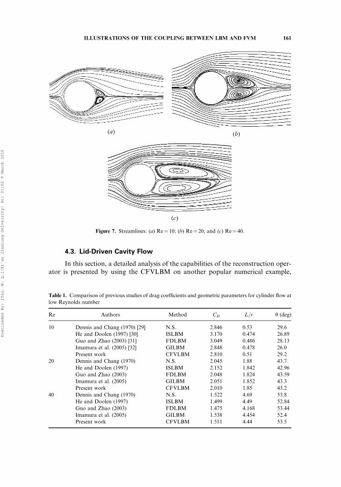
Here three small Reynolds numbers 10, 20, and 40 are chosen to validatethe proposed method. Figure 7 shows the streamlines when flow reaches its finalsteady state. A pair of vortices is observed behind the circular cylinder. For flowaround a circular cylinder there are three characteristic parameters: the length ofthe recirculation region L, the separation angle h, and the drag coefficient CD. CD

is defined as

CD ¼ 1

qu21r

ZS � n dl ð36Þ

where n is the normal direction of the cylinder wall and S is the stress tensor,

S ¼ �pI þ qtðruþ urÞ ð37Þ

The drag coefficient CD and the geometry parameters L and h are listed in Table 1.All of the parameters predicted by the CFVLBM agree well with the results ofprevious studies for each Re.

Figure 6. Flow around a circular cylinder.



4.3. Lid-Driven Cavity Flow

In this section, a detailed analysis of the capabilities of the reconstruction oper-ator is presented by using the CFVLBM on another popular numerical example,

Figure 7. Streamlines: (a) Re¼ 10; (b) Re¼ 20; and (c) Re¼ 40.

Table 1. Comparison of previous studies of drag coefficients and geometric parameters for cylinder flow at

low Reynolds number

Re Authors Method CD L=r h (deg)

10 Dennis and Chang (1970) [29] N.S. 2.846 0.53 29.6

He and Doolen (1997) [30] ISLBM 3.170 0.474 26.89

Guo and Zhao (2003) [31] FDLBM 3.049 0.486 28.13

Imamura et al. (2005) [32] GILBM 2.848 0.478 26.0

Present work CFVLBM 2.810 0.51 29.2

20 Dennis and Chang (1970) N.S. 2.045 1.88 43.7

He and Doolen (1997) ISLBM 2.152 1.842 42.96

Guo and Zhao (2003) FDLBM 2.048 1.824 43.59

Imamura et al. (2005) GILBM 2.051 1.852 43.3


40 Dennis and Chang (1970) N.S. 1.522 4.69 53.8

He and Doolen (1997) ISLBM 1.499 4.49 52.84

Guo and Zhao (2003) FDLBM 1.475 4.168 53.44

Imamura et al. (2005) GILBM 1.538 4.454 52.4




lid-driven cavity flow. The geometry and boundary conditions are shown in Figure 8.Three numerical simulations were carried out for Re¼ 100, 400, and 1000 on a gridof 400� 400. The characteristic length in Reynolds numbers is the height of thesquared cavity, H¼ 1. The boundaries of the cavity are still walls, except the upperboundary, for which a uniform tangential velocity is prescribed as uRe¼100¼3.33� 10�3, uRe¼400¼ 1.33� 10�3, uRe¼1000¼ 3.33� 10�2 for the three Reynoldsnumbers, respectively. Corresponding to each case, the Mach numbers are MaRe¼100¼5.77� 10�3, MaRe¼400¼ 2.31� 10�2, and MaRe¼1000¼ 5.77� 10�2.

Figure 9 shows the streamlines plots for the Reynolds number considered.These plots give a clear picture of the overall flow pattern and the effect of Reynoldsnumber on the structure of the recirculating eddies in the cavity. The smoothness ofthe streamline, especially around the hand-shaking region, further confirms the cor-rectness of the information transfer at the interface. In addition to the primary centervortex, a pair of counterrotating eddies of much smaller strength are developed inthe lower corners of the cavity. To quantify these results, the center locations ofthe primary vortices, bottom left vortices, and bottom right vortices are listed inTable 2. The results are in close agreement with the benchmark solution [33]. AsRe increases, the primary vortex center moves toward the right and increasinglybecomes circular.

Figures 10 and 11 show the contours of u velocity and v velocity. It is seen thatthese physical quantities are all smooth across the interface. The velocity profilesalong the vertical and horizontal centerlines of the cavity are shown in Figures 12and 13. It is seen that the maximum errors occur at the peak points. This is becausethe absolute values of velocity are larger at those points. Errors grow as Re increases.This may be partially caused by the weak compressibility of the LBM results. In theLBM zone, the density is not a constant inherently related to the LBM. However, theFVM model adopted here is incompressible. To illustrate this argument more

Figure 8. Lid-driven cavity flow.



clearly, Figure 14 shows the density contour lines of the predicted results. We cansee that the density is changing in the LBM zones. When the LBM and incompress-ible FVM are coupled, flow velocity should not be large, to decrease the com-pressibility influence by the LBM. All things considered, we conclude that theresults obtained by the CFVLBM are in good agreement with the benchmark workby Ghia et al. [33].

When the Navier-Stokes equations are used to solve the incompressible flow, itis crucial to maintain the mass conservation of the entire flow domain. This issue isespecially importance when the coupled method is used. The hand-shaking region is

Figure 9. Streamlines: (a) Re¼ 100; (b) Re¼ 400; and (c) Re¼ 1,000.

Table 2. Comparison of vortices location between present results and [33]

Re=vortices

Primary vortices

location (x, y)

Bottom left vortices

location (x, y)

Bottom right vortices

location (x, y)

Re¼ 100 Present (0.615, 0.738) (0.0325, 0.038) (0.936, 0.062)

Ref. (33) (0.6172, 0.7344) (0.0313, 0.0391) (0.9453, 0.0625)

Re¼ 400 Present (0.565, 0.609) (0.051, 0.046) (0.888, 0.124)

Ref. (33) (0.5547, 0.6055) (0.0508, 0.0469) (0.8906, 0.1250)

Re¼ 1,000 Present (0.537, 0.568) (0.083, 0.076) (0.861, 0.111)

Ref. (33) (0.5313, 0.5625) (0.0859, 0.0781) (0.8594, 0.1094)



best to examine the conservation of the mass flow rate. For this purpose, Figures 15and 16 are provide, where the mass fluxes at the interface (i.e., line A–B in Figure 8)at Re¼ 1,000 are shown. We can see that the mass fluxes from the LBM and FVMmatch very well.

The contours of vorticity distribution are now examined, and the results arepresented in Figure 17. The plots of vorticity with viscous effects are confined to thinshear layers near the wall. It can be observed that the vorticity contours predictedfrom the FVM and LBM are in agreement. However, there is some nonsmoothnessat the interface. We have tried several numerical methods (refining the grids, improv-ing convergence criteria), but this nonsmoothness could not be fully removed. Thusit is expected to be caused by the weak compressibility and unsteady nature of theLBM. This observation gives us a hint: to confirm good smoothness and consistencywhen coupling of numerical solutions at the interface is investigated, the quality ofthe vorticity contour plot is more sensitive to that of velocity. This is becausevorticity is the first derivative of velocity; its smoothness requirement is more strictthan that of velocity. The stream function is an integral of the velocity; hence itssmoothness is the easiest to obtain.

Finally, CPU time to obtain a steady-state solution of the lid-driven cavity flowis discussed. For the FVM, the steady-state solution can be obtained from a steadygoverning equation with an assumed initial field. This iterative process is in some

Figure 10. The u-velocity contour lines: (a) Re¼ 100; (b) Re¼ 400; and (c) Re¼ 1,000.



Figure 11. The v-velocity contour lines: (a) Re¼ 100; (b) Re¼ 400; and (c) Re¼ 1,000.

Figure 12. Comparison of u velocity along vertical line through geometric center.



Figure 14. Density contour lines: (a) Re¼ 100; (b) Re¼ 400; and (c) Re¼ 1,000.

Figure 13. Comparison of v velocity along horizontal line through geometric center.



sense similar to an unsteady solution process, with one outer iteration being equiva-lent to marching one time step forward. The LBM is an essentially unsteadyapproach in which the solution gradually evolves into steady state. In this articlethe iteration convergence criterion for reaching the steady state is defined byEq. (38) with err¼ 10�6.

Residual ¼PP

juði; j; tþ DtÞ � uði; j; tÞj þPP

jvði; j; tþ DtÞ � vði; j; tÞjPPðjuði; j; tÞj þ jvði; j; tÞjÞ � err

ð38Þ

Figure 15. The y component of the mass flux qv=(q0ulid) on the interface AB defined in Figure 8.

Figure 16. The x component of the mass flux qu=(q0ulid) on the interface AB.



The case of Re¼ 1,000 is selected to compare the residual history for fourmethods. The first method and the second method are the single FVM methodand the single LBM in the whole computation domain, respectively. The thirdmethod is denoted by CFVLBM(I), in which the interface information exchangeis executed after one outer iteration in the FVM region and one time step forwardin the LBM region. In the fourth method, denoted by CFVLBM(II), the interfaceinformation exchange is not executed until the interface mass residual defined byEq. (38) is almost equal to or even less than the mass residual of the entire subre-gion. Here, by one outer iteration in the FVM we mean that the coefficients of thediscretization equation are updated once. The inner iteration means the solutionprocess of the algebraic equation for the given set of coefficients in the discretiza-tion equations. For both the CFVLBM(I) and CFVLBM(II), the inner iteration isthe same.

When the flow reaches steady state, the flow fields obtained from the fourmethods are almost identical. However, the residual histories are quite different.Figure 18 shows the residual history of the four methods. It can be seen that theFVM method has the fastest convergence rate, the LBM shows the worst conver-gence speed, and the CFVLBM(I) and CFVLBM(II) are in between, with theCFVLBM(II) being much better than the CFVLBM(I).

Figure 17. Vorticity contour lines: (a) Re¼ 100; (b) Re¼ 400; and (c) Re¼ 1,000.



5. CONCLUSIONS

In this article, a coupling approach is used to combine the LBM and FVM forsimulating fluid flow problems. A reconstruction operator is adopted to lift themacroscopic velocity fields of the FVM to mesoscopic distribution functions ofthe LBM. Three numerical examples have validated the feasibility and reliabilityof the proposed reconstruction operator.

The stream function contours are the easiest to smooth. To confirm goodsmoothness and consistency of solutions coupling at the interface, the vorticity con-tours are suggested separately from the velocity distributions. The convergence tosteady-state flow is expected to be accelerated by the proposed CFVLBM(II).

Extension to higher Mach numbers and 3-D computations is now underway inthe authors’ group and will be reported later.

REFERENCES

1. E. Weinan, B. Engquist, X. Li, W. Ren, and E. Vanden-Eijnden, Heterogeneous Multi-scale Methods: A Review, Commun. Comput. Phys., vol. 44, pp. 367–450, 2007.

2. S. Succi, O. Filippova, G. Smith, and E. Kaxiras, Applying the Lattice BoltzmannEquation to Multiscale Fluid Problems, Comput. Sci. Eng., vol. 3, pp. 26–37, 2001.

3. Q. H. Zeng, A. B. Yu, and G. Q. Lu, Multiscale Modeling and Simulation of PolymerNanocomposites, Prog. Polymer. Sci., vol. 33, pp. 191–269, 2008.

4. W. Q. Tao, Numerical Heat Transfer, 2nd ed., pp. 1–26, Xi’an Jiaotong University Press,Xi’an, China, 2000.

5. F. F. Abraham, Dynamically Spanning the Length Scales from the Quantum to theContinuum, Int. J. Mod. Phys. C, vol. 11, pp. 1135–1148, 2000.

6. X. B. Nie, S. Y. Chen, W. N. E., and M. O. Robbins, A Continuum and MolecularDynamics Hybrid Method for Micro- and Nano-Fluid Flow, J. Fluid Mech., vol. 500,pp. 55–64, 2004.

Figure 18. Residual history for the lid-driven cavity flow for Re¼ 1,000.



7. A. Dupuis, E. M. Kotsalis, and P. Koumoutsakos, Coupling Lattice Boltzmann andMolecular Dynamics Models for Dense Fluids, Phys. Rev. E., vol. 75, pp. 046704, 2007.

8. J. S. Wu, X. Y. Lian, G. Cheng, P. R. Koomullil, and K. C. Tseng, Development andVerification of a Coupled DSMC–NS Scheme Using Unstructured Mesh, J. Comput.Phys., vol. 219, pp. 579–607, 2006.

9. P. L. Bhatnagar, E. P. Gross, and M. Krook, A Model for Collision Processes in Gases,Part I. Small Amplitude Processes in Charged and Neutral One-Component System, Phys.Rev., vol. 94, pp. 511–525, 1954.

10. X. He and L. S. Luo, A Priori Derivation of the Lattice Boltzmann Equation, Phys. Rev.E, vol. 55, pp. R6333-6, 1997.

11. X. He and L. S. Luo, Theory of the Lattice Boltzmann Equation: From BoltzmannEquation to Lattice Boltzmann Equation, Phys. Rev. E., vol. 56, pp. 6811–6817, 1997.

12. Y. H. Qian, D. d’Humieres, and P. Lallemand, Lattice BGK Models for Navier StokesEquation, Eur. Phys. Lett., vol. 15, pp. 603–607, 1991.

13. S. V. Patankar, A Calculation Procedure for Two-Dimensional Elliptic Situation, Numer.Heat Transfer, vol. 4, pp. 409–425, 1981.

14. J. P. van Doormaal and G. D. Raithby, Enhancement of the SIMPLE Method forPredicting Incompressible Fluid Flow, Numer. Heat Transfer, vol. 7, pp. 147–163, 1984.

15. R. I. Issa, Solution of the Implicit Discretized Fluid-Flow Equations by OperatorSplitting, J. Comput. Phys., vol. 62, pp. 40–65, 1986.

16. R. H. Yen and C. H. Liu, Enhancement of the SIMPLE Algorithm by an AdditionalExplicit Correction Step, Numer. Heat Transfer B, vol. 24, pp. 127–141, 1993.

17. B. Yu, H. Ozoe, and W. Q. Tao, A Modified Pressure-Correction Scheme for theSIMPLER Method, MSIMPLER, Numer. Heat Transfer B, vol. 39, pp. 435–449, 2001.

18. W. Q. Tao, Z. G. Qu, and Y. L. He, A Novel Segregated Algorithm for IncompressibleFluid Flow and Heat Transfer Problems—Clear (Coupled and Linked EquationsAlgorithm Revised) Part I: Mathematical Formulation and Solution Procedure, Numer.Heat Transfer B, vol. 45, pp. 1–17, 2004.

19. W. Q. Tao, Z. G. Qu, and Y. L. He, A Novel Segregated Algorithm for IncompressibleFluid Flow and Heat Transfer Problems—Clear (Coupled and Linked Equations Algor-ithm Revised) Part II: Application Examples, Numer. Heat Transfer B, vol. 45, pp. 19–48,2004.

20. D. L. Sun, Z. G. Qu, Y. L. He, and W. Q. Tao, An Efficient Segregated Algorithm forIncompressible Fluid Flow and Heat Transfer Problems—IDEAL (Inner Doubly IterativeEfficient Algorithm for Linked Equations) Part I: Mathematical Formulation andSolution Procedure, Numer. Heat Transfer B, vol. 53, pp. 1–17, 2008.

21. D. L. Sun, Z. G. Qu, Y. L. He, and W. Q. Tao, An Efficient Segregated Algorithm forIncompressible Fluid Flow and Heat Transfer Problems—IDEAL (Inner Doubly IterativeEfficient Algorithm for Linked Equations) Part II: Application Examples, Numer. HeatTransfer B, vol. 53, pp. 18–38, 2008.

22. Z. Y. Li and W. Q. Tao, A New Stability-Guaranteed Second-Order Difference Scheme,Numer. Heat Transfer B, vol. 42, pp. 349–365, 2002.

23. W. Q. Tao and Y. L. He, Recent Advances in Multiscale Simulations of Heat Transferand Fluid Flow Problems, Prog. Comput. Fluid Dynam., vol. 9, pp. 150–157, 2009.

24. H. Xu, H. B. Luan, and W. Q. Tao, A Reconstruction Operator for the InterfaceCoupling between LBM and Macro-numerical Methods of Finite-Family, J. Xi’anJiaotong Univ., vol. 43, no. 11, pp. 6–10, 2009 (in Chinese).

25. U. Frisch, D. d’Humieres, B. Hasslacher, P. Lallemand, Y. Pomeau, and J. P. Rivet,Lattice Gas Hydrodynamics in Two and Three Dimensions, Complex Syst., vol. 1,pp. 679–707, 1987.



26. D. A. Wolf-Gladrow, Lattice Gas Cellular Automata and Lattice Boltzmann Models: AnIntroduction, pp. 175–190, Springer-Verlag, Berlin, 2000.

27. W. Q. Tao, Recent Advances in Computational Heat Transfer, pp. 337–352, Science Press,Beijing, 2005.

28. B. F. Armaly, F. Durst, J. C. F. Pereira, and B. Schonung, Experimental and TheoreticalInvestigation of Backward-Facing Step Flow, J. Fluid Mech., vol. 127, pp. 473–496, 1983.

29. S. Dennis and G. Chang, Numerical Solutions for Steady Flow past a Circular Cylinder atReynolds Number up to 100, J. Fluid Mech., vol. 42, pp. 471–489, 1970.

30. X. He and G. Doolen, Lattice Boltzmann Method on Curvilinear System: Flow around aCircular Cylinder, J. Comput. Phys., vol. 134, pp. 306–315, 1997.

31. Z. Guo and T. Zhao, Explicit Finite-Difference Lattice Boltzmann Method for Curvi-linear Coordinates, Phys. Rev. E, vol. 67, pp. 066709-1–066709-12, 2003.

32. T. Imamura, K. Suzuki, T. Nakamura, and M. Yoshida, Acceleration of Steady StateLattice Boltzmann Simulation on Non-uniform Mesh Using Local Time Step Method,J. Comput. Phys., vol. 202, pp. 645–663, 2005.

33. U. Ghia, K. N. Ghia, and C. T. Shin, High-Re Solutions for Incompressible FlowUsing the Navier-Stokes Equations and a Multigrid Method, J. Comput. Phys., vol. 48,pp. 387–411, 1982.



numerical heat transfer, part b: fundamentals numerical ...nht.xjtu.edu.cn/paper/en/2010208.pdf ·...

Documents