numerical integration methods for ballistic rocket ... · numerical integration methods for...
TRANSCRIPT

ECOM-5134
JUNE 1967
AD
■
00
to
NUMERICAL INTEGRATION METHODS FOR BALLISTIC ROCKET TRAJECTORY SIMULATION
PROGRAMS
By
Randall K. Walters
D D C \pr^r~ nr r "~»<
Or ^< SEP 12 1967
ATMOSPHERIC SCIENCES LABORATORY WHITE SANDS MISSILE RANGE, NEW MEXICO
Distribution of this report is unlimited.
ECOM UNITED STATES ARMY ELECTRONS COMMAND
ifi

NUMERICAL INTEGRATION METHOPS FOR
BALLISTIC ROCKET TRAJECTORY SIMULATION PROGRAMS
By
RANDALL K. WALTERS
ECOM - 5134 June 1967
DA TASK IV014501BS3A-10
ATMOSPHERIC SCIENCES LABORATORY WHITE SANDS MISSILE RANHE, NEW MEXICO
Distribution of this report is unlimited.

I r *
ABSTRACT
Numerical integration methods for solution of the system of differential equations found in ballistic rocket trajectory programs are discussed.
The general discussion entails the explicit formulas of Runge- Kutta and predictor-corrector methods and their errors, and a brief description of other methods that could be employed.
111

CONTENTS
Page
ABSTRACT — « — iii
INTROLXTION 1
RUNGE-KUTTA METHODS
Formulas ■ —- — 1
Error 5
Analysis 7
MULTISTEP METHODS
Standard Predictor-Corrector Methods 8
The Generalized Predictor-Corrector 12
Analysis of Predictor-Corrector Methods 16
OTHER GENERAL METHODS
Block Method - - 17
Hybrid Method —— 18
SUMMARY 18
REFERENCES 20
APPENDIX A - 22

INTRODUCTION
In a ballistic rocket trajectory simulation program the system of differential equations used to describe the ballistic model is a highly complex system. In particular the six-degree of freedom model used by the Atmospheric Sciences Office at White Sands Missile Range, consists of a system of twenty-one 2nd order ordinary differen- tial equations which are to be solved for the ballistic rocket's com- ponents of acceleration, velocity, and position at discrete time in- tervals. The most feasible method for solving the system is to pro- gram it for a computer and solve by some numerical integration orocedure.
This report will present several numerical integration schemes which are currently being used or are feasible for use in a ballistic rocket simulation program.*
RUNGE-KUTTA METHODS
Formulas
Consider the system of first order differential equations
dyi y[ ■ ^ - fA(x, yjtx), y2(x), ..., yN(x)) (1)
satisfying the initial conditions
y.(x ) * y. . (2) 7iv o' 7io '
We desire the values of y.(x ♦ h), i « 1, 2, ..., N, where h is the
increment in the independent variable.
*This report was presented to the Second Annual Conference on Pure and Applied Mathematics held at New Mexico Institute of Mining and Technology, Socorro New Mexico, Feb. 24-25, 1967.

The Runge-Kutta method is an algorithm designed to approximate the Taylor series solution
y.(x ♦ h) » y. ♦ h y.(1}(x ) ♦ ~ y.(2)(x ) 7i^ o ' 720 7i * o 2 7i * oJ
♦F^cy*- (3)
fk) of (1), where y. '(x ) denotes the kth derivative and i = 1, 2,
..., N. However, in deriving the defining equations of the algorithm, the use of the appropriate assumptions makes it unnecessary to eval- uate and define the derivatives of higher order.
The general equations defining a fourth order Runge-Kutta method are given by
Ki *hf <v V K2 = hf(xQ * ah, yQ ♦ 0Kj)
K3 = hf(xQ ♦ c^h, yQ ♦ 0^ ♦ v^)
K4 * hf (xQ ♦ a2h, yQ ♦ 0^ * yfo + 6 fa)
K = 7(X0 * h) - yQ = n1K1 ♦ »fa ♦ ufa * y^
(4)
where the bar denotes an approximate value.
The thirteen parameters involved are found by expanding K" about the point (x , y ) so as to agree with the Taylor series expansion
(3) up to and including terms of order h ; thus, the fourth order method. Initially, the solution will result in eight equations in thirteen unknowns. However, under the appropriate afsumptions, the system will resolve into a system of eight equations in nine rnknowns, hence a one parameter family.

One solution is the classical formulas of Runge, given by,
K, - hf (x . v ) O' '0'
K2 = hf (xo * £, yo ♦ jt)
K3 " hf <Xo 4V r> (5)
K4 = hf(xo ♦ h, yo t K3)
K = ^ (Kj * 2K2 * 2K3 + K4)
One will notice that when y' = f(x), Runge 's formulas reduce to Simp- son's rule:
x *h . K = / ° f(x)dx = 2. [f(xo) ♦ 4f (xrt + y) * f(xn ♦ h>]
0 \> T 2J (6)
Another solution to the one parameter family is the classical formulas of Kutta given by
K, * hfK> YJ o' 'o'
K2 « hf (xo ♦ £, yQ * jij
2h *1 *2 (7)
K. » hf (x„ ♦ h, y ♦ K. - K- ♦ K.)
K « j (Kj + 3K2 ♦ 3K3 ♦ K4)
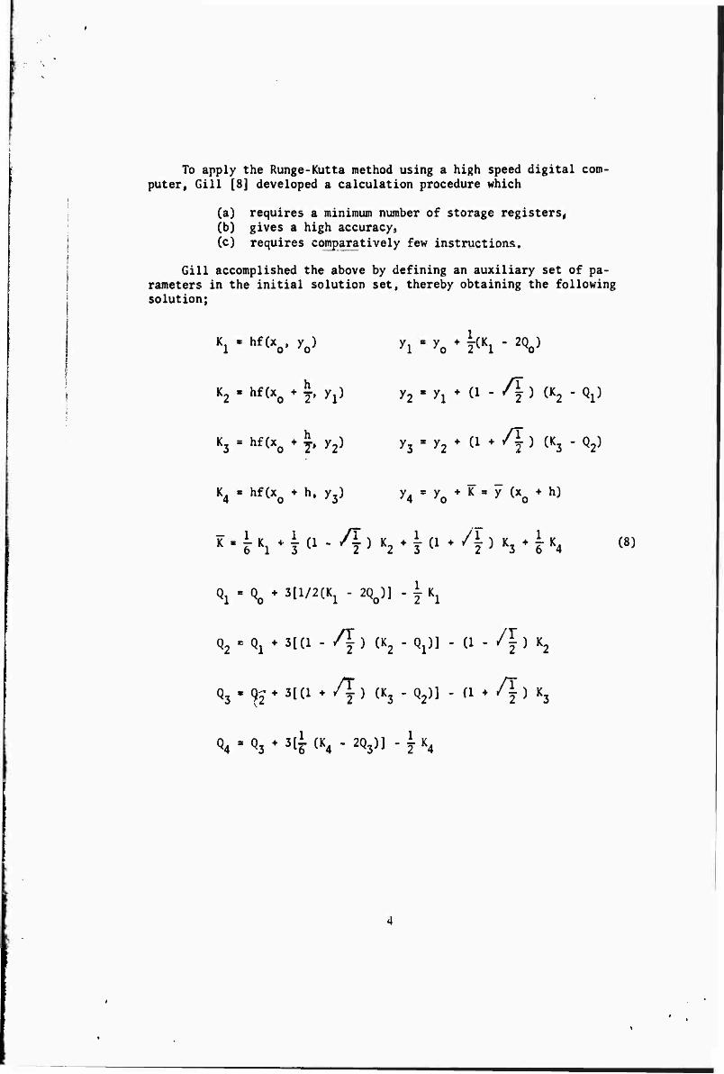
To apply the Runge-Kutta method using a high speed digital com- puter. Gill [8] developed a calculation procedure which
(a) requires a minimum number of storage registers, (b) gives a high accuracy, (c) requires comparatively few instructions.
Gill accomplished the above by defining an auxiliary set of pa- rameters in the initial solution set, thereby obtaining the following solution;
Ki -hf <v *0>
K2 . hf(x0 ♦ £, Xl)
1
y2 • yx + (i - /j) (K2 - Qj)
h • hfC*0 ♦ j. y2) y. - y, ♦ (1 ♦ /I ) (K. - Q,) '3 '2 j x2,
K4 - hf (xo ♦ h, y3) v*' y0 * K " y (xo * h)
K.^Ki+|(l.4)K2+I(l + /i)K3 + lK4 (8)
^•%* 3[1/2(K1 - 2Qo)] - i Kx
Q2 ■ Qj ♦ 3[(1 - /I ) (K2 - Qj)] - (1 - /I ) K2
Q3 • Qj ♦ 3[(1 ♦ /I ) (K3 - Q2)] - (1 ♦ /i ) K3
Q4 - Q3 ♦ 3[I (K4 - 2Q3)] - \ K4

where the Q. are the auxiliary parameters. Initially 0 is zeroj
to compensate for the round-off error in y.. Q,, is used as the Q in
the next step. For a complete discussion of the algorithm and a flow chart, refer to [16].
Error
To obtain^a general expression for truncation error per step, the functions K = y(x ♦ h) - v and K * y(x +h) - y are expanded
through terms of h , thus giving the per-step truncation error as
E s K -K* mo [-r - 3(S2T - ST2 * f2y
+ 3f P ♦ 2f ST - 4f3 T) ♦ 2f T3] ♦ ... (9) yy y y y J J
where TK = DKf, SK = DKfy,P = (Df)2.
Lotkin [12] determined a bound for L which is given by
|E| < jg ML4h5 (10)
where in R*, a region containing (x , y ),
|f(x. y) | ! M,
and
io r i < L
3X1 3yJ MJ '
where the positive constants M and L, are independent of (x, y), for i ♦ j ? 4.
(11)

A numerical integration method is called stable if at the nth step, the total error, which is both truncation and round-off error, is at a minimum*thereby forcing the approximate solution to tend to the true solution.
Hence, as for the stability of the Runge-kutta methods, Carr [3) proved a theorem, of which the essential parts are stated below:
Let f be continuous, negative and bounded from above and
below in some region R of the (x, y) plane, i.e., M2 > M. > 0, fy
c(~M2, - M ); further, let E be the absolute value of the maximum
error introduced at each step, and D* be a region in which the so- lution of the difference equation tends to the y-boundary of D no closer than Qh ♦ |e.j, where
Qimax |f(x, y)| i max l\A9\A$ |KJ] x,yeD Z 2 3
(12)
and e. is the error at the ith step. Then, the Kutta fourth order
method has a bound on the total error in the ith step, where this bound is given by
fei' - hM, (13)
in some region D*, and where the step-size, h, is given by
M 4M.3
h < min (—y , —3-). M2 M2
(14)
If, f I 0 (the unstable case), but bounded throughout Ü, 0 5 f 5 M, then the propagated error, X. . in U* at the
(i ♦ 1) st step is given by
Ki\ - i£ite hM (15)

and
ihM
and E and h are as given before.
Statements (13), (14), (15) relate the step-size and the prop- agated error. Thus, an h can be found that will make the propagated error less than a certain bound, if this bound is the known bound on the partial derivative. Algorithms for finding such step«sizes can be found in Carr [3].
Although various bounds on the truncation error are known, such as the one given above, their usage in a computer program is usually not feasible. Thus, some practical scheme for estimation of this error must be devised.
One such scheme was devised by Richardson [5]. This scheme is based on numerically integrating with step-sizes of h and h. and
comparing the results using these step-sizes. A variation of this which we use is the following:
Let Y be the true value of y at x +h, y^ * the value ob- (2)
tained at x +h using h. » h, yv the value obtained at x +h (16)
using h9 ■ h . Then for small h,
7 (2) " y
The scheme in (16) can be used to check the validity of the answer for the purpose of halving and doubling the step-size h.
Analysis
By virtue of the Runge-Kutta methods requiring only information from one previous step, the method has desirable stability charac- teristics and ease of halving or doubling the step-size h.
It has been shown, however, by Blum [2] and Fyfe [6], that through proper redefinition of the solution set of parameters, most other versions of the fourth order Runge-Kutta method can avail themselves of the reduced storage of the Gill algorithm.

If the first derivative of the functions are very involved, then several evaluations of these first derivatives may be somewhat time consuming and thus cause the method to be uneconomical at times. Another distinct shortcoming of the method is that of the error. Neither truncation error, nor its estimate, is obtained in the cal- culation procedure, thus necessitating the approximate comparisons described previously.
Finally, the Runge-Kutta methods can be used as a starting pro- cedure for other methods, such as multistep methods.
j > MULTISTEP METHODS
i Standard Predictor-Corrector Methods
A multistep method is a method in which the calculation of the y.*s at the (M+l) st step depends on knowledge of the yi's and the
f^s at the Mth, (M-l) st, (M-2)nd, etc. steps. A method is called
alim-step method if only m-steps of previous information are required. In the following discussion only four-step methods will be considered since methods with fewer back values can be extracted from the dis- cussion below.
The multistep method with which we are concerned here is known as the predictor-corrector method. This method requires a formula for finding a first estimate of each y. (hence, the predictor); and
then evaluating each function f. we substitute this into a formula
which will adjust the value obtained from the predictor, hence the corrector. By a standard method we mean one in which the same step- size is used in all the equations in integrating for each y..
First of all, rewrite the system of differential equations in (1) as
y.' » f^x, yr y2, ..., yN) (17)
with the initial conditions
yi(xo} * yi(0) (18)

We desire the values y(x +h), i « 1, 2, ... N where h is again the
increment in the independent variable.
Next let us clarify some notation which we will be using.
y.(M) - y. (xo *Mh)
P
i « 1, 2, ..., N
(M*l) » y.(xQ ♦(M+l)h) i - 1, 2, ..., N
•(M) « y.'(xo+Mh) * f\(xo*Mh, y.(M), y2(M), .... yN(M))
'(M+l) » 7.»(xo*(M+l)h) « f.(xo*(M*l)h, ^(M+l), ..., PN(M*1)
(19)
(M+l) = yi(xo*(M+l)h) I ■ 1, 2, .».. N
By using (17), the defining equations for the standard predictor- corrector algorithm are given by
P^l) « aiy.(M) ♦ b^M-l) ♦ Ciy.(M-2)
♦d^OMMiIe^OO ♦ f^.^M-l) (20)
* «xXi'01-2) ♦ Kiyi«(M-3)], i * 1,2, ..., N
C.(M*1) » a2y.(M) ♦ b2y.(M-l) ♦ C2y.(M-2)
* h[d2y.»(M+l) ♦ e2y.»(M) ♦ f^'QM) (21)
* g2yi,(M-2)], i «1, 2, ..., N
where (20) is the predictor, (21) the corrector, and the coefficients are to be determined.

Using the standard technique of [10] for solution of the con- stant coefficients, the solution set is:
a. ■ 9 - d. - 3e. ♦ 3K. a2 « 9 - 15d2 - 3e2
bx » 9 - 9d. ♦ 24KX b2 « 9 - 24d2
cx - - 17 ♦ 9dx ♦ 3e2 - 27^ c0 « - 17 ♦ 39d~ ♦ 3e.
di-«4 d2"d2 (22)
el'el e2se2
f: « - 18 + ödj + 4e2 - 17KX; f2 » - 18 ♦ 39d2 + 4e
gj * - 6 + Mj ♦ ex - 14KX; g2 = - 6 + 14d2 + e2
Kl-Kl
Since the coefficients in (22) are in terms of the parameters d., e., Kj, d2, e2, the constants can be determined so as to give
desirable stability characteristics.
The truncation error in the predictor-corrector equations is given by
EP * TO <9 + 3di - ei - 10Ki> h$ yis)
Ec . ^ (9 - 24d2 - • ) h5 y&
(23)
where fc and E are the predictor and the corrector truncation error. p c -*
respectively. However, the predictor and the corrector were chosen independently of fourth order. Consequently, from Henrici [11 , p 261],the truncation error of the algorithm is given by h alone.
10

1
But, yl ' may not be available; thus, some means for reflecting the truncation error must be made available.
The standard technique for adjusting P.(M+1) with respect to
the local truncation error is to add
E(M+1) * g P£ (P.(M) - C.(M)) c p
(24)
to P.(M+1), to improve its value. Notice the fact that E(M+1) will (S)
not involve y .
Similarly, the common method of keeping track of the total trun- cation error is to use
ET(M+1) = g £_ (p.(M*l) - C. (M+l)) c p
(25)
as an estimate of this error at the (M+l) st step, and from (25) criteria for halving and doubling the step-size h can be generated.
According to Crane and Klopfenstein [4], the values for the con- stants in (22) which yield a stability situation not unlike that of Runge-Kutta methods are given by
c, «
25 1.54765200 a2 * 1.0000
S -1.86750300 b2 * 0.
s 2.01720400 c2 * 0.
« -0.697353000 d2 « 0.375000000
a 2.00224700 62 « 0.791666667
-2.03169000 f2 *-0.208333333
ss 1.81860900 *2 = 0.041666666
. * -0.714320000
e, *
(26)
11

where the trailing zeros are used to make the method as "numerically" fourth order as possible. The coefficients in the corrector equation determine the standard Adams - Mculton corrector.
The Generalized Predictor-Corrector
By using the standard predictor-corrector formulas as discussed in the preceding section, one inherent shortcoming arises; that of using the same fixed step-size h in integration of the various y.'s.
In many physical situations, and particularly in the mathematical model representing the trajectory of a ballistic rocket, the system of differential equations that arise may have some solutions vary- ing much more rapidly than others with respect to the independent variable. Since the step-size must be chosen to give the desired accuracy in the most rapidly varying solution, by using the standard predictor-corrector, computer time may be wasted in integrating the slower varying solutions thru use of the short step-size h. Thus, the need arises for a generalized predictor-corrector algorithm in which the step-sizes may be different in each equation. To this end, we wish to use an increment h. in the ith equation where h. . ■ m.h.,
l n l-l l i* i = 2, 3, ..., N and m. is a positive integer.
One would like to progress to the point x + h. by means of one
predictor-corrector step in the first equation, m- steps in the sec-
ond equation, nu m- steps in the third equation , .., nu m_ ... m..
steps in the Nth equation. That is, we don't wish to calculate each f. « y! at any points between x ♦ Mh. and x ♦ (M+l)h., i » 1, 2,
..., N.
Suppose for the moment we have a method of calculating
hi y^r.) for r.h. * jjy j » 1, 2, ..., jj±-, i « 1, 2, ..., N-l. N
Let this method be denoted by (*). We call (*) the generalized pre- dictor as will be borne out in the following discussion.
12
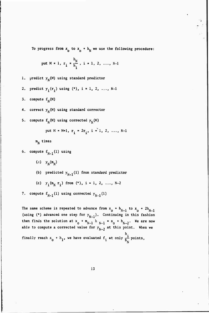
To progress from x to x ♦ h we use the following procedure:
hN put M « 1, r. « jj- , i - 1, 2, ..., N-l
i
1. predict yN(M) using standard predictor
2. predict yi(ri) using (*), i * 1, 2, ..., N-l
3. compute fN(M)
4. correct yN(M) using standard corrector
5. compute fN(M) using corrected yN(M)
put M = IM, r. = 2r.t i »Nl, 2, ..., N-l
nu. times N
6. compute *"N i(l) using
(A) yN(mN)
(b) predicted yN i(l) from standard predictor
(c) y.(mN r.) from (*), i « 1, 2, ..., N-2
7. compute fN .(1) using corrected yN .(1)
The same scheme is repeated to advance from x ♦ h., , to x ♦ 2hk, , r o N-l o N-l (using (*) advanced one step for yN i). Continuing in this fashion
then finds the solution at x ♦ BL, , h x. , ■ x ♦ h . we are now o N-l N-l o N-2
able to compute a corrected value for yN 2 at this point. When we
h. finally reach x ♦ h., we have evaluated f. at only —points,
13

i * 1, 2, ..., N. For a simple example illustrating the above pro- cedure see Appendix A.
Now it only remains to determine the generalized predictor (*) for calculating the predicted value of y.(y), where y is the inter-
mediate value of M, 0 < y < 1. To do this, write (20), the standard predictor, in the form.
P^Y) = ax(Y) y.(M) ♦ ^(Y) yi(M-l) ♦ CI(Y) y.(M-2)
♦ ^(Y) y.(M-3) ♦ h.fe^Y) y!(M) ♦ ^(Y) y!(M-l) (27)
♦ g^Y) y?(M-2) ♦ KXCY) y!(M-3)]
where the constant coefficients are to be determined and the follow- ing notation is used:
Pt(Y) * yi(xQ ♦ Yht)
yt(M) = yi(xQ ♦ Mh.)
i - 1, 2, ..., N
i = 1, 2, ..., N (28)
y!(M) = y!(XQ + Mh.) i » 1, 2, ..., N
to be By the same technique employed before, the solution set is found
ax(Y)
bj(Y) =
c^Y)
- dx(Y) -3ei(Y) ♦ 3KX(Y) ♦ 1/4 (Y4 + 6Y3 ♦ 13Y3 * 12 * r)
-9dx(Y) ♦ 24KX(Y) + (Y4 * 4Y3 * 4Y
2)
9dx(Y) * 3ei(Y) - 27KX(Y) - 1/4 (5Y4 * 22Y
3 + 29Y2 * 12Y)
dx(Y) = dx(Y) (29)
14

e1(Y) - ej(Y)
F^Y) = -M^y) * 4ej(Y) - 17K M - {y4 * 5Y3 ♦ 8Y2 ♦ 4Y)
g^Y) * MX(Y) ♦ ex(Y) - HKjM - 1/2 (y4 + 4Y3 ♦ SY2 ♦ 2Y)
The corresponding truncation error in the generalized predictor is given by:
E = 12dx(Y) - 4ej(Y) + 40^(7)
5 4 3 2 h5y(S) ♦ (y* ♦ 6Y4 * liyA * 12Y^ + 4Y) J£ (30)
As before, the standard technique for improving P.(Y) is to add
BW - ,-a,. (p.. c.) (31)
to P.(Y), where E. is E at y = 1, E is from (23), P. is the pre-
dieted value of the previous step and C. is the corrected value of
the previous step. t
Similarly, the truncation error in standard corrector is reflected in
ET (M+l) . -J-L- (, 0M) - CN(M+1)) c c p (32)
where E and E are the respective truncation errors in the standard
predictor-corrector. By calculating ET (M+l), the validity of the c
answer found by using the standard predictor-corrector may be checked.
15

However, the task of accounting for the truncation error in the steps using the generalized predictor is somewhat different. Since only predicted values from the generalized predictor are available at intermediate steps, the truncation error in the generalized pre- dictor is reflected in
*T M * F TT #4 * *0> i " l> 2> •"• N-1 (33) ]P fcc " fil -1 x
where E. is E at y * 1, and P. and C. are the predicted and corrected
values, respectively, obtained at the current step. This value must be used throughout the current stage.
Analysis of Predictor-Corrector Methods
One basic shortcoming in all predictor-corrector methods is that they require some other procedure to obtain enough values so as the method can be started. In the case of the generalized predictor- corrector, some procedure must be used to generate the first 3(m.)
steps in the ith equation. One method of starting the proceudre is the Runge-Kutta method.
One distinct disadvantage of the predictor-corrector methods is the difficulty in halving the step-size h. By utilizing the gen- eralized predictor-corrector some of these difficulties can be sur- mounted. Still, sometimes halving one of the increments is required, necessitating interpolation or even restarting the current step.
Stability of the predictor-corrector algorithms was not discus- sed here due to the lengths that one is required to go to an ade- quate discussion. Suffice it to say, the system of differential equations to be solved must be carefully examined to determine what odd characteristics exist and then the proper type of predictor-cor- rector algorithm chosen to give the desired stability and accuracy. For a further discussion see [10].
Predictor-corrector methods in general, are much faster than the Runge-Kutta methods and in particular, use of the generalized predic- tor will reduce the function evaluations per step and hence further reduce computer time used.
16

V
%
■ß \\
A
Block methods can also be applied to predictor-corrector schemes to improve their accuracy and efficiency. For a more complete dis- cussion of block methods, see [17],
Hybrid Method
Hybrid methods differ from those previously described in that in addition to using previous information from the M, (M-l)st, (M-2)nd, etc. steps, an outside method is used to calculate information at some (M-y)th step, 0 < y < 1, and this information is also incorporated into the multistep procedure.
In certain cases the added information tends to stabilize the formula in which it is used and makes halving the step-size an easier task.
However, as pointed out in Gear [7], situations arise in which the use of the added information introduces much more error into the solution of the system than is desirable. For a more thorough dis- cussion of hybrid methods, see [7] and [9].
SUMMARY
The Runge-Kutta algorithm can be used for the solution of most systems of differential equations. Since only information from one previous step is required, the Runge-Kutta methods have favorable stability characteristics and the process of altering the step-size is an easy task. Consequently, Runge-Kutta methods are frequently used as a starting procedure for other methods such as multistep methods. However, the number of function evaluations per step required by the Runge-Kutta methods requires'utilizing more computer time than multi- step methods and since no measure of the truncation error is avail- able during the calculation procedure, approximate or comparison methods are required in the program to reflect this error.
Multistep methods require fewer function evaluations per step and hence use less computer time. The truncation error can be meas- ured effectively during the calculation procedure, thereby exhibit- ing the error more correctly than do Runge-Kutta methods. The sta- bility of the predictor-corrector method should be investigated thor- oughly to determine what regions of integration are required for
18

efficient use of these methods. Although a smaller step-size is gen- erally required for predictor-corrector methodsras compared to the Runge- Kutta method, the use of the generalized predictor-con ector method may alleviate many problems found in multistep methods and may use the least computer time of all the methods described.
The fairly attractive methods briefly described in the final section point out other methods^ that stem from the Runge-Kutta and the multistep methods, that may be investigated for use in a ballistic rocket trajectory program due to their composite of the desirable characteristics of the Runge-Kuttr and multistep methods.
At the present time the Atmospheric Sciences Office at White Sands Missile Range is programming the generalized predictor-correc- tor algorithm for use in the six-degree of freedom ballistic rocket model. It is felt that this algorithm can best accomplish the desired task with a minimum of computer time and with accuracy comparable to that of Runge-Kutta methods used currently.
10

REFERENCES
1. Berezin, I. S., and N. D. Zhidkov, Corngutin^,Methods, Vol. 2, Trans, by 0. M. Blunn, Pergamon Press, Reading", Mass., 1965.
2. Blum, E. K., MA Modification of the Runge-Kutta Fourth Order Method/' Math, of Comp., Vol. 16, 1962, pp. 176-187.
3. Carr, J. W., "Error Bounds for the Runge-Kutta Singlestep Integra- tion Process," J. Assoc. Comp. Mach., Vol. 5, 1958, p. 39.
4. Crane, R. L., and R. W. Klopfenstein, "A Predictor-Corrector Al- gorithm with an Increased Range of Absolute Stabilit//' J. Assoc. Comp. Mach.. Vol. 12, 1965, pp. 227-241.
5. Forrington, C.V.D., "Extensions of the Predictor-Corrector Method for Solution of Ordinary Differential Equations." Comp. J.. Vol. 4, 1961, pp. 80-84.
r
6. Fyfe, David J., "Economical Evaluation of Runge-Kutta Formulae," Math, of Comp.. Vol. 20, 1966, pp. 392-398.
7. Gear, C. W., "Hybrid Methods for Initial Value Problems in Ordinary Differential Equations,' J. SIAM Numerical Analysis^ Ser. B. Vol. 2, 1965, pp. 69-8oT~ —
8. Gill, S., "A Process for the Step-by-Step Integration of Differen- tial Equations in an Automatic Digital Computing Machine," Proc. Cambridge Phi los. Soc, Vol. 47, 1951, pp. 96-108.
C 9. Gragg, W. B., and K. J. Stetter, "Generalized Multistep Predic-
tor-corrector Methods," J. Assoc. Comp. Mach. Vol. II, 1964, pp. 188-209.
10. Hamming, R. W., Numerical Methods for Scientists and Engineers, McGraw-Hill Book Co., New York, 1962.
11. Henrici, Peter, Discrete Variable Methods in Ordinary Differential Equations, John-Wiley and Sons, Inc., New York, 1962.
12. Lotkin, Max., "On the Accuracy of Runge-Kutta's Methods," MTAC, 1951, pp. 96-108.
13. Noble, B., Numerical Methods: Differences, Integration and Dif- ferential Equations, John-Wiley and Sons, Inc., New York, 1964,
20

14. Nordsieck, Arnold, "On Numerical Integration of Ordinary Differen- tial Equations." Math. Comp.. Vol. 16, 1962, pp. 22-49.
15. Richardson, L. E., and J. A. Gaunt, "The Deferred Approach to the Limit." Trans, ftpv. Soc. London. Vol, 226A, 1927, p. 300.
16. Romanelli, Michael J., "Runge-Kutta Methods for the Solution of Ordinary Differential Equations," Chapt. 9 of Mathematical Methods for Digital Computers, John-Wiley and Sons, Inc., New York, 1965"
17. Rosser, J. Barkley, "A Runge-Kutta for all F isons," MRC Technical Summary Report No. 698, September 1966
18. Walters, Randall K., "A Generalized Predictor-Corrector Method for the Solution of Ordinary Differential Equations," to be published in Transactions of the Twelfth Conference of Army Mathematicians.
21

APPENDIX A
An Example Using the Generalized Predictor-Corrector Method
Suppose we have the following system of first order differential equations
V ■ fi <x' yx> y2' y3}
y2« * f2 (x, yv yv y£ (34)
yZ * f3 (x' yV y2> y3}
where y2 varies three times as rapidly as y. with respect to x, and
y- varies twice as rapidly as y2 with respect to x. We would like
to find the solution of (34) at the point x ♦ h.. Therefore, let
h. = 3h2 and h2 = 2h_ where h. is the increment in the ith equation.
This means that üU = 3 and m. = 2. The following figure will illus-
trate this situation.
xrt K + hi o o 1
h'>
y2;
y-if
x x ♦ h~ x ♦ 2h~ x + 3hn o o 2 o 2 o 2
x x ♦ h, x + 6h> o o 3 o 3
In finding the solution of (34) at x ♦ h. we will calculate f. at x + h. only, L at x + h- and x ♦ 2h~ only and f. at x + Kh7, O 1 ' * 2 o 2 O 2 J 3 0 3 K = 1, 2, ..., 6, and use the generalized predictor for finding the y's between these points.
22

The detailed procedure is the following:
h3 1. put r. * r— , i » 1, 2 i
2. a. predict y (1) using the standard predictor
b. predict yx (r^ = yx (1/6) using (*)
c. predict y2 (r2) * y2 (1/2) using (*)
3. compute f_ (1), correct y- (1) using the standard corrector
and then compute a final value of f. (1)
4. put r. = 2r. = m- r., i * 1, 2 1 i ox
5. a. predict y- (2) * y_ (m.) using the standard predictor
b. predict yJ (rj) = yx (2/6) using (*)
c. predict y2 (rj = y2 (1) using the standard predictor
6. compute f- (2), correct y- (2) using the standard corrector,
and then compute a final value of f_ (2)
7. compute f2 (1) using 5, correct y2 (1) using the standard
corrector, and then compute a final value of f2 (1)
In the second equation we are now at the point x + h». We now ad-
vance (*) one step when using it in the second equation and it will be understood that when we say "predict y2 (r2), 0<r2<l, using (*)M
h'e mean we are predicting the value of y~ between x ♦ h0 and x * 2h . r ° '2 o 2 o 2 h3 - ■' /
8. put rx = ZT1 = (m3 ♦ 1) ty r2 = ^-
9. a. predict y,. (3) using the standard predictor
b. predict yx (r^ = yx (3/6) using (*)
c. predict y2 (r2) = y2 (1/2) using (*)
23

10. compute f- (3), correct y- (3) using the standard corrector
and then compute a final value of f. (3)
11. put r. * 4rx = 2m3 r., r2 » 2r2 « m7 r2
12. a. predict y. (4) « y_ (2m.) using the standard predictor
b. predict yx (r^ = yx (4/6) using (*)
c. predict y2 (r2) « y2 (1) using the standard predictor
13. compute f, (4), correct y- (4) using the standard corrector,
and then compute a final value of f_ (4)
14. compute f (1) using 12, correct y2 (1) using the standard
corrector and then compute a final value of f~ (1)
Again we advance (*) one step when using it in the second equation. We will now compute y2 (r2), o<r2<l between x ♦ 2h2 and x ♦ 3h2.
h 15. put rx » Srj « (2m3 + 1) r1> r2 » ^-
m
16. a. predict y- (5) using the standard predictor
b. predict yx (r^ = yx (5/6) using (*)
c. predict y2 (r2) * y^ (1/2) using (*)
17. compute f- (5), correct y» (5) using the standard corrector,
and then compute a final value of f- (5)
18. put r. » 6r, * m- m2 r., r2 = 2r2 = m- r2
19. a. predict y- (6) = y- (m- nu) using the standard predictor
b. predict y. (r.) = y. (1) using the standard predictor
c. predict y2 (r2) = y2 (1) using the standard predictor
20. from 19, compute f. (1), correct y. (1) using the standard
corrector, and then compute a final value of f. (1), i = 1,2,3.
24

We have reached our solution at x ♦ h by means of one standard pre-
dictor-corrector step in the first equation, m2 * 3 standard predictor-
corrector steps in the second equation, and m2 m_ = 6 standard pre-
dictor-corrector steps in the third equation.
25
ATMOSPHERIC SCIENCES RESEARCH PAPERS
1. Webb, W.I*., "Development of Droplet Size Distributions in the Atmosphere," June 1954.
2. Hansen, F. V., and H. Rachele, "Wind Structure Analysis and Forecasting Methods for Rockets," June 1954.
3. Webb, W. L., "Net Electrification of Water Droplets at the Earth's Surface," J. Me- teorol, December 1954.
4. Mitchell, R, "The Determination of Non-Ballistic Projectile Trajectories," March 1955.
5. Webb, W. L., and A. McPike, "Sound Ranging Technique for Determining the Tra- jectory of Supersonic Missiles," #1, March 1955.
6. Mitchell, R., and W. L. Webb, "Electromagnetic Radiation through the Atmo- sphere," #1, April 1955.
7. Webb, W. L., A. McPike, and H. Thompson, "Sound Ranging Technique for Deter- mining the Trajectory of Supersonic Missiles," #2, July 1955.
8. Barichivich, A., "Meteorological Effects on the Refractive Index and Curvature of Microwaves in the Atmosphere," August 1955.
9. Webb, W. L., A. McPike and H. Thompson, "Sound Ranging Technique for Deter- mining the Trajectory of Supersonic Missiles," #3, September 1955.
10. Mitchell, R., "Notes on the Theory of Longitudinal Wave Motion in the Atmo- sphere," February 1956.
11. Webb, W. L., "Particulate Counts in Natural Clouds," J. MeteoroL, April 1956. 12. Webb, W. L., "Wind Effect on the Aerobee," #1, May 1956. 13. Rachele, H., and L. Anderson, "Wind Effect on the Aerobee," #2, August 1956. 14. Beyers, N., "Electromagnetic Radiation through the Atmosphere," #2, January 1957. 15. Hansen, F. V., "Wind Effect on the Aerobee," #3, January 1957. 16. Kershner, J., and H. Bear, "Wind Effect on the Aerobee," #4, January 1957. 17. Hoidale, G., "Electromagnetic Radiation through the Atmosphere," #3, February
1957. 18. Querfeld, C. W., "The Index of Refraction of the Atmosphere for 2.2 Micron Radi-
ation," March 1957. 19. White, Lloyd, "Wind Effect on the Aerobee," #5, March 1957. 20. Kershner, J. G., "Development of a Method for Forecasting Component Ballistic
Wind," August 1957. 21. Layton, Ivan, "Atmospheric Particle Size Distribution," December 1957. 22. Rachele, Henry and W. H. Hatch, "Wind Effect on the Aerobee," #6, February
1958. 23. Beyers, N.J., "Electromagnetic Radiation through the Atmosphere," #4, March
1958. 24. Prosser, Shirley J., "Electromagnetic Radiation through the Atmosphere," #5,
April 1958. 25. Armendariz, M., and P. H. Taft, "Double Theodolite Ballistic Wind Computations,"
June 1958. 26. Jenkins, K. R. and W. L. Webb, "Rocket Wind Measurements," June 1958. 27. Jenkins, K. R., "Measurement of High Altitude Winds with Loki," July 1958. 28. Hoidale, G., "Electromagnetic Propagation through the Atmosphere," #6, Febru-
ary 1959. 29. McLardie, M., R. Helvey, and L. Traylor, "Low-Level Wind Profile Prediction Tech-
niques," #1, June 1959. 30. Lamberth, Roy, "Gustiness at White Sands Missile Range," #1, May 1959. 31. Beyers, N. J., B. Hinds, and G. Hoidale, "Electromagnetic Propagation through the
Atmosphere," #7, June 1959. 32. Beyers, N. J., "Radar Refraction at Low Elevation Angles (U)," Proceedings of the
Army Science Conference, June 1959. 33. White, L., 0. W. Thiele and P. H. Taft, "Summary of Ballistic and Meteorological
Support During IGY Operations at Fort Churchill, Canada," August 1959.
34. Hainline, D. A., "Drag Cord-Aerovane Equation Analysis for Computer Application," August 1959.
35. Hoidale, G. B., "Slope-Valley Wind at WSMR," October 1959. 36. Webb, W. L., and K. R. Jenkins, "High Altitude Wind Measurements," J. Meteor-
oL, 16, 5, October 1959.

37. White, Lloyd, "Wind Effect on the Aerobee," #9, October 1959. 38. Webb, W. L., J. W. Coffman, and G. Q. Clark, "A High Altitude Acoustic Sensing
System," December 1959. 39. Webb, W. L., and K. R. Jenkins, "Application of Meteorological Rocket Systems,"
J. Geophys. Res., 64, 11, November 1959. 40. Duncan, Louis, "Wind Effect on the Aerobee," #10, February 1960. 41. Helvey, R. A., "Low-Level Wind Profile Prediction Techniques," #2, February 1960. 42. Webb, W. L., and K. R. Jenkins, "Rocket Sounding of High-Altitude Parameters,"
Proc. GM Rel. Symp., Dept. of Defense, February 1960. 43. Armendariz, M., and H. H. Monahan, "A Comparison Between the Double Theodo-
lite and Single-Theodolite Wind Measuring Systems," April 1960. 44. Jenkins, K. R., and P. H. Taft, "Weather Elements in the Tularosa Basin," July 1960. 45. Beyers, N. J., "Preliminary Radar Performance Data on Passive Rocket-Borne Wind
Sensors," IRE TRANS, MIL ELECT, MIL-4, 2-3, April-July 1960. 46. Webb, W. L., and K. R. Jenkins, "Speed of Sound in the Stratosphere," June 1960. 47. Webb, W. L, K. R. Jenkins, and G. Q. Clark, 'Rocket Sounding of High Atmo-
sphere Meteorological Parameters," IRE Trans. Mil. Elect., MIL-4, 2-3, April-July 1960.
48. Helvey, R. A., "Low-Level Wind Profile Prediction Techniques," #3, September 1960.
49. Beyers, N. J., and O. W. Thiele, "Meteorological Wind Sensors," August 1960. 50. Armijo, Larry, "Determination of Trajectories Using Range Data from Three Non-
colinear Radar Stations," September 1960. 51. Carne8, Patsy Sue, "Temperature Variations in the First 200 Feet of the Atmo-
sphere in an Arid Region," July 1961. 52. Springer, H. S., and R. O. Olsen, "Launch Noise Distribution of Nike-Zeus Mis-
siles," July 1961. 53. Thiele, O. W., "Density and Pressure Profiles Derived from Meteorological Rocket
Measurements," September 1961. 54. Diamond, M. and A. B. Gray, "Accuracy of Missile Sound Ranging," November
1961. 55. Lamberth, R. L. and D. R. Veith, "Variability of Surface Wind in Short Distances,"
#1, October 1961. 56. Swanson, R. N., "Low-Level Wind Measurements for Ballistic Missile Application,"
January 1962. 57. Lamberth, R. L. and J. H. Grace, "Gustii )ss at White Sands Missile Range," #2,
January 1962. 58. Swanson, R. N. and M. M. Hoidale, "Low-Level Wind Profile Prediction Tech-
niques." #4, January 1962. 59. Rachele, Henry, "Surface Wind Model for Unguided Rockets Using Spectrum and
Cross Spectrum Techniques," January 1962. 60. Rachele, Henry, "Sound Prop, »ation through a Windy Atmosphere," #2, Febru-
ary 1962. 61. Webb, W. L., and K. R. Jenkins, "Sonic Structure of the Mesosphere," J. Accus.
Soc. Amer., 34, 2, February 1962. 62. Tourin, M. H. and M. M. Hoidale, "Low-Level Turbulence Characteristics at White
Sands Missile Range," April 1962. 63. Miers, Bruce T., "Mesospheric Wind Reversal over White Sands Missile Range,"
March 1962. 64. Fisher, E., R. Lee and H. Rachele, "Meteorological Effects on an Acoustic Wave
within a Sound Ranging Array," May 1962. 65. Walter, E. L., "Six Variable Ballistic Model for a Rocket," June 1962. 66. Webb, W. L., "Detailed Acoustic Structure Above the Tropopause," J. Applied Me-
teorol, 1, 2, June 1962. 67. Jenkins, K. R., "Empirical Comparisons of Meteorological Rocket Wind Sensors," J.
Appl. Meteor., June 1962. 68. Lamberth, Roy, "Wind Variability Estimates as a Function of Sampling Interval,"
July 1962. 69. Rachele, Henry, "Surface Wind Sampling Periods for Unguided Rocket Impact Pre-
diction," July 1962. 70. Traylor, Larry, "Coriolis Effects on the Aerobee-Hi Sounding Rocket," August 1962. 71. McCoy, J., and G. Q. Clark, "Meteorological Rocket Thermometry," August 1962. 72. Rachele, Hei.ry, "Real-Time Prelaunch Impact Prediction System," August 1962.

73. Beyers, N. J., 0. W. Thiele, and N. K. Wagner, "Performance Characteristics of Meteorlogical Rocket Wind and Temperature Sensors," October 1962.
74. Coffman, J., and R. Price, "Some Errors Associated with Acoustical Wind Measure- ments through a Layer," October 1962.
75. Armendariz, M., E. Fisher, and J. Serna, "Wind Shear in the Jet Stream at WS- MR," November 1962.
76. Armendariz, M., F. Hansen, and S. Carnes, "Wind Variability and its Effect on Roc- ket Impact Prediction," January 1963.
77. Querfeld, C, and Wayne Yunker, "Pure Rotational Spectrum of Water Vapor, I: Table of Line Parameters," February 1963.
78. Webb, W. L., "Acoustic Component of Turbulence," J. Applied MeteoroL, 2, 2, April 1963.
79. Beyers, N. and L. Engberg, "Seasonal Variability in the Upper Atmosphere," May 1963.
80. Williamson, L. E., "Atmospheric Acoustic Structure of the Sub-polar Fall," May 1963. 81. Lamberth, Roy and D. Veith, "Upper Wind Correlations in Southwestern United
States," June 1963. 82. Sandlin, E., "An analysis of Wind Shear Differences as Measured by AN/FPS-16
Radar and AN/GMD-1B Rawinsonde," August 1963. 83. Diamond, M. and R. P. Lee, "Statistical Data on Atmospheric Design Properties
Above 30 km," August 1963. 84. Thiele, 0. W., "Mesospheric Density Variability Based on Recent Meteorological
Rocket Measurements," J. Applied MeteoroL, 2, 5, October 1963. 85. Diamond, M., and 0. Essenwanger, "Statistical Data on Atmospheric Design Prop-
erties to 30 km," Astro. Aero. Engr., December 1963. 86. Hansen, F. V., "Turbulence Characteristics of the First 62 Meters of the Atmo-
sphere," December 1963. 87. Morris, J. E., and B. T. Miers, "Circulation Disturbances Between 25 and 70 kilo-
meters Associated with the Sudden Warming of 1963," J. of Geophys. Res., January 1964.
88. Thiele, O. W., "Some Observed Short Term and Diurnal Variations of Stratospher- ic Density Above 30 km," January 1964.
89. Sandlin, R. E., Jr. and E. Armijo, "An Analysis of AN/FPS-16 Radar and AN/ GMD-1B Rawinsonde Data Differences," January 1964.
90. Miers, B. T., and N. J. Beyers, "Rocketsonde Wind and Temperature Measure- ments Between 30 and 70 km for Selected Stations, J. Applied Mete- oroL, February 1964.
91. Webb, W. L., "The Dynamic Stratosphere," Astronautics and Aerospace Engineer- ing, March 1964.
92. Low, R. D. H., "Acoustic Measurements of Wind through a Layer," March 1964. 93. Diamond. M., "Cross Wind Effect on Sound Propagation," J. Applied MeteoroL,
April 1964. 94. Lee, R. P., "Acoustic Ray Tracing," April 1964. 95. Reynolds, R. D., "Investigation of the Effect of Lapse Rate on Balloon Ascent Rate,"
May 1964. 96. Webb, W. L., "Scale of Stratospheric Detail Structure," Space Research V, May
1964. 97. Barber, T. L., "Proposed X-Ray-Infrared Method for Identification of Atmospher-
ic Mineral Dust," June 1964. 98. Thiele, 0. W., "Ballistic Procedures for Unguided Rocket Studies of Nuclear Environ-
ments (U)," Proceedings of the Army Science Conference, June 1964. 99. Horn, J. D., and E. J. Trawle, "Orographic Effects on Wind Variability," July 1964.
100. Hoidale, G., C. Querfeld, T. Hall, and R. Mireles, "Spectral Transmissivity of the Earth's Atmosphere in the 250 to 500 Wave Number Interval," #1, September 1964.
101. Duncan, L. D., R. Ensey, and B. Engebos, "Athena Launch Angle Determination," September 1964.
102. Thiele, O. W., "Feasibility Experiment for Measuring Atmospheric Density Through the Altitude Range of 60 to 100 KM Over White Sands Missile Range," October 1964.
103. Duncan, L. D., and R. Ensey, "Six-Degree-of-Freedom Digital Simulation Model for Unguided, Fin-Stabilized Rockets," November 1964.

104. Hoidale, G., C. Querfeld, T. Hall, and R. Mireles, "Spectral Transmissivity of the Earth's Atmosphere in the 250 to 500 Wave Number Interval," #2, November 1964.
105. Webb, W. L., "Stratospheric Solar Response," J. Atmos. Sei., November 1964. 106. McCoy, J. and G. Clark, "Rocketsonde Measurement of Stratospheric Temperature,"
December 1964. 107. Farone, W. A., "Electromagnetic Scattering from Radially Inhomogeneous Spheres
as Applied to the Problem of Clear Atmosphere Radar Echoes," Decem- ber 1964.
108. Farone, W. A., "The Effect of the Solid Angle of Illumination or Observation on the Color Spectra of 'White Light' Scattered by Cylinders," January 1965.
109. Williamson, L. E., "Seasonal and Regional Characteristics of Acoustic Atmospheres," J. Geophys. Res., January 1965.
110. Armendariz, M., "Ballistic Wind Variability at Green River, Utah," January 1965. 111. Low, R. D. H.. "Sound Speed Variability Due to Atmospheric Composition," Janu-
ary 1965. 112. Querfeld, C. W., 'Mie Atmospheric Optics," J. Opt. Soc. Amer., January 1965. 113. Coffman, J., "A Measurement of the Effect of Atmospheric Turbulence on the Co-
herent Properties of a Sound Wave," January 1965. 114. Rachele, H., and D. Veith, "Surface Wind Sampling for Unguided Rocket Impact
Prediction," January 1965. 115. Ballard, H., and M. Izquierdo, "Reduction of Microphone Wind Noise by the Gen-
eration of a Proper Turbulent Flow," February 1965. 116. Mireles, R., "An Algorithm for Computing Half Widths of Overlapping Lines on Ex-
perimental Spectra," February 1965. 117. Richart, H., "Inaccuracies of the Single-Theodolite Wind Measuring System in Bal-
listic Application," February 1965. 118. D'Arcy, M., "Theoretical and Practical Study of Aerobee-150 Ballistics," March
1965. 119. McCoy,-J., "Improved Method for the Reduction of Rocketsonde Temperature Da-
ta," March 1965. 120. Mkeles, R., "Uniqueness Theorem in Inverse Electromagnetic Cylindrical Scatter-
ing," April 1965. 121. Coffman, J., "The Focusing of found Propagating Vertically in a Horizontally Stra-
tified Medium," April 1965 122. Farone, W. A., and C. Querfeld, "Electromagnetic Scattering from an Infinite Cir-
cular Cylinder at Oblique Incidence," April 1965. 123. Rachele, H., "Sound Propagation through a Windy Atmosphere," April 1965. 124. Miers, B., "Upper Stratospheric Circulation over Ascension Island," April 1965. 125. Rider, L., and M. Armendariz, " A Comparison of Pibal and Tower Wind Measure-
ments," April 1965. 126. Hoidale, G. B., "Meteorological Conditions Allowing a Rare Observation of 24 Mi-
cron Solar Radiation Near Sea Level," Meteorol. Magazine, May 1965. 127. Beyers, N. J., and B. T. Miers, "Diurnal Temperature Change in the Atmosphere
Between 30 and 60 km over White Sands Missile Range," J. Atmos. Sei., May 1965.
128. Querfeld, C, and W. A. Farone, "Tables of the Mie Forward Lobe," May 1965. 129. Farone, W. A., Generalization of Rayleigh-Gans Scattering from Radially Inhomo-
geneous Spheres," J. Opt. Soc. Amer., June 1965. 130. Diamond, M., "Note on Mesospheric Winds Above White Sands Missile Range," J.
Applied Meteorol, June 1965, 131. Clark, G. Q., and J. G. McCoy, "Measurement of Stratospheric Temperature," J.
Applied Meteorol, June 1965. 132. Hall, T., G. Hoidale, R. Mireles, and C. Querfeld, "Spectral Transmissivity of the
Earth's Atmosphere in the 250 to 500 Wave Number Interval," #3, July 1965.
133. McCoy, J., and C. Täte, "The Delta-T Meteorological Rocket Payload," June 1964. 134. Horn, J. D., "Obstacle Influence in a Wind Tunnel," July 1965. 135. McCoy, J., "An AC Probe for the Measurement of Electron Density and Collision
Frequency in the Lower Ionosphere," July 1965. 136. Miers, B. T., M. D. Kays, O. W. Thiele and E. M. Newby, "Investigation of Short
Term Variations of Several Atmospheric Parameters Above 30 KM," July 1965.

137. Sema, J., "An Acoustic Ray Tracing Method for Digital Computation," September 1965.
138. Webb, W. L., "Morphology of Noctilucent Clouds," «/. Geophys. Res., 70, 18, 4463- 4475, September 1965.
139. Kays, M., and R. A. Craig, "On the Order of Magnitude of Large-Scale Vertical Mo- tions in the Upper Stratosphere," J. Geophys. Res., 70, 18, 4453-4462, September 1965.
140. Rider, L., "Low-Level Jet at White Sands Missile Range," September 1965. 141. Lamberth, R. L., R. Reynolds, and Morton Wurtele, 'The Mountain Lee Wave at
White Sands Missile Range," Bull. Amer. Meteoroi Soc.t 46, 10, Octo- ber 1965.
142. Reynolds, R. and R. L. Lamberth, "Ambient Temperature Measurements from Ra- diosondes Flown on Constant-Level Balloons," October 1965.
143. McCluney, E., "Theoretical Trajectory Performance of the Five-Inch Gun Probe System," October 1965.
144. Pena, R. and M. Diamond, "Atmospheric Sound Propagation near the Earth's Sur- face," October 1965.
145. Mason, J. B., "A Study of the Feasibility of Using Radar Chaff For Stratospheric Temperature Measurements," November 1965.
146. Diamond, M., and R. P. Lee, "Long-Range Atmospheric Sound Propagation," J. Geophys. Res., 70, 22, November 1965.
147. Lamberth, R. L., "On the Measurement of Dust Devil Parameters," November 1965. 148. Hansen, F. V., and P. S. Hansen, "Formation of an Internal Boundary over Heter-
ogeneous Terrain," November 1965. 149. Webb, W. L., "Mechanics of Stratospheric Seasonal Reversals," November 1965. 150. U. S. Army Electronics R&D Activity, "U. S. Army Participation in the Meteoro-
logical Rocket Network," January 1966. 151. Rider, L. J., and M. Armendariz, "Low-Level Jet Winds at Green River, Utah," Feb-
ruary 1966. 152. Webb, W. L., "Diurnal Variations in the Stratospheric Circulation," February 1966. 153. Beyers, N. J., B. T. Miers, and R. J. Reed, "Diurnal Tidal Motions near the Strato-
pause During 48 Hours at WSMR," February 1966. 154. Webb, W. L., "The Stratospheric Tidal Jet," February 1966. 155. Hall, J. T, "Focal Properties of a Plane Grating in a Convergent Beam," February
1966. 156. Duncan, L. D., and Henry Rachele, "Real-Time Meteorological System for Firing of
Unguided Rockets," February 1966. 157. Kays, M. D., "A Note on the Comparison of Rocket and Estimated Geostrophic Winds
at the 10-mb Level," J. Appl. Meteor., February 1966. 158. Rider, L., and M. Armendariz, " A Comparison of Pibal and Tower Wind Measure-
ments," J. Appl. Meteor., 5, February 1966. 159. Duncan, L. D., "Coordinate Transformations in Trajectory Simulations," February
1966. 160. Williamson, L. E., "Gun-Launched Vertical Probes at White Sands Missile Range,"
February 1966. 161. Randhawa, J. S,, Ozone Measurements with Rocket-Borne Ozonesondes," March
1966. 162. Armendariz, Manuel, and Laurence J. Rider, "Wind Shear for Small Thickness Lay-
ers," March 1966. 163. Low, R. D. H., "Continuous Determination of the Average Sound Velocity over an
Arbitrary Path," March 1966. 164. Hansen, Frank V., "Richardson Number Tables for the Surface Boundary Layer,"
March 1966. 165. Cochran, V. C, E. M. D'Arcy, and Florencio Ramirez, "Digital Computer Program
for Five-Degree-of-Freedom Trajectory," March 1966. 166. Thiele, O. W., and N. J. Beyers, "Comparison of Rocketsonde and Radiosonde Temp-
eratures and a Verification of Computed Rocketsonde Pressure and Den- sity," April 1966.
167. Thiele, 0. W., "Observed Diumal Oscillations of Pressure and Density in the Upper Stratosphere and Lower Mesosphere," April 1966.
168. Kays, M. D., and R. A. Craig, "On the Order of Magnitude of Large-Scale Vertical Motions in the Upper Stratosphere," J. Geophy. Res., April 1966.
169. Hansen, F. V., "The Richardson Number in the Planetary Boundary Layer," May 1966.

170. Ballard, H. N., "The Measurement of Temperature in the Stratosphere and Meso- sphere," June 1966.
171. Hansen, Frank V., "The Ratio of the Exchange Coefficients for Heat and Momentum in a Homogeneous, Thermally Stratified Atmosphere." June 1966.
172. Hansen, Frank V., "Comparison of Nine Profile Models for the Diabatic Boundary Layer," June 1966.
173. Rachele, Henry, "A Sound-Ranging Technique for Locating Supersonic Missiles," May 1966.
174. Farone, W. A., and C. W. Querfeld. "Electromagnetic Scattering from Inhomogeneous Infinite Cylinders at Oblique Incidence," J. Opt. Soc. Amer. 56, 4, 476- 480, April 1966.
175. Mireles, Ramon, "Determination of Parameters in Absorption Spectra by Numerical Minimization Techniques," J. Opt. Soc. Amer. 56, 5, 644-647, May 1966.
176. Reynolds, R., and R. L. Lamberth, "Ambient Temperature Measurements from Ra- diosondes Flown on Constant-Level Balloons," J. Appl. AfeteoroL, 5, 3, 304-307, June 1966.
177. Hall, James T., "Focal Properties of a Plane Grating in a Convergent Beam," Appl. Opt., 5, 1051, June 1966
178. Rider, Laurence J., "Low-Level Jet at White Sands Missile Range," J. Appl. Mete- orol., 5, 3, 283-287, June 1966.
179. McCluney, Eugene, "Projectile Dispersion as Caused by Barrel Displacement in the 5-Inch Gun Probe System," July 1966.
180. Armendariz, Manuel, and Laurence J. Rider, "Wind Shear Calculations for Small Shear Layers," June 1966.
181. Lamberth, Roy L., and Manuel Armendariz, "Upper Wind Correlations in the Cen- tral Rocky Mountains," June 1966.
182. Hansen, Frank V., and Virgil D. Lang, "The Wind Regime in the First 62 Meters of the Atmosphere," June 1966.
183. Randhawa, Jagir S., "Rocket-Borne Ozonesonde," July 1966. 184. Rachele, Henry, and L. D. Duncan, "The Desirability of Using a Fast Sampling Rate
for Computing Wind Velocity from Pilot-Balloon Data," July 1366. 185. Hinds, B. D., and R. G. Pappas, "A Comparison of Three Methods for the Cor-
rection of Radar Elevation Angle Refraction Errors," August 1966. 186. Riedmuller, G. F., and T. L. Barber, "A Mineral Transition in Atmospheric Dust
Transport." August 1966. 187. Hall, J. T., C. W. Querfeld, and G. B. Hoidale, "Spectral Transmissivity of the
Earth's Atmosphere in the 250 to 500 Wave Number Interval," Part IV (Final), July 1966.
188. Duncan, L. D. and B. F. Engebos, "Techniques for Computing Launcher Settings for Unguided Rockets," September 1966.
189. Duncan, L. D., "Basic Considerations in the Development of an Unguided Rocket Trajectory Simulation Model," September 1966.
190. Miller, Walter B., "Consideration of S^me Problems in Curve Fitting," September 1966.
191. Cermak, J. E., and J. D. Horn, "The Tower Shadow Effect,' August 1966. 192. Webb, W. L., "Stratospheric Circulation Response to a Solar Eclipse," October 1966. 193. Kennedy, Bruce, "Muzzle Velocity Measurement," October 1966. 194. Traylor, Larry E., "A Refinement Technique for Unguided Rocket Drag Coeffic-
ients," October 1966 195. Nusbaum, Henry, "A Reagent for the Simultaneous Microscope Determination of
Quartz and Halides," October 1966. 196. Kays, Marvin and R. O. Olsen, "Improved Rocketsonde Parachute-derived Wind
Profiles," October 1966. 197. Engebos, Bernard F. and Duncan, Louis D., "A Nomogram for Field Determina-
tion of Launcher Angles for Unguided Rockets," October 1966. 198. Webb, W. L., "Midlatitude Clouds in the Upper Atmosphere," November 1966. 199. Hansen, Frank V., "The Lateral Intensity of Turbulence as a Function of Stability,"
November 1966. 200. Rider, L. J. and M. Armendariz, "Differences of Tower and Pibal Wind Profiles,"
November 1966. 201. Lee, Robert P., "A Comparison of Eight Mathematical Models for Atmospheric
Acoustical Ray Tracing," November 1966. 202. Low, R. D. H., et al., "Acoustical and Meteorological Data Report SOTRAN I and
II," November 1966.

203. Hunt, J. A. and J. D. Horn, "Drag Piate Balance," December 1966. 204 Armendariz, M., and H. Rachele, "Determination of a Representative Wind Profile
from Balloon Data," December 1966. 205 Hansen, Frank V., "The Aerodynamic Roughness of the Complex Terrain of White
Sands Missile Range," January 1967. 206 Morris, James E., "Wind Measurements in the Subpolar Mesopause Region," Jan-
uary 1967. 207 Hall James T., "Attenuation of Millimeter Wavelength Radiation by Gaseous
Water," January 1967. 208 Thiele, 0. W., and N. J. Beyers, "Upper Atmosphere Pressure Measurements With
Thermal Conductivity Gauges," January 1967. 209 Armendariz. M., and H. Rachele, "Determination of a Representative Wind Profile
from Balloon Data," January 1967. 210 Hansen, F. V., "The Aerodynamic Roughness of the Complex Terrain of White Sands
Missile Range, New Mexico," January 1967. 211 D'Arcy Edward M., "Some Applications of Wind to Unguided Rocket Impact Pre-
diction," March 1967. 212 Kennedy* Bruce, "Operation Manual for Stratosphere Temperature Sonde," March
1967. 213 Hoidale, G. B., S. M. Smith, A. J. Blanco, and T. L. Barber, "A Study of Atmosphe-
ric Dust," March 1967. 214 Longyear, J. Q., "An Algorithm for Obtaining Solutions to Laplace's Titad Equa-
tions," March 1967. 215 Rider, L. J., "A Comparison of Pibai with Raob and Rawin Wind Measurements,"
April 1967. 216. Breeland, A. H., and R. S. Bonner. "Results of Tests Involving Hemispherical Wind
Screens in the Reduction of Wind Noise," April 1967. 217. Webb, Willis L., and Max C. Bolen, "The D-region Fair-Weather Electric Field,"
April 1967. 218. Kubinski, Stanley F., "A Comparative Evaluation of the Automatic Tracking Pilot-
Balloon Wind Measuring System," April 1967. 219. Miller, Walter B., and Henry Rachele, "On Nonparametric Testing of the Nature of
Certain Time Series," April 1967. 220. Hansen, Frank V., "Spacial and Temporal Distribution of the Gradient Richardson
Number in the Surface and Planetary Layers," May 1967. 221. Randhawa, Jagir S., "Diurnal Variation of Ozone at High Altitudes," May 1967. 222. Ballard, Harold N., "A Review of Seven Papers Concerning the Measurement of
Temperature in the Stratosphere and Mesosphere," May 1967. 223. Williams, Ben H., "Synoptic Analyses of the Upper Stratospheric Circulation Dur-
ing the Late Winter Storm Period of 1966," May 1967. 224. Horn, J. D., and J. A. Hunt, "System Design for the Atmospheric Sciences Office
Wind Research Facility," May 1967. 225. Miller, Walter B., and Henry Rachele, "Dynamic Evaluation of Radar and Photo
Tracking Systems, " May 1967. 226. Bonner, Robert S., and Ralph H. Rohwer, "Acoustical and Meteorological Data Re-
port - SOTRAN III and IV," May 1967. 227. Rider, L. J., "On Time Variability of Wind at White Sands Missile Range, New Mex-
ico," June 1967. 228. Randhawa, Jagir S., "Mesospheric Ozone Measurements During a Solar Eclipse,"
June 1967. 229. Beyers, N. J., and B. T. Miers, "A Tidal Experiment in the Equatorial Stratosphere
over Ascension Island (8S)", June 1967. 230. Miller, W. B., and H. Rachele, "On the Behavior of Derivative Processes," June 1967 231. Walters, Randall K., "Numerical Integration Methods for Ballistic Rocket Trajec-
tory Simulation Programs," June 1967.

m mm FIEP «»i6c4tion
DOCUMENT CONTROL DATA - R 4 0 (SaeuHly cltmitteaUm at tltfr, ba*Jy *4 ***tnct anä kt&nktg mnataHm mutt b» mtm& WWKh OT# 0 *♦#•// I« tlm**ltt»4. 1L
1. ORIflNATINO ACTIVITY (Cnyw*» 58ÜJJ
U. S. Army Electronics Command Fort Konmouth, New Jersey
!«.WMiT«CumT» CLASSIFICATION
unclassified
•- RCRO*T TITLK
NUMERICAL INTEGRATION IETHCDS FOR BALLISTIC ROCKET TPUECTORY SIMULATION PROGRAVS
4. OfsCRtRTiv« MOT«* (Typ* 9ltaaattaa4 ktchmiw ami**)
AuTHORli» (tint mama, mWR Mftef. la*tnam*7~
Randall K. Walters
«. RtPÖRT OATC
June 1967 rm, TOTAL NO. or rACC>
25 7*. NO. or KCFl
18 M. CONTRACT OR «RANT NO.
b. RROJKCTNO.
«. DA TASK IV014501B53A-10
4.
M. ORiatNATOR** RK»ORT NUMBCR(S)
EC0?1 - 5134
. OTNKR RKRORT NOI»l (Any «Aw number* tnlm tamatt)
0tmt may b* —mlgn+4
10. OlSTRIRUTlON STATCMCNT
Distribution of this reuort is unlimited.
11. SUP 3TCS II. tRONtORINO MILITARY ACTIVITY
Ü. S. Army Electronics Command Atmospheric Sciences Laboratory White Sands Missile Ranqe, Xew Mexico
I». ABSTRACT
Numerical integration methods for solution of the system of dif- ferential equations found in ballistic rocket trajectory programs are discussed.
The general discussion entails the explicit formulas of Runge- Kutta and predictor-corrector methods and their errors, and a brief description of other methods that could be employed.
RBRLACCf OO FORM 1471, I JAN 44. WHICH it Aft FOtM i A •?O MPLACIIOOF&WI4TI, UNCLASSIFIED Security ClastiAcation

f I
UNCLASSIFIED
KIV «ofios
1. ivuroerical Integration Methods
2. Differential Equations
3. Predictor-Corrector Methods
4. Truncation Error
5. Algorithm
ROLB I fT
UNCLASSIFIED ttcwity Classification AFPS. Ogden, Utah