numerical investigation and analytical modeling of liquid
TRANSCRIPT
Forschungszentrum Karlsruhe in der Helmholtz-Gemeinschaft Wissenschaftliche Berichte FZKA 7490
Numerical Investigation and Analytical Modeling of Liquid Phase Residence Time Distribution for Bubble Train Flow in a Square Mini-Channel S. Erdogan, M. Wörner Institut für Kern- und Energietechnik Programm Rationelle Energieumwandlung und Nutzung
August 2009


Forschungszentrum Karlsruhe
in der Helmholtz-Gemeinschaft
Wissenschaftliche Berichte
FZKA 7490
Numerical Investigation and Analytical Modeling of Liquid Phase Residence Time
Distribution for Bubble Train Flow in a Square Mini-Channel
S. Erdogan, M. Wörner
Institut für Kern- und Energietechnik
Programm Rationelle Energieumwandlung und Nutzung
Forschungszentrum Karlsruhe GmbH, Karlsruhe
2009

Für diesen Bericht behalten wir uns alle Rechte vor
Forschungszentrum Karlsruhe GmbH Postfach 3640, 76021 Karlsruhe
Mitglied der Hermann von Helmholtz-Gemeinschaft Deutscher Forschungszentren (HGF)
ISSN 0947-8620
urn:nbn:de:0005-074901

i
Abstract
Bubble train flow (or Taylor flow) is a common flow pattern in gas-liquid flows through
narrow channels. It consists of a sequence of elongated bubbles that fill almost the entire
channel cross section, move with similar axial velocity and are separated by liquid slugs.
Bubble train flow is of practical importance, e.g. for micro bubble columns and multiphase
monolith reactors. For both devices, the knowledge of the liquid phase residence time
distribution (RTD) is of great importance since the RTD provides information about the flow
and mixing behaviour of reaction components and thus determines the yield and selectivity of
the chemical reactor.
In the present study, the liquid phase RTD in laminar bubble train flow through a square
mini-channel driven by a pressure gradient and buoyancy is evaluated from numerical
simulations. The simulations with the volume-of-fluid method consider perfect bubble train
flow where the hydrodynamics is fully described by a single unit cell consisting of one bubble
and one liquid slug. The numerically evaluated unit cell RTD is approximated by an analytical
model which has been proposed recently but is improved here to be valid for both co-current
upward and co-current downward flow. The model RTD for n identical unit cells in series is
obtained from the unit cell RTD model by an ( 1)n − -fold convolution procedure. While the
developed model reasonably fits the numerically evaluated RTD curve of a single unit cell for
different flow conditions, the agreement of the convolution-based model for multiple unit cells
is less satisfactory and should be improved in future.
ii
Zusammenfassung
Numerische Untersuchung und analytische Modellierung der Verweilzeitvertei-
lung der Flüssigkeit bei Taylorströmung in einem quadratischen Minikanal
Die Zweiphasenströmung eines Gases und einer Flüssigkeit in kleinen Kanälen erfolgt
häufig in Form der sogenannten Taylor-Strömung. Diese Strömungsform ist charakterisiert
durch eine Folge langgestreckter Blasen, die den Querschnitt des Kanals nahezu ausfüllen,
sich mit ähnlicher Geschwindigkeit entlang des Kanals bewegen und durch
Flüssigkeitspropfen getrennt sind. Von praktischer Bedeutung ist die Taylor-Strömung z.B.
für Mikro-Blasensäulen und Monolith-Reaktoren mit Gas-Flüssig-Strömung. Für beide
Apparate ist die Verweilzeitverteilung der Flüssigkeit von Interesse. Die Verweilzeitverteilung
liefert Informationen über das Mischungsverhalten von Reaktionskomponenten und ist von
großer Bedeutung für den Umsatz und die Selektivität des Reaktionsapparates.
In der vorliegenden Studie wird die Verweilzeitverteilung der flüssigen Phase aus
numerischen Simulationen der laminaren Taylor-Strömung in einem vertikalen Mini-Kanal
ausgewertet. Die numerischen Simulationen mit der Volume-of-Fluid Methode erfolgen für
eine perfekte Taylor-Strömung, bei der die Hydrodynamik vollständig durch eine
Einheitszelle bestehend aus einer Blase und einem Flüssigkeitspropfen beschrieben ist. Die
aus den numerischen Simulationen ausgewertete Verweilzeitverteilung einer Einheitszelle
wird analytisch durch ein für aufwärts gerichtete Taylor-Strömung vorgeschlagenes Modell
beschrieben, das hier verbessert und für abwärts gerichtete Strömung erweitert wird. Die
Verweilzeitverteilung von n identischen Einheitszellen in Serie wird über die ( 1)n − -fache
Faltung der Verweilzeitverteilung der Einheitszelle modelliert. Während das entwickelte
analytische Modell die numerisch bestimmte Verweilzeitverteilung für eine Einheitszelle gut
approximiert, ist das auf der Faltungsoperation basierende Modell für mehrere Einheitszellen
in Serie nicht voll zufriedenstellend und sollte zukünftig weiter verbessert werden.

iii
TABLE OF CONTENTS
Abstract ..................................................................................................................................... i
Zusammenfassung ................................................................................................................... ii
Nomenclature .......................................................................................................................... vii
1. Introduction ........................................................................................................................ 1
2. Fundamentals of residence time theory ............................................................................ 7
2.1. The residence time distribution ..................................................................................... 7
2.2. Measurement of the RTD ............................................................................................. 8
2.3. RTD of ideal reactors .................................................................................................... 9
2.4. Non-dimensional RTD ................................................................................................ 10
2.5. Definitions for the unit cell RTD in bubble train flow ................................................... 11
3. Numerical simulation of bubble train flow ........................................................................ 13
3.1. Numerical method ....................................................................................................... 13
3.2. Simulation set-up ........................................................................................................ 14
3.3. Simulation parameters ................................................................................................ 14
3.4. Procedure for numerical evaluation of the RTD from DNS data ................................. 16
3.5. Analysis of local residence time field .......................................................................... 18
4. Modelling the RTD for bubble train flow .......................................................................... 21
4.1. The RTD for a single unit cell ..................................................................................... 21
4.1.1. The WGO model .................................................................................................. 21
4.1.2. The PD and PDD model ...................................................................................... 24
4.1.3. Steps to determine the parameters of the PD and PDD model ........................... 38
4.2. The RTD for multiple unit cells .................................................................................... 39
4.2.1. Convolution procedure ......................................................................................... 39
4.2.2. PD model and PDD model for multiple unit cells ................................................. 40
5. Conclusions ..................................................................................................................... 47

iv
References ............................................................................................................................. 49
Appendix A. Integral evaluations for PD model ................................................................... 54
Appendix B. Integral evaluations for the PDD model ........................................................... 60
Appendix C. Evaluations by Laplace transformation ............................................................ 66
LIST OF TABLES
Tab. 1: Numerical parameters of the simulations 16
Tab. 2: Terminal values of velocities, bubble dimensions, mean hydrodynamic
residence time, bubble Reynolds number and capillary number for the
different cases. 16
Tab. 3: Values of parameters for unit cell RTD models. 23
Tab. 4: Values of Fτ and α for the PDD model. 35
Tab. 5: Binomial coefficients ,n kB for 1 4n = − and 0 4k = − . 69
Tab. 6: Functions , ( )n kF s for 1 4n = − and 0 4k = − . 70
Tab. 7: Inverse Laplace transforms. In the reference column the numbers refer to
those in McCollum and Brown (1965), CB, and Roberts and Kaufman (1966),
RK, respectively. 71
LIST OF FIGURES
Fig. 1: Sketch of computational domain and co-ordinate system. 15
Fig. 2: a) Illustrations of influence of Δtclass on the numerically evaluated RTD curve.
b) Comparison of RTD curves for two unit cells, obtained from case A1 with
Ncross=2 and from case A2 with Ncross=1. 19
Fig. 3: Visualization of the bubble shape and contour plot of the local non-
dimensional residence time ref/t t in two different planes for case B1. 20

v
Fig. 4: Compartment representation of the WGO model. QL is the volumetric flow
rate of the liquid phase and VPFR and VCSTR are the volume of the plug flow
reactor and the continuous stirred tank reactor, respectively. 22
Fig. 5: Comparison of numerically evaluated unit cell RTD with the WGO model for
(a) case A1 and (b) case C. The dashed vertical line indicates the bubble
break-through time for each case. 25
Fig. 6: Computed bubble shape and velocity field in vertical mid-plane z = 1 mm for
fixed frame of reference (left half) and for frame of reference linked to the
bubble (right half) for (a) co-current upward flow (case G in Wörner et al.,
2007) and (b) co-current downward flow (case C). 26
Fig. 7: Wall-normal profiles of magnitude of axial velocity in a horizontal cross-
section through the middle of the liquid slug for case A1, B1, and C. For each
case the velocity profile is normalized by the respective bubble velocity. The
horizontal lines denote the normalized maximum velocity of a fully developed
Poiseuille profile for each case. 27
Fig. 8: Compartment representation of the PDD model. QL is the volumetric flow rate
of the liquid. VPFR is the volume of the plug flow reactor while VS and VF
denote that of the continuous stirred tank reactor, respectively. The
subscripts ‘S’ and ‘F’ correspond to the liquid slug and the liquid film / corner
flow, respectively. 31
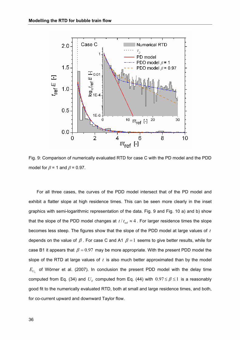
Fig. 9: Comparison of numerically evaluated RTD for case C with the PD model and
the PDD model for β = 1 and β = 0.97. 36
Fig. 10: Comparison of numerically evaluated RTD curves for case A1 (a) and B1 (b)
with the PD model and the PDD model for β = 1 and β = 0.97. 37
Fig. 11: Schematic representation of convolution procedure for a general case (top)
and for a unit cell of bubble train flow (bottom). 39
Fig. 12: Comparison of numerically evaluated RTD curves for case A2 (a) and B2 (b)
with the PD model and the PDD model. The dashed vertical lines correspond
to the delay time for each case. 43

vi
Fig. 13: Comparison of numerically evaluated RTD curves for Ncross=3 with
convolutions of the PD model and PDD model for (a) case A1 and (b) case
B1. The dashed vertical lines correspond to the delay time for each case. 45

vii
Nomenclature
Bo Bodenstein number
C Tracer concentration, mol/m3
csC Ratio between mean and maximum velocity in laminar flow through a channel
Ca Capillary number
Bd Bubble diameter at a certain axial position of the bubble, m
BD Maximum bubble diameter, m
filmd Thickness of liquid film between gas bubble and channel wall, m
hD Hydraulic diameter of channel, m
tracerD Molecular diffusion coefficient of tracer in liquid phase, m2/s
E Residence time distribution (RTD), 1/s
Eθ Non-dimensional RTD
UCEα Unit cell RTD for PDD model, 1/s
F Cumulative residence time distribution function
f Liquid volumetric fraction in a mesh cell
J Total superficial velocity, m/s
GJ Superficial velocity of gas phase, m/s
LJ Superficial velocity of liquid phase, m/s
axL Axial length of computational domain, m
refL Reference length scale, m
SL Liquid slug length, m
travelL Axial travelling distance of particles to determine the RTD, m
UCL Length of unit cell, m
x y z, ,L L L Physicals dimensions of computational domain, m
n Number of CSTRs or unit cells in series
crossN Number of times virtual particles must cross the domain to obtain the RTD
pN Number of particles
tN Number of time steps
viii
UCN Number of unit cells
Q Volumetric flow rate, m3/s
BRe Bubble Reynolds number
t Time, s
reft Reference time scale, s
t Mean residence time, s
Δt Time step width, s
classΔt Time interval of classes in the RTD, s
BU Bubble velocity, m/s
FU Mean velocity in liquid film and corner flow region in PDD model, m/s
LU Mean liquid velocity in the computational domain, m/s
L,filmU Mean velocity in the liquid film at a certain axial position, m/s
actL,maxU Actual maximum axial velocity in the liquid slug, m/s
thL,maxU Maximum axial velocity in fully developed Poiseuille flow, m/s
refU Reference velocity scale, m/s
V Volume, m3
Greek symbols
α Weighting factor in PDD model
β Pre-factor of bubble diameter for computation of FU in PDD model
δ Dirac delta function
ε Gas volume fraction in the unit cell
θ Dimensionless time, /t tθ ≡
λ Ratio act thL,max L,max/U U
μ Dynamic viscosity, Pa s
ρ Density, kg/m3
σ Coefficient of surface tension, N/m
2σ Variance of RTD, s2
ix
2θσ Non-dimensional variance of RTD
τ Mean residence time, s
Bτ Bubble break through time, s
Dτ Delay time, s
Fτ Mean residence time for liquid film and corner region in PDD model, s
hτ Mean hydrodynamic residence time, s
Sτ Mean residence time for liquid slug, s
Subscripts
B Bubble
F Liquid film
G Gas phase
L Liquid phase
p Particle
ref Reference value
S Liquid slug
UC Unit cell
Abbreviations
BTF Bubble Train Flow
CSTR Continuous Stirred Tank Reactor
PD Peak-Decay
PDD Peak-Decay-Decay
PFR Plug Flow Reactor
RTD Residence Time Distribution
UC Unit cell
WGO RTD model of Wörner, Ghidersa, Onea (2007)

x
Introduction
1
1. Introduction
Segmented gas-liquid flow is a common two-phase flow pattern in narrow channels. It is also
denoted as Taylor flow or bubble train flow (BTF) and consists of a sequence of elongated
bubbles which almost fill the entire channel cross section (Taylor bubbles). The individual
bubbles move along the channel while they are separated by liquid slugs. Bubble train flow is
of technical relevance, e.g. for miniaturized multiphase reactors (Jähnisch et al., 2000; Burns
& Ramshaw, 2001; Günther et al., 2004, Haverkamp et al., 2006) and for multiphase mono-
lith reactors (Roy et al., 2004; Kreutzer et al., 2005b, Bauer et al., 2005). While in an indus-
trial scale monolith reactors with Taylor flow are only used for production of H2O2 (Edvinson
Albers et al., 2001) they find increasing interest for potential use for Fischer-Tropsch synthe-
sis (De Deugd et al., 2003; Bradford et al., 2005; Güttel et al., 2008, Liu et al., 2009).
In real Taylor flow, the length of the liquid slugs and the size of individual bubbles
underlies variations. The variation of the bubble size results in a variation of the translational
velocity of individual bubbles. This may lead to coalescence and thus a further change of the
bubble size and slug length distribution. A useful abstraction of real bubble train flow is
perfect bubble train flow, where the bubbles are assumed to have identical size, shape and
velocity and where the length of all liquid slugs is the same. Then, the hydrodynamics of BTF
is fully described by a unit cell (UC) which consists of one bubble and one liquid slug.
An important characteristic of any chemical reactor is its residence time distribution
(RTD), since the RTD provides information about the flow and mixing behaviour of reaction
components (Levenspiel, 1999; Martin, 2000; Nauman, 2008). The knowledge of the RTD
and the kinetics of the chemical reaction is the basis for the design of any chemical reactor
since both determine the yield and selectivity of the reactor. This gives the motivation to
develop simple but yet reliable models that are able to predict the RTD in bubble train flow
from fluid properties and known integral flow parameters such as the superficial velocities of
the phases. Of major interest is the RTD of the continuous liquid phase, since the variation of
the residence time of the gas phase is small and its mean value can be computed by dividing

Introduction
2
the length of the channel by the bubble velocity. Desirable is a plug flow behaviour of the
liquid phase with a narrow RTD.
For the design and optimization of micro-structured reactors for process intensification
the ability to reliably predict the RTD is of great importance. Sun et al. (2008) recently
investigated the influence of the RTD on the synthesis of biodiesel in capillary micro-reactors
operated with Taylor flow. They found that the RTD in the micro-channel reactor was
remarkably decreased compared to the RTD which is required in batch systems to obtain a
high yield under the same reaction conditions. However, the RTD of the micro-reactors had
to be controlled to avoid the saponification of the biodiesel. Though this example
demonstrates the practical importance of the RTD, there are, unfortunately, only very few
experimental data on the liquid phase RTD available in literature for multiphase micro-
structured reactors such as monolith reactors. This may be attributed on one hand to the
difficulties of performing local measurements of the RTD in narrow channels and on the other
hand to the only recently increasing interest in this topic. As a consequence, reliable and
validated general models for the RTD in micro-structured reactors are missing. This is in
particular true for channels of non-circular cross-section, which are quite common in
monoliths and other micro-structured reactors. In rectangular channels, the film thickness at
the circumference of the bubble is not constant. As a consequence, a so-called corner flow
exists which makes the application of RTD models for circular channels invalid and requires
the development of refined models.
In experiments the residence time distribution is often measured by a stimulus-response
technique, where a specific quantity of a tracer (e.g. fluorescent substance, radionuclide,
solution of salt, etc.) is introduced at the system inlet as a short duration pulse or a step
function and where the time variation of the tracer concentration is recorded at the outlet.
The tracer particles injected at the inlet are assumed to follow the same paths through the
system as the original fluid particles they replaced. Thus, the tracer particles will have the
same distribution of residence times as the original fluid particles. By recording the times
when particles leave a histogram can be constructed. For a large sampling size this

Introduction
3
histogram converges to the differential residence time distribution function. This single-phase
flow approach can be applied to gas-liquid two-phase flows as well. The main difference is
that the system has now usually two inlets (one for the gas phase and one for the liquid
phase), while there is still one common outlet. To measure the residence time distribution of
the liquid phase in a gas-liquid flow, the tracer pulse is injected at the liquid inlet only.
The stimulus-response measurement technique is well suited for macro-reactors, where
the reactor volume is much larger than the volume of the tracer measurement device.
However, for micro-structured reactors, the reactor volume is usually smaller than the volume
of the measuring unit. This means that the residence time response of the tracer may already
be influenced by the measurement configuration itself. Measurements of liquid phase RTD
for two-phase flow through narrow channels are reported by Thulasidas et al. (1999) for
bubble-train flow in single straight channels (using a conductiometric technique), by Patrick
et al. (1995) for a monolith froth reactor (measuring the tracer concentration at the outlet with
a spectrometer), by Heibel et al. (2005) for film flow in a monolith reactor (using a dye tracer
and a spectrometer), by Yawalkar et al. (2005) and Kreutzer et al. (2005a) for bubble-train
flow in a monolith reactor (using a dye tracer and a spectrometer), by Bakker et al. (2005) for
a novel ‘open wall’ monolith reactor, by Kulkarni et al. (2005) for Taylor flow in a monolith
reactor (using a KCl tracer solution and a conductivity probe), and by Günther et al. (2004)
and Trachsel et al. (2005) for bubble-train flow in micro-fluidic channel networks of
rectangular cross-section (using a fluorescently labelled tracer pulse and a fluorescence
microscope). The latter authors showed that the residence time distribution of bubble-train
flow is very narrow as compared to single phase flow, which is a distinct advantage. Just
recently, Lohse et al. (2008) presented a novel method for determining the RTD in an
intricately structured micro-reactor, which employs a tracer ‘injection’ using the optical
activation of a caged fluorescent dye.
An alternative way to determine the RTD is by means of computational fluid dynamics
(CFD). There exist in principle two options to determine the residence time distribution from
CFD methods. The first one is the numerical simulation of the stimulus-response experiment,

Introduction
4
i.e. setting a short concentration pulse at the inlet of the computational domain, computing
the unsteady concentration field of the tracer within the computational domain and evaluating
it at the outlet. This approach has been used in a modified form by Salman et al. (2005,
2007) to determine the reactor residence time for Taylor flow in a circular micro-channel from
the residence time distribution of a single unit cell by using a convolution procedure. The
second possibility is the particle tracking method. Here, virtual particles are released at the
inlet and their trajectories are computed from the known velocity field of the CFD calculation.
A notable difference between the two methods is that in the particle method convective
properties of the flow are only monitored, while by evaluation of the unsteady concentration
field diffusive transport is additionally taken into account. The relative importance of
convective and diffusive transport is characterized by the Bodenstein number. For bubble-
train flow, it can be defined as B h tracer/Bo U D D≡ , where BU is the bubble velocity, hD is the
hydraulic diameter of the channel and tracerD is the molecular diffusion coefficient of the
tracer in the liquid phase. For a particle tracking method, no diffusion of the tracer is taken
into account. The RTD obtained by a particle tracking method is therefore representative for
an infinite value of the Bodenstein number.
To predict the residence time distribution for Taylor flow, Salman et al. (2004) developed
a numerical model valid for low values of the Bodenstein number. This model does not
account for the direction of gravity and assumes liquid slugs of uniform concentration and
liquid films around the bubble that can be adequately described by a one-dimensional
convection-diffusion equation. For large values of the Bodenstein number ( 10Bo > ) the
model can be simplified and an analytical solution is derived, which corresponds to the
representation of a unit cell by a tank-in-series model, consisting of a plug flow reactor (PFR)
and a continuous stirred tank reactor (CSTR). In a more recent paper, Salman et al. (2007)
numerically evaluated RTDs for a wide range of Bodenstein numbers (respectively Peclet
numbers) and compared it with predictions from three literature models (CSTR-PFR model,
two-region model of Pedersen & Horvath (1981), and the model of Thulasidas et al. (1999)).
They found that the shape of the RTD and the performance of the different models depend
Introduction
5
strongly on the parameter B film tracer/U d D , where filmd is the thickness of the liquid film
between the gas bubble and the channel wall.
Recently, Wörner et al. (2007) developed a new CFD-based method for evaluating the
liquid phase residence time distribution of bubble-train flow using data from direct numerical
simulations (DNS). The numerical simulations are performed for perfect bubble-train flow.
The method developed for evaluation of the RTD is a particle method and relies on the
uniform introduction of virtual particles in the volume occupied by the liquid phase within a
single flow unit cell. The residence time distribution is obtained by statistical evaluation of the
time required by virtual particles to travel axially the length of the unit cell, and by an
appropriate weighting procedure which takes into account the axial velocity at the initial
particle position. Residence time curves have been evaluated from DNS data of co-current
upward bubble-train flow in a square mini-channel of 2 mm × 2 mm cross section for values
of the capillary number in the range B L / 0.2 0.25Ca U μ σ≡ = − , where Lμ is the liquid
viscosity and σ is the coefficient of surface tension. The RTD curves obtained can be fitted
well by a simple exponential relationship, which has been developed on the basis of a
compartment model consisting of two tanks in series, the first tank being a plug flow reactor
and the second being a continuous stirred tank reactor. This model may be considered as
generalization of the model of Salman et al. (2004) which was developed for circular
channels, but cannot be applied adequately for square channels because of the corner flow.
Both, the model of Salman et al. (2004) and of Wörner et al. (2007) are derived for the
RTD of a unit cell. In practice, a single channel with bubble-train flow contains tens or
hundreds of unit cells depending on the length of the unit cell and the length of the channel.
Salman et al. (2007) computed the residence time of the capillary from the residence time of
the unit cell by means of a convolution method. Usually, a micro-structured reactor consists
of a large number of parallel channels. If the flow is evenly distributed across the different
channels, the RTD of the reactor is equal to that of a single channel. However, in practice the
flow rates through the different channels of the monolith reactor differ (Mantle et al., 2002),
Introduction
6
so that it is necessary to take this maldistribution effect into account when estimating the
reactor RTD from the single channel RTD.
The objective of the present report is twofold. First, we want to refine the unit cell RTD
model of Wörner, Ghidersa, Onea (2007) (the WGO model) for co-current upward bubble
train flow and develop a more general unit cell RTD model which is also valid for co-current
downward bubble train flow. Second, we want to develop a procedure to predict the RTD of
an arbitrary number of unit cells in series (i.e. the RTD of a single channel with perfect
bubble train flow) from the RTD of a single unit cell. In this report we investigate in how far
this can be done by a convolution procedure.
This report is organized as follows. In section 2 we introduce some fundamental aspects
and definitions of RTD theory. In section 3 we discuss issues related to the numerical
simulation of bubble train flow and to the numerical evaluation of the RTD. Section 4 is
devoted to the analytical modelling of the RTD for bubble train flow, namely the development
of a refined unit cell model and a model for multiple unit cells. In section 5 we present the
conclusions.

Fundamentals of residence time theory
7
2. Fundamentals of residence time theory
In this section we give a short introduction into fundamental aspects and definitions re-
lated to the concept of residence time distribution. Some passages in this section are
adopted from the English Wikipedia page for “residence time distribution” (accessed June,
2009). For further details we refer to text books, e.g. Fogler (1986) and Levenspiel (1999).
2.1. The residence time distribution
The residence time distribution (RTD) of a chemical reactor is a probability distribution
function that describes the amount of time that fluid elements spend inside the reactor. The
distribution of residence times is represented by an exit age distribution ( )E t . The function
( )E t has unit of time-1 and underlies the restriction
0
( )d 1E t t∞
=∫ (1)
The fraction of the fluid that spends a given duration t inside the reactor is given by ( )dE t t ,
while the fraction of fluid that leaves the reactor with an age less than 1t is
1
0
( )dt
E t t∫ (2)
The mean or average residence time is given by the first moment of the age distribution
0
( )dt t E t t∞
≡ ⋅∫ (3)
If there are no stagnant zones within the reactor then t will be equal to the mean hydrody-
namic residence time hτ , which is the residence time calculated from the total reactor vol-
ume V and the volumetric flow rate Q of the fluid
hVQ
τ ≡ (4)
The second central moment indicates the variance of the RTD and is given by
Fundamentals of residence time theory
8
2 2
0
( ) ( )dt t E t tσ∞
≡ −∫ (5)
The variance represents the square of the spread of the distribution as it passes the vessel
exit and has units of (time)2. It is particularly useful for matching experimental curves to one
of a family of theoretical curves (Levenspiel, 1999).
2.2. Measurement of the RTD
As discussed in the introduction of this report, residence time distributions are measured
by introducing a non-reactive tracer signal at the inlet and by measuring the time-dependent
tracer concentration at the outlet. The selected tracer should not modify the physical charac-
teristics of the fluid (equal density, equal viscosity) and the introduction of the tracer should
not modify the hydrodynamic conditions. In general, the tracer signal at the inlet will either be
a pulse or a step. Other functions are possible, but they require additional calculations to de-
convolute the RTD curve, ( )E t .
The pulse method requires the introduction of a very small volume of concentrated tracer
at the inlet of the reactor, such that it approaches the Dirac delta function. Although an
infinitely short injection cannot be produced, it can be made much smaller than the mean
residence time of the reactor. In the pulse method the RTD curve can be computed from the
measured time dependent tracer concentration ( )C t at the reactor outlet by the relation
0
( )( )( )d
C tE tC t t
∞=
∫ (6)
In the step method, the concentration of tracer at the reactor inlet is changed abruptly
from 0 to 0C . The concentration of tracer at the outlet is normalized to obtain the non-
dimensional curve
0
( )( ) C tF tC
= (7)
which increases monotonically from 0 to 1. The value of the mean residence time and the
variance can be computed from the function ( )F t by relations

Fundamentals of residence time theory
9
[ ]0
1 ( ) dt F t tτ∞
= = −∫ (8)
[ ]2 2
0
2 1 ( ) dt F t t tσ∞
= − −∫ (9)
The step- and pulse-responses of a reactor are related due to
0
( ) ( )dt
F t E t t= ∫ (10)
and
d ( )( )dF tE t
t= (11)
A step experiment is often easier to perform than a pulse experiment, but it tends to smooth
over some of the details that a pulse response could show. It is easy to numerically integrate
an experimental pulse response to obtain a very high-quality estimate of the step response,
but the reverse is not the case because any noise in the concentration measurement will be
amplified by numeric differentiation.
2.3. RTD of ideal reactors
The residence time distribution of a real reactor can be used to compare its behavior to
that of two ideal reactor models: the plug-flow reactor (PFR) and the continuous stirred-tank
reactor (CSTR). In an ideal PFR there is no mixing and the fluid elements leave in the same
order they arrived. Therefore, fluid entering the reactor at time t will exit the reactor at time
PFRt τ+ , where PFR PFRtτ = is the mean residence time of the plug-flow reactor. The residence
time distribution function is therefore a Dirac delta function
( )PFR( )E t tδ τ= − (12)
The variance of an ideal plug-flow reactor is zero.
An ideal CSTR is based on the assumption that the flow at the inlet is completely and
instantly mixed into the bulk of the reactor. The reactor and the outlet fluid have identical
Fundamentals of residence time theory
10
homogeneous compositions at all times. An ideal CSTR has an exponential residence time
distribution
CSTRCSTR CSTR
1( ) exp tE tτ τ
⎛ ⎞= −⎜ ⎟
⎝ ⎠ (13)
Here, CSTR CSTRtτ = is the mean residence time of the continuous stirred-tank reactor. The
variance of the CSTR is 2 2CSTR CSTRσ τ= . The RTD for a cascade consisting of n∈ identical
CSTRs in series is
1
CSTRCSTR CSTR
( ) exp( 1)!
n
n n
t tE tn τ τ
− ⎛ ⎞= −⎜ ⎟− ⎝ ⎠
(14)
2.4. Non-dimensional RTD
For comparing different reactors it is useful to introduce a non-dimensional RTD curve
( ) ( )E t E tθ θ ≡ ⋅ (15)
which is a function of a dimensionless time
tt
θ ≡ (16)
The non-dimensional mean value of Eθ is then
0 0 0
1 1( )d ( ) d ( )d 1tE t E t t t E t tt t tθθ θ θ θ
∞ ∞ ∞
≡ ⋅ = ⋅ ⋅ = ⋅ =∫ ∫ ∫ (17)
while the non-dimensional variance is 2 2 2/ tθσ σ= .
For a single CSTR it is
CSTR ( ) exp( )E θ θ= − (18)
and 2,CSTR 1θσ = . The mean residence time for a series of n identical CSTRs is
CSTR CSTRn nτ τ= . With definition of the non-dimensional time
CSTRCSTR CSTR
nn
t tn
θτ τ
≡ = (19)
we can write Eq. (14) in the non-dimensional form

Fundamentals of residence time theory
11
( )1
CSTRCSTR CSTR CSTR
( )( ) exp( 1)!
nn
n n nn nE n
nθθ θ
−
= −−
(20)
The non-dimensional variance of a series of n identical CSTRs is
2 1nθσ = (21)
For real reactors, often the mean residence time τ and the variance 2σ are measured and
the reactor RTD is modelled as a series of n CSTRs, where n is computed from Eq. (22)
2
2 2
1nθ
τσ σ
= = (22)
2.5. Definitions for the unit cell RTD in bubble train flow
We now introduce some definitions for the RTD in bubble train flow, which we will need
later in this report. We consider a perfect bubble train flow consisting of a cascade of n iden-
tical unit cells in series featuring RTD UC ( )nE t . The mean residence time of this RTD is
UC UC UC0
( )dn n nt t E t tτ∞
≡ = ⋅∫ (23)
and the variance is
2 2UC UC UC
0
σ ( ) ( )dn n nt t E t t∞
= −∫ (24)
We define the non-dimensional time
D DUC
nUC UCn
t n t nn
τ τθτ τ− −
≡ = (25)
Here, Dτ is the delay time which will be defined later and UCτ is the mean residence time of
a single unit cell. We define the non-dimensional form of the RTD UC ( )nE t as
, UC UC UC UC( ) ( )n n nE n E tθ θ τ≡ (26)
The mean hydrodynamic residence time for a series of n unit cells in bubble train flow is
UCh
L
nn
VQ
τ = (27)
Fundamentals of residence time theory
12
Here, UC UC chnV nL A= is the volume of a domain with n unit cells of length UCL , L L chQ J A= is
the liquid volumetric flow rate, LJ is the liquid superficial velocity and chA is the cross-
sectional area of the channel. Therefore, Eq. (27) gives
UCh
Ln
nLJ
τ = (28)
Numerical simulation of bubble train flow
13
3. Numerical simulation of bubble train flow
In this section, we first give a short overview on the numerical method and the computer
code used to perform the direct numerical simulations of the bubble-train flow. We then de-
scribe the simulation set-up and give the physical and numerical parameters of the simula-
tions. Finally, we shortly present the method for evaluation of the RTD from the DNS data
and present some visualizations of the local residence time field.
3.1. Numerical method
The direct numerical simulations are performed with the in-house computer code TUR-
BIT-VOF (Sabisch 2000, Sabisch et al. 2001), which solves the single-field Navier-Stokes
equations with surface tension term for two incompressible immiscible fluids under assump-
tion of constant fluid properties (i.e. density, viscosity, surface tension). The single-field for-
mulation automatically accounts for the proper momentum jump conditions across the gas-
liquid interface. The governing equations are written in non-dimensional form, see Ghidersa
et al. (2004) and Öztaskin et al. (2009). For normalization, a reference length scale refL and
reference velocity scale refU are used, which need to be specified. The solution strategy is
based on a projection method, where the resulting Poisson equation for the pressure is
solved by a conjugate gradient solver. Time integration of the single field Navier-Stokes
equation is done by an explicit third order Runge-Kutta method. Discretization in space is
based on a finite volume method, where a regular Cartesian staggered grid is used. All de-
rivatives in space are approximated by second order central differences.
For computing the evolution of the deformable interface, which separates the two
immiscible fluids, the volume-of-fluid (VOF) method is used. In any mesh cell that
instantaneously contains both phases, the interface is locally approximated by a plane. The
orientation and location of the plane is reconstructed from the discrete distribution of the
volumetric fraction f of the continuous fluid. Note that - for a certain instant in time - we
have 1f = for mesh cells entirely filled with liquid, 0f = for mesh cells entirely filled with
gas, and 0 1f< < for mesh cells that contain both phases. The evolution of f is governed
Numerical simulation of bubble train flow
14
by an advection equation, which expresses the mass conservation of the continuous phase.
To avoid any smearing of the interface, this f -equation is not solved by a difference
scheme. Instead, the flux of f across the faces of any interface mesh cell is calculated in a
geometrical manner, depending on the location and orientation of the plane representing the
interface. For further details about the numerical method we refer to Sabisch et al. (2001)
and Öztaskin et al. (2009). We also note that a comprehensive code-to-code comparison
exercise of TURBIT-VOF with three major commercial CFD codes was performed for bubble-
train flow in a square mini-channel, see Özkan et al. (2007).
3.2. Simulation set-up
The set-up of the simulations is described in detail in Ghidersa et al. (2004) and Wörner
et al. (2007) and is therefore only shortly repeated here. We consider a computational do-
main and co-ordinate system as displayed in Fig. 1. No-slip boundary conditions are applied
at the four side walls of the square channel, while in (vertical) axial direction ( y ) periodic
boundary conditions are used. The length of the computational domain in axial direction is
axL . This length may represent one unit cell as displayed in Fig. 1, or may represent ucN unit
cells, where ucN is a positive integer. The flow can be co-current upward or downward, de-
pending on the sign of the specified driving axial pressure drop across the computational
domain. The simulations start from fluid at rest with a bubble placed in the centre of the com-
putational domain. They are continued in time until the bubble velocity and the mean liquid
velocity within the computational domain obey constant terminal values.
3.3. Simulation parameters
In the present report five different cases are considered. For all cases the following pa-
rameters are used: h x z ref 2mmD L L L= = = = , liquid density 3L 957 kg/mρ = , gas density
3G 11.7 kg/mρ = , liquid viscosity L 0.048 Pa sμ = ⋅ , gas viscosity G 0.184 mPa sμ = ⋅ , coeffi-
cient of surface tension 0.02218 N / mσ = , reference velocity ref 0.0264m/sU = , reference
time scale ref ref ref/ 0.0757st L U≡ = and gas holdup in the computational domain 33%ε ≈ .

Numerical simulation of bubble train flow
15
Fig. 1: Sketch of computational domain and co-ordinate system.
The cases differ with respect to the length of the unit cell, UCL , the number of unit cells in
the domain, ucN , and the flow direction, see Tab. 1. For cases A1, B1 and C the
computational domain contains one unit cell only, while it contains two unit cells for cases A2
and B2. Case A1 and B1 correspond to case A2 and E, respectively, in Wörner et al. (2007).
Cases A2 and B2 correspond to case A1 and B1, respectively, in Öztaskin et al. (2009).
While in all these cases the flow is co-current upward, it is co-current downward for case C,
which is otherwise similar to case G in Wörner et al. (2007). Further data given in Tab. 1 are
the time step width tΔ and the number of computes times steps tN . In all cases a uniform
grid of mesh size ref / 48x y z LΔ = Δ = Δ = is used.

Numerical simulation of bubble train flow
16
Tab. 1: Numerical parameters of the simulations
Case Domain Grid ax ref/L L UCN ε tN refΔ /t t
A1 1×1×1 48×48×48 1.0 1 0.3307 40 000 52.5 10−×
A2 1×2×1 48×96×48 2.0 2 0.3307 50 000 52.5 10−×
B1 1×1.5×1 48×72×48 1.5 1 0.3303 50 000 52.5 10−×
B2 1×3×1 48×144×48 3.0 2 0.3303 70 000 52.5 10−×
C 1×1.75×1 48×84×48 1.75 1 0.3303 45 000 51.5 10−×
In Tab. 2 for each case terminal values of characteristic velocities and bubble dimensions as
well as the bubble Reynolds number B L h B L/Re D Uρ μ≡ and capillary number
L B /Ca Uμ σ≡ are given. For all cases the bubble is axi-symmetric, i.e. its cross-section at
any axial position is circular.
Tab. 2: Terminal values of velocities, bubble dimensions, mean hydrodynamic res-
idence time, bubble Reynolds number and capillary number for the different cases.
Case B ref/U U L ref/U U ref/J U B h/D D S h/L D h ref/ tτ BRe Ca
A1 3.66 1.20 2.02 0.809 0.064 1.245 3.86 0.21
A2 3.66 1.20 2.02 0.809 0.064 1.245 3.86 0.21
B1 3.86 1.37 2.19 0.849 0.292 1.635 4.06 0.22
B2 3.96 1.37 2.22 0.843 0.280 1.635 4.17 0.23
C -3.25 -1.53 -2.09 0.891 0.480 1.708 3.42 0.19
3.4. Procedure for numerical evaluation of the RTD from DNS data
The procedure for the numerical evaluation of the RTD of the liquid phase within a unit
cell of the bubble train flow is described in detail in Wörner et al. (2007). Here, we give a
short overview on key issues of this evaluation procedure. The method relies on data for the
instantaneous three-dimensional velocity and volume fraction field within a unit cell which
have to be obtained in advance by a direct numerical simulation (DNS). The evaluation
Numerical simulation of bubble train flow
17
procedure is only useful for fully developed bubble train flow, where the translational velocity
of the bubble is constant and the bubble shape is steady. The method to evaluate the RTD
from the DNS data is a particle tracking method and relies on the uniformly spaced
introduction of virtual particles in the volume occupied by the liquid phase within a single flow
unit cell. The position of each particle within the given flow field is tracked by a first order
Euler scheme, in which the velocity field at the particle position is obtained from linear
interpolation from the staggered DNS grid. The residence time distribution is obtained by a
statistical evaluation of the time needed by virtual particles to travel an axial distance
equivalent to the length of the unit cell, and by an appropriate weighting procedure which
takes into account the axial velocity at the particle’s initial position.
There exist three numerical parameters for evaluation of the RTD. The first one is the
particle Courant-Friedrich-Levy (CFL) number
p pp
tCFL
xΔ
≡Δ
u (29)
which is used to determine the time step width ptΔ for the particle tracking. Here, the CFL
number is 0.2 for all cases. The second parameter is the number of particles per unit length
pN . This parameter defines the initial positions of the particle set, as it constitutes the dis-
tance between neighbouring particles in the three coordinate directions. Here, we use
p 48N = for all cases. The third parameter is classΔt . It is used to subdivide the time axis in
certain intervals of size classΔt . Each time interval is denoted as a class. The RTD is obtained
by sorting the residence time of all particles in classes and by subsequent normalization of
the resulting histogram. In Fig. 2 a) we illustrate the influence of the choice of classtΔ on the
numerically evaluated RTD. Three different values of classtΔ are used for evaluation of the
RTD for case C, namely class D / 3t τΔ = , D / 2τ and Dτ . It appears that values of classtΔ may
result in quite different values of E in neighbouring classes while large values of classtΔ lead
to smoother curves but have a coarser resolution. In Fig. 2 a) one may also recognise that
the area of the first three classes with class D / 3t τΔ = , the area of the first two classes with
class D / 2t τΔ = and the area of the first class for class Dt τΔ = are all equal. However, the choice

Numerical simulation of bubble train flow
18
of classtΔ has a large influence on the height of the peak of the RTD at Dt τ≈ . This makes a
comparison of models for the RTD with the numerical evaluated RTD difficult.
A particle that leaves the computational domain through one of its two faces with periodic
boundary conditions re-enters it through the opposite face. Thus a particle may travel an ax-
ial distance that is larger than the axial size of the computational domain axL . We denote the
the axial distance that any virtual particle must travel before its residence time is recorded by
travelL and define cross travel ax/N L L≡ . Thus, crossN allows evaluating the RTD of a series of mul-
tiple virtual unit cells. To test if this procedure is adequate to determine the RTD of multiple
unit cells we applied it to cases A1 and A2. Both cases have an identical unit cell. However,
in case A1 the computational domain contains one unit cell while it contains two unit cells in
case A2. In Fig. 2 b) we compare the RTD for case A1 and cross 2N = with the RTD for case
A2 and cross 1N = . The differences between both RTDs are very small. Therefore we con-
clude that the RTD for a number of n unit cells in series can be determined from simulation
results with one unit cell in the computational domain by setting crossN equal to n .
3.5. Analysis of local residence time field
From evaluation of the three-dimensional direct numerical simulation data the three-
dimensional field of the local residence time in the liquid phase of the bubble train flow is
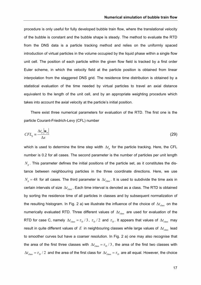
obtained. Fig. 3 shows a visualization of this field for case B1 and also displays the
computed bubble shape (note the periodic boundary conditions in axial direction). In this
figure, the local residence time in the computational domain is shown for two different planes,
once for a mid-plane in vertical axial direction ( y ) and once for a horizontal channel cross-
section. The different values of the residence time are represented by a colour code. The
figure indicates that fluid elements in the central region of the liquid slug have the shortest
residence time, i.e. travel fastest along the channel. In general, the residence time is small
for liquid fluid elements close to the bubble and is large for liquid fluid elements close to the
solid walls. As expected, the highest values of the residence time are found in the four
corners of channel.

Numerical simulation of bubble train flow
19
Fig. 2: a) Illustrations of influence of Δtclass on the numerically evaluated RTD curve. b)
Comparison of RTD curves for two unit cells, obtained from case A1 with Ncross=2 and from
case A2 with Ncross=1.
Numerical simulation of bubble train flow
20
Fig. 3: Visualization of the bubble shape and contour plot of the local non-dimensional resi-
dence time ref/t t in two different planes for case B1.

Modelling the RTD for bubble train flow
21
4. Modelling the RTD for bubble train flow
4.1. The RTD for a single unit cell
4.1.1. The WGO model
The RTD curves in Fig. 2 show a characteristic behaviour. For small values of t the RTD
is zero. At the so called “delay time” Dτ the RTD becomes positive. The delay time of the
RTD may thus be modelled by a plug flow reactor. For Dt τ> the RTD strongly increases to
the highest value and then slowly decays. The sudden increase of the RTD from zero to the
highest value corresponds to the residence time of the fastest fluid particles, i.e. the liquid
slug region in Fig. 3. The semi-logarithmic scale of the inset graphics shows that the slope of
the RTD at small and medium time is almost constant. This suggests that this part of the
RTD curve may be approximated by an exponential relationship. Thus, the RTD curve may
be approximated by a (single-phase flow) compartment model consisting of two tanks in
series. The first tank is a plug flow reactor (PFR) which represents the delay time and the
second tank is a continuous stirred tank reactor (CSTR) which represents the exponential
decay, see Fig. 4. The delay time is determined by the minimum time of fluid elements to
pass the channel, whereas the height of the peak and the slope of the exponential decay are
determined by the ratio of flow rate to tank volume /Q V (see Fig. 12.1 in Levenspiel, 1999).
This PFR-CSTR in series concept has already been adopted by Salman et al. (2004) to
develop an analytical model for predicting axial mixing during Taylor flow in micro-channels
at low Bodenstein numbers. However, this model was developed for circular channels where
the film thickness is uniform and showed deficiencies for non-circular channels where the film
thickness is not uniform (Wörner et al., 2007).
For co-current upward bubble train flow in a square channel, Wörner et al. (2007)
proposed two slightly different models. The first model denoted as JE is given by
UC B
J UC UCUC B
UC UC B
0 for /
( )exp for /
t L U
E E t LJ J t t L UL L U
<⎧⎪
⎡ ⎤= = ⎛ ⎞⎨ − ≥⎢ ⎥⎜ ⎟⎪⎝ ⎠⎣ ⎦⎩
(30)

Modelling the RTD for bubble train flow
22
In this model, the CSTR corresponds to the liquid slug region, which is well mixed because of
the fluids recirculating motion (Thulasidas et al., 1997). The mean velocity in the liquid slug is
equal to the total superficial velocity J which is given by G L B L(1 )J J J U Uε ε≡ + = + − .
Here, LU is the mean liquid velocity and ε is the gas volume fraction in the unit cell. The
mean residence time of the CSTR is, therefore, in this model given by CSTR S UC /L Jτ τ= = .
The model LUE is obtained from Eq. (30) by replacing the superficial velocity J by the mean
liquid velocity LU . In the following we will consider only model JE and denote it as WGO
model (Wörner, Ghidersa, Onea 2007).
Fig. 4: Compartment representation of the WGO model. QL is the volumetric flow rate of the
liquid phase and VPFR and VCSTR are the volume of the plug flow reactor and the continuous
stirred tank reactor, respectively.
Modelling the RTD for bubble train flow
23
In the WGO model, the delay time is taken to be the bubble break-through time
B UC B/L Uτ ≡ , which is the time the bubble needs to move an axial distance equivalent to
UCL . The mean residence time of the CSTR representing the liquid slug is S UC /L Jτ ≡ . With
these definitions one can write Eq. (30) in the compact form
B BJ UC
S S
( )( ) expτ ττ τ
⎛ ⎞− −= = −⎜ ⎟
⎝ ⎠
H t tE E t (31)
Here,
0 for 0( )
1 for 0x
H xx<⎧
= ⎨ ≥⎩ (32)
is the Heaviside step function. The argument of this discontinuous function determines the
delay time of the RTD, i.e. the time needed by the fastest particles to cross the reactor. The
integral of Eq. (31) from zero to infinity is unity and thus satisfies the necessary conditions of
any RTD, see Appendix A.1.1.
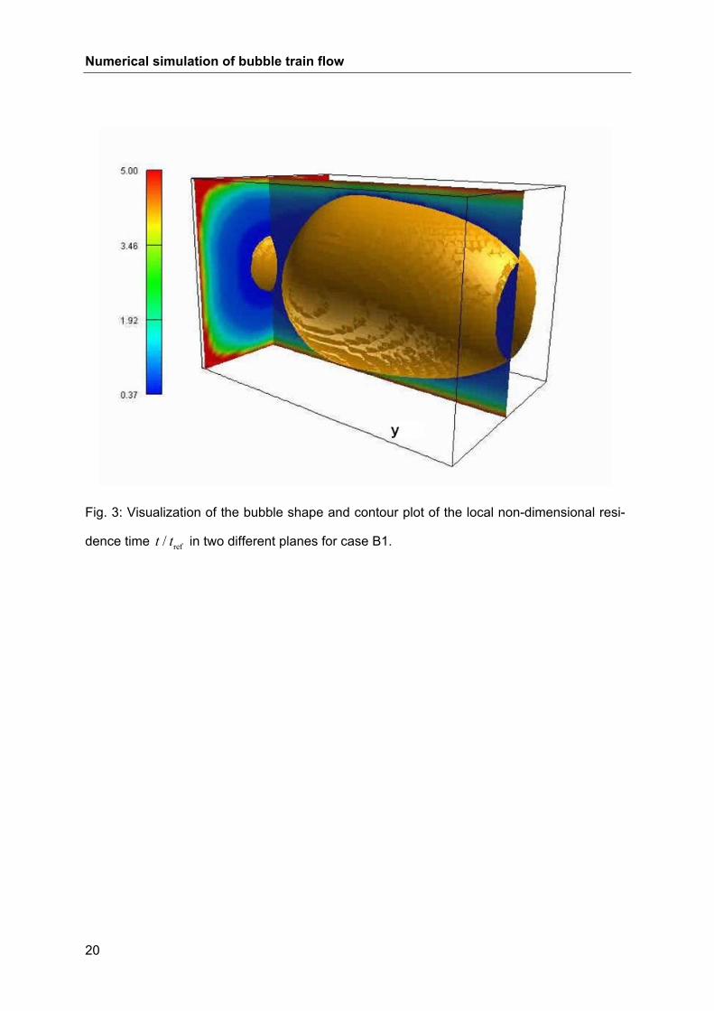
In Tab. 3 we list the values of Bτ and Sτ which are used in the WGO model for the dif-
ferent cases. Also given are the values for class refΔ /t t that will be used for each case.
Tab. 3: Values of parameters for unit cell RTD models.
Case refB / tτ refS / tτ actL,max ref/U U th
L,max ref/U U λ refD / tτ class refΔ /t t
A1 0.273 0.497 3.66 4.22 0.867 0.273 0.133
A2 0.273 0.497 3.64 4.22 0.863 0.275 0.133
B1 0.389 0.684 4.02 4.59 0.876 0.373 0.186
B2 0.379 0.674 4.08 4.66 0.876 0.367 0.183
C 0.539 0.836 -3.89 -4.39 0.879 0.450 0.225

Modelling the RTD for bubble train flow
24
4.1.2. The PD and PDD model
In this section, we develop two improved models for the RTD of a unit cell. The new
models will refine the WGO model with respect to the delay time and with respect to the
slope of the RTD at high values of t (i.e. the “tail” of the RTD).
4.1.2.1. Delay time
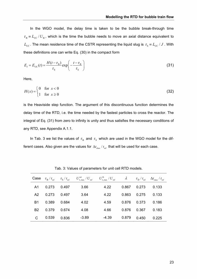
In Fig. 5 we compare the unit cell RTD model with the numerically evaluated RTD curves
for case A1 and case C. In the figure, the shaded area represents the numerically evaluated
RTD and the solid line the approximation by the WGO model. The dashed vertical lines de-
note the bubble break-through time. From Fig. 5 (a), where the dashed line agrees with the
delay time of the RTD, we see that no fluid particles are moving faster than the bubble and
most of the fluid particles are moving with a velocity that is only slightly smaller than the bub-
ble velocity. However, for downward flow we see from Fig. 5 (b) that some particles need
less time than the bubble to pass the channel. This means that the velocity of some fluid par-
ticles is higher than the bubble velocity. To investigate the reason for this we analyze next
the local flow field in upward and downward bubble train flow.
Fig. 6 shows visualisations of the computed bubble shape and velocity fields for co-
current upward flow (case G in Wörner et al., 2007) and for co-current downward flow
(present case C). In the left half of the figure the velocity field in the vertical axial mid-plane is
shown in the fixed frame of reference, while in the right half it is displayed in the frame of
reference moving with the bubble (i.e. BU is subtracted from the vertical velocity
component). For both cases, the velocity in the liquid film region is almost zero as indicated
in the fixed frame of reference. In the moving frame of reference, the velocity is almost zero
in the rear part of the bubble for the upward case. These blank regions, which are visible in
the right half of Fig. 6 a), indicate that part of the liquid slug that is moving approximately with
the bubble velocity BU . Hence, to consider the bubble velocity as representative for the
fastest tracer particles and to use the bubble break-through time in the unit cell RTD model is
reasonable for this upward flow case.
Modelling the RTD for bubble train flow
25
Fig. 5: Comparison of numerically evaluated unit cell RTD with the WGO model for (a) case
A1 and (b) case C. The dashed vertical line indicates the bubble break-through time for
each case.

Modelling the RTD for bubble train flow
26
a) b)
Fig. 6: Computed bubble shape and velocity field in vertical mid-plane z = 1 mm for fixed
frame of reference (left half) and for frame of reference linked to the bubble (right half) for (a)
co-current upward flow (case G in Wörner et al., 2007) and (b) co-current downward flow
(case C).
However, for the downward case C the velocity vectors in the liquid slug behind the
bubble have a finite length in the moving frame of reference; see the right half of Fig. 6 b).
This indicates that the velocity of that part of the liquid slug is higher than the bubble velocity,
which is consistent with the RTD displayed in Fig. 5 (b). This behaviour can be explained by
the buoyancy force, which accelerates the bubble relative to the liquid for co-current upward
flow but retards it for co-current downward flow. Thus, in the downward flow regime liquid
fluid elements may be faster than the bubble. In the RTD model, therefore, in Eq. (30) the
bubble velocity should be replaced by the maximum velocity in the liquid slug in order to
obtain a more general model which is also valid for downward flow.

Modelling the RTD for bubble train flow
27
For any fully developed laminar flow through a straight channel there exists a linear
relationship between the mean and maximum velocity, i.e. mean cs maxU C U= . The value of the
constant csC depends only on the shape of the channel cross-section and is cs 0.5C = for a
circular channel and cs 1/ 2.0962 0.477C = = for a square channel (Shah and London, 1978).
In bubble train flow, the mean liquid velocity within the liquid slug is given by L,meanU J= .
Thus, if the liquid slug is long enough to be fully developed, we have thL,max cs/U J C= . For
shorter liquid slugs the actual maximum velocity in the liquid slug may be smaller, say
act thL,max L,maxU Uλ= where λ is in the range 0 1λ< ≤ .
Fig. 7: Wall-normal profiles of magnitude of axial velocity in a horizontal cross-section
through the middle of the liquid slug for case A1, B1, and C. For each case the velocity pro-
file is normalized by the respective bubble velocity. The horizontal lines denote the normal-
ized maximum velocity of a fully developed Poiseuille profile for each case.

Modelling the RTD for bubble train flow
28
In Fig. 7 we show the profile of the magnitude of the axial velocity in the middle of the
liquid slug for case A1, B1 and C. In this figure, the horizontal lines denote the maximum
velocity in a fully developed laminar flow with the same flow rate for each case. Fig. 7 shows
that in the present simulations the liquid slug is too short to become fully developed. I.e. the
profiles are not parabolic but rather flat for all cases. This supports the experimental finding
of Thulasidas et al. (1997) and Tsoligkas et al (2007). The latter authors investigated the
liquid velocity profiles in the centre of the liquid slug of a co-current downward Taylor flow in
a square mini-channel and found that short liquid slugs with S hL D< exhibited a flat axial
velocity profile while long slugs with S hL D> have a parabolic one. Obviously, in short slugs
the velocity field is not fully developed. Thulasidas et al. (1997) found that in their
experiments the Poiseuille profile within the liquid slug is fully developed for S h/ 1.5L D ≥ .
Therefore, λ must increase with increasing slug length and asymptotically approach unity
when the flow is fully developed. The values of act thL,max L,max/U Uλ = in the present simulations
are given in Tab. 3. For all cases λ is in the range 0.86−0.88.
Fig. 7 also shows that for case A1, by incident, the maximum velocity actL,maxU just equals
the bubble velocity. For case B1, where the liquid slug is somewhat longer than in case A1,
the maximum velocity actL,maxU is somewhat larger than BU . For case C with a co-current
downward flow, actL,maxU is clearly higher than BU . Additionally, the velocity profile tends to
become more parabolic. These results also elucidate the relation between the bubble break-
through time and the delay time. To use the bubble break-through time as delay time may be
reasonable only for upward flow with very short liquid slug lengths like case A1 and A2,
where actL,max BU U≈ . This is, however, not valid for case C, where act
L,maxU is much larger than
BU , and therefore Bτ is larger than Dτ . Thus, it is necessary to refine the WGO model with
respect to the delay time, to yield a more general and consistent model for any flow direction
and any length of the liquid slug.
To refine the WGO model for co-current downward bubble train flow with an arbitrary
length of the liquid slug we replace in Eq. (30) the bubble velocity BU by
act thL,max L,max cs/U U J Cλ λ= = . This yields the following model:

Modelling the RTD for bubble train flow
29
cs UC
UC cs UCcs UC
UC
0 for / ( )( )
exp for / ( )
λ
λλ
<⎧⎪= ⎛ ⎞⎨ − ≥⎜ ⎟⎪ ⎝ ⎠⎩
t C L JE t C LJ t t C L J
L J (33)
This revised WGO model is more general since it takes the velocity of the fastest fluid parti-
cles to compute the delay time instead of the bubble velocity. Here, the delay time is
uc uc cs uc csD Sact th
L,max L,max
L L C L CU U J
τ τλ λ λ
≡ = = = (34)
The revised WGO model for a single unit cell can then be written in the compact form
csD D DUC
S S S S
( ) ( )( ) exp exp CH t t H t tE t τ τ ττ τ τ λ τ
⎛ ⎞ ⎛ ⎞− − −= − = −⎜ ⎟ ⎜ ⎟
⎝ ⎠ ⎝ ⎠ (35)
In the following, we denote this model as PD model. Here P stands for “peak” and D for “de-
cay”. This name reflects that the RTD consists of one peak followed by an exponential de-
cay. In the PD model λ is unknown yet. However, λ is a function of S h/L D and should ap-
proach unity for large values of S h/L D . Here, we take the values of λ as given in Tab. 3
while the development of a suitable relationship for S h( / )L Dλ λ= will be a future task for us.
For the mean residence time of the RTD in Eq. (35), we obtain the result
csUC UC UC D S S
0
( )d 1Ct tE t tτ τ τ τλ
∞ ⎛ ⎞≡ = = + = +⎜ ⎟⎝ ⎠∫ (36)
(see Appendix A.1.2). The variance is given by
2 2UC Sσ τ= (37)
(see Appendix A.1.3). Introducing the non-dimensional time
DUC
UC
t τθτ−
≡ (38)
we can write Eq. (35) in the compact non-dimensional form
( )
UC UC,UC UC UC UC UC UC
S S
D S D SD S UC UC
S S
( ) ( ) exp
( ) exp
E E t H
H
θτ ττ τ θ θτ τ
τ τ τ ττ τ θ θτ τ
⎛ ⎞≡ = −⎜ ⎟
⎝ ⎠⎛ ⎞+ +
= + −⎜ ⎟⎝ ⎠
(39)
Modelling the RTD for bubble train flow
30
4.1.2.2. Tail of the RTD
The tails of the RTDs in Fig. 5 correspond to the flow in the liquid film which is almost
stagnant (see velocity profiles in the left half of Fig. 6). The inset graphic in Fig. 5 shows the
numerical and modelled RTD in a semi-logarithmic representation. This allows for an easy
visual comparison of the slopes of both RTDs. The numerical RTD shows two slopes, a
steeper one for ref/ 4t t < and flatter one for ref/ 4t t < . In contrast, the slope of the WGO
model is constant and the tail of the RTD is not accurately represented by this model. In
Wörner et al. (2007), the steeper RTD slope for ref/ 4t t < is better fitted by model JE since
residence times ref/ 4t t < correspond mainly to fluid elements in the liquid slug, where the
mean velocity is equal to J . However, the flatter slope for ref/ 4t t > is better approximated
by model LUE . This is because residence times ref/ 4t t > correspond to fluid elements in the
four corners of the channel. There, the mean liquid velocity is smaller than J and may be
approximated by the mean liquid velocity in the unit cell LU . Though LUE is a better
approximation for ref/ 4t t > , the slope of this model is still too steep for high residence times
(see Fig. 8 a in Wörner et al., 2007). Hence, an even lower mean liquid velocity should be
chosen for the corner flow to cause a flatter slope for high residence times.
Considering these ideas, the WGO model respectively the PD model shall be developed
further towards a model which yields two different slopes for small and large times in order to
represent the tail of the RTD more accurately. For this purpose, Wörner et al. (2007) sug-
gested the three tank compartment model as displayed in Fig. 8. This model consists of a
PFR that is in series with two CSTRs in parallel. The RTD of this compartment model is cha-
racterized by a peak which is followed by the superposition of two exponential decays with
different slopes (see Fig. 12.1 in Levenspiel, 1999). We will, therefore, denote this model as
PDD model (peak-decay-decay). In the PDD model one CSTR corresponds to the liquid
slug, while the second corresponds to the flow in the liquid film and the corners. Since both
CSTRs are in parallel, the resulting RTD is the sum of two exponentials. The slopes of both
exponentials are determined by the mean residence time of the liquid slug Sτ and by the
mean residence time of the CSTR representing the liquid film /corner flow, respectively.

Modelling the RTD for bubble train flow
31
Fig. 8: Compartment representation of the PDD model. QL is the volumetric flow rate of the
liquid. VPFR is the volume of the plug flow reactor while VS and VF denote that of the continu-
ous stirred tank reactor, respectively. The subscripts ‘S’ and ‘F’ correspond to the liquid slug
and the liquid film / corner flow, respectively.
A relation for L,FQ can be obtained from a liquid mass balance in a frame of reference
moving with the bubble. We consider a control volume that consists of an axial portion of the
channel where one end is in the liquid slug and the other end is in the bubble region. Then a
balance of the liquid inflow and outflow flow rates yields
( )B ch L,film B ch B( )( )J U A U U A A− = − − (40)
so that
( ) chL,film B B
ch B
AU U U JA A
= − −−
(41)

Modelling the RTD for bubble train flow
32
In this equation, L,film L,film ( )U U y= and B B ( )A A y= represent the mean axial liquid velocity
and bubble cross-sectional area, respectively. The position y denotes the control volume
outlet and is variable. The liquid volumetric flow rate in the outflow cross-section of the con-
trol volume is then given by
( ) ( ) ( )chL,film L,film ch B B B ch B ch B B
ch B
AQ U A A U U J A A JA U AA A
⎡ ⎤= − = − − − = −⎢ ⎥−⎣ ⎦
(42)
As pointed out by Abiev (2008), the sign of L,filmU and L,fQ can be positive or negative.
For an axi-symmetric bubble with local cross-sectional diameter B ( )d y one obtains from
Eq. (41) the result
( )12
BL,film B B
h
14
dU U U JD
π−
⎡ ⎤⎛ ⎞⎢ ⎥≡ − − − ⎜ ⎟⎢ ⎥⎝ ⎠⎣ ⎦
(43)
This relation is very sensitive to the value of Bd . Here, we are interested in the mean liquid
velocity in the axial cross-section where the bubble diameter is largest. Thus, we take
B Bd Dβ= and compute the mean liquid velocity in the liquid film / corner region from relation
( )12
BF B B
h
14
DU U U JDβπ
−⎡ ⎤⎛ ⎞⎢ ⎥≡ − − − ⎜ ⎟⎢ ⎥⎝ ⎠⎣ ⎦
(44)
In the sequel, we consider two different values for β , namely 1β = and 0.97β = . In Tab. 4
we list the values of FU that are obtained from this equation for the different cases for both
values of β . Our RTD model is only reasonable if FU has the same sign as J , i.e. is posi-
tive for upward flow and negative for downward flow. Then, the mean residence time of the
CSTR representing the liquid film is computed from F UC F/L Uτ ≡ while that of the CSTR
representing the liquid slug is the same as in the WGO and PD model, namely S UC /L Jτ ≡ .
For the moment, we define the relation between the flow rates L,SQ and L,FQ in the two
CSTRs by a weighting factor L,S L,S L,F/ ( )Q Q Qα = + . This weighting factor is in the range
0 1α< ≤ and will be determined later. In section 4.2 where we consider multiple unit cells,
we always assume that all unit cells are identical so that the value of α is the same.

Modelling the RTD for bubble train flow
33
The RTD of the three tank compartment model is then given by
UC ( ) 0E tα = (45)
for actUC L,max/<t L U , and by
UC UCF FUC act act
L,max L,maxUC UC UC UC( ) exp (1 ) expL LU UJ JE t t t
L L U L L Uα α α
⎡ ⎤ ⎡ ⎤⎛ ⎞ ⎛ ⎞⎢ ⎥ ⎢ ⎥⎜ ⎟ ⎜ ⎟
⎜ ⎟ ⎜ ⎟⎢ ⎥ ⎢ ⎥⎝ ⎠ ⎝ ⎠⎣ ⎦ ⎣ ⎦= − + − − (46)
for actUC L,max/≥t L U . Introducing the delay time act
D uc L,max/L Uτ ≡ according to Eq. (34), as well
as Fτ and Sτ we can write the PDD model in the compact form
D DUC D
S S F F
1( ) ( ) exp expα τ τα αττ τ τ τ⎡ ⎤⎛ ⎞ ⎛ ⎞− −−
= − − + −⎢ ⎥⎜ ⎟ ⎜ ⎟⎝ ⎠⎝ ⎠⎣ ⎦
t tE t H t (47)
As required, the integral of Eq. (47) from zero to infinity is unity, see Appendix B.1.1.
For the mean residence time we obtain the result
UC UC UC D S F0
( )d (1 )α α ατ τ ατ α τ∞
≡ = = + + −∫t tE t t , (48)
see Appendix B.1.2., and for the variance
[ ]22 2 2UC S F S Fσ 2 2(1 ) (1 )α ατ α τ ατ α τ= + − − + − , (49)
see Appendix B.1.3. Introducing the non-dimensional time
D DUC
UC D S F(1 )α
α
τ τθτ τ ατ α τ− −
≡ =+ + −
t t (50)
we can write the PDD model in the form
,UC UC UC
UC UC UC UCUC uc UC UC
S S F F
( ) ( )
exp (1 ) exp ( )
α α αθ
α α α αα α α α
θ τ
τ τ τ τα θ α θ τ θτ τ τ τ
=
⎡ ⎤⎛ ⎞ ⎛ ⎞= − + − −⎢ ⎥⎜ ⎟ ⎜ ⎟
⎝ ⎠⎝ ⎠⎣ ⎦
E E t
H (51)
When the flow rate of the liquid film region is zero we have 1α = and the PDD model of
Eq. (47) becomes equal to the PD model in Eq. (35). Furthermore, the right hand sides of Eq.
(48), Eq. (49) and Eq. (51) reduce to those of Eq. (36), Eq. (37) and Eq. (39), respectively.
Modelling the RTD for bubble train flow
34
We now determine a suitable value for α and consider two possible choices. In the first
one, we compute α from relation
L,tot L,filmQ
L,tot
Q QQ
α α−
= ≡ (52)
With L,tot L chQ J A= and Eq. (42) we obtain from Eq. (52) the result
L ch ch B B G ch B B B ch B B B BQ
L ch L ch L ch L ch
J A JA U A J A U A U A U A U AJ A J A J A J A
εα ε⎛ ⎞− + − + − +
= = = = −⎜ ⎟⎝ ⎠
(53)
From the mean residence time of the RTD model given by Eq. (48) we obtain
cs B B B BUC D S F S S F
L ch L ch
cs UC UCB B B B
L ch L ch F
(1 ) 1
1
C U A U AJ A J A
C L LU A U AJ A J J A U
ατ τ ατ α τ τ ε τ ε τλ
ε ελ
⎡ ⎤⎛ ⎞ ⎛ ⎞= + + − = + − + − −⎢ ⎥⎜ ⎟ ⎜ ⎟
⎝ ⎠ ⎝ ⎠⎣ ⎦⎡ ⎤ ⎡ ⎤⎛ ⎞ ⎛ ⎞
= + − + − −⎢ ⎥ ⎢ ⎥⎜ ⎟ ⎜ ⎟⎝ ⎠ ⎝ ⎠⎣ ⎦ ⎣ ⎦
(54)
where FU is given by Eq. (41).The problem of this choice for α is that in general the mean
residence time according to Eq. (54) differs from the hydrodynamic residence time of the unit
cell given by Eq. (28). In Tab. 4 we list the values of Qα for both values of β . Also given are
values of the relative deviation of the mean residence time from the hydrodynamic residence
time. For 1β = the relative error is typically about 4 - 9%, whereas it is only about 1 - 7% for
0.97β = . For both values of β , the relative error is larger for the downward flow case C
than for the cases with upward flow. While a relative error in the mean residence time below
7% may be acceptable for some cases, we nevertheless disregard this approach for deter-
mining α .
In the second approach to determine α , we demand instead that the mean residence
time of the model is equal to the mean hydrodynamic residence time. Thus, we set UC hατ τ=
and obtain from Eq. (48) the following relation
D F hh
F S
τ τ τα ατ τ+ −
= ≡−
(55)
The corresponding values of hα for all cases are listed in Tab. 4. We note that for all cases
the differences in the values of hα and Qα are small in general.

Modelling the RTD for bubble train flow
35
In Fig. 9 and Fig. 10 a) and b), we compare the PD and PDD model with the numerically
evaluated RTD curves for case C, A1 and B1. In these figures, the shaded area represents
the numerical evaluated RTD curve (with the values of classtΔ as given in Tab. 3) while the
lines represent the PD model and the PDD model for two different values of β , respectively.
The linear plots in Fig. 9 and Fig. 10 b) show that for case C and B1 the peaks of the models
are clearly lower than the peak of the numerically evaluated RTD. However, as noted before
the peak of the numerically evaluated RTD may change depending on classtΔ , see the dis-
cussion of Fig. 2 a) above.
Tab. 4: Values of Fτ and α for the PDD model.
1β = 0.97β =
Case ref
FUU
ref
F
tτ Qα
QUC h
h
ατ ττ− hα
ref
FUU
ref
F
tτ Qα
QUC h
h
ατ ττ− hα
A1 0.274 3.65 0.834 3.8% 0.849 0.473 2.12 0.696 1.4% 0.706
A2 0.274 3.65 0.834 4.0% 0.850 0.473 2.12 0.696 1.5% 0.707
B1 0.019 78.0 0.991 7.7% 0.993 0.294 5.10 0.850 5.2% 0.869
B2 0.037 40.6 0.982 7.2% 0.985 0.309 4.85 0.840 4.6% 0.858
C -0.193 9.07 0.929 9.4% 0.949 -0.465 3.76 0.812 7.4% 0.855
Modelling the RTD for bubble train flow
36
Fig. 9: Comparison of numerically evaluated RTD for case C with the PD model and the PDD
model for β = 1 and β = 0.97.
For all three cases, the curves of the PDD model intersect that of the PD model and
exhibit a flatter slope at high residence times. This can be seen more clearly in the inset
graphics with semi-logarithmic representation of the data. Fig. 9 and Fig. 10 a) and b) show
that the slope of the PDD model changes at ref/ 4t t ≈ . For larger residence times the slope
becomes less steep. The figures show that the slope of the PDD model at large values of t
depends on the value of β . For case C and A1 1β = seems to give better results, while for
case B1 it appears that 0.97β = may be more appropriate. With the present PDD model the
slope of the RTD at large values of t is also much better approximated than by the model
LUE of Wörner et al. (2007). In conclusion the present PDD model with the delay time
computed from Eq. (34) and FU computed from Eq. (44) with 0.97 1β≤ ≤ is a reasonably
good fit to the numerically evaluated RTD, both at small and large residence times, and both,
for co-current upward and downward Taylor flow.

Modelling the RTD for bubble train flow
37
Fig. 10: Comparison of numerically evaluated RTD curves for case A1 (a) and B1 (b) with
the PD model and the PDD model for β = 1 and β = 0.97.
Modelling the RTD for bubble train flow
38
4.1.3. Steps to determine the parameters of the PD and PDD model
In this subsection we list the sequence of steps which are necessary to determine the
parameters of our RTD model. We assume that the following quantities are given:
• Viscosity of continuous phase Lμ
• Interfacial tension σ
• Superficial liquid velocity L L ch/J Q A=
• Superficial gas velocity G G ch/J Q A=
The individual steps to determine the RTD are then as follows:
1. Compute the capillary number J L /Ca Jμ σ= where G LJ J J= +
2. Compute the bubble velocity BU from an empirical correlation, e.g. of drift flux
model type or of the form B B J( )U U Ca= , see e.g. Angeli and Gavriilidis (2008).
3. Compute the capillary number L B /Ca Uμ σ=
4. Compute the bubble diameter from an empirical correlation B B ( )D D Ca= , see e.g.
the review by Angeli and Gavriilidis (2008).
5. Estimate the length of the unit cell UCL and the length of the liquid slug SL either
from experimental data or from empirical correlations, see e.g. Angeli and Gavriilidis
(2008) and Fries and von Rohr (2009).
6. Determine S UC /L Jτ =
7. Determine cs mean max/C U U= , estimate an appropriate value for λ and compute the
delay time D cs S /Cτ τ λ= . This defines all parameters of the PD model. The PDD
model requires additionally the following two steps.
8. Estimate FU from Eq. (44) (with an appropriate value for β , e.g. 0.98) and
determine F UC F/L Uτ = .
9. Determine the hydrodynamic residence time of one unit cell from relation
h UC L/L Jτ = and compute the values of α from Eq. (55).

Modelling the RTD for bubble train flow
39
4.2. The RTD for multiple unit cells
In section 4.1 we developed the PD and PDD model for the RTD of a single unit cell.
Since Taylor flow consists of a sequence of a large number of unit cells, the single unit cell
RTD model is at first of limited practical value. The overall goal is, therefore, to develop a
model for the RTD of Taylor flow consisting of n identical unit cells. In this section we inves-
tigate in how far this multiple unit cell RTD model can be obtained from the single unit cell
RTD model by a convolution procedure.
4.2.1. Convolution procedure
The RTD has the property to transfer any reactor input signal in ( )C t into a unique output
signal out ( )C t . Mathematically, this transfer is described by the convolution integral
out in0
( ) ( ) ( )t
C t C t t E t dt′ ′ ′= −∫ (56)
(see e.g. Levenspiel 1999). Eq. (56) can be written symbolically as
out inC C E= ∗ (57)
Here outC is the convolution of E with inC . Thus, in passing through the vessel the input
signal is modified to give an output signal outC , see Fig. 11 top. The kind of this modification
is determined by the RTD.
Fig. 11: Schematic representation of convolution procedure for a general case (top) and for
a unit cell of bubble train flow (bottom).
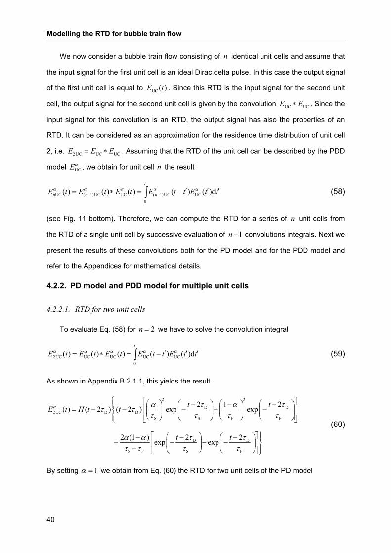
Modelling the RTD for bubble train flow
40
We now consider a bubble train flow consisting of n identical unit cells and assume that
the input signal for the first unit cell is an ideal Dirac delta pulse. In this case the output signal
of the first unit cell is equal to UC ( )E t . Since this RTD is the input signal for the second unit
cell, the output signal for the second unit cell is given by the convolution UC UCE E∗ . Since the
input signal for this convolution is an RTD, the output signal has also the properties of an
RTD. It can be considered as an approximation for the residence time distribution of unit cell
2, i.e. 2UC UC UCE E E= ∗ . Assuming that the RTD of the unit cell can be described by the PDD
model UCEα , we obtain for unit cell n the result
UC ( 1)UC UC ( 1)UC UC0
( ) ( ) ( ) ( ) ( )dt
n n nE t E t E t E t t E t tα α α α α− − ′ ′ ′= ∗ = −∫ (58)
(see Fig. 11 bottom). Therefore, we can compute the RTD for a series of n unit cells from
the RTD of a single unit cell by successive evaluation of 1n − convolutions integrals. Next we
present the results of these convolutions both for the PD model and for the PDD model and
refer to the Appendices for mathematical details.
4.2.2. PD model and PDD model for multiple unit cells
4.2.2.1. RTD for two unit cells
To evaluate Eq. (58) for 2n = we have to solve the convolution integral
2UC UC UC UC UC0
( ) ( ) ( ) ( ) ( )dt
E t E t E t E t t E t tα α α α α′ ′ ′= ∗ = −∫ (59)
As shown in Appendix B.2.1.1, this yields the result
2 2
D D2UC D D
S S F F
D D
S F S F
2 21( ) ( 2 ) ( 2 ) exp exp
2 22 (1 ) exp exp
t tE t H t t
t t
α τ τα ατ ττ τ τ τ
τ τα ατ τ τ τ
⎧ ⎡ ⎤⎛ ⎞ ⎛ ⎞ ⎛ ⎞ ⎛ ⎞− −−⎪ ⎢ ⎥= − − − + −⎨ ⎜ ⎟ ⎜ ⎟ ⎜ ⎟ ⎜ ⎟⎢ ⎥⎝ ⎠ ⎝ ⎠⎝ ⎠ ⎝ ⎠⎪ ⎣ ⎦⎩
⎫⎡ ⎤⎛ ⎞ ⎛ ⎞− −− ⎪+ − − − ⎬⎢ ⎥⎜ ⎟ ⎜ ⎟− ⎝ ⎠⎝ ⎠ ⎪⎣ ⎦⎭
(60)
By setting 1α = we obtain from Eq. (60) the RTD for two unit cells of the PD model

Modelling the RTD for bubble train flow
41
D D2UC D2
S S
2 2( ) exp ( 2 )t tE t H tτ τ ττ τ
⎛ ⎞− −= − −⎜ ⎟
⎝ ⎠ (61)
(see also Appendix A.2.1.1).
As shown in Appendix B.2.1.2, the mean residence time for two unit cells is
2UC 2UC 2UC D S F UC0
( )d 2 (1 ) 2t tE t tα α α ατ τ ατ α τ τ∞
⎡ ⎤≡ = = + + − =⎣ ⎦∫ (62)
For 1α = we obtain the result (see also Appendix A.2.1.2)
2UC D S2( )τ τ τ= + (63)
The non-dimensional time for two unit cells is defined as
D2UC
UC
22
tαα
τθτ−
≡ (64)
Then, the RTD for two unit cells can be written in the non-dimensional form
( )
2UC UC 2UC
2 2
UC UC UC UC2UC 2UC 2UC
S S F F
UC UC UC2UC 2UC UC
S F S F
( ) 2 ( )
2 2 2 2exp 1 exp
4 2 2(1 ) exp exp (2
E E t
H
α α αθ
α α α αα α α
α α αα α α
θ τ
τ τ τ τθ α θ α θτ τ τ τ
τ τ τα α θ θ ττ τ τ τ
=
⎧ ⎡ ⎤⎛ ⎞ ⎛ ⎞ ⎛ ⎞ ⎛ ⎞⎪ ⎢ ⎥= − + − −⎨ ⎜ ⎟ ⎜ ⎟ ⎜ ⎟ ⎜ ⎟⎢ ⎥⎝ ⎠ ⎝ ⎠⎝ ⎠ ⎝ ⎠⎪ ⎣ ⎦⎩
⎫⎡ ⎤⎛ ⎞ ⎛ ⎞ ⎪+ − − − − ⎬⎢ ⎥⎜ ⎟ ⎜ ⎟− ⎝ ⎠⎝ ⎠ ⎪⎣ ⎦⎭
,
2UC )αθ
(65)
For 1α = we obtain
2
UC UC,2UC 2UC 2UC UC 2UC
S S
2 2( ) exp (2 )E Hα α
αθ
τ τθ θ θ τ θτ τ
⎛ ⎞ ⎛ ⎞= −⎜ ⎟ ⎜ ⎟
⎝ ⎠ ⎝ ⎠ (66)
We now compare the RTD for two unit cells obtained by this convolution procedure with
the numerically evaluated RTD curves. Fig. 12 a) and b) show the results for cases A2 and
B2 both for the PD model and the PDD model (for two different values of β ). Comparing the
model RTDs for two unit cells in Fig. 12 a) and b) with those in Fig. 10 a) and b) for one unit
cell shows one apparent difference. Namely, for one unit cell the RTD is zero for Dt τ< ,
jumps to it maximum value at Dt τ= and decreased monotonically to zero for values Dt τ> .

Modelling the RTD for bubble train flow
42
Instead, for two unit cells the model RTD is zero for Dt τ≤ , increases till a maximum value is
obtained and finally decreases toward zero. The maximum value of the RTD is always higher
for the PD model than for the PDD model, both for the single unit cell and for two unit cells.
Fig. 12 a) and b) show that for the PDD model the maximum value of the RTD is very
sensitive to the value of β . We recall, as noted before, that the maximum value of the
numerically evaluated RTD is sensitive to the value of classtΔ . In all cases, the RTD curve of
the PDD model intersects that of the PD model, giving lower values of the RTD at low values
of t and higher values of the RTD at large values of t as compared to the PD model. Due to
this behaviour the PDD model provides a better fit to the long tails of the numerical RTD for
two unit cells, see Fig. 12 a) and b). Interestingly, in the numerical RTD there appears a
second peak at ref/ 4.3t t ≈ for case A2 and for ref/ 6t t ≈ for case B2. The inset graphics in
Fig. 12 a) and b) show, that at high values of t the slope of the numerical RTD is well
approximated by the PDD model with a value of 1β = for case A2, and 0.97β = for case
B2.

Modelling the RTD for bubble train flow
43
Fig. 12: Comparison of numerically evaluated RTD curves for case A2 (a) and B2 (b) with
the PD model and the PDD model. The dashed vertical lines correspond to the delay time
for each case.

Modelling the RTD for bubble train flow
44
4.2.2.2. RTD for three unit cells
For the PD model, the output signal for three unit cells is given by
3UC 2UC UC 2UC UC0
( ) ( ) ( ) ( ) ( )dt
E t E t E t E t t E t t′ ′ ′= ∗ = −∫ (67)
The evaluation of this convolution integral yields the result
2D D
3UC D3S S
( 3 ) 3( ) exp ( 3 )2
t tE t H tτ τ ττ τ
⎛ ⎞− −= − −⎜ ⎟
⎝ ⎠, (68)
see Appendix A.2.2.1. The mean residence time is
3UC 3UC 3UC S D UC0
( )d 3( ) 3t tE t tτ τ τ τ∞
≡ = = + =∫ , (69)
see Appendix A.2.2.2. The non-dimensional time for three unit cells is defined as
D3UC
UC
33
t τθτ−
≡ (70)
so that Eq. (68) can be written in the following non-dimensional form
323UC UC UC
,3UC UC 3UC 3UC UC 3UCS S
3 ( ) 3 exp 3 (3 )2
E E t Hθθ τ ττ θ τ θ
τ τ⎛ ⎞ ⎛ ⎞
≡ = −⎜ ⎟ ⎜ ⎟⎝ ⎠ ⎝ ⎠
(71)
For the PDD model, the RTD 3UC ( )E tα for three unit cells becomes very complicated so
that the convolution integral is evaluated by Laplace transformation. The result can be found
at the end of Appendix C and is not repeated here.
In Fig. 13 we compare the RTD of the PD and PDD model for three unit cells with the
numerically evaluated RTD curves for case A1 and B1. Similar as for two unit cells, there is a
notable difference between the heights of the peaks. Higher residence times are not
accurately represented by the PD model but are reasonably represented by the PDD model.
However both for the PD model and the PDD model, the location of the maximum of the RTD
is shifted to larger times as compared to the numerically evaluated RTD. It is expected that
this discrepancy will even increase for larger numbers of unit cells in series.
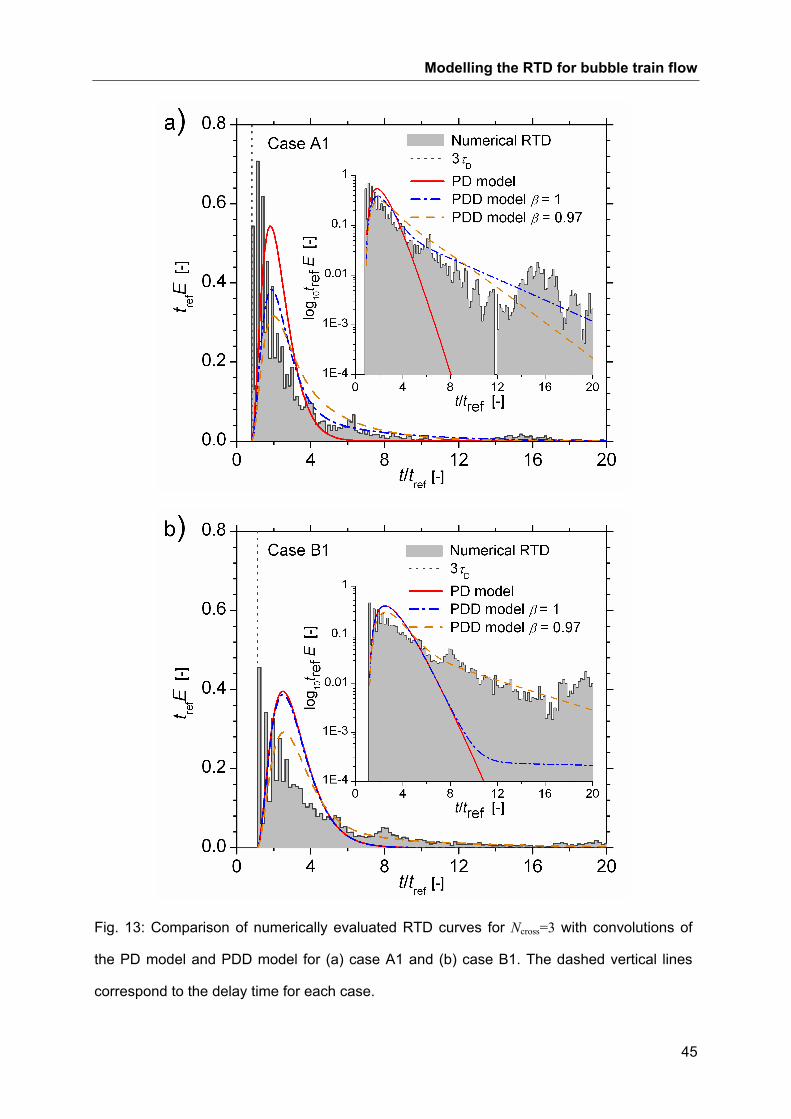
Modelling the RTD for bubble train flow
45
Fig. 13: Comparison of numerically evaluated RTD curves for Ncross=3 with convolutions of
the PD model and PDD model for (a) case A1 and (b) case B1. The dashed vertical lines
correspond to the delay time for each case.

Modelling the RTD for bubble train flow
46
4.2.2.3. General RTD model
The RTD of the PD model for four unit cells is
3D D
4UC D4S S
( 4 ) 4( ) exp ( 4 )6
t tE t H tτ τ ττ τ
⎛ ⎞− −= − −⎜ ⎟
⎝ ⎠ (72)
see Appendix A.2.3. The mean residence time is
4UC 4UC 4UC S D UC0
( )d 4( ) 4t tE t tτ τ τ τ∞
≡ = = + =∫ (73)
As shown in Appendix C, the PD model for n identical unit cells in series is
1D D
UC DS S
( )( ) exp ( )( 1)
n
n n
t n t nE t H t nn
τ τ ττ τ
− ⎛ ⎞− −= − −⎜ ⎟− ! ⎝ ⎠
(74)
The mean residence time of this RTD is
( )UC S Dn nτ τ τ= + (75)
With the non-dimensional time defined in Eq. (25), the RTD of the PD model for n unit cells
can be written in the general form
1UC UC UC
UC UC UC UC UC UCS S
( ) ( ) exp ( )( 1)
nnn
n n n nE n E t n n H nnθθ τ τθ τ θ τ θ
τ τ
− ⎛ ⎞ ⎛ ⎞= = −⎜ ⎟ ⎜ ⎟− !⎝ ⎠ ⎝ ⎠
, (76)
This RTD for a cascade of n identical unit cells is equivalent to the RTD of a cascade of n
identical CSTRs in series given in Eq. (20). For D 0τ = we have UC Sτ τ= and Eq. (76) be-
comes identical to Eq. (20).
For the PDD model, the RTD becomes increasingly complex for an increasing number of
unit cells, see Appendix C. Therefore, this model is hardly useful for large values of n . Thus,
simpler models for a large number of unit cells shall be developed in future, which accurately
represent the tail of the RTD, and, even more important, correctly predict both (i) the sharp
increase of the RTD for values of t slightly higher than the delay time and (ii) the location of
the maximum value of the RTD.
Conclusions
47
5. Conclusions
In this report, we used results from direct numerical simulations of a bubble train flow in a
square vertical mini-channel to develop an analytical model for the prediction of the liquid
phase residence time distribution from given integral flow parameters. For this purpose, the
unit cell RTD model of Wörner, Ghidersa, Onea (2007) (the WGO model), which was
developed for co-current upward flow and can be represented by a compartment model
consisting of a plug flow reactor (PFR) and a continuous-stirred-tank reactor (CSTR) in
series, was improved with respect to two aspects. First, in the peak-decay (PD) model the
delay time of the RTD (which corresponds to the residence time of the PFR) is consistently
formulated to be valid in both co-current upward and downward bubble train flow. Second, to
account better for the long tails of the RTD, the compartment model was further refined and
consists in the peak-decay-decay (PDD) model of a PFR in series with two CSTRs in
parallel. The two CSTRs represent the liquid slug and liquid film / corner flow region,
respectively. Both CSTRs have a different mean residence time. The resulting RTD consists
of the superposition of two decaying exponential terms showing different slopes. It is shown
that the PDD model accurately represents the numerically evaluated unit cell RTD for
different flow conditions.
In practical applications, not the RTD of the unit cell but that of a bubble train flow
consisting of a finite number of unit cells is of interest. In this report, the RTD for n unit cells
in series is determined from the unit cell RTD by a ( 1)n − -fold convolution procedure. For the
PD model these convolutions can be evaluated analytically and yield a rather simple and
general expression. For the PDD model, however, the analytical evaluation of these
convolution integrals is becoming increasingly complex and is - without further
approximations – of limited practical use for 4.n > The comparison of the convolution based
PD and PDD models for 2n = and 3n = with the numerically evaluated RTD has shown,
however, that the agreement is not satisfactory. In particular, the models overestimate the
residence time for which the RTD has its maximum value. It appears that this discrepancy
Conclusions
48
even increases with increasing value of n . Thus we conclude that in future the RTD model
for multiple unit cells should be further improved.
Concerning the unit cell RTD, further issues that should be investigated in future are the
consideration of numerical simulations with longer liquid slugs and the reason for the
appearance of a second peak in the numerically evaluated unit cell RTD at the residence
time where - in a semi-logarithmic representation - the RTD changes its slope. While
measurements of the unit cell RTD are not available in literature, there exist experimental
data for a single channel that should be used for validation of the RTD model for multiple unit
cells.
Acknowledgement
The authors gratefully acknowledge the supports of EU Erasmus program and of Institute
of Science and Technology at Sakarya University. We also acknowledge the support of Dr.
Hakan S. Soyhan who was the main supervisor of S.E. at Sakarya University, Turkey, during
this research project for master thesis.

References
49
References
Abiev, R. Sh., 2008. Simulation of the slug flow of a gas-liquid system in capillaries. Theor.
Found. Chem. Eng. 42, 105−127.
Angeli, P., Gavriilidis, A., 2008. Hydrodynamics of Taylor flow in small channels: a review.
Proc. IMechE Part C: J. Mech. Eng. Sci. 222, 737−751.
Bakker, J.J.W., Kreutzer, M., de Lathouder, K., Kapteijn, F., Moulijn, J.A., Wallin, S.A., 2005.
Hydrodynamic properties of a novel ‘open wall’ monolith reactor. Catalysis Today 105,
385−390.
Bauer, T., Guettel, R., Roy, S., Schubert, M., Al-Dahhan, M., Lange, R., 2005. Modelling and
simulation of the monolithic reactor for gas-liquid-solid reactions. Chem. Eng. Res. Design
83, 811−819.
Bradford, M.C.J., Tem M., Pollack, A., 2005. Monolith loop catalytic membrane reactor for
Fischer-Tropsch synthesis. Applied Catalysis A: General 283, 39−46.
Burns, J.R., Ramshaw, C., 2001. The intensification of rapid reactions in multiphase systems
using slug flow in capillaries. Lab Chip 1, 10-15.
De Deugd, R.M., Chougule, R.B., Kreutzer, M.T., Meeuse, F.M., Grievink, J., Kapteijn, F.,
Moulijn, J.A., 2003. Is a monolithic loop reactor a viable option for Fischer-Tropsch
synthesis? Chem. Eng. Sci. 58, 583−591.
Edvinsson Albers, R., Nyström, M., Siverström, M., Sellin, A., Dellve, A.-C., Andersson, U.,
Herrmann, W., Berglin, Th., 2001. Development of a monolith-based process for H2O2
production: from idea to large-scale implementation. Catalysis Today 69, 247−252.
Fogler, H.S., 1986. Elements of Chemical Reaction Engineering. Prentice Hall.
Fries, D.M., von Rohr, P.R., 2009. Impact of inlet design on mass transfer in gas-liquid
rectangular microchannels. Microfluid Nanofluid 6, 27−35.

References
50
Ghidersa, B., Wörner, M., Cacuci, D.G., 2004. Exploring the flow of immiscible fluids in a
square vertical mini-channel by direct numerical simulation. Chem. Eng. J. 101, 285−294.
Günther, A., Khan, S.A., Thalmann, M., Trachsel, F., Jensen, K.F., 2004. Transport and
reaction in microscale segmented gas-liquid flow. Lab Chip 4, 278−286.
Güttel R., Kunz, U., Turek, T., 2008. Reactors for Fischer-Tropsch synthesis. Chem. Eng.
Technol. 31, 746−754.
Haverkamp, V., Hessel, V., Löwe, H., Menges, G., Warnier, M.J.F., Rebrov, E.V., de Croon,
M.H.J.M., Schouten, J.C., Liauw, M., 2006. Hydrodynamics and mixer-induced bubble forma-
tion in microbubble columns with single and multiple channels. Chem. Eng. Technol. 29,
1015−1026.
Heibel, A.K., Lebens, P.J.M., Middelhoff, J.W., Kapteijn, F., Moulijn, J., 2005. Liquid resi-
dence time distribution in the film flow monolith reactor. AICHE J. 51, 122−133.
Jähnisch, K., Baerns, M., Hessel, V., Ehrfeld, W., Haverkamp, V., Löwe, H., Wille, Ch.,
Guber, A., 2000. Direct fluorination of toluene using elemental fluorine in gas/liquid micro-
reactors. J. Fluor. Chem. 105, 117−128.
Kreutzer, M.T., Bakker, J.J.W., Kapteijn, F., Moulijn, J.A., Verheijen, P.J.T., 2005a. Scaling-
up multiphase monolith reactors: linking residence time distribution and feed maldistribution.
Ind. Eng. Chem. Res. 44, 4898−4913.
Kreutzer, M.T., Kapteijn, F., Moulijn, J.A., Heiszwolf, J.J., 2005b. Multiphase monolith reac-
tors: chemical reaction engineering of segmented flow in microchannels. Chem. Eng. Sci. 60,
5895−5916.
Kulkarni, R., Natividad, R., Wood, J., Stitt, E.H., Winterbottom, J.M., 2005. A comparative
study of residence time distribution and selectivity in a monolith CDC reactor and a trickle
bed reactor. Catalysis Today 105, 455−463.
Levenspiel, O., 1999. Chemical Reaction Engineering, third ed. Wiley, New York.

References
51
Liu, W., Hu, J., Wang, Y., 2009. Fischer-Tropsch synthesis on ceramic monolith-structured
catalysts. Catalysis Today 140, 142−148.
Lohse , S., Kohnen, B.T., Janasek, D., Dittrich, P.S., Franzke, J., Agar, D.W., 2008. A novel
method for determining the residence time distribution in intricately structured microreactors.
Lab Chip 8, 431−438.
Mantle, M.D., Sederman, A.J., Gladden, L.F., Raymahasay, S., Winterbottom, J.M., Stitt,
E.H., 2002. Dynamic MRI visualization of two-phase flow in a ceramic monolith. AIChE J. 48,
909−912.
Martin, A.D., 2000. Interpretation of residence time distribution data. Chem. Eng. Sci. 55,
5907−5917.
Mc Collum, P.A., Brown, B.F., 1965. Laplace Transform Tables and Theorems. Holt,
Rinehart and Winston, New York.
Nauman, E.B., 2008. Residence time theory. Ind. Eng. Chem. Res. 47, 3752−3766.
Özkan, F., Wörner, M., Wenka, A., Soyhan, H.S., 2007. Critical evaluation of CFD codes for
interfacial simulation of bubble-train flow in a narrow channel. Int. J. Numer. Meth. Fluids 55,
537–564.
Öztaskin, M.C., Wörner, M., Soyhan, H.S., 2009. Numerical investigation of the stability of
bubble train flow in a square mini-channel. Phys. Fluids 21, 042108-1 − 042108-17.
Patrick, R.H. Jr., Klindera, T., Crynes L.L., Cerro, R.L., Abraham, M.A., 1995. Residence
time distribution in three-phase monolith reactor. AIChE J. 41, 649−657.
Pedersen, H., Horvath, C., 1981. Axial dispersion in a segmented gas-liquid flow. Ind. & Eng.
Chem. Fund. 20, 181−186.
Roberts, G.E., Kaufman, H., 1966. Table of Laplace Transforms. W.B. Saunders Company,
Philadelphia and New York.
Roy, S., Bauer, T., Al-Dahhan, M., Lehner, P., Turek, S., 2004. Monoliths as multiphase re-
actors: a review. AIChE J. 50, 2918−2938.

References
52
Sabisch, W., 2000. Dreidimensionale numerische Simulation der Dynamik von aufsteigenden
Einzelblasen und Blasenschwärmen mit einer Volume-of-Fluid Methode. Forschungszentrum
Karlsruhe, Wissenschaftliche Berichte FZKA 6478, Juni 2000.
Sabisch, W., Wörner, M., Grötzbach, G., Cacuci, D.G., 2001. 3D volume-of-fluid simulation of
a wobbling bubble in a gas–liquid system of low Morton number. In: Proc. 4th Int. Conf. Mul-
tiphase Flow, New Orleans, USA, May 27–June 1, 2001.
Salman, W., Gavriilidis, A., Angeli, P., 2004. A model for predicting axial mixing during gas-
liquid Taylor flow in microchannels at low Bodenstein numbers. Chem. Eng. J. 101, 391−396.
Salman, W., Angeli, P., Gavriilidis, A., 2005. Sample pulse broadening in Taylor flow micro-
channels for screening applications. Chem. Eng. Technol. 28, 509−514.
Salman, W., Gavriilidis, A., Angeli, P., 2007. Axial mass transfer in Taylor flow through circu-
lar microchannels. AIChE J. 53, 1413−1428.
Shah, R.K., London, A.L., 1978. Laminar flow forced convection in ducts. Academic Press,
pg. 198.
Sun, J., Ju, J., Ji, L., Zhang, L., Xu, N., 2008. Synthesis of biodiesel in capillary microreac-
tors. Ind. Eng. Chem. Res. 47, 1398−1403.
Thulasidas, T.C., Abraham, M.A., Cerro, R.L., 1997. Flow patterns in liquid slugs during
bubble-train flow inside capillaries. Chem. Eng. Sci. 52, 2947−2962.
Thulasidas, T.C., Abraham, M.A., Cerro, R.L., 1999. Dispersion during bubble-train flow in
capillaries. Chem. Eng. Sci. 54, 61−76.
Trachsel, F., Günther, A., Khan, S., Jensen, K.F., 2005. Measurement of residence time dis-
tribution in microfluidic systems. Chem. Eng. Sci. 60, 5729−5737.
Tsoligkas, A.N., Simmons, M.J.H., Wood, J., 2007. Influence of orientation upon the hydro-
dynamics of gas-liquid flow for square channels in monolith supports. Chem. Eng. Sci. 62,
4365−4378.

References
53
Wörner, M., Ghidersa, B., Onea, A., 2007. A model for the residence time distribution of
bubbe-train-flow in a square mini-channel based on direct numerical simulation results. Int. J.
Heat Fluid Flow, 28, 83−94.
Yawalkar, A.A., Sood, R., Kreutzer, M.T., Kapteijn, F., Moulijn, J.A., 2005. Axial mixing in
monolith reactors: effect of channel size. Ind. Eng. Chem. Res. 44, 2046−2057.

Appendix
54
Appendix A. Integral evaluations for PD model To evaluate the various integrals in this Appendix and in Appendix B we will - without fur-
ther notice - take advantage of the identity
1 /
0
d ( 1)!∞
− − = −∫ n z a nz e z n a
A.1. Evaluations for one unit cell A.1.1. Integral of RTD
The integral of the PD model for one unit cell is
D S D S D S S
D D
D S S D S S D S D S
D D
( )/ ( )/ / /1 1 1UC D S S S
0 0
/ / / / / /1 0S S
( )d ( ) e d e d e e d
e e e e e 0 e e 1
t t t
t t
E t t H t t t tτ τ τ τ τ τ τ
τ τ
τ τ τ τ τ τ τ τ τ τ
τ τ
τ τ τ τ
τ τ
∞ ∞ ∞ ∞− − − − −− − −
∞ ∞− − −−
= − = =
⎡ ⎤ ⎡ ⎤ ⎡ ⎤= − = − = − − = =⎣ ⎦ ⎣ ⎦ ⎣ ⎦
∫ ∫ ∫ ∫
A.1.2. Mean residence time
The mean residence time of the PD model for one unit cell is
D S D S D S S
D D
D S S D S S D S S S
D D D
( )/ ( )/ / /1 1 1UC UC D S S S
0 0
/ / / / / / /1 2 1 1 1S S S S S s S
S
( )d ( ) e d e d e e d
e ( 1)e e ( 1)e e e e
t t t
t t t t
tE t t tH t t t t t t
t t t
τ τ τ τ τ τ τ
τ τ
τ τ τ τ τ τ τ τ τ τ
τ τ τ
τ τ τ τ τ
τ τ τ τ τ τ τ
τ
∞ ∞ ∞ ∞− − − − −− − −
∞ ∞ ∞− − − −− − − −
= = − = =
⎡ ⎤ ⎡ ⎤ ⎡ ⎤= − − = − + = − +⎣ ⎦ ⎣ ⎦ ⎣ ⎦
= −
∫ ∫ ∫ ∫
D S S D S D S D S D S
S
D S D s D S D S
S
/ / / / / /1 1 1S D S S D S/
S
/ / / /1 1S D s S D S D S/
e lim e 0 ( e ) e e lim e ( 1)e
lim1 1e e ( 1) e e ( 1)lim e
ttt t
tz
t
ttτ τ τ τ τ τ τ τ τ τ ττ
τ τ τ τ τ τ τ ττ
τ τ τ τ τ ττ
τ τ τ τ τ τ τ τ
− − − −− − −
→∞ →∞
− −− −→∞
→∞
⎡ ⎤⎡ ⎤+ − − = − − +⎢ ⎥⎣ ⎦ ⎣ ⎦
⎡ ⎤ ⎡ ⎤⎢ ⎥= − − + = − − + = +⎢ ⎥∞⎢ ⎥ ⎣ ⎦⎣ ⎦
A.1.3. Variance
The variance of the PD model for one unit cell is
( ) D S2 ( )/2 2 1
UC UC UC D S D S0 0
σ ( ) ( )d ( ) ( ) e dtt t E t t t H t tτ ττ τ τ τ∞ ∞
− −−= − = − + −∫ ∫
We introduce the substitution Dz t τ≡ − so that d dz t= . This gives

Appendix
55
( )
( )
( )
D S S
D
S S S S
S
2 ( )/ /2 1 2 1UC D S D S S S
0
/ / / /1 2 2 1 2 2s S S S S S
0 0
/ /1 2 2 3 2 1S S S S S S S0
σ ( ) ( ) e d ( ) ( ) e d
( 2 )e d e 2 e e d
2 2 e 2 ( 1)e
τ τ τ
τ
τ τ τ τ
τ τ
τ τ τ τ τ τ
τ τ τ τ τ τ
τ τ τ τ τ τ τ
∞ ∞− − −− −
−
∞ ∞− − − −− −
∞− −− −
= − + − = −
⎡ ⎤= − + = − +⎢ ⎥
⎣ ⎦
⎡ ⎤= − − − − − −⎣ ⎦
∫ ∫
∫ ∫
t z
z z z z
z z
t H t t z H z z
z z z z z z
z z z{ }( ) [ ]{ }
S S
S S S
S S S
/2S S0 0
/ / /1 2 2 3 3 1 3S S S S S S S
2S1 3 3S
S S S/ / /1 1S S S
e
lim( e ) lim(2 e ) 2 2 lim e 1 0 1
lim 222 lim 2 lim 1e lim e e
τ
τ τ τ
τ τ τ
τ τ
τ τ τ τ τ τ τ
τττ τ ττ τ τ
∞ ∞−
− − −− −
→∞ →∞ →∞
− →∞− −→∞ →∞
→∞
⎡ ⎤ ⎡ ⎤+ −⎣ ⎦ ⎣ ⎦
⎡ ⎤ ⎡ ⎤= − − + + − − −⎢ ⎥ ⎣ ⎦⎣ ⎦
⎛ ⎞⎜ ⎟= − − + −⎜ ⎟⎝ ⎠
z
z z z
z z z
zz z zz z
z
z z z
z z
( ) ( )
S S
3S
2S1 3 3 3S
S S S S/ /2S
1 3 3 3 1 3 3 3 2SS S S S S S S S S
lim 2 lim122 2 1lim e lim e
22 2 0 1 2 2
τ τ
τ
τ ττ τ τ ττ
ττ τ τ τ τ τ τ τ τ
− →∞ →∞−
→∞ →∞
− −
⎡ ⎤⎛ ⎞⎢ ⎥+⎜ ⎟⎢ ⎥⎝ ⎠⎣ ⎦
⎡ ⎤⎛ ⎞ ⎛ ⎞⎢ ⎥⎜ ⎟ ⎜ ⎟= − − + − +⎜ ⎟ ⎜ ⎟∞⎢ ⎥⎝ ⎠ ⎝ ⎠⎣ ⎦
⎡ ⎤⎛ ⎞= − + − + = − + =⎜ ⎟⎢ ⎥∞⎝ ⎠⎣ ⎦
z zz z
z z
A.2. Evaluations for multiple unit cells A.2.1. Evaluations for two unit cells
A.2.1.1. Convolution integral for two unit cells
The convolution integral of the PD model for two unit cells is
2UC UC UC UC UC0
( ) ( ) ( ) ( ) ( )dt
E t E t E t E t t E t t′ ′ ′= ∗ = −∫
This integral is given by
D S D S
D S D S
( )/ ( )/1 12UC D S D S
0
( 2 )/ ( 2 )/2 2D D S S D D
0 0
( ) ( ) e ( ) e d
( ) ( ) e d e ( ) ( )d
tt t t
t tt t
E t H t t H t t
H t t H t t H t t H t t
τ τ τ τ
τ τ τ τ
τ τ τ τ
τ τ τ τ τ τ
′ ′− − − − −− −
− − − −− −
′ ′ ′= − − −
′ ′ ′ ′ ′ ′= − − − = − − −
∫
∫ ∫
To evaluate the integral with the two Heaviside step functions we introduce the substitution
Du t τ′≡ − so that d du t′= . This gives
D D
D
D D D D0 0
( ) ( )d ( 2 ) ( )d ( 2 )dt tt
I H t t H t t H t u H u u H t u uτ τ
τ
τ τ τ τ− −
−
′ ′ ′≡ − − − = − − = − −∫ ∫ ∫

Appendix
56
Next we introduce a second substitution D2w u t τ≡ − + − so that d dw u= − . This gives
[ ]
D D D D
D D
DD
2 2
D0 2 0
22
D D D D00
( 2 )d ( )d ( )d ( )d
( 2 ) d ( 2 ) ( 2 ) ( 2 )
t t t
t
tt
I H t u u H w w H w w H w w
H t w H t w t H t
τ τ τ τ
τ τ
ττ
τ
τ τ τ τ
− − − −
− −
−−
= − − = − = =
= − = − = − −
∫ ∫ ∫ ∫
∫
Thus, we obtain
D( 2 )/22UC D D S( ) ( 2 )( 2 ) e StE t H t t τ ττ τ τ − −−= − −
The integral of 2UC ( )E t is given by
D S( 2 )/22UC D D S
0 0
( )d ( 2 )( 2 ) e dtE t t H t t tτ ττ τ τ∞ ∞
− −−= − −∫ ∫
We introduce the substitution D2z t τ≡ − and obtain
D S S
D
S S S S S
S
( 2 )/ /2 22UC D D S S
0 0 2
/ / / / /2 2 2 1 1 1S S S S S S0 0 0
0
/1S
( )d ( 2 )( 2 ) e d ( ) e d
e d ( 1)e ( 1)e e e
lim e 0 0 1 1 lim
t z
z z z z z
z
z
E t t H t t t H z z z
z z z z z
z
τ τ τ
τ
τ τ τ τ τ
τ
τ τ τ τ
τ τ τ τ τ τ
τ
∞ ∞ ∞− − −− −
−
∞∞ ∞ ∞− − − − −− − − − −
−−
→∞
= − − =
⎡ ⎤ ⎡ ⎤ ⎡ ⎤= = − − = − + = − +⎣ ⎦ ⎣ ⎦ ⎣ ⎦
= − − + + = −
∫ ∫ ∫
∫
S S/ /S
lim1 11 1 1e lim e
zz zz
z
zτ ττ
→∞
→∞→∞
= − = − =∞
A.2.1.2. Mean residence time for two unit cells
The mean residence time for a length of two unit cells is
D S( 2 )/22UC 2UC D D S
0 0
( )d ( 2 )( 2 ) e dtt tE t t tH t t tτ ττ τ τ∞ ∞
− −−= = − −∫ ∫
We introduce the substitution D2z t τ≡ − and obtain
D S S
D
S S S
( 2 )/ /2 22UC 2UC D D S D S
0 0 2
/ / /2 2 2D S S D
0 0
( )d ( 2 )( 2 ) e d ( 2 ) ( ) e d
( 2 ) e d e 2 e d
t z
z z z
t tE t t tH t t t z H z z z
z z z z z z
τ τ τ
τ
τ τ τ
τ τ τ τ τ
τ τ τ τ
∞ ∞ ∞− − −− −
−
∞ ∞− − −− −
= = − − = +
⎡ ⎤= + = +⎣ ⎦
∫ ∫ ∫
∫ ∫

Appendix
57
and thus
( ){ }s S/ /2 2 2 3 2 12UC S S S S D S S 00
2 3 2S S D S S D
2 2 e 2 ( 1)e
2 2 2( )
z zt z z zτ ττ τ τ τ τ τ τ
τ τ τ τ τ τ
∞ ∞− −− −
−
⎡ ⎤ ⎡ ⎤= − − − + − −⎣ ⎦⎣ ⎦
⎡ ⎤= + = +⎣ ⎦
A.2.2. Evaluations for three unit cells
A.2.2.1. Convolution integral for three unit cells
The convolution integral of the PD model for three unit cells is
3UC 2UC UC 2UC UC0
( ) ( ) ( ) ( ) ( )dt
E t E t E t E t t E t t′ ′ ′= ∗ = −∫
This integral is given by
D S D S
D S
D S
( 2 )/ ( )/2 13UC D D S D S
0
( 3 )/3D D D S
0
( 3 )/3S D D D
0
( ) ( 2 )( 2 ) e ( ) e d
( 2 ) ( )( 2 ) e d
e ( 2 ) ( 2 ) ( )d
tt t t
tt
tt
E t H t t t t H t t
H t t H t t t t
t t H t t H t t
τ τ τ τ
τ τ
τ τ
τ τ τ τ τ
τ τ τ τ
τ τ τ τ
′ ′− − − − −− −
− −−
− −−
′ ′ ′ ′= − − − − −
′ ′ ′ ′= − − − − −
′ ′ ′ ′= − − − − −
∫
∫
∫
To evaluate the integral with the two Heaviside step functions we introduce the substitution
Du t τ′≡ − so that d du t′= . This gives
D
D
D
D D D D D0
D D0
( 2 ) ( 2 ) ( )d ( 3 ) ( 3 ) ( )d
( 3 ) ( 3 )d
tt
t
I t t H t t H t t t u H t u H u u
t u H t u u
τ
τ
τ
τ τ τ τ τ
τ τ
−
−
−
′ ′ ′ ′≡ − − − − − = − − − −
= − − − −
∫ ∫
∫
Next we introduce a second substitution D3w u t τ≡ − + − so that d dw u= − . This gives
D D D D
D D
DD
2 3 3
D D0 3 2 0
33 22
D D D D0 0
( 3 ) ( 3 )d ( )d ( )d ( )d
1( 3 ) d ( 3 ) ( 3 ) ( 3 )2 2
t t t
t
tt
I t u H t u u wH w w wH w w wH w w
wH t w w H t t H t
τ τ τ τ
τ τ
ττ
τ τ
τ τ τ τ
− − − −
− −
−−
= − − − − = − = =
⎡ ⎤= − = − = − −⎢ ⎥
⎣ ⎦
∫ ∫ ∫ ∫
∫
Thus, we obtain

Appendix
58
D S( 3 )/2 33UC D D S
1( ) ( 3 ) ( 3 ) e2
tE t H t t τ ττ τ τ − −−= − −
The integral of 3UC ( )E t is given by
D S( 3 )/2 33UC D D S
0 0
1( )d ( 3 )( 3 ) e d2
tE t t H t t tτ ττ τ τ∞ ∞
− −−= − −∫ ∫
We introduce the substitution D3z t τ≡ − and obtain
( )
D S S
D
S S
S S S
( 3 )/ /2 3 2 33UC D D S S
0 0 3
/ /3 2 3 2 2 3S S S S S 0
0
/ / /3 2 2 3S S S S 0
3 2S S
1 1( )d ( 3 )( 3 ) e d ( ) e d2 2
1 1e d 2 2 e2 2
1 e 2 e 2 e2
1 lim(2
τ τ τ
τ
τ τ
τ τ τ
τ τ τ τ
τ τ τ τ τ
τ τ τ τ
τ τ
∞ ∞ ∞− − −− −
−
∞ ∞− −− −
∞− − −−
−
→∞
= − − =
⎡ ⎤= = − − −⎣ ⎦
⎡ ⎤= − − −⎣ ⎦
= −
∫ ∫ ∫
∫
t z
z z
z z z
z
E t t H t t t H z z z
z z z z
z z
z( )S S
S S S S
S
/ /2 3S S
22 2S3 3 3 3S S S
S S S S/ / / /1 1s S
2S3 3 S
S S /2s
e ) lim(2 e ) 0 0 0 2
lim 22 21 12 lim lim 2 lim2 e e 2 e lim e
lim 2 21 22 lim e
τ τ
τ τ τ τ
τ
τ τ
ττ τ ττ τ τ ττ τ
τ ττ ττ
− −
→∞
− − →∞− −→∞ →∞ →∞
→∞
− →∞−
→∞
⎡ ⎤− − + + +⎢ ⎥⎣ ⎦
⎛ ⎞⎛ ⎞ ⎜ ⎟= − − = − −⎜ ⎟ ⎜ ⎟⎝ ⎠ ⎝ ⎠
= − −
z z
z
zz z z zz z z
z
zz
z
z
z z z
3 3 SS S
21 2 12
ττ τ−⎛ ⎞ ⎛ ⎞⎜ ⎟ = − =⎜ ⎟⎜ ⎟∞ ∞⎝ ⎠⎝ ⎠
A.2.2.2. Mean residence time for three unit cells
The mean residence time for three unit cells is
D S( 3 )/2 33UC 3UC D D S
0 0
1( )d ( 3 )( 3 ) e d2
tt tE t t t H t t tτ ττ τ τ∞ ∞
− −−= = − −∫ ∫
We introduce the substitution D3z t τ≡ − and obtain
( )
( )
D S S
D
S S S
( 3 )/ /2 3 2 33UC 3UC D D S D S
0 0 3
/ / /3 2 3 3 2S D S D
0 0
1 1( )d ( 3 )( 3 ) e d 3 ( ) e d2 2
1 13 e d e 3 e d2 2
t z
z z z
t tE t t t H t t t z H z z z
z z z z z z
τ τ τ
τ
τ τ τ
τ τ τ τ τ
τ τ τ τ
∞ ∞ ∞− − −− −
−
∞ ∞− − −− −
= = − − = +
⎡ ⎤= + = +⎣ ⎦
∫ ∫ ∫
∫ ∫

Appendix
59
and thus
( )
( ) ( )
S S S/ / /3 3 2 2 2 33UC S S S D S S S0 0
0
3 4 3S S D S S D
1 e 3 e d 3 2 2 e2
1 6 3 2 32
z z zt z z u z zτ τ ττ τ τ τ τ τ τ
τ τ τ τ τ τ
∞ ∞∞− − −−
−
⎧ ⎫⎡ ⎤⎛ ⎞⎪ ⎪⎡ ⎤= − − − + − − −⎢ ⎥⎨ ⎬⎜ ⎟ ⎣ ⎦⎢ ⎥⎝ ⎠⎪ ⎪⎣ ⎦⎩ ⎭
= + = +
∫
A.2.3. Evaluations for four unit cells
The convolution integral for four unit cells is
4UC 3UC UC 3UC UC0
( ) ( ) ( ) ( ) ( )dt
E t E t E t E t t E t t′ ′ ′= ∗ = −∫
This integral is given by
D S D S
D S
D S
( 3 )/ ( )/2 3 14UC D D S D S
0
( 4 )/2 4D D D S
0
( 4 )/4 2S D D D
0
1( ) ( 3 )( 3 ) e ( ) e d2
1 ( 3 ) ( )( 3 ) e d2
1 e ( 3 ) ( 3 ) ( )d2
tt t t
tt
tt
E t H t t t t H t t
H t t H t t t t
t t H t t H t t
τ τ τ τ
τ τ
τ τ
τ τ τ τ τ
τ τ τ τ
τ τ τ τ
′ ′− − − − −− −
− −−
− −−
′ ′ ′ ′= − − − − −
′ ′ ′ ′= − − − − −
′ ′ ′ ′= − − − − −
∫
∫
∫
To evaluate the integral we introduce the substitution Du t τ′≡ − so that d du t′= . This gives
D
D
D
2 2D D D D D
0
2D D
0
( 3 ) ( 3 ) ( )d ( 4 ) ( 4 ) ( )d
( 4 ) ( 4 )d
tt
t
I t t H t t H t t t u H t u H u u
t u H t u u
τ
τ
τ
τ τ τ τ τ
τ τ
−
−
−
′ ′ ′ ′≡ − − − − − = − − − −
= − − − −
∫ ∫
∫
Next we introduce a second substitution D4w u t τ≡ − + − so that d dw u= − . This gives
D D D D
D D
DD
3 4 42 2 2 2
D D0 4 3 0
44 32 3
D D D D0 0
( 4 ) ( 4 )d ( )d ( )d ( )d
1( 4 ) d ( 4 ) ( 4 ) ( 4 )3 3
t t t
t
tt
I t u H t u u w H w w w H w w w H w w
wH t w w H t t H t
τ τ τ τ
τ τ
ττ
τ τ
τ τ τ τ
− − − −
− −
−−
= − − − − = − = =
⎡ ⎤= − = − = − −⎢ ⎥
⎣ ⎦
∫ ∫ ∫ ∫
∫
Thus, we obtain
D S( 4 )/3 44UC D D S
1( ) ( 4 ) ( 4 ) e6
tE t H t t τ ττ τ τ − −−= − −

Appendix
60
Appendix B. Integral evaluations for the PDD model
B.1. Evaluations for one unit cell B.1.1. Integral of the PDD model
The integral of the PDD model is
D S D F
D S D F
D
D S S D F F
D D
D S S
D
( )/ ( )/1 1UC D S F
0 0
( )/ ( )/1 1S F
/ / / /1 1S F
/ /1S S
( )d ( ) e (1 ) e d
e (1 ) e d
e e d (1 ) e e d
e e (1 )
τ τ τ τα
τ τ τ τ
τ
τ τ τ τ τ τ
τ τ
τ τ τ
τ
τ ατ α τ
ατ α τ
ατ α τ
ατ τ α
∞ ∞− − − −− −
∞− − − −− −
∞ ∞− −− −
∞−−
⎡ ⎤= − + −⎣ ⎦
⎡ ⎤= + −⎣ ⎦
= + −
⎡ ⎤= − + −⎣ ⎦
∫ ∫
∫
∫ ∫
t t
t t
t t
t
E t t H t t
t
t t
D F F
D
D S D S D F D F
/ /1F F
/ / / /
e e
e 0 e (1 )e 0 e (1 ) 1
τ τ τ
τ
τ τ τ τ τ τ τ τ
τ τ
α α α α
∞−−
− −
⎡ ⎤−⎣ ⎦
⎡ ⎤ ⎡ ⎤= − − − − − = + − =⎣ ⎦⎣ ⎦
t
B.1.2. Mean residence time
The mean residence time of the PDD model for a single unit cell is
D S D F( )/ ( )/1 1UC UC D S F
0 0
( )d ( ) e (1 ) e dτ τ τ τα α τ ατ α τ∞ ∞
− − − −− −⎡ ⎤= = − + −⎣ ⎦∫ ∫ t tt tE t t tH t t
To evaluate the integral we introduce the substitution Dτ≡ −z t so that d d=z t . This gives
D S D F
S F
D
S F
( )/ ( )/1 1UC D S F
0
/ /1 1D S F
/ /1 1D S F
0
( ) e (1 ) e d
( ) ( ) e (1 ) e d
( ) e (1 ) e d
τ τ τ τα
τ τ
τ
τ τ
τ ατ α τ
τ ατ α τ
τ ατ α τ
∞− − − −− −
∞− −− −
−
∞− −− −
⎡ ⎤= − + −⎣ ⎦
⎡ ⎤= + −⎣ ⎦
⎡ ⎤= + −⎣ ⎦
∫
∫
∫
t t
z z
z z
t tH t t
z + H z z
z + z
and
S SF F/ // /1 1 1 1UC D S F S F
0 0
1 1 1 2 1 2D S S F F S S F F D S F
e (1 ) e d e (1 ) e d
(1 ) (1 ) (1 )
z zz zt z z z zτ ττ τα τ ατ α τ ατ α τ
τ ατ τ α τ τ ατ τ α τ τ τ ατ α τ
∞ ∞− −− −− − − −
− − − −
⎡ ⎤ ⎡ ⎤= + − + + −⎣ ⎦ ⎣ ⎦
⎡ ⎤= + − + + − = + + −⎣ ⎦
∫ ∫

Appendix
61
B.1.3. Variance
The variance of the PDD model for a single unit cell can be computed as follows
( ) D S D F
2 2UC UC UC
0
2 ( )/ ( )/1 1D S F D S F
0
σ ( ) ( )d
(1 ) ( ) e (1 ) e d
α αα
τ τ τ ττ ατ α τ τ ατ α τ
∞
∞− − − −− −
= −
⎡ ⎤= − + + − − + −⎡ ⎤⎣ ⎦ ⎣ ⎦
∫
∫ t t
t t E t t
t H t t
We introduce the substitution Dz t τ≡ − so that d dz t= . This gives
( )
( )
( ) ( )
D S D F
S F
D
S
2 ( )/ ( )/2 1 1UC D S F D S F
0
2 / /1 1S F S F
2 / /2 1 1S F S F S F
σ (1 ) ( ) e (1 ) e d
(1 ) ( ) e (1 ) e d
2 (1 ) (1 ) e (1 ) e
τ τ τ τα
τ τ
τ
τ
τ ατ α τ τ ατ α τ
ατ α τ ατ α τ
ατ α τ ατ α τ ατ α τ
∞− − − −− −
∞− −− −
−
− −− −
⎡ ⎤= − + + − − + −⎡ ⎤⎣ ⎦ ⎣ ⎦
⎡ ⎤= − + − + −⎡ ⎤⎣ ⎦ ⎣ ⎦
⎡ ⎤= − + − + + − + −⎣ ⎦
∫
∫
t t
z z
z z
t H t t
z H z z
z z
[ ]
[ ]
F
S F
S F
S F
0
/ /1 2 1 2S F
0
/ /1 1S F S F
0
2 / /1 1S F S F
0
d
e (1 ) e d
2 (1 ) e (1 ) e d
(1 ) e (1 ) e d
τ
τ τ
τ τ
τ τ
ατ α τ
ατ α τ ατ α τ
ατ α τ ατ α τ
∞
∞− −− −
∞− −− −
∞− −− −
⎡ ⎤⎣ ⎦
⎡ ⎤= + −⎣ ⎦
⎡ ⎤− + − + −⎣ ⎦
⎡ ⎤+ + − + −⎣ ⎦
∫
∫
∫
∫
z z
z z
z z
z
z z z
z z z
z
We obtain
[ ]
[ ]
[ ]
S F
S F
S F
/ /2 1 2 1 2UC S F
0
/ /1 1S F S F
0
2 / /1 1S F S F
0
1 3 1 3 1 2S S F F S F S S
σ e (1 ) e d
2 (1 ) e (1 ) e d
(1 ) e (1 ) e d
2 (1 ) 2 2 (1 ) (1 )
τ τα
τ τ
τ τ
ατ α τ
ατ α τ ατ α τ
ατ α τ ατ α τ
ατ τ α τ τ ατ α τ ατ τ α τ
∞− −− −
∞− −− −
∞− −− −
− − −
⎡ ⎤= + −⎣ ⎦
⎡ ⎤− + − + −⎣ ⎦
⎡ ⎤+ + − + −⎣ ⎦
= ⋅ + − ⋅ − + − + −
∫
∫
∫
z z
z z
z z
z z z
z z z
z
[ ]
1 2F F
2 1 1S F S S F F(1 ) (1 )
τ
ατ α τ ατ τ α τ τ
−
− −
⎡ ⎤⎣ ⎦
⎡ ⎤+ + − + −⎣ ⎦
and after simplification
[ ]22 2 2UC S F S Fσ 2 2(1 ) (1 )α ατ α τ ατ α τ= + − − + −

Appendix
62
B.2. Evaluations for the PDD model and multiple unit cells B.2.1. Two unit cells
B.2.1.1. Convolution integral
The convolution integral of the PDD model for two unit cells is
2UC UC UC UC UC0
( ) ( ) ( ) ( ) ( )dα α α α α′ ′ ′= ∗ = −∫t
E t E t E t E t t E t t
This integral is given by
D S D F
D S D F
D S D F
( )/ ( )/1 12UC D S F
0
( )/ ( )/1 1D S F
( 2 )/ ( 2 )/2 2 2 2D D S F
0
1S
( ) ( ) e (1 ) e
( ) e (1 ) e d
( ) ( ) e (1 ) e
(1 )
τ τ τ τα
τ τ τ τ
τ τ τ τ
τ ατ α τ
τ ατ α τ
τ τ α τ α τ
α α τ
′ ′− − − − − −− −
′ ′− − − −− −
− − − −− −
−
′ ⎡ ⎤= − − + −⎣ ⎦
′ ⎡ ⎤ ′× − + −⎣ ⎦
′ ′ ⎡= − − − + −⎣
+ −
∫
∫
tt t t t
t t
tt t
E t H t t
H t t
H t t H t
( )D S D F D S D F( )/ ( )/ ( )/ ( )/1F e e dτ τ τ τ τ τ τ ττ ′ ′ ′ ′− − − − − − − − − −− ⎤ ′+ ⎦
t t t t t t t
To evaluate this integral we introduce the substitution Du t τ′≡ − so that d du t′= . This gives
( )
D
D S D F
D
S D F D S F
D
D S D F
( 2 )/ ( 2 )/2 2 2 22UC D S F
/ ( 2 )/ ( 2 )/ /1 1S F
( 2 )/ ( 2 )/2 2 2 2D S F
0
( ) ( 2 ) ( ) e (1 ) e
(1 ) e e d
( 2 ) e (1 ) e
(1 )
ττ τ τ τα
τ
τ τ τ τ τ τ
ττ τ τ τ
τ α τ α τ
α α τ τ
τ α τ α τ
α α τ
−− − − −− −
−
− − − − − − − −− −
−− − − −− −
⎡= − − + −⎣
⎤+ − + ⎦
⎡= − − + −⎣
+ −
∫
∫
tt t
u t u t u u
tt t
E t H t u H u
u
H t u
( )S D F D S F/ ( 2 )/ ( 2 )/ /1 1S F e e dτ τ τ τ τ ττ − − − − − − − −− − ⎤+ ⎦
u t u t u u u
Next we introduce a second substitution D2τ≡ − −w t u so that d dw u= − . This gives

Appendix
63
( )
D
D S D F
D
D S F S D F
D
D S D F
D
( 2 )/ ( 2 )/2 2 2 22UC S F
2
( 2 )/ / / ( 2 )/1 1S F
2( 2 )/ ( 2 )/2 2 2 2
S F
(1 1S F
( ) ( ) e (1 ) e
(1 ) e e d
( ) e (1 ) e
(1 ) e
ττ τ τ τα
τ
τ τ τ τ τ τ
ττ τ τ τ
τ
α τ α τ
α α τ τ
α τ α τ
α α τ τ
−− − − −− −
−
− − − − − − − −− −
−− − − −− −
−
−− −
⎡= − + −⎣
⎤+ − + ⎦
⎡= + −⎣
+ −
∫
∫
t t
t
t w w w t w
tt t
t
E t H w
w
H w
( )
( )
D S F S D F
D
D S D F
D S F S D F
D S D
2 )/ / / ( 2 )/
2( 2 )/ ( 2 )/2 2 2 2
S F0
( 2 )/ / / ( 2 )/1 1S F
( 2 )/ ( 2 )/2 2 2 2D S F
e d
( ) e (1 ) e
(1 ) e e d
( 2 ) e (1 ) e
τ τ τ τ τ τ
ττ τ τ τ
τ τ τ τ τ τ
τ τ τ
α τ α τ
α α τ τ
τ α τ α τ
− − − − − − −
−− − − −− −
− − − − − − − −− −
− − − −− −
⎤+ ⎦
⎡= + −⎣
⎤+ − + ⎦
= − + −
∫
w w w t w
tt t
t w w w t w
t t
w
H w
w
H t
( )
D
F
1
D
D S S F D F S F
2
2
0
2( 2 )/ / / ( 2 )/ / /1 1
D S F0
d
( 2 ) (1 ) e e d
ττ
ττ τ τ τ τ τ τ ττ α α τ τ
−
−− − + − − − − +− −
⎡ ⎤⎣ ⎦
+ − − +
∫
∫
t
I
tt w w t w w
I
w
H t w
For the first integral we obtain
[ ] DD S D F
D S D F
2( 2 )/ ( 2 )/2 2 2 21 S F 0
( 2 )/ ( 2 )/2 2 2 2D S F
e (1 ) e
( 2 ) e (1 ) e
ττ τ τ τ
τ τ τ τ
α τ α τ
τ α τ α τ
−− − − −− −
− − − −− −
⎡ ⎤= + −⎣ ⎦
⎡ ⎤= − + −⎣ ⎦
tt t
t t
I w
t
and for the second
( )D
D S S F D F S F
DD S S F D F S F
2( 2 )/ / / ( 2 )/ / /1 1
2 S F0
2( 2 )/ / / ( 2 )/ / /1 1 1 1 1 1 1 1S F S F S F 0
(1 1 1 1 1S F S F
(1 ) e e d
(1 ) ( ) e ( ) e
(1 ) ( ) e
ττ τ τ τ τ τ τ τ
ττ τ τ τ τ τ τ τ
α α τ τ
α α τ τ τ τ τ τ
α α τ τ τ τ
−− − + − − − − +− −
−− − + − − − − +− − − − − − − −
− −− − − − −
= − +
⎡ ⎤= − − − −⎣ ⎦
= − −
∫t
t w w t w w
tt w w t w w
t
I w
DD S S F D F S F
D S D S D F D F D S D F D S D F
22 )/ / / ( 2 )/ / /
0
1 1 1 1 1S F S F
( 2 )/ ( 2 )/ ( 2 )/ ( 2 )/ ( 2 )/ ( 2 )/ ( 2 )/ ( 2 )/
1 1 1S F S
e
(1 ) ( )
e e e e
(1 ) (
ττ τ τ τ τ τ τ τ
τ τ τ τ τ τ τ τ τ τ τ τ τ τ τ τ
α α τ τ τ τ
α α τ τ τ τ
−+ − − − − +
− − − − −
− − + − − − − − − − + − − − − −
− − −
⎡ ⎤−⎣ ⎦
= − −
⎡ ⎤× − − +⎣ ⎦
= − −
tw w t w w
t t t t t t t t
D S D SD F D F
D SD F
( 2 )/ ( 2 )/( 2 )/ ( 2 )/1 1F
( 2 )/( 2 )/1 1 1 1 1S F S F
) e e e e
2 (1 ) ( ) e e
τ τ τ ττ τ τ τ
τ ττ τα α τ τ τ τ
− − − −− − − −− −
− −− −− − − − −
⎡ ⎤− − +⎣ ⎦
⎡ ⎤= − − −⎣ ⎦
t tt t
tt

Appendix
64
Thus we have
{}
D S D F
D SD F
( 2 )/ ( 2 )/2 2 2 22UC D D S F
( 2 )/( 2 )/1 1 1 1 1S F S F
( ) ( 2 ) ( 2 ) e (1 ) e
2 (1 ) ( ) e e
τ τ τ τα
τ ττ τ
τ τ α τ α τ
α α τ τ τ τ
− − − −− −
− −− −− − − − −
⎡ ⎤= − − + −⎣ ⎦
⎡ ⎤+ − − −⎣ ⎦
t t
tt
E t H t t
The integral of 2UC ( )E tα is given by
{}
D S D F
D SD F
( 2 )/ ( 2 )/2 2 2 22UC D D S F
0 0
( 2 )/( 2 )/1 1 1 1 1S F S F
( )d ( 2 ) ( 2 ) e (1 ) e
2 (1 ) ( ) e e d
τ τ τ τα
τ ττ τ
τ τ α τ α τ
α α τ τ τ τ
∞ ∞− − − −− −
− −− −− − − − −
⎡ ⎤= − − + −⎣ ⎦
⎡ ⎤+ − − −⎣ ⎦
∫ ∫ t t
tt
E t t H t t
t
We introduce the substitution D2z t τ≡ − and obtain
{
}{ }
S F
D
SF
S SF F
/ /2 2 2 22UC S F
0 2
//1 1 1 1 1S F S F
/ // /2 2 2 2 1 1 1 1 1S F S F S F
0
2 2S
( )d ( ) e (1 ) e
2 (1 ) ( ) e e d
e (1 ) e 2 (1 ) ( ) e e d
z z
zz
z zz z
E t t H z z
z
z z z
τ τα
τ
ττ
τ ττ τ
α τ α τ
α α τ τ τ τ
α τ α τ α α τ τ τ τ
α τ
∞ ∞− −− −
−
−−− − − − −
∞− −− −− − − − − − −
−
⎡ ⎤= + −⎣ ⎦
⎡ ⎤+ − − −⎣ ⎦
⎡ ⎤ ⎡ ⎤= + − + − − −⎣ ⎦ ⎣ ⎦
=
∫ ∫
∫
( )
2 2 2 2 1 1 1 1 1S F F S F S F F S
2 2 1 1 1 1 1S F S F F S
2 2 1 1 1 1 1 1 1S F S F F S F S
2 1 1 1 1S F S F
(1 ) 2 (1 ) ( ) ( )
(1 ) 2 (1 ) ( ) ( )
1 2 2 (1 )( ) ( )
1 2 2 2 (1 )( ) (
τ α τ τ α α τ τ τ τ τ τ
α α α α τ τ τ τ τ τ
α α α α α τ τ τ τ τ τ τ τ
α α α α τ τ τ τ
− − − − − −
− − − − −
− − − − − − −
− − − −
⎡ ⎤+ − + − − −⎣ ⎦⎡ ⎤= + − + − − −⎣ ⎦
= + − + + − − −
= − + + − − − 1
2
)
1 2 2 2 (1 ) 1α α α α
−
= − + + − =
B.2.1.2. Mean residence time
The mean residence time of the PDD model for two unit cells is
{}
D S D F
D SD F
( 2 )/ ( 2 )/2 2 2 22UC 2UC D D S F
0 0
( 2 )/( 2 )/1 1 1 1 1S F S F
( ) ( 2 ) ( 2 ) e (1 ) e
2 (1 ) ( ) e e d
τ τ τ τα α
τ ττ τ
τ τ α τ α τ
α α τ τ τ τ
∞ ∞− − − −− −
− −− −− − − − −
⎡ ⎤= = − − + −⎣ ⎦
⎡ ⎤+ − − −⎣ ⎦
∫ ∫ t t
tt
t tE t dt tH t t
t
We introduce the substitution D2z t τ≡ − and obtain
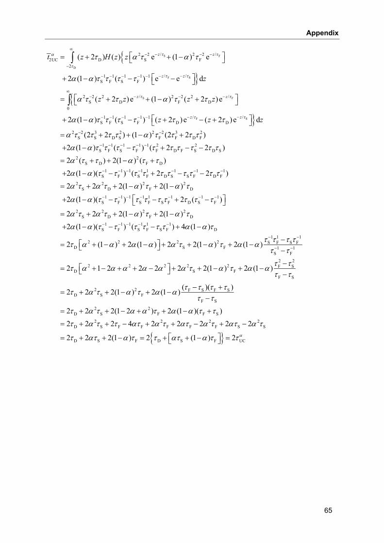
Appendix
65
{
}{
S F
D
SF
S F
/ /2 2 2 22UC D S F
2
//1 1 1 1 1S F S F
/ /2 2 2 2 2 2S D F D
0
/1 1 1 1 1S F S F D
( 2 ) ( ) e (1 ) e
2 (1 ) ( ) e e d
( 2 )e (1 ) ( 2 )e
2 (1 ) ( ) ( 2 )e
τ τα
τ
ττ
τ τ
τ α τ α τ
α α τ τ τ τ
α τ τ α τ τ
α α τ τ τ τ τ
∞− −− −
−
−−− − − − −
∞− −− −
−− − − − −
⎡ ⎤= + + −⎣ ⎦
⎡ ⎤+ − − −⎣ ⎦
⎡ ⎤= + + − +⎣ ⎦
+ − − +
∫
∫
z z
zz
z z
z
t z H z z
z
z z z z
z }SF /D
2 2 3 2 2 2 3 2S S D S F F D F
1 1 1 1 1 2 2S F S F F D F S D S
2 2S D F D
1 1 1 1 1 1 1 1S F S F D S S F D F
2
( 2 )e d
(2 2 ) (1 ) (2 2 )
2 (1 ) ( ) ( 2 2 )
2 ( ) 2(1 ) ( )
2 (1 )( ) ( 2 2 )
2
ττ τ
α τ τ τ τ α τ τ τ τ
α α τ τ τ τ τ τ τ τ τ τ
α τ τ α τ τ
α α τ τ τ τ τ τ τ τ τ τ
α τ
−
− −
− − − − −
− − − − − − −
⎡ ⎤− +⎣ ⎦
= + + − +
+ − − + − −
= + + − +
+ − − + − −
=
zz z
2 2 2S D F D
1 1 1 1 1 1 1 1S F S F S F D S F
2 2 2 2S D F D
1 1 1 1 1 1S F S F S F D
2 2 2 2D S
2 2(1 ) 2(1 )
2 (1 )( ) 2 ( )
2 2 2(1 ) 2(1 )
2 (1 )( ) ( ) 4 (1 )
2 (1 ) 2 (1 ) 2 2(1 )
α τ α τ α τ
α α τ τ τ τ τ τ τ τ τ
α τ α τ α τ α τ
α α τ τ τ τ τ τ α α τ
τ α α α α α τ α τ
− − − − − − −
− − − − −
+ + − + −
⎡ ⎤+ − − − + −⎣ ⎦= + + − + −
+ − − − + −
⎡ ⎤= + − + − + + −⎣ ⎦1 1 1
S F S FF 1 1
S F
2 22 2 2 2 2 F S
D S FF S
2 2 F S F SD S F
F S2 2
D S F F S2
D S F F
2 (1 )
2 1 2 2 2 2 2(1 ) 2 (1 )
( )( )2 2 2(1 ) 2 (1 )
2 2 2(1 2 ) 2 (1 )( )
2 2 2 4 2
τ τ τ τα ατ τ
τ ττ α α α α α α τ α τ α ατ τ
τ τ τ ττ α τ α τ α ατ τ
τ α τ α α τ α α τ τ
τ α τ τ ατ α
− −
− −
−+ −
−
−⎡ ⎤= + − + + − + + − + −⎣ ⎦ −
− += + + − + −
−
= + + − + + − +
= + + − +
{ }2 2 2
F F F S S
D S F D S F UC
2 2 2 2
2 2 2(1 ) 2 (1 ) 2 α
τ ατ α τ ατ α τ
τ ατ α τ τ ατ α τ τ
+ − + −
⎡ ⎤= + + − = + + − =⎣ ⎦

Appendix
66
Appendix C. Evaluations by Laplace transformation The unit cell RTD of the PD model is given by
D DUC
S S
( )( ) expH t tE t τ ττ τ
⎛ ⎞− −= −⎜ ⎟
⎝ ⎠ (77)
and that of the PDD model by
D DUC D D
S S F F
1( ) ( ) exp ( ) expt tE t H t H tα τ τα ατ ττ τ τ τ
⎛ ⎞ ⎛ ⎞− −−= − − + − −⎜ ⎟ ⎜ ⎟
⎝ ⎠⎝ ⎠ (78)
The Laplace transform of Eq. (77) is
D
D
D DUC UC
S S0 0
S D S DD
S S S S0
SD
S S S
D
S S
( )( ) exp( ) ( )d exp( ) exp d
(1 ) (1 )( ) 1exp d exp d
(1 )1 exp exp d
1 exp exp
H t tE s st E t t st t
t s t sH t t t
t s t
τ
τ
τ ττ τ
τ τ τ τττ τ τ τ
τττ τ τ
ττ τ
∞ ∞
∞ ∞
∞
⎛ ⎞− −= − = − −⎜ ⎟
⎝ ⎠⎛ ⎞ ⎛ ⎞+ − + −−
= − = −⎜ ⎟ ⎜ ⎟⎝ ⎠ ⎝ ⎠
⎛ ⎞ ⎛ ⎞+= −⎜ ⎟ ⎜ ⎟
⎝ ⎠ ⎝ ⎠
⎛ ⎞= −⎜ ⎟
⎝ ⎠
∫ ∫
∫ ∫
∫
( )
D D
S S SD
S S S S S
S D S D SD D
S S S S S S S
D 1S S S
(1 ) (1 )1 exp exp1
(1 ) (1 )1 1exp exp exp1 1
1 1 1exp exp1
t t
t t
t s t ss
s ss s
ss s
τ τ
τ τ τττ τ τ τ τ
τ τ τ τ ττ ττ τ τ τ τ τ τ
ττ τ τ
=∞ =∞
= =
−
⎡ ⎤ ⎡ ⎤⎛ ⎞ ⎛ ⎞ ⎛ ⎞+ += − −⎢ ⎥ ⎢ ⎥⎜ ⎟ ⎜ ⎟ ⎜ ⎟+⎝ ⎠ ⎝ ⎠ ⎝ ⎠⎣ ⎦ ⎣ ⎦
⎡ ⎤⎛ ⎞ ⎛ ⎞ ⎛ ⎞+ += − = − +⎢ ⎥⎜ ⎟ ⎜ ⎟ ⎜ ⎟+ +⎝ ⎠ ⎝ ⎠ ⎝ ⎠⎣ ⎦
= − = −+ +
( )Dsτ
Then, the Laplace transform of Eq. (78) is
( ) ( )UC UC D D1 1S S F F0
1 1 1( ) exp( ) ( )d exp expE s st E t t s ss s
α α α ατ ττ τ τ τ
∞
− −
−= − = − + −
+ +∫ (79)
The RTD for 2 unit cells in series is given by the convolution
2UC UC UC( ) ( ) ( )E t E t E tα α α= ∗
In the Laplace domain this gives

Appendix
67
( ) ( )
( )
22
2UC UC UC UC D D1 1S S F F
2
D1 1S S F F
1 1 1( ) ( ) ( ) ( ) exp exp
1 1 1 exp 2
E s E s E s E s s ss s
ss s
α α α α α ατ ττ τ τ τ
α α ττ τ τ τ
− −
− −
⎡ ⎤−⎡ ⎤= ⋅ = = − + −⎢ ⎥⎣ ⎦ + +⎣ ⎦
⎛ ⎞−= + −⎜ ⎟+ +⎝ ⎠
The RTD for n unit cells in series is given by the convolution
UC ( 1)UC UC( ) ( ) ( )n nE t E t E tα α α−= ∗
In the Laplace domain this gives
( )UC UC D1 1S S F F
1 1 1( ) ( ) expn
n
nE s E s n ss s
α α α α ττ τ τ τ− −
⎛ ⎞−⎡ ⎤= = + −⎜ ⎟⎣ ⎦ + +⎝ ⎠ (80)
For the PD model, it is 1α = and Eq. (80) simplifies to
( ) ( )UC S D D1S S
1 1( ) (1 ) exp exp( )
nn n nE s s n s n s
sτ τ τ
τ τ−
−= + − = −+
(81)
The backward transformation in the time domain of Eq. (81) is
1D D
UC DS S
( )( ) exp ( )( 1)!
n
n n
t n t nE t H t nn
τ τ ττ τ
− ⎛ ⎞− −= − −⎜ ⎟− ⎝ ⎠
see ID 2 (delayed nth power with frequency shift) in the Table of selected Laplace transforms
in the English Wikipedia web site on Laplace transformation (accessed June, 2009).
To determine the inverse of Eq. (80) we take advantage of the binomial theorem which reads
0
( ) −
=
⎛ ⎞+ = ⎜ ⎟
⎝ ⎠∑
nn n k k
k
na b a b
k
In the present case n and k are positive integers. Then, for ≥n k the binomial coefficients
are given by
!!( )!
n nk k n k⎛ ⎞
=⎜ ⎟ −⎝ ⎠
Introducing these results in Eq. (80) gives
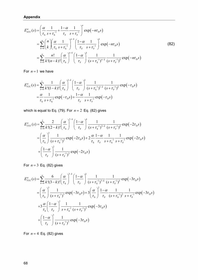
Appendix
68
( )
( )
( )
UC D1 1S S F F
D1 10 S S F F
D1 10 S F S F
1 1 1( ) exp
1 1 1 exp
! 1 1 1 exp!( )! ( ) ( )
n
n
n k kn
k
n k kn
n k kk
E s n ss s
nn s
k s s
n n sk n k s s
α α α ττ τ τ τ
α α ττ τ τ τ
α α ττ τ τ τ
− −
−
− −=
−
− − −=
⎛ ⎞−= + −⎜ ⎟+ +⎝ ⎠
⎛ ⎞ ⎛ ⎞⎛ ⎞ −= −⎜ ⎟ ⎜ ⎟⎜ ⎟ + +⎝ ⎠ ⎝ ⎠⎝ ⎠
⎛ ⎞ ⎛ ⎞−= −⎜ ⎟ ⎜ ⎟− + +⎝ ⎠⎝ ⎠
∑
∑
(82)
For 1=n we have
( )
( ) ( )
11
1UC D1 1 10 S F S F
D D1 1S S F F
1 1 1 1( ) exp!(1 )! ( ) ( )1 1 1exp exp
k k
k kk
E s sk k s s
s ss s
α α α ττ τ τ τ
α ατ ττ τ τ τ
−
− − −=
− −
⎛ ⎞ ⎛ ⎞−= −⎜ ⎟ ⎜ ⎟− + +⎝ ⎠⎝ ⎠
−= − + −
+ +
∑
which is equal to Eq. (79). For 2=n Eq. (82) gives
( )
( ) ( )
( )
22
2UC D1 2 10 S F S F
2
D D1 2 1 1S S S F S F
2
D1 2F F
2 1 1 1( ) exp 2!(2 )! ( ) ( )
1 1 1 1exp 2 2 exp 2( )
1 1 exp 2( )
k k
k kk
E s sk k s s
s ss s s
ss
α α α ττ τ τ τ
α α ατ ττ τ τ τ τ τ
α ττ τ
−
− − −=
− − −
−
⎛ ⎞ ⎛ ⎞−= −⎜ ⎟ ⎜ ⎟− + +⎝ ⎠⎝ ⎠
⎛ ⎞ −= − + −⎜ ⎟ + + +⎝ ⎠
⎛ ⎞−+ −⎜ ⎟ +⎝ ⎠
∑
For 3n = Eq. (82) gives
( )
( ) ( )
( )
3
3UC D1 3 10 S F S F
3 2
D D1 3 1 2 1S S S F S F
2
D1 1 2S F S F
F
6 1 1 1( ) exp 3!(3 )! ( ) ( )
1 1 1 1exp 3 3 exp 3( ) ( )
1 1 13 exp 3( )
1
k kn
k kk
E s sk k s s
s ss s s
ss s
α α α ττ τ τ τ
α α ατ ττ τ τ τ τ τ
α α ττ τ τ τ
ατ
−
− − −=
− − −
− −
⎛ ⎞ ⎛ ⎞−= −⎜ ⎟ ⎜ ⎟− + +⎝ ⎠⎝ ⎠
⎛ ⎞ ⎛ ⎞ −= − + −⎜ ⎟ ⎜ ⎟+ + +⎝ ⎠ ⎝ ⎠
⎛ ⎞−+ −⎜ ⎟ + +⎝ ⎠
⎛ ⎞−+⎜⎝
∑
( )3
D1 3F
1 exp 3( )
ss
ττ − −⎟ +⎠
For 4n = Eq. (82) gives
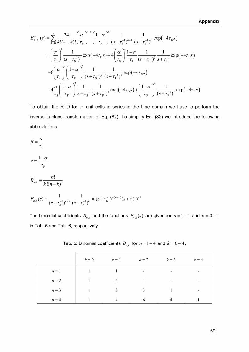
Appendix
69
( )
( ) ( )
4
4UC D1 4 10 S F S F
4 3
D D1 4 1 3 1S S S F S F
2 2
D1 2 1 2S F S F
24 1 1 1( ) exp 4!(4 )! ( ) ( )
1 1 1 1exp 4 4 exp 4( ) ( )
1 1 16 exp 4( ) ( )
k kn
k kk
E s sk k s s
s ss s s
s s
α α α ττ τ τ τ
α α ατ ττ τ τ τ τ τ
α α ττ τ τ τ
−
− − −=
− − −
− −
⎛ ⎞ ⎛ ⎞−= −⎜ ⎟ ⎜ ⎟− + +⎝ ⎠⎝ ⎠
⎛ ⎞ ⎛ ⎞ −= − + −⎜ ⎟ ⎜ ⎟+ + +⎝ ⎠ ⎝ ⎠
⎛ ⎞ ⎛ ⎞−+ −⎜ ⎟ ⎜ ⎟ + +⎝ ⎠⎝ ⎠
∑
( )
( ) ( )3 4
D D1 1 3 1 4S F S F F F
1 1 1 1 14 exp 4 exp 4( ) ( )
s
s ss s s
α α ατ ττ τ τ τ τ τ− − −
⎛ ⎞ ⎛ ⎞− −+ − + −⎜ ⎟ ⎜ ⎟+ + +⎝ ⎠ ⎝ ⎠
To obtain the RTD for n unit cells in series in the time domain we have to perform the
inverse Laplace transformation of Eq. (82). To simplify Eq. (82) we introduce the following
abbreviations
S
αβτ
≡
F
1 αγτ−
≡
,!
!( )!n knB
k n k≡
−
1 ( ) 1, S F1 1
S F
1 1( ) ( ) ( )( ) ( )
n k kn k n k kF s s s
s sτ τ
τ τ− − − − −
− − −≡ = + ++ +
The binomial coefficients ,n kB and the functions , ( )n kF s are given for 1 4n = − and 0 4k = −
in Tab. 5 and Tab. 6, respectively.
Tab. 5: Binomial coefficients ,n kB for 1 4n = − and 0 4k = − .
k = 0 k = 1 k = 2 k = 3 k = 4
n = 1 1 1 - - -
n = 2 1 2 1 - -
n = 3 1 3 3 1 -
n = 4 1 4 6 4 1

Appendix
70
Tab. 6: Functions , ( )n kF s for 1 4n = − and 0 4k = − .
k = 0 k = 1 k = 2 k = 3 k = 4
n=1 1 1S( )s τ − −+ 1 1
F( )s τ − −+ - - -
n=2 1 2S( )s τ − −+ 1 1 1 1
S F( ) ( )s sτ τ− − − −+ + 1 2F( )s τ − −+ - -
n=3 1 3S( )s τ − −+ 1 2 1 1
S F( ) ( )s sτ τ− − − −+ + 1 1 1 2S F( ) ( )s sτ τ− − − −+ + 1 3
F( )s τ − −+ -
n=4 1 4S( )s τ − −+ 1 3 1 1
S F( ) ( )s sτ τ− − − −+ + 1 2 1 2S F( ) ( )s sτ τ− − − −+ + 1 1 1 3
S F( ) ( )s sτ τ− − − −+ + 1 4F( )s τ − −+
Then Eq. (82) can be written as
( )UC , , D0
( ) ( ) expn
n k kn n k n k
kE s B F s n sα β γ τ−
=
= −∑ (83)
The inverse of Eq. (83) is given by
( ){ } ( ){ }1 1UC , , D , , D
0 0( ) ( ) exp ( )exp
n nn k k n k k
n n k n k n k n kk k
E t B F s n s B F s n sα β γ τ β γ τ− − − −
= =
= − = −∑ ∑L L (84)
Taking advantage of the following time shift property of the Laplace transform
( ){ }1 ( ) exp ( ) ( )F s as f t a H t a− − = − −L
Eq. (84) simplifies to
UC D , , D0
( ) ( ) ( )n
n k kn n k n k
kE t H t n B f t nα τ β γ τ−
=
= − −∑ (85)
where
{ }1, ,( ) ( )n k n kf t F s−≡ L
To determine the inverse Laplace transforms we take advantage of the relations listed in
Tab. 7.

Appendix
71
Tab. 7: Inverse Laplace transforms. In the reference column the numbers refer to those in
McCollum and Brown (1965), CB, and Roberts and Kaufman (1966), RK, respectively.
( )F s ( )f t Reference
( ) ns a −+ 1 exp( )( 1)!
nt atn
− −−
23 in CB
1 1( ) ( )s a s b− −+ + [ ]1 exp( ) exp( )at btb a
− − −−
14 in CB
1 2( ) ( )s a s b− −+ + [ ]{ }2
1 exp( ) ( ) 1 exp( )( )
at a b t bta b
− + − − −−
27 in CB
2 2( ) ( )s a s b− −+ + 2 3 2 3
exp( ) 2exp( ) exp( ) 2exp( )( ) ( ) ( ) ( )
t at at t bt btb a b a a b a b
− − − −− + −
− − − − 33 in CB
1 3( ) ( )s a s b− −+ + 2 2
3
1 11 ( ) ( ) exp( ) exp( )( ) 2
a b t a b t bt ata b
⎧ ⎫⎡ ⎤− − + − − − −⎨ ⎬⎢ ⎥− ⎣ ⎦⎩ ⎭ 89 of sec-
tion 2 in RK
With the above results, the inverse Laplace transforms of , ( )n kF s for 1 4n = − and 0 4k = −
are as follows
11,0 S( ) exp( )f t tτ −= −
11,1 F( ) exp( )f t tτ −= −
12,0 S( ) exp( )f t t tτ −= −
1 12,1 S F1 1
F S
1( ) exp( ) exp( )f t t tτ ττ τ
− −− −
⎡ ⎤= − − −⎣ ⎦−
12,2 F( ) exp( )f t t tτ −= −
21
3,0 S( ) exp( )2tf t tτ −= −
1 1 11F S SF
3,1 1 1 2 1 1 2F S F S
( ) 1 exp( )exp( )( )( ) ( )
t ttf tτ τ ττ
τ τ τ τ
− − −−
− − − −
⎡ ⎤− − −− ⎣ ⎦= +− −
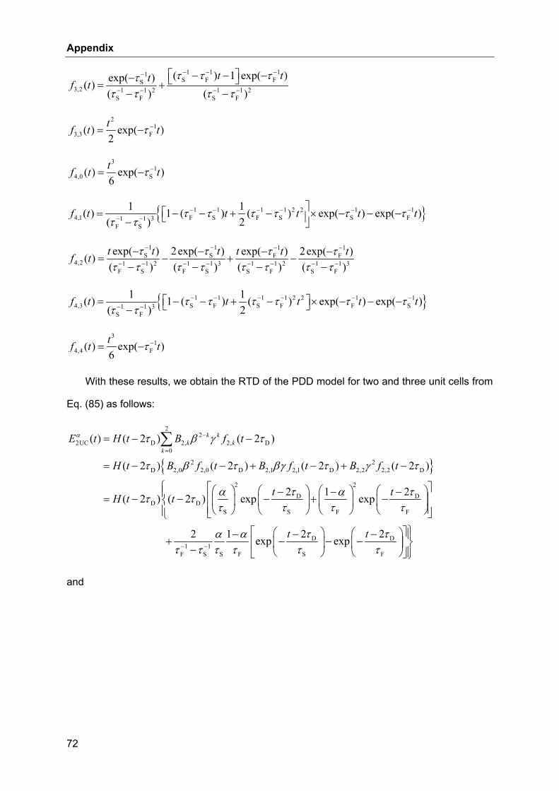
Appendix
72
1 1 11S F FS
3,2 1 1 2 1 1 2S F S F
( ) 1 exp( )exp( )( )( ) ( )
t ttf tτ τ ττ
τ τ τ τ
− − −−
− − − −
⎡ ⎤− − −− ⎣ ⎦= +− −
21
3,3 F( ) exp( )2tf t tτ −= −
31
4,0 S( ) exp( )6tf t tτ −= −
{ }1 1 1 1 2 2 1 14,1 F S F S S F1 1 3
F S
1 1( ) 1 ( ) ( ) exp( ) exp( )( ) 2
f t t t t tτ τ τ τ τ ττ τ
− − − − − −− −
⎤⎡= − − + − × − − −⎣ ⎥− ⎦
1 1 1 1S S F F
4,2 1 1 2 1 1 3 1 1 2 1 1 3F S F S S F S F
exp( ) 2exp( ) exp( ) 2exp( )( )( ) ( ) ( ) ( )t t t t t tf t τ τ τ ττ τ τ τ τ τ τ τ
− − − −
− − − − − − − −
− − − −= − + −
− − − −
{ }1 1 1 1 2 2 1 14,3 S F S F F S1 1 3
S F
1 1( ) 1 ( ) ( ) exp( ) exp( )( ) 2
f t t t t tτ τ τ τ τ ττ τ
− − − − − −− −
⎡ ⎤= − − + − × − − −⎣ ⎦−
31
4,4 F( ) exp( )6tf t tτ −= −
With these results, we obtain the RTD of the PDD model for two and three unit cells from
Eq. (85) as follows:
{ }
22
2UC D 2, 2, D0
2 2D 2,0 2,0 D 2,1 2,1 D 2,2 2,2 D
2 2
D DD D
S S F F
1F S
( ) ( 2 ) ( 2 )
( 2 ) ( 2 ) ( 2 ) ( 2 )
2 21( 2 ) ( 2 ) exp exp
2
k kk k
kE t H t B f t
H t B f t B f t B f t
t tH t t
α τ β γ τ
τ β τ βγ τ γ τ
τ τα ατ ττ τ τ τ
τ τ
−
=
−
= − −
= − − + − + −
⎧ ⎡ ⎤⎛ ⎞ ⎛ ⎞ ⎛ ⎞ ⎛ ⎞− −−⎪ ⎢ ⎥= − − − + −⎨ ⎜ ⎟ ⎜ ⎟ ⎜ ⎟ ⎜ ⎟⎢ ⎥⎝ ⎠ ⎝ ⎠⎝ ⎠ ⎝ ⎠⎪ ⎣ ⎦⎩
+−
∑
D D1
S F S F
2 21 exp expt tτ τα ατ τ τ τ−
⎫⎡ ⎤⎛ ⎞ ⎛ ⎞− −− ⎪− − − ⎬⎢ ⎥⎜ ⎟ ⎜ ⎟⎝ ⎠⎝ ⎠ ⎪⎣ ⎦⎭
and
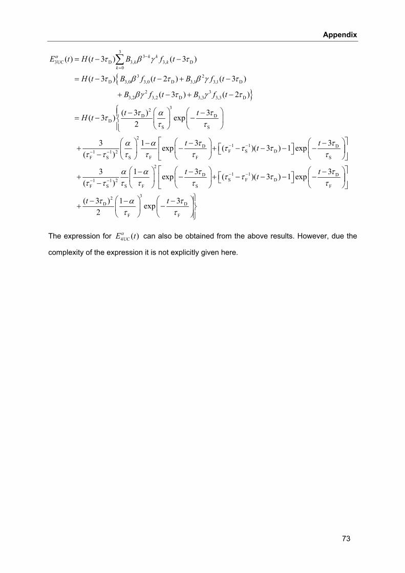
Appendix
73
{}
33
3UC D 3, 3, D0
3 2D 3,0 3,0 D 3,1 3,1 D
2 33,2 3,2 D 3,3 3,3 D
32D D
DS S
2
1 1 2F S S
( ) ( 3 ) ( 3 )
( 3 ) ( 2 ) ( 3 )
( 3 ) ( 2 )
( 3 ) 3( 3 ) exp2
3 1( )
k kk k
k
E t H t B f t
H t B f t B f t
B f t B f t
t tH t
α τ β γ τ
τ β τ β γ τ
βγ τ γ τ
τ ταττ τ
ατ τ τ
−
=
− −
= − −
= − − + −
+ − + −
⎧ ⎛ ⎞ ⎛ ⎞− −⎪= − −⎨ ⎜ ⎟ ⎜ ⎟⎝ ⎠ ⎝ ⎠⎪⎩
⎛ ⎞+ ⎜ ⎟− ⎝ ⎠
∑
1 1D DF S D
F F S
21 1D D
S F D1 1 2F S S F S F
32D D
F F
3 3exp ( )( 3 ) 1 exp
3 33 1 exp ( )( 3 ) 1 exp( )
( 3 ) 31 exp2
t tt
t tt
t t
τ τα τ τ ττ τ τ
τ τα α τ τ ττ τ τ τ τ τ
τ τατ τ
− −
− −− −
⎡ ⎤⎛ ⎞⎛ ⎞− −− ⎡ ⎤− + − − − −⎢ ⎥⎜ ⎟⎜ ⎟ ⎣ ⎦⎝ ⎠ ⎝ ⎠⎣ ⎦
⎡ ⎤⎛ ⎞⎛ ⎞ ⎛ ⎞− −− ⎡ ⎤+ − + − − − −⎢ ⎥⎜ ⎟⎜ ⎟ ⎜ ⎟⎣ ⎦− ⎝ ⎠ ⎝ ⎠⎝ ⎠⎣ ⎦
⎛ ⎞ ⎛ ⎞− −−+ −⎜ ⎟ ⎜
⎝ ⎠ ⎝
⎫⎪⎬⎟⎠⎪⎭
The expression for 4UC ( )E tα can also be obtained from the above results. However, due the
complexity of the expression it is not explicitly given here.