Olli-Pekka Lehto – CSC, IT Center for Science

Numerical Libraries

PRACE workshop on application porting and performance tuning 11.6.2009, Espoo, Finland

Contents

• Overview of current numerical libraries– Brief introduction and basic usage

– Performance measurements– Best practices

• Focus on libraries for the Cray XT -series– Largely based on freely available libraries and standard interfaces

• Available for other platforms as well

• Additional enhancements by Cray

– CSC's capability HPC system: louhi.csc.fi• Cray XT4/XT5 MPP system with a 3D torus interconnect

• ~100TFlop/s

• 2 XT5 cabinets (1440 AMD Shanghai cores) dedicated for PRACE use

Numerical Libraries – Application Areas

• Linear Algebra– Systems of equations

• Direct vs. Iterative solvers

• Sparse vs. Dense system

– Eigenvalue problems• Few of the largest / smallest / all

– Least squares

• Optimization– Linear vs. Nonlinear

– Global vs. Local minimum

– Bounded vs. Unbounded

• Signal processing– FFT

• Numerical Integration– Quadrature

– N-Dimensional cases

– Special topologies (spheres etc.)

• Interpolation and Approximation

• Random Number Generators

• Statistics

• Ordinary Differential Equations

• Partial Differential Equations– Usually with suites leveraging a

combination of lower level libraries

• Preprocessing– Preconditioners, decomposers

Numerical libraries – Motivation for Use

• No need to reinvent the wheel• Improves structuring of program code• Code is likely to be well-tested & optimized• May enhance portability

– Provided that the libraries are portable

• Makes performance prediction easier– “What type of architecture would the best choice for this code?”

Numerical libraries - Types

• Common, standardized APIs (for example, BLAS) have a number of implementations – Reference (Netlib BLAS, numerical recipes etc.)– Multiplatform, optimized implementations

• Free, community developed (ATLAS etc.)• Commercial (IMSL, NAG etc.)

– Vendor-optimized architecture-specific (AMD ACML, Intel MKL etc.)

• Many classes of libraries do not have a standardized interface– For example: FFT, RNG

Criteria for Choosing a Library

• Applicability to the task

• Performance

• Reliability

• Accuracy– (vs. performance)

• Ease of use

• Continuity of development

• Pricing• Licensing

– Redistribution of programs

• Maintenance cost/ease• Supported languages• Supported platforms• Parallelization (if needed)

Optimization Strategies for Numerical Libraries

• Algorithmic optimization• Utilization of special instruction sets

– SSE, 3DNow!, Altivec etc.

• Trade off accuracy and reliability for speed– Mixed-precision – Relaxed precision– Reduce error checking

• Optimized cache usage• Optimized communication patterns in parallel libraries• Autotuning

Autotuning• Optimization based on running a set of benchmarks

– Find the best implementation/algorithm/parameter set for a specific architecture and/or input

• Benefits– Makes the libraries easier to port

– Reduces the complexity of the API (less function parameters)

– May even outperform vendor libraries

– Optimization based on input data is important for some problem classes

• Autotuning benchmarks (probes) may be run in different stages– During compilation

– At runtime

– Using a separate benchmark program to create a configuration file

• Can be problematic in cross-compiling environments – For example: Cray XT, IBM BlueGene

– Probes need to be executed on the compute node, not on the frontend

• Examples of autotuning libraries: ATLAS, FFTW, CASK

Scientific Libraries on Cray XT

• Sparse systems– PETSc

• Hypre• ParMETIS• MUMPS • SuperLU (LibSci)• SuperLU_dist (LibSci)• CASK (LibSci)

• Intrinsic functions– ACML-MV (ACML)– Fast-MV (LibSci)

• Linear algebra– BLAS (LibSci, ACML)– LAPACK (LibSci, ACML)– ScaLAPACK (LibSci)– IRT (LibSci)

• FFT– FFTW– ACML FFT (ACML) – CRAFFT (LibSci)

• Random number generator– ACML RNG (ACML)

Library suites - Cray LibSci

• Current version: 10.3.5

• Contents: – Optimized Implementations of standard shared- and distributed memory libraries

• BLAS, PBLAS, LAPACK, ScaLAPACK

– Fast math intrinsics

• Fast-MV

– Cray libraries

• IRT, CRAFFT, CASK

– Sparse systems

• SuperLU

• To usemodule load xt-libsci (Loaded on Louhi by default)

• Usage Instructions• man intro_libsci

• Cray XT Programming Environment User's Guide (via scientist's interface)

– http://docs.cray.com

Library Suites - AMD ACML

• Current version: 4.2.0• Contents

– Optimized Implementations of standard shared-memory libraries• BLAS, LAPACK

– Random nubmer generators: • ACML RNG

– Fast math intrinsics• ACML-MV

• To use:module load acml

• Instructions:• AMD ACML User's Guide

– http://developer.amd.com/cpu/Libraries/acml

Dense Linear Algebra Libraries

• The “Netlib” libraries have become a de facto standard for dense linear algebra– Most notably: BLAS, LAPACK, BLACS, PBLAS, ScaLAPACK – Originally developed at University of Tennessee – Reference implementations available freely from

http://www.netlib.org/

• A number of optimized implementations are available– On Louhi: AMD ACML, Cray LibSci– Other open-source, cross-platform: ATLAS, LibGOTO ...– Other proprietary: Intel MKL, IBM ESSL ...

BLAS - Basic Linear Algebra Subroutines

• Basic dense matrix operations– Multiplication, addition, rank update, solving triangular matrices

• Sequential or shared memory parallel– Some implementations have multithreading support

• Functionality divided into 3 levels– Level 1: Vector operations (1979)– Level 2: Matrix-vector operations (1986)– Level 3: Matrix-matrix operations (1988, updated in 2002)

• Reference implementations in Fortran and C– Netlib BLAS http://www.netlib.org/blas/

BLAS: Anatomy of a BLAS call

• Fortran and C• Naming convention: X YYY ZZZZ(parameters)

– X • Precision: Real, Double, Complex, Z complex double

• Some routines can have combined codes (e.g. scasum)

– Y• Level 1 operation type: DOT product, ROTate, SWAP, etc.• Level 2&3 matrix type: SYmmetric, GEneral, HErmitian etc.

– Z • Additional details, for example:

C = Conjugated vector (L1)MV = Matrix-Vector product (L2)MM = Matrix Multiply (L3)

BLAS: Example

DGEMM(transa, transb, l, n, m, alpha, a, lda, b, ldb, beta, c, ldc)

Double precision GEneral Matrix Multiply

• a, b = input matrices

• c = output matrix

• transa/transb = Form of the input matrix– 'N' Normal or 'T' Transpose

• l, n = rows, columns of output matrix c

• m = columns of a, rows of b if neither is transposed– Transpose: columns ↔ rows

• alpha, beta = scaling constants

• lda, ldb, ldc = Leading dimensions of the arrays

C ← αAB+βC

On Louhi:Included in Cray LibSci

BLAS Performance Measurements

• BLAS performance is important– Widely used in a number of codes– A foundation for many higher level libraries

• Evaluation of 3 BLAS routines on Louhi – DAXPY – Level 1 vector-vector sum– DGEMV – Level 2 vector-matrix multiply– DGEMM – Level 3 matrix-matrix multiply

• Comparison of different BLAS implementations – AMD ACML– LibSci– libGoto 1.26– Intel MKL 10.1.015– Netlib BLAS (“Reference BLAS”)

DAXPY - Vector-vector Addy ← αx+y

DGEMV – Matrix Vector Multiplyy ← αAx+βy

DGEMM – Matrix-matrix Multiply C ← αAB+βC

ACML Threaded BLAS

• ACML supports OpenMP shared memory parallelization for level 3 BLAS routines

• Usage on Louhi– Link using OpenMP flags and the libacml_mp.a library

– Use the OMP_NUM_THREADS environment variable and use the -d option with aprun to set the thread count

ACML Threaded BLAS SpeedupDGEMM speedup with multiple threads

ACML Threaded BLAS EfficiencyDGEMM parallel efficiency with multiple threads

Perfectscaling

LAPACK - Linear Algebra PACKage

• Matrix solvers– Simultaneous linear equations, Least-squares solutions,

Eigenvalue problems, Singular value problems– Matrix factorizations (LU, Cholesky, QR, SVD, Schur)

• Sequential or shared memory parallel– Some implementations have multithreading support

• Leverages BLAS– Computation is largely performed by calls to BLAS– Similar nomenclature to BLAS

• 1. Precision 2. Matrix type 3. Operation

• For example: DGESV = Double precision, GEneral matrix, Solve

http://www.netlib.org/lapack/

On Louhi:Included in Cray LibSci and ACML

LAPACK: DGESVSolve AX=B

LAPACK: DGEEVFind Eigenvalues for matrix

LAPACK: DGELSFind a linear least squares solution for a matrix

BLACS - Basic Linear Algebra Communication Subroutines• Decomposes a matrix onto a process grid

– 1- or 2-dimensional

• Addresses frequently occurring operations in linear algebra– Hides complexities of the underlying

communication library (MPI, PVM etc.)– Scoped broadcast operations

• e.g. “Transfer this data to all processes in a column”

– Element-wise SUM, |MAX|,|MIN| ops on triangular matrices

On Louhi:Included in Cray LibSci

0 1 2

0 0 1 2

1 3 4 5

3x4 Process Grid

http://www.netlib.org/blacs/

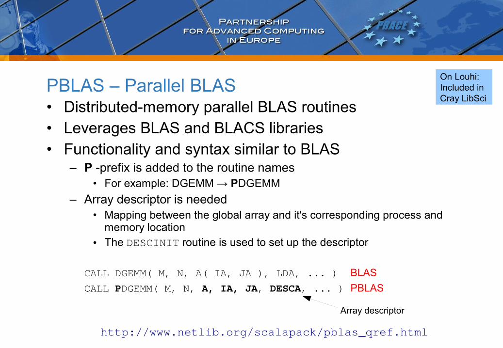
PBLAS – Parallel BLAS• Distributed-memory parallel BLAS routines• Leverages BLAS and BLACS libraries• Functionality and syntax similar to BLAS

– P -prefix is added to the routine names• For example: DGEMM → PDGEMM

– Array descriptor is needed• Mapping between the global array and it's corresponding process and

memory location

• The DESCINIT routine is used to set up the descriptor

CALL DGEMM( M, N, A( IA, JA ), LDA, ... ) BLAS

CALL PDGEMM( M, N, A, IA, JA, DESCA, ... ) PBLAS

On Louhi:Included in Cray LibSci

Array descriptor

http://www.netlib.org/scalapack/pblas_qref.html

ScaLAPACK – Scalable LAPACK

• Parallel LAPACK routines– Dense and banded matrices

• Leverages a number of libraries– MPI, BLAS, BLACS, LAPACK, PBLAS

• Functionality and syntax similar to LAPACK– With P prefix and array descriptor

CALL DGESV( N, NRHS, A( I, J ), LDA, ... ) LAPACK

CALL PDGESV( N, NRHS, A, I, J, DESCA, ... ) ScaLAPACK

http://www.netlib.org/scalapack

PBLAS/ScaLAPACK decomposition

• PBLAS and ScaLAPACK decompose the matrix into smaller submatrices– The style of decomposition affects the performance

characteristics

• By default, 2-dimensional block-cyclic parallelization is used– Blocks of elements (block size NB) are distributed in

an interleaved fashion on the process grid– Ensures reasonable load balancing even when

working with partially filled matrices– The process grid dimensions and block size have

2-dimensionalBlock distribution2x2 Process grid

NB = 1/8*N

ScaLAPACK Process Grid Topology64P LU Factorization performance using

different process grid topologies

ScaLAPACK Block Size

64P LU Factorization performance as a function of block size (NB) using different sizes

Using ScaLAPACK

1) Initialize the processor grid with BLACSSL_INIT

BLACS_GRIDINFO

2) Distribute the matrix on the processor grid• Distribute the matrix• Have each process initialize an array descriptor

DESCINIT

• Have each process initialize its local arrayPCELSET, PSELSET or PCELSET

3) Call the ScaLAPACK routineFor example, PDGESV

4) Release the processor gridBLACS_GRIDEXIT

BLACS_EXIT

Message Passing(MPI, PVM etc.)

BLACS

PBLAS

LAPACK

ScaLAPACK

Local addressing

Global addressing

BLAS

Dense Linear Algebra Libraries:An Overview

Platform-specific

Sequentialor shared memory

Distributed memory

Basic BLAS PBLAS

Advanced LAPACK ScaLAPACK

Cray IRT – Iterative Refinement Toolkit

• Library of dense linear solvers using iterative precision refinement– Uses fast single precision factorizations as much as possible

– Solutions accurate to double precision

• Max. Theoretical speed-up 2x, in practice 1.2-1.7x– Depends on the condition number (lower is better)

• Serial and parallel versions of factorization routines– LU, Cholesky, QR (serial-only)

• Two ways to use the API– Automatic IRT routines

• Set the environment variable: IRT_USE_SOLVERS=1

• IRT used automatically with existing ScaLAPACK/LAPACK factorization routines

– Advanced IRT API• Existing routines need to be changed to IRT routines

• Greater control over iteration parameters

On Louhi:Included in Cray LibSci

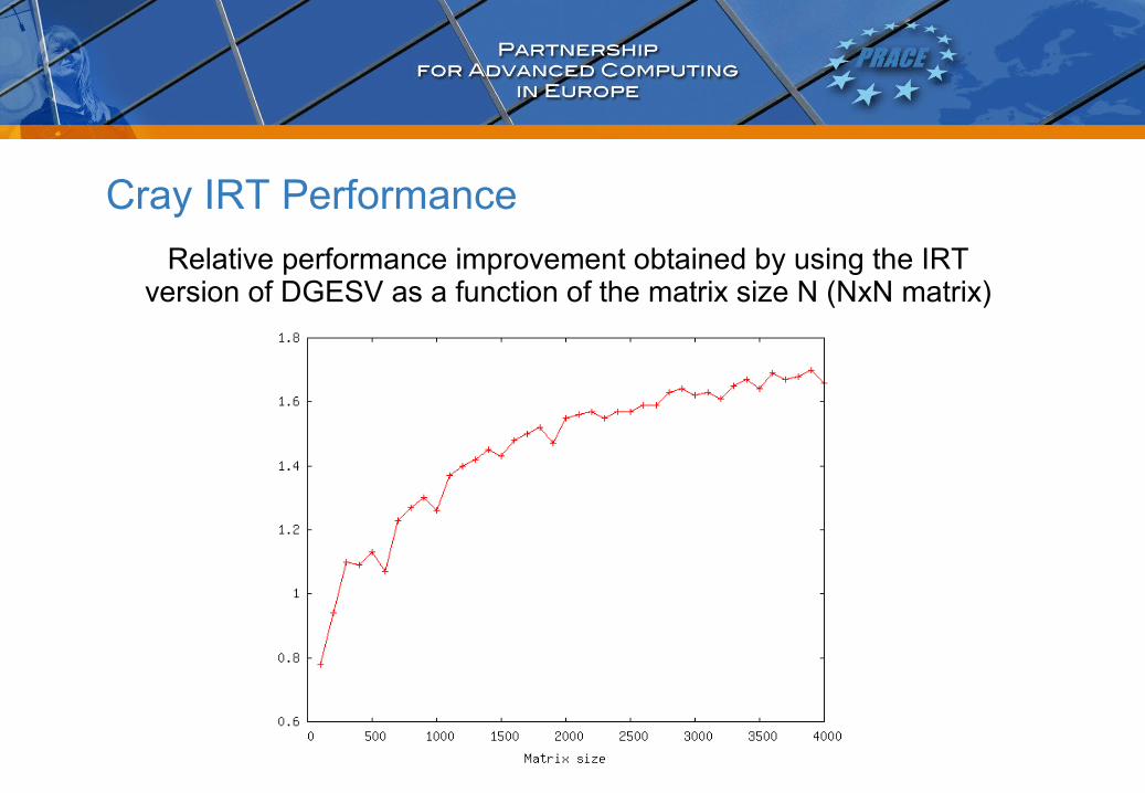
Cray IRT Performance

Relative performance improvement obtained by using the IRT version of DGESV as a function of the matrix size N (NxN matrix)

FFT Libraries

• 3 FFT libraries supported on Cray XT– FFTW

– ACML FFT

– CRAFFT

• No common API– Different implementations have different interfaces

• Functionally relatively similar (2 step process)1. Create a “plan”

• Description of the combination of codelets to be used to compute the FFT

2. Execute the FFT

• Array sizes of powers of 2 tend to yield good performance

• Other interesting libraries (unsupported on Louhi)– Intel FFT - http://software.intel.com/en-us/intel-mkl/

– SPIRAL FFT - http://www.spiral.net/

FFTW - Fastest Fourier Transform in the West

• 1D, 2D and 3D complex and real FFTs of arbitrary size• Widely used

– Ported to a number of architectures

• Automatic tuning (“planning”)– Different levels of thoroughness (modes)

• Version 2– MPI support

• Version 3– Significant performance improvements– Serial-only, MPI support currently in development (3.3alpha1)

• Version 2 and 3 APIs are incompatible with each other!

1D Complex, forward FFT for input array IN & output array OUT, length N

FFTW Usage1. Create plan

– Plans can be reused to perform successive FFTs• Provided they have the same dimensions and data types

– Different modes, the most commonly used:• FFTW_ESTIMATE – Default mode, uses heuristics to choose the algorithm

• FFTW_MEASURE – Performs benchmark measurements. Takes some time to generate

• FFTW_PATIENT – Performs benchmarks more thoroughly. Even slower

– Alternatively, precomputed plans can be stored in a wisdom fileman fftw-wisdom

2. Execute FFTCALL DFFTW_EXECUTE(PLAN)

CALL DFFTW_PLAN_DFT_1D(PLAN,N,IN,OUT,FFTW_FORWARD,FFTW_ESTIMATE)

Datatype Dimension

Plan structure

1D Complex, in-place forward FFT for array INOUT length N

ACML FFT

• Part of AMD's ACML• Focus on ease of use• Only x86 & x86-64 -architectures supported• Usage example

1. Create initializations (“plan”)• Calling an FFT routine and setting the 1st parameter (MODE) to 0

(quick initialization) or 100 (create a plan)

2. Execute the FFT● Accomplished by calling the same function a second time but with

MODE set to -1 (forward FFT) or 1 (backward FFT)

CALL ZFFT1D(-1,N,INOUT,COMM,INFO)

CALL ZFFT1D(0,N,INOUT,COMM,INFO)

Datatype

Dimension

Mode

1D Complex, in-place forward FFT for array INOUT length N

CRAFFT – Cray Adaptive FFT

• Dynamically selects the best FFT routine based on the FFT parameters– Utilizes online and offline testing information

• For best performance, use the precomputed plan file (“wisdom file”) provided by Cray– Located in the libsci home directory

/opt/xt-libsci/10.3.5/fftw_wisdom

– Copy the the file to the directory where the executable is run from

• Usage example– No separate planning phase

– Amount of runtime tuning controlled by CRAFFT_PLANNER=[0-2] environment variable

• For more information: man intro_crafft

CALL CRAFFT_Z2Z1D(N,INOUT,ISIGN)

CRAFFT vs. FFTW

• Complex 1D FFT 16-4M elements• Speedup when using CRAFFT relative to FFTW

1D FFT Performance

Performance of 1D Complex FFT relative to ACML

2D FFT PerformancePerformance of 2D Complex FFT (NxN) relative to ACML

3D FFT PerformancePerformance of 3D Complex FFT (NxNxN) relative to ACML

Planning CostTime to generate a plan for 1D complex FFT

Planning/Execution Ratio

Ratio of planning time to the execution time of a 1D complex FFT

Planning/Execution Cost AnalysisAmount of FFTs needed to compensate for extended planning time

(1D complex FFT)

Multithreaded FFT

• ACML and FFTW both provide multithreaded libraries• ACML uses OpenMP

– Link with the libacml_mp library

– Set OMP_NUM_THREADS environment variable before running and use the -d option with aprun to set the thread count

• FFTW uses threads natively– Code changes necessary

• At least fftw_init_threads() and

fftw_plan_with_nthreads(int threads)routines need to be called• http://www.fftw.org/fftw3_doc/Usage-of-Multi_002dthreaded-FFTW.html

Threaded FFT Performance3D Complex FFT runtime as a function of thread count

16x16x16 64x64x64

128x128x128 256x256x256

Threaded FFT Efficiency3D Complex FFT parallel efficiency as a function of thread count

Mathematical Intrinsic Functions

• Basic mathematical functions – Trigonometric: sin, cos, tan, asin, acos, atan

– Hyperbolic: sinh, cosh, tanh

– Exponential and logarithmic: Exp, log, log10 …

– Power functions: pow, sqrt

• Core set is standardized– Defined in math.h (libm)

• Usually the functions provided with the compiler are used– Performance varies – Some may have additional functions (For example, bessel functions)

• Highly optimized, “fast math” libraries exist– On Louhi: AMD ACML-MV, Cray Fast-MV– Others: IBM MASS, Intel LibM

Cray Fast-MV

• Usage on Louhi– Load the libfast module

– Link with the fast_mv library

– Documentation: man intro_fast_mv

• Error handling stripped

• Relaxed precision – Slightly (1-2 bits) less accurate than libm

• Contains:– Optimized scalar versions of intrinsic functions

• exp,expf,cos,sin,sincos,log,logf

• Overrides existing function calls

– Optimized array versions of intrinsic functions• frda_exp, frsa_expf, frda_log

– Wrappers to other libraries' corresponding functions (ACML, MASS)

On Louhi:Included in Cray LibSci

AMD ACML_MV

• Included in the AMD ACML package

• Usage on Louhi– Load the acml module

– Link with the libacml_mv library

• Error handling stripped

• Contains:– Optimized scalar versions of intrinsic functions (fast* prefix)

• fastcos, fastsin, fastexp etc.

• Functions have weak aliases to normal intrinsic functions (sin, cos etc.)

– Link with the libacml_mv library before libm to override functions automatically

– Optimized, vector versions of intrinsic functions• For example for 2*2 double values stored in x1 and x2 as type d128: vrd4_log(x1, x2)

• Parameters correspond directly to SSE registers (xmm0, xmm1)

– Optimized, array versions of intrinsic functions• For example, array in with length n: vrda_log(n, in, out) On Louhi:

Included in ACML

Usage example of array functions

INTEGER, PARAMETER :: N = 1000DOUBLE PRECISION :: IN(N),OUT(N)…DO I=1,n

OUT(I)=EXP(IN(I))END DO

INTEGER, PARAMETER :: N = 1000DOUBLE PRECISION :: IN(N),OUT(N)…CALL VRDA_EXP(N,IN,OUT)

Original code

Revised code

• Both ACML and Fast-MV have similar syntax– For example, the exponent function (n=array length, in=input array, out=output array)

• ACML: vrda_exp(n,in,out)

• Fast-MV: frda_exp(n,in,out)

Math library performance: Exp

Cray GNU PGI PathScale

0

20

40

60

80

100

120

140

160

180

200

Exp performance

NormalFastmvFastmv vectorACML-mvACML vectorM

calls

/s

Math library performance: Log

Cray GNU PGI PathScale

0

20

40

60

80

100

120

Log performance

NormalFastmvFastmv vectorACML-mvACML vectorM

calls

/s

Math library performance: Sin & Cos

Cray GNU PGI PathScale

0

10

20

30

40

50

60

70

80

Cos performance

NormalFastmvACML-mv

Mca

lls/s

Cray GNU PGI PathScale

0

10

20

30

40

50

60

70

80

Sin performance

NormalFastmvACML-mv

Mca

lls/s

Math Library Performance: Averages

Cray GNU PGI PathScale

0

10

20

30

40

50

60

70

80

Compiler averages

Mca

lls/s

Normal Fastmv ACML

0

10

20

30

40

50

60

70

80

90

Library averages

Mca

lls/s

ACML Random Number Generator

• ACML-specific implementation• 5 Base generators

– NAG basic generator, Wichmann-Hill, Mersenne Twister, L'Ecuyer's CRG, Blum-Blum-Shub

– Produce a stream of variates over the interval [0,1] with an uniform distribution

• Several distribution generators– Beta, Gaussian, Gamma, Weibull, Poisson, Normal etc.– Discrete/continuous, univariate/multivariate – Distribution generators take the base generator stream and

transform the results to conform to a specific distribution

• User supplied generators– Users can supply their own base generators

PETSc Portable, Extensible Toolkit for Scientific Computation

• A framework for solving PDEs– Large-scale, sparse nonlinear sets of equations

– Both serial and parallel

– Extensible with external packages

• Cray-supported external packages– Hypre: scalable parallel preconditioners

– ParMetis: Graph partitioning

– Solvers

• MUMPS: Parallel multifrontal

• SuperLU: Sequential left-looking

• SuperLU_DIST: Parallel right-looking with static pivoting

• To use on Louhimodule load petsc ormodule load petsc-complex

http://www.mcs.anl.gov/petsc/petsc-as/

PETSc Hierarchy

Computation and Communication KernelsMPI, MPI­IO, BLAS, LAPACK

Profiling Interface

PETSc PDE Application Codes

Object­OrientedMatrices, Vectors, Indices

GridManagement

Linear SolversPreconditioners + Krylov Methods

Nonlinear Solvers,Unconstrained Minimization

ODE Integrators Visualization

Interface

CASK - Cray Adaptive Sparse Kernels

• Tuning sparse system kernels is challenging– Huge number of unrolling and prefetching combinations

• Best approach varies depending on the matrix pattern

– A general purpose optimized kernel is not possible

• CASK dynamically tunes1. Analysis of the input data2. Categorize matrix against internal classes3. Based on offline experience, find best CASK code for particular

matrix class4. Assign best CASK kernel and perform Ax

• Integrated into the Cray-supplied version of PETSc– Improves the performance of most iterative solvers by 5-30%– Largest improvements with blocked matrices

General Tips• Keep track of the library versions which were used for

compiling– Determining versions from binaries can be difficult– Relink with the new versions of the libraries as they become

available• Cross-check results with the old version, just in case

• Use architecture-optimized versions of libraries whenever possible– Some applications are distributed with the reference version of a

numerical library and use that by default• Look for configuration options such as: --with-external-blas

• The efficient use of numerical libraries can yield significant performance benefits– Should be one of the first things to investigate when optimizing codes

• Special features of the Cray scientific libraries can provide significant performance improvements– CRAFFT, IRT, CASK– Minimal or no changes to existing codes required

• Different library implementations have different strong points– The best library implementation often varies depending on the

individual routine and possibly even the size of input data– Experiment with different versions and parameters and find what

works for your code

Conclusions

Thank You!

Questions?

Olli-Pekka.Lehto@csc.fi