numerical linear algebra chap. 3: eigenvalue problems - tuhh
TRANSCRIPT
Numerical Linear AlgebraChap. 3: Eigenvalue Problems
Heinrich [email protected]
Hamburg University of TechnologyInstitute of Numerical Simulation
TUHH Heinrich Voss NLA: Chap.3, Eigenvalue Problems 2006 1 / 43

Eigenvalues
λ ∈ C is an eigenvalue of A ∈ Cn×n if the homogeneous linear system ofequations
Ax = λx
has a nontrivial solution x ∈ Cn \ {0}. Then, x is called an eigenvector of Acorresponding to λ.
The set of all eigenvalues of A is called the spectrum of A and is denoted byσ(A).
λ is an eigenvalue of A if and only if
det(A− λI) = 0.
χ(λ) := det(A− λI) is a polynomial of degree n, the characteristic polynomialof A.
TUHH Heinrich Voss NLA: Chap.3, Eigenvalue Problems 2006 2 / 43

Eigenvalues ct.
If λ is a root of χ of multiplicity k (i.e. the poynomial χ(λ) is divisable by(λ− λ)k but not by (λ− λ)k+1) then k is called the algebraic multiplicity of λ.The algebraic multiplicity of λ is denoted by α(λ).
For A ∈ Cn×n its characterictic polynomial χ has degree n. Hence, the sum ofall algebraic multiplicities of eigenvalues equals n.
If λ is an eigenvalue of A then
Eλ := {x ∈ Cn : (A− λI)x = 0}
is a subspace of Cn, which is called the eigenspace of A corresponding to λ.
γ(λ) := dim Eλ is the geometric multiplicity of an eigenvalue λ of A.
It can be shown that γ(λ) ≤ α(λ) for every eigenvalue λ.
TUHH Heinrich Voss NLA: Chap.3, Eigenvalue Problems 2006 3 / 43
Similar matrices
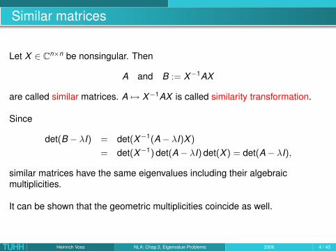
Let X ∈ Cn×n be nonsingular. Then
A and B := X−1AX
are called similar matrices. A 7→ X−1AX is called similarity transformation.
Since
det(B − λI) = det(X−1(A− λI)X )
= det(X−1) det(A− λI) det(X ) = det(A− λI),
similar matrices have the same eigenvalues including their algebraicmultiplicities.
It can be shown that the geometric multiplicities coincide as well.
TUHH Heinrich Voss NLA: Chap.3, Eigenvalue Problems 2006 4 / 43

Diagonalizable matrix
Let Ax j = λjx j , j = 1, . . . , k where λi 6= λj for i 6= j . Then the set {x1, . . . , xk}is linearly independent.
Let x =∑k
j=1 αjx j = 0. For j ∈ {1, . . . , k} it follows
(A− λ1I) · · · · · (A− λj−1I)(A− λj+1I) · · · · · (A− λk I)x = αj
k∏i=1,i 6=j
(λj − λi)x j = 0,
and therefore αj = 0.
In particular, if A has n different eigenvalues λj with eigenvectors x j , thenX := (x1, . . . , xn) is nonsingular, and it holds
AX = (Ax1, . . . , Axn) = (λ1x1, . . . , λnxn) = XΛ ⇐⇒ X−1AX = Λ
where Λ =: diag(λ1, . . . , λn) denotes a diagonal matrix with entries λ1, . . . , λn.
Hence, A is diagonalizable, i.e. similar to a diagonal matrix.
TUHH Heinrich Voss NLA: Chap.3, Eigenvalue Problems 2006 5 / 43

Diagonalizable matrix ct.
More generally, if for all eigenvalues λj , j = 1, . . . , k of A the algebraic andgeometric multiplies coincide (α(λj) = γ(λj)), then choosing in each of theeigenspaces Eλj a basis x j,1, . . . , x j,α(λj ), the matrix
X = (x1,1, . . . , x1,α(λ1), x2,1, . . . , xk,α(λk ))
is nonsingular, and it digonalizes A.
It can be shown that A is diagonalizable if and only if α(λj) = γ(λj) for everyeigenvalue λj of A.
For
A =
(0 10 0
)α(0) = 2 6= 1 = γ(0), and therefore not every matrix is diagonalizable.
TUHH Heinrich Voss NLA: Chap.3, Eigenvalue Problems 2006 6 / 43
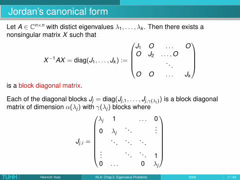
Jordan’s canonical formLet A ∈ Cn×n with distict eigenvalues λ1, . . . , λk . Then there exists anonsingular matrix X such that
X−1AX = diag(J1, . . . , Jk ) :=
J1 O . . . OO J2 . . . , O
. . .O O . . . Jk
is a block diagonal matrix.
Each of the diagonal blocks Jj = diag(Jj,1, . . . , Jj,γ(λj )) is a block diagonalmatrix of dimension α(λj) with γ(λj) blocks where
Jj,i =
λj 1 . . . 0
0 λj. . .
.... . . . . . . . .
.... . . . . . 1
0 . . . 0 λj
TUHH Heinrich Voss NLA: Chap.3, Eigenvalue Problems 2006 7 / 43
Hermitian matrices
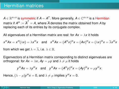
A ∈ Rn×n is symmetric if A = AT . More generally, A ∈ Cn×n is a Hermitianmatrix if AH := A
T= A, where A denotes the matrix obtained from A by
replacing each of its entries by its conjugate complex.
All eigenvalues of a Hermitian matrix are real: for Ax = λx it holds
xHAx = xH(λx) = λxHx and xHAx = (AHx)Hx = (Ax)Hx = (λx)Hx = λxHx
from which we get λ = λ, i.e. λ ∈ R.
Eigenvectors of a Hermitian matrix correponding to distinct eigenvalues areorthogonal: for Ax = λx , Ay = µy and λ 6= µ it holds
yHAx = λyHx and yHAx = (AHy)Hx = (Ay)Hx = µyHx .
Hence, (λ− µ)yHx = 0, and λ 6= µ implies yHx = 0.
TUHH Heinrich Voss NLA: Chap.3, Eigenvalue Problems 2006 8 / 43

Invariant subspace
A subspace V of Cn is an invariant subspace of A if Ax ∈ V for every x ∈ V .
Every invariant subspace of A contains an eigenvector of A.
Let x1, . . . , xk ∈ Cn be a basis of V . Then for j = 1, . . . , k there exists bij ∈ Csuch that Ax j =
∑ki=1 bijx i .
Let λ be an eigenvalue of B = (bij) ∈ Ck×k with eigenvector ξ = (ξ1, . . . , ξk )T ,and let x :=
∑ki=1 ξix i 6= 0. Then
Ax =k∑
j=1
ξjAx j =k∑
j=1
k∑i=1
ξjbijx i =k∑
i=1
(k∑
j=1
bijξj)x i =k∑
i=1
λξix i = λx .
TUHH Heinrich Voss NLA: Chap.3, Eigenvalue Problems 2006 9 / 43

Hermitian matrices are diagonalizable
Let A be a Hermitian matrix. Then there exists a unitary matrix U ∈ Cn×n (i.e.UHU = I) such that
UHAU = diag(λ1, . . . , λn).
Let x1 be an eigenvector of A such that Ax1 = λ1x1 and (x1)Hx1 = 1. Thenfor x ∈ Cn such that xHx1 = 0 it holds
(Ax)Hx1 = xHAHx1 = xH(Ax1) = λ1xHx1 = 0.
Hence, V1 := {x ∈ Cn : xHx1 = 0} is an invariant subspace of A, andtherefore it contains an eigenvector x2 which can be normalized such that(x2)Hx2 = 1.If x1, . . . , x j are j orthogonal eigenvectors of A, then in the same way as before
Vj := {x1, . . . , x j}⊥ = {x ∈ Cn : xHx i = 0, i = 1, . . . , j}
is an invariant subspace of A, and hence there exists an eigenvector x j+1
which is orthogonal to x1, . . . , x j .U = (x1, . . . , xn) renders the desired property.
TUHH Heinrich Voss NLA: Chap.3, Eigenvalue Problems 2006 10 / 43

Rayleigh’s principle
Let A ∈ Cn×n be a Hermitian matrix. Then for x 6= 0
RA(x) :=xHAxxHx
is called Rayleigh quotient of A at x .
Let λ1 ≤ λ2 ≤ · · · ≤ λn be the eigenvalues of A, and let x1, . . . , xn be a set ofcorresponding orthogonalized eigenvectors. Then it holds
λ1 = minx 6=0
RA(x) and λn = maxx 6=0
RA(x).
for i = 1, 2, . . . , n it holds
λi = min{RA(x) : x ∈ Cn, xHx j = 0, j = 1, . . . , i − 1}= max{RA(x) : x ∈ Cn, xHx j = 0, j = i + 1, . . . , n}
TUHH Heinrich Voss NLA: Chap.3, Eigenvalue Problems 2006 11 / 43

Proof of Rayleigh’s principle
Let x1, . . . , xn be an orthonormal system of eigenvectors of A ∈ Cn×n whereAx j = λjx j .
For x ∈ Cn, x 6= 0 let x =∑n
j=1 ξjx j .
xHx =( n∑
j=1
ξjx j)H( n∑
k=1
ξk xk)
=n∑
j,k=1
ξjξk (x j)Hxk =n∑
j=1
|ξj |2
xHAx =( n∑
j=1
ξjx j)H
A( n∑
k=1
ξk xk)
=( n∑
j=1
ξjx j)H( n∑
k=1
ξk Axk)
=( n∑
j=1
ξjx j)H( n∑
k=1
ξkλk xk)
=n∑
j=1
λj |ξj |2
Hence,
RA(x) =n∑
j=1
αjλj , with αj =|ξj |2∑n
k=1 |ξk |2
TUHH Heinrich Voss NLA: Chap.3, Eigenvalue Problems 2006 12 / 43
Proof of Rayleigh’s principle
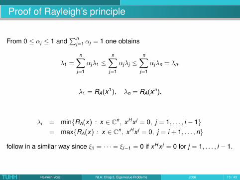
From 0 ≤ αj ≤ 1 and∑n
j=1 αj = 1 one obtains
λ1 =n∑
j=1
αjλ1 ≤n∑
j=1
αjλj ≤n∑
j=1
αjλn = λn.
λ1 = RA(x1), λn = RA(xn).
λi = min{RA(x) : x ∈ Cn, xHx j = 0, j = 1, . . . , i − 1}= max{RA(x) : x ∈ Cn, xHx j = 0, j = i + 1, . . . , n}
follow in a similar way since ξ1 = · · · = ξi−1 = 0 if xHx j = 0 for j = 1, . . . , i − 1.
TUHH Heinrich Voss NLA: Chap.3, Eigenvalue Problems 2006 13 / 43

Numerical methods
Linear systems of equations Ax = b can be solved by a finite algorithm (i.e. afinite number of operations) like Gauss elimination.
Determining an eigenvalue of a matrix A ∈ Rn×n is equivalent to finding a rootof the characteristic polynomial
χ(λ) := det(A− λI) = 0.
It is known (Theorem of Abel) that for n ≥ 5 there is no formula for solving
det(A− λI) = 0
for λ. Hence, the eigenvalue problem Ax = λx usually can be solved only byiterative methods.
TUHH Heinrich Voss NLA: Chap.3, Eigenvalue Problems 2006 14 / 43

Example
A =
0.2 0.3 0.40.6 0.2 0.50.2 0.5 0.1
Choose any vector x0 ∈ R3 and compute the sequence
xk := Axk−1, k = 1, 2, 3, . . .
After a small number of steps (≈ 10) we obtain
xk =
0.51220.69740.5013
and ‖Axk − xk‖ small.
xk seems to be an eigenvector corresponding to the eigenvalue λ = 1.Is this a miracle?
TUHH Heinrich Voss NLA: Chap.3, Eigenvalue Problems 2006 15 / 43

A is stochastic
All elements of A are nonnegative, and every column of A adds to 1. Matriceswith these properties are called stochastic. They describe the behavior ofMarkov chaines.
If A is stochastic, then every row of AT adds to 1, and therefore (1, 1, . . . , 1)T
is an eigenvector of AT corresponding to the eigenvalue 1.
det(A− λI) = det(AT − λI)
implies that the eigenvalues of A and AT coincide. Hence, every stochasticmatrix has one eigenvalue λ = 1.
TUHH Heinrich Voss NLA: Chap.3, Eigenvalue Problems 2006 16 / 43

Power method
Assume that A is diagonizable, i.e. there exist n linearly independenteigenvectors u1, . . . , un of A, and assume that λ1 is a dominant eigenvalue
|λ1| > |λ2|, |λ3|, . . . , |λn|.
The initial vector x0 can be representeted as
x0 =n∑
j=1
αjuj
Ax0 = A( n∑
j=1
αjuj)
=n∑
j=1
αjAuj =n∑
j=1
αjλjuj
TUHH Heinrich Voss NLA: Chap.3, Eigenvalue Problems 2006 17 / 43
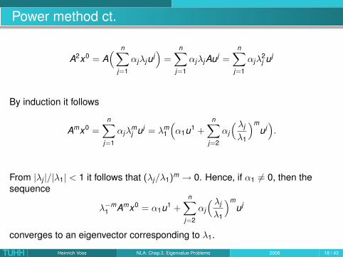
Power method ct.
A2x0 = A( n∑
j=1
αjλjuj)
=n∑
j=1
αjλjAuj =n∑
j=1
αjλ2j uj
By induction it follows
Amx0 =n∑
j=1
αjλmj uj = λm
1
(α1u1 +
n∑j=2
αj
( λj
λ1
)muj
).
From |λj |/|λ1| < 1 it follows that (λj/λ1)m → 0. Hence, if α1 6= 0, then the
sequence
λ−m1 Amx0 = α1u1 +
n∑j=2
αj
( λj
λ1
)muj
converges to an eigenvector corresponding to λ1.
TUHH Heinrich Voss NLA: Chap.3, Eigenvalue Problems 2006 18 / 43
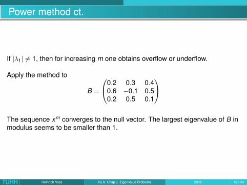
Power method ct.
If |λ1| 6= 1, then for increasing m one obtains overflow or underflow.
Apply the method to
B =
0.2 0.3 0.40.6 −0.1 0.50.2 0.5 0.1
The sequence xm converges to the null vector. The largest eigenvalue of B inmodulus seems to be smaller than 1.
TUHH Heinrich Voss NLA: Chap.3, Eigenvalue Problems 2006 19 / 43
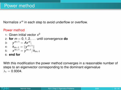
Power method
Normalize xm in each step to avoid underflow or overflow.
Power method1: Given initial vector x0
2: for m = 0, 1, 2, . . . until convergence do3: ym+1 = Axm;4: km+1 = ‖ym+1‖5: xm+1 = ym+1/km+16: end for
With this modification the power method converges in a reasonable number ofsteps to an eigenvector corresponding to the dominant eigenvalueλ1 = 0.9304.
TUHH Heinrich Voss NLA: Chap.3, Eigenvalue Problems 2006 20 / 43
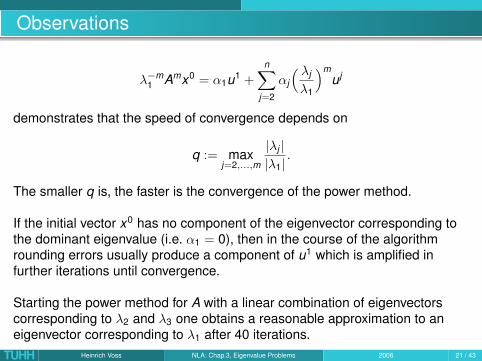
Observations
λ−m1 Amx0 = α1u1 +
n∑j=2
αj
( λj
λ1
)muj
demonstrates that the speed of convergence depends on
q := maxj=2,...,m
|λj ||λ1|
.
The smaller q is, the faster is the convergence of the power method.
If the initial vector x0 has no component of the eigenvector corresponding tothe dominant eigenvalue (i.e. α1 = 0), then in the course of the algorithmrounding errors usually produce a component of u1 which is amplified infurther iterations until convergence.
Starting the power method for A with a linear combination of eigenvectorscorresponding to λ2 and λ3 one obtains a reasonable approximation to aneigenvector corresponding to λ1 after 40 iterations.
TUHH Heinrich Voss NLA: Chap.3, Eigenvalue Problems 2006 21 / 43
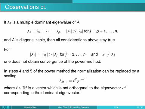
Observations ct.
If λ1 is a multiple dominant eigenvalue of A
λ1 = λ2 = · · · = λp, |λ1| > |λj | for j = p + 1, . . . , n,
and A is diagonalizable, then all considerations above stay true.
For|λ1| = |λ2| > |λj | for j = 3, . . . , n, and λ1 6= λ2
one does not obtain convergence of the power method.
In steps 4 and 5 of the power method the normalization can be replaced by ascaling
km+1 = `T ym+1
where ` ∈ Rn is a vector which is not orthogonal to the eigenvector u1
corresponding to the dominant eigenvector.
TUHH Heinrich Voss NLA: Chap.3, Eigenvalue Problems 2006 22 / 43

Inverse iteration
Applying the power method to the inverse matrix A−1 one can determine thesmallest eigenvalue in modulus.
Inverse iterationGiven initial vector x0
for m = 0, 1, 2, . . . until convergence doSolve Aym+1 = xm for ym+1
km+1 = ‖ym+1‖xm+1 = ym+1/km+1
end for
Applying inverse iteration to the matrix B one gets fast convergence to aneigenvector corresponding to the smallest eigenvalue λ3 = −0.2111. For Athe convergence is very slow. What is the difference?
TUHH Heinrich Voss NLA: Chap.3, Eigenvalue Problems 2006 23 / 43
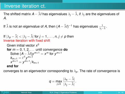
Inverse iteration ct.The shifted matrix A− λI has eigenvalues λj − λ, if λj are the eigenvalues ofA.
If λ is not an eigenvalue of A, then (A− λI)−1 has eigenvalues 1λj−λ
.
If |λp − λ| < |λj − λ| for j = 1, . . . , n, j 6= p thenInverse iteration with fixed shift
Given initial vector x0
for m = 0, 1, 2, . . . until convergence doSolve (A− λI)ym+1 = xm for ym+1
km+1 = `T ym+1
xm+1 = ym+1/km+1end for
converges to an eigenvector corresponding to λp. The rate of convergence is
q = maxj 6=k
|λk − λ||λj − λ|
.
TUHH Heinrich Voss NLA: Chap.3, Eigenvalue Problems 2006 24 / 43

Inverse iteration with variable shiftsFor large m it holds that xm is an approximate eigenvector corresponding toλp and `T xm = 1. Hence,
km+1 = `T ym+1 = `T ((A− λI)−1xm) ≈ 1λp − λ
`T xm =1
λp − λ.
This observations suggests to iterate the shift as well:
km+1 ≈1
λm+1 − λm=⇒ λm+1 := λm + 1/km+1
Inverse iteration with variable shiftsGiven initial vector x0 and initial approximation λ0for m = 0, 1, 2, . . . until convergence do
Solve (A− λmI)ym+1 = xm for ym+1
km+1 = `T ym+1
xm+1 = ym+1/km+1λm+1 = λm + 1/km+1
end forTUHH Heinrich Voss NLA: Chap.3, Eigenvalue Problems 2006 25 / 43

Quadratic convergence
Let λ be an algebraically simple eigenvalue of A (i.e. λ is a simple root ofdet(A− λI) = 0), let u be a corresponding eigenvector such that `T u = 1.
Then inverse iteration with variable shifts converges locally and quadraticallyto (λ, u): There exists some positive constant C > 0 such that, if λ0 issufficiently close to λ and x0 is sufficiently close to u, then it holds
|λ− λm+1| ≤ C|λ− λm|2 and ‖u − xm+1‖ ≤ C‖u − xm‖2.
TUHH Heinrich Voss NLA: Chap.3, Eigenvalue Problems 2006 26 / 43
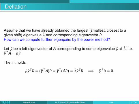
Deflation
Assume that we have already obtained the largest (smallest, closest to agiven shift) eigenvalue λ and corresponding eigenvector u.How can we compute further eigenpairs by the power method?
Let y be a left eigenvector of A corresponding to some eigenvalue µ 6= λ, i.e.yT A = µy .
Then it holds
µyT u = (yT A)u = yT (Au) = λyT u =⇒ yT u = 0.
TUHH Heinrich Voss NLA: Chap.3, Eigenvalue Problems 2006 27 / 43
Deflation ct.
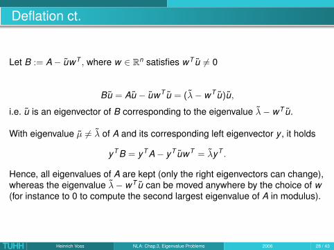
Let B := A− uwT , where w ∈ Rn satisfies wT u 6= 0
Bu = Au − uwT u = (λ− wT u)u,
i.e. u is an eigenvector of B corresponding to the eigenvalue λ− wT u.
With eigenvalue µ 6= λ of A and its corresponding left eigenvector y , it holds
yT B = yT A− yT uwT = λyT .
Hence, all eigenvalues of A are kept (only the right eigenvectors can change),whereas the eigenvalue λ− wT u can be moved anywhere by the choice of w(for instance to 0 to compute the second largest eigenvalue of A in modulus).
TUHH Heinrich Voss NLA: Chap.3, Eigenvalue Problems 2006 28 / 43
Symmetric matrices
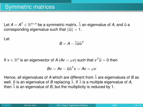
Let A = AT ∈ Rn×n be a symmetric matrix, λ an eigenvalue of A, and u acorresponding eigenvalue such that ‖u‖ = 1.
LetB = A− λuuT
If v ∈ Rn is an eigenvector of A (Av = µv ) such that vT u = 0 then
Bv = Av − uuT v = Av = µv
Hence, all eigenvalues of A which are different from λ are eigenvalues of B aswell. 0 is an eigenvalue of B replacing λ. If λ is a multiple eigenvalue of A,then λ is an eigenvalue of B, but the multiplicity is reduced by 1.
TUHH Heinrich Voss NLA: Chap.3, Eigenvalue Problems 2006 29 / 43
QR Algorithm
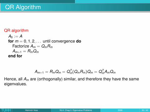
QR algorithmA0 := Afor m = 0, 1, 2, . . . until convergence do
Factorize Am = QmRmAm+1 = RmQm
end for
Am+1 = RmQm = QTm(QmRm)Qm = QT
mAmQm
Hence, all Am are (orthogonally) similar, and therefore they have the sameeigenvalues.
TUHH Heinrich Voss NLA: Chap.3, Eigenvalue Problems 2006 30 / 43

QR algorithm ct.
If the eigenvalues of A are pairwise different of each other in modulus,
|λ1| > |λ2 > | · · · > |λn|
and if a further technical condition is satisfied, then the QR algorithmconverges in the following sense:
If (Am)jk = a(m)jk , then
limm→∞
a(m)jk = 0 for j > k
limm→∞
a(m)jj = λj for j = 1, . . . , n
TUHH Heinrich Voss NLA: Chap.3, Eigenvalue Problems 2006 31 / 43
QR algorithm and power method
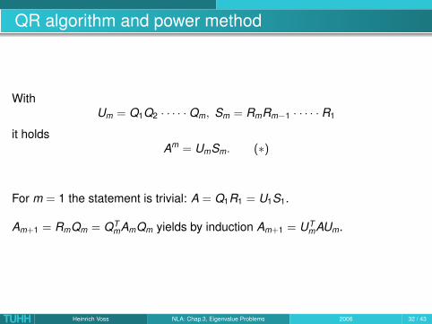
WithUm = Q1Q2 · · · · ·Qm, Sm = RmRm−1 · · · · · R1
it holdsAm = UmSm. (∗)
For m = 1 the statement is trivial: A = Q1R1 = U1S1.
Am+1 = RmQm = QTmAmQm yields by induction Am+1 = UT
mAUm.
TUHH Heinrich Voss NLA: Chap.3, Eigenvalue Problems 2006 32 / 43

QR algorithm and power method ct.If (∗) is valid for some m − 1, then it follows from the definition of Am+1
Rm = Am+1QTm = UT
mAUmQTm = UT
mAUm−1
Multiplying by Sm−1 from the right und by Um from the left we obtain
UmSm = AUm−1Sm−1 = Am
which is the proposition for m.
From (∗) we obtain for the first unit vector e1 and ρ = (Rm)(1,1)
Ane1 = UmRme1 = ρUme1.
Hence, the first column has the same direction as the m-th iterate of thepower method with initial vector e1, and it is not surprising that r11 convergesto the largest eigenvalue of A in modulus and the first column to acorresponding eigenvector.
TUHH Heinrich Voss NLA: Chap.3, Eigenvalue Problems 2006 33 / 43

Examples
For
A =
1 −1 −14 6 3−4 −4 −1
the upper triangular form appears after approximately 10 steps, and thediagonal elements are in the right order.
For
B =
1 0 12 3 −1−2 −2 2
the upper triangular form is arrived after approximately 20 steps, but thediagonal elements are not ordered by magnitude (So, the technical conditionof the last Theorem is not satisfied).After further 50 steps the diagonal elements are ordered by magnitude.
TUHH Heinrich Voss NLA: Chap.3, Eigenvalue Problems 2006 34 / 43
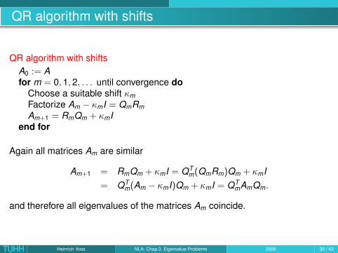
QR algorithm with shifts
QR algorithm with shiftsA0 := Afor m = 0, 1, 2, . . . until convergence do
Choose a suitable shift κmFactorize Am − κmI = QmRmAm+1 = RmQm + κmI
end for
Again all matrices Am are similar
Am+1 = RmQm + κmI = QTm(QmRm)Qm + κmI
= QTm(Am − κmI)Qm + κmI = QT
mAmQm.
and therefore all eigenvalues of the matrices Am coincide.
TUHH Heinrich Voss NLA: Chap.3, Eigenvalue Problems 2006 35 / 43

Choice of shifts
Let Qj and Rj be the orthogonal and upper triangular matrices obtained in theQR algorithm with shifts κj , and let
Um = Q1Q2 · · · · ·Qm, Sm = RmRm−1 · · · · · R1.
ThenUmSm = (A− κmI)(A− κm−1I) · · · · · (A− κ1I). (+)
From Am+1 = QTmAmQm it follows immediately by induction Am+1 = UH
mAUm.
For m = 1 equation (+) reads
U1S1 = Q1R1 = A− κ1I
which is the decomposition in the first step of the QR algorithm with shifts.
TUHH Heinrich Voss NLA: Chap.3, Eigenvalue Problems 2006 36 / 43

Choice of shifts ct.
Assume that (+) holds for some m − 1. From the definition of Am+1 follows
Rm = (Am+1 − κmI)QTm = UT
m(A− κmI)UmQTm = UT
m(A− κmI)Um−1.
Multiplying with Sm−1 from the right and Um from the left one obtains
UmSm = (A− κmI)Um−1Sm−1 = (A− κmI)(A− κm−1I) · · · · · (A− κ1I).
TUHH Heinrich Voss NLA: Chap.3, Eigenvalue Problems 2006 37 / 43
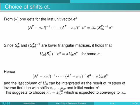
Choice of shifts ct.
From (+) one gets for the last unit vector en
(AT − κmI)−1 · · · · · (AT − κ1I)−1en = Um(STm)−1en
Since STm and (ST
m)−1 are lower triangular matrices, it holds that
Um(STm)−1en = σUmen for some σ.
Hence(AT − κmI)−1 · · · · · (AT − κ1I)−1en = σUmen
and the last column of Um can be interpreted as the result of m steps ofinverse iteration with shifts κ1,. . . ,κm and initial vector en
This suggests to choose κm = a(m)n,n which is expected to converge to λn.
TUHH Heinrich Voss NLA: Chap.3, Eigenvalue Problems 2006 38 / 43

Reducing the cost
The most expensive part in the QR algorithm (shifted or not) is thecomputation of the QR factorization in every step.
This cost can be reduced considerably, if the matrix is transformed to upperHessenberg form first:
A =
a11 a12 a13 . . . a1,n−1 a1na21 a22 a23 . . . a2,n−1 a2n0 a32 a33 . . . a3,n−1 a3n...
. . . . . ....
. . . . . .0 0 0 . . . an.n−1 ann
A has upper Hessenberg form, if ajk = 0 for j > k1.
TUHH Heinrich Voss NLA: Chap.3, Eigenvalue Problems 2006 39 / 43
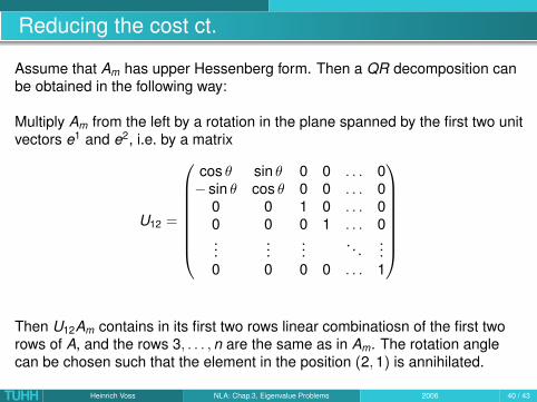
Reducing the cost ct.
Assume that Am has upper Hessenberg form. Then a QR decomposition canbe obtained in the following way:
Multiply Am from the left by a rotation in the plane spanned by the first two unitvectors e1 and e2, i.e. by a matrix
U12 =
cos θ sin θ 0 0 . . . 0− sin θ cos θ 0 0 . . . 0
0 0 1 0 . . . 00 0 0 1 . . . 0...
......
. . ....
0 0 0 0 . . . 1
Then U12Am contains in its first two rows linear combinatiosn of the first tworows of A, and the rows 3, . . . , n are the same as in Am. The rotation anglecan be chosen such that the element in the position (2, 1) is annihilated.
TUHH Heinrich Voss NLA: Chap.3, Eigenvalue Problems 2006 40 / 43

Reducing the cost ct.
Multiplying U12Am from the left by a rotation matrix U23 corresponding to rows2 and 3, we annihilate the element in position (3, 2), which does not changethe element 0 in the (2, 1) position.
Continuing that way we annihilate the elements in positions (i + 1, 1) by arotation Ui,i+1 in the plane spanned by ei and ei+1.
We finally arrive at
Un−1,n · . . . · · ·U23U12Am = R, i.e. Am = QR, Q = UT12 · · · · · UT
n−1,n.
TUHH Heinrich Voss NLA: Chap.3, Eigenvalue Problems 2006 41 / 43

Reducing the cost ct.
Am+1 = RQ = RUT12 · · · · · UT
n−1,n
Multiplying R by UT12 combines the first two columns of R and leaves the other
columns unchanged. Multiplying by UT23 combines columns 2 and 3 and
leaves the other ones unchanged, etc.
ObviouslyAm+1 = RUT
12 · · · · · UTn−1,n
becomes an upper Hessenberg matrix.
TUHH Heinrich Voss NLA: Chap.3, Eigenvalue Problems 2006 42 / 43

Reduction to Hessenberg form
A given matrix can be transformed to upper Hessenberg form usingHouseholder matrices.For
A =
(a11 cT
b B
), B ∈ R(n−1)×(n−1), b, c ∈ Rn−1
let w ∈ Rn−1, ‖w‖ = 1 such that the Householder matrix Q1 = I − 2wwT mapsb to a multiple of the first unit vector in Rn−1.
Then with P1 =
(1 00 Q1
)we get
A1 := P1AP1 =
a11 cT Q1k0...0
Q1BQ1
and the first column already has obtained the desired form.The following columns can be tranformed in a similar way.
TUHH Heinrich Voss NLA: Chap.3, Eigenvalue Problems 2006 43 / 43