numerical methods for conservation laws and related...
TRANSCRIPT
Numerical methods for conservation laws
and related equations
Siddhartha Mishra

About these notes
These notes present numerical methods for conservation laws and related time-dependent nonlinear partial differential equations. The focus is on both simplescalar problems as well as multi-dimensional systems.
The MATLAB package Compack (Conservation Law MATLAB Package) hasbeen developed as an educational tool to be used with these notes. All the numericalexperiments in the lecture notes have been done in Compack. The scripts used togenerate figures and tables are all in the +Notes sub-package. For instance, to gen-erate the plots in Figure 2.3, run Notes.Chapter2.central() from the Compackbase folder. Figures are saved to the output folder. Compack can be downloadedfrom http://www.sam.math.ethz.ch/~ulrikf/compack.zip.
iii

Contents
About these notes iii
Chapter 1. Introduction 11.1. Examples for conservation laws. 21.2. Content and scope of these notes 5
Chapter 2. Linear Transport Equations 72.1. Method of characteristics 72.2. Finite difference schemes for the transport equation 92.3. An upwind scheme 122.4. Stability for the upwind scheme 14
Chapter 3. Scalar conservation laws 173.1. Characteristics for Burger’s equation 193.2. Weak solutions 213.3. Entropy solutions 27
Chapter 4. Finite volume schemes for scalar conservation laws 334.1. Finite volume scheme 334.2. Approximate Riemann Solvers 394.3. Comparison of different finite volume schemes 444.4. Convergence Analysis 454.5. A note on boundary conditions 54
Chapter 5. Second-order (high-resolution)finite volume schemes 57
5.1. Order of accuracy 595.2. The REA algorithm 635.3. The minmod limiter 675.4. Other limiters 705.5. Flux limiters and the TVD property. 725.6. High-resolution methods for nonlinear problems. 735.7. Second-order semi-discrete schemes. 755.8. Time stepping 765.9. High-resolution algorithm 775.10. Numerical experiments 77
Chapter 6. Linear hyperbolic systems in one space dimension 816.1. Examples for linear systems 816.2. Hyperbolicity and characteristic decomposition 836.3. Solutions of Riemann problems, waves 84
v
vi CONTENTS
6.4. Finite volume schemes 856.5. Numerical experiments 886.6. High-order finite volume schemes 916.7. Numerical experiments 93
Appendix A. Results from real analysis 95
Bibliography 97
CHAPTER 1
Introduction
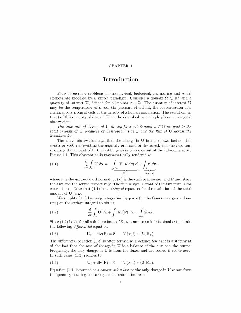
Many interesting problems in the physical, biological, engineering and socialsciences are modeled by a simple paradigm: Consider a domain Ω ⊂ Rn and aquantity of interest U, defined for all points x ∈ Ω. The quantity of interest Umay be the temperature of a rod, the pressure of a fluid, the concentration of achemical or a group of cells or the density of a human population. The evolution (intime) of this quantity of interest U can be described by a simple phenomenologicalobservation:
The time rate of change of U in any fixed sub-domain ω ⊂ Ω is equal to thetotal amount of U produced or destroyed inside ω and the flux of U across theboundary ∂ω.
The above observation says that the change in U is due to two factors: thesource or sink, representing the quantity produced or destroyed, and the flux, rep-resenting the amount of U that either goes in or comes out of the sub-domain, seeFigure 1.1. This observation is mathematically rendered as
(1.1)d
dt
∫ω
U dx = −∫∂ω
F · ν dσ(x)︸ ︷︷ ︸flux
+
∫ω
S dx︸ ︷︷ ︸source
,
where ν is the unit outward normal, dσ(x) is the surface measure, and F and S arethe flux and the source respectively. The minus sign in front of the flux term is forconvenience. Note that (1.1) is an integral equation for the evolution of the totalamount of U in ω.
We simplify (1.1) by using integration by parts (or the Gauss divergence theo-rem) on the surface integral to obtain
(1.2)d
dt
∫ω
U dx +
∫ω
div(F) dx =
∫ω
S dx.
Since (1.2) holds for all sub-domains ω of Ω, we can use an infinitesimal ω to obtainthe following differential equation:
(1.3) Ut + div(F) = S ∀ (x, t) ∈ (Ω,R+).
The differential equation (1.3) is often termed as a balance law as it is a statementof the fact that the rate of change in U is a balance of the flux and the source.Frequently, the only change in U is from the fluxes and the source is set to zero.In such cases, (1.3) reduces to
(1.4) Ut + div(F) = 0 ∀ (x, t) ∈ (Ω,R+).
Equation (1.4) is termed as a conservation law, as the only change in U comes fromthe quantity entering or leaving the domain of interest.
1
2 1. INTRODUCTION
Ω
Ωδ
Figure 1.1. An illustration of conservation in a domain with thechange being determined by the net flux.
The discussion so far is very general. We have not yet specified the explicitforms of U,F and S. In fact, the conservation law (1.4) and the balance law (1.3) aregeneric to a very large number of models. Explicit forms of the quantity of interest,flux and source depend on the specific model being considered. The modeling ofthe flux F is the core function of a physicist, biologist, engineer or other domainscientists. We will provides several examples to illustrate conservation laws.
1.1. Examples for conservation laws.
For simplicity of the exposition, we begin with scalar examples, i.e, the quantityof interest U is a scalar U .
Scalar transport equation. Let U = U denote the concentration of a chemi-cal (for example, a pollutant in a river). Assume that the river flows with a velocityfield a(x, t) and we know the velocity field at all points in the river. The pollutantwill clearly be transported in the direction of the velocity and so the flux in thiscase is F = aU . Since there is no production or destruction of the pollutant duringthe flow, the source term in (1.3) is set to zero. Consequently, the conservation law(1.4) takes the form
(1.5) Ut + div(a(x, t)U) = 0.
This equation is linear. In the simple case of one space dimension and a constantvelocity field a(x, t) ≡ a, (1.5) reduces to
(1.6) Ut + aUx = 0.
The scalar one-dimensional equation (1.6) is often referred to as the transport oradvection equation.
The heat equation. Another illustrative example of a conservation law isprovided by heat conduction. Assume that a hot material (like a metal block) isheated at one end and is left to cool afterwards, without providing any additionalsource of heat. It is a common observation that the heat spreads or diffuses out
1.1. EXAMPLES FOR CONSERVATION LAWS. 3
and the temperature of the material becomes uniform after some time. Let U bethe temperature of the material. Diffusion of heat is governed by Fourier’s or Fick’slaw
F(U) = −k∇U.
Here, k is the conductivity tensor for the medium. The minus sign is due to thefact that heat flows from hotter to cooler zones. Substituting Fourier’s law into theconservation law (1.4), we obtain the heat equation
(1.7) Ut − div(k∇U) = 0.
If the conductivity is assumed to be unity and the material is one-dimensional (likea rod), (1.7) reduces to the well-known one-dimensional heat equation
(1.8) Ut − Uxx = 0.
The scalar transport equation (1.5) and the heat equation (1.7) are both linearequations and deal with the evolution of a single scalar quantity. As nature is toocomplicated to be described by scalar linear equations, their utility is limited. Next,we present a nonlinear system of conservation laws.
Euler equations of gas dynamics. A gas (as an example consider air) con-sists of a large number of molecules. The motion of each molecule can be trackedindividually. This description is termed as the particle description and leads toa very large number of ODEs. The resulting system of ODEs is too large to becomputationally feasible. Instead, a more macroscopic description is used. In amacroscopic model, the key variables of interest are: the density ρ, the velocityfield u and the gas pressure p. All these quantities can be measured experimen-tally. The relevant conservation laws are
• Conservation of mass: It is well-known in fluid dynamics that the totalmass of the gas is conserved. Mathematically, using Kelvin’s theorem,this translates into
ρt + div(ρu) = 0.
• Conservation of momentum: By Newton’s second law of motion, the rateof change of momentum equals force. In the absence of external forces, thegas pressure is the only force acting on the gas. The resulting conservationlaw is
(ρu)t + div(ρu⊗ u) +∇p = 0.
Note that the above conservation laws implies that the rate of change ofthe advective (material) derivative of the momentum equals the gradientof pressure. This is a consequence of the following observation: Gas flowsfrom high to low pressure.
The symbol ⊗ is the tensor product, i.e, for any two vectors a =(a1, a2, a3) and b = (b1, b2, b3), we have
a⊗ b =
a1b1 a1b2 a1b3a2b1 a2b2 a2b3a3b1 a3b2 a3b3
.
4 1. INTRODUCTION
• Conservation of energy: The total energy of a gas is a sum of its kineticand internal (potential) energy. The kinetic energy has the standard ex-pression
Ek =1
2ρ|u|2,
whereas the internal energy is determined by an equation of state. If thegas is an ideal gas, then the equation of state is
Ei =p
γ − 1,
where γ is the gas constant. It takes the values 5/3 and 7/5 for mono-atomic and diatomic gases, respectively. Hence, the total energy of anideal gas is
(1.9) E =p
γ − 1+
1
2ρ|u|2.
The rate of change of total energy is computed as:
Et + div((E + p)u) = 0.
All the three conservation laws are combined together and written in divergenceform to obtain the Euler equations of gas dynamics:
(1.10)
ρt + div(ρu) = 0,
(ρu)t + div(ρu⊗ u + pI) = 0,
Et + div((E + p)u) = 0,
where I denotes the 3 × 3 identity matrix. The above system is an example ofa multi-dimensional nonlinear system of conservation laws. This derivation of theEuler equations was very brief and details can be found in fluid dynamics textbookslike [7]. We ignore fluid viscosity effects and heat conduction in the gas whilederiving (1.10).
The above examples already reveal a multitude of diverse physical phenomenathat can be modeled in terms of conservation laws. The flux F in (1.4) is often afunction of U and its derivatives,
F = F(U,∇U,∇2U, . . . )
For simplicity of the analysis, it is common to neglect the role of the higher thanfirst-order derivatives. Hence, the flux is of the form:
F = F(U,∇U).
If it is of the form F = F(U), then the conservation law (1.4) is a first-order PDE.It is usually classified as hyperbolic. The notion of hyperbolicity will be describedin detail in the sequel. The scalar transport equation (1.5) and the Euler equationsof gas dynamics (1.10) are examples for hyperbolic equations.
If we have F = F(∇U), then the conservation law (1.4) is a second-orderPDE and is often classified as parabolic. The heat equation (1.7) is an exampleof a parabolic equation. When the flux F depends on both the function U andits first derivative, the conservation law (1.4) is termed as a convection-diffusionequation. In these notes, we will consider hyperbolic equations and convection-diffusion equations with the convection dominating the diffusion.
1.2. CONTENT AND SCOPE OF THESE NOTES 5
1.1.1. Other examples. Examples for conservation laws of both the hyper-bolic and convection-diffusion type abound in nature. In these notes, we will con-sider the scalar Burgers equation, the Buckley-Leverett equation (modeling flowsin oil and gas reservoirs), the wave equation, the shallow water equations of me-teorology and oceanography, the equations for linear and nonlinear elastic wavesthat arise in materials science and the equations of magnetohydrodynamics (MHD)from plasma physics.
1.2. Content and scope of these notes
The reason for studying conservation laws extensively is obvious: They arise inmany models in the sciences, ranging from the design of aircraft (Euler equations)to the study of supernovas in astrophysics (MHD equations). Since interestingconservation laws like the Euler equations are nonlinear, it is not possible to obtainexplicit solution formulas. Hence, numerical methods need to be developed forapproximating or simulating the solutions of conservation laws. The design andimplementation of efficient numerical methods is the main focus of these notes.
In order to design efficient numerical methods, we need to understand theanalytical structure of the solutions of conservation laws. Therefore, we will brieflydiscuss theoretical properties of the solutions that are relevant for the design andanalysis of numerical schemes.
We begin with the study of one-dimensional scalar problems. Both linear andnonlinear equations are considered, and efficient numerical schemes are describedfor them. Then, the focus shifts to linear and nonlinear systems like the Eulerequations of gas dynamics. Finally, we consider the multi-dimensional versions ofsystems of conservation laws and describe efficient numerical schemes for them.

CHAPTER 2
Linear Transport Equations
In this chapter we consider the one-dimensional version of the linear transportequation,
(2.1) Ut + a(x, t)Ux = 0 ∀ (x, t) ∈ R× R+.
The simplest case of the scalar transport equation arises when the velocity field isconstant, that is, a(x, t) ≡ a. The resulting transport equation is
(2.2) Ut + aUx = 0.
The rather simple equation (2.2) has served as a crucible for designing highly effi-cient schemes for much more complicated systems of equations. We concentrate onit for the rest of this chapter.
2.1. Method of characteristics
The initial value problem (or Cauchy problem) for (2.1) consists of finding asolution of (2.1) that also satisfies the initial condition
(2.3) U(x, 0) = U0(x) ∀ x ∈ R.
It is well known that the solution of the initial value problem can be constructed byusing the method of characteristics. The idea underlying this method is to reduce aPDE like (2.1) to an ODE by utilizing the structure of the solutions. As an ansatz,assume that we are given some curve x(t), along which the solution U is constant.This means that
0 =d
dtU(x(t), t) (as U is constant along x(t))
= Ut(x(t), t) + Ux(x(t), t)x′(t) (chain rule).
We also know that Ut(x(t), t) + Ux(x(t), t)a(x(t), t) = 0, since U is assumed to bea solution of (2.1). Therefore, if x(t) satisfies the ODE
(2.4)x′(t) = a(x(t), t)
x(0) = x0,
then x(t) is precisely such a curve. The solution x(t) of this equation is calleda characteristic curve. From ODE theory, we know that solutions of (2.4) existprovided that a is Lipschitz continuous in both arguments. It may or may not bepossible to find an explicit solution formula for (2.4).
The importance of characteristic curves lies in the property that U is constantalong them:
U(x(t), t) = U(x(0), 0) = U0(x0).
7
8 2. LINEAR TRANSPORT EQUATIONS
X0
X( t)
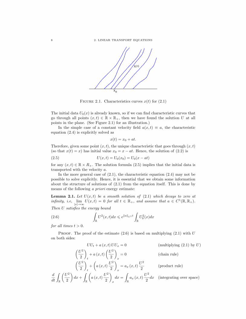
Figure 2.1. Characteristics curves x(t) for (2.1)
The initial data U0(x) is already known, so if we can find characteristic curves thatgo through all points (x, t) ∈ R × R+, then we have found the solution U at allpoints in the plane. (See Figure 2.1) for an illustration.)
In the simple case of a constant velocity field a(x, t) ≡ a, the characteristicequation (2.4) is explicitly solved as
x(t) = x0 + at.
Therefore, given some point (x, t), the unique characteristic that goes through (x, t)(so that x(t) = x) has initial value x0 = x− at. Hence, the solution of (2.2) is
(2.5) U(x, t) = U0(x0) = U0(x− at)
for any (x, t) ∈ R×R+. The solution formula (2.5) implies that the initial data istransported with the velocity a.
In the more general case of (2.1), the characteristic equation (2.4) may not bepossible to solve explicitly. Hence, it is essential that we obtain some informationabout the structure of solutions of (2.1) from the equation itself. This is done bymeans of the following a priori energy estimate:
Lemma 2.1. Let U(x, t) be a smooth solution of (2.1) which decays to zero atinfinity, i.e, lim
|x|→∞U(x, t) = 0 for all t ∈ R+, and assume that a ∈ C1(R,R+).
Then U satisfies the energy bound
(2.6)
∫RU2(x, t)dx 6 e‖a‖C1 t
∫RU2
0 (x)dx
for all times t > 0.
Proof. The proof of the estimate (2.6) is based on multiplying (2.1) with Uon both sides:
UUt + a (x, t)UUx = 0 (multiplying (2.1) by U)(U2
2
)t
+ a (x, t)
(U2
2
)x
= 0 (chain rule)(U2
2
)t
+
(a (x, t)
U2
2
)x
= ax (x, t)U2
2(product rule)
d
dt
∫R
(U2
2
)dx+
∫R
(a (x, t)
U2
2
)x
dx =
∫Rax (x, t)
U2
2dx (integrating over space)
2.2. FINITE DIFFERENCE SCHEMES FOR THE TRANSPORT EQUATION 9
d
dt
∫R
(U2
2
)dx =
∫Rax (x, t)
U2
2dx (decay to zero at infinity)
6 ‖a‖C1
∫R
U2
2dx (regularity of a).
The last inequality can be used together with Gronwall’s inequality (Theorem A.1)to obtain the bound (2.6).
The quantity∫U2/2 is commonly called the energy of the solution. The above
lemma shows that the energy of the solutions to the transport equation (2.1) arebounded. The energy estimate is going to be used for designing robust schemes forthe transport equation. We remark that the restriction that U decays to zero atinfinity may be relaxed by considering a different energy functional.
2.2. Finite difference schemes for the transport equation
It may not be possible to obtain an explicit formula for the solution of thecharacteristic equation (2.4). For example, the velocity field a(x, t) might have acomplicated nonlinear expression. Hence, we have to devise numerical methods forapproximating the solutions of (2.1). For simplicity, we consider a(x, t) ≡ a > 0and solve (2.2). It is rather straightforward to extend the schemes to the case of amore general velocity field.
Discretization of the domain. The first step in any numerical method is todiscretize both the spatial and temporal parts of the domain. Since R is unbounded,we have to truncate the domain to some bounded domain [xl, xr]. This truncationimplies that suitable boundary conditions need to be imposed. We discuss theproblem of boundary conditions later on.
For the sake of simplicity, the domain [xl, xr] is discretized uniformly with amesh size ∆x into a sequence of N + 1 points xj such that x0 = xl, xN = xr andxj+1 − xj = ∆x for all j. A non-uniform discretization can readily be considered.
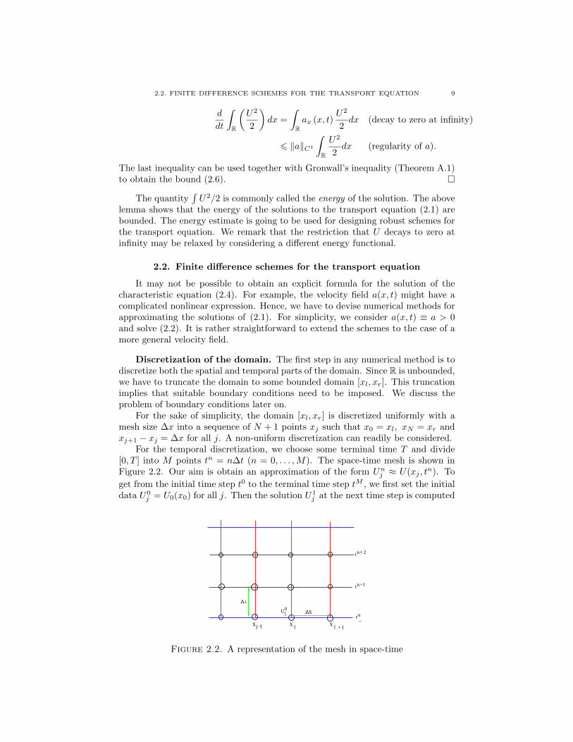
For the temporal discretization, we choose some terminal time T and divide[0, T ] into M points tn = n∆t (n = 0, . . . ,M). The space-time mesh is shown inFigure 2.2. Our aim is obtain an approximation of the form Unj ≈ U(xj , t
n). To
get from the initial time step t0 to the terminal time step tM , we first set the initialdata U0
j = U0(x0) for all j. Then the solution U1j at the next time step is computed
_tn
tn+1
tn+ 2
X j X j + 1Xj−1
Unj ∆
∆ t
X
Figure 2.2. A representation of the mesh in space-time
10 2. LINEAR TRANSPORT EQUATIONS
using some update formula, again for all j. This process is reiterated until we arriveat the final time step tM = T with our final solution UMj .
A simple centered finite difference scheme. On the mesh, we need toapproximate the transport equation (2.2). We do so by replacing both the spatialand temporal derivatives by finite differences. The time derivative is replaced witha forward difference and the spatial derivative with a central difference. This com-bination is standard (see schemes for the heat equation in standard textbooks like[10]). The resulting scheme is
(2.7)Un+1j − Unj
∆t+a(Unj+1 − Unj−1)
2∆x= 0 for j = 1, . . . , N − 1.
Some special care must be taken when defining the boundary values. We have aconsistent discretization of (2.2) that is very simple to implement. We test it onthe following numerical example.
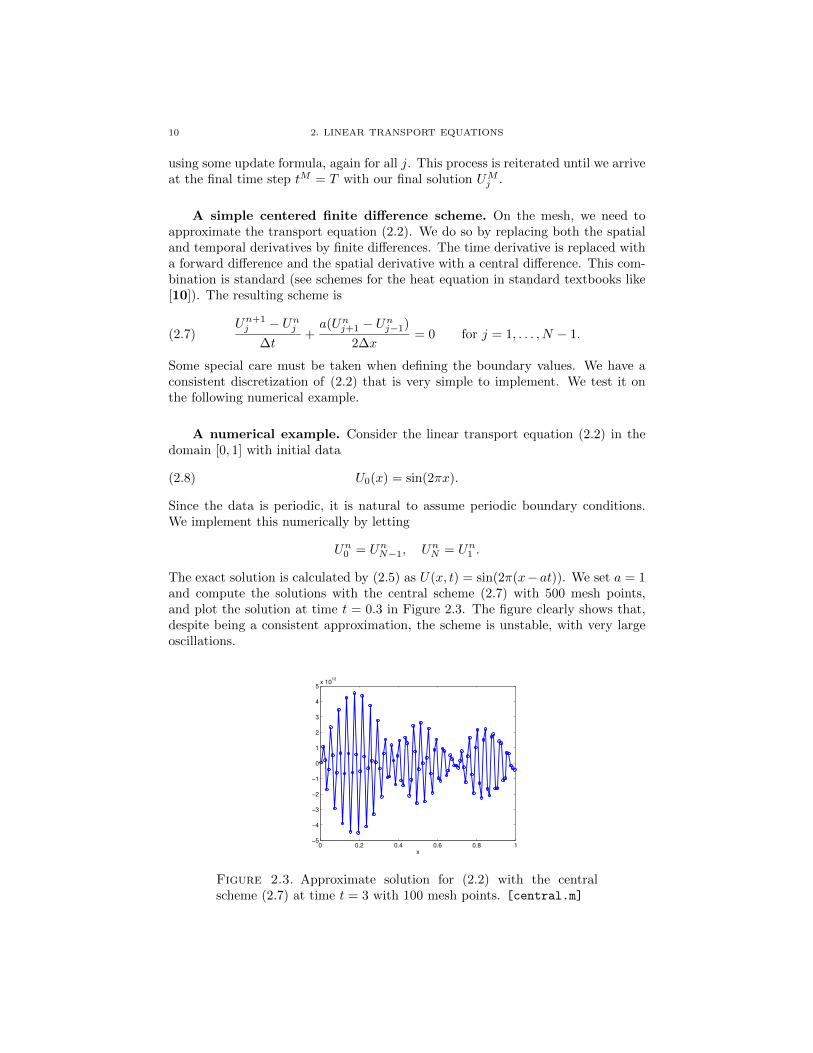
A numerical example. Consider the linear transport equation (2.2) in thedomain [0, 1] with initial data
(2.8) U0(x) = sin(2πx).
Since the data is periodic, it is natural to assume periodic boundary conditions.We implement this numerically by letting
Un0 = UnN−1, UnN = Un1 .
The exact solution is calculated by (2.5) as U(x, t) = sin(2π(x− at)). We set a = 1and compute the solutions with the central scheme (2.7) with 500 mesh points,and plot the solution at time t = 0.3 in Figure 2.3. The figure clearly shows that,despite being a consistent approximation, the scheme is unstable, with very largeoscillations.
0 0.2 0.4 0.6 0.8 1−5
−4
−3
−2
−1
0
1
2
3
4
5x 10
12
x
Figure 2.3. Approximate solution for (2.2) with the centralscheme (2.7) at time t = 3 with 100 mesh points. [central.m]
2.2. FINITE DIFFERENCE SCHEMES FOR THE TRANSPORT EQUATION 11
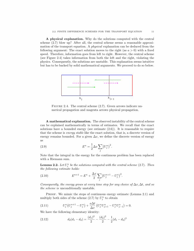
A physical explanation. Why do the solutions computed with the centralscheme (2.7) blow up? After all, the central scheme seems a reasonable approxi-mation of the transport equation. A physical explanation can be deduced from thefollowing argument: The exact solution moves to the right (as a > 0) with a fixedspeed. Therefore, information goes from left to right. However, the central scheme(see Figure 2.4) takes information from both the left and the right, violating thephysics. Consequently, the solutions are unstable. This explanation seems intuitivebut has to be backed by solid mathematical arguments. We proceed to do so below.
X jX j+ 1
Figure 2.4. The central scheme (2.7). Green arrows indicate nu-merical propagation and magenta arrows physical propagation.
A mathematical explanation. The observed instability of the central schemecan be explained mathematically in terms of estimates. We recall that the exactsolutions have a bounded energy (see estimate (2.6)). It is reasonable to requirethat the scheme is energy stable like the exact solution, that is, a discrete version ofenergy remains bounded. For a given ∆x, we define the discrete version of energyas
(2.9) En =1
2∆x∑j
(Unj)2.
Note that the integral in the energy for the continuous problem has been replacedwith a Riemann sum.
Lemma 2.2. Let Unj be the solutions computed with the central scheme (2.7). Thenthe following estimate holds:
(2.10) En+1 = En +∆x
2
∑j
(Un+1j − Unj
)2.
Consequently, the energy grows at every time step for any choice of ∆x,∆t, and sothe scheme is unconditionally unstable.
Proof. We mimic the steps of continuous energy estimate (Lemma 2.1) andmultiply both sides of the scheme (2.7) by Unj to obtain
(2.11) Unj(Un+1j − Unj
)+a∆t
∆x
(Unj U
nj+1 − Unj Unj−1
)= 0.
We have the following elementary identity:
(2.12) d2(d1 − d2) =(d1)2
2− (d2)2
2− 1
2(d1 − d2)2
12 2. LINEAR TRANSPORT EQUATIONS
for any two numbers d1, d2. We denote
Hj+1/2 = aUnj U
n+1j
2
to reduce (2.11) to
(2.13)
(Un+1j
)22
=(Unj )2
2+
1
2
(Un+1j − Unj
)2 − ∆t
∆x(Hj+1/2 −Hj−1/2).
Summing (2.13) over all j and using zero (or periodic) boundary conditions, theflux term H vanishes by cancellation and we obtain the estimate (2.10).
Although we assumed zero or periodic boundary conditions in the proof of thislemma, a variant of the lemma holds for more general boundary conditions, as forthe continuous setting in Lemma 2.1.
The above lemma provides a mathematical justification for our physical intu-ition. The central scheme leads to a growth of energy at every time step and isunstable. We need to find schemes that posses a discrete version of the energyestimate. This use of rigorous mathematical tools like energy analysis to justifyphysical reasoning will be an essential ingredient of these notes.
2.3. An upwind scheme
The central scheme (2.7) does not respect the direction of propagation of in-formation for the transport equation (2.2). Hence, we must include the correctdirection of information propagation and hope that it stabilizes the scheme. Thisentails using one-sided differences instead of a central difference to approximate thelinear transport equation (2.2).
If a > 0 and the direction of information propagation is from left to right, thenwe can use a backward difference in space to obtain the scheme
(2.14)Un+1j − Unj
∆t+a(Unj − Unj−1)
∆x= 0 for j = 1, . . . , N − 1,
and if a < 0, we can use the forward difference to obtain:
(2.15)Un+1j − Unj
∆t+a(Unj+1 − Unj )
∆x= 0 for j = 1, . . . , N − 1.
Using the notation
a+ = maxa, 0, a− = mina, 0, |a| = a+ − a−,
(2.14) and (2.15) can be written together as
(2.16)Un+1j − Unj
∆t+a+(Unj − Unj−1)
∆x+a−(Unj+1 − Unj )
∆x= 0.
The above scheme takes into account the direction of propagation of information –information is “carried with the wind”. Hence, this scheme is termed as the upwindscheme.
Using the definition of the absolute value and some simple algebraic manipu-lations, the upwind scheme (2.16) can be recast as
(2.17)Un+1j − Unj
∆t+a(Unj+1 − Unj−1)
2∆x=|a|
2∆x(Unj+1 − 2Unj + Unj−1)
2.3. AN UPWIND SCHEME 13
X jX j+ 1
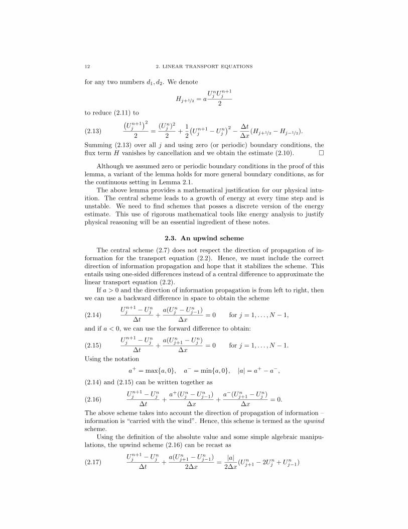
Figure 2.5. The upwind scheme (2.16). Green arrows indicatenumerical propagation and magenta arrows physical propagation.
(compare to (2.7)). Note that in the above form, the spatial derivatives are thecentral term and a diffusion term. The right hand side of (2.17) approximates∆x|a|
2 Uxx. Hence, the upwind scheme (2.17) adds numerical viscosity or diffusionto the unstable central scheme (2.7). Numerical viscosity is going to play a crucialrole later on.
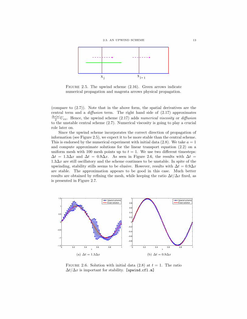
Since the upwind scheme incorporates the correct direction of propagation ofinformation (see Figure 2.5), we expect it to be more stable than the central scheme.This is endorsed by the numerical experiment with initial data (2.8). We take a = 1and compute approximate solutions for the linear transport equation (2.2) on auniform mesh with 100 mesh points up to t = 1. We use two different timesteps:∆t = 1.3∆x and ∆t = 0.9∆x. As seen in Figure 2.6, the results with ∆t =1.3∆x are still oscillatory and the scheme continues to be unstable. In spite of theupwinding, stability stills seems to be elusive. However, results with ∆t = 0.9∆xare stable. The approximation appears to be good in this case. Much betterresults are obtained by refining the mesh, while keeping the ratio ∆t/∆x fixed, asis presented in Figure 2.7.
0 0.2 0.4 0.6 0.8 1−1.5
−1
−0.5
0
0.5
1
1.5
x
Upwind scheme
Exact solution
(a) ∆t = 1.3∆x
0 0.2 0.4 0.6 0.8 1−1
−0.8
−0.6
−0.4
−0.2
0
0.2
0.4
0.6
0.8
1
x
Upwind scheme
Exact solution
(b) ∆t = 0.9∆x
Figure 2.6. Solution with initial data (2.8) at t = 1. The ratio∆t/∆x is important for stability. [upwind cfl.m]
14 2. LINEAR TRANSPORT EQUATIONS
0 0.2 0.4 0.6 0.8 1−1
−0.8
−0.6
−0.4
−0.2
0
0.2
0.4
0.6
0.8
1
x
Upwind scheme
Exact solution
(a) 50 mesh points
0 0.2 0.4 0.6 0.8 1−1
−0.8
−0.6
−0.4
−0.2
0
0.2
0.4
0.6
0.8
1
x
Upwind scheme
Exact solution
(b) 200 mesh points
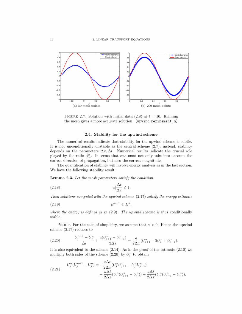
Figure 2.7. Solution with initial data (2.8) at t = 10. Refiningthe mesh gives a more accurate solution. [upwind refinement.m]
2.4. Stability for the upwind scheme
The numerical results indicate that stability for the upwind scheme is subtle.It is not unconditionally unstable as the central scheme (2.7); instead, stabilitydepends on the parameters ∆x,∆t. Numerical results indicate the crucial roleplayed by the ratio ∆t
∆x . It seems that one must not only take into account thecorrect direction of propagation, but also the correct magnitude.
The quantification of stability will involve energy analysis as in the last section.We have the following stability result:
Lemma 2.3. Let the mesh parameters satisfy the condition
(2.18) |a|∆t∆x6 1.
Then solutions computed with the upwind scheme (2.17) satisfy the energy estimate
(2.19) En+1 6 En,
where the energy is defined as in (2.9). The upwind scheme is thus conditionallystable.
Proof. For the sake of simplicity, we assume that a > 0. Hence the upwindscheme (2.17) reduces to
(2.20)Un+1j − Unj
∆t+a(Unj+1 − Unj−1)
2∆x=
a
2∆x(Unj+1 − 2Unj + Unj−1).
It is also equivalent to the scheme (2.14). As in the proof of the estimate (2.10) wemultiply both sides of the scheme (2.20) by Unj to obtain
(2.21)Unj (Un+1
j − Unj ) = − a∆t
2∆x(Unj U
nj+1 − Unj Unj−1)
+a∆t
2∆x(Unj (Unj+1 − Unj )) +
a∆t
2∆x(Unj (Unj−1 − Unj )).
2.4. STABILITY FOR THE UPWIND SCHEME 15
Now we use elementary identity (2.12) a couple of times and rewrite (2.21) as
(2.22)
(Un+1j )2
2=
(Unj )2
2+
(Un+1j − Unj )2
2− a∆t
2∆x(Unj U
nj+1 − Unj Unj−1)
+a∆t
4∆x
((Unj+1)2 − (Unj )2
)− a∆t
4∆x
((Unj )2 − (Unj−1)2
)− a∆t
4∆x(Unj+1 − Unj )2 − a∆t
4∆x(Unj − Unj−1)2.
Denoting
Kj+1/2 =a
2(Unj U
nj+1)− a
4
((Unj+1)2 − (Unj )2
),
we may rewrite (2.22) as
(2.23)
(Un+1j )2
2=
(Unj )2
2+
(Un+1j − Unj )2
2− a∆t
∆x(Kj+1/2 −Kj−1/2)
− a∆t
4∆x(Unj+1 − Unj )2 − a∆t
4∆x(Unj − Unj−1)2.
Summing (2.23) over all j and using the definition of discrete energy (2.9) andeither zero or periodic boundary conditions, we obtain
(2.24) En+1 6 En +∆x
2
∑j
(Un+1j − Unj )2 − a∆t
2
∑j
(Unj − Unj−1)2.
Using the definition of the upwind scheme (2.14) in (2.24) yields
(2.25) En+1 6 En +
(a2∆t2
2∆x− a∆t
2
)∑j
(Unj − Unj−1)2.
Since the term in the sum in (2.25) is positive, we obtain the energy bound (2.19),provided
a2∆t2
∆x6 a∆t,
which is precisely the condition (2.18).
The stability condition (2.18) is termed the CFL condition after Courant,Friedrichs and Lewy who first proposed it. The conditional stability of the up-wind scheme is confirmed in numerical experiments.
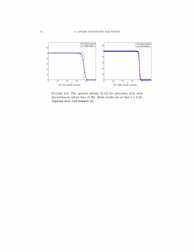
Numerical experiment: Discontinuous data. Consider the transport equa-tion (2.2) with a = 1 in the domain [0, 1] and initial data
(2.26) U0(x) =
2 if x < 0.5
1 if x > 0.5.
The initial data and consequently the exact solution (2.5) are discontinuous. Wecompute with the upwind scheme using 50 and 200 mesh points and display theresults in Figure 2.8. The results show that the upwind scheme approximates thesolution quite well, at least at a fine resolution. However the errors on a coarsemesh are somewhat large. This issue will be addressed in later sections.
16 2. LINEAR TRANSPORT EQUATIONS
0 0.2 0.4 0.6 0.8 11
1.2
1.4
1.6
1.8
2
2.2
x
Upwind scheme
Exact solution
(a) 50 mesh points
0 0.2 0.4 0.6 0.8 11
1.2
1.4
1.6
1.8
2
2.2
x
Upwind scheme
Exact solution
(b) 200 mesh points
Figure 2.8. The upwind scheme (2.14) for advection (2.2) withdiscontinuous initial data (2.26). Both results are at time t = 0.25.[upwind disc refinement.m]
CHAPTER 3
Scalar conservation laws
In the previous section, we considered the scalar transport equation
(3.1) Ut + a(x, t)Ux = 0.
This equation is linear as the velocity field a is a given function. However, mostnatural phenomena are nonlinear. In such models, the linear velocity field must bereplaced with a field that depends on the solution itself. The simplest example ofsuch a field is
a(x, t) = U(x, t).
Hence, the transport equation (3.1) becomes
(3.2) Ut + UUx = 0.
The transport equation (3.2) can be written in the conservative form
(3.3) Ut +
(U2
2
)x
= 0.
This is the inviscid Burgers equation. It serves as a prototype for scalar conserva-tion laws, which in general take the form
(3.4) Ut + f(U)x = 0,
where U is the unknown and f is the flux function. Apart from Burgers’ equation,scalar conservation laws arise in a wide variety of models. We consider a couple ofexamples below.
Traffic flow model. For simplicity, consider a one-dimensional highway anddenote the density of cars (number of cars per square meter) as U(x, t). Assumethat the cars are moving at a macroscopic velocity (the speed of a traffic column)V (x, t). A simple requirement of conservation of the number of cars lead to thefollowing equation:
(3.5) Ut + (UV )x = 0.
The velocity V remains to be modeled. One very simple model is based on a coupleof observations. First, there exists a maximum velocity at which an individual carcan drive, for example specified by the speed limit. Second, the velocity of cars isinversely proportional to the car density. If there are a large number of cars, eachindividual driver will drive slowly. However, on a remote stretch of the highway,each driver speeds up. These simple observations are combined to yield the velocity
V = Vmax(1− U),
where Vmax is the maximum velocity for the cars. We use the convention that themaximum density or road carrying capacity is 1. Hence, the traffic flow equation is
(3.6) Ut +(VmaxU(1− U)
)x
= 0.
17
18 3. SCALAR CONSERVATION LAWS
Enhanced oil recovery. Oil is generally found in sub-surface reservoirs, in-side permeable rocks. The primary stage of oil recovery consists of drilling intothe rocks and extracting oil by applying pressure. Only 20 to 30 percent of theavailable oil can be extracted in this manner. The secondary stage of oil recoveryconsists of injecting water into the rock bed. The water displaces the oil (as wateris heavier) and the oil can then be extracted. This complex process is modeled byusing two-phase flow (water and oil) in a porous media (rock).
For simplicity, we assume that the reservoir is one-dimensional. The quanti-ties of interest are the oil and water volume fractions or saturations So and Sw,respectively. Being volume fractions, they satisfy
(3.7) So + Sw ≡ 1.
Furthermore, the phases evolve according to the conservation laws
(3.8)
Sot + V ox = 0
Swt + V wx = 0.
The phase velocities V o, V w are modeled by Darcy’s law:
(3.9)
V o = −λo dP
o
dx
V w = −λw dPw
dx ,
where λ and P are the phase mobility and the phase pressure, respectively. In theabove constitutive relation, we have neglected the role of gravity. Furthermore, wecan assume that there is no capillary pressure:
P o = Pw.
Adding the phase saturation equations (3.8) for each phase and using the require-ment (3.7), we obtain
(V o + V w)x ≡ 0 ⇒ V o + V w = q,
for some constant q called the total flow rate. Substituting Darcy’s law (3.9) in theabove identity and using Pw = P o = P , we obtain
dP
dx= − q
λo + λw.
Applying this identity in the evolution of the oil saturation (3.9) and (3.8) yields
(3.10) Sot +
(qλo
λw + λo
)x
= 0.
The mobilities generally take the form
λo = (So)2, λw = (Sw)2 = (1− So)2.
Hence, the evolution of the oil saturation is governed by the scalar conservation law
(3.11) Sot +
(q(So)2
(So)2 + (1− So)2
)x
= 0.
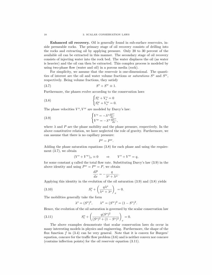
The above examples demonstrate that scalar conservation laws do occur inmany interesting models in physics and engineering. Furthermore, the shape of theflux function f in (3.4) can be very general. Note that it is convex for Burgers’equation, concave for the traffic flow problem (3.6) and is neither convex nor concave(contains inflection points) for the oil reservoir equation (3.11).
3.1. CHARACTERISTICS FOR BURGER’S EQUATION 19
In this section, we embark on a systematic study of scalar conservation laws(3.4) from a theoretical perspective.
3.1. Characteristics for Burger’s equation
We start with Burgers’ equation (3.3) and attempt to construct solutions to theinitial value problem associated with it. As for the linear transport equation (3.1),we will use the method of characteristics for this purpose. Since (3.2) and (3.3) areequivalent whenever U is smooth, the characteristics x(t) for Burgers’ equation aregiven by
x′(t) = U(x(t), t)
x(0) = x0.(3.12)
Note that these characteristics are different from the linear case (2.4) in that thevelocity depends on the solution. We consider initial data
(3.13) U0(x) =
Ul if x < 0
Ur if x > 0.
Data of this form is quite simple and consists of constants separated by a discon-tinuity at the origin. The initial value problem for a conservation law (3.4) withinitial data of the form (3.13) is called a Riemann problem.
By definition, the solution U is constant along characteristics, that is, U(x(t), t) =U0(x0). Therefore, the solution of (3.12), (3.13) in constant parts of U0 is
x(t) = U0(x0)t+ x0.
Let Ul = 1 and Ur = 0 in (3.13). For x0 < 0 the characteristics have velocityU0(x0) = 1, whereas for x0 > 0 they have velocity 0; see Figure 3.1. We see thatthe characteristics intersect almost instantaneously. As observed in the last section,the solution should be constant (in time) along the characteristics. What happensto the solution when the characteristics start to intersect? How can the solutionbe defined in this case? Adding nonlinearity completely changes the situation fromthe linear case.
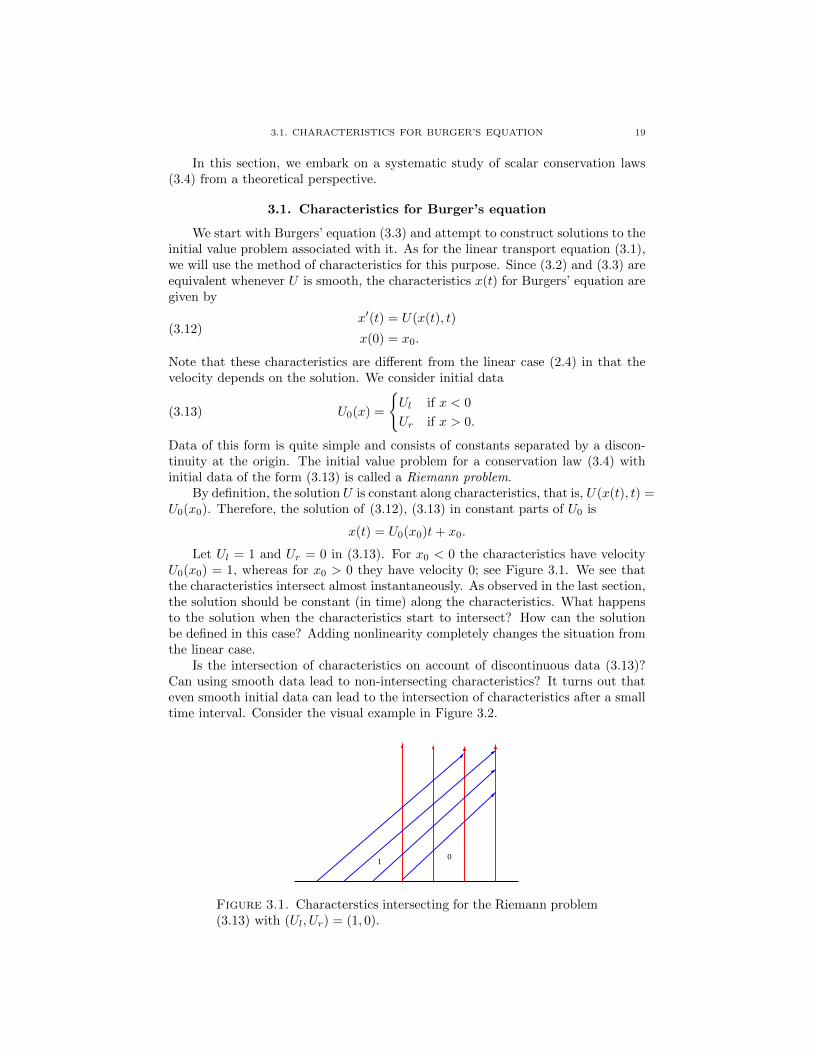
Is the intersection of characteristics on account of discontinuous data (3.13)?Can using smooth data lead to non-intersecting characteristics? It turns out thateven smooth initial data can lead to the intersection of characteristics after a smalltime interval. Consider the visual example in Figure 3.2.
01
Figure 3.1. Characterstics intersecting for the Riemann problem(3.13) with (Ul, Ur) = (1, 0).
20 3. SCALAR CONSERVATION LAWS
X
U0(X)
(a) Initial data (b) Characteristics
Figure 3.2. Characteristics can even intersect for smooth initial data.
Exercise 3.1. Let U0(x) be differentiable with at least one point x such that U ′0(x) <0. Show that the solution to Burgers’ equation with initial data U0 will develop adiscontinuity at time
tmin = − 1
minx∈R U ′0(x).
(Hint: Start with the ansatz that two characteristics x(t) and x(t) intersect at sometime t.)
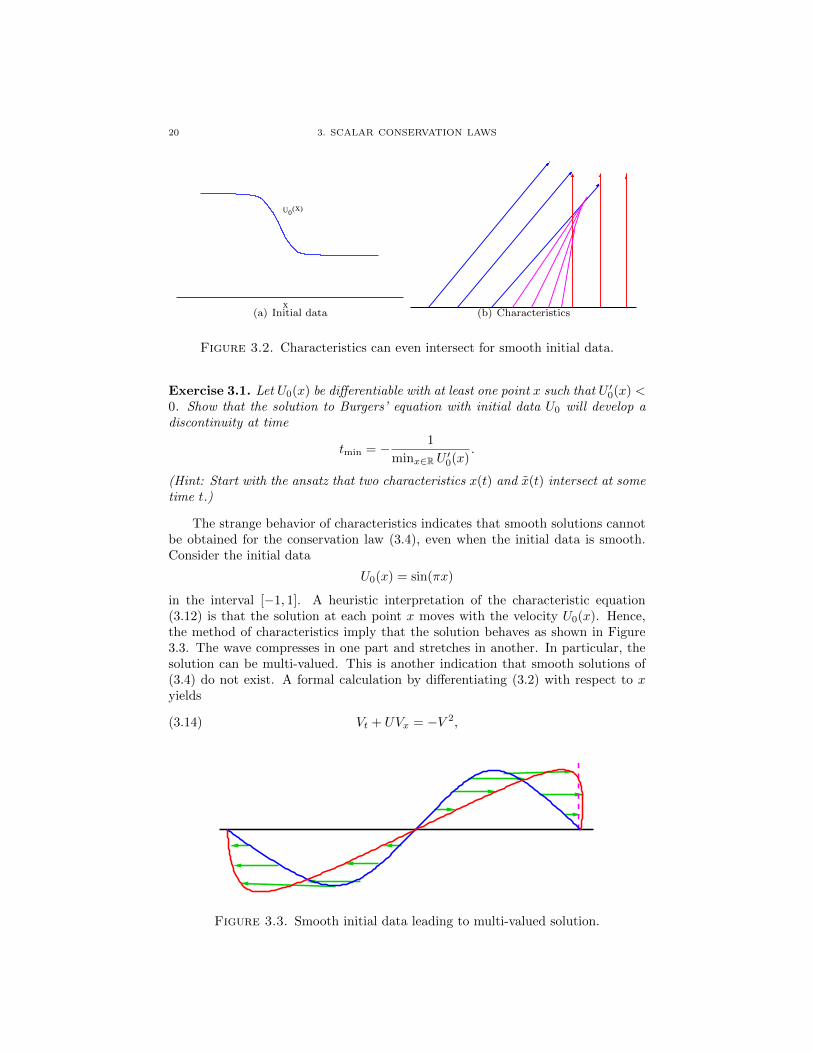
The strange behavior of characteristics indicates that smooth solutions cannotbe obtained for the conservation law (3.4), even when the initial data is smooth.Consider the initial data
U0(x) = sin(πx)
in the interval [−1, 1]. A heuristic interpretation of the characteristic equation(3.12) is that the solution at each point x moves with the velocity U0(x). Hence,the method of characteristics imply that the solution behaves as shown in Figure3.3. The wave compresses in one part and stretches in another. In particular, thesolution can be multi-valued. This is another indication that smooth solutions of(3.4) do not exist. A formal calculation by differentiating (3.2) with respect to xyields
(3.14) Vt + UVx = −V 2,
Figure 3.3. Smooth initial data leading to multi-valued solution.
3.2. WEAK SOLUTIONS 21
where V = Ux. Hence, along the characteristics x(t) given by (3.12), V varies as
d
dtV (x(t), t) = −V 2(x(t), t).
This is a ODE with quadratic nonlinearity and it is well known that the resultingsolution V can blow up in finite time. Hence, the spatial derivative of the solutionto Burgers’ equation can blow up, even if the initial derivative is very small. Thisderivative blowup suggests that smooth solutions to (3.4) may not exist.
3.2. Weak solutions
The previous section demonstrates that smooth or classical solutions of theconservation law (3.4) may not exist. However, these models arise in physics andso some form of solution does exist. This type of solution is a weak solution. Tomotivate the definition of weak solutions, assume for the moment that smoothsolutions of (3.4) exist and multiply both sides by a smooth test function ϕ ∈C1c (R×R+). The space C1
c is the space of all continuously differentiable functionswith compact support, that is, the functions vanish outside a compact subset ofthe domain. Using integration by parts, (3.4) reduces to
(3.15)
∫R×R+
Uϕt + f(U)ϕx dxdt+
∫RU0(x)ϕ(x, 0) dx = 0.
This identity hold trues for all test functions ϕ. We base the definition of weaksolution for (3.4) on the above identity.
Definition 3.2 (Weak solution). A function U ∈ L1(R × R+) is a weak solutionof (3.4) if the identity (3.15) holds for all test functions ϕ ∈ C1
c (R× R+).
Note that the identity (3.15) is well-defined as long as U ∈ L∞(R× R+).
Exercise 3.3. Show that if a weak solution U of (3.4) is also differentiable (soU ∈ C1(R × R+)), then U satisfies (3.4) point-wise. Hence, the class of weaksolutions contains, but is not restricted to, classical solutions.
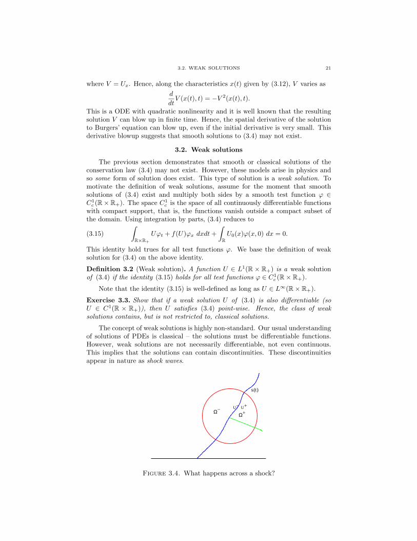
The concept of weak solutions is highly non-standard. Our usual understandingof solutions of PDEs is classical – the solutions must be differentiable functions.However, weak solutions are not necessarily differentiable, not even continuous.This implies that the solutions can contain discontinuities. These discontinuitiesappear in nature as shock waves.
Ω− Ω+
− U U+
s(t)
Figure 3.4. What happens across a shock?
22 3. SCALAR CONSERVATION LAWS
3.2.1. The Rankine-Hugoniot condition. As we will soon find out, shockwaves in weak solutions cannot be arbitrary curves in the x-t-plane, but must satisfycertain conditions. Assume that we are given a weak solution U consisting of twosmooth regions, separated by a shock wave, as depicted in Figure 3.4. Let the shockwave be defined by the curve x = σ(t).
Let ϕ be a test function with support in Ω. We assume that U ∈ C1(Ω−) andU ∈ C1(Ω+); see Figure 3.4. Integrating (3.15) by parts and using the compactsupport of the test function, we get∫
Ω
Uϕt + f(U)ϕx dΩ =
∫Ω+
Uϕt + f(U)ϕx dΩ +
∫Ω−
Uϕt + f(U)ϕx dΩ
= −∫
Ω+
(Ut + f(U)x)ϕ dΩ +
∫∂Ω+
(U+(t)νt + f(U+(t))νx)ϕ dΩ
−∫
Ω−(Ut + f(U)x)ϕ dΩ +
∫∂Ω−
(U−(t)νt + f(U−(t))νx)ϕ dΩ
= 0.
Here, U+(t) and U−(t) are the trace values of U on the right and left of thediscontinuity σ, and ν is the unit outward normal of σ (see Figure 3.4). We have
(νt, νx) = (−s(t), 1),
where s(t) = σ′(t) is the speed of the shock curve. Since U is smooth in Ω− andΩ+, the equation (3.4) is satisfied point-wise. Therefore, the above identities implythat∫
Ω−∪Ω+
(Ut + f(U)x
)︸ ︷︷ ︸= 0
ϕ dΩ +
∫∂Ω
(s(t)
(U+(t)− U−(t)
)−(f(U+)− f(U−)
))ϕ dΩ = 0.
Since ϕ is an arbitrary test function, the integrand of the remaining integral mustbe identically equal to zero. Hence, the shock speed must satisfy
(3.16) s(t) =f(U+(t))− f(U−(t))
U+(t)− U−(t).
This condition is called the Rankine-Hugoniot condition.
3.2.2. Solutions to Riemann problems. Consider Burgers’ equation (3.3)with the Riemann problem (3.13) with Ul = 1 and Ur = 0. We recall that the char-acteristics intersected in this case and a smooth solution couldn’t be constructed.We construct a weak solution that consists of two constant states Ul and Ur, sep-arated by a shock moving at a speed given by the Rankine-Hugoniot condition(3.16),
s(t) =U2r − U2
l
2(Ur − Ul)≡ 1
2.
Hence, the weak solution takes the form
(3.17) U(x, t) =
1 if x < 1
2 t
0 if x > 12 t.
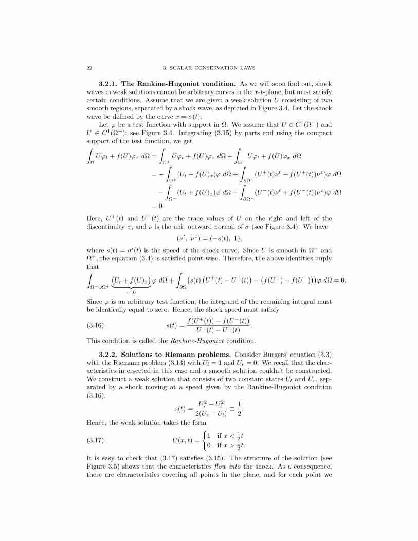
It is easy to check that (3.17) satisfies (3.15). The structure of the solution (seeFigure 3.5) shows that the characteristics flow into the shock. As a consequence,there are characteristics covering all points in the plane, and for each point we
3.2. WEAK SOLUTIONS 23
can trace a characteristic back to the initial data. Hence, the entire solution isprescribed by the initial data.
x
t
Figure 3.5. Characteristics for the Riemann problem (3.17).
x
t
?
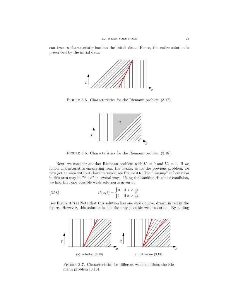
Figure 3.6. Characteristics for the Riemann problem (3.18).
Next, we consider another Riemann problem with Ul = 0 and Ur = 1. If wefollow characteristics emanating from the x-axis, as for the previous problem, wenow get an area without characteristics; see Figure 3.6. The ”missing” informationin this area may be ”filled” in several ways. Using the Rankine-Hugoniot condition,we find that one possible weak solution is given by
(3.18) U(x, t) =
0 if x < 1
2 t
1 if x > 12 t,
see Figure 3.7(a) Note that this solution has one shock curve, drawn in red in thefigure. However, this solution is not the only possible weak solution. By adding
x
t
(a) Solution (3.18)
x
t
(b) Solution (3.19)
Figure 3.7. Characteristics for different weak solutions the Rie-mann problem (3.18).
24 3. SCALAR CONSERVATION LAWS
an intermediate state with value, say, Um = 23 and using the Rankine-Hugoniot
condition, we get the weak solution
(3.19) U(x, t) =
0, if x < 1
3 t23 if 1
3 t < x < 56 t
1 if x > 56 t.
The characteristics are shown in Figure 3.7(b). In a similar manner one may con-struct arbitrarily many weak solutions by using the Rankine-Hugoniot condition(3.16) with different intermediate states.
This problem of non-uniqueness is implicit in the definition of weak solutions.These solutions are not necessarily unique, and therefore some extra conditions needto be imposed. For finding these extra criteria, we observe that characteristics forboth (3.18) and (3.19) flow out from the shock (see Figure 3.7). This is in contrastto the solution (3.17) where the characteristics flow into the shock (see Figure 3.5).Characteristics represent the flow of information. For an evolution equation theinformation should always flow from the initial data. This is clearly the case forthe weak solution (3.17). However in the case of weak solutions (3.18) and (3.19),information seems to be created at the shock.
This heuristic requirement, that information is taken from the initial data and isnot created at a shock, can be expressed in terms of conditions on the characteristicsacross a shock. Let U−(t), U+(t) be the states on either side of a shock with speeds(t). The requirement that characteristics for Burgers’ equation flow into the shockand information is taken from the initial line can be enforced by the condition
(3.20) U−(t) > s(t) > U+(t).
It is simple to generalize (3.20) to the general scalar conservation law (3.4) forconvex f :
(3.21) f ′(U−(t)) > s(t) > f ′(U+(t)).
This is the Lax entropy condition.Consider the conservation law (3.4) with a convex flux function and Riemann
data (3.13). It is easily shown that
(3.22) U(x, t) =
Ul if x < st
Ur if x > st,
where the shock speed s is defined by the Rankine-Hugoniot condition, is a weaksolution of (3.4). Now, there are two cases: either Ul > Ur, or Ul < Ur. It turnsout that the Lax entropy condition excludes (3.22) as a solution in the latter case,but not in the former:
Exercise 3.4. Assume that f is strictly convex and that Ul > Ur. Show that (3.22)is a weak solution that satisfies the entropy condition (3.21). Similarly, if Ul < Ur,show that (3.22) is a weak solution, but does not satisfy Lax’ entropy condition.
It turns out that in the latter case, where Ul < Ur, a continuous (but notnecessarily differentiable) solution exists.
3.2. WEAK SOLUTIONS 25
3.2.3. Rarefaction waves. For the remainder of this section, assume thatthe flux function f is strictly convex. In order to construct a continuous solutionto (3.4), we note that replacing x, t by λx, λt keeps the equation invariant, in thesense that a solution of one is a solution of the other. Hence, it is natural to assumeself-similarity – that solutions only depend on the ratio x/t:
(3.23) U(x, t) = V (x/t) .
Define the similarity variable ξ = x/t. We substitute the ansatz (3.23) into (3.4)and use the chain rule repeatedly to obtain
Vt + f(V )x = V (ξ)t + f ′(V (ξ))V (ξ)x
= Vξξt + f ′(V (ξ))Vξξx
= − xt2Vξ + f ′(V (ξ))
1
tVξ = 0
⇒(f ′(V (ξ))− x
t
)Vξ = 0.
In the nontrivial case of Vξ 6= 0, the above identity and the fact that f ′ is strictlyincreasing (recall that f is assumed to be strictly convex) leads to the expression
(3.24) V (x/t) = (f ′)−1(x/t).
A self-similar solution of this form is called a rarefaction wave.The rarefaction wave can be employed to construct weak solutions for conser-
vation laws. Consider the Riemann problem (3.4), (3.13). If Ul < Ur, then theweak solution is given by
(3.25) U(x, t) =
Ul if x 6 f ′(Ul)t
(f ′)−1(x/t) if f ′(Ul)t < x 6 f ′(Ur)t
Ur if x > f ′(Ur)t.
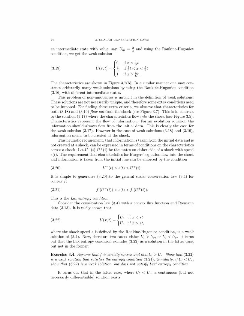
Clearly (3.25) is a weak solution that satisfies Lax’ entropy condition (3.21). Forthe particular case of Burgers’ equation with Riemann data Ul = 0 and Ur = 1, thesolution (3.25) is shown in Figure 3.8. Note how the characteristics are parallel tothe rarefaction wave and contrast this to Figure 3.7.
x
t
Figure 3.8. The rarefaction solution (3.25)
We now have a recipe to construct weak solutions for the Riemann problem(3.13) for a conservation law (3.4) with a strictly convex f . The solution dependson whether Ul < Ur or Ul > Ur. If Ul > Ur, then the entropy satisfying weaksolution (3.22) consists of a shock between the two states. If Ul < Ur, then theweak solution (3.25) consists of the two states, separated by a rarefaction wave.
26 3. SCALAR CONSERVATION LAWS
In both cases, the wave speed is bounded in absolute value by the maximum of|f ′(Ul)| and |f ′(Ur)|.
It remains to solve the Riemann problem when the flux is not strictly convex.
3.2.4. Solutions to the Riemann problem in the general case. We needto generalize the entropy condition (3.20) when the flux is no longer strictly convex.This is done by the following condition.
Definition 3.5 (Oleinik entropy condition). Let U be a weak solution of (3.4), andlet Ul, Ur be the trace values at a shock with speed s. (All of these quantities dependon t, but we drop the time dependence for notational convenience.) The solutionsatisfies the Oleinik entropy condition if
s 6f(k)− f(Ul)
k − Ulfor all k between Ul and Ur.
Exercise 3.6. Use the Rankine-Hugoniot condition to show that U satisfies theOleinik entropy condition if and only if
f(k)− f(Ur)
k − Ur6 s
for all k between Ul and Ur.
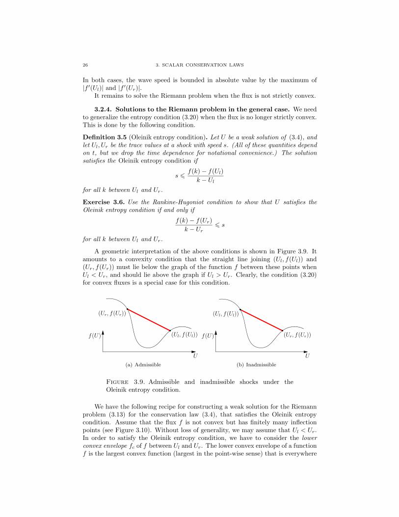
A geometric interpretation of the above conditions is shown in Figure 3.9. Itamounts to a convexity condition that the straight line joining (Ul, f(Ul)) and(Ur, f(Ur)) must lie below the graph of the function f between these points whenUl < Ur, and should lie above the graph if Ul > Ur. Clearly, the condition (3.20)for convex fluxes is a special case for this condition.
U
f(U)
(Ur, f(Ur))
(Ul, f(Ul))
(a) Admissible
U
f(U)
(Ul, f(Ul))
(Ur, f(Ur))
(b) Inadmissible
Figure 3.9. Admissible and inadmissible shocks under theOleinik entropy condition.
We have the following recipe for constructing a weak solution for the Riemannproblem (3.13) for the conservation law (3.4), that satisfies the Oleinik entropycondition. Assume that the flux f is not convex but has finitely many inflectionpoints (see Figure 3.10). Without loss of generality, we may assume that Ul < Ur.In order to satisfy the Oleinik entropy condition, we have to consider the lowerconvex envelope fc of f between Ul and Ur. The lower convex envelope of a functionf is the largest convex function (largest in the point-wise sense) that is everywhere
3.3. ENTROPY SOLUTIONS 27
(Ul, f(Ul)) (Ur, f(Ur))
U
f(U)
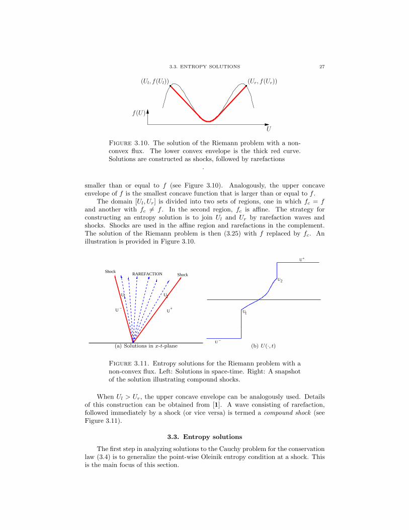
Figure 3.10. The solution of the Riemann problem with a non-convex flux. The lower convex envelope is the thick red curve.Solutions are constructed as shocks, followed by rarefactions
.
smaller than or equal to f (see Figure 3.10). Analogously, the upper concaveenvelope of f is the smallest concave function that is larger than or equal to f .
The domain [Ul, Ur] is divided into two sets of regions, one in which fc = fand another with fc 6= f . In the second region, fc is affine. The strategy forconstructing an entropy solution is to join Ul and Ur by rarefaction waves andshocks. Shocks are used in the affine region and rarefactions in the complement.The solution of the Riemann problem is then (3.25) with f replaced by fc. Anillustration is provided in Figure 3.10.
U −
U1
U2
U+
ShockShockRAREFACTION
(a) Solutions in x-t-planeU −
U1
U2
U+
(b) U(·, t)
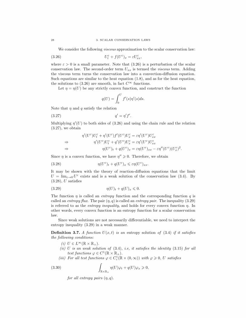
Figure 3.11. Entropy solutions for the Riemann problem with anon-convex flux. Left: Solutions in space-time. Right: A snapshotof the solution illustrating compound shocks.
When Ul > Ur, the upper concave envelope can be analogously used. Detailsof this construction can be obtained from [1]. A wave consisting of rarefaction,followed immediately by a shock (or vice versa) is termed a compound shock (seeFigure 3.11).
3.3. Entropy solutions
The first step in analyzing solutions to the Cauchy problem for the conservationlaw (3.4) is to generalize the point-wise Oleinik entropy condition at a shock. Thisis the main focus of this section.
28 3. SCALAR CONSERVATION LAWS
We consider the following viscous approximation to the scalar conservation law:
(3.26) Uεt + f(Uε)x = εUεxx,
where ε > 0 is a small parameter. Note that (3.26) is a perturbation of the scalarconservation law. The second-order term Uxx is termed the viscous term. Addingthe viscous term turns the conservation law into a convection-diffusion equation.Such equations are similar to the heat equation (1.8), and as for the heat equation,the solutions to (3.26) are smooth, in fact C∞ functions.
Let η = η(U) be any strictly convex function, and construct the function
q(U) =
∫ U
0
f ′(s)η′(s)ds.
Note that η and q satisfy the relation
(3.27) q′ = η′f ′.
Multiplying η′(U) to both sides of (3.26) and using the chain rule and the relation(3.27), we obtain
η′(Uε)Uεt + η′(Uε)f ′(Uε)Uεx = εη′(Uε)Uεxx
⇒ η′(Uε)Uεt + q′(Uε)Uεx = εη′(Uε)Uεxx
⇒ η(Uε)t + q(Uε)x = εη(Uε)xx − εη′′(Uε)(Uεx)2.
Since η is a convex function, we have η′′ > 0. Therefore, we obtain
(3.28) η(Uε)t + q(Uε)x 6 εη(Uε)xx.
It may be shown with the theory of reaction-diffusion equations that the limitU = limε→0 U
ε exists and is a weak solution of the conservation law (3.4). By(3.28), U satisfies
(3.29) η(U)t + q(U)x 6 0.
The function η is called an entropy function and the corresponding function q iscalled an entropy flux. The pair (η, q) is called an entropy pair. The inequality (3.29)is referred to as the entropy inequality, and holds for every convex function η. Inother words, every convex function is an entropy function for a scalar conservationlaw.
Since weak solutions are not necessarily differentiable, we need to interpret theentropy inequality (3.29) in a weak manner.
Definition 3.7. A function U(x, t) is an entropy solution of (3.4) if it satisfiesthe following conditions:
(i) U ∈ L∞(R× R+).(ii) U is an weak solution of (3.4), i.e, it satisfies the identity (3.15) for all
test functions ϕ ∈ C1(R× R+).(iii) For all test functions ϕ ∈ C1
c (R× (0,∞)) with ϕ > 0, U satisfies
(3.30)
∫R×R+
η(U)ϕt + q(U)ϕx > 0,
for all entropy pairs (η, q).
3.3. ENTROPY SOLUTIONS 29
Remark 3.8. Any convex function η serves as an entropy function for a scalarconservation law. Of particular importance are the so-called Kruzkhov entropies:
(3.31) η = η(U, k) = |U − k|
for constants k ∈ R. The corresponding entropy flux is
(3.32) q = q(U, k) = sign(U − k)(f(U)− f(k)).
It is straightforward to check that any smooth convex function g(U) can be ap-proximated by a linear combination of functions like η(U, k) on bounded intervalsU ∈ [a, b]. More precisely, given δ > 0, there exist N ∈ N and αk, ck ∈ R with1 6 k 6 N such that∣∣∣g(U)−
N∑k=1
αk|U − ck|∣∣∣ 6 δ for all U ∈ [a, b].
Thus, (3.29) holds if and only if
(3.33) |U − k|t +(sign(U − k)(f(U)− f(k))
)x6 0
(in the weak sense) for all k ∈ R.
It is straightforward to check that the entropy solution satisfies the Oleinikentropy condition (check [1] for a proof). The concept of entropy solutions is thecorrect notion of solutions to conservation laws. We will demonstrate the existenceand uniqueness of entropy solutions in this section.
The entropy inequality (3.29) can be used to obtain estimates on solutions. Tosee this, integrate (3.29) over space and integrate by parts to obtain
(3.34)d
dt
∫Rη(U) 6 0 ⇒
∫Rη(U(x, t))dx 6
∫Rη(U0(x))dx.
Since the function η may be any convex function, we can choose η(U) = U2
2
and obtain a bound on the entropy solution in L2. This estimate is a nonlinearanalogue of the energy estimate (2.6) for the linear transport equation. Choosingη as
η(U) =|U |p
p
will lead to estimates in Lp spaces for all p > 1. Hence, the entropy inequalityserves to yield stability estimates.
A key estimate is the L∞ estimate that bounds the maximum and minimumof the solutions of (3.26). The L∞ estimate is a consequence of the standardmaximum principle for parabolic equations. A formal proof proceeds as follows:Assume that the maximum of the solution U is attained at a point x0 at timet0 > 0. Clearly Ut(x0, t0) = Ux(x0, t0) = 0. Furthermore, as (x0, t0) is a maximum,we can assume that Uxx(x0, t0) < 0. Substituting all these relations in (3.26) leadsto a contradiction. Hence, the maximum can only be attained at the initial data.A similar estimate holds at minima.
Another crucial stability estimate for (3.26) concerns the control of the deriva-tive. To motivate this estimate, we let η(U) = η(U, 0) = |U |, the Kruzkhov entropycentered at 0. Formally we have
η′(U) = sign(U), η′′(U) = δ(U),
30 3. SCALAR CONSERVATION LAWS
where δ is the Dirac mass or delta function centered at 0. Multiplying (3.26) with−η′(Uεx)x and using the chain rule and integrating by parts, we obtain
−∫Rη′(Uεx)xU
εt dx−
∫Rη′(Uεx)xf
′(Uε)Uεxdx = −ε∫Rη′(Uεx)xU
εxxdx∫
Rη′(Uεx)Uεxtdx−
∫Rη′(Uεx)xf
′(Uε)Uεxdx = −ε∫Rη′(Uεx)xU
εxxdx (integration by parts)
d
dt
∫R|Uεx |dx−
∫Rη′′(Uεx)f ′(Uεx)UεxU
εxxdx︸ ︷︷ ︸
=0
= −ε∫Rη′′(Uεx)(Uεxx)2dx (chain rule),
which in the limit ε→ 0 gives us
d
dt
∫R|Ux|dx 6 0.
These computations are formal but can be made completely rigorous (see [1]).Of great importance in the context of conservation laws is the concept of total
variation. Let g be a function defined on an interval [a, b]. The total variation of gis defined as
(3.35) ‖g‖TV = supP
NP−1∑j=1
|g(xj+1)− g(xj)|,
where the supremum is taken over all partitions P = a = x1 < x2 < · · · < xNP =b of the interval [a, b]. It is straightforward to check that if g is differentiable, then
‖g‖TV =
∫ b
a
|gx|dx.
The total variation is only a semi-norm; indeed, the total variation of any constantfunction is zero. We turn it into a norm by defining
(3.36) ‖g‖BV = ‖g‖L1 + ‖g‖TV .
We define the space of functions with bounded variation (BV) as
(3.37) BV (R) =g ∈ L1(R) : ‖g‖BV <∞
.
The above estimate on∫|Ux|dx is a BV estimate. It states that the solutions
to a conservation law (3.4) are Total Variation Diminishing (TVD), that is,
‖U(·, t)‖BV 6 ‖U0‖BV for all t > 0.
We are now in a position to state the main well-posedness results for scalarconservation laws:
Theorem 3.9. If U0 ∈ L∞(R)∩BV (R), then (3.4) has a entropy solution U whichsatisfies the estimates
(3.38) ‖U(·, t)‖L∞ 6 ‖U0‖L∞
and
(3.39) ‖U(·, t)‖TV 6 ‖U0‖TV .
3.3. ENTROPY SOLUTIONS 31
Furthermore, if U and V are entropy solutions of (3.4) with initial U0 and V0,respectively, then
(3.40)
∫R|U(x, t)− V (x, t)|dx 6
∫R|U0(x)− V0(x)|dx for all t > 0.
Hence, entropy solutions are unique.
The proof of this theorem is outside the scope of these notes (consult standardtext books like [1]). We only sketch the main ideas of the proof. The existence isbased on the viscous approximation (3.26). The entropy conditions yield estimateson the solution in Lp spaces as discussed before. Formal arguments for establishingthe L∞ and BV bounds are discussed above. Uniqueness of entropy solutionsrelying on the L1 contraction estimate (3.40) is based on the ingenious doubling ofvariables idea of Kruzkhov [6] and uses the Kruzkhov entropies (3.31) extensively.
Summarizing the theoretical discussion of this section, we have the followingresults:
• Solutions of the conservation law (3.4) may develop discontinuities orshock waves, even for smooth initial data. Consequently, weak solutionsare sought. Shock speeds are computed with the Rankine-Hugoniot con-dition (3.16).
• Weak solutions are not necessarily unique. Entropy conditions like theOleinik entropy conditions have to be imposed. Self-similar continuoussolutions or rarefaction waves have to be considered.
• Explicit solutions for the Riemann problem (even for non-convex fluxes)can be constructed in terms of shocks, rarefaction waves and compoundshocks.
• Entropy solutions exist and are unique. Furthermore, the entropy solu-tions satisfy an L∞ estimate, Lp estimates and are TVD – that is, theBV-norm decreases in time.
Despite the considerable theoretical results, we cannot obtain explicit solutionformulas for more complicated initial data. Hence, we have to design efficientnumerical methods for computing these solutions.

CHAPTER 4
Finite volume schemes for scalar conservation laws
In this chapter we will design efficient schemes for the scalar conservation law
(4.1) Ut + f(U)x = 0.
The discussion on the linear transport equation
(4.2) Ut + aUx = 0
shows that central differences cannot be used to approximate the conservation law,even in the simplest case of linear transport. For linear transport equations, thecrucial step in designing an efficient scheme was to upwind it by taking derivativesin the direction of information propagation. For a linear equation with constantcoefficients like (4.2), the direction of information propagation is given by the con-stant velocity field. For a nonlinear conservation law like (4.1), the wave speedsdepend on the solution itself and can not be determined a priori. Thus, it is notclear how differences can be upwinded.
Another issue is the very nature of finite difference approximations like (2.16).The key idea underlying finite difference schemes is to replace the derivatives inequations like (4.1) with a finite difference. This procedure requires the solutions tobe smooth and the equation to be satisfied point-wise. However, the solutions to thescalar conservation law (4.1) are not necessarily smooth and so the Taylor expansion– essential for replacing derivatives with finite differences – is no longer valid. Hence,the finite difference framework is not suited for approximating conservation laws.Instead, we need to develop a new paradigm for designing numerical schemes forscalar conservation laws.
4.1. Finite volume scheme
The first step in any numerical approximation is to discretize the computationaldomain in both space and time.
4.1.1. The grid. For simplicity, we consider a uniform discretization of thedomain [xL, xR]. The discrete points are denoted as xj = xL + (j + 1/2)∆x forj = 0, . . . , N , where ∆x = xR−xL
N+1 . We also define the midpoint values
xj−1/2 = xj −∆x/2 = xL + j∆x
for j = 0, . . . , N + 1. These values define computational cells or control volumes
Cj =[xj−1/2, xj+1/2
).
As we will see soon, the finite volume method uses the control volumes Cj insteadof the mesh points xj . We use a uniform discretization in time with time step ∆t.The time levels are denoted by tn = n∆t. See Figure 4.1 for an illustration of thegrid.
33
34 4. FINITE VOLUME SCHEMES FOR SCALAR CONSERVATION LAWS
X j 1 Xj +1
t n
tn+1
Unj U
nj+1U
nj −1
Un+1j
Fj +1/2Fj −1/2
− 2/ /2
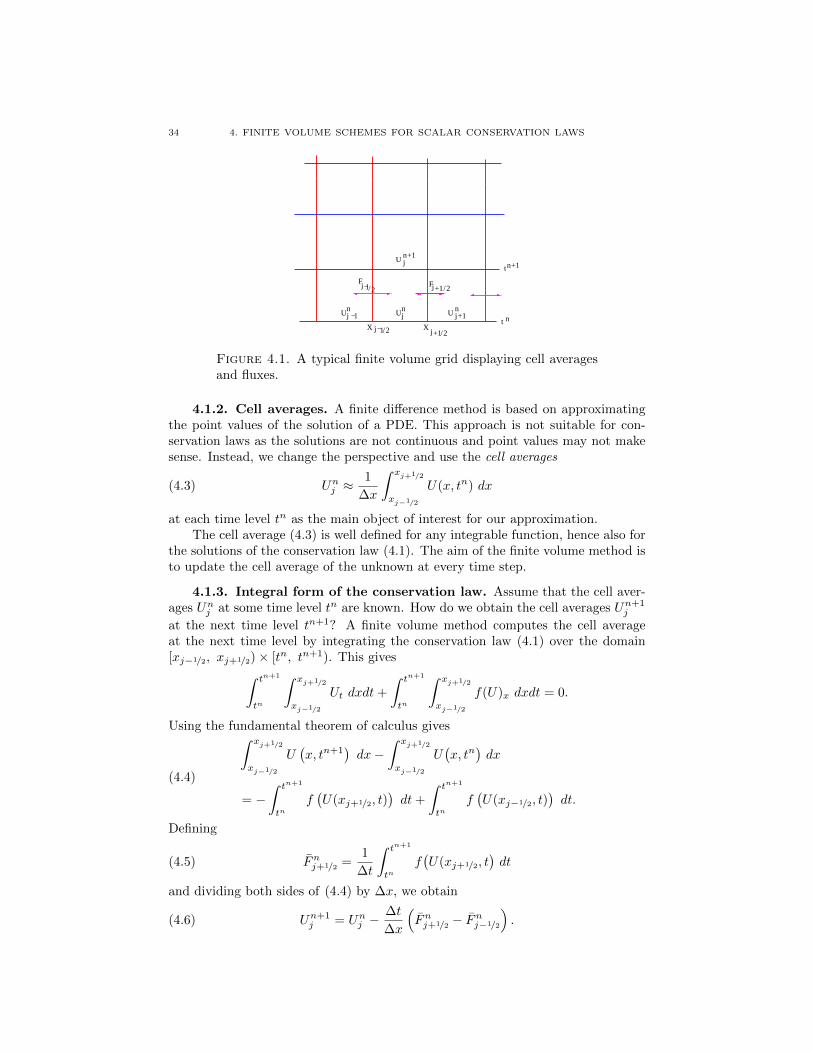
Figure 4.1. A typical finite volume grid displaying cell averagesand fluxes.
4.1.2. Cell averages. A finite difference method is based on approximatingthe point values of the solution of a PDE. This approach is not suitable for con-servation laws as the solutions are not continuous and point values may not makesense. Instead, we change the perspective and use the cell averages
(4.3) Unj ≈1
∆x
∫ xj+1/2
xj−1/2
U(x, tn) dx
at each time level tn as the main object of interest for our approximation.The cell average (4.3) is well defined for any integrable function, hence also for
the solutions of the conservation law (4.1). The aim of the finite volume method isto update the cell average of the unknown at every time step.
4.1.3. Integral form of the conservation law. Assume that the cell aver-ages Unj at some time level tn are known. How do we obtain the cell averages Un+1
j
at the next time level tn+1? A finite volume method computes the cell averageat the next time level by integrating the conservation law (4.1) over the domain[xj−1/2, xj+1/2)× [tn, tn+1). This gives∫ tn+1
tn
∫ xj+1/2
xj−1/2
Ut dxdt+
∫ tn+1
tn
∫ xj+1/2
xj−1/2
f(U)x dxdt = 0.
Using the fundamental theorem of calculus gives∫ xj+1/2
xj−1/2
U(x, tn+1
)dx−
∫ xj+1/2
xj−1/2
U(x, tn
)dx
= −∫ tn+1
tnf(U(xj+1/2, t)
)dt+
∫ tn+1
tnf(U(xj−1/2, t)
)dt.
(4.4)
Defining
(4.5) Fnj+1/2 =1
∆t
∫ tn+1
tnf(U(xj+1/2, t
)dt
and dividing both sides of (4.4) by ∆x, we obtain
(4.6) Un+1j = Unj −
∆t
∆x
(Fnj+1/2 − F
nj−1/2
).
4.1. FINITE VOLUME SCHEME 35
X j −1/2X j + 1 / 2
tn
tn+1
Unj
Unj + 1
Unj −1
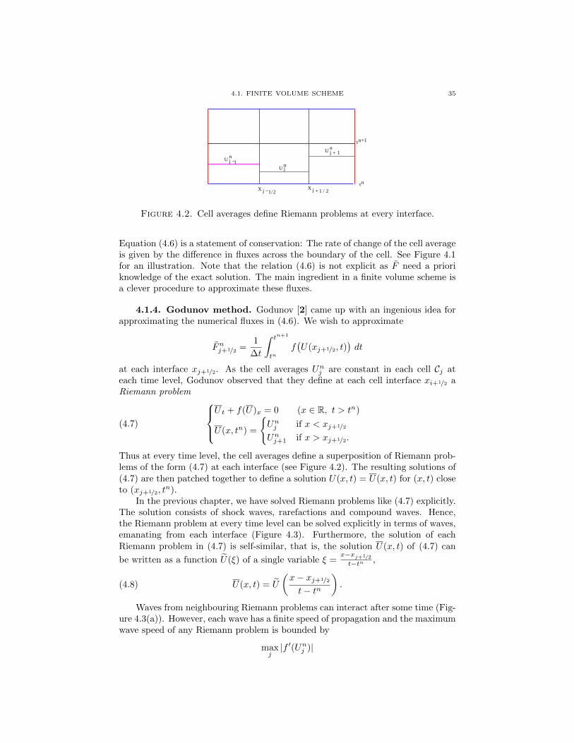
Figure 4.2. Cell averages define Riemann problems at every interface.
Equation (4.6) is a statement of conservation: The rate of change of the cell averageis given by the difference in fluxes across the boundary of the cell. See Figure 4.1for an illustration. Note that the relation (4.6) is not explicit as F need a prioriknowledge of the exact solution. The main ingredient in a finite volume scheme isa clever procedure to approximate these fluxes.
4.1.4. Godunov method. Godunov [2] came up with an ingenious idea forapproximating the numerical fluxes in (4.6). We wish to approximate
Fnj+1/2 =1
∆t
∫ tn+1
tnf(U(xj+1/2, t)
)dt
at each interface xj+1/2. As the cell averages Unj are constant in each cell Cj ateach time level, Godunov observed that they define at each cell interface xi+1/2 aRiemann problem
(4.7)
U t + f(U)x = 0 (x ∈ R, t > tn)
U(x, tn) =
Unj if x < xj+1/2
Unj+1 if x > xj+1/2.
Thus at every time level, the cell averages define a superposition of Riemann prob-lems of the form (4.7) at each interface (see Figure 4.2). The resulting solutions of(4.7) are then patched together to define a solution U(x, t) = U(x, t) for (x, t) closeto (xj+1/2, t
n).In the previous chapter, we have solved Riemann problems like (4.7) explicitly.
The solution consists of shock waves, rarefactions and compound waves. Hence,the Riemann problem at every time level can be solved explicitly in terms of waves,emanating from each interface (Figure 4.3). Furthermore, the solution of eachRiemann problem in (4.7) is self-similar, that is, the solution U(x, t) of (4.7) can
be written as a function U(ξ) of a single variable ξ =x−xj+1/2
t−tn ,
(4.8) U(x, t) = U
(x− xj+1/2
t− tn
).
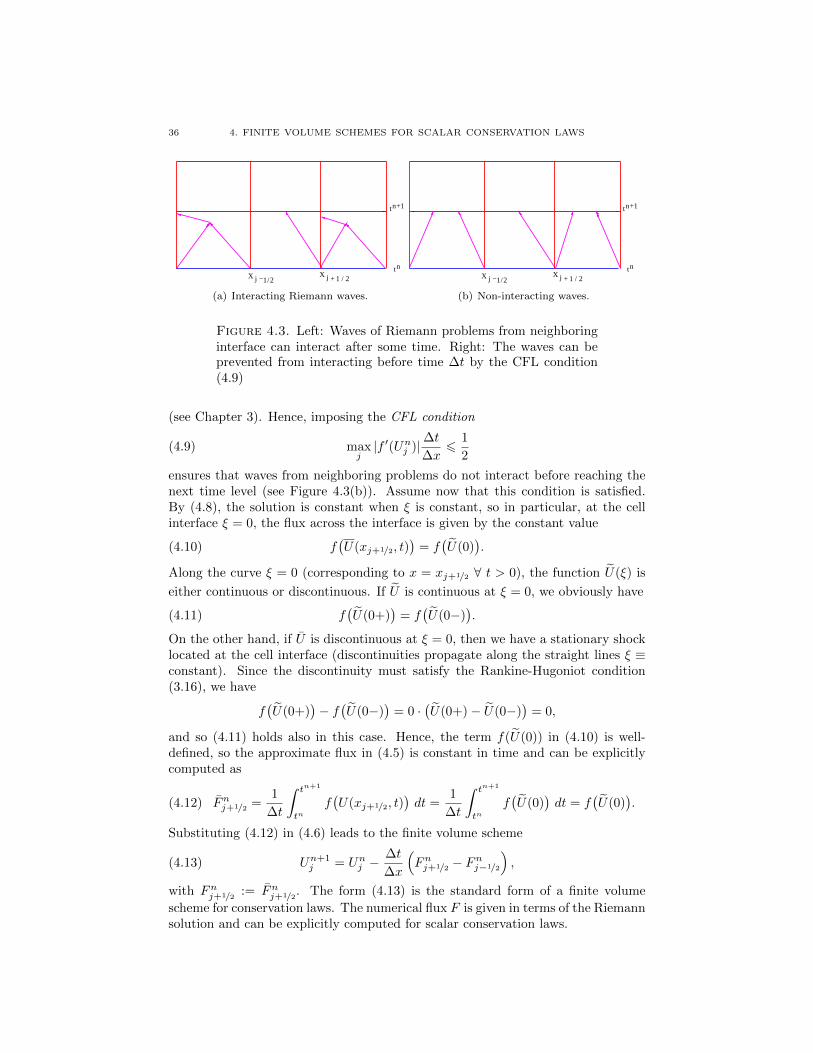
Waves from neighbouring Riemann problems can interact after some time (Fig-ure 4.3(a)). However, each wave has a finite speed of propagation and the maximumwave speed of any Riemann problem is bounded by
maxj|f ′(Unj )|
36 4. FINITE VOLUME SCHEMES FOR SCALAR CONSERVATION LAWS
X j −1/2X j + 1 / 2
tn
tn+1
(a) Interacting Riemann waves.
X j −1/2X j + 1 / 2
tn
tn+1
(b) Non-interacting waves.
Figure 4.3. Left: Waves of Riemann problems from neighboringinterface can interact after some time. Right: The waves can beprevented from interacting before time ∆t by the CFL condition(4.9)
(see Chapter 3). Hence, imposing the CFL condition
(4.9) maxj|f ′(Unj )|∆t
∆x6
1
2
ensures that waves from neighboring problems do not interact before reaching thenext time level (see Figure 4.3(b)). Assume now that this condition is satisfied.By (4.8), the solution is constant when ξ is constant, so in particular, at the cellinterface ξ = 0, the flux across the interface is given by the constant value
(4.10) f(U(xj+1/2, t)
)= f
(U(0)
).
Along the curve ξ = 0 (corresponding to x = xj+1/2 ∀ t > 0), the function U(ξ) is
either continuous or discontinuous. If U is continuous at ξ = 0, we obviously have
(4.11) f(U(0+)
)= f
(U(0−)
).
On the other hand, if U is discontinuous at ξ = 0, then we have a stationary shocklocated at the cell interface (discontinuities propagate along the straight lines ξ ≡constant). Since the discontinuity must satisfy the Rankine-Hugoniot condition(3.16), we have
f(U(0+)
)− f
(U(0−)
)= 0 ·
(U(0+)− U(0−)
)= 0,
and so (4.11) holds also in this case. Hence, the term f(U(0)) in (4.10) is well-defined, so the approximate flux in (4.5) is constant in time and can be explicitlycomputed as
(4.12) Fnj+1/2 =1
∆t
∫ tn+1
tnf(U(xj+1/2, t)
)dt =
1
∆t
∫ tn+1
tnf(U(0)
)dt = f
(U(0)
).
Substituting (4.12) in (4.6) leads to the finite volume scheme
(4.13) Un+1j = Unj −
∆t
∆x
(Fnj+1/2 − F
nj−1/2
),
with Fnj+1/2 := Fnj+1/2. The form (4.13) is the standard form of a finite volume
scheme for conservation laws. The numerical flux F is given in terms of the Riemannsolution and can be explicitly computed for scalar conservation laws.
4.1. FINITE VOLUME SCHEME 37
4.1.5. Godunov flux. It turns out that we can compute explicit formulas forthe numerical flux in (4.13). To this end, we need to obtain the value of the flux ofthe Riemann problem (4.7) at the interface xj+1/2. A lengthy computation basedon a case by case analysis leads to the formula
(4.14) Fnj+1/2 = F(Unj , U
n+1j
)=
min
Unj 6θ6Un
j+1
f(θ) if Unj 6 Unj+1
maxUn
j+16θ6Unj
f(θ) if Unj+1 6 Unj .
This formula is valid also for non-convex flux functions. The Godunov scheme is(4.13) with the Godunov flux (4.14).
Exercise 4.1. Computing the flux (4.14) can be complicated, since an optimizationproblem has to be solved. Show that in the special case where the flux function fhas a single minimum at the point ω and no local maxima, the formula (4.14) canbe simplified to
(4.15) Fnj+1/2 = F (Unj , Unj+1) = max
(f(max
(Unj , ω
)), f(min
(Unj+1, ω
))).
Note that strictly convex functions have this property. The formulas for the case ofa flux with a single maximum and no minima are obtained analogously.
Exercise 4.2. Show that for the linear transport equation (4.2), the Godunov scheme(4.13), (4.14) is identical to the standard upwind scheme (2.16). Thus, the Godunovscheme can be viewed as a generalization of the upwind scheme to nonlinear scalarconservation laws.
4.1.6. Numerical experiments. Consider Burgers’ equation (3.3) with Rie-mann data
(4.16) U(x, 0) =
1 if x < 0
0 if x > 0.
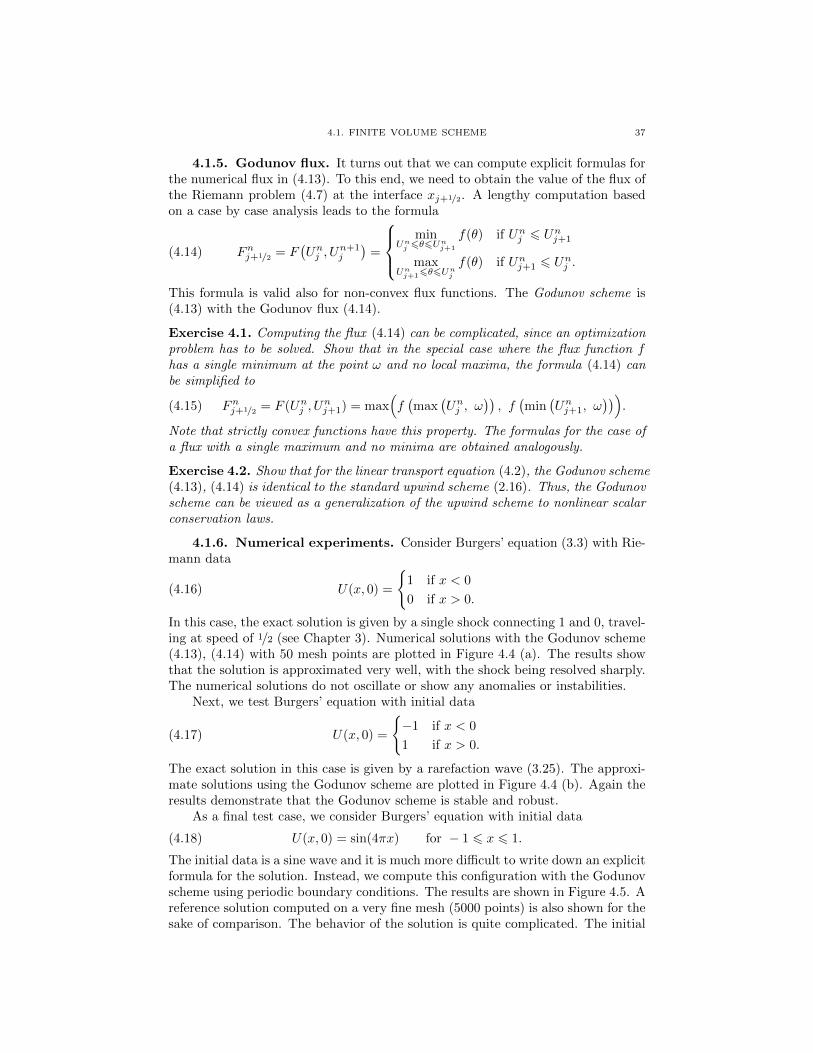
In this case, the exact solution is given by a single shock connecting 1 and 0, travel-ing at speed of 1/2 (see Chapter 3). Numerical solutions with the Godunov scheme(4.13), (4.14) with 50 mesh points are plotted in Figure 4.4 (a). The results showthat the solution is approximated very well, with the shock being resolved sharply.The numerical solutions do not oscillate or show any anomalies or instabilities.
Next, we test Burgers’ equation with initial data
(4.17) U(x, 0) =
−1 if x < 0
1 if x > 0.
The exact solution in this case is given by a rarefaction wave (3.25). The approxi-mate solutions using the Godunov scheme are plotted in Figure 4.4 (b). Again theresults demonstrate that the Godunov scheme is stable and robust.
As a final test case, we consider Burgers’ equation with initial data
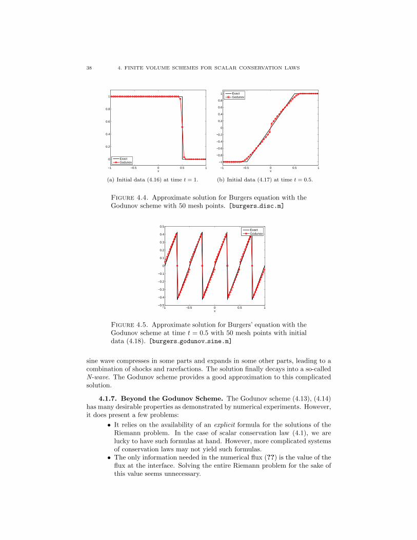
(4.18) U(x, 0) = sin(4πx) for − 1 6 x 6 1.
The initial data is a sine wave and it is much more difficult to write down an explicitformula for the solution. Instead, we compute this configuration with the Godunovscheme using periodic boundary conditions. The results are shown in Figure 4.5. Areference solution computed on a very fine mesh (5000 points) is also shown for thesake of comparison. The behavior of the solution is quite complicated. The initial
38 4. FINITE VOLUME SCHEMES FOR SCALAR CONSERVATION LAWS
−1 −0.5 0 0.5 1
0
0.2
0.4
0.6
0.8
1
x
ExactGodunov
(a) Initial data (4.16) at time t = 1.
−1 −0.5 0 0.5 1
−1
−0.8
−0.6
−0.4
−0.2
0
0.2
0.4
0.6
0.8
1
x
ExactGodunov
(b) Initial data (4.17) at time t = 0.5.
Figure 4.4. Approximate solution for Burgers equation with theGodunov scheme with 50 mesh points. [burgers disc.m]
−1 −0.5 0 0.5 1−0.5
−0.4
−0.3
−0.2
−0.1
0
0.1
0.2
0.3
0.4
0.5
x
ExactGodunov
Figure 4.5. Approximate solution for Burgers’ equation with theGodunov scheme at time t = 0.5 with 50 mesh points with initialdata (4.18). [burgers godunov sine.m]
sine wave compresses in some parts and expands in some other parts, leading to acombination of shocks and rarefactions. The solution finally decays into a so-calledN-wave. The Godunov scheme provides a good approximation to this complicatedsolution.
4.1.7. Beyond the Godunov Scheme. The Godunov scheme (4.13), (4.14)has many desirable properties as demonstrated by numerical experiments. However,it does present a few problems:
• It relies on the availability of an explicit formula for the solutions of theRiemann problem. In the case of scalar conservation law (4.1), we arelucky to have such formulas at hand. However, more complicated systemsof conservation laws may not yield such formulas.
• The only information needed in the numerical flux (??) is the value of theflux at the interface. Solving the entire Riemann problem for the sake ofthis value seems unnecessary.
4.2. APPROXIMATE RIEMANN SOLVERS 39
• At the level of implementation, the formula (4.15) provides a simple char-acterization of the Godunov flux for a large class of flux functions. How-ever, more complicated flux functions with a large number of extremalpoints need the solution of an optimization problem. Such a problemmight be very computationally costly.
These factors encourage the search for alternative numerical fluxes in (4.13).
4.2. Approximate Riemann Solvers
Since we are interested in approximating the solutions of the conservation law(4.1), it seems reasonable to replace the exact solutions of the Riemann problem(4.7) (used in the Godunov scheme) with approximate solutions. These approxi-mate solutions can then be used to define the numerical flux F as in (4.12). Suchschemes which replace the exact solutions of the Riemann problem (4.7) with ap-proximations called approximate Riemann solvers. We present some of them below.
4.2.1. Linearized (Roe) solvers. Our aim is to approximate the solutionsof the Riemann problem (4.7). A common method for solving nonlinear equationsis to linearize them. Linearization entails replacing the nonlinear flux function in(4.1) with a locally linearized version,
(4.19) f(U)x = f ′(U)Ux ≈ Aj+1/2Ux,
where A ≈ f ′ is a constant state around which the nonlinear flux function islinearized. There are many possible candidates for the linearizing state, one simplechoice being
Aj+1/2 = f ′(Unj + Unj+1
2
),
the flux of the arithmetic average of the two constant states. We will use a moresophisticated Roe average:
(4.20) Aj+1/2 =
f(Un
j+1)−f(Unj )
Unj+1−Un
jif Unj+1 6= Unj
f ′(Unj ) if Unj+1 = Unj .
Note that the Roe average also represents a linear approximation of f ′. The numer-ical flux F is obtained by replacing the Riemann problem (4.7) with a linearizedRiemann problem,
(4.21)
Ut + Aj+1/2Ux = 0
U(x, tn) =
Unj if x < xj+1/2
Unj+1 if x > xj+1/2.
This Riemann problem is very simple to solve as it involves a linear transportequation with a constant velocity field. Solving it explicitly we obtain the formula
(4.22) Fnj+1/2 = FRoe(Unj , U
nj+1
)=
f(Unj ) if Aj+1/2 > 0
f(Unj+1) if Aj+1/2 < 0.
The finite volume scheme (4.13) with the Roe flux (4.22) is termed the Roe orMurman-Roe scheme. It is simpler to implement when compared to the Godunovscheme as no optimization problem needs to be solved.
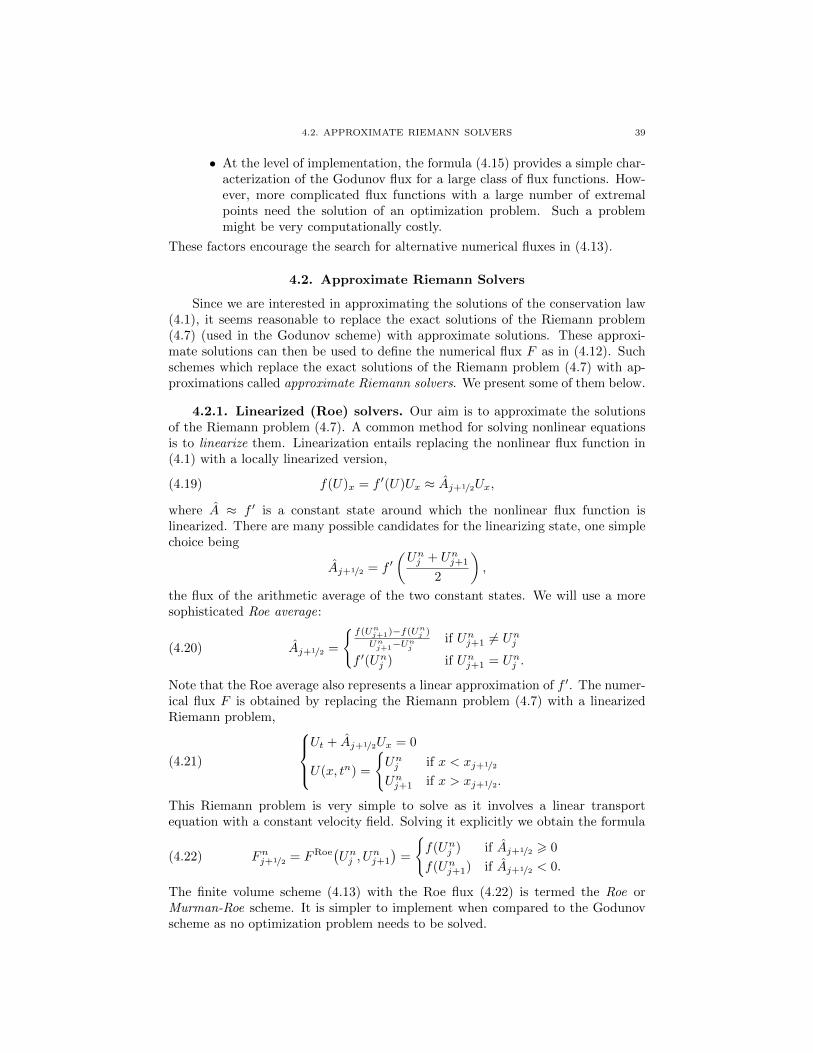
40 4. FINITE VOLUME SCHEMES FOR SCALAR CONSERVATION LAWS
Numerical results with the Roe scheme for Burgers’ equation with Riemanndata (4.16) are shown in Figure 4.6(a). They show that the Roe scheme approxi-mates the shock as accurately as the Godunov scheme.
Figure 4.6 (b) shows numerical results for the Riemann data (4.17). In thiscase, the Roe scheme fails completely and approximates the wrong stationary shocksolution. The same stationary solution persists even when the mesh is refined.Thus, the Roe scheme leads to numerical artifacts for some problems. This failurewill be analyzed in detail in the sequel.
−1 −0.5 0 0.5 1
0
0.2
0.4
0.6
0.8
1
x
ExactRoe
(a) Shock solution with initial data (4.16) att = 1.
−1 −0.5 0 0.5 1
−1
−0.8
−0.6
−0.4
−0.2
0
0.2
0.4
0.6
0.8
1
x
ExactRoe
(b) Rarefaction wave solution initial data(4.17) at t = 0.5.
Figure 4.6. Approximate solutions for Burgers equation with theRoe scheme with 50 mesh points. [burgers disc.m]
4.2.2. Central schemes. The Roe scheme fails at resolving rarefactions. Dueto linearization, the solution of the approximate Riemann problem (4.21) only con-sists of a single wave that travels to the right or to the left, depending on the sign ofthe Roe average A. When the exact solutions of Riemann problems for the conser-vation law consists of shocks, then the solution is a single, either left- or right-going,wave. However, the situation with rarefactions is very different. The rarefactionwave that solves (4.17) can travel in both directions (see Figure 4.7). As we haveseen, the Roe scheme may be unable to capture such behavior.
Unj
Unj + 1
U*j + 1/2
s lj + 1/2
s rj + 1/2
f *j + 1/2
Figure 4.7. An approximate Riemann solver with bi-directional waves.
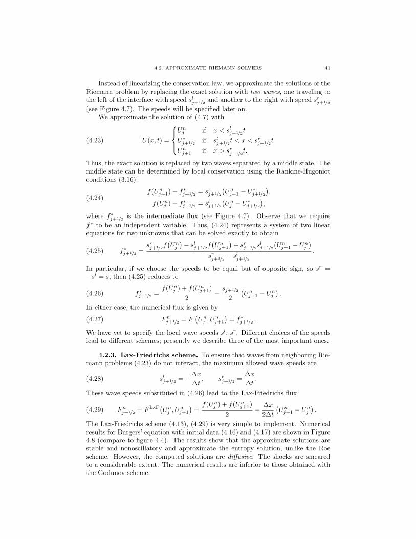
4.2. APPROXIMATE RIEMANN SOLVERS 41
Instead of linearizing the conservation law, we approximate the solutions of theRiemann problem by replacing the exact solution with two waves, one traveling tothe left of the interface with speed slj+1/2 and another to the right with speed srj+1/2
(see Figure 4.7). The speeds will be specified later on.We approximate the solution of (4.7) with
(4.23) U(x, t) =
Unj if x < slj+1/2t
U∗j+1/2 if slj+1/2t < x < srj+1/2t
Unj+1 if x > srj+1/2t.
Thus, the exact solution is replaced by two waves separated by a middle state. Themiddle state can be determined by local conservation using the Rankine-Hugoniotconditions (3.16):
(4.24)f(Unj+1)− f∗j+1/2 = srj+1/2
(Unj+1 − U∗j+1/2
),
f(Unj )− f∗j+1/2 = slj+1/2
(Unj − U∗j+1/2
),
where f∗j+1/2 is the intermediate flux (see Figure 4.7). Observe that we require
f∗ to be an independent variable. Thus, (4.24) represents a system of two linearequations for two unknowns that can be solved exactly to obtain
(4.25) f∗j+1/2 =srj+1/2f
(Unj)− slj+1/2f
(Unj+1
)+ srj+1/2s
lj+1/2
(Unj+1 − Unj
)srj+1/2 − s
lj+1/2
.
In particular, if we choose the speeds to be equal but of opposite sign, so sr =−sl = s, then (4.25) reduces to
(4.26) f∗j+1/2 =f(Unj ) + f(Unj+1)
2−sj+1/2
2
(Unj+1 − Unj
).
In either case, the numerical flux is given by
(4.27) Fnj+1/2 = F(Unj , U
nj+1
)= f∗j+1/2.
We have yet to specify the local wave speeds sl, sr. Different choices of the speedslead to different schemes; presently we describe three of the most important ones.
4.2.3. Lax-Friedrichs scheme. To ensure that waves from neighboring Rie-mann problems (4.23) do not interact, the maximum allowed wave speeds are
(4.28) slj+1/2 = −∆x
∆t, srj+1/2 =
∆x
∆t.
These wave speeds substituted in (4.26) lead to the Lax-Friedrichs flux
(4.29) Fnj+1/2 = FLxF(Unj , U
nj+1
)=f(Unj ) + f(Unj+1)
2− ∆x
2∆t
(Unj+1 − Unj
).
The Lax-Friedrichs scheme (4.13), (4.29) is very simple to implement. Numericalresults for Burgers’ equation with initial data (4.16) and (4.17) are shown in Figure4.8 (compare to figure 4.4). The results show that the approximate solutions arestable and nonoscillatory and approximate the entropy solution, unlike the Roescheme. However, the computed solutions are diffusive. The shocks are smearedto a considerable extent. The numerical results are inferior to those obtained withthe Godunov scheme.
42 4. FINITE VOLUME SCHEMES FOR SCALAR CONSERVATION LAWS
−1 −0.5 0 0.5 1
0
0.2
0.4
0.6
0.8
1
x
ExactLax−Friedrichs
(a) Shock solution with initial data (4.16) att = 1.
−1 −0.5 0 0.5 1
−1
−0.8
−0.6
−0.4
−0.2
0
0.2
0.4
0.6
0.8
1
x
ExactLax−Friedrichs
(b) Rarefaction wave solution with initial data(4.17) at t = 0.5.
Figure 4.8. Approximate solution for Burgers’ equation with theLax-Friedrichs scheme with 50 mesh points. [burgers disc.m]
4.2.4. Rusanov scheme. The Lax-Friedrichs scheme was quite diffusive aroundshocks. A possible explanation lies in the choice of the wave speeds (4.28). Thesespeeds were the maximum allowed speeds and did not take into the account thespeeds of propagation of the problem under consideration. A better, locally selected,choice of speeds is given by
(4.30) srj+1/2 = sj+1/2, slj+1/2 = −sj+1/2,
where
sj+1/2 = max(|f ′(Unj )|, |f ′(Unj+1)|
).
The resulting flux (4.26), called the Rusanov (or Local Lax-Friedrichs) flux, is givenby
Fnj+1/2 = FRus(Unj , U
nj+1
)=f(Unj ) + f(Unj+1)
2−
max(|f ′(Unj )|, |f ′(Unj+1)|
)2
(Unj+1 − Unj
).
(4.31)
The Rusanov scheme (4.13), (4.31) leads to a considerable improvement in resultsover the Lax-Friedrichs scheme, as shown in Figure 4.9.
4.2.5. Engquist-Osher scheme. A related scheme is the Engquist-Osherscheme, which has flux
Fnj+1/2 = FEO(Unj , U
nj+1
)=f(Unj ) + f(Unj+1)
2− 1
2
∫ Unj+1
Unj
|f ′(θ)| dθ.(4.32)
Although it is difficult to write the Engquist-Osher flux as an approximate Riemannsolver, it shares several features of approximate Riemann solvers. When the fluxfunction has a single minimum at a point ω and no maxima (which is the case formost convex functions), the Engquist-Osher flux can be explicitly computed as
(4.33) FEO(Unj , U
nj+1
)= f
(max
(Unj , ω
))+ f
(min
(Unj+1, ω
))− f(ω).
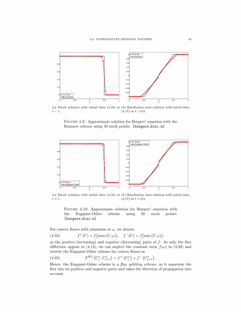
4.2. APPROXIMATE RIEMANN SOLVERS 43
−1 −0.5 0 0.5 1
0
0.2
0.4
0.6
0.8
1
x
ExactRusanov
(a) Shock solution with initial data (4.16) att = 1.
−1 −0.5 0 0.5 1
−1
−0.8
−0.6
−0.4
−0.2
0
0.2
0.4
0.6
0.8
1
x
ExactRusanov
(b) Rarefaction wave solution with initial data(4.17) at t = 0.5.
Figure 4.9. Approximate solution for Burgers’ equation with theRusanov scheme using 50 mesh points. [burgers disc.m]
−1 −0.5 0 0.5 1
0
0.2
0.4
0.6
0.8
1
x
ExactEngquist−Osher
(a) Shock solution with initial data (4.16) att = 1.
−1 −0.5 0 0.5 1
−1
−0.8
−0.6
−0.4
−0.2
0
0.2
0.4
0.6
0.8
1
x
ExactEngquist−Osher
(b) Rarefaction wave solution with initial data(4.17) at t = 0.5.
Figure 4.10. Approximate solution for Burgers’ equation withthe Engquist-Osher scheme using 50 mesh points.[burgers disc.m]
For convex fluxes with minimum at ω, we denote
(4.34) f+(U) = f(max (U, ω)
), f−(U) = f
(min (U, ω)
),
as the positive (increasing) and negative (decreasing) parts of f . As only the fluxdifference appear in (4.13), we can neglect the constant term f(ω) in (4.33) andrewrite the Engquist-Osher scheme for convex fluxes as
(4.35) FEO(Unj , U
nj+1
)= f+
(Unj)
+ f−(Unj+1
).
Hence, the Engquist-Osher scheme is a flux splitting scheme, as it separates theflux into its positive and negative parts and takes the direction of propagation intoaccount.
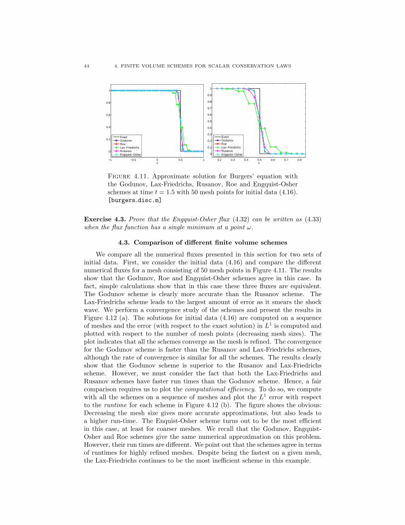
44 4. FINITE VOLUME SCHEMES FOR SCALAR CONSERVATION LAWS
−1 −0.5 0 0.5 1
0
0.2
0.4
0.6
0.8
1
x
ExactGodunovRoeLax−FriedrichsRusanovEngquist−Osher
0.2 0.3 0.4 0.5 0.6 0.7 0.8
0
0.1
0.2
0.3
0.4
0.5
0.6
0.7
0.8
0.9
1
x
ExactGodunovRoeLax−FriedrichsRusanovEngquist−Osher
Figure 4.11. Approximate solution for Burgers’ equation withthe Godunov, Lax-Friedrichs, Rusanov, Roe and Engquist-Osherschemes at time t = 1.5 with 50 mesh points for initial data (4.16).[burgers disc.m]
Exercise 4.3. Prove that the Engquist-Osher flux (4.32) can be written as (4.33)when the flux function has a single minimum at a point ω.
4.3. Comparison of different finite volume schemes
We compare all the numerical fluxes presented in this section for two sets ofinitial data. First, we consider the initial data (4.16) and compare the differentnumerical fluxes for a mesh consisting of 50 mesh points in Figure 4.11. The resultsshow that the Godunov, Roe and Engquist-Osher schemes agree in this case. Infact, simple calculations show that in this case these three fluxes are equivalent.The Godunov scheme is clearly more accurate than the Rusanov scheme. TheLax-Friedrichs scheme leads to the largest amount of error as it smears the shockwave. We perform a convergence study of the schemes and present the results inFigure 4.12 (a). The solutions for initial data (4.16) are computed on a sequenceof meshes and the error (with respect to the exact solution) in L1 is computed andplotted with respect to the number of mesh points (decreasing mesh sizes). Theplot indicates that all the schemes converge as the mesh is refined. The convergencefor the Godunov scheme is faster than the Rusanov and Lax-Friedrichs schemes,although the rate of convergence is similar for all the schemes. The results clearlyshow that the Godunov scheme is superior to the Rusanov and Lax-Friedrichsscheme. However, we must consider the fact that both the Lax-Friedrichs andRusanov schemes have faster run times than the Godunov scheme. Hence, a faircomparison requires us to plot the computational efficiency. To do so, we computewith all the schemes on a sequence of meshes and plot the L1 error with respectto the runtime for each scheme in Figure 4.12 (b). The figure shows the obvious:Decreasing the mesh size gives more accurate approximations, but also leads toa higher run-time. The Enquist-Osher scheme turns out to be the most efficientin this case, at least for coarser meshes. We recall that the Godunov, Engquist-Osher and Roe schemes give the same numerical approximation on this problem.However, their run times are different. We point out that the schemes agree in termsof runtimes for highly refined meshes. Despite being the fastest on a given mesh,the Lax-Friedrichs continues to be the most inefficient scheme in this example.
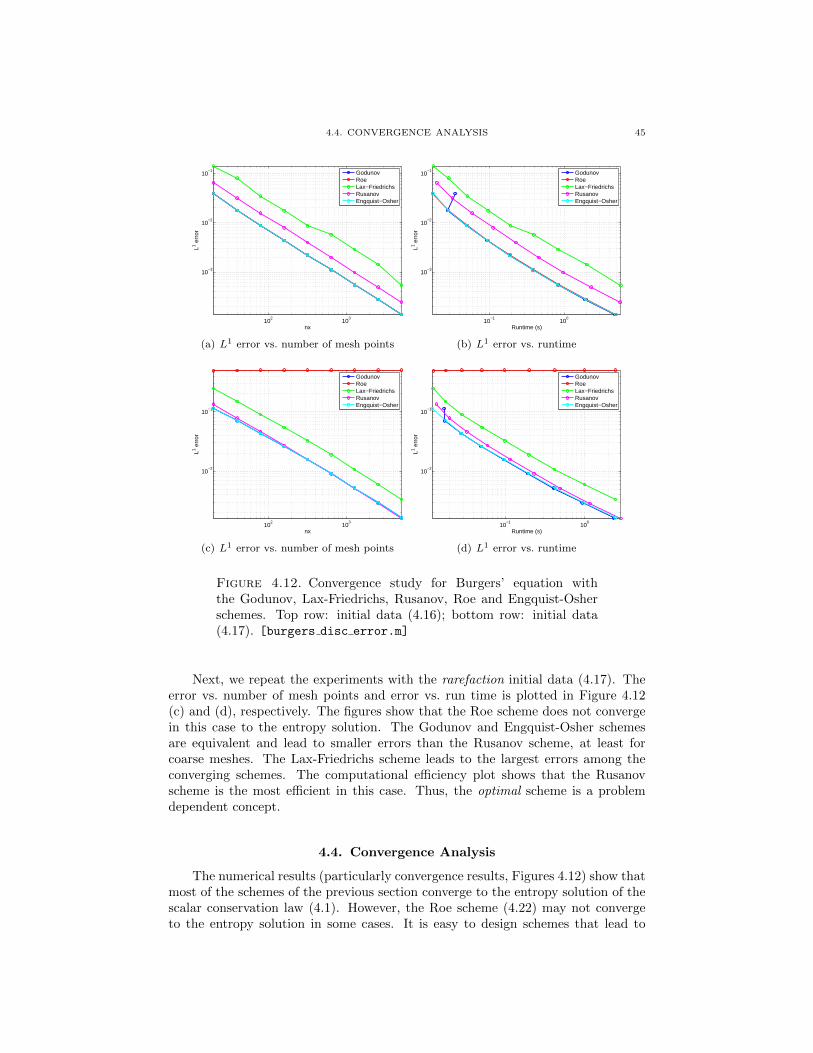
4.4. CONVERGENCE ANALYSIS 45
102
103
10−3
10−2
10−1
nx
L1 err
or
GodunovRoeLax−FriedrichsRusanovEngquist−Osher
(a) L1 error vs. number of mesh points
10−1
100
10−3
10−2
10−1
Runtime (s)
L1 err
or
GodunovRoeLax−FriedrichsRusanovEngquist−Osher
(b) L1 error vs. runtime
102
103
10−2
10−1
nx
L1 err
or
GodunovRoeLax−FriedrichsRusanovEngquist−Osher
(c) L1 error vs. number of mesh points
10−1
100
10−2
10−1
Runtime (s)
L1 err
or
GodunovRoeLax−FriedrichsRusanovEngquist−Osher
(d) L1 error vs. runtime
Figure 4.12. Convergence study for Burgers’ equation withthe Godunov, Lax-Friedrichs, Rusanov, Roe and Engquist-Osherschemes. Top row: initial data (4.16); bottom row: initial data(4.17). [burgers disc error.m]
Next, we repeat the experiments with the rarefaction initial data (4.17). Theerror vs. number of mesh points and error vs. run time is plotted in Figure 4.12(c) and (d), respectively. The figures show that the Roe scheme does not convergein this case to the entropy solution. The Godunov and Engquist-Osher schemesare equivalent and lead to smaller errors than the Rusanov scheme, at least forcoarse meshes. The Lax-Friedrichs scheme leads to the largest errors among theconverging schemes. The computational efficiency plot shows that the Rusanovscheme is the most efficient in this case. Thus, the optimal scheme is a problemdependent concept.
4.4. Convergence Analysis
The numerical results (particularly convergence results, Figures 4.12) show thatmost of the schemes of the previous section converge to the entropy solution of thescalar conservation law (4.1). However, the Roe scheme (4.22) may not convergeto the entropy solution in some cases. It is easy to design schemes that lead to
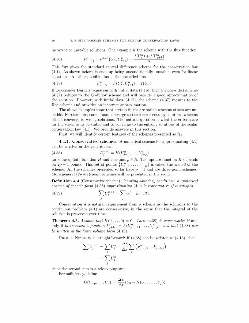
46 4. FINITE VOLUME SCHEMES FOR SCALAR CONSERVATION LAWS
incorrect or unstable solutions. One example is the scheme with the flux function
(4.36) Fnj+1/2 = FCen(Unj , U
nj+1
)=f(Unj ) + f(Unj+1)
2.
This flux gives the standard central difference scheme for the conservation law(4.1). As shown before, it ends up being unconditionally unstable, even for linearequations. Another possible flux is the one-sided flux
(4.37) Fnj+1/2 = F (Unj , Unj+1) = f(Unj ).
If we consider Burgers’ equation with initial data (4.16), then the one-sided scheme(4.37) reduces to the Godunov scheme and will provide a good approximation ofthe solution. However, with initial data (4.17), the scheme (4.37) reduces to theRoe scheme and provides an incorrect approximation.
The above examples show that certain fluxes are stable whereas others are un-stable. Furthermore, some fluxes converge to the correct entropy solutions whereasothers converge to wrong solutions. The natural question is what the criteria arefor the schemes to be stable and to converge to the entropy solutions of the scalarconservation law (4.1). We provide answers in this section.
First, we will identify certain features of the schemes presented so far.
4.4.1. Conservative schemes. A numerical scheme for approximating (4.1)can be written in the generic form
(4.38) Un+1j = H
(Unj−p, . . . , U
nj+p
)for some update function H and constant p ∈ N. The update function H dependson 2p + 1 points. This set of points
Unj−p, . . . , U
nj+p
is called the stencil of the
scheme. All the schemes presented so far have p = 1 and are three-point schemes.More general (2p+ 1)-point schemes will be presented in the sequel.
Definition 4.4 (Conservative scheme). Ignoring boundary conditions, a numericalscheme of generic form (4.38) approximating (4.1) is conservative if it satisfies
(4.39)∑j
Un+1j =
∑j
Unj for all n.
Conservation is a natural requirement from a scheme as the solutions to thecontinuous problem (4.1) are conservative, in the sense that the integral of thesolution is preserved over time.
Theorem 4.5. Assume that H(0, . . . , 0) = 0. Then (4.38) is conservative if andonly if there exists a function Fnj+1/2 = F (Unj−p+1, . . . , U
nj+p) such that (4.38) can
be written in the finite volume form (4.13).
Proof. Necessity is straightforward: if (4.38) can be written as (4.13), then∑j
Un+1j =
∑j
Unj −∆t
∆x
∑j
(Fnj+1/2 − F
nj−1/2
)=∑j
Unj ,
since the second sum is a telescoping sum.For sufficiency, define
G(U−p, . . . , Up) :=∆x
∆t(U0 −H(U−p, . . . , Up))
4.4. CONVERGENCE ANALYSIS 47
(we drop the time dependence for the moment). By conservation, we have∑j
G(Uj−p, . . . , Uj+p) = 0.
We want to show that there is an Fj+1/2 = F (Uj−p+1, Uj+p) such that
(4.40) Fj+1/2 − Fj−1/2 = G(Uj−p, . . . , Uj+p).
If will suffice to construct Fj+1/2 for j = 0. Select first Uj such that Uj = 0 wheneverj 6 −p or j > p. Then
0 =∑j
G(Uj−p, . . . , Uj+p)
= G(0, . . . , 0, U−p+1) + · · ·+G(0, U−p+1, . . . , Up)
+G(U−p+1, . . . , Up, 0) + · · ·+G(Up, 0, . . . , 0)
= F1/2 +B
where we have defined F1/2 := G(0, . . . , 0, U−p+1) + · · · + G(0, U−p+1, . . . , Up) andB := G(U−p+1, . . . , Up, 0) + · · ·+G(Up, 0, . . . , 0). Next, select Uj such that Uj = 0whenever j < −p or j > p. Then
0 =∑j
G(Uj−p, . . . , Uj+p)
= G(0, . . . , 0, U−p) + · · ·+G(0, U−p, . . . , Up−1) +G(U−p, . . . , Up)
+G(U−p+1, . . . , Up, 0) + · · ·+G(Up, 0, . . . , 0)
= F−1/2 +G(U−p, . . . , Up) +B.
Subtracting these two identities, we get the desired identity (4.40).
The definition of conservation needs to be modified when boundaries are in-cluded in the discussion.
4.4.2. Consistent schemes. Another crucial requirement is consistency. Letsome (2p+ 1)-point scheme (4.38) be given with numerical flux
(4.41) Fnj+1/2 = F (Unj−p+1, . . . , Unj+p).
Definition 4.6 (Consistency). A finite volume scheme (4.13) with numerical fluxfunction (4.41) is consistent if
(4.42) F (U, . . . , U) = f(U) for all U ∈ R.
It is straightforward to check that all the two-point numerical flux functionspresented so far are consistent. Consistency is a natural requirement to ensure thatthe scheme approximates the correct conservation law.
Conservation and consistency are shared by all the schemes discussed till now.However, these criteria do not ensure either stability or convergence; for instance,the central scheme (4.36) is both consistent and conservative, but fails to be stable.Similarly, the Roe scheme (4.22) is consistent and conservative, but does not con-verge to the entropy solution in certain numerical experiments. We need anothercriterion.
48 4. FINITE VOLUME SCHEMES FOR SCALAR CONSERVATION LAWS
4.4.3. Monotone schemes. The entropy solutions of (4.1) are monotonicitypreserving, meaning that if U and V are entropy solutions of (4.1) with initial dataU0 and V0, respectively, then
U0(x) 6 V0(x) for all x ⇒ U(x, t) 6 V (x, t) for all x, t.
It is desirable for numerical schemes to posses this property. At the discrete level,it is defined by the following.
Definition 4.7. A numerical scheme (4.38) is monotone if the update function His non-decreasing in each of its arguments.
If (4.38) can be written in the finite volume form (4.13) with a two-point fluxfunction (so p = 1 in (4.41)), then a sufficient condition for monotonicity is givenby
Lemma 4.8. A finite volume scheme (4.13) with a two-point flux F = F (a, b) ismonotone if F is a Lipschitz continuous function in both arguments, non-decreasingin its first argument and non-increasing in its second argument. More specifically,the following hold:
(4.43)a 7→ F (a, b) is non-decreasing for fixed b,
b 7→ F (a, b) is non-increasing for fixed a,
and the following CFL-type condition holds:
(4.44)
∣∣∣∣∂F∂a∣∣∣∣+
∣∣∣∣∂F∂b∣∣∣∣ 6 ∆x
∆t.
The proof of this lemma is left as an exercise to the reader.
4.4.4. Examples of monotone schemes. Assume that the flux function fin (4.1) is a differentiable function. Then the following schemes are monotone:
• The Lax-Friedrichs scheme (4.29) has a smooth C1 numerical flux func-tion. Explicit computations result in
∂F
∂a=
1
2
(f ′(a) +
∆x
∆t
)∂F
∂b=
1
2
(f ′(b)− ∆x
∆t
).
The condition (4.44) then follows from the CFL condition (4.9).• The Rusanov scheme (4.31) is monotone. The proof follows as above.• The Engquist-Osher scheme (4.32) has a smooth numerical flux. A direct
calculation shows that
∂F
∂a=
1
2(f ′(a) + |f ′(a)|)
∂F
∂a=
1
2(f ′(b)− |f ′(b)|) .
Furthermore, the CFL condition (4.44) is a consequence of (4.9). Hence,the Engquist-Osher scheme is monotone.
• The Godunov scheme (4.14) has a Lipschitz continuous flux function. It iscumbersome to check by a case by case analysis that the Godunov schemeis monotone. A heuristic explanation relies on the fact that the both
4.4. CONVERGENCE ANALYSIS 49
the evolution and averaging operators used in the deriving the Godunovscheme are monotone operators.
On the other hand, it is easy to check that the central flux (4.36), the one-sided flux(4.37) and the Roe flux (4.22) are not monotone. Thus, monotonicity of the schemeprovides a demarcation between robust and potentially non-robust schemes.
4.4.5. Stability estimates. The numerical experiments indicate that mono-tone schemes are stable and converge to the entropy solution, whereas the non-monotone schemes may be unstable or may converge to the incorrect solution. Acrucial step in proving convergence is to obtain stability estimates on the approxi-mate solutions, computed by the schemes.
From our study of the continuous problem in the previous section, the entropysolutions of the continuous problem (4.1) satisfy the following stability estimates.
(i) L∞ estimate (3.38) as a consequence of a maximum principle.(ii) Lp estimates (3.30) for 1 6 p < ∞ as a consequence of the entropy
inequality (3.29).(iii) The BV estimate (3.39) showing that the solutions are TVD.
The central philosophy of numerical analysis is to device numerical schemes thatpreserve stability properties of the underlying continuous problem. Hence, it isnatural to examine whether the finite volume schemes presented in this sectionsatisfy discrete versions of the above stability estimates.
L∞ bounds. A consistent three point finite volume scheme (4.13) can be writ-ten as
(4.45) Un+1j = H(Unj−1, U
nj , U
nj+1),
with the consistency of the fluxes F in (4.13) implying that
H(U,U, U) = U.
The scheme (4.45) is monotone if H is non-decreasing in each of its three arguments.The Godunov, Engquist-Osher, Lax-Friedrichs and Rusanov schemes (under a CFLcondition like (4.9)) are examples of three-point monotone schemes. These schemessatisfy the following discrete maximum principle.
Lemma 4.9. Let Unj be the approximate solutions generated by a three-point con-sistent monotone scheme of the form (4.45). Then the solutions satisfy
(4.46) min(Unj−1, U
nj , U
nj+1
)6 Un+1
j 6 max(Unj−1, U
nj , U
nj+1
)for all n, j.
In particular, we have
(4.47) minkU0k 6 U
nj 6 max
kU0k for all n, j.
Proof. Let Unj = max(Unj−1, U
nj , U
nj+1
). By definition,
Unj−1, Unj , U
nj+1 6 U
nj .
Since the scheme (4.45) is monotone, the update function H is monotone non-decreasing in each of its arguments. Therefore
Un+1j = H(Unj−1, U
nj , U
nj+1) 6 H(Unj , U
nj , U
nj+1) (monotonicity)
6 H(Unj , Unj , U
nj+1) (monotonicity)
6 H(Unj , Unj , U
nj ) (monotonicity)
50 4. FINITE VOLUME SCHEMES FOR SCALAR CONSERVATION LAWS
= Unj (consistency).
The minimum principle follows analogously. Iterating the maximum principle (4.46)over all time levels up to n yields the L∞ bound (4.47).
4.4.6. Entropy inequalities and Lp bounds. The key to obtaining Lp
bounds and characterizing the correct entropy solution is to obtain a discrete ver-sion of the entropy inequality (3.29). As we have seen in Chapter 3, it is enough toobtain a discrete version of the Kruzkhov entropy inequality (3.33). We proceed todo so below.
For a constant k ∈ R, define the Crandall-Majda numerical entropy flux as
Qnj+1/2 = Q(Unj , Unj+1)
= F (Unj ∨ k, Unj+1 ∨ k)− F (Unj ∧ k, Unj+1 ∧ k),(4.48)
where we use the notation
a ∨ b = max(a, b), a ∧ b = min(a, b).
Note that this numerical entropy flux is consistent with (3.32) whenever the nu-merical flux F is consistent, as
Q(U,U) = F (U ∨ k, U ∨ k)− F (U ∧ k, U ∧ k)
= f(U ∨ k)− f(U ∧ k)
= sign(U − k)(f(U)− f(k))
= Q(U, k).
In the following lemma we obtain a discrete version of (3.33).
Lemma 4.10 (Crandall-Majda). Let Unj be an approximate solution computed bya consistent and monotone three-point scheme (4.45). Then U satisfies the discreteentropy inequality
(4.49) |Un+1j − k| − |Unj − k|+
∆t
∆x
(Qnj+1/2 −Q
nj−1/2
)6 0
for all n, j.
Proof. By definition of the scheme (4.45) and (4.13), we have
H(Unj−1 ∨ k, Unj ∨ k, Unj+1 ∨ k
)= Unj ∨ k −
∆t
∆x
(F(Unj ∨ k, Unj+1 ∨ k
)− F
(Unj−1 ∨ k, Unj ∨ k
))and
H(Unj−1 ∧ k, Unj ∧ k, Unj+1 ∧ k
)= Unj ∧ k −
∆t
∆x
(F(Unj ∧ k, Unj+1 ∧ k
)− F
(Unj−1 ∧ k, Unj ∧ k
)).
Using the definition of Qnj+1/2, we obtain
(4.50)
H(Unj−1 ∨ k, Unj ∨ k, Unj+1 ∨ k
)−H
(Unj−1 ∧ k, Unj ∧ k, Unj+1 ∧ k
)= Unj ∨ k − Unj ∧ k −
∆t
∆x
(Qnj+1/2 −Q
nj−1/2
)= |Unj − k| −
∆t
∆x
(Qnj+1/2 −Q
nj−1/2
).
4.4. CONVERGENCE ANALYSIS 51
By monotonicity and the definition of H (4.45),
(4.51)H(Unj−1 ∨ k, Unj ∨ k, Unj+1 ∨ k
)> H
(Unj−1, U
nj , U
nj+1
)= Un+1
j ,
H(Unj−1 ∧ k, Unj ∧ k, Unj+1 ∧ k
)6 H
(Unj−1, U
nj , U
nj+1
)= Un+1
j .
Similarly, by monotonicity and consistency of H,
(4.52)H(Unj−1 ∨ k, Unj ∨ k, Unj+1 ∨ k
)> H(k, k, k) = k,
H(Unj−1 ∧ k, Unj ∧ k, Unj+1 ∧ k
)6 H(k, k, k) = k.
By subtracting (4.52) from (4.51) and using (4.50), we obtain
|Unj − k| −∆t
∆x
(Qnj+1/2 −Q
nj−1/2
)> |Un+1
j − k|,
which proves (4.49).
Remark 4.11. The discrete entropy inequality (4.49) can be used with an approxi-mation argument for Kruzkhov entropies (3.31) to obtain discrete entropy inequali-ties for any convex function S. This implies Lp bounds on the solution by summingover all mesh points.
4.4.7. TV bounds. Another essential stability estimate for scalar conserva-tion laws (4.1) is the BV estimate (3.39), which provides control over the oscillationsin the solution. This estimate says that the entropy solutions of (4.1) are TVD,meaning that the TV norm does not increase in time. We need to obtain a discreteversion of this total variation. The total variation of a piecewise constant functionat time level tn is given by ∑
j
|Unj+1 − Unj |.
The first step for obtaining a TV bound is rewriting the finite volume schemein the incremental form
(4.53) Un+1j = Unj + Cnj+1/2
(Unj+1 − Unj
)−Dn
j−1/2
(Unj − Unj−1
)with incremental coefficients
(4.54) Cnj+1/2 =∆t
∆x
f(Unj )− Fnj+1/2
Unj+1 − Unj, Dn
j+1/2 =∆t
∆x
f(Unj+1)− Fnj+1/2
Unj+1 − Unj.
A straightforward calculation shows that the incremental form (4.53) is equivalentto the standard finite volume form (4.13). The advantage of the incremental formlies in the following useful lemma.
Lemma 4.12 (Harten’s Lemma). Assume that the scheme (4.53) satisfies
(4.55) Cnj+1/2, Dnj+1/2 > 0 and Cnj+1/2 +Dn
j+1/2 6 1 for all n, j.
Then solutions computed with (4.53) are TVD, i.e. they satisfy
(4.56)∑j
|Un+1j+1 − U
n+1j | 6
∑j
|Unj+1 − Unj |.
Proof. Using the incremental form (4.53), we obtain
Un+1j+1 − U
n+1j =
(1− Cnj+1/2 −D
nj+1/2
)(Unj+1 − Unj
)+ Cnj+3/2
(Unj+2 − Unj+1
)+Dn
j−1/2
(Unj − Unj−1
).
52 4. FINITE VOLUME SCHEMES FOR SCALAR CONSERVATION LAWS
Taking absolute values on both sides of the above equation and using (4.55) yields∣∣Un+1j+1 − U
n+1j
∣∣ =(
1− Cnj+1/2 −Dnj+1/2
) ∣∣Unj+1 − Unj∣∣
+ Cnj+3/2
∣∣Unj+2 − Unj+1
∣∣+Dnj−1/2
∣∣Unj − Unj−1
∣∣ .Summing over j and identifying equal terms, we obtain the TVD estimate (4.56).
Harten’s lemma allows us to check whether a scheme in incremental form isTVD or not. It turns out that consistent monotone schemes are TVD.
Lemma 4.13. Any consistent monotone three-point finite volume scheme (4.13) isTVD under the CFL condition (4.44).
Proof. We need to check if the scheme satisfies the conditions (4.55) of Harten’slemma. By explicit computations we obtain
Cnj+1/2 =∆t
∆x
f(Unj )− F (Unj , Unj+1)
Unj+1 − Unj(definition (4.54))
=∆t
∆x
F (Unj , Unj )− F (Unj , U
nj+1)
Unj+1 − Unj(consistency)
> 0 (monotonicity).
The correct sign of D can be similarly checked. We also have
Cnj+1/2 =∆t
∆x
f(Unj )− F (Unj , Unj+1)
Unj+1 − Unj(definition (4.54))
=∆t
∆x
F (Unj , Unj )− F (Unj , U
nj+1)
Unj+1 − Unj(consistency)
6∆t
∆x
∣∣∣∣∂F∂b∣∣∣∣ (Lipschitz flux).
Similarly,
Dnj+1/2 6
∆t
∆x
∣∣∣∣∂F∂a∣∣∣∣ .
Therefore,
1− Cnj+1/2 −Dnj+1/2 > 1− ∆t
∆x
(∣∣∣∣∂F∂b∣∣∣∣+
∣∣∣∣∂F∂a∣∣∣∣)
> 0
by the CFL condition (4.44).
4.4.8. Convergence result. In the previous sections, we have establishedthat monotone consistent conservative schemes are stable in L∞, are TVD andsatisfy a discrete entropy condition (4.49). These stability estimates pave the wayfor showing that the approximate solutions computed by any monotone consistentconservative scheme converge to the entropy solution of (4.1). The following famoustheorem, due to Lax and Wendroff, says that if the approximate solutions Unjcomputed by a consistent and conservative scheme converge, then the limit is a
4.4. CONVERGENCE ANALYSIS 53
weak solution of the conservation law. For ease of notation, we will identify theapproximate solutions with a piecewise constant function,
(4.57) U∆(x, t) = Unj for (x, t) ∈ [xj−1/2, xj+1/2)× [tn, tn+1).
Theorem 4.14 (Lax-Wendroff). Let Unj be approximate solutions of (4.1), com-puted by a conservative and consistent finite volume scheme (4.13) with a differen-tiable (or Lipschitz) numerical flux function F . Assume that U0 ∈ L∞(R) and thatthe approximating functions U∆
• are uniformly bounded, i.e,
(4.58) ‖U∆‖L∞(R×R+) 6 C
for some constant C > 0;• converge to some function U in L1(R× R+) and almost everywhere.
Then U is a weak solution of (4.1)
Proof. Let φ ∈ C∞c (R × [0,∞)) be a given test function and denote φnj =φ(xj , t
n). By multiplying (4.13) by ∆xφnj and summing over j ∈ Z and n ∈ N0, weobtain
0 = ∆x∆t
∞∑j=−∞
∞∑n=0
(Un+1j − Unj
∆t+Fnj+1/2 − F
nj−1/2
∆x
)φnj
(summation by parts)
= −∆x
∞∑j=−∞
U0j φ
0j −∆x∆t
∞∑j=−∞
∞∑n=0
(Un+1j
φn+1j − φnj
∆t+ Fnj+1/2
φnj+1 − φnj∆x
).
Note that since φ has compact support, only finitely many of the summands in theabove expression are nonzero, and so all the sums are well-defined. As with U∆,define φ∆(x, t) = φnj for (x, t) ∈ [xj−1/2, xj+1/2)× [tn, tn+1). Recognizing the aboveexpression as a Riemann sum of step functions, it can be written as
∫RU∆(x, 0)φ∆(x, 0) dx+
∫R
∫ ∞0
U∆(x, t+ ∆t)φ∆(x, t+ ∆t)− φ∆(x, t)
∆tdtdx
+
∫R
∫ ∞0
F(U∆(x, t), U∆(x+ ∆x, t)
) φ∆(x+ ∆x, t)− φ∆(x, t)
∆xdtdx = 0.
(4.59)
Both U∆ and φ∆ converge boundedly a.e. to U and φ, respectively, so by Lebesgue’sdominated convergence theorem, the first two terms converge to∫
RU(x, 0)φ(x, 0) dx+
∫R
∫ ∞0
U(x, t)φt(x, t) dtdx
as ∆x,∆t → 0. It is slightly more tricky to pass to the limit in the third term in(4.59), as U∆ occurs inside the (possibly nonlinear) function F . However, using
(4.58) and the fact that F is differentiable, there is some C > 0 such that
|F(U∆(x, t), U∆(x+ ∆x, t)
)−F
(U∆(x, t), U∆(x, t)
)| 6 C
∣∣U∆(x+ ∆x, t)− U∆(x, t)∣∣ .
54 4. FINITE VOLUME SCHEMES FOR SCALAR CONSERVATION LAWS
Furthermore, by the consistency of F , we have F(U∆(x, t), U∆(x, t)
)= f(U∆(x, t)).
Adding and subtracting f(U∆(x, t)), we have∫R
∫ ∞0
F(U∆(x, t), U∆(x+ ∆x, t)
) φ∆(x+ ∆x, t)− φ∆(x, t)
∆xdx
=
∫R
∫ ∞0
f(U∆(x, t)
) φ∆(x+ ∆x, t)− φ∆(x, t)
∆xdx
+
∫R
∫ ∞0
(F(U∆(x, t), U∆(x+ ∆x, t)
)− f
(U∆(x, t)
))φ∆(x+ ∆x, t)− φ∆(x, t)
∆xdx.
The first term converges towards∫R∫∞
0f (U(x, t))φx(x, t) dx, while the second
term is bounded by
C‖φx‖L∞∫R
∫ ∞0
∣∣U∆(x+ ∆x, t)− U∆(x, t)∣∣ dx,
which through approximation by C∞ functions may be shown to converge to zero.In conclusion, the left-hand side of (4.59) converges to∫
R
∫ ∞0
Uφt + f(U)φx dtdx+
∫RU(x, 0)φ(x, 0) dx,
thus proving that U is a weak solution.
The convergence of the approximate solutions U∆x to a limit function U isa consequence of the L∞ and TV bounds (4.56) for a monotone, consistent andconservative scheme. The entropy condition is satisfied as the discrete entropyinequality (4.49) holds. The theorem establishes that a monotone, conservative andconsistent scheme like the Godunov, Lax-Friedrichs and Engquist-Osher schemesconverge to the entropy solution of a scalar conservation law and justify the resultsof numerical experiments.
4.5. A note on boundary conditions
The discussion so far has ignored boundary conditions. However, we need tospecify boundary conditions as
• The problem itself may be an initial- boundary value problem and physicalboundary conditions such as Dirichlet, Neumann or periodic boundaryconditions might be specified.
• For an initial value problem on the whole real line, we need to truncatethe domain, as a computational domain must be bounded. In this case,we need artificial or numerical boundary conditions.
Without exploring this issue in detail in the current discussion, we provide arecipe for implementing boundary conditions with finite volume schemes (4.13).Let [xL, xR] be the physical or computational domain. Denote x1/2 = xL andxN+1/2 = xR (for a mesh with N + 1 mesh points). We need the following ghostcells:
(4.60) C0 = [xL −∆x, xL) , CN+1 = [xR, xR + ∆x) .
We denote the cell averages of the unknown over C0 and CN+1 at time level tn asUn0 and UnN+1 respectively.
4.5. A NOTE ON BOUNDARY CONDITIONS 55
4.5.1. Dirichlet boundary conditions. Let the conservation law (4.1) beaugmented with Dirichlet boundary conditions
(4.61) U(xL, t) = gL(t), U(xR, t) = gR(t).
These boundary conditions are implemented by specifying the ghost values
(4.62) Un0 = gL(tn), UnN+1 = gR(tn).
Observe that the boundary condition is implemented weakly.
4.5.2. Periodic boundary conditions. These boundary conditions are im-plemented as
(4.63) Un0 = UnN , UnN+1 = Un1 .
4.5.3. Artificial boundary conditions. Non-reflecting Neumann type bound-ary conditions are implemented as
(4.64) Un0 = Un1 , UnN+1 = UnN .

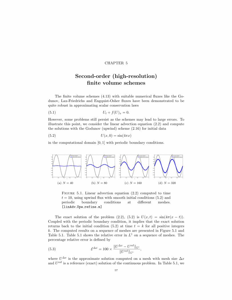
CHAPTER 5
Second-order (high-resolution)finite volume schemes
The finite volume schemes (4.13) with suitable numerical fluxes like the Go-dunov, Lax-Friedrichs and Engquist-Osher fluxes have been demonstrated to bequite robust in approximating scalar conservation laws
(5.1) Ut + f(U)x = 0.
However, some problems still persist as the schemes may lead to large errors. Toillustrate this point, we consider the linear advection equation (2.2) and computethe solutions with the Godunov (upwind) scheme (2.16) for initial data
(5.2) U(x, 0) = sin(4πx)
in the computational domain [0, 1] with periodic boundary conditions.
0 0.2 0.4 0.6 0.8 1−1
−0.8
−0.6
−0.4
−0.2
0
0.2
0.4
0.6
0.8
1
x
Exact solutionApproximate solution
(a) N = 40
0 0.2 0.4 0.6 0.8 1−1
−0.8
−0.6
−0.4
−0.2
0
0.2
0.4
0.6
0.8
1
x
Exact solutionApproximate solution
(b) N = 80
0 0.2 0.4 0.6 0.8 1−1
−0.8
−0.6
−0.4
−0.2
0
0.2
0.4
0.6
0.8
1
x
Exact solutionApproximate solution
(c) N = 160
0 0.2 0.4 0.6 0.8 1−1
−0.8
−0.6
−0.4
−0.2
0
0.2
0.4
0.6
0.8
1
x
Exact solutionApproximate solution
(d) N = 320
Figure 5.1. Linear advection equation (2.2) computed to timet = 10, using upwind flux with smooth initial conditions (5.2) andperiodic boundary conditions at different meshes.[linAdv Upw refine.m]
The exact solution of the problem (2.2), (5.2) is U(x, t) = sin(4π(x − t)).Coupled with the periodic boundary condition, it implies that the exact solutionreturns back to the initial condition (5.2) at time t = k for all positive integersk. The computed results on a sequence of meshes are presented in Figure 5.1 andTable 5.1. Table 5.1 shows the relative error in L1 on a sequence of meshes. Thepercentage relative error is defined by
(5.3) E∆x = 100× ‖U∆x − U ref‖L1
‖U ref‖L1
,
where U∆x is the approximate solution computed on a mesh with mesh size ∆xand U ref is a reference (exact) solution of the continuous problem. In Table 5.1, we
57
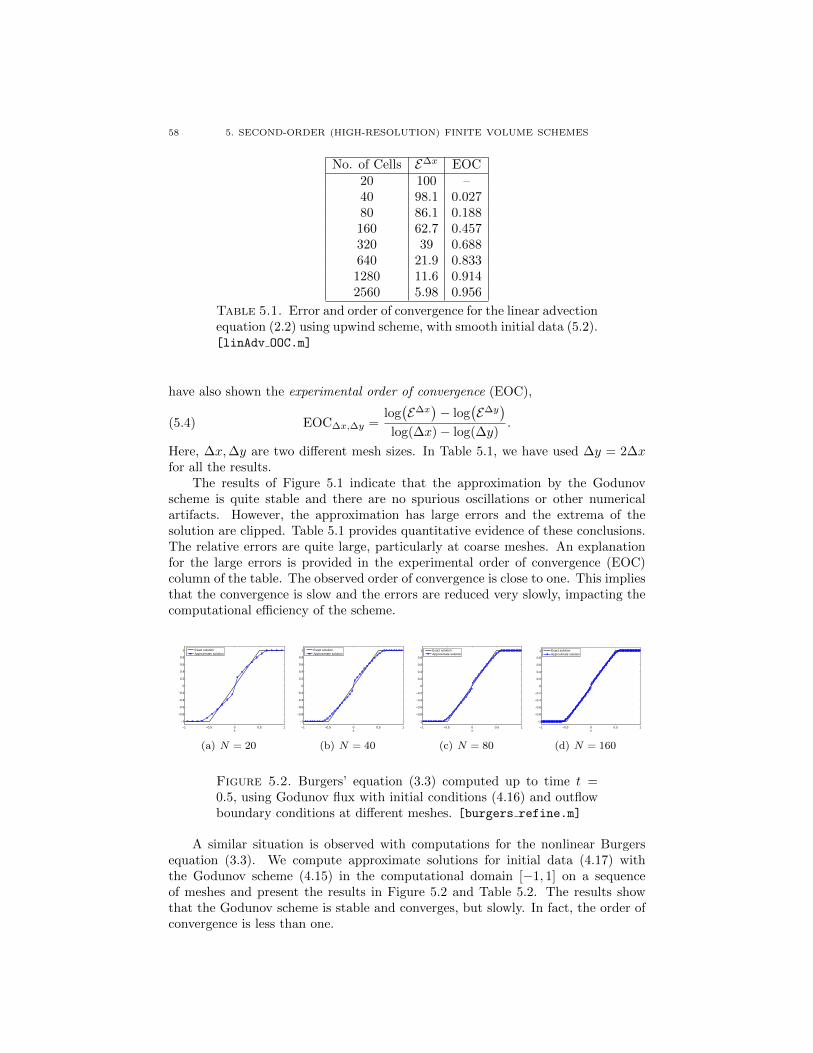
58 5. SECOND-ORDER (HIGH-RESOLUTION) FINITE VOLUME SCHEMES
No. of Cells E∆x EOC20 100 –40 98.1 0.02780 86.1 0.188160 62.7 0.457320 39 0.688640 21.9 0.8331280 11.6 0.9142560 5.98 0.956
Table 5.1. Error and order of convergence for the linear advectionequation (2.2) using upwind scheme, with smooth initial data (5.2).[linAdv OOC.m]
have also shown the experimental order of convergence (EOC),
(5.4) EOC∆x,∆y =log(E∆x
)− log
(E∆y
)log(∆x)− log(∆y)
.
Here, ∆x,∆y are two different mesh sizes. In Table 5.1, we have used ∆y = 2∆xfor all the results.
The results of Figure 5.1 indicate that the approximation by the Godunovscheme is quite stable and there are no spurious oscillations or other numericalartifacts. However, the approximation has large errors and the extrema of thesolution are clipped. Table 5.1 provides quantitative evidence of these conclusions.The relative errors are quite large, particularly at coarse meshes. An explanationfor the large errors is provided in the experimental order of convergence (EOC)column of the table. The observed order of convergence is close to one. This impliesthat the convergence is slow and the errors are reduced very slowly, impacting thecomputational efficiency of the scheme.
−1 −0.5 0 0.5 1
−1
−0.8
−0.6
−0.4
−0.2
0
0.2
0.4
0.6
0.8
1
x
Exact solutionApproximate solution
(a) N = 20
−1 −0.5 0 0.5 1
−1
−0.8
−0.6
−0.4
−0.2
0
0.2
0.4
0.6
0.8
1
x
Exact solutionApproximate solution
(b) N = 40
−1 −0.5 0 0.5 1
−1
−0.8
−0.6
−0.4
−0.2
0
0.2
0.4
0.6
0.8
1
x
Exact solutionApproximate solution
(c) N = 80
−1 −0.5 0 0.5 1
−1
−0.8
−0.6
−0.4
−0.2
0
0.2
0.4
0.6
0.8
1
x
Exact solutionApproximate solution
(d) N = 160
Figure 5.2. Burgers’ equation (3.3) computed up to time t =0.5, using Godunov flux with initial conditions (4.16) and outflowboundary conditions at different meshes. [burgers refine.m]
A similar situation is observed with computations for the nonlinear Burgersequation (3.3). We compute approximate solutions for initial data (4.17) withthe Godunov scheme (4.15) in the computational domain [−1, 1] on a sequenceof meshes and present the results in Figure 5.2 and Table 5.2. The results showthat the Godunov scheme is stable and converges, but slowly. In fact, the order ofconvergence is less than one.
5.1. ORDER OF ACCURACY 59
No. of Cells E∆x EOC20 6.86 –40 4.51 0.60580 2.84 0.667160 1.74 0.706320 1.04 0.745640 0.606 0.7781280 0.347 0.8042560 0.196 0.826
Table 5.2. Error and order of convergence for Burgers’ equation(3.3) using Godunov’s scheme with initial data (4.16).[burgers OOC.m]
Both numerical experiments indicate that the Godunov type finite volumescheme (4.13) is stable but can lead to large errors, due to its slow convergence.A possible recipe for reducing errors is to increase the rate of convergence. Thischapter is devoted to introducing the concepts of truncation errors and order of ac-curacy of schemes. Furthermore, we will construct second-order accurate versionsof the finite volume scheme (4.13) for approximating scalar conservation laws.
5.1. Order of accuracy
The order of accuracy of numerical schemes is a very useful concept in numericalanalysis.
Definition 5.1. Assume that a finite volume scheme for approximating (5.1) canbe written in the generic (2p + 1)-point update form (4.38), and that ∆t
∆x ≡ λ forsome constant λ > 0. The truncation error of the scheme is defined as
(5.5) Tj,n = U(xj , tn+1)−H
(U(xj−p, t
n), . . . , U(xj+p, tn)),
where U is the exact solution. The scheme is q-th order accurate if q ∈ N is thelargest integer for which
(5.6) Tj,n = O(∆tq+1
)for all j, n
as ∆t→ 0.
Lemma 5.2. Assume that the exact solution U(x, t) of the scalar conservation lawis C2, and that a consistent and conservative three-point finite volume method hasa C2 update function H. Then the scheme is at least first-order accurate.
Proof. As the solution and the update function H in (4.45) are at least twicecontinuously differentiable, we can use Taylor expansions. We write the updatefunction as H = H(X,Y, Z). From (4.45) and (4.13) we get
(5.7)
∂H
∂X(Unj−1, U
nj , U
nj+1) =
∆t
∆x
∂F
∂a(Unj−1, U
nj ),
∂H
∂Z(Unj−1, U
nj , U
nj+1) = −∆t
∆x
∂F
∂b(Unj , U
nj+1).
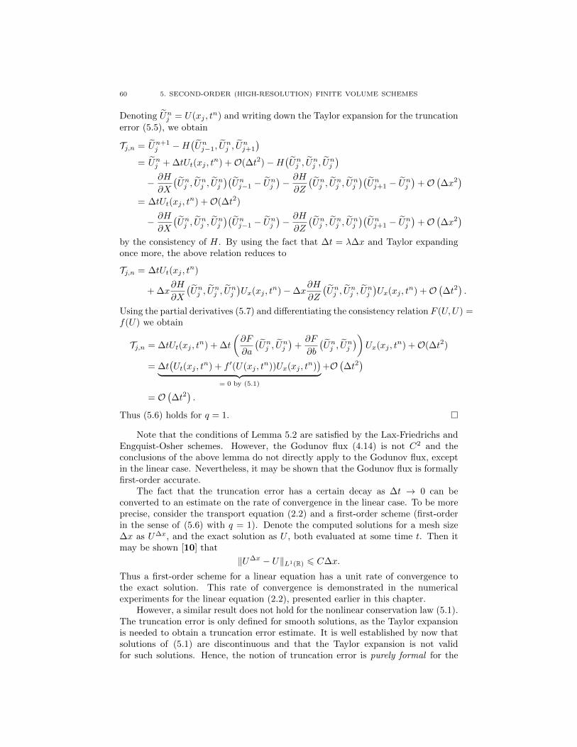
60 5. SECOND-ORDER (HIGH-RESOLUTION) FINITE VOLUME SCHEMES
Denoting Unj = U(xj , tn) and writing down the Taylor expansion for the truncation
error (5.5), we obtain
Tj,n = Un+1j −H
(Unj−1, U
nj , U
nj+1
)= Unj + ∆tUt(xj , t
n) +O(∆t2)−H(Unj , U
nj , U
nj
)− ∂H
∂X
(Unj , U
nj , U
nj
)(Unj−1 − Unj
)− ∂H
∂Z
(Unj , U
nj , U
nj
)(Unj+1 − Unj
)+O
(∆x2
)= ∆tUt(xj , t
n) +O(∆t2)
− ∂H
∂X
(Unj , U
nj , U
nj
)(Unj−1 − Unj
)− ∂H
∂Z
(Unj , U
nj , U
nj
)(Unj+1 − Unj
)+O
(∆x2
)by the consistency of H. By using the fact that ∆t = λ∆x and Taylor expandingonce more, the above relation reduces to
Tj,n = ∆tUt(xj , tn)
+ ∆x∂H
∂X
(Unj , U
nj , U
nj
)Ux(xj , t
n)−∆x∂H
∂Z
(Unj , U
nj , U
nj
)Ux(xj , t
n) +O(∆t2
).
Using the partial derivatives (5.7) and differentiating the consistency relation F (U,U) =f(U) we obtain
Tj,n = ∆tUt(xj , tn) + ∆t
(∂F
∂a
(Unj , U
nj
)+∂F
∂b
(Unj , U
nj
))Ux(xj , t
n) +O(∆t2)
= ∆t(Ut(xj , t
n) + f ′(U(xj , tn))Ux(xj , t
n))︸ ︷︷ ︸
= 0 by (5.1)
+O(∆t2
)= O
(∆t2
).
Thus (5.6) holds for q = 1.
Note that the conditions of Lemma 5.2 are satisfied by the Lax-Friedrichs andEngquist-Osher schemes. However, the Godunov flux (4.14) is not C2 and theconclusions of the above lemma do not directly apply to the Godunov flux, exceptin the linear case. Nevertheless, it may be shown that the Godunov flux is formallyfirst-order accurate.
The fact that the truncation error has a certain decay as ∆t → 0 can beconverted to an estimate on the rate of convergence in the linear case. To be moreprecise, consider the transport equation (2.2) and a first-order scheme (first-orderin the sense of (5.6) with q = 1). Denote the computed solutions for a mesh size∆x as U∆x, and the exact solution as U , both evaluated at some time t. Then itmay be shown [10] that
‖U∆x − U‖L1(R) 6 C∆x.
Thus a first-order scheme for a linear equation has a unit rate of convergence tothe exact solution. This rate of convergence is demonstrated in the numericalexperiments for the linear equation (2.2), presented earlier in this chapter.
However, a similar result does not hold for the nonlinear conservation law (5.1).The truncation error is only defined for smooth solutions, as the Taylor expansionis needed to obtain a truncation error estimate. It is well established by now thatsolutions of (5.1) are discontinuous and that the Taylor expansion is not validfor such solutions. Hence, the notion of truncation error is purely formal for the
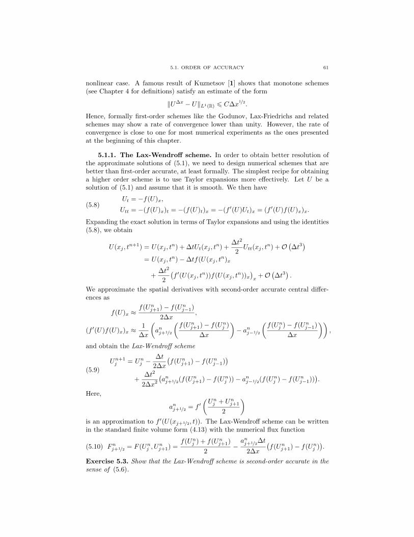
5.1. ORDER OF ACCURACY 61
nonlinear case. A famous result of Kuznetsov [1] shows that monotone schemes(see Chapter 4 for definitions) satisfy an estimate of the form
‖U∆x − U‖L1(R) 6 C∆x1/2.
Hence, formally first-order schemes like the Godunov, Lax-Friedrichs and relatedschemes may show a rate of convergence lower than unity. However, the rate ofconvergence is close to one for most numerical experiments as the ones presentedat the beginning of this chapter.
5.1.1. The Lax-Wendroff scheme. In order to obtain better resolution ofthe approximate solutions of (5.1), we need to design numerical schemes that arebetter than first-order accurate, at least formally. The simplest recipe for obtaininga higher order scheme is to use Taylor expansions more effectively. Let U be asolution of (5.1) and assume that it is smooth. We then have
(5.8)Ut = −f(U)x,
Utt = −(f(U)x)t = −(f(U)t)x = −(f ′(U)Ut)x = (f ′(U)f(U)x)x.
Expanding the exact solution in terms of Taylor expansions and using the identities(5.8), we obtain
U(xj , tn+1) = U(xj , t
n) + ∆tUt(xj , tn) +
∆t2
2Utt(xj , t
n) +O(∆t3
)= U(xj , t
n)−∆tf(U(xj , tn)x
+∆t2
2
(f ′(U(xj , t
n))f(U(xj , tn))x
)x
+O(∆t3
).
We approximate the spatial derivatives with second-order accurate central differ-ences as
f(U)x ≈f(Unj+1)− f(Unj−1)
2∆x,
(f ′(U)f(U)x)x ≈1
∆x
(anj+1/2
(f(Unj+1)− f(Unj )
∆x
)− anj−1/2
(f(Unj )− f(Unj−1)
∆x
)),
and obtain the Lax-Wendroff scheme
(5.9)
Un+1j = Unj −
∆t
2∆x
(f(Unj+1)− f(Unj−1)
)+
∆t2
2∆x2
(anj+1/2(f(Unj+1)− f(Unj ))− anj−1/2(f(Unj )− f(Unj−1))
).
Here,
anj+1/2 = f ′(Unj + Unj+1
2
)is an approximation to f ′(U(xj+1/2, t)). The Lax-Wendroff scheme can be writtenin the standard finite volume form (4.13) with the numerical flux function
(5.10) Fnj+1/2 = F (Unj , Unj+1) =
f(Unj ) + f(Unj+1)
2−anj+1/2∆t
2∆x
(f(Unj+1)− f(Unj )
).
Exercise 5.3. Show that the Lax-Wendroff scheme is second-order accurate in thesense of (5.6).
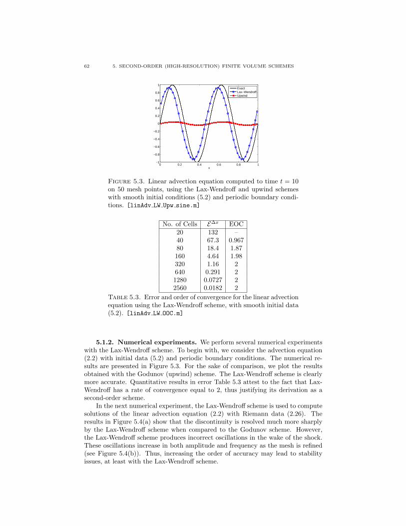
62 5. SECOND-ORDER (HIGH-RESOLUTION) FINITE VOLUME SCHEMES
0 0.2 0.4 0.6 0.8 1−1
−0.8
−0.6
−0.4
−0.2
0
0.2
0.4
0.6
0.8
1
x
ExactLax−WendroffUpwind
Figure 5.3. Linear advection equation computed to time t = 10on 50 mesh points, using the Lax-Wendroff and upwind schemeswith smooth initial conditions (5.2) and periodic boundary condi-tions. [linAdv LW Upw sine.m]
No. of Cells E∆x EOC20 132 –40 67.3 0.96780 18.4 1.87160 4.64 1.98320 1.16 2640 0.291 21280 0.0727 22560 0.0182 2
Table 5.3. Error and order of convergence for the linear advectionequation using the Lax-Wendroff scheme, with smooth initial data(5.2). [linAdv LW OOC.m]
5.1.2. Numerical experiments. We perform several numerical experimentswith the Lax-Wendroff scheme. To begin with, we consider the advection equation(2.2) with initial data (5.2) and periodic boundary conditions. The numerical re-sults are presented in Figure 5.3. For the sake of comparison, we plot the resultsobtained with the Godunov (upwind) scheme. The Lax-Wendroff scheme is clearlymore accurate. Quantitative results in error Table 5.3 attest to the fact that Lax-Wendroff has a rate of convergence equal to 2, thus justifying its derivation as asecond-order scheme.
In the next numerical experiment, the Lax-Wendroff scheme is used to computesolutions of the linear advection equation (2.2) with Riemann data (2.26). Theresults in Figure 5.4(a) show that the discontinuity is resolved much more sharplyby the Lax-Wendroff scheme when compared to the Godunov scheme. However,the Lax-Wendroff scheme produces incorrect oscillations in the wake of the shock.These oscillations increase in both amplitude and frequency as the mesh is refined(see Figure 5.4(b)). Thus, increasing the order of accuracy may lead to stabilityissues, at least with the Lax-Wendroff scheme.

5.2. THE REA ALGORITHM 63
0 0.5 1 1.5 21
1.2
1.4
1.6
1.8
2
x
ExactLax−WendroffUpwind
(a) 100 grid points
0 0.5 1 1.5 21
1.2
1.4
1.6
1.8
2
2.2
x
ExactLax−WendroffUpwind
(b) 1000 grid points
Figure 5.4. Linear advection equation computed to time t = 1with discontinuous initial conditions (2.26) and outflow boundaryconditions. Comparison of the Lax-Wendroff and upwind schemes.[linAdv LW Upw disc.m]
−1 −0.5 0 0.5 10
0.2
0.4
0.6
0.8
1
x
ExactLax−WendroffGodunov
Figure 5.5. Burgers’ equation computed to time t = 0.5 withdiscontinuous initial conditions (4.16) and outflow boundary con-ditions on 50 cells. [burgers LW God disc.m]
As another numerical example, consider the nonlinear Burgers equation (3.3)with Riemann data (4.16). The results, shown in Figure 5.5, show that although theLax-Wendroff scheme resolves the shock slightly better than the Godunov scheme,the solution is polluted with spurious oscillations. In conclusion, the Lax-Wendroffscheme fails to resolve discontinuous solutions of conservation laws in a stable,monotonous manner.
5.2. The REA algorithm
Given the instabilities that result from the Lax-Wendroff scheme, we need todevise a new procedure for obtaining high-order schemes. This forces us to revisitthe original derivation of the Godunov scheme, presented in Chapter 4. It turns
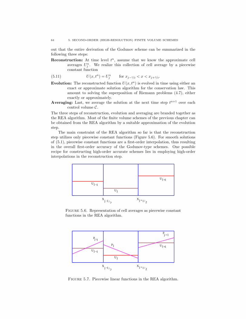
64 5. SECOND-ORDER (HIGH-RESOLUTION) FINITE VOLUME SCHEMES
out that the entire derivation of the Godunov scheme can be summarized in thefollowing three steps:
Reconstruction: At time level tn, assume that we know the approximate cellaverages Unj . We realize this collection of cell average by a piecewiseconstant function
(5.11) U(x, tn) = Unj for xj−1/2 < x < xj+1/2.
Evolution: The reconstructed function U(x, tn) is evolved in time using either anexact or approximate solution algorithm for the conservation law. Thisamount to solving the superposition of Riemann problems (4.7), eitherexactly or approximately.
Averaging: Last, we average the solution at the next time step tn+1 over eachcontrol volume C.
The three steps of reconstruction, evolution and averaging are branded together asthe REA algorithm. Most of the finite volume schemes of the previous chapter canbe obtained from the REA algorithm by a suitable approximation of the evolutionstep.
The main constraint of the REA algorithm so far is that the reconstructionstep utilizes only piecewise constant functions (Figure 5.6). For smooth solutionsof (5.1), piecewise constant functions are a first-order interpolation, thus resultingin the overall first-order accuracy of the Godunov-type schemes. One possiblerecipe for constructing high-order accurate schemes lies in employing high-orderinterpolations in the reconstruction step.
X−j 1/ 2
X j +1 /2
Uj −1
Uj
Uj +1
Figure 5.6. Representation of cell averages as piecewise constantfunctions in the REA algorithm.
X−j 1/ 2
X j +1 /2
Uj −1
Uj
Uj +1
j p
−1
pj
j p
+1
Figure 5.7. Piecewise linear functions in the REA algorithm.
5.2. THE REA ALGORITHM 65
5.2.1. Second-order reconstruction. The simplest high-order interpolationresults from a piecewise linear reconstruction (Figure 5.7). Such a reconstructionwill lead to a second-order accurate rendition of the smooth solutions of (5.1).Given the cell averages Unj at time tn, there are several possibilities for recon-structing linear functions in each cell Cj . We need to narrow down the alternativesby putting constraints on the reconstruction.
One of the key requirements for a stable and convergent approximation ofconservation laws is that the scheme is conservative (4.39).
Exercise 5.4. Show that the evolution and averaging steps are conservative byverifying that
(a) if U(x, tn+1) is the exact solution at time tn+1, then∫RU(x, tn+1) dx =
∫RU(x, tn) dx,
(b) if Un+1j is the average of U(x, tn+1) in cell j, then
∆x∑j
Un+1j =
∫RU(x, tn+1) dx.
It is natural to demand that the reconstruction step is also conservative. De-noting the piecewise linear function in the cell Cj as pj(x), we require that
(5.12)1
∆x
∫ xj+1/2
xj−1/2
pj(x)dx = Unj .
It is readily seen that pj must have the form
(5.13) pj(x) = Unj + σnj (x− xj),
where σnj is a parameter that determines the slope in cell Cj . The local linearfunctions pj are combined to define the global piecewise linear function
(5.14) p(x) = pj(x) for xj−1/2 < x < xj+1/2.
This piecewise linear function can be used with the REA algorithm to obtain ahigher order scheme.
5.2.2. Choices of slope. The slope σ in (5.13) can be determined in a varietyof ways. Three of them are
• Central:
(5.15) σnj =Unj+1 − Unj−1
2∆x.
• Backward:
(5.16) σnj =Unj − Unj−1
∆x.
• Forward:
(5.17) σnj =Unj+1 − Unj
∆x.
It is instructive to see what scheme the REA algorithm with the above choices ofslope results in. For simplicity of the exposition, we consider the linear advectionequation (2.2) with a positive velocity a > 0.
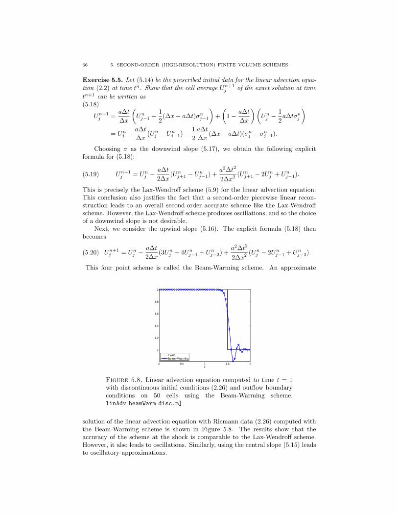
66 5. SECOND-ORDER (HIGH-RESOLUTION) FINITE VOLUME SCHEMES
Exercise 5.5. Let (5.14) be the prescribed initial data for the linear advection equa-tion (2.2) at time tn. Show that the cell average Un+1
j of the exact solution at time
tn+1 can be written as(5.18)
Un+1j =
a∆t
∆x
(Unj−1 +
1
2(∆x− a∆t)σnj−1
)+
(1− a∆t
∆x
)(Unj −
1
2a∆tσnj
)= Unj −
a∆t
∆x
(Unj − Unj−1
)− 1
2
a∆t
∆x(∆x− a∆t)(σnj − σnj−1).
Choosing σ as the downwind slope (5.17), we obtain the following explicitformula for (5.18):
(5.19) Un+1j = Unj −
a∆t
2∆x(Unj+1 − Unj−1) +
a2∆t2
2∆x2 (Unj+1 − 2Unj + Unj−1).
This is precisely the Lax-Wendroff scheme (5.9) for the linear advection equation.This conclusion also justifies the fact that a second-order piecewise linear recon-struction leads to an overall second-order accurate scheme like the Lax-Wendroffscheme. However, the Lax-Wendroff scheme produces oscillations, and so the choiceof a downwind slope is not desirable.
Next, we consider the upwind slope (5.16). The explicit formula (5.18) thenbecomes
(5.20) Un+1j = Unj −
a∆t
2∆x(3Unj − 4Unj−1 + Unj−2) +
a2∆t2
2∆x2 (Unj − 2Unj−1 + Unj−2).
This four point scheme is called the Beam-Warming scheme. An approximate
0 0.5 1 1.5 2
1
1.2
1.4
1.6
1.8
2
x
ExactBeam−Warming
Figure 5.8. Linear advection equation computed to time t = 1with discontinuous initial conditions (2.26) and outflow boundaryconditions on 50 cells using the Beam-Warming scheme.linAdv beamWarm disc.m]
solution of the linear advection equation with Riemann data (2.26) computed withthe Beam-Warming scheme is shown in Figure 5.8. The results show that theaccuracy of the scheme at the shock is comparable to the Lax-Wendroff scheme.However, it also leads to oscillations. Similarly, using the central slope (5.15) leadsto oscillatory approximations.
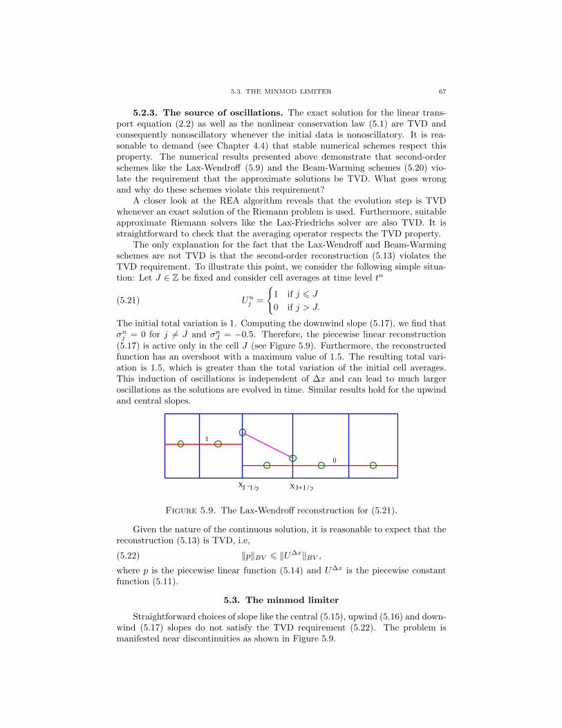
5.3. THE MINMOD LIMITER 67
5.2.3. The source of oscillations. The exact solution for the linear trans-port equation (2.2) as well as the nonlinear conservation law (5.1) are TVD andconsequently nonoscillatory whenever the initial data is nonoscillatory. It is rea-sonable to demand (see Chapter 4.4) that stable numerical schemes respect thisproperty. The numerical results presented above demonstrate that second-orderschemes like the Lax-Wendroff (5.9) and the Beam-Warming schemes (5.20) vio-late the requirement that the approximate solutions be TVD. What goes wrongand why do these schemes violate this requirement?
A closer look at the REA algorithm reveals that the evolution step is TVDwhenever an exact solution of the Riemann problem is used. Furthermore, suitableapproximate Riemann solvers like the Lax-Friedrichs solver are also TVD. It isstraightforward to check that the averaging operator respects the TVD property.
The only explanation for the fact that the Lax-Wendroff and Beam-Warmingschemes are not TVD is that the second-order reconstruction (5.13) violates theTVD requirement. To illustrate this point, we consider the following simple situa-tion: Let J ∈ Z be fixed and consider cell averages at time level tn
(5.21) Unj =
1 if j 6 J
0 if j > J.
The initial total variation is 1. Computing the downwind slope (5.17), we find thatσnj = 0 for j 6= J and σnJ = −0.5. Therefore, the piecewise linear reconstruction(5.17) is active only in the cell J (see Figure 5.9). Furthermore, the reconstructedfunction has an overshoot with a maximum value of 1.5. The resulting total vari-ation is 1.5, which is greater than the total variation of the initial cell averages.This induction of oscillations is independent of ∆x and can lead to much largeroscillations as the solutions are evolved in time. Similar results hold for the upwindand central slopes.
XJ−1/2 X J+1/2
0
1
Figure 5.9. The Lax-Wendroff reconstruction for (5.21).
Given the nature of the continuous solution, it is reasonable to expect that thereconstruction (5.13) is TVD, i.e,
(5.22) ‖p‖BV 6 ‖U∆x‖BV ,where p is the piecewise linear function (5.14) and U∆x is the piecewise constantfunction (5.11).
5.3. The minmod limiter
Straightforward choices of slope like the central (5.15), upwind (5.16) and down-wind (5.17) slopes do not satisfy the TVD requirement (5.22). The problem ismanifested near discontinuities as shown in Figure 5.9.
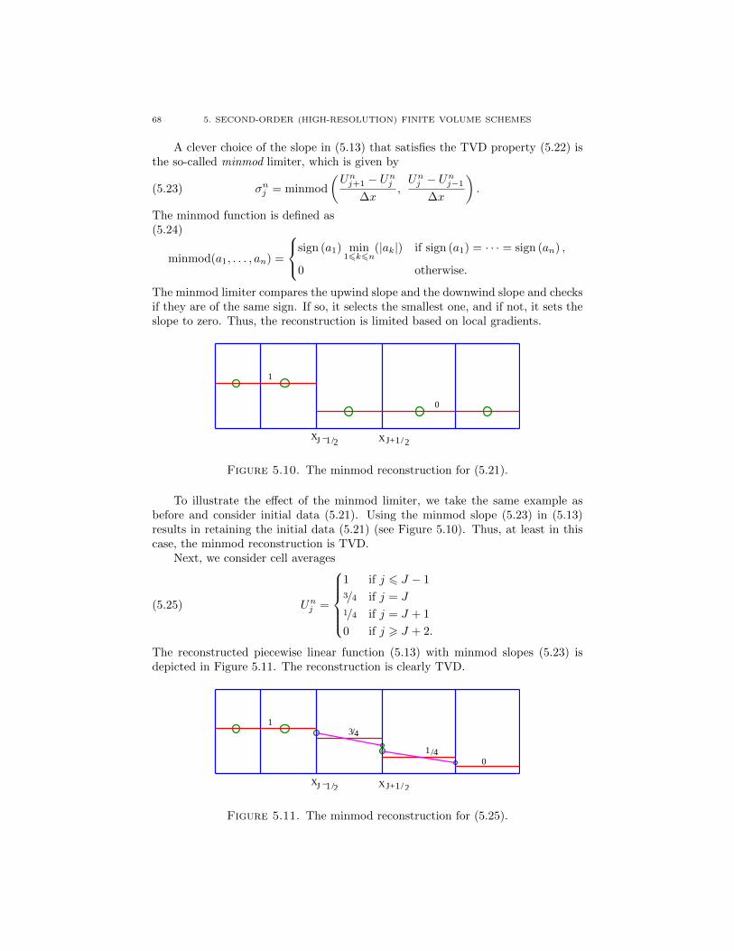
68 5. SECOND-ORDER (HIGH-RESOLUTION) FINITE VOLUME SCHEMES
A clever choice of the slope in (5.13) that satisfies the TVD property (5.22) isthe so-called minmod limiter, which is given by
(5.23) σnj = minmod
(Unj+1 − Unj
∆x,Unj − Unj−1
∆x
).
The minmod function is defined as(5.24)
minmod(a1, . . . , an) =
sign (a1) min16k6n
(|ak|) if sign (a1) = · · · = sign (an) ,
0 otherwise.
The minmod limiter compares the upwind slope and the downwind slope and checksif they are of the same sign. If so, it selects the smallest one, and if not, it sets theslope to zero. Thus, the reconstruction is limited based on local gradients.
XJ−1/2 X J+1/2
0
1
Figure 5.10. The minmod reconstruction for (5.21).
To illustrate the effect of the minmod limiter, we take the same example asbefore and consider initial data (5.21). Using the minmod slope (5.23) in (5.13)results in retaining the initial data (5.21) (see Figure 5.10). Thus, at least in thiscase, the minmod reconstruction is TVD.
Next, we consider cell averages
(5.25) Unj =
1 if j 6 J − 13/4 if j = J1/4 if j = J + 1
0 if j > J + 2.
The reconstructed piecewise linear function (5.13) with minmod slopes (5.23) isdepicted in Figure 5.11. The reconstruction is clearly TVD.
XJ−1/2 X J+1/2
13/4
1/40
Figure 5.11. The minmod reconstruction for (5.25).
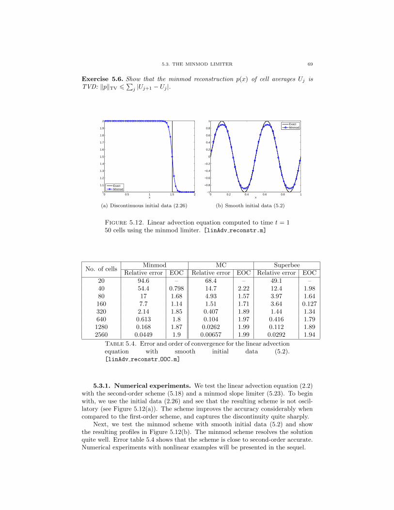
5.3. THE MINMOD LIMITER 69
Exercise 5.6. Show that the minmod reconstruction p(x) of cell averages Uj isTVD: ‖p‖TV 6
∑j |Uj+1 − Uj |.
0 0.5 1 1.5 21
1.1
1.2
1.3
1.4
1.5
1.6
1.7
1.8
1.9
2
x
ExactMinmod
(a) Discontinuous initial data (2.26)
0 0.2 0.4 0.6 0.8 1−1
−0.8
−0.6
−0.4
−0.2
0
0.2
0.4
0.6
0.8
1
x
ExactMinmod
(b) Smooth initial data (5.2)
Figure 5.12. Linear advection equation computed to time t = 150 cells using the minmod limiter. [linAdv reconstr.m]
No. of cellsMinmod MC Superbee
Relative error EOC Relative error EOC Relative error EOC20 94.6 – 68.4 – 49.1 –40 54.4 0.798 14.7 2.22 12.4 1.9880 17 1.68 4.93 1.57 3.97 1.64160 7.7 1.14 1.51 1.71 3.64 0.127320 2.14 1.85 0.407 1.89 1.44 1.34640 0.613 1.8 0.104 1.97 0.416 1.791280 0.168 1.87 0.0262 1.99 0.112 1.892560 0.0449 1.9 0.00657 1.99 0.0292 1.94
Table 5.4. Error and order of convergence for the linear advectionequation with smooth initial data (5.2).[linAdv reconstr OOC.m]
5.3.1. Numerical experiments. We test the linear advection equation (2.2)with the second-order scheme (5.18) and a minmod slope limiter (5.23). To beginwith, we use the initial data (2.26) and see that the resulting scheme is not oscil-latory (see Figure 5.12(a)). The scheme improves the accuracy considerably whencompared to the first-order scheme, and captures the discontinuity quite sharply.
Next, we test the minmod scheme with smooth initial data (5.2) and showthe resulting profiles in Figure 5.12(b). The minmod scheme resolves the solutionquite well. Error table 5.4 shows that the scheme is close to second-order accurate.Numerical experiments with nonlinear examples will be presented in the sequel.
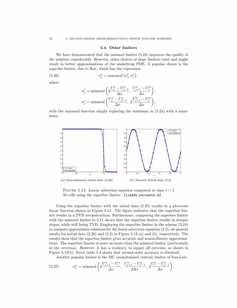
70 5. SECOND-ORDER (HIGH-RESOLUTION) FINITE VOLUME SCHEMES
5.4. Other limiters
We have demonstrated that the minmod limiter (5.23) improves the quality ofthe solution considerably. However, other choices of slope limiters exist and mightresult in better approximations of the underlying PDE. A popular choice is thesuperbee limiter, due to Roe, which has the expression
(5.26) σnj = maxmod(σlj , σ
rj
),
where
σlj = minmod
(2Unj − Unj−1
∆x,Unj+1 − Unj
∆x
),
σrj = minmod
(Unj − Unj−1
∆x, 2
Unj+1 − Unj∆x
),
with the maxmod function simply replacing the minimum in (5.24) with a maxi-mum.
0 0.5 1 1.5 21
1.1
1.2
1.3
1.4
1.5
1.6
1.7
1.8
1.9
2
x
ExactSuperbee
(a) Discontinuous initial data (2.26)
0 0.2 0.4 0.6 0.8 1−1
−0.8
−0.6
−0.4
−0.2
0
0.2
0.4
0.6
0.8
1
x
ExactSuperbee
(b) Smooth initial data (5.2)
Figure 5.13. Linear advection equation computed to time t = 150 cells using the superbee limiter. [linAdv reconstr.m]
Using the superbee limiter with the initial data (5.25) results in a piecewiselinear function shown in Figure 5.14. The figure indicates that the superbee lim-iter results in a TVD reconstruction. Furthermore, comparing the superbee limiterwith the minmod limiter in 5.11 shows that the superbee limiter results in steeperslopes, while still being TVD. Employing the superbee limiter in the scheme (5.18)to compute approximate solutions for the linear advection equation (2.2), we presentresults for initial data (2.26) and (5.2) in Figure 5.13 (a) and (b), respectively. Theresults show that the superbee limiter gives accurate and nonoscillatory approxima-tions. The superbee limiter is more accurate than the minmod limiter (particularlyat the extrema). However, it has a tendency to square off extrema, as shown inFigure 5.13(b). Error table 5.4 shows that second-order accuracy is obtained.
Another popular limiter is the MC (monotonized central) limiter of Van-Leer,
(5.27) σnj = minmod
(2Unj+1 − Unj
∆x,Unj+1 − Unj−1
2∆x, 2
Unj − Unj−1
∆x
).
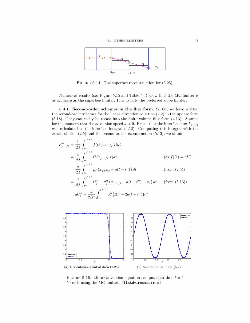
5.4. OTHER LIMITERS 71
XJ−1/2 X J+1/2
13/4
1/40
Figure 5.14. The superbee reconstruction for (5.25).
Numerical results (see Figure 5.15 and Table 5.4) show that the MC limiter isas accurate as the superbee limiter. It is usually the preferred slope limiter.
5.4.1. Second-order schemes in the flux form. So far, we have writtenthe second-order schemes for the linear advection equation (2.2) in the update form(5.18). They can easily be recast into the finite volume flux form (4.13). Assumefor the moment that the advection speed a > 0. Recall that the interface flux Fi+1/2
was calculated as the interface integral (4.12). Computing this integral with theexact solution (2.5) and the second-order reconstruction (5.13), we obtain
Fnj+1/2 =1
∆t
∫ tn+1
tnf(U(xj+1/2, t)dt
=a
∆t
∫ tn+1
tnU(xj+1/2, t)dt (as f(U) = aU)
=a
∆t
∫ tn+1
tnpj(xj+1/2 − a(t− tn)
)dt (from (2.5))
=a
∆t
∫ tn+1
tnUnj + σnj
(xj+1/2 − a(t− tn)− xj
)dt (from (5.13))
= aUnj +a
2∆t
∫ tn+1
tnσnj(∆x− 2a(t− tn)
)dt
0 0.5 1 1.5 21
1.1
1.2
1.3
1.4
1.5
1.6
1.7
1.8
1.9
2
x
ExactMC
(a) Discontinuous initial data (2.26)
0 0.2 0.4 0.6 0.8 1−1
−0.8
−0.6
−0.4
−0.2
0
0.2
0.4
0.6
0.8
1
x
ExactMC
(b) Smooth initial data (5.2)
Figure 5.15. Linear advection equation computed to time t = 150 cells using the MC limiter. [linAdv reconstr.m]
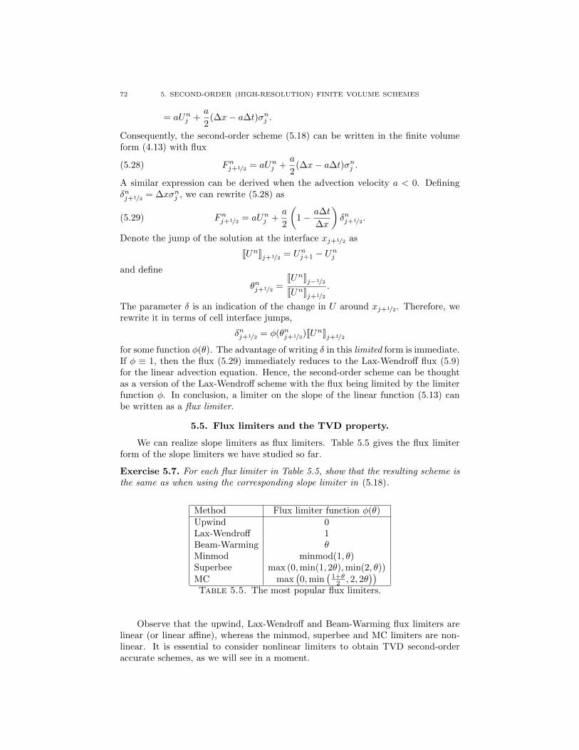
72 5. SECOND-ORDER (HIGH-RESOLUTION) FINITE VOLUME SCHEMES
= aUnj +a
2(∆x− a∆t)σnj .
Consequently, the second-order scheme (5.18) can be written in the finite volumeform (4.13) with flux
(5.28) Fnj+1/2 = aUnj +a
2(∆x− a∆t)σnj .
A similar expression can be derived when the advection velocity a < 0. Definingδnj+1/2 = ∆xσnj , we can rewrite (5.28) as
(5.29) Fnj+1/2 = aUnj +a
2
(1− a∆t
∆x
)δnj+1/2.
Denote the jump of the solution at the interface xj+1/2 as
[[Un]]j+1/2 = Unj+1 − Unjand define
θnj+1/2 =[[Un]]j−1/2
[[Un]]j+1/2
.
The parameter δ is an indication of the change in U around xj+1/2. Therefore, werewrite it in terms of cell interface jumps,
δnj+1/2 = φ(θnj+1/2)[[Un]]j+1/2
for some function φ(θ). The advantage of writing δ in this limited form is immediate.If φ ≡ 1, then the flux (5.29) immediately reduces to the Lax-Wendroff flux (5.9)for the linear advection equation. Hence, the second-order scheme can be thoughtas a version of the Lax-Wendroff scheme with the flux being limited by the limiterfunction φ. In conclusion, a limiter on the slope of the linear function (5.13) canbe written as a flux limiter.
5.5. Flux limiters and the TVD property.
We can realize slope limiters as flux limiters. Table 5.5 gives the flux limiterform of the slope limiters we have studied so far.
Exercise 5.7. For each flux limiter in Table 5.5, show that the resulting scheme isthe same as when using the corresponding slope limiter in (5.18).
Method Flux limiter function φ(θ)Upwind 0Lax-Wendroff 1Beam-Warming θMinmod minmod(1, θ)Superbee max (0,min(1, 2θ),min(2, θ))MC max
(0,min
(1+θ
2 , 2, 2θ))
Table 5.5. The most popular flux limiters.
Observe that the upwind, Lax-Wendroff and Beam-Warming flux limiters arelinear (or linear affine), whereas the minmod, superbee and MC limiters are non-linear. It is essential to consider nonlinear limiters to obtain TVD second-orderaccurate schemes, as we will see in a moment.
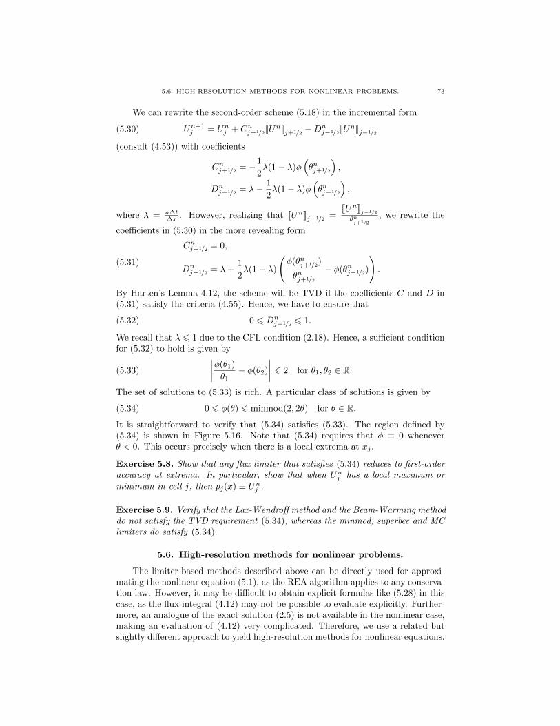
5.6. HIGH-RESOLUTION METHODS FOR NONLINEAR PROBLEMS. 73
We can rewrite the second-order scheme (5.18) in the incremental form
(5.30) Un+1j = Unj + Cnj+1/2[[U
n]]j+1/2 −Dnj−1/2[[U
n]]j−1/2
(consult (4.53)) with coefficients
Cnj+1/2 = −1
2λ(1− λ)φ
(θnj+1/2
),
Dnj−1/2 = λ− 1
2λ(1− λ)φ
(θnj−1/2
),
where λ = a∆t∆x . However, realizing that [[Un]]j+1/2 =
[[Un]]j−1/2
θnj+1/2
, we rewrite the
coefficients in (5.30) in the more revealing form
(5.31)
Cnj+1/2 = 0,
Dnj−1/2 = λ+
1
2λ(1− λ)
(φ(θnj+1/2)
θnj+1/2
− φ(θnj−1/2)
).
By Harten’s Lemma 4.12, the scheme will be TVD if the coefficients C and D in(5.31) satisfy the criteria (4.55). Hence, we have to ensure that
(5.32) 0 6 Dnj−1/2 6 1.
We recall that λ 6 1 due to the CFL condition (2.18). Hence, a sufficient conditionfor (5.32) to hold is given by
(5.33)
∣∣∣∣φ(θ1)
θ1− φ(θ2)
∣∣∣∣ 6 2 for θ1, θ2 ∈ R.
The set of solutions to (5.33) is rich. A particular class of solutions is given by
(5.34) 0 6 φ(θ) 6 minmod(2, 2θ) for θ ∈ R.
It is straightforward to verify that (5.34) satisfies (5.33). The region defined by(5.34) is shown in Figure 5.16. Note that (5.34) requires that φ ≡ 0 wheneverθ < 0. This occurs precisely when there is a local extrema at xj .
Exercise 5.8. Show that any flux limiter that satisfies (5.34) reduces to first-orderaccuracy at extrema. In particular, show that when Unj has a local maximum orminimum in cell j, then pj(x) ≡ Unj .
Exercise 5.9. Verify that the Lax-Wendroff method and the Beam-Warming methoddo not satisfy the TVD requirement (5.34), whereas the minmod, superbee and MClimiters do satisfy (5.34).
5.6. High-resolution methods for nonlinear problems.
The limiter-based methods described above can be directly used for approxi-mating the nonlinear equation (5.1), as the REA algorithm applies to any conserva-tion law. However, it may be difficult to obtain explicit formulas like (5.28) in thiscase, as the flux integral (4.12) may not be possible to evaluate explicitly. Further-more, an analogue of the exact solution (2.5) is not available in the nonlinear case,making an evaluation of (4.12) very complicated. Therefore, we use a related butslightly different approach to yield high-resolution methods for nonlinear equations.
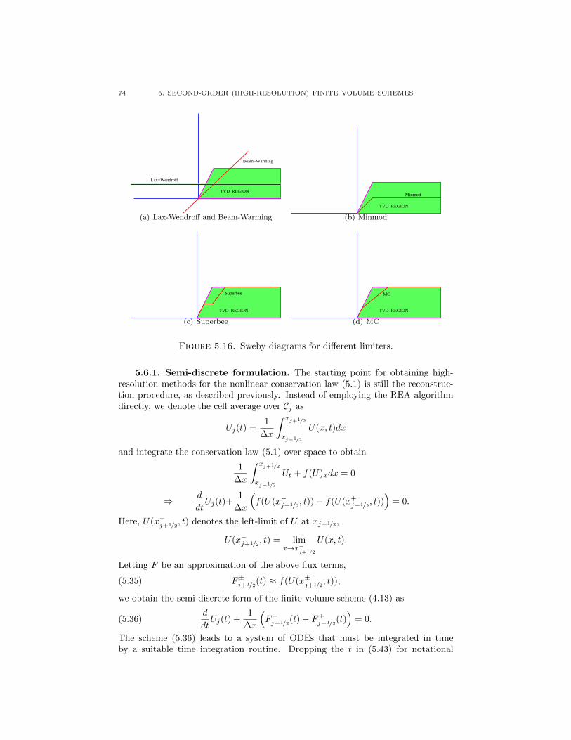
74 5. SECOND-ORDER (HIGH-RESOLUTION) FINITE VOLUME SCHEMES
TVD REGION
Lax−Wendroff
Beam−Warming
(a) Lax-Wendroff and Beam-Warming
TVD REGION
Minmod
(b) Minmod
TVD REGION
Superbee
(c) Superbee
TVD REGION
MC
(d) MC
Figure 5.16. Sweby diagrams for different limiters.
5.6.1. Semi-discrete formulation. The starting point for obtaining high-resolution methods for the nonlinear conservation law (5.1) is still the reconstruc-tion procedure, as described previously. Instead of employing the REA algorithmdirectly, we denote the cell average over Cj as
Uj(t) =1
∆x
∫ xj+1/2
xj−1/2
U(x, t)dx
and integrate the conservation law (5.1) over space to obtain
1
∆x
∫ xj+1/2
xj−1/2
Ut + f(U)xdx = 0
⇒ d
dtUj(t)+
1
∆x
(f(U(x−j+1/2, t))− f(U(x+
j−1/2, t)))
= 0.
Here, U(x−j+1/2, t) denotes the left-limit of U at xj+1/2,
U(x−j+1/2, t) = limx→x−
j+1/2
U(x, t).
Letting F be an approximation of the above flux terms,
(5.35) F±j+1/2(t) ≈ f(U(x±j+1/2, t)),
we obtain the semi-discrete form of the finite volume scheme (4.13) as
(5.36)d
dtUj(t) +
1
∆x
(F−j+1/2(t)− F
+j−1/2(t)
)= 0.
The scheme (5.36) leads to a system of ODEs that must be integrated in timeby a suitable time integration routine. Dropping the t in (5.43) for notational
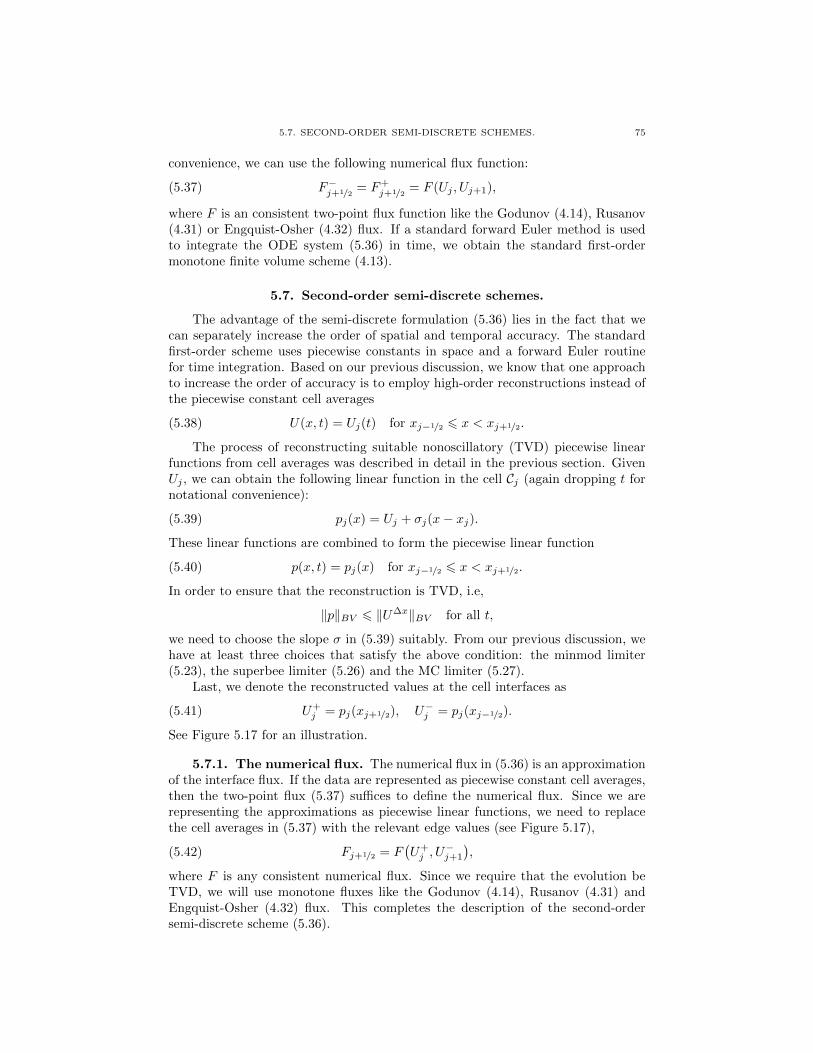
5.7. SECOND-ORDER SEMI-DISCRETE SCHEMES. 75
convenience, we can use the following numerical flux function:
(5.37) F−j+1/2 = F+j+1/2 = F (Uj , Uj+1),
where F is an consistent two-point flux function like the Godunov (4.14), Rusanov(4.31) or Engquist-Osher (4.32) flux. If a standard forward Euler method is usedto integrate the ODE system (5.36) in time, we obtain the standard first-ordermonotone finite volume scheme (4.13).
5.7. Second-order semi-discrete schemes.
The advantage of the semi-discrete formulation (5.36) lies in the fact that wecan separately increase the order of spatial and temporal accuracy. The standardfirst-order scheme uses piecewise constants in space and a forward Euler routinefor time integration. Based on our previous discussion, we know that one approachto increase the order of accuracy is to employ high-order reconstructions instead ofthe piecewise constant cell averages
(5.38) U(x, t) = Uj(t) for xj−1/2 6 x < xj+1/2.
The process of reconstructing suitable nonoscillatory (TVD) piecewise linearfunctions from cell averages was described in detail in the previous section. GivenUj , we can obtain the following linear function in the cell Cj (again dropping t fornotational convenience):
(5.39) pj(x) = Uj + σj(x− xj).
These linear functions are combined to form the piecewise linear function
(5.40) p(x, t) = pj(x) for xj−1/2 6 x < xj+1/2.
In order to ensure that the reconstruction is TVD, i.e,
‖p‖BV 6 ‖U∆x‖BV for all t,
we need to choose the slope σ in (5.39) suitably. From our previous discussion, wehave at least three choices that satisfy the above condition: the minmod limiter(5.23), the superbee limiter (5.26) and the MC limiter (5.27).
Last, we denote the reconstructed values at the cell interfaces as
(5.41) U+j = pj(xj+1/2), U−j = pj(xj−1/2).
See Figure 5.17 for an illustration.
5.7.1. The numerical flux. The numerical flux in (5.36) is an approximationof the interface flux. If the data are represented as piecewise constant cell averages,then the two-point flux (5.37) suffices to define the numerical flux. Since we arerepresenting the approximations as piecewise linear functions, we need to replacethe cell averages in (5.37) with the relevant edge values (see Figure 5.17),
(5.42) Fj+1/2 = F(U+j , U
−j+1
),
where F is any consistent numerical flux. Since we require that the evolution beTVD, we will use monotone fluxes like the Godunov (4.14), Rusanov (4.31) andEngquist-Osher (4.32) flux. This completes the description of the second-ordersemi-discrete scheme (5.36).
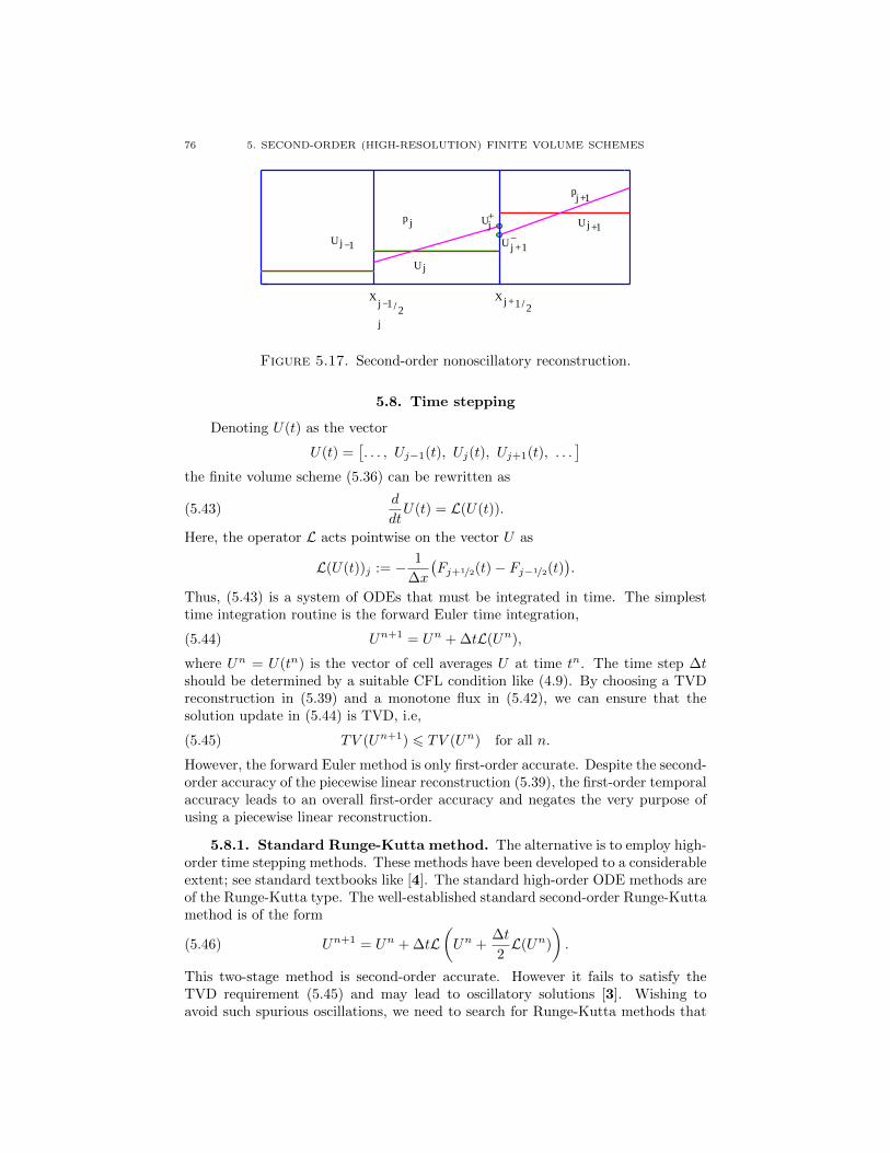
76 5. SECOND-ORDER (HIGH-RESOLUTION) FINITE VOLUME SCHEMES
X−j 1/ 2
X j +1 /2
Uj −1
Uj
Uj +1pj Uj
+
Uj +1
j
−
pj +1
Figure 5.17. Second-order nonoscillatory reconstruction.
5.8. Time stepping
Denoting U(t) as the vector
U(t) =[. . . , Uj−1(t), Uj(t), Uj+1(t), . . .
]the finite volume scheme (5.36) can be rewritten as
(5.43)d
dtU(t) = L(U(t)).
Here, the operator L acts pointwise on the vector U as
L(U(t))j := − 1
∆x
(Fj+1/2(t)− Fj−1/2(t)
).
Thus, (5.43) is a system of ODEs that must be integrated in time. The simplesttime integration routine is the forward Euler time integration,
(5.44) Un+1 = Un + ∆tL(Un),
where Un = U(tn) is the vector of cell averages U at time tn. The time step ∆tshould be determined by a suitable CFL condition like (4.9). By choosing a TVDreconstruction in (5.39) and a monotone flux in (5.42), we can ensure that thesolution update in (5.44) is TVD, i.e,
(5.45) TV (Un+1) 6 TV (Un) for all n.
However, the forward Euler method is only first-order accurate. Despite the second-order accuracy of the piecewise linear reconstruction (5.39), the first-order temporalaccuracy leads to an overall first-order accuracy and negates the very purpose ofusing a piecewise linear reconstruction.
5.8.1. Standard Runge-Kutta method. The alternative is to employ high-order time stepping methods. These methods have been developed to a considerableextent; see standard textbooks like [4]. The standard high-order ODE methods areof the Runge-Kutta type. The well-established standard second-order Runge-Kuttamethod is of the form
(5.46) Un+1 = Un + ∆tL(Un +
∆t
2L(Un)
).
This two-stage method is second-order accurate. However it fails to satisfy theTVD requirement (5.45) and may lead to oscillatory solutions [3]. Wishing toavoid such spurious oscillations, we need to search for Runge-Kutta methods that
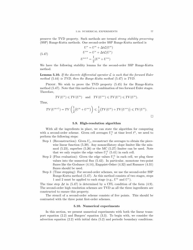
5.10. NUMERICAL EXPERIMENTS 77
preserve the TVD property. Such methods are termed strong stability preserving(SSP) Runge-Kutta methods. One second-order SSP Runge-Kutta method is
(5.47)
U∗ = Un + ∆tL(Un)
U∗∗ = U∗ + ∆tL(U∗)
Un+1 =1
2(Un + U∗∗)
We have the following stability lemma for the second-order SSP Runge-Kuttamethod.
Lemma 5.10. If the discrete differential operator L is such that the forward Eulermethod (5.44) is TVD, then the Runge-Kutta method (5.47) is TVD.
Proof. We wish to prove the TVD property (5.45) for the Runge-Kuttamethod (5.47). Note that this method is a combination of two forward Euler stages.Therefore,
TV (U∗) 6 TV (Un) and TV (U∗∗) 6 TV (U∗) 6 TV (Un).
Thus,
TV (Un+1) = TV
(1
2
(Un + U∗∗
))6
1
2
(TV (Un) + TV (U∗∗)
)6 TV (Un).
5.9. High-resolution algorithm
With all the ingredients in place, we can state the algorithm for computingwith a second-order scheme. Given cell averages Unj at time level tn, we need toperform the following steps:
Step 1 (Reconstruction): Given Uj , reconstruct the averages to obtain the piece-wise linear function (5.39). Any nonoscillatory slope limiter like the min-mod (5.23), superbee (5.26) or the MC (5.27) limiter can be used. Notethat we only require the edge values U±j (5.41) in each cell.
Step 2 (Flux evaluation): Given the edge values U±j in each cell, we plug these
values into the numerical flux (5.42). In particular, monotone two-pointfluxes like the Godunov (4.14), Engquist-Osher (4.32) and Rusanov (4.31)fluxes should be used.
Step 3 (Time stepping): For second-order schemes, we use the second-order SSPRunge-Kutta method (5.47). As this method consists of two stages, steps1 and 2 must be applied to each stage (e.g., Un and U∗).
The time step ∆t in (5.47) is determined by a CFL condition of the form (4.9).The second-order high resolution schemes are TVD as all the three ingredients areconstructed to ensure this property.
The stencil of a second-order scheme consists of five points. This should becontrasted with the three point first-order schemes.
5.10. Numerical experiments
In this section, we present numerical experiments with both the linear trans-port equation (2.2) and Burgers’ equation (3.3). To begin with, we consider theadvection equation (2.2) with initial data (5.2) and periodic boundary conditions.
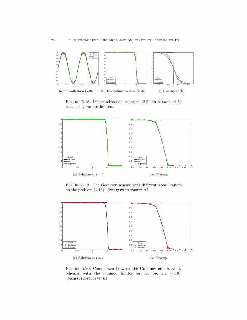
78 5. SECOND-ORDER (HIGH-RESOLUTION) FINITE VOLUME SCHEMES
0 0.2 0.4 0.6 0.8 1−1
−0.8
−0.6
−0.4
−0.2
0
0.2
0.4
0.6
0.8
1
x
ExactMinmodMCSuperbee
(a) Smooth data (5.2).
0 0.5 1 1.5 21
1.1
1.2
1.3
1.4
1.5
1.6
1.7
1.8
1.9
2
x
ExactMinmodMCSuperbee
(b) Discontinuous data (2.26).
1.3 1.35 1.4 1.45 1.5 1.55 1.6 1.65 1.71
1.1
1.2
1.3
1.4
1.5
1.6
1.7
1.8
1.9
2
x
ExactMinmodMCSuperbee
(c) Closeup of (b).
Figure 5.18. Linear advection equation (2.2) on a mesh of 50cells, using various limiters.
−1 −0.5 0 0.5 10
0.1
0.2
0.3
0.4
0.5
0.6
0.7
0.8
0.9
1
x
ExactMinmodMCSuperbee
(a) Solution at t = 1.
0.3 0.35 0.4 0.45 0.5 0.55 0.6 0.65 0.70
0.1
0.2
0.3
0.4
0.5
0.6
0.7
0.8
0.9
1
x
ExactMinmodMCSuperbee
(b) Closeup.
Figure 5.19. The Godunov scheme with different slope limiterson the problem (4.16). [burgers reconstr.m]
−1 −0.5 0 0.5 10
0.1
0.2
0.3
0.4
0.5
0.6
0.7
0.8
0.9
1
x
ExactGodunovRusanov
(a) Solution at t = 1.
0.3 0.35 0.4 0.45 0.5 0.55 0.6 0.65 0.70
0.1
0.2
0.3
0.4
0.5
0.6
0.7
0.8
0.9
1
x
ExactGodunovRusanov
(b) Closeup.
Figure 5.20. Comparison between the Godunov and Rusanovschemes with the minmod limiter on the problem (4.16).[burgers reconstr.m]
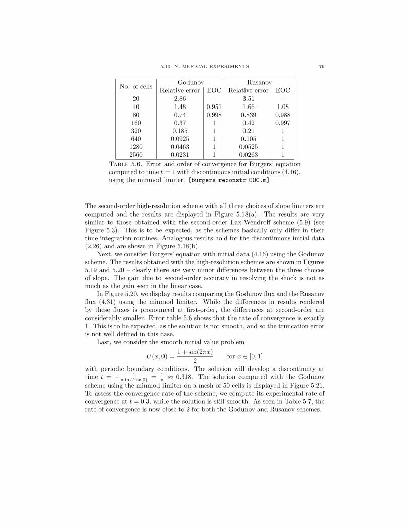
5.10. NUMERICAL EXPERIMENTS 79
No. of cellsGodunov Rusanov
Relative error EOC Relative error EOC20 2.86 – 3.51 –40 1.48 0.951 1.66 1.0880 0.74 0.998 0.839 0.988160 0.37 1 0.42 0.997320 0.185 1 0.21 1640 0.0925 1 0.105 11280 0.0463 1 0.0525 12560 0.0231 1 0.0263 1
Table 5.6. Error and order of convergence for Burgers’ equationcomputed to time t = 1 with discontinuous initial conditions (4.16),using the minmod limiter. [burgers reconstr OOC.m]
The second-order high-resolution scheme with all three choices of slope limiters arecomputed and the results are displayed in Figure 5.18(a). The results are verysimilar to those obtained with the second-order Lax-Wendroff scheme (5.9) (seeFigure 5.3). This is to be expected, as the schemes basically only differ in theirtime integration routines. Analogous results hold for the discontinuous initial data(2.26) and are shown in Figure 5.18(b).
Next, we consider Burgers’ equation with initial data (4.16) using the Godunovscheme. The results obtained with the high-resolution schemes are shown in Figures5.19 and 5.20 – clearly there are very minor differences between the three choicesof slope. The gain due to second-order accuracy in resolving the shock is not asmuch as the gain seen in the linear case.
In Figure 5.20, we display results comparing the Godunov flux and the Rusanovflux (4.31) using the minmod limiter. While the differences in results renderedby these fluxes is pronounced at first-order, the differences at second-order areconsiderably smaller. Error table 5.6 shows that the rate of convergence is exactly1. This is to be expected, as the solution is not smooth, and so the truncation erroris not well defined in this case.
Last, we consider the smooth initial value problem
U(x, 0) =1 + sin(2πx)
2for x ∈ [0, 1]
with periodic boundary conditions. The solution will develop a discontinuity attime t = − 1
minU ′(x,0) = 1π ≈ 0.318. The solution computed with the Godunov
scheme using the minmod limiter on a mesh of 50 cells is displayed in Figure 5.21.To assess the convergence rate of the scheme, we compute its experimental rate ofconvergence at t = 0.3, while the solution is still smooth. As seen in Table 5.7, therate of convergence is now close to 2 for both the Godunov and Rusanov schemes.
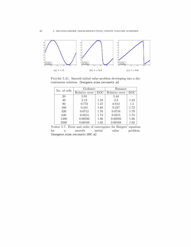
80 5. SECOND-ORDER (HIGH-RESOLUTION) FINITE VOLUME SCHEMES
0 0.2 0.4 0.6 0.8 10
0.1
0.2
0.3
0.4
0.5
0.6
0.7
0.8
0.9
1
x
Exact
Godunov
(a) t = 0
0 0.2 0.4 0.6 0.8 10
0.1
0.2
0.3
0.4
0.5
0.6
0.7
0.8
0.9
1
x
Exact
Godunov
(b) t = 0.3
0 0.2 0.4 0.6 0.8 10
0.1
0.2
0.3
0.4
0.5
0.6
0.7
0.8
0.9
1
x
Exact
Godunov
(c) t = 0.6
Figure 5.21. Smooth initial value problem developing into a dis-continuous solution. [burgers sine reconstr.m]
No. of cellsGodunov Rusanov
Relative error EOC Relative error EOC20 5.01 – 5.44 –40 2.13 1.23 2.3 1.2480 0.772 1.47 0.812 1.5160 0.241 1.68 0.247 1.72320 0.0712 1.76 0.0716 1.79640 0.0214 1.73 0.0215 1.741280 0.00592 1.86 0.00592 1.862560 0.00168 1.82 0.00168 1.82
Table 5.7. Error and order of convergence for Burgers’ equationfor a smooth initial value problem.[burgers sine reconstr OOC.m]
CHAPTER 6
Linear hyperbolic systems in one space dimension
In the last few chapters, we have treated the nonlinear scalar conservation law(3.4) and have designed robust high-order finite volume schemes to approximate itsentropy solutions.
Despite their occurance in many interesting models, scalar conservation lawsare too simplistic to be used for modeling complex physical phenomena as theseproblems involve the interaction of many unknowns. These problems (see Chapter1 for examples) are modeled by a nonlinear system of conservation laws:
(6.1) Ut + f(U)x = 0,
where U = [U1, U2, . . . , Um]> is the vector of unknowns and f = [f1, f2, . . . , fm]>
is the flux vector. Note that (6.1) represents an m×m system of conservation lawsin one space dimension. Multi-dimensional systems will be considered later. Thesystem (6.1) is supplemented with suitable initial and boundary conditions. Whenm = 1, the system reduces to the scalar conservation law (3.4).
To begin with, we consider the simplest case of (6.1) in the form a linear system,
(6.2) Ut +AUx = 0.
Here, A is an m×m matrix with constant (in both space and time) entries. Linearsystems arise for instance when linearizing (6.1) around a constant state U, whichamounts to solving (6.2) with the constant matrix A = ∂f
∂U (U).A related linear system with variable coefficients takes the form
(6.3) Ut + (A(x, t)U)x = 0.
It can be recast into the non-conservative form
(6.4) Ut +A(x, t)Ux = −Ax(x, t)U.
6.1. Examples for linear systems
6.1.1. The wave equation. The simplest example of (6.2) is given by theone-dimensional wave equation,
(6.5) utt − c2uxx = 0.
This equation is also known as the string equation, as it models vibrations inmedia like strings and rods. Its derivation can be found in many text books; see forinstance [10]. The wave equation can be written as a first-order system by definingauxiliary variables v = cux and w = −ut. With this change of variables, it is easyto show that (6.5) transforms to
(6.6)vt + cwx = 0
wt + cvx = 0.
81
82 6. LINEAR HYPERBOLIC SYSTEMS IN ONE SPACE DIMENSION
Hence, the wave equation (6.6) is an example of the linear system (6.2) with
(6.7) U =
[vw
], A =
[0 cc 0
].
6.1.2. Maxwell’s equations. The dynamics of electromagnetic waves is mod-eled by the Maxwell equations of electrodynamics:
(6.8)
Bt + curl(E) = 0
Et − c2curl(B) = − j
ε0
div(B) = 0
div(E) =ρ
ε0.
Here, B = [B1, B2, B3]> and E = [E1, E2, E3]> are the magnetic and electric fields,respectively. The charge and current density are denoted by ρ and j, respectively.The speed of light is given by c2 = µ0ε0, where µ0 and ε0 are constants. In onespace dimension, solving for electromagnetic waves propagating in the x-direction(with no current) reduces (6.8) to
(6.9)B2t + E3
x = 0
E3t + c2B2
x = 0.
Thus, Maxwell’s equations are equivalent to the wave equation (6.7) with U =[cB2, E3]>, leading to another concrete application of the wave equation.
6.1.3. Linearized Euler equations. The Euler equations of gas dynamics(1.10) are a nonlinear system of conservation laws in several spatial dimensions.Let ρ, u and p denote the density, velocity and pressure of the gas, respectively.Restricting the equations to one space dimension and linearizing (1.10) around aconstant state U = [ρ, u, p]>, we obtain the linearized Euler equations,
(6.10)
ρt + uρx + ρux = 0
ut + uux +1
ρpx = 0
pt + γpux + upx = 0.
This system of equations can be written as a linear system (6.2) with
(6.11) U =
ρup
, A =
u ρ 00 u 1
ρ
0 γp u
.The linearized Euler equations are a good approximation of the more complex Eulerequations (1.10) when the solution only consists of small perturbations aroundconstant states.
Given the above examples, the study of the linear system (6.2) is importantin its own right. Furthermore, it serves as an example of the nonlinear system(6.1), and so the study of the linear system will be a starting point in the design ofefficient numerical schemes for approximating (6.1).
6.2. HYPERBOLICITY AND CHARACTERISTIC DECOMPOSITION 83
6.2. Hyperbolicity and characteristic decomposition
We will consider the initial value problem associated with (6.2) by augmentingit with initial data
U(x, 0) = U0(x).
One of the key notions underlying the behavior of the solutions of (6.2) is theconcept of hyperbolicity. For scalar equations, the notion of hyperbolicity referredto the property of finite speed of propagation. Such a notion will hold true for asystem.
Definition 6.1 (Hyperbolic system). The linear system (6.2) is hyperbolic if thematrix A is diagonalizable and has m real eigenvalues. Similarly, the equation (6.3)is hyperbolic if the matrix A(x, t) is diagonalizable and has m real eigenvalues forall x, t. Both systems are termed strictly hyperbolic if the eigenvalues are distinct.
Thus, the concept of hyperbolicity for a system is tied to the eigenstructure ofthe underlying matrix. Why is the eigenstructure linked to finite speed of prop-agation? The answers lies in diagonalizability. A matrix A is diagonalizable if ithas a complete set of eigenvectors, i.e, there exists m linearly independent vectorsr1, . . . , rm ∈ Rm and corresponding eigenvalues λ1, . . . , λm ∈ R such that
Arp = λprp.
We can then define the matrix of eigenvectors
(6.12) R = [r1|r2| · · · |rm]
and the diagonal matrix of eigenvalues
(6.13) Λ = diag (λ1, . . . , λm)
and use them to diagonalize the underlying matrix A – that is, write it in the form
(6.14) A = RΛR−1.
The diagonalization of A leads us to the following decoupling:
Ut +AUx = 0
Ut +RΛR−1Ux = 0 (from (6.14))
Ut +RΛ(R−1U
)x
= 0 (constant coefficient)(R−1U
)t
+R−1RΛ(R−1U
)x
= 0 (multiplying both sides with R−1)(R−1U
)t
+ Λ(R−1U
)x
= 0.
Introducing the vector of characteristic variables
V = R−1U,
the above calculation leads to
(6.15) Vt + ΛVx = 0.
Thus, the hyperbolic linear system (6.2) is completely decoupled into a set of scalarlinear transport equations, obtained by writing (6.15) componentwise:
(6.16) V pt + λpVpx = 0 for p = 1, . . . ,m,
84 6. LINEAR HYPERBOLIC SYSTEMS IN ONE SPACE DIMENSION
where V p(x, t) is the p-th component of V(x, t). This decoupled set of transportequations can be solved explicitly by the method of characteristics (see Chapter 2)to obtain
(6.17) V p(x, t) = W p0 (x− λpt) ,
where
V0(x) = R−1U0(x)
and again W p0 (x, t) is the p-th component of V0(x, t). Therefore, we can explicitly
write the initial value problem for a hyperbolic system (6.2) as
(6.18) U(x, t) = RV(x, t).
6.3. Solutions of Riemann problems, waves
We illustrate the explicit solution (6.18) for the Riemann initial data
(6.19) U0(x) =
UL if x < 0
UR if x > 0.
The first step in finding an explicit solution is to determine Λ and R for the givensystem A. These are used to define V0 = R−1U0, which will be of the form
V0(x) =
VL if x < 0
VR if x > 0.
with VL = R−1UL and VR = R−1UR. Then we can solve (6.16) in terms of thetransport equation (6.17) to obtain
V p(x, t) =
V pL if x < λpt
V pR if x > λpt.
The solution U is obtained by letting U = RV. This solution consists of m waves,one for each eigenvector. The p-th wave propagates with a speed of λp, and acrossthis wave, there is a jump in only the p-th component of V. This is seen clearly bydecomposing the jump UR −UL in terms of eigenvectors:
UR −UL = R (VR −VL)
=
m∑p=1
(V pR − VpL ) rp
=
m∑p=1
αprp,
(6.20)
where αp := V pR − V pL is the wave strength of the p-th wave. Hence, the jumpacross the p-th wave is proportional to the eigenvector rp. Thus, the solution of theRiemann problem for a linear system corresponds to decomposing the initial jumpinto m waves (with the corresponding eigenvalue being the wave speed), with thejump across the p-th wave being proportional to the corresponding eigenvector.
6.4. FINITE VOLUME SCHEMES 85
6.3.1. Example: The wave equation. We consider the linear wave equation(6.6). It is straightforward to find that the eigenvalues and eigenvectors of A are
(6.21) Λ = diag(−c, c), R =
[−1 11 1
], R−1 =
[− 1
212
12
12
].
Thus, the wave equation is strictly hyperbolic and diagonalizable, so the aboveconstruction of the explicit solution is applicable. Consider the Riemann problem(6.19) for the wave equation (6.6). Let c = 1 for simplicity. The solution of theRiemann problem is then
(6.22) U(x, t) =
UL if x < −tU∗ if − t < x < t
UR if x > t,
where the mid-state U∗ is given by
U∗ = R
[vR−uR
2vL+uL
2
].
Thus, it is straightforward to calculate solutions to the Riemann problem for thewave equation.
6.3.2. Example: Linearized Euler equations. The eigenstructure of thelinearized Euler equations (6.10) can be explicit computed as
(6.23) Λ = diag (u− a, u, u+ a) , R =
− ρa 1 ρa
1 0 1−ρa 0 ρa
,where
a =
√γp
ρ
denotes the local sound speed. Hence, the linearized Euler equations are strictlyhyperbolic. The two waves corresponding to r1 and r3 are termed the acousticor sound waves and the wave corresponding to r2 is called a contact wave. TheRiemann problem for the linearized Euler equations can be solved explicitly withthe procedure outlined above.
6.4. Finite volume schemes
In this section, we construct finite volume schemes to approximate the linearsystem (6.2). For simplicity, we consider a uniform grid in both space and timewith mesh size ∆x and time step ∆t. The mesh size and time step are related viaa CFL type condition to be specified in the sequel. We denote the grid points asxj+1/2 = xL + (j + 1/2)∆x and the time levels by tn. The domain is divided intocells denoted by
Cj = [xj+1/2, xj−1/2).
See Figure 4.1 for an illustration of the grid.By now, we are familiar with the design procedure (see Chapter 4) and know
that it consists of the following steps:
86 6. LINEAR HYPERBOLIC SYSTEMS IN ONE SPACE DIMENSION
(i) Reconstruction: If the solution U is known at a certain time level tn,we evaluate its cell averages Un
j as
Unj =
1
∆x
∫ x+1/2
x−1/2
U(x, tn)dx.
(ii) Evolution: The reconstruction procedure projects the solution into thespace of piecewise constant functions and leads to a superposition of theRiemann problems
(6.24)
Ut +AUx = 0
U(xj+1/2, tn) =
Unj if xj < x < xj+1/2,
Unj+1 if xj+1/2 < x < xj+1
at each interface xj+1/2. These Riemann problems can be solved exactly(as described in the previous section) or approximately (see the sequel).
We know that the fastest wave speed for each problem is bounded bythe modulus of the maximum eigenvalue,
λmax = max16p6m
|λp|,
where λp is the p-th eigenvalue of A. Hence, imposing a CFL condition
(6.25) λmax∆t
∆x6
1
2
prevents the waves from the neighboring problems to interact before timelevel tn+1.
(iii) Averaging: The solution of (6.24) is averaged over each cell to obtainUn+1j . The cell average can be explicitly computed by integrating (6.24)
over Cj × [tn, tn+1). This gives the finite volume scheme
(6.26) Un+1j = Un
j −∆t
∆x
(Fnj+1/2 − Fnj−1/2
)with
(6.27) Fnj+1/2 = F(Unj ,U
nj+1
):= AUj+1/2(xj+1/2, 0).
Here, Uj+1/2 is the solution of the (exact or approximate) solution of theRiemann problem (6.24). We remark that the solution is self-similar andits value at the interface is time independent.
The finite volume scheme (6.26) is similar to the scheme for scalar equations.The only difference lies in the more complicated structure of solutions of the Rie-mann problem (6.24). We need to complete (6.26) by computing the numerical fluxexplicitly.
6.4.1. Godunov flux. The Riemann problem (6.24) can be solved explicitlyas described before. The resulting flux evaluation (6.27) defines the Godunov fluxfor the linear system (6.2). It turns out that we can derive a neat expression forthe Godunov flux.
Let a+ = max(a, 0) and a− = min(a, 0). Then a = a++a− and |a| = a+−a− forany a ∈ R. The explicit solution of the Riemann problem (6.24) can be computed
6.4. FINITE VOLUME SCHEMES 87
and the interface value Uj+1/2(xj+1/2, 0) = U∗ can be calculated (see (6.20)) by
(6.28) U∗ = Unj +
∑p:λp<0
αpj+1/2rp,
where αpj+1/2 is the wave strength of the p-th wave, given by the p-th component of
R−1(Unj+1−Un
j ). Since we are interested in calculating the interface flux in (6.27),we multiply both sides of (6.28) by A to obtain
(6.29)
AU∗ = AUnj +A
( ∑p:λp<0
αpj+1/2rp
)= AUn
j +∑
p:λp<0
αpj+1/2Arp
= AUnj +
∑p:λp<0
αpj+1/2λprp (as rp are eigenvectors of A)
= AUnj +
∑p
λ−p αpj+1/2rp.
Similarly, we have
U∗ = Unj+1 −
∑p:λp>0
αpj+1/2rp.
Repeating the calculations of (6.29), we obtain
(6.30) AU∗ = AUnj+1 −
∑p
λ+p α
pj+1/2rp.
Taking the average of (6.29) and (6.30) leads to
(6.31)
AU∗ =1
2
(AUn
j +AUnj+1 −
∑p
(λ+p − λ−p )αpj+1/2rp
)
=1
2A(Unj + Un
j+1
)− 1
2
∑p
|λp|αpj+1/2rp.
Using the definition of the wave strength αpj+1/2 and defining
|Λ| = diag(|λ1|, · · · , |λm|),
it is straightforward to rewrite (6.31) as
(6.32) Fnj+1/2 = AU∗ =1
2A(Unj + Un
j+1
)− 1
2R|Λ|R−1
(Unj+1 −Un
j
).
This is the explicit form of the Godunov flux for a linear system.The Godunov scheme (6.26) with flux (6.32) for the linear system (6.2) should
be compared with the upwind flux (2.17) for the linear transport equation (2.2). Inparticular, both fluxes are written in the central + diffusion form. The upwindingfor a system is more complicated and involves characteristic decomposition. Notethat the flux (6.32) reduces to the standard upwind flux for a scalar equation, whenm = 1.
88 6. LINEAR HYPERBOLIC SYSTEMS IN ONE SPACE DIMENSION
6.4.2. Lax-Friedrichs and Rusanov flux. The Godunov flux (6.32) re-quires a characteristic decomposition of the system. Explicit expressions for theeigenvalues and eigenvectors may not be available in some cases, and in others itmight be computationally costly to evaluate them. Hence, there is scope for design-ing cheaper alternative numerical fluxes that are easy to implement. ApproximateRiemann solvers (see Chapter 4) provide a recipe for designing such fluxes. Thekey idea is to replace the exact solution of the Riemann problem (6.24) with anapproximate solution. The Lax-Friedrichs flux is based on a two-wave approximateRiemann solver (see Section 4.2.2). It is straightforward to generalize it to thecase of a linear system: We replace the exact solution (consisting of m waves) withexactly two waves, one moving to the left and another to the right (see Figure 4.7).The wave speeds are − ∆x
2∆t and ∆x2∆t , which is the maximum possible wave speed
consistent with the CFL condition (6.25). The resulting flux is
(6.33) Fnj+1/2 = FLxF(Unj ,U
nj+1
)=
1
2A(Unj + Un
j+1
)− ∆x
2∆t
(Unj+1 −Un
j
).
(compare to (4.29)). This flux is trivial to implement as it does not require anycharacteristic information.
As in the scalar case, the Lax-Friedrichs scheme ((6.26) with (6.33)) is likely tobe diffusive. A more reasonable choice of wave speeds in the approximate Riemannsolver is the largest eigenvalue of A. (Note that the maximum wave speed in theRiemann problem (6.24) is always bounded by the maximum eigenvalue of A.) Theresulting flux is the Rusanov flux
(6.34) Fnj+1/2 = FRus(Unj ,U
nj+1
)=
1
2A(Unj + Un
j+1
)− λmax
2
(Unj+1 −Un
j
)(compare to (4.31)). The only characteristic information used in the Rusanovscheme is an estimate on the maximum eigenvalue of A.
6.5. Numerical experiments
In this section we present numerical experiments for linear systems (6.2) usingthe Godunov, Lax-Friedrichs and Rusanov schemes.
6.5.1. Numerical experiment 1. Consider the wave equation (6.6) withwave speed c = 1. Let the initial data be the Riemann problem
u0(x) =
1− cos2(2π(x− 0.25)) if 0.25 6 x 6 0.75
0 otherwise
v0(x) = 0.
(6.35)
We compute on the periodic domain x ∈ [−1, 1] and divide the domain into 100grid cells. In Figure 6.1 we present the computational results with the Godunov,Lax-Friedrichs and Rusanov schemes at time t = 0.5, 1 and 2. The initial profilefor u first separates into two parts, and at time t = 1 they meat at x = −0.5 andmerge together. This process is again repeated at time t = 2, at which time thesolution is the same as at t = 0.
From Figure 6.1 it is clear that the Lax-Friedrichs scheme is more diffusivethan the Godunov and Rusanov schemes. On the other hand, the Godunov andRusanov schemes produce an identical profile. The reason for this is that in thiscase the Rusanov and Godunov schemes are identical.
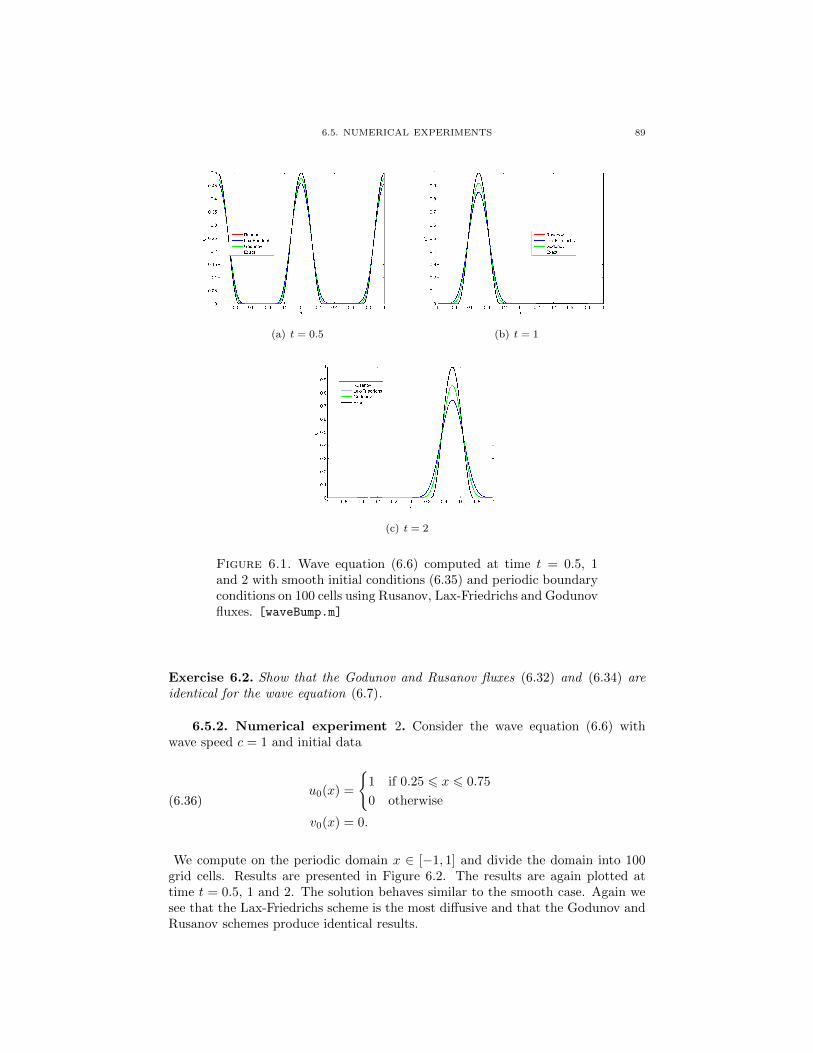
6.5. NUMERICAL EXPERIMENTS 89
(a) t = 0.5 (b) t = 1
(c) t = 2
Figure 6.1. Wave equation (6.6) computed at time t = 0.5, 1and 2 with smooth initial conditions (6.35) and periodic boundaryconditions on 100 cells using Rusanov, Lax-Friedrichs and Godunovfluxes. [waveBump.m]
Exercise 6.2. Show that the Godunov and Rusanov fluxes (6.32) and (6.34) areidentical for the wave equation (6.7).
6.5.2. Numerical experiment 2. Consider the wave equation (6.6) withwave speed c = 1 and initial data
u0(x) =
1 if 0.25 6 x 6 0.75
0 otherwise
v0(x) = 0.
(6.36)
We compute on the periodic domain x ∈ [−1, 1] and divide the domain into 100grid cells. Results are presented in Figure 6.2. The results are again plotted attime t = 0.5, 1 and 2. The solution behaves similar to the smooth case. Again wesee that the Lax-Friedrichs scheme is the most diffusive and that the Godunov andRusanov schemes produce identical results.
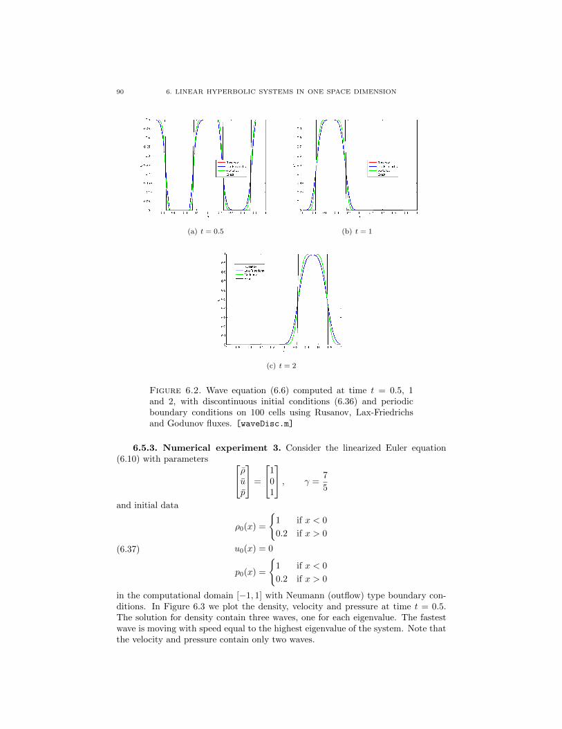
90 6. LINEAR HYPERBOLIC SYSTEMS IN ONE SPACE DIMENSION
(a) t = 0.5 (b) t = 1
(c) t = 2
Figure 6.2. Wave equation (6.6) computed at time t = 0.5, 1and 2, with discontinuous initial conditions (6.36) and periodicboundary conditions on 100 cells using Rusanov, Lax-Friedrichsand Godunov fluxes. [waveDisc.m]
6.5.3. Numerical experiment 3. Consider the linearized Euler equation(6.10) with parameters ρu
p
=
101
, γ =7
5
and initial data
ρ0(x) =
1 if x < 0
0.2 if x > 0
u0(x) = 0
p0(x) =
1 if x < 0
0.2 if x > 0
(6.37)
in the computational domain [−1, 1] with Neumann (outflow) type boundary con-ditions. In Figure 6.3 we plot the density, velocity and pressure at time t = 0.5.The solution for density contain three waves, one for each eigenvalue. The fastestwave is moving with speed equal to the highest eigenvalue of the system. Note thatthe velocity and pressure contain only two waves.
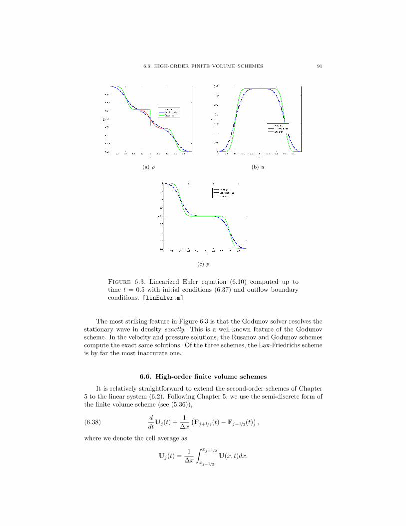
6.6. HIGH-ORDER FINITE VOLUME SCHEMES 91
(a) ρ (b) u
(c) p
Figure 6.3. Linearized Euler equation (6.10) computed up totime t = 0.5 with initial conditions (6.37) and outflow boundaryconditions. [linEuler.m]
The most striking feature in Figure 6.3 is that the Godunov solver resolves thestationary wave in density exactly. This is a well-known feature of the Godunovscheme. In the velocity and pressure solutions, the Rusanov and Godunov schemescompute the exact same solutions. Of the three schemes, the Lax-Friedrichs schemeis by far the most inaccurate one.
6.6. High-order finite volume schemes
It is relatively straightforward to extend the second-order schemes of Chapter5 to the linear system (6.2). Following Chapter 5, we use the semi-discrete form ofthe finite volume scheme (see (5.36)),
(6.38)d
dtUj(t) +
1
∆x
(Fj+1/2(t)− Fj−1/2(t)
),
where we denote the cell average as
Uj(t) =1
∆x
∫ xj+1/2
xj−1/2
U(x, t)dx.
92 6. LINEAR HYPERBOLIC SYSTEMS IN ONE SPACE DIMENSION
Given cell averages Uj , we wish to obtain a linear reconstruction pj in each cell Cjof the form
(6.39) pj(x) = Uj + σj(x− xj).These linear functions are combined to form the piecewise linear function
(6.40) p(x, t) = pj(x) for xj−1/2 6 x < xj+1/2.
Contrary to the situation in Chapter 5, the slope σj is now a vector, and so thetheory for scalar equations does not translate directly to the present situation.There are two basic approaches to constructing the slope σj .
6.6.1. Reconstruction in primitive variables. One approach to construct-ing σj is to reconstruct in primitive (conserved) variables Upj (p = 1, . . . ,m). Thisinvolves applying the reconstruction procedures of Chapter 5 to each component ofUj , thus constructing σj component by component.
6.6.2. Reconstruction in characteristic variables. An alternative recon-struction involves using the characteristic variables. Given the cell averages Uj ,we define the corresponding characteristic average Vj = R−1Uj . We can thenperform a componentwise reconstruction in Vj , as outlined in the previous section,to obtain a reconstruction
(6.41) Vj(x) = Vj + µj(x− xj).The primitive variables are then obtained from
(6.42) pj(x) = RVj(x).
6.6.3. The numerical flux. As in the scalar case, the numerical flux F in(6.38) is defined by
(6.43) Fj+1/2 = F(U+j ,U
−j+1
),
where
(6.44) U+j = pj(xj+1/2), U−j = pj(xj−1/2),
and F is either the Godunov (6.32), Lax-Friedrichs (6.33) or Rusanov (6.34) nu-merical flux.
6.6.4. Time stepping. The time integration for (6.38) is performed with anSSP Runge-Kutta method, as described in Chapter 5. Denoting
U(t) = [. . . ,Uj−1(t),Uj(t),Uj+1(t), . . . ],
the finite volume scheme (6.38) can be rewritten as
(6.45)d
dtU(t) = L(U(t)),
where the operator L acts pointwise on the vector U as
L(U(t))j := − 1
∆x
(Fj+1/2(t)− Fj−1/2(t)
).
The second-order SSP Runge-Kutta method is then defined by
(6.46)
U∗ = Un + ∆tL(Un)
U∗∗ = U∗ + ∆tL(U∗)
Un+1 =1
2(Un + U∗∗).
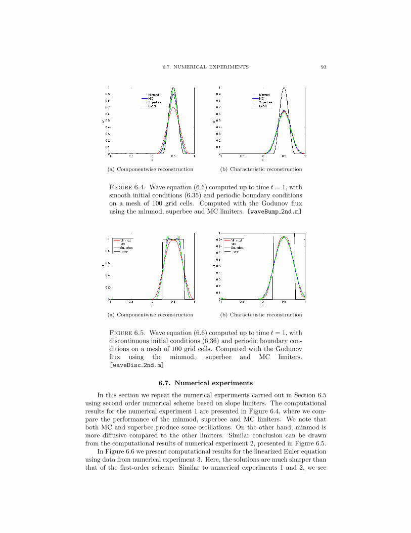
6.7. NUMERICAL EXPERIMENTS 93
(a) Componentwise reconstruction (b) Characteristic reconstruction
Figure 6.4. Wave equation (6.6) computed up to time t = 1, withsmooth initial conditions (6.35) and periodic boundary conditionson a mesh of 100 grid cells. Computed with the Godunov fluxusing the minmod, superbee and MC limiters. [waveBump 2nd.m]
(a) Componentwise reconstruction (b) Characteristic reconstruction
Figure 6.5. Wave equation (6.6) computed up to time t = 1, withdiscontinuous initial conditions (6.36) and periodic boundary con-ditions on a mesh of 100 grid cells. Computed with the Godunovflux using the minmod, superbee and MC limiters.[waveDisc 2nd.m]
6.7. Numerical experiments
In this section we repeat the numerical experiments carried out in Section 6.5using second order numerical scheme based on slope limiters. The computationalresults for the numerical experiment 1 are presented in Figure 6.4, where we com-pare the performance of the minmod, superbee and MC limiters. We note thatboth MC and superbee produce some oscillations. On the other hand, minmod ismore diffusive compared to the other limiters. Similar conclusion can be drawnfrom the computational results of numerical experiment 2, presented in Figure 6.5.
In Figure 6.6 we present computational results for the linearized Euler equationusing data from numerical experiment 3. Here, the solutions are much sharper thanthat of the first-order scheme. Similar to numerical experiments 1 and 2, we see
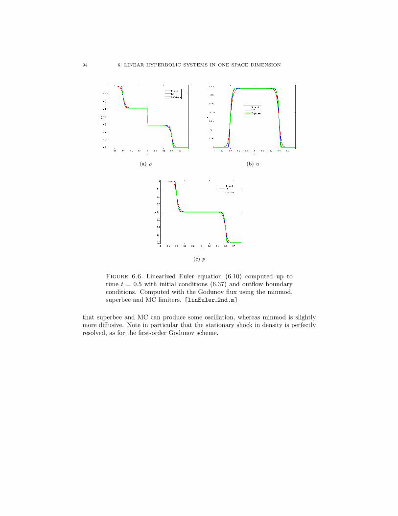
94 6. LINEAR HYPERBOLIC SYSTEMS IN ONE SPACE DIMENSION
(a) ρ (b) u
(c) p
Figure 6.6. Linearized Euler equation (6.10) computed up totime t = 0.5 with initial conditions (6.37) and outflow boundaryconditions. Computed with the Godunov flux using the minmod,superbee and MC limiters. [linEuler 2nd.m]
that superbee and MC can produce some oscillation, whereas minmod is slightlymore diffusive. Note in particular that the stationary shock in density is perfectlyresolved, as for the first-order Godunov scheme.
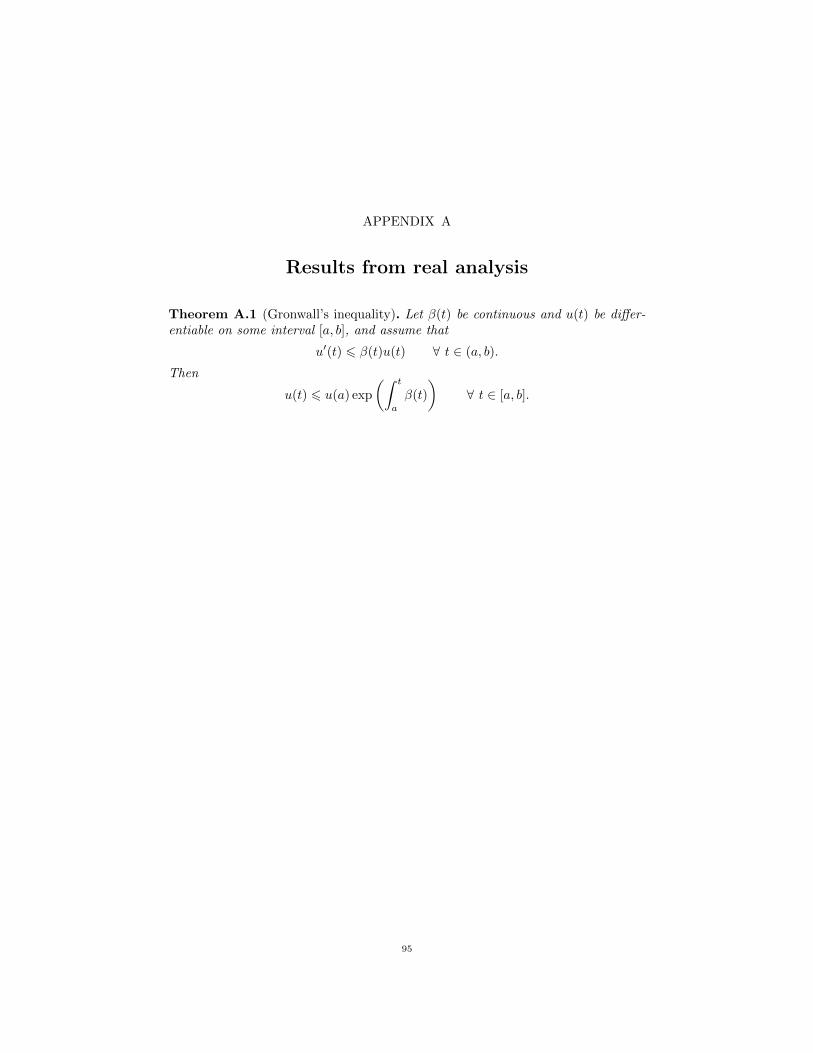
APPENDIX A
Results from real analysis
Theorem A.1 (Gronwall’s inequality). Let β(t) be continuous and u(t) be differ-entiable on some interval [a, b], and assume that
u′(t) 6 β(t)u(t) ∀ t ∈ (a, b).
Then
u(t) 6 u(a) exp
(∫ t
a
β(t)
)∀ t ∈ [a, b].
95

Bibliography
1. E. Godlewski and P.A. Raviart, Hyperbolic systems of conservation laws, Ellipses, 1991.
2. S. K. Godunov, A difference scheme for numerical solution of discontinuous solution of hy-drodynamic equations, Math. Sbornik 47 (1959), 271–306.
3. Sigal Gottlieb, Chi-Wang Shu, and Eitan Tadmor, Strong stability-preserving high-order time
discretization methods, SIAM Review 43 (2001), no. 1, 89–112.4. Ernst Hairer, Syvert P. Nørsett, and Gerhard Wanner, Solving ordinary differential equations,
1987.
5. A. Harten, S. Osher, B. Engquist, and S. R. Chakravarthy, Some results on uniformly high-order accurate essentially nonoscillatory schemes, Appl. Numer. Math. 2 (1986), no. 3-5,
347–378.6. S N Kruzkov, First order quasilinear equations in several independent variables, Mathematics
of the USSR-Sbornik 10 (1970), no. 2, 217–243.
7. L. D. Landau and E. M. Lifschitz, Fluid mechanics, Butterworth-Heinemann, 1987.8. Xu-Dong Liu, Stanley Osher, and Tony Chan, Weighted essentially non-oscillatory schemes,
J. Comput. Phys. 115 (1994), no. 1, 200–212.
9. C.-W. Shu, Essentially non-oscillatory and weighted essentially non-oscillatory schemes forhyperbolic conservation laws, Tech. report, 1997.
10. Aslak Tveito and Ragnar Winther, Introduction to partial differential equations; a computa-
tional approach, second ed., vol. 29, Springer-Verlag, 2009, 392 pages.
97