numerical methods for identification of induction motor
TRANSCRIPT

Numerical Methods for Identification of Induction
Motor Parameters
by
Steven Robert Shaw
S.B. Massachusetts Institute of Technology (1995)
Submitted to the Department of Electrical Engineering and ComputerScience
in partial fulfillment of the requirements for the degrees of
Master of Engineering in Electrical Engineering and Computer Science
and
Electrical Engineer
at the
MASSACHUSETTS INSTITUTE OF TECHNOLOGY
February 1997
@ Massachusetts Institute of Technology 1997. All rights reserved.
OCT 291991Author..
Department of Electrical Engineering and Computer Science
Certified by
January 24, 1997
Steven B. Leeb;sistant Professor'hesis Supervisor
A I
Accepted by .Arthur C. Smith
Chairman, Departmenta\ Committee on: Graduate Theses

Numerical Methods for Identification of Induction Motor
Parameters
by
Steven Robert Shaw
Submitted to the Department of Electrical Engineering and Computer Scienceon January 24, 1997, in partial fulfillment of the
requirements for the degrees ofMaster of Engineering in Electrical Engineering and Computer Science
andElectrical Engineer
Abstract
This thesis presents two methods for determining the parameters of a lumped inductionmotor model given stator current and voltage measurements during a startup transient.The first method extrapolates a series of biased parameter estimates obtained fromreduced order models to an unbiased estimate using rational functions. The secondmethod uses part of the lumped parameter model as a rotor current estimator. Theestimated rotor currents are used to identify the mechanical subsystem and to predictthe rotor voltages. Errors in the predicted rotor voltages are minimized using standardnon-linear least squares techniques. Both methods are demonstrated on simulated andmeasured induction motor transient data.
Thesis Supervisor: Steven B. LeebTitle: Assistant Professor

Acknowledgments
I would like to thank Professor Steven Leeb for his support, guidance and patience.
Professor Leeb's enthusiasm is both unwavering and inspiring.
Tektronix and Intel generously donated equipment essential to this work.
This project was supported by ORD/EPG and Lincoln Labs, ACC Project No.
182A administered by Marc Bernstein.

Contents
1 Introduction
1.1 Thesis Outline . ............
1.2 Overview of related work .......
1.3 Methods for system identification
1.3.1 Linear least squares ......
1.3.2 Weighted least squares .
1.3.3 Numerical methods for finding
1.3.4 Non-linear least squares
1.4 Discrete time identification ......
1.5 Continuous time identification .
1.5.1 Identification of an RC Circuit
1.5.2 Computation of A .......
1.6 Summary ...............
(ATA) - 1
from samples of the step response
2 Induction Motor Model
2.1 Arbitrary reference frame transformations ...............
2.2 Model of Induction Motor (After Krause) . ...............
2.3 Induction Machine Equations in Complex Variables ..........
2.4 Simulation of Induction Motor Model . .................
3 Extrapolative System Identification
3.1 Rational function extrapolation .....................
3.2 RC Example ................................

3.3 Simplified induction motor models ................... . 54
3.3.1 Model for high slip ................... ..... 54
3.3.2 Model for low slip . ................ . ... ... . 55
3.4 Summary ....................... . . . . . 56
4 Modified Least Squares 57
4.1 Eliminating the rotor currents ................... .. . 58
4.2 Rotor current observer ............. . . .. . . . . . 59
4.3 The loss function ........... .. ............... . 60
4.3.1 Spectral Leakage .............. .. . . . . . 62
4.3.2 Partial Derivatives .............. ...... ... .63
4.4 The mechanical interaction . ................. . . ... . 65
4.4.1 Slip estimation by reparametrization and shooting ....... 65
4.4.2 The general case ............. . . . . . . . . 67
4.5 Summary ...... .. .. ..... . . . .. .... ......... 67
5 Results 70
5.1 Simulated data .................................. .... 70
5.1.1 Extrapolative method ... . . . . . . . . . . . . ........ 72
5.1.2 Modified least-squares method ......... . . . . 72
5.2 Measured Data ................................ .... 73
5.2.1 Extrapolative method ........... . . . . . . .. .. 76
5.2.2 Modified least-squares method ........... . . . . . . . 77
6 Conclusions 83
6.1 Extrapolative method ............. . . . . . . .. . . . . . . 83
6.2 Modified least squares ........ . . .. . . . . . . . . ...... . . 84
A Power quality prediction 86
A.1 Power Quality Prediction . . ............ . ........... . 86
A.1.1 Background ......... . .. ........ .... ... 86
A.1.2 Service Model ............ . . .......... .. . 88

A.1.3 DESIRE Prototype ................... .. . . 89
A.1.4 Parameter Estimation and Extrapolation . ........... 90
A.1.5 Identification of the parameters R and L . ........... 90
A.1.6 Estimating transient frequency . .............. . . 92
A.1.7 Frequency dependence of R . .................. 93
A.1.8 Experimental Results ................... .... 94
A.1.9 Conclusions ....... ........... ......... 96
A.2 MATLAB Source Code ......................... 97
B CSIM Simulation Environment 105
B.1 Introduction ...................... ........... 105
B.2 General description of the integration procedure . ........... 106
B.3 A physical description of a lightbulb . .................. 106
B.4 C Code ......................... .......... 107
B.5 Make File ...... . ......... .... .......... 114
B.6 Results ........ ... .. ..... ......... 115
B.7 lightbulb.c ................... ............. 117
B.8 Integration and Utility Codes ................... ... 121
C Simulators 138
C.1 Simulator, Chapter 2 ................. ........ .. 138
C.2 Simulator, Chapter 5 ................... ........ 145
D Extrapolative Identification Code 151
E Modified Least Squares Code 159
E.1 identify.cc ........ .... ...... .......... 159
E.2 estimate.cc ................... ............ 169
F General purpose codes 183
F.1 fourier.cc .............. .... . ............ 183
F.2 lambda.cc ....... .... ... . ....... .. . ....... 188

F.3 mrqmin.cc . ............ .. ... ... ........ 191
F.4 sysidtools.cc ........... ...... ............ 196
F.5 tools.cc ................... .............. 200
F.6 window.cc .......... ... ................ 209
G Data file tools 212
G.1 BASH Script to translate Tektronix .wfm files to .dqo files ...... 212
G.2 File manipulation utilities ................... ..... 213

List of Figures
1-1 Context of the non-intrusive diagnostic system.
1-2 RC circuit for system identification
2-1
2-2
2-3
2-4
2-5
2-6
2-7
3-1
3-2
3-3
3-4
3-5
Induction motor circuit model.
Motor starting transient, iq .
Motor starting transient, ids
Motor starting transient, ia
Motor starting transient, ib
Motor starting transient, i . .
Motor starting transient, s
Phase space illustration of model decomposition . . . . . .
Tangent line model of a circle. . . . . . . . . . ..
Parameterization in the neighborhood of uk. . . . . . . . .
Extrapolation to an unbiased estimated . . . . . . . . . .
Truncated Taylor series and rational approximations to e- t .
3-6 A sequence of fits of the "low-time" model to an RC transient.
3-7 Extrapolation of the unbiased estimates R(0) and C(0) from estimates
at - = 1, 2, 4................................
4-1
4-2
4-3
4-4
Sources of error in the frequency domain . . . . . . . . . . . .
Errors are minimized in a selected band . . . . . . . . . . ...
Blackman window . . . . . . . . . . . . . . . ..
Schematic diagram of modified least squares method . . . . .
. . . . . . . . . . . . 37
. . . . . . . . . 42
.. . . . . . . . 42
. . . . . . . . . . . . 43
.. . . . . . 43
. . . . . . . . . . . . 44
.. . . . . . . 44
.. . . . 46
. . . . . . 47
. . . . . . 47
. . . . . . 48
. . . . . . 50
. . . . 61
. . . . 61
. . . . 62
. . . . 68
5-1 Composite plot of slip and current transients for test motors. .
5-2 Current and voltage measurements in dqO frame, unloaded motor.
5-3 Comparison of simulated and measured transients.
Estimated slip, modified least-squares method. .
Comparison of measured and simulated dq currents.
Utility model.............. ... ...
DESIRE hardware ...... .. . .....
Screen interaction with DESIRE prototype .
Resistance R as a function of frequency f .
Sample current transient . . . . . . . . . . . . .
Measured and predicted line voltage distortion..
B-1 Simulated light bulb current . .........
B-2 Simulated light bulb temperature . . . . . . .
. . . . . 78
5-4
5-5
A-1
A-2
A-3
A-4
A-5
A-6
.... .. 88
.. .... ... . 89
. . . . . . . . . 92
. . . . . . . . . . 95
. . . . . . . . . . 96
. . . . . . . . . . . . 97
115
116

List of Tables
5.1 Extrapolative method estimates, simulated data. . ............ 72
5.2 Modified least-squares method, simulated data . ............ 73
5.3 Boiler-plate data from test induction motor . .............. 74

Chapter 1
Introduction
This work describes numerical techniques for finding the lumped circuit model para-
meters of an induction motor from its electrical startup transient. This work is mo-
tivated by the desire to add diagnostic capabilities to the non-intrusive load monitor
(NILM) developed in [12],[13],[14]. The NILM can detect the operation of electrical
loads in a building by making measurements at the electric utility service entry of a
building. By combining system identification capabilities with the transient recogni-
tion and acquisition ability of the NILM, a non-intrusive diagnostic system might be
possible. The situation is indicated schematically in Figure 1-1.
The premise of non-intrusive diagnostics is that pending problems in electrical
loads manifest themselves in the electrical startup transient detected by the NILM. If
electrical transients could be interpreted in terms of parameters of a physical model,
then the cause of the impending failure might be identified. For example, a cracking
rotor bar in an induction motor would correspond to an increasing rotor resistance,
which might be detected from the startup transient of the defective motor [5],[32]. As
a first step in adding non-intrusive diagnostics to the NILM, this thesis considers the
problem of identifying the parameters of an induction motor from an observed startup
transient.
This thesis develops two methods for determining induction motor parameters. The
first is an extrapolative technique employing reduced order models. The extrapolative
method is philosophically similar to Richardson extrapolation or Stoer-Bulirsch integ-

Motors
Buili
ýuality Survey:hedulingI of Power Quality Offenderss of Power Consumption
on of Systems Failure
Figure 1-1: Context of the non-intrusive diagnostic system.
ration, in that the bias in a series of estimates is extrapolated to zero. The second
method is a more classically oriented modified least-squares method using an observer
extracted from the model. Both of these methods assume the lumped parameter in-
duction motor model introduced by Krause in [11].
1.1 Thesis Outline
This chapter is an brief summary of some of the existing work relevant to induction
motor identification and a review of some essential issues in system identification.
The mathematical framework on which Chapters 3 and 4 are built is presented here,
beginning with a practical discussion of least squares. Methods for solving discrete and
continuous time system identification problems are discussed next, using examples.
In Appendix A, the tools presented are put to work in a detailed example of power
quality prediction based on modeling, identification, and simulation of the electric
utility.
In Chapter 2, arbitrary reference frame transformations and the induction motor

model given in [11] are introduced. Alternate forms of the induction motor model,
useful in the later chapters, are also presented. Simulation of the induction motor
model is considered, and plots of simulated induction motor transients are given.
Source codes for induction motor simulation are listed in Appendices B and C.
In Chapter 3, the extrapolative system identification procedure is developed as
means of obtaining quick estimates of the parameters of a complicated system. Re-
duced order models are selectively applied to the data, and rational functions are used
to extrapolate to approximately unbiased estimates. Source code for the extrapolative
method can be found in Appendix D.
Chapter 4 develops a non-linear modified least-squares loss function for finding
the parameters of the induction motor. Source listings for the method can be found
in Appendix E. General purpose support routines, needed for both the extrapolative
and least-squares methods can be found in Appendix F. In Chapter 5, parameter
estimation results for the two techniques are evaluated and compared, using both
real and simulated data. Data handling utilities and scripts used in Chapter 5 are
in Appendix G. Finally, Chapter 6 concludes with a summary and analysis of the
observations made.
1.2 Overview of related work
The following are summaries of some related work in the area of induction machine
parameter and state estimation. This is by no means a comprehensive review of the
literature. Rather, these summaries provide an overview of some of the perspectives
adopted in induction motor estimation and fault detection.
In [5] and [4] the authors consider the application of estimation techniques to pre-
diction of induction motor failure via rotor bar cracking. The induction motor model
used is similar to Krause's steady state model [11]. A single phase of the motor is
instrumented and identified, assuming balanced conditions. Single phase stator side
electrical quantities are measured, and using a dynamometer, torque and speed meas-
urements were made. The motor was also instrumented with thermocouples. Three

linear-least squares estimators are presented'1 . Of these estimators, one was found to
be unstable, and the others were found to be incapable of satisfactorily estimating the
parameter rs. To work around the problem, rs was measured directly. Ultimately,
by taking thermal effects into account and by performing steady state experiments
at a succession of operating speeds, the authors were able to detect changes in rotor
resistance with sufficient accuracy to detect one broken rotor bar out of 45. In [5]
the author concludes that "While Rr is easily estimated electrically, R, is not." An
accurate estimate of r, was deemed necessary for the thermal compensation of rr,.
In [7] an estimation scheme is presented for determination of induction motor
parameters. The model presumed is a linearized model using the stator currents
and rotor fluxes as state variables. Except for the linearization, it appears to be
equivalent to the model used in this thesis. In the paper, the 10 hp test induction
motor is fully instrumented; measurements of stator currents, stator voltage, speed and
torque are made. Torque excitation is available via a computer controlled DC motor
connected to the induction motor. To identify parameters, the linearized machine
model is manipulated into small signal transfer functions. The parameters of these
transfer functions are obtained by exciting the induction motor with a pseudo-random
binary torque signal generated by the DC motor. Measured stator current response to
a torque step is compared to the simulated stator current response using parameters
determined by the authors' methods, and "conventional test deduced parameters."
It appears from the description of the torque source that the characterization of the
motor and validation of the parameters was performed at one operating point.
In [29] a time-scale separation argument is used for simultaneous estimation of the
slip and parameters. The argument is that the slip changes on a time scale much longer
than the dynamics of the differential equations formed by the electrical subsystem.
Using this observation, the slip can be regarded as "almost constant" and identified
as if it were a parameter. Also, the electrical system can be regarded a approximately
1Although the estimators take the form ý = (ATA)-'ATb, they do not satisfy the principle ofleast squares as stated in [28], i.e. the estimates do not minimize the errors in the observations in aleast-squares sense.

LTI and identified as such. Of course, the success of this scheme requires that the
recursive estimator converge on the parameters fast enough to track the slip. Although
the slip estimation results for measured and simulated data in [29] are quite good, the
parameter estimation did not perform as well. Note that the model presented in [29]
is equivalent to the model used in this thesis, however, the assumption that the slip's
derivative is negligible changes the character of the estimation problem dramatically.
Essentially the same information is presented by the authors in [31].
In [30] "decomposed" algorithms are proposed for system identification. A de-
composed algorithm proceeds in stages, minimizing the loss function over a sequence
of subspaces which together span the parameter space. There is a clear analogy to
relaxation methods for solving sparse linear systems. Recognizing this analogy, the
properties of decomposed estimation using minimizations patterned on the classical
relaxation methods are investigated. The methods are applied to on-line and batch
parameter and speed estimation of induction machines. The model used in [30] is
the same as is used in this thesis, although presented in a different form. However,
in contrast to this thesis, a separation of electrical and mechanical time constants is
assumed. Using the separation of time scales, the derivative of the slip is neglected,
the electrical equations are "essentially LTI" and the slip is viewed as a slowly vary-
ing parameter. This treatment is identical to the treatment in [29], and according
to the author, limits the potential usefulness of the algorithm to motors of under one
hundred horsepower. Performance of the various proposed algorithms with the full
parameter set was characterized by the author as unsatisfactory, and was attributed to
ill-conditioning of the problem. To solve the conditioning problem, the author fixes the
parameter rs, reducing the dimension of the parameter space. With rs fixed the vari-
ous estimators showed good performance in estimating speed, and, depending on the
estimator, one or two of the remaining free parameters. The bibliography is extensive.
In [16] speed and parameter estimation are considered. The model and paramet-
erization are identical to the model used in [30]. The data from [16] appears in [31].
The same assumptions of time-scale separation are made throughout. The properties
of time scale separation are exploited in the same way as in [29] and [30]. Similar

observations are made about the parameter rs, i.e. that it is difficult to estimate.
According, an estimator incorporating "slow stage" rs estimation is considered. A
comparison between measured/simulated currents and speed appears in the thesis,
using parameters obtained from blocked rotor and no-load tests. Parameters from
the no-load and blocked rotor tests, although they appear to be quite accurate from
comparison of measured and simulated transients, were used as an initial guess for
the estimation routines. Source code is included in the appendices.
In [32] the author attempts to establish the feasibility of using electrical stator
measurements to detect broken rotor bars. Parameters were obtained from intact and
damaged motors by standard tests; locked rotor, etc. Through a simulation study, the
author determined that detection of broken rotor bars from spectral analysis of stator
side current measurements was plausible. In actual tests with real motors, spectral
information appeared to be dominated by other effects and rotor defects could not be
detected. Source code in FORTRAN is included.
In [22] various observers for electromagnetic quantities, such as rotor flux, are
given. The author presumes a model which is equivalent to the model used in this
thesis. In Chapter 5 the author proposes for system identification the parameter set
later used in [29], [30], [16] and [31]. The author correctly notes that the speed and
machine papers might be estimated if the speed were essentially constant compared
to both the convergence rate of the estimator and the electrical dynamics.
1.3 Methods for system identification
The problem of finding the parameters of an induction motor from its startup transi-
ent is a specific subset of the very general class of system identification problems. The
subset is the class of identification problems where the input is deterministic, not con-
trollable, and a model of the system is presumed. While alternative exist [10],[28],[20]
the principle of least squares, stated below by Astrom, is generally applicable to this
type of problem:
Postulate a mathematical model for the observations which gives them as
a function of the unknown parameters 0. Choose the parameters 0 such
that the sum of squares of the differences between the observations and
the model is as small as possible. [28]
Solution of linear and non-linear least squares problems, therefore, is considered first.
1.3.1 Linear least squares
Consider the system
Axz=b (1.1)
where A has more rows than linearly independent columns. Generally there is no
solution x, but perhaps there are x's that almost solve the system. For example, there
exists
a = arg min l1b - Ax 112 (1.2)
where 2 is the "least-squares" solution. Note that the least squares solution is also
the solution that minimizes the 2-norm of the residual b - Ax, as
arg min 1lb - Ax|12 = arg min b - Axz|. (1.3)
There are other reasonable "solutions" to (1.1). For example,
x, = argminmax bi - E Aijxjlx i
= arg min l|b - Axz|, (1.4)
is a solution that minimizes the maximum modulus of the components of the residual
b - Ax. In general, the solution of (1.1) takes the form of a minimization over x,
Xv = arg min V(x) (1.5)X

dependent on the situation at hand. The solution given by (1.4), for example, might
be preferable to the solution of (1.2) under certain circumstances.
Solutions xv of the minimization problem (1.5) are not easy to compute, in general.
However, in the case of least squares the solution ± given in (1.2) can be found in
closed form. At the minimum of the loss function, there is no perturbation in x that
reduces the value of V(x), i.e.
VV(x) = 0. (1.6)
Note that the loss function V(x) is convex up everywhere; it has a zero divergence
only at the minimum. Either by direct evaluation of the divergence of V(x) or by the
geometric interpretation that the error is orthogonal to the column space of A, it can
be shown that for least squares solution of (1.1),
AT(b - Ai) = 0. (1.7)
Therefore,
ATAt = ATb. (1.8)
If the square and symmetric matrix ATA is invertible, then
(= (ATA)-'ATb. (1.9)
The set of equations (1.8) is sometimes called the normal equations [27].
1.3.2 Weighted least squares
An examination of the statistical properties of the least squares procedure motivates
the consideration of weighted least squares. Suppose that the /i are a series of meas-
urements corrupted by some independent, identically distributed zero-mean processes
ei so that 3p = bi + ei. For example, 3 might be the output of a noisy sensor measuring

some physical quantity b. If the linear least squares estimator
ATMA = ATo3 (1.10)
is used in an attempt to find x, it makes sense to ask what effect using the corrupted
= b + e will have on the estimate i. Equation (1.10) can be rewritten
N N
Sajaj -- aj,ii. (1.11)i=1 i=1
Taking the expectation,
N N
Zaj ,iaijE(j) = E(E aj,i/3), (1.12)i=1 i=1
using the property that E(cX) = cE(X) if X is a random variable and c is a constant.
ProvidedN N
E(Z-E ajj) = E E(aj,ii), (1.13)i=1 i=1
thenN N
aj,iai,jE(¾j) - aj,iE(0i), (1.14)i=1 i=1
since E(Ci) = bi,
E(A) = (ATA)-ATb (1.15)
which is an unbiased estimate. The condition in (1.13) is satisfied, generally, in the
limit that N is large and the columns of A are statistically independent of b [21],[10].
Therefore, if the columns of A are deterministic quantities like t, t 2, sin(t) etc, and
the sequence bi is corrupted with zero-mean white noise, least squares will produce
an unbiased estimate.
The noise properties of least squares can be easily extended to two more general
statistical situations. If the zero-mean disturbances ei have individual variances
z = E(e\ ) (1.16)

then the unbiased "weighted least squares" estimate is
--= (ATR-1A)- ATR-lb, (1.17)
where Ri,3 = 6i,ja?, and 6ij is the Kronecker delta. The estimator (1.17) is also
unbiased in the more general case where R is the covariance matrix E(eTe). If the
covariance matrix has off diagonal terms, (1.17) is the "BLUE" or best linear unbiased
estimator [10]. BLUE is equivalent to minimization of the weighted loss function
V(x) = (b - Ax)TR-l(b - Ax). (1.18)
1.3.3 Numerical methods for finding (ATA) - 1
The normal equations (1.8) are not always easy to solve. The direct approach, com-
putation and inversion of ATA, is not favored because the condition number of ATA
may be large. If A has condition number q then ATA has condition number q2. The
condition number q is defined as the ratio of the maximum eigenvalue to the minimum
eigenvalue [27] which is also the ratio of the maximum singular value to the minimum
singular value [19]. Also, in cases where ATA is a large matrix, it may be desirable
to exploit its symmetry when solving. In the system identification context where the
input is not controllable, the most likely contingency is that the excitation is insuf-
ficient to identify the parameters of the assumed model. In terms of the solution of
(1.9) this implies that ATA will be badly conditioned, i.e. ATA may be rank deficient
or very nearly rank deficient.
For reasons of simplicity, equation (1.9) was solved by LU decomposition and a few
steps of iterative improvement in this thesis. However, it is quite likely that further
attempts in this area will encounter the situation where a model, based on physics,
has more parameters than can be found by examination of the transient. In cases
where the ordinary LU decomposition solution technique does not work well, a very

stable method of solution is to compute the singular value decomposition
A = USVT (1.19)
where U and VT are orthogonal and S is the diagonal matrix of singular values [27].
Then an x is given by
x = VS-1UTb, (1.20)
where the diagonal matrix S - 1 is given by
S1 = {0
1/Sii
if Si,i <
otherwise(1.21)
By choosing e appropriately, singularities or near singularities in A can be eliminated
[19]. If E = 0 and A is singular, the resulting x has minimal norm, in the L 2 sense.
It follows that the singular value decomposition method of solution with e = 0 is
equivalent to minimization of the loss function
V(x) = (b - Ax)T(b - Ax) + 6(llb - Axz)zxTx (1.22)
where
6(t) =if t = 0
otherwise(1.23)
is the unit impulse function. Discussion of the properties of the singular value decom-
position can be found in [27]. C Code to compute the singular value decomposition
can be found in [19], and a presentation at the algorithmic level can be found in [26]
and [8].

1.3.4 Non-linear least squares
Linear least squares is concerned with problems of the form Ax = b. Non-linear least
squares is applicable to problems of the form2 F(x) = b. The loss function is then
V(x) = (b-F(x))T (b-F(x))
= lb- F(x) 211 (1.24)
and the desired estimate is
S= argmin 11b - F(x) I 2 . (1.25)
Clearly, the solution of (1.25) is almost as difficult as the general non-linear min-
imization problem. There is no guarantee of a unique solution, depending on F(x).
However, minimization problems have such broad application that many routines are
available [26], [19], [2]. There are also routines specifically intended for minimiza-
tion of forms like (1.25) that are more efficient than application of a general purpose
minimization routine to the loss function. The following is a simple method based
on Newton's procedure that performs well with well-designed loss functions and good
initial guesses [9].
Newton's method finds roots of the function g : R -+ R by a series of first order
approximations. In particular, iteration of
Og(xi) = -g(xi) (1.26)Ox
and
xi+l = xi + A (1.27)
sometimes converges on a root of g [19]. If Newton's method is applied to V : •M -+RN, we obtain the Gauss-Newton method. The individual components of the non-
2It should be noted that certain loss functions require minimizations similar in form to non-linearleast squares even when the system identification problem is linear in the parameters [10].

linear least squares loss function are
vi = (bi fi(X)) 2 . (1.28)
Applying Newton's method, the individual increment A is given by
2(bi - fj(x))Vfj(x)A = vi. (1.29)
Equivalently,
Vfi(x)A = bi - fi(x) (1.30)2
The fortuitous cancelation of the term bi - fi(x) is why it is less efficient to apply a
general purpose minimization routine directly to the least-squares loss function. The
cancelation reduces the curvature of the problem - the effective curvature in (1.30) is
f, not f 2 . Combining the individual increments into matrix form, A is determined by
the JacobianSf (x)
JiJ = 1j (1.31)
andb - F(x)
JA = F() (1.32)2
This over-determined system is linear in the increment A and has the least-squares
solution
Ai = (jTJ)- JTb - F(xi) (1.33)
If (1.33) is iterated with (1.27), a solution to the non-linear least squares problem may
be found, provided that F is suitably well behaved. More advanced routines for solving
the non-linear least squares problem primarily offer greater stability than this method.
Newton's method has quadratic convergence near a minimum, but can behave poorly
while approaching the minimum. For example, when the linearization effected by the
Jacobian is bad, as it is when the loss function is evaluated at a local maximum, there
is a tendency to make a huge step to an unreasonable set of parameters from which
there is no recovery. Generally speaking, more advanced routines have a method

of switching between a slow, stable method far from the minimum and a fast, near
quadratic method close to the minimum [2], [19]. This is the character of the method
used in Chapter 4.
1.4 Discrete time identification
The mathematical formalism of least-squares can be applied directly to the identi-
fication of discrete time systems. The essence of the problem is to transform the
difference equation describing the system so that it is expressed in the matrix form
Ax = b, where x is the vector (or matrix) of desired parameters.
Consider the system
y[n] = aw[n] + /. (1.34)
This system is non-linear in the input-output sense, but supposing w[n] and y[n] are
available, it is linear in the parameters. The input, system, and response can be put
in matrix form;lw[1] 1\ y[1]
w [2] 1 a y[2]1I= (1.35)
w [n] 1 y[n]
Provided that w[n] has sufficient richness, the parameters can be estimated. To dis-
tinguish between a and / in this case, w[n] cannot be a constant. Identifying (1.35)
as the form Ax = b, the least squares estimate x is given by (1.9).
The parameters of higher order difference equations are easily found by trans-
forming the system appropriately. For example, suppose that a state space difference
equation is prepared with some initial state q[0O]. We would like to extract information
about the system given the resulting transient in q[k]. Define B so that the q[k] are
given by the recursion
q[k + 1] = Bq[k]. (1.36)

Then the tableau to be solved is
qT[1] qT [2]
BT [3] (1.37)
qT [n - 1]) q T[n]
If( qT [1]
q [2]A = (1.38)
qT[n - 1]
and(qT [2]
q T [3]C= qT [3] (1.39)
q T [n]
then, as expected, a least squares estimate is given by
BT = (ATA) -ATC. (1.40)
The technique is trivially extended to the case where there is an input v[k]
q[k + 1] = Bq[k] + v[k]. (1.41)
We need only redefine C
qT[2]- vT[1]
Cq T [3] - v T [2 ]
C = (1.42)
qf[n] - v [n- 1]

Then a least squares estimate for the evolution matrix B is then given by
BT = (ATA)-lATC. (1.43)
1.5 Continuous time identification
The continuous time analog to the difference equation x[k + 1] = Ax[k] is
dx = Ax(t). (1.44)
The usual situation is that samples x[n] = x(nT) are available for analysis. Assuming
that sampling rate considerations are met and that the signal is properly sampled, the
relationship between the x[n] is
x[n + 1] = x[n]eAT. (1.45)
Equation (1.45) reveals a fundamental problem; the relationship between the available
data points is non-linear in the parameters. Short of solving the non-linear problem
directly, there are a number of techniques for identifying the continuous time system.
These techniques are given primarily to demonstrate the attractiveness of the operator
transformation technique presented last and used in Chapters 3 and 4.
1.5.1 Identification of an RC Circuit from samples of the step
response
The RC circuit in Figure (1-2) is a good example for continuous time system identific-
ation. It is interesting to note, however, that even the RC circuit can be intractable.
For example, consider the situation where some voltage excitation is introduced on
the left hand port, and the voltage on the right hand port is measured. The system
parameters R and C cannot be individually determined. The character of the system
identification problem is completely dependent on the data available.

i(t)
+ R
C
Figure 1-2: RC circuit for system identification
To parallel the motor identification problem, assume that the RC circuit is stimu-
lated by a step in voltage on the left hand port and that the current entering the left
hand port is measured. From circuit theory, the current is
i(t) = Ve-t/RCu(t). (1.46)
The goal is to fit a solution of the form of (1.46) to the observed data. The preferred
method, like least squares applied to a discrete time system, would be well behaved
and have known properties with respect to noise in the data. Equation (1.46) is not,
however, linear in time. There are at least three ways to pose the problem of fitting
equation (1.46) to the observed data.
Normal equations from estimation of the integral or derivative
One technique for finding the parameters is to express the system as a integral or
differential equation, and then to estimate the required integrals or derivatives from
the data. For example,
v(t) = Ri(t) + J i(T)dr. (1.47)
Alternatively, one could estimate the derivative of the current to obtain the time con-
stant RC and then solve for R in a second step. Both of these strategies are restricted
by the fact that the data is available at discrete times only. The integral or derivative

must be estimated by some kind of finite difference formula. Some of these are given
below.
Forward Euler:
g(t + T) = g(t) + Tg1 (t) (1.48)
Backward Euler:
g(t + T) = g(t) + Tg(t + T) (1.49)
Trapezoidal Rule:
g(t + T) = g(t) + T (g(t) + g (t + T)) (1.50)
There are numerous other forms [19]. All of these forms can be found by manipulation
of a truncated Taylor series. For example, the first order methods are derived by
ignoring the second order and higher terms in a Taylor series of a presumed eat
solution. For example, x(t + T) = eATx(t) is represented by substitution of the
truncated Taylor series x(t+T) = (I+AT)x(t). Since Ax = , by definition, x(t+T) =
x(t)+T.i(t). These finite difference formulae also have frequency domain counterparts;
for example, "impulse invariance" amounts to a first order integration method, and
the bilinear or M6bius transform is equivalent mathematically to the trapezoidal rule.
Clearly, rejection of higher order terms introduces error. Any system with an infinitely
differentiable continuous time output, like eat , cannot be precisely simulated with a
method that neglects higher order derivatives. These problems can be addressed in a
number of ways. One is to interpolate and upsample the signal, making the effective
time increment smaller. This improves things because the whole Taylor series is
effectively evaluated closer to the point of expansion.
Linearization of et/' by Logarithm
Another means of solving for the parameters of the RC circuit is to use the logarithm to
linearize the RC response. Consider this method for a discretized version of equation
(1.46), equation (1.51). Equation (1.51) is simply equation (1.46) evaluated at discrete

points in time nT.
i[n] = (eT/RC)nu[n] (1.51)RTaking the logarithm will "linearize" (1.51) with respect to n
V Tlog(i[n]) = log( )+ T n. (1.52)R RC
To solve (1.52) given a set of sampled data, the following over-determined system can
be written.1 0 i[O]'1 1 log(R) i[1]
=T (1.53)
1 n- 1 i[n]
Equation (1.53) can be solved by the method of normal equations.
The logarithm method has a certain elegance, but there are still problems. In
particular, the noise performance is not obvious. If the noise is white and there are
many samples, the estimates should be unbiased since the regressors are uncorrelated
to the noise. However, any error incurred while solving the normal equations will
appear in an exponential way in terms of the parameter estimates.
The "logarithm" technique can be extended to higher order systems. Consider a
state-space continuous time system of the form
dx = Ax. (1.54)
dt
Samples x[k] = x(kT) are described by
x[k + 1] = Bx[k], (1.55)
where
B = eAT. (1.56)
Using discrete time techniques, an estimate B could be found from the samples x[k].

The problem is then to evaluate the "matrix logarithm" of (1.56) to find an estimate of
A from B. Assuming that A and B are diagonalizable, let A and B have the following
eigenvalue decompositions:
A = SAS - 1
B = RFR - 1. (1.57)
In Equation (1.57) F and A are diagonal matrices of eigenvalues and S and R are
matrices of eigenvectors [27], [17]. Referring to Equation (1.56), B can be expanded
according to the definition of the matrix exponential [27]:
(AT) 2 (AT)NB = I + AT+ 2 - + N--- +-"-. (1.58)2 N!
Since [A, I] = AI - IA = 0 and [A, A] = 0 according to the basic properties of the
commutator [6], it is obvious from the series expansion of B in (1.58) that
[A, B] = 0. (1.59)
A consequence of (1.59) is, according to Theorem 5F in [27], that A and B share the
same eigenvector matrix S. Thus, (1.57) may be rewritten
A = SAS - 1
B = SrS- 1. (1.60)
Since
B = eAT
- SeAT-l, (1.61)
it follows that
F = eAT. (1.62)
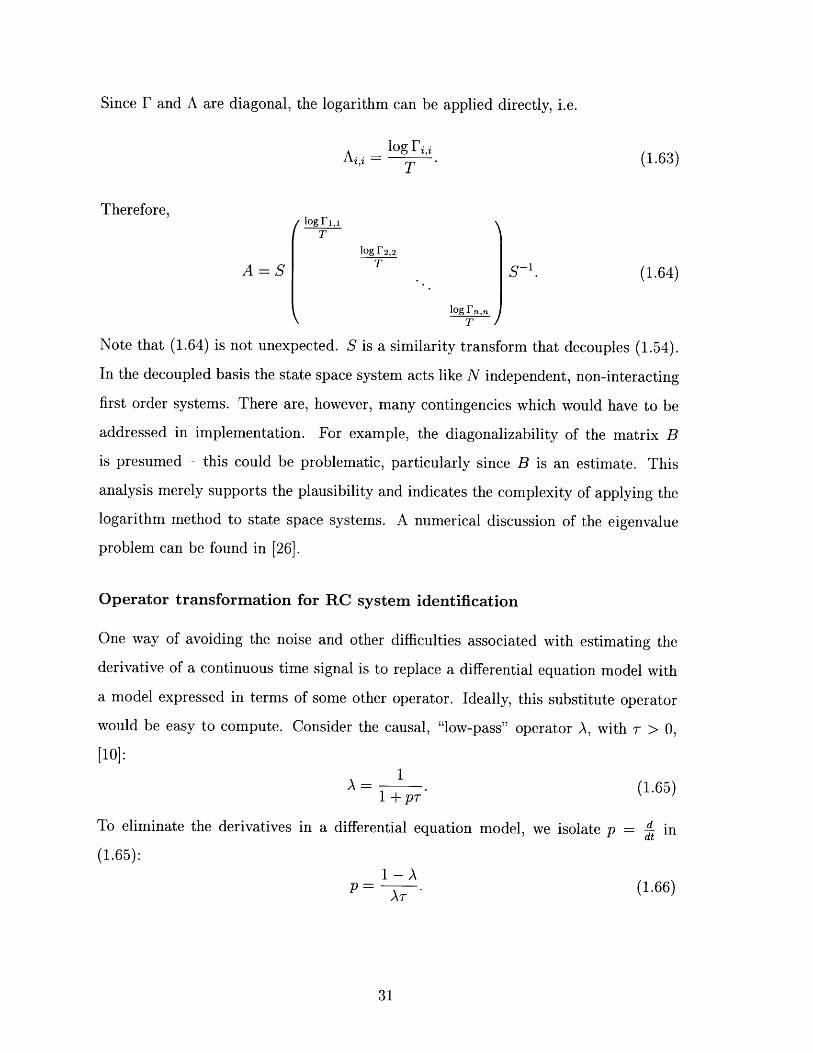
Since F and A are diagonal, the logarithm can be applied directly, i.e.
Ai, log F (1.63)
Therefore,log Fl,
T
log F 2 ,2
A = S T S - 1. (1.64)
log Fn,n
Note that (1.64) is not unexpected. S is a similarity transform that decouples (1.54).
In the decoupled basis the state space system acts like N independent, non-interacting
first order systems. There are, however, many contingencies which would have to be
addressed in implementation. For example, the diagonalizability of the matrix B
is presumed - this could be problematic, particularly since B is an estimate. This
analysis merely supports the plausibility and indicates the complexity of applying the
logarithm method to state space systems. A numerical discussion of the eigenvalue
problem can be found in [26].
Operator transformation for RC system identification
One way of avoiding the noise and other difficulties associated with estimating the
derivative of a continuous time signal is to replace a differential equation model with
a model expressed in terms of some other operator. Ideally, this substitute operator
would be easy to compute. Consider the causal, "low-pass" operator A, with 7 > 0,
[10]:S= 1 (1.65)
1 + p7
To eliminate the derivatives in a differential equation model, we isolate p = in
(1.65):
P - AT (1.66)

Substituting p in the RC system relation
1(R + ;)i(t) = v(t) (1.67)
yields, with some manipulation,
(RC(1 - A) + AT)i(t) = C(1 - A)v(t). (1.68)
A set of normal equations in this new operator can be trivially derived.
/ (1 - A)i[1] Ari[l] (1 - A)v[1]
(1 - A)i[2] ATi[2] R (1 - A)v[2]=1 (1.69)
(1 - A)i[N] ATi[N] (1 - A)v[N]
It should be noted that transformation of the differential equation model to a model
expressed in terms of the A operator does not eliminate the truncation problem asso-
ciated with finite difference approximations to the derivative. The action of A on the
observed quantities must be computed, which requires a finite difference scheme of
some kind. Even if A is computed by the FFT, the various methods of mapping the
continuous time transfer function to a discrete time transfer function are equivalent
to various approximations of the derivative by finite difference methods. For example,
creating a discrete time A by application of the bilinear transform and applying this
discrete time A via the FFT is equivalent to integrating using the trapezoidal rule3 .
There is an advantage, however. The derivative that must be approximated when
applying A is the derivative of the output of the operator, as opposed to the derivative
of the noisy observations. In effect, the sensitivity of the terms involving A to the
approximation involved in computing the derivative can be determined by selection
of 7. Also, it is often possible to arrange the system identification problem so that
3The equivalence of the integration methods and continuous to discrete time transforms is truein an analytical sense. However, the properties of error propagation and the ease with which initialconditions can be constrained are quite different.

the regression matrix consists only of filtered observations and the right hand side
contains all the "noisy" unfiltered observations. Under these conditions, it might be
argued that the regressors would be substantially uncorrelated to the right hand side,
producing unbiased estimates.
1.5.2 Computation of A
The A operator makes the continuous time identification problem relatively straight-
forward. The penalty for simple analysis of the transformed system is the computation
of A.
One attractive possibility for computing A is the "hybrid" scheme suggested in
[10]. Rolf observes that for signals that can be represented by linear combinations
of exponentials est, the A operator (1.65) is precisely the transfer function of an RC
circuitVoLt(s) 1S) (1.70)Vi.(s) RCs + 1
Assuming that the continuous time analog waveforms were available, the response of
a precisely calibrated RC circuit to these waveforms could be sampled. The typical
situation, however, is that only the sampled waveforms are available.
In standard references, e.g. [18], techniques are given for implementing IIR filters
like A. The main step is to select a mapping from continuous to discrete time. This
mapping can be specified in the time domain via a finite difference approximation for
the continuous time derivative like
dx x[k + 1] - x[k]-- T (1.71)dt T
or in the frequency domain via a mapping of continuous time frequencies Q to discrete
time frequencies w, i.e.
w = TQ. (1.72)
Alternatively, one can select a mapping that is based not on a transformation of the
model but rather on some aspect of its response. For example, define a discrete time

transfer function such that the response of the filter to some important signal (like a
step) is conserved.
The mapping used to translate the continuous time filter to a discrete time system
suggests the method used to actually apply the discrete time filter to the data. The
filter transformed with the time-domain mapping (1.71) is a difference equation that
can be iterated, while the filter resulting from (1.72) is most conveniently implemen-
ted using the DFT. In the particular case of the A operator, a reasonably accurate
implementation via the DFT requires more operations and storage than the difference
equation approach. The module lambda. cc in Appendix F implements the lambda
operator using a variable step size equivalent of the finite difference equation.
1.6 Summary
This chapter presents mathematical techniques for the solution of some least-squares
problems often encountered in system identification. This mathematical background
is essential to Chapters 3 and 4. The principle tools reviewed in this chapter include
solution of
* the over-determined linear least squares problem
* the over-determined non-linear least squares problem
* under-determined or badly conditioned problem via SVD
and application to discrete and continuous time system identification problems. A
broad range of system identification problems are susceptible to the techniques of this
chapter, as illustrated by the example of power quality prediction given in Appendix
A. Note that all the mathematical results of this chapter could be expressed in the
form of a minimization of a loss function over the parameter space. For reasons of
computational simplicity, however, explicit minimization of the loss function using
numerical techniques is generally avoided if possible.

Chapter 2
Induction Motor Model
The three phase induction motor model introduced in this chapter is the lumped
parameter model given in [11]. Transformations to an arbitrary, rotating frame are
introduced to interpret the induction motor model. The model is expressed in the
synchronously rotating "dq" frame. Finally, simulation of the induction motor is
considered, and it is seen that simulation is most efficiently accomplished using flux
linkages as state variables rather than currents.
2.1 Arbitrary reference frame transformations
The stator windings in an induction motor are arranged so that applied three phase
currents form a rotating magnetic field. This rotating field induces currents in the
rotor, which usually rotates at a lesser angular velocity. The analysis of machinery of
this sort, where there are rotating fields, structures and circuits, is greatly simplified by
the introduction of a transform that can take sets of variables from the fixed laboratory
frame to an arbitrary rotating frame. Transformations of this type are sometimes
called Parks transformations [11]. The transformation to an arbitrary reference frame
at angle /(t) iscos,3 cos(/3- ) cos( 3 + ±)
K =2 sinp3 sin( - ) sin(3 + ) . (2.1)3 3 3
1 1 12 2 2

The inverse transformation is
cos /3 sin / 1
K- cos( - ) sin(3 - ) 1 . (2.2)
cos(0 + -) sin(3 + ') 1
Note that the transform and its inverse are time dependent through '3(t). A particular
and important example is the transformation to the synchronously rotating frame.
Here
3= t (2.3)
where w is the base electrical frequency. Typically, w = 27r60 rad/s. Equation (2.1)
taken with (2.3) define a transformation to a frame that rotates synchronously with
three phase sources in the laboratory frame. For example, the lab frame three phase
voltage source given by
Scos(wt)Vabc = V0 cos(wt - ) u(t) (2.4)
cos(wt + )3
is, in the synchronously rotating frame,
Vdqo = Vo 0 u(t) (2.5)0)
according to the transformation
VdqO = KVabc. (2.6)
This is an important simplification of the drive typically applied to an induction motor.
The synchronously rotating frame is often referred to as the "dq" frame. Note that
under balanced conditions, where
ia + ib + Zc = 0 (2.7)

, L, L, rr iZqs s _ + 7 qr
+ WAd, (W -Wr)Adr +
Vqs M Vqr
-r Lo L. r,
Figure 2-1: Induction motor circuit model.
and
Va + vb + V' = 0 (2.8)
only the currents iq and id (vq and Vd) need be specified. In the following work,
balanced conditions are assumed. Other important frames include the laboratory
frame, where / is constant, and the frame fixed in the rotor, where
/3(t) = Wr (T) dT. (2.9)
Codes to calculate the arbitrary reference frame transformations, including codes to
translate data in files, can be found in Appendix G.
2.2 Model of Induction Motor (After Krause)
The formulation of the induction motor used here is the same as is used by Krause.
A three-phase, balanced machine is assumed, i.e., (2.7) and (2.8) hold. Figure 2-1
(after Krause, Figure 4.5-1) shows the lumped-parameter model used. The variables
indicated are in the synchronously rotating dq frame. Since the T network of the rotor
and stator leakage inductances L and the magnetizing inductance M form a cut set,

no attempt is made to determine rotor and stator leakages independently. Rather, Lr
is presumed equal to Ls. Also, in the equations that follow, the inductances appear as
impedances at the base electrical frequency of 60 Hz (377 rad/s). For example,
Xm = wM = 1207 -M. (2.10)
The equations that encapsulate the lumped parameter model above are given in terms
of the dq currents and voltages in the following matrix form
rs + Xrr p Xrr Xm P Xm i vw w qs qs
-Xrr r s +XrE -Xm Xm [dsJ V d (2.11)Xm P SX Tm rr + Xrr p
SXrr i, vqr
-sXm X -sX, r + X ir
In (2.11) Xrr = Xm + X1 and p is the operator -. It should be noted that while the
stator currents can be associated with the physical currents in the wires coming out
of a motor, the rotor currents are not as easy to localize. The rotor currents in the
model above are expressed in the synchronously rotating frame, which is not the same
frame as the rotor itself. Furthermore, it is often impossible to make connections of
any kind to the "rotor circuits." This is because the rotor moves and because the
conducting material is often cast aluminum, not individual wires.
The mechanical part of the induction motor equations involve the reaction of the
rotor and mechanical load to the electrical torque induced by the currents above. The
rotation of the rotor enters the electrical dynamics through the slip s in (2.11). The
currents affect the mechanical system through the torque of electric origin, which is
given in [11] as3P
Te = 2 2 M(iqidr - idsiqr). (2.12)
Here, P is the number of poles, M is the magnetizing inductance (not Xm), and the
rotor currents are as reflected to the stator. From basic mechanics, the action of a
torque 7 is to produce an angular acceleration •. The slip, which enters directly into

the above equations, is a normalized measure of the rotor's angular velocity wr.
S= s - Wr (2.13)
Here w, is the synchronous angular frequency, which corresponds to the rotational
frequency of the MMF wave induced by the stator.
Since the only interaction between the electrical system and the mechanical system
is through the slip s, it is advantageous to "recast" the mechanical parameters. The
reaction torque of a moment of inertia J and a friction B is
Tm = J - Bw. (2.14)dt
Sinceds= 1 dWr (2.15)dt ws dt'
it follows that for an induction machine loaded by an inertia and damping only,
dsdt -= 7(idsiqr - iqsidr) + 3(1 - S), (2.16)
where 7 and 3 absorb the inertia and other parameters from equations (2.12) to (2.14).
In particular, note that if the slip is used as a mechanical state variable, the number
of poles can be discarded.
Clearly, it is necessary to limit the complexity of the mechanical load model for
identification purposes. Otherwise, one could imagine a contrived mechanical load that
could create an almost arbitrary signal at the electrical terminals. For the purposes
of this thesis, the electro-mechanical interaction will be limited to (2.16).

2.3 Induction Machine Equations in Complex Vari-
ables
The symmetry in the induction machine equations can be exploited to obtain an
expression equivalent to but more compact than (2.11) using complex variables. This
is accomplished with the following definitions:
is = iqs + jids (2.17)
ir = iqr idr (2.18)
Vs = Vqs + jvds (2.19)
r = qr + jVdr (2.20)
where j = .-1.
The induction motor model (2.11) can then be rewritten as
vs r, + (Xm + Xi)( - j) Xm (P - j) isv, (Xm) ( - sj) r, + (Xm + X1)( - s j)) ir
The economization of notation achieved with complex variables is extremely helpful.
In the routines in Chapter 4, the currents are actually stored as complex pairs because
much of the calculation takes advantage of the complex fast Fourier transform.
2.4 Simulation of Induction Motor Model
An expression providing the derivative of the state as a function of the state and inputs
is necessary to simulate the induction motor. Direct use of (2.11) or (2.21) is not very
efficient because a matrix must be inverted at each time step to find the derivatives.
The matrix inversion can be avoided by using a different set of state variables. Define
the stator and rotor flux linkages per second as
I, = (XI + Xm)is + Xmij (2.22)

fr = (XI + Xm)ir + Xmis.
Using the new state variables I, and Tr the induction motor model can be expressed
in complex form as
vs = rai. + (P- -j)A s (2.24)
Vr = Trir + (P - sj)r. (2.25)
Note that the required derivative appears in (2.25) in a simple way. However, it is
necessary to find is and ir at each step from the evolved states TI and r-. In practice,
simulations of the induction motor using currents as state variables and flux linkages
per second as state variables were found to yield identical results. The simulations
using flux linkages were somewhat faster, as expected.
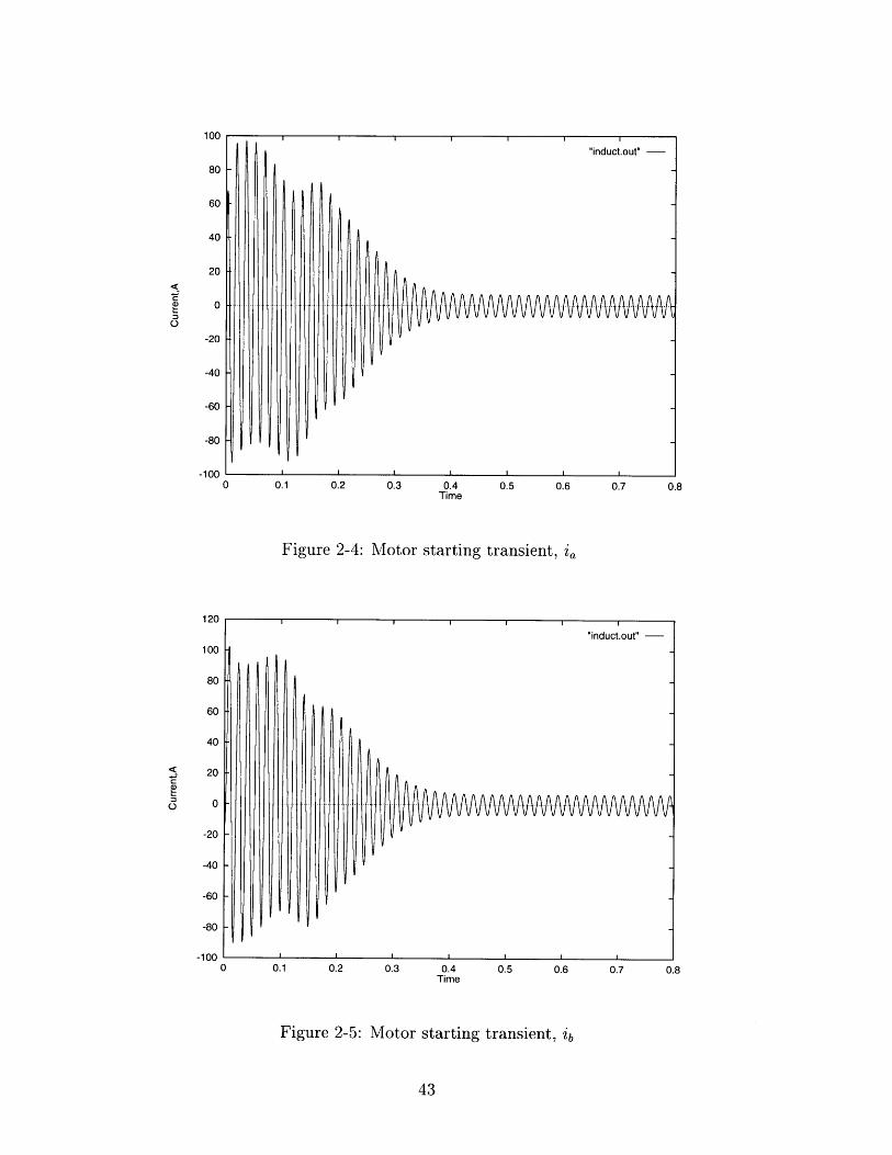
Using the parameters Xm = 26.13Q, Xi = .754Q, rr = .816Q, rs = .435Q and an
inertial load J = .089kg m2 with an excitation of 220 V line to line, the results in
Figures 2-2 through 2-7 were obtained by simulating (2.11). The parameters above
describe a 3 hp rated motor and can be found in [11].
The simulation code, listed in Appendix C, is a fifth order Runge Kutta method
with monitoring of the local truncation error using the fourth order embedded method,
as described in [19]. Local truncation error estimates are used to control the step-size
and bound the errors. This code is substantially derived from Numerical Recipes in
C, although adopted for use with the C++ matrix and vector handling routines used
for this work. Appendix B contains a similar, general purpose simulation code written
in C.
(2.23)

0 0.1 0.2 0.3 0.4 0.5 0.6 0.7 0.8Time, s
Figure 2-2: Motor starting transient, iq,
0 0.1 0.2 0.3 0.4 0.5 0.6 0.7 0.8Time, s
Figure 2-3: Motor starting transient, ids
0 0.1 0.2 0.3 0.4 0.5 0.6 0.7 0.8Time
Figure 2-4: Motor starting transient, i,
-20
-40
-60
-80
-1000 0.1 0.2 0.3 0.4 0.5 0.6 0.7 0.8
Time
Figure 2-5: Motor starting transient, ib
-20
-40
-60
-80
-100

0 0.1 0.2 0.3 0.4 0.5 0.6 0.7 0.8Time
Figure 2-6: Motor starting transient, ic
0 0.1 0.2 0.3 0.4Time, s
0.5 0.6 0.7 0.8
Figure 2-7: Motor starting transient, s
80
60
40
20
0
-20
-40
-60
-80
-100
-120-120

Chapter 3
Extrapolative System Identification
The extrapolative method developed here is motivated by the idea of quickly "eye-
balling" data to obtain reasonably accurate parameter estimates. The parameter es-
timates obtained using this method are not likely to be least-squares solutions, but
might be sufficiently accurate for some applications. In situations where a specific error
criteria such as least squares must be minimized by an iterative routine, the methods
presented here could dramatically increase computational efficiency by supplying a
good initial guess.
The philosophy of the method is to decompose a transient described by a com-
plicated model into smaller domains described by simple, easy to identify models.
The desired parameters are obtained using standard system identification techniques
for these simple models in their respective regions of validity. This situation is illus-
trated in Figure 3-1. The trajectory ( is a transient in phase-space. The trajectory
is entirely contained in a domain for which the full model M is valid. Instead of
attempting to perform system identification given the complicated model M, regions
are identified where the trajectory intersects the domains of simpler models 1 k that
are easy to identify. The simpler models uk are then identified using the portions of
the trajectory for which they are valid. The simple models constrain a subspace of
the parameters of the entire model M, and the combined results of the identification
of the simple models constrain the entire parameter space of M.
As stated thus far, the technique is impractical. This is because for conveniently

Figure 3-1: Phase space illustration of model decomposition.
simple 1Pk, the domains of validity are likely to be vanishingly small. Thus the system
identification of the individual simple models will be constrained to a few data points,
and the results will be extremely sensitive to any noise. To reduce the effects of
noise, it is necessary to identify the simple models over a window. However, the
non-zero width of the window may prevent identification of the model close to its
region of validity. For example, a model valid at the beginning of a set of data cannot
identified over a window centered at t = 0, because there is no data for t less than
zero. The observation that makes the extrapolative method practical is that the region
of support for identifying a model can be extended beyond the neighborhood where the
model is valid. The proviso is that the "model error" outside of the region of validity
be reasonably well behaved. This is illustrated qualitatively in Figure 3-2. In Figure
3-2, the tangent line is proposed as a simple model of a circle valid around the area of
intersection. The dashed line shows the hypothetical estimate of a tangent line based
only on the "noisy" points of the circle around the area of intersection. Although the
dashed line and the solid line are nearly indistinguishable near the point of intersection,
112

+
Figure 3-2: Tangent line model of a circle.
Figure 3-3: Parameterization in the neighborhood of pk•
it is clear from looking at the entire circle that the solid line is a better "fit." Figure
3-2 illustrates directly that a very simple model, valid only for a small region, may be
supported by data in regions where the model is invalid. This is the observation on
which the extrapolative method is based.
To extend the region of support for the simple model beyond its region of validity
in a formal way, it is useful to introduce a parameter 7 as indicated in Figure 3-3.
Then define Tk such that Ik -k M as - -+ Tk, as shown.
Then, the model Pk can be applied to the data to obtain estimates of the parameters
for a sequence of windows 7l, Y2, eti. tending towards Tk. A series of parameter
estimates (-y) will be found. Of course, since the model Pk may not even be close for
some 7, there will be a bias (-y) associated with the estimates (7y). Generally,
X(-) = x(Tk) + fl(7) (3.1)
r
r
rr
r
r
r

X(y)
te
Tk
Figure 3-4: Extrapolation to an unbiased estimated.
where (~y) -+ 0 as -y -+ Tk. The assumption is that not only will 0l(7) tend to zero,
it will also tend to zero in a well-behaved manner. In this case well-behaved means
that a appropriate class of extrapolation functions can be identified a priori. Fitting
the x(y) with a suitable set of functions, we can extrapolate or interpolate to x(Tk)
as shown in Figure 3-4 1. This general idea, i.e. using an extrapolative method to
evaluate some limit of a function, is called Richardson's deferred approach to the limit
[19]. The method is often used in high precision numerical integration routines where
either the limit as the step size goes to zero or the limit as the order of the method goes
to infinity is of interest. The success of the scheme depicted in Figure 3-4 depends on
three conditions. First, the biased estimates must be obtained over windows that are
sufficiently long that the bias l(7y) is a function of model mismatch and not a reflection
of noise. Second, the simplified models Pk must be chosen so that ly(7) is well behaved
approaching Tk. These two conditions are dependent on the model and data at hand.
A third condition is that a suitable class of interpolating and extrapolating functions
must be used to find the unbiased estimates.
1One method of handling colored noise in system identification problems is to add free parametersto "fit the noise" until the residuals are white. The assumption is that the colored noise is filteredwhite noise, and that the filter has some reasonable form. This is analogous to the extrapolativemethod, where we "fit the bias" assuming that the bias is reasonably behaved.
I

3.1 Rational function extrapolation
The class of rational functions has an uncanny ability to approximate well-behaved
functions. This property can be understood rather simply. The general rational func-
tion takes the form of a ratio of polynomials,
R(x) = N(x) (3.2)D(x)
By performing a partial fraction expansion and assuming no repeated roots in D(x),
R(x) = N aix + bi (3.3)i=1 cix - di"
Note that R(x) is a superposition; its general properties can be understood by exam-
ination of the individual bi-linear terms in the sum. Each term is an analytic (except
at the pole) mapping of (0, 1, oc) ý- (x1, x2, 3). For example, if
ax + br(x) = ax + b (3.4)
cx - d
then
br(0) = d (3.5)
a+br(1) = (3.6)
c-d
r(oo) a -(3.7)
If a single term describes a function of time, for instance, the function can be given
particular values at 0, some arbitrary time t, and the limit of the function as t -+ oo
is perfectly well defined. The rational function expansion is particularly suitable for
capturing overall behavior of functions. For example, the term
f(t) (e- 1t+ (3.8)(e - 1)t + 1

1.2
1
0.8
0.6
0.4
0.2
00 2 4 6 8 10
t
Figure 3-5: Truncated Taylor series and rational approximations to e- t .
approximates f(t) = e- t reasonably well between the support points 0 and 1 and has
the same limit as t -4 oc. In contrast, a finite order polynomial approximation for e- t
based on the Taylor series expansion
t t2 3 (-tne- = 1-t+ +·+ +.t (3.9)2! 3! n!
is guaranteed to be unbounded as t - oc; adding more terms doesn't help. This is
illustrated in Figure 3-5. In Figure 3-5, a fourth order truncated Taylor series and first
order rational function approximations to e-t are compared to the actual function. The
consequence of the bi-linear term is that a rational function interpolator or extrapolator
is likely to have reasonable properties approximating functions with common features;
poles, well defined limits, etc. The drawback is that computation of the coefficients of
a rational function interpolator given data is not trivial [19], [26]. Fortunately, because
of the importance of rational function expansions in Richardson extrapolation and in
established methods like Romberg integration and the Bulirsch-Stoer method, methods

are readily available [19].
3.2 RC Example
The extrapolative technique 2 is easily applied to the RC system identification example
of Chapter 1. The RC response to a voltage step v(t) = u(t) is
i(t) = Re T R. (3.10)
In the neighborhood of t = 0,t t
Re R 1- (3.11)RC
by truncation of the Taylor series. Therefore, a "low-time" model is
1 ti(t) (1 - RC ) . (3.12)
Equation (3.12) can be used as a model in a suitable domain to find R and C.
Using the extrapolative technique, however, the model (3.12) is applied for a sequence
of -y converging on 0. This is shown in Figure 3-6, where a series of possible "fits"
of the linear, low time model are applied to the current transient i(t) for R = 1I
and C = .3F. In Figure 3-6 the parameter of each low-time fit is 7 = t. In practice
the fits in Figure 3-6 would be evaluated over windows to reduce the effects of noise.
The low-time model fit at y = 1, for example, might be based on data in a window
extending from t = 0 to t = 2.
The low-time model fits shown in Figure 3-6 are interpreted as a sequence of
biased estimates for R and C; the next step is to extrapolate the estimates to zero
bias. Estimates at zero bias are found by assuming that a "reasonable curve", like a
rational function, will capture the behavior of the bias in the parameter estimates as
a function of the parameter y. In this case, since the model is a "low-time" model,
2In the extrapolative method, the estimates of the system parameters (i.e. R and C) are themselvesparameterized (by y). To avoid confusion, in this example "parameter" refers to -y and "estimates"refers to R and C.

0.6
i(t)
0.4
0.2
00 2 4 6 8 10
Figure 3-6: A sequence of fits of the "low-time" model to an RC transient.
the sequence of estimates are extrapolated to -y = 0. The extrapolation process for
the estimates R? and C is depicted in Figure 3-7. In Figure 3-7 rational function
approximations of R(-7) and C(y) based on the estimates at 7y = 1, 2, 4 are shown.
The rational function approximations are used to extrapolate the values of R(-y = 0)
and C(-y = 0), which should be unbiased estimates of the system parameters R = 1
and C = .3. For comparison, continuous plots of
() -) = (3.13)
and-1
C(y) = (3.14)R (7)i'(7)are also shown. Theoretically, R and C would result from the noiseless identification
of the low-time model over differentially small windows centered on 7. These plots are
shown to illustrate how the rational function extrapolator approximates the model error

2 4 6 8
2 4 6 8
Figure 3-7: Extrapolation of the unbiased- = 1,2,4.
estimates R(0) and C(0) from estimates at
2
0
0
0.35
0.3
0.25
0.2
0.15
0.1
0.05
0
0

bias (•,y). In practice the estimates at 7 = 1, 2, 4 would be obtained from measured
data and the plots of R and C would be unavailable. A slight error is evident in the
extrapolation to R(O) in Figure 3-7. This error arises because the rational function
extrapolation, given the three support points shown, does not precisely model the
bias. The extrapolative method is approximate. Nevertheless, Figure 3-7 shows that a
rational function expansion of model error bias allows a simple model (equation 3.12)
to be used for the identification of a more complicated model given data for which the
simple model is invalid.
3.3 Simplified induction motor models
To apply the extrapolative system identification technique, one need only find simple
models of the more complicated system in question. For the RC circuit, and for any
system with a known response of the form eAt, a simplified model can be extracted
from the Taylor series. A simplified model that takes advantage of the Taylor series
for eA t avoids the continuous time identification issues discussed in Chapter 1. In the
case of the induction motor, we would like to avoid the complication that the rotor
currents in the standard model (2.21) are not measured. This is accomplished by
developing simple models for the induction motor in the neighborhood of t = 0, when
the rotor is inertially confined, and t = oc, when the motor and load are in steady
state.
An implementation of the high and low slip models below applied using the extra-
polative identification procedure can be found in Appendix D.
3.3.1 Model for high slip
Under the condition s = 1, which persists at t = 0 due to inertial confinement of the
rotor,
ir = -is. (3.15)

The induction motor may be thought of as a transformer with a shorted secondary in
this state. Substituting (3.15) into the complex induction motor model (2.21) yields
vs = (rs + Tr)is + 2X,( p - j)is. (3.16)w
This is the simplified induction motor model, valid as t -- 0. In the first instants
of induction motor operation, therefore, two degrees of freedom are eliminated. In
particular, the parameter X, and the sum of the parameters r, and rr can be found.
Furthermore, (3.16) is valid for any realistic mechanical load.
3.3.2 Model for low slip
For an inertial load, the slip goes to zero in the steady state. In the limit of low slip,
there is no torque, hence ir = 0. Again substituting into (2.21),
vs = rsis + (X 1 + Xm)(( - j)is. (3.17)
The portion of the transient that approaches steady state therefore eliminates two
additional degrees of freedom. Combined with the data given by the in-rush current,
the four electrical parameters of the induction motor are completely specified.
Mechanical situations more complicated than a simple inertia are generally of in-
terest. These problems can be solved by applying the extrapolative method to the
"steady state" model in [11], provided that the mechanical excitation allows the con-
ditiondsd-t - 0. (3.18)
In other words, the mechanical system must have a constant or slowly varying steady
state relative to the electrical time constants. Note that this condition may be easier or
more difficult to satisfy depending on the rating and design of the motor. If the steady
state mechanical situation allows relatively error free use of the steady state induction
motor model it can be used for identification of the remaining mechanical and electrical
parameters in the same fashion as (3.17). System identification of induction motors

using the simple steady state model is discussed by [5] and [29].
3.4 Summary
The extrapolative estimation procedure outlined here obtains quick estimates of the
parameters of complicated models by applying standard system identification tech-
niques to reduced models in the temporal domains for which the reduced models are
valid. Rational function extrapolation is critical both because it allows the region of
support of the estimates to include more data and because it allows the use of models
that are valid only "in the limit." To apply the method, one need only derive reduced
order models.
The prime advantage of the extrapolative method is that it is fast and easy to
implement. For example, in the case of the induction motor, the complexity of the full
transient model is irrelevant; one need only consider the simple "blocked rotor" and
"steady state" models. The extrapolative method implemented with rational functions
is especially attractive because model simplifications that are true "in the limit" can be
exploited. For example, in the case of the induction motor the approximation if = -is
is used even though this is true only as t -+ 0.

Chapter 4
Modified Least Squares
In this chapter, a conventional approach to finding the induction motor parameters
is developed. The basic idea is to formulate the system identification problem as a
minimization and to solve that minimization problem. It is seen that finding a loss
function is rather simple, but finding a loss function that is quickly minimized is not.
The notation of the complex induction motor model (2.21) is used throughout.
The problem of finding the induction motor parameters can be stated mathemat-
ically in a simple way. Since the excitation v, and the stator currents iZ are known or
measured, an estimate of the parameters is given by a minimization of the form
a = arg min V(x, iZ, v,). (4.1)
One candidate for the loss function V(x, i5 , v,) is to set i' to the results of a simulation
using the parameters x and the excitation v,. Then the loss function is the squared
error between the observed and simulated currents, i.e.
V(x, is, v) = (is - i~(vs, x))T(is - i'(v 5 , x)). (4.2)
Theoretically (4.2) could be minimized and the resulting x would be the least-squares
parameter solution. Unfortunately, the necessarily iterative procedure to minimize
(4.2) requires an expensive simulation for every step. While implementation is simple,

assuming that a sufficiently sophisticated minimization routine exists, the time re-
quired makes this algorithm unacceptable. The challenge is to design a loss function
that is computationally easy to minimize.
4.1 Eliminating the rotor currents
Incorporating the simulator at every stage of the minimization is a slow way of avoiding
the difficulty that the rotor currents ir are not measured. If the rotor currents were
measured, then techniques of Chapter 1 could be used without modification- i.e.
form a regression matrix based on the model and solve for the parameters. Another
strategy for dealing with the unmeasured rotor currents is to algebraically eliminate
those quantities from the model. The transformed model, expressed only in terms of
measured or known quantities, could then be used to find the desired parameters. For
example, if
c d) X2 = r2 (4.3)
and x 2 is not measured, then if b (in general, an operator) is invertible,
cxl + db-'(ri - axl) = r2 . (4.4)
Equation 4.4 has the desired property of containing only x1 , and the standard tech-
niques from Chapter 1 could be applied to finding the parameters in the operators a
through d. If b is not invertible, x2 can still be eliminated. Applying b and d to (4.3)
yields
bcxl + bdx 2 = brl (4.5)
daxl + dbx 2 = dr 2. (4.6)
If the commutator (Lie bracket) [b, d] = bd- db is equal to zero, then the term bdx2 can
be isolated in one equation and substituted in the other, eliminating x2 . If [b, d] = 0,

then
daxz + brl - bcxl = dr2. (4.7)
The complex induction motor model
VS Ts + (Xm + X) (P- j) Xm ( - ) i (4.8)r (Xm)( - sj) r + (Xm + Xi)( - sj) ( r
has the same form as (4.3). Eliminating ir by inverting one of the operators acting on ir
does not seem promising. Both operators acting on i~ have a zero; their corresponding
inverses have a pole which could introduce internal stability issues. The operators
acting on ir also have a non-zero commutator due to the time variation of s. To
eliminate ir, a choice must be made between errors due to the pole in the inverses, or
errors due to the non-zero commutator.
4.2 Rotor current observer
Since the rotor currents cannot be eliminated algebraically, the next best thing is to
estimate the currents and attempt to confine the resulting errors. The most stable
method found, from the point of view of numerical errors, was to use the quantity T,
to find i,. In particular, (2.24) can be rewritten to obtain,
Ts = W (v - rTsis) (4.9)p - w3
which can be used to estimate TI from the measured quantities v, and is. Recall that
the base frequency w = 27r60. Using the definition of Ts,
Ts = Xm(ir + is) + Xli s (4.10)
ir can be estimated1
S= = (JFS - Xmis - Xtis). (4.11)Xrn

To the extent that (4.9) can be computed accurately, then, ir is expressed in terms
of the parameters and the observations is and v,. In Appendix E, equation (4.9)
is implemented using the FFT. Although the partial derivatives of this rotor current
observer are of interest, considerable effort can be saved by postponing the calculation
of partials until the error introduced by the pole in (4.9) is handled.
4.3 The loss function
Having used half the induction motor model to create an observer for the rotor cur-
rents, only the second half
Vr = Xm(p - sj)is + (rr + (Xm + X)(P - sj))i (4.12)
remains for use in the loss function. Note that under the assumed conditions of single
excitation, Vr = 0. However, if the parameters are incorrect or if ir is not equal to the
unmeasurable ir, Equation (4.12) will have some error e,
= Xm( W sj)is + (rr + (Xm + XI)( - sj))ir. (4.13)
The error e will be a combination of the errors due to the observer pole at w and the
errors due to incorrect parameter values 1. However, the errors due to the observer pole
will be in a small neighborhood in the frequency domain around the pole frequency
w. Although the errors due to the observer pole are modulated by the time variation
in the slip, the slip is relatively close to DC (given reasonable mechanical loads) in
comparison to the observer pole frequency. The errors due to parameter mismatch
will be at lower frequencies. For example, if Tr is off by 6 the error f will be a "copy"
of the relatively low-pass rotor current, i.e. C = 64r. The situation in the frequency
domain is depicted schematically in Figure 4-1. The indicated solution is to minimize
fTe in the frequency domain at those frequencies where the artifact introduced by the
1Note that according the definition of the error in (4.13), the estimated parameters will not be"least-square parameters" in terms of the observations is.

Parameters
Figure 4-1: Sources of error in the frequency domain.
lel
f -*8 I<- W
Figure 4-2: Errors are minimized in a selected band.
observer pole has no effect. Note that minimization can be performed in the frequency
domain with the same effect as minimization in the time domain. This is guaranteed
by Parseval's relation [24] which for a discrete time signal x[n] and its DFT X[k] is
1SIIX12 = |lX112.N (4.14)
That is, anything that forces the error to zero in the frequency domain also forces
the error to zero in the time domain. Furthermore, if the disturbances in the time
domain are white, the power spectral density is uniform. The advantage of using the
frequency domain is that the minimization can be applied selectively to the errors that
are due to parameter mismatch, ignoring the observer pole artifacts, as indicated in
Figure 4-2.
61
a,
Observer pole
--->i
i

0.9
0.8
0.7
0.6
0.5
0.4
0.3
0.2
0.1
0
-0.10 200 400 600 800 1000
Figure 4-3: Blackman window.
4.3.1 Spectral Leakage
As a consequence of the finite-length of practical data sets, the error introduced by
the observer pole spreads into nearby frequencies. This phenomenon is called spectral
leakage [18], [10]. In the minimization problem, the difficulty is that spurious data
due to the observer pole may "leak" to the frequency range where the error is being
minimized. The effect of spectral leakage is shown in Figure 4-2 where the observer
pole is "smeared." A practical measure for containing this spectral leakage is to
window the time-domain errors e. Various windows are available; any reasonable
function that goes to zero smoothly at two points will do. For this work, a Blackman
window
0.42 - 0.5 cos(2--) + 0.08 cos(n4 ) 0 < n < Mw [n] = (4.15)
0 otherwise
was used [18]. Equation 4.15 is plotted in Figure 4-3 for M = 1024.

4.3.2 Partial Derivatives
Algorithms for minimization typically require the availability of partial derivatives of
the error with respect to the parameters at various values of the independent variable.
If the minimization is performed in the time domain, the desired partials are - for
the parameters xi. The partials in the frequency domain are related via the DFT 1
a ic = ( ). &(4.16)Xi f Xi t
For simplicity the partial derivatives are given here in the time domain, with the
understanding that the partials must be windowed and transformed to minimize the
windowed and transformed loss function.
First, consider the effect of the rotor current observer. Although the estimation of
rotor currents is performed for numerical reasons via the flux linkages, the algebraically
equivalent expression in currents can be used for computation of partial derivatives.
The relevant equation is
vs = rsis + (Xm + X 1)( - j)is + Xm( - j) (4.17)W W
Since the minimization is confined to low frequencies as shown in Figure 4-2, the
approximation
P- 0 (4.18)
is valid. Setting P to zero in (4.17),
vs = rsis - j(Xm + Xi)is - jXrmr. (4.19)
Using the fact that '9 is zero for all parameters x, the partials ' are, in the limit of
low frequencies,
dir is+ r (4.20)OXm Xm

-r - - is (4.21)OX1 Xm
= 0 (4.22)Orr
= -Z (4.23)Or, Xm
Ultimately the partials o for all parameters x are desired. Applying the approximation
(4.18) to (4.13) yields,
E = -SjXmis + rrir - sj(Xm + Xl)ir. (4.24)
Application of the chain rule and appropriate substitutions yields
=- (rr sjX s ar (4.25)
S-sj(zr - iZs) + (rr - sjX) r (4.26)ax, dXI
rr Zr (4.27)
r, (4.28)ar
That the partial derivatives of the error function can be expressed analytically makes
the minimization of the associated loss function susceptible to a broad range of al-
gorithms. The problem as stated is suitable for the Gauss-Newton procedure from
Chapter 1, for example. While Gauss-Newton is attractive for its speed and sim-
plicity, in situations where it is undesirable to repeatedly modify the initial guess to
achieve convergence a more stable algorithm is preferable. The suggested algorithm is
Levenburg-Marquardt, given in [2] and [19]. Minimization of (4.24) given the partial
derivatives in 4.28 using the Levenburg-Marquardt algorithm is implemented in the
files identify.cc and estimate.cc in Appendix E. The file mrqmin.cc is a slightly
modified version of the like-named file from Numerical Recipes [19].

4.4 The mechanical interaction
The proceeding development neglects the mechanical system associated with the in-
duction motor. The partial derivatives of the error function are written assuming
that = 0 for any parameter x, and therefore the equations above are useful for
the case where s(t) is actually measured. Measurement of s(t) is a great advantage,
because it effectively decouples the electrical and mechanical systems. Without s(t)
the parameters of the mechanical system must be identified in addition to electrical
parameters from the electrical transient only. At some point, the complexity of the
combined electrical and mechanical model might exceed the information content of
the electrical transient.
In many cases, it might be possible to work around the limited information con-
tent of the transient. This is because the mechanical system is often simple during
the electrical startup transient. For example, in typical operation of a machine tool
like a lathe or mill, the induction motor is started with only an inertia and windage
load. Then the cutter is applied to the material, introducing a mechanical disturbance
and a substantially more complicated modeling problem. However, it is possible that
during the initial startup transient, the induction motor parameters and the simple
mechanical model could be identified and used in the subsequent operation of the tool
to gather information about the machining process, for instance. Furthermore, if no
slip information were required, this data could be gathered non-intrusively. Identifica-
tion of the induction motor parameters and a relatively simple mechanical load model
is therefore likely to be helpful even in complicated scenarios.
4.4.1 Slip estimation by reparametrization and shooting
The electro-mechanical interaction of the induction motor with an inertial and damping
load is governed by Equation 2.16, reproduced here for convenience
dsdt - Y (idsiqr - iqsidr) + /(1 - S). (4.29)dt

Define a time to when the system enters steady state such that
ds(to) 0 (4.30)dt
and define the steady state slip
so = s(to) (4.31)
also, let the torque estimate
(t) = idsqr - iqsdr. (4.32)
With these definitions, 3 is determined as a function of y:
f = (4.33)1 - so
Substituting into (2.16),
d- (t) + (1- ). (4.34)dt 1 - so
Assuming that so and to are specified, Equation 4.34 is a boundary value problem.
Thus, 3, y and s(t) can be found by a one dimensional shooting method [26]. Ef-
fectively, the parameters so and to have been substituted for the parameters y and 3.
There are many advantages to this reparametrization. Any t in the steady state oper-
ating region of the motor is a suitable to. In practical terms, if the startup transient of
a motor is fully captured, to is simply the last time coordinate in the data set. Also,
it is likely that so is known with reasonable accuracy; the speed at rated load is often
printed on the machine. Even if the steady state slip cannot be determined a priori,
so is a much "friendlier" parameter than either y or 3 because it is dimensionless,
bounded absolutely 2 by 1 and 0, and bounded approximately by the torque estimate
?(to) and the machine rating. Another advantage of introducing so as a parameter is
2 1t is assumed that whether or not the machine is being used a generator is known.

that the slip estimate .(t) is approximately independent of the electrical parameters.
The electrical parameters are involved through Z,, but the overall scaling of the slip
estimate is determined by the "boundary condition" so.
The shooting method for slip estimation is implemented in Appendix E. A hybrid
Newton/bisection shooting algorithm finds a - on each iteration to match the boundary
condition so given the updated rotor current estimates. The Newton method is tried
first, and the bisection method is used if the Newton method fails. The computational
cost of the shooting method is minimal, since the results of the previous iteration are
used as an initial guess. Shooting methods are discussed in [26],[19].
4.4.2 The general case
The general case, with an arbitrary mechanical load, can be addressed by estimating
the slip based on the rotor current observer, the mechanical model and its tentative
parameters. However, with the rotor current observer used here the approach is
problematic. The difficulty is that the rotor current observer pole introduces high
frequency errors in the rotor currents. To predict torque, the rotor currents are
multiplied by the stator currents. If the stator currents have frequency content at
the rotor observer pole frequency, the multiplication produces an image at DC and
at twice the frequency of the rotor observer pole. The high frequency component
tends to have little effect on the slip due to the mechanical filter formed by the inertia
in the mechanical load model; the DC torque component, on the other hand, has a
substantial effect. This is an area that requires further investigation.
4.5 Summary
The induction motor system identification problem is relatively easy to state math-
ematically as a minimization. Given a simulator for a system, a loss function can
be written incorporating the simulator that expresses exactly the intent of the identi-
fication procedure - to find a set of parameters matching the observations in a least
squared sense. The problem is that such a loss function is expensive to evaluate and

LevenburgMarquardtAlgorithm
is
Rotor CurrentObserver
(4.11)
1,ax
is
7 r TorqueEstimator
(4.32)
MechanicalError Function (t) Model
• (4.13)-+ Window * (4.34)FFT -+ Window
Figure 4-4: Schematic diagram of modified least squares method.
difficult to minimize.
In this chapter, a computationally efficient loss function is formulated. First, a
rotor current observer is presented. The estimated rotor currents are used to estimate
torque and also to compute components of the error. The error is minimized using
the Levenburg-Marquardt method, which requires the partial derivatives of the error
with respect to the parameters.
Two methods of dealing with the mechanical system are presented. First, if s(t)
is supplied, the identification of the electrical parameters is decoupled from the mech-
anical interaction. Slip measurements are very valuable if available, because then
the electrical and mechanical identification problems can be treated independently. If
s(t) is not available, and the load is assumed to be inertia and damping only, the
mechanical subsystem can be reformulated using a shooting technique so that the new
parameters are either known a priori or easily estimated. An additional advantage
of the reparametrization is that the approximate slip can be treated as independent
of the electrical parameters. This allows the same partial derivatives to be used for
minimization whether or not the slip is measured.

A block diagram of the entire estimator is shown in Figure 4-4. In Figure 4-4 - is
the estimated vector of parameters, and it is assumed that the slip must be estimated.
The numbers in the diagram indicate the equations associated with each block.

Chapter 5
Results
The induction motor identification methods presented in this thesis were validated
using both simulated and measured data. Tests using simulated data compare the
estimated parameters to the parameters used to create the simulated data. No noise
was added to the simulated data. To evaluate the performance of the methods on
real data, estimated parameters were used to create simulated transients which were
compared to the collected data. Note that validation with simulated data tests the
identification procedure in isolation, where validation with measured data tests both
the motor model and the identification procedure.
5.1 Simulated data
Simulated data were obtained using the simulator discussed in Chapter 2. Figure 5-1
demonstrates the variety in the simulated motor test data. Figure 5-1 is a composite
plot of transient currents iqs and slip curves for several different motors. The motors
are the 3 hp, 50 hp and 500 hp motors used as examples in [11]. Note that the
500 hp transient includes generative operation of the motor, as the slip goes negative
around sample number 3500. The 2250 hp test motor is qualitatively similar to the
500 hp transient, except that the peak current is in the neighborhood of 4000 A. To
preserve the character of the lower power waveforms, the 2250 hp transient is not
shown. Note that the sampling rates for the different transients are not the same; the
data is sampled as used for identification.70
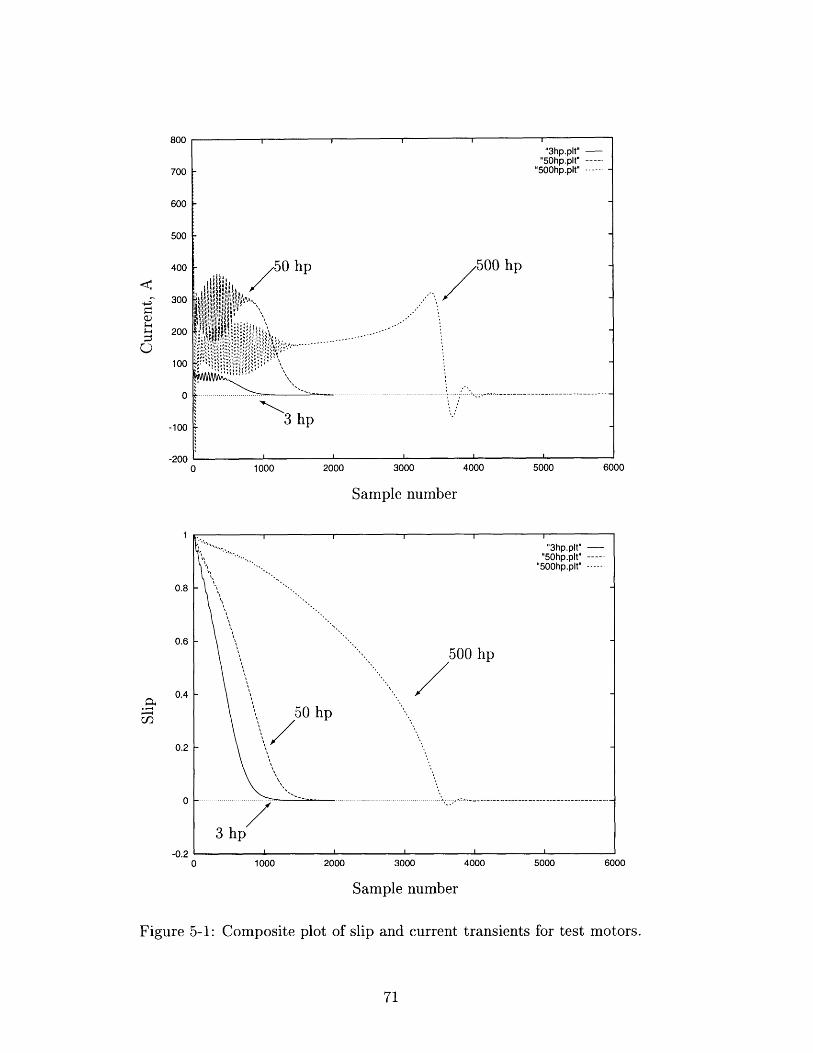
700
600
500
400
300
200
100
0
-100
-900
1
0.8
0.6
0.4
0.2
0
-n 9
0 1000 2000 3000 4000 5000 6000
Sample number
0 1000 2000 3000 4000 5000 6000
Sample number
Figure 5-1: Composite plot of slip and current transients for test motors.

Motor
Xm3 hp XA
220 V r,rs
Xm50 hp X 1460 V rr
rs
Xm500 hp X12300 V r,
rs
Xm2250 hp X12300 V rr
rs
TrueParameters
(Q at 60 Hz)26.13.754.816.435
13.08.302.228.087
54.021.206.187.262
13.04.226.022.029
EstimatedParameters
(Q at 60 Hz)26.144
.739.808.434
13.38.2917.2702.064754.101.205.472.214
13.03.231.034.029
Table 5.1: Extrapolative method estimates, simulated data.
5.1.1 Extrapolative method
Results for the extrapolative method presented in Chapter 3 are shown in Table 5.1.
The column labeled "true parameters" contains the values used by the simulator
to generate a transient. The column labeled "Estimated Parameters" contains the
parameters output by the extrapolative identification program.
Recall that no initial guess is required for the extrapolative method, and that the
method is not iterative.
5.1.2 Modified least-squares method
Table 5.2 shows data obtained using the modified least-squares method presented in
Chapter 4. No particular care was taken in picking initial guesses, although informal
experimentation revealed that the convergence of the method was rather robust. Rig-
orous analysis of the convergence properties of the method is left to future work.

MotorXm
3 hp Xi220 V r,
rs
Xm50 hp X 1460 V rr
rs
Xm500 hp Xi2300 V rr
_rs
TrueParameters
(Q at 60 Hz)26.13.754.816.435
13.08.302.228.087
54.021.206.187.262
InitialGuess
(Q at 60 Hz)24.01.01.00.3
10.00.50.5.1
50.01.0.3.4
Estimated Parameterss(t) given
(Q at 60 Hz)26.19.7496.8130.435813.07.3018.2263.088048.821.207.1843.2672
s(t) unknown(Q at 60 Hz)
26.49.7521.7705.416912.99.2984.1950.084552.221.207.1829.2643
Table 5.2: Modified least-squares method, simulated data
In Table 5.2, "True Parameters" are the parameters used by the simulator to
generate test data. The "initial guess" column lists the parameter guess passed to the
iterative method. Note that the initial guesses in Table 5.2 are uniformly worse than
than the results from the extrapolative method listed in Table 5.1. The modified least-
squares method was run both with a "measured slip" and with a slip estimator, as
discussed in Chapter 4. The slip might be available in some situations; for example,
when characterizing a particular motor for control purposes. The "slip unknown"
column corresponds to the nonintrusive diagnostics scenario, where slip measurement
is not possible.
5.2 Measured Data
Real data was obtained from transient tests on a typical three-phase industrial induc-
tion motor. The test induction motor was connected to a three-phase 208 V line to
line 30 A rated service using a solid state three-phase switch with a programmable
firing angle [15]. Voltage and current data during the startup transient were collected
on a four channel TDS420A digital storage oscilloscope using isolated A6909 voltage

Leyland-Faraday Electric CompanyType: AEEA Model: LFI-3050 Phase: 3
Hp: 5 Volts: 208-230/460Rating: Cont Cycles: 60
AmbTemp: 40 C RPM: 3420-3480Frame: 184 T Service Factor: 1.15Amps: 12/6 Nema Design: B
Table 5.3: Boiler-plate data from test induction motor
and A6303 current probes. Since the firing angle was under computer control, the
experiment was assumed to be repeatable. Hence, the current and voltage measure-
ments were actually made in two successive tests. For synchronization of the two
tests, one channel of voltage information was stored while collecting the three cur-
rents. The oscilloscope was set to trigger from this voltage channel for both current
and voltage measurements. Data collected by the oscilloscope was stored on disk in
Tektronix .WFM format and translated to files suitable for input to the identification
procedures by the BASH script and C programs listed in Appendix G.
The boiler-plate data from the test induction motor is reproduced in Table 5.3. No
mechanical load, except for the rotor inertia and windage, was attached to the motor.
Figure 5-2 shows the current transient and resulting voltage distortion for the
test motor in the dq0 frame. Note that while the maximum-load power rating of the
motor is within the 30 A per phase rating of the three phase service, the motor draws
currents well in excess of 30 A during the startup transient. Also, the assumption of
balanced conditions seems to be violated; both the voltage and current have a "zero"
component, particularly in the high current portion of the transient.
The "spikes" on the voltage plots are associated with the switching of the alternistor
used to control the three phase switch. The currents per phase during the first .2s
exceed the alternistor's steady state rating by about a factor of four.

20
0
-20-U.1 0 0.1 0.2 0.3 0.4 0.5 0.6
Time, seconds
-100-U. I U 0.1 0.2 0.3 0.4 0.5 0.6
Time, seconds
Figure 5-2: Current and voltage measurements in dqO frame, unloaded motor.

5.2.1 Extrapolative method
The extrapolative method was used to analyze the motor transient data in Figure 5-2.
The program elh from Appendix C was used, as shown in the following interaction.
darkstar:/home/sshaw/elh# elh < small.elhElh Version 0.1a I Data from 5 hp induction motorSteve Shaw, 1996125014005000100000.03140004e-05Error Margins show error expected in extrapolation.They are not a reflection of the data quality.X1 = 0.546740, +/- -0.027198Rr+Rs = 0.710156, +/- 0.048885Xss = 39.521109, +/- 0.049014Rs = 7.609524, +/- 1.864681darkstar:/home/sshaw/elh#
The output above seems reasonable except for the value of rs. The error margin
and unrealistically large value for rs indicate that the method had problems identifying
the "low-slip" model. This was expected, because the low-slip model used was for an
inertial load; the real motor's mechanical load includes unmodeled friction from the
fan and bearings. The extrapolative method is intended to provide reasonable initial
guesses for an iterative method, however, and accurate identification of a partial set
of parameters is still valuable information. To confirm that the estimates X 1, rr + rs
and Xss = Xm + X1 determined by the extrapolative method are reasonable requires
comparison of a simulated data set (using those parameters) with the measured data
set. The following parameters were used to generate a simulated data set.
XI = .547Q
Xm = 38.97Q

Rr = .355Q
Rs = .355Q
a= .05Q
Since the extrapolative method estimate of rs was assumed invalid, rs and r, in the
above parameter set are arbitrarily made equal. The mechanical parameter a = .05
was picked so the transient would have approximately the right length. It should
be emphasized that the above parameter set was not completely generated by the
extrapolative method presented. Only three degrees of freedom in the parameter
space were determined by the extrapolative method. Guesses for the remaining two
degrees of freedom are supplied so that an induction motor simulation can be used
to confirm that the estimates that were produced by the extrapolative method are
valid. The simulation should closely match the measured data at the beginning of
the transient, since the extrapolative method was able to identify the high-slip model.
Comparison of the simulated and measured data in the middle of the transient is
not meaningful. At the end of the transient, the steady state should be reasonably
accurate since Xm > rs and the load is light. The simulated and measured data sets
are compared in Figure 5-3.
The insets in Figure 5-3 show the agreement between measured data and simulated
data in the high slip region where the extrapolative method was successful. Note that
the large discrepancy in the comparison of ids is likely due to the voltage distortion of
Vds (see Figure 5-2). The simulations shown in Figure 5-3 do not take the line voltage
distortion into account.
5.2.2 Modified least-squares method
The measured induction motor data was also analyzed with the modified least squares
method presented in Chapter 4. The initial guess (in Q at 60 Hz) was X, = 1.00,
Xm = 45.0, and rr = rs = .5. In addition, the slip so at to = .4s was estimated to
be .005, approximately an order of magnitude below the slip at rated load according

0 0.1 0.2 0.3 0.4 0.5 0.6
Time, seconds
14U
-0.01 0 0.01 0.02 0.03 0.04 0.05
-0.1 0 0.1 0.2 0.3 0.4 0.5 0.6
Time, seconds
Figure 5-3: Comparison of simulated and measured transients.
20
0
-9n-0.1-0.1
40
20
4 A/•I
1 I
I

to the motor rating. The following screen interaction was obtained by running the
program identify from Appendix D. Note that the parameters below are listed in
the order Xm, X 1, rr, rs. The fifth parameter shown is not used, and beta is the
mechanical parameter used to estimate the slip. Chisq is the squared magnitude of
the residual, and i = 6 indicates that the method converged in six iterations.
beta = 0.396901Chisq[6] = 546.911638Alambda[6] = 0.000100
Stopping. i = 6Chisq = 546.911638
parameters:3.847e+016.048e-013.356e-014.767e-013.000e-01covariance matrix:2.8e+00 9.5e-04 -1.3e-04 -4.4e-04 0.0e+009.5e-04 4.5e-06 4.5e-07 -2.6e-07 0.0e+00
-1.3e-04 4.5e-07 1.4e-05 -2.6e-05 0.0e+00-4.4e-04 2.6e-07 -2.6e-05 6.2e-05 0.0e+000.0e+00 0.0e+00 0.0e+00 0.0e+00 0.0e+00
The parameter estimates displayed above compare favorably to the results from
the extrapolative method. In addition to the electrical parameters, the modified least
squares method also generates a slip estimate shown in Figure 5-4, as described in
Chapter 4. Note that the test motor overshoots at t = .2s, according to the predicted
slip curve. Note that the mechanical parameters, although not displayed above, are
easily obtained from the estimated slip curve and electrical parameters.
To validate the estimates generated by the modified least squares method, the
estimated slip shown in Figure 5-4, the distorted voltage waveform from Figure 5-2
and the parameter estimates were input to a simulator in an attempt to reproduce

0.6
0.4
0.2
0
-0.2-0.1 0 0.1 0.2 0.3 0.4 0.5 0.6
Time, seconds
Figure 5-4: Estimated slip, modified least-squares method.
the measured currents. This test not only verifies the accuracy of the parameter
estimates, it also validates the applicability of the induction motor model assumed in
this thesis. It should be noted that while the distorted voltages vqs and vds were used
in the simulation, the imbalance (i.e. vo, in Figure 5-2) was ignored. The measured
and simulated currents iqs and id, are shown in Figure 5-5.
The agreement in Figure 5-5 is quite good overall. The slight mismatch between
estimated and measured currents is likely due to unmodeled effects and measurement
noise. For example, one feature not modeled in this thesis is the variation of rotor
resistance with slip. In the frame of the rotor the flux wave imposed by the stator
has a frequency determined by the slip; at high slip the rotor is immersed a high
frequency magnetic field, and at low slip a low frequency magnetic field. Assuming
that the motor has a cast-rotor squirrel cage design, the radial penetration of the rotor
currents into the rotor bars is governed by magnetic diffusion. The cross sectional area
of the rotor bar effectively used to conduct the rotor currents is therefore determined

100
80
60
40
20
-0.1 0 0.1 0.2 0.3 0.4 0.5 0.6
Time, seconds
20
0
-20-0.1 0 0.1 0.2 0.3 0.4 0.5 0.6
Time, seconds
Figure 5-5: Comparison of measured and simulated dq currents.
simulated
r'
I-
-

by the frequency of the impinging stator field, which is in turn determined by the slip.
The interaction between rotor current penetration depth and slip is exploited in some
induction motor designs to enhance the torque slip characteristics. Another unmodeled
phenomenon is the effect of heat. The currents drawn by the test motor during the
startup transient are quite large compared to the steady state full-load current one
would expect a 4 kW machine to draw. The large startup transient currents heat the
conductors, resulting in a change of resistance as the machine warms up. Similarly,
the effects of non-ideal magnetics are not considered.

Chapter 6
Conclusions
This thesis presents two techniques for identifying the parameters of an induction
motor from voltage and current measurements made during the startup transient. In
addition, induction motor simulation and basic techniques for system identification are
reviewed. The system identification techniques developed here were tested on both
simulated and measured data with good results.
6.1 Extrapolative method
The extrapolative method performed extremely well on simulated data, particularly in
view of the fact that the method was developed to obtain reasonable initial guesses. For
example, when identifying the 3 hp simulated motor data, the largest fractional error
for any parameter was 2%. For other motors, and on measured data, the extrapolative
method was typically off in one or two parameters. For example, on a 2250 hp
motor, the extrapolative method was accurate to 2.5% on all parameters except for
r,. However, the results for the 2250 hp motor would still reduce a four dimensional
non-linear optimization problem to a one dimensional problem. Based on comparison
with the modified least-squares parameters, the extrapolative method did not perform
as well on real data as on simulated data. In fairness, it should be noted that the tests
for the extrapolative method did not take the voltage distortion during the transient
into account. Also, on the assumption that the damping in the test motor could be

ignored, the mechanical model used in the implementation of the extrapolative method
was for an inertial load only.
It is quite clear that the extrapolative method deserves further development and
testing. Based on the results, it seems that the most profitable course for refinement
would be to add more sophistication to the mechanical model assumed in the method.
From the practical point of view, the method would benefit from an improved ability to
detect when an estimate is spurious. This would allow an iterative procedure to ignore
those parameters that the extrapolative method might have identified correctly, and
optimize in a reduced parameter space. Some refinements are probably not worthwhile,
since any estimate produced by the extrapolative method that is close enough to the
minimum for a Newton-type method to have near-quadratic convergence is essentially
as good as the true answer.
6.2 Modified least squares
The performance of the modified least squares method on simulated data was quite
good. On simulated data with slip supplied, the method gave parameter estimates
that were typically good to three significant figures. With no slip data, performance
was not quite as good. Overall, the estimates without slip data might be characterized
as good to two significant figures. The estimates without slip data were sometimes
quite accurate, however. For example in the 500 hp motor test, with the exception
of Xm, the parameters were characterized to three significant digits. One possible
explanation is the stopping criterion used for the method. The stopping criterion is
the test used to determine when to stop refining an estimate. In the implementation
used to obtain the results in Chapter 5, the stopping criterion was set to terminate the
method when a certain small fraction of the norm of the original error was achieved.
It may be that the estimates in Table 5.2 could be improved by revising the stopping
criterion.
Performance of the modified least squares method on real data was quite good.
Although the true parameters of the motor were not available for comparison, the

agreement between the measured data and simulation using the estimates is very close.
Of course, only one data set and one motor was characterized; more experimentation
will be necessary to determine if the result presented in Chapter 5 is typical or not.
As discussed in Chapter 5, it seems completely reasonable that the slight errors that
are present in the fit between model and experiment are due to deficiencies in the
model.
The best stopping criterion, enhancement of the mechanical model, a characteriz-
ation of the noise performance, and analysis of the convergence of the modified least
squares method remain topics for research.

Appendix A
Power quality prediction
The following document describes an extension of work initiated in [15]. This also
appeared in [23]. It is included as a thorough, complete example of the techniques
developed in Chapter 1.
A.1 Power Quality Prediction
This section describes a system for estimating the parameters of a simple model of an
electric utility outlet using a transient measurement. Parameters of the utility model
are estimated using data collected by the prototype. Nonlinear, frequency dependent
effects observed in previous work in this area are accounted for with a physically
based model. The performance of the entire system is demonstrated by comparison
of measured and predicted line voltage distortion during current transients created by
a laser printer.
A.1.1 Background
From a service outlet, the electrical utility can be modeled as a sinusoidal voltage
source in series with an inductor and a resistor. In a commercial or industrial build-
ing, impedances seen at the "user interface" arise predominantly from an upstream
transformer, protection circuitry, and cabling. Harmonic currents generated by loads

flow through these impedances, creating voltage drops that result in a distorted voltage
waveform at the service outlet.
In [1], the authors present an ingenious technique for determining the local apparent
impedance of the electrical utility service. The impedance is identified by briefly
closing a capacitor across the electrical service at a precise point in the line voltage
waveform. The shape and decay of the transient capacitor current in the resulting
RLC circuit can be used to estimate the line impedance.
Here we reformulate the technique in the DESIRE (Determination of Electrical
Supply Inductance and Resistance) system for characterizing a local electrical service.
This new system offers several advantages. The hardware features a power-level, di-
gitally programmable test capacitor, a precision switch with a programmable firing
angle, and a data collection interface. The flexibility of the DESIRE hardware, in
particular its digital control, allows it to collect the data required to accurately char-
acterize the local electrical service. The software uses methods we describe here to
estimate the parameters of the local distribution service, given the transient test data
generated by the DESIRE hardware. The estimation method is particularly attractive
because it does not require calibration of the parasitics introduced by the DESIRE
hardware. This paper also develops a model, motivated by theory, to account for the
measured increase in utility resistance with increasing test frequency observed in [1].
The model is used to predict the characteristics of the service impedance over a wide
range of frequencies, given a limited number of test measurements.
In [13] and [14], a transient event detector for nonintrusive load monitoring was
introduced, which can determine in real time the operating schedule of the individual
loads at a target site, strictly from measurements made at the electric utility service
entry. With knowledge of the impedances of the distribution network in a building,
collected by a one-time application of the DESIRE system, the nonintrusive load
monitor could in many cases predict power quality (i.e., the extent of local voltage
waveform distortion) using only information from the service entry. We conclude with
a demonstration of this technique by predicting the local voltage waveform distortion
created by a laser printer.

R L i(t)
vs(t) L)
Figure A-1: Utility model.
A.1.2 Service Model
Consider a single phase, line-to-neutral connection to the electric utility. Electrical
loads are presumed to be connected to the secondary of a single phase transformer
driven at its primary by a stiff AC voltage source. Figure A-1 shows a model for such
a connection to the electric utility [1]. With certain simplifying assumptions, the res-
istance R and inductance L represent the composite impedances of cabling, protection
circuitry, and the dominant transformer in the service stream. If the transformer is
represented by a T-circuit model [25], the circuit in Fig. A-1 can be developed as a
Thevenin equivalent by assuming that Xmag > (Rp + Xp), where Xmag and Rp + X,
represent the reflected magnetizing and series primary impedances (series resistance
and leakage inductance), respectively.
For low frequency power quality estimation, we are concerned with a frequency
range from fundamental (60 Hz) to about 16th harmonic. Over this frequency range,
the resistance R in Fig. A-1 is a nonlinear, increasing function of frequency. The
inductance in the model arises in part from the primary and secondary leakage induct-
ances in the transformer, and also from stray fields around the cabling and conduits.
The inductance is relatively independent of frequency. We assume that other parasitic
components, especially inter- and intra-winding capacitances, have a negligible effect
at the frequencies of interest, and are therefore ignored. Extensions of the techniques
in this paper to other situations, including a full three phase service, are possible.
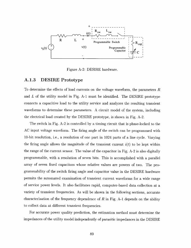
R L( Rsw Lsw
L-- -- - -- --_ __ __ I I-R L +
Programmable Switch R+ cap
vs(t) - v(t) ProgrammableCapacitor
Figure A-2: DESIRE hardware.
A.1.3 DESIRE Prototype
To determine the effects of load currents on the voltage waveform, the parameters R
and L of the utility model in Fig. A-1 must be identified. The DESIRE prototype
connects a capacitive load to the utility service and analyzes the resulting transient
waveforms to determine these parameters. A circuit model of the system, including
the electrical load created by the DESIRE prototype, is shown in Fig. A-2.
The switch in Fig. A-2 is controlled by a timing circuit that is phase-locked to the
AC input voltage waveform. The firing angle of the switch can be programmed with
10-bit resolution, i.e., a resolution of one part in 1024 parts of a line cycle. Varying
the firing angle allows the magnitude of the transient current i(t) to be kept within
the range of the current sensor. The value of the capacitor in Fig. A-2 is also digitally
programmable, with a resolution of seven bits. This is accomplished with a parallel
array of seven fixed capacitors whose relative values are powers of two. The pro-
grammability of the switch firing angle and capacitor value in the DESIRE hardware
permits the automated examination of transient current waveforms for a wide range
of service power levels. It also facilitates rapid, computer-based data collection at a
variety of transient frequencies. As will be shown in the following sections, accurate
characterization of the frequency dependence of R in Fig. A-1 depends on the ability
to collect data at different transient frequencies.
For accurate power quality prediction, the estimation method must determine the
impedances of the utility model independently of parasitic impedances in the DESIRE

hardware. As modeled in Fig. A-2, the DESIRE programmable switch contains para-
sitic resistance and inductance. The load shown in Fig. A-2 is the the programmable
capacitor, modeled with an equivalent series resistance. In the DESIRE prototype,
no extreme effort was expended to minimize these parasitic elements or calibrate the
test capacitances, since the parasitics are likely to depend on time, temperature and
other environmental factors. The parameter estimation scheme described in the next
section does not depend on any a priori knowledge of this kind.
A.1.4 Parameter Estimation and Extrapolation
If measurements are made of v(t), v,(t) and i(t), as indicated in Fig. A-2, the unknown
parameters R and L of the utility model can be estimated. Because the parameters
R and L are unknown,the voltage v,(t) can only be measured when i(t) is zero,
which precludes direct measurement during the transient. For practical purposes, we
assume that vs (t) is shift invariant over a small integer multiple n of the fundamental
period T, i.e. v,(t) a v,(t + nT). By collecting reference waveforms immediately
before performing a transient test, which is easily accomplished with a computerized
data acquisition system, the shift nT above can be made quite small. Note that
the requirement that i(t) = 0 does not imply that the transformer is unloaded. The
transformer load need only be in steady state over the short interval required to collect
vS(t) and perform the transient test. Measurement of i(t) and v(t) during the transient
is straightforward.
A.1.5 Identification of the parameters R and L
Assuming that vs(t) is shift invariant as above, the parameters R and L constrain the
signals v(t), i(t), and v,(t) according to the relationship in Eqn. A.1. In the following,
p represents the differentiation operator d
vs(t) - v(t) = (R + Lp)i(t). (A.1)
The parameters R and L could be found directly from Eqn. A.1 if the continuous

time current waveform were available and could be differentiated accurately. The
measured data, however, consists of the samples i(nTs), v(nTs), and vs(nT,), where
T, is the sampling period. We eliminate the problems associated with measuring
or approximating the derivatives in Eqn. A.1 by introducing the causal, "low-pass"
operator A, with 7 > 0, [10]:
1 p (A.2)1 + pT
Solving Eqn. A.2 for p, we obtain the following:
1-A
Equation A.1 can be reformulated by substitution with Eqn. A.3 to produce a
linear least squares tableau that can be used to estimate R and L:
[T1(vs - v)](t)T 1(A4
=[-TAi i(t), (A.4)
where 01 and 32 are estimates of - and !, respectively. The notation [Ai](t) indicates
the row vector ([Ai](T), [Ai](2T)...[Ai](NT)), where [Ai](t) is the result of applying A
to i(t) at time t. Although A is a continuous time operator, we have found that it
can be applied off-line to linear or zero-order hold interpolations of the finely sampled
quantities with little error. It is desirable to apply A to sampled data for reasons of
implementation. The time constant T associated with A must be determined by the
user. The time constant should be chosen to preserve information content, and also so
that the effects of noise in the regressors and the errors associated with interpolation of
the sampled data are minimized. All of the results presented here were obtained using
T = .002s. In practice, a relatively wide range of values of 7 produces satisfactory
estimates.
Equation A.4 is arranged to minimize the bias in the parameter estimate introduced
by disturbances in the measurements. In particular, the regressors are picked so that
they are low-pass. Unless disturbances are pathologically low-pass, the error in the
filtered regressors will be substantially uncorrelated to the unfiltered right-hand side.

22.900uF
29.800uF
40.400uF
47.200uF
55.300uF
65.900uF
Cap 771.900uF
79.400uF
L R0.00109 1.099
0.00109 1.022
0.00110 0.957
0.00110 0.934
0.00111 0.905
3.00111 0.869
0.00112 0.858
3.00112 0.848
Reet w 1-QuitView 1-4 4
DESIRE
40.0
C 20.0
r 0.0en
-20.0
-40.0
40.0
C 20.0u
U.U
-20.0
-40.0
0.00 Time, ms 4.00
0.00 Time, ms
40.0
C 20.0u
r
r 0.0
en
-20.0
-40.0
40.0
C 20.0u
r
r 0.0
en
-20.0t
-40.0
Capacitor 2
0.00 Time. ms 4.00
Capacitor 4
I I I I I I I
4.00 0.00 Time. ms 4.00
Figure A-3: Screen interaction with DESIRE prototype.
If the disturbances are symmetrically distributed and uncorrelated to the regressors,
for large N the estimates will be unbiased. A more thorough discussion of the role of
noise in this method can be found in [10].
A.1.6 Estimating transient frequency
It is important to associate a frequency f with the parameter R found by the methods
outlined above, as R is a function of frequency. We account for the parasitic elements
in Fig. A-2 by defining quantities Rtot = R + Rsw + Rcap and Ltot = L + Lsw. The
transient frequency f (in Hertz) is given by Eqn. A.5 in terms of these new parameters.
1 1 R2o tf - 27r ý LtotC 4Ltot (A.5)
I @ ... . .
I I I 1 1 I I
U.U

One approach to find the estimate f, therefore, is to first determine the unknown
parameters Rtt, Lot,t and C and then use Eqn. A.5. This technique is preferable to
timing zero crossings, for example, because it is relatively insensitive to noise at the
zero crossings and is independent of the steady state response.
To find the estimates Roto, L-ot, and C, we employ the A-operator substitution
technique to the equation relating i(t) to vs(t) in Fig. A-2:
vs(t) = (Rtot + Ltotp + )i(t). (A.6)
Substitution to eliminate p yields the following equation in terms of the operator
A and its parameter 7.
[T2A2i](t) 2 = [-i + 2Ai - A2i](t) (A.7)
S[ (A 2 - A)v,](t) \3
where K1, &2 and d3 are estimates of Rot, L•t, and , respectively. Equation A.7 isLtot' IC Ltot Esolved in a least-squares sense and the parameter estimates are used to compute the
transient frequency f using Eqn. A.5.
A.1.7 Frequency dependence of R
In [1] and in the experiments in our laboratory, the apparent resistance R was observed
to be an increasing function of the frequency f of the transient. Phenomena that could
explain this observation include, for example, eddy currents induced in conductors
adjacent to current carrying wires and skin effect in the wires themselves.
In [3] the change of resistance due to the skinning effect in a conductor with
cylindrical geometry is given for x <« 1 ("low" frequencies) as
R X4o 1 + (A.8)Rowhere x 192
where x • /f and the constant of proportionality, given explicitly in [3], is related to

the physical properties and geometry of the conductor. Ro is the DC resistance.
From [3], eddy currents in conductive materials adjacent to current carrying wires
produce changes in effective resistance as in Eqn. A.9, which is valid for 0 << 1.
02R R Ro + 27rfLo-6 (A.9)
Here, 0 oc vf. Again, the constant of proportionality is geometry and material
dependent, and can be found analytically for certain geometries.
Assuming that the constants relating x and 0 to Jv are favorably scaled, Equations
A.8 and A.9 suggest the following fitting function, with parameters Ro and 6.
R(f) = Ro + 6f 2 (A.10)
With several estimates •R(f) made at different frequencies, a least-squares solution
for the parameters RT and 6 can be found which satisfies Eqn. A.10. Transient tests at
different frequencies can be automatically conducted by the DESIRE system simply
by programming a range of values for C. It may be possible, based on the value of 6,to determine frequencies above which Eqn. A.10 becomes invalid. However, this was
not investigated in detail here because the purpose is to extrapolate the data to lower
frequencies, and because the collected data at higher frequencies are well interpolated
by Eqn. A.10.
A.1.8 Experimental Results
The test setup used to validate the DESIRE hardware and software consisted of a
single phase 1 kVA isolation transformer connected between phase and neutral of a
three-phase 60 Hz, 30 A per phase, electrical service. A relatively small transformer
was chosen so that it could be removed from service and characterized independently
during development. After the transformer was characterized using the DESIRE sys-
tem, a laser printer with a base plate rating of 7.6 A at 115 VAC RMS was connected
to the transformer. Given the laser printer's remarkable current waveform, we predict

1.1
1.05
1
" 0.95
0.985
0.85
0.875
0.75
070 100 200 300 400 500 600 700 800 900 1000
Frequency, Hertz
Figure A-4: Resistance R as a function of frequency f.
the voltage distortion due to the service parameters R(f) and L.
Figure A-3 shows a screen interaction with the DESIRE system. DESIRE can be
configured to conduct eight transient measurements on a utility connection automat-
ically. The user selects nominal capacitor values which will be connected across the
utility. The estimated capacitor values used during the tests are shown at the far left
hand side of the screen in Fig. A-3. The transient currents during each of the exper-
iments are plotted on the right hand side of the screen for four of the eight different
capacitor values. The user may view either the first or second set of four transient
plots. The estimated values of R and L for the the service model are displayed to the
left of the transient current plots.
Fig. A-4 shows estimated resistance R as a function of transient frequency f (Hz).
The solid line is the interpolation of the data according to the model of Eqn. A.10,and the dashed line shows the extrapolation of the model to lower frequencies. The
estimated inductance L was 1.10 mH.
Fig. A-5 shows a transient current waveform drawn by the printer during operation.
In Fig. A-6, the measured and predicted line voltages are displayed. The data
points show the measured voltage waveform, decimated for clarity. The solid line is a
linear interpolation of the simulation results.
-0
-0
__ .
i -

0
0
15Time, s
Figure A-5: Sample current transient.
The predicted data was obtained using the estimate L, the extrapolation of Eqn. A.10
to 60 Hertz using the data in Fig. A-4, the measured current i(t), and Eqn. A.1.
A.1.9 Conclusions
The DESIRE prototype and analysis software provide a flexible system for charac-
terizing the effective impedance of a utility service connection. This information can
be used for a variety of applications by utilities, and also commercial and industrial
facilities managers. In [13], the nonintrusive load monitor was demonstrated to have
the ability to disaggregate the operating schedule of individual loads given access only
to the aggregate current waveforms at the service entry. With additional knowledge
collected during a one-time (or at least infrequent) examination of the details of a
building's wiring harness, the location of loads on the harness, and the service connec-
tion impedances as determined by the DESIRE system, the nonintrusive load monitor
could provide continuous prediction of the local voltage waveform at points of interest.
We have demonstrated the basis for this power quality monitoring technique in this
paper.
The impedance calculations made by DESIRE could also be used, for example, to
compute the available fault currents at a service connection. This information would

150
100
50
-50
-100
-150
-230-0.04 -0.03 -0.02 -0.01 0 0.01 0.02 0.03 0.04 0.05
Time, s
Figure A-6: Measured and predicted line voltage distortion.
help to verify the proper rating of protection circuitry in the wiring harness. During
our experimentation, we have observed that careful, high sample rate examination
of the transient current waveforms collected by DESIRE reveal additional, very high
frequency ringing that we suspect can be attributed to neglected elements in the utility
model, e.g., inter- and intra-winding capacitances. It is conceivable that additional
information about the utility service impedance could be determined by DESIRE,
which might be useful for determining the propagation of high frequency EMI or
power line carrier modem signals.
A.2 MATLAB Source Code
This is the Matlab source code used for the analysis described above.
meister.m
This is the main driver program; it processes all the data files.
clear M;
I I I I I I

M(1, :) = run2( 'tek00000.csv','refl.csv', 'ref2.csv', 10.0);M(2, :) = run2( 'tek00002.csv','refl.csv', 'ref2.csv', 10.0);M(3, :) = run2( 'tek00004.csv','refl.csv', 'ref2.csv', 10.0);M(4, :) = run2( 'tek00006.csv','refl.csv', 'ref2.csv', 10.0);M(5, :) = run2( 'tek00008.csv',"refl.csv', 'ref2.csv', 10.0);M(6, :) = run2( 'tek00010.csv','refl.csv', 'ref2.csv', 10.0);M(7, :) = run2( 'tek00012.csv','refl.csv', 'ref2.csv', 10.0);M(8, :) = run2( 'tek00016.csv','refl.csv', 'ref2.csv', 10.0);M(9, :) = run2( 'tek00018.csv','refl.csv', 'ref2.csv', 10.0);M(10,:) = run2( 'tek00020.csv','refl.csv', 'ref2.csv', 10.0);M(11,:) = run2( 'tek00020.csv','refl.csv', 'ref2.csv', 10.0);M(12,:) = run2( 'tek00024.csv','refl.csv', 'ref2.csv', 10.0);
'tekO0001.csv',
'tek00003.csv',
'tek00005.csv',
'tek00007.csv',
'tek00009.csv',
'tek0Ol.csv',
'tek00013.csv',
'tek00017.csv',
'tek00019.csv',
'tek00021.csv',
'tek00021.csv',
'tek00025.csv',
f = M(:,1)r = M(:,5);11 = M(:,3);12 = M(:,6);
rob2(r,f);
figure;
subplot(211),plot(f,r, o');v = axis;v(4) = mean(12)*max(r)/mean(r);v(3) = mean(12)*min(r)/mean(r);subplot(212),plot(f,12, o'),axis(v);

run2.m
function qr = run2( fl, f2, f3, f4, Aset )
% Load[t2,y]K(: ,1)[t2,y]
K(: ,1)[t2,y]
K(: ,2)[t2,y]K(:,3)
up the data.= tekload(fl);
= y(:);= tekload(f4);
= K(:,1) - y(:);= tekload(f2);
= y(:);= tekload(f3);
Sy(:);
% Current
% subtract current DC offset setting.
% Vcap
. input voltage waveform.
M = K(1:1000,:);
t = t2(1:1000);
% Zero out the stufffor i = 1:size(M,1)if t(i) < 0.0
M(i,:) = 0.0 *end;
end;
that happens before t = 0.0
M(i,:);
% Scale up the data according to probe settings.
M(:,1) = M(:,1) * Aset / .01;M(:,2) = M(:,2) * 100 / .2;M(:,3) = M(:,3) * 100 / .2;
% analyze the data.tau = .0002;
qr = robme2(M,t,tau);
qr = qr(:)';

robme2.m
% Improved identification procedures for rob-meister's% DESIRE box.
function qr = robme2(M,t,tau)
Volts(:) = M(:,3);
icap(:) = M(:,1);vcap(:) = M(:,2);
% Now apply lambda operators.
li = lsim(1,[tau,1],icap,t);12i = lsim(1,[tau,1],li,t);Iv = isim(1,[tau,1],Volts,t);12v = lsim(l,[tau,l],lv,t);
Q(:,1) = tau * ( li(:) -12i(:));Q(:,2) = tau*tau*12i(:);Q(:,3) = -tau*(lv(:) - 12v(:));rhs(:) = -( icap(:) - 2*li + 12i );
Xsubplot(211),plot(li);%subplot(212),plot(lv);
p = Q \ rhs;
C = p(3)/p(2);L = 1/p(3);
R = p(1)/p(3);
omega = sqrt(1/(L*C)-R*R/(4*L*L)) / (2*pi);
qr(1) = omega;qr(2) = R;qr(3) = L;qr(4) = C;
100
% Do RC
Ivind = isim(l,[tau,l],Volts(:)-vcap(:),t);W(:,1) = tau*li(:);W(:,2) = icap(:)-li(:);
px = W \ (tau*lvind(:));
qr(5) = px(1);qr(6) = px(2);
rob2.m
This file produces the plot of resistance as a function of frequency.
function rob2( hrm, frqm)clear global frq;clear global hr;
frq = frqm;hr = hrm;
global frq;global hr;
xO = [1.0,1.0];x = fsolve('fun', xO)x
clf;plot(frq, hr, 'bo');hold on;
clear global frq;clear global hr;frq = 400:1000;hr = 0 * frq;
global frq;global hr;y = fun(x);plot (frq, y);
% plot data points.
% plot the fit.
101
clear global frq;clear global hr;
frq = 0:400;
hr = 0 * frq;
global frq;global hr;y = fun(x);plot(frq,y,'r-.'); % plot the extrapolation.
y(60)
%title('Resistance as a function of frequency');ylabel('R, Ohms');xlabel('Frequency, Hertz');
tekload.m
This file loads a Tektronix ".CSV" file.
function [x,y]=tekload(name)
fid=fopen(name, 'r');output=fscanf (fid, '%f, f ', [2, infl);x=output(1,:);y=output (2,:);
fclose (fid);
checktime.m
This file is used to check alignment of data files collected at different times.
% Check synchronization signals graphically.
102
clf;clear;
[t,edge] = tekload('tekOO00003.csv');plot (t,edge, 'y+');
hold;
[t,edge] = tekload('tekOO00006.csv');plot (t,edge, 'm+');
[t,edge] = tekload('tek00009.csv');plot(t,edge,'c+');
[t,edge] = tekload('tek00012.csv');plot(t,edge,'r+');
[t,edge] = tekload('tek00015.csv');plot(t,edge,'g+');
[t,edge] = tekload('tek00018.csv');plot (t,edge, 'b+');
[t,edge] = tekload('tek00021.csv');plot (t,edge, 'w+');
[t,edge] = tekload('tek00024.csv');plot (t,edge, 'yx');
[t,edge] = tekload('tek00027.csv');plot (t,edge, 'mx');
[t,edge] = tekload('tek00030.csv');plot(t,edge,'cx');
[t,edge] = tekload('tek00033.csv');plot (t,edge, 'rx');
[t,edge] = tekload('tek00036.csv');plot(t,edge,'gx');
[t,edge] = tekload('tek00039.csv');plot (t,edge, 'bx');
103

[t,edgel = tekload('tekOO042.csv');plot(t,edge, "wx');
[t,edge] = tekload('tekOO045.csv');plot (t,edge, 'yo');
[t,edge] = tekload('tekOO048.csv');plot (t,edge, 'mo );
title('Synchronization Edge Alignment');ylabel('Sync Edge (Volts) );xlabel('Time (s) ');
104

Appendix B
CSIM Simulation Environment
The following document describes a general purpose set of C routines designed to
ease coding of simple simulations. Although not developed for this thesis work, it is
included here because of the applicability to further work on this subject.
B.1 Introduction
CSIM is intended to provide a relatively robust, easy to use simulation environment
for simulation of simple differential equations. Ideally, the user need only express the
differential equation model of a system in C syntax to simulate the system.
This document describes how to translate a simple physical model of the elec-
trical terminal behavior of a lightbulb into the procedures required by CSIM. C is an
inherently flexible language; the discipline and structure needed to create readable
and reliable programs comes from the programmer, not the language. This example
should be regarded not only as documentation of CSIM itself, but also as a paradigm
of the user coded routines.
CSIM contains portions of code which are an adaptation of the routines published
in Numerical Recipes in C (Press, Flannery, et. al). Those routines are NOT the
public domain and require the purchase of Numerical Recipes in C for licensed use.
105

B.2 General description of the integration procedure
CSIM is a numerical integrator based on a Runge-Kutta procedure. Local truncation
errors are estimated at each step using a lower order embedded method, and the step
size is adjusted so that the errors are bounded by a user selectable e. The default
is to restrict relative errors to f = le - 6, but the value can be changed by calling
setepsilon. The variable step size algorithm is executed between evenly spaced "grid
points". The idea is to simulate as closely as possible actual experimental conditions
- for reasons of implementation, data are usually collected at a constant sampling rate
determined before the experiment is performed and independent of the local frequency
content of the results.
There are two procedures that the user must code to perform a simulation. The
third is optional.
* Derivatives as a function of states and inputs
* Mapping of states, etc. to outputs
* A routine introducing discontinuous changes in state/topology
In translating a model to C code, then, the state matrix would be expressed in the
first procedure, the output matrix in the second procedure, and features like switches
and diodes and relays would be contained in the third procedure. We will consider a
simple example that requires all three routines.
B.3 A physical description of a lightbulb
An incandescent light bulb is a thin wire surrounded by a protective atmosphere
contained in a glass envelope. When the bulb is connected to the mains, the resulting
current flow rapidly heats the filament until the electrical power deposited in the
filament equals the radiative flux emanating from the bulb. We will model the filament
as a black body, with the consequence that the radiant power Prad = alT4 . Here T
is the filament temperature. The electrical power deposited in the filament is simply
106

Pe = IV. We assume that the thermo and thermoelectric constitutive relations of the
filament itself are Pfil = a2T and Rfil = a3 + a4T. Specifically, we assume that a
heat capacity is a sufficient thermal description of the filament, and that the filament
has a linearly increasing resistance as a function of temperature. Further, suppose
(mostly for purposes of illustration) that the filament might undergo an unstable
sublimation process if the filament exceeds a certain critical temperature. This is
not an unreasonable assumption, because a "hot spot" on the filament will sublimate
faster than the rest of the filament, and subsequently will get even hotter.
Differentiating the first law of thermodynamics (conservation of energy) with re-
spect to time, we have Pfil = Pe - Prad, or, equivalently.
dT V 2
a2 alT4 (B.1)dt a3 + a4T
This is our equation of state, which must be translated to C in the first routine
required by CSIM.
In the power monitoring scenario, V = V(T) = 179 sin 377t, and we are interested
in the current. Therefore the output relationship is
(t) = (B.2)
a3 + a4T
Furthermore, we will model the sublimation as severing the filament when the
filament temperature exceeds a certain critical temperature a5 . That is, I(to + t) = 0
for all positive t if T(to) > as.
B.4 C Code
The C code to implement the model described above is reproduced and explained
below. A clean copy without additional comments and editorializing is in Section 7.
/*** Simulation of a lightbulb.
#include <stdio.h>
107

#include <math.h>#include "integrate .h"#include "csim.h"
The include files in quotes are part of the CSIM routines and must be in the
current working directory. The other include files are required to use functions
like printf and cos. The sensible way to organize the list of include files is
with the standard includes (with "<>") first and the "local" includes next.
/* Prototypes. */void burnout(double , double , double , double ); 10void derivs(double , double , double , double );void output(double , double , double , double );
Next come the "prototypes." Prototypes are declarations of a function's
expected return and argument types that allow the compiler to do a more
thorough job of making sure that the functions are used as anticipated. All
functions should be prototyped.
static char *output_file = "results. out";
Here is the main program. The operating system starts the thread of execution
here.
int main(void){
FILE *f = fopen(outputfile, "w");static double s[10],ds[10],aux[10];static double par[10]; 20
if(f == NULL) {printf("Problem opening file... .\n");return 1;
108

}In this first part of main, a file to put the results in is opened and arrays to
store the state (s), derivative (ds), some auxiliary variables (aux) and the
parameters of the model (par) are created. Although we only have 1 state
variable, there is no harm done in being on the safe side. Note that the array
you allocate here must have AT LEAST N + 1 elements if there are N states,
because the convention used in the simulator code is to begin indexing arrays at
1 not 0. The auxiliary variables are available for the communication of any
interesting quantities between the three routines. In the lightbulb example, the
auxiliary variables are used to store the state of the filament (broken or not)
and the current. Whenever a file is opened, check to be sure that the pointer is
valid.
#ifndef QUIETprintf("Simulating lightbulb... \n");
#endif30
filestore init (f);
You might want to run the simulator later without seeing a lot of messages
(for example, if you want to run it in a script). That's the reason for the
preprocessor directives on lines 27 and 29. If you have debugging "printf's",bracket them with an #ifdef DEBUG. The function call on line 31 just tells the
informs the file storage system of the file we'd like to use. On line 111,filestore will write to this file.
/ * Some parameters. */par[l] = le-8;par[2] = 1.0;par[3] = 2;par[4] = .05;par[5] = 350;
/ * Initialize all routines. */ 40derivs(INITIALIZE,par,ds,aux);output (INITIALIZE, par,ds,aux);
109

burnout (INITIALIZE,par,ds,aux);
Here's where the three functions that must be written by the user are
initialized. The second argument, which is normally a state vector, is in this
special circumstance a vector with any initialization information that the
routines might need. In this case, the routines only need to be informed of the
parameters to use for the simulation.
simulate(s,ds,aux,1,.0002,2000,output,derivs,burnout);fclose(f);
#ifndef QUIETprintf("Results are in %s....\n", output_file);printf("Output variables are 1:Time 2:Temperature 3:Current\n");5o
#endifreturn 0;
}
Next, we call the simulate procedure that's part of the CSIM package. The
arguments (from left to right) are the state vector, the derivatives, the auxiliary
variables, the number of state variables, the grid time step, the number of
points to simulate, and the output mapping function, the derivatives function,
and the discontinuous state/topology change function. If you don't need a
function like burnout for your simulation, you can pass an appropriately cast
NULL instead. After simulating, the output file is closed and the program exits.
#define I (aux[1])#define fil (aux[2])#define T (s[1])#define dTdt (ds[1])
These defines just establish a standard map between our equations and the state
and auxiliary vectors. We declare here, for example, that the temperature T is
to be stored in the state s[1].
/* 60** Derivatives,/
110

void derivs(double t, double s[], double ds[], double aux[])
{static double al,a2,a3,a4;
double Pe, Prad, V;
if(t == INITIALIZE) {al = s[1]; 70a2 = s[2];a3 = s[3];a4 = s[4];return;
}Here is the beginning of the derivatives routine, one of the functions that must
be be written by the user. The arguments of the three user written routines are
all the same; time, states, derivatives, and auxiliary variables. Notice the
initialization code. This is where the parameters passed as states (on line 40)
are "remembered" by the derivatives function. The static variables al..a4 are
not allocated off the stack; they retain their values between calls and have local
scope.
if(t == ZEROSTATE) {fil = 1; /* Filament is intactI = 0; /* No currentT = 20.0; /* Start at room temperature */ soreturn;
}
In this segment of code, the derivatives routine is asked to set the state vector
to its initial conditions. You could do this in main(), if you so desired, and
then this segment of code would do nothing but return.
V = 179*sin(377*t); /* Excitation */
if(fil) {I = V/(a3+a4*T); /* Constitutive law */Pe = I*V;
} else {Pe = 0.0; /* Broken filament == No Pe 90
111

I = 0.0;
}
Prad = al*T*T*T*T; /* Stefan-Boltzman law */dTdt = (Pe-Prad)/a2; / * Heat/Temp constitutive relation + 2nd law */
I
The rest of the derivatives routine is nothing more that the equations that were
developed for the lightbulb. If you believe in physics and the approximations
that were made, we should get something that looks just like a lightbulb.
/*** Output mapping 100
void output(double t, double s[], double ds[], double aux[]){
static double col[5];
if( t == INITIALIZE) return;
Here's the output routine. Note that this particular output function doesn't
require any initialization information, but it still detects the t == INITIALIZE
condition. This is important. If you don't do it, your output file will have
spurious data on the first line.
col[1] = t;col[2] = T;col[3] = I; 110
filestore(col, 3);
I
112

The rest of the output procedure is very simple. It simply puts the time in the
first column, the temperature in the second column, and the current in the third
column. Note that we use the current which was already compute for use in the
derivs() function. It is communicated to the output function via the auxiliary
variables. filestore sends the row out to the file pointer we opened up in
main(). The second argument to filestore is the number of columns.
** Discontinuous state/model changes
void burnout( double t, double s[], double ds[], double aux[]) 120
{static double a5;
if( t == INITIALIZE) {a5 = s[5];return;
}Here's the "discontinuous state/model changing routine". Very simply, this is
just a function which is guaranteed to be called only on the grid. The user
supplied function derivs(), in contrast, can be called at any time. You can
use this routine to set "initial conditions" in the middle of a simulation. If you
have states that are not smooth, like ideal diodes, you can approximately
simulate the system by putting your switching logic here.
if(T > a5) {fil = 0; / * Filament is broken */ 130
I = 0.0; /* no current */}
}
113

In this case, we check to see if the bulb temperature has exceed some arbitrary level.
At this level, it is postulated that the filament's electrical constituitive relation will
become discontinuous i.e. the bulb will burn out. This state of affairs is communicated
back to the derivs() routine via the auxiliary variables.
B.5 Make File
In order for the CSIM source code to be appropriately compiled with the file contain the
user written description of the simulation, a make file should be used. The lightbulb
simulator can be compiled with the command make -f lightbulb.make, which pro-
duces an executable file call lightbulb in the current working directory. The make
file lightbulb.make follows.
lightbulb : lightbulb.o integrate.o csim.o nrutil.ogcc -o lightbulb lightbulb.o integrate.o csim.o nrutil.o -lm
lightbulb. o : lightbulb. cgcc -c -Wall lightbulb.c
nrutil.o: nrutil.c nrutil.hgcc -c nrutil.c
csim.o: csim.c csim.hgcc -c csim.c
integrate.o: integrate.c integrate.hgcc -c integrate.c
To make your own make file, simply replace every instance of lightbulb with foo
where foo is the name of the .c file containing your simulation.
114

40
30
20
10
0
-10
-20
-30
-4d
0 0.05 0.1 0.15 0.2 0.25 0.3 0.35 0.4
Figure B-1: Simulated light bulb current
B.6 Results
The program lightbulb made with the model, code, and make file above simulates
correctly and produces some plausible waveforms. The current as a function of time
is shown in Figure B-1. The filament temperature is shown in Figure B-2. The point
at which the filament "burns out" is clear.
115

0 0.05 0.1 0.15 0.2 0.25 0.3 0.35 0.4
Figure B-2: Simulated light bulb temperature
116
400
350
300
250
200
150
100
50
0

B.7 lightbulb.c
** Simulation of a lightbulb.
#include <stdio.h>#include <math.h>#include "integrate .h"#include "csim.h"
/ * Prototypes. */void burnout(double, double, double, double); 10void derivs(double, double, double, double);void output(double, double, double, double);
static char *output file = "results. out";
int main(void){
FILE *f = fopen(outputfile, "w");static double s[10],ds[10],aux[10];static double par[10]; 20
if(f == NULL) {printf("Problem opening file.. .\n");return 1;
}
#ifndef QUIETprintf("Simulating lightbulb... \n");
#endif30
filestore_init(f);
/ * Some parameters. */par[l] = le-8;par[2] = 1.0;par[3] = 2;par[4] = .05;par[5] = 350;
/ * Initialize all routines. */ 40derivs(INITIALIZE,par,ds,aux);output(INITIALIZE,par,ds,aux);
117

burnout (INITIALIZE,par,ds,aux);
simulate(s,ds,aux, 1,.0002,2000,output,derivs,burnout);fclose(f);
#ifndef QUIETprintf("Results are in %s... \n", output file);printf("Output variables are 1:Time 2:Temperature
#endifreturn 0;
}#undef N
#define I#define fil#define T#define dTdt
3: Current\n");50
(aux[1])(aux[2])
(s[1])(ds[1])
** Derivatives
void derivs(double t, double s[], double ds[], double aux[]){
static double al,a2,a3,a4;
double Pe, Prad, V;
if(t == INITIALIZE) {al = s[1];a2 = s[2];a3 = s[3];a4 = s[4];return;
if(t == ZEROSTATE) {fil = 1;I = 0;T = 20.0;return;
}
V = 179*sin(377*t);
/ * Filament is intact/* No current *// * Start at room temperature */
/ * Excitation
118

if(fil) {I = V/(a3+a4*T); /* Constitutive law */Pe = I*V; 90
} else {Pe = 0.0; /* Broken filament == No Pe */I = 0.0;
}
Prad = al*T*T*T*T; /* Stefan-Boltzman lawdTdt = (Pe-Prad)/a2; /* Heat/Temp constitutive relation + 2nd law */
100
** Output mapping
void output(double t, double s[], double ds[], double aux[]){
static double col[5];
if( t == INITIALIZE) return;
col[l] = t; 110co1[2] = T;col [3]= I;
filestore(col, 3);}
** Discontinuous state/model changes 120
void burnout( double t, double s[], double ds[], double aux[]){
static double a5;
if( t == INITIALIZE) {a5 = s[5];return;
}130
119

if(T > a5) {fil = 0;I = 0.0;
}
/* Filament is broken *// * no current
120

B.8 Integration and Utility Codes
The following code may contain portions derived from Numerical Recipes
/*
csim. c
C Simulation code.
Author: Steven R. ShawDate : 9/1/96
Note all revisions after 26 Dec 1996 below:
#include <stdio.h>#include "integ.h"#include "csim.h"
/* Prototype */void filestore_(double [], int , FILE *);
/* Relative precision */static double __eps = le-6;
void simulate(doubledouble di[],double aux[],int n,double H,long L,void (*store)void (*derivs)void (*ongrid)
i[], /* State Vector./* Derivative Vector./* Auxilliary Variables./* Number of states./* Grid./* Number of points.
(double, double [], double(double, double [], double(double, double [], double
*/*/*/*/
*/double []),double []),double [])
long k;
int nok,nbd;
(*derivs)(ZEROSTATE,i,di,aux);
for(k = 1; k <= L; k++) {
/* Evaluate derivatives on grid prior to storage. */(*derivs)((k-1)*H,i,di,aux);
/* Do something on the grid. */
if( ongrid != NULL )
121

(*ongrid)((k-1)*H,i,di,aux);
/* Store. */
(*store)((k-1)*H,i,di,aux);
/* Integrate a step */odeint(i, aux, n, (k-l)*H, (k)*H, __eps, H,0.0, &nok, &nbd, derivs, rkqs);
}
Interface to set the relative precision.
void setepsilon( double precision ){_eps = precision;
}
/*Initialize file storage tools
void filestore_init(FILE *f){
filestore_(NULL,O,(FILE *)f);}
void filestore(double i[], int n){
filestore_(i,n,(FILE *)NULL);}
** Just pass a vector to me.
void filestore_(double s[], int n, FILE *M){
static FILE *z;int j;
if(M == NULL) {for(j = 1; j < n; j++)
fprintf(z, "%.4e\t", s[j]);fprintf(z, "Y.4e\n", s[n]);
} else z = M;}
122

** csim.h
** Note any changes after 26 Dec 1996 Below:**
** * Added definition of M_PI since C6 include files do** not define it... Jan 1997.
void simulate(double i[],
double di[],
double aux[],int n,double H,
long L,
void (*store)(double,double [], double [], double []),
void (*derivs)(double, double [], double [], double []),
void (*ongrid)(double, double [], double [], double []));
void filestore_init(FILE *f);
void filestore(double row[], int n);
void setepsilon(double eps);
#define INITIALIZE (-1)
#define ZEROSTATE (-2)
/* Make C6 compliant. SRS */#ifndef M_PI
#define M_PI (3.1415926535)#endif
123

The following code may contain portions derived from Numerical Recipes
integ.c
THIS FILE CONTAINS CODE FROM NUMERICAL RECIPESNUMERICAL RECIPES COPYRIGHT APPLIES
SRS
List all revision after 26 Dec 1996 below:
*/
#include <math.h>
#define NRANSI#include "nrutil.h"
#include "integ.h"
#define FMIN(a,b) (((a) < (b)) ? (a) : (b))
#define FMAX(a,b) (((a) > (b)) ? (a) : (b))#define SIGN(a,b) (((b) < 0) ? (-(a)) : (a))
#define vector(a,b) dvector(a,b)#define free_vector(a,b,c) freedvector(a,b,c)
#define MAXSTP 10000#define TINY 1.0e-30
/* Prototype */
void rkck(double y[],double dydx [] ,double aux[] ,int n,double x,
double h,
double yout [] ,double yerr[] ,void (*derivs)(double, double [], double [], double []));
/* Code starts here */
void odeint(double ystart[],double aux[],int nvar,double xl,double x2,double eps,double hl,
124

double hmin,int *nok,int *nbad,void (*derivs)(double, double [], double [], double []),void (*rkqs)(double [],
double [],double [],int,
double *,double,
double,
double [],double *,double *,void (*)(double, double [], double [1, double [])))
{int nstp,i;double x,hnext,hdid,h;
double *yscal,*y,*dydx;
yscal=vector(1,nvar);
y=vector(1,nvar);dydx=vector(1,nvar);
x=xl;
h=SIGN(hl,x2-x1);
*nok = (*nbad) = 0;for (i=l;i<=nvar;i++) y[i]=ystart[i];
for (nstp=l;nstp<=MAXSTP;nstp++) {(*derivs)(x,y,dydx,aux);
for (i=l;i<=nvar;i++)
yscal[i]=fabs(y[il)+fabs(dydx[i]*h)+TINY;
if ((x+h-x2)*(x+h-xl) > 0.0) h=x2-x;(*rkqs)(y,dydx,aux,nvar,&x,h,eps,yscal,&hdid,&hnext,derivs);
if (hdid == h) ++(*nok); else ++(*nbad);if ((x-x2)*(x2-xl) >= 0.0) {for (i=l;i<=nvar;i++) ystart[i]=y[i];
free_vector(dydx,l,nvar);
free vector(y,l,nvar);free-vector(yscal,l,nvar);
return;
if (fabs(hnext) <= hmin) nrerror("Step size too small in odeint");h=hnext;
}nrerror("Too many steps in routine odeint");
#undef MAXSTP#undef TINY
#undef NRANSI
125

#define NRANSI#define SWAP(a,b) {temp=(a);(a)=(b);(b)=temp;}
void gaussj(double **a, int n, double **b, int m){
int *indxc,*indxr,*ipiv;int i,icol,irow,j,k,l,ll;double big,dum,pivinv,temp;
indxc=ivector(1,n);indxr=ivector( ,n);ipiv=ivector(1,n);for (j=l;j<=n;j++) ipiv[j]=0;for (i=l;i<=n;i++) {big=0.0;for (j=1;j<=n;j++)
if (ipiv[j] != 1)for (k=l;k<=n;k++) {if (ipiv[k] == 0) {if (fabs(a[j][k]) >= big) {big=f abs (a[j] [k] ) ;irow=j;icol=k;
}} else if (ipiv[k] > 1) nrerror("gaussj: Singular Matrix-l");
}++(ipiv[icol]);if (irow != icol) {
for (1=1;l<=n;l++) SWAP(a[irow] [1],a[icol] [1])for (1=1 ;1<=m;l++) SWAP(b[irow] [1] ,b[icol] [1])
}indxr [i=irow;indxc[i] =icol;if (a[icol] [icol] == 0.0) nrerror("gaussj: Singular Matrix-2");pivinv=1.0/a[icol] [icol] ;a[icol] [icol]=1.0;for (1=1;l<=n;l++) a[icol][1] *= pivinv;for (l=1;l1<=m;l++) b[icol] [1] *= pivinv;for (11=1;ll<=n;ll++)if (11 != icol) {
dum=a [11] [icol] ;a[ll] [icol]=0.0;for (1=1;l<=n;l++) alll] [1] -= a[icol] [l]*dum;for (l=1;l<=m;l++) b[11] [11 -= b[icol] [l]*dum;
}}for (1=n;l>=1;l--) {if (indxr[l] != indxc[l])for (k=l;k<=n;k++)
SWAP(a[k] [indxr[l]],a[k] [indxc [1]]);
free_ivector(ipiv,1,n);free_ivector(indxr, ,n);free_ivector(indxc,1,n);
126

}#undef SWAP#undef NRANSI
#define NRANSI#define SAFETY 0.9#define PGROW -0.2#define PSHRNK -0.25#define ERRCON 1.89e-4
void rkqs(double y[] ,double dydx[] ,double aux[],int n,double *x,double htry,double eps,double yscal[] ,double *hdid,double *hnext,void (*derivs)(double, double [], double [], double []))
void rkck(double y[],double dydx[],double aux[] ,int n,double x,double h,double yout[]l,double yerr[],void (*derivs)(double, double [], double [],double[]));
int i;double errmax,h,htemp,xnew,*yerr,*ytemp;
yerr=vector(l,n);ytemp=vector(l,n);h=htry;for (;;) {
rkck(y,dydx,aux,n,*x,h,ytemp,yerr,derivs);
errmax=0.0;for (i=l;i<=n;i++) errmax=FMAX(errmax,fabs(yerr[i]/yscal[i]));errmax /= eps;if (errmax <= 1.0) break;
htemp=SAFETY*h*pow(errmax,PSHRNK);h=(h >= 0.0 ? FMAX(htemp,0.1*h) : FMIN(htemp,0.1*h));
xnew=(*x)+h;if (xnew == *x) nrerror("stepsize underflow in rkqs");
if (errmax > ERRCON) *hnext=SAFETY*h*pow(errmax,PGROW);
else *hnext=5.0*h;
*x += (*hdid=h);
for (i=l;i<=n;i++) y[i]=ytemp[i];free_vector(ytemp,l,n);
127

free_vector(yerr,l,n);
}#undef SAFETY#undef PGROW
#undef PSHRNK
#undef ERRCON
#undef NRANSI
#define NRANSI
void rkck(double y[],
double dydx[],
double aux[],
int n,double x,
double h,
double yout[],double yerr[],void (*derivs)(double, double [], double [], double []))
int i;
static double a2=0.2,a3=0.3,a4=0.6,a5=1.0,a6=0.875,b21=0.2,
b31=3.0/40.0,b32=9.0/40.0,b41=0.3,b42 = -0.9,b43=1.2,
b51 = -11.0/54.0, b52=2.5,b53 = -70.0/27.0,b54=35.0/27.0,b61=1631.0/55296.0,b62=175.0/512.0,b63=575.0/13824.0,b64=44275.0/110592.0,b65=253.0/4096.0,cl=37.0/378.0,
c3=250.0/621.0,c4=125.0/594.0,c6=512.0/1771.0,
dc5 = -277.00/14336.0;double dcl=cl-2825.0/27648.0,dc3=c3-18575.0/48384.0,
dc4=c4-13525.0/55296.0,dc6=c6-0.25;
double *ak2,*ak3,*ak4,*ak5,*ak6,*ytemp;
ak2=vector(1,n);
ak3=vector(l,n);
ak4=vector(l,n);
ak5=vector(l,n);
ak6=vector(l,n);
ytemp=vector(l,n);
for (i=l;i<=n;i++)
ytemp[i]=y[i]+b21*h*dydx[i];
(*derivs)(x+a2*h,ytemp,ak2,aux);
for (i=l;i<=n;i++)
ytemp[i]=y[i]+h*(b31*dydx[i]+b32*ak2[i]);
(*derivs)(x+a3*h,ytemp,ak3,aux);
for (i=l;i<=n;i++)
ytemp[i]=y[i]+h*(b41*dydx[i]+b42*ak2[i]+b43*ak3[i]);
(*derivs)(x+a4*h,ytemp,ak4,aux);
for (i=l;i<=n;i++)
ytemp[i]=y[i]+h*(b51*dydx[i]+b52*ak2[i]+b53*ak3[i]+b54*ak4[i]);(*derivs)(x+a5*h,ytemp,ak5,aux);
for (i=1;i<=n;i++)ytemp[i]=y[i]+h*(b61*dydx[i]+b62*ak2[i]+b63*ak3[i]+b64*ak4[i]+b65*ak5[i]);
(*derivs)(x+a6*h,ytemp,ak6,aux);
for (i=l;i<=n;i++)
128

yout [i]=y [i]+h* (cl*dydx [i]+c3*ak3 [i]+c4*ak4 [i]+c6*ak6 [i]);for (i=l; i<=n;i++)
yerr[i]=h*(dcl*dydx[i]+dc3*ak3[i]+dc4*ak4 [i]c[+dcak5 [i] 6*ak6[i]);free_vector(ytemp,1,n);free_vector(ak6,1,n);free_vector(ak5,1,n);free_vector(ak4,1,n);free_vector(ak3,1,n);free_vector(ak2, 1,n);
#undef NRANSI
129

integ.h
Note all revision after 26 Dec 1996 below:
void odeint(double ystart[] ,double aux[],int nvar,double xi,double x2,double eps,double hl,double hmin,int *nok,int *nbad,void (*derivs)(double, double [], double [], double []),void (*rkqs)(double [1,
double [],double [1,int,double *,double,double,double [],double *,double *,void (*)(double, double [], double [], double [])));
void rkqs(double y[],double dydx [],double auxE],int n,double *x,double htry,double eps,double yscal [] ,double *hdid,double *hnext,void (*derivs)(double, double [], double [], double []));
void gaussj(double **a, int n, double **b, int m);
130

The following code may contain portions derived from Numerical Recipes
nrutil.c
THIS FILE CONTAINS MODIFIED CODE FROM NUMERICAL RECIPES
Numerical Recipes copyright restrictions may apply.
Note any revision after 26 Dec 1996 below:
1. all instances of "float" explicitly replaced with"double" (SRS,12/27/96)
*/
CAUTION: This is the ANSI C (only) version of the Numerical Recipesutility file nrutil.c. Do not confuse this file with the same-namedfile nrutil.c that is supplied in the 'misc' subdirectory.*That* file is the one from the book, and contains both ANSI andtraditional K&R versions, along with #ifdef macros to select thecorrect version. *This* file contains only ANSI C.
*/#include <stdio.h>
#include <stdiodef.h>
/* #include <stddef.h>*/#include <stdlib.h>
#define NR_END 1#define FREE_ARG char*
void nrerror(char error_text[])/* Numerical Recipes standard error handler */{fprintf(stderr,"Numerical Recipes run-time error...\n");fprintf(stderr,"%s\n",errortext);
fprintf(stderr,"...now exiting to system...\n");exit(l);}
double *vector(long nl, long nh)/* allocate a double vector with subscript range v[nl..nh] */{double *v;
v=(double *)malloc((sizet) ((nh-nl+l+NR_END)*sizeof(double)));if (!v) nrerror("allocation failure in vector()");
131

return v-nl+NR_END;}
int *ivector(long nl, long nh)/* allocate an int vector with subscript range v[nl..nh] */{int *v;
v=(int *)malloc((size_t) ((nh-nl+l+NREND)*sizeof(int)));if (!v) nrerror("allocation failure in ivector()");return v-nl+NR_END;}
unsigned char *cvector(long nl, long nh)/* allocate an unsigned char vector with subscript range v[nl..nh] */{unsigned char *v;
v=(unsigned char *)malloc((size_t)((nh-nl+l+NR_END)*sizeof(unsigned char)));
if (!v) nrerror("allocation failure in cvector()");return v-nl+NR_END;}
unsigned long *lvector(long nl, long nh)/* allocate an unsigned long vector with subscript range v[nl..nh] */{unsigned long *v;
v=(unsigned long *)malloc((size_t) ((nh-nl+l+NR_END)*sizeof(long)));if (!v) nrerror("allocation failure in lvector()");return v-nl+NR_END;}
double *dvector(long nl, long nh)/* allocate a double vector with subscript range v[nl..nh] */{double *v;
v=(double *)malloc((size_t) ((nh-nl+l+NR_END)*sizeof(double)));if (!v) nrerror("allocation failure in dvector()");return v-nl+NR_END;}
double **matrix(long nrl, long nrh, long ncl, long nch)/* allocate a duble matrix with subscript range m[nrl..nrh] [ncl..nch] */{long i, nrow=nrh-nrl+l,ncol=nch-ncl+1;double **m;
/* allocate pointers to rows */m=(double **) malloc((size_t)((nrow+NR_END)*sizeof(double*)));if (!m) nrerror("allocation failure 1 in matrix()");m += NREND;
132

m -= nrl;
/* allocate rows and set pointers to them */
m[nrl]=(double *) malloc((size_t)((nrow*ncol+NR_END)*sizeof(double)));
if (!m[nrl]) nrerror("allocation failure 2 in matrix()");
m[nrl] += NR_END;
m[nrl] -= ncl;
for(i=nrl+1;i<=nrh;i++) m[i]=m[i-1]+ncol;
/* return pointer to array of pointers to rows */return m;
}
double **dmatrix(long nrl, long nrh, long ncl, long nch)
/* allocate a double matrix with subscript range m[nrl..nrh] [ncl..nch] */
{long i, nrow=nrh-nrl+l,ncol=nch-ncl+1;
double **m;
/* allocate pointers to rows */
m=(double **) malloc((sizet)((nrow+NREND)*sizeof(double*)));
if (!m) nrerror("allocation failure 1 in matrix()");
m += NREND;
m -= nrl;
/* allocate rows and set pointers to them */m[nrl]=(double *) malloc((sizet)((nrow*ncol+NR_END)
*sizeof(double)));
if (!m[nrl]) nrerror("allocation failure 2 in matrix()");m[nrl] += NREND;
m[nrl] -= ncl;
for(i=nrl+1;i<=nrh;i++) m[i]=m[i-1]+ncol;
/* return pointer to array of pointers to rows */return m;
}
int **imatrix(long nrl, long nrh, long ncl, long nch)
/* allocate a int matrix with subscript range m[nrl..nrh] [ncl..nch] */{long i, nrow=nrh-nrl+l,ncol=nch-ncl+1;
int **m;
/* allocate pointers to rows */
m=(int **) malloc((size_t) ((nrow+NREND)*sizeof(int*)));
if (!m) nrerror("allocation failure 1 in matrix()");m += NR_END;
m -= nrl;
/* allocate rows and set pointers to them */m[nrl]=(int *) malloc((size_t)((nrow*ncol+NR_END)*sizeof(int)));
133

if (!m[nrl]) nrerror("allocation failure 2 in matrix()");m[nrl] += NR_END;m[nrl] -= ncl;
for(i=nrl+1;i<=nrh;i++) m[i]=m[i-1]+ncol;
/* return pointer to array of pointers to rows */return m;}
double **submatrix(double **a, long oldrl, long oldrh, long oldcl, long oldch,long newrl, long newcl)/* point a submatrix [newrl..][newcl..] to a[oldrl..oldrh][oldcl..oldch] */{long i,j,nrow=oldrh-oldrl+l,ncol=oldcl-newcl;double **m;
/* allocate array of pointers to rows */m=(double **) malloc((sizet) ((nrow+NR_END)*sizeof(double*)));if (!m) nrerror("allocation failure in submatrix()");m += NR_END;m -= newrl;
/* set pointers to rows */for(i=oldrl,j=newrl;i<=oldrh;i++,j++) m[jl=a[i]+ncol;
/* return pointer to array of pointers to rows */return m;}
double **convert_matrix(double *a, long nrl, long nrh, long ncl, long nch)/* allocate a double matrix m[nrl..nrh][ncl..nch] that points to the matrixdeclared in the standard C manner as a[nrow] [ncol], where nrow=nrh-nrl+land ncol=nch-ncl+l. The routine should be called with the address&a[O] [0] as the first argument. */{long i,j,nrow=nrh-nrl+l,ncol=nch-ncl+l;double **m;
/* allocate pointers to rows */m=(double **) malloc((size_t) ((nrow+NREND)*sizeof(double*)));if (!m) nrerror("allocation failure in convertmatrix()");m += NR_END;m -= nrl;
/* set pointers to rows */m[nrl]=a-ncl;for(i=l,j=nrl+l ;i<nrow;i++,j++) m[j=m[j -1]+ncol;/* return pointer to array of pointers to rows */return m;}
double ***f3tensor(long nrl, long nrh, long ncl, long nch, long ndl, long ndh)/* allocate a double 3tensor with range t[nrl..nrh] [ncl..nch] [ndl..ndh] */
134

{long i,j,nrow=nrh-nrl+l,ncol=nch-ncl+l,ndep=ndh-ndl+1;double ***t;
/* allocate pointers to pointers to rows */t=(double ***) malloc((size_t)((nrow+NR_END)*sizeof(double**)));if (!t) nrerror("allocation failure 1 in f3tensor()");t += NREND;t -= nrl;
/* allocate pointers to rows and set pointers to them */t [nrl]=(double **) malloc((size_t)((nrow*ncol+NR_END)*
sizeof(double*)));if (!t[nrl]) nrerror("allocation failure 2 in f3tensor()");t[nrl] += NREND;t[nrl] -= ncl;
/* allocate rows and set pointers to them */t [nrl] ncl] =(double *) malloc((size_t) ((nrow*ncol*ndep+NR_END)
*sizeof(double)));if (!t[nrl] [ncl]) nrerror("allocation failure 3 in f3tensor()");t[nrl][ncl] += NR_END;t[nrl][ncl] -= ndl;
for(j=ncl+l;j<=nch;j++) t[nrl] [j]=t[nrl] [j-1]+ndep;for(i=nrl+; i<=nrh;i++) {t[i]=t[i-l]+ncol;t [i][ ncl]=t [i-1] [ncl]+ncol*ndep;for(j=ncl+l;j<=nch;j++) t[i] [j]=t[i] [j-1]+ndep;}
/* return pointer to array of pointers to rows */return t;}
void free_vector(double *v, long nl, long nh)/* free a double vector allocated with vector() */{free((FREE_ARG) (v+nl-NR_END));
}
void freeivector(int *v, long nl, long nh)/* free an int vector allocated with ivector() */
{free((FREE_ARG) (v+nl-NR_END));}
void free_cvector(unsigned char *v, long nl, long nh)/* free an unsigned char vector allocated with cvector() */{free((FREE_ARG) (v+nl-NR_END));}
void freeilvector(unsigned long *v, long nl, long nh)
135

/* free an unsigned long vector allocated with Ivector() */
{free((FREE_ARG) (v+nl-NR_END));
}
void free_dvector(double *v, long nl, long nh)
/* free a double vector allocated with dvector() */
{free((FREE_ARG) (v+nl-NREND));}
void free_matrix(double **m, long nrl, long nrh, long ncl, long nch)
/* free a double matrix allocated by matrix() */
{free((FREE_ARG) (m[nrl]+ncl-NREND));free((FREEARG) (m+nrl-NREND));
}
void free_dmatrix(double **m, long nrl, long nrh, long ncl, long nch)
/* free a double matrix allocated by dmatrix() */
{free((FREEARG) (m[nrll+ncl-NREND));free((FREEARG) (m+nrl-NREND));
}
void free_imatrix(int **m, long nrl, long nrh, long ncl, long nch)/* free an int matrix allocated by imatrix() */
{free((FREE_ARG) (m[nrl]+ncl-NREND));free((FREE_ARG) (m+nrl-NREND));
}
void free_submatrix(double **b, long nrl, long nrh, long ncl, long nch)/* free a submatrix allocated by submatrix() */
{free((FREEARG) (b+nrl-NR END));}
void free_convert_matrix(double **b, long nrl, long nrh, long ncl, long nch)
/* free a matrix allocated by convertmatrix() */
{free((FREEARG) (b+nrl-NR_END));
}
void freef3tensor(double ***t, long nrl, long nrh, long ncl, long nch,long ndl, long ndh)/* free a double f3tensor allocated by f3tensor() */
{free((FREEARG) (t[nrl] [ncl] +ndl-NREND));
free ( (FREE-ARG) (t[nrl] +ncl-NREND));free((FREEARG) (t+nrl-NREND));
}
136

The following code may contain portions derived from Numerical Recipes
/*nrutil.h
THIS FILE CONTAINS MODIFIED CODE FROM NUMERICAL RECIPESNumerical Recipes Copyright may apply.
Note any modifications after 26 Dec 1996 below:
1. Explictly replaced all floats with doubles (SRS,12/27/96).
*/
double *vector(long, long);double **matrix(long,long,long,long);double *dvector(long,long);double **dmatrix(long,long,long,long);int *ivector(long,long);
int **imatrix(long,long,long,long);void free_vector(double *,long,long);void free_dvector(double *,long,long);void free_ivector(int *,long,long);void free_matrix(double **,long,long,long,long);void free_dmatrix(double **,long,long,long,long);void freeimatrix(int **,long,long,long,long);void nrerror(char *);
137

Appendix C
Simulators
C.1 Simulator, Chapter 2
This is the source code for the simulation results presented in Chapter 2. This code
is dependent on the general purpose routines listed in Appendix F.
C++ Source
// simulate. cc/-
// Simulate the motor using the currents as state variables.
//// This is the ST2P module, essentially./-
// The vector of parameters is defined as follows./-
// p(1) = Xm;// p(2) = Xrr = Xm+Xl;
// p(3) = Rr;II p(4) = Rs;
// p(5) = Mystery Parameter related to J, Xm, #poles, etc.
#include <stdio.h>#include <iostream.h>#include <stdlib.h>
#include <math.h>#include "linalg/linalg.h"#include "tools.h"#include "sysidtools.h"
#include "integrate.h"
138

#include "simulate.h"
void simulate(Vector &p, Vector &rhs, double h, int N,void (*store)( int, Vector &, Vector &) );void simulate(Matrix &M, Vector &p, double Volts, double h);void LabFrame(Matrix &M, Matrix &L, double h, int SN);void getinv( Vector &p, Matrix &A, Matrix &S, Vector &rhs);
// Private.
staticstaticstaticstaticstaticstatic
voidvoidvoidvoidvoidvoid
derivs(double , Vector &, Vector &);derivs(double , Vector &);derivs(double , Vector *, Vector *);store(Matrix &);store( int k, Vector &, Vector &);store(int k, Vector &, Vector &, Matrix *);
#if STANDALONEmain(){
char comment [80];Vector rhs(2);Vector p(5);int N;double t;
cout << "Simul Version 1.0 \n";
cout << gets(comment) << "\n";
cin
cin
cin
cin
cin
cin
cin
cincin
N;t;rhs(1);rhs(2);
// In from file.
N << "\n";t << "\n";rhs(1) << "\n";rhs(2) << "\n";
// Out to the next dude.
// Scale the voltages. Simul expects line to line voltages.rhs *= sqrt(2)/sqrt(3);
// Transform inertia.p(5) = (i/p(5)) * (2.0)*(2.0) * (3.0/2.0) * (p(1)/(2*60*MPI*2*60*MPI));
139
cout <<
cout <<
cout <<
cout <<

Matrix M(N,10);M = 0;
simulate(M,p,rhs,t);
int i;
/*for(i = 1; i <= N; i++)
printf("%.3e %.3e %.3e\n", M(i,1), M(i,2), M(i,9));
for(i = 1; i <= N; i++)
printf("%.3e %.3e %.3e /.3e\n",t*i, M(i,1), M(i,2), M(i,9));
#endif
//// The simulator that we used before.
//void simulate(Matrix &M, Vector &p, double Volts, double H)
IVector rhs(2);
rhs(1) = Volts;
rhs(2) = 0.0;
simulate(M,p,rhs,H);
void simulate(Matrix &M, Vector &p, Vector &rhs, double H)
{store(M);
simulate(p,rhs,H,M.q_nrows(),store);
}
//// Simulator, general purpose.
//void simulate(Vector &p, Vector &rhs, double H, int N,
void (*store)( int, Vector &, Vector &) ){
int j,k;int nok,nbd;
Vector i(5),di(5);
// Begin Initializationi = 0.0;
i(5) = 1.0;
140

derivs(-1.0, p, rhs);// End Initialization
// Start integrating.for(k = 1; k <= N; k++) {derivs(0.0,i,di); // get di/dt before calling rk4(*store)(k,i,di);odeint(i, k*H, (k+l)*H, le-5, H, 0.0, nok, nbd, derivs, rkqs);
}
// derivs//// This routine computes the derivatives to// to simulate the motor. The currents are t// variables. To use, the routine must be in// calling as://// derivs(V, p);//// A pointer to the routine may then be pass// numerical integration code of choice.void derivs(double t, Vectorvoid derivs(double t, Vector &i, Vector &di)
be integrated
aken as state
itialized by
ed to the
derivs(t, &i, &di);
void derivs(Vector &rhs, Vector &p){derivs(-1.0,&p,&rhs);
}
void derivs(double t, Vector *i, Vector *di){
static Matrix A(5,5),B(5,5),S(5,5),TMP(5,5);static Vector rhs(5);static double omega = M_PI*60*2;
// Initialize.if( t < 0.0 ) {A = 0.0;S = 0.0;B = 0.0;getmat((*i) ,A,B,S);rhs = 0.0;
rhs(1) = (*di)(1);rhs(2) = (*di)(2);
B *= (1/omega);B(5,5) = 1/(*i)(5);
} else {TMP = S;TMP *= (*i)(5);
// get these matrices.
// This is really the voltage.
141

TMP += A;
(*di) = rhs;
(*di) -= TMP*(*i);
(*di)(5) = -(*i)(1)*(*i)(4) + (*i)(2)*(*i)(3);
TMP = B;
lusolve(TMP, (*di), 1);
I-
// begin storage code
Ivoid store(Matrix &M)
Vector i(4);store(O,i,i, (Matrix *)&M);
}
void store(int k, Vector &i, Vector &di)
I store (k, i, di, (Matrix *) NULL);
// This code store the state and derivatives in the form that we
// are used to...
void store(int k, Vector &i, Vector &di, Matrix *M)
{static Matrix *z;int j;
if(M == NULL) {for(j = 1; j <= 4; j++) {
(*z)(k,j) = i(j);(*z)(k,j+4) = di(j);
I(*z)(k,9) = i(5);(*z)(k,10) = di(5);
} else z = M;}/-
// end storage code/-
// Utility code.//#define Xm (p(l))#define Xrr (p(2))#define Xl ((Xrr)-(Xm))
142

#define Rr (p(3))#define Rs (p( 4 ))#define J (p(5))void getmat(Vector &p, Matrix&A, Matrix&B, Matrix&S)
// Coefficients of the state variables...
A(1,1) = Rs; A(1,2) = Xm+Xl;A(1,3) = 0; A(1,4) = Xm;
A(2,1) = -Xm-Xl; A(2,2) = Rs; A(2,3) = -Xm;A(2,4) = 0;
A(3,1) = 0; A(3,2) = 0; A(3,3) = Rr; A(3,4) = 0;
A(4,1) = 0; A(4,2) = 0; A(4,3) = 0; A(4,4) = Rr;
// Coefficients of the derivatives.B(1,1) = (Xm+Xl);B(1,2) = 0; B(1,3)B(2,1) = 0; B(2,2) = (Xm+Xl);B(2,3)B(3,1) = Xm; B(3,2) = 0; B(3,3)B(4,1) = 0; B(4,2) = Xm; B(4,3)
Xm; B(1,4)
0; B(2,4)(Xm+Xl);B(3,4)
0; B(4,4)
// Coefficients of theS(1,1) = 0; S(1,2) =S(2,1) = 0; S(2,2) =S(3,1) = 0; S(3,2) =S(4,1) = -Xm; S(4,2) =
slip/state variable
0; S(1,3) = 0;
0; S(2,3) = 0;Xm; S(3,3) = 0;
0; S(4,3) = -Xm-X]
product...S(1,4) = 0;S(2,4) = 0;S(3,4) = Xm+Xl;
L; S(4,4) = 0;
#undef Xm#undef Xrr#undef Xl#undef Rr#undef Rs#undef J
////// Convert Motor Variables to the LabFrame.
////void LabFrame( Matrix &M, Matrix &Lab, double h)
{int i,j;double Theta
double omega
double p = 2
double wr;
for(i = 1; i
Lab(i,1) =Lab(i,2) =Lab(i,3) =
= 0, Beta = 0, ThetaR =
= 2*60*M_PI;
* M_PI / 3;
<= M.q nrows(); i++) {cos(Theta+0) * M(i,1) +cos(Theta-p) * M(i,1) +cos(Theta+p) * M(i,1) +
sin(Theta+0) * M(i,2);sin(Theta-p) * M(i,2);sin(Theta+p) * M(i,2);
Beta = Theta - ThetaR;
Lab(i,4) = cos(Beta+0) * M(i,3) + sin(Beta+0) * M(i,4);
143
= 0;= Xm;
= 0;= (Xm+Xl);

Lab(i,5) = cos(Beta-p) * M(i,3) + sin(Beta-p) * M(i,4);Lab(i,6) = cos(Beta+p) * M(i,3) + sin(Beta+p) * M(i,4);
// Integrate theta.
//wr = omega - M(i,9)*omega;
Theta += h*omega;
ThetaR += h*wr;
Include file
void simulate(Matrix &M, Vector &p, Vector &rhs, double H);
void simulate(Matrix &M, Vector &p, double Volts = 127.17, double h = .000005);
void getmat(Vector &p, Matrix & A, Matrix & B, Matrix& S);
make file
simul : simul.o matrixl.o matrix2.o vector.o myenv.o tools.osysidtools.o integrate.o
g++ -o simul sysidtools.o simul.o integrate.o matrixl.o
matrix2.o vector.o myenv.o tools.o -lm -lg++
simul.o: simulate.cc linalg/linalg.h
g++ -o simul.o -c -ggdb -DSTANDALONE simulate.cc
matrixl.o: linalg/matrixl.cc linalg/linalg.h linalg/myenv.h
g++ -c -0 -Wall -Wpointer-arith -fforce-mem -fforce-addr
-felide-constructors linalg/matrixl.cc
matrix2.o: linalg/matrix2.cc linalg/linalg.h linalg/myenv.hg++ -c -0 -Wall -Wpointer-arith -fforce-mem -fforce-addr
-felide-constructors linalg/matrix2.cc
vector.o: linalg/vector.cc linalg/linalg.h linalg/myenv.h
g++ -c -0 -Wall -Wpointer-arith -fforce-mem -fforce-addr
-felide-constructors linalg/vector.cc
myenv.o: linalg/myenv.cc linalg/myenv.hg++ -c linalg/myenv.cc
tools.o: tools.cc linalg/myenv.h linalg/linalg.h tools.hg++ -c tools.cc
144

sysidtools.o: sysidtools.cc sysidtools.hg++ -c sysidtools.cc
integrate.o: integrate.cc integrate.h linalg/linalg.hg++ -c integrate.cc
C.2 Simulator, Chapter 5
This is the source code used for the simulation results presented in Chapter 5. This
simulator takes inputs vqs, Vds and s from a file. Discrete inputs are zero-order held
over the step size. The file induct. c below is dependent on the file csim. c (and its
support files) described in Appendix B.
C Source
induct.c
Copyright (c) 1996Laboratory for Electronic and Electromagnetic SystemsMassachusetts Institute of Technology
Description:
Induction motor simulator using Krause's model.
Date: 9/17/96
Bugs:* currently does not support arbitrary voltage input waveforms* mechanical subsystem is assumed to be purely inertial
(easily changed)
Note any revision after 26 Dec 1996 below:
* Units specified in output.
**
** MODIFIED TO SIMULATE INDUCTION MOTOR USING EXPLICITLY DEFINED SLIP** AND ARBITRARY VOLTAGE INPUTS.**
** This was done so that the parameters and slip estimate of IDENTIFY** could be validated using experimental data.**
** Input file format:
**
145

** [vq] [vd]**
[slip]
*/
#include <stdio.h>
#include <math.h>#include "integ.h"#include "csim.h"
#define CLEANUP (-1234)
void induction(double, double[], double[], double[]);void mystore(double, double[], double[], double[]);void ongrid(double , double [], double [], double []);
char *_datafile = "induct.vdq";char *_inputfile = "induct.in";char *_outputfile = "induct.out";
int main(void){
FILE *f;double i[10];
double di[10];double p[10];double vs[10];
double aux[10];
double T;long N;
/* Read in parameters. */f = (FILE *) fopen(_inputfile, "r");if (f == NULL) {
printf("Problem opening %s...\n", _inputfile);return 1;
}printf("Reading parameters from %s...\n", _inputfile);
fscanf(f, "%lf\n",fscanf(f, "%lf\n",fscanf(f, "%•lf\n",fscanf(f, "%lf\n",fscanf(f, "%lf\n",fscanf(f, "%lf\n",fscanf(f, "%lf\n",fscanf(f, "%lf\n",fscanf(f, "%lf\n",fscanf(f, "%ld\n",fclose(f);
&(p[1]));&(p[2]));&(p[3]));& (p [4])) ;&(p[5]));&(p[6] ) ) ;&(vs[1]))&(vs[2]))&T);&N);
/* Value Name
/* 26.13 XM
/* 26.88 XSS
/* .816 RR
/* .435 RS/* unused *//* unused */
/* unused *//* unused */Sample rateNumber of samples
UnitsOhms 0Ohms 0OhmsOhms
/* Initialize output functionand derivatives function
146
/60 Hz60 Hz */60 Hz */
*/*/

mystore(INITIALIZE,p,vs,aux);
ongrid(INITIALIZE, p,vs,aux);induction(INITIALIZE, p, vs, aux);
/* open output file and simulatethe motor
f = (FILE *) fopen(_outputfile, "w");if (f == NULL) {
printf("Problem opening %s...\n", _outputfile);return 1;
}filestore_init(f);
simulate(i, di, aux, 4, T, N, mystore, induction, ongrid);fclose(f);
/* close up input fileongrid(CLEANUP,p,vs,aux);
/* Tell user where the output is... */printf("Output is in %s:\n", _outputfile);printf(" 1:i_q(amps) \t 2:i_d(amps) \n");
return 0;}
/* states */#define Pdr (s[4])#define Pqr (s[3 )#define Pds (s[2])#define Pqs (s[1])
/* derivatives */#define dPdr (ds[4])#define dPqr (ds[3])#define dPds (ds[21)#define dPqs (ds[1])
#define vqs (aux[1])#define vds (aux[2])#define slip (aux[3])
/* Parameters#define xrr (xss)#define D (xss*xss - xm*xm)#define omega (2.0*M_PI*60.0)#define phi (2.0*M_PI/3.0)
void induction(double t, double s[], double ds[], double aux[]){
static double xm, xss, rr, rs; /* Parameters. *
147

static double vqr, vdr; /* rotor excitation */
/* Save parameters locally. */
if (t == INITIALIZE) {xm = s[1];xss = s[23;rr = s[3];rs = s[4];vqr = 0.0;vdr = 0.0;return;
}/* Set Initial condition (CSIM.C calls with this option) */if (t == ZEROSTATE) {
Pqs = Pds = Pqr = Pdr = 0.0;}/* ACTUAL SIMULATION CODE FOLLOWS */
This is how an induction machine works.
dPqs = omega * (vqs - ((rs * xrr / D) * Pqs +Pds - (rs * xm / D) * Pqr));
dPds = omega * (vds - ((rs * xrr / D) * Pds -Pqs - (rs * xm / D) * Pdr));
dPqr = omega * (vqr - (-(rr * xm / D) * Pqs +(rr * xss / D) * Pqr + slip * Pdr));
dPdr = omega * (vdr - (-(rr * xm / D) * Pds -slip * Pqr + (rr * xss / D) * Pdr));}
void ongrid(double t, double s[], double ds[], double aux[]){static FILE *f;double tl,t2,t3;
if(t == INITIALIZE) {f = (FILE *)fopen(_datafile, "r");if(f == NULL) {printf("error opening input file \n");exit ();
}vqs = 0;vds = 0;slip = 0;return;
if(t == CLEANUP) {fclose(f);return;
}
148
fscanf(f,"%lf %lf %lf\n", &tl, &t2, &t3);
if( feof(f) )tl = t2 = t3 = 0;
vqs = tl;
vds = t2;slip = t3;
/*
output formatter
void mystore(double t, double s[], double ds[], double aux[]){
static double xss, xm;
static double col[121;double iqs, ids;
/* Initialize. Need XM and XSS to get currentsfrom fluxes.
if (t == INITIALIZE) {xm = s11];xss = s2] ;
} else {/* Get time. *//* PUT OUTPUT IN DQ FRAME *//* get iqs, ids */col[1] = (xss * Pqs - xm * Pqr) / D;col[2] = (xss * Pds - xm * Pdr) / D;
filestore(col, 2);}
}
make file
# induct.make
# SRS, Jan 1997.
# To make this makefile work on your system:
# CC=[name of your compiler]
149

# CompileOnly=[options to compile but not link]# CompileLink=[options to compile and link]
# For most Unix systems running GCC:# CC=gcc
# CompileOnly=-c -o
# CompileLink=-lm -o
# For DOS running MS C6# CC=cl
# CompileOnly=/AH /FPi87 /c /W4 /Fo
# CompileLink=/Fe
CC=gcc
CompileOnly=-c -o
CompileLink=-lm -o
induct : induct.o integ.o csim.o nrutil.o$(CC) $(CompileLink)induct induct.o integ.o csim.o nrutil.o
induct.o: induct.c
$(CC) $(CompileOnly)induct.o induct.c
nrutil.o: nrutil.c nrutil.h
$(CC) $(CompileOnly)nrutil.o nrutil.c
csim.o: csim.c csim.h
$(CC) $(CompileOnly)csim.o csim.c
integ.o: integ.c integ.h
$(CC) $(CompileOnly)integ.o integ.c
150

Appendix D
Extrapolative Identification Code
This appendix contains the code implementing the extrapolative identification proced-
ures described in Chapter 3. This code is dependent on the general purpose routines
listed in Appendix E.
C++ Source
I-// ELHI-
// This filter operates on data [iqsl [ids] [lambda_iqs] [lambda_ids]// and determines the parameters of the induction machine using an// extrpolative technique.//
#include#include#include#include
<stdio.h><stdlib.h><math.h><iostream.h>
#include "linalg/myenv.h"#include "linalg/linalg.h"
#include#include#include
"tools .h""sysidtools.h""lambda. h"
#define VERSION NUMBER#define VERSION_CODE
#define Rows( q ) ( (c#define Cols( q ) ( (c#define Length(v) ((v:
(double)0.1a'
q).q_nrows())q).q_ncols()).q_no_elems())
151

//// Local prototypes.//void go( void );void Elh(Matrix &vl, Matrix &v2, double T, double tau);void subsolve(Matrix &M, int il, int i2, double &yl, double &y2, double &x,double tau, double T);void subsolve2(Matrix &M, int il, int i2, double &yl, double &y2, double &x,double tau, double T);void ReadMatrix( Matrix &M );void dumpf(Vector &x, char *fileme);
//// main program//void main(int argc, char *argv[])
double T,tau;int nl,n2,n3,n4;int i,j,k,N;char str[1024] ;
// Source of data.cout << "Elh Version " << VERSION_NUMBER << VERSION_CODE
<< " I " << gets(str) << "\n";// Comment.cout << gets( str ) << "\n";
cin >> ni; // Vsectionlcin >> n2;cin >> n3; // Vsection2cin >> n4;cin >> tau; // The tau to use.
cin >> N; // Number of data points total.cin >> T; // Time interval (sampling rate)
cout << ni << "\n"; // Echo to report.cout << n2 << "\n";cout << n3 << "\n";cout << n4 << "\n";cout << tau << "\n";cout << N << "\n";cout << T << "\n";
Matrix P(N,8);Vector x(N);
/* Read data file
data file format:[iqs] [ids] [vqs] [vds]
152

Matrix M(N,4);ReadMatrix(M);
/*apply lambda operators...
*/getcol(M,1,x);
// lambda(x,T*10,T,le-6,0.0);setcol(x,P,1);
lambda(x,tau,T,le-6,0.0);
setcol(x,P,3);
getcol(M,2,x);// lambda(x,T*10,T,le-6,0.0);
setcol(x,P,2);lambda(x,tau,T,le-6,0.0);
setcol(x,P,4);
getcol(M,3,x);// lambda(x,T*10,T,le-6,0.0);
setcol(x,P,7);lambda(x,tau,T,le-6,0.0);
setcol(x,P,5);
getcol(M,4,x);// lambda(x,T*10,T,le-6,0.0);
setcol(x,P,8);
lambda(x,tau,T,le-6,0.0);
setcol(x,P,6);
/*split into V-sectionssplit into V-sections...
// X has iqs
// X has ids
// X has vqs
// X has vds
Matrix Vl(n2-nl+1,8),V2(n4-n3+1,8);
for(i = ni, j = 1; i <= n2; i++, j++)for(k = 1; k <= Cols(P); k++)
V1(j,k) = P(i,k);
for(i = n3, j = 1; i <= n4; i++, j++)for(k = 1; k <= Cols(P); k++)V2(j,k) = P(i,k);
Format of P and V1 and V2 matrices:[iqs] lids] [lambda_iqs] [lambda_ids] [lambda-vqs] [lambda_vds] [vqs] [vds]
Elh(V1,V2,T,tau);
153

read matrix from a file
void ReadMatrix( Matrix &M ){
int R = Rows( M ), C = Cols( M ), i, j;char str[80];double tmp;
for(i = 1; i <= R; i++) {for(j = 1; j <= C; j++) {
cin >> str;sscanf(str,"%lf", &tmp);
M(i,j) = tmp;
}
Solve the extrapolative sysid problem.
Elh below applies the two submodelssubsolve and subsolve2
// number of partitions in V-Section 1#define NV1 16
// Window Width, V section 1#define WW1 200
#define NV2 100
#define WW2 100
void Elh(Matrix &vl, Matrix &v2, double T, double tau)
{int ii,i;double _yl,_y2,_x;
Vector yl(NV1),x(NV1),y2(NV1);
for(i = 1; i <= NV1; i++) {
ii = (i-l)*(vl.q.nrows())/NV1;
subsolve(vl,ii,min(ii+WW1, vl.q_nrows()),_y1,_y2,_x,tau,T);
yl(i) = _yl;
y2(i) = _y2;
x(i) = _x;
}
double Xl,Xle,RrRs,RrRse;
154

ratint(x,yl,0.0,Xl,Xle);
ratint(x,y2,0.0,RrRs,RrRse);
/*plot(x);plot(x);plot(yl);plot(y2);
Vector
Vector
Vector
nyl(NV2);ny2(NV2);nx(NV2);
// plot(v2);
printf("Error Margins show error expected in extrapolation. \n");printf("They are not a reflection of the data quality. \n");
printf("Xl = %lf, +/- %lf \n", X1/2.0, Xle/2.0);printf("Rr+Rs = .lf, +/- %lf \n", RrRs, RrRse);
for(i = 1; i <= NV2; i++) {ii = (i-l)*(v2.q_nrows())/NV2;
subsolve2(v2,ii,min(ii+WW2,v2.q_nrows(),_yl, y2,_x,tau,T);
nyl(i) = _yl;ny2(i) = _y2;nx(i) = _x;
dumpf( nx, "x" );
dumpf(nyl, "y1");
dumpf(ny2, "y2");
double Xm,Xme,Rr,Rre;
ratint(nx,nyl,0.0,Xm,Xme);
ratint(nx,ny2,0.0,Rr,Rre);
printf("Xssprintf("Rs
= %lf, +/- %lf \n", Xm, Xme);
= %lf, +/- %lf \n", Rr, Rre);
void dumpf(Vector &x, char *fileme){FILE *f;
f = (FILE *)fopen(fileme,"w");dump((char *)NULL,x,"%.3e",f);fclose(f);
155

// Macros to unpack the matrix M//#define#define#define#define#define#define#define#define
_iqs(n)_ids(n)_liqs(n)_lids(n)_ivqs (n)_lvds(n)_vqs(n)_vds(n)
// Substitutions//#define#define#define#define#define#define
diqs(n)dids(n)iqs(n)ids (n)vqs(n)vds(n)
(M((n) ,1))(M((n),2))(M((n),3))(M((n),4))(M((n),5))(M((n) ,6))(M((n) ,7))(M((n),8))
to obtain the parameters.
(_iqs(n) - _liqs(n))
(_ids(n) - _lids(n))
(tau * _liqs(n))
(tau * _lids(n))(tau * _ivqs(n))(tau * _ivds(n))
//// M is: [iqs] [ids] [{lambda}iqs] [{lambda}ids] [{lambda}vqs]// [{lambda}vds] [vqs] [vds]
Here's model #1
void subsolve(Matrix &M, int il, int i2, double &yl, double &y2, double &x,double tau, double T){
int i;double omega = M_PI*2.0*60.0;
x = iqs((il+i2)/2);
Matrix A(2*(i2-il), 2);Vector rhs(2*(i2-il));Vector xp(2);
for(i = 1; i <=A(i,1)A(i,2)rhs(i)A(i+i2-il, 1)
A(i+i2-il, 2)rhs(i+i2-il)
i2-il; i++)= ids(i+il)= iqs(i+il);= vqs(i+il);= -iqs(i+il)= ids(i+il);= vds(i+il);
diqs(i+il)/omega;
+ dids(i+il)/omega;
normaleqn(A,xp,rhs);
156

yl = xp(1);y2 = xp(2);
#undef
#undef
#undef#undef
iqs(n)ids (n)vqs(n)vds(n)
here's reduced model #2
#define#define#define#define#define
iqs(n)ids (n)vqs(n)vds(n)
void subsolve2(Matrix &M, int il, int i2, double &yl, double &y2, double &x,double tau, double T)
int i;double omega = M_PI*2.0*60.0;
Matrix A(2*(i2-il), 2);Vector rhs(2*(i2-il));Vector xp(2);
for(i = 1; i <=A(i,1)A(i,2)rhs(i)A(i+i2-il, 1)
A(i+i2-il, 2)
rhs(i+i2-il)
}
i2-il; i++) {= ids(i+il) /* + diqs(i+il)/omega */ ;= iqs(i+il);= vqs(i+il);= -iqs(i+il) /* + dids(i+il)/omega */ ;= ids(i+il);= vds(i+il);
normaleqn(A,xp,rhs);
yl = xp(1);y2 = xp(2);
x = diqs( (il+i2)/2);
#undef#undef#undef#undef
vqs(n)vds(n)iqs(n)ids(n)
make file
157
(_iqs (n))(_ids(n))(_vqs (n))(_vds (n))
elh : elh.o lambda.o integrate.o weighting.o sysidtools.o matrixl.o matrix2.ovector.o myenv.o tools.o simulate.og++ -o elh elh.o lambda.o integrate.o matrixl.o matrix2.o vector.omyenv.o tools.o sysidtools.o simulate.o -im -ig++
elh.o: elh.cc linalg/linalg.hg++ -o elh.o -c -ggdb -DSTANDALONE elh.cc
lambda.o: lambda.cc lambda.hg++ -c lambda.cc
matrixl.o: linalg/matrixl.cc linalg/linalg.h linalg/myenv.hg++ - -0 -Wall -Wpointer-arith -fforce-mem -fforce-addr-felide-constructors linalg/matrixl.cc
sysidtools.o: sysidtools.cc sysidtools.hg++ -c sysidtools.cc
matrix2.o: linalg/matrix2.cc linalg/linalg.h linalg/myenv.hg++ - -0 -Wall -Wpointer-arith -fforce-mem -fforce-addr-felide-constructors linalg/matrix2.cc
vector.o: linalg/vector.cc linalg/linalg.h linalg/myenv.hg++ - -0 -Wall -Wpointer-arith -fforce-mem -fforce-addr-felide-constructors linalg/vector.cc
myenv.o: linalg/myenv.cc linalg/myenv.hg++ -c linalg/myenv.cc
tools.o: tools.cc linalg/myenv.h linalg/linalg.h tools.hg++ -c tools.cc
simulate.o: simulate.cc linalg/linalg.hg++ -c simulate.cc
integrate.o: integrate.cc integrate.hg++ -c integrate.cc
158

Appendix E
Modified Least Squares Code
This appendix contains C++ code implementing the modified least-squares procedure
described in Chapter 4. The code is dependent on the general purpose routines listed
in Appendix F.
There are two modules in this Appendix. The first is identify. cc, which contains
the main program and drives the Levenburg-Marquardt solver in mrqmin. cc. The
second is estimate. cc, which contains the rotor current and slip estimation code, the
partial derivative calculations, and the loss function calculation.
E.1 identify.cc
C++ source
//// Identify.cc//// Non-linear least square induction motor identification routine.
#include <stdio.h>#include <stdiob.h>#include <stdlib.h>
#include <math.h>
#include "linalg/myenv.h"#include "linalg/linalg.h"#include "tools.h"#include "sysidtools.h"#include "simulate.h"
#include "mrqmin.h"
159

#include "estimate.h"#include "lambda.h"#include "filter.h"#include "fourier.h"
#include "map.h"
void Identify(Matrix &Z, double T);void InitialGuess( Matrix &Z, Vector &a, int ia[]);void func(double x, Vector &a, double &y, Vector &dyda, int first);void func(Matrix &P, double t, double v, double tau, double vqs, double vds);void func(double x, Vector &a, double &y, Vector &dyda, int first, Matrix *_P);
#if STANDALONE/*main(){
int N = 16384,i;Matrix M(N,10);Vector p(5), rhs(4);
double T = .00005;double Vln = 220;
// Start out by simulating a motor (surprise,surprise)M = 0;
p(1) = 26.13;p(2) = 26.88;p(3) = .816;p(4) = .435;p(5) = (1/.089) * (2.0)*(2.0) * (3.0/2.0) * (p(1)/(2*60*M_PI*2*60*M_PI));
FILE *f = (FILE *)fopen("identify.prm", "r");if(f == NULL)printf("Error opening parameter file...\n");
else {double t;
fscanf(f, "%lf\n", &t), p(l) = t;fscanf(f, "%lf\n", &t), p(2) = t + p(1);fscanf(f, "%lf\n", &t), p(3) = t;fscanf(f, "%lf\n", &t), p(4) = t;fscanf(f, "%lf\n", &t), p(5) = t;fscanf(f, "%lf\n", &T);fscanf(f, "%lf\n", &Vln);
fclose(f);}
printf("Simulating motor now.. .\n");printf("Xm = %lf\n", p(1));printf("Xss = %lf\n", p(2));
160
printf("Rr
printf("Rs
printf ("Pm
printf ("T
printf("V 1-n
p(3));p(4));p(5));T);Vln);
rhs = 0;rhs(1) = Vln*sqrt(2.0)/sqrt(3.0);
simulate(M, p, rhs(1), T); // Adaptive step-size simulator.
Vector qrt(N);
Matrix Z(N, 7);char c;
do {for(i =
Z(i,1)Z(i,2)Z(i,3)Z(i,4)Z(i.5)
i <= N;M(i,1);M(i,2);rhs(1);rhs(2);M(i,9);
i++) {
qrt(i) = M(i,1);
Identify(Z, T); // Identify what we just simulated.
printf("Run again? (y/n)\n");c = getchar();
} while(c == 'y' 11 c == 'Y');
*/
main(){
int N = 16384,i;Matrix Z(N, 7);double iqs,ids,vqs,vds;
// Fill with zero --> automatically zero pads.Z = 0;
// Open file.FILE *f = (FILE *)fopen("identify.in", "r");
if(f == NULL) {printf("Error opening input file\n");return 1;
for(i = 1; i <= N && !feof(f); i++) {fscanf(f,"%lf %lf %lf %lf\n",&iqs,&ids,&vqs,&vds);
161
= lif\n",= lIf\n",= lif\n",= lf \n",= %if\n",

if(!feof(f)) {Z(i,l) = iqs;Z(i,2) = ids;Z(i,3) = vqs;Z(i,4) = vds;
}}fclose(f);
double T = 4e-5; // Sampling rate.
Identify(Z, T); // Identify what we just simulated.}#endif
// Get initial guess and target parameters from a file.
void InitialGuess(Matrix &Z, Vector &a, int ia[]){// DEFAULTSxm = 24.0;xl = .8;rr = .9;rs = .3;
J = (1.0/.089) * (2.0)*(2.0) * (3.0/2.0) * (26.13/(2*60*M_PI*2*60*M_PI));// J = (1.0/1.0) * (2.0)*(2.0) * (3.0/2.0) * (13.08/(2*60*M_PI*2*60*M_PI));
ia[1] = 1;ia[2] = 1;ia[3] = 1;ia[4] = 1;ia[5] = 0;ia[6] = 0;
FILE *f = (FILE *)fopen("identify.igf", "r");if(f == NULL)printf("Error opening initial guess file...\n");
else {double t;
fscanf(f, "%lf, %d \n", &t, &(ia[l])), xm = t;fscanf(f, "%lf, Yd \n", &t, &(ia[2])), xl = t;fscanf(f, "%lf, %d \n", &t, &(ia[3])), rr = t;fscanf(f, "%lf, Yd \n", &t, &(ia[4])), rs = t;fscanf(f, "%lf, %d \n", &t, &(ia[5])), J = t;
fclose(f);}
printf("Initial Guess Report:\n");printf("Xm = %.3e,%d\n", xm, ia[1]);printf("Xl = %.3e,%d\n", xl, ia[2]);
162

printf("Rr = ..3e,Xd\n", rr, ia[3]);printf("Rs = %.3e,%d\n", rs, ia[4]);printf("Pm = %.3e,%d\n", J, ia[5]);
//// Identify the induction motor.#define NMAX 50#define NMAX 50#define NMIN 5
void Identify(Matrix &Z, double T){
int N = rows(Z);Matrix P(N*2,10); // Workspace...Vector a(5);int i,j;int ia[10];double omega = 2.0*M_PI*60.0;double V = Z(1,5);double tau = .002;
for(i = 1, j = 1; i <= N; i++,j += 2) {P(j ,is) = Z(i,1);P(j+l,is) = Z(i,2);P(j ,vs) = Z(i,3);P(j+l,vs) = Z(i,4);P(j ,sj) = 0.0;P(j+l,sj) = -Z(i,5);
}
printf("iqs(1) = %Ilf\n", Z(1,1));
printf("\n\nIdentifying... \n");printf("N = %d\n", N);printf("tau = •if\n", tau);printf("V = %lf \n", V);
Vector p(rows(Z));for(i = 1; i <= length(p); i++)p(i) = Z(i,1);
printf("Plot of IQS \n");plot(p);
printf("T =printf("tau =printf("1/tau
%lf\n", T);%lf\n", tau);= %lf\n", 1/tau);
// Initialize the objective function.
163

func(P,T,V,tau,V,O);
// make a parameter guess.InitialGuess(Z,a,ia);
//// Initializeint n,q;int N2 = 64;
stuff to be fitted.
Vector x(N2), y(N2), sig(N2);
double fO,fl;
for(j = 1,i = 1; i <= N2; i++,j++) {x(i) = (double)(j);sig(i) = 1.0;
}
for(i = 1; i <= N2; i++) {x(i) = 1 + (2*N - N2/2 + i). %(2*N - 1);sig(i) = 1.0;
// if( x(i) == 1 1I x(i) == 2)// sig(i) = .001;
}
for(j = N2/2,i = 1; i <= N2/2; i++,j--) {x(i) = (double)(j);sig(i) = 1.0;
}for(j = 2*N; i <= N2; i++,j--) {
x(i) = (double)(j);sig(i) = 1.0;
}
/* fO = (floor(x(i)/2)-1)/((N/2)*T);fl = (floor((N-x(i+l))/2)+l)/((N/2)*T); */
printf("plot of std deviations, modified for pole location of observer...\n");plot(sig);
// Test func out...
Vector dyda(50);for(i = 1; i <= length(x); i++)
func(x(i), a, y(i), dyda, i==l);
164

printf("plot of errors returned by func\n");
plot(y);
y = 0.0;
// End of func test.
printf("\nStarting Non-linear least squares routine...\n");
y = 0.0; // What we want to achieve.
Vector chi(NMAX);
Matrix covar(length(a),length(a));
Matrix alpha(length(a),length(a));
Vector atry(a),beta(a),da(a);
Matrix oneda(a.q_no_elems(),1);
double chisq, alambda = -1.0;
double ochisq, olambda;
printf("\n");
for(i = 1; i <= NMAX; i++) {mrqmin(x, y, sig, a, ia, covar, alpha, chisq, alambda, atry,
beta, da, oneda, func);
printf("Chisq[%d] = %lf\n", i, chisq);
printf("Alambda[%d] = %lf\n", i, alambda);
// Record our convergence success
// so it can be plotted...chi(i) = log( chisq );
// Terminate?if( i > NMIN ) {if((chisq-ochisq)/chisq < le-5 && alambda <= olambda) {
printf("\n\nStopping. i = Yd \n", i);printf("Chisq = %lf \n", chisq);
break;
}}ochisq = chisq;
olambda = alambda;}
printf("\n");
// get covariance matrix of the parameters.
alambda = 0.0;
mrqmin(x, y, sig, a, ia, covar, alpha, chisq, alambda, atry,
beta, da, oneda, func);
dump("parameters", a, "%.3e");
165

dump("covariance matrix", covar, "%.le");
for(i = 1; i <= length(x); i++)
func(x(i), a, y(i), dyda, i==1);
printf("plot of errors returned by func\n");
plot(y);
y = 0.0;
Vector xyz(N);
printf("Slip\n");
for(i = 1; i <= N; i++)
xyz(i) = -P(i*2,sj);
plot(xyz);
/*
Vector pchi(i);
for(j = 1; j < i; j++)pchi(j) = chi(j);
plot(pchi);
1/
// this is the "func" that numerical recipes sees.
void func(double x, Vector &a, double &y, Vector &dyda, int first)
{func(x,a,y,dyda,first,NULL);
}
// this is the initialization call.
//void func(Matrix &P, double t, double v, double tau, double vqs, double vds)
Vector x(6);
x(1) = t;x(2) = v;x(3) = tau;x(4) = vqs;x(5) = vds;
func(t,x,v,x,0,&(P));
166

// the real "func"
#define err(n) ((P)( (n), e))
#define err(n) ((*P)( (n), e))
#define ep(n,i) ((*p)((n), e+(i)))
void func(double x, Vector &a, double &y, Vector &dyda, int first, Matrix * P)
{static double T; // Private copies of key parameters.
static double tau;
static Matrix *P;
// initialize local variables. this should
// never happen on calls from mrqmin.
if((void *)_P != NULL) {P = _P;
T = a(1);
tau = a(3);
return;
}
// If this is the first call with NEW parameters, we need to
// do some one-tie setup calculations.
if(first == 1) {
dump("Parameters sent to observer:\n", a, "1/.3e");Observer((*P),a,T);
Errors((*P),a,T,tau);Derivatives((*P),a,T,tau);
}
int i,n = (int)x;
// Return stuff to minimization routine.
y = err(n);
for(i = 1; i <= 5; i++)
dyda(i) = e_p(n,i);
#undef err#undef e_p
make file
identify : identify.o window.o integrate.o lambda.o fourier.o mrqmin.o
167

estimate.o sysidtools.o matrixl.o matrix2.o vector.o myenv.otools.o simulate.o
g++ -o identify identify.o window.o integrate.o fourier.o
estimate.o lambda.o mrqmin.o matrixl.o matrix2.o vector.o
myenv.o tools.o sysidtools.o simulate.o -lm -lg++
identify.o: identify.cc linalg/linalg.h
g++ -o identify.o -c -ggdb -DSTANDALONE identify.cc
lambda.o: lambda.cc lambda.h
g++ -c lambda.cc
integrate.o: integrate.cc integrate.h
g++ -c integrate.cc
window.o: window.cc window.h
g++ -c window.cc
mrqmin.o: mrqmin.cc mrqmin.h
g++ -c mrqmin.cc
fourier.o: fourier.cc fourier.h
g++ -c fourier.cc
matrixl.o: linalg/matrixl.cc linalg/linalg.h linalg/myenv.h
g++ -c -0 -ggdb -Wall -Wpointer-arith -fforce-mem -fforce-addr
-felide-constructors linalg/matrixl.cc
estimate.o: estimate.cc estimate.hg++ -c estimate.cc
sysidtools.o: sysidtools.cc sysidtools.h
g++ -c sysidtools.cc
matrix2.o: linalg/matrix2.cc linalg/linalg.h linalg/myenv.h
g++ -c -O -Wall -Wpointer-arith -fforce-mem -fforce-addr-felide-constructors linalg/matrix2.cc
vector.o: linalg/vector.cc linalg/linalg.h linalg/myenv.h
g++ - -c -Wall -Wpointer-arith -fforce-mem -fforce-addr
-felide-constructors linalg/vector.cc
myenv.o: linalg/myenv.cc linalg/myenv.h
g++ -c linalg/myenv.cc
tools.o: tools.cc linalg/myenv.h linalg/linalg.h tools.hg++ -c -ggdb tools.cc
simulate.o: simulate.cc linalg/linalg.h
g++ -c -ggdb simulate.cc
map.h
168

// Standard#define is#define ir#define vs#define sj#define e#define exm#define e_xl#define e_rr#define e_rs#define e_J
// Standard I#define xm#define xl#define xl#define rr#define rs#define J
:olumn(1)(2)(3)(4)(5)(6)(7)(8)(9)(10)
locations.
Parameter mapping.(a(1))(a(2))(a(2))(a(3))
(a(4))(a(5))
E.2 estimate.cc
The following code may contain portions derived from Numerical Recipes
C++ source
//// Estimate.cc//// Estimate module for induction motor identification code.//// Last Modified: October, 1996.//
#include <math.h>#include "linalg/myenv.h"#include "linalg/linalg.h"#include "tools.h"#include "sysidtools.h"#include "simulate.h"#include "lambda.h"#include "fourier.h"#include "integrate.h"#include "window.h"
169

#include "map.h"
void mulj(Vector &x);
void detrend(Vector &x, int wl, int w2);
void plotspect(Vector &x, int N);void alambda(Vector &x, double tau, double T);
void dottimes(Vector &x, Vector &y);void complex2real(Vector &x, Vector &real, Vector &imag);void real2complex(Vector &real, Vector &imag, Vector &x);void cpv(Vector &from, Vector &to);void Deconvolve(Vector &eq, double T)void Slipest(Matrix &B, Vector &a, double T);
void gamma(Vector &x, double eps, double rxO, double ixO);static void gammaderivs(double t, Vector &s, Vector &ds);
void Window(Vector &x);
extra routines for slip estimatation.*/double rtnewt(double (*func)(double), double xl,double x2, double xacc, double init);double rtbis(double (*func)(double), double xl, double x2, double xacc);double funky(double x);double funky(double beta, Vector * torque, Vector *_z, double _T,
double _sO, int _il, int _i2);
//// Observer: This code estimates the rotor flux linkages// using the first line of the motor model.//
void Observer(Matrix &B, Vector &a, double T)
double omega = MPI*2.0*60.0;int N = rows(B);int M = N/2;
int i,j;double t;Vector eq(N);
// Setup "input"getcol(B,vs,eq);agetcol(B,is,eq,-rs);
Deconvolve( eq , T );
170

for(i = 1; i <= rows(B); i++) {eq(i) = B(i,ir) = eq(i)/xm - ((xm+xl)/xm)*B(i,is);B(i,e) = xm*B(i,is) + (xm+xl)*B(i,ir);
}
/* Estimate the slip here...Slipest(B,a,T);
// Debugging code.
// printf("Rotor currents...\n");
// plot(eq);
/* Interface to numerical recipes routine... */double funky(double x){
funky(x,NULL,NULL,O,O,O,O);
/* the real function.double funky(double beta,double _sO, int _il, int{
static Vector *torque;static Vector *s;
static double gamma;static double T,sO;static int N,index;int i;double dsdt;
Vector.i2)
// Mask for real function.
*/*_torque, Vector *_s, double _T,
// Initializationif((void *)_torque != NULL ) {T = _T;
torque = _torque;s = _s;sO = _sO;
gamma = 0;for(i = _il; i <= _i2; i++)
gamma += ((*torque)(i)) / (1.0-sO);
gamma /= (_i2-_il+l);index = (int)(_il+_i2)/2;
N = length((*torque));
return 0.0;
// Initial condition.
171

(*s)(1) = 1.0;
// Integrate according to the mechanical model.
for(i = 1; i <= N-1; i++) {
dsdt = -beta*(*torque)(i) + beta*gamma*(1.0-(*s)(i));(*s)(i+l) = (*s)(i) + dsdt*T;
}
// Bring this quantity to zero.
return (*s)(index) - sO;
//// Estimate the slip.
//// This now accomodates inertia and drag using a shooting method.
//
void Slipest(Matrix &B, Vector &a, double T)
{int i,j,N = rows(B);double omega = 2*M_PI*60;
static double beta = 0.05;
Vector slipper(N/2);
Vector torque(N/2);
// Stuff the torque in here...
for(i = 1, j = 1; i <= N; i += 2, j++)
torque(j) = ((B(i,vs)*B(i,is)+B(i+l,vs)*B(i+l,is))
- rs*(B(i,is)*B(i,is)+B(i+l,is)*B(i+l,is))) / omega;
// printf("hi\n");
// Pass parameters to funky for initialization.
funky(0,&(torque),&(slipper),T,.005,12000,12208);
// printf("hi\n");
// Find the root. This is a 1-D shooting
// method.beta = rtnewt(funky,0.0,1.0,1.0e-4,beta);
printf("beta = %lf\n", beta);
// plot(slipper);
// Stuff the matrix.
for(i = 1, j = 1; i <= N; i += 2, j++) {B(i, sj) = 0.0;B(i+l,sj) = -slipper(j);
}}
172

void Deconvolve(Vector &eq, double T){Vector x(2*length(eq));double t;double omega = 2.0*60.0*M_PI;int M = length(eq);int N = length(x);int i,j;
cpv(eq,x); // Copy Vector.
// Get the frequencies, given the bilateral transform.for(i = 1; i <= M/2; i++) {eq(i) = (2.0/T)*tan( ((double)i-l)*MPI/M );eq(M-i+l) = (2.0/T)*tan( -((double)i)*MPI/M );
}
// Forward transform...fft(x,FORWARD);
// plotspect(x,1024);
// deconvolve.for(i=1, j=1; i <= N; i += 2, j++) {
t = x(i);x(i) = -x(i+l);x(i+l) =t;x(i ) = -x(i) / ((double)M*(eq(j)/omega-1.0));x(i+l) = -x(i+l) / ((double)M*(eq(j)/omega-1.0));
// x(i) = x(i)/(double)M;// x(i+1) = x(i+l)/(double)M;}
fft(x,INVERSE); // take the inverse transform.
cpv(x,eq); // Copy Vector.
//// Copy Vectors.//
void cpv(Vector &from, Vector &to){
int i,N = min(length(from),length(to));
// Change to memfor(i=; i<=N;i++)
to(i) = from(i);
// memcpy( ptrto, ptrfrom, sizeof(double)*N);}
173

//// Compute errors, easiest possible way.// Fourier transform of the errors goes in Column e of B//void Errors(Matrix &B, Vector &a, double T, double tau){
int i,j,N = rows(B);Vector Psi(N),err(N);double omega = M_PI*2.0*60.0;double tmp;
// Compute the objective function
//getcol(B,e,Psi); // This is Psi...
getcol(B,sj,err); // Get s -> err
dottimes(err,Psi); // Get sPsi -> err
agetcol(B,ir,err,rr); // sPsi + rr*ir -> err
for(i = 1; i <= N; i++)
err(i) = tau*err(i) - (Psi(i) = Psi(i)/omega);
alambda(err,tau,T); // lambda(sPsi + rr*ir);err += Psi;
// plot(err);
// Window the errors. This reduces the
// spectral leakage of our pole.
Window( err );
// plot(err);
// Take the transform.
fft(err,FORWARD);
// Debugging code.
printf("DFT of errors...\n");plotspect(err,1000);
plotspect(err,400);
plotspect(err,200);
/* plotspect(err,100);
detrend(err,60,80);
plotspect(err,100);
setcol(err,B,e); // B(:,e) <= err(:)
174

void Window(Vector &x)
{HanningWindow(x);
I
//// Put the partials of the DFT of the errors into the Matrix B.
//// The partials of the DFT of the errors is the DFT of the partials.
//void Derivatives(Matrix &B, Vector &a, double T, double tau)
{int i,j,k,N = rows(B);Vector x(N),y(N),tm(N);double omega = MPI*2.0*60.0;
// Compute e_rrgetcol(B,ir,x,tau); // x <= ir*tau
// alambda(x,tau,T); // x <= lambda( x )Window(x); // Window it.fft(x,FORWARD); // x <= FFT (x)
setcol(x,B,e_rr); // err <= x
// Compute e_xm/* for(i = 1; i <= N; i++) {
y(i) = B(i,is) - ((xm+xl)/xm)*B(i,ir);x(i) = y(i) / omega;
}// agetcol(B,sj,tm);
getcol(B,sj ,tm);dottimes(tm,y);for(i = 1; i <= N; i++)
y(i) = (-B(i,ir)*rr/xm + tm(i))*tau - x(i);alambda(y,tau,T);x += y;Window(x);fft(x,FORWARD);
setcol(x,B,e_xm);
getcol(B,is,x,-1.0/xm); // x has -(ir+is)/xmagetcol(B,ir,x,-1.0/xm);getcol(B,sj,tm, xl);dottimes(tm,x); // tm has (p/w - sj) part.
x *= rr; // rr part.
x += tm; // sumWindow(x);fft(x,FORWARD);setcol(x,B,e_xm,tau);
175

// Compute e_xlgetcol(B,is,x,-(1.0+xl/xm));getcol(B,is,y,-rr/xm);
agetcol(B,ir,x);getcol(B,sj,tm);dottimes(tm,x);
y += tm;
Window(y);fft(y,FORWARD);setcol(y,B,e_xl,tau);
I//I//II// Compute e_rsgetcol(B,is,x,-(xm+xl)/xm);getcol(B,sj ,tm);dottimes(x,tm);getcol(B,is,y,-rr/xm);x += y;mulj (x);Window(x);fft(x,FORWARD);setcol(x,B,e_rs,tau);
I//I//I// Compute e_J
double slip;
// Put d slip/ dJ in Xfor(i = 1; i <= N; i += 2) {
slip = -B(i+l,sj);
// x has part due to s term.
x(i) = (slip-1)/J;x(i+1) = (slip-1)/J;
getcol(B,is,y,-xm);agetcol(B,ir,y,-(xl+xm));mulj (y);dottimes(x,y);Window(x);fft(x,FORWARD);setcol(x,B,e_J,tau);
}
void plotspect(Vector &x, int N)
int i,j;Vector spect(N);
176

for(j = 1, i = length(x)-N/2; i <= length(x); i++, j++)spect(j) = x(i);
for(i = 1; j <= N; j++, i++)spect(j) = x(i);
plot(spect);
// void lambda(Vector &x, double tau, double T, double eps,// double rxO, double ixO);
//// apply lambda to complex vector.//void alambda(Vector &x, double tau, double T){lambda(x,tau,T,1.0e-6,0.0,0.0);
//
// Interpret Vector as complex; multiply by j.//void mulj(Vector &x){
int i,N = length(x);double tmp;
for(i = 1; i <= N; i += 2) {tmp = x(i);x(i) = -x(i+l);x(i+l) = tmp;
I-
// x <- x .* sj;
// Do elementwise multiplication of X and SJ
//// Vectors are interpreted as being complex.//
void dottimes(Vector &x, Vector &y)
{int i,N = length(x);double xi;
for(i=1; i <= N; i += 2) {
x(i) = (xi=x(i))*y(i) - x(i+l)*y(i+l);x(i+l) = x(i+l)*y(i) + xi*y(i+l);
}
177

}
void complex2real(Vector &x, Vector &real, Vector &imag){
int i,j,N = length(x);
for(i = 1, j = 1; i <= N; i += 2, j++) {real(j) = x(i);imag(j) = x(i+l);
}
void real2complex(Vector &real, Vector &imag, Vector &x){
int i,j,N = length(x);
for(i = 1, j = 1; i <= N; i += 2, j++) {x(i) = real(j);x(i+1) = imag(j);
}
static double ril,iil,ri2,ii2;
// Apply to complex vector.
void gamma(Vector &x, double eps, double rxO, double ixO)
{int N = length(x);Vector st(2);
Vector ds(2);
int nok,nbad;int i,j;
st(1) = rxO;
st(2) = ixO;
for(i = 1; i <= N; i += 2) {ril = x(i );iil = x(i+l);
if( i+3 <= N ) {ri2 = x(i+2);ii2 = x(i+3);
} else {ri2 = ril;ii2 = iil;
}
178

// Integrate (in dimensionless time...)odeint(st,0.0,1.0,eps,1.0,0.0,nok,nbad,gammaderivs,rkqs);
x(i) = st(1);x(i+1) = st(2);
}
// Calculate derivatives, imaginary simulation.static void gammaderivs(double t, Vector &st, Vector &ds){double ri,ii;static double omega = M_PI*2.0*60.0;
ri = t*ri2 + (1.0-t)*ril;
ii = t*ii2 + (1.0-t)*iil;
ds(1) = omega*(ri - st(2));
ds(2) = omega*(ii + st(l));
// t is dimensionless.// linear interpolate me.
//// Interpolate in the interval////
void detrend(Vector &x, int wl, int w2){
int i,j;int N = (w2-wl) << 1;Matrix A(N,2);Vector b(N);Vector c(2);
// Stuff the matrices.for(i = -w2, j = 1; i <=
A(j,1) = 1.0;A(j,2) = i;b(j) = x(length(x) +
for(i = wl; i <= w2;A(j,1) = 1.0;A(j,2) = i;b(j) = x(i);
}
-wi; i++, j++) {
i);
i++, j++) {
normaleqn(A,c,b);
// Subtract the interpolant.
for(i = -w2; i <= 0; i++)
x(i+length(x)) -= c(2)*i+c(1);
179

for(i = 1; i <= w2; i++)x(i) -= c(1)*i+c(1);
*/}
#define JMAX 20double rtnewt(double (*func)(double), double xl, double x2, double xacc,double init){double df,dx,f,rtn,inc;int j;
rtn = init; // Initial guessdx = 1.0e-3;
for (j = 1; j <= JMAX; j++) {f = (*func)(rtn);df = (*func)(rtn + dx) - f;
inc = f*(dx/df);
rtn -= inc;
if ((xi-rtn)*(rtn-x2) < 0.0)return rtbis(func,xl,x2,xacc);
if (fabs(inc) < xacc)return rtn;
}
return rtbis(func,xl,x2,xacc);}#undef JMAX
#define JMAX 40double rtbis(double (*func)(double), double xl, double x2, double xacc){
int j;double dx,f,fmid,xmid,rtb;
f=(*func)(xl);fmid = (*func)(x2);if (f*fmid >= 0.0) {printf("Root must be bracketed for bisection in rtbis");return 0.0;
}rtb = f < 0.0 ? (dx=x2-xl,xl) : (dx=xl-x2,x2);for (j=l;j<=JMAX;j++) {
fmid=(*func)(xmid=rtb+(dx *= 0.5));if (fmid <= 0.0) rtb=xmid;
if (fabs(dx) < xacc II fmid == 0.0)
180

return rtb;}printf("Too many bisections in rtbis");return 0.0;
}#undef JMAX
/*
// This is probably the most computationally efficient way// to do this.//
void fftlambda(double tau, double T, Vector &x){
int N = length(x), i;Vector xzp(N << 1);double rp,ip,den,s;
// Create zero padded X.for(i = 1; i <= N; i++) {xzp(i+N) = x(i);xzp(i) = 0.0;
}
// Take the DFTfft(xzp,FORWARD);
// Apply the lambda operator in the frequency// domain.for(i = 1; i <= (N<<1); i += 2) {s = M_PI*2.0*(((i<=(N+1))?(i-1):((i-1)-(N<<1)))>>1)/(N*T);
den = (1.0+tau*tau*s*s);rp = xzp(i+0) - tau*s*xzp(i+l);ip = xzp(i+l) + tau*s*xzp(i+0);xzp(i+0) = rp/den;xzp(i+l) = ip/den;
// Inverse DFTfft(xzp,INVERSE);xzp *= (1.0/N);
// Copy uncorrupted data.for(i = 1; i <= N; i++)
x(i) = zxp(i+N);
*/
181

include file
void Errors(Matrix &B, Vector &p, double T, double tau);void Derivatives(Matrix &B, Vector &p, double T, double tau);void Observer(Matrix &B, Vector &p, double T);
182

Appendix F
General purpose codes
This appendix contains listings of the general purpose codes used throughout this
thesis. Many of these codes are somewhat modified versions of like-named routines in
Numerical Recipes in C.
F.1 fourier .cc
This module contains basic FFT tools.
The following code may contain portions derived from Numerical Recipes
C+ + Source
#include <math.h>
#include "linalg/myenv.h"
#include "linalg/linalg.h"
#include "tools.h"
#include "fourier.h"
void fourl(double *data, unsigned int nn, int isign);
#ifdef STANDALONE
main(){Vector x(1024*8);int i;
for(i = 1; i <= length(x); i++)x(i) = sin(2*M_PI*i/250) + .3*sin(2*M_PI*i/20);
183

plot(x) ;realfft( x, FORWARD );plot(x);
// Plot this.// Take the forward transform// Plot result.
for(i = 500; i <= 1500; i++)x(i) = 0.0;
realfft(x, INVERSE );x *= 2.0/length(x);
// Inverse FFT// Scale.
plot(x);
printf("have a nice day!\n");
#endif
//// Compute the DTFT of two real-valued vectors simulatneously.
// length(fftl) = 2*length(datal)
void twofft(Vector &_datal, Vector &_data2, Vector &_fftl, Vector &_fft2)
unsigned longdouble *dataldouble *data2double *fftldouble *fft2
n = length(_datal);
= _datal.get_pointer();= _data2.get_pointer();= _fftl.get_pointer();= _fft2.get_pointer();
if( n != length(_data2) ) {printf("twofft: Error. input vectors must have same length!\n");return;
}
if( 2*n > min(length(_fftl), length(_fft2))) {printf("Error: output arrays must have twice input array length.\n");return;
}
unsigned long nn3,nn2,jj,j;double rep,rem,aip,aim;
nn3=1+(nn2=2+n+n);for (j=l,jj=2;j<=n;j++,jj+=2) {
fftl[jj-1]=datal[j];fftl[jj]=data2[j];
fourl(fftl,n,1);fft2[1]=fftl [2] ;fftl[2]=fft2[2]=0.0;
184

for (j=3;j<=n+l;j+=2) {rep=0.5*(fftl[j +fftl[nn2-j]);rem=0.5* (fftl [j] -fftl [nn2-j]);aip=0. 5*(fftl[j+11+fftl[nn3-j]);aim=0. 5*(fftl[j+1]-fftl[nn3-j]);fftl [j]=rep;
fftl [j+1]=aim;
fftl [nn2-j]=rep;fftl[nn3-j] = -aim;
fft2[j]=aip;fft2[j+1] = -rem;fft2[nn2-j]=aip;fft2[nn3-j]=rem;
#define SWAP(a,b) tempr=(a);(a)=(b);(b)=tempr
void realfft(Vector &_data, int isign){
unsigned long n = length(_data);double *data = data.get_pointer();
unsigned long i,il,i2,i3,i4,np3;double cl=0.5,c2,hlr,hli,h2r,h2i;double wr,wi,wpr,wpi,wtemp,theta;
theta= (M_PI)/(double) (n>>1);
if (isign == FORWARD) {c2 = -0.5;fourl(data,n>>1,1);
} else {c2=0.5;theta = -theta;
}wtemp=sin(0.5*theta);wpr = -2.0*wtemp*wtemp;wpi=sin(theta);wr=1.0+wpr;wi=wpi;np3=n+3;for (i=2;i<=(n>>2);i++) {
i4=1+(i3=np3-(i2=1+(il=i+i-1)));hlr=cl*(data[il]+data i3]);hli=cl*(data[i2]-data[i4]);h2r = -c2*(data[i2]+data[i4]);h2i=c2*(data[il]-data[i3);data[il] =hlr+wr*h2r-wi*h2i;data[i2]=hli+wr*h2i+wi*h2r;data[i3]=hlr-wr*h2r+wi*h2i;data[i4] = -hli+wr*h2i+wi*h2r;wr=(wtemp=wr)*wpr-wi*wpi+wr;wi=wi*wpr+wtemp*wpi+wi;
185

if (isign == FORWARD) {data[1] = (hlr=data[l])+data[2];data[2] = hlr-data[2];
} else {data [1] =cl*((hlr=data [1])+data[2]);data[2]=cl* (hir-data [2]);fourl(data,n>>1,-1);
}
void fft( Vector &x, int isign){unsigned long n = length(x);double *data = x.get_pointer();
fourl(data,n>>1,(isign == FORWARD) ? 1 : -1);}
// Provide a frequency "axis" for realfft.void getfreqs(Vector &f, double T){
int N = length(f), i, j;
T /= (2.0*M_PI); // f is rads/sec
for(i = 3, j = 1; i <= N; i += 2, j++) {f(i ) = (double)j;f(i+l) = (double)j;
}f(1) = 0.0;f(2) = N/2.0;
f *= 1.0 / (N*T);
** Fast Fourier Transform Code (DTFT)**
** This is written in pure C, and should not suffer a performance** penalty due to the C++ bells and whistles.**
#define SWAP(a,b) tempr=(a);(a)=(b);(b)=temprvoid fourl(double *data, unsigned int nn, int isign){unsigned long n,mmax,m,j,istep,i;double wtemp,wr,wpr,wpi,wi,theta;double tempr,tempi;n=nn << 1;j=1;
186

// Bit reversal.for (i=l;i<n;i+=2) {if (j > i) {
SWAP(data[j],data[i]);SWAP (data [j+1] ,data [i+1]);
}m=n >> 1;while (m >= 2 && j > m) {j -= m;m >>= 1;
}j += m;
// Butterflies.mmax=2;while (n > mmax) {
istep=mmax << 1;theta=isign*( (2.0*M_PI)/mmax);wtemp=sin(0.5*theta);wpr = -2.0*wtemp*wtemp;wpi=sin(theta);wr=1.0;wi=O.O;for (m=l;m<mmax;m+=2) {for (i=m;i<=n;i+=istep) {
j=i+mmax;tempr=wr*data[j]-wi*data[j+l];tempi=wr*data [j+1]+wi*data [j];data [j] =data [i] -tempr;data [j +11] =data [i+1] -tempi;data[i] += tempr;data[i+1] += tempi;
}wr= (wtemp=wr)*wpr-wi*wpi+wr;wi=wi*wpr+wtemp*wpi+wi;
}mmax=istep;
}}#undef SWAP
Include file
#define FORWARD (1)
#define INVERSE (-1)
187

void realfft(Vector &_data, int isign);void twofft(Vector &_datal, Vector &_data2, Vector &_fftl, Vector &_fft2);void getfreqs(Vector &f, double T);void fft( Vector &x, int isign);
F.2 lambda.cc
This module implements the A operator described in Chapter 1.
C++ Source
I-
/1**II **
//
II **
1/ *
I-
*
**
***
Requires odeint and rkqs.Simulates a vector.
Steven R. Shaw, Summer 1996
Modified: Fall 1996Added interpretation of vector as complex.
#include <math.h>#include "linalg/linalg.h"#include "integrate.h"#include "lambda.h"#include "tools.h"
// Private stuff.
static void realderivs(double t, Vector &s, Vector &ds);static void imagderivs(double t, Vector &s, Vector &ds);
#ifdef STANDALONE
main(){
188
I-
/1
/1

Vector x(1024);
int i,N = length(x);
for(i = 512; i<= N; i++)
x(i) = 1.0;
lambda(x,50.0,1.0,1.0e-6,0.0);
plot (x);
#endif
I-
// These guys are private.
static double ril,iil,ri2,ii2;
static double alpha;
// Apply to real vector.
void lambda(Vector &x, double tau, double T, double eps, double rx0)
{int N = length(x);Vector s(1), ds(1);
int nok,nbad;int i,j;
s(1) = rx0;alpha = T/tau;
for(i = 1; i <= N; i++) {ril =x(i);
if( i+1 <= N)ri2 = x(i+l);
else
ri2 = ril;
// Integrate.odeint(s,0.0,1.0,eps,1.0,0.0,nok,nbad,realderivs,rkqs);
x(i) = s(1);}
/1 Apply to complex vector.//
189

void lambda(Vector &x, double tau, double T, double eps, double rxO, double ixO)
int N = length(x);
Vector s(2), ds(2);
int nok,nbad;int i,j;
s(1) = rxO;s(2) = ixO;
alpha = T/tau;
for(i = 1; i <= N; i += 2) {ril = x(i );iili = x(i+i);
if( i+3 <= N ) {ri2 = x(i+2);ii2 = x(i+3);
} else {ri2 = ril;ii2 = iil;
}
// Integrate (in dimensionless time...)odeint(s,0.0,1.0,eps,1.O,O.O,nok,nbad,imagderivs,rkqs);
x(i) = s(1);x(i+1) = s(2);
}
// Calculate derivatives, real simulation.static void realderivs(double t, Vector &s, Vector &ds){
double ri;
ri = t*ri2 + (1.O-t)*ril;ds(1) = (ri - s(1))*alpha;
// t is dimensionless.
// Calculate derivatives, imaginary simulation.static void imagderivs(double t, Vector &s, Vector &ds){double ri,ii;
ri = t*ri2 + (1.O-t)*ril;ii = t*ii2 + (1.O-t)*iil;
ds(1) = (ri - s(1))*alpha;
// t is dimensionless.
190

ds(2) = (ii - s(2))*alpha;}
Include file
// LAMBDA.Hvoid lambda(Vector &x, double tau, double T, double eps,double rxO, double ixO);void lambda(Vector &x, double tau, double T, double eps, double rxO);
F.3 mrqmin.cc
This module implements the Levenburg Marquardt algorithm. It is similar to the
like-named Numerical Recipes routine, except that it has modifications for C++.
The following code may contain portions derived from Numerical Recipes
C++ Source
#include <stdio.h>#include <math.h>#include "linalg/myenv.h"#include "linalg/linalg.h"#include "mrqmin.h"
/-
// Keep all these guys local...
void mrqcof(Vector &x, Vector &y, Vector &sig, Vector &a, int ia[],Matrix &alpha, Vector &beta, double &chisq,void(*funcs)(double, Vector &, double &, Vector &, int));
void covsrt(Matrix &covar, int ma, int ia[], int mfit);void gaussj(Matrix &a, int n, Matrix &b, int m);void free_ivector(int *v, long nl, long nh);int *ivector(long nl, long nh);
//nburg-Marquardt method for non-linear least squares//// This is the Levenburg-Marquardt method for non-linear least squares
//
191

// It is borrowed largely from the Numerical Recipes Codes,// found in /mit/recipes on Athena.//// func(double x, Vector &a, double &y, Vector &dyda, int first)// is the user supplied non-linear function containing the// regressors.//// Arguments are x, Vector &a and first; the x value and the parameters vector.// first == 1 whenever func is called with a NEW a vector. Useful for// initializations, etc.//// func computes Y (the output) and dyda (partials of Y wrt a[1]...a[n]).//
void mrqmin(Vector &x, Vector &y, Vector &sig, Vector &a, int ia[],Matrix &covar, Matrix &alpha, double &chisq,
double &alamda, Vector &atry, Vector &beta, Vector &da,Matrix &oneda,
void(*funcs)(double, Vector &, double &, Vector &, int)){
int ndata = y.q_no_elems();int ma = a.q_no_elems();
int j,k,l;static int mfit;static double ochisq;
// Initialization.if(alamda < 0.0) {for(mfit = O,j = 1;j <= ma; j++) if (ia[j]) mfit++;alamda = 100.00;mrqcof(x,y,sig,a,ia,alpha,beta,chisq,funcs);ochisq = chisq;atry = a;
}
for (j=1;j<=mfit;j++) {for(k=l ;k<=mfit;k++)
covar(j,k) = alpha(j,k);covar(j,j) = alpha(j,j)*(1.0+alamda);oneda(j,1) = beta(j);
}
gaussj(covar,mfit,oneda,1);
for(j=1; j <= mfit; j++)da(j) = oneda(j,l);
if(alamda == 0.0) {covsrt(covar,ma,ia,mfit);return;
}
for(j = 0,1 = 1; 1 <= ma; 1++)
192

if (ia[l])atry(1)=a(1)+da(++j);
mrqcof(x,y,sig,atry,ia,covar,da,chisq,funcs);
if(chisq < ochisq) {alamda *= 0.1;ochisq=chisq;
for(j = 1; j <= mfit; j++) {for (k = 1; k <= mfit; k++)
alpha(j,k)=covar(j,k);beta(j)=da(j);
}a = atry;
} else {alamda *= 10.0;chisq = ochisq;
}
void mrqcof(Vector &x, Vector &y, Vector &sig, Vector &a, int ia[],Matrix &alpha, Vector &beta, double &chisq,void(*funcs)(double, Vector &, double &, Vector &, int))
{int ndata = y.q no_elems();int ma = a.q_no_elems();
int i,j,k,l,m,mfit=0;double ymod,wt,sig2i,dy;
Vector dyda(a);
for(j = 1; j <= ma; j++) if(ia[j]) mfit++;
for(j = 1; j <= mfit; j++) {for(k = 1; k <= j; k++)
alpha(j,k) = 0.0;beta(j) = 0.0;
}
chisq = 0.0;
for(i = 1; i <= ndata; i++) {(*funcs)(x(i),a,ymod,dyda,(i==l));
sig2i = 1.0/(sig(i)*sig(i));dy = y(i)-ymod;
for(j = 0, 1 = 1; 1 <= ma; 1++) {if (ia[l]) {
193

wt = dyda(l)*sig2i;for(j++, k = 0, m = 1; m <= 1; m++)if (ia[m])alpha(j,++k) += wt*dyda(m);
beta(j) += dy*wt;
chisq += dy*dy*sig2i;}
for(j = 2; j <= mfit; j++)for(k = 1; k < j; k++)
alpha(k,j) = alpha(j,k);
I-
// Below here....//
#define NR_END 1#define FREEARG char*int *ivector(long nl, long nh){int *v;
v=(int *)malloc((size_t) ((nh-nl+1+NR_END)*sizeof(int)));if (!v) {printf("MRQMIN: allocation failure in ivector()");exit ();
}return v-nl+NR_END;}
void free_ivector(int *v, long nl, long nh){free((FREE_ARG) (v+nl-NR_END));
}#undef NR_END
#undef FREEARG
#define SWAP(a,b) {temp=(a);(a)=(b);(b)=temp;}
void gaussj(Matrix &a, int n, Matrix &b, int m){
int *indxc, *indxr,*ipiv;int i,icol,irow,j,k,l,ll;double big,dum,pivinv,temp;
indxc=ivector(1,n);indxr=ivector(1,n);ipiv=ivector(1,n);
194

for (j=l;j<=n;j++) ipiv[j]=O;for (i=l;i<=n;i++) {big=0.0;
for (j=i;j<=n;j++)if (ipiv[j] != 1)
for (k=l;k<=n;k++) {if (ipiv[k] == 0) {
if (fabs(a(j,k)) >= big) {big=fabs(a(j,k));
irow=j;
icol=k;
}} else if (ipiv[k] > 1) {
printf ("MRQMIN:gaussj: Singular Matrix-i");exit(1);
}
++(ipiv[icol]);if (irow != icol) {for (l=1;l<=n;l++)
SWAP(a(irow,l),a(icol,l));
for (l=1;l<=m;l++)
SWAP(b(irow,l),b(icol,l));
I
indxr[i]=irow;
indxc [i=icol;
if (a(icol,icol) == 0.0)
printf("MRQMIN:gaussj:
exit (1);
I
{Singular Matrix-2");
pivinv=1.0/a(icol,icol);a(icol,icol)=1.0;for (1=1;l<=n;l++) a(icol,l) *= pivinv;for (l=1;l<=m;l++) b(icol,l) *= pivinv;for (11=1;ll<=n;ll++)if (11 != icol) {
dum=a(ll,icol);a(ll,icol)=0.0;for (l=1;l<=n;l++) a(ll,l) -= a(icol,l)*dum;for (l=1;l<=m;l++) b(ll,l) -= b(icol,l)*dum;
for (l=n;l>=1;l--) {if (indxr[l] != indxc[l])for (k=l;k<=n;k++)
SWAP(a(k,indxr[l]),a(k,indxc[l]));
f
free_ivector(ipiv,l,n);freeivector(indxr,l,n);
195

free_ivector(indxc,l,n);
#undef SWAP(a,b)
#define SWAP(a,b) {swap=(a);(a)=(b);(b)=swap;}
void covsrt(Matrix &covar, int ma, int ia[], int mfit){
int i,j,k;double swap;
for(i = mfit+1; i <= ma; i++)for(j = 1; j <= i; j++)
covar(i,j) = covar(j,i)=0.O;
k = mfit;
for(j = ma; j >= 1; j--) {if(ia[j]) {for(i = 1; i <= ma; i++)
SWAP(covar(i,k),covar(i,j));for(i = 1; i <= ma; i++)
SWAP(covar(k,i),covar(j,i));k--;
#undef SWAP
Include file
void mrqmin(Vector &x, Vector &y, Vector &sig, Vector &a, int ia[],Matrix &covar, Matrix &alpha, double &chisq, double &alamda,Vector &atry, Vector &beta, Vector &da, Matrix &oneda,
void(*funcs)(double, Vector &, double &, Vector &, int));
F.4 sysidtools.cc
This module is a general collection of useful routines.
The following code may contain portions derived from Numerical Recipes
196

C++ Source
// IDTOOLS.CC// SYSIDTOOLS.CC//
#include#include#include#include#include#include
<stdio.h><math.h>"linalg/myenv.h""linalg/linalg.h""tools .h""sysidtools.h"
Solve the least squares problem by thenormal equations.
The condition number of the matrix N is likelyto be bad. Hence we will try save things to someextent by using iterative improvement.
void LeastSquares(Matrix &A, Matrix &x, Matrix &B)
normaleqn(A,x,B);
// LeastSquares//// Solve the weighted least squares problem, where the// wieghting matrix is diagonal. (i.e. the measurements// are uncorrelated, but have individual variances)
void LeastSquares(Matrix &A, Matrix &x, Matrix &B, Vectvoid LeastSquares(Matrix &A, Matrix &x, Matrix &B, Vect¢or &w)
Matrix WA(A), WB(B);int i,j;int N = A.q_nrows(), MA = A.q_ncols() , MB = B.qncols();
WA = A;WB = B;
for(i = 1; i <= N; i++) {for(j = 1; j <= MA; j++)
WA(i,j) *= w(i);
for(j = 1; j <= MB; j++)WB(i,j) *= w(i);
197
normaleqn (A ,x ,B) ;

}
LeastSquares(WA,x,WB);
/-// Solve square Vandermonde system./-
// Routine borrowed from Numerical Recipes, Page 92.
void Vandermonde(Vector &x, Vector &w, Vector &q)
{double b,s,t,xx;int i,j,k,kl,n = x.q_no_elems();Vector c(n);
if (n == 1)w(1) = q(1);
else {c(n) = -x(l);
for (i = 2; i <= n; i++){xx = -x(i);for (j = (n+l-i); j <= (n-1); j++)
c(j) += xx*c(j+l);
c(n) += xx;}
for (i = 1; i <= n; i++) {xx = x(i);t = b = 1.0;
s = q(n);
k = n;
for (j = 2; j <= n; j++) {k1 = k-i;b = c(k)+xx*b;
s += q(kl)*b;
t = xx * t+b;
k = kl;
}
}}
}
I-
// Solve overdetermined Vandermonde SystemI-
// Routine written by Steve Shaw, February 15, 1996.
//q here is a large vector, and w and x are relatively short.//
198

void Vandermonde2(Vector &x, Vector &w, Vector &q){
int ni = q.q_no_elems();int n2 = x.q_no_elems();int i,j,k;Vector xx(n2);Matrix A(n2,n2);
xx = 1.0;w = 0.0;
for(i = 1; i <= nl; i++) {// Accumulate the matrix.
for(j = 1; j <= n2; j++)for(k = 1; k <= n2; k++)
A(j,k) += xx(j)*xx(k);
// Accumulate the RHSfor(j = 1; j <= n2; j++)
w(j) += q(i) * xx(j);
// Multiply to get next power...for(j = 1; j <= n2; j++)
xx(j) = xx(j) * x(j);
lusolve(A,w);}
// Scammed from numerical recipes. Converted to Vector code.//void rk4(Vector &y, Vector &dydx, double x, double h, Vector &yout,void (*derivs) (double, Vector &, Vector &))
{int n = y.q_no_elems();double xh,hh,h6;Vector dym(n),dyt(n),yt(n);
hh=h*0.5;h6=h/6.0;
xh=x+hh;
yt = dydx;yt *= hh;
yt += y;
(*derivs) (xh,yt,dyt);
yt = dyt;
yt *= hh;yt += y;
(*derivs) (xh,yt,dym);
199

yt = dym;yt *= h;
yt += y;dym += dyt;
(*derivs) (x+h,yt,dyt);
// Save y_in in case y_out <=> y_in
yt = y;
yout
yout
yout
yout
yout
yout
dym;
*= 2;
+= dyt;
+= dydx;
*= h6;+= yt;
Include file
void Vandermonde2(Vector &x, Vector &w, Vector &q);void Vandermonde(Vector &x, Vector &w, Vector &q);void LeastSquares(Matrix &A, Matrix &x, Matrix &B);void LeastSquares(Matrix &A, Matrix &x, Matrix &B, Vector &w);void rk4(Vector &y, Vector &dydx, double x, double h, Vector &yout,void (*derivs)(double, Vector &, Vector &));
F.5 tools .cc
This module is another collection of useful routines.
The following code may contain portions derived from Numerical Recipes
C++ Source
//// TOOLS.CC//
#include <stdio.h>#include <math.h>
200

"linalg/myenv.h"
"linalg/linalg.h""tools .h"
//// Form the inverse of A, replace A//void inv(Matrixvoid inv(Matrix &A)
Matrix X(A);
with it's inverse.
// Make a matrix that's the same size// but is filled with zeros.
X = A;
lusolve(X, A.unit_matrix());
//// Solve the overdetermined system Ax = B// using the normal equations. This is the// fastest way (in programmer time), but is not a good idea if// A is ill-conditioned.//
void normaleqn(Matrix &A, Matrix &X, Matrix &B){
Matrix AT(A.q_ncols(),A.q_nrows());Matrix E(A.qncols(), A.qncols());
AT = A.transpose();
E = AT * A;X = AT * B;
lusolve(E,X,3); // LU solve with 2 iterative improvements
Solve the system of equations Ax = B
Uses LU decomposition and backsubstitution.
Side Effects/Notes:
A is replaced with the LU decompositiB is replaced with the answers.A must be squareA must have same number of rows as B.lusolve(Matrix &A, Matrix &B, int n)
201
#include#include#include
//I//II//I//I//II//I//II-I-I-II
void
{

double b;int i;
// Check compatibility.assure(A.q_nrows() == B.q_nrows(),
"LU Solve: Matrix A and B must have same number of Rows");assure(A.q_nrows() == A.q_ncols(),
"LU Solve: Matrix A must be square");
// Allocate indexint *indx = (int *)malloc(sizeof(int) * (A.q_nrows()+2));assert( indx != NULL );
Matrix Ac = A;Matrix Bc = B;
// Perform Decompositionludcmp(A,indx,b);
// Now Backsubstitutelubksb(A,B,indx);
// Do required number of iterative improvements...for(i = 1; i <= n; i++)mprove(Ac, A, indx, Bc, B);
free( indx );}
// LU Decomposition// Translated from Numerical recipes code to C++// Assumes use of the LINALG package.#define TINY 1.0e-20;void ludcmp(Matrix &A, int *indx, double &d){
int n = A.q_ncols();int i,imax,j,k;double big,dum,sum,temp;Vector vv(1,n);
d=1;
for (i=l;i<=n;i++) {big=0.0;for (j=l;j<=n;j++) {
temp = fabs(A(i,j));if(temp > big)
big = temp;}assure(big != 0, "Singular Matrix in LUDCMP");vv(i)=1.0/big;
202

for (j=1;j<=n;j++) {// Equation 2.3.12 and 2.3.13for (i=1;i<j;i++) {
sum=A(i,j);for (k=1;k<i;k++)
sum -= A(i,k)*A(k,j);
A(i,j)=sum;
}
big=0;
for (i=j;i<=n;i++) {sum=A(i,j);
for (k=l;k<j;k++)sum -= A(i,k)*A(k,j);
A(i,j)=sum;if((dum=vv(i)*fabs(sum)) >= big) {
big=dum;
imax=i;
}}
if (j != imax) {for (k=l;k<=n;k++) {
dum=A(imax,k);
A(imax,k)=A(j ,k);A(j ,k)=dum;
}d = -d;
vv(imax)=vv(j) ;}
indx [j]=imax;
if(A(j,j) == 0)
A(j,j) = TINY;
if (j != n) {dum=1/(A(j ,j));for (i=j+; i<=n;i++)
A(i,j) *= dum;
}}
}#undef TINY
// LU Backsubstitution
// Translated from Numerical recipes code to C++// Assumes use of the LINALG package.void lubksb(Matrix &A, Matrix &B, int *indx)
203

int i,ii=0O,ip,j;double sum;int k;int n = A.qnrows();
for(k = 1; k <= B.q-ncols(); k++) {for (i = 1; i <= n; i++) {
ip=indx [i];sum=B(ip,k);B(ip,k)=B(i,k);
if (ii)for (j=ii;j<=i-; j++)
sum -= A(i,j)*B(j,k);else if (sum)
ii=i;
B(i,k) = sum;}
for (i = n; i >= 1; i--) {sum=B(i,k);for (j=i+; j<=n;j++)
sum -= A(i,j)*B(j,k);B(i,k)=sum/A(i,i);
}}
}
void dump(char *t, Vector &x, FILE *f){
int i;
if(t != NULL)fprintf(f, "%s:\n", t);
for(i = x.q_lwb(); i <= x.qupb(); i++)fprintf(f, "%lf\n", x(i) );
void dump(char *t, Matrix &A, char *fmt, FILE *f){
int i,j;
if(t != NULL)fprintf(f, "%s:\n", t);
for(j = 1; j <= A.q_nrows(); j++) { // rows.for(i = 1; i <= A.q_ncols(); i++) { // columns.
fprintf(f, fmt, A(j,i));fprintf (f, "\t");
}
204

fprintf (f,"\n");
}
// Iterative Improvement
//// Substantially borrowed from Numerical Recipes.
// Uses LINALG package.
//void mprove(Matrix &A, Matrix &alud, int *indx, Matrix &b, Matrix &x)
{Matrix r(b);
r = A*x; // Calculate residual.
r -= b;
lubksb(alud,r,indx); // Backsubsitute.
x -= r; // Make correction.
}
void plot( Matrix &A ){FILE *f = (FILE *)fopen("plot.stuff", "w");int N = A.q_ncols();int i;
fprintf(f, "plot \"plot.tmp\" using 1\n");
for(i = 2; i <= N; i++)
fprintf(f, "replot \"plot.tmp\" using %d\n", i);
fprintf(f, "pause -1");
fclose(f);
f = fopen("plot.tmp", "w");
dump((char *)NULL, A, "%.3e", f);fclose(f);
system("gnuplot plot.stuff");
}
void plot(Vector &v)
{FILE *f = (FILE *)fopen("plot.stuff", "w");int N = v.qno_elems();
if(f == NULL) return;
fprintf(f, "plot \"plot.tmp\" using 1\n");
205

fprintf(f, "pause -1\n");fclose(f);
f = fopen("plot.tmp", "w");dump((char *)NULL, v, "%.3e", f);fclose(f);
system("gnuplot plot.stuff");
//// RATINT//#define TINY 1.0e-25
void ratint(Vector &xa, Vector &ya, double x, double &y, double &dy){
int m,i,ns=l;double w,t,hh,h,dd;
int n = xa.q_no_elems();
Vector c( n);
Vector d( n);
hh=fabs (x-xa(1));
for (i=l;i<=n;i++) {h=fabs(x-xa(i));if (h == 0.0) {y=ya(i);dy=0.0;
} else if (h < hh) {ns=i;hh=h;
}c(i)=ya(i);d(i)=ya(i)+TINY;
}y=ya(ns--);
for (m=1;m<n;m++) {for (i=1;i<=n-m;i++) {
w=c(i+1)-d(i);h=xa(i+m) -x;t=(xa(i)-x)*d(i)/h;dd=t-c(i+l);if (dd == 0.0) printf("Error in routine ratint\n\n");dd=w/dd;d(i)=c(i+l)*dd;c(i)=t*dd;
}y += (dy=(2*ns < (n-m) ? c(ns+1) : d(ns--)));
206

}}#undef TINY
/* Matrix column tools */
// Some utility routines// #define min(a,b) ((a)<(b)?(a):(b))
void getcol(Matrix &B, int col, Vector &x){
int i,j,N = min(length(x),rows(B));
for(i = 1; i <= N; i++)x(i) = B(i,col);
}
void getcol(Matrix &B, int col, Vector &x, double a){
int i,j,N = min(length(x),rows(B));
for(i = 1; i <= N; i++)x(i) = a*B(i,col);
}
void setcol(Vector &x, Matrix &B, int col){
int i,j,N = min(length(x),rows(B));
for(i = 1; i <= N; i++)B(i,col) = x(i);
}
void setcol(Vector &x, Matrix &B, int col, double a){
int i,j,N = min(length(x),rows(B));
for(i = 1; i <= N; i++)B(i,col) = a*x(i);
// Same, but += not =
void agetcol(Matrix &B, int col, Vector &x){
int i,j,N = min(length(x),rows(B));
for(i = 1; i <= N; i++)x(i) += B(i,col);
207

void agetcol(Matrix &B, int col, Vector &x, double a){
int i,j,N = min(length(x),rows(B));
for(i = 1; i <= N; i++)x(i) += a*B(i,col);
I
void asetcol(Vector &x, Matrix &B, int col){
int i,j,N = min(length(x),rows(B));
for(i = 1; i <= N; i++)B(i,col) += x(i);
void asetcol(Vector &x, Matrix &B, int col, double a){
int i,j,N = min(length(x),rows(B));
for(i = 1; i <= N; i++)B(i,col) += a*x(i);
Include file
void inv(Matrix &A);void mprove(Matrix &A, Matrix &alud, int *indx, Matrix &b, Matrix &x);void lusolve(Matrix &A, Matrix &B, int n = 0);void ludcmp(Matrix &A, int *indx, double &d);void lubksb(Matrix &A, Matrix &B, int *indx);void dump(char *t, Vector &x, FILE *f = stdout);void dump(char *t, Matrix &m, char *fmt, FILE *f = stdout);void normaleqn(Matrix &A, Matrix &X, Matrix &B);void plot( Matrix &A );void plot(Vector &v);
/* Column/Matrix/Vector tools */void getcol(Matrix &B, int col, Vector &x);void getcol(Matrix &B, int col, Vector &x, double a);void setcol(Vector &x, Matrix &B, int col);void setcol(Vector &x, Matrix &B, int col, double a);void agetcol(Matrix &B, int col, Vector &x);void agetcol(Matrix &B, int col, Vector &x, double a);
208

void asetcol(Vector &x, Matrix &B, int col);void asetcol(Vector &x, Matrix &B, int col, double a);
/*
void HammingWindow( Vector &x );
void BartlettWindow( Vector &x );
void HanningWindow( Vector &x );
void ratint(Vector &xa, Vector &ya, double x, double &y, double &dy);
#define
#define
#define
length (x)cols (x)rows (x)
((x).qno elems())((x).qncols())((x).qnrows())
#define min(a,b)
#define max(a,b)
((a) < (b) ? (a) : (b))
((a) > (b) ? (a) : (b))
F.6 window.cc
This module implements some signal-processing type windows for reducing spectral
leakage in analysis of finite length signals.
C++ Source
Windowing functions.
Implementations of the various window functions.Hanning, Hamming, Bartlett and Blackman
#include <stdio.h>#include <math.h>#include "linalg/myenv.h"
#include "linalg/linalg.h"
#include "tools.h"#include "window.h"
209

// Apply a Hanning Window to the Vector x//void HanningWindow(Vector &x){
int i,N = length(x);double alpha = 2*M_PI/(N-1);
for(i = 1; i <= N; i++)x(i) *= (.5 - .5*cos(alpha*(i-1)));
// Apply a hamming window to the vector x/Ivoid HammingWindow( Vector &x )
int i,N = length(x);double alpha = M_PI*2.0/(N-1);
for(i = 1; i <= N; i++)x(i) *= (.54 - .46*cos(alpha*(i-1)));
// Apply a Bartlett window to the vector x//
void BartlettWindow( Vector &x ){
int i,N = length(x);double omega = 2.0/(N-1);
for(i = 1; i <= N/2; i++)x(i) *= (i-1.0)*omega;
for(; i <= N; i++)x(i) *= (1.O-(i-1.O)*omega);
// Apply a Blackman window to the vector x
void BlackmanWindow( Vector &x ){
int i,N = length(x);double alpha = M_PI*2.0/(N-1);
for(i = 1; i <= N; i++)x(i) *= (.42 - .5*cos(alpha*(i-1)) + .08*cos(2*alpha*(i-1)));
Include file
210

Windowing functions.
void BlackmanWindow(void HanningWindow(void HammingWindow(void BartlettWindow(
Vector &x );
Vector &x );Vector &x );
Vector &x );
211

Appendix G
Data file tools
This appendix contains several utilities for manipulating data files. Application of
the utilities is shown in the shell script below, which was used to translate the raw
Tektronix .WFM format files containing the induction motor transient measurements
presented in Chapter 5.
G.1 BASH Script to translate Tektronix .wfm files
to .dqo files
convert tekOO005.wfm 50.0 .07 > tl.csv
convert tekOO00004.wfm 50.0 .07 > t2.csvconvert tek00003.wfm 50.0 .07 > t3.csv
catl tl.csv t2.csv > outcatl out t3.csv > outlclip outl 410 > outtaxis out 4e-5 -.056517 > si.dat
convert tekOO00006.wfm -100.0 .07 > tl.csvclip tl.csv 410 > outtaxis out 4e-5 -.056517 > sr.dat
convert tekOO007.wfm -100.0 .07 > tl.csvconvert tekOO00008.wfm -100.0 .07 > t2.csv
212

convert tek00009.wfm -100.0 .07 > t3.csv
catl tl.csv t2.csv > outcatl out t3.csv > outltaxis outl 4e-5 -.056517 > sv.dat
frame sv.dat > outicols outl 1 3 2 4 > sv.dqo
frame si.dat > outlcols outl 1 3 2 4 > si.dqo
G.2 File manipulation utilities
The file manipulation utilities include clip, catl, convert, frame and taxis. clip
removes records from the beginning of a data file and is useful for aligning files ac-
cording to a synchronizing signal. catl concatonates files, like cat, except that the
files are joined line by line. convert translate binary Tektronix format .WFM files
to ASCII. convert scales the .WFM file according to the units per division and zeros
the output according to values measured in the pretrigger interval. frame converts
between data files containing either lab or dq frame data. Finally, taxis is a program
that inserts a "time-axis" in a data file.
clip.c
Steven Shaw.
This program is useful for syncing datasets.
It reads a data file in the format [datal] .. [datan]and puts on the standard output the lines [datal] .. [datan]only for n > N
USAGE:
CLIP [FILE] [N] > OUT
213

#include <stdio.h>#include <string.h>
void main(int argc, char *argv[]){static char linel[4096];FILE *f = fopen(argv[1],"r");long n,nO;
if(fl == NULL) {printf("clip: could not
return;open file\n");
nO = strtol(argv[2],NULL,O);n = 0;
while(!feof(fl)) {fgets(linel,4096,fl);
if(!feof(f ) && n > nO)printf("%s", linel);
n++;I
fclose(fl);
catl. c
Steven R. Shaw.
concatonate lines
Usage:
catl [filel] [file2]
catl concatonates [filel] and [file2l line by line onthe standard output.
#include <stdio.h>#include <string.h>#include <string.h>
214

void main(int argc, char *argv[]){
static char linel [4096] ,line2[4096] ;FILE *fl = fopen(argv[1],"r");FILE *f2 = fopen(argv[2],"r");
if(fl == NULL II f2 == NULL) {printf("catl: could not open file\n");return;
}
while(!feof(fl) && !feof(f2)) {fgets(linel,4096,fl);fgets(line2,4096,f2);
if(!feof(fl) && !feof(f2)) {strtok(linel,"\n");strtok(line2,"\n");printf("%s\ts\n", linel,line2);
}
fclose(fl);fclose(f2);
}
Program to convert .WFM files to .CSV files.
Steven R. Shaw.*/
#include <stdio. h>#include <stdlib.h>
/* Prototypes. */void cnvrt(FILE *f,double upd,double pre);#define MAXN (32768)
/* Static data. */static double data[MAXN];
/* main program */void main(int argc, char *argv[]){FILE *f;double upd,pre;
if( argc != 4 ) {
215
printf ("Usage: \n") ;printf("convert [file] [units_per_division] [pre_trigger] \n");return;
}
/* Open the input file. */f = fopen(argv[1], "rb");if(f == NULL) {printf("Error opening %s \n", argv[l]);return;
}
/* Units per division */upd = strtod(argv[21,NULL);
/* Pretrigger -> used to subtract DC bias... */pre = strtod(argv[3],NULL);
printf("Converting %s with pretrigger of %if %% \n", argv[1], pre*100);printf("Scale factor = %If\n", upd);
cnvrt(f,upd,pre);
fclose(f);}
/* This routine converts the TEK .WFM file to ASCII */void cnvrt(FILE *f,double upd,double pre){
char title[64];long stuff[64];long i,k,N;short w;double mean;
fread(title, sizeof(char), 16, f);fread(stuff,sizeof(double), 16, f);
for(i = 1; i <= MAXN && !feof(f); i++) {fread(&w, sizeof(short), 1, f);data[i] = (double)w;
}
/* Compute the pretrigger average, set to zero... */N = i - 20;k = N*pre;for(i = 1, mean = 0; i <= k; i++)
mean += data[i];mean /= (double)k;
/* Subtract, scale and print... */upd *= 5.0 / 32768;for(i = 1; i <= N; i++) {
216

data[i] = (data[i]-mean)*upd;printf("7/. 5e\n",data[i]);
frame. c
Steven Shaw.Convert ABC variables to DQO variables and vice versa.
#include <stdio.h>#include <string.h>#include <math.h>
/* Prototypes. */void abcdq(FILE *f);void dqabc(FILE *f);
void main(int argc, char *argv[])
FILE *f;char *filen = argv[1];int todq = 1;int i;
/* Default */
/* Print usage information */if(argc > 3 11 argc < 2) {printf("Usage:\n");printf("frame [-abc] [-rev] [file]\n");printf("-abc causes frame to convert to the abc frame on stdout.\n");printf("Atherwise, conversion to dqO frame is performed.\n");return;
}
/* Parse command line. */for(i = 1; i < argc; i++) {
if( *argv[i] != "-')filen = argv[i];
else {todq = strcmp(argv[i],"-abc");
/* Open up input file.f = fopen(filen, "r");
217

if(f == NULL) {printf("errorreturn;
opening file %s\n", filen);
/* Convert, one way orthe other
if(todq != 0)abcdq(f);
elsedqabc(f);
fclose(f);}
#define OMEGA (M_PI*2.0*60.0)#define PHI (M_PI*2.0/3.0)
go to dqO frame
void abcdq(FILE *f ){double t,a,b,c,d,q,o;double beta;
while(!feof(f)) {fscanf(f,"%lf %lf %lf %lf\n", &t, &a, &b, &c);
/* synchronous frame */beta = OMEGA*t;
/* parks transform */d = (2.0/3.0)*(a*cos(beta)+b*cos(beta-PHI)+c*cos(beta+PHI));q = (2.0/3.0)*(a*sin(beta)+b*sin(beta-PHI)+c*sin(beta+PHI));o = (1.0/3.0)*(a+b+c);
/* to stdout */printf("%.4e %.4e %.4e %.4e\n", t, d, q, o);
go to abc frame
void dqabc(FILE *f){double t,a,b,c,d,q,o;double beta;
while(!feof(f)) {fscanf(f,"%lf %lf %lf %lf\n", &t, &d, &q, &o);
218
/* synchronous frame
beta = OMEGA*t;
/* parks transforma = d*cos(beta)b = d*cos(beta-PHI)c = d*cos(beta+PHI)
*/q*sin(beta) + o;q*sin(beta-PHI) + o;q*sin(beta+PHI) + o;
/* to stdout */
printf("%.4e %.4e %.4e %.4e\n", t, a, b, c);
taxis. c
Steven R. Shaw.
Attach a time axis to a data file, put on stdout.
usage:
taxis [file] [T] [TO]
#include <stdio.h>#include <stdlib.h>
void main(int argc, char *argv[]){double T,TO,t;long i;FILE *f;static char lines[4096];
if( argc != 4 ) {printf("Usage:\n");printf("taxis [file] [t] [tO]\n");printf("Creates a 'time axis' on the stdout.\n");printf("N points spaced by T starting at TO.\n");return;
/* Open file */
f = (FILE *)fopen(argv[1], "r");if( f == NULL ) {printf("error opening %s\n", argv[11]);return;
219

/* Get parameters of time axis */T = strtod(argv[2],NULL);TO = strtod(argv[3],NULL);
i = 0;
while(!feof(f)) {/* Get a line */fgets(lines,4096,f);
t = i*T + TO;i++;
if(!feof(f))printf("%.5e \t%s", t, lines);
fclose(f);}
220

Bibliography
[1] W. C. Beattie and S. R. Matthews. Impedance measurement on distribution
networks. In Proceedings of the 29th Universities Power Engineering Conference,
pages 117-120, September 1994.
[2] Philip R. Bevington and D. Keith Robinson. Data Reduction and Error Analysis
for the Physical Sciences. McGraw-Hill, second edition, 1992.
[3] Richard M. Bozorth. Ferromagnetism. D. Van Nostrand Company, Princeton,
New Jersey, 1959.
[4] K. R. Cho, J. H. Lang, and S. D. Umans. Detection of broken rotor bars in
induction motors using parameter and state estimation. In Proceedings of IEEE
IAS Annual Meeting, December 1989.
[5] Kyong Rae Cho. Detection of broken rotor bars in induction motors using para-
meter and state estimation. Master's thesis, MIT, June 1989.
[6] Claude Cohen-Tannoudji, Bernard Diu, and Frank Laloe. Quantum Mechanics,
volume 1. John Wiley and Sons, 1977. An excellent discussion of the properties
of the commutator appears in the Appendix.
[7] Alfio Consoli, Luigi Fortuna, and Antonio Gallo. Induction motor identification by
a microcomputer-based structure. IEEE Transactions on Industrial Electronics,
1985.
[8] Gene H. Golub and C. F. Van Loan. Matrix Computations. Johns Hopkins,
second edition, 1989.
221

[9] Glenn V. Gordon and Montgomery T. Shaw. Computer Programs for Rheologists.
Hanser, 1994.
[10] Rolf Johansson. System Modeling and Identification. Prentice-Hall, Englewood
Cliffs, New Jersey, 1993.
[11] Paul C. Krause. Analysis of Electric Machinery. McGraw-Hill Book Company,
1986.
[12] S. B. Leeb.
Monitoring.
A Conjoint Pattern Recognition Approach to Nonintrusive Load
Phd, MIT, Department of Electrical Engineering and Computer
Science, February 1993.
[13] S. B. Leeb and J. L. Kirtley. A multiscale transient event detector for nonintrusive
load monitoring. In Proceedings of the IEEE, November 1993.
[14] S. B. Leeb and J. L. Kirtley. A transient event detector for nonintrusive load
monitoring. Technical report, U.S. Patent Number 5,483,153, Issued January
1996.
[15] Rob Lepard. Power quality prediction based on determination of supply imped-
ance. Master's thesis, MIT, 1996.
[16] Kazuaki Minami. Model-based speed and parameter tracking for induction ma-
chines. Master's thesis, MIT, May 1989.
[17] Zbigniew H. Nitecki and Martin M. Guterman. Differential Equations with Linear
Algebra. CBS College Publishing, 1986.
[18] A. V. Oppenheim and R. W. Schaefer. Discrete-Time Signal Processing. Prentice
Hall, 1989.
[19] W. H. Press, S. A. Teukolsky, W.T. Vetterling, and B.P. Flannery. Numerical
Recipes in C. Cambridge University Press, second edition, 1992.
[20] C. R. Rao and Helge Toutenburg. Linear Models Least Squares and Alternatives.
Springer, 1995.
222

[21] Gian Carlo Rota. Probability. Unpublished version of a book to appear, used in
the MIT class 18.313., 1993.
[22] Seth Robert Sanders. State estimation in induction machines. Master's thesis,
MIT, June 1985.
[23] Steven R. Shaw, Robert F. Lepard, and Steven B. Leeb. Desire: A power quality
prediction system. In Proceedings of the North American Power Symposium,
September 1996.
[24] William McC. Siebert. Circuits, Signals, and Systems. The MIT Press, 1986.
[25] G. R. Slemon. Magnetoelectric Devices: Transducers, Transformers and Ma-
chines. John-Wiley and Sons, 1966.
[26] J. Stoer and R. Bulirsch. Introduction to Numerical Analysis. Springer Verlag,
second edition, 1992.
[27] Gilbert Strang. Linear Algebra and its Applications. Harcourt Brace Jovanovich,
third edition, 1988.
[28] K. J. Astrom. Maximum likelihood and prediction error methods. Automatica,
16:551-574, 1980.
[29] Miguel VWlez-Reyes. Speed and parameter estimation for induction machines.
Master's thesis, MIT, May 1988.
[30] Miguel Velez-Reyes. Decomposed Algorithms for Parameter Estimation. PhD
thesis, MIT, September 1992.
[31] Miguel VWlez-Reyes Kazuaki Minami George C. Verghese. Recursive speed and
parameter estimation for induction machines. In Proceedings of IEEE Industry
Applications Society Annual Meeting, 1989.
[32] Mark Steven Welsh. Detection of broken rotor bars in induction motors using
stator current measurements. Master's thesis, MIT, May 1988.
223