numerical methods for matrix functions · numerical methods for matrix functions which is analytic...

Lecture notes in numerical linear algebraNumerical methods for matrix functions

x4 Numerical methods for matrix functions

As the name suggests, a matrix function is a function mapping a matrixto a matrix:

Matrix functions appear in manyscientific fields. The current theoreticaland numerical techniques for matrixfunctions form a fundamental tool-setto analyze and solve many matrixproblems. In 2011, the mathematicspanel of the European Research Councilgranted a large five-year research projecton “Functions of Matrices: Theory andComputation” with principal investi-gator Nicholas Higham (http://en.wikipedia.org/wiki/Nicholas_Higham).We are in this course mainly concernedwith numerical methods and theoryrequired to derive and understand themain properties of numerical methods.

f ∶ Cn×n → Cn×n. (4.1)

In our setting, the term matrix function will refer to not just any suchmatrix mapping, but will refer to a specific class of matrix-valued func-tions. In a sense, we mean the “natural generalization” of a scalar-valued function f to matrices. With a slight abuse of notation wecan let f (z) represent a scalar-valued function and let f (A) representthe associated matrix-valued function. The matrix function associatedwith the scalar function f (z) = z2 is the matrix function f (A) = AA.The matrix function associated with f (z) = (1 − z)/(1 + z) is f (A) =(I + A)−1(I − A). The matrix exponential which is the matrix func-tion extension of f (z) = exp(z), is commonly used in the study andcomputation of ordinary differential equations. Other matrix func-tions that we discuss further in this chapter is the matrix sign functionf (z) = sign(z), the square root function f (z) =

√z and ϕ-functions,

ϕ(z) = (ez − 1)/z. In fact, a large number of elementary scalar func-tions have been extended to matrices and used in various scientificfields.

Note: If f (z) = (1 − z)/(1 + z) the twomatrix function definitions f (A) = (I +A)−1(I−A) and f (A) = (I−A)(I+A)−1

are equal since I − A and (I + A)−1 com-mute.

Following some definitions and general properties (Section 4.1) thechapter is separated into general methods Section 4.2 and specializedmethods Section 4.3. For very large-scale problems we will see that wecan use Krylov methods (in Section 4.4), similar to the Krylov methodswe have seen for eigenvalue problems and linear systems of equations.

Not all matrix-valued functions are ma-trix functions in our sense. The functionthat multiplies a matrix by a constantmatrix f (A) = BA is a function of theform (4.1) but it is not a natural general-ization of a scalar-valued function and isnot a matrix function in our sense. Otherexamples, such as f (A) = diag(A) andf (A) = AT are also not matrix functionsin our sense.

x4.1 Definitions and general properties

There are several ways to define matrix functions. We give three defini-tions, with slightly different domains of definition. The definitions areequivalent for very large classes of functions. In particular, they areequivalent for matrix function extension of a scalar-valued function

Lecture notes - Elias Jarlebring - Autumn 2015

1

version:2016-12-02, Elias Jarlebring - copyright 2015

http://en.wikipedia.org/wiki/Nicholas_Higham

http://en.wikipedia.org/wiki/Nicholas_Higham


which is analytic in C (entire functions), as we show in Section 4.1.4.All three definitions lead to numerical methods.

4.1.1 Taylor expansion definition

Throughout this course we use the no-tation: D(µ, r) denotes an open disk ofradius r centered at µ ∈ C,

D(µ, r) = z ∈ C ∶ ∣z − µ∣ < r

and D(µ, r) is the corresponding closeddisk.

If we want a definition which is consistent with matrix-matrix mul-tiplications, there is essentially only one way to extend polynomialsto matrices. The matrix function corresponding to the polynomialp(z) = α0 +⋯+ αkzk is

p(A) = α0 I +⋯+ αk Ak. (4.2)

Suppose now that the Taylor series of the scalar function f is conver-gent for expansion point µ:

f (z) =∞

∑i=0

f (i)(µ)i!

(z − µ)i. (4.3)

If we generalize polynomials using (4.2), the matrix generalization of(z − µ)i is (A − µI)i. Therefore, in complete analogy with the poly-nomial matrix function (4.2) we can define the matrix function via aTaylor series. The following definition is the matrix generalization of(4.2) and (4.3).

Definition 4.1.1 (Taylor definition). The Taylor definition with expansionpoint µ ∈ C of the matrix function associated with f (z) is given by

f (A) =∞

∑i=0

f (i)(µ)i!

(A − µI)i. (4.4)

This definition is valid for functions with convergent matrix-valuedTaylor series, which turns out to be the case if the function is analyticin a sufficiently large domain. This is illustrated in the following the-orem. In particular, a consequence of the following result is that (4.4)is well-defined if the scalar-valued function is analytic in the complexplane.

In Theorem 4.1.2, we make an assump-tion about ∥A−µI∥. With a slightly moreadvanced version of the proof, the as-sumption can relaxed to the conditionthat the eigenvalues A are contained inD(µ, r).

Theorem 4.1.2 (Convergence of Taylor definition). Suppose f (z) is an-alytic in D(µ, r) and suppose r > ∥A − µI∥. Then, with definition (4.4) off (A) and γ ∶= ∥A − µI∥/r < 1, there exists a constant C > 0 independent ofN such that

∥ f (A)−N∑i=0

f (i)(µ)i!

(A − µI)i∥ ≤ CγN → 0 as N →∞.


2



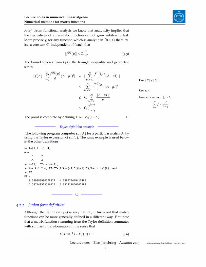
Proof. From functional analysis we know that analyticity implies thatthe derivatives of an analytic function cannot grow arbitrarily fast.More precisely, for any function which is analytic in D(µ, r) there ex-ists a constant Cr independent of i such that

∣ f (i)(µ)∣ ≤ Cri!ri . (4.5)

The bound follows from (4.5), the triangle inequality and geometricseries:

Use: ∥Bi∥ ≤ ∥B∥i .

Use: (4.5)

Geometric series: If ∣γ∣ < 1,

∞∑i=p

γi=

γp

1− γ.

∥ f (A)−N∑i=0

f (i)(µ)i!

(A − µI)i∥ = ∥∞

∑i=N+1

f (i)(µ)i!

(A − µI)i∥

≤∞

∑i=N+1

∣ f (i)(µ)∣i!

∥A − µI∥i

≤ Cr

∞

∑i=N+1

∥A − µI∥i

ri

≤ CrγN+1

1− γ

The proof is complete by defining C ∶= Crγ/(1− γ).

Taylor definition example

The following program computes sin(A) for a particular matrix A, byusing the Taylor expansion of sin(z). The same example is used belowin the other definitions.

>> A=[1,2; -5, 4]

A =

1 2

-5 4

>> m=21; FT=zeros(2);

>> for k=1:2:m; FT=FT+(A^k)*(-1)^((k-1)/2)/factorial(k); end

>> FT

FT =

8.339880980278327 -4.638979409410489

11.597448523526220 1.381411866162594

4.1.2 Jordan form definition

Although the definition (4.4) is very natural, it turns out that matrixfunctions can be more generally defined in a different way. First notethat a matrix function stemming from the Taylor definition commuteswith similarity transformation in the sense that

f (XBX−1) = X f (B)X−1 (4.6)


3



and it commutes with the diag operator in the sense that Definition of diag operator:

diag(F1, . . . , Fk) ∶=

⎡⎢⎢⎢⎢⎢⎣

F1⋱

Fk

⎤⎥⎥⎥⎥⎥⎦

In matlab, the corresponding commandis blkdiag.

f (diag(F1, . . . , Fk)) = diag( f (F1), . . . , f (Fk)), (4.7)

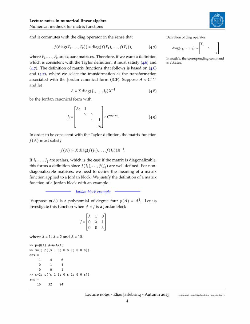
where F1, . . . , Fk are square matrices. Therefore, if we want a definitionwhich is consistent with the Taylor definition, it must satisfy (4.6) and(4.7). The definition of matrix functions that follows is based on (4.6)and (4.7), where we select the transformation as the transformationassociated with the Jordan canonical form (JCF). Suppose A ∈ Cn×n

and letA = X diag(J1, . . . , Jq)X−1 (4.8)

be the Jordan canonical form with

Ji =

⎡⎢⎢⎢⎢⎢⎢⎢⎢⎣

λi 1⋱ ⋱

⋱ 1λi

⎤⎥⎥⎥⎥⎥⎥⎥⎥⎦

∈ Cni×ni . (4.9)

In order to be consistent with the Taylor defintion, the matrix functionf (A) must satisfy

f (A) ∶= X diag( f (J1), . . . , f (Jq))X−1.

If J1, . . . , Jq are scalars, which is the case if the matrix is diagonalizable,this forms a definition since f (J1), . . . , f (Jq) are well defined. For non-diagonalizable matrices, we need to define the meaning of a matrixfunction applied to a Jordan block. We justify the definition of a matrixfunction of a Jordan block with an example.

Jordan block example

Suppose p(A) is a polynomial of degree four p(A) = A4. Let usinvestigate this function when A = J is a Jordan block

J =

⎡⎢⎢⎢⎢⎢⎢⎣

λ 1 00 λ 10 0 λ

⎤⎥⎥⎥⎥⎥⎥⎦

where λ = 1, λ = 2 and λ = 10.

>> p=@(A) A*A*A*A;

>> s=1; p([s 1 0; 0 s 1; 0 0 s])

ans =

1 4 6

0 1 4

0 0 1

>> s=2; p([s 1 0; 0 s 1; 0 0 s])

ans =

16 32 24


4



0 16 32

0 0 16

>> s=10; p([s 1 0; 0 s 1; 0 0 s])

ans =

10000 4000 600

0 10000 4000

0 0 10000

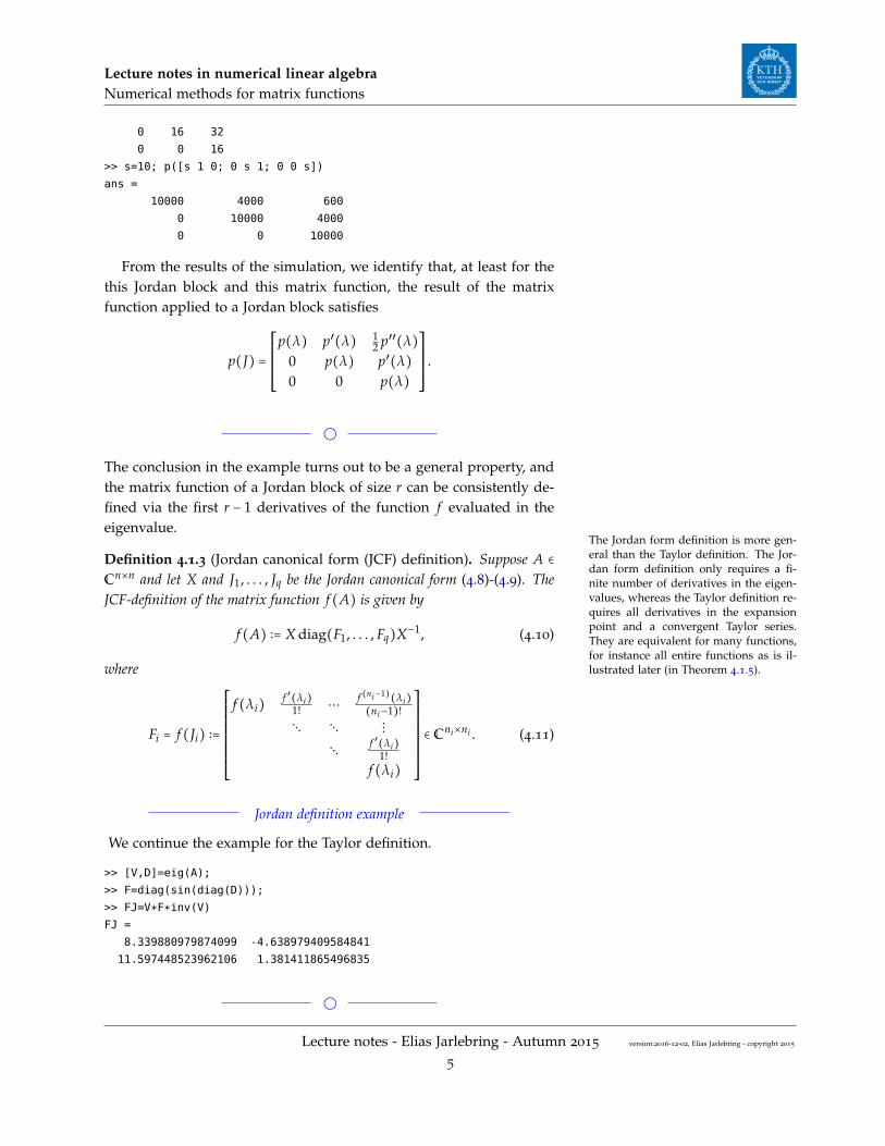
From the results of the simulation, we identify that, at least for thethis Jordan block and this matrix function, the result of the matrixfunction applied to a Jordan block satisfies

p(J) =

⎡⎢⎢⎢⎢⎢⎢⎣

p(λ) p′(λ) 12 p′′(λ)

0 p(λ) p′(λ)0 0 p(λ)

⎤⎥⎥⎥⎥⎥⎥⎦

.

The conclusion in the example turns out to be a general property, andthe matrix function of a Jordan block of size r can be consistently de-fined via the first r − 1 derivatives of the function f evaluated in theeigenvalue.

The Jordan form definition is more gen-eral than the Taylor definition. The Jor-dan form definition only requires a fi-nite number of derivatives in the eigen-values, whereas the Taylor definition re-quires all derivatives in the expansionpoint and a convergent Taylor series.They are equivalent for many functions,for instance all entire functions as is il-lustrated later (in Theorem 4.1.5).

Definition 4.1.3 (Jordan canonical form (JCF) definition). Suppose A ∈Cn×n and let X and J1, . . . , Jq be the Jordan canonical form (4.8)-(4.9). TheJCF-definition of the matrix function f (A) is given by

f (A) ∶= X diag(F1, . . . , Fq)X−1, (4.10)

where

Fi = f (Ji) ∶=

⎡⎢⎢⎢⎢⎢⎢⎢⎢⎢⎢⎣

f (λi)f ′(λi)

1! ⋯ f (ni−1)(λi)

(ni−1)!

⋱ ⋱ ⋮⋱ f ′(λi)

1!f (λi)

⎤⎥⎥⎥⎥⎥⎥⎥⎥⎥⎥⎦

∈ Cni×ni . (4.11)

Jordan definition example

We continue the example for the Taylor definition.

>> [V,D]=eig(A);

>> F=diag(sin(diag(D)));

>> FJ=V*F*inv(V)

FJ =

8.339880979874099 -4.638979409584841

11.597448523962106 1.381411865496835


5



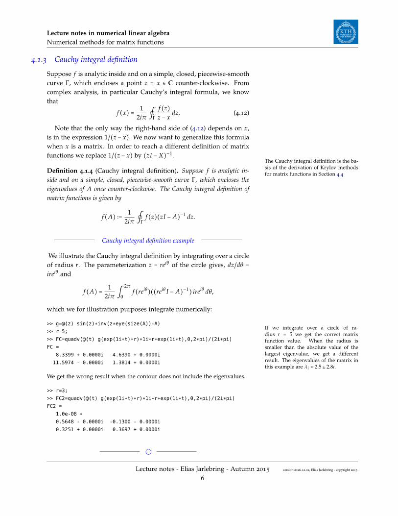
4.1.3 Cauchy integral definition

Suppose f is analytic inside and on a simple, closed, piecewise-smoothcurve Γ, which encloses a point z = x ∈ C counter-clockwise. Fromcomplex analysis, in particular Cauchy’s integral formula, we knowthat

f (x) = 12iπ ∮Γ

f (z)z − x

dz. (4.12)

Note that the only way the right-hand side of (4.12) depends on x,is in the expression 1/(z − x). We now want to generalize this formulawhen x is a matrix. In order to reach a different definition of matrixfunctions we replace 1/(z − x) by (zI −X)−1.

The Cauchy integral definition is the ba-sis of the derivation of Krylov methodsfor matrix functions in Section 4.4Definition 4.1.4 (Cauchy integral definition). Suppose f is analytic in-

side and on a simple, closed, piecewise-smooth curve Γ, which encloses theeigenvalues of A once counter-clockwise. The Cauchy integral definition ofmatrix functions is given by

f (A) ∶= 12iπ ∮Γ

f (z)(zI − A)−1 dz.

Cauchy integral definition example

We illustrate the Cauchy integral definition by integrating over a circleof radius r. The parameterization z = reiθ of the circle gives, dz/dθ =ireiθ and

f (A) = 12iπ ∫

2π

0f (reiθ)((reiθ I − A)−1) ireiθ dθ,

which we for illustration purposes integrate numerically:

If we integrate over a circle of ra-dius r = 5 we get the correct matrixfunction value. When the radius issmaller than the absolute value of thelargest eigenvalue, we get a differentresult. The eigenvalues of the matrix inthis example are λi ≈ 2.5± 2.8i.

>> g=@(z) sin(z)*inv(z*eye(size(A))-A)

>> r=5;

>> FC=quadv(@(t) g(exp(1i*t)*r)*1i*r*exp(1i*t),0,2*pi)/(2i*pi)

FC =

8.3399 + 0.0000i -4.6390 + 0.0000i

11.5974 - 0.0000i 1.3814 + 0.0000i

We get the wrong result when the contour does not include the eigenvalues.

>> r=3;

>> FC2=quadv(@(t) g(exp(1i*t)*r)*1i*r*exp(1i*t),0,2*pi)/(2i*pi)

FC2 =

1.0e-08 *0.5648 - 0.0000i -0.1300 - 0.0000i

0.3251 + 0.0000i 0.3697 + 0.0000i


6



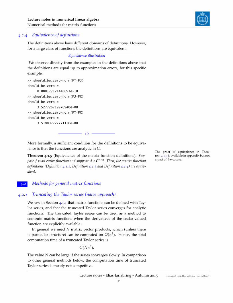
4.1.4 Equivalence of definitions

The definitions above have different domains of definitions. However,for a large class of functions the definitions are equivalent.

Equivalence illustration

We observe directly from the examples in the definitions above thatthe definitions are equal up to approximation errors, for this specificexample.

>> should_be_zero=norm(FT-FJ)

should_be_zero =

8.008177121446691e-10

>> should_be_zero=norm(FJ-FC)

should_be_zero =

3.527726719978948e-08

>> should_be_zero=norm(FT-FC)

should_be_zero =

3.519037727771136e-08

More formally, a sufficient condition for the definitions to be equiva-lence is that the functions are analytic in C.

The proof of equivalance in Theo-rem 4.1.5 is available in appendix but nota part of the course.

Theorem 4.1.5 (Equivalence of the matrix function definitions). Sup-pose f is an entire function and suppose A ∈ Cn×n. Then, the matrix functiondefinitions (Definition 4.1.1, Definition 4.1.3 and Definition 4.1.4) are equiv-alent.

x4.2 Methods for general matrix functions

4.2.1 Truncating the Taylor series (naive approach)

We saw in Section 4.1.1 that matrix functions can be defined with Tay-lor series, and that the truncated Taylor series converges for analyticfunctions. The truncated Taylor series can be used as a method tocompute matrix functions when the derivatives of the scalar-valuedfunction are explicitly available.

In general we need N matrix vector products, which (unless thereis particular structure) can be computed on O(n3). Hence, the totalcomputation time of a truncated Taylor series is

O(Nn3).

The value N can be large if the series converges slowly. In comparisonto other general methods below, the computation time of truncatedTaylor series is mostly not competitive.


7



4.2.2 Eigenvalue-eigenvector approach (naive approach)

If the matrix is diagonalizable, the Jordan form consists of diagonalelements, and the columns of X consists of the eigenvectors. Hence,the formula

f (A) = X diag( f (λ1), . . . , f (λn))X−1

gives a procedure to compute f (A) if we can compute X and λ1, . . . , λn.From previous parts of the course: Thestandard rough estimate for the compu-tation of the eigenpairs of a dense matrixwith a QR-method O(n3).

Under the assumption that computing all eigenpairs has compu-tational cost O(n3), an eigen-decomposition approach has computa-tional cost

O(n3).

For large-scale problems, the eigendecomposition approach is in gen-eral faster than the truncated Taylor series. However, we learned inother parts of this course that the Jordan canonical form is not numer-ically stable with respect to unstructured rounding errors. Very smallrounding errors can generate very large errors in the output. This isoften the case for non-symmetric matrices where the eigenvalues areclose to eachother. This can seriously jeopardize the reliability of themethod.

4.2.3 The Schur-Parlett method

An advanced version of the Schur-Parlett method is implemented in thematlab command funm.

The Schur form does not suffer from the same rounding errors disad-vantages as the Jordan form. For this reason, in the parts of the coursewhere we learned about eigenvalue computations, in particular whenwe learned the QR-method, we focused the Schur factorization, ratherthan a Jordan decomposition. The Schur-Parlett method is analogouslybased on the Schur factorization rather than the Jordan decomposition,which we used (for diagonalizable matrices) in Section 4.2.2.

Suppose A = Q∗TQ is a (complex) Schur factorization, where Q ∈Cn×n is an orthogonal matrix and T an upper triangular matrix. Fromthe fact that all definitions commute with similarity transformation(4.6) we can use that

f (A) = Q∗ f (T)Q. (4.13)

Hence, an approach based on the Schur factorization can be imple-mented in a straightforward way with (4.13) if we know how to com-pute the matrix function for the triangular matrix T. This can be doneas follows.

As a first step to a general method for triangular matrices, we de-rive an explicit formula for two-by-two triangular matrices. All of thematrix-function definitions satisfy

FT = TF (4.14)


8



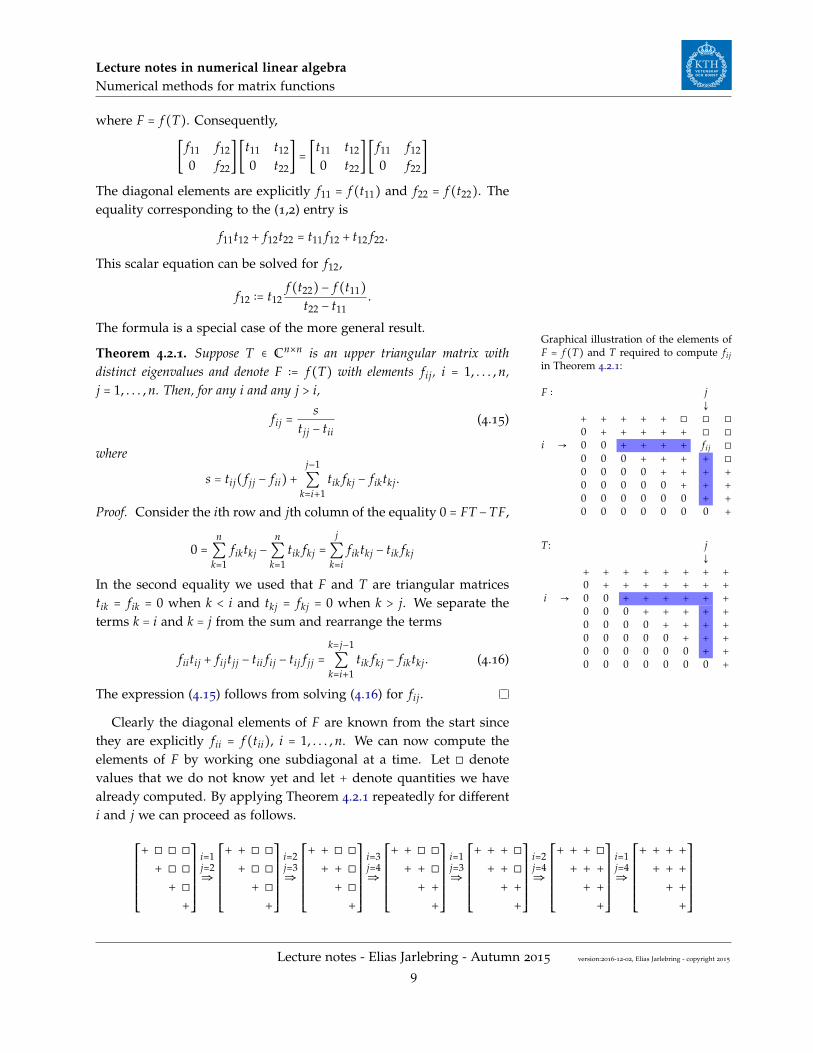
where F = f (T). Consequently,

[ f11 f12

0 f22] [t11 t12

0 t22] = [t11 t12

0 t22] [ f11 f12

0 f22]

The diagonal elements are explicitly f11 = f (t11) and f22 = f (t22). Theequality corresponding to the (1,2) entry is

f11t12 + f12t22 = t11 f12 + t12 f22.

This scalar equation can be solved for f12,

f12 ∶= t12f (t22)− f (t11)

t22 − t11.

The formula is a special case of the more general result.Graphical illustration of the elements ofF = f (T) and T required to compute fijin Theorem 4.2.1:

F ∶ j↓

+ + + + + ◻ ◻ ◻

0 + + + + + ◻ ◻

i → 0 0 + + + + fij ◻

0 0 0 + + + + ◻

0 0 0 0 + + + +

0 0 0 0 0 + + +

0 0 0 0 0 0 + +

0 0 0 0 0 0 0 +

T: j↓

+ + + + + + + +

0 + + + + + + +

i → 0 0 + + + + + +

0 0 0 + + + + +

0 0 0 0 + + + +

0 0 0 0 0 + + +

0 0 0 0 0 0 + +

0 0 0 0 0 0 0 +

Theorem 4.2.1. Suppose T ∈ Cn×n is an upper triangular matrix withdistinct eigenvalues and denote F ∶= f (T) with elements fij, i = 1, . . . , n,j = 1, . . . , n. Then, for any i and any j > i,

fij =s

tjj − tii(4.15)

where

s = tij( f jj − fii)+j−1

∑k=i+1

tik fkj − fiktkj.

Proof. Consider the ith row and jth column of the equality 0 = FT−TF,

0 =n∑k=1

fiktkj −n∑k=1

tik fkj =j

∑k=i

fiktkj − tik fkj

In the second equality we used that F and T are triangular matricestik = fik = 0 when k < i and tkj = fkj = 0 when k > j. We separate theterms k = i and k = j from the sum and rearrange the terms

fiitij + fijtjj − tii fij − tij f jj =k=j−1

∑k=i+1

tik fkj − fiktkj. (4.16)

The expression (4.15) follows from solving (4.16) for fij.

Clearly the diagonal elements of F are known from the start sincethey are explicitly fii = f (tii), i = 1, . . . , n. We can now compute theelements of F by working one subdiagonal at a time. Let ◻ denotevalues that we do not know yet and let + denote quantities we havealready computed. By applying Theorem 4.2.1 repeatedly for differenti and j we can proceed as follows.

⎡⎢⎢⎢⎢⎢⎢⎢⎢⎣

+ ◻ ◻ ◻+ ◻ ◻+ ◻+

⎤⎥⎥⎥⎥⎥⎥⎥⎥⎦

i=1j=2⇒

⎡⎢⎢⎢⎢⎢⎢⎢⎢⎣

+ + ◻ ◻+ ◻ ◻+ ◻+

⎤⎥⎥⎥⎥⎥⎥⎥⎥⎦

i=2j=3⇒

⎡⎢⎢⎢⎢⎢⎢⎢⎢⎣

+ + ◻ ◻+ + ◻+ ◻+

⎤⎥⎥⎥⎥⎥⎥⎥⎥⎦

i=3j=4⇒

⎡⎢⎢⎢⎢⎢⎢⎢⎢⎣

+ + ◻ ◻+ + ◻+ ++

⎤⎥⎥⎥⎥⎥⎥⎥⎥⎦

i=1j=3⇒

⎡⎢⎢⎢⎢⎢⎢⎢⎢⎣

+ + + ◻+ + ◻+ ++

⎤⎥⎥⎥⎥⎥⎥⎥⎥⎦

i=2j=4⇒

⎡⎢⎢⎢⎢⎢⎢⎢⎢⎣

+ + + ◻+ + ++ ++

⎤⎥⎥⎥⎥⎥⎥⎥⎥⎦

i=1j=4⇒

⎡⎢⎢⎢⎢⎢⎢⎢⎢⎣

+ + + ++ + ++ ++

⎤⎥⎥⎥⎥⎥⎥⎥⎥⎦


9



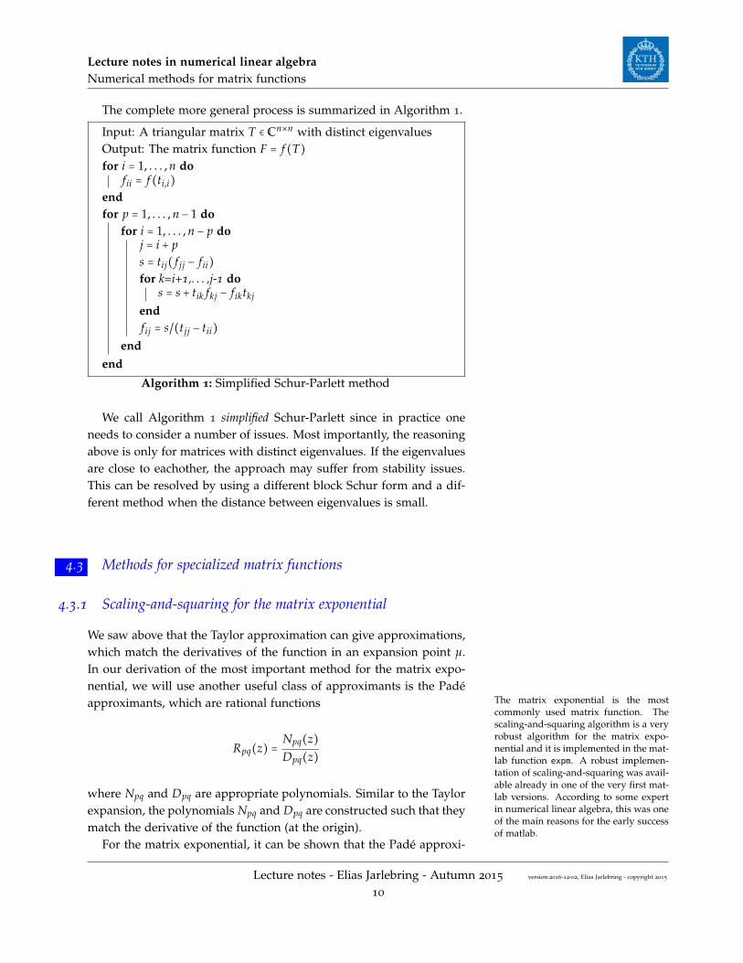
The complete more general process is summarized in Algorithm 1.

Input: A triangular matrix T ∈ Cn×n with distinct eigenvaluesOutput: The matrix function F = f (T)for i = 1, . . . , n do

fii = f (ti,i)endfor p = 1, . . . , n − 1 do

for i = 1, . . . , n − p doj = i + ps = tij( f jj − fii)for k=i+1,. . . ,j-1 do

s = s + tik fkj − fiktkj

endfij = s/(tjj − tii)

endend

Algorithm 1: Simplified Schur-Parlett method

We call Algorithm 1 simplified Schur-Parlett since in practice oneneeds to consider a number of issues. Most importantly, the reasoningabove is only for matrices with distinct eigenvalues. If the eigenvaluesare close to eachother, the approach may suffer from stability issues.This can be resolved by using a different block Schur form and a dif-ferent method when the distance between eigenvalues is small.

x4.3 Methods for specialized matrix functions

4.3.1 Scaling-and-squaring for the matrix exponential

We saw above that the Taylor approximation can give approximations,which match the derivatives of the function in an expansion point µ.In our derivation of the most important method for the matrix expo-nential, we will use another useful class of approximants is the Padéapproximants, which are rational functions

Rpq(z) =Npq(z)Dpq(z)

where Npq and Dpq are appropriate polynomials. Similar to the Taylorexpansion, the polynomials Npq and Dpq are constructed such that theymatch the derivative of the function (at the origin).

The matrix exponential is the mostcommonly used matrix function. Thescaling-and-squaring algorithm is a veryrobust algorithm for the matrix expo-nential and it is implemented in the mat-lab function expm. A robust implemen-tation of scaling-and-squaring was avail-able already in one of the very first mat-lab versions. According to some expertin numerical linear algebra, this was oneof the main reasons for the early successof matlab.

For the matrix exponential, it can be shown that the Padé approxi-


10



mants are

Npq(z) =p

∑k=0

(p + q − k)!p!(p + q)!k!(p − k)!

zk

Dpq(z) =q

∑k=0

(p + q − k)!q!(p + q)!k!(p − k)!

(−z)k.

These rational functions Rpq are constructed such that p+ q derivativesof Rpq match the derivatives of ez.

−3 −2 −1 0 1 2 30

5

10

15

20

25

z

y

ez

R11(z)R22(z)R33(z)

(a) Error in Padé approximation

0 0.1 0.2 0.3 0.4 0.5 0.6 0.7 0.8 0.910−1610−1410−1210−10

10−810−610−4

10−2100

α

Rel

ativ

eer

ror

p = q = 1p = q = 2p = q = 3p = q = 4

(b) ∥Rpq(αA)− exp(αA)∥/∥ exp(αA)∥

Figure 4.1: Illustration of the Padé ap-proximation for the matrix exponential.

This type of Padé approximants are only good approximations nearthe origin. They can be used to directly good approximations of thematrix exponential

exp(A) ≈ Rpq(A) = Dpq(A)−1Npq(A),

when ∥A∥ is small.The property (4.17) can be derived fromthe simple fact that

f (A)g(A) = h(A)

where h(z) = f (z)g(z).

It will in general not be a good approximation if ∥A∥ is large. For-tunately, this problem can be handled by exploiting the fact that

exp(A) = exp(A/m)m, (4.17)

for any m. In particular, we may scale A by m such that Rpq(A/m) is anaccurate approximation of exp(A/m). The approximation of exp(A),can subsequently be computed by forming Rpq(A/m)m. If m is a powerof two, m = 2j, then this last stage can be done very efficiently, with jmatrix-matrix multiplications.

Further details of the error analysis canbe found in references [4, Chapter 11.3]By further considerations of the approximant it can be shown that

if

∥A∥∞2j ≤ 1/2


11



then there exists E ∈ Rn×n such that

Fpq = eA+E (4.18)

AE = EA (4.19)

∥E∥∞ ≤ ε(p, q)∥A∥∞ (4.20)

ε(p, q) = 23−(p+q) p!q!(p + q)!(p + q + 1)!

(4.21)

By using these bounds we arrive at the main algorithm for the matrixexponential. The algorithm consists of first computing the rationalfunction and subsequently repeatedly squaring the result.

Input: δ > 0 and A ∈ Rn×n

Output: F = exp(A + E) where ∥E∥∞ ≤ δ∥A∥∞.begin

j = max(0, 1+floor(log2(∥A∥∞)))A = A/2j

Let q be the smallest non-negative integer such that ε(q, q) ≤ δ.D = I; N = I; X = I; c = 1for k = 1 ∶ q do

c = c(q − k + 1)/((2q − k + 1)k)X = AX; N = N + cX; D = D + (−1)kcX

endSolve DF = N for Ffor k = 1 ∶ j do

F = F2

endend

Algorithm 2: Scaling-and-squaring for the matrix exponential

4.3.2 Matrix square root

The matrix square root can be used tosolve partial-differential equations withcertain types of absorbing boundaryconditions. It has applications in for in-stance quantum physics (density func-tional theory) and it can be used to com-pute matrix logarithms and polar de-compositions.

We have now seen many examples of matrix functions which stem-ming from entire functions. The matrix square root is an importantexample of a function which is not analytic in the entire plane. In fact,it is usually defined by a system of equations rather than as an exten-sion of a scalar valued function. Any matrix X that satisfies X2 = Ais called a matrix square root of A. If A does not have any eigenval-ues in (−∞, 0] ⊂ C, there exists a specific matrix square root calledthe principal square root, which we can define with the definitionsabove as follows. Suppose F = f (A) is defined with Definition 4.1.3 forf (x) =

√x. Then,

F2 = X diag(F1, . . . , Fq)X−1X diag(F1, . . . , Fq)X−1 =X diag(F2

1 , . . . , F2q )X−1 = X diag(J1, . . . , Jq)X−1 = A,


12



since

F2i = Ji, i = 1, . . . , q.

For the scalar case, x =√

a is obviously a root to the nonlinear scalarequation g(x) = x2 − a = 0. Newton-Raphson’s method for g(x) is,xk+1 = xk − g(xk)/g′(xk) = xk − (x2

k − a)/2xk = xk/2+ a/2xk.The matrix function generalization is

Xk+1 =12(Xk +X−1

k A). (4.22)

Although the iteration (4.22) can be shown to be equivalent to New-ton’s method in matrix form and therefore exhibits local quadratic con-vergence in general, it is in a certain sense numerically unstable. Thiscan be explained by the fact that local convergence of (4.22) requirescommutativity of X0, X1, . . .. Due to round-off errors the commuta-tivity is not satisfied. Suppose we have an accurate approximation ofA1/2 such that Xk = A1/2 + ε∆, where ε will be thought of as a smallscalar parameter. Then,

The reasoning in (4.23) suggests at leastloss of quadratic convergence due toround-off errors, and justifies the badperformance of (4.22).

Xk+1 = 12(A1/2 + ε∆ + (A1/2 + ε∆)−1 A) (4.23a)

= A1/2 + ε

2(∆ − A−1/2∆A1/2)+O(ε2). (4.23b)

The term ∆ − A−1/2∆A1/2 vanishes if ∆ commutes with A, otherwise itwill in general not vanish.

If we want to use the Schur-Parlettmethod (in Section 4.2.3) to computethe principal matrix square root weneed to compute a Schur factorization ofA. The Denman-Beavers iteration (4.24)does not require a Schur factorization,but instead requires an inverse. In somesituations the inverse is easier to com-pute than the Schur factorization, for in-stance if A is tridiagonal.

Denman and Beavers proposed [3] an equivalent variant of (4.22)which does not exhibit the same sensitivity with respect to roundingerrors. The Denman-Beavers iteration is derived as follows. Due tothe fact that X0 = A, the matrices X0, X1, . . . commute. Hence, AX−1

k =A1/2X−1

k A1/2 and equation (4.22) can be rewritten as

Xk+1 =12(Xk + A1/2X−1

k A1/2).

By setting Yk = A−1/2Xk A−1/2, we have an iteration with two matrices

Xk+1 = 12(Xk +Y−1

k ) (4.24a)

Yk+1 = 12(Yk +X−1

k ) (4.24b)

with initial conditions X0 = A and Y0 = I. By construction, if Xk → A1/2,Yk → A−1/2.

It can be shown that this iteration is not as sensitive to roundingerrors. In contrast to (4.22) the convergence of the Denman-Beaversiteration (4.24) does not depend in the same way on commutativity.


13



4.3.3 Matrix sign function

In systems and control, the underlyingmethod to solve the Riccati equation isbased on the matrix sign function.

The (scalar-valued) sign function is for real numbers defined as

sign(a) =⎧⎪⎪⎨⎪⎪⎩

−1 a < 0

1 a > 0

and normally undefined for a = 0. The matrix sign function is anotherOne of the leading methods in quan-tum chemistry is derived from the ma-trix sign function.

matrix function which appears frequently in various fields. In order toconstruct a matrix function generalization, we first generalize the signto complex numbers. We here work only with the following propertywhich generalizes consistently to complex numbers,

sign(a) = ∣a∣a=

√a2

a.

We have in the previous section seen how to define the matrix squareroot, so we can in a consistent way generalize the matrix sign as follows

sign(A) ∶= A−1√

A2. (4.25)

The previous section directly also gives us an iterative approach for thematrix sign function, by first computing B = A2, C =

√B multiplying

by A−1C. However, rather than taking these separate steps it turnsout to be advantageous to integrate the operations of such a Newtonapproach (4.22) into a quite simple iteration. If we apply (4.22) tocompute the square root of the square, we have, X0 = A2 and

Xk+1 =12(Xk + A2X−1

k ) (4.26)

and sign(A) = A−1X∞. We now rephrase the iteration by defining

Sk = A−1Xk, (4.27)

such that sign(A) = S∞. Note that S0 = A−1X0 = A−1 A2 = A. More-over, after carrying out the substitution (4.27), (4.26) can be equivalentyphrased as

Sk+1 =12(Sk + S−1

k ). (4.28)

The iteration (4.28) is usually referred to as the Newton method formatrix sign function.

* Theorem of equivalence *It has global quadratic convergence in exact arithmetic, in the fol-

lowing sense.

Theorem 4.3.1 (Global quadratic convergence of (4.28)). Suppose A ∈Rn×n has no eigenvalues on the imaginary axis. Let S = sign(A), and Sk begenerated by (4.28). Let

Gk ∶= (Sk − S)(Sk + S)−1. (4.29)

Then,


14



• Sk = S(I +Gk)(I −Gk)−1 for all k,

• Gk → 0 as k →∞,

• Sk → S as k →∞, and

•∥Sk+1 − S∥ ≤ 1

2∥S−1

k ∥∥Sk − S∥2. (4.30)

Proof. From the fact that SkS = SSk and S2 = I, we have

(Sk ± S)2 = S2k ± 2SSk + I

= Sk(Sk + S−1k ± 2S)

= 2Sk(Sk+1 ± S) (4.31)

The inequality (4.30) follows by taking norms of (4.31) with the minussign. Now note that (4.31) imply that

If all eigenvalues of a matrix B are lessthan one in modulus, we have

∥Bm∥ = ∥V−1ΛmV∥ ≤ ∥V−1

∥∥V∥∥Λm∥→ 0

when m →∞.

Gk+1 = (Sk+1 − S)(Sk+1 + S)−1 =S−1

k (Sk − S)2(Sk + S)2Sk = (Sk − S)2(Sk + S)−2 = G2k (4.32)

such that Gk = G2k

0 . The eigenvalues of G0 are µ = (λ − sign(λ))/(λ +sign(λ)) such that ∣µ∣ < 1 and Gk → 0. Finally, the proof is completedby noting that

Sk = S(I +Gk)(I −Gk)−1.

The Riccati equation (4.33) is an impor-tant equation in systems and control, inparticular stochastic and optimal con-trol. Riccati equations can be solved withthe MATLAB command care.

Sign function and Riccati equation

An important application of matrix sign function is its use in a solu-tion method for quadratic matrix equation called the Riccati equation

G + ATX +XA −XFX = 0. (4.33)

It can be solved for X when F and G symmetric positive definite asThe matrix sign function approach isconsidered one of the leading numeri-cal methods for the Riccati equation. Aderivation of the formula in the examplecan be found in [2].

follows. For illustative purposes we computed the matrix sign withformula (4.25).

>> A=[2 1 ; 2 2]; F=[5 4; 4 6];G=[1 -1 ; -1 3];

>> K=[A’ G; F -A];

>> signm=@(X) inv(X)*sqrtm(X^2);

>> W2=signm(K)-eye(4);

>> [Q,R]=qr(W2(:,1:2));

>> X=-R\Q’*W2(:,3:4);

>> norm(G+A’*X+X*A-X*F*X)

ans =

4.2717e-15


15



x4.4 Krylov methods for f (A)bWe have above seen several methods to compute f (A) for specializedf as well as general situations. These methods are mostly suitable fordense matrices. We will now see a method which is suitable for largeand sparse problems. In many applications, it is sufficient to computethe action of the matrix function on a vector:

f (A)b (4.34)

where b ∈ Cn. The method we present next computes (4.34) directly,instead of first computing f (A) and then multiplying by b. It is basedon Arnoldi’s method and the only way A is accessed in the algorithmis via matrix-vector products.

4.4.1 Derivation of Arnoldi approximation of matrix functions

The Cauchy integral formula definition (Definition 4.1.4) can be com-bined with the quantity we want to compute (4.34) such that

f (A)b = −12iπ ∮Γ

f (z)((A − zI)−1b) dz. (4.35)

In the approach we take now, the shifted linear system of equations

x = (A − zI)−1b, (4.36)

in (4.35) is approximated by means of Krylov subspace approxima-tions.

Arnoldi decomposition for shifted linear systems

Our approximation of (4.36) is computed by applying Arnoldi’s methodto the shifted linear system. We first establish some properties ofArnoldi’s method when it is applied to a linear systems.

As we have seen earlier in the course, aKrylov subspace is defined by the spanof the iterates of the power method,

Km(A, b) ∶= span(b, Ab, . . . , Am−1b).

Due to the fact that the span is unchanged by adding or subtractingmultiples of the vectors, from the definition of a Krylov subspace onecan verify that

Km(A − σI, b) = Km(A, b).

This implies that the Krylov subspace is independent of shift. TheThe shift-invariance illustrated inLemma 4.4.1 shows that from theArnoldi decomposition of a matrix, wecan construct the Arnoldi decomposi-tion of the shifted matrix without anyadditional cost.

Arnoldi method is a procedure which generates an Arnoldi factoriza-tion,

AQm = QmHm+1,m + eTmqm+1hm+1,m, (4.37)

where the columns of Qm span the associated Krylov subspace. Theshift-invariance holds also for the Arnoldi factorization.

Lemma 4.4.1. Suppose Qm ∈ Cn×m, Hm ∈ C(m+1)×m is an Arnoldi factor-ization (4.37) associated with Km(A, b). Then, for any σ ∈ C, Qm ∈ Cn×m

Notational convenience in (4.38):

Im+1,m =

⎡⎢⎢⎢⎢⎢⎢⎢⎣

1⋱

10 ⋯ 0

⎤⎥⎥⎥⎥⎥⎥⎥⎦

∈ R(m+1)×m.


16



and Hm −σIm+1,m is an Arnoldi factorization associated with Km(A−σI, b),

(A − σI)Qm = Qm+1(Hm − σIm+1,m). (4.38)

Proof. The conclusion (4.38) follows from subtracting σQm from theArnoldi factorization AQm = Qm+1Hm = Qm Hm + hm+1,mqm+1eT

m.

Hence, the Arnoldi factorization associated with Km(A − σI, b) canbe easily reconstructed from the Arnoldi factorization associated withKm(A, b), by shifting the Hessenberg matrix Hm and using the samebasis matrix Qm.

FOM is an abbreviation for full orthogo-nalization method. The name was histori-cally given to distinguish it from other(now less used) methods based on in-complete orthogonalization in the un-derlying Gram-Schmidt process.

GMRES vs FOM: The approximation(4.39) corresponds to an element ofKm(A, b) such that the residual satis-fies QT

m(Ax − b) = 0, whereas the GM-RES approximation corresponds to anelement of Km(A, b) which minimizesminx∈Km(A,b) ∥Ax − b∥2 = ∥Ax − b∥2.

FOM for shifted linear system of equations

In the part in this course on sparse linear systems, we learned thatGMRES was a natural procedure to extract an approximation of a lin-ear system by means of minimizing the residual over approximationsin a Krylov subspace. For the purpose of approximating f (A)b, viaapproximation of (A − zI)−1b we will work with a slightly differentway to extract an approximation from the Krylov subspace, called theFOM-approximation.

We define the FOM-approximation of the linear system Ax = b by

x = Qm H−1m QT

mb = Qm H−1m e1∥b∥. (4.39)

This approximation can be derived by assuming that x ∈ Km(A, b) andimposing that the residual is orthogonal to the mth Krylov subspace,QT

m(Ax − b) = 0.Due to Lemma 4.4.1, the Krylov approximation of the shifted linear

system (A − σI)x = b is

x = Qm(Hm − σI)−1e1∥b∥. (4.40)

Note that this approximation can be computed for many σ by onlycomputing one Arnoldi factorization.

The Krylov approximation of a matrix function

By using the approximation stemming from FOM applied to a linearsystem expressed in (4.40) with the Cauchy integral formulation (4.35),we have

f (A)b ≈ −12iπ ∮Γ

f (z)Qm(Hm − zI)−1e1∥b∥ dz =

Qm1

2iπ ∮Γf (z)(zI − Hm)−1 dz(e1∥b∥) = Qm f (Hm)e1∥b∥.

This serves as a justification of our approximation scheme.

Definition 4.4.2 (Krylov approximation of a matrix function). Let Qm ∈Cn×m and Hm,m ∈ Cm×m correspond to an Arnoldi factorization (4.37) of the


17



matrix A with q1 = b/∥b∥. The Krylov approximation of a matrix function isdefined as

fm ∶= Qm f (Hm)e1∥b∥. (4.41)

Note that the Krylov approximation (4.41) also requires the evalu-ation of a matrix function. However, the Hessenberg matrix Hm is ingeneral much smaller than the original problem and computing f (Hm)is relatively inexpensive in comparison to carrying out the Arnoldimethod, at least if m ≪ n, which is typically the case for large andsparse problems.

Example

For many problems, the convergence is superlinear in practice. See thevideo demonstration

http://www.math.kth.se/~eliasj/krylov_matfun_approx.mp4

4.4.2 Convergence theory of Krylov approximation of matrix func-tions

Recall: A normal matrix is a matrix satis-fying AT A = AAT , which is the case forinstance if the matrix is symmetric. Notall normal matrices are symmetric matri-ces.

Similar to the Arnoldi method for eigenvalue problems and GMRES,the convergence can be characterized with a min-max expression. Toillustrate the convergence, we present only a result for normal matri-ces. Unlike the other min-max bounds in this course, the maximum isnot taken over a discrete set, but a continuous convex compact set Ωcontaining the eigenvalues of A.

The proof of Theorem 4.4.3 is beyondthe scope of the contents of the course.A proof can be found in [Error estima-tion and evaluation of matrix functions viathe Faber transform, Beckermann, Reichel,SIAM J. Numer. Anal., 47:3849-3883,2009]

Theorem 4.4.3. Suppose A ∈ Cn×n is a normal matrix and suppose Ω ⊂ C

is a convex compact set such that λ(A) ⊂ Ω. Let fm be the Krylov approxi-mation of f (A)b defined by (4.41). Then,

∥ f (A)b − fm∥ ≤ 2∥b∥ minp∈Pm−1

maxz∈Ω

∣ f (z)− p(z)∣.

Interpretation of bound

The bound gives several qualitative interpretations of the error. Suf-ficient conditions for fast convergence can be easily identified: Themethod will work well if

• f (z) can be well approximated with low-order polynomials

• λ(A) are clustered together such that Ω can be chosen small

Similar to other min-max bounds in this course, qualitative under-standing can be found by bounding using particular choices of the


18


http://www.math.kth.se/~eliasj/krylov_matfun_approx.mp4


polynomials. Let qm be the truncated Taylor expansion

qm(z) ∶=m∑i=0

f (m)(0)i!

zm.

Hence, rm(z) = f (z)− qm is the remainder term in the Taylor expansionof f . Suppose now that Ω is a subset of a disk of radius ρ centered atthe origin Ω ⊂ D(ρ, 0). Then

maxz∈Ω

rm(z) ∼ρm−1

(m − 1)!

and ∥ f (A)b − fm∥ ≤ em ∼ ρm−1

(m−1)! → 0 as m → ∞. This shows that themethod is convergent. The speed of convergence is usually muchfaster than what is predicted by this Taylor series bound.

4.4.3 Application of Krylov methods for exponential integrators

Typically, in our setting, (4.42) stemsfrom the discretization of a partial dif-ferential equation and n ≫ 1

The Krylov approximation techniques for matrix functions have turnedout to be useful in combination with techniques for differential equa-tions. We can use them to numerically compute solutions to the ordi-nary differential equation (ODE),

y′(t) = g(y(t)), y(0) = y0 (4.42)

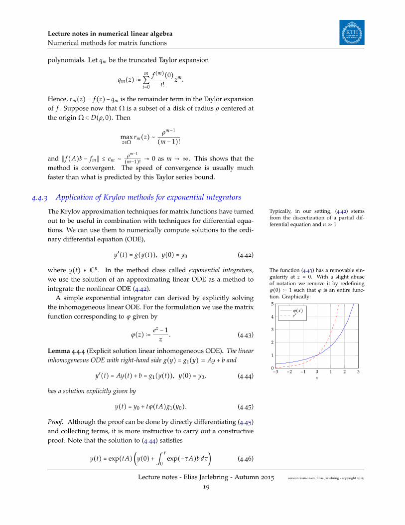
where y(t) ∈ Cn. In the method class called exponential integrators, The function (4.43) has a removable sin-gularity at z = 0. With a slight abuseof notation we remove it by redefiningϕ(0) ∶= 1 such that ϕ is an entire func-tion. Graphically:

−3 −2 −1 0 1 2 30

1

2

3

4

5

x

ϕ(x)ex

we use the solution of an approximating linear ODE as a method tointegrate the nonlinear ODE (4.42).

A simple exponential integrator can derived by explicitly solvingthe inhomogeneous linear ODE. For the formulation we use the matrixfunction corresponding to ϕ given by

ϕ(z) ∶= ez − 1z

. (4.43)

Lemma 4.4.4 (Explicit solution linear inhomogeneous ODE). The linearinhomogeneous ODE with right-hand side g(y) = g1(y) ∶= Ay + b and

y′(t) = Ay(t)+ b = g1(y(t)), y(0) = y0, (4.44)

has a solution explicitly given by

y(t) = y0 + tϕ(tA)g1(y0). (4.45)

Proof. Although the proof can be done by directly differentiating (4.45)and collecting terms, it is more instructive to carry out a constructiveproof. Note that the solution to (4.44) satisfies

y(t) = exp(tA) (y(0)+∫t

0exp(−τA)b dτ) (4.46)


19



From the Taylor definition of the matrix exponential we can integrateexplicitly,

∫t

0exp(−τA) dτ = −A−1(exp(−tA)− I)

such that (4.46) simplifies to

Use: A−1 exp(tA)A = exp(tA)y(t) = exp(tA)y(0)− exp(tA)A−1(exp(−tA)− I)b

= (y(0)+ A−1(exp(tA)− I)Ay(0))+ (A−1(exp(tA)− I)b)

= y(0)+ tϕ(tA)g1(y(0)), (4.47)

which proves (4.45).

The formula (4.45) is exact for the ODE (4.44), but in general notfor the nonlinear ODE (4.42). The simplest exponential integrator for(4.42) is based on applying (4.45) as a time-stepping method for (4.42).We approximate y1 ≈ y(h) by

y1 = y0 + hϕ(hA)g(y0) (4.48)

where A = g′(y0) is the Jacobian of g. The approximation techniquescan be repeated.

Definition 4.4.5 (Forward Euler exponential integrator). Let 0 = t0 <t1 < ⋯ < tN . The forward Euler exponential integrator associated with(4.45) for (4.42) generate the approximations yk ≈ y(tk), k =, . . . , N definedas

yk+1 = yk + hk ϕ(hk Ak)g(yk) (4.49)

where hk = tk+1 − tk and Ak ∶= g′(yk).

The method in Definition 4.4.5 is exact for the linear inhomogeneouscase (4.44), and one step can be proven to be second order in h in thegeneral case.

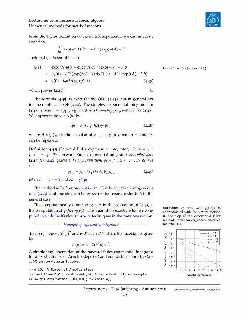
The computationally dominating part in the evaluation of (4.49) isthe computation of ϕ(hA)g(y0). This quantity is exactly what we com-puted in with the Krylov subspace techniques in the previous section.

Example of exponential integrator

Let f (y) = Ay + c(bTy)2 and y(0), b, c ∈ Rn. Then, the Jacobian is givenby

f ′(y) = A + 2(bTy)cbT .

A simple implementation of the forward Euler exponential integratorfor a fixed number of Arnoldi steps (m) and equidistant time-step (h =1/N) can be done as follows.

Illustration of how well ϕ(hA) f isapproximated with the Krylov methodin one step of the exponential Eulermethod. Faster convergence is observedfor smaller h.

0 2 4 6 8 10 12 14 16 18 2010−14

10−12

10−10

10−8

10−6

10−4

10−2

100

Arnoldi iteration m

Rel

ativ

eer

ror

inϕ(

hA)

f(y) h = 0.2

h = 0.1h = 0.05h = 0.02

>> m=20; % Number of Arnoldi steps

>> randn(’seed’,0); rand(’seed’,0); % reproducability of example

>> A=-gallery(’wathen’,100,100); n=length(A);


20



>> b=zeros(n,1); b(round(n/2))=1; b=sparse(b); c=b;

>> N=10; tv=linspace(0,1,N+1); h=tv(2)-tv(1);

>> J=@(y) A+2*(b’*y)*(c*b’);;

>> g=@(y) A*y+c*(b’*y)^2;

>> y0=eye(n,1); y=y0;

>> for k=1:N

>> v=g(y);

>> [Q,H]=arnoldi(J(y),v,m);

>> phig=Q(:,1:m)*(varphi(h*H(1:m,1:m))*eye(m,1));

>> y=y+h*phig*norm(v);

>> end

>> sol=ode45(@(t,v) g(v), [0,1],y0,’RelTol’,1e-10);

>> rel_err=norm(sol.y(:,end)-y)/norm(y)

rel_err =

2.9768e-06

A more thorough convergence analysis (beyond the scope of thiscourse) shows that the error behaves as

∥ϕ(tA)b − fm∥ = O(tm) (4.50)

As we have seen above, designing an exponential integrator requiresthe choice of many quantities. In particular, the choice of step-lengthis inherently very difficult. We have the trade-offs in order obtain fastconvergence and accurate results. We want

• small h, because it leads to fast convergence in the Krylov methodas is illustrated in (4.50);

• small h, because it leads to smaller discretization error as the dis-cretization error (per step) is quadratic in h; but

• large h, because then we can complete the integration in N ∼ 1/hsteps.

The typical approach to balance these quantities often involves problem-specific a posteriori error analysis of the Krylov method as well as theintegrator.

x4.5 Further reading and literature

The most complete source of information for matrix functions is theworks of Nick Higham, in particular his monograph [5] but also sum-mary papers such as [6]. The work of Horn and Johnson [9] containsa thorough and more theoretical approach to matrix functions. Ma-trix functions also appear in concise formats in standard literature inmatrix computations [4, 1]. The presentation of the matrix square root


21



in Secion 4.3.2 was inspired by sections from [1] and [5], whereas thescaling-and-squaring in Section 4.3.1 was based on [4]. Further in-formation about Section 4.4.3 can be found in [8, 7] and referencestherein. The topic of matrix functions is a very active topic. There isactive research on rational Krylov methods for matrix functions, con-ditioning numbers and development of new methods for other matrixfunctions. Considerable research is carried out on convergence of itera-tive methods for matrix functions and also specialized preconditioningtechniques.

x4.6 Appendix - Omitted proofs

Proof of Theorem 4.1.5. First note that all three definitions satisfy (4.6)and (4.7). If we select X and B as the Jordan canonical form of A, wehave

fT(A) = fT(XBX−1) = X diag( fT(J1), . . . , fT(Ji))X−1

f J(A) = f J(XBX−1) = X diag( f J(J1), . . . , f J(Ji))X−1

fC(A) = fC(XBX−1) = X diag( fC(J1), . . . , fC(Ji))X−1.

Hence, the definitions are equivalent if and only if fT(J) = f J(J) =fC(J) for any Jordan block J = Ji. Therefore, it is sufficient to proveequivalence for an arbitrary Jordan block J ∈ Cm×m.

Definition 4.1.1⇔ Definition 4.1.3. We first show the result for mono-mials pk(z) ∶= zk. By induction we see that p(`)k (z) = `p(`−1)

k−1 (z) +zp(`)k−1(z) for any ` and k. By again using induction we have that

(J − µI)k = pk(J − µI) =

⎡⎢⎢⎢⎢⎢⎢⎢⎢⎢⎢⎣

pk(λ − µ) p′k(λ−µ)1! ⋯ p(m−1)

k (λ−µ)

(m−1)!

⋱ ⋱ ⋮⋱ p′k(λ−µ)

1!pk(λ − µ)

⎤⎥⎥⎥⎥⎥⎥⎥⎥⎥⎥⎦

.

(4.51)The function is analytic, so we can directly differentiate the Taylorexpansion j times

f (j)(λ) =∞

∑`=0

f (`)(µ)`!

p(j)` (λ − µ). (4.52)

We now combine (4.51) and (4.52) in the Taylor definition (4.4) to


22



establish the conclusion

fT(J) =∞

∑`=0

f (`)(µ)`!

(J − µI)` =

∞

∑`=0

f (`)(µ)`!

⎡⎢⎢⎢⎢⎢⎢⎢⎢⎢⎢⎣

p`(λ − µ) p′`(λ−µ)1! ⋯ p(m−1)

`(λ−µ)

(m−1)!

⋱ ⋱ ⋮⋱ p′`(λ−µ)

1!p`(λ − µ)

⎤⎥⎥⎥⎥⎥⎥⎥⎥⎥⎥⎦

=

⎡⎢⎢⎢⎢⎢⎢⎢⎢⎢⎢⎣

f (λ) f ′(λ)1! ⋯ f (m−1)

(λ)(m−1)!

⋱ ⋱ ⋮⋱ f ′(λ)

1!f (λ)

⎤⎥⎥⎥⎥⎥⎥⎥⎥⎥⎥⎦

.

The implication holds in both direction since the definitions areunique.

Definition 4.1.3⇔ Definition 4.1.4. It is easy to verify that that theexpression involving an inverse in the Cauchy integral formula isexplicitly

(zI − J)−1 =

⎡⎢⎢⎢⎢⎢⎢⎢⎢⎣

1/(z − λ) 1/(z − λ)2 ⋯ 1/(z − λ)m

⋱ ⋱ ⋮⋱ 1/(z − λ)2

1/(z − λ)

⎤⎥⎥⎥⎥⎥⎥⎥⎥⎦

(4.53)

Now let

F ∶= 12iπ ∮Γ

f (z)(zI − J)−1 dz.

From the (scalar) Cauchy integral formula and (4.53) we have

Fi,j =1

2iπ ∮Γ

f (z)(z − λ)j dz =

f (j−i)(λ)(j − i)!

, i = 1, . . . , m, j = i, . . . , m,

which coincides with the JCF-definition (4.11)

x4.7 Exercises matrix functions

1. Show that (4.6) is satisfied when f (A) is defined with (4.4).

2. Suppose Aα = B + αC and ∥B∥ = ∥C∥ = 1. Give a sufficient conditionon α ∈ R such that the Taylor definition provides a well-definedmatrix function f (Aα) when f (s) = sin(1/(s− 1)) for all µ ∈ (−∞, 0).


23



3. Let

A =

⎡⎢⎢⎢⎢⎢⎢⎢⎢⎣

α 1⋱ ⋱

⋱ 1α

⎤⎥⎥⎥⎥⎥⎥⎥⎥⎦

∈ Rn×n, b =

⎡⎢⎢⎢⎢⎢⎢⎣

1⋮1

⎤⎥⎥⎥⎥⎥⎥⎦

∈ Rn

and suppose f is an entire function. Determine a closed expressionfor

limn→∞

eT1 f (A)b.

using any matrix function definition.

4. Derive a constant c independent of t and A such that

exp(tA) ≤ c exp(t∥A∥)

for all t ∈ (0,∞).

5. Show that the there are at most 2n matrices F ∈ Cn×n which satisfy

F2 = A.

6. Show that f (A) f (B) = f (AB) if AB = BA for any definition.

7. Derive a Newton-algorithm for the kth matrix root. Show that localconvergence is sensitive to round-off errors.

8. In what sense is (4.28) related to (4.22)?

9. Generalize the Denman-Beavers iteration kth root.

10. Recall thatexp(A/2)2 = exp(A)

Now approximate A∆ = ∆A,

(exp(A/2)+∆0)2 = exp(A)+ 2∆0 exp(A/2)+∆20

((exp(A/4)+∆1)2 +∆0)2 = exp(A)+ 2∆0 exp(A/2)+∆20

11. Derive constants X, Y ∈ Rn×p and α such that

f (tA) = XYT f (αt)

when A = uvT for given u, v ∈ Rn. Use any matrix function defini-tion.

12. What is a ϕ-function?

13. Give an example of an exponential integrator.

14. Derive a matrix-function solution to the ODE y′(t) = Ax + b.


24



x4.8 Bibliography

[1] Å. Björck. Numerical methods in matrix computations. Springer, 2015.

[2] R. Byers. Solving the algebraic Riccati equation with the matrixsign function. Linear Algebra Appl., 85:267–279, 1987.

[3] E. Denman and A. N. Beavers. The matrix sign function and com-putations in systems. Appl. Math. Comput., 2:63–94, 1976.

[4] G. Golub and C. Van Loan. Matrix Computations. The Johns Hop-kins University Press, 2013. 4th edition.

[5] N. J. Higham. Functions of Matrices. Theory and Computation. SIAM,2008.

[6] N. J. Higham and A. H. Al-Mohy. Computing matrix functions.Acta Numerica, 19:159–208, 2010.

[7] M. Hochbruck, C. Lubich, and H. Selhofer. Exponential integratorsfor large systems of differential equations. SIAM J. Sci. Comput.,19(5):1552–1574, 1998.

[8] M. Hochbruck and A. Ostermann. Exponential integrators. ActaNumerica, 19:209–286, 2010.

[9] R. Horn and C. Johnson. Matrix analysis. Cambridge UniversityPress, New York, 1985.


25


numerical methods for matrix functions · numerical methods for matrix functions which is analytic...

Documents