numerical methods for pricing exotic options - imperial college
TRANSCRIPT
Numerical Methods for Pricing Exotic
Options
Dimitra Bampou
Supervisor: Dr. Daniel Kuhn Second Marker: Professor Berç Rustem
18 June 2008

2 Numerical Methods for Pricing Exotic Options
3 0BAbstract
Abstract
Derivative securities, when used correctly, can help investors increase their expected returns and minimize their exposure to risk. Options offer leverage and insurance for risk-averse investors. For the more risky investors, they can be ways of speculation. When an option is issued, we face the problem of determining the price of a product which depends on the performance of another security and on the same time we must make sure to eliminate arbitrage opportunities.
Due to the nature of those contracts, over the past decades a lot of research has focused on finding accurate valuation models for options. Popular pricing methods such as Black-Scholes PDE have proven to be inefficient for pricing exotic options as it is impossible to express their price in an analytic solution
In this project, we investigate two recently proposed valuation techniques. They approach the problem of pricing an option by approximating upper and lower bounds for the option price using semidefinite programming. We will explore the price dynamics of options and the efficiency of these methods for pricing European and Exotic options.
www.doc.ic.ac.uk/~db04/project/

4 Numerical Methods for Pricing Exotic Options

5 1BAcknowledgements
Acknowledgements
I would like to thank my supervisor, Dr. Daniel Kuhn, for his constant guidance and support during the project. His motivation and enthusiasm helped me develop a great interest in optimization and operations research.
I would like to acknowledge Professor Berç Rustem, my second marker, for his constructive comments and suggestions.
I would also like to thank my parents for being my inspiration. Finally I would like to thank my sister Elina and my friend George for their support all those years in London.
6 Numerical Methods for Pricing Exotic Options
Table of Contents
ABSTRACT 3
ACKNOWLEDGEMENTS 5
TABLE OF CONTENTS 6
INTRODUCTION 9
1.1 Motivation 9
1.2 Contributions 11
BACKGROUND 12
2.1 Linear and Semi-definite Programming 12
2.2 Probability and Measure Theory 13
2.3 The problem of Moments and Optimization with Polynomials 18
2.4 Mathematical Models for Asset Prices 20
2.5 Financial Background 23 2.5.1 Options 23 2.5.2 Role of Options 26
BLACK-SCHOLES AND MONTE CARLO METHODS 29
3.1 Black-Scholes 29
3.2 Monte Carlo Method 31 3.2.1 Geometric Brownian motion 31 3.2.2 Ornstein-Uhlenbeck process 32 3.2.3 Monte Carlo method for European Options 32 3.2.4 Monte Carlo for Asian options 32 3.2.5 Monte Carlo for Barrier options 33
BOUNDING OPTION PRICES BY SEMI DEFINITE PROGRAMMING 34
4.1 Formulation of the problem for a European Call option 34 4.1.1 Dual upper bound problem conversion to SDP 39 4.1.2 Dual lower bound problem conversion to SDP 40
4.2 Formulating the SDP for European Put options 42 4.2.1 Dual upper bound problem conversion to SDP 43
7 2BTable of Contents
4.2.2 Dual lower bound problem conversion to SDP 45
4.3 Calculating the moments 46
4.4 Conclusions 47
PRICING A CLASS OF EXOTIC OPTIONS VIA MOMENTS AND SDP RELAXATIONS 48
5.1 Formulating the problem 48
5.2 Asian Options 54 5.2.1 Formulation 54 5.2.2 Computing the moments of U 55
5.3 European Options 57 5.3.1 Formulation 57 5.3.2 Computing the moments of U 59
5.4 Barrier Options 60 5.4.1 Formulation 60 5.4.2 Defining the moments 63
NUMERICAL RESULTS 65
6.1 Software and Hardware 65
6.2 Pricing a Class of Exotic Options via Moments and SDP relaxations 65 6.2.1 European Call options 65 6.2.2 Asian Call Options 71
6.3 Bounding Option Prices by Semidefinite Programming 78
CONCLUSION 82
7.1 Qualitative Evaluation 82
7.2 Future Work 83
REFERENCES 84

8 Numerical Methods for Pricing Exotic Options
9 3BIntroduction
Chapter 1
Introduction
1.1 Motivation
An option, put in simple terms, is a contract between two parties, giving one of the parties the right but not the obligation to purchase or to sell an asset in the future. For example, given a stock selling at £50 today, A and B agree that in one year from now, B will have the option to purchase that stock from A for £54 for exchange of a fee. B pays the fee to A today and on the expiration date, B will exercise his right only if the stock is selling on the stock markets at a higher price. This type of option is called a European Call option.
The existence of options traces back thousands of years, in the Phoenicians and Ancient Greek civilizations. According to Aristotle (Luenberger 1998), Thales the Milesian, believed by observing the stars, that the olive harvest would be really good in the summer, so he rented in advance olive presses at a low price since demand was low during the winter. In the summer, his judgement was proved correct and by controlling the supply of the equipment while demand was high, he made profit.
Nowadays, options are considered to be extremely popular financial instruments as investors find them a really attractive way of investing their money. Options are usually included in portfolios as ways of hedging and speculation. For example, an investor believing that the stock price of IBM will rise, will enter a contract such as the one described above, making profit by selling the stock after the expiration of the option, if of course his judgment is proved to be correct. Options can also result in spectacular losses. The IBM stock price may not rise after all and the investor will lose the fee he paid for the option.
There are many standard types of options selling in the global financial markets, such as Europeans and Americans. Further, new types of options arise as investors try to create their preferred risk return profile for their portfolios. A special case of options called exotics has gain popularity. Each option is characterized by the way its payoff depends on price of the underlying asset.
The main challenge regarding the options market is how to price them fairly to avoid arbitrage opportunities. Regarding the above example, what is the optimal price that A should charge B today for the option he is selling? Certainly, B would
10 Numerical Methods for Pricing Exotic Options
not pay the same price for a similar option as the above with an exercise price of £70 instead of £54.
Perhaps the most popular valuation model for options is the Black-Scholes PDE, proposed by Robert C. Merton. The model is based on the theory that markets are arbitrage free and assumes that the price of the underlying asset is characterized by a Geometric Brownian motion (an Ito process). This method is commonly used for pricing European options as there is an analytic solution for their price. On the other hand, in most cases it is almost impossible to express the Black-Scholes PDE in an analytic formula that would calculate the prices of exotic options.
Another technique for pricing options is the binomial lattice model. In essence, it is a simplification of the Black-Scholes method as it considers the fluctuation of the price of the underlying asset in discrete time. Binomial lattices are easily implemented but can be computationally demanding. This model is typically used to determine the price of European and American options.
Monte Carlo simulation is a numerical method for pricing options. It assumes that in order to value an option, we need to find the expected value of the price of the underlying asset on the expiration date. Since the price is a random variable, one possible way of finding its expected value is by simulation. A disadvantage of this method is that it can be computationally demanding and to obtain an accurate result for the price of a simple Vanilla option, one would need to generate 105 random numbers. On the other hand, this model can be adapted to price almost any type of option.
In 2000, Bertsimas and Popescu proposed a semi definite programming approach for pricing European options. The method was later modified by Gotoh and Konno, who also proposed a cutting plane algorithm for solving the problem (Gotoh and Konno 2002). The objective of the method is to approximate upper and lower bounds, producing a tight set of possible values, for the price of a European option, given the first few moments of the risk neutral distribution of the price of the underlying asset, which can be modeled by any process (as long as we are able to calculate its moments). This is an advantage since market has shown that stock prices often do not behave as Geometric Brownian motion.
Recently, Lasserre, Prieto-Rumeau and Zervos introduced a new technique for pricing exotic options (Lasserre, Prieto-Rumeau and Zervos 2006). Their technique is based on the work of Dawson which involves the use of moments to derive a solution for martingale problems. According to this method, one needs to write the problem of finding the price of an option as an infinite system of 1st degree polynomials, whose variables are moments of certain measures. Thus one obtains a linear programming problem which cannot be solved because it is infinite. The objective is now to convert the above problem into a semidefinite
11 3BIntroduction
programming problem by applying finite dimensional relaxations to the moments of the above measures, thus creating moment and localizing matrices, which is a technique introduced by Lasserre in 2001. The advantage of this technique against the Black-Scholes model is that the distribution of the underlying asset can be modeled by many types of processes. Indeed in their paper, the authors have applied their method on European, Asian and Barrier options whose underlying asset can follow the GBM, the Ornstein-Uhlenbeck process or the standard square root process.
1.2 Contributions
The key contributions of the project are:
• We investigate two recently proposed methods for pricing options. The comparative advantage of these methods against traditional pricing techniques such as Monte Carlo is that they try to approximate upper and lower bounds for the prices of the options by finding appropriate measures for the prices of the underlying assets and formulating problems involving some moments of those measures (chapters 4, 5).
• We investigate the problem of moments, where we are interested in finding the maximum/minimum point of a non-convex polynomial. The solution of this problem lies on the fact that by requiring certain necessary and sufficient moment conditions, we can convert it into a convex problem (chapter 2).
• We analyze the method proposed by Gotoh and Konno for pricing European call options and we show how we can adapt it in order to find upper and lower bounds for the prices of put options (chapter 4).
• We consider the method proposed by Lasserre, Prieto-Rumeau and Zervos for pricing Asian and Barrier options using the problem of moments. We present the adaptation for pricing European options (chapter 5).
• We study several fundamental pricing techniques and we explore the dynamics of asset prices in the financial world (chapters 2, 3).
• We provide implementations of the above techniques in Matlab and we analyze the results. We then investigate the advantages and disadvantages for these techniques based on assumptions they rely on, their complexity and how easily can be adapted for other options (chapters 6, 7.1).
12 Numerical Methods for Pricing Exotic Options
Chapter 2
Background
In this chapter, we explain the mathematical concepts and the financial theory and calculus needed in order to understand the methods for derivative pricing described in this report. We focus on semidefinite programming, probability and measure theory and stochastic differential equations. We then apply these concepts in the financial world. We assume no prior knowledge of finance.
2.1 Linear and Semi-definite Programming
Linear programming (LP) is a technique used in optimization problems where the decision variables are linearly related. Linear programming is applied in decision making problems including the fields of engineering and finance. An LP problem consists of the decision variables, whose optimal values are what we need to approximate subject to some restrictions, referred to as constraints. The standard LP problem is defined as
0 , R ; R
R
In this problem, defined as the primal, we are interested in finding the optimal value of such that our objective function is minimized. The feasible region, the convex hull, of variable is defined by the constraints and 0. An LP problem can be solved using the SIMPLEX algorithm, which walks along the edges of the polyhedron defined by the constraints and finds the optimal solution.
We define the dual of the above is the dual variable, as problem, where
0 ; ,

13 4BBackground
The solution of the dual is bounded from above by the primal solution, , and the main duality theory states that given a pair of primal and dual problems, if one of them has an optimal solution, so does the other, and the optimal value of the objective functions are the same, .
A semi-definite programming problem (SDP) is an extension of a linear problem where the objective function is linear but the set of constraints is defined as a combination of positive semidefinite matrices. SDP are convex optimization problems since the constraints form a convex set and the objective is a linear (hence convex) function. To define the SPD problem formally, consider the set of symmetric matrices and , 0, … . Our decision variable is . Then an SDP is defined as
0
The constraints of an SDP define a convex cone of positive semidefinite matrices in the set of symmetric matrices. The main difference between an LP and a SDP is that a SDP is not a linear problem. SDP has a wide area of application and in this report we will focus on its use as a solution of polynomial optimization problems.
The dual of an SDP, with du f d as al variable is de ine
Y Y
0
The solution of the dual SDP problem is again bounded from above by the primal solution if both the primal and the dual have feasible solutions. Equality of the optimal primal and optimal dual solution holds if both are strictly feasible, i.e. if and ∑ are positive definite matrices.
SDP problems can be solved using interior point methods and many open source solvers exist such as Sedumi and SDPA.
2.2 Probability and Measure Theory
Given a set and a collection of subsets of then is algebra of subsets of if
i) ii) If then the complement of , , which means is closed
under complementation
14 Numerical Methods for Pricing Exotic Options
iii) For any , , which means that is closed under finite union. Hence is closed under finite intersection since and by ii
Additionally given , , … if th is called σ-al b . en ge ra
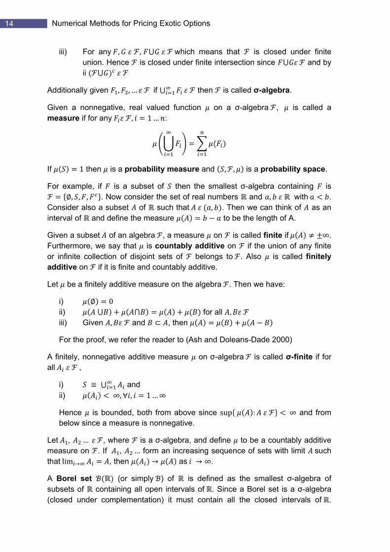
Given a nonnegative, real valued function on a σ-algebra , is called a measure if for any , 1… :
If 1 then is a probability measure and , , is a probability space.
For example, if is a subset of then the smallest σ-algebra containing is , , , . Now consider the set of real numbers and , with .
Consider also a subset of such that , . Then we can think of as an interval of and define the measure t be the length of o A.
Given a subset of an algebra , a measure on is called finite if ∞. Furthermore, we say that is countably additive on if the union of any finite or infinite collection of disjoint sets of belongs to . Also is called finitely additive on if it is finite and countably additive.
Let be a ditive measure on the algebra . Then we have: finitely ad
i) ii)
0 for all ,
iii) Given , and , then
For the proof, we refer the reader to (Ash and Doleans-Dade 2000)
A finitely, nonnegative additive measure on σ-algebra is called σ-finite if for all ,
i) and ii) ∞, , 1…∞
Hence is bounded, both from above since sup : ∞ and from measu is nonnegative. below since a re
Let , … , where is a σ-algebra, and define to be a countably additive measure on . If , … form an increasing sequence of sets with limit such that lim then ∞. , as
A Borel set (or simply ) of is defined as the smallest σ-algebra of subsets of containing all open intervals of . Since a Borel set is a σ-algebra (closed under complementation) it must contain all the closed intervals of .
15 4BBackground
Hence a Borel set contains all intervals of . Every subset of , i.e. any real number, belongs in the Borel set. One can think of a Borel set by starting with an interval on the set of real functions and add to the collection all the unions, intersections and complements of all th added in the le sets col ection.
Given a function : and a set , we define . Then is called Borel if : .
A Lebesgue-Stieltjes measure on is the measure on such that ∞ for each bounded interval (Ash and Doleans-Dade 2000). For a
distribution function : is increasing, i.e. and right continuous, i.e.lim . Then we have , 0. If is a decreasing sequence of points then , 0.
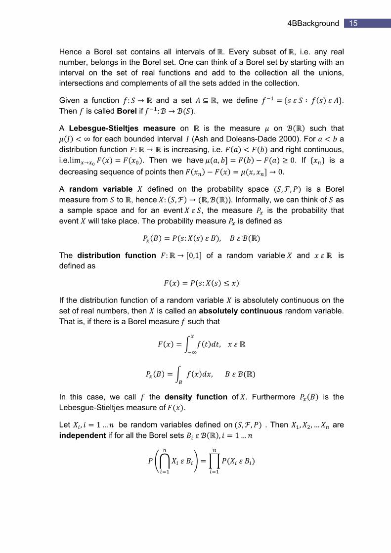
A random variable defined on the probability space , , is a Borel measure from to , hence : , , ). Informally, we can think of as a sample space and for an event , the measure is the probability that event will take place. T r ed as he p obability measure is defin
: ,
The distribution function : 0,1 of a random variable and is defined as
:
If the distribution function of a random variable is absolutely continuous on the set of real numbers, then is called an absolutely continuous random variable. That is, if there is a Borel measure such that
,
,
In this case, we call the density function of . Furthermore is the Lebesgue-Stieltjes measure of .
Let , 1… be random variables defined on , , . Then , , … are independent if for all the Borel sets , 1…

16 Numerical Methods for Pricing Exotic Options
If , 1… are independent random variables as defined above and ,1… is the distribution function of each , then the distribution function of the random variable is defined by
Define a set and a subset of . Then the indicator : 0,1 of is defined by
1, 0,
We define the expectation of a random variable defined on the probability space , , by
The moment about the mean, often referred to as the central moment is defined as . For 0, the 0-moment of a random variable is equal to 1. For 1, then the 1 moment is the expectation as defined above. We refer to the 2 central t , i.e. moment as he variance of
,
If , 1… are independent random variables defined on , , then
…
When more than one random variable is related with an experiment, we need to refer to random vectors. An dimentional random vector defined on the probability space , , is a Borel measure from to . Hence : and each random variable is a Borel measure. Now the probability measure is defined as
, :
The distribution function : 0,1 or equivalently the joint distribution function of a rand vom ector is given by
∞, : , 1… .

17 4BBackground
For an absolutely continuous random vector there is a Borel measure , which is the density function, such that
,
,
The covariance of tw as o random variables and is defined
,
From the above, we can see than | , |
The correlation coefficient of two rando s and is defined as m variable
,,
If and are independent then , 0 hence , 0. When they are completely dependent then , , 1.
Given a stochastic process, i.e. a sequence of random variables , ,… defined on the probability space , , , being a σ-algebra and , being sub σ-algebras of where each is measurable on respectively, we say that , ,… is a martingale relative to if the conditional expected value of given all , is qu e c u , that is e al to th expe ted val e of
| | ∞,| , 1,2, …
Let , be a martingale and be an increasing sequence of σ-algebras of . A random variable 1,2, … . ∞ is called a stopping time relative to if . A stopping time is a condition of whether to stop or continue a process.
Let be the first time that a 6 appears when we roll a fair die and be the number of 6’s appeared until the th roll. We can define to be a stopping time such that
6, 6,
18 Numerical Methods for Pricing Exotic Options
2.3 The problem of Moments and Optimization with Polynomials
The general problem of moments is defined as the problem where we want to derive the existence of a measure given some of its moments. In this section we give an introduction of the general problem of moments applied in finding extreme points of a non-convex polynomial and demonstrate how we can convert it into semi definite optimization problem through relaxations. We focus our analysis in unconstrained optimization problems of polynomials. For more details, we refer the reader to (J. B. Lasserre 2001). This section of the background is necessary in order to understand the method for pricing exotics in Chapter 5.
Given a multiindex we define the moment of order of a Borel measure on as
The of m s of measure up to order is given by . sequence oment
Let and to be the set of all Borel measures with finite moments of all orders supported on .
Given a real valued polynomial : we are interested in solving the problem
The polynomial , where | cannot be written as a sum of squares. Let be of degree . Hence we can write
, … ,
The b t oasis of he p lynomial is given by
1, … , , , , … , ,, , ,
The terms are the coefficient vectors of .
, … , … , , … , , …
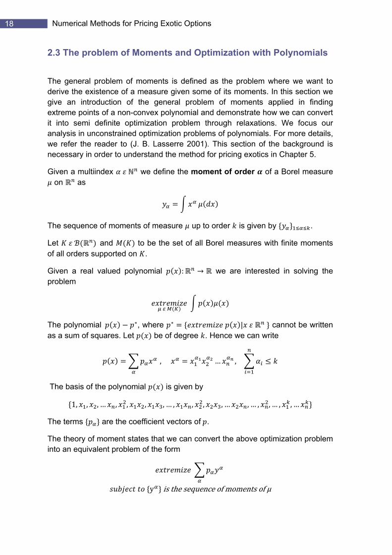
The theory of moment states that we can convert the above optimization problem into an equivalent problem of the form
y is the sequence of moments of µ
19 4BBackground
In order to express the constraint in mathematical terms, we need to introduce the concepts of moment and localizing matrices.
According to (J. B. Lasserre 2001), given a sequence yα , we introduce the sequence , , which is obtained by ordering the sequence with the same indices as the basis of the polynomial given above. For instance, when 2 and a 2 we h ve
0,y10,y01,y20,y11,y02,y30,y21,…,y04… y0
The moment matrix of is defined as
1, , 1 , 1… 1 1, yα, 1 y , yα β
β
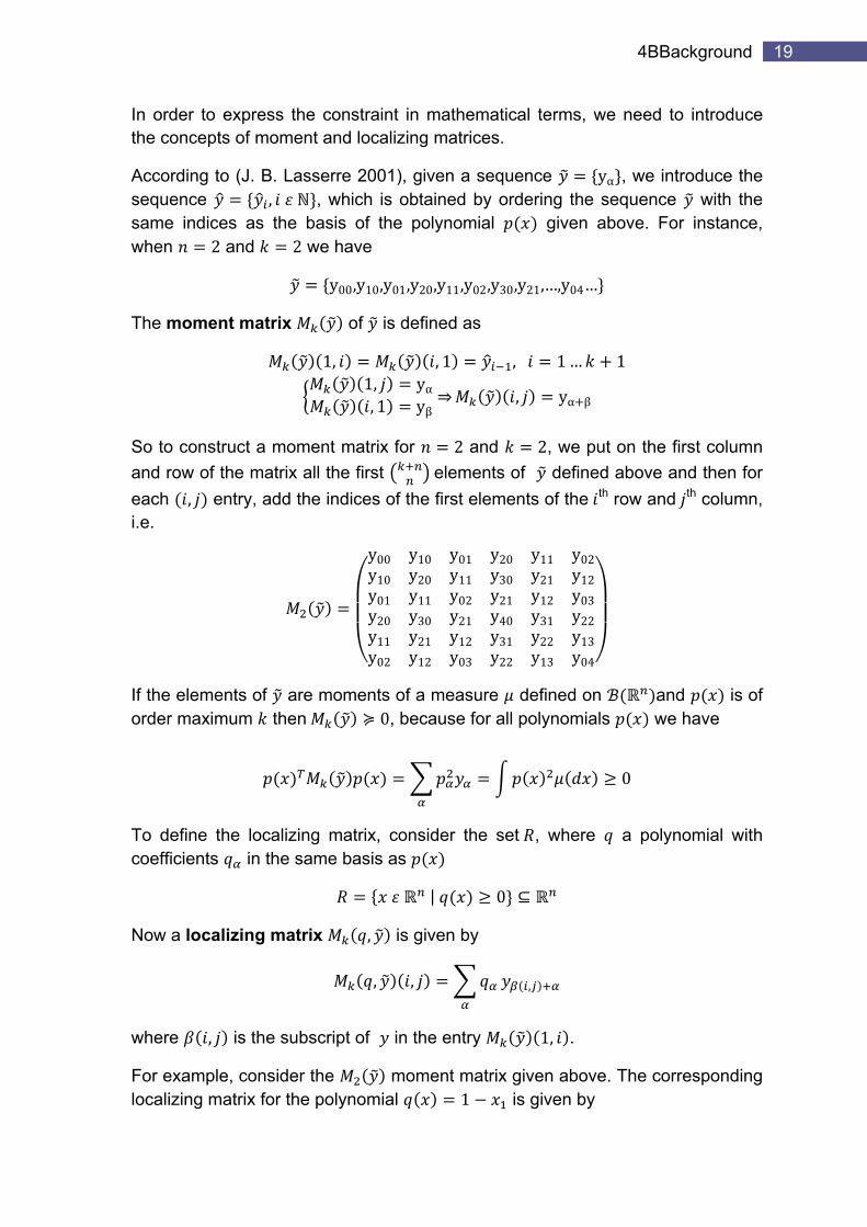
So to construct a moment matrix for 2 and 2, we put on the first column and row of the matrix all the first elements of defined above and then for each , entry, add the indices of the first elements of the th row and th column, i.e.
y00 y10 y01 y20 y11 y02y10 y20 y11 y30 y21 y12y01 y11 y02 y21 y12 y03y20 y30 y21 y40 y31 y22y11 y21 y12 y31 y22 y13y02 y12 y03 y2 y13 y042
If the elements of are moments of a measure defined on and is of order maximum then 0, because for all polynomials we have
0
To define the localizing matrix, consider the set , where a polynomial with coefficients in the same basis as
| 0
Now a localizing matrix , is given by
, , ,
where , is the subscrip o in the entry 1, . t f
For example, consider the moment matrix given above. The corresponding localizing matrix for the polynomial 1 is given by
20 Numerical Methods for Pricing Exotic Options
,
y00 y10 y10 y20 y01 y11 y20 y30 y11 y21 y02 y!2y10 y10 y20 y30 y11 y21 y30 y40 y21 y31 y12 y22y01 y10 y11 y21 y02 y12 y21 y31 y12 y22 y03 y13y20 y30 y30 y40 y21 y31 y40 y50 y31 y41 y22 y32y11 y21 y21 y31 y12 y22 y31 y41 y22 y32 y13 y23y02 y12 y12 y22 y03 y13 y22 y32 y13 y 3 y04 142 y
If the elements of are moments of a measure defined on and is of order maximum th we have en , 0, because for all polynomials
0 ,
The conditions , 0 and 0 are necessary but not sufficient, meaning that even if both matrices are positive semidefinite at the solution, may not be the sequence of moments of .
Returning now to the original problem, if we know that 0, then for polynomials , , 1, … . , 1… . we can write
Hence we can convert the original problem to a semi definite optimization problem
0 , 0
2.4 Mathematical Models for Asset Prices
Given an index set , a stochastic process is a sequence of random variables defined on a probability space , , . Thinking the index set as time, we
can model the price of a security using stochastic processes. We will start our discussion by taking the time as a discrete parameter followed by continuous time and derive 3 pricing models.
Random Walks are special random functions of time (Luenberger 1998). Suppose we have a time period 0, and this period is divided into intervals . Then a Random Walk is defined as
21 4BBackground
0√
~ 0,1
The standardized normal random variables are mutually uncorrelated, meaning 0, . Furthermore, for any we have
√
This difference is a le with the i res opertierandom variab nte ting pr s
i) For any , variables and are lmutually uncorre ated
ii) ∑ √ 0
iii) ∑ √ ∑
Random Walks are a discrete time process since time is divided into discrete time intervals. A Weiner process is a continuous time process, derived by taking the limit of a Random Walk as 0
√
Then a Weiner process is a process which satisfies the following properties:
i) ii) 0
~ 0, ,
iii) For any , variables and are mutually uncorrelated
An Ito process is a stochas d ich takes the form tic ifferential equation wh
, ,
The functions , and , are called the expected drift rate and the variance rate respectively and is a Weiner process.
22 Numerical Methods for Pricing Exotic Options
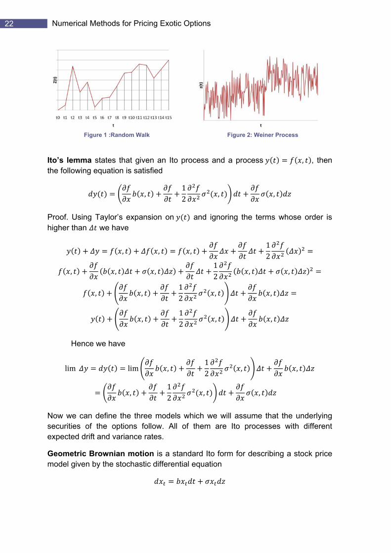
Figure 1 :Random Walk
Figure 2: Weiner Process
Ito’s lemma states that given an Ito process and a process , , then the following equation satisfied is
,1
, , 2
Proof. Using Taylor’s expansion on and ignoring the terms whose order is higher than we have
, , ,12
, , ,12 , ,
, ,12 , ,
,12 , ,
Hence we have
lim lim ,12 , ,
,12 , ,
Now we can define the three models which we will assume that the underlying securities of the options follow. All of them are Ito processes with different expected drift and variance rates.
Geometric Brownian motion is a standard Ito form for describing a stock price model given by the stochastic d e qiff rential e uation
23 4BBackground
The Ornstein-Uhlenbeck process which is used to model the price dynamics of interest rates is defined as
The Cox-Ingersoll-Ross interest rate model is n the following SDE give by
It is a one factor model (one source of market risk). The factor ensures mean reversion of interest rates towards the expected value with rate of adjustment . ensures that is always positive.
The mean reverting property of stochastic processes is a tendency experienced by some processes to return over time to their long run expected value. For example, interest rates and implied latility exhibit this property.vo
The infinitesimal generator of an n-dimentional Ito processes is an operator acting on the set of functions : , which are twice differentiable, have continuous e ond d e fo o ing l it xis s fo all s c erivatives and th ll w im e t r
lim f x12 f x
2.5 Financial Background
In this section we explain the notions of derivative securities related to this project, focusing on their payoff structures and their role in the financial system.
A derivative is a contract, a security, whose payoff depends on the value of some other security, called the underlying asset. The underlying asset can be a stock, a currency or a tangible asset such as corn. Options are derivative securities giving one of the parties “special rights”, depending on the nature of the option. We refer to the writer as the party who is selling the option and the holder as the one who is purchasing the option. The price paid by the holder to the writer in exchange for those “special rights” is called the premium.
2.5.1 Options The basic types of options are the European Call and Put options. A European Call option gives its holder the right, but not the obligation, to purchase from the writer a prescribed asset for a prescribed price at a prescribed time in the future (Higham 2004). On the other hand, a European Put option gives its holder the right, but not the obligation, to sell to the writer a prescribed asset for a prescribed price at a prescribed time in the future (Higham 2004). Suppose we have an underlying asset currently trading at , where are the days elapsed since the issue of the option. The maturity date of the option, i.e. the date which the holder of the option has the right to exercise the option, is . The price of the
24 Numerical Methods for Pricing Exotic Options
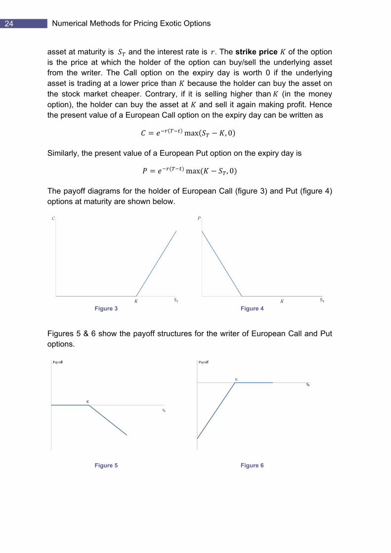
asset at maturity is and the interest rate is . The strike price of the option is the price at which the holder of the option can buy/sell the underlying asset from the writer. The Call option on the expiry day is worth 0 if the underlying asset is trading at a lower price than because the holder can buy the asset on the stock market cheaper. Contrary, if it is selling higher than (in the money option), the holder can buy the asset at and sell it again making profit. Hence the present value of a Euro ry day can be written as pean Call option on the expi
max , 0
Similarly, the present value o n the expiry day is of a European Put opti n o
max , 0
The payoff diagrams for the holder of European Call (figure 3) and Put (figure 4) options at maturity are shown below.
Figure 3
Figure 4
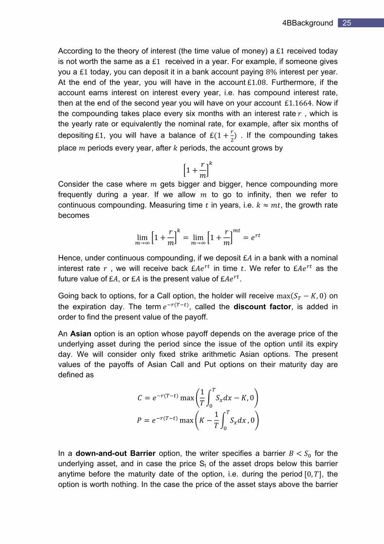
Figures 5 & 6 show the payoff structures for the writer of European Call and Put options.
Figure 5
Figure 6
25 4BBackground
According to the theory of interest (the time value of money) a £1 received today is not worth the same as a £1 received in a year. For example, if someone gives you a £1 today, you can deposit it in a bank account paying 8% interest per year. At the end of the year, you will have in the account £1.08. Furthermore, if the account earns interest on interest every year, i.e. has compound interest rate, then at the end of the second year you will have on your account £1.1664. Now if the compounding takes place every six months with an interest rate , which is the yearly rate or equivalently the nominal rate, for example, after six months of depositing £1, you will have a balance of £ 1 . If the compounding takes place periods every year, after periods, the account grows by
1
Consider the case where gets bigger and bigger, hence compounding more frequently during a year. If we allow to go to infinity, then we refer to continuous compounding. Measuring time in years, i.e. , the growth rate becomes
lim 1 lim 1
Hence, under continuous compounding, if we deposit £ in a bank with a nominal interest rate , we will receive back £ in time . We refer to £ as the future value of £ , or £ is the present value of £ .
Going back to options, for a Call option, the holder will receive max , 0 on the expiration day. The term , called the discount factor, is added in order to find the present value of the payoff.
An Asian option is an option whose payoff depends on the average price of the underlying asset during the period since the issue of the option until its expiry day. We will consider only fixed strike arithmetic Asian options. The present values of the payoffs of Asian Call and Put options on their maturity day are defined as
max1
, 0
max1
, 0
In a down-and-out Barrier option, the writer specifies a barrier for the underlying asset, and in case the price St of the asset drops below this barrier anytime before the maturity date of the option, i.e. during the period 0, , the option is worth nothing. In the case the price of the asset stays above the barrier
26 Numerical Methods for Pricing Exotic Options
throughout the duration of the option, the option has a payoff structure similar to a European option. Thus, the present values of the payoffs of down-and-out Barrier Call and Put options on the maturity day are defined as
0, , 0 max , 0 , , 0
0, , 0 max , 0 , , 0
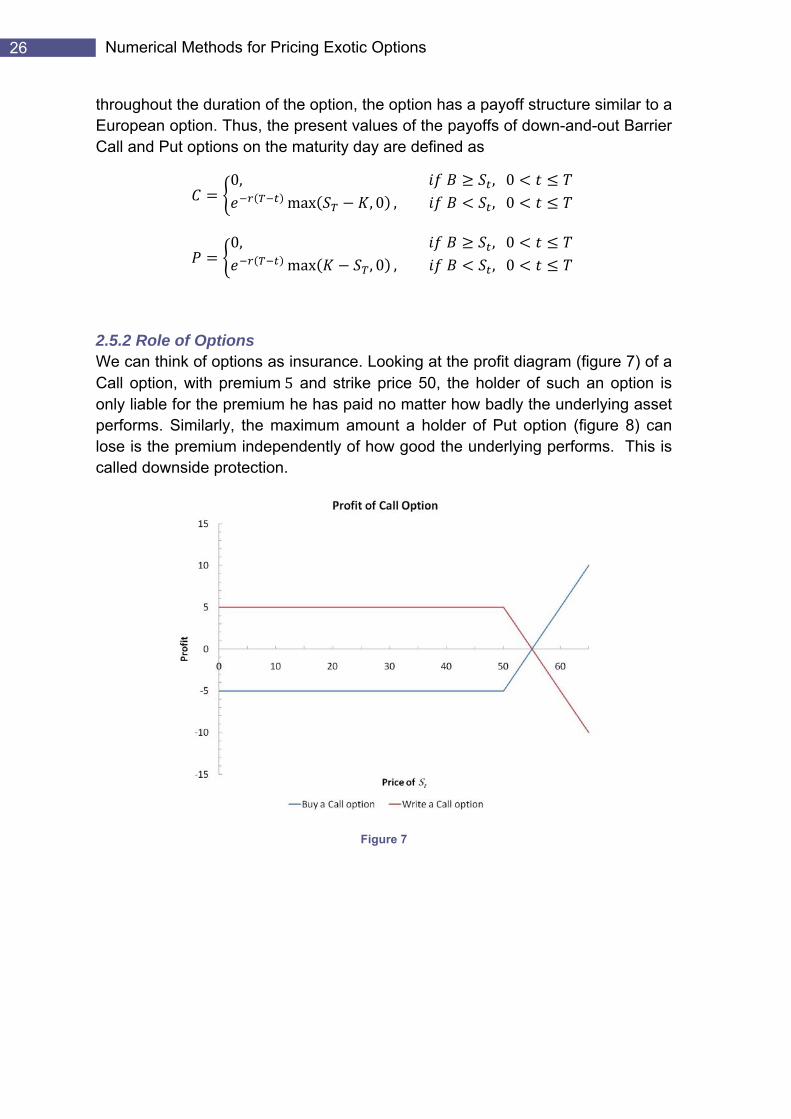
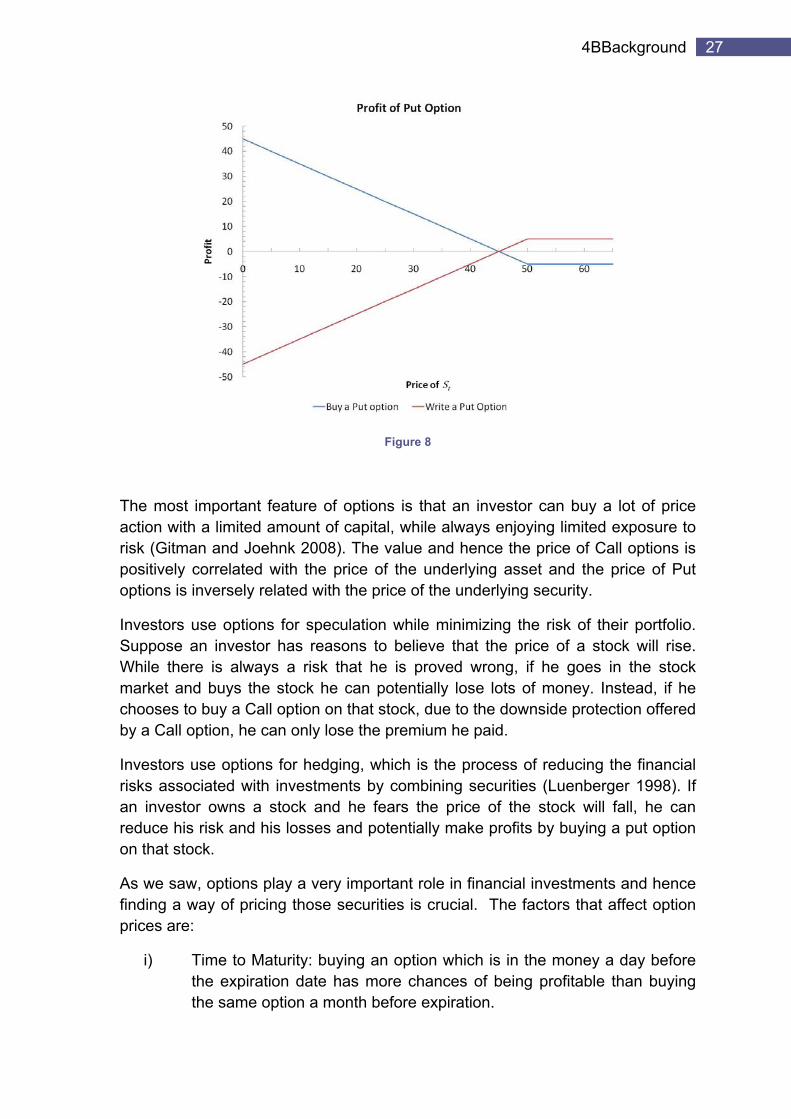
2.5.2 Role of Options We can think of options as insurance. Looking at the profit diagram (figure 7) of a Call option, with premium 5 and strike price 50, the holder of such an option is only liable for the premium he has paid no matter how badly the underlying asset performs. Similarly, the maximum amount a holder of Put option (figure 8) can lose is the premium independently of how good the underlying performs. This is called downside protection.
Figure 7
27 4BBackground
Figure 8
The most important feature of options is that an investor can buy a lot of price action with a limited amount of capital, while always enjoying limited exposure to risk (Gitman and Joehnk 2008). The value and hence the price of Call options is positively correlated with the price of the underlying asset and the price of Put options is inversely related with the price of the underlying security.
Investors use options for speculation while minimizing the risk of their portfolio. Suppose an investor has reasons to believe that the price of a stock will rise. While there is always a risk that he is proved wrong, if he goes in the stock market and buys the stock he can potentially lose lots of money. Instead, if he chooses to buy a Call option on that stock, due to the downside protection offered by a Call option, he can only lose the premium he paid.
Investors use options for hedging, which is the process of reducing the financial risks associated with investments by combining securities (Luenberger 1998). If an investor owns a stock and he fears the price of the stock will fall, he can reduce his risk and his losses and potentially make profits by buying a put option on that stock.
As we saw, options play a very important role in financial investments and hence finding a way of pricing those securities is crucial. The factors that affect option prices are:
i) Time to Maturity: buying an option which is in the money a day before the expiration date has more chances of being profitable than buying the same option a month before expiration.
28 Numerical Methods for Pricing Exotic Options
ii) Price movements of the underlying security: as the price of a stock rises, the Call option gains in value. A Call option, whose underlying asset is falling, is losing value.
iii) Price volatility of the underlying security: the more volatile the price of the underlying security, the greater the risk of an option being out of money.
iv) Interest rates: as we discussed, the present value of a cash flow depends on the level of interest rates.
Hence, option pricing models need to take into account those factors. Due to the importance of options, a lot of research is focused on finding the most accurate models. Monte Carlo simulations can be potentially applied to any type of option to determine an average price but the variance of the result is usually high, due to the probabilistic nature of the error estimates. There are techniques for variance reduction such as control variant which are out of the scope of this project. Instead, researchers are interested in deriving more accurate models each one reflecting the properties of each type of option.
29 5BBlack-Scholes and Monte Carlo Methods
Chapter 3
Black-Scholes and Monte Carlo Methods
In this chapter we give the details of some standard methods for pricing European and exotic options. We present the Black-Scholes PDE and explain how we adapt Monte Carlo simulations to price exotics.
3.1 Black-Scholes
Robert C. Merton proposed a mathematical model for pricing stock options in 1973. This model was named Black-Scholes (BS). Black-Scholes PDE is a method for pricing options in which the underlying stock is priced using the Black-Scholes model. The Black Scholes formula is the formula for pricing European Call and Put options using the Black-Scholes PDE. The BS model is based on the assumption that the stock price follows a Brownian motion, using the risk neutral probability.
The Black-Scholes equation tries to estimate the price of the underlying security of an option as an Ito process. To do that, we construct a portfolio with two products that try to replicate the current behavior of the derivate. The portfolio consists of a risk-free asset, for example a Bond, of value at time and interest rate such that and a stock whose price follows a geometric Brownian motion
Then the payoff function , of the derivative with the underlying security being the stock and measured at time must satisfy the following partial differential equation:
12
Proof. Applying Ito’s mma o we have le n
12 (3.1)
The portfolio that replicates the a unction at time is given by derivative p yoff f
30 Numerical Methods for Pricing Exotic Options
The coefficients and are selected in such a way so that replicates , . The instantaneous change in the value of the portfolio is thus
(3.2)
Since replicates , , the coefficients of and in (3.1) and (3.2) must be equal, hence
1
,
R
eplacing an in (3.2) and using the fact that ,
12
12
1,
12
The problem with the Black-Scholes PDE is that it is almost impossible to express it in an analytic formula, especially for exotic options. Furthermore, Black-Scholes PDE model works when we are pricing a security under risk neutrality. The theory states that and an investor regards an investment with rate of return and a risky investment with expected rate of return as equally attractive (Higham 2004).
The cumulative function of a standard normal distribution is given by
1√2
, ∞ 0, ∞ 1, 112
The analytic solution of the Black-Scholes PDE where we take , , , i.e. the payoff of a European Call option with strike price and exercise date is
31 5BBlack-Scholes and Monte Carlo Methods
,
ln 2√√
The pricing formula for a European put option uses and as defined above and is given by
,
3.2 Monte Carlo Method
The Monte Carlo is a famous algorithm for pricing European as well as exotic options hence it is used widely in the financial industry. Before we get into the details of the method, we need to find the analytic solutions of the stochastic differential equations of the Geometric Brownian motion and the Ornstein-Uhlenbeck process.
3.2.1 Geometric Brownian motion Suppose is the price of an asset at time and is the risk free interest rate. follows a Geometric Brownian ti tochastic differential equation mo on given by the s
We apply Ito’s lemma ng the oc . Then usi pr ess ln
12
ln12
ln12
12
Since is a Weiner process, we have √
with ~ 0,1 . Hence
√ Using the central limit theorem we see that is normally distributed with mean
and variance √ .
32 Numerical Methods for Pricing Exotic Options
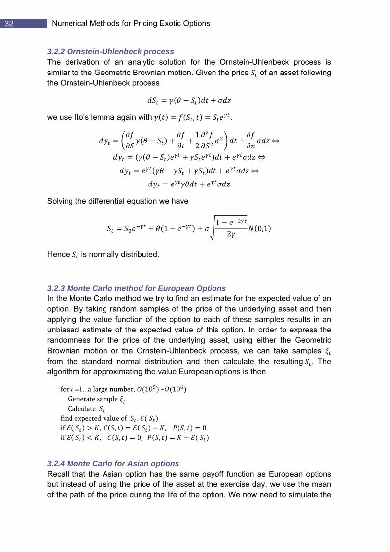
3.2.2 Ornstein-Uhlenbeck process The derivation of an analytic solution for the Ornstein-Uhlenbeck process is similar to the Geometric Brownian motion. Given the price of an asset following the Ornstein-Uhlenbeck process
we use Ito’s lemma again with , .
12
Solving the differential equation we have
11
2 0,1
Hence is normally distributed.
3.2.3 Monte Carlo method for European Options In the Monte Carlo method we try to find an estimate for the expected value of an option. By taking random samples of the price of the underlying asset and then applying the value function of the option to each of these samples results in an unbiased estimate of the expected value of this option. In order to express the randomness for the price of the underlying asset, using either the Geometric Brownian motion or the Ornstein-Uhlenbeck process, we can take samples from the standard normal distribution and then calculate the resulting . The algorithm for approximatin ropean options is then g the value Eu
for =1...a large number, 10 ~ 10 Generate sample l Calcu ate
if fin ed exp cted value of ,
, , , , 0 if , , 0, ,
3.2.4 Monte Carlo for Asian options Recall that the Asian option has the same payoff function as European options but instead of using the price of the asset at the exercise day, we use the mean of the path of the price during the life of the option. We now need to simulate the

33 5BBlack-Scholes and Monte Carlo Methods
price of the underlying asset to find its expected value and repeat this experiment 10 ~ 10 times in order to find a good approximation for the value of an
Asian option. Hence the drawback of this method is that it is extremely computationally demanding thus inefficient.
for =1...a large number, 10 ~ 10 for j=1...a large number, 10 ~ 10 Generate sample Calculate x e find e pect d value of ,
if fin ed exp cted value of all ,
, , , , 0 if , , 0, ,
3.2.5 Monte Carlo for B r optionsa rier The algorithm is similar to the one used for pricing Asian options. We need to add a constraint such that if , where is the barrier, the option is worth nothing. Here is an outline for the a t lgori hm
for =1...a large number, 10 ~ 10 for j=1...a large number, 10 ~ 10 Generate sample Calculate
d m nim if fin a i um v lue of ,
if
, , 0 if , 0,
, , , ,
find expected values of , and ,

34 Numerical Methods for Pricing Exotic Options
Chapter 4
Bounding Option Prices by Semi definite Programming
In this section we focus on a numerical valuation technique for European options. The method was originally proposed by Bertsimas and Popescu and later modified by Gotoh and Konno, who also proposed a cutting plane algorithm for solving the problem. The objective of the method is to approximate the upper and lower bounds, producing a tight set of possible values, for a European Call option price, given the first n moments of the risk neutral distribution of the price of the underlying asset. The method can also be applied to European Put options. The approximation is found by solving two semi definite programs, one for the upper bound and one for the lower bound.
4.1 Formulation of the problem for a European Call option
Suppose is the price of the underlying asset at time , is the number of days remaining until the expiry day of the option and is the strike price of a European Call option. Let also be the interest rate (risk–free). Since the asset price at expiry day is not known, we need to use the expected value of under the probability measure , which is the risk neutral distribution of , to calculate the price of the option at time .
max , 0
To solve this problem, we would need to know the distribution of . Alternatively, we can approximate this distribution if we are given some of its moments. Let , 0, … be the first moments of the probability measure . We can
formulate the following linear programming problems in order to find upper and lower bounds on the price of the Call option.
Upper Bound Problem
max max , 0∞
0
. ∞
0,
0… 0
Lower Bound Problem
min max , 0∞
0
. ∞
0,
0…0

35 6BBounding Option Prices by Semi definite Programming
To understand why these problems are linear, we need to explain the integration as a process of summation technique. An integral is in essence the area between a curve and the -axis. If we split the area under the curve into equal vertical rectangles, the sum of the areas of the rectangles is an estimation of the total area under the curve between two points
The area of a rectangle is approximately . Hence the total area of all the rectangles between two points is
From the above, it is clear, that the smaller the width of each rectangle, the greater the precision of the calculation of the area under the curve. Taking the limit as 0 the area of a rectangle becomes
lim
Hence the total area under the curve between points and is given by
36 Numerical Methods for Pricing Exotic Options
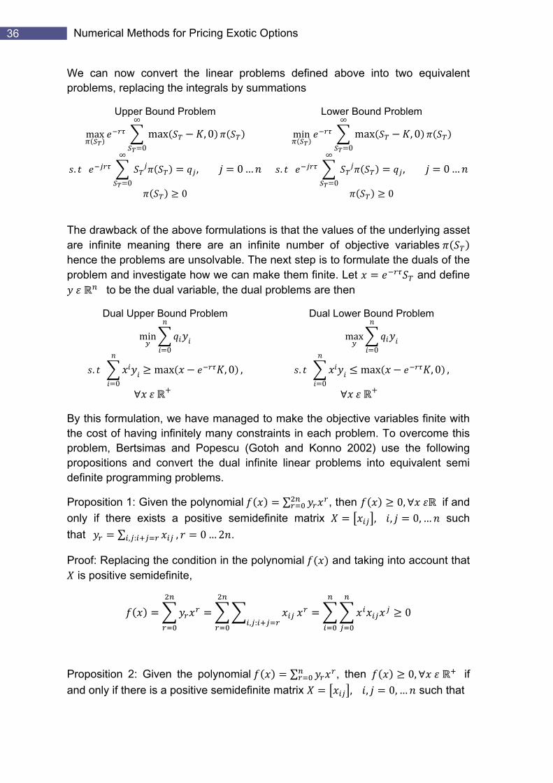
We can now convert the linear problems defined above into two equivalent problems, replacing the integrals by summations
Upper Bound Problem
max max , 0∞
0
. ∞
0, 0…
0
Lower Bound Problem
min max , 0∞
0
. ∞
0, 0…
0
The drawback of the above formulations is that the values of the underlying asset are infinite meaning there are an infinite number of objective variables hence the problems are unsolvable. The next step is to formulate the duals of the problem and investigate how we can make them finite. Let and define to be the dual variable, the dual problems are then
Dual Upper Bound Problem Dual Lower Bound Problem
min0
. 0
max , 0 ,
max0
. 0
max , 0 ,
By this formulation, we have managed to make the objective variables finite with the cost of having infinitely many constraints in each problem. To overcome this problem, Bertsimas and Popescu (Gotoh and Konno 2002) use the following propositions and convert the dual infinite linear problems into equivalent semi definite programming problems.
Proposition 1: Given the polynomial ∑ , then 0, if and only if there exists a positive semidefinite matrix , , 0, … such that ∑ , : , 0…2 .
Proof: Replacing the condition in the polynomial and taking into account that is positive semidefinite,
, :0
Proposition 2: Given the polynomial ∑ , then 0, if and only if there is a positive semidefinite matrix , , 0, … such that
37 6BBounding Option Prices by Semi definite Programming
, :, 0…
0, :
, 1…
Proof: If the condition holds and using proposition 1 we have
0 0
, , , , , ,
, ,
,
0
We use which is always greater than or equal to zero for all .
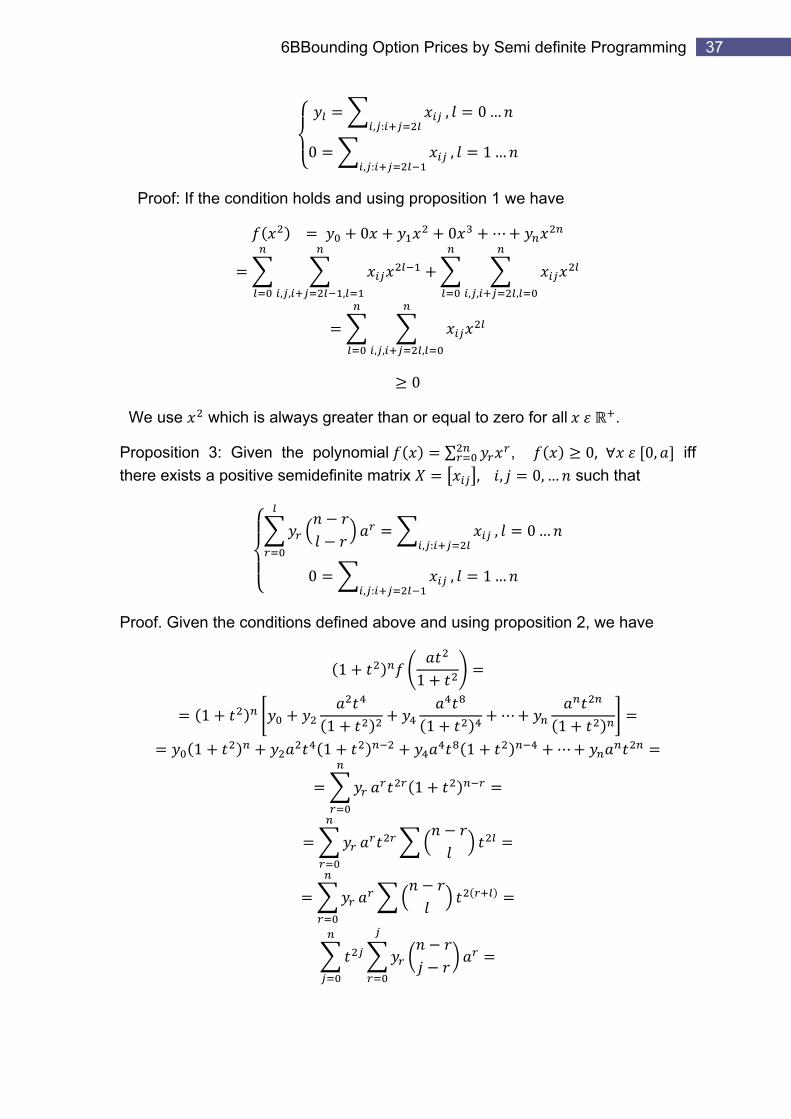
Proposition 3: Given the polynomial ∑ , 0, 0, iff there exists a positive semi e matrix , , 0, … such that definit
, :, 0…
0, :
, 1…
Proof. Given the conditions defined above and using proposition 2, we have
1 1
1 1 1 1
1 1 1
1
38 Numerical Methods for Pricing Exotic Options
,0
:
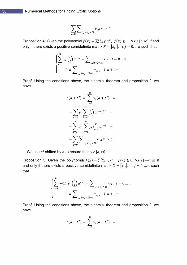
Proposition 4: Given the polynomial ∑ , 0, , ∞ if and only if there exists a positive semidefinite matrix , , 0, … such that
, :, 0…
0, :
, 1…
Proof. Using the conditions above, the binomial theorem and proposition 2, we have
, :0
We use shifted by to ensure th . at , ∞
Proposition 5: Given the polynomial ∑ , 0, ∞, if and only if there exists a positive semidefinite matrix , , 0, … such that
1, :
, 0…
0, :
, 1…
Proof. Using the conditions above, the binomial theorem and proposition 2, we have
39 6BBounding Option Prices by Semi definite Programming
1
, :0
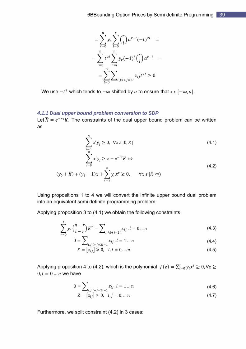
We use which tends to ∞ shifted by to ensure that ∞, .
4.1.1 Dual upper bound problem conversion to SDP Let . The constraints of the dual upper bound problem can be written as
0, 0,0
(4.1)
0
12
0, ,∞
(4.2)
Using propositions 1 to 4 we will convert the infinite upper bound dual problem into an equivalent semi definite programming problem.
Applying proposition 3 to (4.1) we obtain the following constraints
,0 …
:,
0
(4.3)
, :, 1…
0, ,
(4.4)
0,… (4.5)
Applying proposition 4 to (4.2), which is the polynomial ∑ 0,0, 0… we have
0 , :
, 1…
0, ,
(4.6)
0, … (4.7)
Furthermore, we split constraint (4.2) in 3 cases:
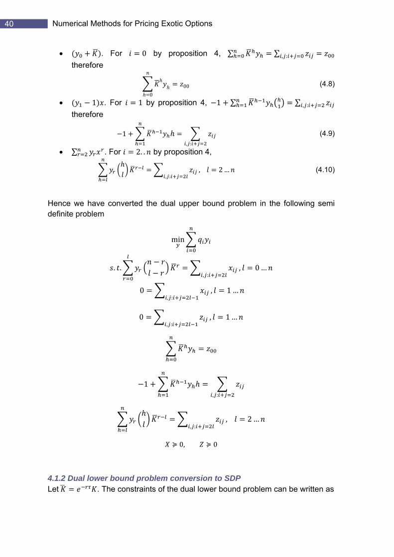
40 Numerical Methods for Pricing Exotic Options
• . For 0 by proposition 4, ∑ ∑ , : therefore
000 (4.8)
• 1 . For 1 by proposition 4, 1 ∑ ∑ , : therefore
, :
1
• ∑ 2. .
(4.9)
. For by proposition 4,
, :, 2… (4.10)
Hence we have converted the dual upper bound problem in the following semi definite problem
min
. ., :
, 0…
0, :
, 1 …
0, :
, 1…
1, :
, :, 2…
0, 0
4.1.2 Dual lower bound problem conversion to SDP Let . The constraints of the dual lower bound problem can be written as

41 6BBounding Option Prices by Semi definite Programming
0
0, 0, (4.11)
0
12
0, ,∞ (4.12)
Applying proposition 3 to (4.11) we obtain the following constraints
0… , :
,
0
(4.13)
, :, 1…
0, ,
(4.14)
0,… (4.15)
Applying proposition 4 to (4.12), which is the polynomial ∑0, 0, 0… we have
0 , :
, 1…
0, ,
(4.16)
0, … (4.17)
Further e split co int (4.12) in 3 casesmor , we nstra :
• . For 0 by proposition 4, ∑ ∑ , : therefore
000 (4.18)
• 1 . For 1 by proposition 4, 1 ∑ ∑ , : therefore
1, :
• ∑ 2
(4.19)
. For . . by proposition 4,
, :, 2… (4.20)
Hence we have converted the dual lower bound problem in the following semi definite problem
42 Numerical Methods for Pricing Exotic Options
max
. ., :
, 0…
0, :
, 1 …
0, :
, 1…
1, :
, :, 2…
0, 0
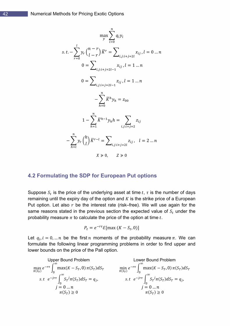
4.2 Formulating the SDP for European Put options
Suppose is the price of the underlying asset at time , is the number of days remaining until the expiry day of the option and is the strike price of a European Put option. Let also be the interest rate (risk–free). We will use again for the same reasons stated in the previous section the expected value of under the probability measure to calculate the price of the option at time .
max , 0
Let , 0, … be the first moments of the probability measure . We can formulate the following linear programming problems in order to find upper and lower bounds on the price of the Pall option.
Upper Bound Problem
max max , 0∞
0
. ∞
0,
0… 0
Lower Bound Problem
min max , 0∞
0
. ∞
0,
0…0
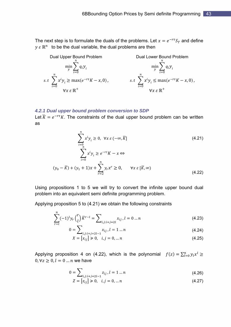
43 6BBounding Option Prices by Semi definite Programming
The next step is to formulate the duals of the problems. Let and define to be the dual variable, the dual problems are then
Dual Upper Bound Problem Dual Lower Bound Problem
min0
. 0
max , 0 ,
min0
. 0
max , 0 ,
4.2.1 Dual upper bound problem conversion to SDP Let . The constraints of the dual upper bound problem can be written as
0
0, ∞, (4.21)
0
12
0, ,∞ (4.22)
Using propositions 1 to 5 we will try to convert the infinite upper bound dual problem into an equivalent semi definite programming problem.
Applying p oposition 5 to (4.21) we obtain the following constraints r
1 0… , :
,
0
(4.23)
, :, 1…
0, ,
(4.24)
0,… (4.25)
Applying proposition 4 on (4.22), which is the polynomial ∑0, 0, 0… ave we h
0 , :
, 1…
0, ,
(4.26)
0, … (4.27)
44 Numerical Methods for Pricing Exotic Options
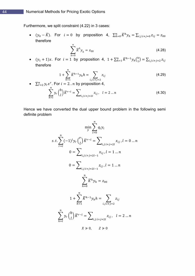
Furthermore, we split constraint (4.22) in 3 cases:
• . For 0 by proposition 4, ∑ ∑ , : therefore
000 (4.28)
• 1 . For 1 by proposition 4, 1 ∑ ∑ , : therefore
1, :
• ∑ 2. .
(4.29)
. For by proposition 4,
, :, 2… (4.30)
Hence we have converted the dual upper bound problem in the following semi definite problem
min
. . 1, :
, 0…
0, :
, 1 …
0, :
, 1…
1, :
, :, 2…
0, 0
45 6BBounding Option Prices by Semi definite Programming
4.2.2 Dual lower bound problem conversion to SDP Let . The constraints of the dual lower bound problem can be written as
0, ∞,0
(4.31)
0
12
0, ,∞ (4.32)
Applying pr position to (4.31) we obtain the following constraints o 5
1:
0… ,
,
0
(4.33)
, :, 1 …
0, ,
(4.34)
0,… (4.35)
Applying proposition 4 on (4.32), which is the polynomial ∑0, 0, 0… ave we h
0 , :
, 1…
0, ,
(4.36)
0, … (4.37)
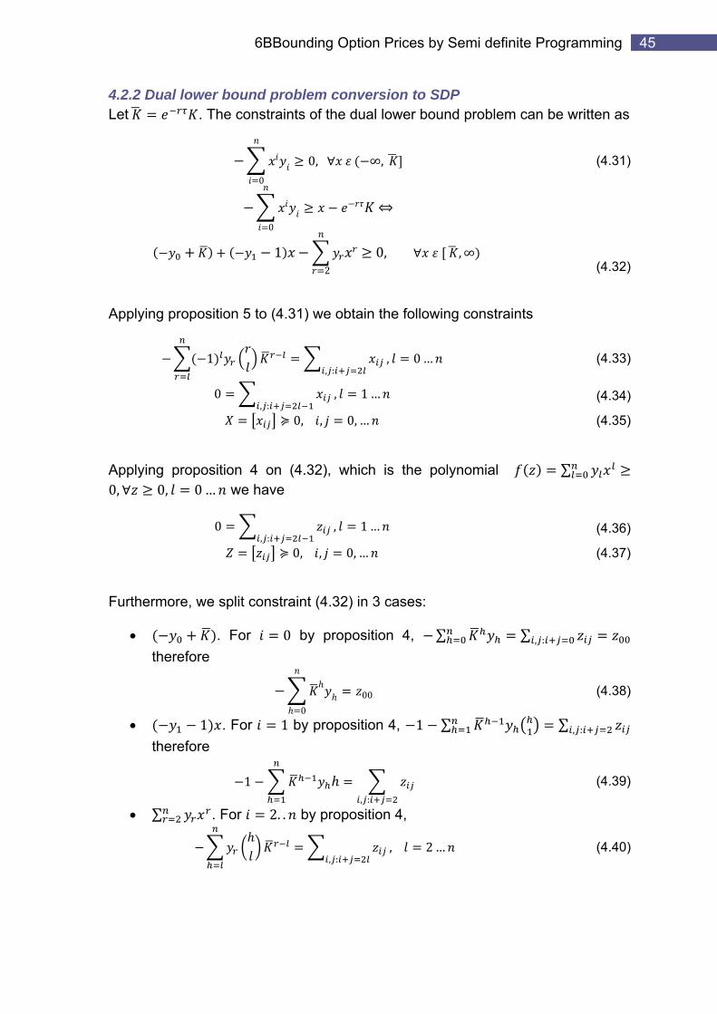
Further e split co int (4.32) in 3 casesmor , we nstra :
• . For 0 by proposition 4, ∑ ∑ , : therefore
000
• 1 . For 1 by proposition 4, 1 ∑ ∑ , : therefore
(4.38)
, :
1
• ∑ . .
(4.39)
. For 2 by proposition 4,
, :, 2… (4.40)
46 Numerical Methods for Pricing Exotic Options
Hence we have converted the dual lower bound problem in the following semi definite problem
max
. . 1, :
, 0…
0, :
, 1 …
0, :
, 1…
1, :
, :, 2…
0, 0
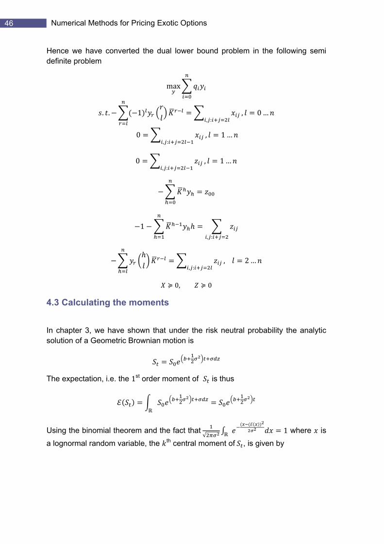
4.3 Calculating the moments
In chapter 3, we have shown that under the risk neutral probability the analytic solution of a Geometric Brownian motion is
The expectation, i.e. the 1st order moment of is thus
Using the binomial theorem and the fact that √
1 where is
a lognormal random variable, the th central moment of , is given by
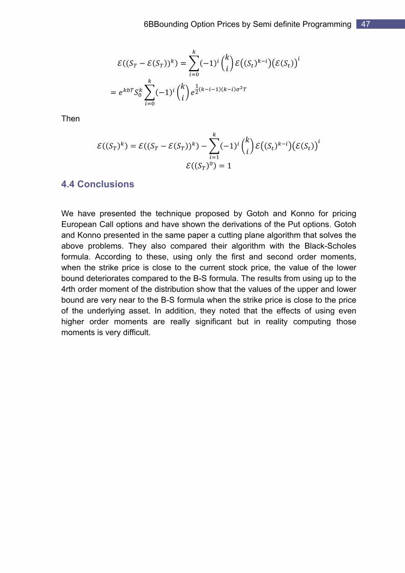
47 6BBounding Option Prices by Semi definite Programming
1
1
Then
1
1
4.4 Conclusions
We have presented the technique proposed by Gotoh and Konno for pricing European Call options and have shown the derivations of the Put options. Gotoh and Konno presented in the same paper a cutting plane algorithm that solves the above problems. They also compared their algorithm with the Black-Scholes formula. According to these, using only the first and second order moments, when the strike price is close to the current stock price, the value of the lower bound deteriorates compared to the B-S formula. The results from using up to the 4rth order moment of the distribution show that the values of the upper and lower bound are very near to the B-S formula when the strike price is close to the price of the underlying asset. In addition, they noted that the effects of using even higher order moments are really significant but in reality computing those moments is very difficult.
48 Numerical Methods for Pricing Exotic Options
Chapter 5
Pricing a Class of Exotic Options via Moments and SDP relaxations
In this chapter, we investigate the methodology proposed by Lasserre, Prieto-Rumeau and Zervos for pricing Asian and Barrier options. They apply the problem of moments for polynomial optimization deriving semi definite programming problems which when solved, give tight upper and lower bounds for the prices of the derivatives. They assume that the underlying asset follows a number of different processes. In the following sections, we will present the general method and then show how it can be adapted for each class of options.
5.1 Formulating the problem
Consider an -dimentional diffusion process defined on the probability space , , , is a σ-algebra on , given by the following stochastic differential equ oati n
, , : ,
We require that this SDE has a strong solution, for example it can be the Geometric Brownian motion, where we have shown the solution in previous chapters. Is an -dimentional Weiner process. The infinitesimal generator of process is given by
z12 z , ε D A
Domain D A contains all the functions whose second derivatives exist for all z. Process can be any process whose infinitesimal generator maps polynomials over polynomials, hence and must be polynomials. In fact this is the first restriction of this method. If we think that process is the price of the underlying asset, then we can use any model which satisfies this condition for our options.
If , are multi-indices, we can define to be the monomial
(5.1)
49 7BPricing a Class of Exotic Options via Moments and SDP relaxations
Then we can see that is a polynomial with real coefficients, i.e.
(5.2)
Furthermore, we require that the sum of all same order moments over all dimensions of is finite, i.e.
sup ,
∞ , 0,
Doob’s optional sampling theorem (Karatzas and Shreve 1991). Let a process be a martingale , . Let be a stopping time with respect to . If process
is finite, i.e. there is a last element in the sequence, then .
Define the martingale process
M , : ,
If is a stopping time with respect to M , then according to Doob’s optional sampling theorem
M M 0
0
0
0
(5.3)
We then need to define two measures for the diffusion .
The exit location measur o on of is given by e, i.e. the pr bability distributi
,
The expected occupation measur up to the stopping time τ is given by e
,
50 Numerical Methods for Pricing Exotic Options
is an indicator function of th re fo m
1, 0,
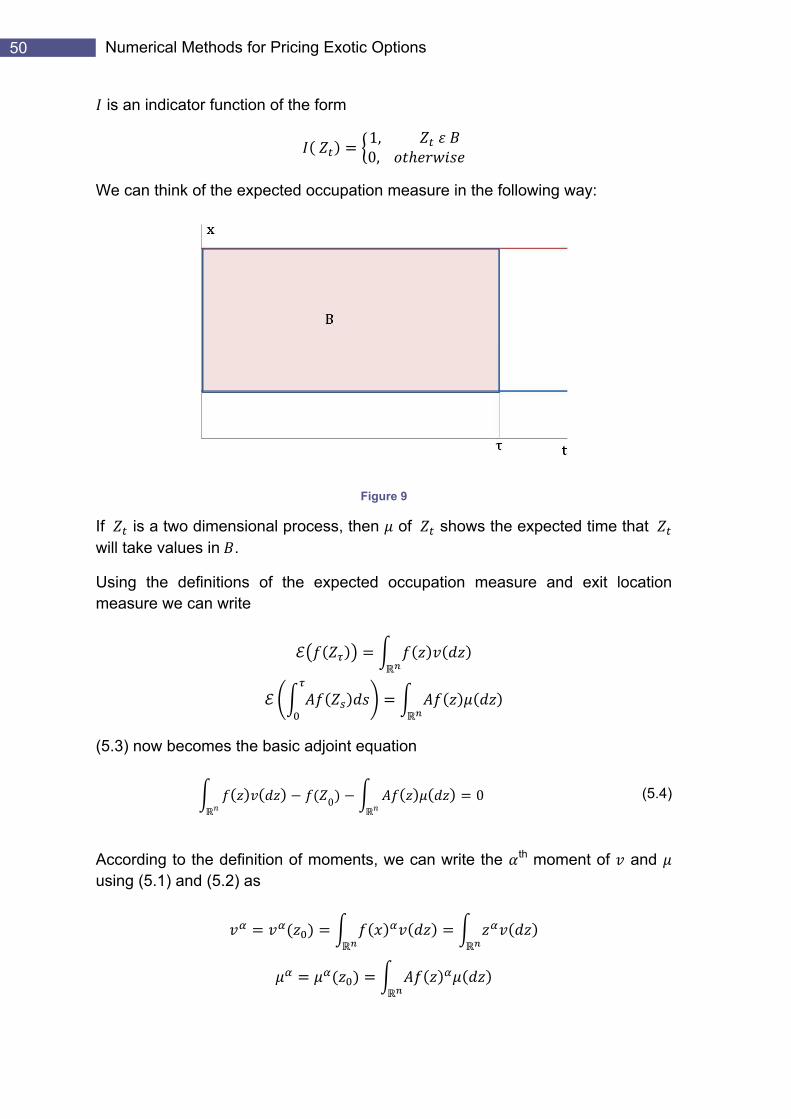
We can think of the expected occupation measure in the following way:
Figure 9
If is a two dimensional process, then of shows the expected time that will take values in .
Using the definitions of the expected occupation measure and exit location measure we can write
(5.3) now becomes the basic adjoint equation
0 0 (5.4)
According to the definition of moments, we can write the th moment of and using (5.1) and (5.2) as
51 7BPricing a Class of Exotic Options via Moments and SDP relaxations
We assume that these moments exist and are finite. The basic adjoint equation (5.4) now becomes an infinite system of linear equations
0 (5.5)
In the problem of moments, we are interested in finding the maximum and/or the minimum of a function defined as
is a measure defined on a σ-algebra on and : is a polynomial with real coefficients.
In finance, we have shown that the price of an option whose underlying asset is modelled by is given by the functional
,
where is the exit location measure and and are real valued polynomials defined as
, 1…
If we partition in measures supported on for all 1… such that
and define to be the th moment of , then we can rewrite as
Hence, in the context of the problem of moments, we want to extremize . In addition, we have some information about the moments as we saw in the
52 Numerical Methods for Pricing Exotic Options
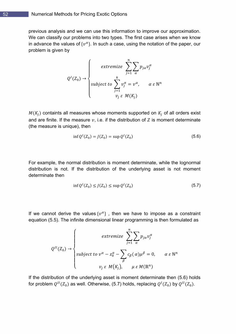
previous analysis and we can use this information to improve our approximation. We can classify our problems into two types. The first case arises when we know in advance the values of . In such a case, using the notation of the paper, our problem is given by
,
containts all measures whose moments supported on of all orders exist and are finite. If the measure , i.e. if the distribution of is moment determinate (the measure is uniqu h ne), t e
inf sup (5.6)
For example, the normal distribution is moment determinate, while the lognormal distribution is not. If the distribution of the underlying asset is not moment determinate then
inf sup (5.7)
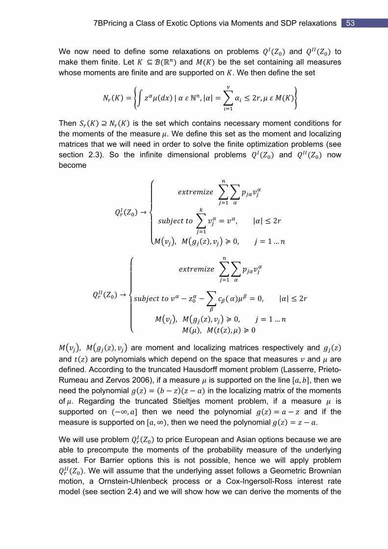
If we cannot derive the values , then we have to impose as a constraint equation (5.5). The in nite dimensional linear programming is then formulated as fi
0,
,
If the distribution of the underlying asset is moment determinate then (5.6) holds for problem as well. Otherwise, (5.7) holds, replacing by .
53 7BPricing a Class of Exotic Options via Moments and SDP relaxations
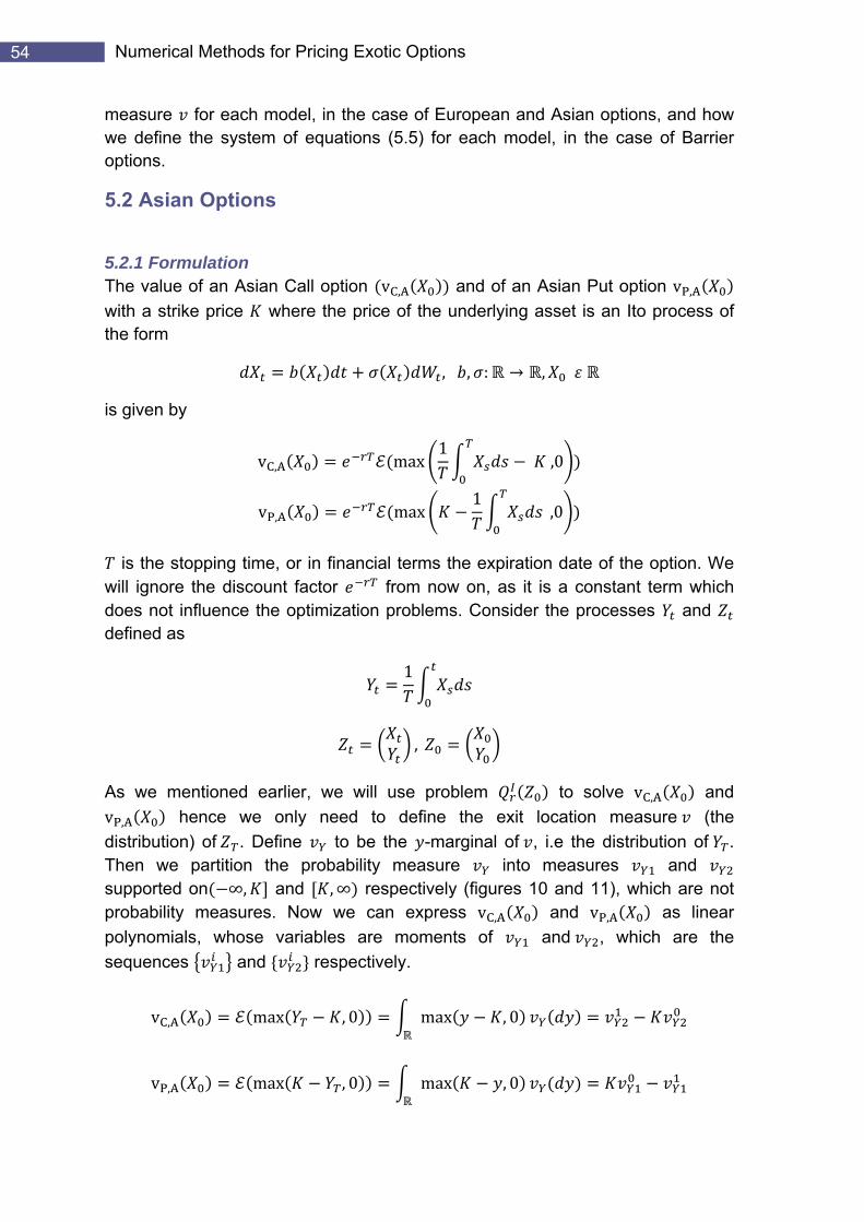
We now need to define some relaxations on problems and to make them finite. Let and be the set containing all measures whose moments are finite and are supported on . We then define the set
| , | | 2 ,
Then is the set which contains necessary moment conditions for the moments of the measure . We define this set as the moment and localizing matrices that we will need in order to solve the finite optimization problems (see section 2.3). So the infinite dimensional problems and now become
, | | 2
, , 0, 1…
0, | | 2
, , 0, 1…, , 0
, , are moment and localizing matrices respectively and and are polynomials which depend on the space that measures and are defined. According to the truncated Hausdorff moment problem (Lasserre, Prieto-Rumeau and Zervos 2006), if a measure is supported on the line , , then we need the polynomial in the localizing matrix of the moments of . Regarding the truncated Stieltjes moment problem, if a measure is supported on ∞, then we need the polynomial and if the measure is supported ∞ , then we need the polynomial . on ,
We will use problem to price European and Asian options because we are able to precompute the moments of the probability measure of the underlying asset. For Barrier options this is not possible, hence we will apply problem
. We will assume that the underlying asset follows a Geometric Brownian motion, a Ornstein-Uhlenbeck process or a Cox-Ingersoll-Ross interest rate model (see section 2.4) and we will show how we can derive the moments of the
54 Numerical Methods for Pricing Exotic Options
measure for each model, in the case of European and Asian options, and how we define the system of equations (5.5) for each model, in the case of Barrier options.
5.2 Asian Options
5.2.1 Formulation The value of an Asian Call option vC,A and of an Asian Put option vP,A with a strike price where the price of the underlying asset is an Ito process of the form
, , : ,
is given by
vC,A max1
,0
vP,A max1
,0
is the stopping time, or in financial terms the expiration date of the option. We will ignore the discount factor from now on, as it is a constant term which does not influence the optimization problems. Consider the processes and defined as
1
,
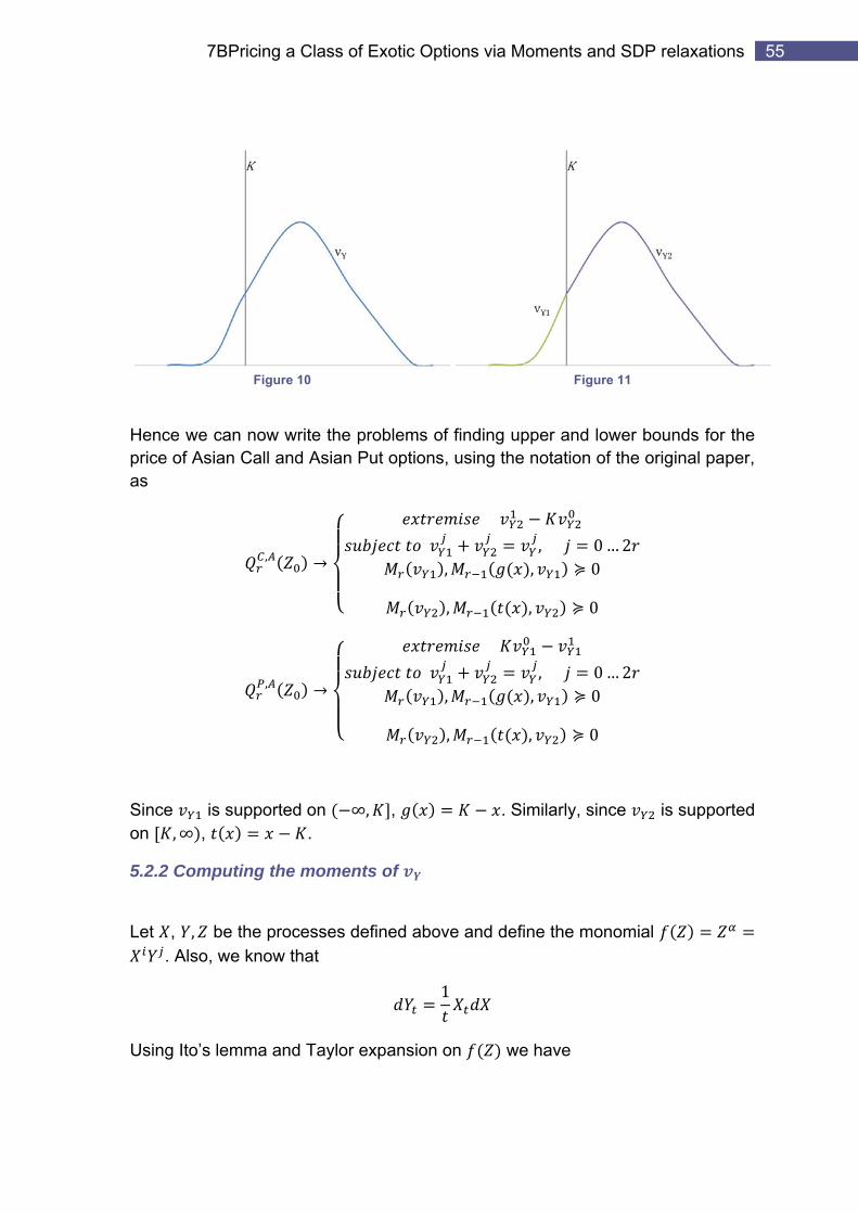
As we mentioned earlier, we will use problem to solve vC,A and vP,A hence we only need to define the exit location measure (the distribution) of . Define to be the -marginal of , i.e the distribution of . Then we partition the probability measure into measures and supported on ∞, and , ∞ respectively (figures 10 and 11), which are not probability measures. Now we can express vC,A and vP,A as linear polynomials, whose variables are moments of and , which are the sequences and respectively.
vC,A max , 0 max , 0
vP,A max , 0 max , 0
55 7BPricing a Class of Exotic Options via Moments and SDP relaxations
Figure 10 Figure 11
Hence we can now write the problems of finding upper and lower bounds for the price of Asian Call and Asian Put options, using the notation of the original paper, as
,
, 0…2
, , 0
0
, ,
,
, 0…2
, , 0
, , 0
Since is supported on ∞, , . Similarly, since is supported on , ∞ , .
5.2.2 Computing the moments of
Let , , be the processes defined above and define the monomial . Also, we know that
1
Using Ito’s lemma and Taylor expansion on we have
56 Numerical Methods for Pricing Exotic Options
,
, ,12 , 2 ,
,
If the price of the underlying asset is a Geometric Brownian motion then is given by the stochastic differe iant l equation
Then
,1
12 1
21
11
is a Weiner process hence √ , ~ 0,1 and remembering the fact in Ito’s lemma, we keep only the terms with order ∆t or smaller, then
,1
12 1
If we define the moments of to be , and taking into account that the moments of are , , then we can find those moments by solving the following system of ordinary differential equations
, , 1 , 12 1 ,
0 2 , 0 0, 0
, 0 1 , 0
If the price of the underlying asset is the Ornstein-Uhlenbeck process then is given by the stochastic differential equation
Then
,1
12 1
57 7BPricing a Class of Exotic Options via Moments and SDP relaxations
The sy t m o q n thus s e of rdinary differential e uatio s is
, , , 1 , 12 1 ,
0 2 , 0 0, 0
, 0 1 , 0
If the price of the underlying asset is the Cox-Ingersoll-Ross interest rate model then is given by e e tion the stochastic diff r ntial equa
Then
, √1
12 1
The s s m fy te o ordinary differential equations is thus
, , , 1 , 12 1 ,
0 2 , 0 0, 0
, 0 1 , 0
5.3 European Options
5.3.1 Formulation The analysis for European Call options is similar to Asian Options. The value of a European Call option vC,E and of a European Put option vP,E with a strike price whe th e t t cess of the form re e pric of the underlying asse is an I o pro
, , : ,
is given by
vC,E max ,0 vP,E max ,0
is the stopping time. We will again ignore the discount factor .
58 Numerical Methods for Pricing Exotic Options
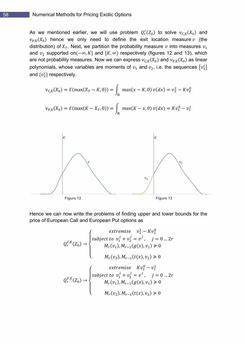
As we mentioned earlier, we will use problem to solve vC,E and vP,E hence we only need to define the exit location measure (the distribution) of . Next, we partition the probability measure into measures and supported on ∞, and , ∞ respectively (figures 12 and 13), which are not probability measures. Now we can express vC,E and vP,E as linear polynomials, whose variables are moments of and , i.e. the sequences and respectively.
vC,E max , 0 max , 0
vP,E max , 0 max , 0
Figure 12 Figure 13
Hence we can now write the problems of finding upper and lower bounds for the price of European Call and European Put options as
,
, 0…2
, , 0
0
, ,
,
, 0…2
, , 0
, , 0
59 7BPricing a Class of Exotic Options via Moments and SDP relaxations
Since is supported on ∞, , . Similarly, since is supported on , ∞ , .
5.3.2 Computing the moments of
Let be the processe defined above and define the monomial .
Using Ito’s lemma an we have d Taylor expansion on
12
If the price of the underlying asset is a Geometric Brownian motion then is given by the stochastic differe iant l equation
and 12 1
is a Weiner process hence √ , ~ 0,1 and remembering the fact in Ito’s lemma, we k n h e w ave eep o ly the terms wit ord r ∆t or smaller, e h
12 1
If we define the moments of to be then we can find those moments by solving the following system of ordinary differential equations
12 1
0 2 0
If the price of the underlying asset is the Ornstein-Uhlenbeck process then is given by the stochastic differential equation
Then 12 1
The system of dinary differentiaor l equations is thus
, 12 1
0 2
60 Numerical Methods for Pricing Exotic Options
0
If the price of the underlying asset is the Cox-Ingersoll-Ross interest rate model then is given by e e tion the stochastic diff r ntial equa
In this case,
12 1
The system of dinary differentiaor l equations is thus
, 12 1
0 2 0
5.4 Barrier Options
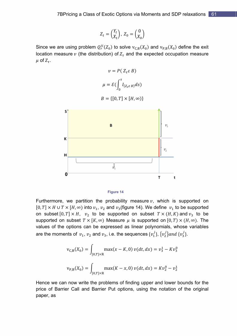
5.4.1 Formulation For down-and-out Barrier options, we will need to formulate the problem because, as we will see, we will not be able to calculate the moments of the exit location measure. Recall that the value of a Barrier Call option vC,B and of a Barrier Put option vP,B with a strike price and barrier where the price of the underlying as i oset s an It process of the form
, , : ,
is given by
vC,B max ,0 vP,B max ,0
is the stopping time defined as
min 0|
The stopping time will either be the expiration date of the option or the time that the price of the underlying falls below the barrier. We will again ignore the discount factor . Consider the o and defined as pr cesses
, 0
7BPPricing a CClass of Exotic Optionns via Momments and SDP relax
Sinloca
of
Fur0,
on supvaluare
Henpricpap
ce we are ation measf .
rthermore,
subset 0,pported onues of the the mome
nce we cace of Barriper, as
using prosure (the
we partit, ∞ in
, , subset options c
ents of ,
vC,B
vP,B
n now writier Call an
blem e distributio
tion the pnto , a
to be, ∞ M
can be exp and ,
m,
m,
te the probnd Barrier
,
to solveon) of a
0,
Figure 14
probability and (figusupported
Measure pressed as, i.e. the se
max , 0
max ,
blems of finPut option
0
e vC,Bnd the exp
, ∞
measure ure 14). We on subs is suppo
s linear poequences
0 ,
0 ,
nding uppens, using
and vP,Bpected occ
, which e define
set ,orted on 0,olynomials,
,
er and lowthe notatio
define cupation m
xations 61
the exit measure
is suppor to be sup, and , , ∞ whose va .
rted on pported to be ∞ . The ariables
wer boundson of the
s for the original
62 Numerical Methods for Pricing Exotic Options
,
, ,
,
, , 0 , 0 2
, , 0
, , 0, , 0
, , 0
, ,
,
, ,
,
, , 0 , 0 2
, , 0
, , 0, , 0
, , , , 0
Since is supported on 0, , 0 . Similarly, since is supported on , , , . The marginal
of is supported on 0, hence and the marginal of is supported on , ∞ hence .
Finally, we need to define the system of equations
, ,
,
, , 0 , 0 2
Recall that the above equation is derived from (5.4)
0
, :
Now we know that for any model we have
, ,
63 7BPricing a Class of Exotic Options via Moments and SDP relaxations
The coefficients
,
, ,
are model specific, since they depend on how and are defined
5.4.2 Defining the moments If the price of the underlying asset is a Geometric Brownian motion then is given by the stochastic differe iant l equation
Hence we can write
,12 1
,
, , , 12 1 , ,
If the price of the underlying asset is the Ornstein-Uhlenbeck process then is given by the stochastic differential equation
Then
,12 1
,
, , , 12 1 , , ,
If the price of the underlying asset is the Cox-Ingersoll-Ross interest rate model then is given by e e tion the stochastic diff r ntial equa
Then
,12 √ 1
64 Numerical Methods for Pricing Exotic Options
,
, , , 12 1 , , ,
65 Numerical Results
Chapter 6
Numerical Results
In this chapter we will demonstrate the results we obtained by implementing some of the methods we investigated. We use Matlab to write our programs. First, we compare the method proposed by Bertsimas and Popescu and the method proposed by Lasserre, Prieto-Rumeau and Zervos for pricing European Options against the Black-Scholes PDE. Then we will analyze the results we obtained by implementing the methods for pricing Asian options.
6.1 Software and Hardware
Matlab, created by “The MathWorks”, is a high performance language for writing algorithms and analysing data using graphics. Its name stands for Matrix Laboratory because the basic element of Matlab is an array. This enables the users to write technical problems, involving computations of matrices and vectors, very fast. It provides a huge library of mathematical functions and operations, such as integration. The key advantage of Matlab compared to high-level languages (ex. Java, C# ) is that it is capable of performing very fast complex computations. As the scope of this project was not to create a complete application rather to experiment with the algorithms, we decided to use Matlab. A wide variety of open source SDP solvers exist that would help us with the optimization problems of the algorithms. We used Sedumi which is an optimization package specifically designed to be compatible with Matlab. As an interface for Sedumi, we used Yalmip1, which is open source as well. Yalmip enabled us to easily create the optimization problems, focusing on high level design.
We ran our experiments on a 2.10GHz Intel® Core™ 2 Duo T8100 with 2GB RAM running 32-bit Windows Vista™ Home Premium.
6.2 Pricing a Class of Exotic Options via Moments and SDP relaxations
6.2.1 European Call options The following graphs plot the number of relaxations against the values of European Call options using Lasserre’s method. We used the same dataset as Lasserre in order to verify our results. We were able to obtain tight upper and 1 http://control.ee.ethz.ch/~joloef/yalmip.php
66 Numerical Methods for Pricing Exotic Options
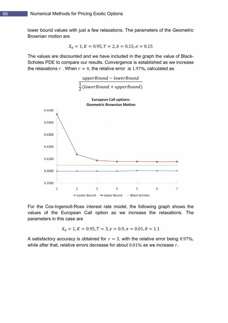
lower bound values with just a few relaxations. The parameters of the Geometric Brownian motion are
1, 0.95, 2, 0.15, 0.15
The values are discounted and we have included in the graph the value of Black-Scholes PDE to compare our results. Convergence is established as we increase the relaxations . When %, calculated as 4, the relative error is 1.97
12
For the Cox-Ingersoll-Ross interest rate model, the following graph shows the values of the European Call option as we increase the relaxations. The parameters in thi c es ase ar
1, 0.95, 3 .9, 0.01, 1.1 , 0
A satisfactory accuracy is obtained for 3, with the relative error being 0.97%, while after that, relative errors decrease for about 0.01% as we increase .

67 Numerical Results
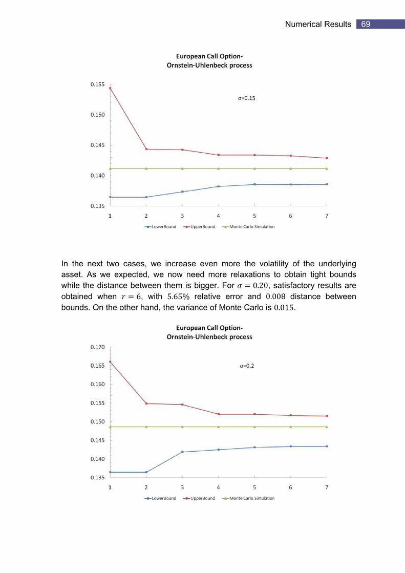
For the Ornstein-Uhlenbeck process, we have compared our results against Monte Carlo simulation, for a range of volatilites. As we see, Monte Carlo lies between the upper and lower bounds we obtained. Furthermore, as we increase the volatility of the underlying asset, the distance between the bounds increases. The parameters of this r model a e
1, 0.95, 2, 1, 1.1
The level of volatility is shown on the graphs.
68 Numerical Methods for Pricing Exotic Options
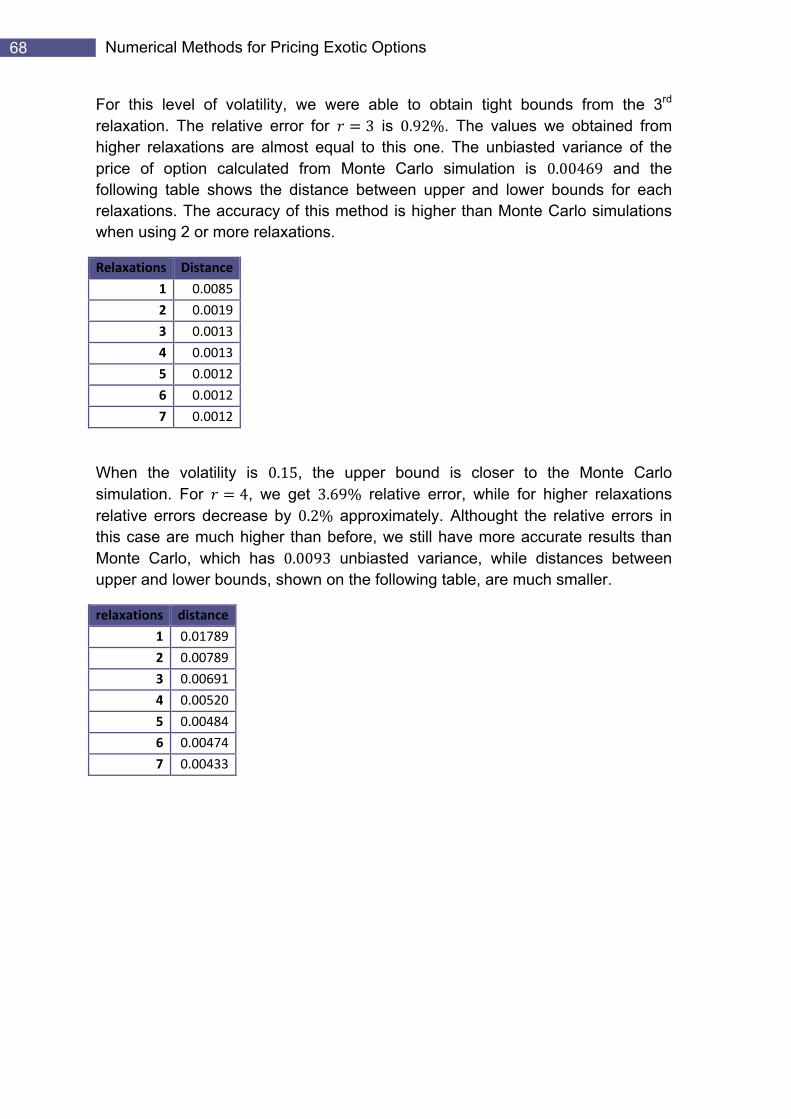
For this level of volatility, we were able to obtain tight bounds from the 3rd relaxation. The relative error for 3 is 0.92%. The values we obtained from higher relaxations are almost equal to this one. The unbiasted variance of the price of option calculated from Monte Carlo simulation is 0.00469 and the following table shows the distance between upper and lower bounds for each relaxations. The accuracy of this method is higher than Monte Carlo simulations when using 2 or more relaxations.
Relaxations Distance
1 0.0085
2 0.0019
3 0.0013
4 0.0013
5 0.0012
6 0.0012
7 0.0012
When the volatility is 0.15, the upper bound is closer to the Monte Carlo simulation. For 4, we get 3.69% relative error, while for higher relaxations relative errors decrease by 0.2% approximately. Althought the relative errors in this case are much higher than before, we still have more accurate results than Monte Carlo, which has 0.0093 unbiasted variance, while distances between upper and lower bounds, shown on the following table, are much smaller.
relaxations distance
1 0.01789
2 0.00789
3 0.00691
4 0.00520
5 0.00484
6 0.00474
7 0.00433
69 Numerical Results
In the next two cases, we increase even more the volatility of the underlying asset. As we expected, we now need more relaxations to obtain tight bounds while the distance between them is bigger. For 0.20, satisfactory results are obtained when 6, with 5.65% relative error and 0.008 distance between bounds. On the other hand, the variance of Monte Carlo is 0.015.
70 Numerical Methods for Pricing Exotic Options
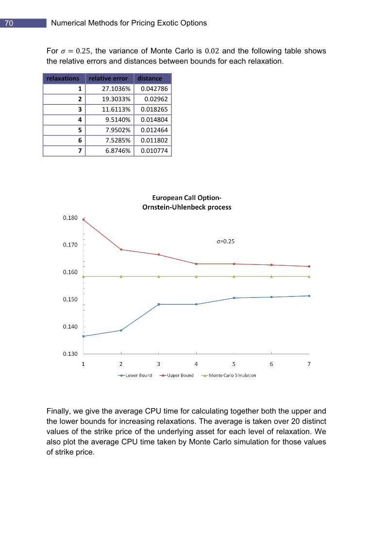
For 0.25, the variance of Monte Carlo is 0.02 and the following table shows the relative errors and distances between bounds for each relaxation.
relaxations relative error distance
1 27.1036% 0.042786
2 19.3033% 0.02962
3 11.6113% 0.018265
4 9.5140% 0.014804
5 7.9502% 0.012464
6 7.5285% 0.011802
7 6.8746% 0.010774
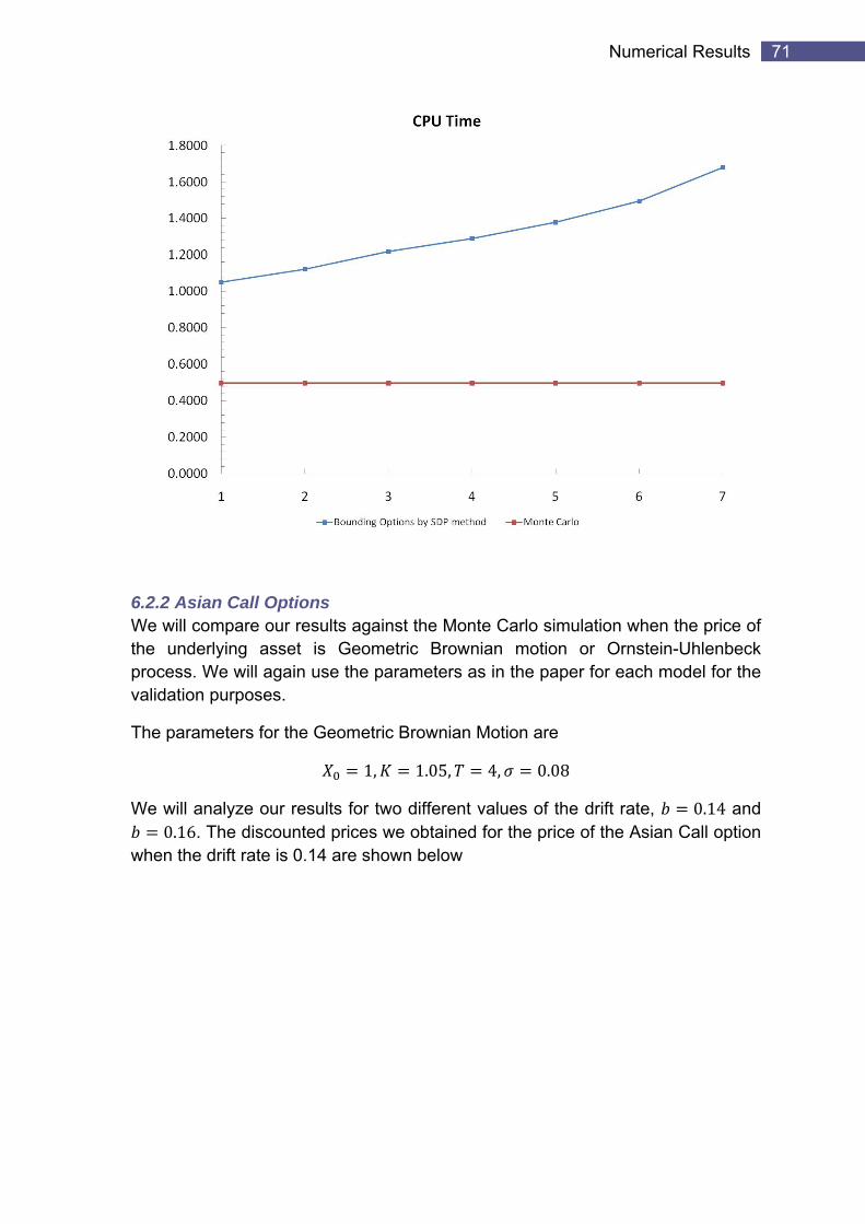
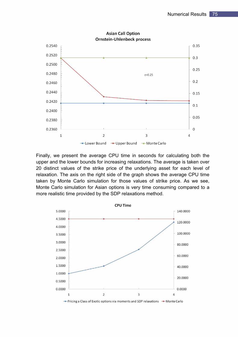
Finally, we give the average CPU time for calculating together both the upper and the lower bounds for increasing relaxations. The average is taken over 20 distinct values of the strike price of the underlying asset for each level of relaxation. We also plot the average CPU time taken by Monte Carlo simulation for those values of strike price.
71 Numerical Results
6.2.2 Asian Call Options We will compare our results against the Monte Carlo simulation when the price of the underlying asset is Geometric Brownian motion or Ornstein-Uhlenbeck process. We will again use the parameters as in the paper for each model for the validation purposes.
The parameters for the G oe metric Brownian Motion are
1, 1.05, 4, 0.08
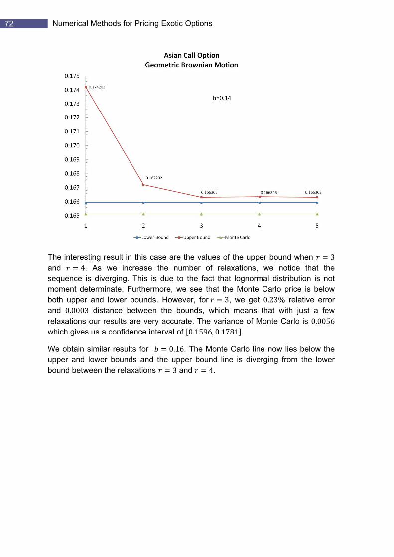
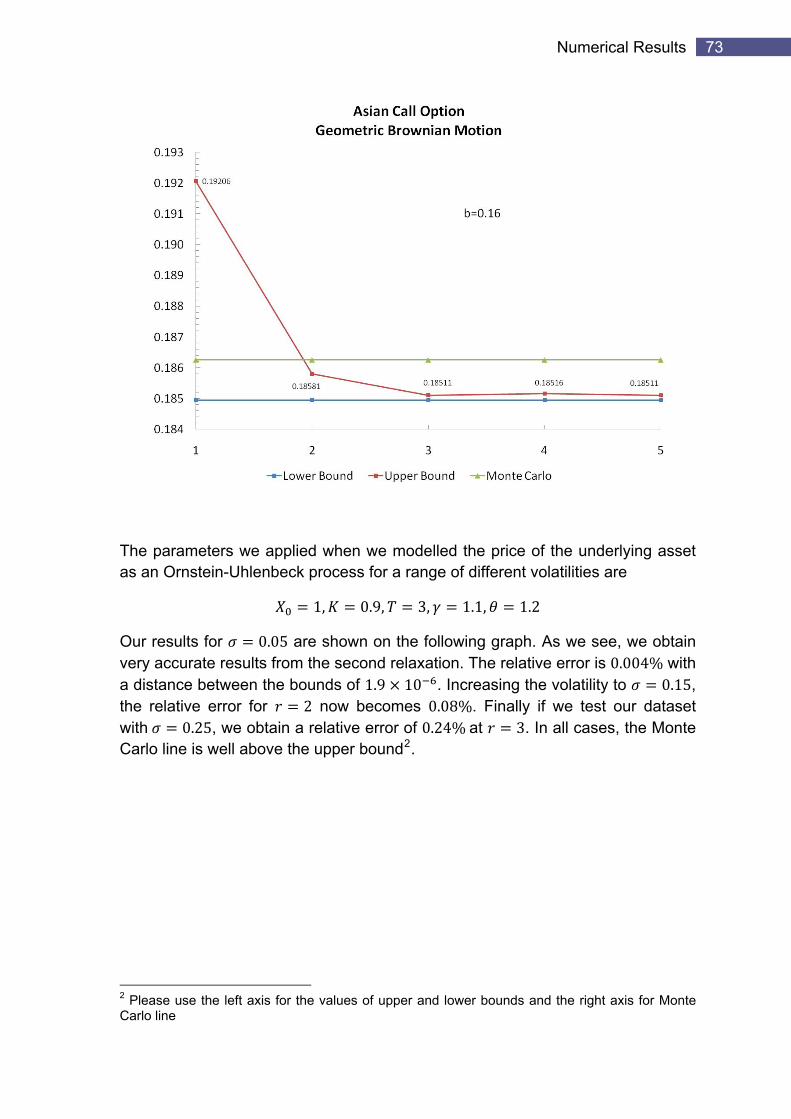
We will analyze our results for two different values of the drift rate, 0.14 and 0.16. The discounted prices we obtained for the price of the Asian Call option
when the drift rate is 0.14 are shown below
72 Numerical Methods for Pricing Exotic Options
The interesting result in this case are the values of the upper bound when 3 and 4. As we increase the number of relaxations, we notice that the sequence is diverging. This is due to the fact that lognormal distribution is not moment determinate. Furthermore, we see that the Monte Carlo price is below both upper and lower bounds. However, for 3, we get 0.23% relative error and 0.0003 distance between the bounds, which means that with just a few relaxations our results are very accurate. The variance of Monte Carlo is 0.0056 which gives us a confidence in 0.1596, 0.1781 . terval of
We obtain similar results for 0.16. The Monte Carlo line now lies below the upper and lower bounds and the upper bound line is diverging from the lower bound between the relaxations 3 and 4.
73 Numerical Results
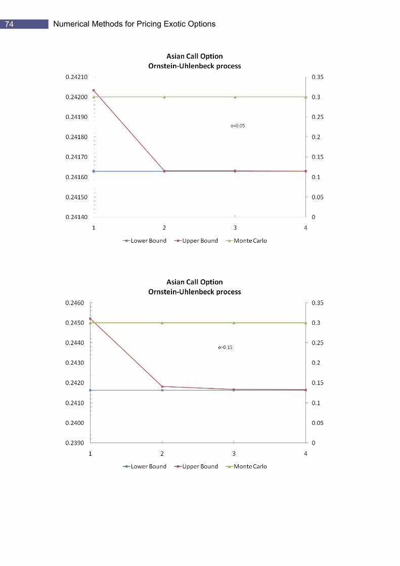
The parameters we applied when we modelled the price of the underlying asset as an Ornstein-Uhlenb c latilities are e k process for a range of different vo
1, 0.9, 3, 1.1, 1.2
Our results for 0.05 are shown on the following graph. As we see, we obtain very accurate results from the second relaxation. The relative error is 0.004% with a distance between the bounds of 1.9 10 . Increasing the volatility to 0.15, the relative error for 2 now becomes 0.08%. Finally if we test our dataset with 0.25, we obtain a relative error of 0.24% at 3. In all cases, the Monte Carlo line is well above the upper bound2.
2 Please use the left axis for the values of upper and lower bounds and the right axis for Monte Carlo line
74 Numerical Methods for Pricing Exotic Options
75 Numerical Results
Finally, we present the average CPU time in seconds for calculating both the upper and the lower bounds for increasing relaxations. The average is taken over 20 distinct values of the strike price of the underlying asset for each level of relaxation. The axis on the right side of the graph shows the average CPU time taken by Monte Carlo simulation for those values of strike price. As we see, Monte Carlo simulation for Asian options is very time consuming compared to a more realistic time provided by the SDP relaxations method.
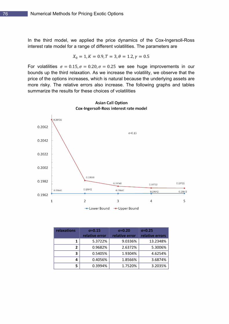
76 Numerical Methods for Pricing Exotic Options
In the third model, we applied the price dynamics of the Cox-Ingersoll-Ross interest rate model for r rameters are a ange of different volatilities. The pa
, 1.2, 0.5 1, 0.9, 3
For volatilities 0.15, 0.20, 0.25 we see huge improvements in our bounds up the third relaxation. As we increase the volatility, we observe that the price of the options increases, which is natural because the underlying assets are more risky. The relative errors also increase. The following graphs and tables summarize the results for these choices of volatilities
relaxations σ=0.15 relative error
σ=0.20 relative error
σ=0.25 relative errors
1 5.3722% 9.0336% 13.2348%
2 0.9682% 2.6372% 5.3006%
3 0.5405% 1.9304% 4.6254%
4 0.4056% 1.8566% 3.6874%
5 0.3994% 1.7520% 3.2035%
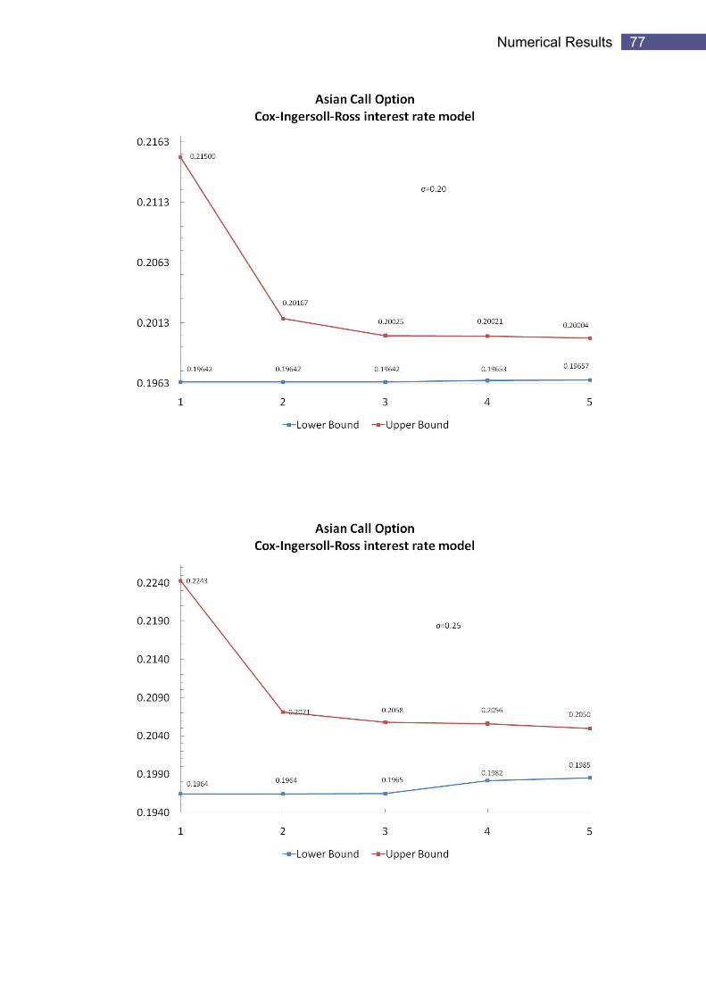
77 Numerical Results
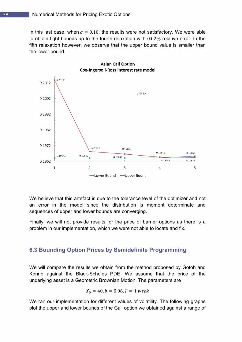
78 Numerical Methods for Pricing Exotic Options
In this last case, when 0.10, the results were not satisfactory. We were able to obtain tight bounds up to the fourth relaxation with 0.02% relative error. In the fifth relaxation however, we observe that the upper bound value is smaller than the lower bound.
We believe that this artefact is due to the tolerance level of the optimizer and not an error in the model since the distribution is moment determinate and sequences of upper and lower bounds are converging.
Finally, we will not provide results for the price of barrier options as there is a problem in our implementation, which we were not able to locate and fix.
6.3 Bounding Option Prices by Semidefinite Programming
We will compare the results we obtain from the method proposed by Gotoh and Konno against the Black-Scholes PDE. We assume that the price of the underlying asset is a Geom t o i t n arameters are e ric Br wn an Mo io . The p
40, 0.06, 1
We ran our implementation for different values of volatility. The following graphs plot the upper and lower bounds of the Call option we obtained against a range of
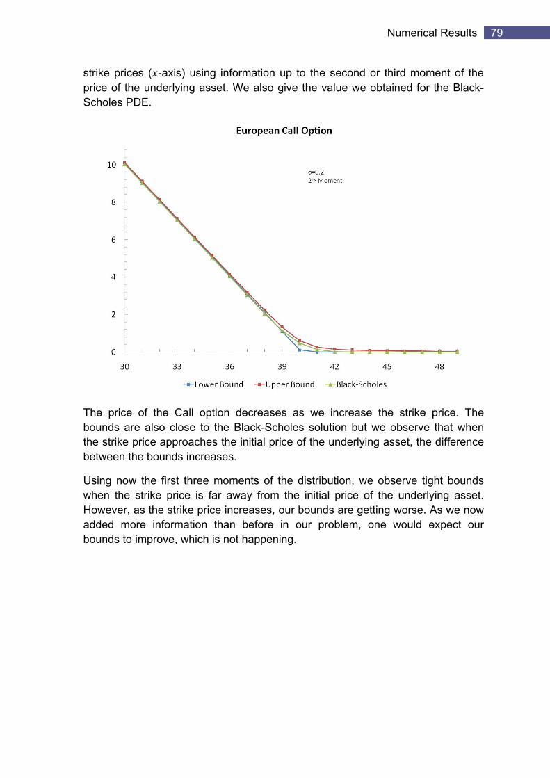
79 Numerical Results
strike prices ( -axis) using information up to the second or third moment of the price of the underlying asset. We also give the value we obtained for the Black-Scholes PDE.
The price of the Call option decreases as we increase the strike price. The bounds are also close to the Black-Scholes solution but we observe that when the strike price approaches the initial price of the underlying asset, the difference between the bounds increases.
Using now the first three moments of the distribution, we observe tight bounds when the strike price is far away from the initial price of the underlying asset. However, as the strike price increases, our bounds are getting worse. As we now added more information than before in our problem, one would expect our bounds to improve, which is not happening.
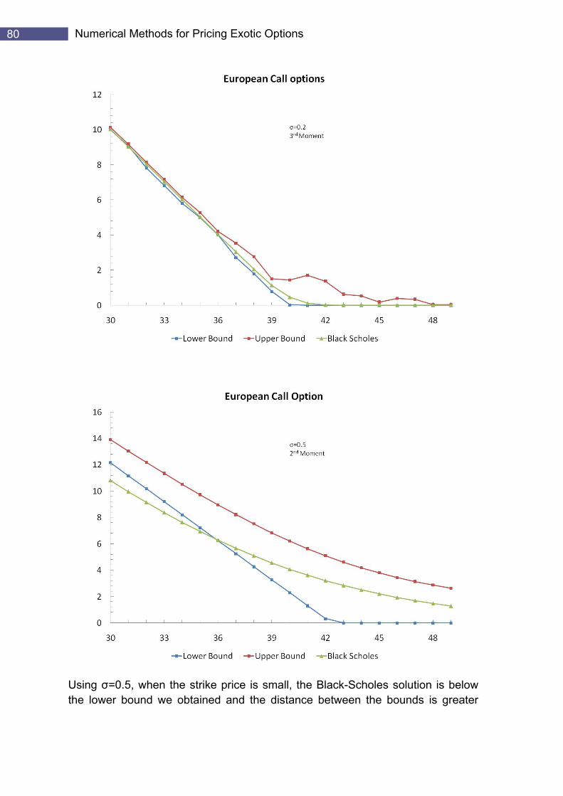
80 Numerical Methods for Pricing Exotic Options
Using σ=0.5, when the strike price is small, the Black-Scholes solution is below the lower bound we obtained and the distance between the bounds is greater
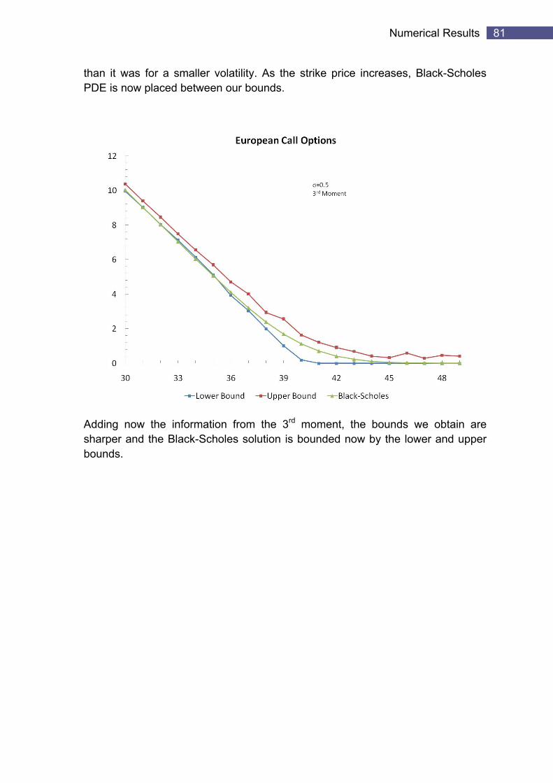
81 Numerical Results
than it was for a smaller volatility. As the strike price increases, Black-Scholes PDE is now placed between our bounds.
Adding now the information from the 3rd moment, the bounds we obtain are sharper and the Black-Scholes solution is bounded now by the lower and upper bounds.
82 Numerical Methods for Pricing Exotic Options
Chapter 7
Conclusion
7.1 Qualitative Evaluation
During this project, we have explored two recently proposed methods for pricing European and a class of exotic options. Classical methods, such as Black-Scholes PDE and Monte Carlo methods try to find a single value for the price of the option. On the other hand, the new methods by Gotoh and Konno and Lasserre, Prieto-Rumeau and Zervos aim at approximating tight upper and lower bounds for the price of the option. Both methods, given two non convex optimization problems for the upper and lower bounds, reformulate these problems into convex semi definite programming problems. This class of problems can be solved using interior point methods which are proven to find accurate results with a few iterations. Hence both methods, provide tight bounds with just a few relaxations in real-time. In the Gotoh and Konno approach for pricing European options, we require that the price of the underlying security is evaluated using the risk neutral distribution. Furthermore, the moments of the distribution must be identified before we are able to apply their technique. The approach of Lasserre, Prieto-Rumeau and Zervos is more general and flexible and can be easily extended to price many types of exotic options. They apply a technique for three different types of processes for the price of the underlying asset and this technique can be used for any process whose infinitesimal generator maps polynomials into polynomials. In addition, the method does not require prior knowledge of the values of the moments of the measures. As we saw in the barrier options, they can be linked together through a finite system of linear equations. Furthermore, if the distribution of the price of the underlying asset is moment determinate, then by increasing our relaxations, we can obtain converging sequences of the upper and lower bounds of the option.
For many types of Ito processes, it is impossible to find an analytic solution. This causes problems in using the Monte Carlo simulation for pricing derivatives which depend on those processes. Monte Carlo simulation is time and memory consuming when we are trying to evaluate complex types of options. For example, we have used 10 iterations to compute the price of an Asian option. Each iteration requires 10 samples for calculating the price of the underlying asset. As we saw, using the technique proposed by Lasserre, Prieto-Rumeau and Zervos, we approximated the price of Asian options much more efficiently and the result was more accurate than Monte Carlo.

83 8BConclusion
These recently proposed methods have the advantage of eliminating the probabilistic error from their computation, as opposed to Monte Carlo Methods. Furthermore, they are much more applicable than Black-Scholes since they can be used to find the price of exotics.
Regarding this project, we have managed to provide correct implementations of the method proposed by Lasserre, Prieto-Rumeau and Zervos for pricing European and Asian options, by testing them on the same data sets as in their research papers.
On the other hand, we were not able to present solid implementation for the Barrier options. Our results are totally wrong at this stage, but we were not able to identify the errors. Finally, regarding the Gotoh and Konno method for pricing European options, our results are not accurate when we are using 3 or higher order moments. The solution we obtain using the first 2 moments is a feasible solution for the problem using 3 moments with the coefficient of the 3rd moment fixed at zero. We are not expecting to find the same results as the authors of this method because they used a cutting plane algorithm they designed to test their solution but we should be able to approximately obtain their results.
7.2 Future Work
Possible future research and work on this project can be
• We can adapt the moment problem proposed by Lasserre to approximate upper and lower bounds for other types of Barrier options, such as down-and-in. Furthermore, we can investigate the possibility of extending the problem for pricing Asian average strike options by solving two semidefinite problems for each bound.
• Gotoh and Konno proposed a cutting plane algorithm for solving semi definite programs such as the moment problem and they were able to obtain sharp results using this algorithm. Hence we can investigate how the use of the algorithm in the method proposed by Lasserre, Prieto-Rumeau and Zervos would enhance our results.
• Finally, we would like to correct our implementation of pricing Barrier options.
84 Numerical Methods for Pricing Exotic Options
References
Arnorl, Glen. “Corporate Financial Management.” 1107-1117. FT Prentice Hall, 2005.
Ash, Robert B., and Catherine A. Doleans-Dade. “Probability & Measure Theory.” Chap. 1,2,4,6. Harcourt Academic Press, 2000.
Bertsimas, Dimitris, and Ioana Popescu. “Moment Problems via Semidefinite Programming: Applications in Probability and Finance.” 2000.
Bertsimas, Dimitris, and Ioana Popescu. “Optimal Inequalities in Probability Theory: A Convex Optimization Approach.” SIAM Journal on Optimization 15, no. 3 (2005): 780-804.
Cuthbertson, Keith, and Dirk Nitzche. “Financial Engineering, Derivatives and Risk Management.” 443-471. John Wiley and Sons, 2001.
Gitman, Lawrence J., and Michael D. Joehnk. “Fundamentals of Investing.” 611-631. Pearson Addison Wesley, 2008.
Gotoh, Jun-ya, and Hiroshi Konno. “Bounding Option Prices by Semidefinite Programming: A Cutting Plane Algorithm.” Management Science (Informs) 48, no. 5 (2002): 665-678.
Grimmett, Geoffrey, and David Stirzaker. “Probability and Random Processes.” 471-489. Oxford University Press, 2001.
Higham, Desmond J. An Introduction to Financial Option Valuation, Mathematics, Stochastics and Computation. Cambridge University Press, 2004.
Jarrow, Robert, and Stuart Turnbull. “Derivative Securities.” 15-20, 635-647, 653-659. South Western College Publishing, Thomson Learning, 2000.
Karatzas, I., and Steven E. Shreve. “Brownian Motion and Stochastic Calculus.” 1-21. Springer, 1991.
Kuhn, Dr Daniel. Computational Finance, Lecture Notes on Asset Price Dynamics.
Lasserre, J. B., T. Prieto-Rumeau, and M. Zervos. “Pricing A Class of Exotic Options via Moments and SDP Relaxations.” (Blackwell Publishing Inc) 16, no. 3 (2006): 469-494.
Lasserre, Jean B. “Global Optimization with Polynomials and The Problem of Moments.” SIAM Journal on Optimization (Society for Industrial and Applied Mathematics) 11, no. 3 (2001): 796-817.
85 9BReferences
Luenberger, David G. Investment Science. Standford University: Oxford University Press, 1998.
Maros, Dr István. Lecture Notes on Advanced Operations Research.
P.J.Hunt, and J.E. Kennedy. “Financial Derivatives in Theory and Practice.” Wiley, 2000.
Pardalos, Panos M., and Henry Wolkowicz. “Topics in Semidefinite Programming & Interior point Methods.” vii. American Mathematical Society.
Vandenberghe, Lieven, and Stephen Boyd. “Semidefinite Programming.” SIAM Review (Society for Industrial and Applied Mahematics) 38, no. 1 (1996): 49-95.
Williams, David. “Probability with Martingales.” Chap. A14. Cambridge University Press, 1991.