numerical modeling and experimental verification of

Numerical Modeling and Experimental Verificationof Residual Stress in Autogenous Laser Weldingof High-Strength Steel

Wei Liu & Junjie Ma & Fanrong Kong & Shuang Liu &

Radovan Kovacevic

Accepted: 15 January 2015 /Published online: 23 January 2015# Springer New York 2015

Abstract A three-dimensional finite element (FE) model was developed to numeri-cally calculate the temperature field and residual-stress field in the autogenous laserwelding process. The grid independence of the FE model was verified to eliminate thevariation of the heat flux between adjacent elements. A cut-off temperature methodwith combination of the tensile testing was used to consider the effect of high-temperature material properties on the numerical simulation. The effect of the latentheat of fusion and evaporation was also taken into consideration. High compressiveinitial stress was presented in the selected high-strength steel plates. A subroutine waswritten to consider the initial stress in the FE mode. Predicted residual stress agreedwell with experimental data obtained by an X-ray diffraction technique. Results showedthat the transverse and longitudinal residual stresses prevailed in the autogenous laserwelding process, and the thermal stress concentration occurred in the molten pool andits adjacent regions. The effect of the welding speed on the distribution of residualstress was also studied. The values of residual stress decreased with an increase in thewelding speed.

Keywords Laser welding . Residual stress . Finite element model

Introduction

Laser beam welding is widely recognized as an important modern joining approach dueto its advantages, such as a high power density, a high welding rate, and a high weldingquality. Nowadays, laser welding is mainly used to join the thin metal sheets, such aswelding of thin zinc-coated steel sheets at a high welding speed [1]. By combing a fillermaterial [2] or an electric arc [3], thick steel plates could also be successfully welded.

Lasers Manuf. Mater. Process. (2015) 2:24–42DOI 10.1007/s40516-015-0005-4

W. Liu : J. Ma : F. Kong : S. Liu : R. Kovacevic (*)Research Center for Advanced Manufacturing, Southern Methodist University, 3101 Dyer Street, Dallas,TX, USAe-mail: [email protected]

Laser beam welding produces a narrower heat affected zone (HAZ) and a highercooling rate, resulting in the fact that the distribution of the residual stress induced bylaser welding is different from the distribution of the traditional arc welding techniques[4]. Residual stress has a detrimental effect on the service performance of the weldedstructures, especially the tensile residual stress that prompts the initiation and propa-gation of the fatigue crack [5, 6].

Numerical methods are usually used to investigate the three-dimensional (3D)residual-stress field as well as the evolution of the residual stress during welding [7].The effectiveness of using numerical simulation methods to analyze the residual stresshas been demonstrated in a number of publications. Deng et al. [8] successfullypredicted the residual stresses produced in the tungsten inert gas arc welding processby using the finite element (FE) method. The results showed that the phase transfor-mation has an important influence on the welding residual stress for the medium carbonsteel. Zain-ul-Abdein et al. [9] developed an FE model to analyze the laser-welding-induced residual stresses. The results showed that the longitudinal residual stress has adominant influence on the distortion and failure of the welded structures with respect tothe transverse and through-thickness residual stresses. Kong and Kovacevic [10]studied residual stresses induced in the hybrid laser-arc welding process. The “deathand birth” technique was used to simulate the added filler wire in the groove, and ahybrid heat source model was applied to consider the combination of the arc energy andthe laser beam power.

There are three major challenges to fulfill a successful thermo-mechanical numericalsimulation. First, the variation of the heat flux between adjacent elements, which isrelated to the grid independence and time step [11], should be eliminated. Radaj [12]recommended that the temperature difference between adjacent time steps should notexceed 50 °C. The variation of the heat flux can be mitigated by using finer meshes thatwill, however, increase the computing time [13]. A compromise between decreasingthe heat flux’s variation and reducing the computing time needs to be provided. Second,the effect of high-temperature material properties on the numerical results should alsobe taken into consideration. Material properties change with an increase in the temper-ature, and this change is non-linear. Blodgett [14] pointed out that when the temperatureof the material increases, the yield stress of the material decreases, the elastic modulusdecreases, but the thermal expansion coefficient increases. Zhu and Chao [15] studiedthe effect of temperature-dependent material properties on the numerical calculation.They found that in comparison to other material properties, the yield stress is the mostimportant factor for the thermo-mechanical numerical analysis of the welding process.Third, the thermal history, especially during the cooling process, significantly affectsthe formation of residual stress. Tsai and Kim [16] concluded that the cooling cyclerather that the heating cycle has a decisive influence on the formation of residualstresses. Radaj [12] pointed out that the cooling process below half the meltingtemperature determines the formation of residual stresses. In this temperature range,the yield stress and elastic modulus increase sharply, and the viscoplastic processdiminishes. Thus, the accuracy of thermal results in the FE analysis needs to beguaranteed.

In this study, the residual stress induced by autogenous laser welding was experi-mentally and numerically investigated. An FE model was developed to study theevolution and distribution of the 3D residual-stress field. An X-ray diffraction (XRD)

Lasers Manuf. Mater. Process. (2015) 2:24–42 25

technique, which was commonly used to assess the residual stress due to the non-destructive and surface-sensitive characteristics [17], was selected to measure theresidual stress at the top surface of the welded plates. Numerical results were verifiedby the experimental data. The effects of the grid independence, high-temperaturematerial properties, and initial stress on the numerically-predicted residual stress wereconsidered. The effect of the heat input during welding on the residual stress was alsoinvestigated by varying the welding speed.

Experimental Setup

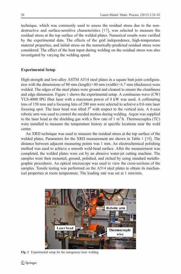
High-strength and low-alloy ASTM A514 steel plates in a square butt-joint configura-tion with the dimensions of 80 mm (length)×40 mm (width)×6.7 mm (thickness) werewelded. The edges of the steel plates were ground and cleaned to ensure the cleanlinessand edge dimension. Figure 1 shows the experimental setup. A continuous wave (CW)YLS-4000 IPG fiber laser with a maximum power of 4 kW was used. A collimatinglens of 150 mm and a focusing lens of 200 mm were selected to achieve a 0.6 mm laserfocusing spot. The laser head was tilted 50 with respect to the vertical axis. A 6-axisrobotic arm was used to control the needed motion during welding. Argon was suppliedto the laser head as the shielding gas with a flow rate of 1 m3/h. Thermocouples (TC)were installed to measure the temperature history at specific locations near the weldcenter.

An XRD technique was used to measure the residual stress at the top surface of thewelded plates. Parameters for the XRD measurement are shown in Table 1 [18]. Thedistance between adjacent measuring points was 1 mm. An electrochemical polishingmethod was used to achieve a smooth weld-bead surface. After the measurement wascompleted, the welded plates were cut by an abrasive water-jet cutting machine. Thesamples were then mounted, ground, polished, and etched by using standard metallo-graphic procedures. An optical microscope was used to view the cross-sections of thesamples. Tensile testing was performed on the A514 steel plates to obtain its mechan-ical properties at room temperature. The loading rate was set at 1 mm/min.

Fig. 1 Experimental setup for the autogenous laser welding

26 Lasers Manuf. Mater. Process. (2015) 2:24–42

Finite Element Model

Governing Equation

The governing equation depicting the spatial and temporal temperature distribution T(x,y, z, t) in the FE model can be specialized to the following differential equation bysolving the Fourier’s second law [19]:

k∇2T−ρCpv∇T þ q•

LASERx; y; z; tð Þ ¼ ρCp

∂T∂t

ð1Þ

where k is thermal conductivity, ρ is material density, Cp is the specific heat of thematerial, v is the velocity of the workpiece, and t is time. The conservation of energy isexpressed in Eq. 1. The convection term in this work was neglected to simplify thenumerical solution. An artificially-increased thermal conductivity was applied when thetemperature was above the melting point in order to compensate for the convective flowof the molten material in the weld pool [20].

Initial condition is specified is:

T x; y; z; 0ð Þ ¼ T0 ð2ÞA lumped heat transfer coefficient is applied to combine heat losses from the model

surfaces based on the Vinokurov’s empirical relationship [21, 22].

h ¼ 2:4� 10−3εT1:61 ð3Þwhere h is the lumped heat transfer coefficient, σ is the Stefan-Boltzmann constant forradiation (5.67×10−8 Wm−2 K−4), and ε is emissivity. The values of ε are presented inTable 2.

Heat Source Model

According to the metallographical images, a cone-shaped fusion zone (FZ) wasachieved by using autogenous laser welding. The heat source model that describes a

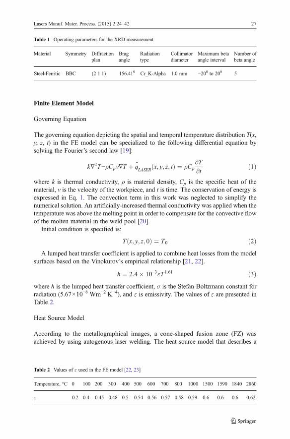
Table 1 Operating parameters for the XRD measurement

Material Symmetry Diffractionplan

Bragangle

Radiationtype

Collimatordiameter

Maximum betaangle interval

Number ofbeta angle

Steel-Ferritic BBC (2 1 1) 156.410 Cr_K-Alpha 1.0 mm −200 to 200 5

Table 2 Values of ε used in the FE model [22, 23]

Temperature, °C 0 100 200 300 400 500 600 700 800 1000 1500 1590 1840 2860

ε 0.2 0.4 0.45 0.48 0.5 0.54 0.56 0.57 0.58 0.59 0.6 0.6 0.6 0.62


conical Gaussian profile is given as the following [24]:

q r; zð Þ ¼ 2P

πr20Yexp 1−

r2

r20

� �1−

y

Y

� �ð4Þ

where P is the laser beam power, r0 is the average keyhole radius, r is the currentradius, y is the current thickness, and Y is the specimen thickness.

Latent Heat of Fusion and Evaporation

In this study, the thermal effect of solid-to-liquid phase transformation was consideredby artificially increasing the specific heat, Cp, in the temperature range between thesolidus and liquidus temperature (TS and TL, respectively). Solid-to-liquid phase trans-formation releases the latent heat of fusion, resulting in an increase in the enthalpy, h,[25].

h ¼ ρCpT þ ρLf f ¼ ρCp0T ð5Þ

where Lf is the latent heat of fusion, ρ is the density, and f is the mass proportion of themolten material, and Cp′ is the artificially-increased specific heat. ρ is set to be constant,and f is given as the following [26]:

f ¼0 T < TS

T−TS

TL−TSTS ≤T ≤TL

1 T > TL

8><>: ð6Þ

When the temperature ranges from TS to TL, the equivalent specific heat Cp' is

extracted from Eq. 6:

Cp0 ¼ Cp þ L

T

T−TS

TL−TSð7Þ

Similarly, when the temperature in the molten pool is above the boiling point (Tb),the latent heat of evaporation (Le) can be considered in the FE model by using theequivalent specific heat Cp″:

Cp″ ¼ C

0p þ

LeT

T−Tb

Tmax−Tbð8Þ

Based on the Eqs. 7 and 8, the specific heat was artificially increased in thetemperature range between the solidus and liquidus temperature and above the boilingpoint. During the thermal analysis, the modified specific heat was added to the“Material Mode” in the software [27].

Mechanical Properties

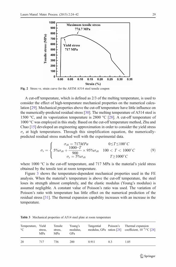
Tensile tests were performed to obtain the mechanical properties of A514 steel at roomtemperature. The results are shown in Fig. 2. Yield stress, Young’s modulus, andTangential modulus of the material at room temperature were achieved, as shown inTable 3.


A cut-off temperature, which is defined as 2/3 of the melting temperature, is used toconsider the effect of high-temperature mechanical properties on the numerical calcu-lation [29]. Mechanical properties above the cut-off temperature have little influence onthe numerically-predicted residual stress [30]. The melting temperature of A514 steel is1500 °C, and its vaporization temperature is 2800 °C [28]. A cut-off temperature of1000 °C was employed in this study. Based on the cut-off temperature method, Zhu andChao [15] developed an engineering approximation in order to consider the yield stressσs at high temperatures. Through this simplification equation, the numerically-predicted residual stress matched well with the experimental data.

σs ¼σs0 ¼ 717MPa 0≤T ≤100�C

5%σs0 þ 1000−T900

� 95%σs0 100 < T < 1000�C

σs ¼ 5%σs0 T ≥1000�C

8><>: ð9Þ

where 1000 °C is the cut-off temperature, and 717 MPa is the material’s yield stressobtained by the tensile test at room temperature.

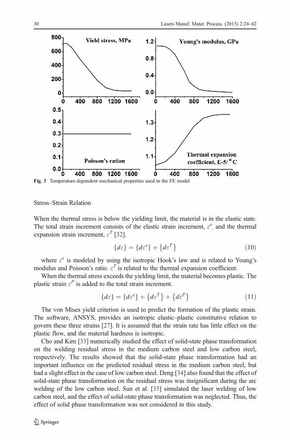
Figure 3 shows the temperature-dependent mechanical properties used in the FEanalysis. When the material’s temperature is above the cut-off temperature, the steelloses its strength almost completely, and the elastic modulus (Young’s modulus) isassumed negligible. A constant value of Poisson’s ratio was used. The variation ofPoisson’s ratio with temperature has little effect on the numerical prediction of theresidual stress [31]. The thermal expansion capability increases with an increase in thetemperature.

Fig. 2 Stress vs. strain curve for the ASTM A514 steel tensile coupon

Table 3 Mechanical properties of A514 steel plate at room temperature

Temperature,°C

Yieldstress,MPa

Tensilestress,MPa

Young’smodulus,GPa

Tangentialmodulus, GPa

Poisson’sration [28]

Thermal expansioncoefficient, 10−5/°C [28]

20 717 736 200 0.911 0.3 1.05


Stress–Strain Relation

When the thermal stress is below the yielding limit, the material is in the elastic state.The total strain increment consists of the elastic strain increment, εe, and the thermalexpansion strain increment, εT [32].

dεf g ¼ dεef g þ dεT� � ð10Þ

where εe is modeled by using the isotropic Hook’s law and is related to Young’smodulus and Poisson’s ratio. εT is related to the thermal expansion coefficient.

When the thermal stress exceeds the yielding limit, the material becomes plastic. Theplastic strain εP is added to the total strain increment.

dεf g ¼ dεef g þ dεT� �þ dεP

� � ð11ÞThe von Mises yield criterion is used to predict the formation of the plastic strain.

The software, ANSYS, provides an isotropic elastic–plastic constitutive relation togovern these three strains [27]. It is assumed that the strain rate has little effect on theplastic flow, and the material hardness is isotropic.

Cho and Kim [33] numerically studied the effect of solid-state phase transformationon the welding residual stress in the medium carbon steel and low carbon steel,respectively. The results showed that the solid-state phase transformation had animportant influence on the predicted residual stress in the medium carbon steel, buthad a slight effect in the case of low carbon steel. Deng [34] also found that the effect ofsolid-state phase transformation on the residual stress was insignificant during the arcwelding of the low carbon steel. Sun et al. [35] simulated the laser welding of lowcarbon steel, and the effect of solid-state phase transformation was neglected. Thus, theeffect of solid phase transformation was not considered in this study.

Fig. 3 Temperature-dependent mechanical properties used in the FE model


Mesh Independence

Figure 4 presents the developed FE model used for the thermal and mechanicalanalysis. Only half of the welded structure was considered due to the symmetry ofthe structure. The mesh was non-linearly graded from fine to coarse size with increas-ing distance away from the weld centerline. The 8-node hexahedral brick element wasapplied to eliminate the negative effect of the degenerated triangle mesh during themechanical analysis. The element type was SOLID70 for the thermal analysis, andSOLID180 for the mechanical analysis. The length of the smallest element in the weldcenter was 0.3 mm (in the longitudinal direction)×0.3 mm (in the transverse direc-tion)×0.4 mm (in the thickness direction). The model contained 92,340 nodes and88,406 elements.

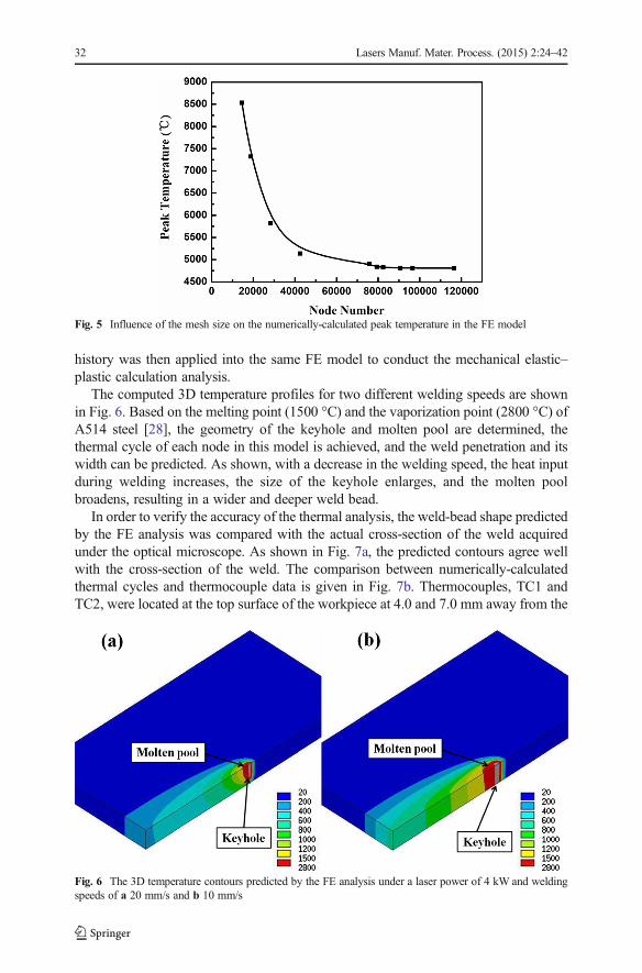
The computing accuracy of the FE analysis relies intensely on the mesh size: thesmaller the mesh size, the more accurate the solution, but the longer the computationaltime [36]. In order to maintain the calculation accuracy and, at the same time, reducethe computing time, the “grid independence” of the FE model, which was related to thecontinuity of the heat flux between adjacent elements, was investigated. A series oftests were conducted in the FE model by using finer meshes under the same materialproperties, element type, and boundary conditions. Only when the solution did notchange with varying mesh size could the results be assumed to be reliable [11]. Fig. 5shows the verification results of the grid independence. As shown, the numericalcalculation of the FE model becomes independent from the mesh size when the numberof nodes in the FE model is above 80,000. The number of nodes in the developed FEmodel should be larger than 80,000 in order to obtain reliable numerical results, butshould be close to 80,000 in order to reduce the computing time.

Results and Discussions

In this work, an uncoupled thermo-mechanical analysis method was conducted tosimulate the autogenous laser welding process [8, 10, 27]. The numerical simulationprocedure consisted of two steps. First, the thermal analysis was conducted to calculatethe temperature history in the welding process. Second, the obtained temperature

(a) (b)

Fig. 4 Geometry and mesh distribution in the developed FE model: a 3D view of the model, b cross-sectionof the model


history was then applied into the same FE model to conduct the mechanical elastic–plastic calculation analysis.

The computed 3D temperature profiles for two different welding speeds are shownin Fig. 6. Based on the melting point (1500 °C) and the vaporization point (2800 °C) ofA514 steel [28], the geometry of the keyhole and molten pool are determined, thethermal cycle of each node in this model is achieved, and the weld penetration and itswidth can be predicted. As shown, with a decrease in the welding speed, the heat inputduring welding increases, the size of the keyhole enlarges, and the molten poolbroadens, resulting in a wider and deeper weld bead.

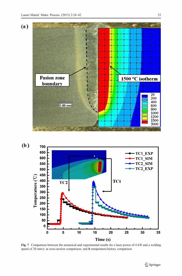
In order to verify the accuracy of the thermal analysis, the weld-bead shape predictedby the FE analysis was compared with the actual cross-section of the weld acquiredunder the optical microscope. As shown in Fig. 7a, the predicted contours agree wellwith the cross-section of the weld. The comparison between numerically-calculatedthermal cycles and thermocouple data is given in Fig. 7b. Thermocouples, TC1 andTC2, were located at the top surface of the workpiece at 4.0 and 7.0 mm away from the

Fig. 5 Influence of the mesh size on the numerically-calculated peak temperature in the FE model

Fig. 6 The 3D temperature contours predicted by the FE analysis under a laser power of 4 kW and weldingspeeds of a 20 mm/s and b 10 mm/s


(a )

(b )

)

)

Fig. 7 Comparison between the numerical and experimental results for a laser power of 4 kW and a weldingspeed of 20 mm/s: a cross-section comparison; and b temperature-history comparison


weld centerline, respectively. As shown in Fig. 7b, the thermal cycles obtained by theFE analysis match well with the experimental results. Good agreement between theexperimental and numerical results verifies the accuracy of the selected heat sourcemodel and thermal boundary conditions.

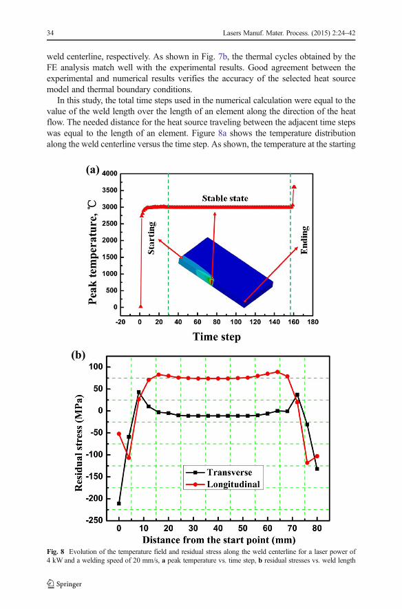
In this study, the total time steps used in the numerical calculation were equal to thevalue of the weld length over the length of an element along the direction of the heatflow. The needed distance for the heat source traveling between the adjacent time stepswas equal to the length of an element. Figure 8a shows the temperature distributionalong the weld centerline versus the time step. As shown, the temperature at the starting

(a)

(b)

Fig. 8 Evolution of the temperature field and residual stress along the weld centerline for a laser power of4 kW and a welding speed of 20 mm/s, a peak temperature vs. time step, b residual stresses vs. weld length


stage is rising from 20 to 3000 °C with the time steps ranging from 2 to 30. Thetemperature increases sharply, and the temperature gradient between adjacenttime steps is large. With the moving of the heat source along the weldingdirection, the temperature difference gradually decreases to zero, and thewelding process reaches a steady state. The heat flux is uniformly distributedin the FE model at the steady-state stage, indicating that there is no variation inthe heat flux between adjacent elements. Correspondingly, the distributions ofthe transverse and longitudinal residual stresses are uniform along the weldcenterline at the steady-state stage (see Fig. 8b). When the heat source ap-proaches the final part of this model, the temperature rises again due to theedge effect. At the edge of this FE model, the heat lost induced by theconvection and radiation decreases with an increase in the surface area incontact with the air. The heat transfer coefficient of the material is larger thanthat of the air, leading to the rise of temperature profiles. At the starting andending stages, there exist large temperature gradients between adjacent ele-ments, leading to the large variation in the values of residual stresses. Theuniform distributions of residual stresses are achieved when the temperaturegradient between adjacent elements is zero.

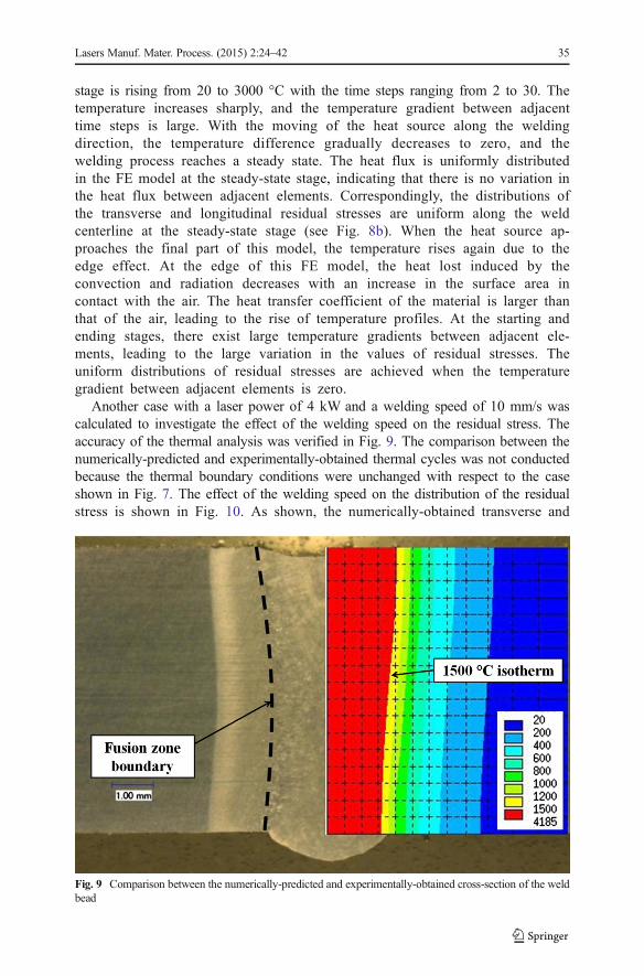
Another case with a laser power of 4 kW and a welding speed of 10 mm/s wascalculated to investigate the effect of the welding speed on the residual stress. Theaccuracy of the thermal analysis was verified in Fig. 9. The comparison between thenumerically-predicted and experimentally-obtained thermal cycles was not conductedbecause the thermal boundary conditions were unchanged with respect to the caseshown in Fig. 7. The effect of the welding speed on the distribution of the residualstress is shown in Fig. 10. As shown, the numerically-obtained transverse and

Fig. 9 Comparison between the numerically-predicted and experimentally-obtained cross-section of the weldbead


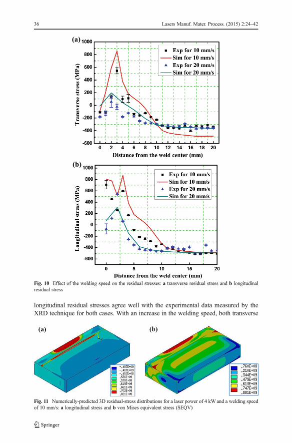
longitudinal residual stresses agree well with the experimental data measured by theXRD technique for both cases. With an increase in the welding speed, both transverse

(a)

(b)

Fig. 10 Effect of the welding speed on the residual stresses: a transverse residual stress and b longitudinalresidual stress

Fig. 11 Numerically-predicted 3D residual-stress distributions for a laser power of 4 kWand a welding speedof 10 mm/s: a longitudinal stress and b von Mises equivalent stress (SEQV)


and longitudinal residual stresses experience a general decrease due to a decrease in theheat input during welding.

The FE analysis results give detailed information about 3D residual-stress fieldinside the welded structure. Figure 11 shows the predicted distribution of the longitu-dinal stress and the von Mises equivalent stress (SEQV). As shown, SEQV in the weldzone has a magnitude larger than 747 MPa. The yielding stress of the A514 steel is717 MPa. Thus, there are the plastic strains and residual stress retained in the weld zoneand its vicinity. As shown in Fig. 11 a and b, the high tensile residual stress isconcentrated in the middle section of the developed model. This may be caused bythe small size of the FE model.

The FE mechanical analysis gives detailed spatial and temporal information about theevolution and distribution of the residual stress. Figure 12 shows the variation of theresidual stress as a function of the welding time along the line AB. As shown in Fig. 12d,the line AB is located in the middle of the weld. The time when the laser head reaches theline AB is 4.0 s. When the laser beam (heat source) is away from the line AB (t≤3.5 s), ahigh compressive stress (initial stress) is presented in the weld zone and base material.When the laser beam approaches the line AB, the temperature of the material near the lineAB increases, resulting in the expansion of the heated material. The expansion is inhibitedby the surrounding material, resulting in an increase in the longitudinal compressive stress(3.5 s<t<4.0 s). With respect to the longitudinal stress, the transverse stress has little

(a) (b)

Fig. 12 Residual stresses vs. welding time for a laser power of 4 kW and a welding speed of 10 mm/s, atransverse stress, b longitudinal stress, c von Mises equivalent stress, and d temperature contours at a time of3.9 s


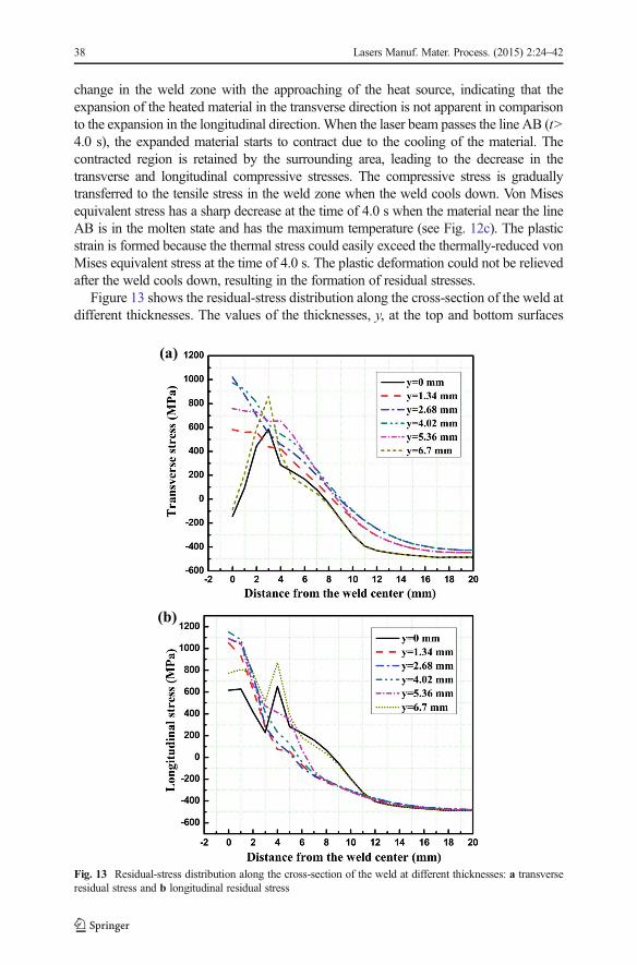
change in the weld zone with the approaching of the heat source, indicating that theexpansion of the heated material in the transverse direction is not apparent in comparisonto the expansion in the longitudinal direction. When the laser beam passes the line AB (t>4.0 s), the expanded material starts to contract due to the cooling of the material. Thecontracted region is retained by the surrounding area, leading to the decrease in thetransverse and longitudinal compressive stresses. The compressive stress is graduallytransferred to the tensile stress in the weld zone when the weld cools down. Von Misesequivalent stress has a sharp decrease at the time of 4.0 s when the material near the lineAB is in the molten state and has the maximum temperature (see Fig. 12c). The plasticstrain is formed because the thermal stress could easily exceed the thermally-reduced vonMises equivalent stress at the time of 4.0 s. The plastic deformation could not be relievedafter the weld cools down, resulting in the formation of residual stresses.

Figure 13 shows the residual-stress distribution along the cross-section of the weld atdifferent thicknesses. The values of the thicknesses, y, at the top and bottom surfaces

(a)

(b)

Fig. 13 Residual-stress distribution along the cross-section of the weld at different thicknesses: a transverseresidual stress and b longitudinal residual stress


are 6.7 and 0 mm, respectively. It is noted that in the weld zone, the distributions ofresidual stresses at the top and bottom surface are similar but are different from thestress distribution inside the weld bead. For the transverse residual stress (see Fig. 13a),a compressive stress is presented at the top and bottom surfaces in the weld center.However, a high tensile transverse stress exists inside the weld bead. In the case oflongitudinal residual stress (see Fig. 13b), the tensile longitudinal stress is located in theweld zone for all positions along the weld thickness direction. However, the longitu-dinal stress presented inside the weld bead has a higher value than the stress located atthe top and bottom surfaces.

Before welding, the residual stress at the top surface of A514 steel was measured bythe XRD technique. The results are shown in Fig. 14. When measuring the initialstresses, the square map was chosen to settle the measurement points [18]. The pointswere measured along the edges of the square and then interpolated. As shown, atransverse compressive stress of around 350 MPa and a longitudinal compressive stressof around 500 MPa are presented at the top surface of the A514 steel plate. These highcompressive residual stresses were introduced by the preceding manufacturing pro-cesses and presented in the steel plate as initial stress. The effect of initial stress on thenumerical simulation was investigated. “INISTATE” command in the ANSYS softwarewas used to apply initial stress on the element-based FE model. This command was

0 5 10 15 20 25 30 35 40

0

2

4

6

8

10-400

-300

-200

X-axis (mm)

Y-axis (mm)

Tra

nsve

rse

stre

ss (M

Pa)

0

10

20

30

40

02

46

810

-600

-400

-200

X-axis (mm)Y-axis (mm)

Long

itudi

nal s

tres

s (M

Pa)

(a)

(b)

Fig. 14 Initial stresses presented in the base material: a transverse stress and b longitudinal stress


coded by using the ANSYS Program Design Language. It was assumed that allelements in the FE model had the same distribution of initial stress. Transverse andlongitudinal initial stresses defined as −350 and −500 MPa, respectively, were added toall elements in the FE model.

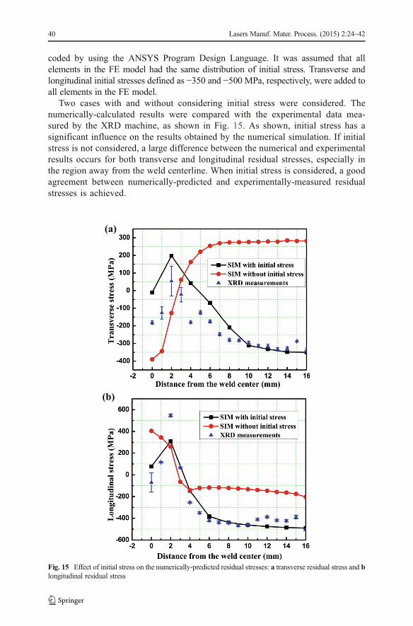
Two cases with and without considering initial stress were considered. Thenumerically-calculated results were compared with the experimental data mea-sured by the XRD machine, as shown in Fig. 15. As shown, initial stress has asignificant influence on the results obtained by the numerical simulation. If initialstress is not considered, a large difference between the numerical and experimentalresults occurs for both transverse and longitudinal residual stresses, especially inthe region away from the weld centerline. When initial stress is considered, a goodagreement between numerically-predicted and experimentally-measured residualstresses is achieved.

(a)

(b)

Fig. 15 Effect of initial stress on the numerically-predicted residual stresses: a transverse residual stress and blongitudinal residual stress


Conclusions

A 3D FE model was developed to simulate the thermal field and thermally-inducedresidual stress during autogenous laser welding of high-strength steel. Importantconclusions are presented as the following:

1) Tensile testing was conducted on the base material in order to achieve themechanical properties at room temperature. The mechanical properties at hightemperatures were then simplified through a cut-off temperature method.

2) The grid independence of the FE model was verified to guarantee the continuity ofthe heat flux between adjacent elements. Uniform distribution of temperaturedetermined the consistency of residual stress predicted in the FE model.

3) The thermal and mechanical results obtained by the FE analysis agreed well withthe experimental results measured by an XRD technique. The verified numericalresults provided detailed information about the evolution and distribution ofresidual stress during welding.

4) Two cases with different welding speed were modeled in this work. It was foundthat with an increase in the welding speed, both transverse and longitudinalresidual stresses decreased due to a decrease in the heat input during welding.

5) A514 steel plates used for welding had a high compressive initial stress. Asubroutine was developed to consider the effect of initial stress on the FE analysis.It was found that a big discrepancy between experimental and numerical resultsoccurred when initial stress was not considered in the FE model.

Acknowledgments The financial support by NSF’s Grant No. IIP-1034652 is acknowledged. The authorsalso would like to thank the engineer Andrew Socha for the help in the execution of experiments.

References

1. Ma, J., Kong, F., Liu, W., Carlson, B., Kovacevic, R.: Study on the strength and failure modes of laserwelded galvanized DP980 steel lap joints. J. Mater. Process. Technol. 214(8), 1696–1709 (2014)

2. Liu, W., Liu, S., Ma, J., Kovacevic, R.: Real-time monitoring of the laser hot-wire welding process. Opt.Laser Technol. 57, 66–76 (2014)

3. Liu, W., Ma, J., Yang, G., Kovacevic, R.: Hybrid laser-arc welding of advanced high-strength steel. J.Mater. Process. Technol. 214(12), 2823–2833 (2014)

4. Colegrove, P., Ikeagu, C., Thistlethwaite, A., Williams, S., Nagy, T., Suder, W., Steuwer, A., Pirling, T.:Welding process impact on residual stresses and distortion. Sci. Technol. Weld. Join. 14, 717–725 (2009)

5. Hatamleh, O., Rivero, I., Lyons, J.: Evaluation of surface residual stresses in friction stir welds due to laserand shot peening. J. Mater. Eng. Perform. 16, 549–553 (2007)

6. Qian, Z., Chumbley, S., Karakulak, T., Johnson, E.: The residual stress relaxation behavior of weldmentsduring cyclic loading. Metall. Mater. Trans. A 44(7), 3147–3156 (2013)

7. Gong X, Anderson T, Chou K.: Review on powder-based electron beam additive manufacturing technol-ogy. In ASME/ISCIE 2012 International Symposium on Flexible Automation. American Society ofMechanical Engineers, (pp. 507–515) (2012)

8. Deng, D., Luo, Y., Serizawa, H., Shibahara, M., Murakawa, H.: Numerical simulation of residual stressesand deformation considering phase transformation effect. Trans. JWRI 32, 325–333 (2003)

9. Zain-ul-Abdein, M., Nelias, D., Jullien, J., Deloison, D.: Prediction of laser beam welding-induceddistortions and residual stresses by numerical simulation for aeronautic application. J. Mater. Process.Technol. 209, 2907–2917 (2009)


10. Kong, F., Ma, J., Kovacevic, R.: Numerical and experimental study of thermally induced residual stress inthe hybrid laser–GMAwelding process. J. Mater. Process. Technol. 211(6), 1102–1111 (2011)

11. Gross, M.: Comprehensive numerical simulation of laser materials processing. In: Dowden, J. (ed.) Thetheory of laser materials processing: heat and mass transfer in modern technology, pp. 339–380. Springer,New York (2009)

12. Radaj, D.: Welding residual stresses and distortion: calculation and measurement, 2nd edn, pp. 118–200.Verlag für Schweissen und Verwandte Verfahren, DVS-Verlag (2003)

13. Heinze, C., Schwenk, C., Rethmeier, M.: Influences of mesh density and transformation behavior on theresult quality of numerical calculation of welding induced distortion. Simul. Model. Pract. Theory 19,1847–1859 (2011)

14. Blodgett, O.: Types and causes of distortion in welded steel and corrective measures. Weld. J. 39, 692–697(1960)

15. Zhu, X., Chao, Y.: Effects of temperature-dependent material properties on welding simulation. Comput.Struct. 80, 967–976 (2002)

16. Tsai, C., Kim, D.: Understanding residual stresses and distortion in welds: an overview. Processes andmechanisms of welding residual stresses and distortion. In: Feng, Z. (ed.) Processes and mechanisms ofwelding residual stresses and distortion, pp. 3–6. CRC Press, Florida (2005)

17. Qian, Z., Chumbley, S., Johnson, E.: The effect of specimen dimension on residual stress relaxation ofcarburized and quenched steels. Mater. Sci. Eng. A 529, 246–252 (2011)

18. Liu W, Kong F, Kovacevic R.: Residual Stress Analysis and Weld Bead Shape Study in Laser Welding ofHigh Strength Steel. In ASME 2013 International Manufacturing Science and Engineering Conferencecollocated with the 41st North American Manufacturing Research Conference. American Society ofMechanical Engineers, pp. V001T01A053-V001T01A053, (2013)

19. Steen, W., Mazumder, J.: Laser material processing, 4th edn, pp. 255–257. Springer, New York (2010)20. Farahmand, P., Kovacevic, R.: An experimental–numerical investigation of heat distribution and stress

field in single-and multi-track laser cladding by a high-power direct diode laser. Opt. Laser Technol. 63,154–168 (2014)

21. Bag, S., Trivedi, S., De, A.: Development of a finite element based heat transfer model for conductionmode laser spot welding process using an adaptive volumetric heat source. Int. J. Therm. Sci. 48, 1923–1931 (2009)

22. Frewin, M.R., Scott, D.A.: Finite element modal of pulsed laser welding.Weld. Res. Suppl. 78, 15–22 (1999)23. Brown, S., Song, H.: Finite element simulation of welding of large structures. J. Manuf. Sci. Eng. 114,

441–451 (1992)24. Tsirkas, S., Papanikos, P., Kermanidis, T.: Numerical simulation of the laser welding process in butt-joint

specimens. J. Mater. Process. Technol. 134, 59–69 (2003)25. Cho, J., Na, S.: Three-dimensional analysis of molten pool in GMA-laser hybrid welding. Weld. J. 88, 35–

43 (2009)26. Piekarska, W., Kubiak, M.: Three-dimensional model for numerical analysis of thermal phenomena in

laser–arc hybrid welding process. Int. J. Heat Mass Transf. 54, 4966–4974 (2011)27. ANSYS Inc.: ANSYS 11.0 manual (2007)28. Kong, F., Kovacevic, R.: Development of a comprehensive process model for hybrid laser-Arc welding.

In: Kovacevic, R. (ed.) Welding processes, pp. 164–174. Intech, New York (2012)29. Tekrewal, P.: Transient and residual thermal strain–stress analysis of GMAW. Trans. ASME J. Eng. Mater.

Technol 113, 336–343 (1991)30. Börjesson, L., Lindgren, L.: Simulation of multipass welding with simultaneous computation of material

properties. J. Eng. Mater. Technol. 123, 106–111 (2001)31. Tekriwal, P., Mazumder, J.: Transient and residual thermal strain–stress analysis of GMAW. J. Eng. Mater.

Technol. 113(3), 336–343 (1991)32. Li, C., Wang, Y., Zhan, H., Han, T., Han, B., Zhao, W.: Three-dimensional finite element analysis of

temperatures and stresses in wide-band laser surfacemelting processing.Mater. Des. 31(7), 3366–3373 (2010)33. Cho, S.H., Kim, J.W.: Analysis of residual stress in carbon steel weldment incorporating phase transfor-

mations. Sci. Technol. Weld. Join. 7(4), 212–216 (2002)34. Deng, D.: FEM prediction of welding residual stress and distortion in carbon steel considering phase

transformation effects. Mater. Des. 30(2), 359–366 (2009)35. Sun, J., Liu, X., Tong, Y., Deng, D.: A comparative study on welding temperature fields, residual stress

distributions and deformations induced by laser beam welding and CO2 gas arc welding. Mater. Des. 63,519–530 (2014)

36. Komanduri, R., Hou, Z.: Thermal analysis of the arc welding process: Part I. General solutions. Metall.Mater. Trans. B 31, 1353–1370 (2000)


numerical modeling and experimental verification of

Documents